Guide for Selecting Manning's Roughness Coefficients for

Guide for Selecting Manning's Roughness Coefficients for Natural Channels and Flood Plains

United States Geological SurveyWater-Supply Paper 2339

Prepared in cooperation with the United States Department of Transportation, Federal Highway Administration


By GEORGE J. ARCEMENT, JR., and VERNE R. SCHNEIDER

Prepared in cooperation with the U.S. Department of Transportation, Federal Highway Administration

A guide presenting step-by-step procedures for selecting Manning's roughness coefficient, n, for natural channels and flood plains. Photographs of flood-plain segments can be used for comparison with similar flood plains to aid in assigning n values

U.S. GEOLOGICAL SURVEY WATER-SUPPLY PAPER 2339

DEPARTMENT OF THE INTERIOR

MANUEL LUJAN, Jr., Secretary

U.S. GEOLOGICAL SURVEY

Dallas L. Peck, Director

Any use of trade, product, or firm names in this publication is for descriptive purposes only and does not imply endorsement by the U.S. Government

UNITED STATES GOVERNMENT PRINTING OFFICE: 1989

For sale by theBooks and Open-File Reports Section,U.S. Geological Survey,Federal Center, Box 25425,Denver, CO 80225

Library of Congress Cataloging in Publication Data

Arcement, George J.Guide for selecting Manning's roughness coefficients for natural channels

and flood plains.

(Water-supply paper / United States Geological Survey ; 2339)"Prepared in cooperation with U.S. Department of Transportation, Federal

Highway Administration."Bibliography: p.Supt. of Docs. no. : I 19.13:23391. Channels (Hydraulic engineering). 2. Flood plains. 3. Frictional resis

tance (Hydrodynamics). I. Schneider, V. R. II. United States. Federal Highway Administration. III. Title. IV. Title: Manning's roughness coefficients for natural channels and flood plains. V. Series: U.S. Geo logical Survey water-supply paper ; 2339.

TC175.A67 1989 627'.4 88-600129

CONTENTS

Abstract 1 Introduction 1 Methods 2 Channel n Values 2

Base n Values (nb) for Channels 2 Adjustment Factors for Channel n Values 6

Irregularity (HJ) 6Variation in Channel Cross Section («2) 6 Obstructions (n3) 6 Vegetation («4) 6 Meandering (m) 8

Rood-Plain n Values 8Modified Channel Method 8

Adjustment Factors for Flood-Plain n Values 8 Surface Irregularities (HJ) 8 Obstructions («3) 8 Vegetation (n4) 8

Vegetation-Density Method 9Techniques for Determining Vegetation Density 9

Indirect Technique 10 Direct Technique 10

Photographs of Flood Plains 13 Procedures for Assigning n Values 28

Steps for Assigning n Values 28Reach Subdivision (Steps 1 and 2) 28 Channel Roughness (Steps 3-13) 28 Rood-Plain Roughness (Steps 14-23) 29

Examples of Procedures for Determining n Values 32 Summary 32 References Cited 37

FIGURES

1. Diagram of a schematic and cross sections of a hypothetical reach of achannel and flood plain showing subdivisions used in assigning n values 3

2. Graph showing relation of stream power and median grain size to flow regime 5

3. Diagram showing forms of bed roughness in sand-bed channels 54. Graph showing effective-drag coefficient for verified n values versus the

hydraulic radius of wide, wooded flood plains 105. Chart of example measurement of vegetation density showing tree diameter

and location in representative sample area 12

Contents III

6-20. Photographs showing flood plains having verified n values:6. Cypress Creek near Downsville, La., Vegrf=0.0067 137. Bayou de Loutre near Farmerville, La., Vegd=0.0061 148. Bayou de Loutre near Farmerville, La., Vegd=0.0015 159. Bayou de Loutre near Farmerville, La., Vegd=0.0012 16

10. Coldwater River near Red Banks, Miss., Vegd=0.0011 1711. Coldwater River near Red Banks, Miss., Vegd=0.0090 1812. Yockanookany River near Thomastown, Miss., Vegd=0. 0082 1913. Yockanookany River near Thomastown, Miss., 500 ft east of

area shown in figure 12, Vegd =O.QQS2 2014. Flagon Bayou near Libuse, La., Vegd =O.QQSl 2115. Pea Creek near Louisville, Ala., Vegd=O.OOS5 2216. Pea Creek near Louisville, Ala., V<?grf=0.0102 2317. Tenmile Creek near Elizabeth, La., V<?^=0.0067 2418. Sixmile Creek near Sugartown, La., Vegd=O.OOS4 2519. Thompson Creek near Clara, Miss., Vegd=0.0l\5 26 20. Thompson Creek near Clara, Miss., 500 ft east of area shown

in figure 19, Vegd =O.OU5 2721. Flow chart of procedures for assigning n values 3022. Sample form for computing n values 33

TABLES

1. Base values of Manning's n 42. Adjustment values for factors that affect the roughness of a channel 73. Adjustment values for factors that affect the roughness of flood plains 94. Outline and example of procedures for determining n values for a hypothetical

channel and adjoining flood plain 35

METRIC CONVERSION FACTORS

For readers who wish to convert measurements from the inch-pound system of units to the metric system

of units, the conversion factors are listed below:

Multiply inch-pound unit By To obtain metric unit

cubic foot per second (ft3/s) 0.02832 cubic meter per second (m3/s)foot (ft) .3048 meter (m)

foot per second (ft/s) .3048 meter per second (m/s)foot per square second (ft/s2) .3048 meter per square second (m/s2)

inch (in.) 25.40 millimeter (mm)square foot (ft2 ) .0929 square meter (m2)

pounds per square foot (lb/ft2) 4.882 kilograms per square meter (km/m2)

IV Contents

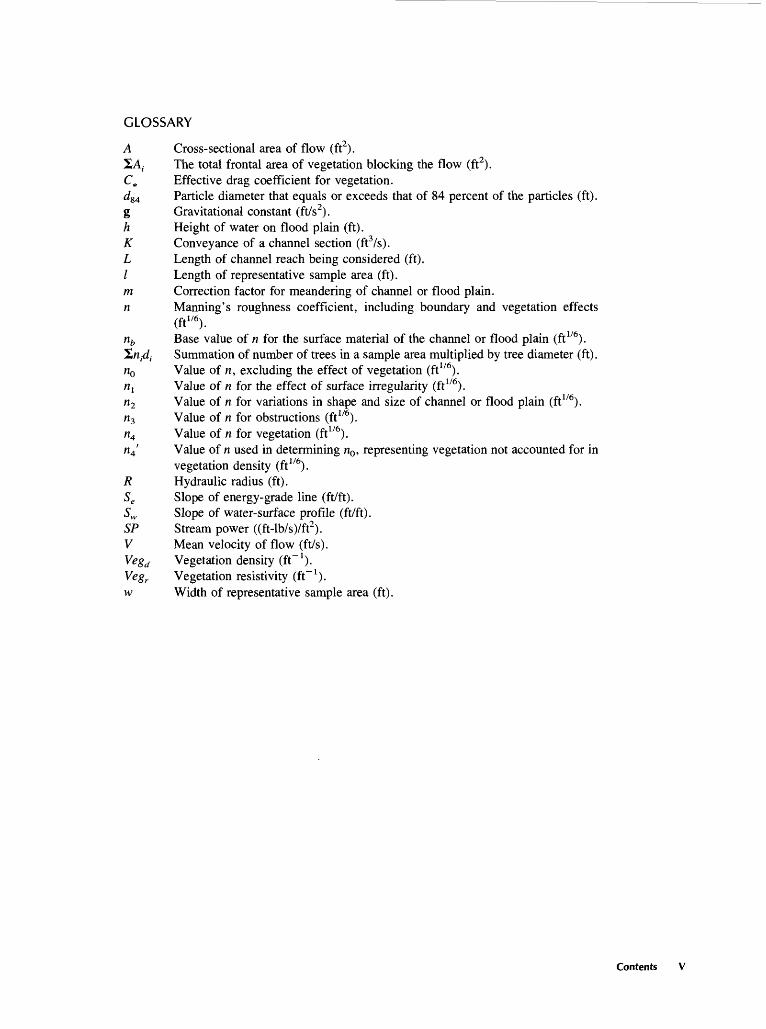
GLOSSARY

A Cross-sectional area of flow (ft2).SA,. The total frontal area of vegetation blocking the flow (ft2).C* Effective drag coefficient for vegetation.dS4 Particle diameter that equals or exceeds that of 84 percent of the particles (ft).g Gravitational constant (ft/s2).h Height of water on flood plain (ft).K Conveyance of a channel section (ft3/s).L Length of channel reach being considered (ft)./ Length of representative sample area (ft).m Correction factor for meandering of channel or flood plain.n Manning's roughness coefficient, including boundary and vegetation effects

(ft176).

% Base value of n for the surface material of the channel or flood plain (ft1/6)."Zrijdj Summation of number of trees in a sample area multiplied by tree diameter (ft).^ Value of n, excluding the effect of vegetation (ft 176).nl Value of n for the effect of surface irregularity (ft1/6).n2 Value of n for variations in shape and size of channel or flood plain (ft 176).% Value of n for obstructions (ft 176).n4 Value of n for vegetation (ft1/6).n4 ' Value of n used in determining n0 , representing vegetation not accounted for in

vegetation density (ft 176). R Hydraulic radius (ft). Se Slope of energy-grade line (ft/ft). Sw Slope of water-surface profile (ft/ft). SP Stream power ((ft-lb/s)/ft2). V Mean velocity of flow (ft/s). Ve8d Vegetation density (ft" 1 ). Vegr Vegetation resistivity (ft~ l ). w Width of representative sample area (ft).

Contents


By George J. Arcement, Jr., and Verne R. Schneider

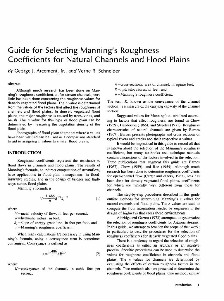
Abstract

Although much research has been done on Man ning's roughness coefficient, n, for stream channels, very little has been done concerning the roughness values for densely vegetated flood plains. The n value is determined from the values of the factors that affect the roughness of channels and flood plains. In densely vegetated flood plains, the major roughness is caused by trees, vines, and brush. The /? value for this type of flood plain can be determined by measuring the vegetation density of the flood plain.

Photographs of flood-plain segments where n values have been verified can be used as a comparison standard to aid in assigning n values to similar flood plains.

INTRODUCTION

Roughness coefficients represent the resistance to flood flows in channels and flood plains. The results of Manning's formula, an indirect computation of streamflow, have applications in flood-plain management, in flood- insurance studies, and in the design of bridges and high ways across flood plains.

Manning's formula is

^1486^2/3,1/2 (1)

whereV=mean velocity of flow, in feet per second, R= hydraulic radius, in feet, Se = slope of energy grade line, in feet per foot, and n=Manning's roughness coefficient.

When many calculations are necessary in using Man ning's formula, using a conveyance term is sometimes convenient. Conveyance is defined as

K=-1.486-AR2/3 (2)

whereK=conveyance of the channel, in cubic feet per

second,

A = cross-sectional area of channel, in square feet, R = hydraulic radius, in feet, and n= Manning's roughness coefficient.

The term K, known as the conveyance of the channel section, is a measure of the carrying capacity of the channel section.

Suggested values for Manning's n, tabulated accord ing to factors that affect roughness, are found in Chow (1959), Henderson (1966), and Streeter (1971). Roughness characteristics of natural channels are given by Barnes (1967). Barnes presents photographs and cross sections of typical rivers and creeks and their respective n values.

It would be impractical in this guide to record all that is known about the selection of the Manning's roughness coefficient, but many textbooks and technique manuals contain discussions of the factors involved in the selection. Three publications that augment this guide are Barnes (1967), Chow (1959), and Ree (1954). Although much research has been done to determine roughness coefficients for open-channel flow (Carter and others, 1963), less has been done for densely vegetated flood plains, coefficients for which are typically very different from those for channels.

The step-by-step procedures described in this guide outline methods for determining Manning's n values for natural channels and flood plains. The n values are used to compute the flow information needed by engineers in the design of highways that cross these environments.

Aldridge and Garrett (1973) attempted to systematize the selection of roughness coefficients for Arizona streams. In this guide, we attempt to broaden the scope of that work; in particular, to describe procedures for the selection of roughness coefficients for densely vegetated flood plains.

There is a tendency to regard the selection of rough ness coefficients as either an arbitrary or an intuitive process. Specific procedures can be used to determine the values for roughness coefficients in channels and flood plains. The n values for channels are determined by evaluating the effects of certain roughness factors in the channels. Two methods also are presented to determine the roughness coefficients of flood plains. One method, similar

Introduction

to that for channel roughness, involves the evaluation of the effects of certain roughness factors in the flood plain. The other method involves the evaluation of the vegetation density of the flood plain to determine the n value. This second method is particularly suited to handle roughness for densely wooded flood plains. Photographs of flood plains that have known n values are presented for comparison to flood plains that have unknown n values.

METHODS

Values of the roughness coefficient, n, may be assigned for conditions that exist at the time of a specific flow event, for average conditions over a range in stage, or for anticipated conditions at the time of a future event. The procedures described in this report are limited to the selection of roughness coefficients for application to one- dimensional, open-channel flow. The values are intended mostly for use in the energy equation as applied to one- dimensional, open-channel flow, such as in a slope-area or step-backwater procedure for determining flow.

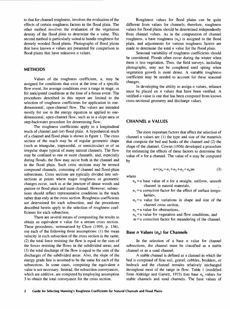
The roughness coefficients apply to a longitudinal reach of channel and (or) flood plain. A hypothetical reach of a channel and flood plain is shown in figure 1. The cross section of the reach may be of regular geometric shape (such as triangular, trapezoidal, or semicircular) or of an irregular shape typical of many natural channels. The flow may be confined to one or more channels, and, especially during floods, the flow may occur both in the channel and in the flood plain. Such cross sections may be termed compound channels, consisting of channel and flood-plain subsections. Cross sections are typically divided into sub sections at points where major roughness or geometric changes occur, such as at the juncture of dense woods and pasture or flood plain and main channel. However, subsec tions should reflect representative conditions in the reach rather than only at the cross section. Roughness coefficients are determined for each subsection, and the procedures described herein apply to the selection of roughness coef ficients for each subsection.

There are several means of compositing the results to obtain an equivalent n value for a stream cross section. These procedures, summarized by Chow (1959, p. 136), use each of the following three assumptions: (1) the mean velocity in each subsection of the cross section is the same;(2) the total force resisting the flow is equal to the sum of the forces resisting the flows in the subdivided areas; and(3) the total discharge of the flow is equal to the sum of the discharges of the subdivided areas. Also, the slope of the energy grade line is assumed to be the same for each of the subsections. In some cases, computing the equivalent n value is not necessary. Instead, the subsection conveyances, which are additive, are computed by employing assumption 3 to obtain the total conveyance for the cross section.

Roughness values for flood plains can be quite different from values for channels; therefore, roughness values for flood plains should be determined independently from channel values. As in the computation of channel roughness, a base roughness (nb) is assigned to the flood plain, and adjustments for various roughness factors are made to determine the total n value for the flood plain.

Seasonal variability of roughness coefficients should be considered. Floods often occur during the winter when there is less vegetation. Thus, the field surveys, including photographs, may not be completed until spring when vegetation growth is more dense. A variable roughness coefficient may be needed to account for these seasonal changes.

In developing the ability to assign n values, reliance must be placed on n values that have been verified. A verified n value is one that has been computed from known cross-sectional geometry and discharge values.

CHANNEL n VALUES

The most important factors that affect the selection of channel n values are (1) the type and size of the materials that compose the bed and banks of the channel and (2) the shape of the channel. Cowan (1956) developed a procedure for estimating the effects of these factors to determine the value of n for a channel. The value of n may be computed by

n=(nb +n 1 +n2 +n3 +n4)m (3)

wherenb =a. base value of n for a straight, uniform, smooth

channel in natural materials, ,/ij =a correction factor for the effect of surface irregu

larities,«2 =a value for variations in shape and size of the

channel cross section,«3 =a value for obstructions,n4 =a value for vegetation and flow conditions, andm =a correction factor for meandering of the channel.

Base n Values (nh) for Channels

In the selection of a base n value for channel subsections, the channel must be classified as a stable channel or as a sand channel.

A stable channel is defined as a channel in which the bed is composed of firm soil, gravel, cobbles, boulders, or bedrock and the channel remains relatively unchanged throughout most of the range in flow. Table 1 (modified from Aldridge and Garrett, 1973) lists base nb values for stable channels and sand channels. The base values of

2 Guide for Selecting Manning's Roughness Coefficients for Natural Channels and Flood Plains

oooooo oooooo

ooooo ooooo

o Cotton o fields oooooooooo

ft 10-8-

6-

4-

Water surface

20 40 60ft

CROSS SECTION 1

Segments 1 2 3

80ft

CROSS SECTION 2

Subsections 2

I I 1,000'

I I I 30' I

I 1,000' I

CROSSSECTION

3

(Not to scale)

CROSS SECTION 3

Figure 1. A schematic and cross sections of a hypothetical reach of a channel and flood plain showing subdivisions used in assigning n values.

Benson and Dalrymple (1967) apply to conditions that are close to average, whereas Chow's (1959) base values are for the smoothest reach attainable for a given bed material.

Barnes (1967) cataloged verified n values for stable channels having roughness coefficients ranging from 0.024 to 0.075. In addition to a description of the cross section,

bed material, and flow conditions during the measurement, color photographs of the channels were provided.

A sand channel is defined as a channel in which the bed has an unlimited supply of sand. By definition, sand ranges in grain size from 0.062 to 2 mm. Resistance to flow varies greatly in sand channels because the bed material

Channel n Values

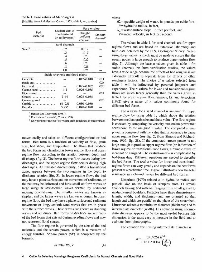
Table 1. Base values of Manning's n[Modified from Aldridge and Garrett, 1973, table 1; , no data]

Bed material

Median size of bed material

(in millimeters)

Base n value

Straight uniform channel1

Smooth channel2

Sand channels

Sand3 .......... ........ 0.2.3 .4 .5 .6 .8

1.0

0.012 .017 .020 .022 .023 .025 .026

Stable channels and flood plains

Concrete .......Rock cut .......

Coarse sand ....Fine gravel .....

Coarse gravel . . .Cobble.........Boulder ........

_

........ 1-2

........ 2-64

........ 64-256

........ >256

0.012-0.018

0.025-0.032 0.026-0.035

0.028-0.035

0.030-0.050 0.040-0.070

0.011 .025 .020

.024

.026

1 Benson and Dalrymple (1967).2 For indicated material; Chow (1959).3 Only for upper regime flow where grain roughness is predominant.

moves easily and takes on different configurations or bed forms. Bed form is a function of velocity of flow, grain size, bed shear, and temperature. The flows that produce the bed forms are classified as lower regime flow and upper regime flow, according to the relation between depth and discharge (fig. 2). The lower regime flow occurs during low discharges, and the upper regime flow occurs during high discharges. An unstable discontinuity, called a transitional zone, appears between the two regimes in the depth to discharge relation (fig. 3). In lower regime flow, the bed may have a plane surface and no movement of sediment, or the bed may be deformed and have small uniform waves or large irregular saw-toothed waves formed by sediment moving downstream. The smaller waves are known as ripples, and the larger waves are known as dunes. In upper regime flow, the bed may have a plane surface and sediment movement or long, smooth sand waves that are in phase with the surface waves. These waves are known as standing waves and antidunes. Bed forms on dry beds are remnants of the bed forms that existed during receding flows and may not represent flood stages.

The flow regime is governed by the size of the bed materials and the stream power, which is a measure of energy transfer. Stream power (SP) is computed by the formula:

where62= specific weight of water, in pounds per cubic foot,/?=hydraulic radius, in feet,

Sw = water-surface slope, in feet per foot, andV=mean velocity, in feet per second.

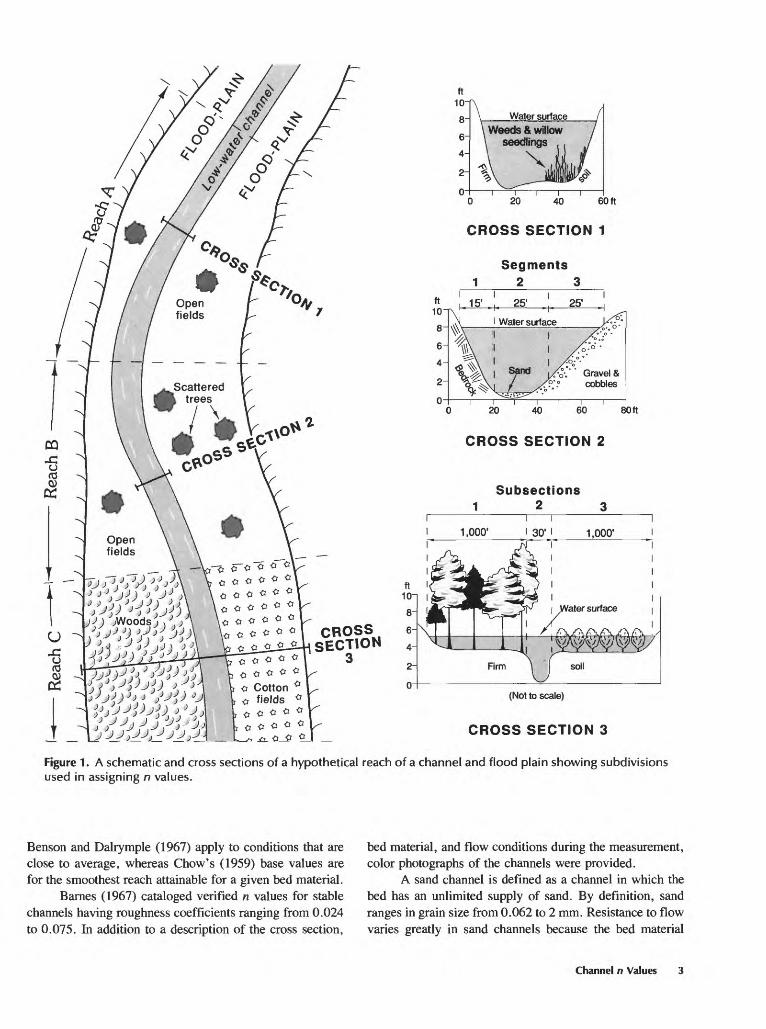
The values in table 1 for sand channels are for upper regime flows and are based on extensive laboratory and field data obtained by the U.S. Geological Survey. When using these values, a check must be made to ensure that the stream power is large enough to produce upper regime flow (fig. 2). Although the base n values given in table 1 for stable channels are from verification studies, the values have a wide range because the effects of bed roughness are extremely difficult to separate from the effects of other roughness factors. The choice of n values selected from table 1 will be influenced by personal judgment and experience. The n values for lower and transitional-regime flows are much larger generally than the values given in table 1 for upper regime flow. Simons, Li, and Associates (1982) give a range of n values commonly found for different bed forms.

The n value for a sand channel is assigned for upper regime flow by using table 1, which shows the relation between median grain size and the n value. The flow regime is checked by computing the velocity and stream power that correspond to the assigned n value. The computed stream power is compared with the value that is necessary to cause upper regime flow (see fig. 2, from Simons and Richard son, 1966, fig. 28). If the computed stream power is not large enough to produce upper regime flow (an indication of lower regime or transitional-zone flow), a reliable value of n cannot be assigned. The evaluation of n is complicated by bed-form drag. Different equations are needed to describe the bed forms. The total n value for lower and transitional- regime flows can vary greatly and depends on the bed forms present at a particular time. Figure 3 illustrates how the total resistance in a channel varies for different bed forms.

Limerinos (1970) related n to hydraulic radius and particle size on the basis of samples from 11 stream channels having bed material ranging from small gravel to medium-sized boulders. Particles have three dimensions length, width, and thickness and are oriented so that length and width are parallel to the plane of the streambed. Limerinos related n to minimum diameter (thickness) and to intermediate diameter (width). His equation using interme diate diameter appears to be the most useful because this dimension is the most easy to measure in the field and to estimate from photographs.

The equation for n using intermediate diameter is

n= (0.0926) R1/6

SP=62 RS^V (4)1.16+2.0 log (JL\

\dj

(5)


QTQ 3 U> n

O 3 (/> o » cr

o. o c. era 3

Q.

CT

Q.

n

a* 3 3 n>

C/)

H

3J

m T)

O m

DO

Figure 2.

Relation

Richardson, 19 66

stream

power and

media

n g

28).

low

regime mons and

ST

RE

AM

P

OW

ER

(6

2R

SW

V),

IN

F

OO

T-P

OU

ND

S

PE

R S

EC

ON

D

PE

R S

QU

AR

E

FO

OT

MEDIAN

GRAIN

S

0

I

iZE LLIMETE

RS

CD

<Q ~3

CD

C

-a CD

_<Q 3 CD

whereR= hydraulic radius, in feet, and

dS4 =the particle diameter, in feet, that equals or exceeds the diameter of 84 percent of the particles (determined from a sample of about 100 ran domly distributed particles).

Limerinos selected reaches having a minimum amount of roughness, other than that caused by bed material, and corresponding to the average base values given by Benson and Dalrymple (1967) shown in table 1.

Burkham and Dawdy (1976) showed that equation 5 applies to upper regime flow in sand channels. If a measured dS4 is available or can be estimated, equation 5 may be used to obtain a base n for sand channels in lieu of using table 1.

Adjustment Factors for Channel n Values

The nb values selected from table 1 or computed from the Limerinos equation are for straight channels of nearly uniform cross-sectional shape. Channel irregularities, align ment, obstructions, vegetation, and meandering increase the roughness of a channel. The value for n must be adjusted accordingly by adding increments of roughness to the base value, nb , for each condition that increases the roughness. The adjustments apply to stable and sand chan nels. Table 2, modified from Aldridge and Garrett (1973), gives ranges of adjustments for the factors that affect channel roughness for the prevailing channel conditions. The average base values of Benson and Dalrymple (1967) from table 1 and the values computed from equation 5 apply to near-average conditions and, therefore, require smaller adjustments than do the smooth-channel base values of Chow (1959). Likewise, the adjustments (from table 2) made to base values of Benson and Dalrymple (1967) should be reduced slightly.

Depth of flow must be considered when selecting n values for channels. If the depth of flow is shallow in relation to the size of the roughness elements, the n value can be large. The n value decreases with increasing depth, except where the channel banks are much rougher than the bed or where dense brush overhangs the low-water channel.

Irregularity (ir,)

Where the ratio of width to depth is small, roughness caused by eroded and scalloped banks, projecting points, and exposed tree roots along the banks must be accounted for by fairly large adjustments. Chow (1959) and Benson and Dalrymple (1967) showed that severely eroded and scalloped banks can increase n values by as much as 0.02. Larger adjustments may be required for very large, irregular banks that have projecting points.

Variation in Channel Cross Section (n2)

The value of n is not affected significantly by relatively large changes in the shape and size of cross sections if the changes are gradual and uniform. Greater roughness is associated with alternating large and small cross sections and sharp bends, constrictions, and side- to-side shifting of the low-water channel. The degree of the effect of changes in the size of the channel depends primarily on the number of alternations of large and small sections and secondarily on the magnitude of the changes. The effects of abrupt changes may extend downstream for several hundred feet. The n value for a reach below a disturbance may require adjustment, even though none of the roughness-producing factors are apparent in the study reach. A maximum increase in n of 0.003 will result from the usual amount of channel curvature found in designed channels and in the reaches of natural channels used to compute discharge (Benson and Dalrymple, 1967).

Obstructions (n3)

Obstructions such as logs, stumps, boulders, debris, pilings, and bridge piers disturb the flow pattern in the channel and increase roughness. The amount of increase depends on the shape of the obstruction; the size of the obstruction in relation to that of the cross section; and the number, arrangement, and spacing of obstructions. The effect of obstructions on the roughness coefficient is a function of the flow velocity. When the flow velocity is high, an obstruction exerts a sphere of influence that is much larger than the obstruction because the obstruction affects the flow pattern for considerable distances on each side. The sphere of influence for velocities that generally occur in channels that have gentle to moderately steep slopes is about three to five times the width of the obstruction. Several obstructions can create overlapping spheres of influence and may cause considerable distur bance, even though the obstructions may occupy only a small part of a channel cross section. Chow (1959) assigned adjustment values to four levels of obstruction: negligible, minor, appreciable, and severe (table 2).

Vegetation (n4)

The extent to which vegetation affects n depends on the depth of flow, the percentage of the wetted perimeter covered by the vegetation, the density of vegetation below the high-water line, the degree to which the vegetation is flattened by high water, and the alignment of vegetation relative to the flow. Rows of vegetation that parallel the flow may have less effect than rows of vegetation that are perpendicular to the flow. The adjustment values given in


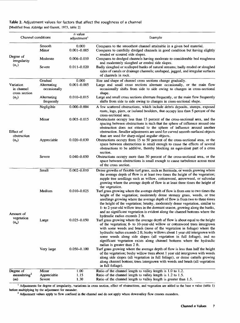
Table 2. Adjustment values for factors that affect the roughness of a channel[Modified from Aldridge and Garrett, 1973, table 2]

Channel conditionsn value

adjustment1 Example

Smooth 0.000 Compares to the smoothest channel attainable in a given bed material. Minor 0.001-0.005 Compares to carefully dredged channels in good condition but having slightly

eroded or scoured side slopes. Moderate 0.006-0.010 Compares to dredged channels having moderate to considerable bed roughness

and moderately sloughed or eroded side slopes. Severe 0.011-0.020 Badly sloughed or scalloped banks of natural streams; badly eroded or sloughed

sides of canals or drainage channels; unshaped, jagged, and irregular surfacesof channels in rock.

Degree of irregularity

Gradual 0.000 Size and shape of channel cross sections change gradually.Variation Alternating 0.001-0.005 Large and small cross sections alternate occasionally, or the main flow

in channel occasionally occasionally shifts from side to side owing to changes in cross-sectionalcross section shape.(«2) Alternating 0.010-0.015 Large and small cross sections alternate frequently, or the main flow frequently

frequently shifts from side to side owing to changes in cross-sectional shape.Negligible 0.000-0.004 A few scattered obstructions, which include debris deposits, stumps, exposed

roots, logs, piers, or isolated boulders, that occupy less than 5 percent of the cross-sectional area.

Minor 0.005-0.015 Obstructions occupy less than 15 percent of the cross-sectional area, and thespacing between obstructions is such that the sphere of influence around one obstruction does not extend to the sphere of influence around another

Effect of obstruction. Smaller adjustments are used for curved smooth-surfaced objects obstruction than are used for sharp-edged angular objects.(«3) Appreciable 0.020-0.030 Obstructions occupy from 15 to 50 percent of the cross-sectional area, or the

space between obstructions is small enough to cause the effects of several obstructions to be additive, thereby blocking an equivalent part of a cross section.

Severe 0.040-0.050 Obstructions occupy more than 50 percent of the cross-sectional area, or thespace between obstructions is small enough to cause turbulence across most of the cross section.

Small 0.002-0.010 Dense growths of flexible turf grass, such as Bermuda, or weeds growing wherethe average depth of flow is at least two times the height of the vegetation; supple tree seedlings such as willow, cottonwood, arrow weed, or saltcedar growing where the average depth of flow is at least three times the height of the vegetation.

Medium 0.010-0.025 Turf grass growing where the average depth of flow is from one to two times theheight of the vegetation; moderately dense stemmy grass, weeds, or tree seedlings growing where the average depth of flow is from two to three times the height of the vegetation; brushy, moderately dense vegetation, similar to 1- to 2-year-old willow trees in the dormant season, growing along the banks, and no significant vegetation is evident along the channel bottoms where the hydraulic radius exceeds 2 ft.

Large 0.025-0.050 Turf grass growing where the average depth of flow is about equal to the heightof the vegetation; 8- to 10-year-old willow or cottonwood trees intergrown with some weeds and brush (none of the vegetation in foliage) where the hydraulic radius exceeds 2 ft; bushy willows about 1 year old intergrown with some weeds along side slopes (all vegetation in full foliage), and no significant vegetation exists along channel bottoms where the hydraulic radius is greater than 2 ft.

Very large 0.050-0.100 Turf grass growing where the average depth of flow is less than half the heightof the vegetation; bushy willow trees about 1 year old intergrown with weeds along side slopes (all vegetation in full foliage), or dense cattails growing along channel bottom; trees intergrown with weeds and brush (all vegetation in full foliage).

Amount of vegetation

Degree of meandering2 (m)

MinorAppreciableSevere

1.00 Ratio of the channel length to valley length is 1.0 to 1.2.1.15 Ratio of the channel length to valley length is 1.2 to 1.5.1.30 Ratio of the channel length to valley length is greater than 1.5.

1 Adjustments for degree of irregularity, variations in cross section, effect of obstructions, and vegetation are added to the base n value (table 1) before multiplying by the adjustment for meander.

2 Adjustment values apply to flow confined in the channel and do not apply where downvalley flow crosses meanders.

Channel n Values

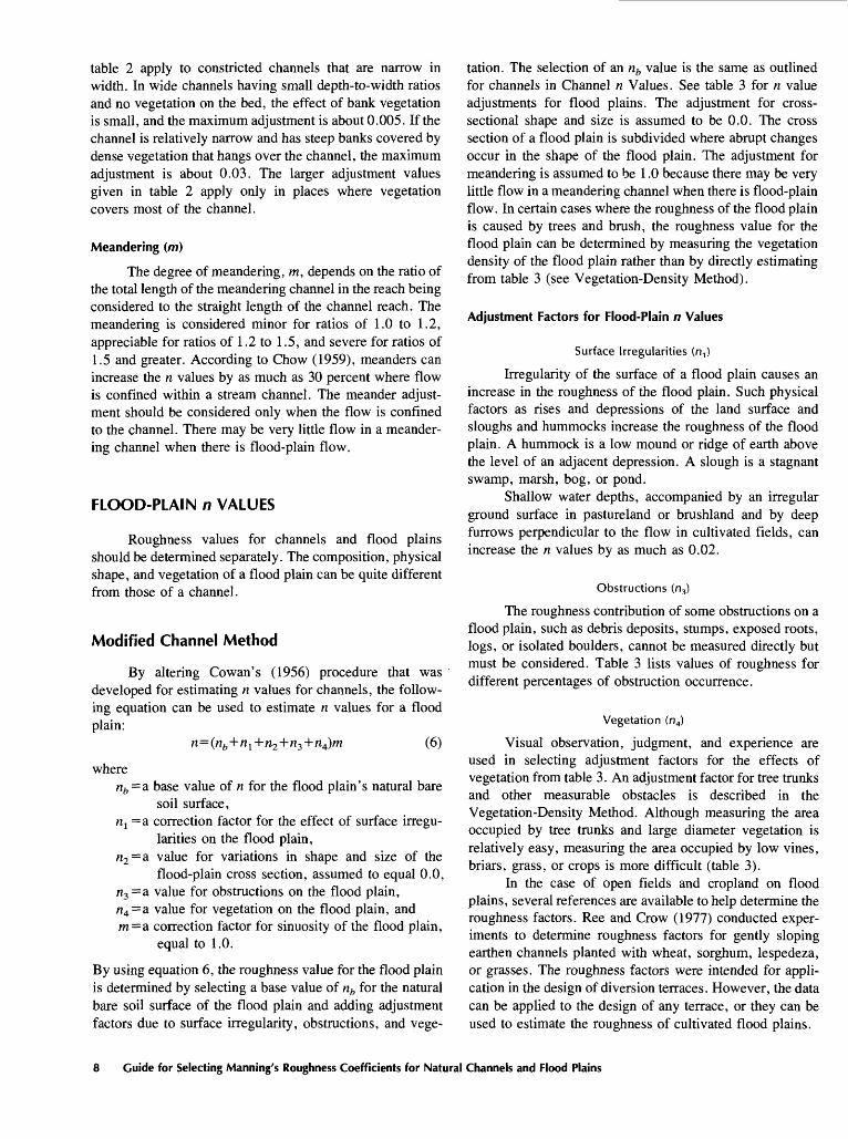
table 2 apply to constricted channels that are narrow in width. In wide channels having small depth-to-width ratios and no vegetation on the bed, the effect of bank vegetation is small, and the maximum adjustment is about 0.005. If the channel is relatively narrow and has steep banks covered by dense vegetation that hangs over the channel, the maximum adjustment is about 0.03. The larger adjustment values given in table 2 apply only in places where vegetation covers most of the channel.

Meandering (m)

The degree of meandering, m, depends on the ratio of the total length of the meandering channel in the reach being considered to the straight length of the channel reach. The meandering is considered minor for ratios of 1.0 to 1.2, appreciable for ratios of 1.2 to 1.5, and severe for ratios of 1.5 and greater. According to Chow (1959), meanders can increase the n values by as much as 30 percent where flow is confined within a stream channel. The meander adjust ment should be considered only when the flow is confined to the channel. There may be very little flow in a meander ing channel when there is flood-plain flow.

FLOOD-PLAIN n VALUES

Roughness values for channels and flood plains should be determined separately. The composition, physical shape, and vegetation of a flood plain can be quite different from those of a channel.

Modified Channel Method

By altering Cowan's (1956) procedure that was developed for estimating n values for channels, the follow ing equation can be used to estimate n values for a flood plain:

n=(nb +n l +n2 +n3 +n4)m (6)

wherenb =a base value of n for the flood plain's natural bare

soil surface,n l =a correction factor for the effect of surface irregu

larities on the flood plain,n2 = a value for variations in shape and size of the

flood-plain cross section, assumed to equal 0.0, n3 =a value for obstructions on the flood plain, n4 =a value for vegetation on the flood plain, and m = a correction factor for sinuosity of the flood plain,

equal to 1.0.

By using equation 6, the roughness value for the flood plain is determined by selecting a base value of nb for the natural bare soil surface of the flood plain and adding adjustment factors due to surface irregularity, obstructions, and vege

tation. The selection of an nb value is the same as outlined for channels in Channel n Values. See table 3 for n value adjustments for flood plains. The adjustment for cross- sectional shape and size is assumed to be 0.0. The cross section of a flood plain is subdivided where abrupt changes occur in the shape of the flood plain. The adjustment for meandering is assumed to be 1.0 because there may be very little flow in a meandering channel when there is flood-plain flow. In certain cases where the roughness of the flood plain is caused by trees and brush, the roughness value for the flood plain can be determined by measuring the vegetation density of the flood plain rather than by directly estimating from table 3 (see Vegetation-Density Method).

Adjustment Factors for Flood-Plain n Values

Surface Irregularities (n.,)

Irregularity of the surface of a flood plain causes an increase in the roughness of the flood plain. Such physical factors as rises and depressions of the land surface and sloughs and hummocks increase the roughness of the flood plain. A hummock is a low mound or ridge of earth above the level of an adjacent depression. A slough is a stagnant swamp, marsh, bog, or pond.

Shallow water depths, accompanied by an irregular ground surface in pastureland or brushland and by deep furrows perpendicular to the flow in cultivated fields, can increase the n values by as much as 0.02.

Obstructions (n3)

The roughness contribution of some obstructions on a flood plain, such as debris deposits, stumps, exposed roots, logs, or isolated boulders, cannot be measured directly but must be considered. Table 3 lists values of roughness for different percentages of obstruction occurrence.

Vegetation (n4)

Visual observation, judgment, and experience are used in selecting adjustment factors for the effects of vegetation from table 3. An adjustment factor for tree trunks and other measurable obstacles is described in the Vegetation-Density Method. Although measuring the area occupied by tree trunks and large diameter vegetation is relatively easy, measuring the area occupied by low vines, briars, grass, or crops is more difficult (table 3).

In the case of open fields and cropland on flood plains, several references are available to help determine the roughness factors. Ree and Crow (1977) conducted exper iments to determine roughness factors for gently sloping earthen channels planted with wheat, sorghum, lespedeza, or grasses. The roughness factors were intended for appli cation in the design of diversion terraces. However, the data can be applied to the design of any terrace, or they can be used to estimate the roughness of cultivated flood plains.


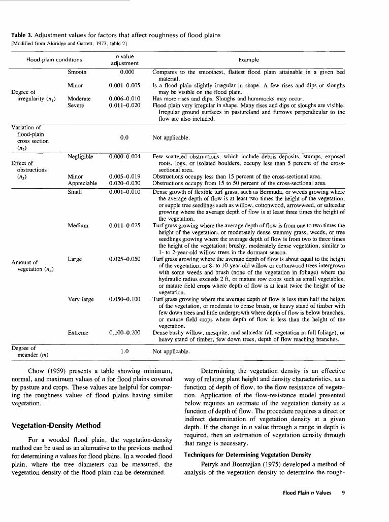
Table 3. Adjustment values for factors that affect roughness of flood plains [Modified from Aldridge and Garrett, 1973, table 2]

Flood-plain conditions

Smooth

Minor Degree of

irregularity (n t ) Moderate Severe

Variation of flood-plain cross section ("2)

Negligible Effect of

obstructions (n3) Minor

AppreciableSmall

Medium

Amount of vegetation («4)

Very large

Extreme

Degree of meander (ni)

n value adjustment

0.000

0.001-0.005

0.006-0.010 0.011-0.020

0.0

0.000-0.004

0.005-0.019 0.020-0.0300.001-0.010

0.011-0.025

0.025-0.050

0.050-0.100

0.100-0.200

1.0

Example

Compares to the smoothest, flattest flood plain attainable in a given bed material.

Is a flood plain slightly irregular in shape. A few rises and dips or sloughs may be visible on the flood plain.

Has more rises and dips. Sloughs and hummocks may occur. Flood plain very irregular in shape. Many rises and dips or sloughs are visible.

Irregular ground surfaces in pastureland and furrows perpendicular to the flow are also included.

Not applicable.

Few scattered obstructions, which include debris deposits, stumps, exposed roots, logs, or isolated boulders, occupy less than 5 percent of the cross- sectional area.

Obstructions occupy less than 15 percent of the cross-sectional area. Obstructions occupy from 15 to 50 percent of the cross-sectional area.Dense growth of flexible turf grass, such as Bermuda, or weeds growing where

the average depth of flow is at least two times the height of the vegetation, or supple tree seedlings such as willow, cottonwood, arrowweed, or saltcedar growing where the average depth of flow is at least three times the height of the vegetation.

Turf grass growing where the average depth of flow is from one to two times the height of the vegetation, or moderately dense stemmy grass, weeds, or tree seedlings growing where the average depth of flow is from two to three times the height of the vegetation; brushy, moderately dense vegetation, similar to 1- to 2-year-old willow trees in the dormant season.

Turf grass growing where the average depth of flow is about equal to the height of the vegetation, or 8- to 10-year-old willow or cottonwood trees intergrown with some weeds and brush (none of the vegetation in foliage) where the hydraulic radius exceeds 2 ft, or mature row crops such as small vegetables, or mature field crops where depth of flow is at least twice the height of the vegetation.

Turf grass growing where the average depth of flow is less than half the height of the vegetation, or moderate to dense brush, or heavy stand of timber with few down trees and little undergrowth where depth of flow is below branches, or mature field crops where depth of flow is less than the height of the vegetation.

Dense bushy willow, mesquite, and saltcedar (all vegetation in full foliage), or heavy stand of timber, few down trees, depth of flow reaching branches.

Not applicable.

Chow (1959) presents a table showing minimum, normal, and maximum values of n for flood plains covered by pasture and crops. These values are helpful for compar ing the roughness values of flood plains having similar vegetation.

Vegetation-Density Method

For a wooded flood plain, the vegetation-density method can be used as an alternative to the previous method for determining n values for flood plains. In a wooded flood plain, where the tree diameters can be measured, the vegetation density of the flood plain can be determined.

Determining the vegetation density is an effective way of relating plant height and density characteristics, as a function of depth of flow, to the flow resistance of vegeta tion. Application of the flow-resistance model presented below requires an estimate of the vegetation density as a function of depth of flow. The procedure requires a direct or indirect determination of vegetation density at a given depth. If the change in n value through a range in depth is required, then an estimation of vegetation density through that range is necessary.

Techniques for Determining Vegetation Density

Petryk and Bosmajian (1975) developed a method of analysis of the vegetation density to determine the rough-

Flood Plain n Values

ness coefficient for a densely vegetated flood plain. By summing the forces in the longitudinal direction of a reach and substituting in the Manning's formula, they developed the following equation:

16

n=nQ - (7)

wheren0 = Manning's boundary-roughness coefficient, exclud

ing the effect of the vegetation (a base n), C* =the effective-drag coefficient for the vegetation in

the direction of flow, 2A,=the total frontal area of vegetation blocking the

flow in the reach, in square feet, g=the gravitational constant, in feet per square sec

ond,A=the cross-sectional area of flow, in square feet, L=the length of channel reach being considered, in

feet, and fl=the hydraulic radius, in feet.

Equation 7 gives the n value in terms of the boundary roughness, «0 , the hydraulic radius, R, the effective-drag coefficient, C*, and the vegetation characteristics, SA/AL. The vegetation density, Vegd, in the cross section is represented by

(8)

The boundary roughness, n0 , can be determined from the follpwing equation:

(9)

The definition of the roughness factors nb and nl through «3 are the same as those in equation 6 and are determined by using table 3. The «4 ' factor, which could not be measured directly in the Vegd term, is for vegetation, such as brush and grass, on the surface of the flood plain. The n/ factor is defined in the small to medium range in table 3 because the tree canopy will prohibit a dense undergrowth in a densely wooded area.

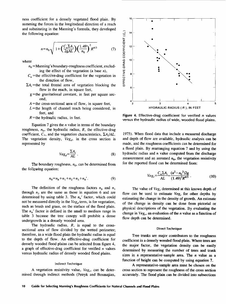
The hydraulic radius, R, is equal to the cross- sectional area of flow divided by the wetted perimeter; therefore, in a wide flood plain the hydraulic radius is equal to the depth of flow. An effective-drag coefficient for densely wooded flood plains can be selected from figure 4, a graph of effective-drag coefficient for verified n values versus hydraulic radius of densely wooded flood plains.

Indirect Technique

A vegetation resistivity value, Vegr, can be deter mined through indirect methods (Petryk and Bosmajian,

O14 -

O 12

10

3 4

HYDRAULIC RADIUS ( R ), IN FEET

Figure 4. Effective-drag coefficient for verified n values versus the hydraulic radius of wide, wooded flood plains.

1975). When flood data that include a measured discharge and depth of flow are available, hydraulic analysis can be made, and the roughness coefficients can be determined for a flood plain. By rearranging equation 7 and by using the hydraulic radius and n value computed from the discharge measurement and an assumed WQ, the vegetation resistivity for the reported flood can be determined from:

VegrAL d.49)2/^3 ' (10)

The value of Vegr determined at this known depth of flow can be used to estimate Vegr for other depths by estimating the change in the density of growth. An estimate of the change in density can be done from pictorial or physical descriptions of the vegetation. By evaluating the change in Vegr, an evaluation of the n value as a function of flow depth can be determined.

Direct Technique

Tree trunks are major contributors to the roughness coefficient in a densely wooded flood plain. Where trees are the major factor, the vegetation density can be easily determined by measuring the number of trees and trunk sizes in a representative-sample area. The n value as a function of height can be computed by using equation 7.

A representative-sample area must be chosen on the cross section to represent the roughness of the cross section accurately. The flood plain can be divided into subsections


on the basis of geometric and (or) roughness differences in the cross section. The vegetation density is determined for each subsection.

The sampling area must be representative of the roughness coefficient of the cross section. By closely examining the cross section in the field, a representative- sample area can be chosen. Another way to more accurately determine the roughness coefficient is to select several representative areas and compare the results. Cross sections should be divided into subsections when changes in rough ness properties occur.

All of the trees, including vines, in the sampling area must be counted, and the diameters must be measured to the nearest 0.1 ft. Each tree diameter is measured to give an average diameter for the expected flow depth of the sample area.

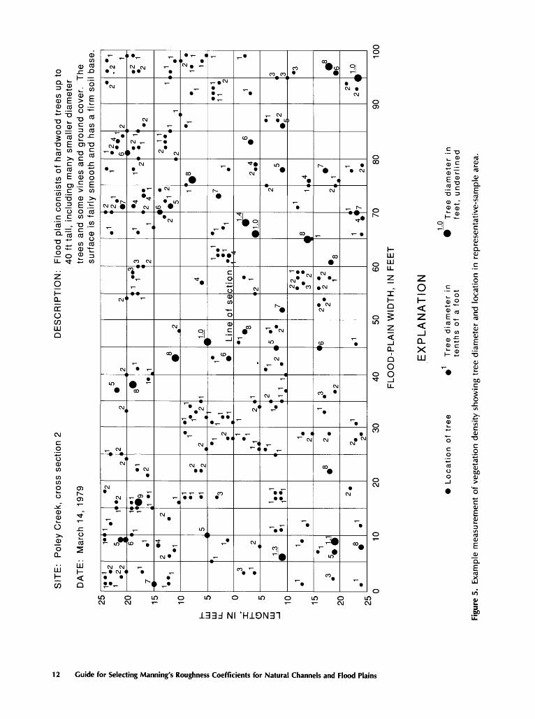
Determining the area occupied by trees within the sampling area is not difficult. A sampling area 100 ft along the cross section by 50 ft in the flow direction is adequate to determine the vegetation density of an area when the sample area is representative of the flood plain. A 100-ft tape is stretched out perpendicular to the flow direction in the sample area. Every tree within 25 ft along either side of the 100-ft tape is counted. The position of the tree is plotted on a grid system by measuring the distance to each tree from the center line along the 100-ft tape, and the diameter of the tree is recorded on the grid system (see fig. 5).

The area, SA,-, occupied by trees in the sampling area can be computed from the number of trees, their diameter, and the depth of flow in the flood plain. Once the vegetation area, XA,-, is determined, the vegetation density can be computed by using equation 8, and the n value for the subsection can be determined by using equation 7 and appropriate values for n0 , R, and C*.

Equation 8 can be simplified to

.Vegd= =

AL

h

hwl(11)

where 2/V/,-=the summation of number of trees multiplied by

tree diameter, in feet, h= height of water on flood plain, in feet, w= width of sample area, in feet, and /=length of sample area, in feet.

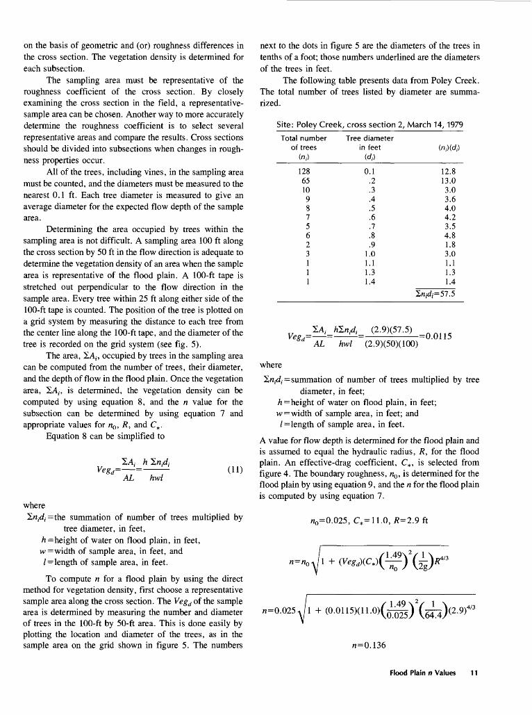
To compute n for a flood plain by using the direct method for vegetation density, first choose a representative sample area along the cross section. The Vegd of the sample area is determined by measuring the number and diameter of trees in the 100-ft by 50-ft area. This is done easily by plotting the location and diameter of the trees, as in the sample area on the grid shown in figure 5. The numbers

next to the dots in figure 5 are the diameters of the trees in tenths of a foot; those numbers underlined are the diameters of the trees in feet.

The following table presents data from Poley Creek. The total number of trees listed by diameter are summa rized.

Site: Poley Creek, cross section 2, March 14,1979

Total number of trees

128 65109875623111

Tree diameter in feet

0.1.2.3.4.5.6.7.8.9

1.01.11.31.4

< ,« 12.8 13.03.03.64.04.23.54.81.83.01.11.31.4

where

Vegd=^='-^Z= (2 ' 9)(57 - 5) =0.0115 AL hwl (2.9)(50)(100)

, := summation of number of trees multiplied by treediameter, in feet;

h = height of water on flood plain, in feet; w= width of sample area, in feet; and /=length of sample area, in feet.

A value for flow depth is determined for the flood plain and is assumed to equal the hydraulic radius, R, for the flood plain. An effective-drag coefficient, C*, is selected from figure 4. The boundary roughness, n0 , is determined for the flood plain by using equation 9, and the n for the flood plain is computed by using equation 7.

n0=0.025, C*=11.0, R=2.9 ft

n=n0

n=0.025 l + (0.01 15)(11.149\ 2 /1

n=0.136

Flood Plain n Values 11

SIT

E:

Pole

y C

reek

, cr

oss

se

ctio

n 2

DA

TE

: M

arc

h 1

4, 1

979

8- 3> 1 3 ere 3 i 70 § « i p o i o i' v> s> z s* sL o i" 2. i Tl I o Si.

25 20 15 10

S3

5U

JL

L -

0

1- 0

5Z

°

UJ

10 15 20 25

DE

SC

RIP

TIO

N:

Flo

od p

lain

consi

sts

of h

ard

wood t

rees

up t

o 40

ft

tall,

in

clu

din

g m

any

smalle

r d

iam

ete

r tr

ees

and

som

e vi

nes

and

gro

un

d c

ove

r.

The

su

rface

is

fairly

sm

oo

th a

nd h

as a

firm

soil

base

.1*

*1

*2

1 2

*.

2

.17

-

' ,

i

.3

.1

1

3 1

1«<

-£ 6

<

.1

2 *

4

1

<

*1

1. 2

1.3

1.

*1

.* .*

'1.1

1<

(1

1< 1

1' t

2

5 .1 1

.1

.1

2

' 2

' 1

' 9

,1 !

.1

1 1

1 *3

1..

1 1«

*1 2.

1 2J

1

2 .2

2

4

8

,1 ,2

1*

2 *1 .2

1

i/1

1 1

1.

2.

2.

2. 2

«

2

1

1iV

2 <

»1

'1

.1

^ 1 1

2 <

1.' i

1

.<

,5 8*

1

1«

>1 1 2 '1.1

1,

.3 2

,2 .1

,1

1* 6

*1

2 <

i

4

.2

1.0

z^-

Lin

e"X 5

'I

2

>6 .1

2

i i 1

of

se

(

,7 2*2-

i 1

««3

> 1

< c

4

ctio

n 2

1

.22.J

3 2

" *.2

,3 I

2 1 1

&-

H s

1 <

' 4

.1

( 1

4

2

*1 *1

1.4

L

O

^H 1 : v

2'2

.1

7 4 IP

^ 4

1

>6

. r2 r 7

2(

.1

1,

2,

,1 '7

'V

1

1 2..4 .5

»4,7

, 1

f

.1 2*

^2

4 6'<

1

^7

' *1

'

2 1

1 <

'2

.6

2 i 2 .11

*1

1

<2

2 1

,

1

11

*2

1

1

2«

-4

*1

-

2 1 1

2

2

1

"1

.1

^7

i«

1 1*

1 1

3 i 3 3

6 (1

J

1020

30

40

50

60

FLO

OD

-PLA

IN W

IDT

H,

IN F

EE

T

7080

9010

0

L

oca

tio

n

of

tree

EX

PLA

NA

TIO

N

Tre

e dia

mete

r in

te

nth

s of

a

foot

1.0

Tre

e d

iam

ete

r in

fe

et, underlin

ed

Figu

re 5

. E

xam

ple

mea

sure

men

t o

f ve

geta

tion

dens

ity s

how

ing

tree

dia

met

er a

nd l

ocat

ion

in r

epre

sent

ativ

e-sa

mpl

e ar

ea.

PHOTOGRAPHS OF FLOOD PLAINS

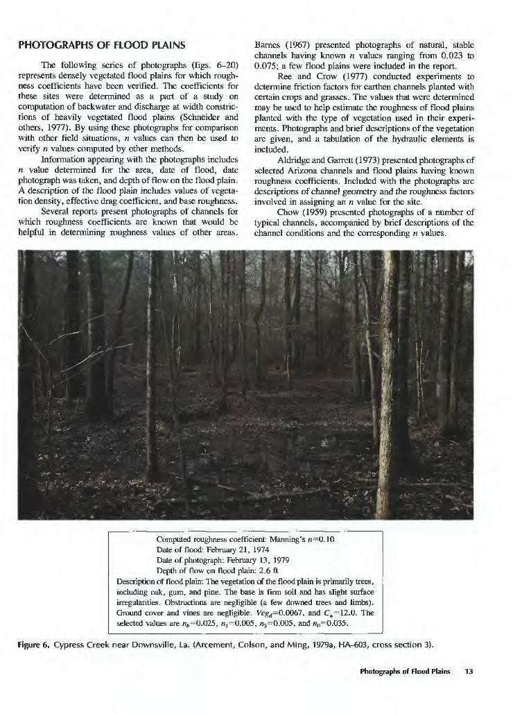
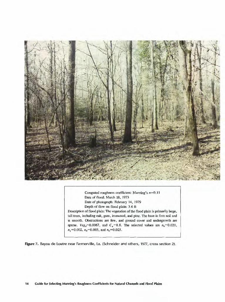
The following series of photographs (figs. 6-20) represents densely vegetated flood plains for which rough ness coefficients have been verified. The coefficients for these sites were determined as a part of a study on computation of backwater and discharge at width constric tions of heavily vegetated flood plains (Schneider and others, 1977). By using these photographs for comparison with other field situations, n values can then be used to verify n values computed by other methods.

Information appearing with the photographs includes n value determined for the area, date of flood, date photograph was taken, and depth of flow on the flood plain. A description of the flood plain includes values of vegeta tion density, effective drag coefficient, and base roughness.

Several reports present photographs of channels for which roughness coefficients are known that would be helpful in determining roughness values of other areas.

Barnes (1967) presented photographs of natural, stable channels having known n values ranging from 0.023 to 0.075; a few flood plains were included in the report.

Ree and Crow (1977) conducted experiments to determine friction factors for earthen channels planted with certain crops and grasses. The values that were determined may be used to help estimate the roughness of flood plains planted with the type of vegetation used in their experi ments. Photographs and brief descriptions of the vegetation are given, and a tabulation of the hydraulic elements is included.

Aldridge and Garrett (1973) presented photographs of selected Arizona channels and flood plains having known roughness coefficients. Included with the photographs are descriptions of channel geometry and the roughness factors involved in assigning an n value for the site.

Chow (1959) presented photographs of a number of typical channels, accompanied by brief descriptions of the channel conditions and the corresponding n values.

Computed roughness coefficient: Manning's n=0.10Date of flood: February 21, 1974Date of photograph: February 13, 1979Depth of flow on flood plain: 2.6 ft

Description of flood plain: The vegetation of the flood plain is primarily trees, including oak, gum, and pine. The base is firm soil and has slight surface irregularities. Obstructions are negligible (a few downed trees and limbs). Ground cover and vines are negligible. Vegd=0.0067, and C,,=12.0. The selected values are nt=0.025, nÔ.005, n3 =0.005, and n0=0.035.

Figure 6. Cypress Creek near Downsville, La. (Arcement, Colson, and Ming, 1979a, HA-603, cross section 3).

Photographs of Flood Plains 13

Computed roughness coefficient: Manning's n=0.llDate of flood: March 18, 1973Date of photograph: February 14, 1979Depth of flow on flood plain: 3.6 ft

Description of flood plain: The vegetation of the flood plain is primarily large, tall trees, including oak, gum, ironwood, and pine. The base is firm soil and is smooth. Obstructions are few, and ground cover and undergrowth are sparse. Vegd=0.0067, and C_=8.8. The selected values are nfc=0.020, n, =0.002, n3 =0.003, and «0=0.025.

Figure 7. Bayou de Loutre near Farmerville, La. (Schneider and others, 1977, cross section 2).


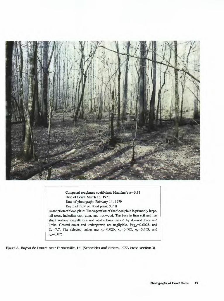
Computed roughness coefficient: Manning's n=0.11Date of flood: March 18, 1973Date of photograph: February 14, 1979Depth of flow on flood plain: 3.7 ft

Description of flood plain: The vegetation of the flood plain is primarily large, tall trees, including oak, gum, and ironwood. The base is firm soil and has slight surface irregularities and obstructions caused by downed trees and limbs. Ground cover and undergrowth are negligible. Vegd=0.0075, and C.=7.7. The selected values are nfc =0.020, ^=0.002, n3=0.003, and 710=0.025.



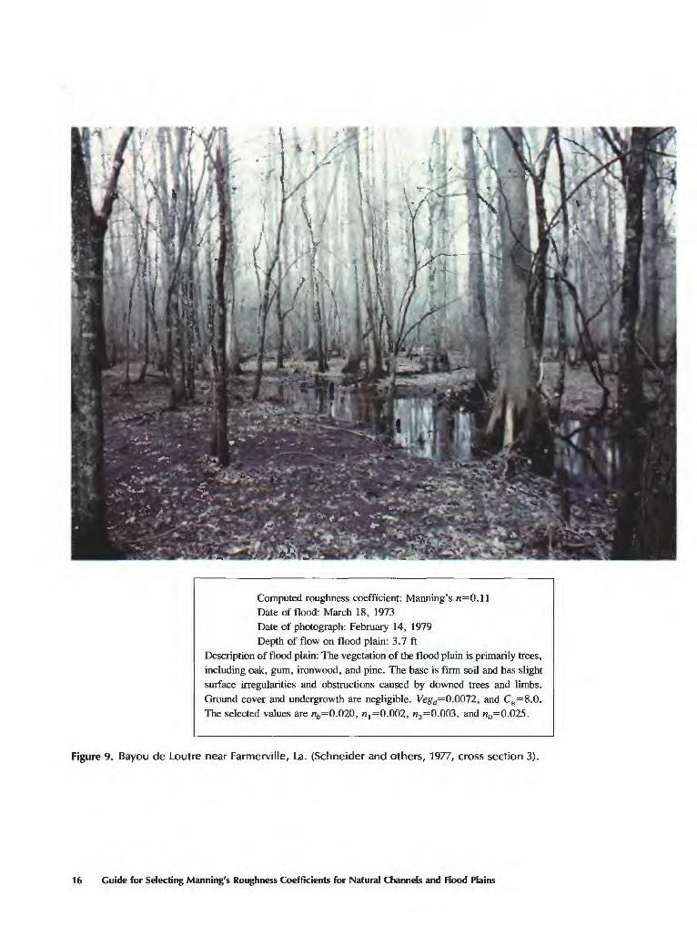
Computed roughness coefficient: Manning's n=0.11Date of flood: March 18, 1973Date of photograph: February 14, 1979Depth of flow on flood plain: 3.7 ft

Description of flood plain: The vegetation of the flood plain is primarily trees, including oak, gum, ironwood, and pine. The base is firm soil and has slight surface irregularities and obstructions caused by downed trees and limbs. Ground cover and undergrowth are negligible. Vegd=0.0072, and C_=8.0. The selected values are nfc=0.020, nÔ.002, n3 =0.003, and n0=0.025.



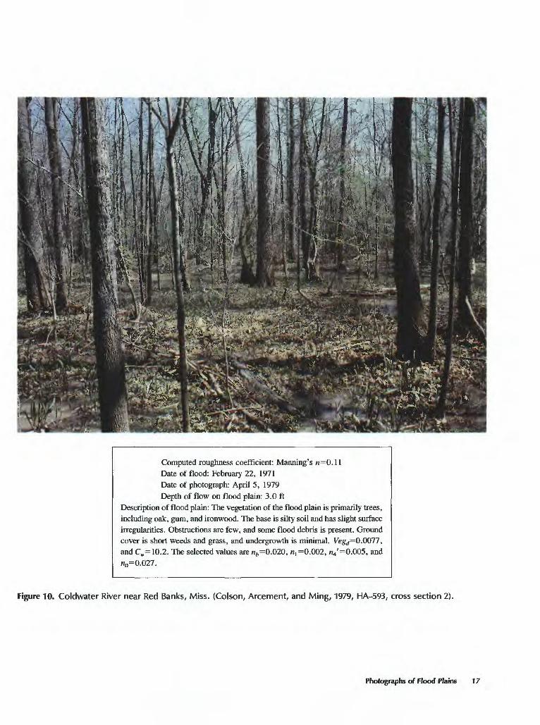
Computed roughness coefficient: Manning's n=0.11Date of flood: February 22, 1971Date of photograph: April 5, 1979Depth of flow on flood plain: 3.0 ft

Description of flood plain: The vegetation of the flood plain is primarily trees, including oak, gum, and ironwood. The base is silty soil and has slight surface irregularities. Obstructions are few, and some flood debris is present. Ground cover is short weeds and grass, and undergrowth is minimal. Vegd=0.0077, and C»=10.2. The selected values are nfc =0.020, n, =0.002, n4'=0.005, and 7io=0.027.

Figure 10. Coldwater River near Red Banks, Miss. (Colson, Arcement, and Ming, 1979, HA-593, cross section 2).


«w«§n^

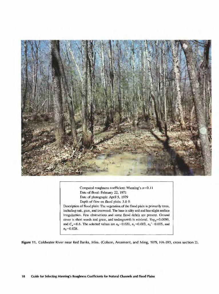
Computed roughness coefficient: Manning's n=0.11Date of flood: February 22, 1971Date of photograph: April 5, 1979Depth of flow on flood plain: 3.0 ft

Description of flood plain: The vegetation of the flood plain is primarily trees, including oak, gum, and ironwood. The base is silty soil and has slight surface irregularities. Few obstructions and some flood debris are present. Ground cover is short weeds and grass, and undergrowth is minimal. Vegd=0.0090, and C,=8.6. The selected values are nfc =0.020, n, =0.003, n4'=0.005, and no=0.028.

Figure 11. Coldwater River near Red Banks, Miss. (Colson, Arcement, and Ming, 1979, HA-593, cross section 2).


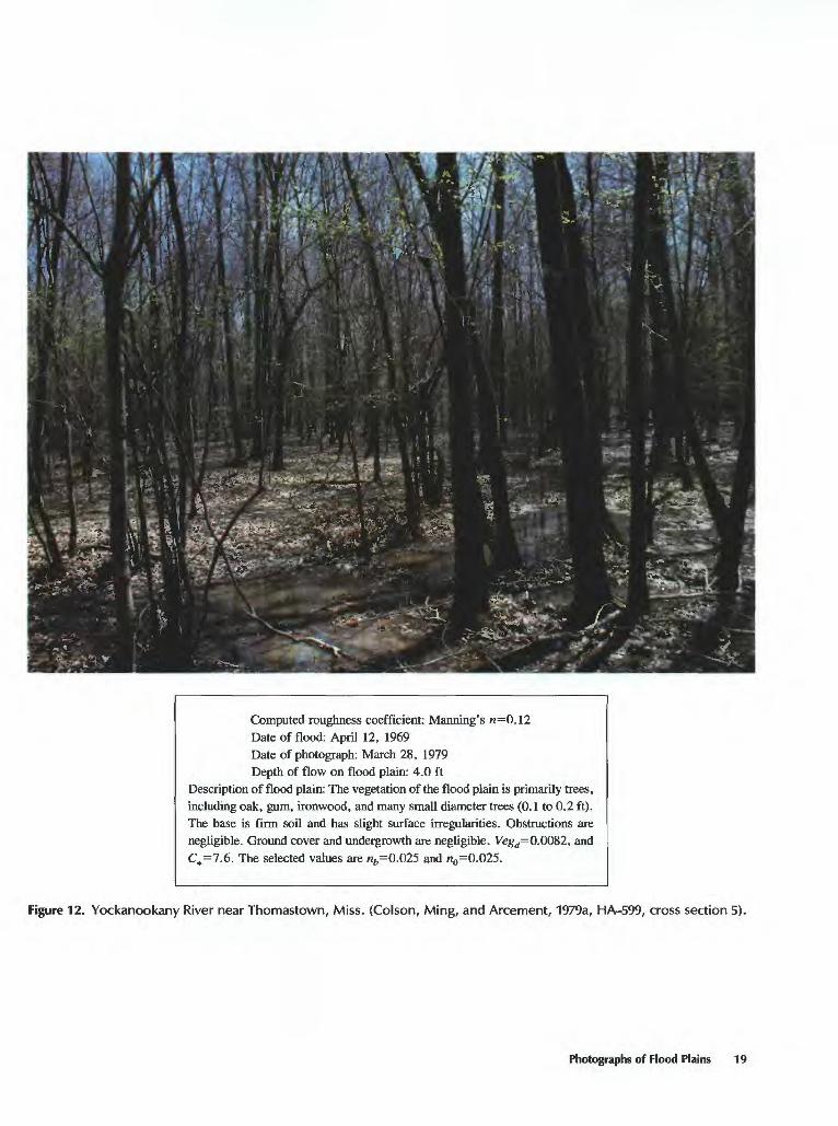
Computed roughness coefficient: Manning's n=0.12Date of flood: April 12, 1969Date of photograph: March 28, 1979Depth of flow on flood plain: 4.0 ft

Description of flood plain: The vegetation of the flood plain is primarily trees, including oak, gum, ironwood, and many small diameter trees (0.1 to 0.2 ft). The base is firm soil and has slight surface irregularities. Obstructions are negligible. Ground cover and undergrowth are negligible. Vegd=O.OOS2, and Cf=7.6. The selected values are nfc =0.025 and rto=0.025.

Figure 12. Yockanookany River near Thomastown, Miss. (Colson, Ming, and Arcement, 1979a, HA-599, cross section 5).


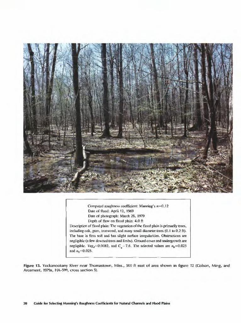
Computed roughness coefficient: Manning's «=0.12Date of flood: April 12, 1969Date of photograph: March 28, 1979Depth of flow on flood plain: 4.0 ft

Description of flood plain: The vegetation of the flood plain is primarily trees, including oak, gum, ironwood, and many small diameter trees (0.1 to 0.2 ft). The base is firm soil and has slight surface irregularities. Obstructions are negligible (a few downed trees and limbs). Ground cover and undergrowth are negligible. Vegd=O.QOS2, and 0^=7.6. The selected values are «6=0.025 and n0=0.025.

Figure 13. Yockanookany River near Thomastown, Miss., 500 ft east of area shown in figure 12 (Colson, Ming, and Arcement, 1979a, HA-599, cross section 5).


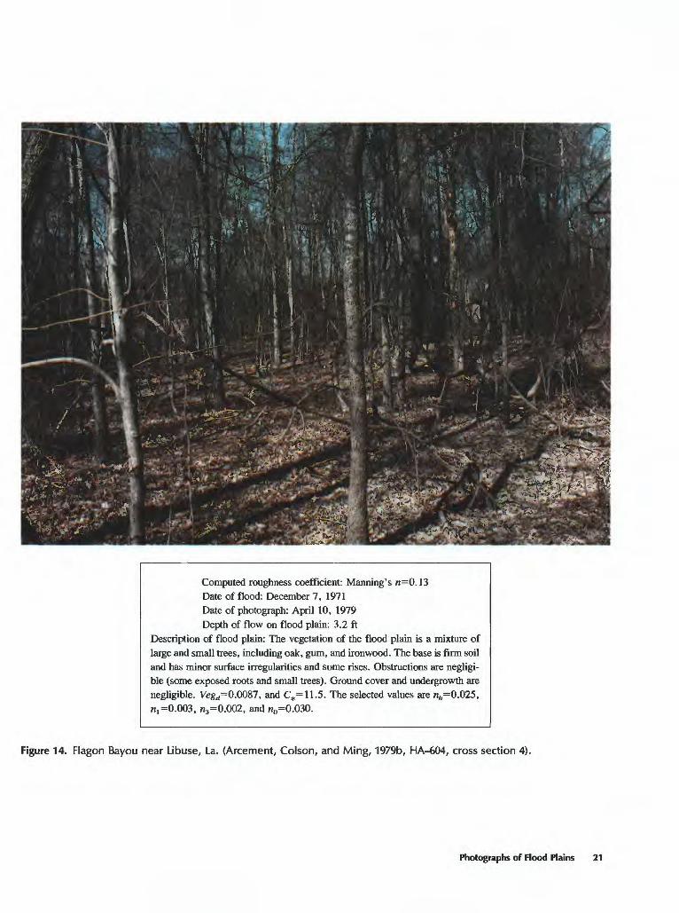
Computed roughness coefficient: Manning's n=0.13Date of flood: December?, 1971Date of photograph: April 10, 1979Depth of flow on flood plain: 3.2 ft

Description of flood plain: The vegetation of the flood plain is a mixture of large and small trees, including oak, gum, and ironwood. The base is firm soil and has minor surface irregularities and some rises. Obstructions are negligi ble (some exposed roots and small trees). Ground cover and undergrowth are negligible. Ve&,=0.0087, and C»=11.5. The selected values are nfc=0.025, n, =0.003, n3 =0.002, and w0=0.030.

Figure 14. Flagon Bayou near Libuse, La. (Arcement, Colson, and Ming, 1979b, HA-604, cross section 4).


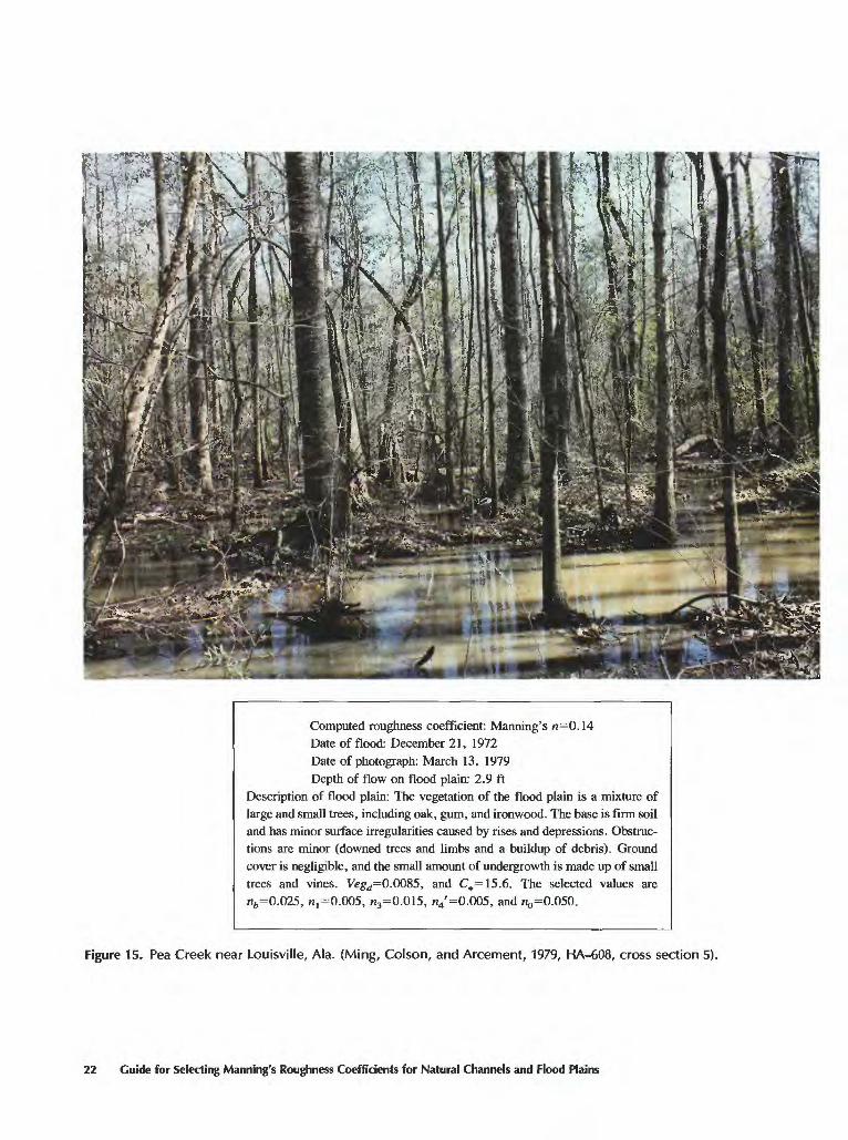
Computed roughness coefficient: Manning's n=0.14Date of flood: December 21, 1972Date of photograph: March 13, 1979Depth of flow on flood plain: 2.9 ft

Description of flood plain: The vegetation of the flood plain is a mixture of large and small trees, including oak, gum, and ironwood. The base is firm soil and has minor surface irregularities caused by rises and depressions. Obstruc tions are minor (downed trees and limbs and a buildup of debris). Ground cover is negligible, and the small amount of undergrowth is made up of small trees and vines. Vegd=0.0085, and C«=15.6. The selected values are nfc =0.025, n, =0.005, n3 =0.015, n4'=0.005, and «0=0.050.

Figure 15. Pea Creek near Louisville, Ala. (Ming, Colson, and Arcement, 1979, HA-608, cross section 5).


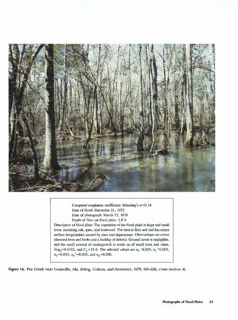
Computed roughness coefficient: Manning's n=0.14Date of flood: December 21, 1972Date of photograph: March 13, 1979Depth of flow on flood plain: 2.8 ft

Description of flood plain: The vegetation of the flood plain is large and small trees, including oak, gum, and ironwood. The base is firm soil and has minor surface irregularities caused by rises and depressions. Obstructions are minor (downed trees and limbs and a buildup of debris). Ground cover is negligible, and the small amount of undergrowth is made up of small trees and vines. Vegd=0.0l02, and C_=15.6. The selected values are nfc =0.025, nÔ.005, n3 =0.015, n4 '=0.005, and n0=0.050.

Figure 16. Pea Creek near Louisville, Ala. (Ming, Colson, and Arcement, 1979, HA-608, cross section 4).


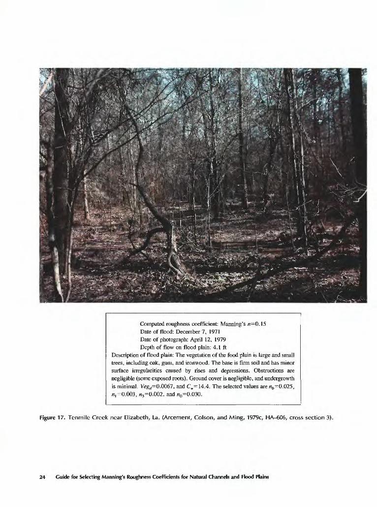
Computed roughness coefficient: Manning's n=0.15Date of flood: December 7, 1971Date of photograph: April 12, 1979Depth of flow on flood plain: 4.1 ft

Description of flood plain: The vegetation of the food plain is large and small trees, including oak, gum, and ironwood. The base is firm soil and has minor surface irregularities caused by rises and depressions. Obstructions are negligible (some exposed roots). Ground cover is negligible, and undergrowth is minimal. Vegd=0.0067, and C^=14.4. The selected values are nfc =0.025, n, =0.003, «3=0.002, and n0=0.030.

Figure 17. Tenmile Creek near Elizabeth, La. (Arcement, Colson, and Ming, 1979c, HA-606, cross section 3).


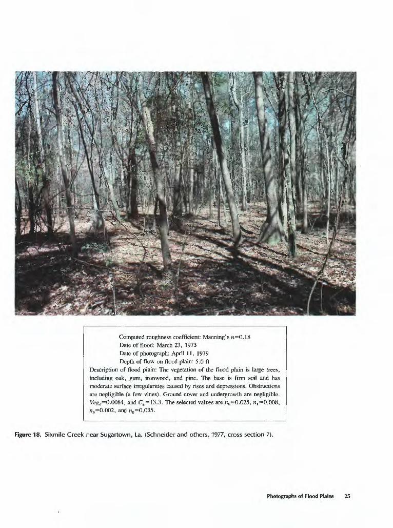
Computed roughness coefficient: Manning's n=0.18Date of flood: March 23, 1973Date of photograph: April 11, 1979Depth of flow on flood plain: 5.0 ft

Description of flood plain: The vegetation of the flood plain is large trees, including oak, gum, ironwood, and pine. The base is firm soil and has moderate surface irregularities caused by rises and depressions. Obstructions are negligible (a few vines). Ground cover and undergrowth are negligible. Vegd=0.0084, and CÎS.3. The selected values are nfc =0.025, n,=0.008, n3 =0.002, and n0=0.035.

Figure 18. Sixmile Creek near Sugartown, La. (Schneider and others, 1977, cross section 7).


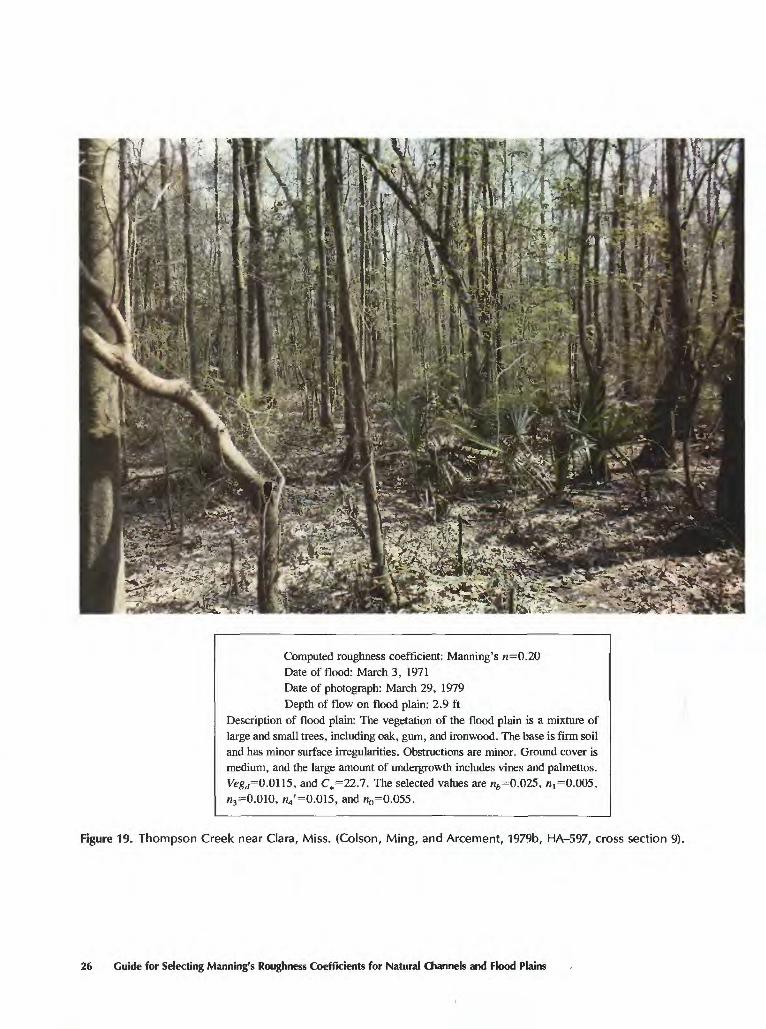
Computed roughness coefficient: Manning's n=0.20Date of flood: March 3, 1971Date of photograph: March 29, 1979Depth of flow on flood plain: 2.9 ft

Description of flood plain: The vegetation of the flood plain is a mixture of large and small trees, including oak, gum, and ironwood. The base is firm soil and has minor surface irregularities. Obstructions are minor. Ground cover is medium, and the large amount of undergrowth includes vines and palmettos. Vegd=0.0ll5, and C,,=22.7. The selected values are nfc =0.025, ni=0.005, n3 =0.010, n4 '=0.015, and n0=0.055.

Figure 19. Thompson Creek near Clara, Miss. (Colson, Ming, and Arcement, 1979b, HA-597, cross section 9).


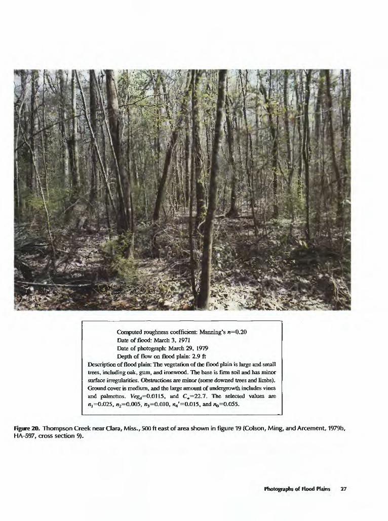
Computed roughness coefficient: Manning's n=0.20Date of flood: March 3, 1971Date of photograph: March 29, 1979Depth of flow on flood plain: 2.9 ft

Description of flood plain: The vegetation of the flood plain is large and small trees, including oak, gum, and ironwood. The base is firm soil and has minor surface irregularities. Obstructions are minor (some downed trees and limbs). Ground cover is medium, and the large amount of undergrowth includes vines and palmettos. Vegd=0.0ll5, and C,=22.7. The selected values are n,=0.025, B2=0.005, «3=0.010, n4'=0.015, and ^=0.055.

Figure 20. Thompson Creek near Clara, Miss., 500 ft east of area shown in figure 19 (Colson, Ming, and Arcement, 1979b, HA-597, cross section 9).


PROCEDURES FOR ASSIGNING n VALUES

When determining n values for a cross section, pans of the procedure apply only to roughness of channels, and other pans apply to roughness of flood plains.

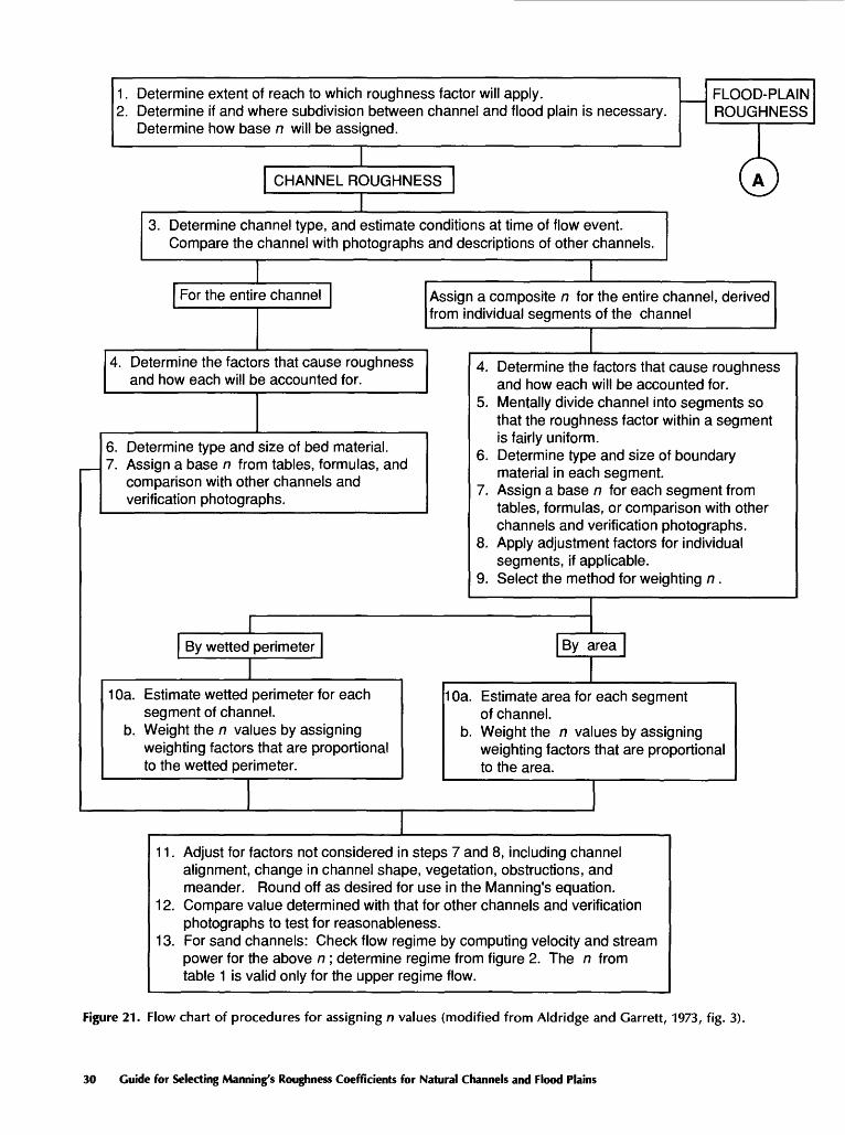
The procedure involves a series of decisions that are based on the interaction of roughness factors. A flow chart (fig. 21) illustrates the steps in the procedure (see Steps for Assigning n values). A form (fig. 22) is provided to help in the computation of the n values. After using the procedure a few times, the user may wish to combine steps or to change the order of the steps. Experienced personnel may perform the entire operation mentally, but the inexperienced user may find the form in figure 22 useful. Steps 3 through 13 apply to channel roughness, and steps 14 through 23 apply to flood-plain roughness. The procedure is adapted from the report by Aldridge and Garrett (1973) but is extended to include assigning n values for flood plains.

Steps for Assigning n Values

Reach Subdivision (Steps 1 and 2)

1. Determine the extent of stream reach to which the roughness factor will apply. Although n may be applied to an individual cross section that is typical of a reach, the roughness in the reach that encompasses the section must be taken into account. When two or more cross sections are being considered, the reach that applies to any one section is considered to extend halfway to the next section. For example, in figure 1, the n value for cross section 1 represents the roughness in reach A, and the n value for cross section 2 represents the roughness in reach B. If the roughness is not uniform throughout the reach being con sidered, n should be assigned for average conditions.

2. If the roughness is not uniform across the width of the cross section, determine where subdivision of the cross section should occur. Determine whether subdivision between channel and flood plain is necessary and whether subdivision of the channel or flood plain is also necessary. If the roughness is not uniform across the width of the channel, determine whether a base n should be assigned to the entire channel cross section or whether a composite n should be derived by weighting values for individual segments of the channel having different amounts of rough ness (see steps 4-10). When the base value is assigned to the entire channel, the channel constitutes the one segment being considered, and steps 5, 8, 9, and 10 do not apply.

Channel Roughness (Steps 3-13)

3. Determine the channel type stable channel, sand channel, or a combination and whether the conditions are

representative of those that may exist during the design event being considered. Look especially for evidence of bed movement and excessive amounts of bank scour. If the conditions do not appear to be the same as those that will exist during the flow event, attempt to visualize the condi tions that will occur. To estimate the possible range in n values, compare the channel with other channels for which n values have been verified or assigned by experienced personnel (see photographs in Barnes, 1967).

4. Determine the factors that cause roughness and how each is to be taken into account. Some factors may be predominant in a particular segment of the channel, or they may affect the entire cross section equally. The manner in which each factor is handled depends on how it combines with other factors. A gently sloping bank may constitute a separate segment of the cross section, whereas a vertical bank may add roughness either to the adjacent segment or to the entire channel. Obstructions, such as debris, may be concentrated in one segment of the channel. Isolated boul ders should be considered as obstructions, but if boulders are scattered over the entire reach, consider them in determining the median particle size of the bed material. Vegetation growing in a distinct segment of the channel may be assigned an n value of its own, whereas roughness caused by vegetation growing only along steep banks or scattered on the channel bottom will be accounted for by means of an adjustment factor that can be applied to either a segment of the channel or to the entire cross section. If a composite n is being derived from segments, the user should continue with step 5; otherwise step 5 should be omitted.

5. Divide the channel width into segments according to roughness. If distinct, parallel banks of material of different particle sizes or of different roughness are present, defining the contact between the types of material is fairly easy (see fig. 1, cross section 2). The dividing line between any two segments should parallel the flow lines in the stream and should be located so as to represent the average contact between types of material. The dividing line must extend through the entire reach, as defined in step 1, although one of the types of bed material may not be present throughout the reach. If a segment contains more than one type of roughness, use an average size of bed material. Where sand is mixed with gravel, cobbles, and boulders throughout a channel, dividing the main channel is imprac tical.

6. Determine the type of material that occupies and bounds each segment of channel and compute the median particle size in each segment by using either method A or B (below). If the Limerinos equation (eq. 5) is used, the size corresponding to the 84th percentile should be used in the computation.

A. If the particles can be separated by screening according to size, small samples of the bed material are


collected at 8 to 12 sites in the segment of the reach. The samples are combined, and the composite sample is passed through screens that divide it into at least five size ranges. Either the volume or weight of material in each range is measured and converted to a percentage of the total.

B. If the material is too large to be screened, a grid system having 50 to 100 intersecting points or nodes per segment is laid out. The width, or intermediate diameter, of each particle that falls directly under a node is measured and recorded. The sizes are grouped into at least five ranges. The number of particles in each range is recorded and converted to a percentage of the total sample.

In the above sampling methods, the size that corre sponds to the 50th percentile (table 1) or the 84th percentile (the Limerinos method) is obtained from a distribution curve derived by plotting particle size versus the percentage of sample smaller than the indicated size. Experienced personnel can make a fairly accurate estimate of the median particle size by inspection of the channel if the range in particle size is small.

7. Determine the base n for each segment of channel by using table 1 or equation 5 or the comparison given in step 3. Chow's (1959) base values (table 1) are for the smoothest condition possible for a given material. The values (table 1) of Benson and Dalrymple (1967) are for a straight, uniform channel of the indicated material and are closer to actual field values than are those of Chow. If a composite n is being derived from segments, proceed with step 8. If n is being assigned for the channel as a whole, proceed to step 11.

8. Add the adjustment factors from table 2 that apply only to individual segments of the channel.

9. Select the basis for weighting n for the channel segments. Wetted perimeter should be used for trapezoidal and V-shaped channels having banks of one material and beds of another material. Wetted perimeter should be used also where the depth across the channel is fairly uniform. Area should be used where the depth varies considerably or where dense brush occupies a large and distinct segment of the channel.

10. Estimate the wetted perimeter or area for each segment and assign a weighting factor to each segment that is proportional to the total wetted perimeter or area. Weight n by multiplying the n for each segment by the assigned weighting factor.

11. Select the adjustment factors from table 2 for conditions that influence n for the entire channel. Do not include adjustment factors for any items used in steps 7 and 8. Consider upstream conditions that may cause a distur bance in the reach being studied. If Chow's (1959) base values are used, the adjustment factors in table 2 may be used directly. If base values are computed from the Limeri nos equation (eq. 5) or are taken from Benson and Dalrym

ple (1967), the adjustment factors should be from one-half to three-fourths as large as those given in table 2. If n is assigned on the basis of a comparison with other streams, the adjustment factors will depend on the relative amounts of roughness in the two streams. Add the adjustment factors to the weighted n values from step 10 to derive the overall n for the channel reach being considered. When a multiply ing factor for meander is used, first add the other adjust ments to the base n. Round off the n value as desired. The value obtained is the composite or overall n for the channel reach selected in step 1. When more than one reach is used, repeat steps 1-13 for each reach.

12. Compare the study reach with photographs of other channels found in Barnes (1967) and Chow (1959) to determine if the final values of n obtained in step 11 appear reasonable.

13. Check the flow regime for all sand channels. Use the n from step 11 in the Manning's equation (eq. 1) to compute the velocity, which is then used to compute stream power. The flow regime is determined from figure 2. The assigned value of n is not reliable unless the stream power is sufficient to cause upper regime flow.

Flood-Plain Roughness (Steps 14-23)

14. As in step 1, the n value selected must be representative of the average conditions of the reach being considered. Determine if the flood-plain conditions are representative of those that may exist during the design event being considered. Compare the flood plain with other flood plains for which n values have been determined (or have been assigned by experienced personnel) to estimate the possible range in n values. Compare with photographs in this guide and in other references.

15. The n value for the flood plain can be determined by using the measurement of vegetation density or resistiv ity. There may be cases where the roughness is determined by a qualitative evaluation of the roughness by using equation 6 and the adjustment factors in table 3. A decision must be made as to which method will be used.

16. If there are abrupt changes in roughness on the flood plain, subdivide the flood-plain cross sections. A representative sampling area is selected for each subarea of the flood plain.

17. Determine the factors that cause roughness and how each is to be taken into account. Such factors as surface irregularities and obstructions can be accounted for in the boundary roughness, whereas vegetation can be accounted for in the boundary roughness or by using the quantitative method.

18. A base value, nb , for the flood plain's bare soil surface must be chosen. A value for nb is chosen from table 1.

Procedures for Assigning n Values 29

1. Determine extent of reach to which roughness factor will apply.2. Determine if and where subdivision between channel and flood plain is necessary.

Determine how base n will be assigned.

FLOOD-PLAIN ROUGHNESS

CHANNEL ROUGHNESS ©3. Determine channel type, and estimate conditions at time of flow event.

Compare the channel with photographs and descriptions of other channels.

For the entire channel Assign a composite n for the entire channel, derived from individual segments of the channel

4. Determine the factors that cause roughness and how each will be accounted for.

6. Determine type and size of bed material.7. Assign a base n from tables, formulas, and

comparison with other channels and verification photographs.

4. Determine the factors that cause roughness and how each will be accounted for.

5. Mentally divide channel into segments so that the roughness factor within a segment is fairly uniform.

6. Determine type and size of boundary material in each segment.

7. Assign a base n for each segment from tables, formulas, or comparison with other channels and verification photographs.

8. Apply adjustment factors for individual segments, if applicable.

9. Select the method for weighting n.

By wetted perimeter

10a. Estimate wetted perimeter for eachsegment of channel,

b. Weight the n values by assigning weighting factors that are proportional to the wetted perimeter.

10a. Estimate area for each segmentof channel.

b. Weight the n values by assigning weighting factors that are proportional to the area.

11

12

Adjust for factors not considered in steps 7 and 8, including channel alignment, change in channel shape, vegetation, obstructions, and meander. Round off as desired for use in the Manning's equation. Compare value determined with that for other channels and verification photographs to test for reasonableness.

13. For sand channels: Check flow regime by computing velocity and stream power for the above n ; determine regime from figure 2. The n from table 1 is valid only for the upper regime flow.

Figure 21. Flow chart of procedures for assigning n values (modified from Aldridge and Garrett, 1973, fig. 3).


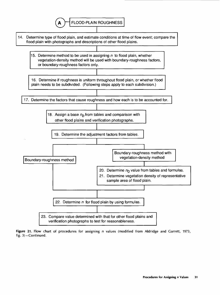
FLOOD-PLAIN ROUGHNESS

14. Determine type of flood plain, and estimate conditions at time of flow event; compare the flood plain with photographs and descriptions of other flood plains.

15. Determine method to be used in assigning n to flood plain, whether vegetation-density method will be used with boundary-roughness factors, or boundary-roughness factors only.

16. Determine if roughness is uniform throughout flood plain, or whether flood plain needs to be subdivided. (Following steps apply to each subdivision.)

17. Determine the factors that cause roughness and how each is to be accounted for.

18. Assign a base n/jfrom tables and comparison with other flood plains and verification photographs.

19. Determine the adjustment factors from tables.

Boundary-roughness method

Boundary-roughness method with vegetation-density method

20. Determine HQ value from tables and formulas.21. Determine vegetation density of representative

sample area of flood plain.

22. Determine n for flood plain by using formulas.

23. Compare value determined with that for other flood plains and verification photographs to test for reasonableness.

Figure 21. Flow chart of procedures for assigning n values (modified from Aldridge and Garrett, 1973, fig. 3) Continued.

Procedures for Assigning n Values 31

19. Select the adjustment factors from table 3 for conditions that influence roughness of the flood-plain sub section.

20. Determine the n0 value by equation 9, by using the adjustment factors selected in step 19. The n4 ' value is the adjustment factor for vegetation not accounted for by the vegetation-density method.

21. The vegetation density of the sampling area is determined by using equation 11 and measuring the cross- sectional area occupied by the trees and undergrowth in the sampling area. An estimate of the depth of flow on the flood plain is necessary to determine the vegetation density and the n value. By measuring two or three sampling areas in a subsection, a more representative value for vegetation density can be determined.

22. The n value for the flood-plain subsection is determined by using equation 6 or 7, depending on which method has been chosen. If the quantitative method is being used, the n value for each subarea of the flood plain is computed by using equation 7 and vegetation-density and boundary-roughness values for each subarea.

23. Compare the study reach with photographs of other flood plains in this report and in other references to determine if the final values of n obtained in step 22 appear to be reasonable.

Examples of Procedures for Determining n Values

A sketch of a hypothetical channel and flood plain is shown in figure 1, and procedures for determining n values are outlined in table 4. The channel and flood plain together are divided into three separate reaches (A, B, C), and each reach has a cross section (1, 2, 3). The shape of each cross section is shown in figure 1.

In cross section 1, the flow is confined to the channel. The channel is composed of firm soil, and no subdivision of the channel is necessary. Steps 1 through 13, in Steps for Assigning n Values, are used in the computation of n for cross section 1. These steps apply only to channel condi tions.

Flow in cross section 2 is also confined to the channel, which is composed of three distinct parallel bands of (1) bedrock, (2) sand, and (3) gravel and cobbles. The n value for each segment is determined and a composite n for the channel is computed by weighting each segment n value by the wetted perimeter. Again, steps 1 through 13 are used in the computation of n for cross section 2.

The flow in cross section 3 is channel and flood-plain flow. The cross section is divided into three subsections. Subsection 1 is flood-plain flow through woods, subsection

2 is channel flow, and subsection 3 is flood-plain flow through a cotton field.

In subsection 1, the flood plain is made up of dense woods having little undergrowth. The procedure using the vegetation density of the woods is used to determine the n value for the flood plain. The vegetation density is deter mined from a representative-sample area of the wooded flood plain. A boundary roughness, n0 , is determined from equation 9 and the n value is determined by using equation 7. Steps 14 through 23 in Steps for Assigning n Values are used in the computation of n for subsection 1.

Subsection 2 of cross section 3 represents channel flow. The channel is composed of firm soil, and no subdivision of the channel is necessary. Steps 1 through 13 are used in the computation of n for subsection 2.

Subsection 3 represents the flow of a flood plain planted in cotton. There is no need to subdivide the subsection. The depth of flow is equal to the height of the vegetation. Steps 14 through 23 are used in the computation of the n value for subsection 3 by using equation 6.

SUMMARY

This guide presents procedures for assigning reliable n values for channels and flood plains. The roughness coefficient, n, applies to a reach of a channel and (or) flood plain and should be representative of that entire reach. A channel and flood plain may need to be divided into subsections and n values assigned to each subsection if one cross section is not representative of the entire reach.

Channel roughness is determined by following a series of decisions based on the interaction of roughness factors. A base value is assigned to the channel, and adjustments are made for certain roughness factors.

A similar procedure is used to assign n values to flood plains. A base value related to certain roughness factors is determined for the flood plain; then an option, based on the measurement of vegetation density of the flood plain, is used to determine the total roughness of flood-plain subsec tions. The vegetation density of the flood plain is deter mined from physical measurements of the vegetation in a representative sample area of a flood-plain subsection.

Photographs of flood plains for which n values have been established are presented to aid in the determination of roughness coefficients. The photographs can be used for comparison with field situations to help verify selected n values.

Examples and step-by-step procedures for determin ing roughness coefficients for channels and flood plains are presented in this guide. These procedures can be used in the field to help assign reasonable n values for many types of channels and flood plains.


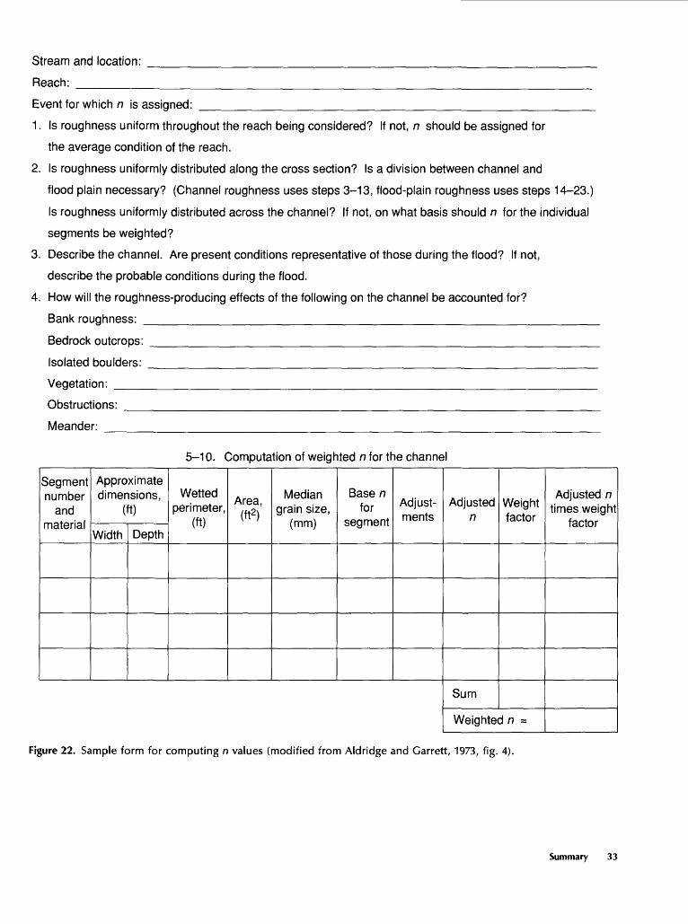
Stream and location: ___________________________________________

Reach: ____________________________________________________

Event for which n is assigned: ________________________________________

1. Is roughness uniform throughout the reach being considered? If not, n should be assigned for

the average condition of the reach.

2. Is roughness uniformly distributed along the cross section? Is a division between channel and

flood plain necessary? (Channel roughness uses steps 3-13, flood-plain roughness uses steps 14-23.)

Is roughness uniformly distributed across the channel? If not, on what basis should n for the individual

segments be weighted?

3. Describe the channel. Are present conditions representative of those during the flood? If not,

describe the probable conditions during the flood.

4. How will the roughness-producing effects of the following on the channel be accounted for?

Bank roughness: _____________________________________________

Bedrock outcrops: _____________________________________________

Isolated boulders: _____________________________________________

Vegetation: ________________________________________________

Obstructions:

Meander:

5-10. Computation of weighted n for the channel

Segment number

and material

Approximate dimensions,

(ft)

Width Depth

Wetted perimeter,

(ft)

Area,(ft2)

Median grain size,

(mm)

Base n for

segment

Adjust ments

Adjusted n

Sum

Weight factor

Weighted n =

Adjusted n times weight

factor

Figure 22. Sample form for computing n values (modified from Aldridge and Garrett, 1973, fig. 4).

Summary 33

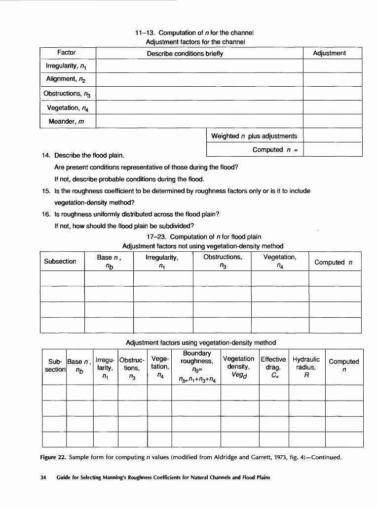
11-13. Computation of n for the channel Adjustment factors for the channel

Factor

Irregularity, n1

Alignment, n2

Obstructions, n3

Vegetation, n4

Meander, m

Describe conditions briefly

14. Describe the flood olain.

Weighted n plus adjustments

Computed n =

Adjustment

Are present conditions representative of those during the flood?

If not, describe probable conditions during the flood.

15. Is the roughness coefficient to be determined by roughness factors only or is it to include

vegetation-density method?

16. Is roughness uniformly distributed across the flood plain?

If not, how should the flood plain be subdivided?

17-23. Computation of n for flood plain Adjustment factors not using vegetation-density method

Subsection Base n , nb

Irregularity, "i

Obstructions,"3

Vegetation,A74 Computed n

Adjustment factors using vegetation-density method

Sub section

Base n , nb

Irregu larity,"i

Obstruc tions,

"3

Vege tation,

n4

Boundary roughness,

n0=

'V71 +n3+A74

Vegetation density,

Vegd

Effective drag,

c*

Hydraulic radius,

R

Computed n

Figure 22. Sample form for computing n values (modified from Aldridge and Garrett, 1973, fig. 4) Continued.


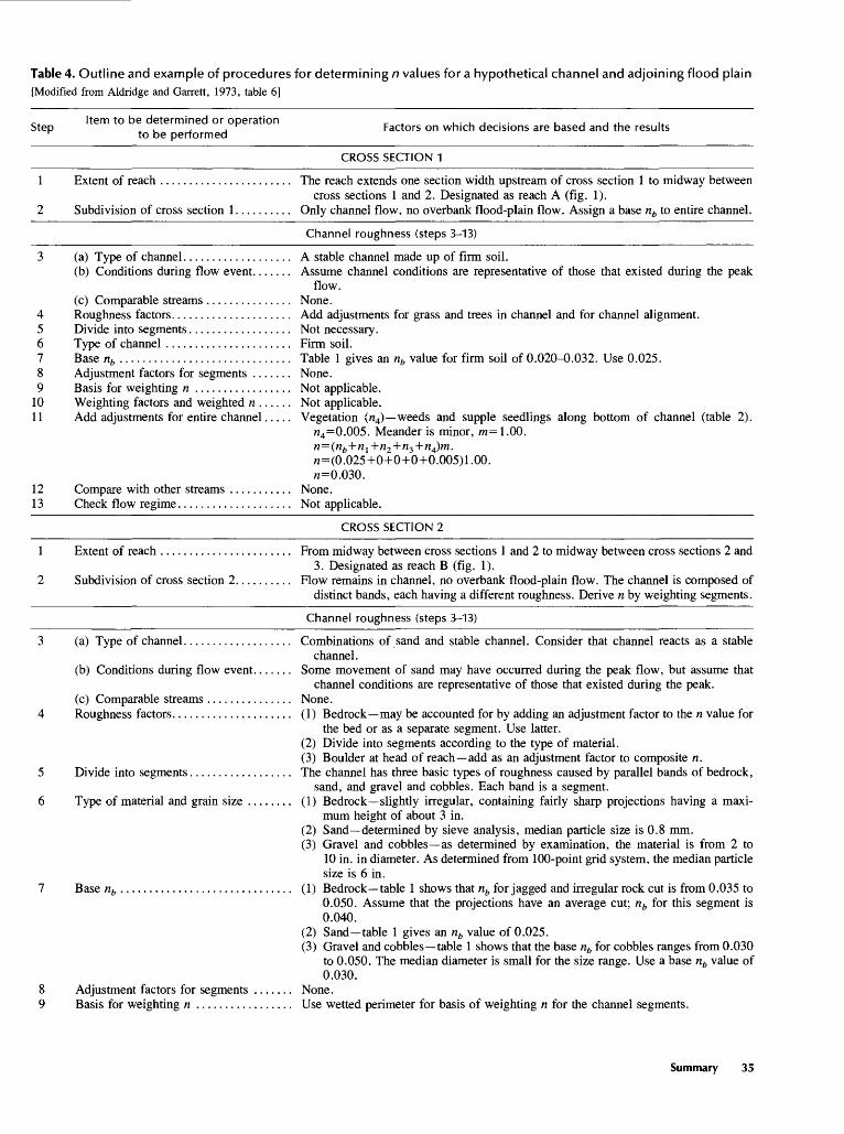
Table 4. Outline and example of procedures for determining n values for a hypothetical channel and adjoining flood plain[Modified from Aldridge and Garrett, 1973, table 6]

StepItem to be determined or operation

to be performedFactors on which decisions are based and the results

CROSS SECTION 1

1 Extent of reach ....................... The reach extends one section width upstream of cross section 1 to midway betweencross sections 1 and 2. Designated as reach A (fig. 1).

2 Subdivision of cross section 1.......... Only channel flow, no overbank flood-plain flow. Assign a base nb to entire channel.

Channel roughness (steps 3-13)

3 (a) Type of channel................... A stable channel made up of firm soil.(b) Conditions during flow event....... Assume channel conditions are representative of those that existed during the peak

flow.(c) Comparable streams ............... None.

4 Roughness factors..................... Add adjustments for grass and trees in channel and for channel alignment.5 Divide into segments.................. Not necessary.6 Type of channel ...................... Firm soil.7 Base nb .............................. Table 1 gives an nb value for firm soil of 0.020-0.032. Use 0.025.8 Adjustment factors for segments ....... None.9 Basis for weighting n ................. Not applicable.

10 Weighting factors and weighted n ...... Not applicable.11 Add adjustments for entire channel..... Vegetation («4) weeds and supple seedlings along bottom of channel (table 2).

«4 =0.005. Meander is minor, m=1.00. n (nb +n l +n2 +n3 + n4)m. n=(0.025+0+0+0+0.005)1.00. n=0.030.

12 Compare with other streams ........... None.13 Check flow regime.................... Not applicable.

CROSS SECTION 2

1 Extent of reach ....................... From midway between cross sections 1 and 2 to midway between cross sections 2 and3. Designated as reach B (fig. 1).

2 Subdivision of cross section 2.......... Flow remains in channel, no overbank flood-plain flow. The channel is composed ofdistinct bands, each having a different roughness. Derive n by weighting segments.

Channel roughness (steps 3-13)

3 (a) Type of channel................... Combinations of sand and stable channel. Consider that channel reacts as a stablechannel.

(b) Conditions during flow event....... Some movement of sand may have occurred during the peak flow, but assume thatchannel conditions are representative of those that existed during the peak.

(c) Comparable streams............... None.4 Roughness factors..................... (1) Bedrock may be accounted for by adding an adjustment factor to the n value for

the bed or as a separate segment. Use latter.(2) Divide into segments according to the type of material.(3) Boulder at head of reach add as an adjustment factor to composite n.

5 Divide into segments.................. The channel has three basic types of roughness caused by parallel bands of bedrock,sand, and gravel and cobbles. Each band is a segment.

6 Type of material and grain size ........ (1) Bedrock slightly irregular, containing fairly sharp projections having a maxi mum height of about 3 in.

(2) Sand determined by sieve analysis, median particle size is 0.8 mm.(3) Gravel and cobbles as determined by examination, the material is from 2 to

10 in. in diameter. As determined from 100-point grid system, the median particle size is 6 in.

7 Base nb .............................. (1) Bedrock table 1 shows that nb for jagged and irregular rock cut is from 0.035 to0.050. Assume that the projections have an average cut; nb for this segment is 0.040.

(2) Sand table 1 gives an nb value of 0.025.(3) Gravel and cobbles table 1 shows that the base nb for cobbles ranges from 0.030

to 0.050. The median diameter is small for the size range. Use a base nb value of 0.030.

8 Adjustment factors for segments ....... None.9 Basis for weighting n ................. Use wetted perimeter for basis of weighting n for the channel segments.

Summary 35

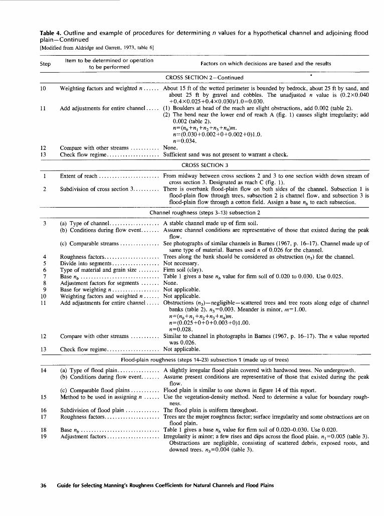
Table 4. Outline and example of procedures for determining n values for a hypothetical channel and adjoining flood plain Continued[Modified from Aldridge and Garrett, 1973, table 6]

_ Item to be determined or operation ... . . . , . . , , , . .Step , , , Factors on which decisions are based and the results

r to be performed

CROSS SECTION 2-Continued

10 Weighting factors and weighted n ...... About 15 ft of the wetted perimeter is bounded by bedrock, about 25 ft by sand, andabout 25 ft by gravel and cobbles. The unadjusted n value is (0.2x0.040 +0.4X0.025+0.4X0.030)71.0=0.030.

11 Add adjustments for entire channel..... (1) Boulders at head of the reach are slight obstructions, add 0.002 (table 2).(2) The bend near the lower end of reach A (fig. 1) causes slight irregularity; add

0.002 (table 2). n=(nb +n l +n2 +n3 +n4)m. n=(0.030+0.002+0+0.002+0)1.0. n=0.034.

12 Compare with other streams ........... None.13 Check flow regime.................... Sufficient sand was not present to warrant a check.

CROSS SECTION 3

1 Extent of reach ....................... From midway between cross sections 2 and 3 to one section width down stream ofcross section 3. Designated as reach C (fig. 1).

2 Subdivision of cross section 3.......... There is overbank flood-plain flow on both sides of the channel. Subsection 1 isflood-plain flow through trees, subsection 2 is channel flow, and subsection 3 is flood-plain flow through a cotton field. Assign a base nb to each subsection.

Channel roughness (steps 3-13) subsection 2

3 (a) Type of channel................... A stable channel made up of firm soil.(b) Conditions during flow event....... Assume channel conditions are representative of those that existed during the peak

flow.(c) Comparable streams ............... See photographs of similar channels in Barnes (1967, p. 16-17). Channel made up of

same type of material. Barnes used n of 0.026 for the channel.4 Roughness factors..................... Trees along the bank should be considered as obstruction («3) for the channel.5 Divide into segments.................. Not necessary.6 Type of material and grain size ........ Firm soil (clay).7 Base nb .............................. Table 1 gives a base nb value for firm soil of 0.020 to 0.030. Use 0.025.8 Adjustment factors for segments ....... None.9 Base for weighting n .................. Not applicable.

10 Weighting factors and weighted n ...... Not applicable.11 Add adjustments for entire channel..... Obstructions («3) negligible scattered trees and tree roots along edge of channel

banks (table 2). «3 =0.003. Meander is minor, m=1.00. n=(nb +n l +n2 +n3 +n4)m. n=(0.025+0+0+0.003+0)1.00. n=0.028.

12 Compare with other streams ........... Similar to channel in photographs in Barnes (1967, p. 16-17). The n value reportedwas 0.026.

13 Check flow regime.................... Not applicable.

Flood-plain roughness (steps 14-23) subsection 1 (made up of trees)

14 (a) Type of flood plain................ A slightly irregular flood plain covered with hardwood trees. No undergrowth.(b) Conditions during flow event....... Assume present conditions are representative of those that existed during the peak

flow.(c) Comparable flood plains ........... Rood plain is similar to one shown in figure 14 of this report.

15 Method to be used in assigning n ...... Use the vegetation-density method. Need to determine a value for boundary rough ness.

16 Subdivision of flood plain ............. The flood plain is uniform throughout.17 Roughness factors..................... Trees are the major roughness factor; surface irregularity and some obstructions are on

flood plain.18 Base nb .............................. Table 1 gives a base nb value for firm soil of 0.020-0.030. Use 0.020.19 Adjustment factors .................... Irregularity is minor; a few rises and dips across the flood plain. n l =0.005 (table 3).

Obstructions are negligible, consisting of scattered debris, exposed roots, and downed trees. «3 =0.004 (table 3).


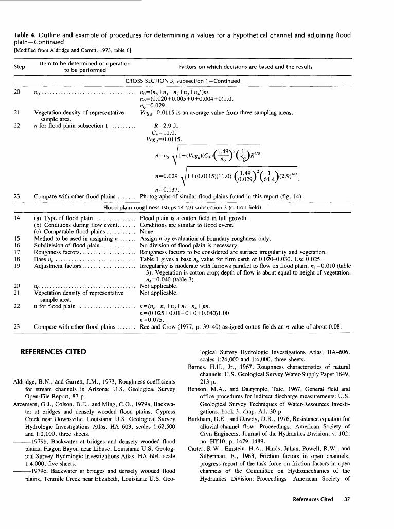
Table 4. Outline and example of procedures for determining n values for a hypothetical channel and adjoining floodplain Contin ued[Modified from Aldridge and Garrett, 1973, table 6]

StepItem to be determined or operation

to be performedFactors on which decisions are based and the results

CROSS SECTION 3, subsection 1 Continued

20

21

22

23

Vegetation density of representativesample area.

n for flood-plain subsection 1 .....

nQ =(nb +n l +n2 +n3 +n4 ')m.n0 =(0.020+0.005+0+0.004+0)1.0.n0 =0.029.Vegd=0.0ll5 is an average value from three sampling areas.

R=2.9 ft.

Vegd=Q.Qll5.

n=0.029

n=0.137. Compare with other flood plains ....... Photographs of similar flood plains found in this report (fig. 14).

Flood-plain roughness (steps 14-23) subsection 3 (cotton field)

14 (a) Type of flood plain................ Flood plain is a cotton field in full growth.(b) Conditions during flow event....... Conditions are similar to flood event.(c) Comparable flood plains ........... None.

15 Method to be used in assigning n ...... Assign n by evaluation of boundary roughness only.16 Subdivision of flood plain ............. No division of flood plain is necessary.17 Roughness factors..................... Roughness factors to be considered are surface irregularity and vegetation.18 Base nb .............................. Table 1 gives a base nb value for firm earth of 0.020-0.030. Use 0.025.19 Adjustment factors.................... Irregularity is moderate with furrows parallel to flow on flood plain, nÔ.010 (table

3). Vegetation is cotton crop; depth of flow is about equal to height of vegetation, n4 =0.040 (table 3).

20 «0 ................................... Not applicable.21 Vegetation density of representative Not applicable,

sample area.22 n for flood plain ..................... n=(nb +n l +n2 +n3 +n4 +)tn.

n=(0.025+0.01+0+0+0.040)1.00. n=0.075.

23 Compare with other flood plains ....... Ree and Crow (1977, p. 39^40) assigned cotton fields an n value of about 0.08.

REFERENCES CITED

Aldridge, B.N., and Garrett, J.M., 1973, Roughness coefficients for stream channels in Arizona: U.S. Geological Survey Open-File Report, 87 p.

Arcement, G.J., Colson, B.E., and Ming, C.O., 1979a, Backwa ter at bridges and densely wooded flood plains, Cypress Creek near Downsville, Louisiana: U.S. Geological Survey Hydrologic Investigations Atlas, HA-603, scales 1:62,500 and 1:2,000, three sheets.

1979b, Backwater at bridges and densely wooded flood plains, Flagon Bayou near Libuse, Louisiana: U.S. Geolog ical Survey Hydrologic Investigations Atlas, HA-604, scale 1:4,000, five sheets.

1979c, Backwater at bridges and densely wooded flood plains, Tenmile Creek near Elizabeth, Louisiana: U.S. Geo

logical Survey Hydrologic Investigations Atlas, HA-606, scales 1:24,000 and 1:4,000, three sheets.

Barnes, H.H., Jr., 1967, Roughness characteristics of natural channels: U.S. Geological Survey Water-Supply Paper 1849, 213 p.

Benson, M.A., and Dalrymple, Tate, 1967, General field and office procedures for indirect discharge measurements: U.S. Geological Survey Techniques of Water-Resources Investi gations, book 3, chap. Al, 30 p.

Burkham, D.E., and Dawdy, D.R., 1976, Resistance equation for alluvial-channel flow: Proceedings, American Society of Civil Engineers, Journal of the Hydraulics Division, v. 102, no. HY10, p. 1479-1489.

Carter, R.W., Einstein, H.A., Hinds, Julian, Powell, R.W., and Silberman, E., 1963, Friction factors in open channels, progress report of the task force on friction factors in open channels of the Committee on Hydromechanics of the Hydraulics Division: Proceedings, American Society of

References Cited 37

Civil Engineers, Journal of the Hydraulics Division, v. 89, no. HY2, pt. 1, p. 97-143.

Chow, V.T., 1959, Open-channel hydraulics: New York, McGraw-Hill Book Co., 680 p.

Colson, B.E., Arcement, G.J., and Ming, C.O., 1979, Backwater at bridges and densely wooded flood plains, Coldwater River near Red Banks, Mississippi: U.S. Geological Survey Hydrologic Investigations Atlas, HA-593, scales 1:24,000 and 1:8,000, three sheets.

Colson, B.E., Ming, C.O., and Arcement, G.J., 1979a, Backwa ter at bridges and densely wooded flood plains, Yockanoo- kany River near Thomastown, Mississippi: U.S. Geological Survey Hydrologic Investigations Atlas, HA-599, scales 1:62,500 and 1:8,000, nine sheets.

1979b, Backwater at bridges and densely wooded flood plains, Thompson Creek near Clara, Mississippi: U.S. Geo logical Survey Hydrologic Investigations Atlas, HA-597, scales 1:24,000 and 1:8,000, three sheets.

Cowan, W.L., 1956, Estimating hydraulic roughness coefficients: Agricultural Engineering, v. 37, no. 7, p. 473-475.

Henderson, P.M., 1966, Open-channel flow: New York, Mac- Millan Publishing Co., Inc., 522 p.

Limerinos, J.T., 1970, Determination of the Manning coefficient from measured bed roughness in natural channels: U.S. Geological Survey Water-Supply Paper 1898-B, 47 p.

Ming, C.O., Colson, B.E., and Arcement, G.J., 1979, Backwater at bridges and densely wooded flood plains, Pea Creek near

Louisville, Alabama: U.S. Geological Survey Hydrologic Investigations Atlas, HA-608, scales 1:24,000 and 1:2,000, three sheets.

Petryk, Sylvester, and Bosmajian, George, III, 1975, Analysis of flow through vegetation: Proceedings, American Society of Civil Engineers, Journal of the Hydraulics Division, v. 101, no. HY7, p. 871-884.

Ree, W.O., 1954, Handbook of channel design for soil and water conservation: Soil Conservation Service, U.S. Department of Agriculture, SCS-TP-61, 40 p.

Ree, W.O., and Crow, F.R., 1977, Friction factors for vegetated waterways of small slope: Agricultural Research Service, U.S. Department of Agriculture, ARS-S-151, 56 p.

Schneider, V.R., Board, J.W., Colson, B.E., Lee, F.N., and Druffel, Leroy, 1977, Computation of backwater and dis charge at width constrictions of heavily vegetated flood plains: U.S. Geological Survey Water-Resources Investiga tions 76-129, 64 p.

Simons, D.B., and Richardson, E.V., 1966, Resistance to flow in alluvial channels: U.S. Geological Survey Professional Paper 422-J, 61 p.

Simons, D.B., Li, R.M., and Associates, 1982, Resistance to flow in alluvial channels, chap. 6, in Engineering analysis of fluvial systems: Fort Collins, Colorado, Simons, Li, and Associates, p. 6.11-6.17.

Streeter, V.L., 1971, Fluid mechanics: New York, McGraw-Hill Book Co., 5th ed. 705 p.


Documents

Guide for Selecting Manning's Roughness Coefficients for