Embed Size (px)
Citation preview

U.S. Department of the Interior Bureau of Reclamation Technical Service Center Denver, Colorado August 2013
Guidelines for Collecting Data to Support Statistical Analysis of Water Quality for Wetland Planning

Mission Statements The U.S. Department of the Interior protects America’s natural resources and heritage, honors our cultures and tribal communities, and supplies the energy to power our future. The mission of the Bureau of Reclamation is to manage, develop, and protect water and related resources in an environmentally and economically sound manner in the interest of the American public.
U.S. Department of the Interior Bureau of Reclamation Technical Service Center Denver, Colorado August 2013
Guidelines for Collecting Data to Support Statistical Analysis of Water Quality for Wetland Planning

iii
Contents
Page
Executive Summary .............................................................................................. 1 Six Data Collection Recommendations for Wetland Water Quality
Statistical Analysis ................................................................................ 2
What is Covered in These Guidelines? ............................................................... 5
Application............................................................................................................. 8
Defining the System .............................................................................................. 8 Wetland Delineation ......................................................................................... 9 Constructed Wetlands Design Considerations ................................................ 10 Major Wetland Functions ............................................................................... 12 Staged or Pretreatment Wetlands .................................................................... 12 Processes Affecting Wetlands ......................................................................... 12
Develop the Sample Analysis Plan..................................................................... 14 Short- and Long-term Operational Factors and Operations Data ................... 15 Water Quality .................................................................................................. 17 Wetland Vegetation ........................................................................................ 19 Aquatic Biota .................................................................................................. 22 Birds (Swimming, Diving, and Nesting) ........................................................ 22 Habitat and Regulations .................................................................................. 23 Fish and Reptiles ............................................................................................. 24 Aerial and Topographic Data .......................................................................... 24 Meteorological Data........................................................................................ 25
Identify Upstream Boundary Conditions ......................................................... 26
Hydraulics Analysis ............................................................................................ 28 Dye Studies for Wetland Hydraulics .............................................................. 28 HLR and HRT Analysis .................................................................................. 31 Flows and Water Mass Balance Data ............................................................. 32 Wetland Water Mass Balance Data Sources ................................................... 32 Flow Monitoring and Data Compilation ......................................................... 32 Water Budget Data Gaps and Empirical Model Considerations .................... 32 Hydrodynamics and Short-circuiting .............................................................. 33 Cross-sectional Channel Geometry Survey Methods ..................................... 33 Digital Mapping Data Format and Processing ................................................ 34 Grid Considerations ........................................................................................ 34
Selecting Sampling Locations ............................................................................ 35
Statistical Data Analyses .................................................................................... 38 Different Types of Statistical Analysis ........................................................... 39
Guidelines for Collecting Data to Support Statistical Analysis of Water Quality for Wetland Planning
iv
Data Analysis Requirements ........................................................................... 42 Data Gaps and Model Considerations............................................................. 45 Role of Statistical Analysis in Wetland Planning and Design ........................ 45 Statistical Model Testing ................................................................................ 46 Other Statistical Model Data Collection Considerations ................................ 46
Data Collection Priorities and Practical Considerations ................................ 47 Prioritizing Critical and Secondary Data Sets ................................................ 47 Existing Data Sources and Data Compilation ................................................. 47 Monitoring Plans and Cost Factors ................................................................. 47 Data Review, Analysis, and Processing Concerns.......................................... 47
Conclusions .......................................................................................................... 48
References ............................................................................................................ 49 Tables Page Table 1.—Field data used for water quality analysis ........................................... 17 Table 2.—Site water quality monitoring parameter groups ................................. 27 Table 3.—Field data used for wetland delineation, flow mass balance, and
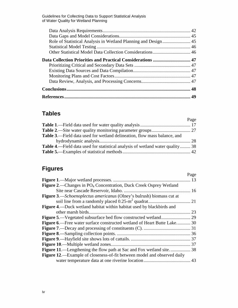
hydrodynamic analysis.............................................................................. 28 Table 4.—Field data used for statistical analysis of wetland water quality ......... 38 Table 5.—Examples of statistical methods .......................................................... 42 Figures Page Figure 1.—Major wetland processes. .................................................................. 13 Figure 2.—Changes in PO4 Concentration, Duck Creek Osprey Wetland
Site near Cascade Reservoir, Idaho. ......................................................... 16 Figure 3.—Schoenoplectus americanus (Olney’s bulrush) biomass cut at
soil line from a randomly placed 0.25-m2 quadrat .................................... 21 Figure 4.—Duck wetland habitat within habitat used by blackbirds and
other marsh birds....................................................................................... 23 Figure 5.—Vegetated subsurface bed flow constructed wetland ......................... 29 Figure 6.—Free water surface constructed wetland of Heart Butte Lake. ........... 30 Figure 7.—Decay and processing of constituents (C). ........................................ 31 Figure 8.—Sampling collection points. ............................................................... 36 Figure 9.—Hayfield site shows lots of cattails. ................................................... 37 Figure 10.—Multiple wetland zones. ................................................................... 37 Figure 11.—Lengthening the flow path at Sac and Fox wetland site. ................. 38 Figure 12.—Example of closeness-of-fit between model and observed daily
water temperature data at one riverine location ........................................ 43
Guidelines for Collecting Data to Support Statistical Analysis of Water Quality for Wetland Planning
1
Executive Summary The Reclamation manuals and standards program funded this document. Wetlands will play a vital role in ecosystem restoration which is a primary goal of the Bureau of Reclamation as stated below:
Ecosystem Restoration — In order to meet Reclamation's mission goals of securing America's energy resources and managing water in a sustainable manner for the 21st century, a part of its programs must focus on the protection and restoration of the aquatic and riparian environments affected by its operations. Ecosystem restoration involves a large number of activities, including Reclamation's Endangered Species Act recovery programs, which are required in order to continue project operations and directly address the environmental aspects of the Reclamation mission (Testimony for FY12 budget request by Michael L. Connor, Bureau of Reclamation (Reclamation) Commissioner, March 2, 2011 before Natural Resources Committee, Subcommittee on Water and Power, U.S. House of Representatives).
The primary focus of these guidelines is the planning, data collection, and design aspects of multi-purpose wetlands to meet Reclamation ecosystem restoration goals, which include improved water quality. Both hydraulic analysis and statistical analysis of wetlands are necessary for proper design. Monitoring of water quality, wetland health, and wildlife habitat is equally necessary for proper evaluation of the systems and subsequent development of future designs.
Statistical analysis of water quality parameters is a useful tool for exploring ecosystem restoration in wetland environments. There are several types of statistical analysis techniques and each requires a unique set of inputs that are specific to a particular situation. Much of wetland statistical analysis success can be tied to the selection of the data parameters, frequency, and tools to be used. The layout of the wetland Sampling Analysis Plan (SAP), which describes the type of data, as well as when, where, and how often data are collected is a critical planning stage.
These guidelines provide some important data collection tips and references for analyzing natural and constructed wetlands. The following recommendations provide direction for wetland analysis and ecosystem restoration.
Guidelines for Collecting Data to Support Statistical Analysis of Water Quality for Wetland Planning
2
Six Data Collection Recommendations for Wetland Water Quality Statistical Analysis
There are six important input data recommendations for wetland water quality analysis and ecosystem restoration. These are discussed below.
Differentiate Between Natural and Constructed Wetlands Wetlands are constructed for water quality improvement and provide buffering capacity in regards to temperature, DO, pH, and other constituents thereby damping the effects of spikes and diel variations (Kadlec and Knight, 1996 and Bureau of Reclamation, 2008). The type of wetland design dictates the model or statistical analysis technique chosen to assess wetland performance at improving water quality goals. The first step is to identify or define the system as a natural wetland or a design/constructed wetland.
Identify Upstream Boundary Conditions Upstream boundary conditions are important to wetland analysis; therefore, it is important to select appropriate upstream wetland inflow locations where data are to be collected such as at a bridge, weir, or gage. Collect reconnaissance wetland inflow water quality data before development of the sampling analysis plan (SAP) sampling locations, frequency of sampling, and the desired list of water quality parameters. Water quality data should include critical chemical specific parameters targeted for water quality improvement as well as bulk physical and hydraulic information.
Selecting Sampling Locations The sampling protocol for the selected analysis (such as the wetland locations, bridge and weir locations, and segments) should be identified early. Data collection layout should be carefully considered before data collection; it is how wetlands are constructed that makes them effective at water treatment. A common mistake is to place a gage or collect samples in a recirculation eddy, backwater area, or in a location where solar radiation directly shines on a thermistor. Samples that are representative of a completely-mixed plug-flow condition should be collected. If stratification occurs in wetland pools, vertical water quality profiles over depth may be necessary. Hyporheic groundwater inflow may produce lateral gradients across the wetland and thermal refugia; data may need to be collected laterally on each side of the main flow path through the wetland.
Executive Summary
3
Develop a Wetland Sample Analysis Plan (SAP) Water quality parameters will need to be chosen and water quality indicators may need to be developed for the wetland SAP. In addition to water quality parameters, some of the most important variables for wetland analysis are hydraulic loading rate (HLR), hydraulic retention time (HRT), and water depths. Finally, the general wetland health will need to be monitored through the collection of data and observations related to vegetation, wildlife, habitat, and meteorological conditions. Therefore, water quality, hydraulic parameters, and wetland indicators should be defined early and collected over several seasons and several hydrologic inflow and outflow conditions (wet versus dry conditions and years) to properly evaluate the system.
Hydraulics Analysis A primary objective of wetland hydraulic analysis is to adequately express the water residence times in the wetland which affect decay and transformations of inflow organics and nutrients. Wetland performance is a function of hydraulic retention time (HRT), which is related to inflow and outflow dynamics, water depth, and short-circuiting. Dye travel time studies are often necessary to identify short-circuiting via the least restrictive path. Hydraulic load rate (HLR) is also an important concept when considering wetland design and whether the wetland is sustainable over time. Vegetative growth, treatment goals, and wildlife issues are necessary to identify when determining the HLR. Surface water and groundwater hydraulic information must be collected to determine an adequate water mass balance that relates to wetland flushing in relation to changes in wetland water surface elevation. Sufficient data for a minimum of a monthly flow mass balance needs to be collected.
Statistical Data Analysis Sufficient water quality data needs to be collected to provide a statistically significant foundation for analyzing the water quality data. Carefully planned input data sets prevent problems during statistical analysis. As many as thirty data points for each parameter might need to be collected to provide an adequate sample population. Design the data collection around planned statistical analysis; collect enough data to show statistical significance. Be aware and provide proper considerations for temporal variations in water quality. For instance, day and night temperature and dissolved oxygen swings and changes in flow and water quality conditions over time affect wetland water quality. These factors and other factors should be considered when collecting and developing data sets for statistical analysis.


Guidelines for Collecting Data to Support Statistical Analysis of Water Quality for Wetland Planning
5
What is Covered in These Guidelines? These guidelines focus on traditional wetland systems indicative of relatively dry western areas of the United States. Due to large sediment load which can quickly fill a wetland, pretreatment sedimentation wetlands and staged wetlands are mentioned. The following guidelines were written with an emphasis on planning for wetland water quality data collection, wetland examples, statistical analysis, and loading models. Some of those statistical or modeling approaches are described in Appendix A. Common ecological and wetland modeling techniques are also reviewed only briefly. Data collected for reservoir models differ and are covered in a separate document (Bureau of Reclamation, 2009). Data collected for riverine models also differ and are covered in a separate document (Bureau of Reclamation, 2010). Riverine models could provide the upstream boundary inflow conditions for wetland studies. The many details of wetland analysis cannot be covered in a single document. Many and various specific types of wetland manuals exist. Due to extensive published literature on the various topics associated with wetlands, these guidelines will simply reference rather than repeat that information.
For example, the United States Environmental Protection Agency (EPA, September, 2000) prepared a manual entitled “Constructed Wetlands Treatment of Municipal Wastewater” for a non-technical audience that references several previous manuals. The EPA (short for USEPA) manual discusses common misconceptions of constructed wetlands, addresses frequently asked questions, discusses treatment mechanisms occurring in a constructed wetland, describes limitations, and provides an introduction to constructed wetland design, construction, startup, and operational issues.
Reclamation feasibility design guidelines for wetlands (Bureau of Reclamation, 2008) also exist and cover regulatory considerations, guiding principles, and feasibility report requirements specific to wetland projects. The following guidelines try to avoid duplication of material covered or referenced in existing manuals or guidelines. Excellent guidance and training courses exist for constructed wetlands. Technical and regulatory guidance for constructed treatment wetlands is taught by the Interstate Technology Regulatory Council (ITRC) and is supported by many government departments including EPA.
For additional details, including sizing details, see the following reference: Environmental Protection Agency, September 1988, “Design Manual: Constructed Wetlands and Aquatic Plant Systems for Municipal Wastewater Treatment,” EPA/625/1-88/022, Office of Research and Development, Cincinnati, OH. http://water.epa.gov/type/wetlands/upload/design.pdf
Guidelines for Collecting Data to Support Statistical Analysis of Water Quality for Wetland Planning
6
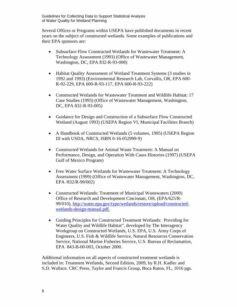
Several Offices or Programs within USEPA have published documents in recent years on the subject of constructed wetlands. Some examples of publications and their EPA sponsors are:
• Subsurface Flow Constructed Wetlands for Wastewater Treatment: A Technology Assessment (1993) (Office of Wastewater Management, Washington, DC, EPA 832-R-93-008)
• Habitat Quality Assessment of Wetland Treatment Systems (3 studies in 1992 and 1993) (Environmental Research Lab, Corvallis, OR, EPA 600-R-92-229, EPA 600-R-93-117, EPA 600-R-93-222)
• Constructed Wetlands for Wastewater Treatment and Wildlife Habitat: 17 Case Studies (1993) (Office of Wastewater Management, Washington, DC, EPA 832-R-93-005)
• Guidance for Design and Construction of a Subsurface Flow Constructed Wetland (August 1993) (USEPA Region VI, Municipal Facilities Branch)
• A Handbook of Constructed Wetlands (5 volumes, 1995) (USEPA Region III with USDA, NRCS, ISBN 0-16-052999-9)
• Constructed Wetlands for Animal Waste Treatment: A Manual on Performance, Design, and Operation With Cases Histories (1997) (USEPA Gulf of Mexico Program)
• Free Water Surface Wetlands for Wastewater Treatment: A Technology Assessment (1999) (Office of Wastewater Management, Washington, DC, EPA /832/R-99/002)
• Constructed Wetlands: Treatment of Municipal Wastewaters (2000) Office of Research and Development Cincinnati, OH, (EPA/625/R-99/010), http://water.epa.gov/type/wetlands/restore/upload/constructed-wetlands-design-manual.pdf.
• Guiding Principles for Constructed Treatment Wetlands: Providing for Water Quality and Wildlife Habitat”, developed by The Interagency Workgroup on Constructed Wetlands, U.S. EPA, U.S. Army Corps of Engineers, U.S. Fish & Wildlife Service, Natural Resources Conservation Service, National Marine Fisheries Service, U.S. Bureau of Reclamation, EPA 843-B-00-003, October 2000.
Additional information on all aspects of constructed treatment wetlands is included in: Treatment Wetlands, Second Edition, 2009, by R.H. Kadlec and S.D. Wallace. CRC Press, Taylor and Francis Group, Boca Raton, FL, 1016 pgs.
What is Covered in These Guidelines?
7
Purpose and Scope of Guidelines These guidelines provide insight to help prioritize types of data and how the data need to be collected. The guidelines start by briefly describing the baseline or upstream boundary conditions necessary for evaluating the performance of the wetland system. Next the guidelines focus on the data collection that would need to be captured in a SAP tailored for a specific project. A SAP answers questions such as what, where, when, how, with what equipment, to what standards and quality assurance/quality control (QA/QC), and who is responsible for collecting the flow, sediment, and water quality data.
Sampling protocols, field and laboratory QA/QC, analytical methods, data processing, and data storage issues are addressed in “Quality Assurance Guidelines for Environmental Measurement” (Bureau of Reclamation, 2002 revised August 2003). The “Quality Assurance Guidelines for Environmental Measurements” provide templates in many areas of the planning and data collection process. The “Technical Guidelines for Water Quality Investigation” (Bureau of Reclamation, September 2003) cover additional technical details, approaches, and general information for planning water quality investigations.
Next the guidelines focus on describing the need for hydraulic analysis and the determination of HLR and HRT. A primary objective of wetland hydraulic analysis is to adequately express the water residence times in the wetland which affect decay and processing of inflowing organics and nutrients. Tracer dye tests are described for determining wetland hydraulics to describe water quality constituent attenuation as well as to identify stagnant, non-effective areas.
The guidelines also address data collection to address both parametric and non-parametric statistical methods. These guidelines address critical data necessary to support empirical modeling techniques. However, the data could be used to support other modeling approaches. Data must be collected in advance to accurately represent the actual conditions of interest. For example, to accurately predict how structural or operational modifications would influence wetland conditions during low flows, water quality analysis should incorporate data collected during low-pool low-flushing conditions.
Unfortunately, data collection efforts in support of wetland statistical analysis are often not completed and are many times abandoned due to economic constraints. Therefore, data collection priorities and practical considerations are covered in these guidelines to maximize data collection activities in support of wetland statistical analysis. A few statistical data sets, in combination with sensitivity analysis, provide insight into the water quality conditions of wetlands and how to alter or design wetlands for improved water quality.
Guidelines for Collecting Data to Support Statistical Analysis of Water Quality for Wetland Planning
8
Application The primary application of the following guidelines is for data collection supporting wetlands in arid environments of the western United States. The three categories of wetland systems in such environments are natural wetlands, surface flow (SF) systems with a weir outlet, and subsurface flow (SSF) systems with an adjustable standpipe.
Often Reclamation’s wetland restoration activity is aimed at replacing wetland functions and values lost as a result of building irrigation water delivery systems. Wetlands may be used to minimize adverse impacts of irrigation return water or wastewater discharges of various kinds into natural water bodies (EPA, Edited by Olsen, 1993, page 204.) Appropriate planning for environmental data collection and processing is critical to overall success in developing accurate predictive empirical modeling capability.
EPA (Olsen, 1993) provided some preliminary principles of natural wetland design. The wetland should be designed for minimal maintenance, to utilize natural energies, in anticipation of floods and droughts, with multiple objectives, as a buffering ecosystem, for specific functions, and not over-engineered with rectangular basins, rigid structures, and channels. If possible, wetlands should be designed to enhance existing natural systems.
Reference:
Environmental Protection Agency, 1993, “Created and Natural Wetlands for Controlling Nonpoint Source Pollution,” Edited by Richard K. Olsen, Office of Research and Development and Office of Wetlands, Oceans, and Watersheds, C. K. Smoley, CRC Press, Inc., Boca Raton, Florida.
Defining the System Treatment wetlands are constructed for water quality improvement and provide buffering capacity in regards to temperature, DO, pH, and other constituents thereby damping the effects of spikes and diel variations (Kadlec and Knight, 1996 and Bureau of Reclamation, 2008). Due to sun and wind energies, wetlands can be inexpensive to operate and maintain. The type of wetland dictates the
model or statistical analysis technique chosen to assess wetland performance at improving water quality goals. The first step is to identify or define the system as a natural wetland or a non-natural design/constructed wetland.
There are three types of naturally flooded wetland treatment systems: facultative ponds designed to maintain a naturally aerated surface layer over a deeper anaerobic layer, floating aquatic plant-based systems, and more traditional surface
Defining the System
9
flow emergent vegetation wetland systems. Natural wetlands might not require a full-blown design process. Dikes and outlet weir controls might be constructed by using local farm equipment at minimal cost. Conversely, design of a polishing pond for wastewater treatment plant discharges to potentially remove specific contaminants may require extensive planning, design, and post-monitoring. Wetlands should be designed based on the water quality going into the most upstream wetland, i.e., if the water is high in NH4-N, it should be designed with a high proportion of open water to vegetated area, compared to water high in NO3-N. Much has been written on designing constructed wetlands and new designs for more specific constituent removal are being investigated for their effectiveness and sustainability (i.e., EPA, 1998; EPA 2000; Sartoris et al., 2000a,b; Thullen et al., 2005; Kadlec and Wallace, 2009; Daniels, pers. comm. 2013).
Secondary treatment is the minimal level of municipal and industrial treatment that is required in the United States before discharge to most receiving waters such as a wetland. Secondary treatment requires a treatment level that will produce 5-day BOD and TSS concentrations of less than 30 mg/L and, in addition, a minimum percent concentration reduction of 85 percent (Kadlec and Knight, 1996). The generation of sedimentary material (algal biomass, litter fall, and so forth) is an important process in nutrient rich wetlands that contributes to the irreducible background portion of TSS. Therefore, wetlands should be overdesigned in terms of TSS reduction; however this is rarely carried out. TSS has an organic component that decays. Wetlands experiencing large flooding events could fill with sediment that does not decay and could be rendered useless or of diminished functionality.
Well-calibrated numeric wetland dynamic flow and water quality statistical tools (empirical models) are useful for predicting and evaluating the implications of structural or operational alternatives before undertaking expensive modifications. Statistical results depend on the underlying input data to produce an empirical model that accurately represents the varying water quality from low-pool to high-inflow (flushing) conditions. Wetland water quality data for statistical analysis requires planning and data collection several months or years in advance. A developing wetland with increasing vegetation also results in increased friction of flowing water. These dynamic and evolutionary changes can occur over many years. Therefore, bottom slope should not be considered as the design driving force for water movement. The reason is that designs based on bed slope are excessively sensitive to changing conditions of flow and hydraulic conductivity; dryout or flooding are virtually certain to occur with such designs, (Kadlec and Knight, 1996, page 228), thereby endangering wetland vegetation establishment.
Wetland Delineation For natural wetlands, the initial step in identifying a wetland is to check the National Wetlands Inventory (NWI) or Local Wetlands Inventory maps and to verify the presence of hydric (water logged) soils and hydrophytes, which are
Guidelines for Collecting Data to Support Statistical Analysis of Water Quality for Wetland Planning
10
plants that have special adaptations for life in permanently or seasonally saturated soils. Such areas are rarely tilled or tilled late into the season, would tend to fail a septic system test, are poorly drained, and produce rusty-red, mottled or gray soggy soils. Undrained hydric soils are saturated enough to develop anaerobic conditions that favor the growth of vegetation that have adapted to flooded or saturated environments.
Identifying and delineating wetlands by vegetation, soil, and hydrology as discussed by Hammer (1992) is necessary for regulatory jurisdiction under Section 404 of the Clean Water Act (33 U.S.C. 1344). For wetland delineation use the regional supplements to the following Environmental Laboratory reference:
United States Army Corp of Engineers (USACE), Environmental Laboratory, January 1987, “Corps of Engineers Wetlands Delineation Manual,” Final Technical Report Y-87-1 USACE Waterways Experiment Station, Vicksburg, MS http://el.erdc.usace.army.mil/wetlands/pdfs/wlman87.pdf
A list of the regional supplements can be found at the following web site.
http://www.usace.army.mil/cecw/pages/reg_supp.aspx
For Reclamation, “The Interim Regional Supplement to the Corps of Engineers Wetland Delineation Manual: Western Mountains, Valleys, and Coast Regions,” by the USACE is a useful document for western states and is referenced below:
U.S. Army Corp of Engineers, April 2008, “The Interim Regional Supplement to the Corps of Engineers Wetland Delineation Manual: Western Mountains, Valleys, and Coast Regions,” Final Report No. ERDC/EL TR-08-13, Environmental Laboratory, USACE Environmental Research and Development Center, Vicksburg, MS. http://www.usace.army.mil/CECW/Documents/cecwo/reg/west_mt_finalsupp.pdf
Constructed Wetlands Design Considerations
Wetlands are constructed for water quality improvement by building systems to maximize desired functions that occur naturally. Aquatic vegetation, whether emergent, submergent or floating, serve as treatment components. Wetland soils trap a variety of chemical constituents via physical (filtering) and chemical (sorption) mechanisms. Wetlands are ideal for chemical transformations (oxidation and reduction) because of the range of oxidation states (both positive and negative redox potential) and metabolism of microbes. Wetland pollution reduction processes may often be modeled with first-order, area-based equations of the form.
𝐽𝐽 = 𝑘𝑘 (𝐶𝐶 − 𝐶𝐶∗)
Defining the System
11
Where:
C = pollutant concentration, g/m3 C* = background pollutant concentration, g/m3 J = reduction rate, g/m2/yr k = rate constant, m/yr
Kadlec and Knight (1996) provide extensive coverage of k-C* first-order area-based models.
Wetlands provide buffering capacity in regards to temperature, DO, pH, and other constituents thereby damping the effects of spikes and diel variations (Kadlec and Knight, 1996 and Bureau of Reclamation, 2008). However, wetland vegetation does not filter out pollutants in conventional straining terms due to open water and voids between stems. Wetland vegetation enhances settling, reduces the effects of wind, and prevents resuspension of contaminants. Sequestration of pollutants and wetland processing of nutrients varies by wetland according to its HRT, HLR, design and location of aerobic and anaerobic zones and physical and meteorological conditions.
Wetland soils trap a variety of chemical constituents via physical (filtering) and chemical (sorption) mechanisms. Microbes (including nitrifying and denitrifying bacteria and algae) throughout wetlands perform many of the chemical transformations (oxidation and reduction) because of the range of oxidation states (both positive and negative redox potential) that occur through their metabolism. Additionally, open water zones are important components in wetlands because photolysis and volatilization occur at the air/water interface.
Many individuals and organizations contributed to the writing of the following topics. Moshiri (1993) touches on the subject of designing constructed wetlands in the following reference: Moshiri, Gerald A., 1993, “Constructed Wetlands for Water Quality Improvement,” CRC Press, Inc., Lewis Publishers, Boca Raton, ISBN 0-87371-550-0, Library of Congress Card Number 92-46759.
However, Kadlec and Knight (1996) greatly expanded upon the concepts and defined the state-of-the-art in the following reference: Kadlec, Robert H. and Knight, Robert L., (1996), “Treatment Wetlands,” CRC Press, Inc., Lewis Publishers, Boca Raton, ISBN 0-87371-930-1, Library of Congress Card Number 95-9492. Subsequently the reference was updated by Kadlec, Robert H., and Wallace, Scott D., (2009) in Treatment Wetlands: Second Edition,” CRC Press, Inc., Lewis Publishers, Taylor and Francis Group, Boca Raton, ISBN 978-1-56670-526-4. Wetland vegetation is further discussed by Cronk and Fennessy (2001) in Cronk, Julie K. and Fennessy, M. Siobhan, 2001, “Wetland Plants, Biology and Ecology,” CRC Press, Inc., Lewis Publishers, Boca Raton, ISBN 1-56670-372-7, Library of Congress Card Number 2001020390.
Guidelines for Collecting Data to Support Statistical Analysis of Water Quality for Wetland Planning
12
Major Wetland Functions
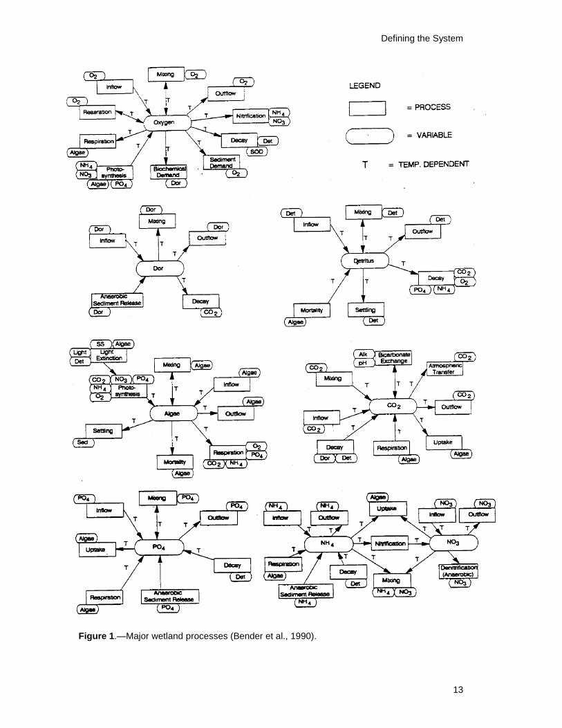
Wetlands are complex and the many components work together to serve many functions including shoreline stabilization, erosion control, flood control, sediment trapping, nutrient and contaminate reduction (including total coliforms), wildlife and fishery habitat, and recreation (http://old.geog.psu.edu/wetlands/ manual/chapter1.html and http://old.geog.psu.edu/wetlands/manual/toc.html#top). Figure 1 illustrates the many functions and how they interact.
Other literature sources including those from the U.S. Army Corp of Engineers (Smith et al., October 1995, Table 2) describe wetland functions and value.
Staged or Pretreatment Wetlands
Pretreatment wetlands can be used to capture sediment load before the water enters the wetland designed for the particular objective. A pretreatment wetland can also be designed to help minimize eventual short-circuiting or overland flooding and resuspension concerns in the design wetland.
Typically sediment resuspension in wetlands is inhibited by the litter mat and vegetation communities. Such a low-velocity laminar condition requires designing within the laminar range for both particle settling and resuspension (shear stress that tears loose particles) (Kadlec and Knight, 1996, page 322) taking care to factor in the prevailing winds of the area.
Processes Affecting Wetlands
Processes affecting wetlands could include the following:
• Subsurface inter-flow: Water supplied to the pond by a watershed field(s) deep seepage.
• Bank runoff: Runoff from exposed pond banks above the current inundation level.
• Input pump: A system delivering water from elsewhere such as an off-stream pump or an animal housing flush system.
• Precipitation: That falling directly on the currently inundated pond surface.
• Evaporation: Loss from the water surface estimated as the potential daily evaporation.
• Infiltration: An amount infiltrating into the dry pond bottom as it is initially inundated.
• Seepage: A constant seepage beneath the inundated area.
Defining the System
13
Figure 1.—Major wetland processes (Bender et al., 1990).
Guidelines for Collecting Data to Support Statistical Analysis of Water Quality for Wetland Planning
14
• Pipe outlet: Flow of a pipe outlet system having a defined stage-discharge relationship.
• Spillway overflow: An uncontrolled daily flow from the uppermost spillway or outlet.
• Supply pump: An amount pumped from the pond for designated rates and periods with a specified inlet pond depth, e.g. to supply an animal watering water tank.
• Discharge pump: An amount pumped from the pond for designated rates and periods with a specified inlet pond depth, e.g. to remove lagoon water to a disposal field.
• Irrigation: An amount supplied to one or more fields for an irrigation depth for each irrigated field.
Develop the Sample Analysis Plan Water quality parameters will need to be chosen and water quality indicators may need to be developed for the wetland sampling analysis plan (SAP). In addition to water quality parameters, some of the most important variables for wetland analysis are hydraulic loading rate (HLR) and hydraulic retention time (HRT). Finally, the general wetland health will need to be monitored through the collection of data and observations related to vegetation, wildlife, habitat, and meteorological conditions. Many questions need to be answered before going in the field to collect wetland data including:
• Where are the representative sample locations into or within the wetland?
• Instrument calibrations or sample bottle holding times?
• Synoptic sampling during a few days or long term sampling over months?
• Duplicates, blanks, rinsate blanks, replicates, splits, spikes, lab round-robins, and references?
• Half meter, one meter, five feet, pool bottom, surface, grabs, integrated composites or continuous sampling?
• Monthly, bi-weekly, weekly, daily, hourly, continuous, or telemetered data?
• U.S. Geological Survey (USGS), Environmental Protection Agency (EPA), or Standard Method (American Public Health Association (APHA), American Water Works Association (AWWA), and Water Environment Federation (WEF), 2005) protocols and procedures?
• Meta-data, recording procedures, and chain-of-custody?

Develop the Sample Analysis Plan
15
Other considerations include:
• Sampling to accommodate laboratory analysis procedures
• Job Hazard Analysis (JHA)
• Data processing
• Archival of data for future projects
• Empirical statistical model predictions or evaluations
• “Honoring” the data with metadata for future uses and summarizing data before writing a final data summary report
• Project oversight and peer review
• Planning for future automated data collection and telemetry to a nearby data center
• Selective data archival for future trend analysis Collecting environmental data is not a simple process and requires adequate planning. One drawback of a wetland study is that natural systems often respond slowly to operational changes and are greatly affected by uncontrolled natural events. A large flooding event can quickly fill a wetland with sediment thereby reducing the effectiveness of the original design. In such cases, sediment-trapping vegetative buffer strips or other erosion control measures might be required. In cases with large sediment runoff, off-channel wetlands might be used. Therefore, water quality, hydraulic parameters, and wetland indicators should be defined early and collected over several seasons and several hydrologic inflow and outflow conditions (wet versus dry conditions and years) to properly evaluate the system.
Short- and Long-term Operational Factors and Operations Data
Operations data are not directly required for statistical analysis; however, such data are beneficial when assessing structural or operational alternatives. When coupled to watershed models, operations models may provide input based on land development changes.
Challenging backwater wetland situations require records of water surface elevation, groundwater well water surface elevations, and pan evaporation in combination with inflow and outflow operational information to develop a water mass balance. Operations records for wetlands could include weir outlet height changes over seasons. Multiple weir crest elevations help to explain wetland changes.
Guidelines for Collecting Data to Support Statistical Analysis of Water Quality for Wetland Planning
16
Both short-term and long-term planning issues could influence the approach taken, water quality, and operations data sets.
Often, historical operations data are only available on hard copy and in hand-written form. Manual data entry or scanning makes assembling the data sets time consuming. However, data are valuable to the process and all data should be found and analyzed at the beginning of any project.
Single Water Event Considerations Statistical analysis may involve operational changes that occur within a single watershed event such as a prolonged drought or a flood. For example, operations data for weirs could be discontinued during a prolonged drought or just not recording any outflow. The time to fill a dry wetland may be an important variable that helps determine water mass balance during wet periods. Operations data could be examined for adequate data and then compared to analysis from previous studies including single watershed events.
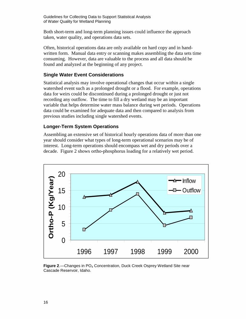
Longer-Term System Operations Assembling an extensive set of historical hourly operations data of more than one year should consider what types of long-term operational scenarios may be of interest. Long-term operations should encompass wet and dry periods over a decade. Figure 2 shows ortho-phosphorus loading for a relatively wet period.
Figure 2.—Changes in PO4 Concentration, Duck Creek Osprey Wetland Site near Cascade Reservoir, Idaho.
0
5
10
15
20
1996 1997 1998 1999 2000
Ort
ho-P
(Kg/
Yea
r) InflowOutflow
Develop the Sample Analysis Plan
17
Water Quality
Wetland water quality empirical modeling requires combined inflow (total upstream inflow to wetland above weir) data in the wetland, measured boundary input data (at the inflow edges of the wetland), and outflow data (at the weir). At a minimum, the following additional meta data are to be collected along with the water quality data:
The sampling location GPS coordinates (or distance) along the wetland (from inflow points to outlet).
• Flow at sampling point (if any), air temperature, water temperature, names
of data collectors, cloud cover conditions, maps used, and surrounding agricultural conditions.
• Water elevation stage data at the weir outlet water quality sampling location and other within-the-wetland data.
One-unit natural wetlands are most common. This means that aerobic degradation of BOD, nitrification, denitrification, fixation of phosphorus, and other processes occur in the same less-optimal reactor resulting in lack of control and regulation of processes (Moshiri, 1993).
Wetland systems process both particulate (refractory) and dissolved (labile) organic matter. Biochemical oxygen demand (BOD) removal is by both physical and microbial processes in the wetland. BOD has both nitrogenous and carbonaceous components that consume oxygen. This lumped parameter often becomes a critical water quality indicator. Due to slow water velocities and long
residence time in wetlands, suspended solids (SS) settle and are retained. These non-specific lumped parameters, specifically the 5-day BOD and total SS are often used in wetland design equations.
Chemical oxygen demand (COD) is the amount of chemical oxidant required to oxidize organic matter. In the wetland environment with large amounts of humic matter, COD values are much higher than BOD values. Total organic carbon (TOC) is also typically larger than BOD.
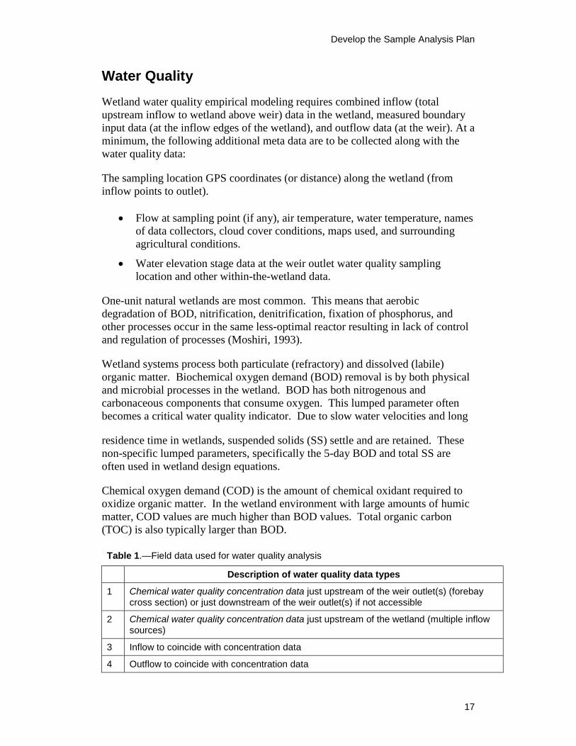
Table 1.—Field data used for water quality analysis
Description of water quality data types
1 Chemical water quality concentration data just upstream of the weir outlet(s) (forebay cross section) or just downstream of the weir outlet(s) if not accessible
2 Chemical water quality concentration data just upstream of the wetland (multiple inflow sources)
3 Inflow to coincide with concentration data
4 Outflow to coincide with concentration data
Guidelines for Collecting Data to Support Statistical Analysis of Water Quality for Wetland Planning
18
Changes in total dissolved solids (TDS) concentration in wetlands are usually not significant. However, TDS which is an indicator of salt in the water is typically used as a general indicator of water quality and is generally collected.
Wetlands designed for ammonia (NH4-N), a compound toxic to aquatic organisms, or nitrate (NO3-N) removal need a complete understanding of the nitrogen budget as well as the total nutrient budget. Ammonia removal, and thus nitrification, is related to HRT. Nitrate is removed by both plant uptake as a nutrient and by denitrification (Wetzel, 2001). In general, wetlands tend to sequester nutrients. However, wetlands that are drained and then later reestablished on the same site, can release nutrients. An example, is a dried out peat wetland; upon wetting such a wetland, phosphorus tends to be released.
Based on the Cascade report (Bureau of Reclamation, December 2003) the following typical water parameters are collected:
• Nitrogen components • Phosphorus components • Turbidity and suspended sediment components • Effects of organics (BOD5)
Mnemonic definitions:
BODu Ultimate carbonaceous biochemical oxygen demand (mg/L)
BOD-5 5-day biochemical oxygen demand (mg/L)
DO Dissolved oxygen concentration (mg/L) Tw Wetland open water temperature (°C)
TSS Total suspended solids (mg/L)
TDS Total dissolved solids (mg/L)
DO process rates are physical and biochemical processes that affect the DO levels, normalized by mean depth to units of gO2/m2/day
Temperature Data Collection and Processing Water temperature data are typically more extensive than water quality data records. Some historical wetland water quality data may be available from previous studies.
Temperature and Water Quality Data Used in Statistical Model Linear-regression statistical analyses might initially be done to examine distributions and during data assemblage to identify trends.
Develop the Sample Analysis Plan
19
Existing Water Quality Data Sources and Monitoring Although wetland studies focus on wastewater data, other types of model development and data sources should be considered when collecting data. Existing wetland databases at other nearby sites may often be the only available historical data for a wetland study. Continuous monitoring at a nearby wetland site can provide clues to explaining study site conditions.
Water Quality Data Gaps and Data Development Considerations Existing historical data may be adequate for initial cursory analysis. Analysis of other data sources, including new continuous thermistor data, could help in confirming data sets and in providing a reference in applying data sets to previous years. Additional considerations include:
• Accommodating special hydraulic situations.
• Evaluating potential action alternatives associated with ongoing basin water use planning and evaluating wetland modeling priorities, water quality parameters, and other requirements.
• Cooperation between participants who have technical expertise in water quality modeling, ecology, and fisheries.
Water Quality Data Collection and Processing Data must be processed and archived in an electronic format that is readily available for future statistical analysis. Meta data and other field notes should be archived in databases. Some information for analysis may need to be estimated rather than measured.
Wetland Vegetation
As described under Major Wetland Functions, vegetation plays important roles in wetland treatment processes so it is important to sample vegetation for quantifying overall wetland health and treatment function (Thullen et al., 2005 and Thullen, et al., 2002). Vegetation growth can affect water flow paths, nutrient processing, as well as wildlife habitats. Wetland vegetation including periphyton (attached algae) and floating aquatic vegetation are important components.
The oxygen leakage from roots provides oxidized conditions in anoxic soils that stimulate aerobic decomposition of organic matter and growth of nitrifying bacteria (Moshiri, 1993). Additionally, wetland vegetation provides the substrate for the attached bacteria and algae (periphyton), shade and filtering capability for reducing TSS, uptake of nutrients and other constituents, the ability to pull NO3 down into anaerobic zones as it absorbs water, and upon dying, provides a carbon source for the denitrifying bacteria (Kadlec and Wallace, 2009; Martin and Wool, 2002, Mitsch and Gosselink, 2000).
Guidelines for Collecting Data to Support Statistical Analysis of Water Quality for Wetland Planning
20
Dead plant stems, or culms, can be harvested to remove carbon and nutrients tied up in the biomass. For example, in pot-hole regions, wetlands need to dry out before lake hay can be harvested for livestock. If a control structure such as an outlet weir can be lowered during a dry hydrologic cycle, haying can occur on a more scheduled basis to harvest hay from the edges of the wetland. For open water areas, mechanical weed harvesters could be used to remove submerged and floating vegetation up to a depth of 5 to 7 feet; harvested waste could be used for compost. However, harvesters are not used to remove large emergent, wetland plants, such as cattails.
Burning cattails and bulrush as needed can reduce vegetative buildup within a wetland, stimulate fresh new growth following re-flooding, reduce mosquito breeding habitat, and can re-oxygenate the area. However, in addition to contributing to air quality issues, burning can leave residual ash which contributes to a spike in carbon and nutrient release from the first flush after re-flooding. Vegetation establishment in a wetland is more of an art than a science and often requires a bit of luck. Wetland plants can be killed by insufficient soil moisture (site dries out), excessive water depths (flooding at the site), plant damage, insect infestation, inadequate soil preparation, incorrect planting methods, incorrect time of planting, wildlife predation, and other factors.
Sampling of aquatic vegetation therefore includes identifying plant species, measuring biomass, plant density, coverage, uptake of nutrients and other constituents, wildlife use, and detrital buildup and decomposition. While there is not a huge number of plant species used in constructed wetlands, many are very difficult to discern from one another. The various species have different growth needs so knowing the correct species that are present as well as the ones being planted is critical for success. Good references for species identification depend upon the region. However, for much of Reclamation’s jurisdiction, Correll, D.S. and Correll, H.B. (1975), Aquatic and Wetland Plants of Southwestern United States, Stanford University Press, Stanford, CA, Volumes I and II, ISBN 0-8047-0866-5, 1777 pp., is excellent for identification even if some of the genus names have changed.
For Colorado wetlands, Culver, Denise R. and Lemly, Joanna M., 2013, “Field Guide to Colorado’s Wetland Plants, Identification, Ecology, and Conservation,” Prepared for the U.S. Environmental Protection Agency (EPA) by the Colorado Natural Heritage Program, Warner College of Natural Resources, Colorado State University, Fort Collins, CO, ISBN: 978-0-615-74649-4, printed by Vision Graphics, Inc., Loveland, Colorado is an excellent choice. Additionally, there are a number of good online sources with photographs available to help identify wetland plant species. Determining whether plant biomass, density, or coverage data are most useful depends upon the goals of the project. Often areal coverage is easiest, especially if the wetland is large and geo-rectified aerial photographs can be obtained of the site. Area covered by the vegetation species can then be measured using ArcGIS
Develop the Sample Analysis Plan
21
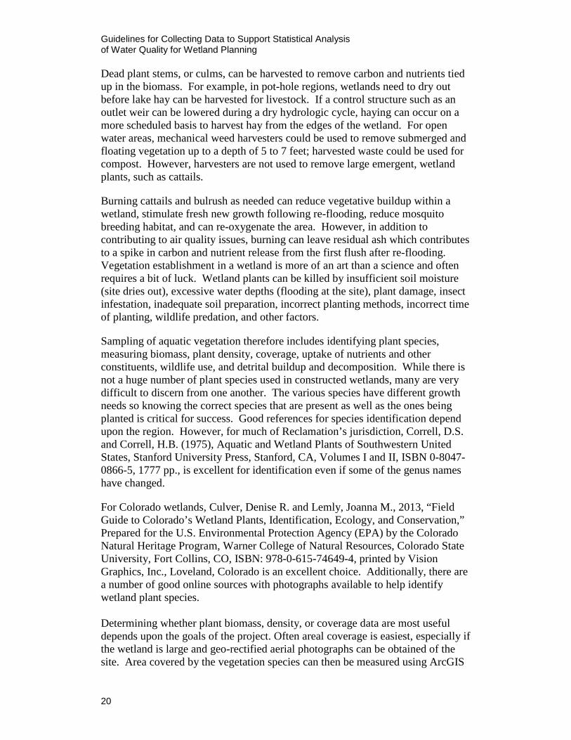
mapping. If more specific information is required regarding the vegetation, then biomass and/or density measurements are justified. Methods are described in Daniels et al. (2010) and Sartoris et al. (2000a, 200b). Figure 3 illustrates the biomass sample collection point.
Figure 3.—Schoenoplectus americanus (Olney’s bulrush) biomass cut at soil line from a randomly placed 0.25-m2 quadrat. Sample will be dried and weighed for biomass as grams per square meter. Density is the number of culms (stems) within the quadrat, reported as number of culms per square meter. Culm diameter and length can also be important in evaluating health. Elemental analyses of vegetation is necessary to evaluate some projects and it is as important to collect the sample material according to protocol as it is to have the samples analyzed according to acceptable standards. Examples of analyses often performed include, total nitrogen, phosphorus, potassium, carbon, selenium, arsenic, mercury, ash, and other constituents of importance to the specific projects. Standardized methods of plant tissue analyses are critical in order to compare results reported in the literature, among various locations, and over time. Plant litter buildup over time can drastically affect how a wetland functions (Sartoris et al., 2000a, 2000b). Evaluating the water quality of the system can determine whether the buildup negatively impacts the system and to what extent. Wildlife use is expected (see following sections) but can sometimes be so abundant that over use can negatively affect the growth and survival of the
Guidelines for Collecting Data to Support Statistical Analysis of Water Quality for Wetland Planning
22
vegetation as they pull out newly planted plants, chew off new shoots to the water line, and mat down emergent vegetation preventing new growth. Depending again upon the project goals as well as the extent of the damage, will determine how best to negate the impact or manage the wetland.
Aquatic Biota
Bacteria, phytoplankton, zooplankton, and macro-invertebrates are also extremely important to the proper functioning of wetlands and therefore need to be considered during wetland design. As mentioned earlier, nitrifying and denitrifying bacteria perform the nitrogen transformations; phytoplankton and periphyton are important in nutrient and other constituent uptake processes, as well as oxidizing the water column, and providing food for zooplankton, macr0-invertebrates and wildlife. Macro-invertebrates aid in plant decomposition, mosquito control and provide food for wildlife (Thullen et al., 2008). Plankton and macro-invertebrates can be sampled for enumeration and species identification to quantify wetland productivity, and monitored for toxic or noxious species. Algal blooms can be caused by improper hydraulics or loading rates and can cause wildlife disease outbreaks or drops in dissolved oxygen during massive algal die-offs.
Birds (Swimming, Diving, and Nesting)
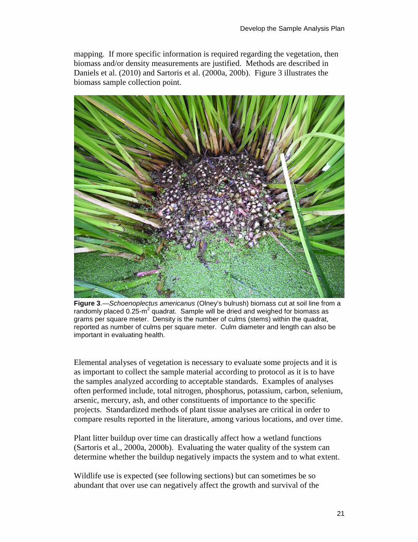
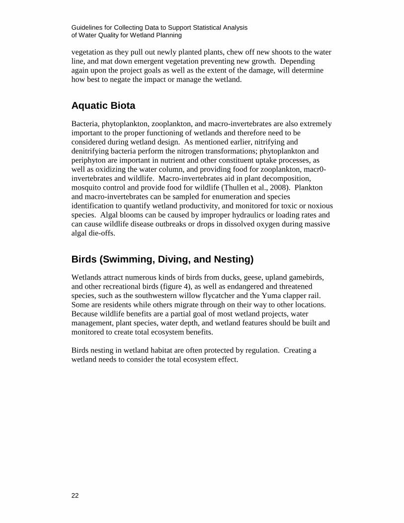
Wetlands attract numerous kinds of birds from ducks, geese, upland gamebirds, and other recreational birds (figure 4), as well as endangered and threatened species, such as the southwestern willow flycatcher and the Yuma clapper rail. Some are residents while others migrate through on their way to other locations. Because wildlife benefits are a partial goal of most wetland projects, water management, plant species, water depth, and wetland features should be built and monitored to create total ecosystem benefits. Birds nesting in wetland habitat are often protected by regulation. Creating a wetland needs to consider the total ecosystem effect.
Develop the Sample Analysis Plan
23
Figure 4.—Duck wetland habitat within habitat used by blackbirds and other marsh birds.
Habitat and Regulations
Wetlands are habitat to many species including threatened and endangered species. Wetland habitats are protected and regulated by federal and state agencies. Section 404 of the Clean Water Act (CWA) regulates the discharge of dredged, excavated, or fill material in wetlands, streams, rivers, and other U.S. waters. The U.S. Army Corps of Engineers is the federal agency authorized to issue Section 404 Permits for certain activities conducted in wetlands or other U.S. waters.
CWA Section 402 establishes the National Pollutant Discharge Elimination System (NPDES) permit program to regulate point source discharges of pollutants into waters of the United States. An NPDES permit sets specific discharge limits for point sources discharging pollutants into waters of the United States and establishes monitoring and reporting requirements, as well as special conditions. EPA is charged with administering the NPDES permit program, but can authorize states to assume many of the permitting, administrative, and enforcement responsibilities of the NPDES permit program. Authorized states are prohibited from adopting standards that are less stringent than those established under the Federal NPDES permit program, but may adopt or enforce standards that are more stringent than the Federal standards if allowed under state law.
CWA Section 401 wetland certification protects wetlands from chemical and other types of alterations. Major permits subject to Section 401 of the CWA include section 402 and 404 permits.

Guidelines for Collecting Data to Support Statistical Analysis of Water Quality for Wetland Planning
24
Fish and Reptiles
The needs of fish and reptiles also have to be considered during wetland design. Wetlands can be designed specifically for the needs of the desired wetland species. This typically involves working with the specific wildlife species experts to get the correct design for the desired species.
Wetlands can be used to enhance fisheries, destroy nuisance fisheries, or to minimize impacts due to wetland creation. Wetlands can serve as cool thermal refugia for fish habitat or heat traps and fish winterkill locations depending on design. Several fish species, native and introduced, consume mosquito larvae and pupae. Often mosquito-fish are stocked to keep mosquito populations in check near populated areas. However, such introduced species can outcompete more desirable native species so local fishery biologists should be consulted prior to any fish introductions.
Snakes, alligators, and other dangerous reptiles need to be considered when designing wetlands, as well as other nuisance species such as nutria, pythons or quagga and zebra mussels. When creating or restoring wetlands, it is important to avoid creating future problems for nearby communities.
Aerial and Topographic Data
Aerial photography and associated image analysis was discussed by Mulamoottil, et al., 1996). The age and history of wetlands can be determined by examining photographs in chronological order in conjunction with hydrological history including floods and extended droughts.
Reference:
Mulamoottil, George, Warner, Barry G., and McBean, Edward A., 1996, “Wetlands, Environmental Gradients, Boundaries, and Buffers,” CRC Press, Inc., Boca Raton, Florida.
Wetland topography in the form of cross-sectional channel geometry is typically used to develop the volume elevation curve at water surface elevations during droughts. Inundated wetland conditions require more challenging methods of estimating geometry. The physical geometry of a wetland influences many associated wetland water quality processes. Wetlands with a large amount of open water have different characteristics than a wetland covered with dense vegetation.
Alternative Wetland Topographic Data Sources Cursory assessments with limited funding may use available cross-sectional channel geometry developed from topographic maps. However, this is typically not accurate enough due to contours being up to fifty percent off. Data taken
Develop the Sample Analysis Plan
25
during droughts provides valuable below-the-water-surface contour information during floods. Flown data, such as high precision three-dimensional (3D) Light Detection and Ranging (LiDAR) data, provides much better topographic information.
Meteorological Data
Meteorological data are an essential part of wetland temperature models. For example, the SPAW model is most sensitive to climatic data and less sensitive to crop and soil descriptions (Texas A&M and Bureau of Reclamation, 2008). Meteorological data provide the basis for coefficients applied in model equations affecting water quality. As a result, many technical factors are associated with the required meteorological data for those equations.
Hourly meteorological data are typically required due to large fluctuations in air temperature and solar radiation. There are often numerous National Weather Service (NWS), agricultural, and other nearby meteorological stations. Nearby stations can often be used to provide average hourly meteorological data and to fill in data gaps. However, a meteorological probe near the edge of the wetland is preferred.
Meteorological Data for Statistical Analysis As a minimum, the following information is needed:
Meteorological data including: hourly drybulb (air) temperature (°C), dewpoint temperature (°C), windspeed (meters per second), solar radiation (kcal/m2/hr), barometric pressure (mb), and pan evaporation (cm). Meteorological data should be determined from the nearest meteorological station recording at 2 meters above the ground and close to the water surface elevation. For large wetlands more than one meteorological station may be used. Missing drybulb temperatures may be derived from maximum and minimum daily temperatures collected at a nearby AgriMet station. Accumulated precipitation and barometric pressure may also be collected at an AgriMet station.
Stations at a different elevation may not reflect water surface conditions. Airport stations tend to be far removed from the wetland site and could result in significant differences in wind, cloud cover, or solar radiation measurements from those at the study site.
Meteorological Station Installation To help resolve meteorological issues, new meteorological stations may need to be installed and maintained to provide a good reference for conditions for the wetland being studied. The stations might be installed through a cooperative effort and linked into a remote AgriMet monitoring network.
Guidelines for Collecting Data to Support Statistical Analysis of Water Quality for Wetland Planning
26
Wind speed reduced to near zero by riparian vegetation may increase water temperature. Riparian shading may decrease water temperature. Model calibration requires adequately representing the local conditions which are near the wetland. Hill top meteorological stations are often not representative of conditions at the wetland water surface.
Deploying Remote Stations and Collecting Field Data New meteorological data should be reviewed as soon as it comes in. New data will also provide an important reference for analyzing and adjusting historical meteorological data.
Meteorological station monitoring parameters should be defined to ensure that the data collected would meet the critical meteorological data needs for wetland data statistical analysis and use. Hourly data may be useful and could include the following:
• Hourly air and dew point temperatures
• Relative humidity - mean daily relative humidity can be converted to daily dewpoint temperature which can be an input required by some models
• Barometric pressure – hourly averages or determined from mean, minimum, and maximum records
Secondary priority parameters, such as pan evaporation, evapotranspiration, and wind run, can be estimated from data collected nearby. If nearby solar radiation was not collected for a historical calibration year, nearby cloud cover data might be used.
Meteorological Data Gaps and Model Considerations The following are recommendations for improved data sets for modeling wetlands.
• Examine data produced by new meteorological stations often to ensure proper function of equipment and proper QA/QC.
• Assess meteorological trends at other stations.
• Conduct a site visit to visually see if sampling and meteorological stations appear to be in representative locations.
Identify Upstream Boundary Conditions Upstream boundary conditions may be important to wetland analysis; therefore, it is important to select upstream wetland inflow locations where data is collected such as at a bridge, weir, or gage. Collect reconnaissance wetland inflow water
Identify Upstream Boundary Conditions
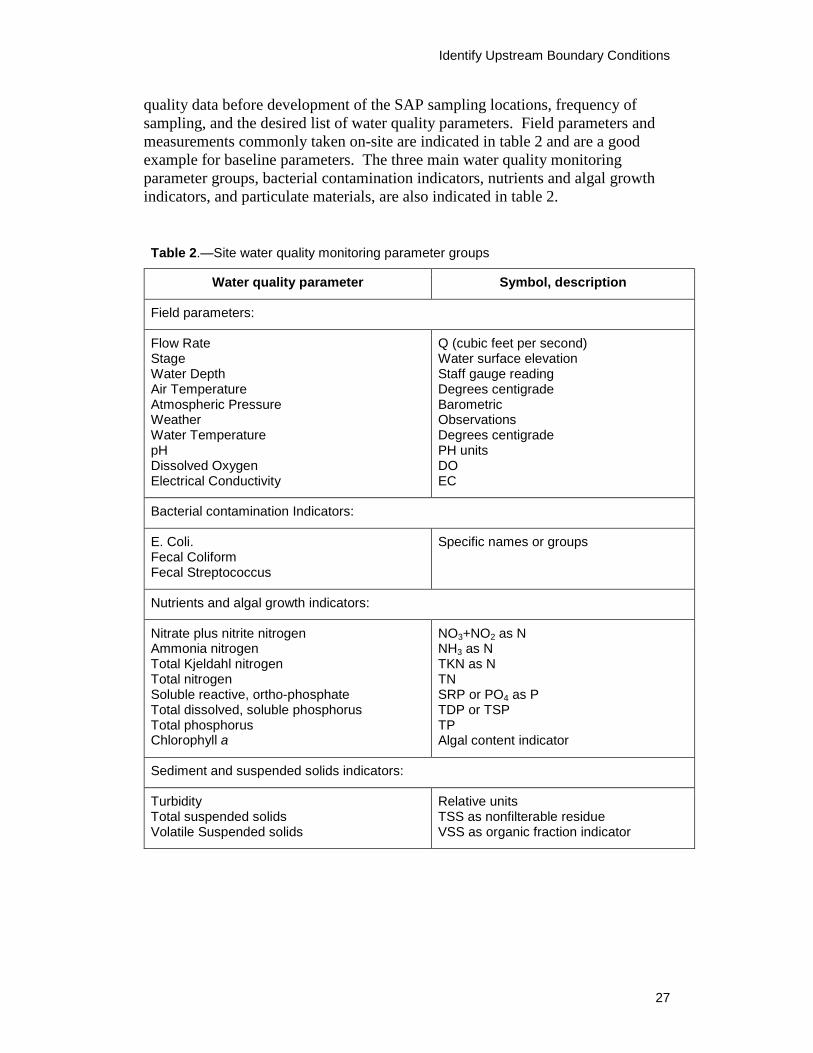
27
quality data before development of the SAP sampling locations, frequency of sampling, and the desired list of water quality parameters. Field parameters and measurements commonly taken on-site are indicated in table 2 and are a good example for baseline parameters. The three main water quality monitoring parameter groups, bacterial contamination indicators, nutrients and algal growth indicators, and particulate materials, are also indicated in table 2.
Table 2.—Site water quality monitoring parameter groups
Water quality parameter Symbol, description
Field parameters:
Flow Rate Stage Water Depth Air Temperature Atmospheric Pressure Weather Water Temperature pH Dissolved Oxygen Electrical Conductivity
Q (cubic feet per second) Water surface elevation Staff gauge reading Degrees centigrade Barometric Observations Degrees centigrade PH units DO EC
Bacterial contamination Indicators:
E. Coli. Fecal Coliform Fecal Streptococcus
Specific names or groups
Nutrients and algal growth indicators:
Nitrate plus nitrite nitrogen Ammonia nitrogen Total Kjeldahl nitrogen Total nitrogen Soluble reactive, ortho-phosphate Total dissolved, soluble phosphorus Total phosphorus Chlorophyll a
NO3+NO2 as N NH3 as N TKN as N TN SRP or PO4 as P TDP or TSP TP Algal content indicator
Sediment and suspended solids indicators:
Turbidity Total suspended solids Volatile Suspended solids
Relative units TSS as nonfilterable residue VSS as organic fraction indicator
Guidelines for Collecting Data to Support Statistical Analysis of Water Quality for Wetland Planning
28
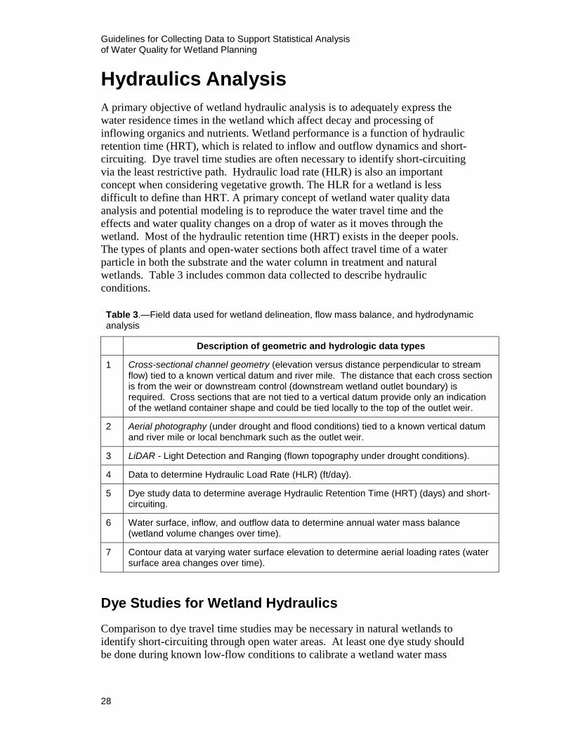
Hydraulics Analysis A primary objective of wetland hydraulic analysis is to adequately express the water residence times in the wetland which affect decay and processing of inflowing organics and nutrients. Wetland performance is a function of hydraulic retention time (HRT), which is related to inflow and outflow dynamics and short-circuiting. Dye travel time studies are often necessary to identify short-circuiting via the least restrictive path. Hydraulic load rate (HLR) is also an important concept when considering vegetative growth. The HLR for a wetland is less difficult to define than HRT. A primary concept of wetland water quality data analysis and potential modeling is to reproduce the water travel time and the effects and water quality changes on a drop of water as it moves through the wetland. Most of the hydraulic retention time (HRT) exists in the deeper pools. The types of plants and open-water sections both affect travel time of a water particle in both the substrate and the water column in treatment and natural wetlands. Table 3 includes common data collected to describe hydraulic conditions.
Table 3.—Field data used for wetland delineation, flow mass balance, and hydrodynamic analysis
Description of geometric and hydrologic data types
1 Cross-sectional channel geometry (elevation versus distance perpendicular to stream flow) tied to a known vertical datum and river mile. The distance that each cross section is from the weir or downstream control (downstream wetland outlet boundary) is required. Cross sections that are not tied to a vertical datum provide only an indication of the wetland container shape and could be tied locally to the top of the outlet weir.
2 Aerial photography (under drought and flood conditions) tied to a known vertical datum and river mile or local benchmark such as the outlet weir.
3 LiDAR - Light Detection and Ranging (flown topography under drought conditions).
4 Data to determine Hydraulic Load Rate (HLR) (ft/day).
5 Dye study data to determine average Hydraulic Retention Time (HRT) (days) and short- circuiting.
6 Water surface, inflow, and outflow data to determine annual water mass balance (wetland volume changes over time).
7 Contour data at varying water surface elevation to determine aerial loading rates (water surface area changes over time).
Dye Studies for Wetland Hydraulics
Comparison to dye travel time studies may be necessary in natural wetlands to identify short-circuiting through open water areas. At least one dye study should be done during known low-flow conditions to calibrate a wetland water mass
Hydraulics Analysis
29
balance. Rhodomine WT dye (red) or fluorine (yellow) florescent dye can be read with a fluorometer. Red dye in the wetland can alert the public and therefore yellow dye is typically used if the water travel time dye study cannot be done at night. However, fluorimetric dyes are notorious for being adsorbed or degraded during passage through a wetland resulting in failure to recover 100 percent of the dye. Dye studies mimic the tracking of a water particle downstream and indicate water travel time of a drop of water traveling through the shortest wetland path from the inflow to the outlet; failure to recover the majority of the dye mass may indicate dye collecting in stagnant areas of the wetland. Typically other model input data, such as flow, temperatures, and meteorology are also collected at the time of the dye study for empirical model development. Low-pool data sets following a dry period are preferred for water quality analysis.
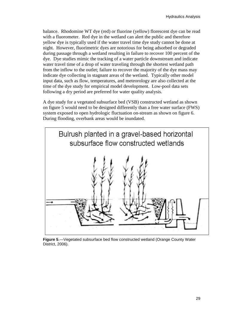
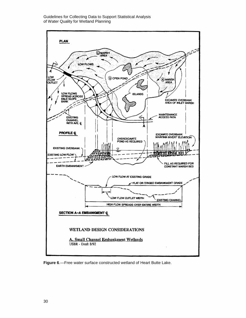
A dye study for a vegetated subsurface bed (VSB) constructed wetland as shown on figure 5 would need to be designed differently than a free water surface (FWS) system exposed to open hydrologic fluctuation on-stream as shown on figure 6. During flooding, overbank areas would be inundated.
Figure 5.—Vegetated subsurface bed flow constructed wetland (Orange County Water District, 2006).
Guidelines for Collecting Data to Support Statistical Analysis of Water Quality for Wetland Planning
30
Figure 6.—Free water surface constructed wetland of Heart Butte Lake.
Hydraulics Analysis
31
HLR and HRT Analysis
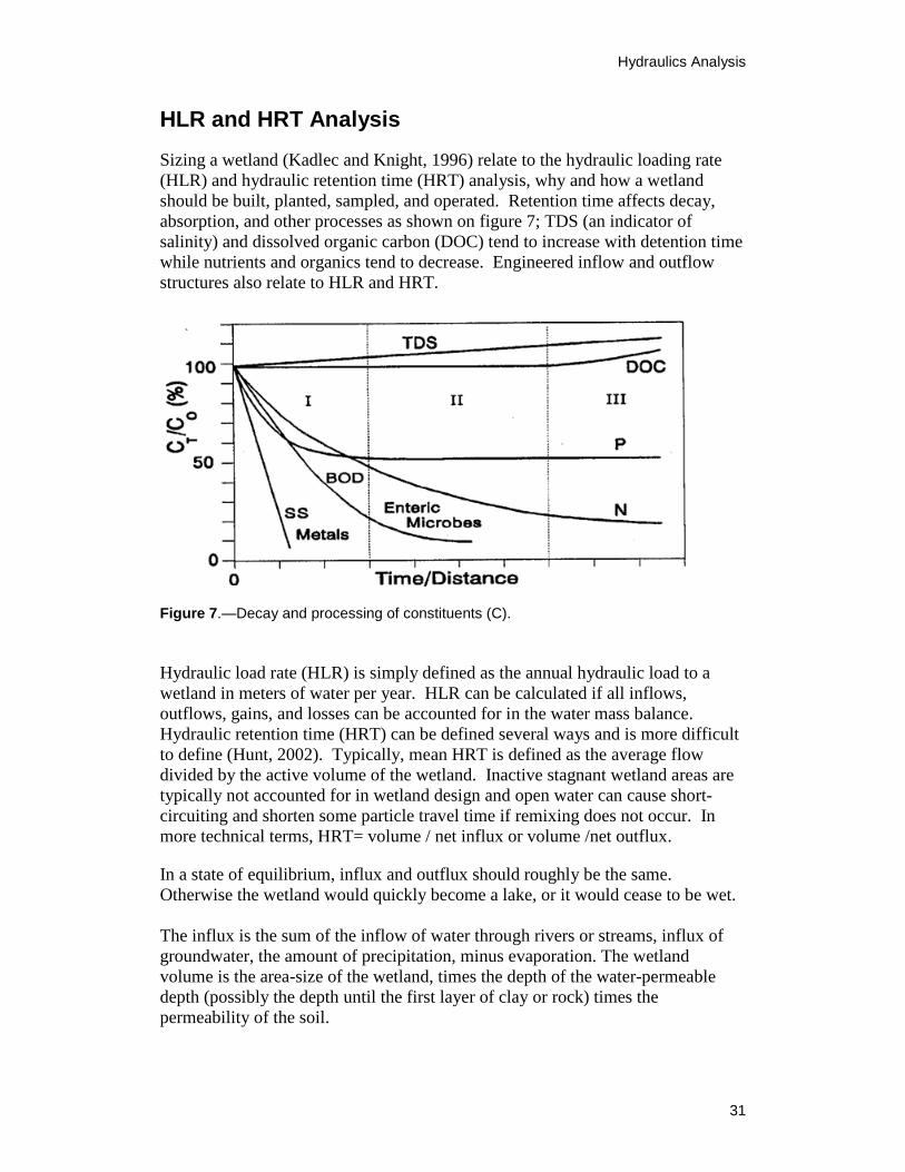
Sizing a wetland (Kadlec and Knight, 1996) relate to the hydraulic loading rate (HLR) and hydraulic retention time (HRT) analysis, why and how a wetland should be built, planted, sampled, and operated. Retention time affects decay, absorption, and other processes as shown on figure 7; TDS (an indicator of salinity) and dissolved organic carbon (DOC) tend to increase with detention time while nutrients and organics tend to decrease. Engineered inflow and outflow structures also relate to HLR and HRT.
Figure 7.—Decay and processing of constituents (C). Hydraulic load rate (HLR) is simply defined as the annual hydraulic load to a wetland in meters of water per year. HLR can be calculated if all inflows, outflows, gains, and losses can be accounted for in the water mass balance. Hydraulic retention time (HRT) can be defined several ways and is more difficult to define (Hunt, 2002). Typically, mean HRT is defined as the average flow divided by the active volume of the wetland. Inactive stagnant wetland areas are typically not accounted for in wetland design and open water can cause short-circuiting and shorten some particle travel time if remixing does not occur. In more technical terms, HRT= volume / net influx or volume /net outflux.
In a state of equilibrium, influx and outflux should roughly be the same. Otherwise the wetland would quickly become a lake, or it would cease to be wet. The influx is the sum of the inflow of water through rivers or streams, influx of groundwater, the amount of precipitation, minus evaporation. The wetland volume is the area-size of the wetland, times the depth of the water-permeable depth (possibly the depth until the first layer of clay or rock) times the permeability of the soil.
Guidelines for Collecting Data to Support Statistical Analysis of Water Quality for Wetland Planning
32
Wetland empirical models are constructed from available bathymetric or topographic data representing the physical configuration and measured data sets that represent transient operational, hydraulic, meteorological, and water quality conditions. Future wetland analysis could be based on refining an existing equation or improving existing data sets.
Flows and Water Mass Balance Data
Data representing major water inputs and losses from the system are required for wetland analysis. This refers mainly to flow and stage data, because precipitation, seepage, and evaporation are reflected in the local drainage flow and stage gages.
Field personnel who maintain the gages and collect the data should be trained in data processing, should process the data in a timely manner to adjust inconsistencies or explain data gaps, and should also record metadata such as weather conditions during data collection.
Typical mistakes include collecting river temperatures in eddies and other slow- moving backwater areas not representative of complete mixed conditions.
Boundary conditions should encompass the characteristics of the local drainage area and should not be influenced by inundation including groundwater inundation effects.
Wetland Water Mass Balance Data Sources
The methodology for a water mass balance should be tailored to known inflow, outflow, and volume information. Inflow from ungauged tributaries will need to be estimated for wet, average, and dry conditions.
Flow Monitoring and Data Compilation
Wetland models are ideally calibrated to data sets representing low and high pool conditions to improve the accuracy of simulations made over a wide range of conditions. Historic flow records should be reviewed and compiled to find a sufficient range of data for the expected applications.
Water Budget Data Gaps and Empirical Model Considerations
Long-term flow records for wetland and tributary gauging stations are generally more complete than corresponding water quality data records. Some considerations include:
Hydraulics Analysis
33
• Scenarios or action alternatives to be investigated.
• Collect flow measurements or compare to already collected measurements such as Acoustic Doppler Current Profiler (ADCP) measurements at key cross section locations to estimate water gains and losses per inflow area.
• Evaluate system wide operational flow data to determine if changes, such as delayed filling or diking practices in recent years, have also resulted in new trends in wetland water quality conditions. First flush effects from nonpoint sources after a rainstorm need to be considered also.
Hydrodynamics and Short-circuiting
Water entering a wetland open water area can short-circuit to the outlet in a short amount of time. Hummicks placed in open areas remix the water column. Hummicks influence hydraulic performance (Keefe, et al., 2010). Wetland hydraulics of interest includes the following:
• Water (dye particle) travel times • Number and routing path of inflows • Stagnant areas
Various graphic display options are available using post-processor programs to display output and statistics. Plotting and statistical options show the strengths and capability of empirical models. Plotting of both empirical model and field data may be possible.
Some of the plot options for reporting output could include the following:
• Stage versus time • Mean water depth versus distance • Diurnal variations in water quality parameters • Water quality parameter inflow and outflow wetland loadings • Seasonal or annual fluctuations under dry and wet conditions
And hydrodynamics, especially short-circuiting, affects wetland water quality, the collection of data for water quality analysis, and ultimately final wetland design.
Cross-sectional Channel Geometry Survey Methods
Accurate geometric surveys include a below-the-water surface representation of the wetland bottom. Cross-sectional channel sections near the outlet controls are needed. Real Time Kinetic (RTK) survey measurements from a boat might not be feasible for relatively flat wetland terrain. Therefore manual survey methods are typically used around the edges of wetlands. Topographic maps might be used if
Guidelines for Collecting Data to Support Statistical Analysis of Water Quality for Wetland Planning
34
less accuracy is adequate. If more accuracy is desired, LIDAR measurements might be taken. However, submerged areas will be problematic.
The primary purpose of a cross-sectional channel survey is for developing modeling geometry, to identify major hydraulic controls, and to baseline wetland depressions of interest. The time of each surveyed cross section should be recorded along with the bottom depth from the water surface at that time. Ferrari and Collins (2006) cover survey and data analysis methods.
Digital Mapping Data Format and Processing
All elevations need to be tied to a common vertical datum, which is usually chosen as “project datum” or the commonly used North American Vertical Datum of 1988 (NAVD88). Multiple maps should have a common horizontal datum also to tie maps together.
To minimize confusion when presenting results it may be necessary to represent distances from a known location. For example, it is more understandable to report results at 0.5 miles upstream of the outlet control weir rather than in GPS coordinates.
Grid Considerations
How physical geometry is converted into computational segments for modeling depends partly on available data, model approach, and professional judgment. The horizontal layout (plan view) should include inflow and outflow considerations, structures affecting water level, and water depths. Connectivity between wetlands should consider potential groundwater flow paths. Layout should also take into account future wetlands as potential mitigation for lost wetlands. Hummocks within a wetland can affect minor and major transport corridors by mixing flow; hummocks affect vertical and horizontal mixing and stratification in wetlands. As wetlands change over time due to vegetative growth, wetland compartment flow dynamics can change resulting in a difficult hydrodynamic modeling challenge. Therefore modeling is typically simplified to flow and water mass balances.
Selecting Sampling Locations
35
Selecting Sampling Locations The sampling protocol for the selected analysis (such as the wetland locations, bridge and weir locations, and segments) should be identified early. Data collection layout should be carefully considered before data collection; it is how wetlands are constructed that makes them effective at water treatment. A common mistake is to place a gage or collect samples in a recirculation eddy, backwater area, or in a location where solar radiation directly shines on a thermistor. Samples that are representative of a completely-mixed plug-flow condition should be collected. If stratification occurs in wetland pools, vertical water quality profiles over depth may be necessary. Hyporheic groundwater inflow may produce lateral gradients across the wetland and thermal refugia; data may need to be collected laterally on each side of the main flow path through the wetland.
The following sketches (figures 8, 9, and 10) show the type of zones at the Tres Rios Demonstration Wetland site. Sampling collection sites (figure 8) are affected by hummocks (figure 8) which alter flow paths and wetland zones.
An entirely different configuration was used at the Sac and Fox site on figure 11. Notice the horizontal flow arrows which show the lengthened flow path around dikes to increase water residence time and efficiency of processing wastewater discharges. Nearly every wetland configuration is unique. Planning specifics for each site are critical. A way to avoid compounding errors is to study the wetland site configuration and sketch potential layouts for enhancement of the wetland.
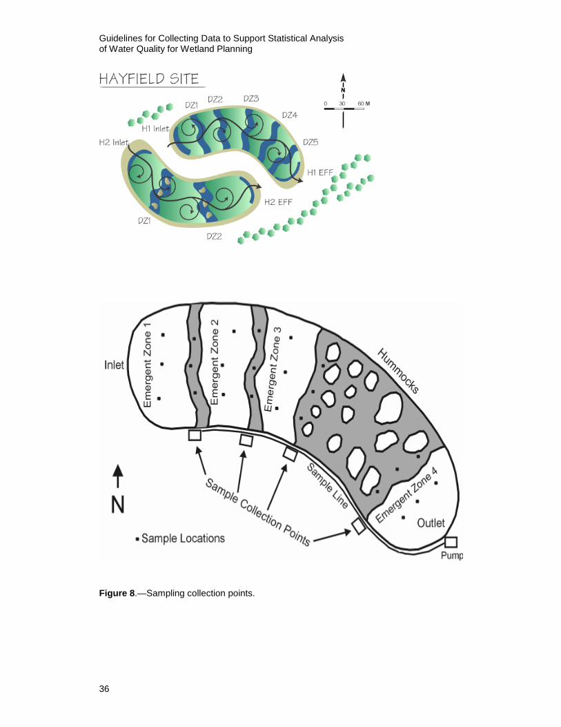
Guidelines for Collecting Data to Support Statistical Analysis of Water Quality for Wetland Planning
36
Figure 8.—Sampling collection points.
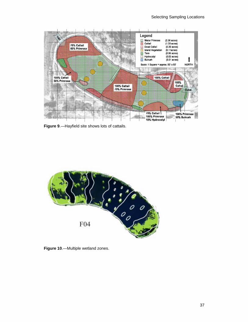
Selecting Sampling Locations
37
Figure 9.—Hayfield site shows lots of cattails.
Figure 10.—Multiple wetland zones.
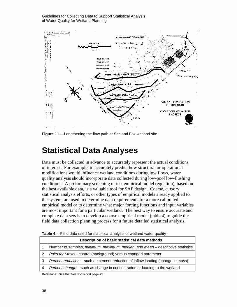
Guidelines for Collecting Data to Support Statistical Analysis of Water Quality for Wetland Planning
38
Figure 11.—Lengthening the flow path at Sac and Fox wetland site.
Statistical Data Analyses Data must be collected in advance to accurately represent the actual conditions of interest. For example, to accurately predict how structural or operational modifications would influence wetland conditions during low flows, water quality analysis should incorporate data collected during low-pool low-flushing conditions. A preliminary screening or test empirical model (equation), based on the best available data, is a valuable tool for SAP design. Coarse, cursory statistical analysis efforts, or other types of empirical models already applied to the system, are used to determine data requirements for a more calibrated empirical model or to determine what major forcing functions and input variables are most important for a particular wetland. The best way to ensure accurate and complete data sets is to develop a coarse empirical model (table 4) to guide the field data collection planning process for a future detailed statistical analysis. Table 4.—Field data used for statistical analysis of wetland water quality
Description of basic statistical data methods
1 Number of samples, minimum, maximum, median, and mean – descriptive statistics
2 Pairs for t-tests - control (background) versus changed parameter
3 Percent reduction - such as percent reduction of inflow loading (change in mass)
4 Percent change - such as change in concentration or loading to the wetland Reference: See the Tres Rio report page 75.
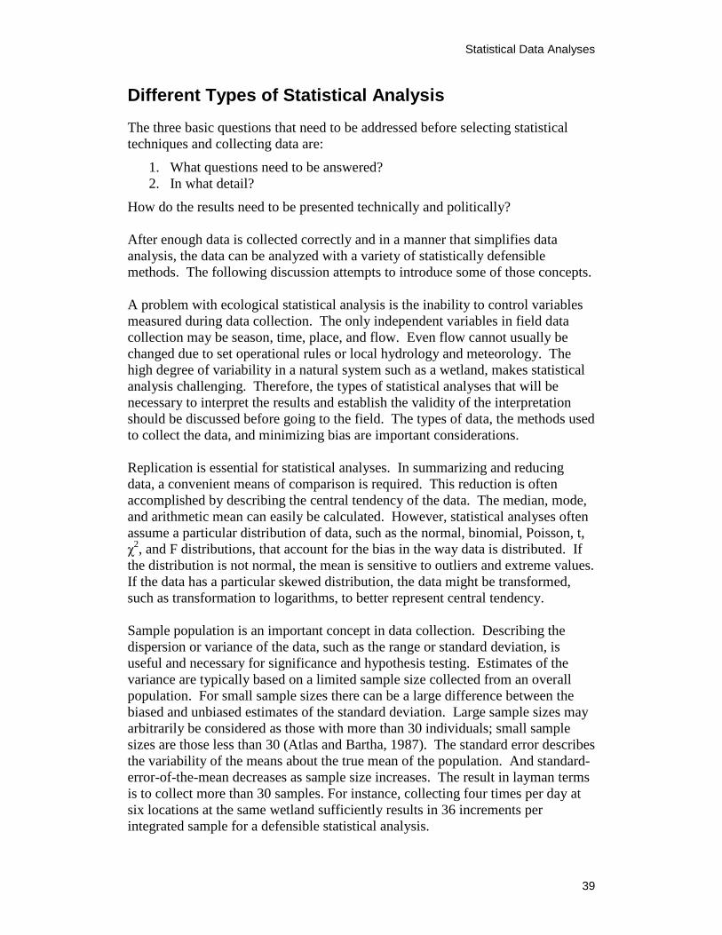
Statistical Data Analyses
39
Different Types of Statistical Analysis
The three basic questions that need to be addressed before selecting statistical techniques and collecting data are:
1. What questions need to be answered? 2. In what detail?
How do the results need to be presented technically and politically? After enough data is collected correctly and in a manner that simplifies data analysis, the data can be analyzed with a variety of statistically defensible methods. The following discussion attempts to introduce some of those concepts. A problem with ecological statistical analysis is the inability to control variables measured during data collection. The only independent variables in field data collection may be season, time, place, and flow. Even flow cannot usually be changed due to set operational rules or local hydrology and meteorology. The high degree of variability in a natural system such as a wetland, makes statistical analysis challenging. Therefore, the types of statistical analyses that will be necessary to interpret the results and establish the validity of the interpretation should be discussed before going to the field. The types of data, the methods used to collect the data, and minimizing bias are important considerations. Replication is essential for statistical analyses. In summarizing and reducing data, a convenient means of comparison is required. This reduction is often accomplished by describing the central tendency of the data. The median, mode, and arithmetic mean can easily be calculated. However, statistical analyses often assume a particular distribution of data, such as the normal, binomial, Poisson, t, χ2, and F distributions, that account for the bias in the way data is distributed. If the distribution is not normal, the mean is sensitive to outliers and extreme values. If the data has a particular skewed distribution, the data might be transformed, such as transformation to logarithms, to better represent central tendency. Sample population is an important concept in data collection. Describing the dispersion or variance of the data, such as the range or standard deviation, is useful and necessary for significance and hypothesis testing. Estimates of the variance are typically based on a limited sample size collected from an overall population. For small sample sizes there can be a large difference between the biased and unbiased estimates of the standard deviation. Large sample sizes may arbitrarily be considered as those with more than 30 individuals; small sample sizes are those less than 30 (Atlas and Bartha, 1987). The standard error describes the variability of the means about the true mean of the population. And standard-error-of-the-mean decreases as sample size increases. The result in layman terms is to collect more than 30 samples. For instance, collecting four times per day at six locations at the same wetland sufficiently results in 36 increments per integrated sample for a defensible statistical analysis.
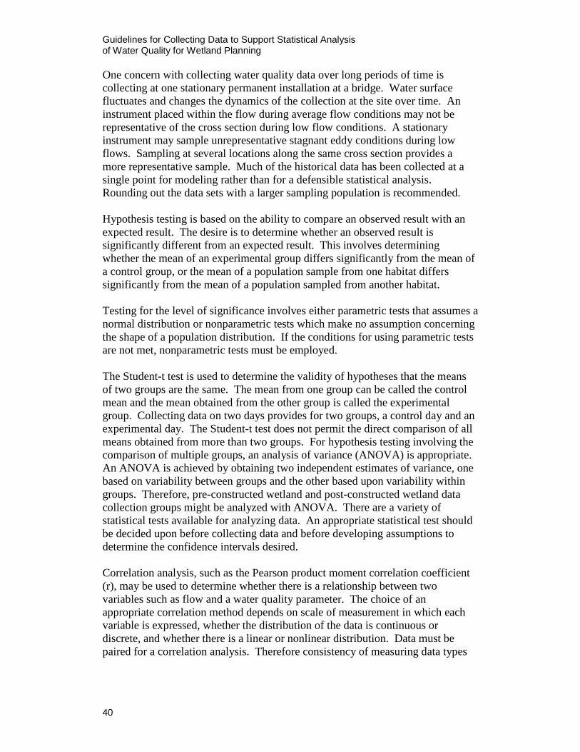
Guidelines for Collecting Data to Support Statistical Analysis of Water Quality for Wetland Planning
40
One concern with collecting water quality data over long periods of time is collecting at one stationary permanent installation at a bridge. Water surface fluctuates and changes the dynamics of the collection at the site over time. An instrument placed within the flow during average flow conditions may not be representative of the cross section during low flow conditions. A stationary instrument may sample unrepresentative stagnant eddy conditions during low flows. Sampling at several locations along the same cross section provides a more representative sample. Much of the historical data has been collected at a single point for modeling rather than for a defensible statistical analysis. Rounding out the data sets with a larger sampling population is recommended. Hypothesis testing is based on the ability to compare an observed result with an expected result. The desire is to determine whether an observed result is significantly different from an expected result. This involves determining whether the mean of an experimental group differs significantly from the mean of a control group, or the mean of a population sample from one habitat differs significantly from the mean of a population sampled from another habitat. Testing for the level of significance involves either parametric tests that assumes a normal distribution or nonparametric tests which make no assumption concerning the shape of a population distribution. If the conditions for using parametric tests are not met, nonparametric tests must be employed. The Student-t test is used to determine the validity of hypotheses that the means of two groups are the same. The mean from one group can be called the control mean and the mean obtained from the other group is called the experimental group. Collecting data on two days provides for two groups, a control day and an experimental day. The Student-t test does not permit the direct comparison of all means obtained from more than two groups. For hypothesis testing involving the comparison of multiple groups, an analysis of variance (ANOVA) is appropriate. An ANOVA is achieved by obtaining two independent estimates of variance, one based on variability between groups and the other based upon variability within groups. Therefore, pre-constructed wetland and post-constructed wetland data collection groups might be analyzed with ANOVA. There are a variety of statistical tests available for analyzing data. An appropriate statistical test should be decided upon before collecting data and before developing assumptions to determine the confidence intervals desired. Correlation analysis, such as the Pearson product moment correlation coefficient (r), may be used to determine whether there is a relationship between two variables such as flow and a water quality parameter. The choice of an appropriate correlation method depends on scale of measurement in which each variable is expressed, whether the distribution of the data is continuous or discrete, and whether there is a linear or nonlinear distribution. Data must be paired for a correlation analysis. Therefore consistency of measuring data types
Statistical Data Analyses
41
and frequency is encouraged and a clearly defined sampling protocol should be followed now and in the distant future. If there is a true independent variable, such as flow through the wetland, a mathematical relationship between the two variables, such as a linear regression analysis, might be attempted. Sometimes a positive correlation does not establish a cause and effect relation. In regression analysis, a relationship of best fit is used to describe the data. Transformation of the data might be required to develop a linear relationship in this parametric approach. However, untransformed data and nonparametric analyses might be more useful. In addition, previous data analysis might provide valuable information during additional statistical analysis of the data. Cluster analysis is an extension of correlation analysis that might be used to understand the distribution of populations in the natural habitat. Cluster analysis methods permit grouping of variables, such as multiple algal types, according to the magnitudes and interrelationships of their correlation or similarity coefficients. After establishing a correlation or similarity matrix, association coefficients might be attempted. The ability to utilize quantitative information to calculate a single similarity coefficient for comparisons may be useful. A single coefficient that permits mixing types of data allow for ecological analysis that contain the quantitative data normally obtained from the measurement of parameters such as temperature, TDS, pH, and nutrient concentrations; enumeration data of biological populations, such as number of algae; and microbial data such as respiration rates and nitrogen fixation rates. Unlike cluster analysis, where there is no direct expressed understanding of why variables cluster together, factor analysis aims to identify underlying factors behind correlations. Factor analysis allows for resolving complex relationships into the interaction of fewer and simpler factors such as environmental variables in the ecosystem. Principal “component” analysis and principal “factor” analysis are two methods of factor analysis. Principal component analysis features are uncorrelated; in principal factor analysis it is assumed that some features are correlated with others. A system-wide approach to data collection must be kept in mind because data collected could be used in models in future studies. Table 5 lists some typical statistical methods that might be used to answer different questions. The statistical methods in table 5 are just some examples of the available techniques and distributions.
Statistics are used in both hydrodynamic and water quality analysis as will be discussed in the next sections.
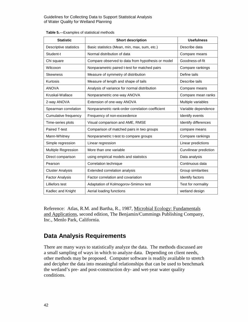
Guidelines for Collecting Data to Support Statistical Analysis of Water Quality for Wetland Planning
42
Table 5.—Examples of statistical methods
Statistic Short description Usefulness
Descriptive statistics Basic statistics (Mean, min, max, sum, etc.) Describe data
Student-t Normal distribution of data Compare means
Chi square Compare observed to data from hypothesis or model Goodness-of-fit
Wilcoxon Nonparametric paired t-test for matched pairs Compare rankings
Skewness Measure of symmetry of distribution Define tails
Kurtosis Measure of length and shape of tails Describe tails
ANOVA Analysis of variance for normal distribution Compare means
Kruskal-Wallace Nonparametric one-way ANOVA Compare mean ranks
2-way ANOVA Extension of one-way ANOVA Multiple variables
Spearman correlation Nonparametric rank-order correlation coefficient Variable dependence
Cumulative frequency Frequency of non-exceedence Identify events
Time-series plots Visual comparison and AME, RMSE Identify differences
Paired T-test Comparison of matched pairs in two groups compare means
Mann-Whitney Nonparametric t-test to compare groups Compare rankings
Simple regression Linear regression Linear predictions
Multiple Regression More than one variable Curvilinear prediction
Direct comparison using empirical models and statistics Data analysis
Pearson Correlation technique Continuous data
Cluster Analysis Extended correlation analysis Group similarities
Factor Analysis Factor correlation and covariation Identify factors
Lilliefors test Adaptation of Kolmogorov-Smimov test Test for normality
Kadlec and Knight Aerial loading functions wetland design
Reference: Atlas, R.M. and Bartha, R., 1987, Microbial Ecology: Fundamentals and Applications, second edition, The Benjamin/Cummings Publishing Company, Inc., Menlo Park, California.
Data Analysis Requirements
There are many ways to statistically analyze the data. The methods discussed are a small sampling of ways in which to analyze data. Depending on client needs, other methods may be proposed. Computer software is readily available to stretch and decipher the data into meaningful relationships that can be used to benchmark the wetland’s pre- and post-construction dry- and wet-year water quality conditions.
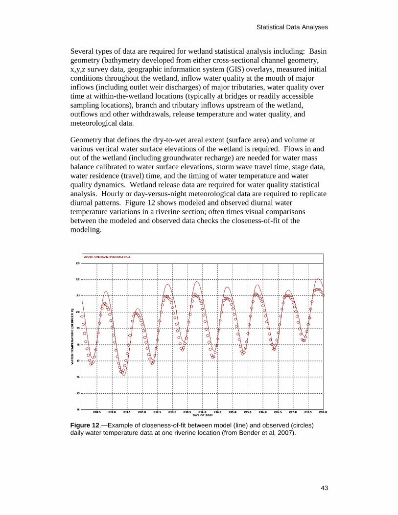
Statistical Data Analyses
43
Several types of data are required for wetland statistical analysis including: Basin geometry (bathymetry developed from either cross-sectional channel geometry, x,y,z survey data, geographic information system (GIS) overlays, measured initial conditions throughout the wetland, inflow water quality at the mouth of major inflows (including outlet weir discharges) of major tributaries, water quality over time at within-the-wetland locations (typically at bridges or readily accessible sampling locations), branch and tributary inflows upstream of the wetland, outflows and other withdrawals, release temperature and water quality, and meteorological data.
Geometry that defines the dry-to-wet areal extent (surface area) and volume at various vertical water surface elevations of the wetland is required. Flows in and out of the wetland (including groundwater recharge) are needed for water mass balance calibrated to water surface elevations, storm wave travel time, stage data, water residence (travel) time, and the timing of water temperature and water quality dynamics. Wetland release data are required for water quality statistical analysis. Hourly or day-versus-night meteorological data are required to replicate diurnal patterns. Figure 12 shows modeled and observed diurnal water temperature variations in a riverine section; often times visual comparisons between the modeled and observed data checks the closeness-of-fit of the modeling.
Figure 12.—Example of closeness-of-fit between model (line) and observed (circles) daily water temperature data at one riverine location (from Bender et al, 2007).
Guidelines for Collecting Data to Support Statistical Analysis of Water Quality for Wetland Planning
44
Water quality data are then added to the statistical analysis to simulate vegetative and algal growth and assimilative capacity of organic matter degradation. A typical case reflecting organic decay is that of a wastewater treatment plant outfall that discharges into a constructed wetland designed to polish the treated wastewater. As water travels through a wetland, oxygen is consumed by decaying nitrogenous and carbonaceous matter resulting in oxygen sag with distance through a fully vegetated wetland. Other constructed wetlands designed for nitrification can have features that aid in aerating water as it moves through the system.
Predicting dynamic wetland characteristics requires an extensive array of equations, coefficients, and measured data that are used to express specific hydraulic transport, heat transfer, and biochemical transformation properties of the wetland. Complete sets of meteorological, water quality, and hydrologic data at the appropriate time intervals are required for all low flow or high flow conditions used for data analysis.
In addition, accurate measurements of physical dimensions, hydraulic structure (weir) configuration, and operations data are required to represent controlling conditions for the wetland. Original design drawings, as-built design drawings, and Project Data (Bureau of Reclamation, hardcopy and 2002 internet link http://www.usbr.gov/projects/) specifications used to provide background for wetland reports should be verified. Historical data compilation and analysis are critical information for wetland design and operation. In 1996, a database of design and operational data from North American treatment wetlands included nitrogen data from 17 constructed surface flow (SF) wetlands, 26 natural SF wetlands, and 9 constructed wetlands (Kadlec and Knight, 1996, page 416). However that database and others have greatly expanded since 1996.
Water mass balance over time is essential to wetland data analysis. For example, “bi-weekly input” data sets are required for the entire period to capture seasonal effects while differentiating changes in dry, average, and wet hydrology or hydraulic fluctuations. Results can often be improved by collecting a broader range of data under dry to wet hydrologic conditions.
Statistical Analysis Techniques SAS, SYSTAT, SPSS, and other computer packages are often used to statistically analyze and plot data. The output from one step typically feeds later steps. For a discussion of statistical analysis techniques commonly used in the statistics packages such as SYSTAT, search the internet.
The output from a spreadsheet or one step of a statistical package may serve as the input to another analysis. The methodology used to statistically analyze data should be documented and included as metadata.
Statistical Data Analyses
45
Representative Flow Conditions and Data Wet, average, median, and dry conditions need to be considered in wetland analysis. Selecting low and wet hydrologic periods to calibrate dry, flood, or spike inflow conditions is a key factor. Wet months with the majority of loading to the wetland tend to occur during the spring of the year. The primary variable for a water mass balance is water surface elevation.
Stage gages that are installed near the wetland outlet control(s) tend to produce better water mass balance results than those derived from inflow gages upstream of the wetland site. If representative data for developing a water mass balance cannot be acquired or estimated, general classifications of hydrologic periods (dry to wet) might be developed based on water surface elevation, precipitation, evaporation, and estimated inflow patterns over long periods of time.
Data Gaps and Model Considerations
Converting data into electronic model input files is the first step in developing an appropriate format for input to empirical models. Identifying and filling in data gaps may be necessary before attempting to develop empirical models.
Role of Statistical Analysis in Wetland Planning and Design
Wetland water quality and empirical modeling capabilities cover a large range of conditions and are developed using measured data that reflect defined (dry-to-wet) dynamic conditions. The empirical model uses these data sets to accurately predict water quality conditions in the wetland environments. Empirical models are used to provide critical planning information for decisions and testing of alternatives before design costs are incurred. If applied properly, empirical models are valuable tools for managing water resources. However, if data supporting the empirical models are lacking, inaccurate information may be produced from the statistical analysis.
Data should be collected to address both parametric and non-parametric statistical methods. Parametric statistics assumes that the data has come from a type of probability distribution and makes inferences about the parameters of the distribution. Parametric statistics tend to be more accurate if assumptions are correct. A normal distribution assumption is one example. Most well-known elementary statistical methods are parametric. However, if the assumptions are incorrect, parametric results can be misleading. Non-parametric methods tend to require a larger sample size to draw conclusions with the same degree of confidence; however, nonparametric methods make fewer assumptions about the data and can be more robust, simpler, and easier to apply. Non-parametric statistics based on the ranks of observations are one example.
Guidelines for Collecting Data to Support Statistical Analysis of Water Quality for Wetland Planning
46
The resulting statistical analysis capabilities provide a long-standing resource that can extend the scope and accuracy of water management investigations. Current state-of-the-art wetland empirical models can accurately represent a range of water quality processes. For example, a statistical analysis and plotting package, such as SYSTAT (SPSS, 2000) could help predict the dynamic effects of operational (flow through) or structural changes (weir height) on water quality or effective duration and degree of influence on wetland vegetation.
Statistical Model Testing
Modeling wetlands is difficult and data intensive. Some attempts have been made to model wetlands (Lee, 1999, Texas A&M and Bureau of Reclamation, 2008). Wetland empirical models should be calibrated and validated with separate data sets. Water travel time determined from continuous Lagragian particle tracking dye studies might be used to test empirical equations. Water quality predictions using empirical models will be more challenging. Due to the large number of variables, expect predictive formulations to apply only part of the time. Comparisons to determine statistically significant differences between conditions are useful; validating the empirical models developed should also be attempted on different wetlands or watersheds.
Other Statistical Model Data Collection Considerations
Empirical model development should consider methods to expand capabilities as additional information is gathered over time. Processing, archival, analysis, presentation of results, and interpretation that support the data quality objectives (DQOs) and quality assurance (QA) plan are required.
QA integrates DQOs, Standardized Operating Procedures (SOPs), and approved methodologies (protocols) with a written description of details. The following QA/QC previously mentioned references have been adopted by Reclamation field personnel:
Bureau of Reclamation, revised August 2003. “Quality Assurance Guidelines for Environmental Measurements.” U.S. Department of the Interior. Originally prepared by QA/QC Implementation Work Group, 1994.
Bureau of Reclamation, September 2003. “Technical Guidelines for Water Quality Investigations. U.S. Department of the Interior.
There are frequent misunderstandings concerning the appropriate application and value of empirical models. Empirical models are statistical, are often tailored to a specific wetland environment, and are developed using actual data and projected operational information.
Data Collection Priorities and Practical Considerations
47
Data Collection Priorities and Practical Considerations Discussions with those who have experience in previous river ecology, monitoring, and modeling studies are helpful in gaining insight into technical issues. Practical experience is important to development of empirical tools for assessing wetlands. As a result, a preliminary assessment is considered a critical step. Data collection and initial assessment development activities for supporting future ecology studies and ongoing planning studies of a wetland can be helpful.
Prioritizing Critical and Secondary Data Sets
Existing data sources should be reviewed to determine common collection sites and problems with proposed sites. Critical and secondary data sets can then be collected and assessed. Increasing levels of data are usually required to increase the certainty of results.
Existing Data Sources and Data Compilation
Initial time spent searching for data and talking to those familiar with historical data collection is time well spent. Most projects have data that go undiscovered.
A program should be put in place to convert data into a modern electronic format. Multiple backups on different types of electronic media are recommended for long-term storage and archival.
Monitoring Plans and Cost Factors
Initially, the project manager should assemble the best possible historical data set, conduct a preliminary data analysis, and then visit the field to survey the site to become familiar with factors affecting the formation and details of the wetland.
Expensive metals analysis and other water quality parameters not modeled with many wetland models should be minimized; however, monitoring data not used in a chosen model may be used in long-term trend analysis. A broad perspective must be considered when laying out a SAP.
Data Review, Analysis, and Processing Concerns
Data collected on the first field trip should be processed, analyzed, and plotted to spot problems or to ensure a complete modeling data set. Adjustments to the SAP may be necessary. Data should also be analyzed and processed in a format that
Guidelines for Collecting Data to Support Statistical Analysis of Water Quality for Wetland Planning
48
optimizes future usability. Developing a method to minimize data processing and time spent on data formatting and analysis is helpful.
Ideally, data should be processed immediately after collection. Analysis of data includes eliminating incorrect data and providing corresponding metadata.
Not developing a protocol introduces error, often results in more wasted efforts as more similar data become available, and results in inconsistencies which make replication of data analysis difficult if the process needs to be repeated.
Conclusions Data analysis can be a useful tool for managing the water quality of a wetland ecosystem. The resulting modeling capabilities are customized to specific characteristics of the wetland system and predefined simulation objectives. Once the complete empirical modeling data collection system is fully operational, the wetland SAP should be assessed for improvements.
Data used outside its intended range can result in misinformation and potentially improper decisions regarding the natural resource and aquatic biota.
Automation of data processing saves time and funding. Assembling multiple data sets at once in an assembly line mode saves time and reduces error.
Guidelines for Collecting Data to Support Statistical Analysis of Water Quality for Wetland Planning
49
References Ambrose, R.B. et al. 1988. “WASP4, A Hydrodynamic and Water Quality
Model—Model Theory, User’s Manual, and Programmer’s Guide,” U.S. Environmental Protection Agency, Athens, GA, EPA/600/3-87-039.
Ambrose, R.B., T.A. Wool, and J.L. Martin, 1993. “The Water Quality Analysis
and Simulation Program, WASP5: Part A, Model Documentation Version 5.1,” U.S. Environmental Protection Agency Athens Environmental Research Laboratory, Athens, Georgia.
American Public Health Association (APHA), American Water Works
Association (AWWA), and Water Environment Federation (WEF), 2005. “Standard Methods for the Examination of Water and Wastewater,” 21st Centennial Edition, Washington, DC.
Atlas, R.M. and Bartha, R., 1987. Microbial Ecology: Fundamentals and
Applications, second edition, The Benjamin/Cummings Publishing Company, Inc., Menlo Park, California.
Bender, M.D., G.E. Hauser, M.C. Shiao, and W.D. Proctor, 1990. “Better: A
Two-Dimensional Reservoir Water Quality Model, Technical Reference Manual and User’s Guide,” Report No. WR28-2-590-152, Tennessee Valley Authority, Engineering Laboratory, Norris, Tennessee.
Bender, Merlynn D., Joseph P. Kubitschek, and Tracy B. Vermeyen, April 2007.
“Temperature Modeling of Folsom Lake, Lake Natoma, and the Lower American River,” U.S. Department of Interior, Bureau of Reclamation, Technical Service Center, Denver, Colorado, Special Report, Prepared for Sacramento Water Forum and the U.S. Fish and Wildlife Service in cooperation with the Mid-Pacific Regional Office, Sacramento, California.
Brown, C. L, and Barnwell, T.O. Jr., 1987. “The enhanced stream water quality
models QUAL2E and QUAL2E-UNCAS documentation and user manual: Athens, Georgia,” U.S. Environmental Protection Agency, Environmental Research Laboratory, EPA/600/3-85-040, 455 p.
Bureau of Reclamation, 1981. “Water and Power Resources Service Project
Data,” A water resources technical publication by the U.S. Department of Interior, Water and Power Resources Service, Denver Colorado, U.S. Government Printing Office.
Bureau of Reclamation, 1981,“Tres Rios Demonstration Constructed Wetlands
Project, Project Status and Water Quality Data Analysis Report. Phase 1 – 1995-1998,” Prepared in cooperation with the City of Phoenix Water
Guidelines for Collecting Data to Support Statistical Analysis of Water Quality for Wetland Planning
50
Services, Available from the National Technical Information Service, Operations Division, 5285 Port Royal Road, Springfield, Virginia 22161 September 2001.
Bureau of Reclamation, 1981,“Survival of Pathogenic Organisms in Constructed
Wetland Systems, Summary Project Report,” Available from the National Technical Information Service, Operations Division, 5285 Port Royal Road, Springfield, Virginia 22161, September 2001.
Bureau of Reclamation, 2002. “Project Data Web,” Public information available
from the U.S. Bureau of Reclamation Internet Web site: http://www.usbr.gov/projects/
Bureau of Reclamation, revised August, 2003. “Quality Assurance Guidelines for
Environmental Measurements,” U.S. Department of the Interior, Originally prepared by QA/QC Implementation Work Group, 1994.
Bureau of Reclamation, September 2003. “Technical Guidelines for Water
Quality Investigations,” U.S. Department of the Interior. Bureau of Reclamation, December 2003,“Cascade Reservoir Created Wetlands
Project, Site Water Quality Monitoring,” prepared in cooperation with the State of Idaho, Department of Environmental Quality.
Bureau of Reclamation, 2008, “Feasibility Design Guidelines, Section 16,
Wetlands,” Public information available from the U.S. Bureau of Reclamation Intranet Web site: http://intra.usbr.gov/~tsc/guidance/design/FDG-Wetlands.pdf or http://www.usbr.gov/pmts/tech_services/engineering/design/data/Chapter3/Chap3_Sec16.pdf
Bureau of Reclamation, May 2009, “Guidelines for Collecting Data to Support
Reservoir Water Quality and Hydrodynamic Simulation models,” U.S. Department of the Interior, Bureau of Reclamation Technical Service Center, Denver, CO, http://www.usbr.gov/pmts/eco_research/hydromodels.pdf.
Bureau of Reclamation, August 2010, “Guidelines for Collecting Data to Support
Riverine Hydrodynamic and Water Quality Simulation Models,” U.S. Department of the Interior, Bureau of Reclamation Technical Service Center, Denver, CO http://www.usbr.gov/pmts/eco_research/river_water_quality_manual.pdf.
Chapra, Steve C. and Pelletier, G.J., November 25, 2003. “QUAL2K: A
Modeling Framework for Simulating River and Stream Water Quality: Documentation and User’s Manual,” Civil and Environmental Engineering Dept., Tufts University, Medford, MA, Steven.Chapra@tufts.
References
51
Cole, T.M., and S.A. Wells, 2002. “CE-QUAL-W2: A Two-Dimensional Laterally Averaged, Hydrodynamic and Water Quality Model, Version 3.1, User Manual.” Draft Instruction Report EL-02-1, Prepared for the U.S. Army Corp of Engineers, Washington, DC.
Cole, T.M., and S.A. Wells, 2006. “CE-QUAL-W2: A Two-Dimensional
Laterally Averaged, Hydrodynamic and Water Quality Model, Version 3.5, User Manual,” Draft Instruction Report EL-06-1, Prepared for the U.S. Army Corp of Engineers, Washington, DC.
Connolly, J.P. and R. Winfield, August 1984. “ A User’s Guide for WASTOX, a
Framework for Modeling the Fate of Toxic Chemicals in Aquatic Environments, Part 1: Exposure Concentration,” U.S. Environmental Protection Agency, Gulf Breeze, Florida, EPA-600/3-84-077.
Connor, Michael L, 2011. “Testimony for FY12 budget request by Michael L.
Connor, Bureau of Reclamation Commissioner,” March 2, 2011 before Natural Resources Committee, Subcommittee on Water and Power, U.S. House of Representatives).
Correll, D.S. and Correll, H.B., 1975. Aquatic and Wetland Plants of
Southwestern United States, Stanford University Press, Stanford, CA, Volumes I and II, ISBN 0-8047-0866-5, 1777 pp.
Cronk, Julie K. and Fennessy, M. Siobhan, 2001. “Wetland Plants, Biology and
Ecology,” CRC Press, Inc., Lewis Publishers, Boca Raton, ISBN 1-56670-372-7, Library of Congress Card Number 2001020390.
Culver, Denise R. and Lemly, Joanna M., 2013. “Field Guide to Colorado’s
Wetland Plants, Identification, Ecology, and Conservation,” Prepared for the U.S. Environmental Protection Agency (EPA) by the Colorado Natural Heritage Program, Warner College of Natural Resources, Colorado State University, Fort Collins, CO, ISBN: 978-0-615-74649-4, printed by Vision Graphics, Inc., Loveland, Colorado.
Daniels, J.S. (Thullen), B.S. Cade, J.J. Sartoris. 2010, “Measuring bulrush culm
relationships to estimate plant biomass within a southern California constructed wastewater surface-flow wetland,” Wetlands 30(2): 231-239.
Daniels, J.S., May 5, 2013 personal communication. Di Toro, D.M., J.J. Fitzpatrick, and R.V. Thomann, 1981, rev. 1983. “Water
Quality Analysis Simulation Program (WASP) and Model Verification Program (MVP) – Documentation,” Hydroscience, Inc., Westwood, NY, for U.S. EPA, Duluth, MN, Contract No. 68-01-3872.
Guidelines for Collecting Data to Support Statistical Analysis of Water Quality for Wetland Planning
52
Environmental Protection Agency, September, 1988. “Design Manual: Constructed Wetlands and Aquatic Plant Systems for Municipal Wastewater Treatment,” EPA/625/1-88/022, Office of Research and Development, Cincinnati, OH. http://water.epa.gov/type/wetlands/upload/design.pdf
Environmental Protection Agency, 1993. “Created and Natural Wetlands for
Controlling Nonpoint Source Pollution,” Edited by Richard K. Olsen, Office of Research and Development and Office of Wetlands, Oceans, and Watersheds, C. K. Smoley, CRC Press, Inc., Boca Raton, Florida
Environmental Protection Agency, 1993. “Subsurface Flow Constructed Wetlands
for Wastewater Treatment: A Technology Assessment (1993) (Office of Wastewater Management, Washington, DC, EPA 832-R-93-008).
Environmental Protection Agency, 1993. “Habitat Quality Assessment of Wetland
Treatment Systems,” (3 studies in 1992 and 1993) (Environmental Research Lab, Corvallis, OR, EPA 600-R-92-229, EPA 600-R-93-117, EPA 600-R-93-222).
Environmental Protection Agency, 1993. “Wildlife Habitat: 17 Case Studies,”
Office of Wastewater Management, Washington, DC, EPA 832-R-93-005. Environmental Protection Agency, 1995. “Guidance for Design and Construction
of a Subsurface Flow Constructed Wetland (August 1993) (USEPA Region VI, Municipal Facilities Branch).
Environmental Protection Agency, 1995. “Handbook of Constructed Wetlands,”
5 volumes, USEPA Region III with USDA, NRCS, ISBN 0-16-052999-9. Environmental Protection Agency, 1997. “Constructed Wetlands for Animal
Waste Treatment: A Manual on Performance, Design, and Operation With Cases Histories,” USEPA Gulf of Mexico Program.
Environmental Protection Agency, 1999. “Free Water Surface Wetlands for
Wastewater Treatment: A Technology Assessment (1999) (Office of Wastewater Management, Washington, DC, EPA /832/R-99/002).
Environmental Protection Agency, 1993 “Constructed Wetlands: Treatment of
Municipal Wastewaters,” Office of Research and Development Cincinnati, OH, (EPA/625/R-99/010), http://water.epa.gov/type/wetlands/restore/upload/constructed-wetlands-design-manual.pdf
Environmental Protection Agency, September, 2000. “Manual: Constructed
Wetlands Treatment of Municipal Wastewaters,” Office of Research and Development, Cincinnati, OH, EPA 625-R-99-010, https://ceprofs.civil.tamu.edu/.../15.%20EPA%20Constructed%20Wetlands.pdf
References
53
Environmental Protection Agency, October 2000. “Guiding Principles for Constructed Treatment Wetlands: Providing for Water Quality and Wildlife Habitat”, developed by The Interagency Workgroup on Constructed Wetlands, U.S. EPA, U.S. Army Corps of Engineers, U.S. Fish & Wildlife Service, Natural Resources Conservation Service, National Marine Fisheries Service, U.S. Bureau of Reclamation, EPA 843-B-00-003.
Ferrari, R.L., and K. Collins, 2006. “Reservoir Survey and Data Analysis,”
Chapter 9, Erosion and Sedimentation Manual, Bureau of Reclamation, Sedimentation and River Hydraulics Group, Denver, Colorado, http://www.usbr.gov/pmts/sediment.
Hammer, Donald A., 1992. “Creating Freshwater Wetlands,” CRC Press, Inc.,
Lewis Publishers, Boca Raton, ISBN 0-87371-445-8. Hamrick, J. M. 1996. “A User’s Manual for the Environmental Fluid Dynamics
Computer Code (EFDC),” Special Report 331, The College of William and Mary, Virginia Institute of Marine Science, Gloucester Point, VA.
Hauser, G.E. and G. A. Schohl, November 2002. “River Modeling System v4 –
User Guide and Technical Reference,” Report No. WR28-1-590-164, TVA River System Operations and Environment, Norris, Tennessee, (Revised June, 2003 in draft).
Hunt, Brandy, 2002. “Determining the Actual Hydraulic Retention Time of a
Constructed Wetland Cell for Comparison With the Theoretical Hydraulic Retention Time,” Master of Science Thesis submitted to the University of Georgia, Athens, Georgia. Pdf available online via google search
Kadlec, Robert H. and Knight, Robert L., 1996, “Treatment Wetlands,” CRC
Press, Inc., Lewis Publishers, Boca Raton, ISBN 0-87371-930-1, Library of Congress Card Number 95-9492, 893 pp.
Kadlec, R.H., Wallace, S. D. 2009, “Treatment Wetlands: Second Edition,”
CRC/Lewis Publishers, Taylor and Francis Group, Boca Raton, FL, ISBN 978-1-56670-526-4, 1016 pp.
Keefe, Steffanie H., Joan S. (Thullen) Daniels, Robert L. Runkel, Roland D. Wass, Eric A. Stiles, and Larry B. Barber, 2010, “Influence of hummocks and emergent vegetation on hydraulic performance in a surface flow wastewater treatment wetland. Water Resources Research, 46, W11518, doi:10.1029/2010WR009512, 13 pp.
Lee, Erik Ryan, 1999. “Set-Wet: A Wetland Simulation Model to Optimize
Nonpoint Source Pollution Control,” Master of Science Thesis submitted to the Virginia Polytechnic Institute and the Virginia State University,
Guidelines for Collecting Data to Support Statistical Analysis of Water Quality for Wetland Planning
54
Blacksburg Virginia. scholar.lib.vt.edu/theses/available/etd.../ERIKLEE1ETD.PDF
Martin, James L. and Tim A. Wool, 2002. “Dynamic one dimensional model of
hydrodynamics and water quality EPD-RIV1, “Version 1.0, User’s Manual, AScI Cooperation, Athens, Georgia, (http://www.epdsoftware.com/Download/EpdRiv1.pdf).
Mitsch, W.J., Gosselink, J.G., 2000, “Wetlands,” Third Edition, John Wiley &
Sons, Inc., New York, NY, 920 pp. Moshiri, Gerald A., 1993, “Constructed Wetlands for Water Quality
Improvement,” CRC Press, Inc., Lewis Publishers, Boca Raton, ISBN 0-87371-550-0, Library of Congress Card Number 92-46759
Mulamoottil, George, Warner, Barry G., and McBean, Edward A., 1996,
“Wetlands, Environmental Gradients, Boundaries, and Buffers,” CRC Press, Inc., Boca Raton, Florida
Novotny, Vladimir, Ehsan Kianirad, David Dedoya, Indrani Ghosh, and Devin
McGarvey, 2006, “ Review of Watershed Ecological Models,” Technical Report No. 7, Center for Urban Environmental Studies, northeastern University, Boston, Massachusetts (http://www.coe.neu.edu/.../TR-7-Review%20of%20Watershed%20Ecological%20models.pdf).
Orange County Water District, 2006, “Dairy Washwater Treatment Wetlands
Demonstration Project,” O’connor, Katherine A., A.I.C.P., Lyon, Stephen, Phd. Orange County Water District, Fountain Valley, CA.
Park, R. A., and J. S. Clough. 2004, “Aquatox (Release 2): Modeling
Environmental Fate and Ecological Effects in Aquatic Ecosystems, Volume 2: Technical Documentation,” U.S. Environmental Protection Agency, Office of Water, Washington, DC.
Sartoris, J.J., J.S. Thullen, and L.B. Barber, 2000a, “Effect of hemi-marsh
reconfiguration on nitrogen transformations in a southern California treatment wetland.” In: 7th International Conference on Wetland Systems for Water Pollution Control, November 11-16, 2000, Lake Buena Vista, Florida, Volume I, London: IWA Pub. p. 359-364.
Sartoris, J.J., J.S. Thullen, L.B. Barber, and D.E. Salas, 2000b, “Investigation of
nitrogen transformations in a southern California constructed wastewater treatment wetland.” Ecological Engineering 14(1-2): 49-65.
Smith, R. Daniel, Alan Amman, Candy Bortoldus, and Mark M. Brinson. October
1995. “An Approach for Assessing Wetland Functions Using
References
55
Hydrogeomorphic Classification, Reference Wetlands, and Functional Indices,” U.S. Army Corp of Engineers, Waterways Experiment Station (WES), Wetlands Research Program technical report, series TA7 W34 no. WRP-DE-9.
SPSS, 2000, “SYSTAT User’s Manual,” version 10, SYSTAT Statistical analysis
software user’s manual and documentation, SPSS, Inc., Chicago, Illinois, SYSTAThttp://www.molar.unibe.ch/help/statistics/systat/statistics.pdf.
Texas A&M and Bureau of Reclamation, 2008. “2008 Modeling Inventory,”
U.S. Department of the Interior, Bureau of Reclamation, Denver Technical Service Center, Denver, CO.
Thullen, J.S., J.J. Sartoris, and W.E. Walton, 2002, “Effects of vegetation
management in constructed wetland treatment cells on water quality and mosquito production,” Ecological Engineering 18: 441-457.
Thullen, J.S., J.J. Sartoris, and S.M. Nelson, 2005, “Managing vegetation in
surface-flow wastewater-treatment wetlands for optimal treatment performance,” Ecological Engineering 25: 583-593.
Thullen, J.S., S.M. Nelson, B.S. Cade, J.J. Sartoris, 2008, “Macrophyte
decomposition in a surface-flow constructed wetland: rates associated with environmental and biotic variables,” Ecological Engineering 32:281-290.
United States Army Corp of Engineers (USACE), Environmental Laboratory,
1982. “CE-QUAL-R1: A Numerical One-Dimensional Model of Reservoir Water-Quality; User’s Manual,” Instruction Report E-82-1 (Revised Edition supersedes IR E-82-1, dated April 1982), U.S. Army Engineer Waterways Experiment Station, Vicksburg, Mississippi.
United States Army Corp of Engineers (USACE), Environmental Laboratory,
January 1987, “Corps of Engineers Wetlands Delineation Manual,” Final Technical Report Y-87-1 USACE Waterways Experiment Station, Vicksburg, MS http://el.erdc.usace.army.mil/wetlands/pdfs/wlman87.pdf
United States Army Corp of Engineers (USACE), April 2008. “The Interim
Regional Supplement to the Corps of Engineers Wetland Delineation Manual: Western Mountains, Valleys, and Coast Regions,” Final Report No. ERDC/EL TR-08-13, Environmental Laboratory, USACE Environmental Research and Development Center, Vicksburg, MS. http://www.usace.army.mil/CECW/Documents/cecwo/reg/west_mt_finalsupp.pdf For a list of additional regional supplements: http://www.usace.army.mil/cecw/pages/reg_supp.aspx

Guidelines for Collecting Data to Support Statistical Analysis of Water Quality for Wetland Planning
56
Wetzel, R.G., 2001, Limnology: Lake and River Ecosystems, 3rd. Edition, Academic Press, New York, NY, ISBN: 0127447601.
Wool, Tim A., Ambrose, Robert B., Martin, James L., Comer, Edward A., “Water
Quality Analysis Simulation Program (WASP) Version 6.0 Draft: User’s Manual,” U.S. Environmental Protection Agency, Athens, GA, http://chiwater.com/Company/Staff/WJamesWebpage/original/homepage/Teaching/661/WASP6_Manual.pdf
Appendix A Wetland Data Collection and Statistical Analysis Examples and Modeling Approaches

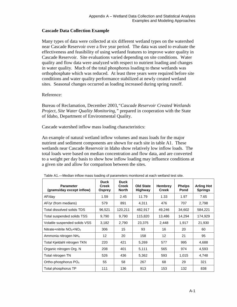
Appendix A – Wetland Data Collection and Statistical Analysis Examples and Modeling Approaches
A-1
Cascade Data Collection Example Many types of data were collected at six different wetland types on the watershed near Cascade Reservoir over a five year period. The data was used to evaluate the effectiveness and feasibility of using wetland features to improve water quality in Cascade Reservoir. Site evaluations varied depending on site conditions. Water quality and flow data were analyzed with respect to nutrient loading and changes in water quality. Much of the total phosphorus loading to these wetlands was orthophosphate which was reduced. At least three years were required before site conditions and water quality performance stabilized at newly created wetland sites. Seasonal changes occurred as loading increased during spring runoff. Reference: Bureau of Reclamation, December 2003,“Cascade Reservoir Created Wetlands Project, Site Water Quality Monitoring,” prepared in cooperation with the State of Idaho, Department of Environmental Quality. Cascade watershed inflow mass loading characteristics: An example of natural wetland inflow volumes and mass loads for the major nutrient and sediment components are shown for each site in table A1. These wetlands near Cascade Reservoir in Idaho show relatively low inflow loads. The total loads were based on median concentration and flow data, and are converted to a weight per day basis to show how inflow loading may influence conditions at a given site and allow for comparison between the sites.
Table A1.—Median inflow mass loading of parameters monitored at each wetland test site.
Parameter (grams/day except inflow)
Duck Creek
Osprey
Duck Creek North
Old State Highway
Hembrey Creek
Phelps Pond
Arling Hot Springs
AF/day 1.59 2.45 11.79 1.33 1.97 7.65
AF/yr (from medians) 579 891 4,311 476 707 2,798
Total dissolved solids TDS 96,521 120,211 482,917 49,246 34,602 584,221
Total suspended solids TSS 9,790 9,790 115,820 13,486 14,294 174,929
Volatile suspended solids VSS 3,182 2,790 23,375 2,448 1,917 21,930
Nitrate+nitrite NO3+NO2 306 15 93 16 20 60
Ammonia nitrogen NH4 12 20 158 12 21 95
Total Kjeldahl nitrogen TKN 220 421 5,269 577 995 4,688
Organic nitrogen Org. N 208 401 5,111 565 974 4,593
Total nitrogen TN 526 436 5,362 593 1,015 4,748
Ortho-phosphorus PO4 55 58 267 68 29 321
Total phosphorus TP 111 136 913 153 132 838
Guidelines for Collecting Data to Support Statistical Analysis of Water Quality for Wetland Planning
A-2
Tres Rios Groundwater Recharge and Reuse Example The Tres Rios Demonstration Constructed Wetland Project provides a foundation to evaluate technical, practical, and institutional factors involved to incorporate constructed wetlands in comprehensive water management plans. It reflects widespread interest in pursuing more effective, integrated approaches to sustain valuable water and environmental resources in arid regions of the western United States. When considered collectively, the demonstration monitoring program and parallel activities have provided a wealth of information to advance constructed wetlands technology and insight into practical and institutional considerations to effectively incorporate wetlands in water resource planning. This report summarizes project activities and water quality characteristics of the demonstration wetlands based on the first phase of monitoring from 1995 through 1998. Water quality results and findings are interpreted with respect to the demonstration objectives, the status of constructed wetlands technology, and implications for future water resource planning. Many conclusions were drawn from the Tres Rios study. Of particular interest was the net removal for all monitored constituents even at very low concentration levels, the significant effects of hydraulic operations including depths and flow rates, and the transient shifts in temperature, oxygen, and related transformation properties that may indicate the balance between external and internal loading and the net effects of assimilation processes. Wetland configuration effects were relatively subtle in comparison to the changes evident under different operating conditions. Removal efficiencies for BOD, TSS, and TN tended to be less than reported from the literature (City of Phoenix, September 2001, Table 5-2). Reference:
Bureau of Reclamation, September 2001, “Tres Rios Demonstration Constructed Wetlands Project, Project Status and Water Quality Data Analysis Report. Phase 1 – 1995-1998,” Prepared in cooperation with the City of Phoenix Water Services, Available from the National Technical Information Service, Operations Division, 5285 Port Royal Road, Springfield, Virginia 22161.
Appendix A – Wetland Data Collection and Statistical Analysis Examples and Modeling Approaches
A-3
Example of Data Collection for Pathogenic Organisms Pathogenic organisms and enteric viruses are significant public health concerns worldwide. Although the transport, exposure, and persistence of pathogens have been studied extensively in receiving streams, less is known about their behavior in wetland systems constructed to further polish treated wastewater. This investigation examined hydraulic transport and survival characteristics of the pathogenic viruses through laboratory microcosm experiments and field studies using a non-pathogenic MS2 coliphage surrogate and selected water analyses to isolate and quantify actual virus pathogens from a test constructed wetlands system. This study showed that wetlands could be used to remove the majority of pathogenic organisms; however, the removal rate did not satisfy the removal for drinking water treatment. Reference: Bureau of Reclamation, September 2001,“Survival of Pathogenic Organisms in Constructed Wetland Systems, Summary Project Report,” Available from the National Technical Information Service, Operations Division, 5285 Port Royal Road, Springfield, Virginia 22161.

Guidelines for Collecting Data to Support Statistical Analysis of Water Quality for Wetland Planning
A-4
Another Approach is to use Mathematical Models WASP, EPD-RIV1, AQUATOX, QUAL2E (Brown and Barnwell, 1987), QUAL2K (Chapra et al., 2003), CEQUALW2 (Cole and Wells, 2002 and 2006), SPAW, POND, and others have been used on wetlands. Modeling wetlands is a challenge that often results in custom building a tool for a particular wetland. One-dimensional backwater models (Hauser and Schohl, 2002 and USACE, 1982) might be attempted on deep wetlands if sufficient flow through the wetland exists. Watershed ecological models might also be attempted (Novotny el al., 2006). A review of available models has been done by Texas A&M and Bureau of Reclamation (2008). Application of mathematical models to wetlands requires extensive resources, expertise, and time to develop. For example, three manuals are included with SPAW model distribution. An “Operational Manual” assists with run-time questions, a “User’s Manual” is an introduction to the SPAW model and its typical applications, and a “Reference Manual” includes details about the internal model methods, assumptions and calculations. Therefore statistical analysis of wetlands is preferred to model development.
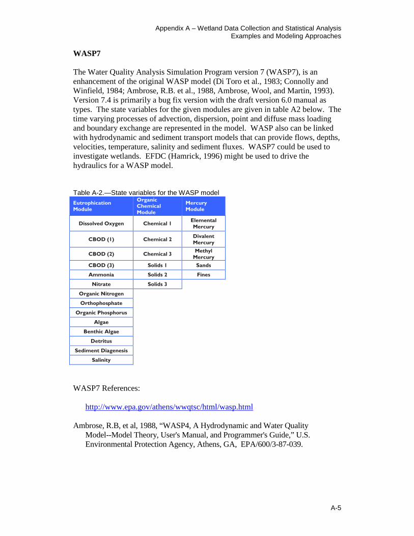
Appendix A – Wetland Data Collection and Statistical Analysis Examples and Modeling Approaches
A-5
WASP7 The Water Quality Analysis Simulation Program version 7 (WASP7), is an enhancement of the original WASP model (Di Toro et al., 1983; Connolly and Winfield, 1984; Ambrose, R.B. et al., 1988, Ambrose, Wool, and Martin, 1993). Version 7.4 is primarily a bug fix version with the draft version 6.0 manual as types. The state variables for the given modules are given in table A2 below. The time varying processes of advection, dispersion, point and diffuse mass loading and boundary exchange are represented in the model. WASP also can be linked with hydrodynamic and sediment transport models that can provide flows, depths, velocities, temperature, salinity and sediment fluxes. WASP7 could be used to investigate wetlands. EFDC (Hamrick, 1996) might be used to drive the hydraulics for a WASP model. Table A-2.—State variables for the WASP model Eutrophication Module
Organic Chemical Module
Mercury Module
Dissolved Oxygen Chemical 1 Elemental Mercury
CBOD (1) Chemical 2 Divalent Mercury
CBOD (2) Chemical 3 Methyl
Mercury
CBOD (3) Solids 1 Sands
Ammonia Solids 2 Fines
Nitrate Solids 3
Organic Nitrogen
Orthophosphate
Organic Phosphorus
Algae
Benthic Algae
Detritus
Sediment Diagenesis
Salinity
WASP7 References:
http://www.epa.gov/athens/wwqtsc/html/wasp.html
Ambrose, R.B, et al, 1988, “WASP4, A Hydrodynamic and Water Quality Model--Model Theory, User's Manual, and Programmer's Guide,” U.S. Environmental Protection Agency, Athens, GA, EPA/600/3-87-039.
Guidelines for Collecting Data to Support Statistical Analysis of Water Quality for Wetland Planning
A-6
Ambrose, R.B., T.A. Wool, and J.L. Martin. 1993, “The Water Quality Analysis and Simulation Program, WASP5: Part A, Model Documentation Version 5.1,” U. S. Environmental Protection Agency, Athens Environmental Research Laboratory, Athens, Georgia.
WASP version 7.41 webpage: http://www.epa.gov/athens/wwqtsc/html/wasp.html Wool, Tim A., Ambrose, Robert B., Martin, James L., Comer, Edward A., “Water
Quality Analysis Simulation Program (WASP) Version 6.0 Draft: User’s Manual,” U.S. Environmental Protection Agency, Athens, GA, http://chiwater.com/Company/Staff/WJamesWebpage/original/homepage/Teaching/661/WASP6_Manual.pdf
Other models have also been used for wetlands. Martin, James L. and Tim A. Wool, 2002, “Dynamic one dimensional model of
hydrodynamics and water quality EPD-RIV1, “Version 1.0, User’s Manual, AScI Cooperation, Athens, Georgia. (http://www.epdsoftware.com/Download/EpdRiv1.pdf)
Park, R. A., and J. S. Clough. 2004, “Aquatox (Release 2): Modeling
Environmental Fate and Ecological Effects in Aquatic Ecosystems, Volume 2: Technical Documentation,” U.S. Environmental Protection Agency, Office of Water, Washington, DC.
Brown, C. L, and Barnwell, T.O. Jr., 1987, “The enhanced stream water quality
models QUAL2E and QUAL2E-UNCAS documentation and user manual: Athens, Georgia,” U.S. Environmental Protection Agency, Environmental Research Laboratory, EPA/600/3-85-040, 455 p.
Chapra, Steve C. and Pelletier, G.J., November 25, 2003, “QUAL2K: A
Modeling Framework for Simulating River and Stream Water Quality: Documentation and User’s Manual,” Civil and Environmental Engineering Dept., Tufts University, Medford, MA, Steven.Chapra@tufts.
Appendix B Statistical Data Analysis Methods


Appendix B – Statistical Data Analysis Methods
B-1
The following pages (reproduced from Bureau of Reclamation, December 2003, “Cascade Reservoir Created Wetlands Project, Site Water Quality Monitoring”) include basic descriptions for statistical analysis methods excerpted from the SYSTAT software help menus. Further information is available in the complete SYSTAT documentation and product support found online (SPSS, 1998 and more recent information).

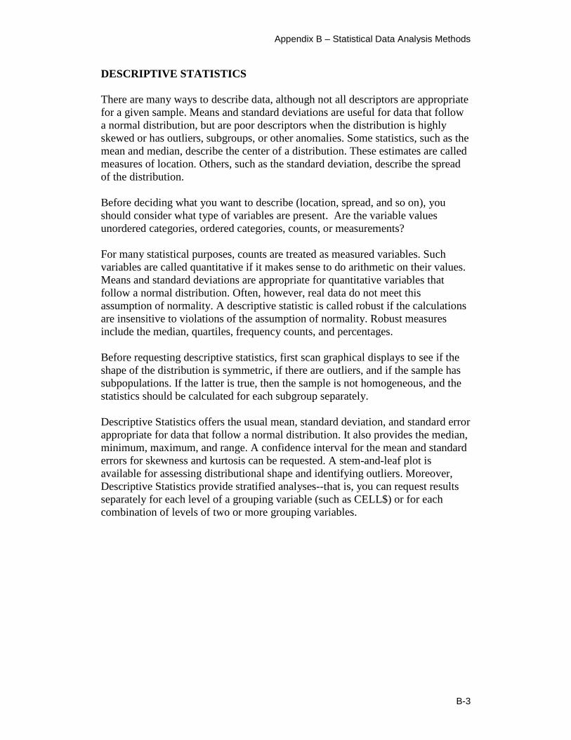
Appendix B – Statistical Data Analysis Methods
B-3
DESCRIPTIVE STATISTICS There are many ways to describe data, although not all descriptors are appropriate for a given sample. Means and standard deviations are useful for data that follow a normal distribution, but are poor descriptors when the distribution is highly skewed or has outliers, subgroups, or other anomalies. Some statistics, such as the mean and median, describe the center of a distribution. These estimates are called measures of location. Others, such as the standard deviation, describe the spread of the distribution. Before deciding what you want to describe (location, spread, and so on), you should consider what type of variables are present. Are the variable values unordered categories, ordered categories, counts, or measurements? For many statistical purposes, counts are treated as measured variables. Such variables are called quantitative if it makes sense to do arithmetic on their values. Means and standard deviations are appropriate for quantitative variables that follow a normal distribution. Often, however, real data do not meet this assumption of normality. A descriptive statistic is called robust if the calculations are insensitive to violations of the assumption of normality. Robust measures include the median, quartiles, frequency counts, and percentages. Before requesting descriptive statistics, first scan graphical displays to see if the shape of the distribution is symmetric, if there are outliers, and if the sample has subpopulations. If the latter is true, then the sample is not homogeneous, and the statistics should be calculated for each subgroup separately. Descriptive Statistics offers the usual mean, standard deviation, and standard error appropriate for data that follow a normal distribution. It also provides the median, minimum, maximum, and range. A confidence interval for the mean and standard errors for skewness and kurtosis can be requested. A stem-and-leaf plot is available for assessing distributional shape and identifying outliers. Moreover, Descriptive Statistics provide stratified analyses--that is, you can request results separately for each level of a grouping variable (such as CELL$) or for each combination of levels of two or more grouping variables.
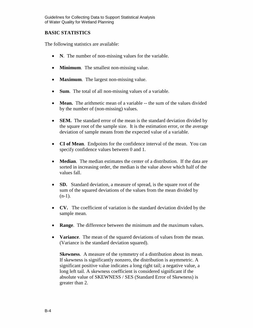
Guidelines for Collecting Data to Support Statistical Analysis of Water Quality for Wetland Planning
B-4
BASIC STATISTICS The following statistics are available:
• N. The number of non-missing values for the variable.
• Minimum. The smallest non-missing value.
• Maximum. The largest non-missing value.
• Sum. The total of all non-missing values of a variable.
• Mean. The arithmetic mean of a variable -- the sum of the values divided by the number of (non-missing) values.
• SEM. The standard error of the mean is the standard deviation divided by the square root of the sample size. It is the estimation error, or the average deviation of sample means from the expected value of a variable.
• CI of Mean. Endpoints for the confidence interval of the mean. You can specify confidence values between 0 and 1.
• Median. The median estimates the center of a distribution. If the data are sorted in increasing order, the median is the value above which half of the values fall.
• SD. Standard deviation, a measure of spread, is the square root of the sum of the squared deviations of the values from the mean divided by (n-1).
• CV. The coefficient of variation is the standard deviation divided by the sample mean.
• Range. The difference between the minimum and the maximum values.
• Variance. The mean of the squared deviations of values from the mean. (Variance is the standard deviation squared). Skewness. A measure of the symmetry of a distribution about its mean. If skewness is significantly nonzero, the distribution is asymmetric. A significant positive value indicates a long right tail; a negative value, a long left tail. A skewness coefficient is considered significant if the absolute value of SKEWNESS / SES (Standard Error of Skewness) is greater than 2.

Appendix B – Statistical Data Analysis Methods
B-5
• Kurtosis. A value of kurtosis significantly greater than 0 indicates that the variable has longer tails than those for a normal distribution; less than 0 indicates that the distribution is flatter than a normal distribution. A kurtosis coefficient is considered significant if the absolute value of KURTOSIS / SEK (Standard Error of Kurtosis) is greater than 2.
• Confidence. Confidence level for the confidence interval of the mean. Enter a value between 0 and 1. (0.95 and 0.99 are typical values).
Guidelines for Collecting Data to Support Statistical Analysis of Water Quality for Wetland Planning
B-6
LINEAR MODELS I: LINEAR REGRESSION The model for simple linear regression is:
y = β0 + β1x + ε where y is the dependent variable, x is the independent variable, and the β’s are the regression parameters (the intercept and the slope of the line of best fit). The model for multiple linear regression is:
y = β0 + β1x1 + β2 x2 +…+ βpxp + ε Both Regression and General Linear Model (GLM) can estimate and test simple and multiple linear regression models. Regression is easier to use than General Linear Model when you are doing simple regression, multiple regression, or stepwise regression because it has fewer options. To include interaction terms in your model or for mixture models, use General Linear Model. With Regression, all independent variables must be continuous; in General Linear Model, you can identify categorical independent variables and SYSTAT will generate a set of design variables for each. Both General Linear Model and Regression allow you to save residuals. In addition, you can test a variety of hypotheses concerning the regression coefficients using General Linear Model. The ability to do stepwise regression is available in three ways: use the default values, specify your own selection criteria, or at each step, interactively select a variable to add or remove from the model. For each model you fit in REGRESS, SESTET reports R2, adjusted R2, the standard error of the estimate, and an ANOVA table for assessing the fit of the model. For each variable in the model, the output includes the estimate of the regression coefficient, the standard error of the coefficient, the standardized coefficient, tolerance, and a t statistic for measuring the usefulness of the variable in the model.
Appendix B – Statistical Data Analysis Methods
B-7
T TEST T TEST provides three types of tests:
• The two-sample t test (independent t test) to compare the mean of one variable for two groups of cases.
• The paired comparison t test (dependent t test) to compare the means of two variables for a single group. The matched pairs t test is a variation of the paired t test.
• The one-sample t test to compare the mean of one variable with a known or hypothesized value.
T Tests [description] The following t tests are available on the Statistics menu: Two Groups Two-sample (independent) t test. The values of the variable of
interest (for example, INCOME) are stored in a single column and SYSTAT uses codes of a grouping variable (for example, GENDER) to separate the cases into two groups (the codes can be numbers or characters). SYSTAT tests whether the difference between the two means differs from 0.
Paired Paired comparison (dependent) t test. For each case used in a paired t
test, SYSTAT computes the differences between values of two variables (columns) and tests whether the average differs from 0.
One-Sample One-sample t test. For the one-sample t test, values of a single
variable are compared against a constant that you specify. WILCOXON SIGNED-RANK TEST The Wilcoxon test compares the rank values of the variables you select, pair by pair, and displays the count of positive and negative differences. For ties, the average rank is assigned. It then computes the sum of ranks associated with positive differences and the sum of ranks associated with negative differences. The test statistic is the lesser of the two sums of ranks.
Guidelines for Collecting Data to Support Statistical Analysis of Water Quality for Wetland Planning
B-8
KRUSKAL-WALLIS [ONEWAY ANOVA TEST] For the Kruskal-Wallis test, the values of a variable are transformed to ranks (ignoring group membership) to test that there is no shift in the center of the groups (that is, the centers do not differ). This is the nonparametric analog of a one-way analysis of variance. When there are only two groups, this procedure reduces to the Mann-Whitney test, the nonparametric analog of the two-sample t test. Variables(s): SYSTAT computes a separate test for each variable in the Variable(s) list. Grouping Variable. The grouping variable can be string or numeric.
Appendix B – Statistical Data Analysis Methods
B-9
LINEAR MODELS II: ANALYSIS OF VARIANCE SYSTAT handles a wide variety of balanced and unbalanced analysis of variance designs. The Analysis of Variance (ANOVA) procedure includes all interactions in the model and tests them automatically; it also provides analysis of covariance, and repeated measures designs. After you have estimated your ANOVA model, it is easy to test post hoc pairwise differences in means or to test any contrast across cell means, including simple effects. For models with fixed and random effects, you can define error terms for specific hypotheses. You can also do stepwise ANOVA (that is, Type I sums of squares). Categorical variables are entered or deleted in blocks, and you can examine interactively or automatically all combinations of interactions and main effects. The General Linear Model (GLM) procedure is used for randomized block designs, incomplete block designs, fractional factorials, Latin square designs, and analysis of covariance with one or more covariates. GLM also includes repeated measures, split plot, and crossover designs. It includes both univariate and multivariate approaches to repeated measures designs. Moreover, GLM also features the means model for missing cells designs. Furthermore, the means model allows direct tests of simple hypotheses (for example, within levels of other factors). Finally, the means model allows easier use of population weights to reflect differences in subclass sizes. For both ANOVA and GLM, group sizes can be unequal for combinations of grouping factors; but for repeated measures designs, each subject must have complete data. You can use numeric or character values to code grouping variables. You can store results of the analysis (predicted values and residuals) for further study and graphical display. In ANCOVA (using COVARIATE), you can save adjusted cell means. ANOVA: Analysis of Variance SYSTAT provides two procedures for analysis of variance: Analysis of Variance (ANOVA) and General Linear Model (GLM). ANOVA is easier to use, because it includes all interactions in the model and tests them automatically. You can specify covariates, do repeated measures, save residuals, and test post hoc pairwise differences in means. Group sizes can be unequal for combinations of grouping factors, but each subject must have complete data across repeated measures. You can use numeric or character values to code grouping variables. You can store results of the analysis (predicted values and residuals) for further study and graphical display. In ANCOVA (using COVARIATE), you can save adjusted cell means.
Guidelines for Collecting Data to Support Statistical Analysis of Water Quality for Wetland Planning
B-10
CORRELATIONS Variables. Available only if One is selected for Sets. All selected variables are correlated with all other variables in the list, producing a triangular correlation matrix. Rows. Available only if Two is selected for Sets. Selected variables are correlated with all column variables, producing a rectangular matrix. Columns. Available only if Two is selected for Sets. Selected variables are correlated with all row variables, producing a rectangular matrix. Sets. One set creates a single, triangular correlation matrix of all variables in the Variable(s) list. Two sets create a rectangular matrix of variables in the Row(s) list correlated with variables in the Column(s) list. Listwise. Listwise deletion of missing data. Any case with missing data for any variable in the list is excluded. Pairwise. Pairwise deletion of missing data. Only cases with missing data for one of the variables in the pair being correlated are excluded. Save file. Saves the correlation matrix to a file. Types. Type of data or measure. You can select from a variety of distance measures, as well as measures for continuous data (e.g. Pearson), rank-order data (e.g. Spearman), and binary data. MEASURES FOR RANK-ORDER DATA If your data are simply ranks of attributes, or if you want to see how well variables are associated when you pay attention to rank ordering, you should consider the following measures available for ranked data:
• Spearman. Produces a matrix of Spearman rank-order correlation coefficients. This measure is a nonparametric version of the Pearson correlation coefficient, based on the ranks of the data rather than the actual values.

Appendix B – Statistical Data Analysis Methods
B-11
MEASURES FOR CONTINUOUS DATA The following measures are available for continuous data: Pearson. Produces a matrix of Pearson product-moment correlation coefficients. Pearson correlations vary between -1 and +1. A value of 0 indicates that neither of two variables can be predicted from the other by using a linear equation. A Pearson correlation of 1 or -1 indicates that one variable can be predicted perfectly by a linear function of the other.
Filename: C:\1wordDP\wetlandWP2012\Wetland water quality manual32.docx


![Statistical guidelines for sampling marine avian populations... · Statistical Guidelines for sampling marine avian populations Zipkin_IWMC_2012_Session 30.ppt [Compatibility Mode]](https://img.pdfslide.net/doc/110x75/612d84491ecc515869423d16/statistical-guidelines-for-sampling-marine-avian-populations-statistical-guidelines.jpg)