Hamiltonian Dynamics Sampling

Abstract

Hamiltonian Dynamics Monte Carlo is a popular method used in simulating complicated distribution.The performance of HMC highly depends on geometry of the momentum-state dual space; we investigateseveral pathological dual space that leads to the failure of HMC from high level geometric perspective. Thisincludes isolated modes, high curvature and multiple spatial scales occurs in dual space. We summariesseveral approaches that improve the results. We reinterpret the Riemannian Manifold HMC from theperspective of the relationship between Hessian and Co-variance as this can better explain the frame topropose a General Riemannian Metrics for a better generalization of Manifold HMC. We also adapt thestepsize and leapfrog steps of continuously tempered HMC to improve the performance and generate alarger number of effective samples.

Contents

1 Introduction1.1 Motivation . . . . . . . . . . . . . . . . . . . . . . . . . . . . . . . . . . . . . . . . . . . . . . . .1.2 Basics . . . . . . . . . . . . . . . . . . . . . . . . . . . . . . . . . . . . . . . . . . . . . . . . . . .1.3 Challenges . . . . . . . . . . . . . . . . . . . . . . . . . . . . . . . . . . . . . . . . . . . . . . . .1.4 Monte Carlo Method . . . . . . . . . . . . . . . . . . . . . . . . . . . . . . . . . . . . . . . . . .

2 Hamiltonian Monte Carlo2.1 Motivation . . . . . . . . . . . . . . . . . . . . . . . . . . . . . . . . . . . . . . . . . . . . . . . .2.2 Typical Set . . . . . . . . . . . . . . . . . . . . . . . . . . . . . . . . . . . . . . . . . . . . . . . .2.3 Hamiltonian Dynamics . . . . . . . . . . . . . . . . . . . . . . . . . . . . . . . . . . . . . . . . .

2.3.1 Analogous . . . . . . . . . . . . . . . . . . . . . . . . . . . . . . . . . . . . . . . . . . . .2.3.2 Condition for HMC . . . . . . . . . . . . . . . . . . . . . . . . . . . . . . . . . . . . . . .2.3.3 Geometry of Dual Space . . . . . . . . . . . . . . . . . . . . . . . . . . . . . . . . . . . .2.3.4 Hamiltonian Dynamics . . . . . . . . . . . . . . . . . . . . . . . . . . . . . . . . . . . .2.3.5 Leapfrog . . . . . . . . . . . . . . . . . . . . . . . . . . . . . . . . . . . . . . . . . . . . .2.3.6 Simple HMC Algorithm . . . . . . . . . . . . . . . . . . . . . . . . . . . . . . . . . . . .

3 Variation on Simple HMC3.1 Motivation for Variation . . . . . . . . . . . . . . . . . . . . . . . . . . . . . . . . . . . . . . . .

3.1.1 The Importance of Hyper-parameters . . . . . . . . . . . . . . . . . . . . . . . . . . . .3.1.2 Transition between Modes in Simple HMC . . . . . . . . . . . . . . . . . . . . . . . . .3.1.3 High Curvature in Dual Space . . . . . . . . . . . . . . . . . . . . . . . . . . . . . . . .

4 Continuously tempered HMC4.1 Motivation . . . . . . . . . . . . . . . . . . . . . . . . . . . . . . . . . . . . . . . . . . . . . . . .4.2 Introduction . . . . . . . . . . . . . . . . . . . . . . . . . . . . . . . . . . . . . . . . . . . . . . .4.3 Algorithm . . . . . . . . . . . . . . . . . . . . . . . . . . . . . . . . . . . . . . . . . . . . . . . .4.4 Experiments . . . . . . . . . . . . . . . . . . . . . . . . . . . . . . . . . . . . . . . . . . . . . . .

4.4.1 Two-dimensional bimodal Gaussian distribution . . . . . . . . . . . . . . . . . . . . . .

5 High Curvature

6 Riemannian HMC6.1 Globally Correct Mass Matrix . . . . . . . . . . . . . . . . . . . . . . . . . . . . . . . . . . . . .6.2 Locally Correct Mass Matrix . . . . . . . . . . . . . . . . . . . . . . . . . . . . . . . . . . . . . .

6.2.1 Curvature and Hessian . . . . . . . . . . . . . . . . . . . . . . . . . . . . . . . . . . . .6.2.2 Relationship with Manifolds . . . . . . . . . . . . . . . . . . . . . . . . . . . . . . . . .6.2.3 Fisher Information Metric . . . . . . . . . . . . . . . . . . . . . . . . . . . . . . . . . . .6.2.4 Soft Absolute Metric . . . . . . . . . . . . . . . . . . . . . . . . . . . . . . . . . . . . . .6.2.5 Smooth Metric . . . . . . . . . . . . . . . . . . . . . . . . . . . . . . . . . . . . . . . . .

6.3 Locally Correction Algorithm . . . . . . . . . . . . . . . . . . . . . . . . . . . . . . . . . . . . .6.3.1 General Form . . . . . . . . . . . . . . . . . . . . . . . . . . . . . . . . . . . . . . . . . .6.3.2 Fixed Point Method . . . . . . . . . . . . . . . . . . . . . . . . . . . . . . . . . . . . . .

6.4 Experiments with Locally Correction . . . . . . . . . . . . . . . . . . . . . . . . . . . . . . . . .

7 Adaptive HMC - tunning step size and leapfrog steps7.1 Motivation . . . . . . . . . . . . . . . . . . . . . . . . . . . . . . . . . . . . . . . . . . . . . . . .7.2 Objective function . . . . . . . . . . . . . . . . . . . . . . . . . . . . . . . . . . . . . . . . . . . .7.3 Optimization . . . . . . . . . . . . . . . . . . . . . . . . . . . . . . . . . . . . . . . . . . . . . . .7.4 Algorithm . . . . . . . . . . . . . . . . . . . . . . . . . . . . . . . . . . . . . . . . . . . . . . . .7.5 Experiment . . . . . . . . . . . . . . . . . . . . . . . . . . . . . . . . . . . . . . . . . . . . . . . .

7.5.1 Multivariate Multimodal data . . . . . . . . . . . . . . . . . . . . . . . . . . . . . . . . .7.6 Challenges . . . . . . . . . . . . . . . . . . . . . . . . . . . . . . . . . . . . . . . . . . . . . . . .

1 Introduction

1.1 Motivation

We like to draw samples from a probability distribution for many reasons. Consider the Bayes’ Rule

P(Z = z|X = x) =P(x, z)

P(X = x)=

P(x, z)∑z P(X = x, Z = z)

Notice the normalizer term (we call target distribution) can be hard to compute. Let’s say that Z takesonly {0,1}with dimension D; there are 2D possible combination for the values of Z. Since computing exactform of normalizer is generally intractable ; in practice, we approximate the sum values by drawing somerandom samples from distribution and compute sum of the samples. In general, the intractable sum can beencountered when one interested in marginal/conditional probability distribution in the directed graph,posterior distribution of parameters in Bayesian Inference.

1.2 Basics

Using only random samples to approximate the sum or integral is justified by thinking the sum or integralas an expectation under the target distribution; then average out to approximate the expectation

s = ∑x

p(x) f (x) = Ex[ f (x)]

Let {x(i)}Ni=1 be iid from distribution p; the estimator

s =1N ∑

if (x(i))

is an unbiased estimator. And by Law of Large Number, s→ s as n→ ∞. And the variances is

Var(s) = Var(1N ∑

if (x(i))) =

1N2 ∑

iVar( f (x(i))) =

Var( f (x)N

→ 0

as n→ ∞

1.3 Challenges

Notice that the major challenges here is how to sample from the target distribution. To directly sample fromtarget distribution we actually have to compute the probability for each possible combination first (whichwould already solve our problem). Therefore, sample techniques are used based on the assumption thatwe can’t evaluate the probability distribution p but we are able to evaluate its density function. That is

p(x) =p(x)

∑z p(x)=

p(x)Z

We can’t evaluate normalized p(x) but able to evaluate p(x) in polynomial time for all x.Another problem is the curse of dimensionality. If the dimension of x is large, each x will behave weirdly.In a simple example, consider a d−dimensional hyper-sphere with radius r and each point is uniformlydistributed, The fraction of its hyper-volume lying between values r− c and r, where 0 < c < r, is

V = 1− (1− cr)d

For any fixed radius r, c, as d→ ∞, we see that V → 1 , it means that most of points will be found closed tothe surface. That is even points are uniformly distributed, in high dimension, many points concentrated in

a small region. When one computing the sum or integral based on uniform sampling, we must make surethat we sample large enough number of samples such that we can sample points from that small region. Ingeneral, the number of samples are so large make the uniform sampling useless in practice.

1.4 Monte Carlo Method

In this summary, we focus on one particular methods that allowing us to solve the problem. A specialversion of MCMC algorithm–Hamiltonian Monte Carlo (HMC) that explores the space of interest with-out knowledge of normalized target distribution and meanwhile collecting samples during its exploration.These collected samples can be used to compute mean, variances, or used for target density estimation.After the presentation of basic HMC, several variations of the method will be discussed for further im-provement.

2 Hamiltonian Monte Carlo

2.1 Motivation

In traditional Metropolis Hasting Monte Carlo, one performs the random walk in the space of interest.Every time when a proposed move is made, there is an acceptance probability to determine whether sucha move is accepted. The Metropolis Hasting is simple to implement and satisfies all sufficient conditionsfor Markov Chain to converge. However, when scales to high dimension, with limited computationalresources, this algorithm behaves badly when explore the typical set of target density. Without efficientlyexplore the typical set of target density, we facing the very low acceptance rate and bad samples (tends tobias). HMC approaches this problem from the study of the geometry of typical set such that allows thealgorithm to have high acceptance rate and collecting efficient samples.

2.2 Typical Set

In high dimension space, given any neighborhood, the volume inside the neighborhood is much smallerthan the volume outside the neighborhood. As we have shown above, in high dimensional sphere, thevolume concentrated on the shell of the sphere; the center of the sphere becomes negligible as dimensionincrease.

Consider the simplest case, uni-mode Gaussian distribution; its contour will be a high dimensional spherewhere the mode is the center. Most of the volume is away from the mode (lies in the ”tail” of the density).Consequently, when one integrates over the density space to compute the normalizing constant or expecta-tion, the ”tail region” (shell of the sphere, with low density) contributes massive volume.

E( f (x)) =∫

f (x)p(x)dx (1)

In the equation (1), dx denotes the small neighborhood around point x. This values is very large for pointx in tail region (p(x) is very small). On the other hand, if x lies in the near mode region, dx is small andp(x) is large. The same argument can be made for one wants to compute CDF or normalizing the densityfunction

Hence, for any neighborhood around the mode, with large density but very small volume; while its com-plementary space, far away from the mode, with small density but very large volume. Both space makessmall contribution to the integration. Most of the contribution to the integral comes from the region where

probability density and volume is well balanced. This region is called typical set. However, as dimensiongoes to infinite, shell (low probability density) extracts all of the volume, typical set will tends to singular.We see that, evaluating the integrand over the region outside the typical set yields insignificant results andwaste of computation resources and only the typical region has important effect. This motivates Hamilto-nian Monte Carlo. Our goal is to design an algorithm that avoid random walk, and stay in the typical set aslong as possible to collect efficient samples. The ideal behaviour would be: start with any initial position,and travels to the typical set, and explore the typical set as long as possible.

2.3 Hamiltonian Dynamics

2.3.1 Analogous

Consider in the continuous state space; starts with some initial point, instead of random walk in the statespace, we follow some carefully designed direction that guides us to trace along the typical region andlands at a new point. The natural way of design such trace direction would be constructing a vector fieldwhere its center is the mode of the target distribution. An analogous example, one can think of the Earth isthe mode of interest distribution, and the Earth’s gravitational field is our vector field. Imagine a satellite(its position in the gravitational field represents the our algorithm’s current state) travelling in the gravityfield of the Earth. There is a gravitational force that pulls the satellite towards the the Earth, but with aproper momentum, the satellite doesn’t fall into the Earth but orbits around.

Hence, we aim to construct a vector field such that our algorithm (satellite) orbits around the Earth (modeof target distribution). However, we allow the satellite to orbits at different level of level set; that is allowingsatellite can orbits along at different distance to the Earth.

2.3.2 Condition for HMC

The question is that what do we require to construct such vector field for different target distribution ?

Since we are given the un-normalized target distribution; we can compute its gradient. The gradient atpoint x points to which direction does the increasing fastest at that point. More specifically, the gradient ofthe un-normalized target distribution points to the mode of the distribution. Hence, the gradient can servethe purpose of gravitational force in our analogous example.

Second, we need momentum force. The choice of momentum is crucial. If the momentum is too small com-pare to gravitational force, the gravity pulls the satellites down to the earth. If the momentum is too large,it drifts away the level curve (orbits track). In addition to the state parameter, we need to create anotherrandom parameter called ”momentum” to our parameter space; where the momentum parameter endowswith a probabilistic distribution assumed to be easy to compute and sampled.

2.3.3 Geometry of Dual Space

We extend the original state space (space of interest) with additional momentum space. That is for everystate variable q takes the value qi at iteration i, we have an auxiliary momentum variable p with value qiwith same dimension where pi is sampled from momentum distribution of our choice. To illustrate the ideaof extended space, consider an uni-variate state variable q where it takes values from R

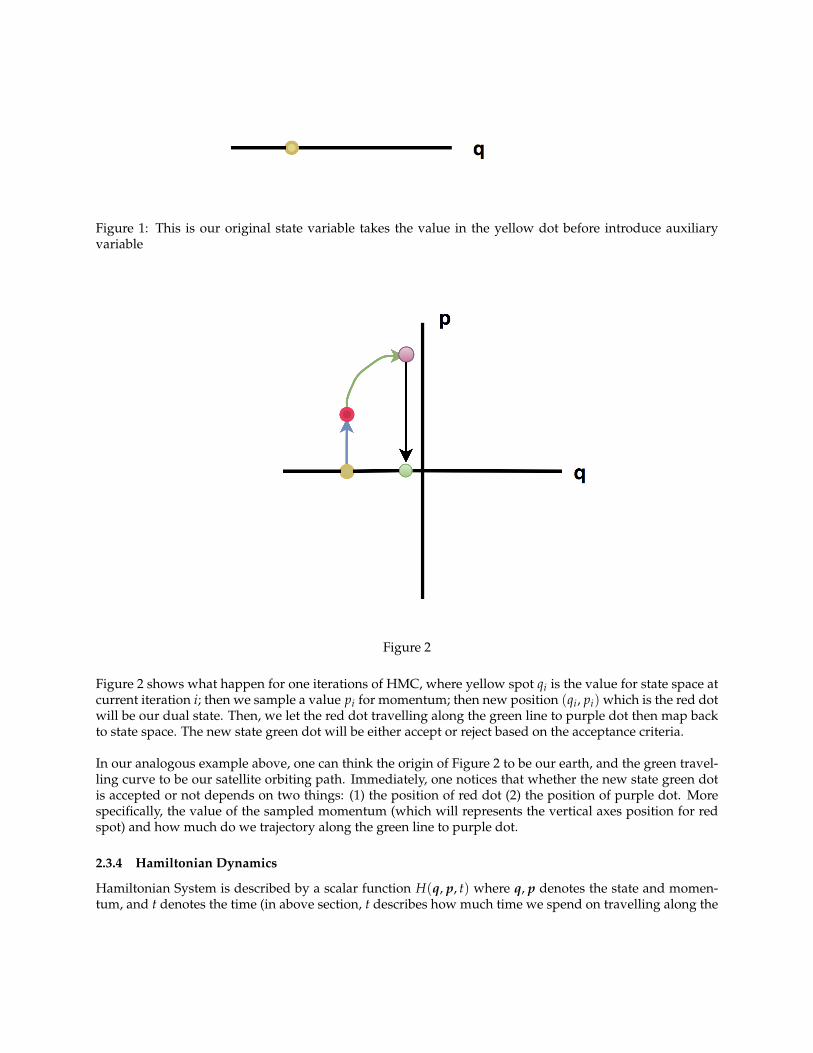
Figure 1: This is our original state variable takes the value in the yellow dot before introduce auxiliaryvariable

Figure 2

Figure 2 shows what happen for one iterations of HMC, where yellow spot qi is the value for state space atcurrent iteration i; then we sample a value pi for momentum; then new position (qi, pi) which is the red dotwill be our dual state. Then, we let the red dot travelling along the green line to purple dot then map backto state space. The new state green dot will be either accept or reject based on the acceptance criteria.

In our analogous example above, one can think the origin of Figure 2 to be our earth, and the green travel-ling curve to be our satellite orbiting path. Immediately, one notices that whether the new state green dotis accepted or not depends on two things: (1) the position of red dot (2) the position of purple dot. Morespecifically, the value of the sampled momentum (which will represents the vertical axes position for redspot) and how much do we trajectory along the green line to purple dot.

2.3.4 Hamiltonian Dynamics

Hamiltonian System is described by a scalar function H(q, p, t) where q, p denotes the state and momen-tum, and t denotes the time (in above section, t describes how much time we spend on travelling along the

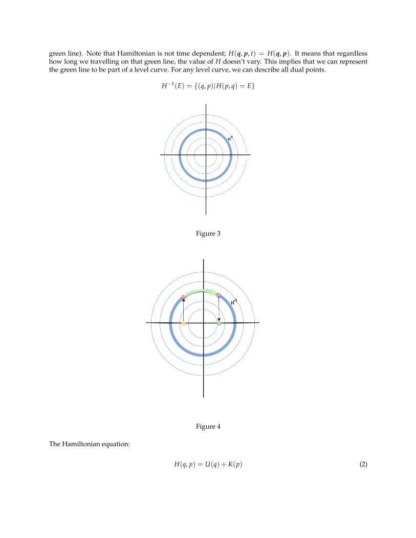
green line). Note that Hamiltonian is not time dependent; H(q, p, t) = H(q, p). It means that regardlesshow long we travelling on that green line, the value of H doesn’t vary. This implies that we can representthe green line to be part of a level curve. For any level curve, we can describe all dual points.

H−1(E) = {(q, p)|H(p, q) = E}

Figure 3

Figure 4

The Hamiltonian equation:

H(q, p) = U(q) + K(p) (2)

Where potential function U(q) is minus log of interest un-normalized density; while kinetic function K(p)is choice of our own. In general, the most standard choice of K would be

K(p) =pT M−1 p

2(3)

Where M is a symmetric semi-definite mass matrix. We usually use matrix M as co-variance matrix formomentum distribution. So we can think of momentum has distribution p ∼ Gaussian(0, M).Define the joint distribution of momentum and state to be as

π(q, p) ∼ exp(−H(q, p)/T) (4)

This joint probability is in form of Canonical ensemble, it can help us to sample a point on any given levelcurve. Then one can perform marginalization π(q) = ∑p π(q|p)π(p). T is the hyper-parameter called tem-perature.

Hamiltonian dynamics can also be understood as the result from a certain set of differential equationssatisfies the following two conditions

dqdt

=∂H∂p

(5)

dpdt

= −∂H∂q

(6)

In HMC, we would have the following results:

dqdt

= M−1 p (7)

dpdt

= −∂U∂q

(8)

Solving the above differential equation, one can derive the function q(t), p(t). This two functions will tellus the value of (q, p) for each time on a given level curve.

2.3.5 Leapfrog

Once we define our probability distribution for momentum, we need the method of trajectory; namely, howdo we traveling along a given level curve. As shown above, travelling along the level curve is equivalentto solve the differential equations of (7), (8). Leapfrog is an iterative method of numerical integration thatupdating q, p at each time step. During the iteration, we can collect all approximated values of (q, p) along

the curve. The leapfrog method is as follows:

Algorithm 1: Leapfroginput : step size ε, step length L, initial position (q0, p0)p = p0 − ε ∗ ∂U

∂q (q0)/2for i : 1→ L do

q← q + ε ∗ pp← p− ε ∗ ∂U

∂q (q)endp = p− ε ∗ ∂U

∂q (q)/2return (q,−p); // negation of momemtum isn’t part of leapfrog but in HMC, it’s used forproposal symmetric

2.3.6 Simple HMC Algorithm

Just like all other MCMC method, there is criteria for the newly sampled state to be accepted or not. Startswith (q0, p0), by performing leapfrog method, we will have a updated proposed dual point (q, p) that is atend of the travelling along the level curve. This proposed point is accepted as next state with probability

Algorithm 2: AcceptanceCriteria

input : proposed position (q, p), initial state (q0, p0)u ∼ uni f (0, 1)if u < exp(−H(q, p) + H(q0, p0)) then

return qendelse

return q0end

If the proposed state is not accepted, the next state is the same as the current state. The full algorithm isperformed as follow:

Algorithm 3: Simple HMCinput : initial state q0, step size ε, step length L, num of iterations N,mass matrix M, potential Ui = 0p0 ∼ N(0, M)S = {} ; // set to save all sampleswhile i < N do

(q, p)← Leap f rog(ε, L, (q0, p0))q← AcceptanceCriteria((q, p), (q0, p0))S← S ∪ {q}p0 ∼ N(0, M) ; // sample a new momentumq0 ← q ; // update the current statei ++

endreturn (q, p)

3 Variation on Simple HMC

3.1 Motivation for Variation

3.1.1 The Importance of Hyper-parameters

We see that the result of Hamiltonian MC is very sensitive to many hyper-parameters; it highly depends ontrajectory length L, step size ε, and our choice of kinetic function K, namely, the mass matrix M.

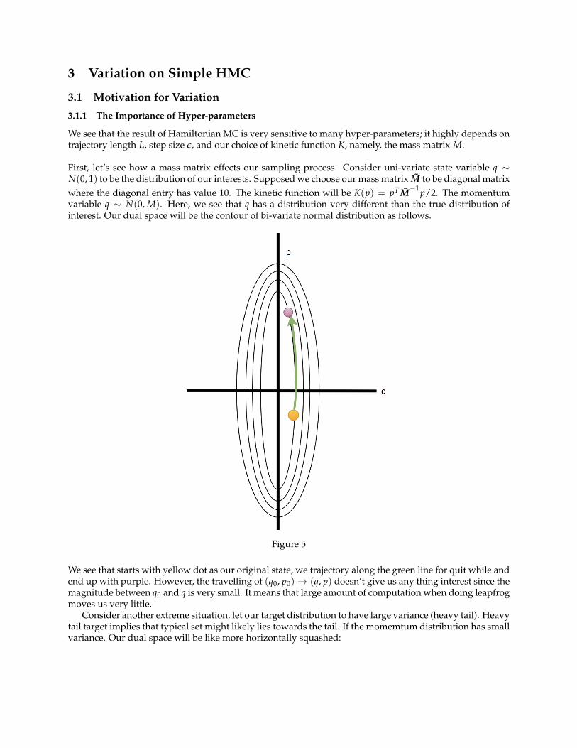
First, let’s see how a mass matrix effects our sampling process. Consider uni-variate state variable q ∼N(0, 1) to be the distribution of our interests. Supposed we choose our mass matrix M to be diagonal matrixwhere the diagonal entry has value 10. The kinetic function will be K(p) = pT M−1 p/2. The momentumvariable q ∼ N(0, M). Here, we see that q has a distribution very different than the true distribution ofinterest. Our dual space will be the contour of bi-variate normal distribution as follows.

Figure 5

We see that starts with yellow dot as our original state, we trajectory along the green line for quit while andend up with purple. However, the travelling of (q0, p0)→ (q, p) doesn’t give us any thing interest since themagnitude between q0 and q is very small. It means that large amount of computation when doing leapfrogmoves us very little.

Consider another extreme situation, let our target distribution to have large variance (heavy tail). Heavytail target implies that typical set might likely lies towards the tail. If the momemtum distribution has smallvariance. Our dual space will be like more horizontally squashed:

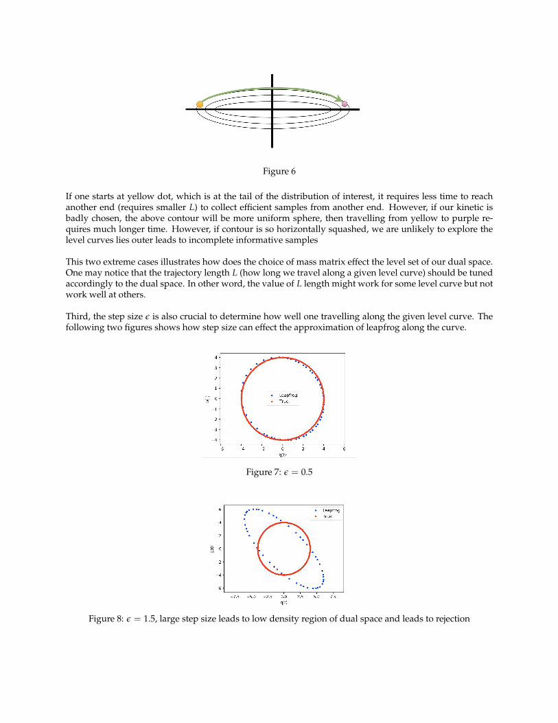
Figure 6

If one starts at yellow dot, which is at the tail of the distribution of interest, it requires less time to reachanother end (requires smaller L) to collect efficient samples from another end. However, if our kinetic isbadly chosen, the above contour will be more uniform sphere, then travelling from yellow to purple re-quires much longer time. However, if contour is so horizontally squashed, we are unlikely to explore thelevel curves lies outer leads to incomplete informative samples

This two extreme cases illustrates how does the choice of mass matrix effect the level set of our dual space.One may notice that the trajectory length L (how long we travel along a given level curve) should be tunedaccordingly to the dual space. In other word, the value of L length might work for some level curve but notwork well at others.

Third, the step size ε is also crucial to determine how well one travelling along the given level curve. Thefollowing two figures shows how step size can effect the approximation of leapfrog along the curve.

Figure 7: ε = 0.5

Figure 8: ε = 1.5, large step size leads to low density region of dual space and leads to rejection

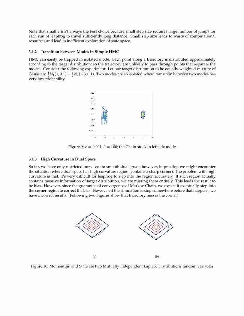
Note that small ε isn’t always the best choice because small step size requires large number of jumps foreach run of leapfrog to travel sufficiently long distance. Small step size leads to waste of computationalresources and lead to inefficient exploration of state space.

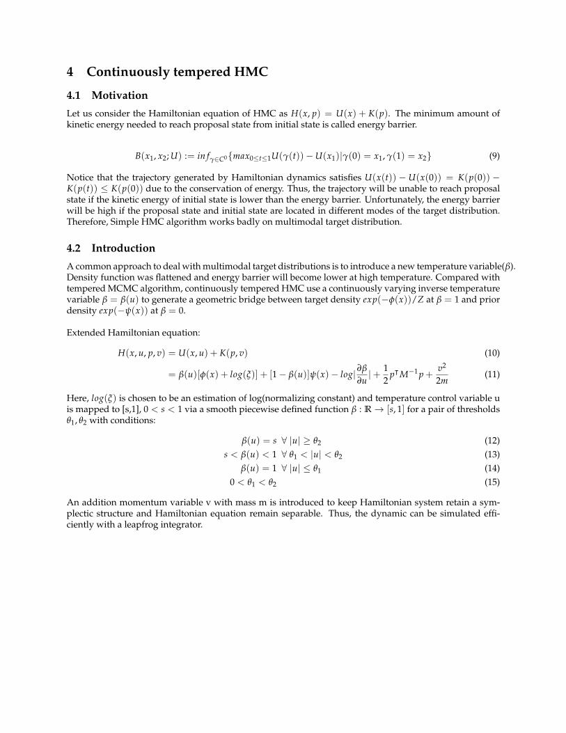
3.1.2 Transition between Modes in Simple HMC

HMC can easily be trapped in isolated mode. Each point along a trajectory is distributed approximatelyaccording to the target distribution; so the trajectory are unlikely to pass through points that separate themodes. Consider the following experiment: Let our target distribution to be equally weighted mixture ofGaussian: 1

2 N1(1, 0.1) + 12 N2(−3, 0.1). Two modes are so isolated where transition between two modes has

very low probability.

Figure 9: ε = 0.001, L = 100; the Chain stuck in leftside mode

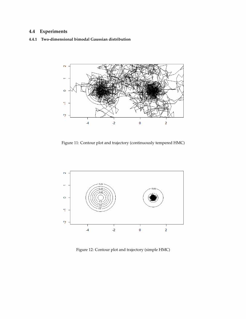
3.1.3 High Curvature in Dual Space

So far, we have only restricted ourselves to smooth dual space; however, in practice, we might encounterthe situation where dual space has high curvature region (contains a sharp corner). The problem with highcurvature is that, it’s very difficult for leapfrog to step into the region accurately. If such region actuallycontains massive information of target distribution, we are missing them entirely. This leads the result tobe bias. However, since the guarantee of convergence of Markov Chain, we expect it eventually step intothe corner region to correct the bias. However, if the simulation is stop somewhere before that happens, wehave incorrect results. (Following two Figures show that trajectory misses the corner)

(a) (b)

Figure 10: Momentum and State are two Mutually Independent Laplace Distributions random variables

4 Continuously tempered HMC

4.1 Motivation

Let us consider the Hamiltonian equation of HMC as H(x, p) = U(x) + K(p). The minimum amount ofkinetic energy needed to reach proposal state from initial state is called energy barrier.

B(x1, x2; U) := in fγ∈C0{max0≤t≤1U(γ(t))−U(x1)|γ(0) = x1, γ(1) = x2} (9)

Notice that the trajectory generated by Hamiltonian dynamics satisfies U(x(t)) − U(x(0)) = K(p(0)) −K(p(t)) ≤ K(p(0)) due to the conservation of energy. Thus, the trajectory will be unable to reach proposalstate if the kinetic energy of initial state is lower than the energy barrier. Unfortunately, the energy barrierwill be high if the proposal state and initial state are located in different modes of the target distribution.Therefore, Simple HMC algorithm works badly on multimodal target distribution.

4.2 Introduction

A common approach to deal with multimodal target distributions is to introduce a new temperature variable(β).Density function was flattened and energy barrier will become lower at high temperature. Compared withtempered MCMC algorithm, continuously tempered HMC use a continuously varying inverse temperaturevariable β = β(u) to generate a geometric bridge between target density exp(−φ(x))/Z at β = 1 and priordensity exp(−ψ(x)) at β = 0.

Extended Hamiltonian equation:

H(x, u, p, v) = U(x, u) + K(p, v) (10)

= β(u)[φ(x) + log(ξ)] + [1− β(u)]ψ(x)− log|∂β

∂u|+ 1

2pᵀM−1 p +

v2

2m(11)

Here, log(ξ) is chosen to be an estimation of log(normalizing constant) and temperature control variable uis mapped to [s,1], 0 < s < 1 via a smooth piecewise defined function β : R→ [s, 1] for a pair of thresholdsθ1, θ2 with conditions:

β(u) = s ∀ |u| ≥ θ2 (12)s < β(u) < 1 ∀ θ1 < |u| < θ2 (13)

β(u) = 1 ∀ |u| ≤ θ1 (14)0 < θ1 < θ2 (15)

An addition momentum variable v with mass m is introduced to keep Hamiltonian system retain a sym-plectic structure and Hamiltonian equation remain separable. Thus, the dynamic can be simulated effi-ciently with a leapfrog integrator.

4.3 Algorithm

Algorithm 4: Leapfroginput : step size ε, step length L, initial position (q0, u0, p0, v0)p′ = (p, v)q′ = (q, u)p′ = p′0 − ε× ∂U

∂q′ (q′0)/2

for i : 1→ L doq′ ← q′ + ε× p′

if i! = L thenp′ ← p′ − ε× ∂U

∂q′ (q′)

endendp′ = p′ − ε ∗ ∂U

∂q′ (q′)/2

return (q′,−p′)

Algorithm 5: Acceptance Criteria

input : proposed position (q′, p′), initial state (q′0, p′0) = (q0, u0, p0, v0)u ∼ uni f (0, 1)if log(u) < −H(q′, p′) + H(q′0, p′0) then

return q′

endelse

return q′0end

If the proposed state is not accepted, the next state is the same as the current state. The full algorithm isperformed as follow:

Algorithm 6: Continuously tempered HMC

input : initial state q′0, step size ε, step length L, num of iterations N,mass matrix M, potential U,kinetic K, coefficient c

i = 0p0 ∼ N(0, M) ; // M is a squared matrix with nrow = dim+1S = {} ; // set to save all sampleswhile i < N do

(q′, p′)← Leap f rog(c, ε, L, (q′0, p′0))q′ ← AcceptanceCriteria((q′, p′), (q′0, p′0))S← S ∪ {q′}p∗ ∼ N(0, M)

p′0 ← c× p∗ +√

1− c2 × p′0; // Partially/fully resample a new momentumq′0 ← q′ ; // update the current statei ++

endreturn (q′, p′)

4.4 Experiments

4.4.1 Two-dimensional bimodal Gaussian distribution

Figure 11: Contour plot and trajectory (continuously tempered HMC)

Figure 12: Contour plot and trajectory (simple HMC)

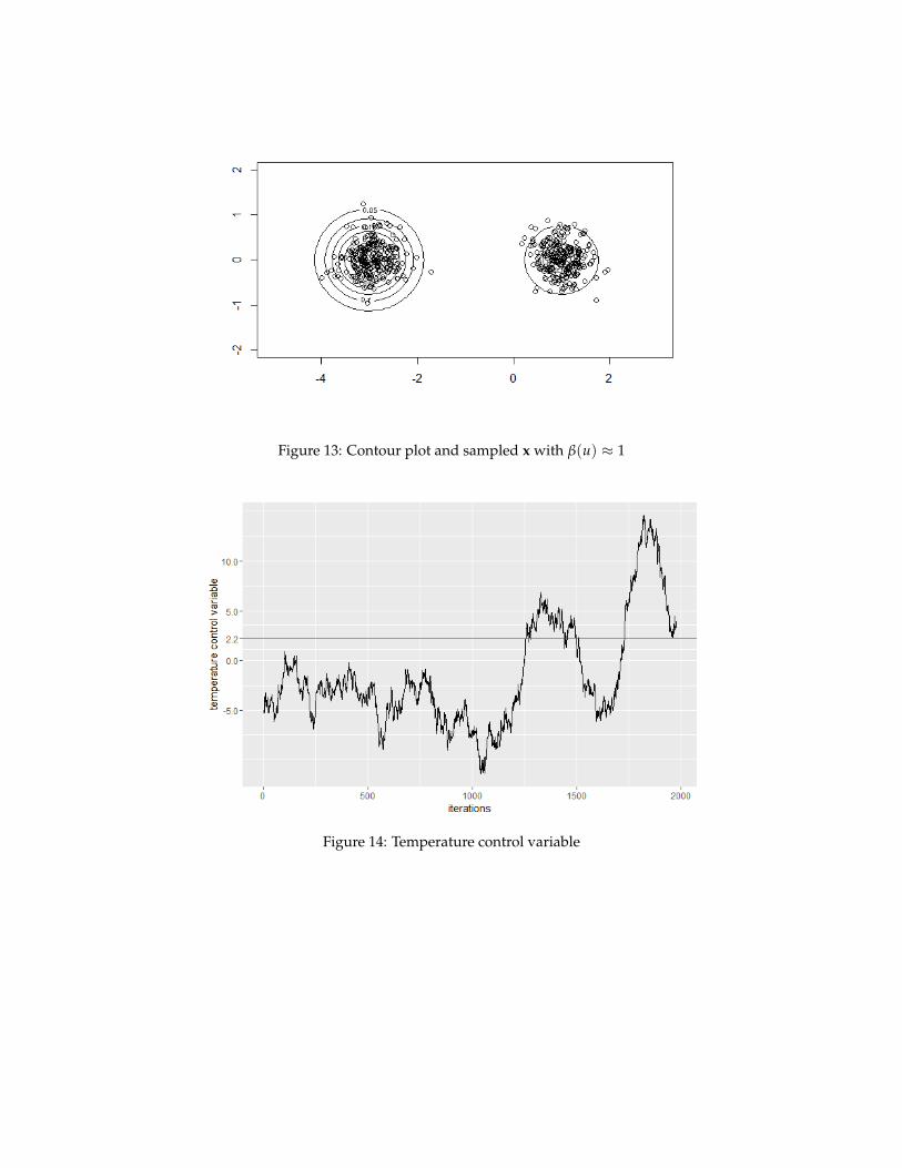
Figure 13: Contour plot and sampled x with β(u) ≈ 1

Figure 14: Temperature control variable

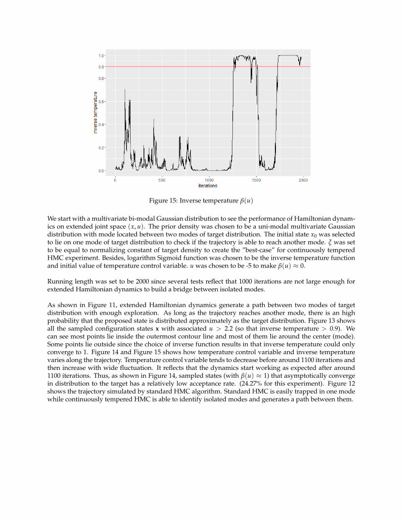
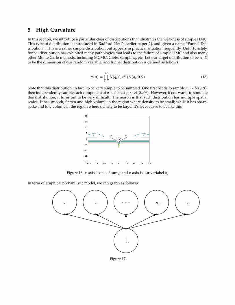
Figure 15: Inverse temperature β(u)

We start with a multivariate bi-modal Gaussian distribution to see the performance of Hamiltonian dynam-ics on extended joint space (x, u). The prior density was chosen to be a uni-modal multivariate Gaussiandistribution with mode located between two modes of target distribution. The initial state x0 was selectedto lie on one mode of target distribution to check if the trajectory is able to reach another mode. ξ was setto be equal to normalizing constant of target density to create the ”best-case” for continuously temperedHMC experiment. Besides, logarithm Sigmoid function was chosen to be the inverse temperature functionand initial value of temperature control variable. u was chosen to be -5 to make β(u) ≈ 0.

Running length was set to be 2000 since several tests reflect that 1000 iterations are not large enough forextended Hamiltonian dynamics to build a bridge between isolated modes.

As shown in Figure 11, extended Hamiltonian dynamics generate a path between two modes of targetdistribution with enough exploration. As long as the trajectory reaches another mode, there is an highprobability that the proposed state is distributed approximately as the target distribution. Figure 13 showsall the sampled configuration states x with associated u > 2.2 (so that inverse temperature > 0.9). Wecan see most points lie inside the outermost contour line and most of them lie around the center (mode).Some points lie outside since the choice of inverse function results in that inverse temperature could onlyconverge to 1. Figure 14 and Figure 15 shows how temperature control variable and inverse temperaturevaries along the trajectory. Temperature control variable tends to decrease before around 1100 iterations andthen increase with wide fluctuation. It reflects that the dynamics start working as expected after around1100 iterations. Thus, as shown in Figure 14, sampled states (with β(u) ≈ 1) that asymptotically convergein distribution to the target has a relatively low acceptance rate. (24.27% for this experiment). Figure 12shows the trajectory simulated by standard HMC algorithm. Standard HMC is easily trapped in one modewhile continuously tempered HMC is able to identify isolated modes and generates a path between them.

5 High Curvature

In this section, we introduce a particular class of distributions that illustrates the weakness of simple HMC.This type of distribution is introduced in Radford Neal’s earlier paper[2], and given a name ”Funnel Dis-tribution”. This is a rather simple distribution but appears in practical situation frequently. Unfortunately,funnel distribution has exhibited many pathologies that leads to the failure of simple HMC and also manyother Monte Carlo methods, including MCMC, Gibbs Sampling, etc. Let our target distribution to be π, Dto be the dimension of our random variable, and funnel distribution is defined as follows:

π(q) =D

∏i=1

N(qi|0, eq0)N(q0|0, 9) (16)

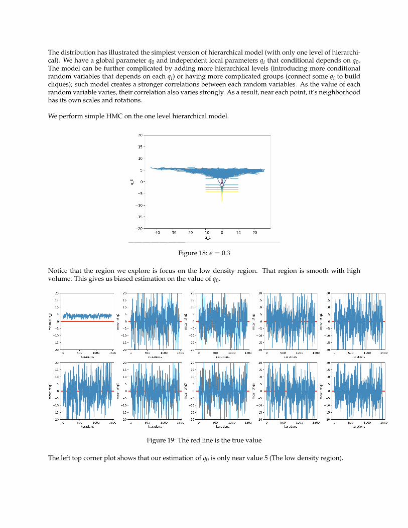
Note that this distribution, in face, to be very simple to be sampled. One first needs to sample q0 ∼ N(0, 9),then independently sample each component of q such that qi ∼ N(0, eq0). However, if one wants to simulatethis distribution, it turns out to be very difficult. The reason is that such distribution has multiple spatialscales. It has smooth, flatten and high volume in the region where density to be small; while it has sharp,spike and low volume in the region where density to be large. It’s level curve to be like this

Figure 16: x-axis is one of our qi and y-axis is our variabel q0

In term of graphical probabilistic model, we can graph as follows:

Figure 17

The distribution has illustrated the simplest version of hierarchical model (with only one level of hierarchi-cal). We have a global parameter q0 and independent local parameters qi that conditional depends on q0.The model can be further complicated by adding more hierarchical levels (introducing more conditionalrandom variables that depends on each qi) or having more complicated groups (connect some qi to buildcliques); such model creates a stronger correlations between each random variables. As the value of eachrandom variable varies, their correlation also varies strongly. As a result, near each point, it’s neighborhoodhas its own scales and rotations.

We perform simple HMC on the one level hierarchical model.

Figure 18: ε = 0.3

Notice that the region we explore is focus on the low density region. That region is smooth with highvolume. This gives us biased estimation on the value of q0.

Figure 19: The red line is the true value

The left top corner plot shows that our estimation of q0 is only near value 5 (The low density region).

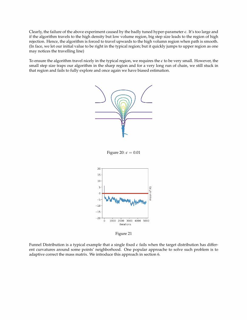
Clearly, the failure of the above experiment caused by the badly tuned hyper-parameter ε. It’s too large andif the algorithm travels to the high density but low volume region, big step size leads to the region of highrejection. Hence, the algorithm is forced to travel upwards to the high volumn region when path is smooth.(In face, we let our initial value to be right in the typical region; but it quickly jumps to upper region as onemay notices the travelling line)

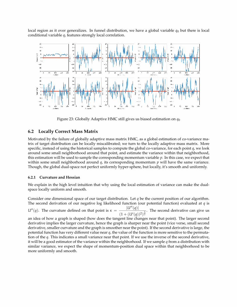
To ensure the algorithm travel nicely in the typical region, we requires the ε to be very small. However, thesmall step size traps our algorithm in the sharp region and for a very long run of chain, we still stuck inthat region and fails to fully explore and once again we have biased estimation.

Figure 20: ε = 0.01

Figure 21

Funnel Distribution is a typical example that a single fixed ε fails when the target distribution has differ-ent curvatures around some points’ neighborhood. One popular approache to solve such problem is toadaptive correct the mass matrix. We introduce this approach in section 6.

6 Riemannian HMC

As mention earlier, when we introduce momentum variable into our model, our algorithm will be travellingin the duel space. When the target has high curvature region, by choose the correct mass matrix (co-variancematrix for momentum variable), the resulting dual space will be less likely to have high curvature. In face,with perfect choice of mass matrix, we will end up with a perfect uniformly hyper-sphere dual space, wherethe exploration space is smooth with same curvature everywhere. The perfect uniformly hyper-sphere dualspace occurs when the momentum distribution happens to be exactly of our target distribution.

6.1 Globally Correct Mass Matrix

Based on above idea, we starts with a naive approach of mass matrix adaptive method. Let the chainruns for several iterations, then use the most recent samples collected to estimate the empirical co-variancematrix of the target distribution, then change our mass matrix to be this empirical estimation and sampleour momentum from this new co-variance matrix.

Algorithm 7: Global Adaptive Mass Matrix HMCi← 0S← {}while not converge do

Run a single iteration of Simple HMCS← S ∪ {qi} ; // Collect the sample from this iteration run of HMCi← i + 1if i% 1000 == 0 ; // Estimate the target co-variance every 1000 iterationsthen

M ← Covaraince(S); // Sample covariance matrix; then use it as new mass matrix

endend

Figure 22: ε = 0.3 with global adaptive mass matrix HMC

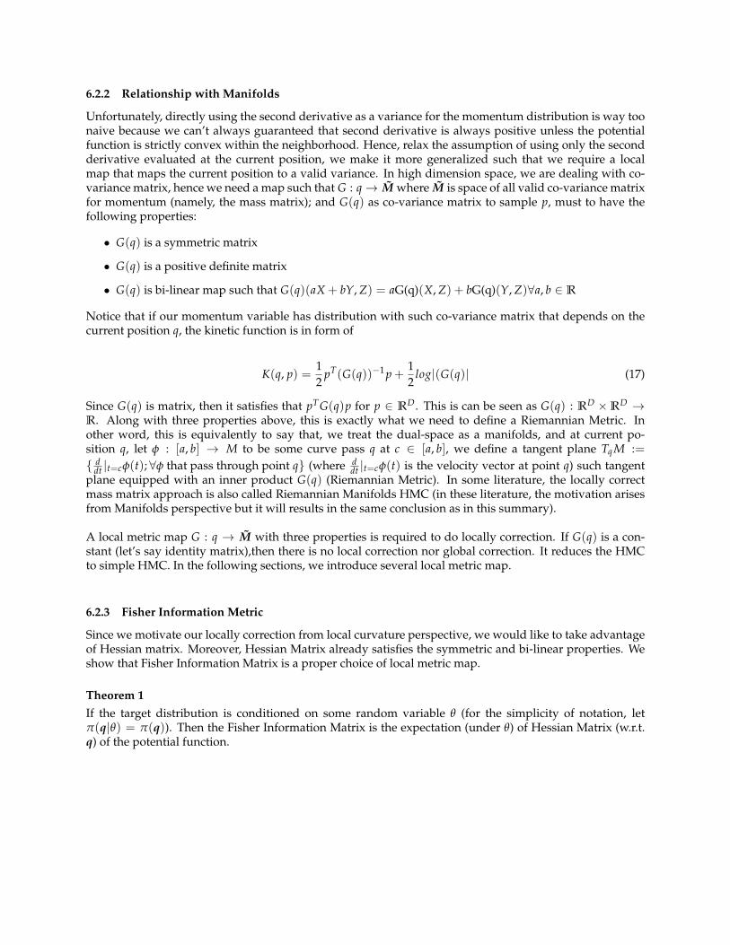
Unfortunately, this doesn’t gives us a good result; in face, it doesn’t improve compared to our simple HMCat all. We still have the biased estimation of q0. The very reason is that the funnel distribution is notglobal correlations. Every time when we estimate the target distribution, we use all of the past samplesand approximate a global co-variance matrix of the target distribution; which it can estimate badly in the

local region as it over generalizes. In funnel distribution, we have a global variable q0 but there is localconditional variable qi features strongly local correlation.

Figure 23: Globally Adaptive HMC still gives us biased estimation on q0

6.2 Locally Correct Mass Matrix

Motivated by the failure of globally adaptive mass matrix HMC, as a global estimation of co-variance ma-trix of target distribution can be locally miscalibrated; we turn to the locally adaptive mass matrix. Morespecific, instead of using the historical samples to compute the global co-variance, for each point q, we lookaround some small neighborhood around that point, and estimate the variance within that neighborhood,this estimation will be used to sample the corresponding momentum variable p. In this case, we expect thatwithin some small neighborhood around q, its corresponding momentum p will have the same variance.Though, the global dual-space not perfect uniformly hyper-sphere, but locally, it’s smooth and uniformly.

6.2.1 Curvature and Hessian

We explain in the high level intuition that why using the local estimation of variance can make the dual-space locally uniform and smooth.

Consider one dimensional space of our target distribution. Let q be the current position of our algorithm.The second derivation of our negative log likelihood function (our potential function) evaluated at q is

U′′(q). The curvature defined on that point is κ =|U′′(q)|

(1 + (U′(q))2)32

. The second derivative can give us

an idea of how a graph is shaped (how does the tangent line changes near that point). The larger secondderivative implies the larger curvature, hence the graph is sharper near the point (vice verse, small secondderivative, smaller curvature and the graph is smoother near the point). If the second derivative is large, thepotential function has very different value near q, the value of the function is more sensitive to the permuta-tion of the q. This indicates a small variance near that point. If we use the inverse of the second derivative,it will be a good estimator of the variance within the neighborhood. If we sample q from a distribution withsimilar variance, we expect the shape of momentum-position dual space within that neighborhood to bemore uniformly and smooth.

6.2.2 Relationship with Manifolds

Unfortunately, directly using the second derivative as a variance for the momentum distribution is way toonaive because we can’t always guaranteed that second derivative is always positive unless the potentialfunction is strictly convex within the neighborhood. Hence, relax the assumption of using only the secondderivative evaluated at the current position, we make it more generalized such that we require a localmap that maps the current position to a valid variance. In high dimension space, we are dealing with co-variance matrix, hence we need a map such that G : q→ M where M is space of all valid co-variance matrixfor momentum (namely, the mass matrix); and G(q) as co-variance matrix to sample p, must to have thefollowing properties:

• G(q) is a symmetric matrix

• G(q) is a positive definite matrix

• G(q) is bi-linear map such that G(q)(aX + bY, Z) = aG(q)(X, Z) + bG(q)(Y, Z)∀a, b ∈ R

Notice that if our momentum variable has distribution with such co-variance matrix that depends on thecurrent position q, the kinetic function is in form of

K(q, p) =12

pT(G(q))−1 p +12

log|(G(q)| (17)

Since G(q) is matrix, then it satisfies that pTG(q)p for p ∈ RD. This is can be seen as G(q) : RD ×RD →R. Along with three properties above, this is exactly what we need to define a Riemannian Metric. Inother word, this is equivalently to say that, we treat the dual-space as a manifolds, and at current po-sition q, let φ : [a, b] → M to be some curve pass q at c ∈ [a, b], we define a tangent plane Tq M :={ d

dt |t=cφ(t); ∀φ that pass through point q} (where ddt |t=cφ(t) is the velocity vector at point q) such tangent

plane equipped with an inner product G(q) (Riemannian Metric). In some literature, the locally correctmass matrix approach is also called Riemannian Manifolds HMC (in these literature, the motivation arisesfrom Manifolds perspective but it will results in the same conclusion as in this summary).

A local metric map G : q → M with three properties is required to do locally correction. If G(q) is a con-stant (let’s say identity matrix),then there is no local correction nor global correction. It reduces the HMCto simple HMC. In the following sections, we introduce several local metric map.

6.2.3 Fisher Information Metric

Since we motivate our locally correction from local curvature perspective, we would like to take advantageof Hessian matrix. Moreover, Hessian Matrix already satisfies the symmetric and bi-linear properties. Weshow that Fisher Information Matrix is a proper choice of local metric map.

Theorem 1If the target distribution is conditioned on some random variable θ (for the simplicity of notation, letπ(q|θ) = π(q)). Then the Fisher Information Matrix is the expectation (under θ) of Hessian Matrix (w.r.t.q) of the potential function.

Proof.

∇2qU(q) = ∇2

q − log(q) (18)

= ∇(∇π(q)π(q)

) (19)

=π(q)∇2π(q)−∇π(q)∇π(q)T

π(q)2 (20)

=π(q)∇2π(q)

π(q)2 − ∇π(q)∇π(q)T

π(q)2 (21)

Take the Expectation under. θ on both side yields

E(∇2qU(q)) = −E(

π(q)∇2π(q)π(q)2 − ∇π(q)∇π(q)T

π(q)2 ) (22)

= −(E(π(q)∇2π(q)

π(q)2 )−E(∇π(q)∇π(q)T

π(q)2 )) (23)

= −( ∫∇2π(q)

)−E(∇log(π(q))∇log(π(q))T) (24)

= −(∇2

∫π(q)

)+ E(∇log(π(q))∇log(π(q))T) (25)

= E(∇log(π(q))∇log(π(q))T) (26)

The equation(26) is the definition of Fisher Information.

Theorem 2The Fisher Information Matrix is positive semi-definite.

Proof. Let Iij = Eθ [(∇ log π(q)) (∇ log π(q))]; and let u = (u1, . . . , uD)> ∈ RD be some nonzero vector

D

∑i,j=1

ui Iijuj =D

∑i,j=1

(uiEθ

[(∂i log π(q))

(∂j log π(q)

)]uj)

(27)

= Eθ

[(D

∑i=1

ui∂i log π(q)

)(D

∑j=1

uj∂j log π(q)

)](28)

= Eθ

( D

∑i=1

ui∂i log π(q)

)2 ≥ 0 . (29)

Equation (26) also gives us an advantage in term of computational complexity. When compute the Hes-sian Matrix of potential function to be tedious, one can compute its gradient and take the dot product(Theright hand side). Unfortunately, there are few short-cuts of such choice of local metric. First, the Fisher In-formation is only positive semi-definite, and still can be singular and leads to invalid values. Secondly,evaluating expectation over random variable θ will not be practical. Even we compute the empiricalFisher 1

S ∑i p(θi)π(q|θi). We need to know the distribution p(θ). Unless the target distribution is naturallyequipped with such conditional random variable θ with a simple distribution to sample it, we couldn’t takesuch advantages.

6.2.4 Soft Absolute Metric

This is a more generalized metric introduced by Betancourt[4] that relax the assumption of the conditionalrandom variable requirement in Fisher Information metric and also forces the metric to be positive definite.

The Hessian matrix H is symmetric; by Spectral Theorem, it can be diagonalized as H = QΛQT whereQ is a matrix consists of orthonormalized eigenvectors and Λ is a diagonal matrix where the diagonal isthe corresponding eigenvalues. Also note that, when all the eigenvalues are positive, then H must be apositive definite matrix. The idea lies in Soft Absolute Metric is that designing a differentiable functionφ to approximate the absolute value function. We apply function φ to each of eigenvalues to force theeigenvalues to be positive. Moreover, we want to regularize the small value of eigenvalues to avoid thenumerical instability. The approximation map is

φ(λ) = λexp(aλ) + exp(−aλ)

exp(aλ)− exp(−aλ)(30)

Since exponential function positive all time, it assures that even when the true absolute value of λ is soclose to zero, the transformed λ is bounded below by some positive number. The value of a > 0 is theapproximation control that controls how close we want our map φ to be with true absolute function. Asa→ ∞, φ(λ)→ |λ|.

One needs to be more careful when implement the soft absolute metric as the exponential function mightbe easily explode and leads to numerical overflow. A more numerical stable implementation is as follows:

If λ > 0, then multiply both of the denominator and numerator by exp(aλ); then equation (30) becomes

φ(λ) = λ1 + exp(−2aλ)

1− exp(−2aλ)(31)

If λ < 0, then multiply both of the denominator and numerator by exp(−aλ); then equation (30) becomes

φ(λ) = λexp(2aλ) + 1exp(2aλ)− 1

(32)

The Soft Absolute Metric will be φ(H) = Qφ(Λ)QT . The approximation control a can be set as hyper-parameter or it can be automatically adapted through the training based on the acceptance rate.

6.2.5 Smooth Metric

Based the same idea, we introduce another general metric called Smooth Metric. It is almost same as SoftAbsolute Metric with one thing different. We use a different absolute value function approximation.

ψ(λ) = (λ2 + a2)1/2 (33)

As a → 0, ψ(λ) → |λ| and the function is bounded below by a. The approximator will be narrower thanthe Soft Metric so that for each λ, its approximated value will be slighter larger than the Soft Metric andfurther reduces the possibility of the numerical instability.

6.3 Locally Correction Algorithm

6.3.1 General Form

Let G(q) be a local metric we choose. Now the kinetic function will be position-dependent and has the formof

K(q, p) =12

pTG(q)−1 p +12

log|G(q)| (34)

The Hamiltonian joint distribution becomes

H(q, p) = U(q) + K(q, p) (35)

The sampling process is can be written as Gibbs sampling as

q∗|p ∼ N(0, G(q)) (36)p∗|q∗ ∝ exp(−H(q∗ + δq∗, p∗)) (37)

The momentum-position dual variable (q∗ + δq∗, p∗) is obtained through performing leapfrog algorithm.Note that Simple HMC leapfrog no longer will be working here because now, kinetic function involvesvariable q, the Hamiltonian is non-separable, implies that ∂q H requires differentiate through K(q, p). Andthis needed to be taken into consideration when doing leapfrog. Here, we adopt the generalized leapfrogalgorithm[5]

pn+1/2 ← pn − ε

2∂qH(qn, pn+1/2) (38)

qn+1 ← qn +ε

2[∂pH(qn, pn+1/2) + ∂p H(qn+1, pn+1/2)] (39)

pn+1 ← pn+1/2 − ε

2∂qH(qn+1, pn+1/2) (40)

6.3.2 Fixed Point Method

Note, equation (38) and equation (39) are defined implicitly.Use fixed point iteration. In more general case,we are solving situation like g(x) = x Randomly choose a point x0, consider a recursive process

xn+1 = g(xn)

Theoretically, if g(x)− x is a continuous function and {xn} converges, then it converges to the solution ofg(x) = x. Hence, equation (38) and (39) will be solved through such recursive method. (the number ofiteration is a hyper-parameters we choose beforehand)

Algorithm 8: Local Correct Mass Matrix HMCinput : G : a specified local metric;

ε : step-size;I : iteration for fixed point method;q0 : the inital position;U : the potentila function;N : the number of interested samples

output: S : a set of samples obtained from HMCj← 0S← {}for j < N do

q0 ∼ N(0, G(q0)) ; // Sample a new momentumL ∼ randint(2, 200) ; // Sample a positive integer for number of leapfrogfor i < L do

p← p0q← q0Perform equation (38) for I number of times to update qPerform equation (39) for I number of times to update pPerform equation (40) for a single time to update q

endu ∼ uni f orm(0, 1)r ← −log(H(q, p)) + log(H(q0, p0))if r > log(u) then

; // Accept the proposed new positionS← S ∪ {q}q0 ← q

endend

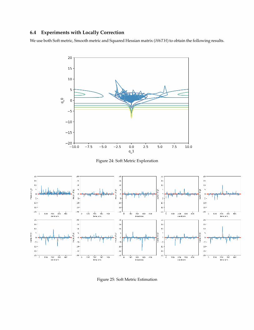
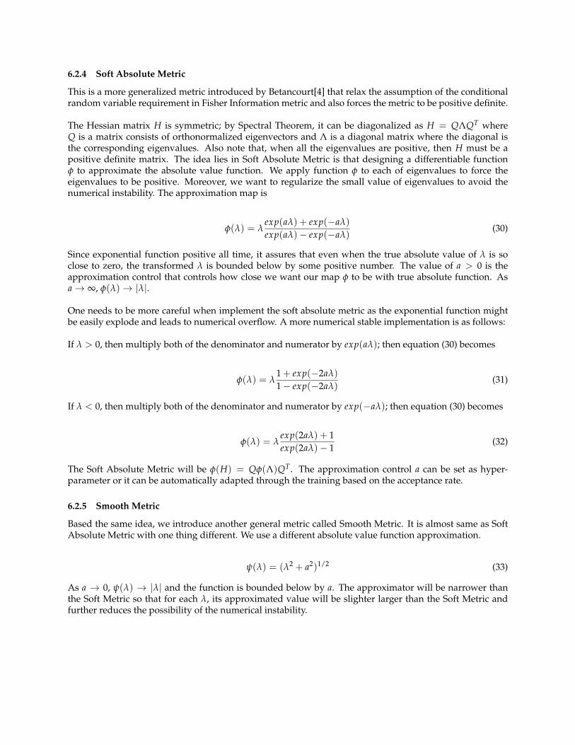
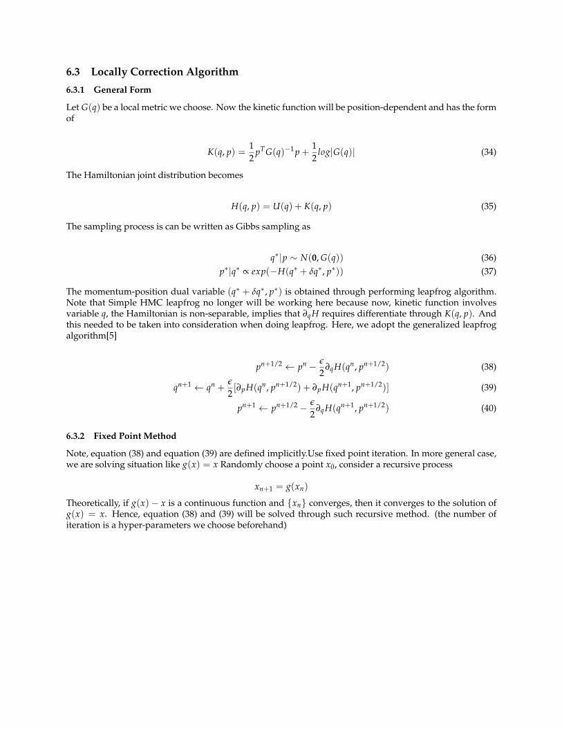
6.4 Experiments with Locally Correction

We use both Soft metric, Smooth metric and Squared Hessian matrix (H6TH) to obtain the following results.

Figure 24: Soft Metric Exploration

Figure 25: Soft Metric Estimation

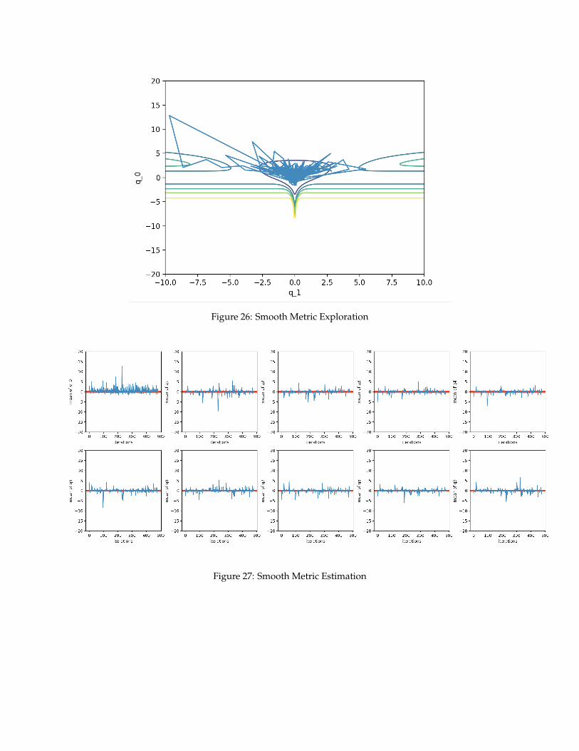
Figure 26: Smooth Metric Exploration

Figure 27: Smooth Metric Estimation

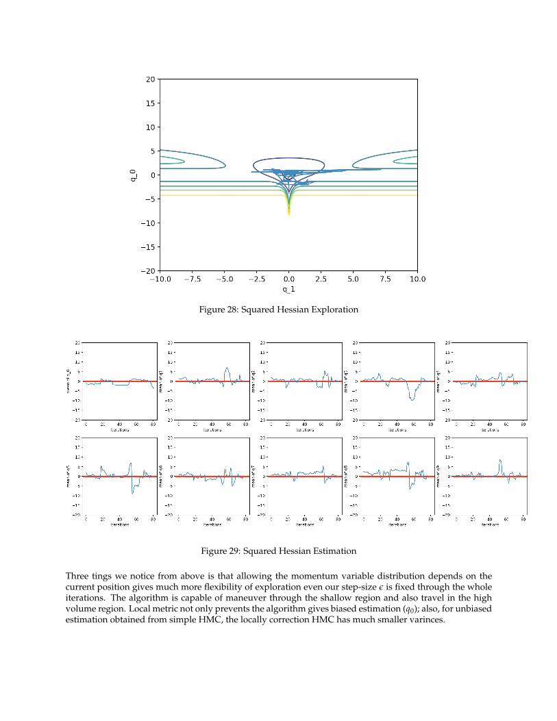
Figure 28: Squared Hessian Exploration

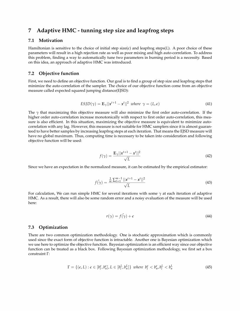
Figure 29: Squared Hessian Estimation

Three tings we notice from above is that allowing the momentum variable distribution depends on thecurrent position gives much more flexibility of exploration even our step-size ε is fixed through the wholeiterations. The algorithm is capable of maneuver through the shallow region and also travel in the highvolume region. Local metric not only prevents the algorithm gives biased estimation (q0); also, for unbiasedestimation obtained from simple HMC, the locally correction HMC has much smaller varinces.

7 Adaptive HMC - tunning step size and leapfrog steps

7.1 Motivation

Hamiltonian is sensitive to the choice of initial step size(ε) and leapfrog steps(L). A poor choice of theseparameters will result in a high rejection rate as well as poor mixing and high auto-correlation. To addressthis problem, finding a way to automatically tune two parameters in burning period is a necessity. Basedon this idea, an approach of adaptive HMC was introduced.

7.2 Objective function

First, we need to define an objective function. Our goal is to find a group of step size and leapfrog steps thatminimize the auto-correlation of the sampler. The choice of our objective function come from an objectivemeasure called expected squared jumping distance(EJSD):

ESJD(γ) = Eγ||xt+1 − xt||2 where γ = (L, ε) (41)

The γ that maximizing this objective measure will also minimize the first order auto-correlation. If thehigher order auto-correlation increase monotonically with respect to first order auto-correlation, this mea-sure is also efficient. In this situation, maximizing the objective measure is equivalent to minimize auto-correlation with any lag. However, this measure is not suitable for HMC samplers since it is almost guaran-teed to have better samples by increasing leapfrog steps at each iteration. That means the EJSD measure willhave no global maximum. Thus, computing time is necessary to be taken into consideration and followingobjective function will be used:

f (γ) =Eγ||xt+1 − xt||2√

L(42)

Since we have an expectation in the normalized measure, it can be estimated by the empirical estimator:

ˆf (γ) =1m ∑m−1

t=1 ||xt+1 − xt||2√

L(43)

For calculation, We can run simple HMC for several iterations with some γ at each iteration of adaptiveHMC. As a result, there will also be some random error and a noisy evaluation of the measure will be usedhere:

r(γ) = ˆf (γ) + ε (44)

7.3 Optimization

There are two common optimization methodology. One is stochastic approximation which is commonlyused since the exact form of objective function is intractable. Another one is Bayesian optimization whichwe use here to optimize the objective function. Bayesian optimization is an efficient way since our objectivefunction can be treated as a black box. Following Bayesian optimization methodology, we first set a boxconstraint Γ:

Γ = {(ε, L) : ε ∈ [bεl , bε

u], L ∈ [bLl , bL

u ]} where bεl < bε

u, bLl < bL

u (45)

Note that ε is a continuous parameter where L is a discrete parameter that is greater than zero. It is nec-essary to discretize it in a very fine grid. For the choice of interval boundaries, they can be set to be largeenough to cover all reasonable γ. A better way is to run adaptive HMC several times and narrow the inter-val.

Since true objective is unknown, we need to find a surrogate model that can be maximized by γ. Here, Weconstruct a Gaussian process to provide a posterior normal distribution over the objective function. First,we specify a prior distribution over the objective function:

f ∼ N(0, k(γi, γj)) (46)

k(γi, γj) is some covariance function with argument γi and γj. Here, we use the Gaussian ARD covariancefunction so that k(γi, γj) = exp(− 1

2 γTi Σ−1γj). At each iteration, we will compute the value of r(γ) and

store the value and γ into a dataset D = {γ, r(γ)}. (at nth iteration, Dn = {{γ}ni=1, {r}n

i=1} ). Given Dk, wecan arrive the posterior distribution over the objective function :

f |Di, γ ∼ N(µi(γ), σ2i (γ)) (47)

µi(γ) = kT(K + σ2 I)−1ri (48)

σ2i (γ) = k(γ, γ)− kT(K + σ2 I)−1k (49)

where k = [k(γ, γ1), ..., k(γ, γi)]T , ri = [r1, ..., ri]

T (50)

K =

k(γ1, γ1) . . . k(γ1, γi)...

. . ....

k(γi, γ1) . . . k(γi, γi)

(51)

Note that the dimension of K will increase as running length increases. This increase the difficulty ofcalculation and decrease efficiency. Thus, we need to carefully choose the number of iterations before theexperiment.Gaussian process enables us to build an acquisition function to tell us which γ maximize the objectivefunction. The function uses the Gaussian process posterior mean to predict regions of potentially higherobjective values and posterior variance to detect regions of high uncertainty (Wang 2013). We use a variantof Upper Confidence bound (UCB) as the acquisition function:

u(γ, s|Di) = µi(γ, s) + piβ12i+1σi(γ) where (52)

µi(γ, s) = µi(γ)× s, pi = (max{i− k + 1, 1})−0.5 (53)

βi+1 = 2log((i + 1)

d2 +2π2

3δ) f or k ∈N+ (54)

pi will continuously decrease to zero after the number of current iterations are greater than k where k wasset to be Burning period B divided by running length of standard HMC at each iteration (m). Thus, Itbecomes increasingly difficult for Bayesian optimization to propose new γ as pi decreases. It is better topredict known good γ with a good initial value rather than exploring a better one.

7.4 Algorithm

Algorithm 9: Adaptive HMCinput : Γ : box constraint;

m : running length of standard HMC at each iteration (Burning period;k, αn : total number of iterationsγ1 : initial value of γ

output: S : a set of samples obtained from HMCS← {}for i = 1, ..., m do

Run standard HMC for m iterations with γi = (εi, Li).Store the drawn samples into SCalculate the value of objective function ri using the drawn samples.Store γi, ri into dataset Diif ri > supj∈{1,...,i−1} then

s = αri

endDraw u ∼ U(0, 1)Calculate the value of pi = (max{i− k + 1, 1})−0.5

if u < pi thenγi+1 = argmaxγ∈Γu(γ, s|Di)

endendRun standard HMC for n−m times and store drawn samples into S.

7.5 Experiment

Effective sample size (ESS) is a number that represents a sample draws from posterior distribution such thatobservations in this sample are correlated or weighted. In this experiment, we use ESS = R× (1 + 2 ∑k ρk)to evaluate the performance of different samplers. In above equation, R is the number of accepted statesand ρk is the auto-correlations with lag k. If ρk = 0 ∀k, effective sample size is equal to the number ofposterior samples. Since small running length with high effective sample size is the characteristics of anefficient algorithm, we use ESS per leapfrog steps (ESS/L) as the evaluation. We compute the maximum,minimum and median of ESS/L obtained and compare these summary statistics obtained from adaptiveHMC and standard HMC.

7.5.1 Multivariate Multimodal data

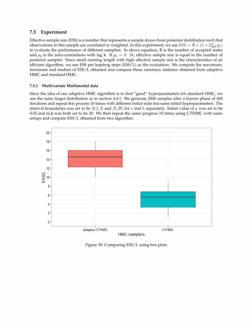
Since the idea of our adaptive HMC algorithm is to find ”good” hyperparameters for standard HMC, weuse the same target distribution as in section 4.4.1. We generate 2000 samples after a burnin phase of 400iterations and repeat this process 10 times with different initial state but same initial hyperparameters. Theinterval boundaries was set to be [0.1, 3] and [5, 25] for ε and L separately. Initial value of α was set to be0.02 and m,k was both set to be 20. We then repeat the same progress 10 times using CTHMC with samesetups and compare ESS/L obtained from two algorithm.

Figure 30: Comparing ESS/L using box plots

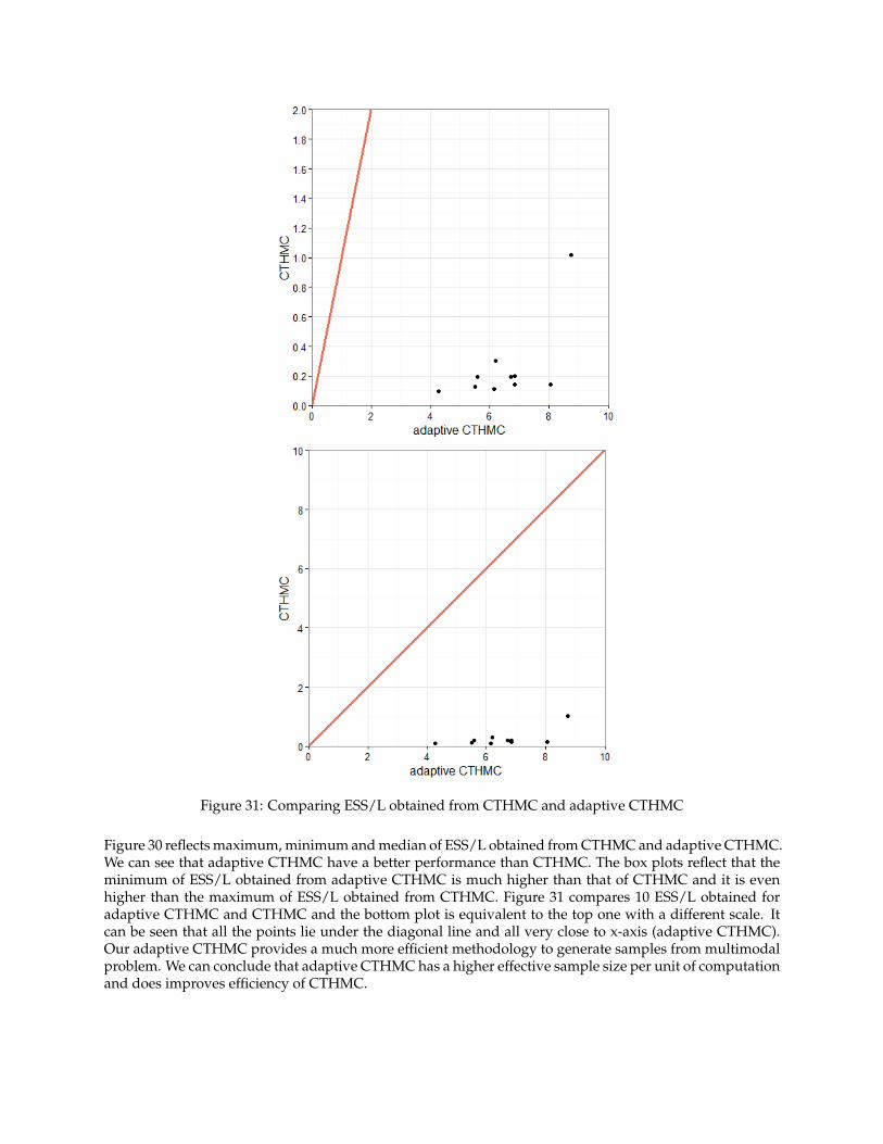
Figure 31: Comparing ESS/L obtained from CTHMC and adaptive CTHMC

Figure 30 reflects maximum, minimum and median of ESS/L obtained from CTHMC and adaptive CTHMC.We can see that adaptive CTHMC have a better performance than CTHMC. The box plots reflect that theminimum of ESS/L obtained from adaptive CTHMC is much higher than that of CTHMC and it is evenhigher than the maximum of ESS/L obtained from CTHMC. Figure 31 compares 10 ESS/L obtained foradaptive CTHMC and CTHMC and the bottom plot is equivalent to the top one with a different scale. Itcan be seen that all the points lie under the diagonal line and all very close to x-axis (adaptive CTHMC).Our adaptive CTHMC provides a much more efficient methodology to generate samples from multimodalproblem. We can conclude that adaptive CTHMC has a higher effective sample size per unit of computationand does improves efficiency of CTHMC.

7.6 Challenges

Although adaptive CTHMC also has its own problems. The performance of this algorithm is highly dependon the computation ability of the programming language. For example, this experiment is writing in Rprogramming language and R will recognize a parameter as INF if its value is too large (i.e. a = INF ifa > 1031). There is a high probability that βi+1 has a large value after several iterations depends on theinitial choice of δ. The algorithm will stop to find the ”better” hyperparameters if a parameter with INFappears. In addition, the dimension of K matrix will increasingly large with more iterations. Thus, time-cost will be high if larger samples are generated. Also, the goal of this algorithm is to tunning standardHMC; so, ti is better to make sure that standard HMC is able to generate expected samples from the targetdistribution with some initial choice of hyperparameters.

References

[1] Radford M.Neal**.MCMC Using Hamiltonian Dynamics--Chapter 5 of the Handbook of Markov ChainMonte Carlo, 2011

[2] Radford M.Neal**.The Short-Cut Metropolis Method, 2005

[3] Matthew M. Graham and Amos J, Storkey**.Continuously tempered Hamiltonian Monte Carlo, 2017

[4] Michael Betancourt**.A General Metric for Riemannian Manifolds Hamiltonian Monte Carlo, 2013

[5] Leimkuhler. B. and Reich. S**.Simulating Hamiltonian Dynamics--Cambridge University Press, 2004

[6] Michael Betancourt**.Hamiltonian Monte Carlo for Hierarchical Model, 2013

[7] Michael Betancourt**.A Conceptual Introduction to Hamiltonian Monte Carlo, 2017

[8] Ziyu Wang, Shakir Mohamed and Nando de Freitas**.Adaptive Hamiltonian and Riemann Manifold Monte Carlo Samplers, 2013

[9] Akihiko Nishimura and David B. Dunson**Geometrically Tempered Hamiltonian Monte Carlo, 2017

.