1

Harmonized Landsat-8 Sentinel-2 (HLS) Product User's Guide

Web site: http://hls.gsfc.nasa.gov/

Authors: Martin Claverie Jeffrey G. Masek Junchang Ju mcl@umd.edu jeffrey.g.masek@nasa.gov junchang.ju@nasa.gov

Product Version: 1.2

Document Version: 1.2

Release date: February 28th, 2016

2

Table of Contents 1 Introduction .......................................................................................................................................... 3

2 Products overview ................................................................................................................................ 3

2.1 HLS processing flowchart .............................................................................................................. 3

2.2 Products specifications ................................................................................................................. 3

2.3 Spectral bands ............................................................................................................................... 4

2.4 Output Projection and Gridding .................................................................................................... 4

3 Algorithms description .......................................................................................................................... 5

3.1 Spatial co-registration of input data ............................................................................................. 5

3.2 Atmospheric correction ................................................................................................................ 5

3.3 Cloud mask related masks ............................................................................................................ 5

3.4 View and illumination angles adjustment .................................................................................... 6

3.5 Bandpass adjustment .................................................................................................................... 7

3.6 Spatial resampling ......................................................................................................................... 8

4 Selected regions .................................................................................................................................... 9

5 Products formats ................................................................................................................................. 10

5.1 Files format ................................................................................................................................. 10

5.2 S10 ............................................................................................................................................... 10

5.3 S30 ............................................................................................................................................... 11

5.4 L30 ............................................................................................................................................... 11

5.5 Quality Assessment layers .......................................................................................................... 12

5.6 Metadata dictionary ................................................................................................................... 12

5.7 File naming .................................................................................................................................. 13

5.8 Products access and directories structure .................................................................................. 14

6 Quality Assessment ............................................................................................................................. 14

7 Known issues ....................................................................................................................................... 16

8 References .......................................................................................................................................... 16

3

1 Introduction

The combination of Landsat and Sentinel-2 data offers a unique opportunity to observe globally the land every 2-3 days at medium (<30m) spatial resolution. The Harmonized Landsat-Sentinel-2 (HLS) project is a NASA initiative to produce a consistent, harmonized surface reflectance product from Landsat and Sentinel-2 data.

In this context a “harmonized” reflectance product means that necessary radiometric, spectral, geometric, and spatial corrections have been applied to create a seamless time series, such that it is transparent to the user which sensor contributed any particular observation. It is also desirable that the harmonized products share a common gridding & tiling system, such that they are “stackable”.

Note: current HLS products (as of June 2016) are preliminary and unvalidated.

2 Products overview

2.1 HLS processing flowchart

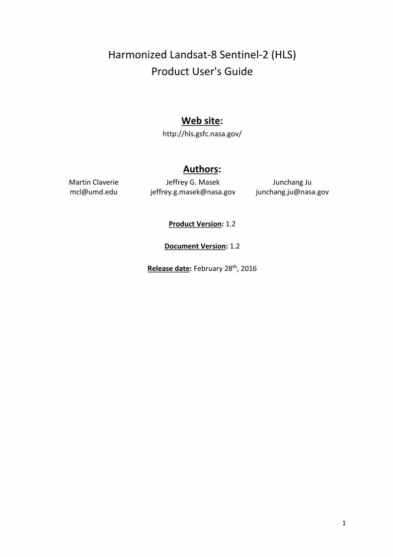
The processing (Figure 1) starts with orthorectified TOA reflectance data from Sentinel-2 (L1C) and Landsat-8 (L1T) and yields to three products: S10, S30 and L30.

Figure 1: HLS science algorithm processing flow

2.2 Products specifications

The HLS suite contains three products:

− S10: MSI surface reflectance at full (native) resolutions (i.e. 10m, 20m and 60m). − S30: MSI harmonized surface reflectance resampled to 30m using the Sentinel-2 MGRS tiling

system.

4

− L30: OLI harmonized surface reflectance and TOA brightness temperature resampled to 30m using the Sentinel-2 MGRS tiling system.

Note that the S30 and L30 products are gridded to the same resolution and tiling system, and thus are “stackable” for time series analysis.

Standard specifications are given in the Table 1.

Table 1: Products specifications

Product Name S10 S30 L30 Input sensor Sentinel-2A/B MSI Sentinel-2A/B MSI Landsat-8 OLI/TIRS Spatial resolution 10-20-60m 30m 30m BRDF-adjusted No Yes (except for bands

01, 05, 06, 07, 09, 10) Yes

Bandpass-adjusted No OLI-like No Projection UTM UTM UTM Tiling system MGRS (110*110) MGRS (110*110) MGRS (110*110)

2.3 Spectral bands

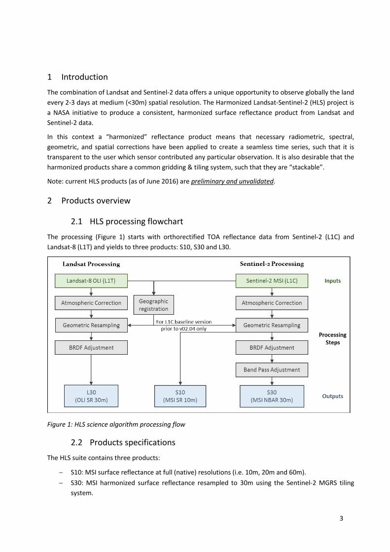
All Landsat-8 OLI and Sentinel-2 MSI reflective spectral bands are retained in the HLS products. Band 10 of Landsat-8 TIRS is reported in the L30, while band 11 is not because it is highly affected by a known stray light issue. HLS band numbers and code names are given in the Table 2.

Table 2: HLS spectral bands

Band name OLI band number

MSI band number

HLS band code name

Wavelength (micrometers)

Coastal Aerosol 1 1 CA 0.43 - 0.45* Blue 2 2 BLUE 0.45 - 0.51*

Green 3 3 GREEN 0.53 - 0.59* Red 4 4 RED 0.64 - 0.67*

Red-Edge 1 - 5 RE1 0.69-0.71** Red-Edge 2 - 6 RE2 0.73-0.75** Red-Edge 3 - 7 RE3 0.77-0.79** NIR Narrow 5 8A NIR1 0.85 - 0.88* NIR Broad - 8 NIR2 0.78-0.88**

SWIR 1 6 11 SWIR1 1.57 - 1.65* SWIR 2 7 12 SWIR2 2.11 - 2.29*

Water vapor - 9 WV 0.93-0.95** Cirrus 9 10 CIRRUS 1.36 - 1.38*

Thermal Infrared 1 10 - TIRS1 10.60 - 11.19*

* from OLI specifications (may vary for S10 product which follow MSI specifications); ** from MSI specifications

2.4 Output Projection and Gridding

The HLS tiling system is identical to the one used for Sentinel-2. Tiles use the UTM projection, and are 109,800m on a side. There is an overlap of 4,900m on each side for adjacent tiles of the same UTM zone. The tiling system is aligned with the Military Grid Reference System (MGRS) and its naming

5

convention derived from the UTM (Universal Transverse Mercator) system. The UTM system divides the Earth’s surface into 60 vertical zones. Each UTM zone has a horizontal width of 6° of longitude and vertical width of 8° of latitude, as shown in the map below. Each UTM zone is subdivided in 100x100km tiles. The first 2 digits in a tile name correspond to the UTM zone, the following 1 letter corresponds a 8° latitude band, and the two last letters to the tile location in the longitudinal and latitudinal directions respectively.

The kml edited by ESA with all tiles ID can be downloaded here. A text file with geographic coordinates of all tiles ID can be downloaded here.

3 Algorithms description

3.1 Spatial co-registration of input data

Landsat-8 and Sentinel-2 data have been found to not be accurately co-registered, due to small errors in the Landsat-8 ground reference system. Sentinel-2 L1C data with baseline processing version prior to v02.04 (v02.00, v02.01, v02.02) have also been found to not be accurately co-registered, affecting mostly cross-orbit temporal registration.

The Automated Registration and Orthorectification Package (AROP) for Landsat (Gao et al. 2009) was adapted for Sentinel-2 data processing, and is used to warp and co-register an image to a base image. Based on a large number of control points derived from cross-correlation of small areas, the package yields to the fit of a 1 degree polynomial equations system (eq. 1). This system is then used when applying the spatial resampling (section 3.6).

�𝑥𝑥′ = 𝑎𝑎1 + 𝑎𝑎2𝑥𝑥 + 𝑎𝑎3𝑦𝑦𝑦𝑦′ = 𝑏𝑏1 + 𝑏𝑏2𝑥𝑥 + 𝑏𝑏3𝑦𝑦

(1)

Where (x,y) and (x',y') correspond to the coordinates of the original and the warped image, respectively, and a1,2,3 and b1,2,3 the AROP coefficients.

The NIR band (B5 for OLI and B8A for MSI) is used for the cross-correlation analysis. The base (reference) image is defined by the less cloudy Sentinel-2 data selected among the data with baseline processing version v02.04 and a spatial coverage higher than 70% of the tile. A unique image is selected per tile using data acquired prior December 31st, 2016.

The warped image corresponds to all Landsat-8 data and Sentinel-2 tiles with baseline processing version prior to v02.04.

3.2 Atmospheric correction

The atmospheric correction method is based on continuous ratio map algorithm developed by Eric Vermote (NASA GSFC). A full description of the algorithm and the evaluation and validation of Landsat-8 OLI surface reflectance product is presented in (Vermote et al. 2016).

3.3 Cloud mask related masks

Landsat-8 cloud, cloud-shadow, snow and water masks are derived from the atmospheric tool introduced in 3.2.

6

Sentinel-2 cloud, cloud-shadow, snow and water mask relies on the Fmask algorithm which has been adapted from (Zhu et al. 2015). Fmask is run on 20m-aggregated TOA reflectance.

3.4 View and illumination angles adjustment

The S30 and L30 reflectance products are adjusted for the view and illumination angles. A view angle is set to nadir and the illumination is set constant per tile depending on the latitude.

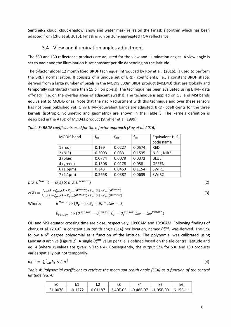
The c-factor global 12 month fixed BRDF technique, introduced by Roy et al. (2016), is used to perform the BRDF normalization. It consists of a unique set of BRDF coefficients, i.e., a constant BRDF shape, derived from a large number of pixels in the MODIS 500m BRDF product (MCD43) that are globally and temporally distributed (more than 15 billion pixels). The technique has been evaluated using ETM+ data off-nadir (i.e. on the overlap areas of adjacent swaths). The technique is applied on OLI and MSI bands equivalent to MODIS ones. Note that the nadir-adjustment with this technique and over these sensors has not been published yet. Only ETM+ equivalent bands are adjusted. BRDF coefficients for the three kernels (isotropic, volumetric and geometric) are shown in the Table 3. The kernels definition is described in the ATBD of MOD43 product (Strahler et al. 1999).

Table 3: BRDF coefficients used for the c-factor approach (Roy et al. 2016)

MODIS band fiso fgeo fvol Equivalent HLS code name

1 (red) 0.169 0.0227 0.0574 RED 2 (NIR) 0.3093 0.033 0.1535 NIR1, NIR2 3 (blue) 0.0774 0.0079 0.0372 BLUE 4 (green) 0.1306 0.0178 0.058 GREEN 6 (1.6μm) 0.343 0.0453 0.1154 SWIR1 7 (2.1μm) 0.2658 0.0387 0.0639 SWIR2

𝜌𝜌(𝜆𝜆,𝜃𝜃𝑁𝑁𝑁𝑁𝑁𝑁𝑁𝑁) = 𝑐𝑐(𝜆𝜆) × 𝜌𝜌(𝜆𝜆,𝜃𝜃𝑠𝑠𝑠𝑠𝑠𝑠𝑠𝑠𝑁𝑁𝑁𝑁) (2)

𝑐𝑐(𝜆𝜆) = 𝑓𝑓𝑖𝑖𝑖𝑖𝑖𝑖(𝜆𝜆)+𝑓𝑓𝑔𝑔𝑔𝑔𝑖𝑖(𝜆𝜆)×𝐾𝐾𝑔𝑔𝑔𝑔𝑖𝑖�𝜃𝜃𝑁𝑁𝑖𝑖𝑁𝑁𝑁𝑁�+𝑓𝑓𝑣𝑣𝑖𝑖𝑣𝑣(𝜆𝜆)×𝐾𝐾𝑣𝑣𝑖𝑖𝑣𝑣�𝜃𝜃𝑁𝑁𝑖𝑖𝑁𝑁𝑁𝑁�𝑓𝑓𝑖𝑖𝑖𝑖𝑖𝑖(𝜆𝜆)+𝑓𝑓𝑔𝑔𝑔𝑔𝑖𝑖(𝜆𝜆)×𝐾𝐾𝑔𝑔𝑔𝑔𝑖𝑖(𝜃𝜃𝑖𝑖𝑔𝑔𝑠𝑠𝑖𝑖𝑖𝑖𝑁𝑁)+𝑓𝑓𝑣𝑣𝑖𝑖𝑣𝑣(𝜆𝜆)×𝐾𝐾𝑣𝑣𝑖𝑖𝑣𝑣(𝜃𝜃𝑖𝑖𝑔𝑔𝑠𝑠𝑖𝑖𝑖𝑖𝑁𝑁) (3)

Where: 𝜃𝜃𝑁𝑁𝑁𝑁𝑁𝑁𝑁𝑁 ⇔ (𝜃𝜃𝑣𝑣 = 0,𝜃𝜃𝑠𝑠 = 𝜃𝜃𝑠𝑠𝑁𝑁𝑜𝑜𝑜𝑜,∆𝜑𝜑 = 0)

𝜃𝜃𝑠𝑠𝑠𝑠𝑠𝑠𝑠𝑠𝑁𝑁𝑁𝑁 ⇔ (𝜃𝜃𝑠𝑠𝑠𝑠𝑠𝑠𝑠𝑠𝑁𝑁𝑁𝑁 = 𝜃𝜃𝑣𝑣𝑠𝑠𝑠𝑠𝑠𝑠𝑠𝑠𝑁𝑁𝑁𝑁,𝜃𝜃𝑠𝑠 = 𝜃𝜃𝑠𝑠𝑠𝑠𝑠𝑠𝑠𝑠𝑠𝑠𝑁𝑁𝑁𝑁,∆𝜑𝜑 = ∆𝜑𝜑𝑠𝑠𝑠𝑠𝑠𝑠𝑠𝑠𝑁𝑁𝑁𝑁)

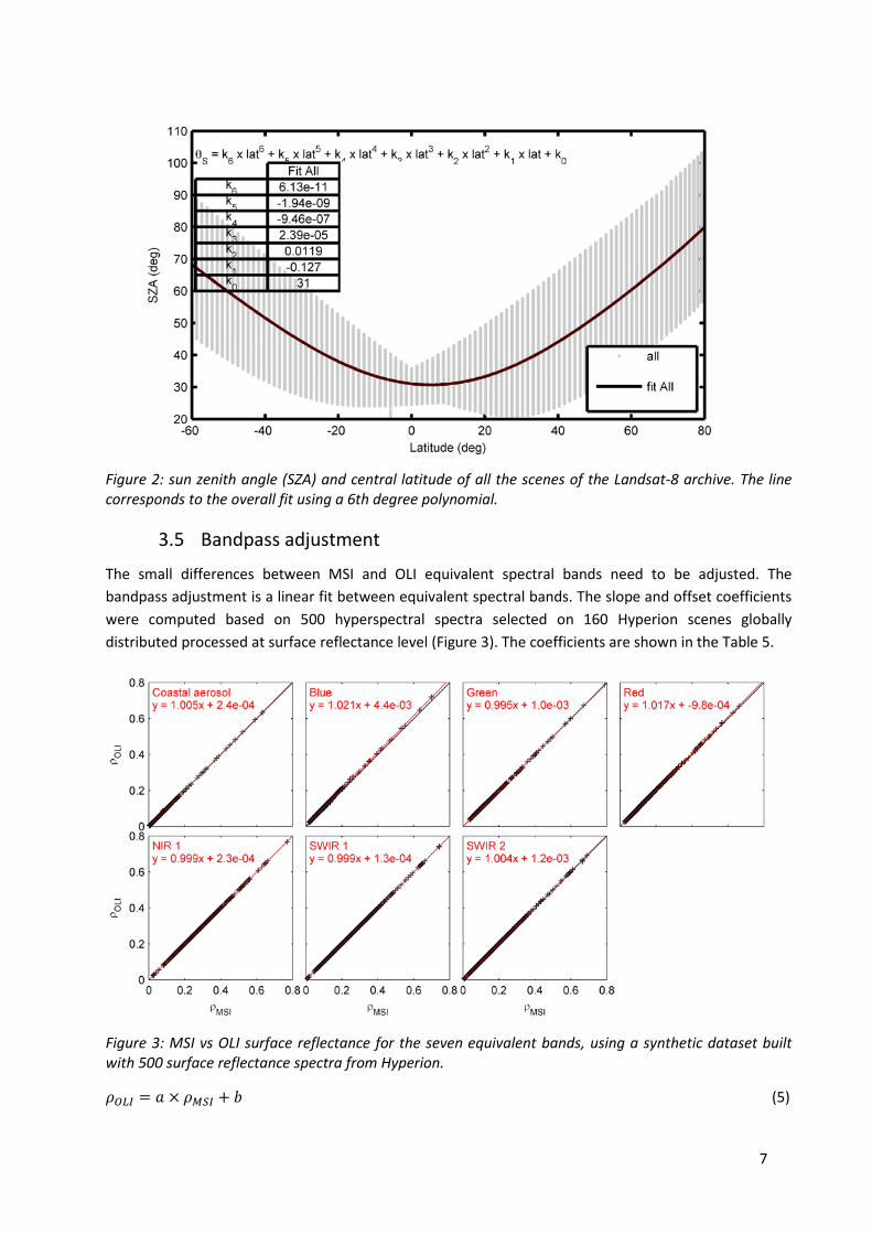
OLI and MSI equator crossing time are close, respectively, 10:00AM and 10:30AM. Following findings of Zhang et al. (2016), a constant sun zenith angle (SZA) per location, named 𝜃𝜃𝑠𝑠𝑁𝑁𝑜𝑜𝑜𝑜, was derived. The SZA follow a 6th degree polynomial as a function of the latitude. The polynomial was calibrated using Landsat-8 archive (Figure 2). A single 𝜃𝜃𝑠𝑠𝑁𝑁𝑜𝑜𝑜𝑜 value per tile is defined based on the tile central latitude and eq. 4 (where ki values are given in Table 4). Consequently, the output SZA for S30 and L30 products varies spatially but not temporally.

𝜃𝜃𝑠𝑠𝑁𝑁𝑜𝑜𝑜𝑜 = ∑ 𝑘𝑘𝑖𝑖 × 𝐿𝐿𝑎𝑎𝐿𝐿𝑖𝑖6𝑖𝑖=0 (4)

Table 4: Polynomial coefficient to retrieve the mean sun zenith angle (SZA) as a function of the central latitude (eq. 4)

k0 k1 k2 k3 k4 k5 k6 31.0076 -0.1272 0.01187 2.40E-05 -9.48E-07 -1.95E-09 6.15E-11

7

Figure 2: sun zenith angle (SZA) and central latitude of all the scenes of the Landsat-8 archive. The line corresponds to the overall fit using a 6th degree polynomial.

3.5 Bandpass adjustment

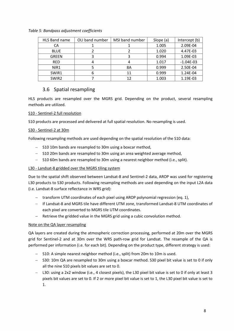
The small differences between MSI and OLI equivalent spectral bands need to be adjusted. The bandpass adjustment is a linear fit between equivalent spectral bands. The slope and offset coefficients were computed based on 500 hyperspectral spectra selected on 160 Hyperion scenes globally distributed processed at surface reflectance level (Figure 3). The coefficients are shown in the Table 5.

Figure 3: MSI vs OLI surface reflectance for the seven equivalent bands, using a synthetic dataset built with 500 surface reflectance spectra from Hyperion.

𝜌𝜌𝑂𝑂𝑂𝑂𝑂𝑂 = 𝑎𝑎 × 𝜌𝜌𝑀𝑀𝑀𝑀𝑂𝑂 + 𝑏𝑏 (5)

8

Table 5: Bandpass adjustment coefficients

HLS Band name OLI band number MSI band number Slope (a) Intercept (b) CA 1 1 1.005 2.09E-04

BLUE 2 2 1.020 4.47E-03 GREEN 3 3 0.994 1.09E-03

RED 4 4 1.017 -1.04E-03 NIR1 5 8A 0.999 2.50E-04

SWIR1 6 11 0.999 1.24E-04 SWIR2 7 12 1.003 1.19E-03

3.6 Spatial resampling

HLS products are resampled over the MGRS grid. Depending on the product, several resampling methods are utilized.

S10 - Sentinel-2 full resolution

S10 products are processed and delivered at full spatial resolution. No resampling is used.

S30 - Sentinel-2 at 30m

Following resampling methods are used depending on the spatial resolution of the S10 data:

− S10 10m bands are resampled to 30m using a boxcar method, − S10 20m bands are resampled to 30m using an area weighted average method, − S10 60m bands are resampled to 30m using a nearest neighbor method (i.e., split).

L30 - Landsat-8 gridded over the MGRS tiling system

Due to the spatial shift observed between Landsat-8 and Sentinel-2 data, AROP was used for registering L30 products to S30 products. Following resampling methods are used depending on the input L2A data (i.e. Landsat-8 surface reflectance in WRS grid):

− transform UTM coordinates of each pixel using AROP polynomial regression (eq. 1), − If Landsat-8 and MGRS tile have different UTM zone, transformed Landsat-8 UTM coordinates of

each pixel are converted to MGRS tile UTM coordinates. − Retrieve the gridded value in the MGRS grid using a cubic convolution method.

Note on the QA layer resampling

QA layers are created during the atmospheric correction processing, performed at 20m over the MGRS grid for Sentinel-2 and at 30m over the WRS path-row grid for Landsat. The resample of the QA is performed per information (i.e. for each bit). Depending on the product type, different strategy is used:

− S10: A simple nearest neighbor method (i.e., split) from 20m to 10m is used. − S30: 10m QA are resampled to 30m using a boxcar method. S30 pixel bit value is set to 0 if only

all the nine S10 pixels bit values are set to 0. − L30: using a 2x2 window (i.e., 4 closest pixels), the L30 pixel bit value is set to 0 if only at least 3

pixels bit values are set to 0. If 2 or more pixel bit value is set to 1, the L30 pixel bit value is set to 1.

9

4 Selected regions

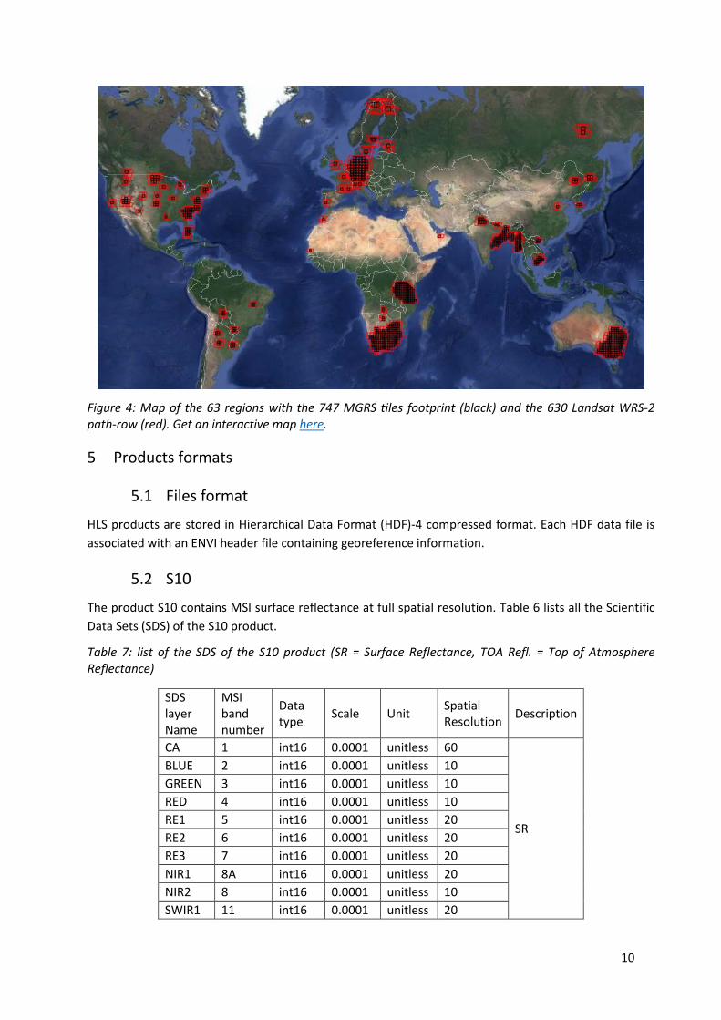
Sixty-three regions (Figure 4) were selected, corresponding to a total of 747 MGRS tiles. These tiles overlap with a total of 630 Landsat WRS-2 path-row. The list of the regions and the corresponding MGRS tiles can be downloaded here.

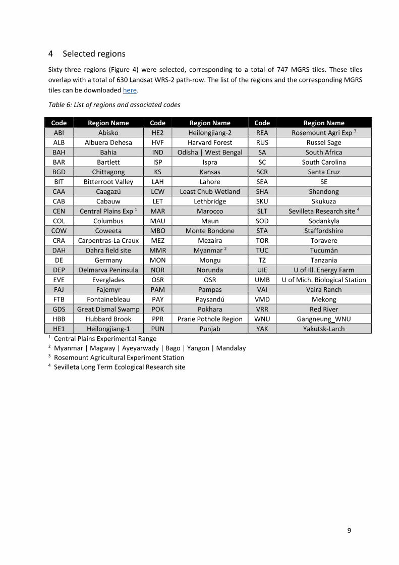
Table 6: List of regions and associated codes

Code Region Name Code Region Name Code Region Name ABI Abisko HE2 Heilongjiang-2 REA Rosemount Agri Exp 3 ALB Albuera Dehesa HVF Harvard Forest RUS Russel Sage BAH Bahia IND Odisha | West Bengal SA South Africa BAR Bartlett ISP Ispra SC South Carolina BGD Chittagong KS Kansas SCR Santa Cruz BIT Bitterroot Valley LAH Lahore SEA SE CAA Caagazú LCW Least Chub Wetland SHA Shandong CAB Cabauw LET Lethbridge SKU Skukuza CEN Central Plains Exp 1 MAR Marocco SLT Sevilleta Research site 4 COL Columbus MAU Maun SOD Sodankyla

COW Coweeta MBO Monte Bondone STA Staffordshire CRA Carpentras-La Craux MEZ Mezaira TOR Toravere DAH Dahra field site MMR Myanmar 2 TUC Tucumán DE Germany MON Mongu TZ Tanzania

DEP Delmarva Peninsula NOR Norunda UIE U of Ill. Energy Farm EVE Everglades OSR OSR UMB U of Mich. Biological Station FAJ Fajemyr PAM Pampas VAI Vaira Ranch FTB Fontainebleau PAY Paysandú VMD Mekong GDS Great Dismal Swamp POK Pokhara VRR Red River HBB Hubbard Brook PPR Prarie Pothole Region WNU Gangneung_WNU HE1 Heilongjiang-1 PUN Punjab YAK Yakutsk-Larch

1 Central Plains Experimental Range 2 Myanmar | Magway | Ayeyarwady | Bago | Yangon | Mandalay 3 Rosemount Agricultural Experiment Station 4 Sevilleta Long Term Ecological Research site

10

Figure 4: Map of the 63 regions with the 747 MGRS tiles footprint (black) and the 630 Landsat WRS-2 path-row (red). Get an interactive map here.

5 Products formats

5.1 Files format

HLS products are stored in Hierarchical Data Format (HDF)-4 compressed format. Each HDF data file is associated with an ENVI header file containing georeference information.

5.2 S10

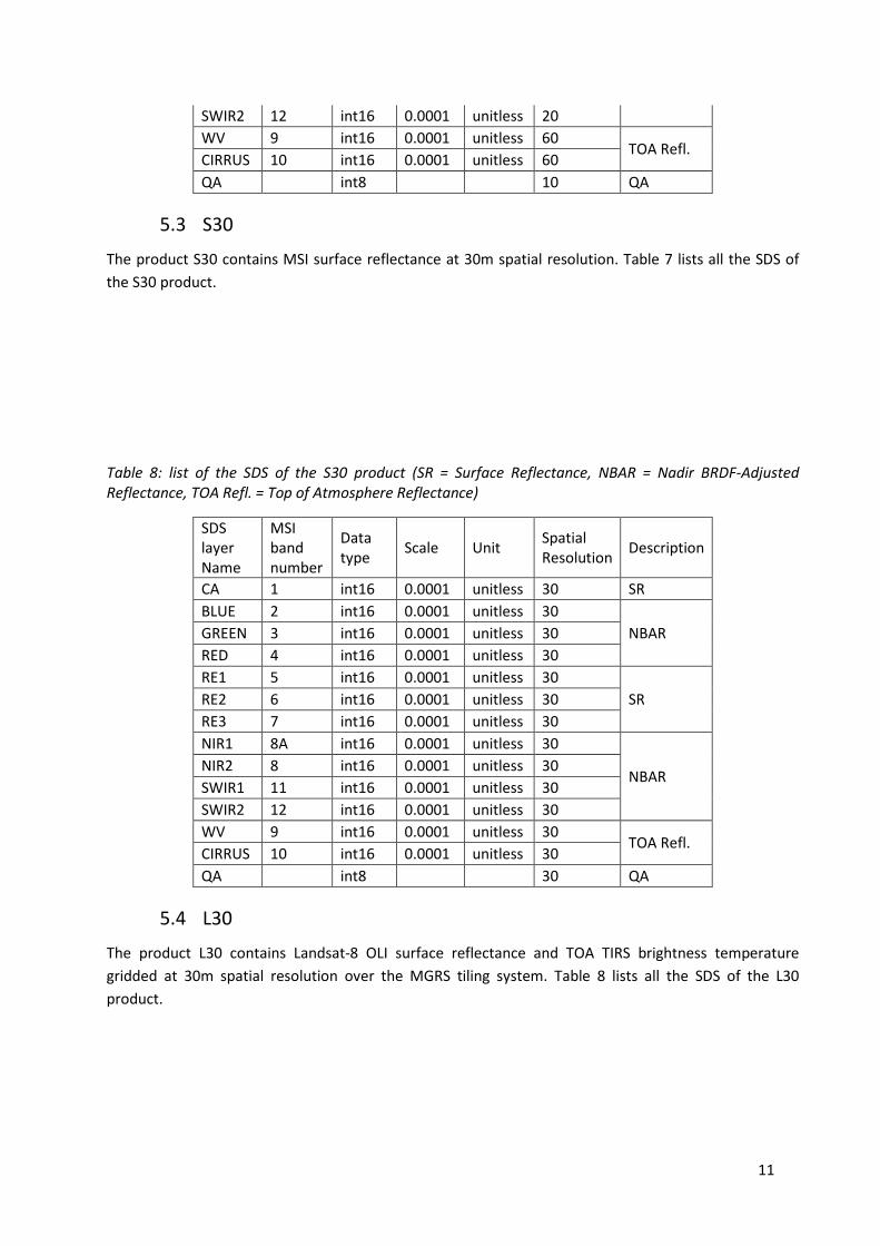
The product S10 contains MSI surface reflectance at full spatial resolution. Table 6 lists all the Scientific Data Sets (SDS) of the S10 product.

Table 7: list of the SDS of the S10 product (SR = Surface Reflectance, TOA Refl. = Top of Atmosphere Reflectance)

SDS layer Name

MSI band number

Data type Scale Unit Spatial

Resolution Description

CA 1 int16 0.0001 unitless 60

SR

BLUE 2 int16 0.0001 unitless 10 GREEN 3 int16 0.0001 unitless 10 RED 4 int16 0.0001 unitless 10 RE1 5 int16 0.0001 unitless 20 RE2 6 int16 0.0001 unitless 20 RE3 7 int16 0.0001 unitless 20 NIR1 8A int16 0.0001 unitless 20 NIR2 8 int16 0.0001 unitless 10 SWIR1 11 int16 0.0001 unitless 20

11

SWIR2 12 int16 0.0001 unitless 20 WV 9 int16 0.0001 unitless 60

TOA Refl. CIRRUS 10 int16 0.0001 unitless 60 QA int8 10 QA

5.3 S30

The product S30 contains MSI surface reflectance at 30m spatial resolution. Table 7 lists all the SDS of the S30 product.

Table 8: list of the SDS of the S30 product (SR = Surface Reflectance, NBAR = Nadir BRDF-Adjusted Reflectance, TOA Refl. = Top of Atmosphere Reflectance)

SDS layer Name

MSI band number

Data type Scale Unit Spatial

Resolution Description

CA 1 int16 0.0001 unitless 30 SR BLUE 2 int16 0.0001 unitless 30

NBAR GREEN 3 int16 0.0001 unitless 30 RED 4 int16 0.0001 unitless 30 RE1 5 int16 0.0001 unitless 30

SR RE2 6 int16 0.0001 unitless 30 RE3 7 int16 0.0001 unitless 30 NIR1 8A int16 0.0001 unitless 30

NBAR NIR2 8 int16 0.0001 unitless 30 SWIR1 11 int16 0.0001 unitless 30 SWIR2 12 int16 0.0001 unitless 30 WV 9 int16 0.0001 unitless 30

TOA Refl. CIRRUS 10 int16 0.0001 unitless 30 QA int8 30 QA

5.4 L30

The product L30 contains Landsat-8 OLI surface reflectance and TOA TIRS brightness temperature gridded at 30m spatial resolution over the MGRS tiling system. Table 8 lists all the SDS of the L30 product.

12

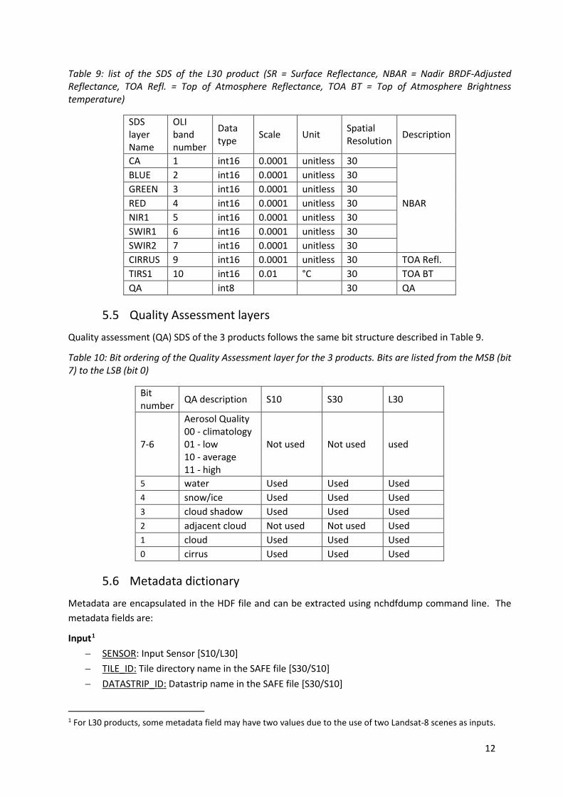
Table 9: list of the SDS of the L30 product (SR = Surface Reflectance, NBAR = Nadir BRDF-Adjusted Reflectance, TOA Refl. = Top of Atmosphere Reflectance, TOA BT = Top of Atmosphere Brightness temperature)

SDS layer Name

OLI band number

Data type Scale Unit Spatial

Resolution Description

CA 1 int16 0.0001 unitless 30

NBAR

BLUE 2 int16 0.0001 unitless 30 GREEN 3 int16 0.0001 unitless 30 RED 4 int16 0.0001 unitless 30 NIR1 5 int16 0.0001 unitless 30 SWIR1 6 int16 0.0001 unitless 30 SWIR2 7 int16 0.0001 unitless 30 CIRRUS 9 int16 0.0001 unitless 30 TOA Refl. TIRS1 10 int16 0.01 °C 30 TOA BT QA int8 30 QA

5.5 Quality Assessment layers

Quality assessment (QA) SDS of the 3 products follows the same bit structure described in Table 9.

Table 10: Bit ordering of the Quality Assessment layer for the 3 products. Bits are listed from the MSB (bit 7) to the LSB (bit 0)

Bit number QA description S10 S30 L30

7-6

Aerosol Quality 00 - climatology 01 - low 10 - average 11 - high

Not used Not used used

5 water Used Used Used 4 snow/ice Used Used Used 3 cloud shadow Used Used Used 2 adjacent cloud Not used Not used Used 1 cloud Used Used Used 0 cirrus Used Used Used

5.6 Metadata dictionary

Metadata are encapsulated in the HDF file and can be extracted using nchdfdump command line. The metadata fields are:

Input1 − SENSOR: Input Sensor [S10/L30] − TILE_ID: Tile directory name in the SAFE file [S30/S10] − DATASTRIP_ID: Datastrip name in the SAFE file [S30/S10]

1 For L30 products, some metadata field may have two values due to the use of two Landsat-8 scenes as inputs.

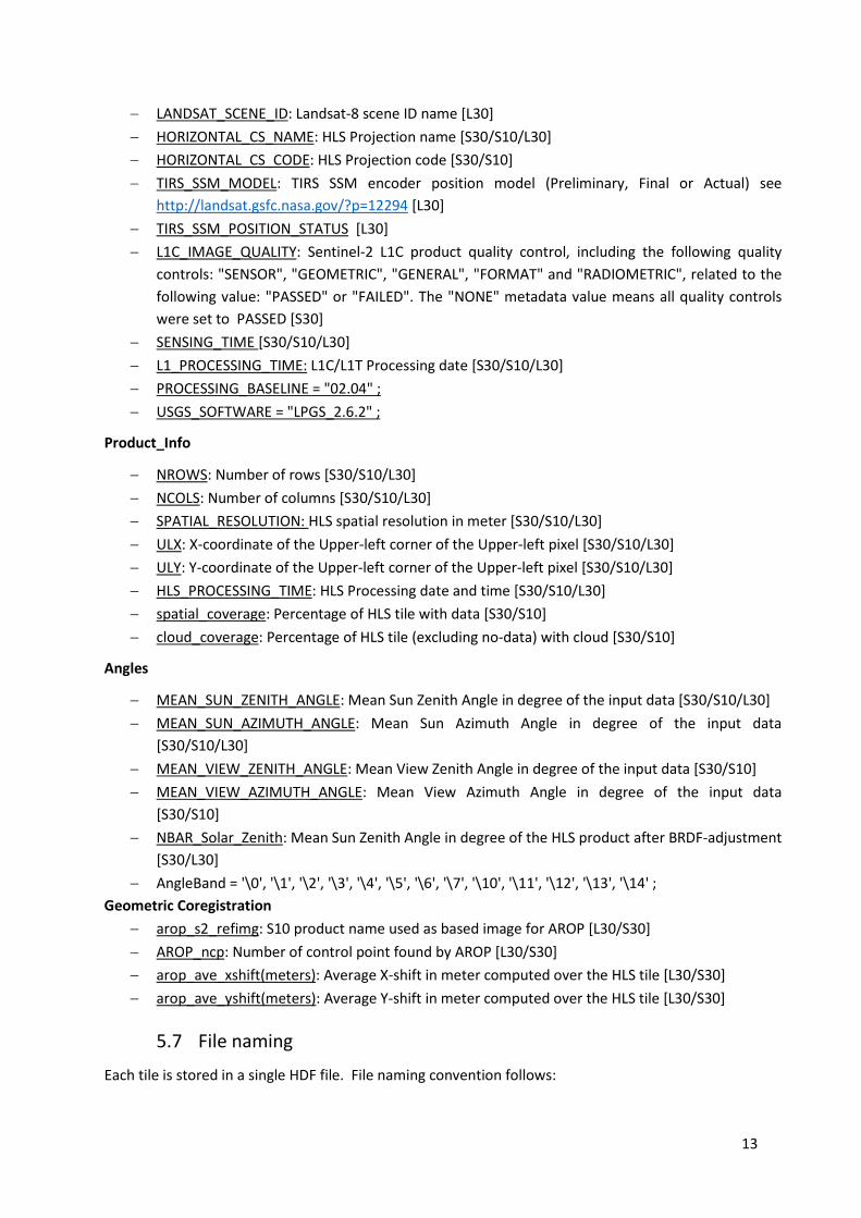
13

− LANDSAT_SCENE_ID: Landsat-8 scene ID name [L30] − HORIZONTAL_CS_NAME: HLS Projection name [S30/S10/L30] − HORIZONTAL_CS_CODE: HLS Projection code [S30/S10] − TIRS_SSM_MODEL: TIRS SSM encoder position model (Preliminary, Final or Actual) see

http://landsat.gsfc.nasa.gov/?p=12294 [L30] − TIRS_SSM_POSITION_STATUS [L30] − L1C_IMAGE_QUALITY: Sentinel-2 L1C product quality control, including the following quality

controls: "SENSOR", "GEOMETRIC", "GENERAL", "FORMAT" and "RADIOMETRIC", related to the following value: "PASSED" or "FAILED". The "NONE" metadata value means all quality controls were set to PASSED [S30]

− SENSING_TIME [S30/S10/L30] − L1_PROCESSING_TIME: L1C/L1T Processing date [S30/S10/L30] − PROCESSING_BASELINE = "02.04" ; − USGS_SOFTWARE = "LPGS_2.6.2" ;

Product_Info

− NROWS: Number of rows [S30/S10/L30] − NCOLS: Number of columns [S30/S10/L30] − SPATIAL_RESOLUTION: HLS spatial resolution in meter [S30/S10/L30] − ULX: X-coordinate of the Upper-left corner of the Upper-left pixel [S30/S10/L30] − ULY: Y-coordinate of the Upper-left corner of the Upper-left pixel [S30/S10/L30] − HLS_PROCESSING_TIME: HLS Processing date and time [S30/S10/L30] − spatial_coverage: Percentage of HLS tile with data [S30/S10] − cloud_coverage: Percentage of HLS tile (excluding no-data) with cloud [S30/S10]

Angles

− MEAN_SUN_ZENITH_ANGLE: Mean Sun Zenith Angle in degree of the input data [S30/S10/L30] − MEAN_SUN_AZIMUTH_ANGLE: Mean Sun Azimuth Angle in degree of the input data

[S30/S10/L30] − MEAN_VIEW_ZENITH_ANGLE: Mean View Zenith Angle in degree of the input data [S30/S10] − MEAN_VIEW_AZIMUTH_ANGLE: Mean View Azimuth Angle in degree of the input data

[S30/S10] − NBAR_Solar_Zenith: Mean Sun Zenith Angle in degree of the HLS product after BRDF-adjustment

[S30/L30] − AngleBand = '\0', '\1', '\2', '\3', '\4', '\5', '\6', '\7', '\10', '\11', '\12', '\13', '\14' ;

Geometric Coregistration − arop_s2_refimg: S10 product name used as based image for AROP [L30/S30] − AROP_ncp: Number of control point found by AROP [L30/S30] − arop_ave_xshift(meters): Average X-shift in meter computed over the HLS tile [L30/S30] − arop_ave_yshift(meters): Average Y-shift in meter computed over the HLS tile [L30/S30]

5.7 File naming

Each tile is stored in a single HDF file. File naming convention follows:

14

HLS.<HLS_Product>.T<Tile_ID>.<year><doy>.v<version_number>.hdf

Where,

− <HLS_Product> is the HLS product type (S10, S30 or L30) [3 digits] − <Tile_ID> is the MGRS Tile ID [5 digits] − <Year> is the sensing time year [4 digits] − <Doy> is the sensing time day of year [3 digits] − <Version_number> is the HLS version number (e.g., 1.2, major and minor changes reflected in

the first and second digits respectively) [3 digits]

5.8 Products access and directories structure

S10, S30 and L30 files are stored in the NASA NEX facility in the following directory:

/nobackuppp6/jju/HLS_LOCAL_IO.v1.2/

S30 and L30 files are also stored in a public FTP:

ftp://hls.gsfc.nasa.gov/pub/data/v1.2/

In both storage location, files are stored in a hierarchical directory structure designed as follow:

./<Region>/<HLS_Product>/<year>/<Tile_ID>/

Where,

− <Region> is the Region code as defined in Table 6 [2 or 3 digits] − <HLS_Product> is the HLS product type (S10, S30 or L30) [3 digits] − <Year> is the sensing time year [4 digits] − <Tile_ID> is the MGRS Tile ID [5 digits]

6 Quality Assessment

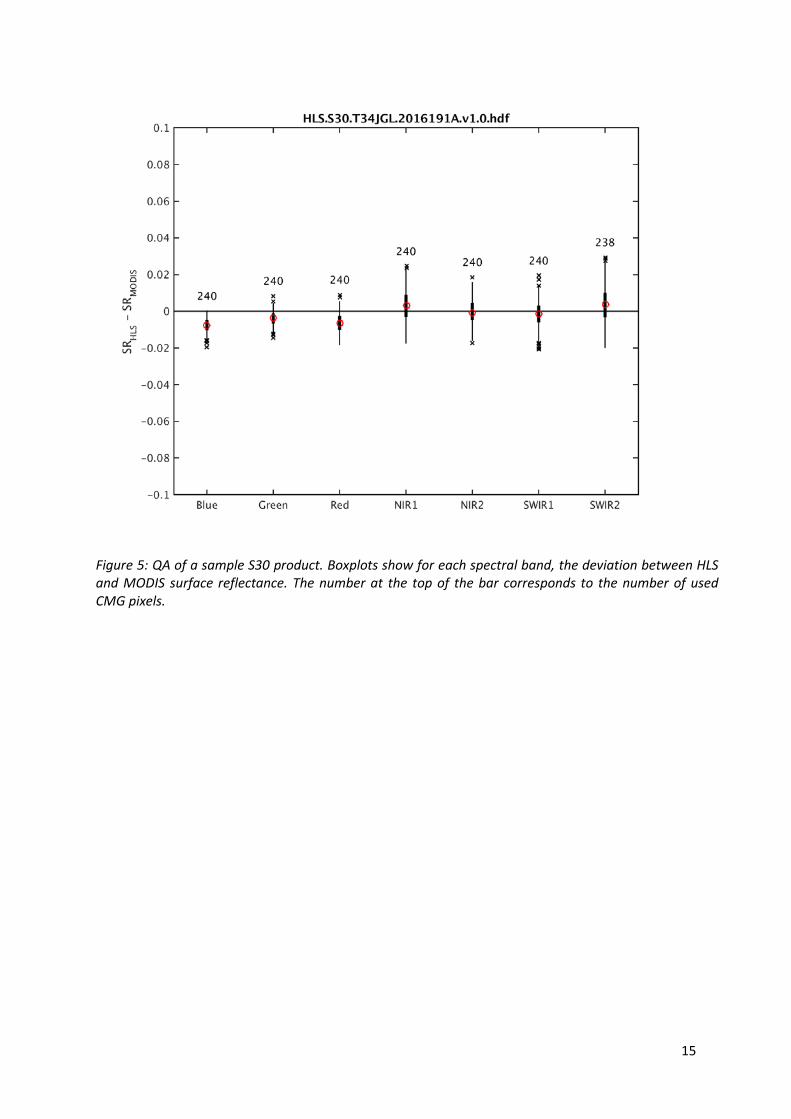
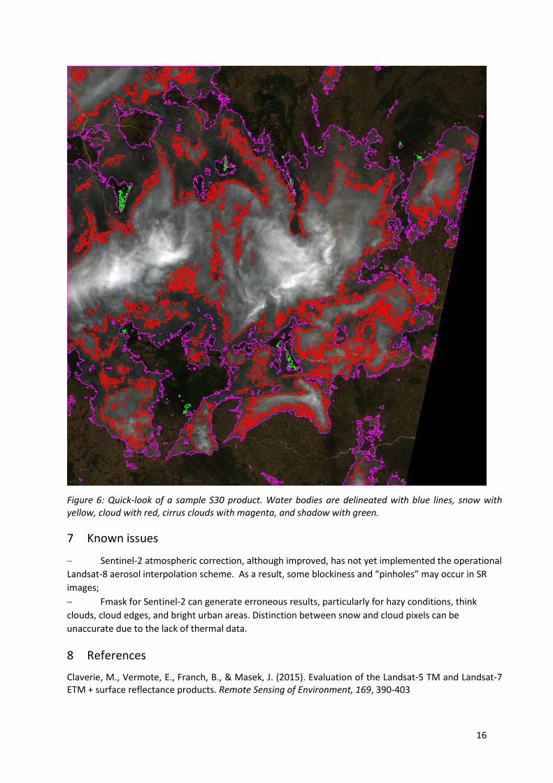
An evaluation of the S30 and L30 products has been applied. It follow the methodology of the cross-comparison of surface reflectance with MODIS MOD09CMG products involving BRDF and spectral adjustment (Claverie et al. 2015). The results are gathered in a table located here and individual QA graphics are linked in the table (Figure 5). Quick-look figures are also produced for each L30 and S30 products at 30m spatial resolution and at 120m spatial resolution (Figure 6).

15

Figure 5: QA of a sample S30 product. Boxplots show for each spectral band, the deviation between HLS and MODIS surface reflectance. The number at the top of the bar corresponds to the number of used CMG pixels.

16

Figure 6: Quick-look of a sample S30 product. Water bodies are delineated with blue lines, snow with yellow, cloud with red, cirrus clouds with magenta, and shadow with green.

7 Known issues

− Sentinel-2 atmospheric correction, although improved, has not yet implemented the operational Landsat-8 aerosol interpolation scheme. As a result, some blockiness and “pinholes” may occur in SR images; − Fmask for Sentinel-2 can generate erroneous results, particularly for hazy conditions, think clouds, cloud edges, and bright urban areas. Distinction between snow and cloud pixels can be unaccurate due to the lack of thermal data.

8 References

Claverie, M., Vermote, E., Franch, B., & Masek, J. (2015). Evaluation of the Landsat-5 TM and Landsat-7 ETM + surface reflectance products. Remote Sensing of Environment, 169, 390-403

17

Gao, F., Masek, J.G., & Wolfe, R.E. (2009). Automated registration and orthorectification package for Landsat and Landsat-like data processing. Journal of Applied Remote Sensing, 3

Roy, D.P., Zhang, H.K., Ju, J., Gomez-Dans, J.L., Lewis, P.E., Schaaf, C.B., Sun, Q., Li, J., Huang, H., & Kovalskyy, V. (2016). A general method to normalize Landsat reflectance data to nadir BRDF adjusted reflectance. Remote Sensing of Environment, 176, 255-271

Strahler, A.H., Lucht, W., Schaaf, C.B., Tsang, T., Gao, F., Li, X., Lewis, P., & Barnsley, M. (1999). MODIS BRDF/Albedo Product: Algorithm Theoretical Basis Document Version 5.0. In M. documentation (Ed.). Boston

Vermote, E., Justice, C., Claverie, M., & Franch, B. (2016). Preliminary analysis of the performance of the Landsat 8/OLI land surface reflectance product. Remote Sensing of Environment

Zhang, H.K., Roy, D.P., & Kovalskyy, V. (2016). Optimal Solar Geometry Definition for Global Long-Term Landsat Time-Series Bidirectional Reflectance Normalization. Ieee Transactions on Geoscience and Remote Sensing, 54, 1410-1418

Zhu, Z., Wang, S., & Woodcock, C.E. (2015). Improvement and expansion of the Fmask algorithm: cloud, cloud shadow, and snow detection for Landsats 4-7, 8, and Sentinel 2 images. Remote Sensing of Environment, 159, 269-277