Haskell High Performance Programming

Table of Contents

Haskell High Performance ProgrammingCreditsAbout the AuthorAbout the Reviewerwww.PacktPub.com

eBooks, discount offers, and moreWhy subscribe?

PrefaceWhat this book coversWhat you need for this bookWho this book is forConventionsReader feedbackCustomer support

Downloading the example codeDownloading the color images of this bookErrataPiracyQuestions

1. Identifying BottlenecksMeeting lazy evaluation

Writing sum correctlyWeak head normal formFolding correctly

Memoization and CAFsConstant applicative form

Recursion and accumulatorsThe worker/wrapper idiomGuarded recursionAccumulator parameters

Inspecting time and space usageIncreasing sharing and minimizing allocation

Compiler code optimizationsInlining and stream fusionPolymorphism performancePartial functions

Summary2. Choosing the Correct Data Structures

Annotating strictness and unpacking datatype fieldsUnbox with UNPACK

Using anonymous tuplesPerformance of GADTs and branching

Handling numerical data

Handling binary and textual dataRepresenting bit arraysHandling bytes and blobs of bytesWorking with characters and strings

Using the text libraryBuilders for iterative construction

Builders for stringsHandling sequential data

Using difference listsDifference list performanceDifference list with the Writer monad

Using zippersAccessing both ends fast with Seq

Handling tabular dataUsing the vector package

Handling sparse dataUsing the containers packageUsing the unordered-containers package

Ephemeral data structuresMutable references are slowUsing mutable arraysUsing mutable vectors

Bubble sort with vectorsWorking with monads and monad stacks

The list monad and its transformerFree monadsWorking with monad transformersSpeedup via continuation-passing style

Summary3. Profile and Benchmark to Your Heart's Content

Profiling time and allocationsSetting cost centres manuallySetting cost centres automaticallyInstalling libraries with profilingDebugging unexpected crashes with profiler

Heap profilingCost centre-based heap profilingObjects outside the heapRetainer profilingBiographical profiling

Benchmarking using the criterion libraryProfile and monitor in real time

Monitoring over HTTP with ekgSummary

4. The Devil's in the DetailThe anatomy of a Haskell project

Useful fields and flags in cabal filesTest suites and benchmarksUsing the stack toolMulti-package projects

Erroring and handling exceptionsHandling synchronous errorsThe exception hierarchyHandling asynchronous errorsThrow and catch in other monads besides IO

Writing tests for HaskellProperty checksUnit testing with HUnitTest frameworks

Trivia at term-levelCoding in GHC PrimOpsControl inlining

Using rewrite rulesSpecializing definitionsPhase control

Trivia at type-levelPhantom typesFunctional dependenciesType families and associated types

Useful GHC extensionsMonomorphism RestrictionExtensions for patterns and guardsStrict-by-default Haskell

Summary5. Parallelize for Performance

Primitive parallelism and the Runtime SystemSpark awaySubtle evaluation – pseqWhen in doubt, use the force

The Eval monad and strategiesComposing strategiesFine-tune granularity with chunking and buffering

The Par monad and schedulesspawn for futures and promisesNon-deterministic parallelism with ParIO

Diagnosing parallelism – ThreadScopeData parallel programming – Repa

Playing with Repa in GHCiMapping and delayed arraysReduction via folding

Manifest representationsDelayed representation and fusion

Indices, slicing, and extending arraysConvolution with stencilsCursored and partitioned arraysWriting fast Repa codeAdditional librariesExample from image processing

Loading the image from fileIdentifying letters with convolutionExtracting strings from an imageTesting and evaluating performance

Summary6. I/O and Streaming

Reading, writing, and handling resourcesTraps of lazy I/OFile handles, buffering, and encodingBinary I/OTextual I/OI/O performance with filesystem objectsSockets and networking

Acting as a TCP/IP clientActing as a TCP server (Unix domain sockets)Raw UDP trafficNetworking above the transport layer

Managing resources with ResourceTStreaming with side-effects

Choosing a streaming librarySimple streaming using io-streams

Creating input streamsUsing combinators and output streamsHandling exceptions and resources in streamsAn example of parsing using io-streams and attoparsec

Streaming using pipesComposing and executing pipesFor loops and category theory in pipesHandling exceptions in pipesStrengths and weaknesses of pipes

Streaming using conduitsHandling resources and exceptions in conduitsResuming conduits

Logging in HaskellLogging with FastLogger

More abstract loggersTimed log messagesMonadic logging

Customizing monadic loggersSummary

7. Concurrency and PerformanceThreads and concurrency primitives

Threads and mutable referencesAvoid accumulating thunksAtomic operations with IORefs

MVarMVars are fairMVar as a building block

Broadcasting with ChanSoftware Transactional Memory

STM example – Bank accountsAlternative transactionsExceptions in STM

Runtime System and threadsMasking asynchronous exceptions

Asynchronous processingUsing the Async API

Async example – TimeoutsComposing with Concurrently

Lifting up from I/OTop-level mutable referencesLifting from a base monadLifting base with exception handling

Summary8. Tweaking the Compiler and Runtime System (GHC)

Using GHC like a proOperating GHC

Circular dependenciesAdjusting optimizations and transformations

The state hackFloating lets in and outEliminating common subexpressionsLiberate-case duplicates code

Compiling via the LLVM routeLinking and building shared librariesPreprocessing Haskell source codeEnforcing type-safety using Safe Haskell

Tuning GHC's Runtime SystemScheduler and green threads

Sparks and spark poolBounded threads and affinityIndefinite blocking and weak references

Heap, stack, and memory managementEvaluation stack in Haskell

Tuning the garbage collectorParallel GC

Profiling and tracing optionsTracing using eventlogOptions for profiling and debugging

Summary of useful GHC optionsBasic usageThe LLVM backendTurn optimizations on and offConfiguring the Runtime System (compile-time)Safe Haskell

Summary of useful RTS optionsScheduler flagsMemory managementGarbage collectionRuntime System statisticsProfiling and debugging

Summary9. GHC Internals and Code Generation

Interpreting GHC's internal representationsReading GHC CoreSpineless tagless G-machine

Primitive GHC-specific featuresKinds encode type representation

Datatype generic programmingWorking example – A generic sum

Generating Haskell with HaskellSplicing with $(…)Names in templatesSmart template constructorsThe constN functionLifting Haskell code to Q with quotation bracketsLaunching missiles during compilationReifying Haskell data into template objectsDeriving setters with Template HaskellQuasi-quoting for DSLs

Summary10. Foreign Function Interface

From Haskell to C and C to HaskellCommon types in Haskell and CImporting static functions and addressesExporting Haskell functionsCompiling a shared libraryFunction pointers and wrappers

Haskell callbacks from CData marshal and stable pointers

Allocating memory outside the heapPointing to objects in the heap

Marshalling abstract datatypesMarshalling in standard libraries

Summary11. Programming for the GPU with Accelerate

Writing Accelerate programsKernels – The motivation behind explicit use and runWorking with elements and scalarsRudimentary array computationsExample – Matrix multiplicationFlow control and conditional executionInspecting generated code

Running with the CUDA backendDebugging CUDA programs

More Accelerate conceptsWorking with tuplesFolding, reducing, and segmentingAccelerated stencilsPermutations in AccelerateUsing the backend foreign function interface

Summary12. Scaling to the Cloud with Cloud Haskell

Processes and message-passingCreating a message typeCreating a ProcessSpawning and closuresRunning with the SimpleLocalNet backendUsing channelsEstablishing bidirectional channelsCalling a remote process

Handling failureFiring up monitorsMatching on the message queueLinking processes togetherMessage-passing performance

Nodes and networkingSummary

13. Functional Reactive ProgrammingThe tiny discrete-time Elerea

Mutually recursive signalsSignalling side-effectsDynamically changing signal networksPerformance and limitations in Elerea

Events and signal functions with YampaAdding state to signal functionsWorking with timeSwitching and discrete-time events

Integrating to the real worldReactive-banana – Safe and simple semantics

Example – First GUI applicationGraphical display with wxWidgets

Combining events and behaviorsSwitching events and behaviorsObserving moments on demandRecursion and semanticsAdding input and output

Input via polling or handlersReactimate outputInput and output dynamically

Summary14. Library Recommendations

Representing dataFunctional graphsNumeric data for special useEncoding and serialization

Binary serialization of Haskell valuesEncoding to and from other formatsCSV input and output

Persistent storage, SQL, and NoSQLacid-state and safecopypersistent and esqueletoHDBC and add-ons

Networking and HTTPHTTP clients and serversSupplementary HTTP librariesJSON remote procedure callsUsing WebSocketsProgramming a REST API

CryptographyWeb technologiesParsing and pretty-printing

Regular expressions in HaskellParsing XML

Pretty-printing and text formattingControl and utility libraries

Using lensesEasily converting between types (convertible)Using a custom Prelude

Working with monads and transformersMonad morphisms – monad-unlift

Handling exceptionsRandom number generatorsParallel and concurrent programming

Functional Reactive ProgrammingMathematics, statistics, and scienceTools for research and sketchingThe HaskellR projectCreating charts and diagramsScripting and CLI applicationsTesting and benchmarkingSummary

Index

Haskell High Performance Programming

Haskell High Performance ProgrammingCopyright © 2016 Packt Publishing

All rights reserved. No part of this book may be reproduced, stored in a retrieval system, or transmittedin any form or by any means, without the prior written permission of the publisher, except in the case ofbrief quotations embedded in critical articles or reviews.

Every effort has been made in the preparation of this book to ensure the accuracy of the informationpresented. However, the information contained in this book is sold without warranty, either express orimplied. Neither the author, nor Packt Publishing, and its dealers and distributors will be held liable forany damages caused or alleged to be caused directly or indirectly by this book.

Packt Publishing has endeavored to provide trademark information about all of the companies andproducts mentioned in this book by the appropriate use of capitals. However, Packt Publishing cannotguarantee the accuracy of this information.

First published: September 2016

Production reference: 1190916

Published by Packt Publishing Ltd.

Livery Place

35 Livery Street

Birmingham B3 2PB, UK.

ISBN 978-1-78646-421-7

www.packtpub.com

CreditsAuthor

Samuli Thomasson

Reviewer

Aaron Stevens

Commissioning Editor

Kunal Parikh

Acquisition Editor

Sonali Vernekar

Content Development Editor

Priyanka Mehta

Technical Editor

Ravikiran Pise

Copy Editor

Safis Editing

Project Coordinator

Izzat Contractor

Proofreader

Safis Editing

Indexer

Tejal Daruwale Soni

Graphics

Abhinash Sahu

Production Coordinator

Melwyn Dsa

Cover Work

Melwyn Dsa

About the AuthorSamuli Thomasson is a long-time functional programming enthusiast from Finland who has used Haskellextensively, both as a pastime and commercially, for over four years. He enjoys working with great toolsthat help in getting things done nice and fast.

His current job at RELEX Solutions consists of providing technical solutions to a variety of practicalproblems. Besides functional programming, Samuli is interested in distributed systems, which he alsostudies at the University of Helsinki.

I am grateful to my awesome friends, who have stuck around and provided their support during thewriting process, and my family for always being there and their understanding.

About the ReviewerAaron Stevens is a scientific software engineer with Molex LLC in Little Rock, Arkansas, where hecombines his passion for programming with his education in electrical systems engineering to developinnovative techniques to characterize high-speed electronics in the lab and in production. He specializesin signal processing, statistical process-control methods, and application construction in Python and C#,and he enjoys discovering new methods to explore complex data sets through rich visualizations.

Away from the office, Aaron enjoys practicing with a variety of programming languages, studyinglinguistics, cooking, and spending time with his family. He received his BS in mathematics and BS inelectrical systems engineering from the University of Arkansas in Little Rock.

www.PacktPub.com

eBooks, discount offers, and moreDid you know that Packt offers eBook versions of every book published, with PDF and ePub filesavailable? You can upgrade to the eBook version at www.PacktPub.com and as a print book customer,you are entitled to a discount on the eBook copy. Get in touch with us at<customercare@packtpub.com> for more details.

At www.PacktPub.com, you can also read a collection of free technical articles, sign up for a range offree newsletters and receive exclusive discounts and offers on Packt books and eBooks.

https://www2.packtpub.com/books/subscription/packtlib

Do you need instant solutions to your IT questions? PacktLib is Packt's online digital book library. Here,you can search, access, and read Packt's entire library of books.

Why subscribe?Fully searchable across every book published by PacktCopy and paste, print, and bookmark contentOn demand and accessible via a web browser

PrefaceHaskell is an elegant language. It allows us to express in code exactly what we mean, in a clean andcompact style. The nice features, including referential transparency and call-by-need evaluation, not onlyhelp the programmer be more efficient, but also help Haskell compilers to optimize programs in waysthat are otherwise plain impossible. For example, the garbage collector of GHC is notoriously fast, notleast thanks to its ability to exploit the immutability of Haskell values.

Unfortunately, high expressivity is a double-edged sword. Reasoning the exact order of evaluation inHaskell programs is, in general, not an easy task. A lack of understanding of the lazy call-by-needevaluation in Haskell will for sure lead the programmer to introduce space leaks sooner or later. Aproductive Haskell programmer not only has to know how to read and write the language, which is a hardenough skill to achieve in itself, they also need to understand a new evaluation schema and some relateddetails. Of course, in order to not make things too easy, just knowing the language well will not get youvery far. In addition, one has to be familiar with at least a few common libraries and, of course, theapplication domain itself.

This book will give you working knowledge of high-performance Haskell programming, includingparallelism and concurrency. In this book, we will cover the language, GHC, and the common libraries ofHaskell.

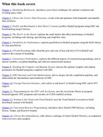
What this book coversChapter 1, Identifying Bottlenecks, introduces you to basic techniques for optimal evaluation andavoiding space leaks.

Chapter 2, Choose the Correct Data Structures, works with and optimizes both immutable and mutabledata structures.

Chapter 3, Profile and Benchmark to Your Heart's Content, profiles Haskell programs using GHC andbenchmarking using Criterion.

Chapter 4, The Devil's in the Detail, explains the small details that affect performance in Haskellprograms, including code sharing, specializing, and simplifier rules.

Chapter 5, Parallelize for Performance, exploits parallelism in Haskell programs using the RePa libraryfor data parallelism.

Chapter 6, I/O and Streaming, talks about the pros and cons of lazy and strict I/O in Haskell andexplores the concept of streaming.

Chapter 7, Concurrency Performance, explores the different aspects of concurrent programming, such asshared variables, exception handling, and software-transactional memory.

Chapter 8, Tweaking the Compiler and Runtime System, chooses the optimal compiler and runtimeparameters for Haskell programs compiled with GHC.

Chapter 9, GHC Internals and Code Optimizations, delves deeper into the compilation pipeline, andunderstands the intermediate representations of GHC.

Chapter 10, Foreign Function Interface, calls safely to and from C in Haskell using GHC and its FFIsupport.

Chapter 11, Programming for the GPU with Accelerate, uses the Accelerate library to programbackend-agnostic GPU programs and executes on CUDA-enabled systems.

Chapter 12, Scaling to the Cloud with Cloud Haskell, uses the Cloud Haskell ecosystem to builddistributed systems with Haskell.

Chapter 13, Functional Reactive Programming, introduces three Haskell FRP libraries, includingElerea, Yampa, and Reactive-banana.

Chapter 14, Library Recommendations, talks about a catalogue of robust Haskell libraries, accompaniedwith overviews and examples.

What you need for this bookTo run most examples in this book, all you need is a working, relatively recent, installation of GHC andsome Haskell libraries. Examples are built for nix-like systems, although they are easily adapted for aWindows machine.

The recommended minimum version for GHC is 7.6. The Haskell libraries needed are introduced in thechapters in which they are used. In Chapter 4, The Devil's in the Detail, we use the Haskell Stack tool toperform some tasks, but it isn't strictly required, although it is recommended to install Stack.

In Chapter 11, Programming for the GPU Using Accelerate, executing the CUDA versions of examplesrequires a CUDA-enabled system and the installation of the CUDA platform.

Who this book is forTo get the most out of this book, you need to have a working knowledge of reading and writing basicHaskell. No knowledge of performance, optimization, or concurrency is required.

ConventionsIn this book, you will find a number of text styles that distinguish between different kinds of information.Here are some examples of these styles and an explanation of their meaning.

Code words in text, database table names, folder names, filenames, file extensions, pathnames, dummyURLs, user input, and Twitter handles are shown as follows: "We can include other contexts through theuse of the include directive."

A block of code is set as follows:

mySum [1..100] = 1 + mySum [2..100] = 1 + (2 + mySum [2..100]) = 1 + (2 + (3 + mySum [2..100])) = ... = 1 + (2 + (... + mySum [100])) = 1 + (2 + (... + (100 + 0)))

When we wish to draw your attention to a particular part of a code block, the relevant lines or items areset in bold:

mySum [1..100] = 1 + mySum [2..100] = 1 + (2 + mySum [2..100]) = 1 + (2 + (3 + mySum [2..100])) = ... = 1 + (2 + (... + mySum [100])) = 1 + (2 + (... + (100 + 0)))

Any command-line input or output is written as follows:

> let xs = enumFromTo 1 5 :: [Int]> :sprint xs

New terms and important words are shown in bold. Words that you see on the screen, for example, inmenus or dialog boxes, appear in the text like this: "Clicking the Next button moves you to the nextscreen."

Note

Warnings or important notes appear in a box like this.

Tip

Tips and tricks appear like this.

Reader feedbackFeedback from our readers is always welcome. Let us know what you think about this book—what youliked or disliked. Reader feedback is important for us as it helps us develop titles that you will really getthe most out of.

To send us general feedback, simply e-mail <feedback@packtpub.com>, and mention the book's title inthe subject of your message.

If there is a topic that you have expertise in and you are interested in either writing or contributing to abook, see our author guide at www.packtpub.com/authors.

Customer supportNow that you are the proud owner of a Packt book, we have a number of things to help you to get the mostfrom your purchase.

Downloading the example codeYou can download the example code files for this book from your account at http://www.packtpub.com.If you purchased this book elsewhere, you can visit http://www.packtpub.com/support and register tohave the files e-mailed directly to you.

You can download the code files by following these steps:

1. Log in or register to our website using your e-mail address and password.2. Hover the mouse pointer on the SUPPORT tab at the top.3. Click on Code Downloads & Errata.4. Enter the name of the book in the Search box.5. Select the book for which you're looking to download the code files.6. Choose from the drop-down menu where you purchased this book from.7. Click on Code Download.

You can also download the code files by clicking on the Code Files button on the book's webpage at thePackt Publishing website. This page can be accessed by entering the book's name in the Search box.Please note that you need to be logged in to your Packt account.

Once the file is downloaded, please make sure that you unzip or extract the folder using the latest versionof:

WinRAR / 7-Zip for WindowsZipeg / iZip / UnRarX for Mac7-Zip / PeaZip for Linux

The code bundle for the book is also hosted on GitHub at https://github.com/PacktPublishing/Haskell-High-Performance-Programming. We also have other code bundles from our rich catalog of books andvideos available at https://github.com/PacktPublishing/. Check them out!

Downloading the color images of this bookWe also provide you with a PDF file that has color images of the screenshots/diagrams used in this book.The color images will help you better understand the changes in the output. You can download this filefromhttp://www.packtpub.com/sites/default/files/downloads/HaskellHighPerformanceProgramming_ColorImages.pdf

ErrataAlthough we have taken every care to ensure the accuracy of our content, mistakes do happen. If you finda mistake in one of our books—maybe a mistake in the text or the code—we would be grateful if youcould report this to us. By doing so, you can save other readers from frustration and help us improvesubsequent versions of this book. If you find any errata, please report them by visitinghttp://www.packtpub.com/submit-errata, selecting your book, clicking on the Errata Submission Formlink, and entering the details of your errata. Once your errata are verified, your submission will beaccepted and the errata will be uploaded to our website or added to any list of existing errata under theErrata section of that title.

To view the previously submitted errata, go to https://www.packtpub.com/books/content/support andenter the name of the book in the search field. The required information will appear under the Erratasection.

PiracyPiracy of copyrighted material on the Internet is an ongoing problem across all media. At Packt, we takethe protection of our copyright and licenses very seriously. If you come across any illegal copies of ourworks in any form on the Internet, please provide us with the location address or website nameimmediately so that we can pursue a remedy.

Please contact us at <copyright@packtpub.com> with a link to the suspected pirated material.

We appreciate your help in protecting our authors and our ability to bring you valuable content.

QuestionsIf you have a problem with any aspect of this book, you can contact us at <questions@packtpub.com>,and we will do our best to address the problem.

Chapter 1. Identifying BottlenecksYou have probably at least once written some very neat Haskell you were very proud of, until you test thecode and it took ages to give an answer or even ran out of memory. This is very normal, especially if youare used to performance semantics in which performance can be analyzed on a step-by-step basis.Analyzing Haskell code requires a different mental model that is more akin to graph traversal.

Luckily, there is no reason to think that writing efficient Haskell is sorcery known only by math wizardsor academics. Most bottlenecks are straightforward to identify with some understanding of Haskell'sevaluation schema. This chapter will help you to reason about the performance of Haskell programs andto avoid some easily recognizable patterns of bad performance:

Understanding lazy evaluation schemas and their implicationsHandling intended and unintended value memoization (CAFs)Utilizing (guarded) recursion and the worker/wrapper pattern efficientlyUsing accumulators correctly to avoid space leaksAnalyzing strictness and space usage of Haskell programsImportant compiler code optimizations, inlining and fusion

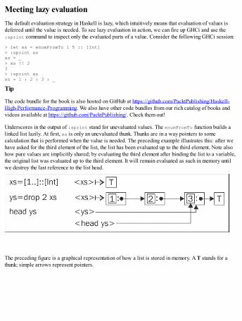
Meeting lazy evaluationThe default evaluation strategy in Haskell is lazy, which intuitively means that evaluation of values isdeferred until the value is needed. To see lazy evaluation in action, we can fire up GHCi and use the:sprint command to inspect only the evaluated parts of a value. Consider the following GHCi session:

> let xs = enumFromTo 1 5 :: [Int]> :sprint xsxs = _> xs !! 23> :sprint xsxs = 1 : 2 : 3 : _

Tip

The code bundle for the book is also hosted on GitHub at https://github.com/PacktPublishing/Haskell-High-Performance-Programming. We also have other code bundles from our rich catalog of books andvideos available at https://github.com/PacktPublishing/. Check them out!

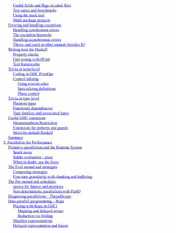
Underscores in the output of :sprint stand for unevaluated values. The enumFromTo function builds alinked list lazily. At first, xs is only an unevaluated thunk. Thunks are in a way pointers to somecalculation that is performed when the value is needed. The preceding example illustrates this: after wehave asked for the third element of the list, the list has been evaluated up to the third element. Note alsohow pure values are implicitly shared; by evaluating the third element after binding the list to a variable,the original list was evaluated up to the third element. It will remain evaluated as such in memory untilwe destroy the last reference to the list head.

The preceding figure is a graphical representation of how a list is stored in memory. A T stands for athunk; simple arrows represent pointers.

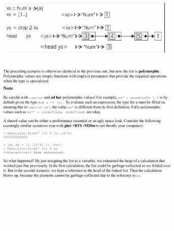
The preceding scenario is otherwise identical to the previous one, but now the list is polymorphic.Polymorphic values are simply functions with implicit parameters that provide the required operationswhen the type is specialized.

Note

Be careful with :sprint and ad hoc polymorphic values! For example, xs' = enumFromTo 1 5 is bydefault given the type Num a => [a]. To evaluate such an expression, the type for a must be filled in,meaning that in :sprint xs', the value xs' is different from its first definition. Fully polymorphicvalues such as xs'' = [undefined, undefined] are okay.

A shared value can be either a performance essential or an ugly space leak. Consider the followingseemingly similar scenarios (run with ghci +RTS -M20m to not throttle your computer):

> Data.List.foldl' (+) 0 [1..10^6]500000500000

> let xs = [1..10^6] :: [Int]> Data.List.foldl' (+) 0 xs<interactive>: Heap exhausted;

So what happened? By just assigning the list to a variable, we exhausted the heap of a calculation thatworked just fine previously. In the first calculation, the list could be garbage-collected as we folded overit. But in the second scenario, we kept a reference to the head of the linked list. Then the calculationblows up, because the elements cannot be garbage-collected due to the reference to xs.

Writing sum correctlyNotice that in the previous example we used a strict variant of left-fold called foldl' from Data.Listand not the foldl exported from Prelude. Why couldn't we have just as well used the latter? After all,we are only asking for a single numerical value and, given lazy evaluation, we shouldn't be doinganything unnecessary. But we can see that this is not the case (again with ghci +RTS -M20m):

> Prelude.foldl (+) 0 [1..10^6]<interactive>: Heap exhausted;

To understand the underlying issue here, let's step away from the fold abstraction for a moment andinstead write our own sum function:

mySum :: [Int] -> IntmySum [] = 0mySum (x:xs) = x + mySum xs

By testing it, we can confirm that mySum too exhausts the heap:

> :load sums.hs> mySum [1..10^6]<interactive>: Heap exhausted;

Because mySum is a pure function, we can expand its evaluation by hand as follows:

mySum [1..100] = 1 + mySum [2..100] = 1 + (2 + mySum [2..100]) = 1 + (2 + (3 + mySum [2..100])) = ... = 1 + (2 + (... + mySum [100])) = 1 + (2 + (... + (100 + 0)))

From the expanded form we can see that we build up a huge sum chain and then start reducing it, startingfrom the very last element on the list. This means that we have all the elements of the list simultaneouslyin memory. From this observation, the obvious thing we could try is to evaluate the intermediate sum ateach step. We could define a mySum2 which does just this:

mySum2 :: Int -> [Int] -> IntmySum2 s [] = smySum2 s (x:xs) = let s' = s + x in mySum2 s' xs

But to our disappointment mySum2 blows up too! Let's see how it expands:

mySum2 0 [1..100] = let s1 = 0 + 1 in mySum2 s1 [2..100] = let s1 = 0 + 1 s2 = s1 + 2 in mySum2 s2 [2..100] ... = let s1 = 0 + 1 ... s100 = s99 + 100 in mySum2 s100 [] = s100

= s99 + 100 = (s89 + 99) + 100 ... = ((1 + 2) + ... ) + 100

Oops! We still build up a huge sum chain. It may not be immediately clear that this is happening. Onecould perhaps expect that 1 + 2 would be evaluated immediately as 3 as it is in strict languages. But inHaskell, this evaluation does not take place, as we can confirm with :sprint:

> let x = 1 + 2 :: Int> :sprint xx = _

Note that our mySum is a special case of foldr and mySum2 corresponds to foldl.

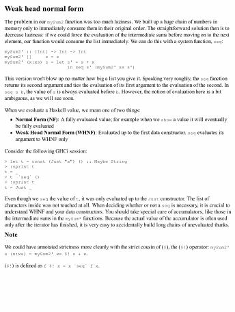
Weak head normal formThe problem in our mySum2 function was too much laziness. We built up a huge chain of numbers inmemory only to immediately consume them in their original order. The straightforward solution then is todecrease laziness: if we could force the evaluation of the intermediate sums before moving on to the nextelement, our function would consume the list immediately. We can do this with a system function, seq:

mySum2' :: [Int] -> Int -> IntmySum2' [] s = smySum2' (x:xs) s = let s' = s + x in seq s' (mySum2' xs s')

This version won't blow up no matter how big a list you give it. Speaking very roughly, the seq functionreturns its second argument and ties the evaluation of its first argument to the evaluation of the second. Inseq a b, the value of a is always evaluated before b. However, the notion of evaluation here is a bitambiguous, as we will see soon.

When we evaluate a Haskell value, we mean one of two things:

Normal Form (NF): A fully evaluated value; for example when we show a value it will eventuallybe fully evaluatedWeak Head Normal Form (WHNF): Evaluated up to the first data constructor. seq evaluates itsargument to WHNF only

Consider the following GHCi session:

> let t = const (Just "a") () :: Maybe String> :sprint tt = _> t `seq` ()> :sprint tt = Just _

Even though we seq the value of t, it was only evaluated up to the Just constructor. The list ofcharacters inside was not touched at all. When deciding whether or not a seq is necessary, it is crucial tounderstand WHNF and your data constructors. You should take special care of accumulators, like those inthe intermediate sums in the mySum* functions. Because the actual value of the accumulator is often usedonly after the iterator has finished, it is very easy to accidentally build long chains of unevaluated thunks.

Note

We could have annotated strictness more cleanly with the strict cousin of ($), the ($!) operator: mySum2's (x:xs) = mySum2' xs $! s + x.

($!) is defined as f $! x = x `seq` f x.

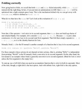
Folding correctlyNow going back to folds, we recall that both foldl and foldr failed miserably, while (+) . foldl'instead did the right thing. In fact, if you just turn on optimizations in GHC then foldl (+) 0 will beoptimized into a tight constant-space loop. This is the mechanism behind why we can get away withPrelude.sum, which is defined as foldl (+) 0.

What do we then have the foldr for? Let's look at the evaluation of foldr f a xs:

foldr f a [x1,x2,x3,x4,...] = f x1 (foldr f a [x2,x3,x4,...]) = f x1 (f x2 (foldr f a [x3,x4,...])) = f x1 (f x2 (f x3 (foldr f a [x4,...]))) …

Note that, if the operator f isn't strict in its second argument, then foldr does not build up chains ofunevaluated thunks. For example, let's consider foldr (:) [] [1..5]. Because (:) is just a dataconstructor, it is for sure lazy in its second (and first) argument. That fold then simply expands to 1 : (2: (3 : ...)), so it is the identity function for lists.

Monadic bind (>>) for the IO monad is another example of a function that is lazy in its second argument:

foldr (>>) (return ()) [putStrLn "Hello", putStrLn "World!"]

For those monads whose actions do not depend on later actions, (that is, printing "Hello" is independentfrom printing "World!" in the IO monad), bind is non-strict in its second argument. On the other hand, thelist monad is an example where bind is generally non-strict in its second argument. (Bind for lists is strictunless the first argument is the empty list.)

To sum up, use a left-fold when you need an accumulator function that is strict in both its operands. Mostof the time, though, a right-fold is the best option. And with infinite lists, right-fold is the only option.

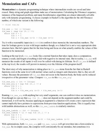
Memoization and CAFsMemoization is a dynamic programming technique where intermediate results are saved and laterreused. Many string and graph algorithms make use of memoization. Calculating the Fibonacci sequence,instances of the knapsack problem, and many bioinformatics algorithms are almost inherently solvableonly with dynamic programming. A classic example in Haskell is the algorithm for the nth Fibonaccinumber, of which one variant is the following:

-- file: fib.hs

fib_mem :: Int -> Integerfib_mem = (map fib [0..] !!) where fib 0 = 1 fib 1 = 1 fib n = fib_mem (n-2) + fib_mem (n-1)

Try it with a reasonable input size (10000) to confirm it does memoize the intermediate numbers. Thetime for lookups grows in size with larger numbers though, so a linked list is not a very appropriate datastructure here. But let's ignore that for the time being and focus on what actually enables the values of thisfunction to be memoized.

Looking at the top level, fib_mem looks like a normal function that takes input, does a computation,returns a result, and forgets everything it did with regard to its internal state. But in reality, fib_mem willmemoize the results of all inputs it will ever be called with during its lifetime. So if fib_mem is definedat the top level, the results will persist in memory over the lifetime of the program itself!

The short story of why memoization is taking place in fib_mem stems from the fact that in Haskellfunctions exist at the same level with normal values such as integers and characters; that is, they are allvalues. Because the parameter of fib_mem does not occur in the function body, the body can be reducedirrespective of the parameter value. Compare fib_mem to this fib_mem_arg:

fib_mem_arg :: Int -> Integerfib_mem_arg x = map fib [0..] !! x where fib 0 = 1 fib 1 = 1 fib n = fib_mem_arg (n-2) + fib_mem_arg (n-1)

Running fib_mem_arg with anything but very small arguments, one can confirm it does no memoization.Even though we can see that map fib [0..] does not depend on the argument number and could bememorized, it will not be, because applying an argument to a function will create a new expression thatcannot implicitly have pointers to expressions from previous function applications. This is equally truewith lambda abstractions as well, so this fib_mem_lambda is similarly stateless:

fib_mem_lambda :: Int -> Integerfib_mem_lambda = \x -> map fib [0..] !! x where fib 0 = 1 fib 1 = 1 fib n = fib_mem_lambda (n-2) + fib_mem_lambda (n-1)

With optimizations, both fib_mem_arg and fib_mem_lambda will get rewritten into a form similar tofib_mem. So in simple cases, the compiler will conveniently fix our mistakes, but sometimes it is

necessary to reorder complex computations so that different parts are memoized correctly.

Tip

Be wary of memoization and compiler optimizations. GHC performs aggressive inlining (Explained inthe section, Inlining and stream fusion) as a routine optimization, so it's very likely that values (andfunctions) get recalculated more often than was intended.

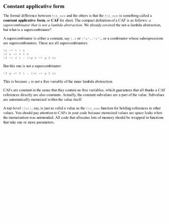
Constant applicative formThe formal difference between fib_mem and the others is that the fib_mem is something called aconstant applicative form, or CAF for short. The compact definition of a CAF is as follows: asupercombinator that is not a lambda abstraction. We already covered the not-a-lambda abstraction,but what is a supercombinator?

A supercombinator is either a constant, say 1.5 or ['a'..'z'], or a combinator whose subexpressionsare supercombinators. These are all supercombinators:

\n -> 1 + n\f n -> f 1 n\f -> f 1 . (\g n -> g 2 n)

But this one is not a supercombinator:

\f g -> f 1 . (\n -> g 2 n)

This is because g is not a free variable of the inner lambda abstraction.

CAFs are constant in the sense that they contain no free variables, which guarantees that all thunks a CAFreferences directly are also constants. Actually, the constant subvalues are a part of the value. Subvaluesare automatically memoized within the value itself.

A top-level [Int], say, is just as valid a value as the fib_mem function for holding references to othervalues. You should pay attention to CAFs in your code because memoized values are space leaks whenthe memoization was unintended. All code that allocates lots of memory should be wrapped in functionsthat take one or more parameters.

Recursion and accumulatorsRecursion is perhaps the most important pattern in functional programming. Recursive functions are morepractical in Haskell than in imperative languages, due to referential transparency and laziness.Referential transparency allows the compiler to optimize the recursion away into a tight inner loop, andlaziness means that we don't have to evaluate the whole recursive expression at once.

Next we will look at a few useful idioms related to recursive definitions: the worker/wrappertransformation, guarded recursion, and keeping accumulator parameters strict.

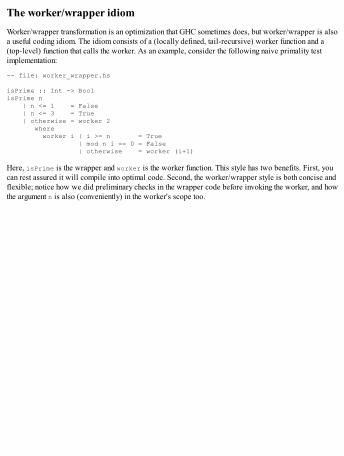
The worker/wrapper idiomWorker/wrapper transformation is an optimization that GHC sometimes does, but worker/wrapper is alsoa useful coding idiom. The idiom consists of a (locally defined, tail-recursive) worker function and a(top-level) function that calls the worker. As an example, consider the following naive primality testimplementation:

-- file: worker_wrapper.hs

isPrime :: Int -> BoolisPrime n | n <= 1 = False | n <= 3 = True | otherwise = worker 2 where worker i | i >= n = True | mod n i == 0 = False | otherwise = worker (i+1)

Here, isPrime is the wrapper and worker is the worker function. This style has two benefits. First, youcan rest assured it will compile into optimal code. Second, the worker/wrapper style is both concise andflexible; notice how we did preliminary checks in the wrapper code before invoking the worker, and howthe argument n is also (conveniently) in the worker's scope too.

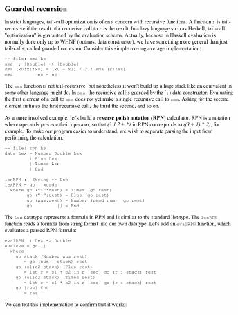
Guarded recursionIn strict languages, tail-call optimization is often a concern with recursive functions. A function f is tail-recursive if the result of a recursive call to f is the result. In a lazy language such as Haskell, tail-call"optimization" is guaranteed by the evaluation schema. Actually, because in Haskell evaluation isnormally done only up to WHNF (outmost data constructor), we have something more general than justtail-calls, called guarded recursion. Consider this simple moving average implementation:

-- file: sma.hssma :: [Double] -> [Double]sma (x0:x1:xs) = (x0 + x1) / 2 : sma (x1:xs)sma xs = xs

The sma function is not tail-recursive, but nonetheless it won't build up a huge stack like an equivalent insome other language might do. In sma, the recursive callis guarded by the (:) data constructor. Evaluatingthe first element of a call to sma does not yet make a single recursive call to sma. Asking for the secondelement initiates the first recursive call, the third the second, and so on.

As a more involved example, let's build a reverse polish notation (RPN) calculator. RPN is a notationwhere operands precede their operator, so that (3 1 2 + *) in RPN corresponds to ((3 + 1) * 2), forexample. To make our program easier to understand, we wish to separate parsing the input fromperforming the calculation:

-- file: rpn.hsdata Lex = Number Double Lex | Plus Lex | Times Lex | End

lexRPN :: String -> LexlexRPN = go . words where go ("*":rest) = Times (go rest) go ("+":rest) = Plus (go rest) go (num:rest) = Number (read num) (go rest) go [] = End

The Lex datatype represents a formula in RPN and is similar to the standard list type. The lexRPNfunction reads a formula from string format into our own datatype. Let's add an evalRPN function, whichevaluates a parsed RPN formula:

evalRPN :: Lex -> DoubleevalRPN = go [] where go stack (Number num rest) = go (num : stack) rest go (o1:o2:stack) (Plus rest) = let r = o1 + o2 in r `seq` go (r : stack) rest go (o1:o2:stack) (Times rest) = let r = o1 * o2 in r `seq` go (r : stack) rest go [res] End = res

We can test this implementation to confirm that it works:

> :load rpn.hs> evalRPN $ lexRPN "5 1 2 + 4 * *"60.0

The RPN expression (5 1 2 + 4 * *) is (5 * ((1 + 2) * 4)) in infix, which is indeed equal to 60.

Note how the lexRPN function makes use of guarded recursion when producing the intermediate structure.It reads the input string incrementally and yields the structure an element at a time. The evaluationfunction evalRPN consumes the intermediate structure from left to right and is tail-recursive, so we keepthe minimum amount of things in memory at all times.

Note

Linked lists equipped with guarded recursion (and lazy I/O) actually provide a lightweight streamingfacility – for more on streaming see Chapter 6, I/O and Streaming.

Accumulator parametersIn our examples so far, we have encountered a few functions that used some kind of accumulator. mySum2had an Int that increased on every step. The go worker function in evalRPN passed on a stack (a linkedlist). The former had a space leak, because we didn't require the accumulator's value until at the end, atwhich point it had grown into a huge chain of pointers. The latter case was okay because the stack didn'tgrow in size indefinitely and the parameter was sufficiently strict in the sense that we didn't unnecessarilydefer its evaluation. The fix we applied in mySum2' was to force the accumulator to WHNF at everyiteration, even though the result was not strictly speaking required in that iteration.

The final lesson is that you should apply special care to your accumulator's strictness properties. If theaccumulator must always be fully evaluated in order to continue to the next step, then you're automaticallysafe. But if there is a danger of an unnecessary chain of thunks being constructed due to a lazyaccumulator, then adding a seq (or a bang pattern, see Chapter 2, Choose the Correct Data Structures)is more than just a good idea.

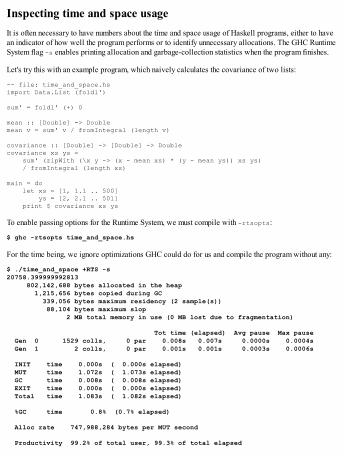
Inspecting time and space usageIt is often necessary to have numbers about the time and space usage of Haskell programs, either to havean indicator of how well the program performs or to identify unnecessary allocations. The GHC RuntimeSystem flag -s enables printing allocation and garbage-collection statistics when the program finishes.

Let's try this with an example program, which naively calculates the covariance of two lists:

-- file: time_and_space.hsimport Data.List (foldl')

sum' = foldl' (+) 0

mean :: [Double] -> Doublemean v = sum' v / fromIntegral (length v)

covariance :: [Double] -> [Double] -> Doublecovariance xs ys = sum' (zipWith (\x y -> (x - mean xs) * (y - mean ys)) xs ys) / fromIntegral (length xs)

main = do let xs = [1, 1.1 .. 500] ys = [2, 2.1 .. 501] print $ covariance xs ys

To enable passing options for the Runtime System, we must compile with -rtsopts:

$ ghc -rtsopts time_and_space.hs

For the time being, we ignore optimizations GHC could do for us and compile the program without any:

$ ./time_and_space +RTS -s20758.399999992813 802,142,688 bytes allocated in the heap 1,215,656 bytes copied during GC 339,056 bytes maximum residency (2 sample(s)) 88,104 bytes maximum slop 2 MB total memory in use (0 MB lost due to fragmentation)

Tot time (elapsed) Avg pause Max pause Gen 0 1529 colls, 0 par 0.008s 0.007s 0.0000s 0.0004s Gen 1 2 colls, 0 par 0.001s 0.001s 0.0003s 0.0006s

INIT time 0.000s ( 0.000s elapsed) MUT time 1.072s ( 1.073s elapsed) GC time 0.008s ( 0.008s elapsed) EXIT time 0.000s ( 0.000s elapsed) Total time 1.083s ( 1.082s elapsed)

%GC time 0.8% (0.7% elapsed)

Alloc rate 747,988,284 bytes per MUT second

Productivity 99.2% of total user, 99.3% of total elapsed

On the first line of output from the Runtime System, we see that we allocated over 800 megabytes ofmemory. This is quite a lot for a program that only handles two lists of 5,000 double-precision values.There is definitely something in our code that could be made a lot more efficient. The output alsocontains other useful information, such as the total memory in use and, more importantly, some statisticson garbage collection. Our program spent only 0.8% of time in GC, meaning the program was doingproductive things 99.2% of the time. So our performance problem lies in the calculations our programperforms themselves.

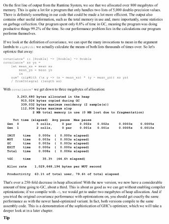
If we look at the definition of covariance, we can spot the many invocations to mean in the argumentlambda to zipWith: we actually calculate the means of both lists thousands of times over. So let'soptimize that away:

covariance' :: [Double] -> [Double] -> Doublecovariance' xs ys = let mean_xs = mean xs mean_ys = mean ys in sum' (zipWith (\x y -> (x - mean_xs) * (y - mean_ys)) xs ys) / fromIntegral (length xs)

With covariance' we get down to three megabytes of allocation:

3,263,680 bytes allocated in the heap 915,024 bytes copied during GC 339,032 bytes maximum residency (2 sample(s)) 112,936 bytes maximum slop 2 MB total memory in use (0 MB lost due to fragmentation)

Tot time (elapsed) Avg pause Max pause Gen 0 5 colls, 0 par 0.002s 0.002s 0.0003s 0.0005s Gen 1 2 colls, 0 par 0.001s 0.001s 0.0005s 0.0010s

INIT time 0.000s ( 0.000s elapsed) MUT time 0.003s ( 0.003s elapsed) GC time 0.003s ( 0.003s elapsed) EXIT time 0.000s ( 0.000s elapsed) Total time 0.008s ( 0.006s elapsed)

%GC time 35.3% (44.6% elapsed)

Alloc rate 1,029,648,194 bytes per MUT second

Productivity 63.1% of total user, 79.6% of total elapsed

That's over a 250-fold decrease in heap allocation! With the new version, we now have a considerableamount of time going to GC, about a third. This is about as good as we can get without enabling compileroptimizations; if we compile with -O, we would get to under two megabytes of heap allocation. And ifyou tried the original covariance performance with optimizations on, you should get exactly the sameperformance as with the newer hand-optimized variant. In fact, both versions compile to the sameassembly code. This is a demonstration of the sophistication of GHC's optimizer, which we will take adeeper look at in a later chapter.

Tip

GHCi tip:

By setting +s in the interpreter, you can get time and space statistics of every evaluation, which can behandy for quick testing. Keep in mind though that no optimizations can be enabled for interpreted code, socompiled code can have very different performance characteristics. To test with optimizations, youshould compile the module with optimizations and then import it into GHCi.

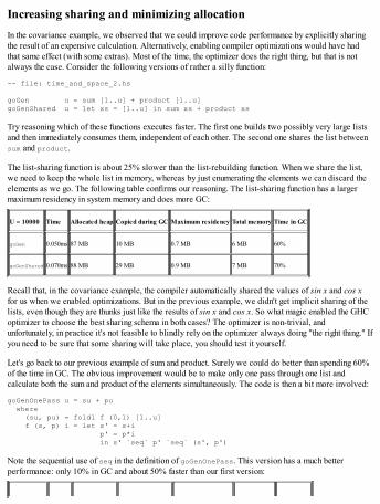
Increasing sharing and minimizing allocationIn the covariance example, we observed that we could improve code performance by explicitly sharingthe result of an expensive calculation. Alternatively, enabling compiler optimizations would have hadthat same effect (with some extras). Most of the time, the optimizer does the right thing, but that is notalways the case. Consider the following versions of rather a silly function:

-- file: time_and_space_2.hs

goGen u = sum [1..u] + product [1..u]goGenShared u = let xs = [1..u] in sum xs + product xs

Try reasoning which of these functions executes faster. The first one builds two possibly very large listsand then immediately consumes them, independent of each other. The second one shares the list betweensum and product.

The list-sharing function is about 25% slower than the list-rebuilding function. When we share the list,we need to keep the whole list in memory, whereas by just enumerating the elements we can discard theelements as we go. The following table confirms our reasoning. The list-sharing function has a largermaximum residency in system memory and does more GC:

U = 10000 Time Allocated heap Copied during GC Maximum residency Total memory Time in GC

goGen 0.050ms 87 MB 10 MB 0.7 MB 6 MB 60%

goGenShared 0.070ms 88 MB 29 MB 0.9 MB 7 MB 70%

Recall that, in the covariance example, the compiler automatically shared the values of sin x and cos xfor us when we enabled optimizations. But in the previous example, we didn't get implicit sharing of thelists, even though they are thunks just like the results of sin x and cos x. So what magic enabled the GHCoptimizer to choose the best sharing schema in both cases? The optimizer is non-trivial, andunfortunately, in practice it's not feasible to blindly rely on the optimizer always doing "the right thing." Ifyou need to be sure that some sharing will take place, you should test it yourself.

Let's go back to our previous example of sum and product. Surely we could do better than spending 60%of the time in GC. The obvious improvement would be to make only one pass through one list andcalculate both the sum and product of the elements simultaneously. The code is then a bit more involved:

goGenOnePass u = su + pu where (su, pu) = foldl f (0,1) [1..u] f (s, p) i = let s' = s+i p' = p*i in s' `seq` p' `seq` (s', p')

Note the sequential use of seq in the definition of goGenOnePass. This version has a much betterperformance: only 10% in GC and about 50% faster than our first version:

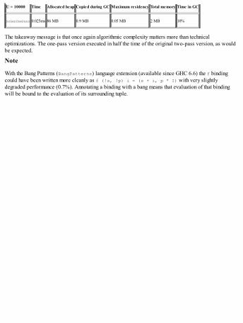
U = 10000 Time Allocated heap Copied during GC Maximum residency Total memory Time in GC

GoGenOnePass 0.025ms 86 MB 0.9 MB 0.05 MB 2 MB 10%

The takeaway message is that once again algorithmic complexity matters more than technicaloptimizations. The one-pass version executed in half the time of the original two-pass version, as wouldbe expected.

Note

With the Bang Patterns (BangPatterns) language extension (available since GHC 6.6) the f bindingcould have been written more cleanly as f (!s, !p) i = (s + i, p * I) with very slightlydegraded performance (0.7%). Annotating a binding with a bang means that evaluation of that bindingwill be bound to the evaluation of its surrounding tuple.

Compiler code optimizationsHaskell compilers perform aggressive optimization transformations on code. GHC optimization passesare highly sophisticated, so much that one rarely needs to worry about performance. We have seen someof the effects of ghc -O1 in our examples so far; in all cases,-O1increased performance relative to nooptimizations, or -Onot, and in some optimizations passes were the difference between constant andexponential complexity.

Inlining and stream fusionGHC performs aggressive inlining, which simply means rewriting a function call with the function'sdefinition. Because all values in Haskell are referentially transparent, any function can be inlined withinthe scope of its definition. Especially in loops, inlining improves performance drastically. The GHCinliner does inlining within a module, but also to some extent cross-module and cross-package.

Some rules of thumb regarding inlining:

If a definition is only used once, and isn't exported, it will always be inlined.When a function body is small, it will almost certainly be inlined no matter where or how often it isused.Bigger functions may be inlined cross-module. To ensure that foo is always inlined, add a {-#INLINE foo #-} pragma near the definition of foo.

With these easy rules, you rarely need to worry about problems from bad inlining. For completeness'ssake, there is also a NOINLINE pragma which ensures a definition is never inlined. NOINLINE is mostlyused for hacks that would break referential transparency; see Chapter 4, The Devil's in the Detail.

Another powerful technique is stream fusion. Behind that fancy name is just a bunch of equations that areused to perform code rewriting (see Chapter 4, The Devil's in the Detail for the technicalities).

When working with lists, you may be tempted to rewrite code like this:

map f . map g . map h

Rather than to use intermediate lists:

map (f . g . h)

But there is no other reason than cosmetics to do this, because with optimizations GHC performs streamfusion, after which both expressions are time- and space-equivalent. Stream fusion is also performed forother structures than [], which we will take a look at in the next chapter.

Polymorphism performanceIn principle, (ad hoc) polymorphic programs should carry a performance cost. To evaluate a polymorphicfunction, a dictionary must be passed in, which contains the specializations for the type specified on thecaller side. However, almost always GHC can fill in the dictionary already at compile time, reducing thecost of polymorphism to zero. The big and obvious exception is code that uses reflection (Typeable).Also, some sufficiently complex polymorphic code might defer the dictionary passing to runtime,although, most of the time you can expect a zero cost.

Either way, it might ease your mind to have some notion of the cost of dictionary passing in runtime. Let'swrite a program with both general and specialized versions of the same function, compile it withoutoptimizations, and compare the performance. Our program will just iterate a simple calculation withdouble-precision values:

-- file: class_performance.hs

class Some a where next :: a -> a -> a

instance Some Double where next a b = (a + b) / 2

goGeneral :: Some a => Int -> a -> agoGeneral 0 x = xgoGeneral n x = goGeneral (n-1) (next x x)

goSpecialized :: Int -> Double -> DoublegoSpecialized 0 x = xgoSpecialized n x = goSpecialized (n-1) (next' x x)

next' :: Double -> Double -> Doublenext' a b = (a + b) / 2

I compiled and ran both versions separately with their own main entry points using the followingcommand lines:

ghc class_performance.hstime ./class_performance +RTS -s

On my machine, with 5,000,000 iterations, the general version does 1.09 GB of allocation and takes 3.4s.The specialized version does 1.01 GB of allocation and runs in about 3.2s. So the extra memory cost wasabout 8%, which is considerable. But by enabling optimizations, both versions will have exactly thesame performance.

Partial functionsHere's a puzzle: given the following definition, which is faster, partial or total?

partialHead :: [a] -> apartialHead (x:_) = x

totalHead :: [a] -> Maybe atotalHead [] = NothingtotalHead (x:_) = Just x

partial = print $ partialHead [1..]

total = print $ case totalHead [1..] of Nothing -> 1 Just n -> n

The total variant uses a head that wraps its result inside a new data constructor, whereas the partialone results in a crash when a case is not matched, but in exchange doesn't perform any extra wrapping.Surely the partial variant must be faster, right? Well, almost always it is not. Both functions have exactlythe same time and space requirements.

Partial functions are justified in some situations, but performance is rarely if ever one of them. In theexample, the Maybe-wrapper of total will have a zero performance cost. The performance cost of thecase analysis will be left, however, but a similar analysis is done in the partial variant too; the error casemust be handled anyway, so that the program can exit gracefully. Of course, even GHC is not a silverbullet and you should always keep in mind that it might miss some optimizations. If you absolutely needto rely on certain optimizations to take place, you should test your program to confirm the correct results.

SummaryIn this chapter, we learned how lazy evaluation works, what weak head normal form is, and how tocontrol it by increasing strictness with different methods. We considered the peculiarities of right-fold,left-fold, and strict left-fold, and in which situations one fold strategy works better than another. Weintroduced the concept of CAF along with memoization techniques, utilized the worker/wrapper pattern,and used guarded recursion to write clean and efficient recursive programs.

We used the :sprint command in GHCi to inspect unevaluated thunks and the Runtime System option -sto inspect the heap usage and GC activity of compiled programs. We took a look at inlining, streamfusion, and the performance costs of partial functions and polymorphism.

In the next chapter, we will take a look at other basic data and control structures, such as different arraystructures and some monads. But first, we will learn about the performance semantics of Haskell datatypes and related common optimization techniques.

Chapter 2. Choosing the Correct Data StructuresPerhaps the next most important topic in Haskell performance after lazy evaluation is data structures. Isay the next most important because although data structures form a wider area than lazy evaluation, theunique performance aspects of lazy evaluation should deserve more attention. Still, structuring dataefficiently is a must for performance, and in Haskell this often requires taking laziness into account, too.

Haskell gives the programmer lots of variety and clutches to structuring data, ranging from low-levelprimitives to ingenious, purely functional data structures. The traditional (re-)implementation costsassociated with quick'n'dirty versus highly optimized solutions are really low in Haskell, and thereforethere are even fewer reasons for complex premature optimizations in Haskell than in many otherlanguages.

This chapter will help you to understand the performance semantics of Haskell values in general and towrite efficient programs for processing numbers, text, and arbitrary data in different classic containerdata types. By the end of this chapter, you will know how to choose and design optimal data structures inapplications. You will be able to drop the level of abstraction in slow parts of code, all the way tomutable data structures if necessary.

This chapter will cover the following points:

Datatype design: boxed and unboxed, strict fields and unpacking fieldsEfficiently processing numeric, binary, and textual dataUsing common sequential, tabular, and mapping container data typesEmploying mutable state in Haskell: IO and ST monadsMonad and monad transformer performance

Annotating strictness and unpacking datatype fieldsRecall that in the previous chapter, we used seq to force strict evaluation. With the BangPatternsextension, we can force functions arguments. Strict arguments are evaluated WHNF just before enteringthe function body:

{-# LANGUAGE BangPatterns #-}

f !s (x:xs) = f (s + 1) xsf !s _ = s

Using bangs for annotating strictness in fact predates the BangPatterns extension (and the oldercompiler flag -fbang-patterns in GHC 6.x). With just plain Haskell98, we are allowed to use bangs tomake datatype fields strict:

> data T = T !Int

A bang in front of a field ensures that whenever the outer constructor (T above) is in WHNF, the innerfield is as well in WHNF. We can check this:

> T undefined `seq` ()*** Exception: Prelude.undefined

There are no restrictions to which fields can be strict, be it recursive or polymorphic fields, although itrarely makes sense to make recursive fields strict. Consider the fully strict linked list:

data List a = List !a !(List a) | ListEnd

With this much strictness, you cannot represent parts of infinite lists without always requiring infinitespace. Moreover, before accessing the head of a finite strict list you must evaluate the list all the way tothe last element. Strict lists don't have the streaming property of lazy lists.

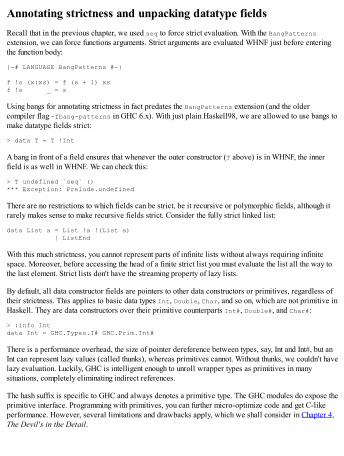
By default, all data constructor fields are pointers to other data constructors or primitives, regardless oftheir strictness. This applies to basic data types Int, Double, Char, and so on, which are not primitive inHaskell. They are data constructors over their primitive counterparts Int#, Double#, and Char#:

> :info Intdata Int = GHC.Types.I# GHC.Prim.Int#

There is a performance overhead, the size of pointer dereference between types, say, Int and Int#, but anInt can represent lazy values (called thunks), whereas primitives cannot. Without thunks, we couldn't havelazy evaluation. Luckily, GHC is intelligent enough to unroll wrapper types as primitives in manysituations, completely eliminating indirect references.

The hash suffix is specific to GHC and always denotes a primitive type. The GHC modules do expose theprimitive interface. Programming with primitives, you can further micro-optimize code and get C-likeperformance. However, several limitations and drawbacks apply, which we shall consider in Chapter 4,The Devil's in the Detail.

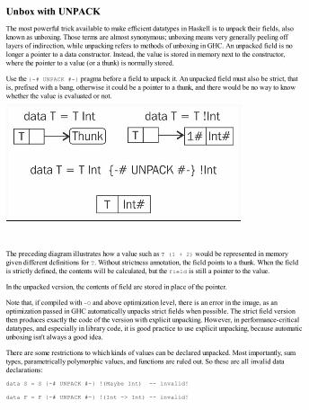
Unbox with UNPACKThe most powerful trick available to make efficient datatypes in Haskell is to unpack their fields, alsoknown as unboxing. Those terms are almost synonymous; unboxing means very generally peeling offlayers of indirection, while unpacking refers to methods of unboxing in GHC. An unpacked field is nolonger a pointer to a data constructor. Instead, the value is stored in memory next to the constructor,where the pointer to a value (or a thunk) is normally stored.

Use the {-# UNPACK #-} pragma before a field to unpack it. An unpacked field must also be strict, thatis, prefixed with a bang, otherwise it could be a pointer to a thunk, and there would be no way to knowwhether the value is evaluated or not.

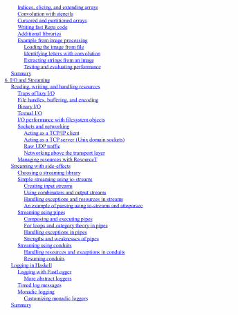
The preceding diagram illustrates how a value such as T (1 + 2) would be represented in memorygiven different definitions for T. Without strictness annotation, the field points to a thunk. When the fieldis strictly defined, the contents will be calculated, but the field is still a pointer to the value.

In the unpacked version, the contents of field are stored in place of the pointer.

Note that, if compiled with -O and above optimization level, there is an error in the image, as anoptimization passed in GHC automatically unpacks strict fields when possible. The strict field versionthen produces exactly the code of the version with explicit unpacking. However, in performance-criticaldatatypes, and especially in library code, it is good practice to use explicit unpacking, because automaticunboxing isn't always a good idea.

There are some restrictions to which kinds of values can be declared unpacked. Most importantly, sumtypes, parametrically polymorphic values, and functions are ruled out. So these are all invalid datadeclarations:

data S = S {-# UNPACK #-} !(Maybe Int) -- invalid!

data F = F {-# UNPACK #-} !(Int -> Int) -- invalid!

data P a = P {-# UNPACK #-} !a -- invalid!

On the other hand, these are valid:

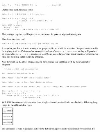
data T = T {-# UNPACK #-} !(Int, Int)

data R a = R { field_a :: a , field_t :: {-# UNPACK #-} !T }data GADT a where Empty :: GADT () Some :: a - > {-# UNPACK #-} !Int - > Some Int

That last type requires enabling the GADTs extension, for general algebraic datatypes.

Then how about this one?

data W = W {-# UNPACK #-} !Int {-# UNPACK #-} !W

It compiles just fine. W is not a sum type nor polymorphic, so it will be unpacked. But you cannot actuallydo anything with W – it's impossible to construct values of type W: W 1 undefined as they will producean error, while let w = W 1 w produces a loop! So as a corollary of other requirements of unboxing, wehave that inductive fields cannot be unpacked.

Now let's find out the effect of unpacking on performance in a tight loop with the following littleprogram:

-- file: strict_and_unpacked.hs

{-# LANGUAGE BangPatterns #-}

data PairP = PairP Int Int deriving (Show)

data PairS = PairS !Int !Int deriving (Show)

data PairU = PairU {-# UNPACK #-} !Int {-# UNPACK #-} !Int deriving (Show)

iter :: Int -> (a -> a) -> a -> aiter end f x = go 0 x where go !n x | n < end = go (n + 1) $! f x | otherwise = x

With 1000 iterations of a function that does simple arithmetic on the fields, we obtain the following heapusage for the different data types:

PairP 370 KB

PairS 50 KB

PairU 50 KB

The difference is very big indeed! But do note that unboxing doesn't always increase performance. For

example, consider a record with a lot of fields. If those fields contain large chunks of unboxed data, thento make a copy of the record would mean duplicating all of that unboxed data too. Comparing to if thosefields were lazy, that is, represented by pointers, we would only need to make copies of those pointers.

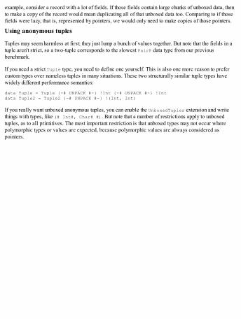
Using anonymous tuples

Tuples may seem harmless at first; they just lump a bunch of values together. But note that the fields in atuple aren't strict, so a two-tuple corresponds to the slowest PairP data type from our previousbenchmark.

If you need a strict Tuple type, you need to define one yourself. This is also one more reason to prefercustom types over nameless tuples in many situations. These two structurally similar tuple types havewidely different performance semantics:

data Tuple = Tuple {-# UNPACK #-} !Int {-# UNPACK #-} !Intdata Tuple2 = Tuple2 {-# UNPACK #-} !(Int, Int)

If you really want unboxed anonymous tuples, you can enable the UnboxedTuples extension and writethings with types, like (# Int#, Char# #). But note that a number of restrictions apply to unboxedtuples, as to all primitives. The most important restriction is that unboxed types may not occur wherepolymorphic types or values are expected, because polymorphic values are always considered aspointers.

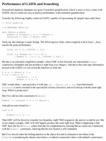
Performance of GADTs and branchingGeneralized algebraic datatypes are great. Existential quantification, which is more or less, comes withGADTs, but it's relatively easy to destroy performance with existential quantification.

Consider the following slightly contrived GADT, capable of representing all integral types and Chars:

-- file: gadts.hs

{-# LANGUAGE GADTs #-}

data Object a where Number :: Integral a => a -> Object a Character :: Char -> Object Char

Turns out, this datatype is quite benign. The following two folds, when compiled with at least-O, haveexactly the same performance:

foldl (+) 0 [1..1000000 :: Int]

foldl (\a (Number b) -> a + b) 0 [ Number x | x <- [1..1000000 :: Int] ]

But this is an extremely simplified example, where GHC in fact discards our intermediate Numberconstructors altogether and just produces a tight loop over integers. And due to the extra type informationpresent in the GADT, we can switch the function we fold into:

f :: a -> Object a -> af a x = case x of Character _ -> a Number n -> a + n

GHC would inline f and specialize it with type Int → Object Int → Int, learn that branchCharacter is never reached in the specialized version, discard it, and we'd end up with the same tightloop. Which is pretty nice!

But if we add an extra constructor to Object:

Number' :: Integral a => a -> Object a

And add an extra branch to f:

case x of … Number' n -> a - n

Then GHC will be forced to consider two branches, right? Well in general, the answer would be yes. Butin our simple example, GHC will still happily produce the same tight loop. What is happening is thatGHC fuses the list of Object values from the list comprehension, learning that no values are constructedwith the Number' constructor, inferring that the new branch is still redundant.

But if we forced either the folding function or the object list and its elements to not inline (withNOINLINE or producing the objects elsewhere), or indeed constructed values with multiple constructors,

then GHC would be forced to consider all type-correct branches.

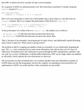
So, in general, GADTs are optimized pretty well. But what about existentials? Consider using thisObjectE instead of Object:

data ObjectE where NumberE :: Integral a => a -> ObjectE

Here we're just saying that we don't care which number type a given object is, only that it has anIntegral instance. But if we compare the performance of this fold over [ObjectE]:

foldl (\a (NumberE b) -> a + fromIntegral b) 0 [ NumberE x | x <- [1..1000000 :: Int] ]

To the performance of a similar fold over [Object Int], the numbers are as follows:

[Object Int]: 51 KB allocated and execution time about 5ms[ObjectE]: 32,000 KB allocated and execution time about 30ms

That is, because of an existential, our program got six times slower, and additionally started allocatingspace linear to input size. What exactly is going on here?

The problem is that by wrapping our numbers inside an existential, we are deliberately forgetting thetype. The type class constraint lets us retain some information, but with an extra cost of a layer ofindirection. Existentials force this indirection to persist through all GHC optimizations, and that's whyour code was so slow. Furthermore, with that added indirection, GHC can no longer unbox our numbersas efficiently, which explains the extra allocations we observed.

The lessons here are that existentials have an overhead, and that extra type information available inGADTs helps not only the programmer, but also the compiler, by opening up extra possibilities foroptimizations. GADT's are useful and fast, while existentials are just useful.

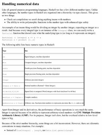
Handling numerical dataLike all general-purpose programming languages, Haskell too has a few different number types. Unlikeother languages, the number types in Haskell are organized into a hierarchy via type classes. This givesus two things:

Check sat compiletime we aren't doing anything insane with numbersThe ability to write polymorphic functions in the number type with enhanced type safety

An example of an insane thing would be dividing an integer by another integer, expecting an integer as aresult. And because every integral type is an instance of the Integral class, we can easily write afactorial function that doesn't care what the underlying type is (as long as it represents an integer):

factorial :: Integral a => a -> afactorial n = product [1..n]

The following table lists basic numeric types in Haskell:

Type Size

Int Signed integers, machine-dependent

Word Unsigned integers, machine-dependent

Double Double-precision floating point, machine-dependent

Float Single-precision floating point, machine-dependent

Integer Arbitrary precision integers

Integral a => Ratio a Rational numbers (Rational = Ratio Integer)

Int/Word{8,16,32,64} Signed (Int) or unsigned (Word) integers with fixed size(from 8 to 64 bits)

RealFloat a => Complex a Complex numbers

HasResolution a => Fixed a Arbitrary size, fixed-precision numbers (a represents precision, like E0, E1, and so on)

Apart from Integer and its derivatives, the performance of basic operations is very much the same.Integer is special because of its ability to represent arbitrary-sized numbers via GNU Multiple PrecisionArithmetic Library (GMP). For its purpose, Integer isn't slow, but the overhead relative to low-leveltypes is big.

Because of the strict number hierarchy, some things are a bit inconvenient. However, there are idiomaticconventions in many situations. For example:

Instead of fromIntegral . length, use Data.List.genericLength

Instead of 1 / fromIntegral (length xs), write 1 % length xsUse float2Double and double2Float from GHC.Float to convert between Floats and Doubles

Loops that use intermediate numbers usually benefit from strictness annotations. GHC often unboxes strictnumber arguments, which leads to efficient code. Strict arguments in non-recursive functions, however,are usually not a good idea, resulting in longer execution times due to suboptimal sharing.

GHC flags that often give better performance for number-heavy code include -O2, -fexcess-precision, and -fllvm. The last flag compiles via LLVM, which requires the LLVM libraries installed(and currently (GHC 7 series) only version 3.5 is supported).

Handling binary and textual dataThe smallest piece of data is a bit (0 or 1), which is isomorphic to Bool (True or False). When youneed just one bit, a Bool should be your choice. If you need a few bits, then a tuple of Bools will fit thepurpose when performance is not critical. A [Bool] is sometimes convenient, but should only be chosenfor convenience in some situations.

For high-performance binary data, you could define your own data type with strict Bool fields. But thishas an important caveat, namely that Bool is not a primitive but an algebraic data type:

data Bool = False | True

The consequence is that you cannot unpack a Bool similar to how you could an Int or Double. In Haskell,Bool values will always be represented by pointers. Fortunately for many bit-fiddling applications, youcan define a data type like this:

data BitStruct = BitStore !Bool !Bool !Bool

This will get respectable performance. However, if you need a whole array of bits it quickly becomesinconvenient to define a field per bit.

Representing bit arraysOne way to define a bit array in Haskell that still retains the convenience of Bool is:

import Data.Array.Unboxedtype BitArray = UArray Int Bool

This representation packs 8 bits per byte, so it's space efficient. See the following section on arrays ingeneral to learn about time efficiency – for now we only note that BitArray is an immutable datastructure, like BitStruct, and that copying small BitStructs is cheaper than copying BitArrays due tooverheads in UArray.

Consider a program that processes a list of integers and tells whether they are even or odd counts ofnumbers divisible by 2, 3, and 5. We can implement this with simple recursion and a three-bitaccumulator. Here are three alternative representations for the accumulator:

-- file: bitstore.hs

{-# LANGUAGE BangPatterns #-}

import Data.Array.Unboxedimport Data.Bits (xor)type BitTuple = (Bool, Bool, Bool)data BitStruct = BitStruct !Bool !Bool !Bool deriving Showtype BitArray = UArray Int Bool

And the program itself is defined along these lines:

go :: acc -> [Int] -> accgo acc [] = accgo (two three five) (x:xs) = go ((test 2 x `xor` two)(test 3 x `xor` three)(test 5 x `xor` five)) xs

test n x = x `mod` n == 0

I've omitted the details here. They can be found in the bitstore.hs file.

The fastest variant is BitStruct, then comes BitTuple (30% slower), and BitArray is the slowest (130%slower than BitStruct). Although BitArray is the slowest (due to making a copy of the array on everyiteration), it would be easy to scale the array in size or make it dynamic. Note also that this benchmark isreally on the extreme side; normally programs do a bunch of other stuff besides updating an array in atight loop.

If you need fast array updates, you can resort to mutable arrays discussed later on. It might also betempting to use Data.Vector.Unboxed.Vector Bool from the vector package, due to its niceinterface. But beware that that representation uses one byte for every bit, wasting 7 bits for every bit.

Handling bytes and blobs of bytesThe next simplest piece of information after bits is a byte, which is eight bits. In Haskell, the Word8 typerepresents a byte. Often though, whole words are more useful. The Word type has the same size as Int,defined by the underlying architecture. Types Word16, Word32, and Word64 consist of respectivenumbers of bits.

Like a bit array, a byte array could be represented as a UArray. But a more standard solution is to useByteString from the bytestring package. The bytestring package uses a blazingly fast pointerrepresentation internally, while the API looks just like the API for standard lists.

Let's test how fast it really is:

-- file: bytestring-perf.hs

import qualified Data.ByteString as Bimport System.IO (stdin)

go :: Int -> Int -> IO Intgo 0 s = return $! sgo n s = do bs <- B.hGet stdin (1024 * 1024) go (n-1) $! B.length bs + s

main = go 2048 0 >>= print

This program reads two gigabytes of binary data from its standard input in one megabyte chunks andprints the total of bytes read. Test it with this:

$ ghc -rtsopts -O bytestring-perf.hs$ time ./bytestring-perf +RTS -s < /dev/zero

On my machine, the program takes 0.25 seconds and allocates about 2.1 gigabytes in heap – meaningthere was hardly any space overhead from our use of ByteString and speed was respectable as well.

The Data.ByteString.ByteString datatype is strict, meaning that all bytes of a ByteString will be inmemory. The Data.ByteString.Lazy module defines its own ByteString, which is lazy:

data ByteString = Empty | Chunk {-# UNPACK #-} !S.ByteString ByteString

Note

Note that you can unbox strict ByteStrings in your own data types as well.

Using lazy ByteStrings, we could rewrite our program as follows:

-- file: bytestring-lazy-perf.hs

import qualified Data.ByteString.Lazy as Bimport qualified Data.ByteString as Simport System.IO (stdin)

size = 2048 * 1024 * 1024

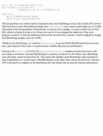
go :: Int -> [S.ByteString] -> Intgo s (c:cs) | s >= size = s | otherwise = go (s + S.length c) cs

main = do bs <- B.hGetContents stdin print $ go 0 (B.toChunks bs)

This program has very similar memory footprint to the strict ByteString version, but is about 20% slower.That slowdown comes from different chunk sizes. hGetContents uses a hard-coded chunk size of 32 KB(described in the documentation of ByteString). In our previous example, we used a chunk size of 1024KB, which is a better fit when a lot of bytes are read in. If you changed the chunk size of the strictprogram variant to 32 KB, the difference between the strict and lazy variants would be negligible, thoughlazy ByteStrings produce more GC traffic.

Thanks to lazy ByteStrings, we could use hGetContents to get an infinite ByteString and turn our loopinto a pure function. Pure code is in general more valuable than just raw performance.

Starting with bytestring 0.10.0.0, the Data.ByteString.Short module provides byte arrays withzero memory overhead. A normal ByteString has a memory overhead of a few Word, and a ByteString,once allocated, cannot be moved by GC. This means that multiple small ByteString could contribute toheap fragmentation, or wasted space. ShortByteString, on the other hand, can be moved by GC, but theirAPI is not nearly as complete as the ByteString API, and should only be used for internal optimization.

Working with characters and stringsThe standard Char data type is defined to hold any character of the ISO 10646 character set. Charrepresents every character with 31 bits.

The text representation chosen in Prelude and base libraries is String = [Char]. This representationhas the convenient property that an understanding of, and operations on, lists carries over to Strings.Furthermore, it's trivial to write programs that process infinite data sequentially without any extralibraries.

Other than being convenient for the programmer, linked lists have a huge overhead, making them ill-suited for high performance string processing. Furthermore, String isn't totally Unicode-correct becausesome strings' lengths depend on their case.

We could fix performance with a UArray ix Char. However, this still wouldn't get us Unicode-correctness.

The bytestring package provides a simple 8-bit character interface for ByteStrings in separate Char8modules (one for strict and lazy ByteStrings), which may sometimes be all you need if you are sure you'reworking with 8-bit (ISO 8859) encoded strings.

Using the text library

The library of choice for general text processing nowadays is text. Its API is designed to resembleString functions, but is faster and Unicode-correct. The Text datatype stores values UTF-16 encoded.That's 16 bits for most characters and 32 bits for obscure characters. Compare this to 31 bits in a Char.

Note

Note that due to the different representations, there is an overhead when converting Strings and Texts. Itdoesn't always make sense to convert from String to Text or vice versa.

Similar to the bytestring library, the text library provides strict and lazy variants under differentmodules. I/O operations with strict and lazy Text are provided under corresponding modules.

Unlike the bytestring library, the text library uses internally an array representation and employs atechnique called stream fusion to eliminate the need for intermediate values. Basically this means thatpipelines such as T.length . T.toUpper . T.init will be optimized into a single loop over the inputvalue when optimizations are enabled. Functions that are fused away are indicated in the documentationof text with the phrase Subject to fusion.

The text-icu package provides bindings for the mature International Components for Unicode (ICU)library on top of text.

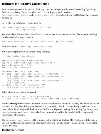
Builders for iterative constructionBuilder abstractions can be used to efficiently compose multiple small chunks into one big ByteString,Text, or even String. The text and bytestring packages provide modules,Data.ByteString.Builder and Data.Text.Lazy.Builder, which define Builder types that composeas monoids.

Say we have a data type, Tree, defined by:

data Tree = Tree !(Int, Tree) !(Int, Tree) | Leaf !ByteString

We want a ByteString serialization of Tree values, so that for an example value (this requires enablingthe OverloadedStrings extension):

Tree (1,Leaf "one") (2, Tree (3,Leaf "three") (4,Leaf "four"))

This encodes as [1:"one",2:[3:"three",4:"four"]].

We can accomplish this with the following function:

-- file: builder-encoding.hs

import Data.ByteString (ByteString)import qualified Data.ByteString.Builder as Bimport Data.Monoid ((<>))import System.IO (stdout)

encodeTree :: Tree -> B.BuilderencodeTree (Tree (l1, t1) (l2, t2)) = B.charUtf8 '[' <> B.intDec l1 <> B.charUtf8 ':'<> encodeTree t1 <> B.charUtf8 ',' <> B.intDec l2 <> B.charUtf8 ':'<> encodeTree t2 <> B.charUtf8 ']'encodeTree (Leaf bs) = B.charUtf8 '"' <> B.byteString bs <> B.charUtf8 '"'

I also added a main to test the encoder:

main = B.hPutBuilder stdout $ encodeTree $ Tree (1,Leaf "one") (2, Tree (3,Leaf "three") (4,Leaf "four"))

The ByteString Builder skips all unnecessary intermediate data structures. A ready Builder value can berendered as a lazy ByteString, meaning it can be consumed lazily. So it's completely possible to createeven infinite ByteStrings with Builder. As a final bonus, if you are writing the resulting ByteString into aHandle, you can use hPutBuilder, which puts the result straight in the handle's buffer, skipping allintermediate allocations.

The Data.Text.Lazy.Builder API is similar to the ByteString Builder API. The biggest difference isthat text Builders can be constructed only from Chars, and lazy and strict Texts, so they're clearly fit fortextual data only.

Builders for strings

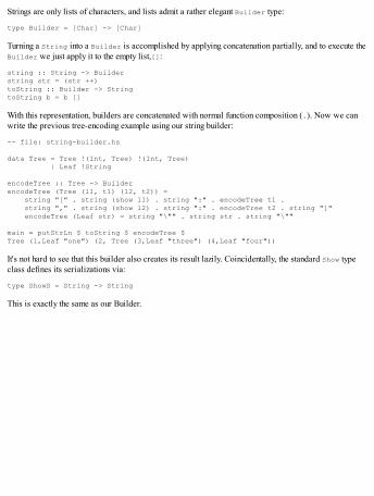
Strings are only lists of characters, and lists admit a rather elegant Builder type:

type Builder = [Char] -> [Char]

Turning a String into a Builder is accomplished by applying concatenation partially, and to execute theBuilder we just apply it to the empty list,[]:

string :: String -> Builderstring str = (str ++)toString :: Builder -> StringtoString b = b []

With this representation, builders are concatenated with normal function composition (.). Now we canwrite the previous tree-encoding example using our string builder:

-- file: string-builder.hs

data Tree = Tree !(Int, Tree) !(Int, Tree) | Leaf !String

encodeTree :: Tree -> BuilderencodeTree (Tree (l1, t1) (l2, t2)) = string "[" . string (show l1) . string ":" . encodeTree t1 . string "," . string (show l2) . string ":" . encodeTree t2 . string "]" encodeTree (Leaf str) = string "\"" . string str . string "\""

main = putStrLn $ toString $ encodeTree $Tree (1,Leaf "one") (2, Tree (3,Leaf "three") (4,Leaf "four"))

It's not hard to see that this builder also creates its result lazily. Coincidentally, the standard Show typeclass defines its serializations via:

type ShowS = String -> String

This is exactly the same as our Builder.

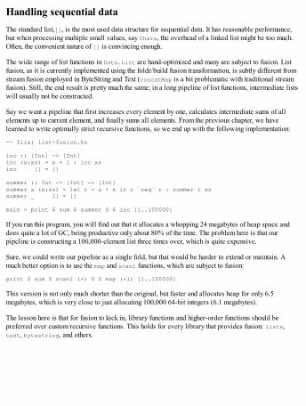
Handling sequential dataThe standard list,[], is the most used data structure for sequential data. It has reasonable performance,but when processing multiple small values, say Chars, the overhead of a linked list might be too much.Often, the convenient nature of [] is convincing enough.

The wide range of list functions in Data.List are hand-optimized and many are subject to fusion. Listfusion, as it is currently implemented using the foldr/build fusion transformation, is subtly different fromstream fusion employed in ByteString and Text (concatMap is a bit problematic with traditional streamfusion). Still, the end result is pretty much the same; in a long pipeline of list functions, intermediate listswill usually not be constructed.

Say we want a pipeline that first increases every element by one, calculates intermediate sums of allelements up to current element, and finally sums all elements. From the previous chapter, we havelearned to write optimally strict recursive functions, so we end up with the following implementation:

-- file: list-fusion.hs

inc :: [Int] -> [Int]inc (x:xs) = x + 1 : inc xsinc [] = []

summer :: Int -> [Int] -> [Int]summer a (x:xs) = let r = a + x in r `seq` r : summer r xssummer _ [] = []

main = print $ sum $ summer 0 $ inc [1..100000]

If you run this program, you will find out that it allocates a whopping 24 megabytes of heap space anddoes quite a lot of GC, being productive only about 80% of the time. The problem here is that ourpipeline is constructing a 100,000-element list three times over, which is quite expensive.

Sure, we could write our pipeline as a single fold, but that would be harder to extend or maintain. Amuch better option is to use the map and scanl functions, which are subject to fusion:

print $ sum $ scanl (+) 0 $ map (+1) [1..100000]

This version is not only much shorter than the original, but faster and allocates heap for only 6.5megabytes, which is very close to just allocating 100,000 64-bit integers (6.1 megabytes).

The lesson here is that for fusion to kick in, library functions and higher-order functions should bepreferred over custom recursive functions. This holds for every library that provides fusion: lists,text, bytestring, and others.

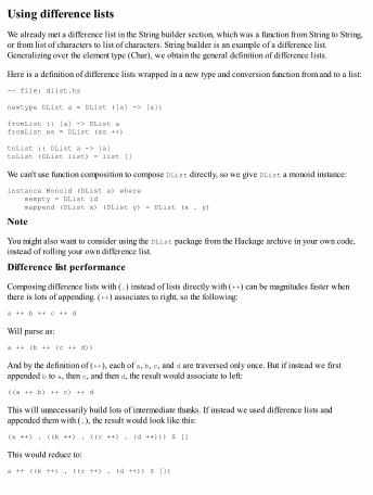
Using difference listsWe already met a difference list in the String builder section, which was a function from String to String,or from list of characters to list of characters. String builder is an example of a difference list.Generalizing over the element type (Char), we obtain the general definition of difference lists.

Here is a definition of difference lists wrapped in a new type and conversion function from and to a list:

-- file: dlist.hs

newtype DList a = DList ([a] -> [a])

fromList :: [a] -> DList afromList xs = DList (xs ++)

toList :: DList a -> [a]toList (DList list) = list []

We can't use function composition to compose DList directly, so we give DList a monoid instance:

instance Monoid (DList a) where mempty = DList id mappend (DList x) (DList y) = DList (x . y)

Note

You might also want to consider using the DList package from the Hackage archive in your own code,instead of rolling your own difference list.

Difference list performance

Composing difference lists with (.) instead of lists directly with (++) can be magnitudes faster whenthere is lots of appending. (++) associates to right, so the following:

a ++ b ++ c ++ d

Will parse as:

a ++ (b ++ (c ++ d))

And by the definition of (++), each of a, b, c, and d are traversed only once. But if instead we firstappended b to a, then c, and then d, the result would associate to left:

((a ++ b) ++ c) ++ d

This will unnecessarily build lots of intermediate thunks. If instead we used difference lists andappended them with (.), the result would look like this:

(a ++) . ((b ++) . ((c ++) . (d ++))) $ []

This would reduce to:

a ++ ((b ++) . ((c ++) . (d ++)) $ [])

And so on, turning (++) right-associative again.

Difference list with the Writer monad

A difference list is often a much better choice as the logging type in a Writer monad. Here is a simplebenchmark of using lists versus difference lists:

-- file: dlist.hs

import Control.Monad.Writer

type DListWriter = Writer (DList Int)type ListWriter = Writer [Int]

action :: Int -> ListWriter ()action 15000 = return ()action n = action (n + 1) >> tell [n]

action' :: Int -> DListWriter ()action' 15000 = return ()action' n = action' (n + 1) >> tell (fromList [n])main = do forM (snd $ runWriter (action 1)) print -- [] forM (toList $ snd $ runWriter (action' 1)) print -- DList

The list-based version starts printing the numbers at an almost readable speed and gradually gains speed,while the difference list-based version spits out numbers immediately.

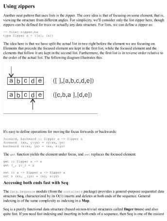
Using zippersAnother neat pattern that uses lists is the zipper. The core idea is that of focusing on some element, that is,viewing the structure from different angles. For simplicity, we'll consider only the list zipper here, thoughzippers can be defined for trees or actually any data structure. For lists, we can define a zipper as:

-- file: zipper.hs type Zipper a = ([a], [a])

The idea here is that we have split the actual list in two right before the element we are focusing on.Elements that precede the focused element are kept in the first list, while the focused element and theelements that follow it are kept in the second list. Furthermore, the first list is in reverse order relative tothe order of the actual list. The following diagram illustrates this:

It's easy to define operations for moving the focus forwards or backwards:

forward, backward :: Zipper a -> Zipper aforward (xs, y:ys) = (y:xs, ys)backward (x:xs, ys) = (xs, x:ys)

The get function yields the element under focus, and set replaces the focused element:

get :: Zipper a -> aget (_, y:_) = y

set :: a -> Zipper a -> Zipper aset x (xs, _:ys) = (xs, x:ys)

Accessing both ends fast with Seq

The Data.Sequence module (from the containers package) provides a general-purpose sequential datastructure Seq, characterized by its O(1) inserts and deletes at both ends of the sequence. Generalindexing is of the same complexity as indexing in a Map.

Seq is a purely functional data structure (based on non-trivial structures called finger trees) and alsoquite fast. If you need fast indexing and inserting in both ends of a sequence, then Seq is one of the easiest

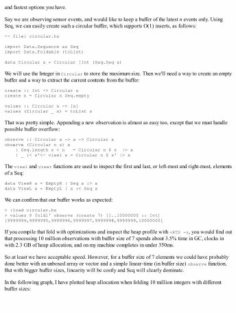
and fastest options you have.

Say we are observing sensor events, and would like to keep a buffer of the latest n events only. UsingSeq, we can easily create such a circular buffer, which supports O(1) inserts, as follows:

-- file: circular.hs

import Data.Sequence as Seqimport Data.Foldable (toList)

data Circular a = Circular !Int (Seq.Seq a)

We will use the Integer in Circular to store the maximum size. Then we'll need a way to create an emptybuffer and a way to extract the current contents from the buffer:

create :: Int -> Circular acreate n = Circular n Seq.empty

values :: Circular a -> [a]values (Circular _ s) = toList s

That was pretty simple. Appending a new observation is almost as easy too, except that we must handlepossible buffer overflow:

observe :: Circular a -> a -> Circular aobserve (Circular n s) x | Seq.length s < n = Circular n $ s |> x | _ :< s'<- viewl s = Circular n $ s' |> x

The viewl and viewr functions are used to inspect the first and last, or left-most and right-most, elementsof a Seq:

data ViewR a = EmptyR | Seq a :> adata ViewL a = EmptyL | a :< Seq a

We can confirm that our buffer works as expected:

> :load circular.hs> values $ foldl' observe (create 7) [1..10000000 :: Int][9999994,9999995,9999996,9999997,9999998,9999999,10000000]

If you compile that fold with optimizations and inspect the heap profile with +RTS -s, you would find outthat processing 10 million observations with buffer size of 7 spends about 3.5% time in GC, clocks inwith 2.3 GB of heap allocation, and on my machine completes in under 350ms.

So at least we have acceptable speed. However, for a buffer size of 7 elements we could have probablydone better with an unboxed array or vector and a simple linear-time (in buffer size) observe function.But with bigger buffer sizes, linearity will be costly and Seq will clearly dominate.

In the following graph, I have plotted heap allocation when folding 10 million integers with differentbuffer sizes:

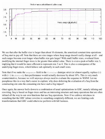
We see that after the buffer size is larger than about 10 elements, the amortized constant time operationsof Seq start to pay off. Note that there are size ranges where heap usage doesn't really change at all – andsuch ranges become even longer when buffer size gets larger! With small buffer sizes, overhead frommodifying the internal finger-trees is far greater than added value. There is even a peak at buffer size 3,implying that it would be more efficient to represent size 3 as 4. This is also a consequence of theunderlying finger-trees, which behave sub optimally in such small sizes.

Note that if we make the sequence field in the Circular datatype strict (or almost equally, replace ($)with ($!) in observe), then performance would actually decrease by about 10%. This is very muchcounterintuitive, because we will anyways always need to evaluate the sequence to WHNF. Let meparaphrase this in a way that's easier to explain: why does deferring the evaluation of a Seq from theconstructing site onto the consuming site have such a big impact?

Once again, the answer boils down to a combination of usual optimizations in GHC, namely inlining andrewriting. Seq is based on finger-trees and has an interesting structure and many operations that are ofteninlined all the way to our own functions that use Seq operations. Now if we enforce strictness insomething that the GHC inliner rewrites to something completely different, we are limiting codetransformations that GHC could otherwise perform with full laziness.

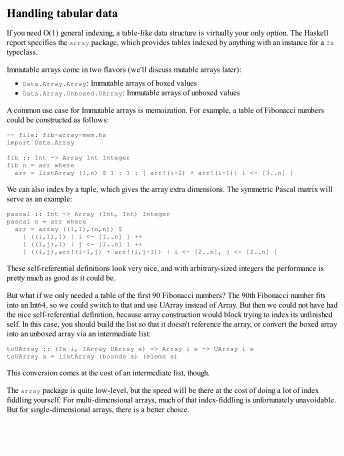
Handling tabular dataIf you need O(1) general indexing, a table-like data structure is virtually your only option. The Haskellreport specifies the array package, which provides tables indexed by anything with an instance for a Ixtypeclass.

Immutable arrays come in two flavors (we'll discuss mutable arrays later):

Data.Array.Array: Immutable arrays of boxed valuesData.Array.Unboxed.UArray: Immutable arrays of unboxed values

A common use case for Immutable arrays is memoization. For example, a table of Fibonacci numberscould be constructed as follows:

-- file: fib-array-mem.hsimport Data.Array

fib :: Int -> Array Int Integerfib n = arr where arr = listArray (1,n) $ 1 : 1 : [ arr!(i-2) + arr!(i-1)| i <- [3..n] ]

We can also index by a tuple, which gives the array extra dimensions. The symmetric Pascal matrix willserve as an example:

pascal :: Int -> Array (Int, Int) Integerpascal n = arr where arr = array ((1,1),(n,n)) $ [ ((i,1),1) | i <- [1..n] ] ++ [ ((1,j),1) | j <- [1..n] ] ++ [ ((i,j),arr!(i-1,j) + arr!(i,j-1)) | i <- [2..n], j <- [2..n] ]

These self-referential definitions look very nice, and with arbitrary-sized integers the performance ispretty much as good as it could be.

But what if we only needed a table of the first 90 Fibonacci numbers? The 90th Fibonacci number fitsinto an Int64, so we could switch to that and use UArray instead of Array. But then we could not have hadthe nice self-referential definition, because array construction would block trying to index its unfinishedself. In this case, you should build the list so that it doesn't reference the array, or convert the boxed arrayinto an unboxed array via an intermediate list:

toUArray :: (Ix i, IArray UArray e) => Array i e -> UArray i etoUArray a = listArray (bounds a) (elems a)

This conversion comes at the cost of an intermediate list, though.

The array package is quite low-level, but the speed will be there at the cost of doing a lot of indexfiddling yourself. For multi-dimensional arrays, much of that index-fiddling is unfortunately unavoidable.But for single-dimensional arrays, there is a better choice.

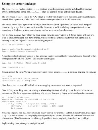
Using the vector packageThe Data.Vector modules in the vector package provide sweet and speedy high-level Int-indexedarrays, implemented on top of Data.Array. They too come in boxed and unboxed flavors.

The sweetness of vector is in the API, which is loaded with higher-order functions, convenient helpers,monad-lifted operations, and of course all the common operations for list-like structures.

The speed comes once again from fusion; in terms of raw speed, operations on vector have an upperbound set by arrays that vectors use internally. However, a sufficiently large composition of vectoroperations will almost always outperform a similar naive array-based program.

Say we have a sensor from which we have stored numeric observations at different times, and now wewant to analyze that data. For performance, we choose to use unboxed vector for storing the data inmemory. Also, we import randomIO for testing purposes:

-- file: vector-testing.hs

import qualified Data.Vector.Unboxed as Uimport System.Random (randomIO)

A neat thing about unboxed Vectors is that unboxed vectors support tuple-valued elements. Internally, theyare represented with two vectors. This defines some types:

type Obs = U.Vector (TimeStamp, Double)

type TimeStamp = Int

We can extract the value Vector of our observation vector using U.unzip in constant time and no copying:

-- | O(1)values :: Obs -> U.Vector Doublevalues obs = snd (U.unzip obs)

Note that U.map snd would be bad, because mapping constructs a new vector, in general.

Now let's try something more interesting: a windowing function, which gives us the slice between twotimestamps. The following implementation of a window function is linear in time and constant in space:

-- | O(n+m), no copying.window :: TimeStamp -> TimeStamp -> Obs -> Obswindow from until v = let (_, start) = U.span ((< from) . fst) v (between, _) = U.span ((<= until) . fst) start in between

We could improve this by a more involved binary search, for example. But for demonstration, I used justU.span, which also does no copying by reusing the original vector. Because the time step between twoobservations (TimeStamps) can be arbitrary, logarithmic time complexity is the best we could get.

Implementing value average is straightforward:

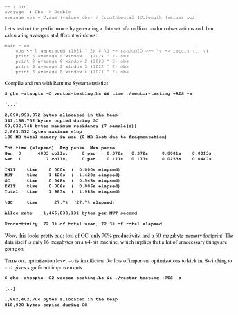
-- | O(n)average :: Obs -> Doubleaverage obs = U.sum (values obs) / fromIntegral (U.length (values obs))

Let's test out the performance by generating a data set of a million random observations and thencalculating averages at different windows:

main = do obs <- U.generateM (1024 ^ 2) $ \i -> randomIO >>= \v -> return (i, v) print $ average $ window 1 (1024 ^ 2) obs print $ average $ window 2 (1023 ^ 2) obs print $ average $ window 3 (1022 ^ 2) obs print $ average $ window 4 (1021 ^ 2) obs

Compile and run with Runtime System statistics:

$ ghc -rtsopts -O vector-testing.hs && time ./vector-testing +RTS -s

[...]

2,090,993,872 bytes allocated in the heap341,188,752 bytes copied during GC59,032,744 bytes maximum residency (7 sample(s))2,863,512 bytes maximum slop138 MB total memory in use (0 MB lost due to fragmentation)

Tot time (elapsed) Avg pause Max pauseGen 0 4003 colls, 0 par 0.372s 0.372s 0.0001s 0.0013sGen 1 7 colls, 0 par 0.177s 0.177s 0.0253s 0.0447s

INIT time 0.000s ( 0.000s elapsed)MUT time 1.426s ( 1.428s elapsed)GC time 0.548s ( 0.548s elapsed)EXIT time 0.006s ( 0.006s elapsed)Total time 1.983s ( 1.983s elapsed)

%GC time 27.7% (27.7% elapsed)

Alloc rate 1,465,833,131 bytes per MUT second

Productivity 72.3% of total user, 72.3% of total elapsed

Wow, this looks pretty bad: lots of GC, only 70% productivity, and a 60-megabyte memory footprint! Thedata itself is only 16 megabytes on a 64-bit machine, which implies that a lot of unnecessary things aregoing on.

Turns out, optimization level -O is insufficient for lots of important optimizations to kick in. Switching to-O2 gives significant improvements:

$ ghc -rtsopts -O2 vector-testing.hs && ./vector-testing +RTS -s

[..]

1,862,402,704 bytes allocated in the heap818,920 bytes copied during GC

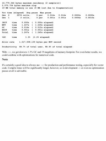
16,779,344 bytes maximum residency (2 sample(s))2,070,704 bytes maximum slop19 MB total memory in use (0 MB lost due to fragmentation)

Tot time (elapsed) Avg pause Max pauseGen 0 3576 colls, 0 par 0.014s 0.014s 0.0000s 0.0000sGen 1 2 colls, 0 par 0.001s 0.001s 0.0006s 0.0010s

INIT time 0.000s ( 0.000s elapsed)MUT time 1.227s ( 1.229s elapsed)GC time 0.016s ( 0.015s elapsed)EXIT time 0.001s ( 0.001s elapsed)Total time 1.247s ( 1.245s elapsed)

%GC time 1.3% (1.2% elapsed)

Alloc rate 1,517,508,130 bytes per MUT second

Productivity 98.7% of total user, 98.9% of total elapsed

With -O2, we got down to 1.3% GC and 19 megabytes of memory footprint. For even better results, wecould combine with optimizations for numerical code.

Note

It's certainly a good idea to always use -O2 for production and performance testing, especially for vectorcode. Compile times will be significantly longer, however, so in development -O or even no optimizationpasses at all is advisable.

Handling sparse dataVectors and arrays are excellent for dense data, that is, when you're not doing inserts in betweenelements, and the range of indices is reasonable. But if you need, for example, inserts and indexing inarbitrary indices, a tabular structure won't perform well. In such cases, you need some sort of a map orsimilar structure.

Haskell doesn't have any sparse structures built-in, nor does the Haskell report define any. This has somenice consequences:

Keeps the core language smallGives Haskellers complete freedom over the implementationAllows writing code that doesn't care much about the specific underlying data structure

There are many excellent libraries, implementing a wide range of sparse data structures, in Hackage, notto mention type classes capturing general properties of those structures. Unfortunately, the ecosystem is abit too scattered, so it is sometimes hard to determine which library would give the best performance,cleanest code, and most flexibility, or whether the package is maintained.

Using the containers packageThe go-to package for immutable sparse data structures is containers. It provides reasonably efficientimplementations for maps and sets, very basic tree and graph structures, and the sequence mentionedpreviously. The structures are purely functional, which is a nice property in itself, encouraging us towrite code in a functional style:

Ord a => Data.Map.{Lazy,Strict}.Map k vOrd a => Data.Set.Set a

Data.IntMap.{Lazy,Strict}.IntMap vData.IntSet.IntSet a

Data.Tree.Tree aData.Graph.Graph = Array Int [Int]Data.Sequence.Seq a

However, you shouldn't expect these structures, say Map, to perform equally with traditional imperative-style structures (hashmaps), especially when used more or less imperatively. The Map from containersis based on binary trees. IntMap, which constrains its keys to Ints, uses Patricia trees and is considerablymore efficient than Map Int.

The imperative map implementation is usually a hash table because of its O(1) lookups compared to theO(log n) of tree-based maps. However, hash tables rely on mutable state, and so are not so convenient infunctional settings.

Functional structures have their unique advantages:

Updates reuse parts of the previous structure, so keeping older versions lying around is cheapAutomatic thread-safety

Furthermore, with lazy evaluation, a map lazy in its values allows for an intuitive memoization pattern:

-- file: map-fib.hs

import Data.IntMap as IM

fib :: Int -> IntMap Intfib n = m where m = IM.fromList $ (1,1) : (2,1) : [ (i, IM.findWithDefault 0 (i-1) m + IM.findWithDefault 0 (i-2) m) | i <- [3..n] ]

Note

Unless you need to have thunks as values, you should use the strict variants of Map and IntMap forefficiency.

Using the unordered-containers packageThe containers package requires an Ord instance from the keys in a Map and from values in a Set. Forstring-valued data this is problematic, because a comparison might be too expensive. And for some data,an Ord instance is an impossibility:

Hashable k => Data.HashMap.Lazy.HashMap k vHashable k => Data.HashMap.Strict.HashMap k vHashable a => Data.HashSet.HashSet

The unordered-containers package provides pure functional hash maps and sets, requiring aHashable instance. The same performance considerations apply to HashMap and HashSet as the datastructures from containers: they are persistent in nature but won't beat mutable-state variants in termsof raw speed.

Ephemeral data structuresLazy evaluation, functional code, and persistent data structures are nice and all, but they are not meant towholly replace imperative strict evaluation, imperative code, and ephemeral structures. Nor vice versa.Instead, all complement each other. Although the default evaluation in Haskell is strict and a functionalstyle is strongly encouraged, Haskell is more than capable of providing for programming in imperativestyle:

"In short, Haskell is the world's finest imperative programming language."

--Simon Peyton Jones (in his paper Tackling the Awkward Squad)

Imperative programming calls for sequential processing. In Haskell, we tackle sequential steps withmonads. The monad of choice for ephemeral data structures is IO or ST. ST (for state threads) behavesa bit more nicely than IO in that you cannot launch missiles from ST. An ST action can be executed inpure code, or converted to an IO action:

import Control.Monad.ST

runST :: (forall s. ST s a) -> astToIO :: ST RealWorld a -> IO a

The s type variable in ST actions can be largely ignored. It is only used to separate the states of separateST actions.

The ST monad comes in two flavors, strict (Control.Monad.ST) and lazy (Control.Monad.ST.Lazy).The lazy ST monad executes only actions whose values are required. The following code works with alazy ST monad, but not with a strict one:

st :: Intst = runST $ do mapM_ return [1..] return 9001

Unless you need lazy semantics, strict ST will be faster.

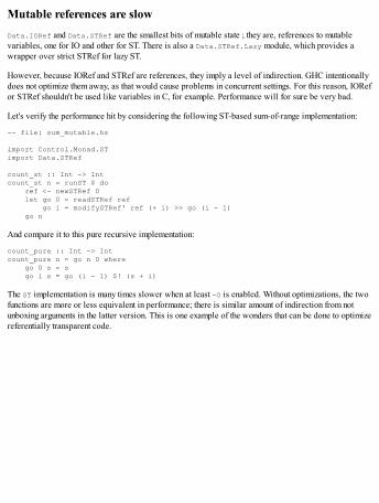
Mutable references are slowData.IORef and Data.STRef are the smallest bits of mutable state ; they are, references to mutablevariables, one for IO and other for ST. There is also a Data.STRef.Lazy module, which provides awrapper over strict STRef for lazy ST.

However, because IORef and STRef are references, they imply a level of indirection. GHC intentionallydoes not optimize them away, as that would cause problems in concurrent settings. For this reason, IORefor STRef shouldn't be used like variables in C, for example. Performance will for sure be very bad.

Let's verify the performance hit by considering the following ST-based sum-of-range implementation:

-- file: sum_mutable.hs

import Control.Monad.STimport Data.STRef

count_st :: Int -> Intcount_st n = runST $ do ref <- newSTRef 0 let go 0 = readSTRef ref go i = modifySTRef' ref (+ i) >> go (i - 1) go n

And compare it to this pure recursive implementation:

count_pure :: Int -> Intcount_pure n = go n 0 where go 0 s = s go i s = go (i - 1) $! (s + i)

The ST implementation is many times slower when at least -O is enabled. Without optimizations, the twofunctions are more or less equivalent in performance; there is similar amount of indirection from notunboxing arguments in the latter version. This is one example of the wonders that can be done to optimizereferentially transparent code.

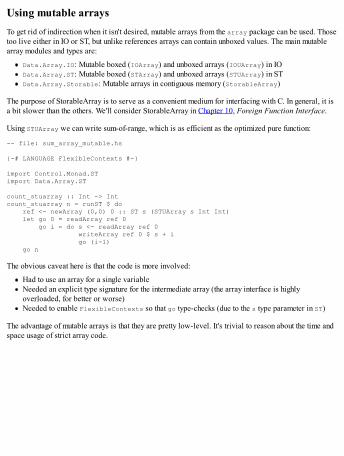
Using mutable arraysTo get rid of indirection when it isn't desired, mutable arrays from the array package can be used. Thosetoo live either in IO or ST, but unlike references arrays can contain unboxed values. The main mutablearray modules and types are:

Data.Array.IO: Mutable boxed (IOArray) and unboxed arrays (IOUArray) in IOData.Array.ST: Mutable boxed (STArray) and unboxed arrays (STUArray) in STData.Array.Storable: Mutable arrays in contiguous memory (StorableArray)

The purpose of StorableArray is to serve as a convenient medium for interfacing with C. In general, it isa bit slower than the others. We'll consider StorableArray in Chapter 10, Foreign Function Interface.

Using STUArray we can write sum-of-range, which is as efficient as the optimized pure function:

-- file: sum_array_mutable.hs

{-# LANGUAGE FlexibleContexts #-}

import Control.Monad.STimport Data.Array.ST

count_stuarray :: Int -> Intcount_stuarray n = runST $ do ref <- newArray (0,0) 0 :: ST s (STUArray s Int Int) let go 0 = readArray ref 0 go i = do s <- readArray ref 0 writeArray ref 0 $ s + i go (i-1) go n

The obvious caveat here is that the code is more involved:

Had to use an array for a single variableNeeded an explicit type signature for the intermediate array (the array interface is highlyoverloaded, for better or worse)Needed to enable FlexibleContexts so that go type-checks (due to the s type parameter in ST)

The advantage of mutable arrays is that they are pretty low-level. It's trivial to reason about the time andspace usage of strict array code.

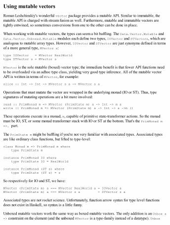
Using mutable vectorsRoman Leshchinskiy's wonderful vector package provides a mutable API. Similar to immutable, themutable API is charged with stream fusion as well. Furthermore, mutable and immutable vectors aretightly entwined, so sometimes conversions from one to the other can be done in place.

When working with mutable vectors, the types can seem a bit baffling. The Data.Vector.Mutable andData.Vector.Unboxed.Mutable modules each define two types, IOVector and STVectors, which areanalogous to mutable array types. However, IOVector and STVector are just synonyms defined in termsof a more general type, MVector s:

type IOVector = MVector RealWorldtype STVector s = MVector s

MVector is the sole mutable (boxed) vector type; the immediate benefit is that fewer API functions needto be overloaded via an adhoc type class, yielding very good type inference. All of the mutable vectorAPI is written in terms of MVector, for example:

slice :: Int -> Int -> MVector s a -> MVector s a

Operations that must mutate the vector are wrapped in the underlying monad (IO or ST). Thus, typesignatures of mutating operations are a bit more involved:

read :: PrimMonad m => MVector (PrimState m) a -> Int -> m awrite :: PrimMonad m => MVector (PrimState m) a -> Int -> a ->m ()

These operations execute in a monad, m, capable of primitive state-transformer actions. So the monadmust be IO, ST, or some monad transformer stack with IO or ST at the bottom. That's the PrimMonad m=>… part.

The PrimState m might be baffling if you're not very familiar with associated types. Associated typesare like ordinary class functions, but lifted to type-level:

class Monad m => PrimMonad m where type PrimState m

instance PrimMonad IO where type PrimState IO = RealWorld

instance PrimMonad (ST s) where type PrimState (ST s) = s

So respectively for IO and ST, we have:

MVector (PrimState m) a === MVector RealWorld a = IOVector aMVector (PrimState m) a === MVector s a = STVector s a

Associated types are not rocket science. Unfortunately, function arrow syntax for type level functionsdoes not exist in Haskell, so syntax is a little funny.

Unboxed mutable vectors work the same way as boxed mutable vectors. The only addition is an Unbox a=> constraint on the element (and the unboxed MVector is a type-family instead of a datatype). Unbox

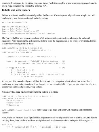
comes with instances for primitive types and tuples (and it is possible to add your own instances), and isalso a requirement in the immutable unboxed API.

Bubble sort with vectors

Bubble sort is not an efficient sort algorithm, but because it's an in-place algorithm and simple, we willimplement it as a demonstration of mutable vectors:

-- file: bubblesort.hs

import Control.Monad.STimport Data.Vector as Vimport Data.Vector.Mutable as MVimport System.Random (randomIO) -- for testing

The (naive) bubble sort compares values of all adjacent indices in order, and swaps the values ifnecessary. After reaching the last element, it starts from the beginning or, if no swaps were made, the listis sorted and the algorithm is done:

bubblesortM :: (Ord a, PrimMonad m) => MVector (PrimState m) a -> m ()bubblesortM v = loop where

indices = V.fromList [1 .. MV.length v - 1]

loop = do swapped <- V.foldM' f False indices – (1) if swapped then loop else return () – (2)

f swapped i = do – (3) a <- MV.read v (i-1) b <- MV.read v i if a > b then MV.swap v (i-1) i >> return True else return swapped

At (1), we fold monadically over all but the last index, keeping state about whether or not we haveperformed a swap in this iteration. If we had, at (2) we rerun the fold ; if not, we can return. At (3) wecompare an index and possibly swap values.

We can write a pure function that wraps the stateful algorithm:

bubblesort :: Ord a => Vector a -> Vector abubblesort v = runST $ do mv <- V.thaw v bubblesortM mv V.freeze mv

V.thaw and V.freeze (both O(n)) can be used to go back and forth with mutable and immutablevectors.

Now, there are multiple code optimization opportunities in our implementation of bubble sort. But beforetackling those, let's see how well our straightforward implementation fares using the following main:

main = do v <- V.generateM 10000 $ \_ -> randomIO :: IO Double

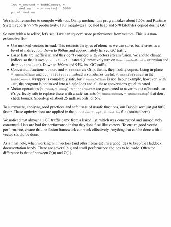
let v_sorted = bubblesort v median = v_sorted ! 5000 print median

We should remember to compile with -O2. On my machine, this program takes about 1.55s, and RuntimeSystem reports 99.9% productivity, 18.7 megabytes allocated heap and 570 kilobytes copied during GC.

So now with a baseline, let's see if we can squeeze more performance from vectors. This is a non-exhaustive list:

Use unboxed vectors instead. This restricts the types of elements we can store, but it saves us alevel of indirection. Down to 960ms and approximately halved GC traffic.Large lists are inefficient, and they don't compose with vectors stream fusion. We should changeindices so that it uses V.enumFromTo instead (alternatively turn on OverloadedLists extension anddrop V.fromList). Down to 360ms and 94% less GC traffic.Conversion functions V.thaw and V.freeze are O(n), that is, they modify copies. Using in-placeV.unsafeThaw and V.unsafeFreeze instead is sometimes useful. V.unsafeFreeze in thebubblesort wrapper is completely safe, but V.unsafeThaw is not. In our example, however, with-O2, the program is optimized into a single loop and all those conversions get eliminated.Vector operations (V.read, V.swap) in bubblesortM are guaranteed to never be out of bounds, soit's perfectly safe to replace these with unsafe variants (V.unsafeRead, V.unsafeSwap) that don'tcheck bounds. Speed-up of about 25 milliseconds, or 5%.

To summarize, applying good practices and safe usage of unsafe functions, our Bubble sort just got 80%faster. These optimizations are applied in the bubblesort-optimized.hs file (omitted here).

We noticed that almost all GC traffic came from a linked list, which was constructed and immediatelyconsumed. Lists are bad for performance in that they don't fuse like vectors. To ensure good vectorperformance, ensure that the fusion framework can work effectively. Anything that can be done with avector should be done.

As a final note, when working with vectors (and other libraries) it's a good idea to keep the Haddockdocumentation handy. There are several big and small performance choices to be made. Often thedifference is that of between O(n) and O(1).

Working with monads and monad stacksMonads are very useful abstractions, and like any sufficiently complex abstraction, many monads tooincur some overhead. Two notable exceptions are IO and ST, which are eliminated during compilation. Asingle simple monad such as Reader or Writer has very minimal overhead, but monad stacks can incurunfortunate slowdowns. In most cases, the convenient nature of programming in a monad stack faroutweighs the small overhead, because cost centers are rarely located in monad operations (excluding IOand ST).

Note

If you have an expensive subroutine in a State monad, it might be possible to convert it to ST for a bigspeedup. However, State is more expressive than ST so conversion is not always feasible.

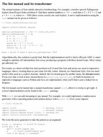
The list monad and its transformerThe monad instance of lists admits attractive backtracking. For example, consider special Pythagoreantriplets from Project Euler problem 9: find three natural numbers a < b < c such that a^2 + b^2 = c^2 anda + b + c = n, where n = 1000 (there exists exactly one such triplet). A naive implementation using thelist monad can be given as follows:

-- file: backtracking-list.hs

import Control.Monad (guard)

special_pythagorean :: Int -> [(Int,Int,Int)]special_pythagorean n = do a <- [1 .. n] b <- [a + 1 .. n] c <- [b + 1 .. n] guard (a + b + c == n) guard (a ^ 2 + b ^ 2 == c ^ 2) return (a, b, c)

main = print $ head $ special_pythagorean 1000

Algorithmically, this solution is pretty bad. But the implementation itself is fairly efficient. GHC is smartenough to optimize all intermediate lists away, producing a program with three nested loops. Most valuesget unboxed, too.

Previously we observed that lists don't perform well if used like lists and arrays are used in imperativelanguages, that is, treating them as just some list-like values. Instead, in a functional style, lists are moreuseful when used as a control structure. Indeed, the list monad goes by another name, the stream monad.If you ever take a look at how stream fusion in bytestring, vector, text, or built-in iterators inimperative languages such as Python and Java are implemented, what you'll find is just a linked list indisguise.

The list monad can be turned into a monad transformer, named ListT, albeit it is tricky to get right. Acorrect implementation can be found in the list-t package.

With ListT, we can add streaming to any monad. For example, we could implement a random noisegenerator with a repeating pattern and random delays with a ListT IO. First, some imports:

-- file: noise.hs

import ListT -- package list-timport System.Random -- package randomimport Control.Monad.Trans (lift) -- package mtlimport Control.Concurrent (threadDelay)

We write the noise generator to take the pattern as an argument:

noise :: [Double] -> ListT IO Doublenoise pat = do pat'<- ListT.repeat pat x <- ListT.fromFoldable pat' lift $ do delay <- randomIO

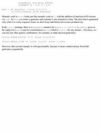
threadDelay (mod delay 300000) randomRIO (x - 0.5, x + 0.5)

main = let generator = noise [1,5,10,5] in ListT.traverse_ print generator

Monadic code in ListT looks just like monadic code in [], with the addition of interleaved IO actionsvia lift. In main, we create a generator and consume it one element at a time. The next item is generatedonly when it is really required, hence we don't loop indefinitely but recurse productively.

In the list-t package, there is a MonadPlus instance for Monad m => ListT m. MonadPlus gives usthe empty list (mzero) and list concatenation (mplus) lifted to ListT m for any monad m. Of course, wecan also use other generic combinators, for example, to make derived generators:

Control.Monad.mfilter (> 5) (noise [1,5,10,5])

Control.Monad.liftM (+) (noise [1,2,3]) (noise [7,6,8])

However, that second example is a bit questionable, because it incurs random delays from bothgenerators sequentially.

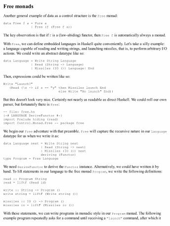
Free monadsAnother general example of data as a control structure is the Free monad:

data Free f a = Pure a | Free (f (Free f a))

The key observation is that if f is a (law-abiding) functor, then Free f is automatically always a monad.

With Free, we can define embedded languages in Haskell quite conveniently. Let's take a silly example:a language capable of reading and writing strings, and launching missiles, that is, to perform arbitrary I/Oactions. We could write an abstract datatype like so:

data Language = Write String Language | Read (String -> Language) | Missiles (IO ()) Language| End

Then, expressions could be written like so:

Write "Launch?" (Read (\s -> if s == "y" then Missiles launch End else Write "No launch" End))

But this doesn't look very nice. Certainly not nearly as readable as direct Haskell. We could roll our ownparser, but fortunately there is Free:

-- file: free.hs{-# LANGUAGE DeriveFunctor #-}import Prelude hiding (read)import Control.Monad.Free -- package free

We begin our Free adventure with that preamble. Free will capture the recursive nature in our Languagedatatype for us when we write it as:

data Language next = Write String next | Read (String -> next) | Missiles (IO ()) next deriving (Functor)type Program = Free Language

We need DeriveFunctor to derive the Functor instance. Alternatively, we could have written it byhand. To lift statements in our language to the free monad Program, we write the following definitions:

read :: Program Stringread = liftF (Read id)

write :: String -> Program ()write string = liftF (Write string ())

missiles :: IO () -> Program ()missiles io = liftF (Missiles io ())

With these statements, we can write programs in monadic style in our Program monad. The followingexample program repeatedly asks for a command until receiving a "launch" command, after which it

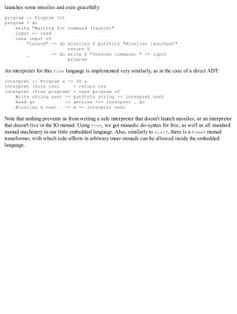
launches some missiles and exits gracefully:

program :: Program Intprogram = do write "Waiting for command (launch)" input <- read case input of "launch" -> do missiles $ putStrLn "Missiles launched!" return 0 _ -> do write $ "Unknown command: " ++ input program

An interpreter for this Free language is implemented very similarly, as in the case of a direct ADT:

interpret :: Program a -> IO ainterpret (Pure res) = return resinterpret (Free program) = case program of Write string next -> putStrLn string >> interpret next Read go -> getLine >>= interpret . go Missiles m next -> m >> interpret next

Note that nothing prevents us from writing a safe interpreter that doesn't launch missiles, or an interpreterthat doesn't live in the IO monad. Using Free, we got monadic do-syntax for free, as well as all standardmonad machinery in our little embedded language. Also, similarly to ListT, there is a FreeT monadtransformer, with which side-effects in arbitrary inner monads can be allowed inside the embeddedlanguage.

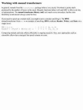
Working with monad transformersIn general, monads from the transformers package behave very nicely. Overhead is pretty muchpredicted by the number of layers in the stack. Monadic functions inline well and GHC is able to do lotsof optimizations. The monad transformer library (mtl) isn't much worse nowadays, but the extraflexibility in mtl doesn't always come for free.

If you need to speed up a monad stack, you might want to consider unrolling it. The RWSmonad/transformer from mtl is an example of unrolling. RWS combines Reader, Writer, and State on asingle level:

RWS r w s a ~ r -> s -> (a, s, w)ReaderT r (StateT s (Writer w)) a ~ r -> s -> ((a, s), w)

Composing monads and side-effects efficiently is ongoing research. Also, new approaches such asextensible effects have emerged, but speed remains an issue.

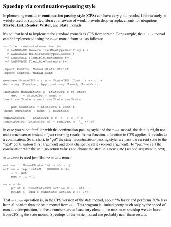
Speedup via continuation-passing styleImplementing monads in continuation-passing style (CPS) can have very good results. Unfortunately, nowidely-used or supported library I'm aware of would provide drop-in replacements for ubiquitousMaybe, List, Reader, Writer, and State monads.

It's not that hard to implement the standard monads in CPS from scratch. For example, the State monadcan be implemented using the Cont monad from mtl as follows:

-- file: cont-state-writer.hs{-# LANGUAGE GeneralizedNewtypeDeriving #-}{-# LANGUAGE MultiParamTypeClasses #-}{-# LANGUAGE FlexibleInstances #-}{-# LANGUAGE FlexibleContexts #-}

import Control.Monad.State.Strictimport Control.Monad.Cont

newtype StateCPS s r a = StateCPS (Cont (s -> r) a)deriving (Functor, Applicative, Monad, MonadCont)

instance MonadState s (StateCPS s r) where get = StateCPS $ cont $\next curState → next curState curState

put newState = StateCPS $ cont $\next curState → next () newState

runStateCPS :: StateCPS s s () -> s -> srunStateCPS (StateCPS m) = runCont m (\_ -> id)

In case you're not familiar with the continuation-passing style and the Cont monad, the details might notmake much sense: instead of just returning results from a function, a function in CPS applies its results toa continuation. So in short, to "get" the state in continuation-passing style, we pass the current state to the"next" continuation (first argument) and don't change the state (second argument). To "put,"we call thecontinuation with the unit (no return value) and change the state to a new state (second argument to next).

StateCPS is used just like the State monad:

action :: MonadState Int m => m ()action = replicateM_ 1000000 $ do i <- get put $! i + 1

main = do print $ (runStateCPS action 0 :: Int) print $ (snd $ runState action 0 :: Int)

That action operation is, in the CPS version of the state monad, about 5% faster and performs 30% lessheap allocation than the state monad from mtl. This program is limited pretty much only by the speed ofmonadic composition, so these numbers are at least very close to the maximum speedup we can havefrom CPSing the state monad. Speedups of the writer monad are probably near these results.

Other standard monads can be implemented similarly to StateCPS. The definitions can also begeneralized to monad transformers over an arbitrary monad (a la ContT). For extra speed, you mightwish to combine many monads in a single CPS monad, similarly to what RWST does.

SummaryWe began this chapter with GHC primitives such as Int# and figured out the effects of strictness andunpacking annotations (bangs and UNPACK-pragmas) in data type definitions. We noted that tuples arelazy and that Bool is an algebraic data type, but we also noted that arrays and vectors represent Boolintelligently as single bits internally.

Then we considered working with numeric, binary, and textual data. We witnessed the performance of thebytestring, text, and vector libraries, all of which get their speed from fusion optimizations, incontrast to linked lists, which have a huge overhead despite also being subject to fusion to some degree.However, linked lists give rise to simple difference lists and zippers. The builder patterns for lists,bytestring, and text were introduced. We discovered that the array package is low-level and clumsycompared to the superior vector package, unless you must support Haskell 98. The Map type incontainers was a binary tree, whereas some hashing-based (functional) implementations resided inunordered containers. We used the IO and ST monads to program with mutable state. Finally, we touchedupon the subject of side-effect composition.

In the next chapter, we will profile and benchmark Haskell code using the GHC profiler and criterion.Our aim is to identify space leaks and cost centers. We will learn how to structure and annotate programsfor easy profiling.

Chapter 3. Profile and Benchmark to Your Heart's ContentSo far we haven't used much else but heap usage statistics to gauge the performance of Haskell programs.For a quick overview of the overall performance of a program, a simple +RTS -s is often sufficient.However, often it is necessary to know which parts of the code specifically are taking up the most timeand space.

In this chapter we extend our toolset with more sophisticated profiling and benchmarking facilities. Wewill learn to inspect and set cost centres, to benchmark robustly when semantics are mostly lazy. Finallywe'll also look at monitoring performance while the program is still running.

Profiling time, allocation and space usageProfiling the heap: break-downs and subset selectionBenchmarking Haskell programs with the criterion libraryMonitoring still-executing programs in real-time with ekg

Profiling time and allocationsProfiling in the presence of lazy evaluation does not differ much from profiling always-strict programs.The profiler that comes with GHC assigns time and space usages to cost centres. Cost centres annotateexpressions, and can be set either manually or automatically by GHC. Cost centres can occur enclosed inother cost centres recursively, forming cost centre stacks. All time and space costs accumulate in eachenclosing cost centre.

Cost centres can be set manually via annotations, or automatically by GHC via compiler flags.Depending on how often the cost centre is entered, the choice of cost centre can have a big impact onoverall execution time. Fortunately, allocation profiling is not affected by chosen cost centers.

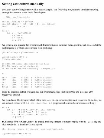
Setting cost centres manuallyLet's start our profiling journey with a basic example. The following program uses the simple movingaverage function we wrote in the first chapter:

-- file: prof-basics.hs

sma :: [Double] -> [Double]sma (x0:x1:xs) = (x0 + x1) / 2 : sma (x1:xs)sma xs = xs

main = let a = [1..1000000] b = sma a c = sum b in print c

We compile and execute this program with Runtime System statistics but no profiling yet, to see what theperformance is without any overhead from profiling:

ghc -O -rtsopts prof-basics.hs

./prof-basics +RTS -s5.000009999995e11

264,106,248 bytes allocated in the heap255,768 bytes copied during GC44,312 bytes maximum residency (2 sample(s))

...

INIT time 0.000s ( 0.000s elapsed)MUT time 0.105s ( 0.105s elapsed)GC time 0.002s ( 0.002s elapsed)EXIT time 0.000s ( 0.000s elapsed)Total time 0.111s ( 0.108s elapsed)

From the statistics output, we learn that our program executes in about 110ms and allocates 260Megabytes of heap.

We would now like to know which of the parts a, b, or c is consuming the most resources. To do this, wecan set cost centres with {-# SCC identifier #-} pragmas and so modify our main accordingly:

main = let a = {-# SCC "list-" #-} [1..1000000] b = {-# SCC "sma-" #-} sma a c = {-# SCC "sum-" #-} sum b in print c

SCC stands for Set Cost Centre. To enable profiling support, we must compile with the -prof flag andalso enable the -p Runtime System option:

ghc -fforce-recomp -O -rtsopts -prof prof-basics.hs

./prof-basics +RTS -s -p

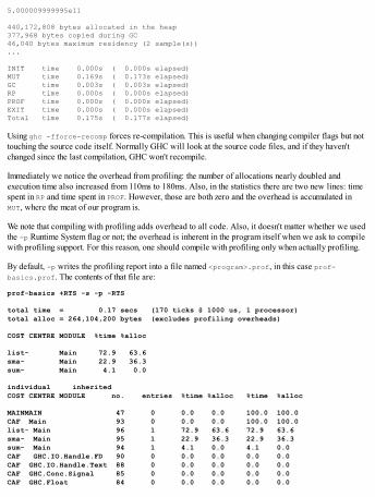
5.000009999995e11

440,172,808 bytes allocated in the heap377,968 bytes copied during GC46,040 bytes maximum residency (2 sample(s))...

INIT time 0.000s ( 0.000s elapsed)MUT time 0.169s ( 0.173s elapsed)GC time 0.003s ( 0.003s elapsed)RP time 0.000s ( 0.000s elapsed)PROF time 0.000s ( 0.000s elapsed)EXIT time 0.000s ( 0.000s elapsed)Total time 0.175s ( 0.177s elapsed)

Using ghc -fforce-recomp forces re-compilation. This is useful when changing compiler flags but nottouching the source code itself. Normally GHC will look at the source code files, and if they haven'tchanged since the last compilation, GHC won't recompile.

Immediately we notice the overhead from profiling: the number of allocations nearly doubled andexecution time also increased from 110ms to 180ms. Also, in the statistics there are two new lines: timespent in RP and time spent in PROF. However, those are both zero and the overhead is accumulated inMUT, where the meat of our program is.

We note that compiling with profiling adds overhead to all code. Also, it doesn't matter whether we usedthe -p Runtime System flag or not; the overhead is inherent in the program itself when we ask to compilewith profiling support. For this reason, one should compile with profiling only when actually profiling.

By default, -p writes the profiling report into a file named <program>.prof, in this case prof-basics.prof. The contents of that file are:

prof-basics +RTS -s -p -RTS

total time = 0.17 secs (170 ticks @ 1000 us, 1 processor)total alloc = 264,104,200 bytes (excludes profiling overheads)

COST CENTRE MODULE %time %alloc

list- Main 72.9 63.6sma- Main 22.9 36.3sum- Main 4.1 0.0

individual inheritedCOST CENTRE MODULE no. entries %time %alloc %time %alloc

MAINMAIN 47 0 0.0 0.0 100.0 100.0CAF Main 93 0 0.0 0.0 100.0 100.0list- Main 96 1 72.9 63.6 72.9 63.6sma- Main 95 1 22.9 36.3 22.9 36.3sum- Main 94 1 4.1 0.0 4.1 0.0CAF GHC.IO.Handle.FD 90 0 0.0 0.0 0.0 0.0CAF GHC.IO.Handle.Text 88 0 0.0 0.0 0.0 0.0CAF GHC.Conc.Signal 85 0 0.0 0.0 0.0 0.0CAF GHC.Float 84 0 0.0 0.0 0.0 0.0

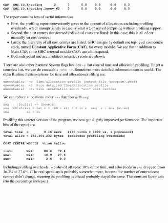
CAF GHC.IO.Encoding 2 0 0.0 0.0 0.0 0.0CAF GHC.IO.Encoding.Iconv 62 0 0.0 0.0 0.0 0.0

The report contains lots of useful information:

First, the profiling report conveniently gives us the amount of allocations excluding profilingoverheads, which unsurprisingly is exactly what we observed compiling without profiling support.Second, the cost centres that accrued individual costs are listed. In this case, this is all of ourmanually set cost centres.Lastly, the hierarchy of all cost centres are listed. GHC assigns by default one top-level cost centrestack, named Constant Applicative Form (CAF), for every module. We see that in addition toMain.CAF, some GHC-internal module CAFs are also exposed.Both individual and accumulated (inherited) costs are shown.

There are also other Runtime System flags besides -p that control time and allocation profiling. To get acomplete list, we can do executable +RTS -?. Sometimes more detailed information can be useful. Theextra Runtime System options for time and allocation profiling are:

executable: -p Time/allocation profile (output file <program>.prof)executable: -P More detailed Time/Allocation profileexecutable: -Pa Give information about *all* cost centres

We can reduce allocations in our sma function with seq:

sma :: [Double] -> [Double]sma (x0:x1:xs) = let r = (x0 + x1) / 2 in r `seq` r : sma (x1:xs)sma xs = xs

Profiling this stricter version of the program, we now get slightly improved performance. The importantbits of the report are:

total time = 0.16 secs (160 ticks @ 1000 us, 1 processor)total alloc = 232,104,232 bytes (excludes profiling overheads)

COST CENTRE MODULE %time %alloc

list- Main 80.6 72.4sma- Main 16.9 27.6sum- Main 2.5 0.0

Including profiling overheads, we shaved off some 10% of the time, and allocations in sma dropped from36.3% to 27.6%. (The real speed-up is probably somewhat more, because the number of entered costcentres didn't change, meaning the profiling overhead probably stayed the same. That constant factor eatsinto the percentage increase.)

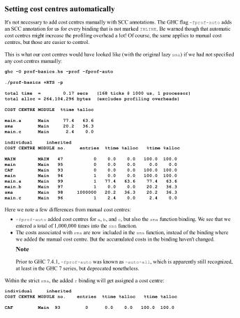
Setting cost centres automaticallyIt's not necessary to add cost centres manually with SCC annotations. The GHC flag -fprof-auto addsan SCC annotation for us for every binding that is not marked INLINE. Be warned though that automaticcost centres might increase the profiling overhead a lot! Of course, the same applies to manual costcentres, but those are easier to control.

This is what our cost centres would have looked like (with the original lazy sma) if we had not specifiedany cost centres manually:

ghc -O prof-basics.hs -prof -fprof-auto

./prof-basics +RTS -p

total time = 0.17 secs (168 ticks @ 1000 us, 1 processor)total alloc = 264,104,296 bytes (excludes profiling overheads)

COST CENTRE MODULE %time %alloc

main.a Main 77.4 63.6sma Main 20.2 36.3main.c Main 2.4 0.0

individual inheritedCOST CENTRE MODULE no. entries %time %alloc %time %alloc

MAIN MAIN 47 0 0.0 0.0 100.0 100.0main Main 95 0 0.0 0.0 0.0 0.0CAF Main 93 0 0.0 0.0 100.0 100.0main Main 94 1 0.0 0.0 100.0 100.0main.a Main 99 1 77.4 63.6 77.4 63.6main.b Main 97 1 0.0 0.0 20.2 36.3sma Main 98 1000000 20.2 36.3 20.2 36.3main.c Main 96 1 2.4 0.0 2.4 0.0

Here we note a few differences from manual cost centres:

-fprof-auto added cost centres for a, b, and c, but also the sma function binding. We see that weentered a total of 1,000,000 times into the sma function.The costs associated with sma are now included in the sma function, instead of the binding wherewe added the manual cost centre. But the accumulated costs in the binding haven't changed.

Note

Prior to GHC 7.4.1, -fprof-auto was known as -auto-all, which is apparently still recognized,at least in the GHC 7 series, but deprecated nonetheless.

Within the strict sma, the added r binding will get assigned a cost centre:

individual inheritedCOST CENTRE MODULE no. entries %time %alloc %time %alloc

CAF Main 93 0 0.0 0.0 100.0 100.0

main Main 94 1 0.0 0.0 100.0 100.0main.a Main 99 1 69.4 72.4 69.4 72.4main.b Main 97 1 0.0 0.0 27.1 27.6sma Main 98 1000000 26.5 27.6 27.1 27.6sma.r Main 100 999999 0.6 0.0 0.6 0.0main.c Main 96 1 3.5 0.0 3.5 0.0

That new cost centre adds so much overhead when invoked a million times that time-wise we don't seeany improvement over the lazy version when compiled with profiling. However, allocations aren'taffected.

What if we had both automatic and manual cost centres for the a, b, and c bindings? The profilingoverhead would have increased even more. In fact, it would have increased so much that the strictversion is 10% slower than the lazy one when profiling!

The takeaway here is that not much can be deduced from profiling just time. Allocation profiling is morevaluable because profiling doesn't interfere with the amount of allocations done (apart from doing itsown allocation and subsequently subtracting those in the report).

With -O and higher, GHC routinely lifts constant expressions to the toplevel, but this is not normallyreflected in the cost centre stack. With the -fprof-cafs flag, we ask GHC to assign individual costcentres to CAFs lifted to the toplevel. The upside of -fprof-cafs is that the profiling report then moreclosely resembles the real structure of the program, the cost centre stacks don't get so deep, and profilingoverheads reduce. The downside is that one might need to take a look at the Core (obtained via -ddump-simple) in order to figure out what the lifted CAFs correspond to.

Installing libraries with profilingProfiling programs that depend on extra modules requires that those modules were built with profilingsupport. The libraries that come with Haskell Platform have been built with profiling. Some distributionshave enabled profiling in their Haskell packages and some provide the profiling libraries in separatepackages.

Haskell libraries that you have installed via cabal-install, or stack, do not in general have profilingenabled. To profile code that uses such libraries, it is necessary to re-install them with profiling. One canalso create a cabal sandbox, which we will not cover here.

Enabling profiling for dependencies using stack is easy:

stack build --executable-profiling –-library-profiling

Stack conveniently re-builds all necessary packages that didn't previously have profiling enabled.

Using cabal-install re-installs is more tedious. The fastest and most straightforward way is to enablelibrary-profiling: True in your ~/.cabal/config, remove ~/.ghc, and then install packages youwant to use.

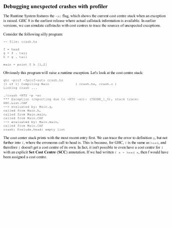
Debugging unexpected crashes with profilerThe Runtime System features the -xc flag, which shows the current cost centre stack when an exceptionis raised. GHC 8 is the earliest release where actual callstack information is available. In earlierversions, we can simulate callstacks with cost centres to trace the sources of unexpected exceptions.

Consider the following silly program:

-- file: crash.hs

f = headg = f . tailh = g . tail

main = print $ h [1,2]

Obviously this program will raise a runtime exception. Let's look at the cost centre stack:

ghc -prof -fprof-auto crash.hs[1 of 1] Compiling Main ( crash.hs, crash.o )Linking crash ...

./crash +RTS -p -xc*** Exception (reporting due to +RTS -xc): (THUNK_1_0), stack trace:GHC.List.CAF--> evaluated by: Main.g,called from Main.h,called from Main.main,called from Main.CAF--> evaluated by: Main.main,called from Main.CAFcrash: Prelude.head: empty list

The cost center stack prints with the most recent entry first. We can trace the error to definition g, but notfurther into f, where the erroneous call to head is. This is because, for GHC, f is the same as head, andtherefore f doesn't get a cost centre of its own. In fact, it isn't possible to even have a cost centre for fwith an explicit Set Cost Centre (SCC) annotation. If we had written f x = head x, then f would havebeen assigned a cost centre.

Heap profilingFrom the profiling report (+RTS -p) we were able to infer how much different cost centres allocatedspace, along with a rough estimate of time spent in cost centres in total during the program's lifetime.What if we wanted to see how space usage varies across that lifetime? That would be useful to pinpointspace leaks that manifest themselves only at certain events.

GHC includes a heap profiler, which put simply snapshots heap usage at small fixed intervals andgenerates a time-dependent report in the form of a .hp file. To enable the heap profiler for an executable,the same -prof flag for GHC is enough. Some limited heap profiling is also supported when compiledwithout profiling. The same cost centres used for time and allocation profiling are also used for heapprofiling, if the heap profile is generated or narrowed down based on cost centres.

To extract a heap report, we need to use some of the -h family of Runtime System options. Those optionsare as follows:

-h<break-down> Heap residency profile (hp2ps) (output file <program>.hp) break-down: c = cost centre stack (default) m = module d = closure description y = type description r = retainer b = biography (LAG,DRAG,VOID,USE)

A subset of closures may be selected thusly:

-hc<cc>,... specific cost centre(s) (top of stack only)-hC<cc>,... specific cost centre(s) (anywhere in stack)-hm<mod>... all cost centres from the specified modules(s)-hd<des>,... closures with specified closure descriptions-hy<typ>... closures with specified type descriptions-hr<cc>... closures with specified retainers-hb<bio>... closures with specified biographies (lag,drag,void,use)

This help message is quite dense. Basically, there are two separate concepts: break-down and closuresubset selection.

The break-down subset defines the kinds of thing we associate heap residencies with. That is, the spacetaken by heap objects is accumulated in one of the following:

cost centres (-hc): Pin-point heap residency to automatic or manual (SCC) cost centers.per-module (-hm): Pin-point residency to Haskell modules.closure descriptions (-hd): Constructors and GHC internals.Type description (-hy): Types such as Double, String, Maybe, and so on. Unknown andpolymorphic types are given some approximation.Retainers (-hr): We'll discuss retainers shortly.Biography (-hb): The state a heap object is in, also discussed later.

The usual strategy is to break the heap profile down by cost centres (-hc). The complementary concept toheap break-down is closure subsets. By restricting profiling to some subsets of closures, we can narrowdown the parts of the program we are actually interested in. The same options apply for subset selection

as for break-down.

There can be only one break-down option, but multiple closure subset selections. With break-down, wechoose the level at which we wish to inspect the program; with closure subsets, we define the parts of theprogram we are interested in.

For example, this combination will generate a heap profile broken down by cost centres in the Mainmodule of all values of type Double:

+RTS -hc -hmMain -hyDouble

You can also compile without profiling and still use the -h Runtime System option, at least with a recentGHC. This eliminates the profiling overhead, leaving only minimal overhead from taking residencysamples from the heap, but then the profiler options are limited to a -h only. When profiling is disabled,a -h (long form -hT) is pretty much identical to -hd when profiling is enabled.

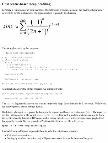
Cost centre-based heap profilingLet's take a real example of heap profiling. The following program calculates the Taylor polynomial ofdegree 800 for the sin function. The approximation is given by this formula:

This is implemented by this program:

-- file: heap-profiling.hs

sin' :: Double -> Doublesin' x = go 0 x where go n x | n > precision = x | otherwise = go (n + 1) $ x + (-1) ** n * x ** (2 * n + 1) / factorial (2 * n + 1)

precision = 800

factorial n = product [1..n]

main = print $ sum $ map sin' [0,0.1..1]

To extract a heap profile of this program, we compile it with:

ghc -rtsopts -prof -fprof-auto heap-profiling.hs

./heap-profiling +RTS -hc -i0.05

The -i0.05 flag sets the interval we want to sample the heap. By default, this is 0.1 seconds. We halve itfor our program to extract enough details.

By default, when just -h is given, the heap profile is generated based on cost centres (-hc). The report iswritten in this case to a file named heap-profiling.hp. It is hard to deduce anything meaningful fromthe .hp file directly. Instead, GHC comes with a binary called hp2ps, which produces nice graphs fromheap profile reports. We can generate a PostScript file from a .hp file with hp2ps:

hp2ps -c -d -e8in heap-profiling.hp

I included some additional arguments there to make the output more readable:

Colorized output with -cSorting by standard deviation (-d) will push more static bars to the bottom of the graph

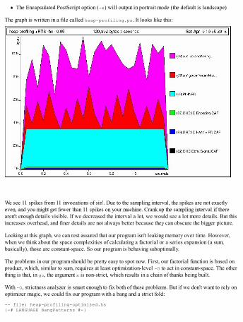
The Encapsulated PostScript option (-e) will output in portrait mode (the default is landscape)

The graph is written in a file called heap-profiling.ps. It looks like this:

We see 11 spikes from 11 invocations of sin'. Due to the sampling interval, the spikes are not exactlyeven, and you might get fewer than 11 spikes on your machine. Crank up the sampling interval if therearen't enough details visible. If we decreased the interval a lot, we would see a lot more details. But thisincreases overhead, and finer details are not always better because they can obscure the bigger picture.

Looking at this graph, we can rest assured that our program isn't leaking memory over time. However,when we think about the space complexities of calculating a factorial or a series expansion (a sum,basically), those are constant-space. So our program is behaving suboptimally.

The problems in our program should be pretty easy to spot now. First, our factorial function is based onproduct, which, similar to sum, requires at least optimization-level -O to act in constant-space. The otherthing is that, in go, the argument x is non-strict, which results in a chain of thunks being built.

With -O, strictness analyzer is smart enough to fix both of these problems. But if we don't want to rely onoptimizer magic, we could fix our program with a bang and a strict fold:

-- file: heap-profiling-optimized.hs{-# LANGUAGE BangPatterns #-}

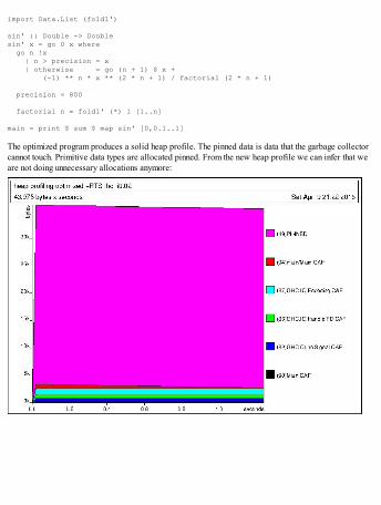
import Data.List (foldl')

sin' :: Double -> Doublesin' x = go 0 x where go n !x | n > precision = x | otherwise = go (n + 1) $ x + (-1) ** n * x ** (2 * n + 1) / factorial (2 * n + 1)

precision = 800

factorial n = foldl' (*) 1 [1..n]

main = print $ sum $ map sin' [0,0.1..1]

The optimized program produces a solid heap profile. The pinned data is data that the garbage collectorcannot touch. Primitive data types are allocated pinned. From the new heap profile we can infer that weare not doing unnecessary allocations anymore:

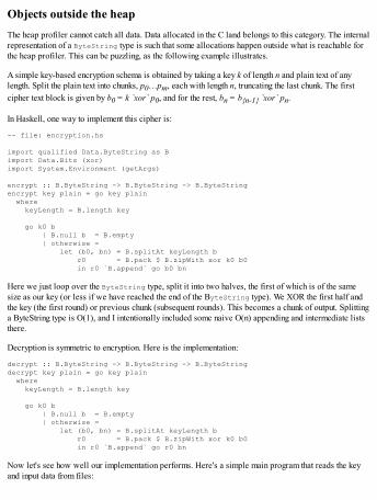
Objects outside the heapThe heap profiler cannot catch all data. Data allocated in the C land belongs to this category. The internalrepresentation of a ByteString type is such that some allocations happen outside what is reachable forthe heap profiler. This can be puzzling, as the following example illustrates.

A simple key-based encryption schema is obtained by taking a key k of length n and plain text of anylength. Split the plain text into chunks, p0…pm, each with length n, truncating the last chunk. The firstcipher text block is given by b0 = k `xor` p0, and for the rest, bn = b{n-1} `xor` pn.

In Haskell, one way to implement this cipher is:

-- file: encryption.hs

import qualified Data.ByteString as Bimport Data.Bits (xor)import System.Environment (getArgs)

encrypt :: B.ByteString -> B.ByteString -> B.ByteStringencrypt key plain = go key plain where keyLength = B.length key

go k0 b | B.null b = B.empty | otherwise = let (b0, bn) = B.splitAt keyLength b r0 = B.pack $ B.zipWith xor k0 b0 in r0 `B.append` go b0 bn

Here we just loop over the ByteString type, split it into two halves, the first of which is of the samesize as our key (or less if we have reached the end of the ByteString type). We XOR the first half andthe key (the first round) or previous chunk (subsequent rounds). This becomes a chunk of output. Splittinga ByteString type is O(1), and I intentionally included some naive O(n) appending and intermediate liststhere.

Decryption is symmetric to encryption. Here is the implementation:

decrypt :: B.ByteString -> B.ByteString -> B.ByteStringdecrypt key plain = go key plain where keyLength = B.length key

go k0 b | B.null b = B.empty | otherwise = let (b0, bn) = B.splitAt keyLength b r0 = B.pack $ B.zipWith xor k0 b0 in r0 `B.append` go r0 bn

Now let's see how well our implementation performs. Here's a simple main program that reads the keyand input data from files:

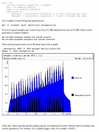
main = do [action, keyFile, inputFile] <- getArgs key <- B.readFile keyFile input <- B.readFile inputFile case action of "encrypt" -> B.writeFile (inputFile ++ ".out") $ encrypt key input "decrypt" -> B.writeFile (inputFile ++ ".out") $ decrypt key input

Let's compile with profiling and optimizations:

ghc -O -rtsopts -prof -fprof-auto encryption.hs

To test at a good enough scale, I used a key size of 1 MB and plain text size of 24 MB. Those can begenerated as random samples:

dd if=/dev/urandom of=key.bin bs=1M count=1dd if=/dev/urandom of=plain.bin bs=1M count=24

Then run the program and convert the heap report into a graph:

./encryption +RTS -h -RTS encrypt key.bin plain.binhp2ps -c -e8in encryption.hp

(Note that, when reproducing this graph yourself, you might need to play with the interval setting to getsimilar granularity. For instance, try a slightly bigger value, for example -i0.005.)

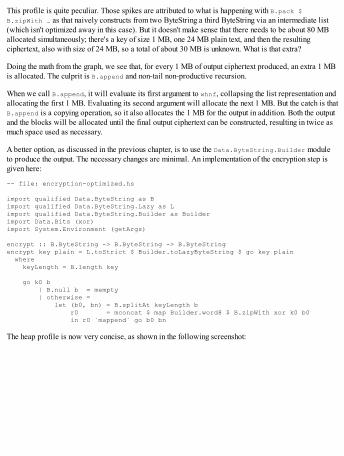
This profile is quite peculiar. Those spikes are attributed to what is happening with B.pack $B.zipWith … as that naively constructs from two ByteString a third ByteString via an intermediate list(which isn't optimized away in this case). But it doesn't make sense that there needs to be about 80 MBallocated simultaneously; there's a key of size 1 MB, one 24 MB plain text, and then the resultingciphertext, also with size of 24 MB, so a total of about 30 MB is unknown. What is that extra?

Doing the math from the graph, we see that, for every 1 MB of output ciphertext produced, an extra 1 MBis allocated. The culprit is B.append and non-tail non-productive recursion.

When we call B.append, it will evaluate its first argument to whnf, collapsing the list representation andallocating the first 1 MB. Evaluating its second argument will allocate the next 1 MB. But the catch is thatB.append is a copying operation, so it also allocates the 1 MB for the output in addition. Both the outputand the blocks will be allocated until the final output ciphertext can be constructed, resulting in twice asmuch space used as necessary.

A better option, as discussed in the previous chapter, is to use the Data.ByteString.Builder moduleto produce the output. The necessary changes are minimal. An implementation of the encryption step isgiven here:

-- file: encryption-optimized.hs

import qualified Data.ByteString as Bimport qualified Data.ByteString.Lazy as Limport qualified Data.ByteString.Builder as Builderimport Data.Bits (xor)import System.Environment (getArgs)

encrypt :: B.ByteString -> B.ByteString -> B.ByteStringencrypt key plain = L.toStrict $ Builder.toLazyByteString $ go key plain where keyLength = B.length key

go k0 b | B.null b = mempty | otherwise = let (b0, bn) = B.splitAt keyLength b r0 = mconcat $ map Builder.word8 $ B.zipWith xor k0 b0 in r0 `mappend` go b0 bn

The heap profile is now very concise, as shown in the following screenshot:

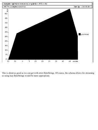
This is about as good as we can get with strict ByteStrings. Of course, the schema allows for streamingso using lazy ByteStrings would be more appropriate.

Retainer profilingRetainer profiling (+RTS -hr) is designed to help track down space leaks. The retainer profiler breaksdown the heap by retainer sets. The system stack, thunks, and explicitly mutable objects are retainers. Alllive objects are retained by one or more retainer objects.

Let's take an example:

let xs = [1..100000] a = sum xs

Here a is a retainer for xs. xs is not yet nothing but an unevaluated, cheap thunk (as is a). If we asked forlength xs, forcing the evaluation of xs, then xs becomes a large evaluated structure in the heap, which isretained by a. The retainer profiler spots such retaining and reports a as a retainer for a lot of data. Ofcourse, if we evaluated a to WHNF, then it would stop being a retainer, because constructors are notretainers.

Let's take another illustratives example and actually do some retainer profiling. The following performstwo calculations on two distinct lists:

-- file: mean.hs

mean xs = sum xs / fromIntegral (length xs)

sumlg xs = sum (map log xs)

main = do print $ mean [1..1000000] print $ sumlg [1..1000001]

Asking for a retainer profiling, we need to compile with profiling, execute with the Runtime System flag-hr, and finally generate a graph from the heap profile:

ghc -rtsopts -prof -fprof-auto mean.hs./mean +RTS -hr -i0.02hp2ps -e8in -c mean.hp

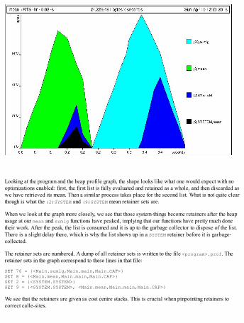
Looking at the program and the heap profile graph, the shape looks like what one would expect with nooptimizations enabled: first, the first list is fully evaluated and retained as a whole, and then discarded aswe have retrieved its mean. Then a similar process takes place for the second list. What is not quite clearthough is what the (2)SYSTEM and (9)SYSTEM mean retainer sets are.

When we look at the graph more closely, we see that those system-things become retainers after the heapusage at our mean and sumlg functions have peaked, implying that our functions have pretty much donetheir work. After the peak, the list is consumed and it is up to the garbage collector to dispose of the list.There is a slight delay there, which is why the list shows up in a SYSTEM retainer before it is garbage-collected.

The retainer sets are numbered. A dump of all retainer sets is written to the file <program>.prof. Theretainer sets in the graph correspond to these lines in that file:

SET 76 = {<Main.sumlg,Main.main,Main.CAF>}SET 8 = {<Main.mean,Main.main,Main.CAF>}SET 2 = {<SYSTEM.SYSTEM>}SET 9 = {<SYSTEM.SYSTEM>, <Main.mean,Main.main,Main.CAF>}

We see that the retainers are given as cost centre stacks. This is crucial when pinpointing retainers tocorrect calle-sites.

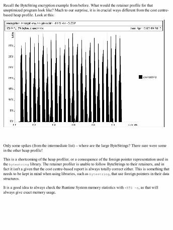
Recall the ByteString encryption example from before. What would the retainer profile for thatunoptimized program look like? Much to our surprise, it is in crucial ways different from the cost centre-based heap profile. Look at this:

Only some spikes (from the intermediate list) – where are the large ByteStrings? There sure were somein the other heap profile!

This is a shortcoming of the heap profiler, or a consequence of the foreign pointer representation used inthe bytestring library. The retainer profiler is unable to follow ByteStrings to their retainers, and infact it isn't a given that the cost centre-based report is always totally correct either. This is something thatneeds to be kept in mind when using libraries, such as bytestring, that use foreign pointers in their datastructures.

It is a good idea to always check the Runtime System memory statistics with +RTS -s, as that willalways give exact memory usage.

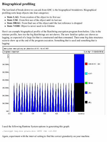
Biographical profilingThe last kind of break-down we can ask from GHC is the biographical breakdown. Biographicalprofiling sorts heap objects into four categories:

State LAG: From creation of the object to its first useState USE: From first use of the object until its last useState DRAG: From final use of the object until the last reference is droppedState VOID: Object is never used in its lifetime

Here's an example biographical profile of the ByteString encryption program from before. Like in theretainer profile, here too the big ByteStrings are not shown. The now familiar spikes are shown aslagging, as expected of a large list that is constructed and then consumed. Then some big data structuresseem to show up at the end of the program execution. Something that is used and something that islagging:

I used the following Runtime System options in generating this graph:

./encrypt key.bin plain.bin +RTS -hb -i0.002

Again, experiment with the interval setting to find the correct granularity on your machine.

Looking at this graph, it's hard to say much about anything. A more useful use case for biographicalprofiling is to use biographical data in the subset selection, and break-down using some other criteria,such as cost centres.

A usual example would be to find cost centres that produce heap objects in DRAG or VOID states. Thisis achieved with:

program +RTS -hc -hbdrag,void

Then we could find retainers for those cost centres with the +RTS -hr -hccc1,cc2, and so on program.Note that GHC cannot currently do both biographical and retainer profiling simultaneously, so +RTS -hr-hbdrag,void is unfortunately not allowed.

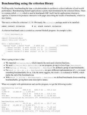
Benchmarking using the criterion libraryProfiling aside, benchmarking the time a calculation takes to perform is a direct indicator of real-worldperformance. Benchmarking Haskell applications is pretty much dominated by the criterion library. Thereis a system called nofib, which is used to benchmark GHC itself, but for applications criterion issuperior. Criterion even produces interactive web pages describing the results of benchmarks, which is anice feature.

This text is written for criterion-1.1.1.0. Obviously, the criterion package needs to be installed:

cabal install criterion # or: stack install criterion

A criterion benchmark suite is created as a normal Haskell program. An example is this:

–– file: benchmark.hs

import Criterion.Mainimport Data.List (foldl')

main = defaultMain [ bgroup "sum" [ bench "sum" $ whnf sum [1..1000000] , bench "foldr" $ whnf (foldr (+) 0) [1..1000000] , bench "foldl" $ whnf (foldl (+) 0) [1..1000000] , bench "foldl'" $ whnf (foldl' (+) 0) [1..1000000] ]]

What is going on here is that:

We imported Criterion.Main, which imports the most used criterion functions.We used Criterion.Main.defaultMain as our program, giving it a list of type [Benchmark].With bgroup :: String → [Benchmark] → Benchmark we defined a group of sum benchmarks.For whnf :: (a → b) → a → Benchmarkable we gave different implementations of sum to createsomething benchmarkable for us. Like the name suggests, the result b is evaluated to WHNF, whichmarks the end of the benchmark run.With bench :: String → Benchmarkable → Benchmark we defined benchmarks from somethingbenchmarkable, giving them some descriptive names.

When we compile with optimizations and run this program, we get the following results:

benchmarking sum/sumtime 309.2 ms (281.0 ms .. 344.2 ms)0.996 R² (0.983 R² .. 1.000 R²)mean 310.4 ms (300.6 ms .. 316.5 ms)std dev 9.535 ms (4.148 ms .. 12.65 ms)variance introduced by outliers: 16% (moderately inflated)

benchmarking sum/foldrtime 66.14 ms (62.61 ms .. 69.17 ms)0.994 R² (0.988 R² .. 0.998 R²)mean 67.27 ms (65.21 ms .. 71.28 ms)std dev 4.686 ms (2.113 ms .. 7.483 ms)variance introduced by outliers: 17% (moderately inflated)

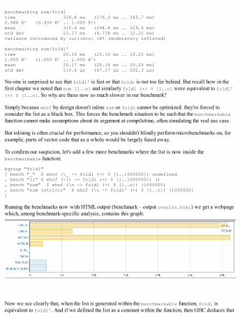
benchmarking sum/foldltime 318.8 ms (276.3 ms .. 365.7 ms)0.988 R² (0.939 R² .. 1.000 R²)mean 315.6 ms (294.8 ms .. 329.6 ms)std dev 23.17 ms (9.738 ms .. 32.22 ms)variance introduced by outliers: 18% (moderately inflated)

benchmarking sum/foldl'time 20.16 ms (20.10 ms .. 20.22 ms)1.000 R² (1.000 R² .. 1.000 R²)mean 20.17 ms (20.14 ms .. 20.25 ms)std dev 110.4 μs (47.27 μs .. 202.3 μs)

No-one is surprised to see that foldl' is fast or that foldr is not too far behind. But recall how in thefirst chapter we noted that sum [1..n] and similarly foldl (+) 0 [1..n] were equivalent to foldl'(+) 0 [1..n]. So why are these now so much slower in our benchmark?

Simply because whnf by design doesn't inline sum or foldl cannot be optimized: they're forced toconsider the list as a black box. This forces the benchmark situation to be such that the benchmarkablefunction cannot make assumptions about its argument at compiletime, often simulating the real use case.

But inlining is often crucial for performance, so you shouldn't blindly perform microbenchmarks on, forexample, parts of vector code that as a whole would be largely fused away.

To confirm our suspicion, let's add a few more benchmarks where the list is now inside thebenchmarkable function:

bgroup "foldl"[ bench "_" $ whnf (\_ -> foldl (+) 0 [1..1000000]) undefined, bench "()" $ whnf (\() -> foldl (+) 0 [1..1000000]) (), bench "num" $ whnf (\n -> foldl (+) 0 [1..n]) (1000000), bench "num (strict)" $ whnf (\n -> foldl' (+) 0 [1..n]) (1000000)]

Running the benchmarks now with HTML output (benchmark – output results.html) we get a webpagewhich, among benchmark-specific analysis, contains this graph:

Now we see clearly that, when the list is generated within the benchmarkable function, foldl isequivalent to foldl'. And if we defined the list as a constant within the function, then GHC deduces that

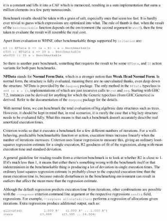
it is a constant and lifts it into a CAF which is memoized, resulting in a sum implementation that sums amillion elements in a few petty nanoseconds.

Benchmark results should be taken with a grain of salt, especially ones that seem too fast. It is hardlyever trivial to guess which expressions are optimized into what. The rule of thumb is that, when the resultof the benchmarkable function depends on the environment (the second argument to whnf), then the timetaken to evaluate the result will resemble the real cost.

Apart from evaluation to WHNF, other benchmarkable things supported by criterion are:

nf :: NFData b => (a → b) → a → BecnhmarkablenfIO :: NFData a => IO a → BenchmarkablewhnfIO :: IO a → Benchmarkable

So there is another pure benchmark, something that requires the result to be some NFData, and IO actionvariants for both pure benchmarks.

NFData stands for Normal Form Data, which is a stronger notion than Weak Head Normal Form. Innormal form, the structure is fully evaluated, meaning there are no unevaluated thunks, even deep downthe structure. NFData is provided by the deepseq package. The only method in the NFData typeclass isrnf :: a → (), implementations of which are just recursive calls to rnf and seq. Starting with GHC7.2, instances can be derived for anything for which the Generic typeclass (from GHC.Generics) isderived. Refer to the documentation of the deepseq package for the details.

With normal form, we can benchmark the total evaluation of big algebraic data structures such as trees.However, it should be kept in mind that, in real scenarios, it is rarely the case that a big lazy structureneeds to be evaluated fully. What this means is that such a benchmark doesn't accurately describe realamortized execution times.

Criterion works so that it executes a benchmark for a few different numbers of iterations. For a well-behaving, predictable benchmarkable function or action, execution times increase linearly when thenumber of iterations increases. Criterion uses linear regression to measure this, giving an ordinary least-squares regression estimate for a single execution, R2 goodness-of-fit of the regression, along with meanexecution time and standard deviation.

A general guideline for reading results from a criterion benchmark is to look at whether R2 is close to 1.If it's much less than 1, it means that either there's something wrong with the benchmark itself or thatindeterminism in the benchmarkable thing is producing a lot of deviation in single execution times. Theordinary least squares regression estimate is probably closer to the expected execution time than themean execution time is, because outside disturbances in the benchmarking environment can result inoutliers that affect the mean more than the regression estimate.

Although the default regression predicts execution time from iterations, other combinations are possiblewith the --regress criterion command line argument or the respective regressions config field,regressions. For example, --regress allocated:iters performs a regression of allocations giveniterations. Extra regressions produce additional output, such as:

allocated: 1.000 R² (1.000 R² .. 1.000 R²)iters 23.999 (23.995 .. 24.004)

y 275.081 (-20091.728 .. 19504.093)

Another R2 goodness-of-fit is given for the regression, along with the slope and y-intercept of the fittedline. Like many other regression metrics, measuring allocations from within the program requiresenabling the Runtime System parameter +RTS -T. Refer to the criterion documentation to learn aboutother available regression metrics.

The criterion library is designed such that it should be relatively easy to adapt it to cover wildly differentuse cases. All necessary datatypes and utility functions are exported and all exported identifiers areextensively documented. JUnit-style reporting is also supported.

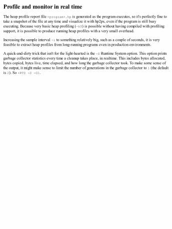
Profile and monitor in real timeThe heap profile report file <program>.hp is generated as the program executes, so it's perfectly fine totake a snapshot of the file at any time and visualize it with hp2ps, even if the program is still busyexecuting. Because very basic heap profiling (-hT) is possible without having compiled with profilingsupport, it is possible to produce running heap profiles with a very small overhead.

Increasing the sample interval -i to something relatively big, such as a couple of seconds, it is veryfeasible to extract heap profiles from long-running programs even in production environments.

A quick-and-dirty trick that isn't for the light-hearted is the -S Runtime System option. This option printsgarbage collector statistics every time a cleanup takes place, in realtime. This includes bytes allocated,bytes copied, bytes live, time elapsed, and how long the garbage collector took. To make some sense ofthe output, it might make sense to limit the number of generations in the garbage collector to 1 (the defaultis 2). So +RTS -S -G1.

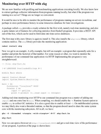
Monitoring over HTTP with ekgWe are now familiar with profiling and benchmarking applications executing locally. We also know howto extract garbage collector information from programs running locally, but what if the program wasrunning on a server? Things are no longer so convenient.

It would be nice to be able to monitor the performance of programs running on servers in realtime, andperhaps to store performance history in some timeseries database for later investigations.

A package called ekg provides a ready solution for the first wish, namely real-time monitoring, and alsoa quite mature set of features for collecting statistics from Haskell programs. It provides a REST APIout-of-the-box, which can be used to fetch data into time-series databases.

The first step with a new library is again to install it. This also installs the ekg-core library, whichcontains metrics. The ekg library provides the monitoring application:

cabal install ekg

Now we get to an example. A silly example, but still an example: a program that repeatedly asks for anumber and prints the factorial of that number. For some reason or other, we want to monitor theperformance of our command-line application via HTTP. Implementing this program is verystraightforward:

-- file: ekg-fact.hs

{-# LANGUAGE OverloadedStrings #-}

module Main where

import Control.Monadimport System.Remote.Monitoring

main = do forkServer "localhost" 8000 forever $ do input <- getLine print $ product [1..read input :: Integer]

Adding real-time monitoring over HTTP to our command-line program was a matter of adding oneimport and one extra line in main. When compiling, we should enable the -T Runtime System option toenable ekg to collect GC statistics. It is also a good idea to enable at least -O. On multithreaded systems,we may likely also want a threaded runtime, so that the program doesn't need to share the same systemcore with the monitoring subsystem. All in all, we have:

ghc -O -threaded -rtsopts -with-rtsopts='-N-T' ekg-fact.hs

ekg-fact

Now we can open a browser at http://localhost:8000 and get a real-time view of the performanceof our program. A portion of the page is shown here:

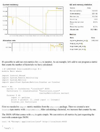
It's possible to add our own metrics for ekg to monitor. As an example, let's add to our program a metricthat counts the number of factorials we have calculated:

{-# LANGUAGE OverloadedStrings #-}module Main where

import Control.Monadimport System.Remote.Monitoringimport System.Metricsimport qualified System.Metrics.Counter as Counter

main = do server <- forkServer "localhost" 8000 factorials <- createCounter "factorials.count" (serverMetricStore server) forever $ do input <- getLine print $ product [1..read input :: Integer] Counter.inc factorials

First we needed to import metric modules from the ekg-core package. Then we created a newCountertype metric with createMetric. After calculating a factorial, we increase that counter by one.

The JSON API that comes with ekg is quite simple. We can retrieve all metrics by just requesting theroot with content-type JSON:

curl -H "Accept: application/json" http://localhost:8000

{ "ekg": {

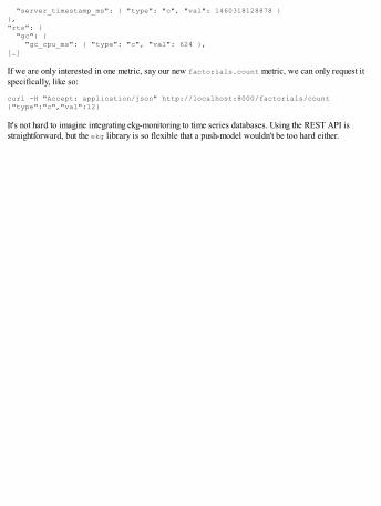
"server_timestamp_ms": { "type": "c", "val": 1460318128878 }},"rts": { "gc": { "gc_cpu_ms": { "type": "c", "val": 624 },[…]

If we are only interested in one metric, say our new factorials.count metric, we can only request itspecifically, like so:

curl -H "Accept: application/json" http://localhost:8000/factorials/count{"type":"c","val":12}

It's not hard to imagine integrating ekg-monitoring to time series databases. Using the REST API isstraightforward, but the ekg library is so flexible that a push-model wouldn't be too hard either.

SummaryWe started this chapter by profiling programs by cost centres, which can be set automatically (-fprof-auto) or manually (SCC-annotations). We learned that there is overhead in profiling, which is whyexecution times are an inaccurate metric when profiling. Allocations remained a good measure ofperformance in any case. We used the heap profiler to produce informative graphs about memory usageover time, and to spot unwanted allocations and retainers.

We explored different options in the GHC heap profiler: break-downs and subset selections, both ofwhich draw more or less from the same pool of parameters. The default break-down was by cost not yetfinished.

Finally, we looked at two additional libraries, criterion for benchmarking and ekg for monitoring. Indiscussing criterion, we stumbled upon the concept of normal form, which will also come up later onwhen we discuss parallelism. Adding real-time graphical garbage garbage collector monitoring viaHTTP to a Haskell application was a real breeze with ekg, and the library fully supports custom metricsand extending the monitoring system.

In the next chapter, we will pull everything together from these first three chapters and discuss some ofthe fine details of developing Haskell at scale: structuring bigger projects using cabal and stack. We willlook at some less common performance tricks such as lazy patterns and rewrite rules, revisit andintroduce some concepts such as inlining and specializing, and briefly discuss practical type-levelprogramming.

Chapter 4. The Devil's in the DetailIn this chapter, we pull together knowledge and techniques from previous chapters and learn to applythose techniques in large and complex projects. In particular, we will use cabal-install and stack tohelp us cope with multi-file projects and even projects with multiple subprojects. We learn how, andespecially how not, to throw and recover from exceptions in Haskell.

Having good test coverage is as important in a Haskell project as it is in projects written in any otherlanguage. But because Haskell's type-system is so expressive, the number of necessary test cases isgreatly reduced. Also, new extensions for the type-system in GHC are constantly being experimentedwith. Consequently, there is a bunch of language extensions considered more or less experimental, andsome extensions are just not enabled by default yet in the current standard (Haskell 2010).

This chapter concludes the first part of this book. Already from the three previous chapters, you are wellequipped to create and optimize programs in vanilla Haskell and to use some high-quality librarieseffectively. After this chapter, you will know how to structure Haskell projects of any size, handleexceptions correctly, and test code. In addition, we will look at the usual use cases for some newlanguage extensions. The following topics will be covered in this chapter:

Structuring larger projects using cabal-install and stackWriting tests for Haskell codeThrowing errors and handling exceptionsBest practices, tips, and tricks for writing robust, predictably fast HaskellGoing beyond Haskell 2010 with modern language features

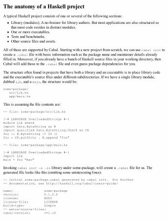
The anatomy of a Haskell projectA typical Haskell project consists of one or several of the following sections:

Library (modules); A no-brainer for library authors. But most applications are also structured sothat most code resides in distinct modules.One or more executables.Tests and benchmarks.Other source files and assets.

All of these are supported by Cabal. Starting with a new project from scratch, we can use cabal init tocreate a .cabal file with basic information such as the package name and maintainer details alreadyfilled in. Moreover, if you already have a bunch of Haskell source files in your working directory, thenCabal will add those to the .cabal file and even guess package dependencies for you.

The structure often found in projects that have both a library and an executable is to place library codeand the executable's source files under different subdirectories. If we have a single library module,dubbed Lib, and a main, the structure would be:

some-package/ src/Lib.hs app/main.hs

This is assuming the file contents are:

-- file: some-package/src/Lib.hs

{-# LANGUAGE OverloadedStrings #-}module Lib whereimport Data.ByteString as Bimport qualified Data.ByteString.Char8 as C8foo :: B.ByteString -> IO ()foo = C8.putStrLn . B.append "foo"

-- file: some-package/app/main.hs

{-# LANGUAGE OverloadedStrings #-}import Libmain = foo "bar"

Invoking cabal init -n –is library under some-package, will create a .cabal file for us. Thegenerated file looks like this (omitting some uninteresting lines):

-- Initial some-package.cabal generated by cabal init. For further-- documentation, see http://haskell.org/cabal/users-guide/

name: some-packageversion: 0.1.0.0license: BSD3license-file: LICENSEbuild-type: Simple-- extra-source-files: cabal-version: >=1.10

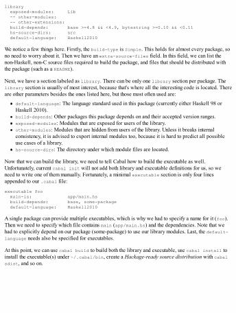
library exposed-modules: Lib -- other-modules: -- other-extensions: build-depends: base >=4.8 && <4.9, bytestring >=0.10 && <0.11 hs-source-dirs: src default-language: Haskell2010

We notice a few things here. Firstly, the build-type is Simple. This holds for almost every package, sono need to worry about it. Then we have an extra-source-files field. In this field, we can list thenon-Haskell, non-C source files required to build the package, and files that should be distributed withthe package (such as a README).

Next, we have a section labeled as library. There can be only one library section per package. Thelibrary section is usually of most interest, because that's where all the interesting code is located. Thereare other parameters besides the ones listed here, but those most often used are:

default-language: The language standard used in this package (currently either Haskell 98 orHaskell 2010).build-depends: Other packages this package depends on and their accepted version ranges.exposed-modules: Modules that are exposed for users of the library.other-modules: Modules that are hidden from users of the library. Unless it breaks internalconsistency, it is advised to export internal modules too, because it is hard to predict all possibleuse cases of a library.hs-source-dirs: The directory under which module files are located.

Now that we can build the library, we need to tell Cabal how to build the executable as well.Unfortunately, current cabal init will not add both library and executable definitions for us, so weneed to write one of them manually. Fortunately, a minimal executable section is only four linesappended to our .cabal file:

executable foo main-is: app/main.hs build-depends: base, some-package default-language: Haskell2010

A single package can provide multiple executables, which is why we had to specify a name for it (foo).Then we need to specify which file contains main (app/main.hs) and the dependencies. Note that wehad to explicitly depend on our package (some-package) to use our library modules. Last, the default-language needs also be specified for executables.

At this point, we can use cabal build to build both the library and executable, use cabal install toinstall the executable(s) under ~/.cabal/bin, create a Hackage-ready source distribution with cabalsdist, and so on.

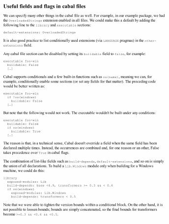
Useful fields and flags in cabal filesWe can specify many other things in the cabal file as well. For example, in our example package, we hadthe OverloadedStrings extension enabled in all files. We could make this a default by adding thefollowing line to the library and executable sections:

default-extensions: OverloadedStrings

It is also good practice to list conditionally used extensions (via LANGUAGE pragmas) in the other-extensions field.

Any cabal file section can be disabled by setting its buildable field to false, for example:

executable foo-win buildable: False […]

Cabal supports conditionals and a few built-in functions such as os(name), meaning we can, forexample, conditionally enable some sections (or set any fields for that matter). The preceding codewould be better written as:

executable foo-win if !os(windows) buildable: False […]

But note that the following would not work. The executable wouldn't be built under any conditions:

executable foo-win buildable: False if os(windows) buildable: True […]

The reason is that, in a technical sense, Cabal doesn't override a field when the same field has beendeclared multiple times. Instead, the occurrences are combined and, for one reason or an other, Falsetakes precedence over True in cabal flags.

The combination of list-like fields such as build-depends, default-extensions, and so on is simplythe union of all declarations. To build a Lib.Windows module only when building for a Windowsmachine, we could do this:

library exposed-modules: Lib build-depends: base <4.9, transformers >= 0.3 && < 0.6 if os(windows) exposed-modules: Lib.Windows build-depends: transformers < 0.5

Note that we were able to tighten the version bounds within a conditional block. On the other hand, it isnot possible to loosen bounds; bounds are simply concatenated, so the final bounds for transformersbecome >=0.3 && <0.6 && <0.5.

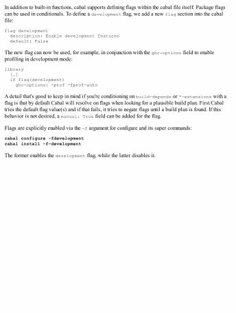
In addition to built-in functions, cabal supports defining flags within the cabal file itself. Package flagscan be used in conditionals. To define a development flag, we add a new flag section into the cabalfile:

flag development description: Enable development features default: False

The new flag can now be used, for example, in conjunction with the ghc-options field to enableprofiling in development mode:

library […] if flag(development) ghc-options: -prof -fprof-auto

A detail that's good to keep in mind if you're conditioning on build-depends or *-extensions with aflag is that by default Cabal will resolve on flags when looking for a plausible build plan. First Cabaltries the default flag value(s) and if that fails, it tries to negate flags until a build plan is found. If thisbehavior is not desired, a manual: True field can be added for the flag.

Flags are explicitly enabled via the -f argument for configure and its super commands:

cabal configure -fdevelopmentcabal install -f-development

The former enables the development flag, while the latter disables it.

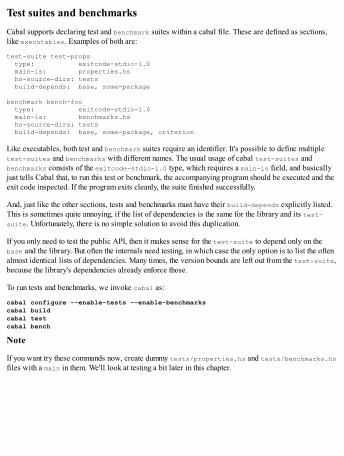
Test suites and benchmarksCabal supports declaring test and benchmark suites within a cabal file. These are defined as sections,like executables. Examples of both are:

test-suite test-props type: exitcode-stdio-1.0 main-is: properties.hs hs-source-dirs: tests build-depends: base, some-package

benchmark bench-foo type: exitcode-stdio-1.0 main-is: benchmarks.hs hs-source-dirs: tests build-depends: base, some-package, criterion

Like executables, both test and benchmark suites require an identifier. It's possible to define multipletest-suites and benchmarks with different names. The usual usage of cabal test-suites andbenchmarks consists of the exitcode-stdio-1.0 type, which requires a main-is field, and basicallyjust tells Cabal that, to run this test or benchmark, the accompanying program should be executed and theexit code inspected. If the program exits cleanly, the suite finished successfully.

And, just like the other sections, tests and benchmarks must have their build-depends explicitly listed.This is sometimes quite annoying, if the list of dependencies is the same for the library and its test-suite. Unfortunately, there is no simple solution to avoid this duplication.

If you only need to test the public API, then it makes sense for the test-suite to depend only on thebase and the library. But often the internals need testing, in which case the only option is to list the oftenalmost identical lists of dependencies. Many times, the version bounds are left out from the test-suite,because the library's dependencies already enforce those.

To run tests and benchmarks, we invoke cabal as:

cabal configure --enable-tests --enable-benchmarkscabal buildcabal testcabal bench

Note

If you want try these commands now, create dummy tests/properties.hs and tests/benchmarks.hsfiles with a main in them. We'll look at testing a bit later in this chapter.

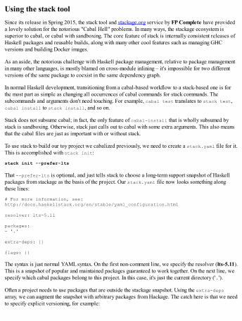
Using the stack toolSince its release in Spring 2015, the stack tool and stackage.org service by FP Complete have provideda lovely solution for the notorious "Cabal Hell" problems. In many ways, the stackage ecosystem issuperior to cabal, or cabal with sandboxing. The core feature of stack is internally consistent releases ofHaskell packages and reusable builds, along with many other cool features such as managing GHCversions and building Docker images.

As an aside, the notorious challenge with Haskell package management, relative to package managementin many other languages, is mostly blamed on cross-module inlining – it's impossible for two differentversions of the same package to coexist in the same dependency graph.

In normal Haskell development, transitioning from a cabal-based workflow to a stack-based one is forthe most part as simple as changing all occurrences of cabal commands for stack commands. Thesubcommands and arguments don't need touching. For example, cabal test translates to stack test,cabal install to stack install, and so on.

Stack does not subsume cabal; in fact, the only feature of cabal-install that is wholly subsumed bystack is sandboxing. Otherwise, stack just calls out to cabal with some extra arguments. This also meansthat the cabal files are just as important with or without stack.

To use stack to build our toy project we cabalized previously, we need to create a stack.yaml file for it.This is accomplished with stack init:

stack init --prefer-lts

That --prefer-lts is optional, and just tells stack to choose a long-term support snapshot of Haskellpackages from stackage as the basis of the project. Our stack.yaml file now looks something alongthese lines:

# For more information, see: http://docs.haskellstack.org/en/stable/yaml_configuration.html

resolver: lts-5.11

packages:- '.'

extra-deps: []

flags: {}

The syntax is just normal YAML syntax. On the first non-comment line, we specify the resolver (lts-5.11).This is a snapshot of popular and maintained packages guaranteed to work together. On the next line, wespecify which cabal packages belong to this project. In this case, it's just the current directory ('.').

Often a project needs to use packages that are outside the stackage snapshot. Using the extra-depsarray, we can augment the snapshot with arbitrary packages from Hackage. The catch here is that we needto specify explicit versioning, for example:

extra-deps:- acme-missiles-0.3

With the flags section, we tell stack to build packages with specific values of cabal flags. For example,we can enable the development flag in our project by default:

flags: some-package: development: true

For more configurables and stack commands, refer to the stack manual athttp://docs.haskellstack.org/en/stable/README.

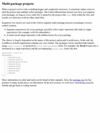
Multi-package projectsWhen a project evolves into something bigger and complexity increases, it sometimes makes sense tosplit the project into multiple cabal packages. The Cabal infrastructure doesn't care how you organizeyour packages, as long as every cabal file is named by the project (the name field within the file) andresides in a directory with no other cabal files.

In general, two tactics are seen in the wild to organize multi-package projects (assuming a versioncontrol system):

Separate repositories for every package, possibly with a super-repository that links to singlerepositories (for example with Git submodules)A catch-em-all mega-repository with subdirectories for every package

The choice is largely dependent on the nature of the project and people's preferences. In the end, theworkflows in both organization schemas are very similar. The packages can be installed individuallyusing cabal-install or declared in stack.yaml packages field. For example, the Yesod framework isstructured as a mega-repository and the accompanying stack.yaml looks like this:

resolver: lts-5.6packages: - ./yesod-core - ./yesod-static - ./yesod-persistent - ./yesod-form - ./yesod-auth - ./yesod-test - ./yesod-bin - ./yesod[…]

More information on cabal and stack can be found in their manuals. Also, the stackage.org site haspointers to many useful pieces of information. In the next section, we will leave structuring concernsbehind and get back to coding instead.

Erroring and handling exceptionsHaskell very intentionally does not have a null/None/nil value like many popular languages have, bothstrongly typed (Java) or not (Perl). Null values are exceptionally bad for program safety. Null values arenot expressed in types, giving nulls no choice but to hide from the unsuspecting programmer and pop intosight in production.

Nulls are one of the main causes of bugs and security holes in today's software, which is why Haskell hasopted for a no-null policy. This might sound restrictive at first, but actually the alternativerepresentations for possibly failing computations in Haskell are various and rich.

First, there are infinite ways to embed the possibility of failing into the datatype: Maybe, Either,YourAwesomeDataType, and so on.

Second, with the wonderfully extensive abstraction machinery in Haskell we can compose and recoverfrom failing situations on a very high level. Although these functors, monoids, monads, and whatnots havescarily abstract names "borrowed" from Category Theory, a branch of very abstract mathematics, theirincarnations in Haskell are easy to grasp and their benefits are many.

The worst way to handle any error in Haskell is to use error or undefined. Undefined particularly shouldalmost always be considered heresy – error is always better because at least an error message can begiven. Both error and undefined indicate an anomalous program state, from which recovery should not beattempted. Moreover, they are pure and asynchronous; a nightmare for referential transparency.

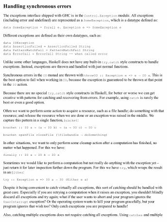
Handling synchronous errorsThe exceptions interface shipped with GHC is in the Control.Exception module. All exceptions(including error and undefined) are represented as a SomeException, which is a datatype defined as:

data SomeException = forall e. Exception e => SomeException e

Different exceptions are defined as their own datatypes, such as:

data IOExceptiondata AssertionFailed = AssertionFailed Stringdata PatternMatchFail = PatternMatchFail Stringdata ErrorCall = ErrorCall String -- when called error

Unlike some other languages, Haskell does not have any built-in try…catch style constructs to handleexceptions. Instead, exceptions are thrown and handled with just normal functions.

Synchronous errors in the IO monad are thrown with throwIO :: Exception e => e → IO a. This isthe best option to fail when working in IO, because the exception is guaranteed to be thrown at that pointin the IO action.

Because there are no special try…catch style constructs in Haskell, for better or worse we can getcreative with patterns for catching and recovering from errors. For example, using catch is rarely thebest or even a good option.

Often we want to perform some action to acquire a resource, such as a file handle; do something with thatresource; and release the resource when we are done or an exception was raised in the middle. Wecapture this pattern in a single function, bracket:

bracket :: IO a → (a → IO b) → (a → IO c) → IO c

bracket openFile closeFile (\fileHandle → doSomething)

In other situations, we want to only perform some cleanup action after a computation has finished, nomatter what happened. For this we have:

finally :: IO a → IO b → IO a

Sometimes we would like to perform a computation but not really do anything with the exception yet –just return it for later inspection further down the program. For this we have try, which wraps the resultin an Either:

try :: Exception e => IO a → IO (Either e a)

Despite it being convenient to catch virtually all exceptions, this sort of catching should be handled withgreat care. Especially if you are retrying a computation when it raises an exception, you shouldn't blindlydiscard all exceptions and try again; what if the user wants to abort and your program ignores theUserInterrupt exception? Or the operating system wants to kill your program gracefully, but yourprogram ignores that wish too? Only catch exceptions you are prepared to handle!

Also, catching multiple exceptions does not require catching all exceptions. Using catches and multiple

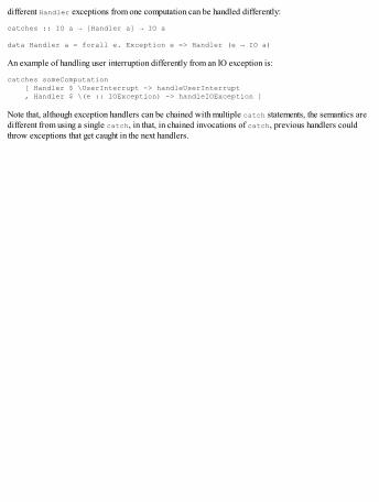
different Handler exceptions from one computation can be handled differently:

catches :: IO a → [Handler a] → IO a

data Handler a = forall e. Exception e => Handler (e → IO a)

An example of handling user interruption differently from an IO exception is:

catches someComputation [ Handler $ \UserInterrupt -> handleUserInterrupt , Handler $ \(e :: IOException) -> handleIOException ]

Note that, although exception handlers can be chained with multiple catch statements, the semantics aredifferent from using a single catch, in that, in chained invocations of catch, previous handlers couldthrow exceptions that get caught in the next handlers.

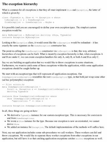
The exception hierarchyWhat is common for all exceptions is that they all must implement Show and Exception, the latter ofwhich is given by:

class (Typeable e, Show e) => Exception e where toException :: e → SomeException fromException :: SomeException → Maybe e

It is possible (and you are encouraged) to define your own exception types. The simplest customexception would be:

data MyException = MyException deriving (Show, Typeable)instance Exception MyException

Looking at the Exception class, it would seem like the toException would be redundant – it hasexactly the same signature as the SomeException constructor has.

The point in calling the SomeException constructor via toException is that, this way, arbitraryhierarchies of exceptions can be built. What is meant by exception hierarchy is that, when exceptions Aand B are under C, we can create exception handlers for only A, only B, or both A and B as only C.

Say we are building an application that we would like to throw exceptions in some situations.Furthermore, we want to catch some of those exceptions within the application, while some applicationexceptions should be caught further up.

We start with an exception type that will represent all application exceptions. OurSomeApplicationException resembles the root SomeException type, in that both just wrap some other(ad hoc polymorphic) exception:

-- file: errors.hsdata SomeApplicationException = forall e. Exception e => SomeApplicationException e deriving Typeable

instance Show SomeApplicationException where show (SomeApplicationException e) = "application: " ++ show e

instance Exception SomeApplicationException

In all, three things are going on here:

We derived a Typeable instance for our custom exception type. This is necessary for coercion toand from SomeExceptions.We wrote a Show instance for the type. Because our exception is now an existential, we cannotderive Show.We added an instance for Exception. The default implementations of the methods will suffice here.

Next, say our application includes some sub-procedures we call workers. These workers can fail andthrow exceptions. We would like to separate these worker exceptions from other exceptions in ourapplication, but still have it so that catching application exceptions catches worker exceptions as well.

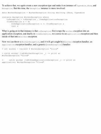
To achieve that, we again create a new exception type and make it an instance of Typeable, Show, andException. But this time, the Exception instance is more involved:

data WorkerException = WorkerException String deriving (Show, Typeable)

instance Exception WorkerException where toException = toException . SomeApplicationException fromException x = do SomeApplicationException e <- fromException x cast e

What is going on in that instance is that toException first wraps the worker exception into anapplication exception, and dually in fromException, we coerce to an application exception and theninside of that into a worker exception.

Now we can throw a WorkerException, and it will get caught by a worker exception handler, anapplication exception handler, and a generic (SomeException) handler:

> let worker = throwIO $ WorkerException "flood"

> catch worker (\e@(WorkerException _) -> print e)WorkerException "flood"

> catch worker (\e@(SomeApplicationException _) -> print e)application: WorkerException "flood"

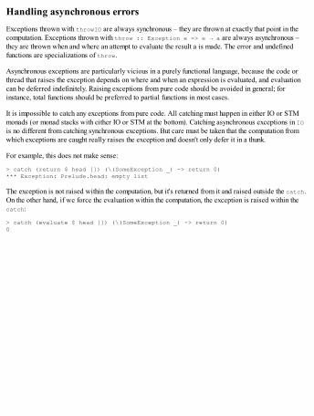
Handling asynchronous errorsExceptions thrown with throwIO are always synchronous – they are thrown at exactly that point in thecomputation. Exceptions thrown with throw :: Exception e => e → a are always asynchronous –they are thrown when and where an attempt to evaluate the result a is made. The error and undefinedfunctions are specializations of throw.

Asynchronous exceptions are particularly vicious in a purely functional language, because the code orthread that raises the exception depends on where and when an expression is evaluated, and evaluationcan be deferred indefinitely. Raising exceptions from pure code should be avoided in general; forinstance, total functions should be preferred to partial functions in most cases.

It is impossible to catch any exceptions from pure code. All catching must happen in either IO or STMmonads (or monad stacks with either IO or STM at the bottom). Catching asynchronous exceptions in IOis no different from catching synchronous exceptions. But care must be taken that the computation fromwhich exceptions are caught really raises the exception and doesn't only defer it in a thunk.

For example, this does not make sense:

> catch (return $ head []) (\(SomeException _) -> return 0)*** Exception: Prelude.head: empty list

The exception is not raised within the computation, but it's returned from it and raised outside the catch.On the other hand, if we force the evaluation within the computation, the exception is raised within thecatch:

> catch (evaluate $ head []) (\(SomeException _) -> return 0)0

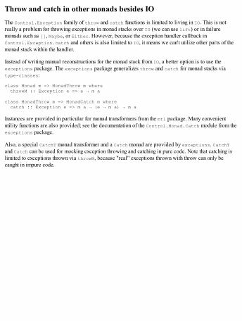
Throw and catch in other monads besides IOThe Control.Exception family of throw and catch functions is limited to living in IO. This is notreally a problem for throwing exceptions in monad stacks over IO (we can use lift) or in failuremonads such as [], Maybe, or Either. However, because the exception handler callback inControl.Exception.catch and others is also limited to IO, it means we can't utilize other parts of themonad stack within the handler.

Instead of writing manual reconstructions for the monad stack from IO, a better option is to use theexceptions package. The exceptions package generalizes throw and catch for monad stacks viatype-classes:

class Monad m => MonadThrow m where throwM :: Exception e => e → m a

class MonadThrow m => MonadCatch m where catch :: Exception e => m a → (e → m a) → m a

Instances are provided in particular for monad transformers from the mtl package. Many convenientutility functions are also provided; see the documentation of the Control.Monad.Catch module from theexceptions package.

Also, a special CatchT monad transformer and a Catch monad are provided by exceptions. CatchTand Catch can be used for mocking exception throwing and catching in pure code. Note that catching islimited to exceptions thrown via throwM, because "real" exceptions thrown with throw can only becaught in impure code.

Writing tests for HaskellThere are many libraries for testing Haskell code. Besides classic unit tests with HUnit and spec testingin Ruby-style with Hspec, we can verify properties using SmallCheck and QuickCheck with exhaustiveand randomized test cases, respectively.

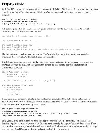
Property checksWith QuickCheck we can test properties in a randomized fashion. We don't need to generate the test casesourselves, as QuickCheck takes care of that. Here's a quick example of testing a simple arithmeticproperty:

stack ghci --package QuickCheck> import Test.QuickCheck as QC> QC.quickCheck $ \x y -> x > 0 ==> x + y >= y

All testable properties in QuickCheck are given as instances of the Testable class. As a quickreference, the core interface looks like this:

quickCheck :: Testable prop => prop → IO ()

class Testable prop where […]

instance Testable Propertyinstance Testable Boolinstance (Arbitrary a, Show a, Testable prop) => Testable (a → prop)

The last instance is perhaps most interesting. That's what allows us to test functions of variadicarguments directly with QuickCheck, like in our example.

QuickCheck generates test cases via the Arbitrary class. Instances for all the core types are given,provided they're sensible. Test case generators live in the Gen monad. Here is an example forclarification purposes:

class Arbitrary a where arbitrary :: Gen a shrink :: a → [a]

data D2 = D2 Double Double deriving (Eq, Show)

instance Arbitrary D2 where arbitrary = do x ← arbitrary y ← arbitrary return (x, y)

If you need more exhaustive checking than random test cases, then SmallCheck is a better choice.SmallCheck provides quantifiers, so we can express things such as "forall x exists y" and so forth. Hereis an example GHCi session using SmallCheck:

stack ghci --package smallcheck> import Test.SmallCheck as SC> smallCheck 2 $ forAll $ \x -> exists $ \y -> x + y > (x :: Int)Completed 22 tests without failure.

Like QuickCheck, SmallCheck supports testing properties as variadic functions. The smallCheckfunction requires an extra argument as its first argument, namely the depth of generated test cases. If thetest case has a reasonably bounded search space, such as Booleans, then it's possible to set the max depthto maxBound. SmallCheck then does an exhaustive check for the property.

For the simple cases, SmallCheck works a lot like QuickCheck. The default quantification context isforAll, which resembles that of QuickCheck. However, the test cases of QuickCheck are much betteroptimized for inexhustive testing, covering most usual corner cases, and QuickCheck automaticallyattempts to shrink the size of counter-examples.

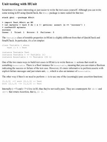
Unit testing with HUnitSometimes it is more interesting or just easier to write the test cases yourself. Although you can writesome testing in IO using QuickCheck, the HUnit package is more suited for that too:

stack ghci --package HUnit

> import Test.HUnit as HU> let mytests = test $ do { x <- getLine; assert (x == "success") }> runTestTT mytestssuccessCases: 1 Tried: 1 Errors: 0 Failures: 0

The Testable class of testable properties in HUnit is slightly different from that of QuickCheck andSmallCheck. In particular, it's a lot simpler:

class Testable t where test :: t → Test

instance Testable Testinstance Testable t => Testable [t]instance Assertable t => Testable (IO t)

One of the two main ways to build test cases in HUnit is to write them as IO actions that result insomething Assertable. There is a Bool instance for Assertable, meaning that you can return a Booleanindicating the success or failure of the test case. However, it's more informative to perform asserts withexplicit failure messages and just return unit, (), which is also an instance of Assertable.

The other way if there's no need to perform IO is to use one of the (seemingly) pure assertion functions:

[1,2,3] ~=? sort [2,1,3] :: Testsort [2,1,3] ~?= [1,2,3] :: Test

Internally (~=?) and (~?=) live in IO, thus they're not really pure. They are counterparts for (@=?) and(@?=) that return Assertion, that is, IO ().

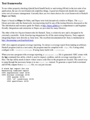
Test frameworksTo use either property checking (QuickCheck/SmallCheck) or unit testing (HUnit) in the test suite of anapplication, the use of a test framework simplifies things. A good test framework should also supportsome sort of resource management. Currently there are two main choices for a test framework in Haskell:Hspec and Tasty.

Hspec is based on RSpec for Ruby, and Hspec tests look deceptively similar to RSpec. The Hspeclibrary provides only the framework, leaving testing itself to any of the testing libraries discussed so far.The introduction and resource guide for Hspec at http://hspec.github.io is comprehensive and beginner-friendly. Integrations and extensions to Hspec are provided for many libraries.

The other of the two big test frameworks for Haskell, Tasty, is relatively new and is designed to beextremely extensible. Aside from having integrations for all the main testing libraries, Tasty supportsintegrating Hspec tests directly as Tasty tests. The excellent documentation for Tasty is maintained athttp://documentup.com/feuerbach/tasty.

GHC also supports program coverage reporting. To extract a coverage report from running an arbitraryHaskell program (such as a test suite), the program must be compiled with -fhpc. Or, if using cabal,configure with --enable-coverage. If using stack, build with --coverage.

When you run a program with coverage reporting, a <program>.tix file is generated. GHC comes withthe hpc command-line utility, which is used to inspect, combine, and do coverage reporting with .tixfiles. The hpc utility needs to know where source code files to the program are located. The easiest wayto jump through the necessary hoops is to use stack hpc instead. To generate a report both in terminaland HTML outputs from a foo.tix file, we can just execute:

$ stack hpc report foo.tixGenerating combined report100% expressions used (4/4)100% boolean coverage (0/0) 100% guards (0/0) 100% 'if' conditions (0/0) 100% qualifiers (0/0)

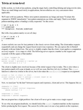
Trivia at term-levelIn this section, we look at lazy patterns, using the magic hash, controlling inlining and using rewrite rules.These are small things used rarely in applications, but nevertheless are very convenient whereapplicable.

We'll start with lazy patterns. Where strict pattern annotations use bangs and mean "Evaluate thisargument to WHNF immediately," lazy pattern annotations use tildes and imply "Don't even botherpattern-matching unless a binding is really requested." So this errors:

> let f (a,b) = 5> f undefined*** Exception: Prelude.undefined

But with a lazy pattern match, we are all okay:

> let f ~(a,b) = 5> f undefined5

A more realistic use case for lazy patterns is the classic server-client setting. The client makes requestssequentially and can change the request based on previous responses. We can express this in Haskellelegantly with just linked lists. The server is slightly simpler than the client: it just applies a computationon every request – it is a map or a fold. The following server expects a number as the request andresponds with the square of that number:

-- file: lazypat.hsserver :: [Int] -> [Int]server (y:ys) = process y : server ys where process n = n ^ 2

The client is slightly more involved, because of the initial request it has to make. This is also where alazy pattern match will come in handy, as we will see soon. But first, let's try it without. This clientfunction is otherwise similar to the server, but it also takes the next (initial) request as an argument:

client :: Int -> [Int] -> [Int]client initial (x:xs) = initial : client (next x) xs where next n = n `mod` 65534

Now, we need just "tie the knot" between requests and responses, client and server. This happens like so:

requests :: [Int]requests = client initial responses where initial = 2

responses :: [Int]responses = server requests

But our program has a slight problem. Our client will never get to make even a single request!

To see why our program deadlocks, we should look at the client: it pattern-matches on the responsesbefore producing the first request. The easiest fix in this case is to use a lazy pattern on the responses:

client :: Int -> [Int] -> [Int]client initial ~(x:xs) = initial : client (next x) xs where next n = n `mod` 65534

With that fix, we can now observe requests and responses as expected:

> :load lazypat.hs> take 10 responses[4,16,256,65536,4,16,256,65536,4,16]

With :sprint, we can inspect requests made and responses:

> :sprint responsesresponses = 4 : 16 : 256 : 65536 : 4 : 16 : 256 : 65536 : 4 : 16 : _> :sprint requestsrequests = 2 : 4 : 16 : 256 : 2 : 4 : 16 : 256 : 2 : 4 : _

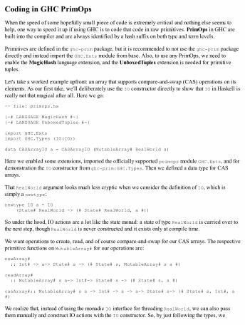
Coding in GHC PrimOpsWhen the speed of some hopefully small piece of code is extremely critical and nothing else seems tohelp, one way to speed it up if using GHC is to code that code in raw primitives. PrimOps in GHC arebuilt into the compiler and are always identified by a hash suffix on both type and term levels.

Primitives are defined in the ghc-prim package, but it is recommended to not use the ghc-prim packagedirectly and instead import the GHC.Exts module from base. Also, to use any PrimOps, we need toenable the MagicHash language extension, and the UnboxedTuples extension is needed for primitivetuples.

Let's take a worked example upfront: an array that supports compare-and-swap (CAS) operations on itselements. As our first take, we'll deliberately use the IO constructor directly to show that IO in Haskell isreally not that magical after all. Here we go:

-- file: primops.hs

{-# LANGUAGE MagicHash #-}{-# LANGUAGE UnboxedTuples #-}

import GHC.Extsimport GHC.Types (IO(IO))

data CASArrayIO a = CASArrayIO (MutableArray# RealWorld a)

Here we enabled some extensions, imported the officially supported primops module GHC.Exts, and fordemonstration the IO constructor from ghc-prim:GHC.Types. Then we defined a data type for CASarrays.

That RealWorld argument looks much less cryptic when we consider the definition of IO, which issimply a newtype:

newtype IO a = IO (State# RealWorld -> (# State# RealWorld, a #))

So under the hood, IO actions are a lot like the state monad: a state of type RealWorld is carried over tothe next step, though RealWorld is never constructed and it exists only at compile time.

We want operations to create, read, and of course compare-and-swap for our CAS arrays. The respectiveprimitive functions on MutableArray# for our operations are:

newArray# :: Int# -> a-> State# s -> (# State# s, MutableArray# s a #)

readArray# :: MutableArray# s a-> Int#-> State# s -> (# State# s, a #)

casArray#:: MutableArray# s a -> Int# -> a -> a-> State# s-> (# State# s, Int#, a #)

We realize that, instead of using the monadic IO interface for threading RealWorld, we can also passthem manually and construct IO actions with the IO constructor. So, by just following the types, we

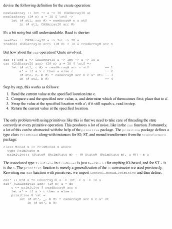
devise the following definition for the create operation:

newCasArray :: Int -> a -> IO (CASArrayIO a)newCasArray (I# n) a = IO $ \st0 -> let (# st1, arr #) = newArray# n a st0 in (# st1, CASArrayIO arr #)

It's a bit noisy but still understandable. Read is shorter:

readCas :: CASArrayIO a -> Int -> IO areadCas (CASArrayIO arr) (I# n) = IO $ readArray# arr n

But how about the cas operation? Quite involved:

cas :: Ord a => CASArrayIO a -> Int -> a -> IO acas (CASArrayIO arr) (I# n) a = IO $ \st0 -> let (# st1, c #) = readArray# arr n st0 -- 1 a' = if a > c then a else c –- 2 (# st2, r, b #) = casArray# arr n c a' st1 -- 3 in (# st2, b #) -- 4

Step by step, this works as follows:

1. Read the current value at the specified location into c.2. Compare c and the specified new value, a, and determine which of them comes first; place that to a'.3. Swap the value at the specified location with a'; if it still equals c, read in step.4. Return the current value at the specified location.

The only problem with using primitives like this is that we need to take care of threading the statecorrectly at every primitive operation. This produces a lot of noise, like in the cas function. Fortunately,a lot of this can be abstracted with the help of the primitive package. The primitive package defines atype class PrimMonad along with instances for IO, ST, and monad transformers from the transformerspackage:

class Monad m => PrimMonad m where type PrimState m primitive:: (State# (PrimState m) → (# State# (PrimState m), a #))→ m a

The associated type PrimState in PrimMonad is just RealWorld for anything IO-based, and for ST s itis the s. The primitive function is merely a generalization of the IO constructor we used previously.Rewriting our cas function with primitives, we import Control.Monad.Primitive and then define:

cas' :: Ord a => CASArrayIO a -> Int -> a -> IO acas' (CASArrayIO arr) (I# n) a = do c <- primitive $ readArray# arr n let a' = if a > c then a else c primitive $ \st → let (# st', _, b #) = casArray# arr n c a' st in (# st', b #)

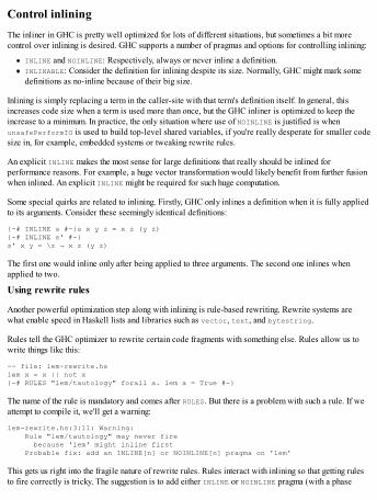
Control inliningThe inliner in GHC is pretty well optimized for lots of different situations, but sometimes a bit morecontrol over inlining is desired. GHC supports a number of pragmas and options for controlling inlining:

INLINE and NOINLINE: Respectively, always or never inline a definition.INLINABLE: Consider the definition for inlining despite its size. Normally, GHC might mark somedefinitions as no-inline because of their big size.

Inlining is simply replacing a term in the caller-site with that term's definition itself. In general, thisincreases code size when a term is used more than once, but the GHC inliner is optimized to keep theincrease to a minimum. In practice, the only situation where use of NOINLINE is justified is whenunsafePerformIO is used to build top-level shared variables, if you're really desperate for smaller codesize in, for example, embedded systems or tweaking rewrite rules.

An explicit INLINE makes the most sense for large definitions that really should be inlined forperformance reasons. For example, a huge vector transformation would likely benefit from further fusionwhen inlined. An explicit INLINE might be required for such huge computation.

Some special quirks are related to inlining. Firstly, GHC only inlines a definition when it is fully appliedto its arguments. Consider these seemingly identical definitions:

{-# INLINE s #-}s x y z = x z (y z){-# INLINE s' #-}s' x y = \z → x z (y z)

The first one would inline only after being applied to three arguments. The second one inlines whenapplied to two.

Using rewrite rules

Another powerful optimization step along with inlining is rule-based rewriting. Rewrite systems arewhat enable speed in Haskell lists and libraries such as vector, text, and bytestring.

Rules tell the GHC optimizer to rewrite certain code fragments with something else. Rules allow us towrite things like this:

-- file: lem-rewrite.hslem x = x || not x{-# RULES "lem/tautology" forall a. lem a = True #-}

The name of the rule is mandatory and comes after RULES. But there is a problem with such a rule. If weattempt to compile it, we'll get a warning:

lem-rewrite.hs:3:11: Warning: Rule "lem/tautology" may never fire because 'lem' might inline first Probable fix: add an INLINE[n] or NOINLINE[n] pragma on 'lem'

This gets us right into the fragile nature of rewrite rules. Rules interact with inlining so that getting rulesto fire correctly is tricky. The suggestion is to add either INLINE or NOINLINE pragma (with a phase

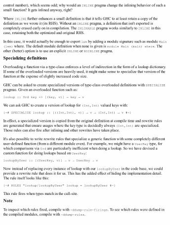
control number), which seems odd; why would an INLINE pragma change the inlining behavior of such asmall function? It gets inlined anyway, right?

Where INLINE further enhances a small definition is that it tells GHC to at least retain a copy of thedefinition as we wrote it (its RHS). Without an INLINE pragma, a definition that isn't exported iscompletely erased early on in compilation. The INLINABLE pragma works similarly to INLINE in thiscase, retaining both the optimized and original RHS.

In this case, it would actually be enough to export lem by adding a module signature such as module Main(lem) where. The default module definition when none is given is module Main (main) where. Theother (better) option is to use an explicit INLINE or NOINLINE pragma.

Specializing definitions

Overloading a function via a type-class enforces a level of indirection in the form of a lookup dictionary.If some of the overloaded versions are heavily used, it might make sense to specialize that version of thefunction at the expense of slightly increased code size.

GHC can be asked to create specialized versions of type-class overloaded definitions with SPECIALIZEpragmas. Given an overloaded function such as:

lookup :: Ord key => [(key, v)] → key → v

We can ask GHC to create a version of lookup for (Int,Int) valued keys with:

{-# SPECIALIZE lookup :: [((Int,Int), v)] → v → (Int,Int) → v #-}

In effect, a specialized version is copied from the original definition at compile time and rewrite rulesare generated that ensure usages where the key type is decidedly always (Int,Int) are specialized.Those rules can also fire after inlining and other rewrites have taken place.

It's also possible to write rewrite rules that specialize a generic function with some completely differentuser-defined function (from a different module even). For example, we might have a UserKey type, forwhich comparisons via Ord are particularly inefficient when doing a lookup. So we have devised acustom function for doing lookups based on UserKey:

lookupByUser :: [(UserKey, v)] → v → UserKey → v

Now instead of replacing every instance of lookup with our lookupByUser in the code base, we couldprovide a rewrite rule that does it for us. This has the added effect of hiding the implementation detail.The rule itself looks like this:

{-# RULES "lookup/lookupByUser" lookup = lookupByUser #-}

This rule fires when types match in the call-site.

Note

To inspect which rules fired, compile with -ddump-rule-firings. To see which rules were defined inthe compiled modules, compile with -ddump-rules.

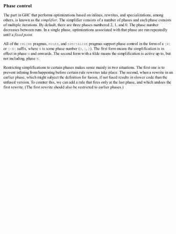
Phase control

The part in GHC that performs optimizations based on inlines, rewrites, and specializations, amongothers, is known as the simplifier. The simplifier consists of a number of phases and each phase consistsof multiple iterations. By default, there are three phases numbered 2, 1, and 0. The phase numberdecreases between runs. In a single phase, optimizations associated with that phase are run repeatedlyuntil a fixed point.

All of the INLINE pragmas, RULES, and SPECIALIZE pragmas support phase control in the form of a [N]or [~N] suffix, where N is some phase number (0, 1, 2). The first form means the simplification is ineffect in phase N and onwards. The second form with a tilde means the simplification is active up to, butnot including, phase N.

Restricting simplifications to certain phases makes sense mainly in two situations. The first one is toprevent inlining from happening before certain rule rewrites take place. The second, when a rewrite in anearlier phase, which might subject the definition for fusion, if not fused results in slower code than theunfused version. To counter this, we can add a rule that fires only at the last phase, and which undoes thefirst rewrite. (The first rewrite should also be restricted to earlier phases.)

Trivia at type-levelThe more expressive the types are, the more safety we can ensure at compile-time. What's more,expressive types serve as documentation that is always up-to-date.

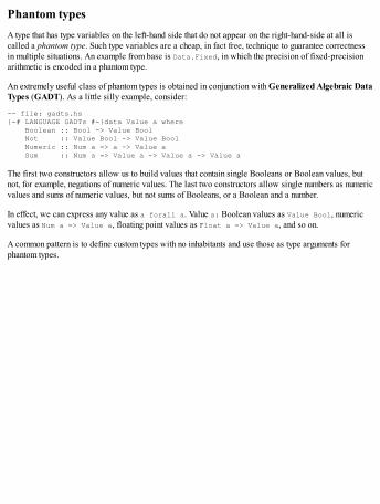
Phantom typesA type that has type variables on the left-hand side that do not appear on the right-hand-side at all iscalled a phantom type. Such type variables are a cheap, in fact free, technique to guarantee correctnessin multiple situations. An example from base is Data.Fixed, in which the precision of fixed-precisionarithmetic is encoded in a phantom type.

An extremely useful class of phantom types is obtained in conjunction with Generalized Algebraic DataTypes (GADT). As a little silly example, consider:

-- file: gadts.hs{-# LANGUAGE GADTs #-}data Value a where Boolean :: Bool -> Value Bool Not :: Value Bool -> Value Bool Numeric :: Num a => a -> Value a Sum :: Num a => Value a -> Value a -> Value a

The first two constructors allow us to build values that contain single Booleans or Boolean values, butnot, for example, negations of numeric values. The last two constructors allow single numbers as numericvalues and sums of numeric values, but not sums of Booleans, or a Boolean and a number.

In effect, we can express any value as a forall a. Value a: Boolean values as Value Bool, numericvalues as Num a => Value a, floating point values as Float a => Value a, and so on.

A common pattern is to define custom types with no inhabitants and use those as type arguments forphantom types.

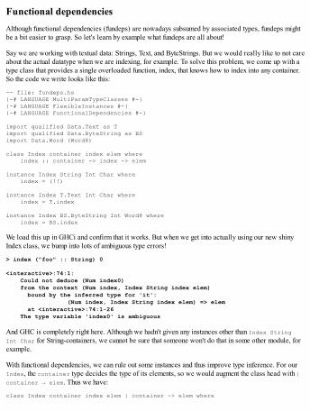
Functional dependenciesAlthough functional dependencies (fundeps) are nowadays subsumed by associated types, fundeps mightbe a bit easier to grasp. So let's learn by example what fundeps are all about!

Say we are working with textual data: Strings, Text, and ByteStrings. But we would really like to not careabout the actual datatype when we are indexing, for example. To solve this problem, we come up with atype class that provides a single overloaded function, index, that knows how to index into any container.So the code we write looks like this:

-- file: fundeps.hs{-# LANGUAGE MultiParamTypeClasses #-}{-# LANGUAGE FlexibleInstances #-}{-# LANGUAGE FunctionalDependencies #-}

import qualified Data.Text as Timport qualified Data.ByteString as BSimport Data.Word (Word8)

class Index container index elem where index :: container -> index -> elem

instance Index String Int Char where index = (!!)

instance Index T.Text Int Char where index = T.index

instance Index BS.ByteString Int Word8 where index = BS.index

We load this up in GHCi and confirm that it works. But when we get into actually using our new shinyIndex class, we bump into lots of ambiguous type errors!

> index ("foo" :: String) 0

<interactive>:74:1: Could not deduce (Num index0) from the context (Num index, Index String index elem) bound by the inferred type for 'it': (Num index, Index String index elem) => elem at <interactive>:74:1-26 The type variable 'index0' is ambiguous

And GHC is completely right here. Although we hadn't given any instances other than Index StringInt Char for String-containers, we cannot be sure that someone won't do that in some other module, forexample.

With functional dependencies, we can rule out some instances and thus improve type inference. For ourIndex, the container type decides the type of its elements, so we would augment the class head with |container → elem. Thus we have:

class Index container index elem | container -> elem where

index :: container -> index -> elem

We could also, if desired, have written container → elem index to say that the container decidesboth element and index types, or container index → elem for container and index together decidingthe type of element. The latter would be useful to allow instances such as Index String (Int, Int)String, that is, using a range as the index to return a substring.

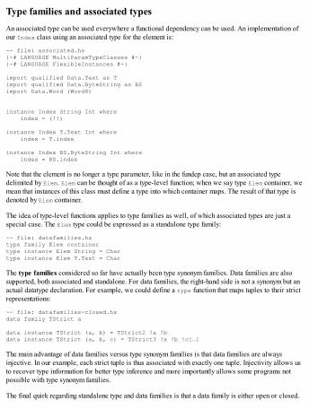
Type families and associated typesAn associated type can be used everywhere a functional dependency can be used. An implementation ofour Index class using an associated type for the element is:

-- file: associated.hs{-# LANGUAGE MultiParamTypeClasses #-}{-# LANGUAGE FlexibleInstances #-}

import qualified Data.Text as Timport qualified Data.ByteString as BSimport Data.Word (Word8)

instance Index String Int where index = (!!)

instance Index T.Text Int where index = T.index

instance Index BS.ByteString Int where index = BS.index

Note that the element is no longer a type parameter, like in the fundep case, but an associated typedelimited by Elem. Elem can be thought of as a type-level function; when we say type Elem container, wemean that instances of this class must define a type into which container maps. The result of that type isdenoted by Elem container.

The idea of type-level functions applies to type families as well, of which associated types are just aspecial case. The Elem type could be expressed as a standalone type family:

-- file: datafamilies.hstype family Elem containertype instance Elem String = Chartype instance Elem T.Text = Char

The type families considered so far have actually been type synonym families. Data families are alsosupported, both associated and standalone. For data families, the right-hand side is not a synonym but anactual datatype declaration. For example, we could define a type function that maps tuples to their strictrepresentations:

-- file: datafamilies-closed.hsdata family TStrict a

data instance TStrict (a, b) = TStrict2 !a !bdata instance TStrict (a, b, c) = TStrict3 !a !b !c[…]

The main advantage of data families versus type synonym families is that data families are alwaysinjective. In our example, each strict tuple is thus associated with exactly one tuple. Injectivity allows usto recover type information for better type inference and more importantly allows some programs notpossible with type synonym families.

The final quirk regarding standalone type and data families is that a data family is either open or closed.

In an open type family, new instances can be defined wherever the family is in scope, and also indifferent modules. But all instances of a closed type family must be specified in a where clause right afterdeclaring the family. Strict tuples as a closed type family would look like this:

data family TStrict a where TStrict (a, b) = TStrict2 !a !b TStrict (a, b, c) = TStrict3 !a !b !c […]

Useful GHC extensionsWe have already used a number of extensions available in GHC, such as MultiParamTypeClasses,TypeFamilies, FlexibleInstances, and so on. The nice thing about most extensions in GHC is that, if youaccidentally try to use a language feature that is behind an extension, GHC gives you a hint about whichextension you forgot.

In this last section, we'll look at some more useful extensions available in reasonably modern GHC.There are other extensions, of course, and this is just a glimpse. For an exhaustive list of currentlysupported extensions, see the Language.Haskell.Extension module from the Cabal library.

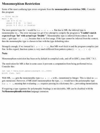
Monomorphism RestrictionSome of the most confusing type errors originate from the monomorphism restriction (MR). Considerthis program:

-- file: mr.hsmain = do let f = (1 +) print $ f (6 :: Int) print $ f (0.1 :: Double)

The most general type for f would be Num a => a → a. But due to MR, the inferred type ismonomorphic in a. The error message we get if we attempt to compile the program is "Couldn't matchexpected type 'Int' with actual type 'Double'". Monomorphic type is inferred from context. In ourcase, f gets type Int → Int, because that is its first usage. If the type cannot be inferred from the context,then the monomorphic type is chosen in line with the type defaulting rules.

Strangely enough, if we instead let f x = (1 + x), then MR won't kick in and the program compiles justfine. In this regard, function syntax is very much different from pattern syntax (f = \x → 1 + x).

Note

Monomorphism restriction has been on by default in compiled code, and off in GHCi, since GHC 7.8.1.

The motivation for MR is that in some cases it prevents a computation from being performed twice.Consider this:

let len = Data.List.genericLength [1..1000]print (len, len)

With MR, len gets the monomorphic type Num a => a with a instantiated to Integer. This is ideal as lengets memoized. However, if MR didn't monomorphize the type, len would have the polymorphic typeNum a => a, meaning that evaluating len requires passing in a dictionary for a, preventing memoization.

If requiring a type signature for polymorphic bindings is not desirable, MR can be disabled with theNoMonomorphismRestriction language extension.

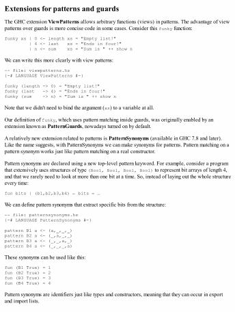
Extensions for patterns and guardsThe GHC extension ViewPatterns allows arbitrary functions (views) in patterns. The advantage of viewpatterns over guards is more concise code in some cases. Consider this funky function:

funky xs | 0 <- length xs = "Empty list!" | 4 <- last xs = "Ends in four!" | n <- sum xs = "Sum is " ++ show n

We can write this more clearly with view patterns:

-- file: viewpatterns.hs{-# LANGUAGE ViewPatterns #-}

funky (length -> 0) = "Empty list!"funky (last -> 4) = "Ends in four!"funky (sum -> n) = "Sum is " ++ show n

Note that we didn't need to bind the argument (xs) to a variable at all.

Our definition of funky, which uses pattern matching inside guards, was originally enabled by anextension known as PatternGuards, nowadays turned on by default.

A relatively new extension related to patterns is PatternSynonyms (available in GHC 7.8 and later).Like the name suggests, with PatternSynonyms we can make synonyms for patterns. Pattern matching on apattern synonym works just like pattern matching on a real constructor.

Pattern synonyms are declared using a new top-level pattern keyword. For example, consider a programthat extensively uses structures of type (Bool, Bool, Bool, Bool) to represent bit arrays of length 4,and that we rarely need to look at more than one bit at a time. So, instead of laying out the whole structureevery time:

fun bits | (b1,b2,b3,b4) ← bits = …

We can define pattern synonyms that extract specific bits from the structure:

-- file: patternsynonyms.hs{-# LANGUAGE PatternSynonyms #-}

pattern B1 a <- (a,_,_,_)pattern B2 a <- (_,a,_,_)pattern B3 a <- (_,_,a,_)pattern B4 a <- (_,_,_,a)

These synonyms can be used like this:

fun (B1 True) = 1fun (B2 True) = 2fun (B3 True) = 3fun (B4 True) = 4

Pattern synonyms are identifiers just like types and constructors, meaning that they can occur in exportand import lists.

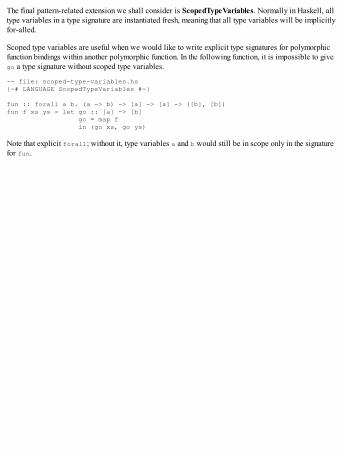
The final pattern-related extension we shall consider is ScopedTypeVariables. Normally in Haskell, alltype variables in a type signature are instantiated fresh, meaning that all type variables will be implicitlyfor-alled.

Scoped type variables are useful when we would like to write explicit type signatures for polymorphicfunction bindings within another polymorphic function. In the following function, it is impossible to givego a type signature without scoped type variables.

-- file: scoped-type-variables.hs{-# LANGUAGE ScopedTypeVariables #-}

fun :: forall a b. (a -> b) -> [a] -> [a] -> ([b], [b])fun f xs ys = let go :: [a] -> [b] go = map f in (go xs, go ys)

Note that explicit forall; without it, type variables a and b would still be in scope only in the signaturefor fun.

Strict-by-default HaskellTwo of the new features added in GHC 8.0.1 are the Strict and StrictData extensions, that changeHaskell from a lazy-by-default language into a strict-by-default language (on a per-module basis).

When StrictData is in effect, fields in the data declaration are considered as if they had a strictnessannotation (!) in front, unless the field is explicitly set to lazy with the laziness annotation (~):

data S = S a -- 1data S = S !a -- 2data S = S ~a -- 3

Under normal circumstances, (1) is interpreted as (3), but under StrictData it is interpreted as (2).Writing laziness annotations is not allowed unless StrictData is enabled.

On the other hand, the Strict extension adds a bang to all pattern bindings everywhere in the module. WithStrict in effect, normal irrefutable patterns, ~(x,y), become just lazy patterns. Irrefutable patterns can berecovered with ~(~(x,y)).

SummaryWe began this chapter by looking at what Haskell projects usually consist of and how Cabal and stack areused to manage project complexity and dependencies. We glanced at the basic usage of main test librariesand frameworks for Haskell and how they can be integrated into a cabalized project. We learned how tohandle errors and exceptions. Even more importantly, we learned how to not do errors; why preferthrowIO over error (or throw)? Why are asynchronous errors so vicious in lazy semantics?

In the latter part of this chapter, we explored some Haskell trivia and techniques specific to GHC: lazypatterns, coding with GHC primitives (the magic hash), inlining, writing rewrite rules, using phantomtypes, fundeps, type families, the monomorphism restriction, and some useful GHC extensions. Now youshould be able to both read and write cabal files, devise test suites with test libraries (QuickCheck,SmallCheck, and HUnit) and test frameworks (Hspec, Tasty), and throw and catch exceptions correctly;you should also have absorbed some trivia about Haskell and GHC.

In the next chapter, we will look at parallelization and RePa, a Haskell library for high-performanceparallel array programming.

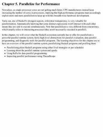
Chapter 5. Parallelize for PerformanceNowadays, as single processor cores are not getting much faster, CPU manufacturers instead keepincreasing the number of cores in processors, implying that high-performance programs must accordinglyexploit more and more parallelism to keep up with this breadth-wise hardware development.

Turns out, one of Haskell's strongest aspects, referential transparency, is very valuable forparallelization. Automatically knowing that some distinct expressions won't interact with each othermeans they are safe to execute simultaneously. Note that parallelism is very different from concurrency,which usually refers to interacting processes (they aren't necessarily executed in parallel).

In this chapter, we will cover what the Haskell ecosystem currently has to offer for parallelism: apowerful parallel runtime system, fairly high-level abstractions for parallel evaluation, data parallelprogramming, and diagnostic tools for parallel programs. The learning objectives for this chapter are tohave an overview of the parallel runtime system, parallelizing Haskell programs and profiling them:

Parallelizing plain Haskell programs using either Eval strategies or par schedulesLearning about the parallel runtime system and sparksUsing RePa for data parallel programmingInspecting parallel performance using ThreadScope

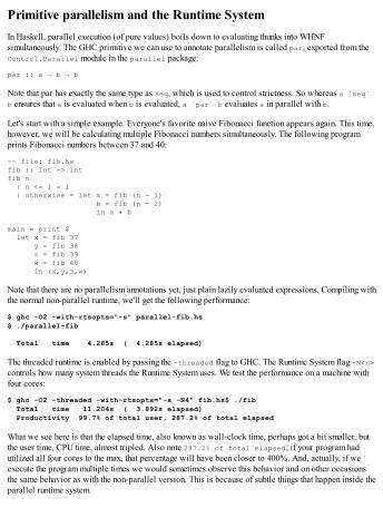
Primitive parallelism and the Runtime SystemIn Haskell, parallel execution (of pure values) boils down to evaluating thunks into WHNFsimultaneously. The GHC primitive we can use to annotate parallelism is called par, exported from theControl.Parallel module in the parallel package:

par :: a → b → b

Note that par has exactly the same type as seq, which is used to control strictness. So whereas a `seq`b ensures that a is evaluated when b is evaluated, a `par` b evaluates a in parallel with b.

Let's start with a simple example. Everyone's favorite naive Fibonacci function appears again. This time,however, we will be calculating multiple Fibonacci numbers simultaneously. The following programprints Fibonacci numbers between 37 and 40:

-- file: fib.hsfib :: Int -> Intfib n | n <= 1 = 1 | otherwise = let a = fib (n - 1) b = fib (n - 2) in a + b

main = print $ let x = fib 37 y = fib 38 z = fib 39 w = fib 40 in (x,y,z,w)

Note that there are no parallelism annotations yet, just plain lazily evaluated expressions. Compiling withthe normal non-parallel runtime, we'll get the following performance:

$ ghc -O2 -with-rtsopts="-s" parallel-fib.hs$ ./parallel-fib

Total time 4.285s ( 4.285s elapsed)

The threaded runtime is enabled by passing the -threaded flag to GHC. The Runtime System flag -N<n>controls how many system threads the Runtime System uses. We test the performance on a machine withfour cores:

$ ghc -O2 -threaded -with-rtsopts="-s -N4" fib.hs$ ./fib Total time 11.204s ( 3.892s elapsed) Productivity 99.7% of total user, 287.2% of total elapsed

What we see here is that the elapsed time, also known as wall-clock time, perhaps got a bit smaller, butthe user time, CPU time, almost tripled. Also note 287.2% of total elapsed; if your program hadutilized all four cores to the max, that percentage will have been closer to 400%. And, actually, if weexecute the program multiple times we would sometimes observe this behavior and on other occasionsthe same behavior as with the non-parallel version. This is because of subtle things that happen inside theparallel runtime system.

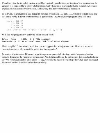
It's unlikely that the threaded runtime would have actually parallelized our thunks of fib expressions. Ingeneral, it is impossible to know whether it is actually beneficial to evaluate thunks in parallel, becauseexpressions can share subexpressions, and moving data between threads is expensive.

To tell GHC to evaluate our fib thunks in parallel, we can use par and pseq, which is semantically likeseq but is subtly different when it comes to parallelism. The parallelized program looks like this:

let x = fib 37 y = fib 38 z = fib 39 w = fib 40 in x `par` y `par` z `par` w `pseq` (x, y, z, w)

With this our program now performs better on four cores:

Total time 6.698s ( 1.739s elapsed)Productivity 99.9% of total user, 384.7% of total elapsed

That's roughly 2.5 times faster with four cores as opposed to with just one core. However, we wererunning four cores; why wasn't the speed four times greater?

Remember that the naive Fibonacci algorithm grows exponentially in time, so the largest evaluationactually dominates the runtime of our program. We didn't parallelize the calculation itself, and calculatingthe 40th Fibonacci number takes about 1.7 sec, which is the best we could hope for when each individualFibonacci number is still calculated sequentially.

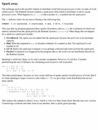
Spark awayThe technique used in the parallel runtime to distribute work between processors works via units of workcalled sparks. The Runtime System contains a spark pool, from which it distributes work to vacantprocessor cores. What happens in par x y is that a pointer to x is pushed into the spark pool.

The -s statistics show for our naive Fibonacci the following line:

SPARKS: 3 (3 converted, 0 overflowed, 0 dud, 0 GC'd, 0 fizzled)

This says that our program generated three sparks (from three calls to par), the evaluation of which wasentirely initiated from the spark pool by the Runtime System (converted). Other things that can happenfor a spark in a spark pool include:

Overflowed: The spark was not added into the spark pool, because the pool was at its maximumcapacity.Dud: When the argument to par is already evaluated, it's counted as dud. The spark pool is nottouched at all.GC'd: Before the spark got evaluated, it was garbage-collected and removed from the spark pool.Fizzled: Evaluation was triggered by the program; that is, the work was not distributed directly bythe Runtime System.

Sparking is relatively cheap, as it's only a pointer assignment. However, it's not free. Considerparallelizing the naive Fibonacci by calculating each recursive call in parallel:

let a = fib (n - 1) b = fib (n - 2) in a `par` b `par` a + b

This hurts performance, because we now create millions of sparks mostly of small pieces of work. But ifwe limit sparking to larger recursive calls where n > 25, we get a finer work distribution but not toomany sparks:

fib n | n <= 1 = 1 | n <= 25 = fib (n - 1) + fib (n - 2) | otherwise = let a = fib (n - 1) b = fib (n - 2) in a `par` b `par` a + b

This reduces the runtime to about 1.4 sec, which is a bit over three times faster than the one-core version.Considering overheads and other load on my machine, that's a pretty good speedup.

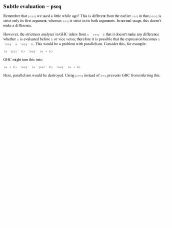
Subtle evaluation – pseqRemember that pseq we used a little while ago? This is different from the earlier seq in that pseq isstrict only its first argument, whereas seq is strict in its both arguments. In normal usage, this doesn'tmake a difference.

However, the strictness analyzer in GHC infers from a `seq` b that it doesn't make any differencewhether a is evaluated before b or vice versa; therefore it is possible that the expression becomes b`seq` a `seq` b. This would be a problem with parallelism. Consider this, for example:

(a `par` b) `seq` (a + b)

GHC might turn this into:

(a + b) `seq` (a `par` b) `seq` (a + b)

Here, parallelism would be destroyed. Using pseq instead of seq prevents GHC from inferring this.

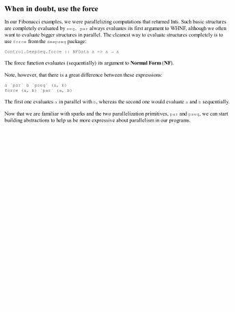
When in doubt, use the forceIn our Fibonacci examples, we were parallelizing computations that returned Ints. Such basic structuresare completely evaluated by seq. par always evaluates its first argument to WHNF, although we oftenwant to evaluate bigger structures in parallel. The cleanest way to evaluate structures completely is touse force from the deepseq package:

Control.DeepSeq.force :: NFData a => a → a

The force function evaluates (sequentially) its argument to Normal Form (NF).

Note, however, that there is a great difference between these expressions:

a `par` b `pseq` (a, b)force (a, b) `par` (a, b)

The first one evaluates a in parallel with b, whereas the second one would evaluate a and b sequentially.

Now that we are familiar with sparks and the two parallelization primitives, par and pseq, we can startbuilding abstractions to help us be more expressive about parallelism in our programs.

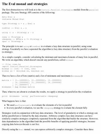
The Eval monad and strategiesThe first abstraction we will look at is the Control.Parallel.Strategies module from the parallelpackage. The core Strategy API consists of the following:

data Eval ainstance Monad Eval

type Strategy a = a → Eval a

runEval :: Eval a → a

using :: a → Strategy a → a

rseq :: Strategy ardeepseq :: NFData a => Strategy arpar :: Strategy a

The principle is to use using or runEval to evaluate a lazy data structure in parallel, using somestrategy. Essentially we have separated the algorithm (a lazy data structure) from the parallel evaluation(a strategy).

As a simple example, consider calculating the minimum and maximum elements of many lists in parallel.We write an algorithm, which doesn't encode any parallelism, called minmax:

-- file: rows.hsimport Control.Parallel.Strategiesminmax :: [Int] -> (Int, Int)minmax xs = (minimum xs, maximum xs)

Then we have a list of lists (matrix) and a list of minimums and maximums (minmaxes):

matrix = [ [1..1000001], [2..2000002], [3..2000003] , [4..2000004], [5..2000005], [6..2000006] , [7..2000007] ]minmaxes = map minmax matrix

Then, when we are about to evaluate the results, we apply a strategy to parallelize the evaluation:

print (minmaxes `using` parTraversable rdeepseq)

What happens here is that:

We used parTraversable to evaluate the elements of a list in parallelIn every parallel evaluation, we use the rdeepseq strategy to evaluate the element fully

Strategies work in conjunction with lazy data structures. The level of granularity at which a strategy candefine parallelism is limited by the data structure. Arbitrary complex lazy data structures can havesimilarly complex strategies completely separated from the algorithm that builds the structure. However,data dependencies in the algorithm limit the possible benefits of applying parallel strategies, becausecopying data between threads is not free.

Directly using the Eval monad, we can express arbitrarily complex strategies. Consider these three

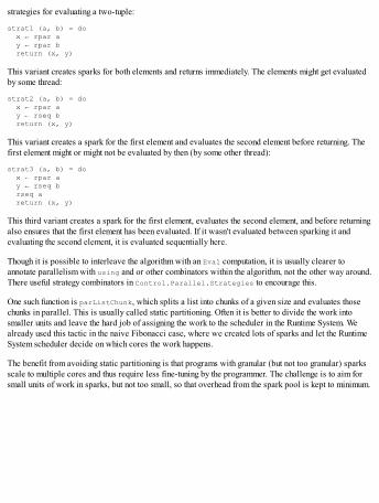
strategies for evaluating a two-tuple:

strat1 (a, b) = do x ← rpar a y ← rpar b return (x, y)

This variant creates sparks for both elements and returns immediately. The elements might get evaluatedby some thread:

strat2 (a, b) = do x ← rpar a y ← rseq b return (x, y)

This variant creates a spark for the first element and evaluates the second element before returning. Thefirst element might or might not be evaluated by then (by some other thread):

strat3 (a, b) = do x ← rpar a y ← rseq b rseq a return (x, y)

This third variant creates a spark for the first element, evaluates the second element, and before returningalso ensures that the first element has been evaluated. If it wasn't evaluated between sparking it andevaluating the second element, it is evaluated sequentially here.

Though it is possible to interleave the algorithm with an Eval computation, it is usually clearer toannotate parallelism with using and or other combinators within the algorithm, not the other way around.There useful strategy combinators in Control.Parallel.Strategies to encourage this.

One such function is parListChunk, which splits a list into chunks of a given size and evaluates thosechunks in parallel. This is usually called static partitioning. Often it is better to divide the work intosmaller units and leave the hard job of assigning the work to the scheduler in the Runtime System. Wealready used this tactic in the naive Fibonacci case, where we created lots of sparks and let the RuntimeSystem scheduler decide on which cores the work happens.

The benefit from avoiding static partitioning is that programs with granular (but not too granular) sparksscale to multiple cores and thus require less fine-tuning by the programmer. The challenge is to aim forsmall units of work in sparks, but not too small, so that overhead from the spark pool is kept to minimum.

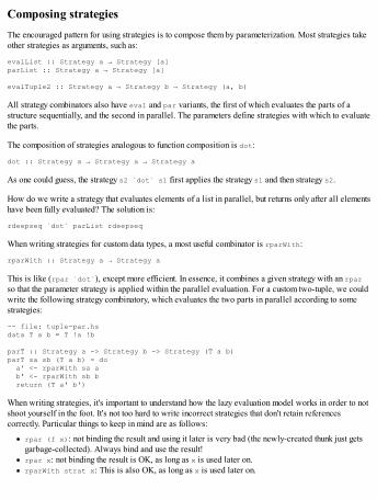
Composing strategiesThe encouraged pattern for using strategies is to compose them by parameterization. Most strategies takeother strategies as arguments, such as:

evalList :: Strategy a → Strategy [a]parList :: Strategy a → Strategy [a]

evalTuple2 :: Strategy a → Strategy b → Strategy (a, b)

All strategy combinators also have eval and par variants, the first of which evaluates the parts of astructure sequentially, and the second in parallel. The parameters define strategies with which to evaluatethe parts.

The composition of strategies analogous to function composition is dot:

dot :: Strategy a → Strategy a → Strategy a

As one could guess, the strategy s2 `dot` s1 first applies the strategy s1 and then strategy s2.

How do we write a strategy that evaluates elements of a list in parallel, but returns only after all elementshave been fully evaluated? The solution is:

rdeepseq `dot` parList rdeepseq

When writing strategies for custom data types, a most useful combinator is rparWith:

rparWith :: Strategy a → Strategy a

This is like (rpar `dot`), except more efficient. In essence, it combines a given strategy with an rparso that the parameter strategy is applied within the parallel evaluation. For a custom two-tuple, we couldwrite the following strategy combinatory, which evaluates the two parts in parallel according to somestrategies:

-- file: tuple-par.hsdata T a b = T !a !b

parT :: Strategy a -> Strategy b -> Strategy (T a b)parT sa sb (T a b) = do a' <- rparWith sa a b' <- rparWith sb b return (T a' b')

When writing strategies, it's important to understand how the lazy evaluation model works in order to notshoot yourself in the foot. It's not too hard to write incorrect strategies that don't retain referencescorrectly. Particular things to keep in mind are as follows:

rpar (f x): not binding the result and using it later is very bad (the newly-created thunk just getsgarbage-collected). Always bind and use the result!rpar x: not binding the result is OK, as long as x is used later on.rparWith strat x: This is also OK, as long as x is used later on.

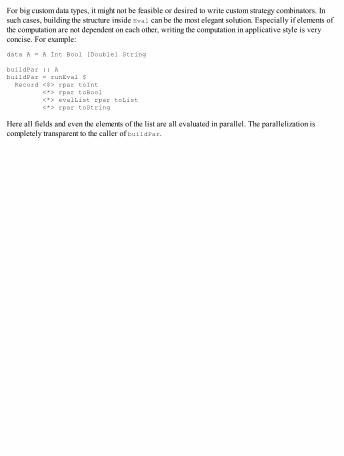
For big custom data types, it might not be feasible or desired to write custom strategy combinators. Insuch cases, building the structure inside Eval can be the most elegant solution. Especially if elements ofthe computation are not dependent on each other, writing the computation in applicative style is veryconcise. For example:

data A = A Int Bool [Double] String

buildPar :: AbuildPar = runEval $ Record <$> rpar toInt <*> rpar toBool <*> evalList rpar toList <*> rpar toString

Here all fields and even the elements of the list are all evaluated in parallel. The parallelization iscompletely transparent to the caller of buildPar.

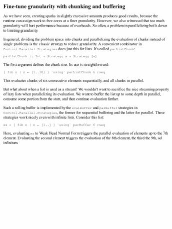
Fine-tune granularity with chunking and bufferingAs we have seen, creating sparks in slightly excessive amounts produces good results, because theruntime can assign work to free cores at a finer granularity. However, we also witnessed that too muchgranularity will hurt performance because of overheads. So often, a problem in parallelizing boils downto limiting granularity.

In general, dividing the problem space into chunks and parallelizing the evaluation of chunks instead ofsingle problems is the classic strategy to reduce granularity. A convenient combinator inControl.Parallel.Strategies does just this for lists. It's called parListChunk:

parListChunk :: Int → Strategy a → Strategy [a]

The first argument defines the chunk size. Its use is straightforward:

[ fib n | n ← [1..30] ] `using` parListChunk 6 rseq

This evaluates chunks of six consecutive elements sequentially, and all chunks in parallel.

But what about when a list is used as a stream? We wouldn't want to sacrifice the nice streaming propertyof lazy lists when parallelizing its evaluation. We want to buffer the list up to some depth in parallel,consume some portion from the start, and then continue evaluation further.

Such a rolling buffer is implemented by the evalBuffer and parBuffer strategies inControl.Parallel.Strategies, the former for sequential buffering and the latter for parallel. Thesestrategies work nicely even with infinite lists. Consider this list:

xs = [ fib n | n ← [1..] ] `using` parBuffer 6 rseq

Here, evaluating xs to Weak Head Normal Form triggers the parallel evaluation of elements up to the 7thelement. Evaluating the second element triggers the evaluation of the 8th element, the third the 9th, adinfinitum.

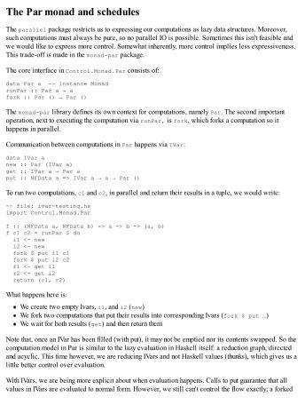
The Par monad and schedulesThe parallel package restricts us to expressing our computations as lazy data structures. Moreover,such computations must always be pure, so no parallel IO is possible. Sometimes this isn't feasible andwe would like to express more control. Somewhat inherently, more control implies less expressiveness.This trade-off is made in the monad-par package.

The core interface in Control.Monad.Par consists of:

data Par a -- instance MonadrunPar :: Par a → afork :: Par () → Par ()

The monad-par library defines its own context for computations, namely Par. The second importantoperation, next to executing the computation via runPar, is fork, which forks a computation so ithappens in parallel.

Communication between computations in Par happens via IVar:

data IVar anew :: Par (IVar a)get :: IVar a → Par aput :: NFData a => IVar a → a → Par ()

To run two computations, c1 and c2, in parallel and return their results in a tuple, we would write:

-- file: ivar-testing.hsimport Control.Monad.Par

f :: (NFData a, NFData b) => a -> b -> (a, b)f c1 c2 = runPar $ do i1 <- new i2 <- new fork $ put i1 c1 fork $ put i2 c2 r1 <- get i1 r2 <- get i2 return (r1, r2)

What happens here is:

We create two empty Ivars, i1, and i2 (new)We fork two computations that put their results into corresponding Ivars (fork $ put …)We wait for both results (get) and then return them

Note that, once an IVar has been filled (with put), it may not be emptied nor its contents swapped. So thecomputation model in Par is similar to the lazy evaluation in Haskell itself: a reduction graph, directedand acyclic. This time however, we are reducing IVars and not Haskell values (thunks), which gives us alittle better control over evaluation.

With IVars, we are being more explicit about when evaluation happens. Calls to put guarantee that allvalues in IVars are evaluated to normal form. However, we still can't control the flow exactly; a forked

Par action may be executed anywhere between the call to fork and get, which requires a value from aforked Par. But with pure values, the result is always deterministic.

The dataflow-style of parallel programming that monad-par encourages is better suited for someapplications, whereas the strategy-style parallel evaluation of lazy data structures is better for others.

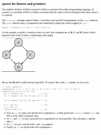
spawn for futures and promisesYou might be familiar with the concept of a future or promise from other programming languages. Inessence, we can think of IVar as a future or promise that the value will be calculated at the latest when itis required.

The monad-par package supports future- or promise-style parallel programming via the spawn function.The spawn function takes a computation and immediately returns the result wrapped in IVar:

spawn :: NFData a => Par a → Par (IVar a)

For the moment, consider a situation where we have four computations A, B, C, and D. Some of themdepend on the result of others, conforming to this graph:

We see that B and C could execute in parallel. To express this in the Par monad, we can write:

-- file: spawn.hscomputation :: A -> (A -> B) -> (A -> C) -> (B -> C -> D) -> Par Dcomputation fa fb fc fd = do av <- newFull fa -- (1) bv <- spawn $ do fb <$> get av -- (2)

cv <- spawn $ do fc <$> get av -- (3)

b <- get bv -- (4) c <- get cv return (fd b c) -- (5)

First, at (1) we make sure that the first computation A is fully performed. newFull creates IVar andfills it with a fully evaluated value.At (2) and (3), we have spawned two computations to run in parallel. One calculates B and theother C.At (4), we now wait for both B and C to complete.Finally, at (5) we perform the last computation D.

Non-deterministic parallelism with ParIOWhat if the computations A, B, C, and D involved IO? The IO module from monad-par,Control.Monad.Par.IO, provides another monad for parallel IO: ParIO.

ParIO is largely similar to Par, except that it allows lifting IO operations into it. IO also brings with itsome non-determinism over pure Par.

With ParIO, we cannot use the same functions that worked with pure Par. We need to use the overloadedAPI from the abstract-par package. The function names stay the same with the overloaded API, so it'sno big deal – really a drop-in replacement (for pure Par too).

Let's see how we would write our A, B, C, D computation in terms of IO actions. The required importschange from one import to three:

import Control.Monad.IO.Classimport Control.Monad.Par.IOimport Control.Monad.Par.Class

From the first module, we need only liftIO to perform IO actions in ParIO. The second module gives usthe ParIO type. The last one is the overloaded Par API.

The computation itself doesn't change much:

-- file: spawnio.hscomputationIO :: IO A -> (A -> IO B) -> (A -> IO C) -> (B -> C -> IO D) -> ParIO DcomputationIO fa fb fc fd = do av <- newFull =<< liftIO fa bv <- spawn $ liftIO . fb =<< get av

cv <- spawn $ liftIO . Fc =<< get av

b <- get bv c <- get cv liftIO (fd b c)

Basically we just plugged in some liftIO here and there. Bear in mind that the only order enforced onIO actions is due to calls to put and get; an IO action may be performed whenever all IVar datadependencies before it have been met. So when doing impure parallelism, ensure that I/O actions interactwith each other only via IVars to prevent unexpected behavior.

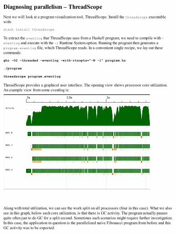
Diagnosing parallelism – ThreadScopeNext we will look at a program visualization tool, ThreadScope. Install the threadscope executablewith:

stack install threadscope

To extract the eventlog that ThreadScope uses from a Haskell program, we need to compile with -eventlog and execute with the -l Runtime System option. Running the program then generates aprogram.eventlog file, which ThreadScope reads. In a convenient single recipe, we lay out thesecommands:

ghc -O2 -threaded -eventlog -with-rtsopts="-N -l" program.hs

./program

threadscope program.eventlog

ThreadScope provides a graphical user interface. The opening view shows processor core utilization.An example view from some eventlog is:

Along with total utilization, we can see the work split on all processors (four in this case). What we alsosee in this graph, below each core utilization, is that there is GC activity. The program actually pausesquite often just to do GC for a split second. Sometimes such scenarios might require further investigation.In this case, the application in question is the parallelized naive Fibonacci program from before and thisGC activity was to be expected.

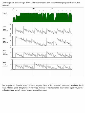
Other things that ThreadScope shows us include the spark pool sizes over the program's lifetime. Forexample:

This is again data from the naive Fibonacci program. Most of the time there's some work available for allcores, which is good. The graph is rather rough because of the exponential nature of the algorithm, so thisis about as good a spark rate as we can reasonably expect.

Data parallel programming – RepaRepa (regular parallel) is a Haskell library providing regular parallel arrays. Repa performs very wellin image processing, for example. Doing computations on large data structures in parallel is Repa'sspecialty. Repa is installed with:

stack install repa

The parts on Repa in this chapter are written for version 3.4.0.2 of the Repa library. The main interface isexported by the Data.Array.Repa module.

At first glance, the library perhaps looks a bit complex. For instance, the parallel sum function has thisdaunting type signature:

sumAllP:: (Shape sh, Source r a, Elt a, Unbox a, Num a, Monad m)=> Array r sh a -> m a

Repa uses a lot of classes to overload functionality over different types of array. The type of immutablearrays in Repa contains three type variables:

data Array r sh e

Here, r defines representation, sh defines shape, and e defines the array elements' type. For example, aone-dimensional array of unboxed Int is given by:

Array U DIM1 Int

Mutable arrays in Repa can be represented by another type, MVec r e. The difference with immutablearrays is that mutable arrays don't have a defined shape; they're always linear or one-dimensional. Butrarely is it necessary to use explicitly mutable arrays thanks to Repa's fusion system.

Playing with Repa in GHCiLet's fire up GHCi to get the hang of the Repa library. A one-dimensional array of unboxed Ints isconstructed from a list with the fromListUnboxed function:

> import Data.Array.Repa as Repa> let x = fromListUnboxed (ix1 3) [0, 1, 2 :: Int]> :t xx :: Array U DIM1 Int

Many definitions from Repa overlap with definitions from Prelude, so we want a shorthand qualifier forthe Repa library. Then, when building a list, note that we had to provide fromListUnboxed with theexact size or shape of the resulting array. The recommended way to construct shape definitions is with theix1, ix2, and ix3 functions.

Repa arrays are shape-polymorphic, but not shape-agnostic; Repa is actually quite strict about aligningshapes correctly in computations. On the type level, we are guaranteed that the number of dimensionswill match or else there will be a type error. Constructing two-dimensional arrays is straightforward:

> let y = fromListUnboxed (ix2 2 2) [1, 1, 1, 0 :: Int]> yAUnboxed ((Z :. 2) :. 2) [1,1,1,0]

Here, we witness the show instance for unboxed arrays. Conforming read instances are of course alsoprovided. The specialized data type under the array abstraction leaks a little, in a sense. AUnboxed is theconcrete data type for unboxed vectors whereas array r sh e is in fact an (associated) type family, or inclearer terms just a function on the type level. So although array is not really a data type itself, in practiceit can be thought of as one.

We can retrieve the shape of any Repa array as a value with the extent function:

> extent y(Z :. 2) :. 2

Indexing into Repa arrays happens with the (!) operator. The index is given as a shape of the same typeas the array's extent. For instance:

> y ! ix2 1 01

Mapping and delayed arrays

We can map over the elements in the functor style with Repa.map:

map :: (Shape sh, Source r a) → (a → b) → Array r sh a → Array D sh b

Looking at the type of map, we see that, whatever representation the argument array uses, therepresentation of the resulting array is always D for delayed. In the delayed array representation, eachelement is given as a function in a sense. Indexing works normally for delayed arrays (the work related tocalculating the element is done on-demand):

> Repa.map (+10) x ! ix1 111

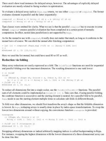
There aren't show/read instances for delayed arrays, however. The advantages of explicitly delayedevaluation are mostly related to fusing workers in optimization.

To evaluate a delayed array such as Repa.map returns, we use either computeP or computeS. The formerevaluates elements in parallel and the latter sequentially:

computeP :: Monad m => Array r1 sh e → m (Array r2 sh e)computeS :: Array r1 sh e → Array r2 sh e

Type classes were omitted for clarity. What we see is that the parallel computeP has to execute in somemonad. computeP ensures parallel evaluation has been completed at a certain point of monadiccomputation. In effect, nested data parallelism is not supported by Repa.

As for the monad to use with computeP, it really does not matter that much, as long as it conforms to themonad laws of course. We can ditch the monad after finishing computation:

> let [r] = computeP (Repa.map (+10) x) :: [Array U DIM1 Int]> rAUnboxed (Z :. 3) [10,11,12]

Here we used the list monad, but could have used IO or ST as well.

Reduction via folding

Many array reductions are easily expressed as a fold. The foldS/foldP functions are used for sequentialand parallel folding over the innermost dimension. The resulting dimension is one rank lower:

> :t foldPfoldP :: (Monad m, Shape sh, Source r a, Unbox a, Elt a) => (a -> a -> a) -> a -> Array r (sh :. Int) a ->m (Array U sh a)> foldP (+) 0 yAUnboxed (Z :. 2) [2,1]

To reduce all dimensions flat into a single scalar, use the foldAllS/foldAllP functions. The parallelsum of all elements could be implemented as foldAllP (+) 0. Take care that, if using parallel folding,the combiner function is associative and the starting element is neutral; for a parallel fold to be parallel,Repa needs to use the starting element multiple times to calculate sub-folds in different threads.

To fold over other dimensions, we should first transform the array's shape so that the foldable dimensionis lowest. In Repa, reshaping arrays is usually done in place by index-space transformations. To swap thelowest two dimensions around without copying, the convenience function transpose is provided:

transpose :: (Shape sh, Source r e) => Array r ((sh :. Int) :. Int) e -> Array D ((sh :. Int) :. Int) e

> foldP (+) 0 (transpose y)AUnboxed (Z :. 2) [2,1]

Swapping arbitrary dimensions or indeed arbitrarily mapping indices is called backpermuting in Repa.For instance, swapping the highest dimension with the lowest dimension of a three-dimensional array canbe done like this:

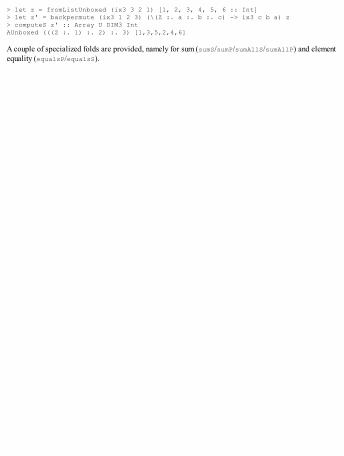
> let z = fromListUnboxed (ix3 3 2 1) [1, 2, 3, 4, 5, 6 :: Int]> let z' = backpermute (ix3 1 2 3) (\(Z :. a :. b :. c) -> ix3 c b a) z> computeS z' :: Array U DIM3 IntAUnboxed (((Z :. 1) :. 2) :. 3) [1,3,5,2,4,6]

A couple of specialized folds are provided, namely for sum (sumS/sumP/sumAllS/sumAllP) and elementequality (equalsP/equalsS).

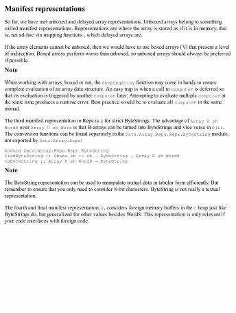
Manifest representationsSo far, we have met unboxed and delayed array representations. Unboxed arrays belong to somethingcalled manifest representations. Representations are where the array is stored as if it is in memory, thatis, not ad-hoc via mapping functions , which delayed arrays are.

If the array elements cannot be unboxed, then we would have to use boxed arrays (V) that present a levelof indirection. Boxed arrays perform worse than unboxed, so unboxed arrays should always be preferredif possible.

Note

When working with arrays, boxed or not, the deepSeqArray function may come in handy to ensurecomplete evaluation of an array data structure. An easy trap is when a call to computeP is deferred sothat its evaluation is triggered by another computeP later. Attempting to evaluate multiple computeP atthe same time produces a runtime error. Best practice would be to evaluate all computeP in the samemonad.

The third manifest representation in Repa is B for strict ByteStrings. The advantage of Array B shWord8 over Array U sh Word is that B-arrays can be turned into ByteStrings and vice versa in O(1).The conversion functions can be found separately in the Data.Array.Repa.Repr.ByteString module,not exported by Data.Array.Repa:

module Data.Array.Repa.Repr.ByteStringfromByteString :: Shape sh => sh → ByteString → Array B sh Word8toByteString :: Array B sh Word8 → ByteString

Note

The ByteString representation can be used to manipulate textual data in tabular form efficiently. Butremember to ensure that you only need to consider 8-bit characters. ByteString is not really a textualrepresentation.

The fourth and final manifest representation, F, considers foreign memory buffers in the C heap just likeByteStrings do, but generalized for other values besides Word8. This representation is only relevant ifyour code interfaces with foreign code.

Delayed representation and fusionAlong with manifest representations are delayed representations. The first delayed representation, D,presents elements as functions from indices to elements. Most combinators in Repa return arrays in adelayed representation. This is because we can eliminate a lot of intermediate arrays, for instance,mapping twice like in:

computeS . Repa.map (+ 1) . Repa.map (* 2)

Like we would expect from other fusion frameworks, this fuses into a tight loop. The intermediatedelayed array is certainly eliminated when compiling. In a way, the fusion framework in Repa gives usmore control over when fusion happens. This is nice because it makes it easy to predict the performanceof Repa programs. Although our code looks like we are operating on immutable arrays, constructing themover and over again, in practice correctly written Repa programs will optimize very nicely into fastcode.

Note

Using computeS/computeP quite often requires an explicit type signature, because the target array ispolymorphic in its representation (either unboxed array, boxed array, or foreign buffer). Usually unboxedarray is the desired choice, for which more specific functions, computeUnboxedP andcomputeUnboxedS, provide specialized type readily.

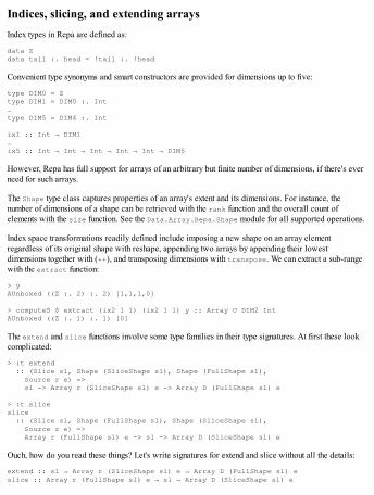
Indices, slicing, and extending arraysIndex types in Repa are defined as:

data Zdata tail :. head = !tail :. !head

Convenient type synonyms and smart constructors are provided for dimensions up to five:

type DIM0 = Ztype DIM1 = DIM0 :. Int…type DIM5 = DIM4 :. Int

ix1 :: Int → DIM1…ix5 :: Int → Int → Int → Int → Int → DIM5

However, Repa has full support for arrays of an arbitrary but finite number of dimensions, if there's everneed for such arrays.

The Shape type class captures properties of an array's extent and its dimensions. For instance, thenumber of dimensions of a shape can be retrieved with the rank function and the overall count ofelements with the size function. See the Data.Array.Repa.Shape module for all supported operations.

Index space transformations readily defined include imposing a new shape on an array elementregardless of its original shape with reshape, appending two arrays by appending their lowestdimensions together with (++), and transposing dimensions with transpose. We can extract a sub-rangewith the extract function:

> yAUnboxed ((Z :. 2) :. 2) [1,1,1,0]

> computeS $ extract (ix2 1 1) (ix2 1 1) y :: Array U DIM2 IntAUnboxed ((Z :. 1) :. 1) [0]

The extend and slice functions involve some type families in their type signatures. At first these lookcomplicated:

> :t extend :: (Slice sl, Shape (SliceShape sl), Shape (FullShape sl), Source r e) => sl -> Array r (SliceShape sl) e -> Array D (FullShape sl) e

> :t sliceslice :: (Slice sl, Shape (FullShape sl), Shape (SliceShape sl), Source r e) => Array r (FullShape sl) e -> sl -> Array D (SliceShape sl) e

Ouch, how do you read these things? Let's write signatures for extend and slice without all the details:

extend :: sl → Array r (SliceShape sl) e → Array D (FullShape sl) eslice :: Array r (FullShape sl) e → sl → Array D (SliceShape sl) e

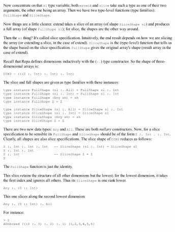
Now concentrate on that sl type variable; both extend and slice take such a type as one of their twoarguments, the other one being an array. Then we have two type-level functions (type families):FullShape and SliceShape.

Now things are a little clearer. extend takes a slice of an array (of shape SliceShape sl) and producesa full array (of shape FullShape sl); for slice, the shapes are the other way around.

Then the sl thing? It's called slice specification. Intuitively, the end result depends on how we are slicingthe array (or extending a slice, in the case of extend). SliceShape is the (type-level) function that tells usthe shape based on the slice specification. FullShape gives the original array's shape (result array in thecase of extend).

Recall that Repa defines dimensions inductively with the (:.) type constructor. So the shape of three-dimensional arrays is:

DIM3 ~ (((Z :. Int) :. Int) :. Int)

The slice and full shapes are given as type families with these instances:

type instance FullShape (sl :. All) = FullShape sl :. Inttype instance FullShape (sl :. Int) = FullShape sl :. Inttype instance FullShape (Any sh) = shtype instance FullShape Z = Z

type instance SliceShape (sl :. All) = SliceShape sl :. Inttype instance SliceShape (sl :. Int) = SliceShape sltype instance SliceShape (Any sh) = shtype instance SliceShape Z = Z

There are two new data types: Any and All. These are both nullary constructors. Now, for a slicespecification to be sensible its FullShape and SliceShape should be of the form Z :. Int … :. Int.Clearly, all shapes are also slice specifications. The slice shape of DIM3 reduces as follows:

Z :. Int :. Int :. Int -- SliceShape (sl :. Int) = SliceShape slZ :. Int :. IntZ :. Int -- SliceShape Z = ZZ

The FullShape function is just the identity.

This slice retains the structure of all other dimensions but the lowest; for the lowest dimension, it takesthe first index and ignores all others. Thus its SliceShape is one rank lower.

Any :. (0 :: Int)

This one slices along the second lowest dimension:

Any :. (0 :: Int) :. All

For instance:

> zAUnboxed (((Z :. 3) :. 2) :. 1) [1,2,3,4,5,6]

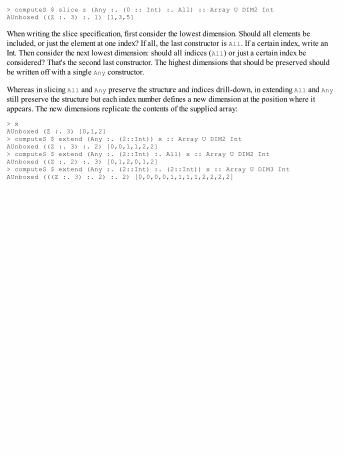
> computeS $ slice z (Any :. (0 :: Int) :. All) :: Array U DIM2 IntAUnboxed ((Z :. 3) :. 1) [1,3,5]

When writing the slice specification, first consider the lowest dimension. Should all elements beincluded, or just the element at one index? If all, the last constructor is All. If a certain index, write anInt. Then consider the next lowest dimension: should all indices (All) or just a certain index beconsidered? That's the second last constructor. The highest dimensions that should be preserved shouldbe written off with a single Any constructor.

Whereas in slicing All and Any preserve the structure and indices drill-down, in extending All and Anystill preserve the structure but each index number defines a new dimension at the position where itappears. The new dimensions replicate the contents of the supplied array:

> xAUnboxed (Z :. 3) [0,1,2]> computeS $ extend (Any :. (2::Int)) x :: Array U DIM2 IntAUnboxed ((Z :. 3) :. 2) [0,0,1,1,2,2]> computeS $ extend (Any :. (2::Int) :. All) x :: Array U DIM2 IntAUnboxed ((Z :. 2) :. 3) [0,1,2,0,1,2]> computeS $ extend (Any :. (2::Int) :. (2::Int)) x :: Array U DIM3 IntAUnboxed (((Z :. 3) :. 2) :. 2) [0,0,0,0,1,1,1,1,2,2,2,2]

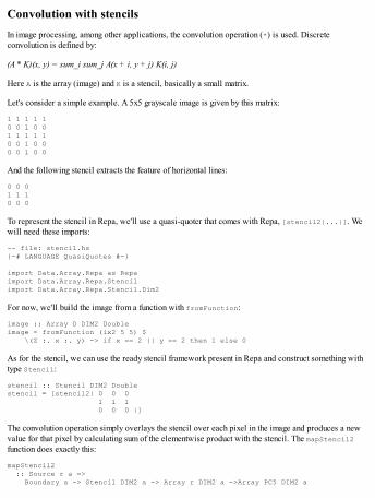
Convolution with stencilsIn image processing, among other applications, the convolution operation (*) is used. Discreteconvolution is defined by:

(A * K)(x, y) = sum_i sum_j A(x + i, y + j) K(i, j)

Here A is the array (image) and K is a stencil, basically a small matrix.

Let's consider a simple example. A 5x5 grayscale image is given by this matrix:

1 1 1 1 10 0 1 0 01 1 1 1 10 0 1 0 00 0 1 0 0

And the following stencil extracts the feature of horizontal lines:

0 0 01 1 10 0 0

To represent the stencil in Repa, we'll use a quasi-quoter that comes with Repa, [stencil2|...|]. Wewill need these imports:

-- file: stencil.hs{-# LANGUAGE QuasiQuotes #-}

import Data.Array.Repa as Repaimport Data.Array.Repa.Stencilimport Data.Array.Repa.Stencil.Dim2

For now, we'll build the image from a function with fromFunction:

image :: Array D DIM2 Doubleimage = fromFunction (ix2 5 5) $ \(Z :. x :. y) -> if x == 2 || y == 2 then 1 else 0

As for the stencil, we can use the ready stencil framework present in Repa and construct something withtype Stencil:

stencil :: Stencil DIM2 Doublestencil = [stencil2| 0 0 0 1 1 1 0 0 0 |]

The convolution operation simply overlays the stencil over each pixel in the image and produces a newvalue for that pixel by calculating sum of the elementwise product with the stencil. The mapStencil2function does exactly this:

mapStencil2 :: Source r a => Boundary a -> Stencil DIM2 a -> Array r DIM2 a ->Array PC5 DIM2 a

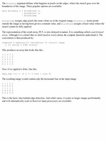
The Boundary argument defines what happens at pixels on the edges, where the stencil goes over theboundaries of the image. Three popular options are available:

data Boundary a = BoundFixed !a | BoundConst !a | BoundClamp

BoundClamp assigns edge pixels the same values as in the original image, BoundConst treats pointsoutside the image as having been given a constant value, and BoundFixed assigns a fixed value where thestencil cannot be fully applied.

The representation of the result array, PC5, is also delayed in nature. It is something called a partitionedarray. Although it is a detail that we don't need to worry about, the compute functions understand it. Theconvolution is then produced by:

computeP $ mapStencil2 (BoundConst 0) stencil image :: IO (Array U DIM2 Double)

This produces an array that looks like this:

3 3 3 3 30 1 1 1 03 3 3 3 30 1 1 1 00 1 1 1 0

Now if we applied a filter, like this:

Repa.map (\x -> if x >= 3 then 1 else 0)

The resulting image would contain only the horizontal line in the input image:

1 1 1 1 10 0 0 0 01 1 1 1 10 0 0 0 00 0 0 0 0

This is the basic idea behind edge detection. And what's more, it scales to larger images performantlyand will automatically scale to however many processors are available.

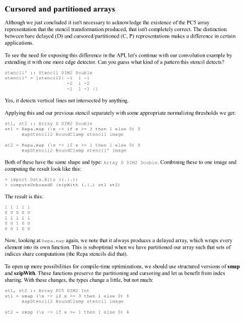
Cursored and partitioned arraysAlthough we just concluded it isn't necessary to acknowledge the existence of the PC5 arrayrepresentation that the stencil transformation produced, that isn't completely correct. The distinctionbetween bare delayed (D) and cursored/partitioned (C, P) representations makes a difference in certainapplications.

To see the need for exposing this difference in the API, let's continue with our convolution example byextending it with one more edge detector. Can you guess what kind of a pattern this stencil detects?

stencil' :: Stencil DIM2 Doublestencil' = [stencil2| -1 1 -1 -2 1 -2 -1 1 -1 |]

Yes, it detects vertical lines not intersected by anything.

Applying this and our previous stencil separately with some appropriate normalizing thresholds we get:

st1, st2 :: Array D DIM2 Doublest1 = Repa.map (\x -> if x >= 3 then 1 else 0) $ mapStencil2 BoundClamp stencil image

st2 = Repa.map (\x -> if x >= 1 then 1 else 0) $ mapStencil2 BoundClamp stencil' image

Both of these have the same shape and type: Array D DIM2 Double. Combining these to one image andcomputing the result look like this:

> import Data.Bits ((.|.))> computeUnboxedP (zipWith (.|.) st1 st2)

The result is this:

1 1 1 1 10 0 0 0 01 1 1 1 10 0 1 0 00 0 1 0 0

Now, looking at Repa.map again, we note that it always produces a delayed array, which wraps everyelement into its own function. This is suboptimal when we have partitioned our array such that sets ofindices share computations (the Repa stencils did that).

To open up more possibilities for compile-time optimizations, we should use structured versions of smapand szipWith. These functions preserve the partitioning and cursoring and let us benefit from indexsharing. With these changes, the types change a little, but not much:

st1, st2 :: Array PC5 DIM2 Intst1 = smap (\x -> if x >= 3 then 1 else 0) $ mapStencil2 BoundClamp stencil image

st2 = smap (\x -> if x >= 1 then 1 else 0) $

mapStencil2 BoundClamp stencil' image

> print $ computeUnboxedS $ szipWith (.|.) st1 st2

Writing fast Repa codeThere are numerous tricks for writing fast and well-parallelizing code with Repa. Enumerating from mostimportant to least important, we have:

Vectorize: Work the algorithm such that as much as possible is done with array operations. Useunboxed arrays unless you have a good reason not to.Compute only where necessary: The more delayed arrays there are, the more fusion will likelytake place and the produced code will be faster. Unless not evaluating would take up too muchmemory, it is usually best to defer it further. Computation usually creates a new manifest array.Parallelize with optimal granularity: Using parallel computeP, foldP, and others is faster onbigger arrays or with a bigger bunch of work; for little work, computeS and foldS have lessoverhead. The lack of nested parallelism encourages us to lift parallelism to the top level for besteffect.Compile with optimizations, threaded and with LLVM: A good base set of flags for Repaprograms in production is -Odph -threaded -rtsopts -fllvm -fno-liberate-case -optlo-O3.Bang everything: All lazy arguments and data type fields should be strict.Inline extensively: The fusion system relies heavily on worker functions getting inlined. Instead ofcluttering your code with INLINE pragmas, consider compiling with these flags -funfolding-use-threshold1000 -funfolding-keenness-factor1000. They tell GHC to inline everything. Thismight increase binary sizes considerably, so these flags should probably be enabled on a per-module basis (using the OPTIONS_GHC pragma).Use unsafe versions of Repa functions: The function unsafeIndex and others fromData.Array.Repa.Unsafe should be preferred when correctness is guaranteed. These unsafevariants don't do bounds-checking and cause undefined behavior if used incorrectly. Therefore,unsafe functions shouldn't be used when developing or testing code.

Additional librariesThere are a number of libraries that complement Repa:

repa-devil: Load and write arrays as image files. Apparently this has been deprecated in favor ofthe friday and friday-devil libraries.repa-io: Load and write arrays in bitmap, binary, ASCII matrix, and vector formats.repa-algorithms: Quite performant implementations of algorithms for matrix operations, Fouriertransform, randomized arrays, and more flexible convolution functions.repa-stream and repa-flow: Data-parallel streaming libraries built on top of Repa.

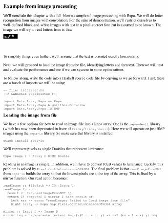
Example from image processingWe'll conclude this chapter with a full-blown example of image processing with Repa. We will do letterrecognition from images with convolution. For the sake of demonstration, we'll restrict ourselves towell-defined black-and-white images with text in a pixel-correct font that is assumed to be known. Theimage we will try to read letters from is this:

To simplify things even further, we'll assume that the text is oriented exactly horizontally.

Next, we will proceed to load the image from the file, identifying letters and then text. Then we will testand evaluate the performance and see if we can squeeze in some optimizations.

To follow along, write the code into a Haskell source code file by copying as we go forward. First, theseare a bunch of imports we will be using:

-- file: letterrec.hs{-# LANGUAGE QuasiQuotes #-}

import Data.Array.Repa as Repaimport Data.Array.Repa.Algorithms.Convolveimport Data.Array.Repa.IO.BMP

Loading the image from file

We have a few options for how to read an image file into a Repa array. One is the repa-devil library(which has now been deprecated in favor of friday/friday-devil). Here we will operate on just BMPimages using the repa-io library. So make sure that library is installed:

stack install repa-io

We'll represent pixels as single Doubles that represent luminance:

type Image r = Array r DIM2 Double

Reading in an image is simple. In addition, we'll have to convert RGB values to luminance. Luckily, thisproblem is solved by Pixel.doubleLuminanceOfRGB8. The final problem is that readImageFromBMPfrom repa-io builds the array so that the lowest pixels are at the top of the array. This is fixed by amirror function. Our read action becomes:

readImage :: FilePath -> IO (Image U)readImage fp = do result <- BMP.readImageFromBMP fp return $! computeS $ mirror $ case result of Left err -> error "readImage: Failed to load image from file" Right array -> Repa.map Pixel.doubleLuminanceOfRGB8 array

mirror :: Image D -> Image Dmirror img = backpermute (extent img)(\(Z :. x :. y) -> ix2 (mx - 1 - x) y) img

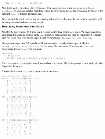
where Z :. mx :. _ = extent img

Note that I used ($!) instead of ($). This way, if the image file was faulty, we get an error beforereadImage IO action completes. With lazy return, the error would be silently propagated to wherever thereturned Image D thunk is next requested.

We computed the result here instead of returning a delayed array because the convolution operation we'llbe using expects an unboxed array as input.

Identifying letters with convolution

Next for the convolution. We'll implement recognition for three letters: a, b, and c. We make stencils foreach letter. But using the stencils in the repa library is not an option this time, because letter b is largerthan 7x7 in our font, which is the upper bound on stencil size in Data.Array.Repa.Stencil.

To represent larger than 7x7 stencils, we'll again resort to repa-algorithms, specifically theData.Array.Repa.Algorithms.Convolve module. The function we'll be using is convolveP.Specialized for our Image type, we have:

convoleP :: Monad m => (DIM2 → Double) → Image U → Image U → m (Image U)

This convolution represents the stencil as an unboxed array too. The first argument is used to decide whathappens at the edges.

The stencils for letters a, b, and c in our font are therefore:

sta, stb, stc :: Image Usta = fromListUnboxed (ix2 6 5) [ -1, 1, 1, 1, -1 , -1, -1, -1, -1, 1 , -1, 1, 1, 1, 1 , 1, -1, -1, -1, 1 , 1, -1, -1, -1, 1 , -1, 1, 1, 1, 1 ]

stb = fromListUnboxed (ix2 8 5) [ 1, -1, -1, -1, -1 , 1, -1, -1, -1, -1 , 1, 1, 1, 1, -1 , 1, -1, -1, -1, 1 , 1, -1, -1, -1, 1 , 1, -1, -1, -1, 1 , 1, -1, -1, -1, 1 , 1, 1, 1, 1, -1 ]

stc = fromListUnboxed (ix2 6 5) [ -1, 1, 1, 1, -1 , 1, -1, -1, -1, 1 , 1, -1, -1, -1, -1 , 1, -1, -1, -1, -1 , 1, -1, -1, -1, 1 , -1, 1, 1, 1, -1 ]

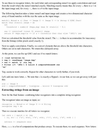
To use these to recognize letters, for each letter and corresponding stencil we apply convolution and readfrom the result where the stencil matched exactly. Matching exactly means that, for every 1, there is a 1 inthe input image and, for every -1, there is a 0 in the input image.

The following function takes a letter stencil and input image and creates a two-dimensional characterarray of found matches with the size the same as the input image:

match:: Monad m => Char -> Image U -> Image U -> m (Array D DIM2 Char)match char stencil image = do let threshold = sumAllS (Repa.map (max 0) stencil) – 0.1

res <- convolveP (const 0) stencil image return $! Repa.map(\x -> if x > threshold then char else '\NUL') res

First we calculated the threshold value from the stencil. The 0.1 is there to accommodate for inaccuracyfrom the bitmap (white pixels aren't exactly 1).

Next we apply convolution. Finally, we convert elements that are above the threshold into characters.Others are set to null characters. We return this (delayed) array.

At this point, we can fire up GHCi and see if we match letters:

> :load letterrec.hs> img <- readImage "image.bmp"> res <- match 'a' sta img> filter (/= '\NUL') $ toList $ computeUnboxedS res"aa"

Yep, seems to work correctly. Repeat for other characters to verify further, if you wish.

Let's add one more letter, d. We note that d is exactly a flipped b in our font, so we can get away with justthis:

std :: Image Ustd = computeUnboxedS . transpose . mirror $ transpose stb

Extracting strings from an image

Now for the final feature: combining letter recognizers into a complete string recognizer.

The recognizer takes an image as input, so:

recognize :: Monad m => Image U -> m Stringrecognize img = do

Then we execute matches for all letters we recognize:

let recs = [ match c st img | (c, st) ←[ ('a', sta), ('b', stb), ('c', stc), ('d', std) ] ]

letters <- sequence recs

Here, recs is a list of computations that produce arrays. To execute them, we used sequence. Now letters

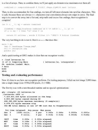
is a list of arrays. Then, to combine them, we'll just apply an element-wise maximum over them all:

combined <- computeUnboxedP $ foldl1 (Repa.zipWith max) letters

Then, to also accommodate for line-endings, we turn all left-most elements into newline characters. Thisis safe, because those are always NUL characters (our convolution always sets edges to zero). The finalstep is to convert the array into a list and, strip nulls and excess line endings; then recognition iscomplete!

let Z :. _ :. my = extent combined

lineEnds = Repa.traverse combined id $ \f ix@(Z :. _ :. y) -> if y == my - 1 then '\n' else f ix

return $! unlines . words $ filter (/= '\NUL') $ toList lineEnds

The very last thing to do is test it. Here's a main that does this:

main = do img <- readImage "image.bmp" str <- recognize img putStr str

And a quick testing at GHCi makes it clear that our recognizer works:

> :load letterrec.hs[1 of 1] Compiling Main ( letterrec.hs, interpreted )Ok, modules loaded: Main.> mainbcdcabca

Testing and evaluating performance

Now it's time to see how our recognizer performs. For testing purposes, I tiled our test image 5,000 timesinto a single image (size 3550x2100 pixels, 21.3 MB).

The first try was with a non-threaded runtime and no special optimizations:

ghc -rtsopts -O3 letterrec.hs./letterrec +RTS -s 7,323,831,024 bytes allocated in the heap 4,803,680 bytes copied during GC 268,385,496 bytes maximum residency (9 sample(s)) 4,978,072 bytes maximum slop 342 MB total memory in use (27 MB lost due to fragmentation)

Tot time (elapsed) Avg pause Max pause Gen 0 13281 colls, 0 par 0.045s 0.044s 0.0000s 0.0001s Gen 1 9 colls, 0 par 0.016s 0.016s 0.0018s 0.0146s

INIT time 0.000s ( 0.000s elapsed) MUT time 9.158s ( 9.172s elapsed) GC time 0.061s ( 0.059s elapsed) EXIT time 0.015s ( 0.015s elapsed)

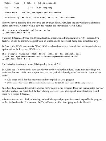
Total time 9.238s ( 9.246s elapsed)

%GC time 0.7% (0.6% elapsed)

Alloc rate 799,722,664 bytes per MUT second

Productivity 99.3% of total user, 99.3% of total elapsed

Now we have a baseline from which we can try to get faster. Next, let's see how well parallelizationaffects the results. Compile with a threaded runtime and run on three system cores:

ghc -rtsopts -threaded -O3 letterrec.hs./letterrec +RTS -N4 -s

The main differences from a non-threaded runtime were: elapsed time reduced to 4.4s (speedup by afactor of 2) and the memory footprint went up a little, due to more work being done simultaneously.

Let's next add LLVM into the mix. With LLVM, we should use -Odph instead, because it enables betteroptimizations for Repa and LLVM code:

ghc -rtsopts -threaded -Odph -fllvm -optlo-O3 -fno-liberate-case -funfolding-use-threshold1000 -funfolding-keeness-factor1000./letterrec +RTS -N4 -s

This cuts down runtime to about 3.8s (speedup factor of 2.5).

Last, let's see if we could still have added some code-level optimizations. There are a few things wecould do. But most of the time is spent in convolveP, which is largely out of our control. Anyway, wecould:

Add bangs to all function arguments and use explicit INLINE pragmasUse unsafeTraverse and unsafeBackpermute instead of traverse and backpermute

Together, these account for about 3%-better performance in our program. If we had implemented more ofthe labor and not just handed all the heavy lifting to convolveP, inlining and unsafe functions wouldmake for a bigger difference.

A better alternative to blindly cluttering code with bangs and pragmas is as usual to profile the programto find the bottlenecks. For instance, the ThreadScope profile of our program looks like this:

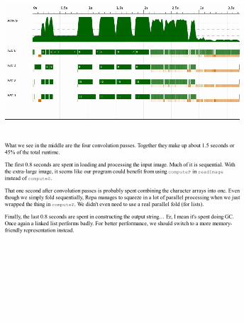
What we see in the middle are the four convolution passes. Together they make up about 1.5 seconds or45% of the total runtime.

The first 0.8 seconds are spent in loading and processing the input image. Much of it is sequential. Withthe extra-large image, it seems like our program could benefit from using computeP in readImageinstead of computeS.

That one second after convolution passes is probably spent combining the character arrays into one. Eventhough we simply fold sequentially, Repa manages to squeeze in a lot of parallel processing when we justwrapped the thing in computeP. We didn't even need to use a real parallel fold (for lists).

Finally, the last 0.8 seconds are spent in constructing the output string… Er, I mean it's spent doing GC.Once again a linked list performs badly. For better performance, we should switch to a more memory-friendly representation instead.

SummaryNow we have crammed in how parallelism is done in Haskell and an overview of the threaded runtime.We parallelized pure and lazy data structures with strategies and Eval (the parallel package). For morecontrol and parallelism in IO, we had to resort to schedules and Par (the monad-par package). We divedinto data-parallel programming with Repa and even wrote a string recognition program with it.

We learned to use the event log and ThreadScope to diagnose the parallel performance of Haskellprograms. Things to keep in mind when parallelizing programs are: use good granularity, not too muchoverhead but not too much sequential processing either; compile with flags optimized for parallelism,especially with Repa; and profile and diagnose before applying transformations at the code level.

In the next chapter, we will look at stream processing in Haskell: I/O, networking, and streaminglibraries such as conduits and pipes. Lazy I/O, combined with interacting with networks, producesnightmarish bugs and sadly it's not easy to get right every time. And the consumer and producer types insome libraries we will look at are scary for sure – but this is just to prevent you from writing incorrectprograms!

Chapter 6. I/O and StreamingI/O in Haskell is a source of confusion for many. The I/O functions in the base library are lazy and allowthe interleaving of I/O side effects with pure code. This produces weird errors at runtime or, even worse,just incorrect behavior without errors. On the other hand, interleaved side-effects allow easy fileprocessing in constant space, among other things. Fortunately, more robust alternatives for streaming havebeen proposed and implemented as libraries.

In this chapter, we will learn to use some of the most popular streaming libraries. But before that, wewill tear down problems with lazy I/O, because it's still often the easiest and most elegant way to do I/O.We will also consider an alternative to lazy I/O, strict I/O.

The I/O we do in this chapter consists of standard input and output, file handles, and network sockets.These cover almost all I/O that's possible in Haskell (we don't do foreign interfaces in this chapter).Resource management is closely related to I/O and so that will be covered too. We will also coverperhaps the most widely seen specific kind of data output ever: writing logs and log files fromapplications. We will look at the following topics:

Working with lazy I/O: recognizing and avoiding problemsTaking care of freeing resources and using ResourceTWorking with streaming libraries: io-streams, pipes, and conduitAdding logging abilities to Haskell applications: fast-logger and monad-logger

Reading, writing, and handling resourcesAlthough it's a common joke that because Haskell is a pure language, we couldn't observe its effects,Haskell actually has very powerful and sophisticated facilities for interacting with the outside world.Besides reading and writing to files and network sockets, I/O affiliates to managing resources thatprovide for input and output.

In this section, we will first point out laziness in Haskell I/O, doing networking with low-level sockets,and consider managing handles and resources.

Traps of lazy I/OLazy I/O allows pure functions to be interleaved with I/O actions arbitrarily. It is important to knowwhen an I/O action defers its action part for later. To demonstrate how easy it is to fall prey to lazy I/O,consider this innocent-looking file manipulation procedure:

-- file: readwrite.hs

main = do writeFile "file.txt" "old" old <- readFile "file.txt" writeFile "file.txt" "new" putStrLn old

However, running this code produces an error at runtime:

readwrite.hs: file.txt: openFile: resource busy (file is locked)

The culprit is readFile, which is lazy in its return value: reading the file begins only when we demandthe results. That would happen on the last line. But readFile does set a lock on the file in the RuntimeSystem immediately, leading to writeFile failing.

Here's another example, using withFile from System.IO to manage the file resource as a file handle:

-- file: readwithfile.hs

import System.IO

main = do old <- withFile "file.txt" ReadWriteMode hGetContents putStrLn old

This time, the runtime error message has more information, as it is associated with a handle instead of afile:

readwithfile.hs: file.txt: hGetContents: illegal operation (delayed read on closed handle)

What's worse, because I/O operations in the base library work with strings, it wouldn't even be enough toseq the result. We would have to do something like seq (last string).

On the other hand, lazy IO and strings allow us to program input and output streams in a similar way tostreaming with pure lists. For example, the echo program in Haskell is simply:

-- file: echo.hsmain = getContents >>= putStr

Or using the interact combinator:

main = interact id

File handles, buffering, and encodingThe Handle data type is used by Runtime System to manage reading and writing from and to filesystemobjects. Standard input, output, and error channels are also handles. These handles are exported inSystem.IO as stdin, stdout, and stderr, respectively. For convenience, basic reading, writing, andappending functions are defined that hide handle opening and closing under the hood. These functionscorrectly close the handle or Handle? make consistent globally even when exceptions are raised.

When working with Handles directly, you are responsible for closing every handle you open. Bestpractice is to use utility functions, such as withFile, that correctly close handles even in the case ofexceptions. With openFile, you are responsible to call hClose on the Handle that openFile returns,preferably using finally or bracket from the Control.Exception module. An example use ofbracket is in the withFile combinator, which we could equally implement ourselves as:

-- file: bracket.hs

import Control.Exceptionimport System.IO hiding (withFile)

withFile :: FilePath -> IOMode -> (Handle -> IO r) -> IO rwithFile file mode go = bracket (openFile file mode) hClose go

Buffering is also controlled via Handles. The preferable buffering mode depends on the application.Three different buffering modes are supported:

BlockBuffering: This is the fastest buffering mode with least overhead, best suited for high-bandwidth applications.LineBuffering: Input and output is handled one line at a time. Best-suited for terminal applications.NoBuffering: Input and output is handled one word or character at a time. This is the only choicefor highly interactive terminal programs, for example. The overhead is very big when processinglarge amounts of data with no buffering.

Basic I/O operations don't bother defining standard buffering modes and instead depend on defaultbuffering of the operating system.

Most of the time the defaults are reasonably sane, such as block-buffering for files and line-buffering forterminal applications. But this isn't always the case: if your application depends on a specific bufferingmode, you should set it yourselves with hSetBuffering. For example, to ensure that a terminalapplication uses line-buffering for both input and output in all cases, we should do something like thefollowing:

-- file: interact.hsimport Data.Char (toUpper)import System.IO

main = do hSetBuffering stdin LineBuffering hSetBuffering stdout LineBuffering interact (map toUpper)

Alongside buffering, text encoding is also a property of handles in text mode. By default, files are always

in text-mode and only opened in non-text or binary mode with openBinaryFile. Encoding is controlledwith hSetEncoding (from System.IO) and, just like with buffering modes, the default encoding dependson the underlaying system's configuration. To set standard input encoding to utf-8, use:

hSetEncoding stdin utf8 :: IO ()

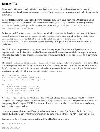
Binary I/OUsing handles in binary mode with functions from System.IO is slightly cumbersome because theinterface is low-level, based on pointers (Ptr a). The bytestring package is usually a better option forbinary I/O.

Recall that ByteStrings came in two flavors: strict and lazy. Both have their own I/O interfaces usingrespective ByteString variants. The I/O interface with bytestring is named consistently with thestring IO interface, using exactly the same names, such as getLine, getContents, interact,readFile, writeFile, and so on.

Before we do I/O with ByteStrings though, we should ensure that the handle we are using is in binarymode. Functions such as withBinaryFile and openBinaryFile take care of this for us. But stdin,stdout, and stderr are by default in text-mode and should be set to binary mode withhSetBinaryMode. This ensures that no special encoding takes place and no newline translation isperformed.

Recall the echo program (echo.hs) we wrote a few pages ago? There is a small problem with thatimplementation: with binary files, end-of-line and end-of-file characters could clutter output in the caseof non-textual data. So in a correct echo program, we should set both stdin and stdout to binary modeat startup.

The strict ByteString from Data.ByteString is always a single, fully evaluated, strict byte array. Thisis to be expected from a strict data structure. But what is not so obvious is that I/O operations with strictByteStrings are also strict. So the write-read-write program that failed with lazy string or String? makeconsistent globally IO will work fine with strict ByteString IO:

-- file: readwrite-bs.hs{-# LANGUAGE OverloadedStrings #-}import qualified Data.ByteString as B

main = do B.writeFile "file.txt" "old" old <- B.readFile "file.txt" B.writeFile "file.txt" "new" B.putStr old

Note that if you are relying on ASCII encoding with ByteStrings then, as usual, you should probably beusing the Text data type instead. However, the Data.ByteString.Char8 module provides functions forinterpreting ByteStrings as ASCII. Functions such as hPutStrLn (relies on newline character) belongstrictly to the Char8 module.

As a consequence of strictness, it's not possible to stream with strict ByteStrings like it is with lazystrings. Fortunately, lazy ByteString works much the same way as String. The API is very similar too.

Implementing the echo program correctly with lazy ByteStrings, we write:

-- file: echo-lbs.hs

import System.IO

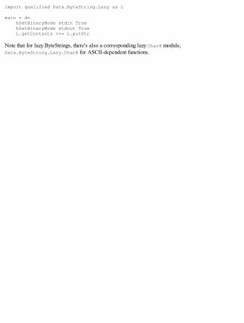
import qualified Data.ByteString.Lazy as L

main = do hSetBinaryMode stdin True hSetBinaryMode stdout True L.getContents >>= L.putStr

Note that for lazy ByteStrings, there's also a corresponding lazy Char8 module,Data.ByteString.Lazy.Char8 for ASCII-dependent functions.

Textual I/OAlthough String is a perfectly fine datatype to use in non-critical applications and for small strings,they're horribly space-inefficient for large strings and not completely Unicode-correct. The Text datatypes, strict and lazy, from the text package are a lot better datatypes for larger strings.

The IO functions for Texts are again named just like IO functions for Strings and ByteStrings, but forsome reason IO functions are in their own modules named Data.Text.IO and Data.Text.Lazy.IO.

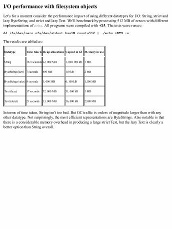
I/O performance with filesystem objectsLet's for a moment consider the performance impact of using different datatypes for I/O: String, strict andlazy ByteString, and strict and lazy Text. We'll benchmark by processing 512 MB of zeroes with differentimplementations of echo. All programs were compiled with -O3. The tests were run as:

dd if=/dev/zero of=/dev/stdout bs=1M count=512 | ./echo +RTS -s

The results are tabled as:

Datatype Time taken Heap allocations Copied in GC Memory in use

String 18.4 seconds 22, 000 MB 1, 000, 000 kB 1 MB

ByteString (lazy) 7 seconds 550 MB 110 kB 2 MB

ByteString (strict) 8 seconds 1, 000 MB 6, 100 kB 1,100 MB

Text (lazy) 17 seconds 32, 000 MB 31, 000 kB 1 MB

Text (strict) 21 seconds 33, 000 MB 56, 000 kB 2,900 MB

In terms of time taken, String isn't too bad. But GC traffic is orders of magnitude larger than with anyother datatype. Not surprisingly, the most efficient representations are ByteStrings. Also notable is thatthere is a considerable memory overhead in producing a large strict Text, but the lazy Text is clearly abetter option than String overall.

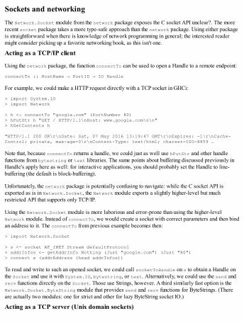
Sockets and networkingThe Network.Socket module from the network package exposes the C socket API unclear?. The morerecent socket package takes a more type-safe approach than the network package. Using either packageis straightforward when there is knowledge of network programming in general; the interested readermight consider picking up a favorite networking book, as this isn't one.

Acting as a TCP/IP client

Using the network package, the function connectTo can be used to open a Handle to a remote endpoint:

connectTo :: HostName → PortID → IO Handle

For example, we could make a HTTP request directly with a TCP socket in GHCi:

> import System.IO> import Network

> h <- connectTo "google.com" (PortNumber 80)> hPutStr h "GET / HTTP/1.1\nHost: www.google.com\n\n"> hGetContents h

"HTTP/1.1 200 OK\r\nDate: Sat, 07 May 2016 13:19:47 GMT\r\nExpires: -1\r\nCache-Control: private, max-age=0\r\nContent-Type: text/html; charset=ISO-8859 …

Note that, because connectTo returns a handle, we could just as well use hPutStr and other handlefunctions from bytestring or text libraries. The same points about buffering discussed previously inHandle's apply here as well: for interactive applications, you should probably set the Handle to line-buffering (the default is block-buffering).

Unfortunately, the network package is potentially confusing to navigate: while the C socket API isexported as is in Network.Socket, the Network module exports a slightly higher-level but muchrestricted API that supports only TCP/IP.

Using the Network.Socket module is more laborious and error-prone than using the higher-levelNetwork module. Instead of connectTo, we would create a socket with correct parameters and then bindan address to it. The connectTo from previous example becomes then:

> import Network.Socket

> s <- socket AF_INET Stream defaultProtocol> addrInfos <- getAddrInfo Nothing (Just "google.com") (Just "80")> connect s (addrAddress (head addrInfos))

To read and write to such an opened socket, we could call socketToHandle on s to obtain a Handle onthe Socket and use it with System.IO, bytestring, or text. Alternatively, we could use the send andrecv functions directly on the Socket. Those use Strings, however. A third similarly fast option is theNetwork.Socket.ByteString module that provides send and recv functions for ByteStrings. (Thereare actually two modules: one for strict and other for lazy ByteString socket IO.)

Acting as a TCP server (Unix domain sockets)

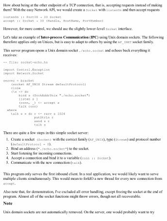
How about being at the other endpoint of a TCP connection, that is, accepting requests instead of makingthem? With the easy Network API, we would create a Socket with listenOn and then accept requests

listenOn :: PortID → IO Socketaccept :: Socket → IO (Handle, HostName, PortNumber)

However, for more control, we should use the slightly lower-level Socket interface.

Let's take an example of Inter-process Communication (IPC) using Unix domain sockets. The followingtherefore applies only on Unices, but is easy to adapt to others by using the AF_INET socket family.

This server program opens a Unix domain socket ./echo.socket and echoes back everything itreceives:

-- file: socket-echo.hs

import Control.Exceptionimport Network.Socket

server = bracket (socket AF_UNIX Stream defaultProtocol) close (\s -> do bind s (SockAddrUnix "./echo.socket") listen s 1 (conn, _) <- accept s talk conn) where talk s = do r <- recv s 1024 putStrLn r send s r talk s

There are quite a few steps in this simple socket server:

1. Create a socket (Socket) with the correct family (AF_UNIX), type (Stream) and protocol number(defaultProtocol = 0).

2. Bind an address ("./echo.socket") to the socket.3. Start listening for incoming connections.4. Accept a connection and bind it to a variable (conn :: Socket).5. Communicate with the new connection (talk).

This program only serves the first inbound client. In a real application, we would likely want to servemultiple clients simultaneously. This would mean to forkIO a new thread for every new connection fromaccept.

Also note that, for demonstration, I've excluded all error handling, except freeing the socket at the end ofprogram. Almost all of the socket functions might throw errors, though not all recoverable.

Note

Unix domain sockets are not automatically removed. On the server, one would probably want to try

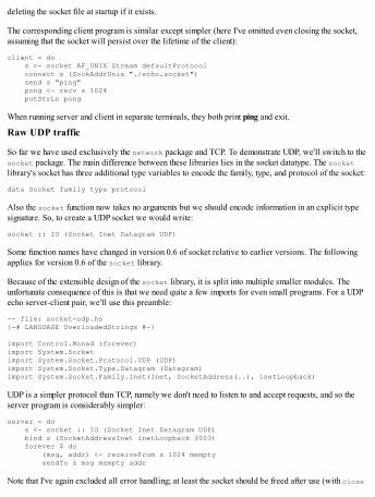
deleting the socket file at startup if it exists.

The corresponding client program is similar except simpler (here I've omitted even closing the socket,assuming that the socket will persist over the lifetime of the client):

client = do s <- socket AF_UNIX Stream defaultProtocol connect s (SockAddrUnix "./echo.socket") send s "ping" pong <- recv s 1024 putStrLn pong

When running server and client in separate terminals, they both print ping and exit.

Raw UDP traffic

So far we have used exclusively the network package and TCP. To demonstrate UDP, we'll switch to thesocket package. The main difference between these libraries lies in the socket datatype. The socketlibrary's socket has three additional type variables to encode the family, type, and protocol of the socket:

data Socket family type protocol

Also the socket function now takes no arguments but we should encode information in an explicit typesignature. So, to create a UDP socket we would write:

socket :: IO (Socket Inet Datagram UDP)

Some function names have changed in version 0.6 of socket relative to earlier versions. The followingapplies for version 0.6 of the socket library.

Because of the extensible design of the socket library, it is split into multiple smaller modules. Theunfortunate consequence of this is that we need quite a few imports for even small programs. For a UDPecho server-client pair, we'll use this preamble:

-- file: socket-udp.hs{-# LANGUAGE OverloadedStrings #-}

import Control.Monad (forever)import System.Socketimport System.Socket.Protocol.UDP (UDP)import System.Socket.Type.Datagram (Datagram)import System.Socket.Family.Inet(Inet, SocketAddress(..), inetLoopback)

UDP is a simpler protocol than TCP, namely we don't need to listen to and accept requests, and so theserver program is considerably simpler:

server = do s <- socket :: IO (Socket Inet Datagram UDP) bind s (SocketAddressInet inetLoopback 3003) forever $ do (msg, addr) <- receiveFrom s 1024 mempty sendTo s msg mempty addr

Note that I've again excluded all error handling; at least the socket should be freed after use (with close

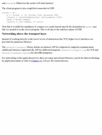
and bracket). Otherwise the socket will leak memory!

The client program is also simplified somewhat in UDP:

client = do s <- socket :: IO (Socket Inet Datagram UDP) connect s (SocketAddressInet inetLoopback 3003) send s "ping" mempty receive s 1024 mempty >>= print

Note that it wouldn't be mandatory to connect; we could instead specify the destination in sendTo justlike we needed to in the server program. This is all due to the stateless nature of UDP.

Networking above the transport layer

Instead of working directly in the lower levels of abstraction like TCP, higher-level interfaces areprovided by numerous libraries.

The network-transport library defines an abstract API for endpoint-to-endpoint communication.Additional libraries implement the API for different transports: network-transport-tcp for TCP andnetwork-transport-zeromq for ZeroMQ transports.

For networking in the application level, there are many specialized libraries; search for them in Hackageby application name or refer to Chapter 14, Library Recommendations.

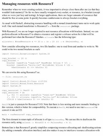
Managing resources with ResourceTRemember when we were creating sockets, it was important to always close them after use (so that theywouldn't leak memory)? So far we have usually wrapped every socket, or resource, in a bracket (exceptwhen we were just lazy and testing). In larger applications, there are larger amounts of resources thatshould be free at some point. It quickly becomes cumbersome to always bracket everything.

As usual with Haskell, abstracting resource handling with a monad (transformer) turns out to work quitewell. One such monad transformer is ResourceT m a from the resourcet package.

With ResourceT, we are no longer required to nest resource allocations with brackets. Instead, we canperform allocate in ResourceT to obtain a resource and register a release action for it that will beperformed last when the ResourceT finishes. allocate has the following type:

allocate:: MonadResource m => IO a → (a → IO ()) → m (ReleaseKey, a)

Now consider allocating two resources, two file handles: one to read from and another to write to. Wecould write two nested brackets as such:

import Control.Exceptionimport System.IO

copy_bracket :: IO ()copy_bracket = bracket (openFile "read.txt" ReadMode) hClose $ \f1 → bracket (openFile "write.txt" WriteMode) hClose $ \f2 → hGetContents f1 >>= hPutStr f2

We can rewrite this using ResourceT as:

-- file: resourcet.hs

import Control.Monad.IO.Class (liftIO)import Control.Monad.Trans.Resourceimport System.IO

copy_resourcet :: ResIO ()copy_resourcet = do (_, f1) <- allocate (openFile "read.txt" ReadMode) hClose (_, f2) <- allocate (openFile "write.txt" WriteMode) hClose liftIO $ hGetContents f1 >>= hPutStr f2

ResIO is just a synonym for ResourceT I/O. Note that there is less nesting and more monadic binding inthis version, which is better for composability. To execute a ResIO, we need to use run ResourceT toconvert it into an I/O:

main = runResourceT copy_resourcet

The first element in return tuple of allocate is of type ReleaseKey. We can use this to deallocate theresource early, using release :: MonadIO m => ReleaseKey → m ().

Bottom line is that ResourceT greatly simplifies composing resource-allocating and -deallocating actions(by adding a monadic allocation interface) and also makes it easy to interleave resource allocation with

effects from other monads (by being a transformer).

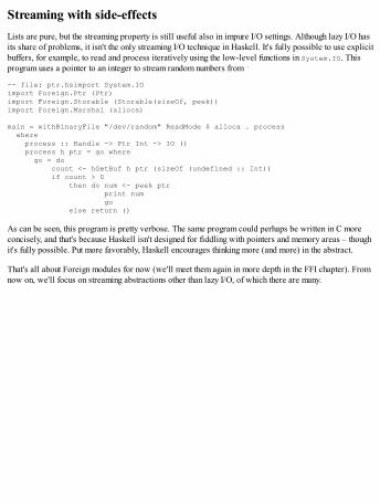
Streaming with side-effectsLists are pure, but the streaming property is still useful also in impure I/O settings. Although lazy I/O hasits share of problems, it isn't the only streaming I/O technique in Haskell. It's fully possible to use explicitbuffers, for example, to read and process iteratively using the low-level functions in System.IO. Thisprogram uses a pointer to an integer to stream random numbers from `

-- file: ptr.hsimport System.IOimport Foreign.Ptr (Ptr)import Foreign.Storable (Storable(sizeOf, peek))import Foreign.Marshal (alloca)

main = withBinaryFile "/dev/random" ReadMode $ alloca . process where process :: Handle -> Ptr Int -> IO () process h ptr = go where go = do count <- hGetBuf h ptr (sizeOf (undefined :: Int)) if count > 0 then do num <- peek ptr print num go else return ()

As can be seen, this program is pretty verbose. The same program could perhaps be written in C moreconcisely, and that's because Haskell isn't designed for fiddling with pointers and memory areas – thoughit's fully possible. Put more favorably, Haskell encourages thinking more (and more) in the abstract.

That's all about Foreign modules for now (we'll meet them again in more depth in the FFI chapter). Fromnow on, we'll focus on streaming abstractions other than lazy I/O, of which there are many.

Choosing a streaming libraryStreaming frameworks in Haskell have come a long way along the years, starting with lazy I/O. Theproblem with lazy I/O is foremost unpredictable resource handling, and that there is little control overwhen given effects happen precisely, because effects are interleaved with pure code. This allows forelegant code in small scale, but it becomes hard to control effects in larger scale.

In the 00s, work by Oleg Kiselyov initiated a surge of streaming libraries. Some of the first onespublished on Hackage were iteratee, enumerator, and iterIO at the turn of 2010. Instead ofimperatively using buffers for streaming data, iteratee-based I/O abstracts such patterns in composablemonadic actions. Unlike lazy I/O, iteratee based I/O is strict (in I/O, at least).

Nowadays, the libraries most seen in use with new code include pipes, conduit, and io-streams.pipes and conduit evolved simultaneously and hence they have a lot of overlap in their feature sets.Later versions of conduit actually featured a heavy internal redesign largely influenced by pipes. Forthose interested in such things, it's worth mentioning that the types and most functions in pipes have beenchecked using Coq (a theorem proving system) to ensure that the implementation is a law-abidingcategory.

An unfortunate feature of both conduit and pipes is their type framework: the types are hard to wrapone's head around even for a seasoned Haskeller. On the other hand, io-streams library has its focus onuser-friendliness with its simple types (and is restricted to I/O).

Both pipes and conduits are very flexible, but if you're really sure you need even more control andmore abstractions over your streams in the form of networked stream transducers, perhaps you shouldtake a look at the machines library by Edward Kmett.

In this section, we'll first introduce io-streams and then pipes and conduits.

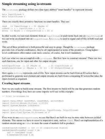
Simple streaming using io-streamsThe io-streams package defines two data types dubbed "smart handles" to represent streams:

data InputStream cdata OutputStream c

There are exactly three primitive functions on smart handles. They are:

read :: InputStream c → IO (Maybe c)unRead :: c → InputStream c → IO ()write :: Maybe c → OutputStream c → IO ()

In other words, we can read elements from an InputStream or push items back into an InputStream; orwe can write an element into an OutputStream. A Nothing is used to signal end-of-file in both read andwrite.

This set of three primitives is both powerful and easy to grasp. Though the io-streams packageprovides lots of useful combinators, they're all implemented in terms of the primitives. Using higher-level combinators often makes code more concise, of course, but it isn't mandatory.

Let's see what we can accomplish with io-streams. But first: how to construct streams? There are twosuch functions, one for input and other for output streams:

makeInputStream :: IO (Maybe a) → IO (InputStream a)makeOutputStream :: (Maybe a → IO ()) → IO (OutputStream a)

Here again, Nothing represents end-of-file. New input streams can be built from an IO action that isperformed to generate next element and output streams are built from a consuming IO action that takes theinput element as argument.

Creating input streams

Now we are ready to build some streams. The first stream we build will be one that generates randomnumbers. First things first, here are some imports we'll use in this example:

-- file: io-streams.hs

import Data.IORef (newIORef, readIORef, writeIORef)import Control.Monad.IO.Class (liftIO)import System.Random (randomIO)

import System.IO.Streams (Generator, InputStream, OutputStream)import qualified System.IO.Streams as S

If we were to use makeInputStream, we see that there's no built-in way to store state between yieldedelements. This means we have to resort to imperative state, such as IORef. Here's an implementation of arandom stream using an IORef to store the count of numbers left to produce:

randomInputStreamRef :: Int -> IO (InputStream Double)randomInputStreamRef count = do ref <- newIORef count S.makeInputStream $ do

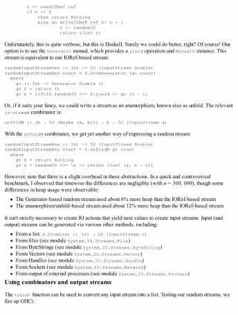
n <- readIORef ref if n <= 0 then return Nothing else do writeIORef ref $! n - 1 r <- randomIO return (Just r)

Unfortunately, this is quite verbose, but this is Haskell. Surely we could do better, right? Of course! Oneoption is to use the Generator monad, which provides a yield operation and MonadIO instance. Thisstream is equivalent to our IORef-based stream:

randomInputStreamGen :: Int -> IO (InputStream Double)randomInputStreamGen count = S.fromGenerator (go count) where go :: Int -> Generator Double () go 0 = return () go n = liftIO randomIO >>= S.yield >> go (n – 1)

Or, if it suits your fancy, we could write a stream as an anamorphism, known also as unfold. The relevantio-stream combinator is:

unfoldM :: (b → IO (Maybe (a, b))) → b → IO (InputStream a)

With the unfoldM combinator, we get yet another way of expressing a random stream:

randomInputStreamAna :: Int -> IO (InputStream Double)randomInputStreamAna count = S.unfoldM go count where go 0 = return Nothing go n = randomIO >>= \r -> return (Just (r, n – 1))

However, note that there is a slight overhead in these abstractions. In a quick and controversialbenchmark, I observed that timewise the differences are negligible (with n = 500, 000), though somedifferences in heap usage were observable:

The Generator-based random stream used about 6% more heap than the IORef-based streamThe anamorphism/unfold-based stream used about 12% more heap than the IORef-based stream

It isn't strictly necessary to create IO actions that yield next values to create input streams. Input (andoutput) streams can be generated via various other methods, including:

From a list: S.fromList :: [c] → IO (InputStream c)From files (see module System.IO.Streams.File)From ByteStrings (see module System.IO.Streams.ByteString)From Vectors (see module System.IO.Streams.Vector)From Handles (see module System.IO.Streams.Handle)From Sockets (see module System.IO.Streams.Network)From output of external processes (see module System.IO.Streams.Process)

Using combinators and output streams

The toList function can be used to convert any input stream into a list. Testing our random streams, wefire up GHCi:

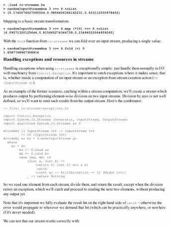
> :load io-streams.hs> randomInputStreamAna 3 >>= S.toList> [0.1745076027065504,0.9856406364162231,0.653112050978402]

Mapping is a basic stream transformation:

> randomInputStreamAna 3 >>= S.map (*10) >>= S.toList[6.09571320125644,5.815660274344739,0.23496022064959265]

With the fold function from io-streams we can fold over an input stream, producing a single value:

> randomInputStreamAna 3 >>= S.fold (+) 01.6587768967308916

Handling exceptions and resources in streams

Handling exceptions when using io-streams is exceptionally simple: just handle them normally in I/Owith machinery from Control.Exception. It's important to catch exceptions where it makes sense, thatis, whether inside a computation of an input stream or an exception from stream creation action (IO(InputStream a)).

As an example of the former scenario, catching within a stream computation, we'll create a stream whichproduces output by performing element-wise division on two input streams. Division by zero is not welldefined, so we'll want to omit such results from the output stream. Here's the combinator:

-- file: io-streams-exceptions.hs

import Control.Exceptionimport System.IO.Streams (Generator, InputStream, OutputStream)import qualified System.IO.Streams as S

divideBy :: InputStream Int -> InputStream Int -> IO (InputStream Int)divideBy as bs = S.makeInputStream go where go = do ma <- S.read as mb <- S.read bs case (ma, mb) of (Just a, Just b) -> (return $! Just $! div a b) `catch` (const go :: ArithException -> IO (Maybe Int)) _ -> return Nothing

So we read one element from each stream, divide them, and return the result, except when the divisionraises an exception, which we'll catch and proceed to reading the next two elements, without producingany output yet.

Note that it's important we fully evaluate the result Int on the right-hand side of catch – otherwise theerror would propagate to wherever we demand that Int (which can be practically anywhere, or nowhereif it's never needed).

We can test that our stream works correctly with:

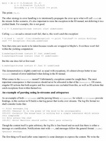
main = do x <- S.fromList [0..4] y <- S.fromList [1,0,0,2] divideBy x y >>= S.toList >>= print

This prints [0,1].

The other strategy to error handling is to intentionally propagate the error up to what will call read onthe stream. In this scenario, it's also important to raise the exception in the IO monad, not deferring it in ayielded thunk. For example, this is not good:

> s <- S.makeInputStream (return (Just undefined))

Calling read on such a stream won't fail, that is, this won't catch the exception:

> S.read s `catch` (\(e::SomeException) -> print "catched" >> return Nothing)Just *** Exception: Prelude.undefined

Note that extra care needs to be taken because results are wrapped in Maybe's. Even these won't failwithin the yielding computation:

S.makeInputStream (return $! Just undefined)S.makeInputStream (return (Just $! undefined))

But this one does fail at first read:

S.makeInputStream (return $! Just $! undefined)

This demonstration is slightly contrived: as usual with exceptions, it's almost always better to usethrowIO instead of error/undefined when failing in the IO monad.

What comes to the Generator monad? Unfortunately, exceptions cannot be caught there. The mostimportant consequence is that resources should never be allocated in that of the Generator. Of course,singular IO actions that both acquire and free resources are excluded from this, as well as IO actions thatcatch exceptions from within themselves.

An example of parsing using io-streams and attoparsec

As an example of both io-streams and the parsing library attoparsec for which io-streams providebindings, in this section we'll build a chat log parser that works over streams. The log file format weshall consider looks like:

-- file: messages.log[00:50] <Seneca> It is the power of the mind to be unconquerable[05:03] <Leibniz> The monad here is nothing but a simple substance which enters into compounds=== Erin enters the chat[00:01] <Erin> Warriors should suffer their pain silently

Though the content itself is quite arbitrary, the log file is line-based and on each line there is either amessage or a notification. Notifications start with ===, and messages follow the general format: [time]<person> message.

The first thing we'll need (after some imports) is some datatypes to express the content. We write the

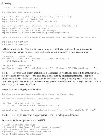
following:

-- file: io-streams-parser.hs

{-# LANGUAGE OverloadedStrings #-}

import Data.Monoid ((<>))import Control.Applicative ((<|>))import Data.ByteString (ByteString)import Data.Attoparsec.ByteString.Char8 as PC8

import System.IO.Streams (Generator, InputStream, OutputStream)import qualified System.IO.Streams as Simport System.IO.Streams.File (withFileAsInput)import System.IO.Streams.Attoparsec (parserToInputStream)

data Line = Notification ByteString| Message Time User ByteString deriving Show

type Time = ByteStringtype User = ByteString

Self-explanatory so far! Now for the parser, or parsers. We'll start with simple ones: parsers fortimestamps and persons or users. Using applicative syntax, we can write these concisely as:

timeParser :: Parser TimetimeParser = char '[' *> takeWhile1 (/= ']') <* char ']' <* PC8.takeWhile (== ' ')

userParser :: Parser UseruserParser = char '<' *> takeWhile1 (/= '>') <* char '>'<* PC8.takeWhile (== ' ')

The (p *> q) combinator simply applies parser p, discards its results, and proceeds to apply parser q.The (<*) combinator is like (*>) but takes results only from the first argument instead. The parserprimitives char and takeWhile come from the attoparsec library. Both (*>) and (<*) are infixl,meaning they associate to the left and so the whole parser can be read from left to right. The final result iswhere a (*>) is followed by a (<*).

Parser for a line is slightly more involved:

lineParser, messageParser, notificationParser :: Parser Line

lineParser = messageParser <|> notificationParser

notificationParser = string "=== " *> (Notification <$> PC8.takeWhile (/= '\n'))

messageParser = Message <$> timeParser<*> userParser<*> PC8.takeWhile (/= '\n')

The (p <|> q) combinator tries to apply parser p, and if it fails, proceeds with q.

We can verify that our parsers work, in GHCi:

> :load io-streams-parser.hs> > parseOnly lineParser "[time] <user> a message"Right (Message "time" "user" "a message")> parseOnly lineParser "=== notification"Right (Notification "notification")

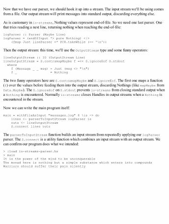
Now that we have our parser, we should hook it up into a stream. The input stream we'll be using comesfrom a file. Our output stream will print messages into standard output, discarding everything else.

As is customary in io-streams, Nothing values represent end-of-file. So we need one last parser. Onethat tries reading a next line, returning nothing when reaching the end-of-file:

logParser :: Parser (Maybe Line)logParser = (endOfInput *> pure Nothing) <|> (fmap Just lineParser <* PC8.takeWhile (== '\n'))

Then the output stream: this time, we'll use the OutputStream type and some funny operators:

lineOutputStream :: IO (OutputStream Line)lineOutputStream = S.contramapMaybe f =<< S.ignoreEof S.stdout where f (Message _ _ msg) = Just (msg <> "\n") f _ = Nothing

The two funny operators here are S.contramapMaybe and S.ignoreEof. The first one maps a function(f) over the values before feeding them into the output stream, discarding Nothings (like mapMaybe fromData.Maybe). The S.ignoreEof on S.stdout prevents io-streams from closing standard output whena Nothing is encountered. Normally io-streams closes Handles in output streams when a Nothing isencountered in the stream.

Now we can write the main program itself:

main = withFileAsInput "messages.log" $ \is -> do lines <- parserToInputStream logParser is outs <- lineOutputStream S.connect lines outs

The parserToInputStream function builds an input stream from repeatedly applying our logParserparser. The S.connect is a utility function which combines an input stream with an output stream. Wecan confirm our program does what we intended:

> :load io-streams-parser.hs> mainIt is the power of the mind to be unconquerableThe monad here is nothing but a simple substance which enters into compoundsWarriors should suffer their pain silently

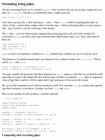
Streaming using pipesThe next streaming library we'll consider is pipes. Now we have only one stream type compared to twotypes in io-streams, but that is a considerably more complicated type:

data Proxy a' a b' b m r

Now skim your eyes for a while and unsee a' and b'. Then Proxy would be something that takes invalues of type a and produces output values of another type b while performing effects in some monad m.The r type variable is just the result type of the monad.

The a' and b' exist for bidirectional communication along pipelines and aren't often needed. Forconvenience, pipes provides some type synonyms that simplify pipes types a lot. Three most used ofthose are:

type Producer' b m rtype Consumer' a m rtype Pipe a b m r

Type variables correspond to variables in Proxy. Omitted type variables are not relevant here now.

The primitives in (unidirectional) pipes are reduced to two, contrary to three, for io-streams. They'recalled await and yield:

await :: Monad m => Consumer' a m ayield :: Monad m => b -> Producer' b m ()

The types actually tell precisely what these functions do. await returns a value that was yielded from theinput-side of a pipe in the monad (the first and last type variables are unified). yield takes as argument avalue of type that is unified with the output-side's type and passes it forward in the stream.

We can say that consumers await whereas producers yield. Now note that Pipe is a strictly more generaltype than consumers or producers. So pipes can both yield and await.

Here is one example of each, producer, consumer and pipe:

-- file: pipes.hs

import Control.Monadimport System.Random (randomIO)import Pipes

randoms :: Producer' Int IO ()randoms = forever (liftIO randomIO >>= yield)

taking :: Monad m => Int -> Pipe a a m ()taking 0 = return ()taking n = await >>= yield >> taking (n - 1)

printing :: Show a => Consumer' a IO ()printing = forever (await >>= liftIO . print)

Composing and executing pipes

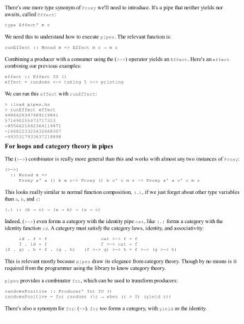
There's one more type synonym of Proxy we'll need to introduce. It's a pipe that neither yields norawaits, called Effect:

type Effect' m r

We need this to understand how to execute pipes. The relevant function is:

runEffect :: Monad m => Effect m r → m r

Combining a producer with a consumer using the (>->) operator yields an Effect. Here's an effectcombining our previous examples:

effect :: Effect IO ()effect = randoms >-> taking 5 >-> printing

We can run this effect with runEffect:

> :load pipes.hs> runEffect effect4486626397489119841571690255473717323-8556621642364119471-1668223325432668307-4935317933637218898

For loops and category theory in pipes

The (>->) combinator is really more general than this and works with almost any two instances of Proxy:

(>->) :: Monad m => Proxy a' a () b m r-> Proxy () b c' c m r -> Proxy a' a c' c m r

This looks really similar to normal function composition, (.), if we just forget about other type variablesthan a, b, and c:

(.) :: (b → c) → (a → b) → (a → c)

Indeed, (>->) even forms a category with the identity pipe cat, like (.) forms a category with theidentity function id. A category must satisfy the category laws, identity, and associativity:

id . f = f cat >-> f = f f . id = f f >-> cat = f(f . g) . h = f . (g . h) (f >-> g) >-> h = f >-> (g >-> h)

This is relevant mostly because pipes draw its elegance from category theory. Though by no means is itrequired from the programmer using the library to know category theory.

pipes provides a combinator for, which can be used to transform producers:

randomsPositive :: Producer' Int IO ()randomsPositive = for randoms (\r → when (r > 0) (yield r))

There's also a synonym for for: (~>). for too forms a category, with yield as the identity.

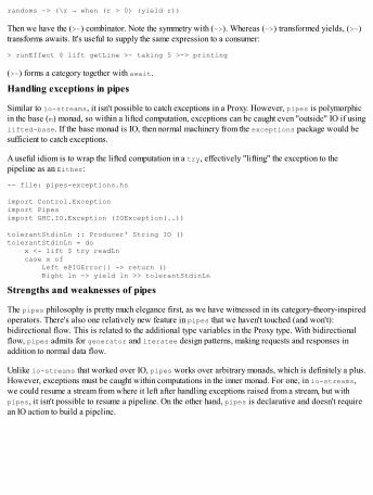
randoms ~> (\r → when (r > 0) (yield r))

Then we have the (>~) combinator. Note the symmetry with (~>). Whereas (~>) transformed yields, (>~)transforms awaits. It's useful to supply the same expression to a consumer:

> runEffect $ lift getLine >~ taking 5 >-> printing

(>~) forms a category together with await.

Handling exceptions in pipes

Similar to io-streams, it isn't possible to catch exceptions in a Proxy. However, pipes is polymorphicin the base (m) monad, so within a lifted computation, exceptions can be caught even "outside" IO if usinglifted-base. If the base monad is IO, then normal machinery from the exceptions package would besufficient to catch exceptions.

A useful idiom is to wrap the lifted computation in a try, effectively "lifting" the exception to thepipeline as an Either:

-- file: pipes-exceptions.hs

import Control.Exceptionimport Pipesimport GHC.IO.Exception (IOException(..))

tolerantStdinLn :: Producer' String IO ()tolerantStdinLn = do x <- lift $ try readLn case x of Left e@IOError{} -> return () Right ln -> yield ln >> tolerantStdinLn

Strengths and weaknesses of pipes

The pipes philosophy is pretty much elegance first, as we have witnessed in its category-theory-inspiredoperators. There's also one relatively new feature in pipes that we haven't touched (and won't):bidirectional flow. This is related to the additional type variables in the Proxy type. With bidirectionalflow, pipes admits for generator and iteratee design patterns, making requests and responses inaddition to normal data flow.

Unlike io-streams that worked over IO, pipes works over arbitrary monads, which is definitely a plus.However, exceptions must be caught within computations in the inner monad. For one, in io-streams,we could resume a stream from where it left after handling exceptions raised from a stream, but withpipes, it isn't possible to resume a pipeline. On the other hand, pipes is declarative and doesn't requirean IO action to build a pipeline.

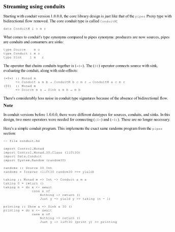
Streaming using conduitsStarting with conduit version 1.0.0.0, the core library design is just like that of the pipes Proxy type withbidirectional flow removed. The core conduit type is called ConduitM:

data ConduitM i o m r

What comes to conduit's type synonyms compared to pipes synonyms: producers are now sources, pipesare conduits and consumers are sinks:

type Source m otype Conduit i m otype Sink i m r

The operator that chains conduits together is (=$=). The ($$) operator connects source with sink,evaluating the conduit, along with side-effects:

(=$=) :: Monad m => Conduit a m b → ConduitM b c m r → ConduitM a c m r($$) :: Monad m => Source m a → Sink a m b → m b

There's considerably less noise in conduit type signatures because of the absence of bidirectional flow.

Note

In conduit versions before 1.0.0.0, there were different datatypes for sources, conduits, and sinks. In thisdesign, two more operators were needed for connecting (($=) and (=$)). These are no longer necessary.

Here's a simple conduit program. This implements the exact same randoms program from the pipessection:

-- file conduit.hs

import Control.Monadimport Control.Monad.IO.Class (liftIO)import Data.Conduitimport System.Random (randomIO)

randoms :: Source IO Intrandoms = forever (liftIO randomIO >>= yield)

taking :: Monad m => Int -> Conduit a m ataking 0 = return ()taking n = do x <- await case x of Nothing -> return () Just y -> yield y >> taking (n - 1)

printing :: Show a => Sink a IO ()printing = do x <- await case x of Nothing -> return () Just y -> liftIO (print y) >> printing

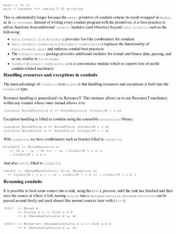
main :: IO ()main = randoms =$= taking 5 $$ printing

This is substantially longer because the await primitive of conduits returns its result wrapped in Maybe,as in io-streams. Instead of writing every conduit program with the primitives, it is best practice toutilize functions from additional conduit modules (and libraries) beyond Data.Conduit, such as thefollowing:

Data.Conduit.List (conduit) provides list-like combinators for conduitsData.Conduit.Combinators (conduit-combinators) replaces the functionality ofData.Conduit.List and enforces conduit best practicesThe conduit-extra package provides additional modules for textual and binary data, parsing, andso on, similar to io-streamsConduit (conduit-combinators) is a convenience module which re-exports lots of usefulconduit-related machinery

Handling resources and exceptions in conduits

The main advantage of conduits over pipes is that handling resources and exceptions is built into theConduitM type.

Resource handling is generalized via ResourceT. This instance allows us to use ResourceT machinerywithin any conduit whose inner monad allows it to:

instance MonadResource m => MonadResource (ConduitM i o m)

Exception handling is lifted to conduits using the extensible extensions library:

instance MonadThrow m => MonadThrow (ConduitM i o m)instance MonadCatch m => MonadCatch (ConduitM i o m)

With conduits, we have combinators such as bracket lifted to conduits:

bracketP :: MonadResource m => IO a → (a → IO ()) → (a → ConduitM i o m r) → ConduitM i o m r

And also catch lifted to conduits:

catchC :: (MonadBaseControl IO m, Exception e) => ConduitM i o m r → (e → ConduitM i o m r) → ConduitM i o m r

Resuming conduits

It is possible to feed some source into a sink, using the ($$+), process, until the sink has finished and thensave the source at where it left, turning Source into a ResumableSource. ResumableSources can bepassed around freely and used almost like normal sources later with ($$++):

($$+) :: Monad m => Source m a -> Sink a m b -> m (ResumableSource m a, b)

($$++) :: Monad m=> ResumableSource m a -> Sink a m b -> m (ResumableSource m a, b)

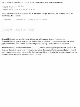
For an example, consider this Source which yields consecutive numbers from zero:

counter :: Source IO Intcounter = go 0 where go n = yield n >> go (n + 1)

With ResumableSources, we can use this as a source of unique identifiers, for example. Here's anillustrating GHCi session:

> (resume,_) <- counter $$+ taking 5 =$= printing01234> resume $$++ taking 3 =$= printing567

ResumableSources can also be converted into normal sources with unwrapResumable.ResumableSources give us back the nice feature that was built into io-streams and that was lost inpipes, namely first-class streams. But one thing is still missing which is related to exceptions.

When an exception was raised inside an io-stream stream, it would propagate upward, but leave thestream in the state it was at before raising the exception. To copy this behavior in conduits, we wouldcatch exceptions in conduit/sink and end computation. Then, as the pipeline stops accepting input, use($$+) to convert the source into an ResumableStream.

Logging in HaskellA final thing we'll consider is more related to I/O than streaming: logging in Haskell applications.Logging is important in any sufficiently important application.

In a small scale, a list- or DList-based WriterT monad is often all that is needed: it's simple andpotentially pure (if the underlying monad is pure). However, on a bigger scale it doesn't make sense tostore messages in an internal pure data structure. Instead, it's most efficient to write them to disk (or overa network) immediately (likely still using a buffer, though).

Furthermore, it would be nice if the logging functionality could be decoupled from other applicationcode, even reused between different applications.

A popular solution which provides just that kind of decoupling is the monad-logger library. It uses alibrary called Fastlogger, which provides logging that scales in multicore environments. Mostnotoriously, FastLogger is used in the Web Application Interface (WAI) package used by many high-performance Haskell web frameworks and applications.

Logging with FastLoggerThe core datatype in FastLogger is LoggerSet, whose constructors are not exposed. Internally, it holdsmultiple loggers, one for each OS thread (-N<x>). A LoggerSet is built with one of the smartconstructors:

newFileLoggerSet :: BufSize -> FilePath -> IO LoggerSetnewStdoutLoggerSet :: BufSize -> IO LoggerSetnewStderrLoggerSet :: BufSize -> IO LoggerSet

Log messages are written to that of a LoggerSet using pushLogStr(Ln):

pushLogStr :: LoggerSet → LogStr → IO ()

The LogStr datatype is also abstract (constructors not exposed). LogStr construction is overloaded viatype class ToLogStr, provided with default instances for textual data:

class ToLogStr msg where toLogStr :: msg → LogStr

instance ToLogStr Stringinstance ToLogStr ByteStringinstance ToLogStr Textinstance toLogStr LogStr

Here's a GHCi session to demonstrate usage:

> import System.Log.FastLogger> logger <- newStdoutLoggerSet defaultBufSize> pushLogStr logger (toLogStr "a log message")a log message

It's encouraged to create your own log message datatype and write custom instances for ToLogStr(inductively utilizing existing instances). For performance reasons, it's better to specialize your loggingfunctions to avoid ToLogStr dictionary-passing, as in pushLogStr.

Note that FastLogger provides the bare minimum needed for efficient logging: monomorphic file andstream loggers and a simple overloaded interface for building log messages. On top of this, it's easy tobuild other mechanisms, such as custom log messages and logging functions.

More abstract loggers

Version 2.4.4 of FastLogger had some new functionality. Among others, a new type alias wasintroduced: when we partially apply pushLogStr with a LoggerSet, we get the extremely simple yetpowerful FastLogger function:

type FastLogger = LogStr → IO ()

Now, instead of using LoggerSets directly, we can step up abstractions one notch. ThewithFastLogger function takes an argument of type LogType, with which we can build many kinds ofloggers:

withFastLogger :: LogType → IO (FastLogger → IO a) → IO a

This function takes care of closing the LoggerSet correctly, so you don't need to worry about leakingloggers. The second argument is a callback which can make use of the logger function. The differentconstructors of LogType initialize different kinds of loggers. In addition to stdout, stderr, and filelogging, it becomes trivial to create file-rotating loggers:

data LogType = LogNone | LogStdout BufSize | LogStderr BufSize | LogFileNoRotate FilePath BufSize | LogFile FileLogSpec BufSize | LogCallback FastLogger (IO ())

Timed log messagesIt's often very useful to have timestamps in log messages. However, in high-performance applicationswith high-frequency logging, date rendering becomes a bottleneck, unless we cache rendered dates.Fortunately, FastLogger (versions later than 2.4.4) comes with a solution for date caching that onlyrenders dates at most once per second. Timed FastLoggers have the type:

type TimedFastLogger = (FormattedTime → LogStr) → IO ()

Timed loggers are created with the withTimedFastLogger function:

withTimedFastLogger :: IO FormattedTime -> LogType -> (TimedFastLogger -> IO a) -> IO a

The first argument requires an IO action to return formatted time (ByteString), which we should buildwith newTimeCache:

newTimeCache :: TimeFormat -> IO (IO FormattedTime)

Just an IO action within an IO action. This is used as in:

> getTimeStamp <- newTimeCache "%Y-%m-%d %H:%M"> getTimeStamp"2016-05-11 15:02"

To attach timestamps into log messages, we need a log function which formats the timestamp. Here's onefor logging events of type String:

logFormat :: String -> FormattedTime -> LogStrlogFormat msg time = toLogStr time <> ": " <> toLogStr msg

Now let's put everything together into a complete program that logs something nonsensical (yet true).Let's try a top to bottom approach. We wish to write log messages with a simple IO action taking only ourlog message (String) as its argument. This is easily expressed as:

-- file: fastlogger.hs{-# LANGUAGE OverloadedStrings #-}

import Data.Monoidimport System.Log.FastLogger

type MyLogger = String -> IO ()

app :: MyLogger -> IO ()app log = do log "Haskell is fun" log "and logging is fun too!"

Now we only need the main that executes our application, supplying it with an appropriate logger. Thereis nothing new in the function body that follows – I have just combined everything we discussed so farabout (timed) logging and formatting:

main = do getTimeStamp <- newTimeCache "%Y-%m-%d %H:%M"

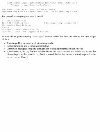
withTimedFastLogger getTimeStamp (LogStdout defaultBufSize) $ \logger -> app (logger . logFormat)

logFormat :: String -> FormattedTime -> LogStrlogFormat msg time = toLogStr time <> ": " <> toLogStr msg <> "\n"

Just to confirm everything works as it should:

> :load fastlogger.hs[1 of 1] Compiling Main ( fastlogger.hs, interpreted )Ok, modules loaded: Main.> main2016-05-11 16:20: Haskell is fun2016-05-11 16:20: and logging is fun too!

So what did we gain from using FastLogger? We wrote about four lines, but in those four lines we gotall these:

Timestamped log messages with a timestamp cache.Custom timestamp and log message formatting.Completely decoupled setup and configuration of logging from the application code.If you wanted to, the log function could be hidden in a Reader monad and write a log action, thuseliminating the need to pass the log function around. In fact, this pattern is already captured in themonad-logger library.

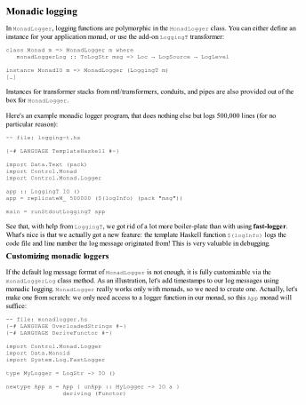
Monadic loggingIn MonadLogger, logging functions are polymorphic in the MonadLogger class. You can either define aninstance for your application monad, or use the add-on LoggingT transformer:

class Monad m => MonadLogger m where monadLoggerLog :: ToLogStr msg => Loc → LogSource → LogLevel

instance MonadIO m => MonadLogger (LoggingT m)[…]

Instances for transformer stacks from mtl/transformers, conduits, and pipes are also provided out of thebox for MonadLogger.

Here's an example monadic logger program, that does nothing else but logs 500,000 lines (for noparticular reason):

-- file: logging-t.hs

{-# LANGUAGE TemplateHaskell #-}

import Data.Text (pack)import Control.Monadimport Control.Monad.Logger

app :: LoggingT IO ()app = replicateM_ 500000 ($(logInfo) (pack "msg"))

main = runStdoutLoggingT app

See that, with help from LoggingT, we got rid of a lot more boiler-plate than with using fast-logger.What's nice is that we actually got a new feature: the template Haskell function $(logInfo) logs thecode file and line number the log message originated from! This is very valuable in debugging.

Customizing monadic loggers

If the default log message format of MonadLogger is not enough, it is fully customizable via themonadLoggerLog class method. As an illustration, let's add timestamps to our log messages usingmonadic logging. MonadLogger really works only with monads, so we need to create one. Actually, let'smake one from scratch: we only need access to a logger function in our monad, so this App monad willsuffice:

-- file: monadlogger.hs{-# LANGUAGE OverloadedStrings #-}{-# LANGUAGE DeriveFunctor #-}

import Control.Monad.Loggerimport Data.Monoidimport System.Log.FastLogger

type MyLogger = LogStr -> IO ()

newtype App a = App { unApp :: MyLogger -> IO a } deriving (Functor)

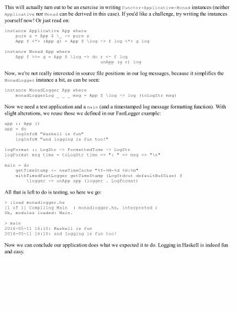
This will actually turn out to be an exercise in writing Functor-Applicative-Monad instances (neitherApplicative nor Monad can be derived in this case). If you'd like a challenge, try writing the instancesyourself now! Or just read on:

instance Applicative App where pure x = App $ \_ -> pure x App f <*> (App g) = App $ \log -> f log <*> g log

instance Monad App where App f >>= g = App $ \log -> do r <- f log unApp (g r) log

Now, we're not really interested in source file positions in our log messages, because it simplifies theMonadLogger instance a bit, as can be seen:

instance MonadLogger App where monadLoggerLog _ _ _ msg = App $ \log -> log (toLogStr msg)

Now we need a test application and a main (and a timestamped log message formatting function). Withslight alterations, we reuse those we defined in our FastLogger example:

app :: App ()app = do logInfoN "Haskell is fun" logInfoN "and logging is fun too!"

logFormat :: LogStr -> FormattedTime -> LogStrlogFormat msg time = toLogStr time <> ": " <> msg <> "\n"

main = do getTimeStamp <- newTimeCache "%Y-%M-%d %H:%m" withTimedFastLogger getTimeStamp (LogStdout defaultBufSize) $ \logger -> unApp app (logger . LogFormat)

All that is left to do is testing, so here we go:

> :load monadlogger.hs[1 of 1] Compiling Main ( monadlogger.hs, interpreted )Ok, modules loaded: Main.

> main2016-05-11 16:10: Haskell is fun2016-05-11 16:10: and logging is fun too!

Now we can conclude our application does what we expected it to do. Logging in Haskell is indeed funand easy.

SummaryIn this chapter we have covered the advantages and disadvantages of lazy I/O and its alternatives: strictI/O and some streaming solutions. We learned to connect to remote network endpoints as clients and towrite own network servers in Haskell. We also learned that acquired I/O resources such as handles andsockets must always be freed. For this, we considered two main solutions: functions such as bracketand the ResourceT monad transformer.

After reading this chapter you should now understand and be able to use lazy I/O without surprisingmemory leaks and correctly release all acquired resources as well as exceptions. You know and can usethree streaming libraries: rudimentary io-streams, elegant pipes, and industrial conduits. You arealso bound to enjoy doing logging from your Haskell programs with FastLogger and monads with monad-logger.

In the next chapter, we will focus on concurrent programming in Haskell. Light-Lightweight GHC threadsgive a lot of flexibility for the concurrent programmer, and software transactional memory provides aneasy-to-use framework for handling critical sections in a more abstract fashion.

Chapter 7. Concurrency and PerformanceWriting concurrent programs that are correct is hard: subtle race conditions, resources blocked byanother thread, asynchronous exceptions, and so on. Basically, a lot can go wrong. Remember that,whereas parallelism points to execution model (multiple threads running simultaneously), concurrency ismore like a paradigm: multiple threads working together, intertwined. However, concurrent threads areoften run in parallel for responsiveness and performance reasons.

In this chapter, we will write concurrent Haskell programs making use of light-weight threads and type-safe concurrency primitives like MVars. For complex programs, we will learn to build atomictransactions with Software Transactional Memory (STM).

We will consider some models for concurrent programming: asynchronous workers and actors. Andalthough asynchronous exceptions are usually to be avoided (like those from calls to error/undefined),asynchronous exceptions are useful for notifying one thread from another. Finally, we'll look at workingwith lifted concurrency operations to other monads besides IO, which can be extremely convenientsometimes.

We will cover:

Becoming familiar with light-weight threads, primitive concurrency functions, and mutablevariablesBuilding complex atomic transactions using Software Transactional MemoryUsing the Async API for concise asynchronous processingLifting concurrency operations and exception handling using MonadBase and MonadBaseControl

Threads and concurrency primitivesOne of the basic forms of concurrent programming involves sharing read-write data between threads.Usually data is shared via references. From fastest to most flexible, the three types of mutable referencesin Haskell are IORef, MVar, and STM. All three can be used, at least to some extent, in a thread-safemanner. We start our concurrent journey with a simple reference, IORef, and work our way to arbitrarilycomplex transactions using STM.

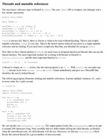
Threads and mutable referencesThe most basic reference type in Haskell is IORef. The core IORef API is compact, one datatype and afew atomic operations:

module Data.IORef

data IORef a

newIORef :: a → IO (IORef a)readIORef :: IORef a → IO awriteIORef :: IORef a → a → IO ()modifyIORef :: IORef a → (a → a) → IO ()atomicModifyIORef :: IORef a → (a → (a, b)) → IO b

IORef is always full, that is, there is always a value to be read without blocking. They're just simplemutable references. IORef is very fast. They're the fastest option when all you need is a single mutablereference and no locking. If you need more complexity than that, you shouldn't be using an IORef.

Now that we have shared memory (IORef), we need ways to program interleaved threads that can use theshared memory. The most important module for working with threads in Haskell isControl.Concurrent, and the most important function is forkIO:

forkIO :: IO () → IO ThreadId

A thread is simply an IO () action, like the main program is an IO (). With forkIO, we can make anyIO () execute in its own thread. Calls to forkIO return immediately and give us a ThreadID thatidentifies the newly forked thread.

The following program illustrates forking and mutable references. It prints multiple instances of a and bin some order for a split second:

-- ioref.hs

import Data.IORefimport Control.Concurrent

fun ref c = do x <- readIORef ref writeIORef ref c putStr x fun ref c

main = do ref <- newIORef "a" forkIO $ fun ref "a" forkIO $ fun ref "b" threadDelay 5000

We can run this via runhaskell ioref.hs. The output pattern looks like aabababababa and so on andis around 200 characters long. Note carefully that we didn't bother killing the child threads; in Haskell,when the main thread exits, all child threads will die too. However, we did use threadDelay, whichblocks the current thread for a given number of microseconds.

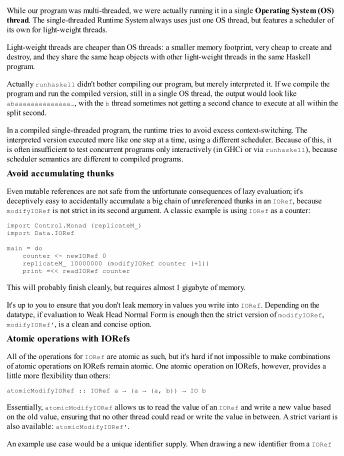
While our program was multi-threaded, we were actually running it in a single Operating System (OS)thread. The single-threaded Runtime System always uses just one OS thread, but features a scheduler ofits own for light-weight threads.

Light-weight threads are cheaper than OS threads: a smaller memory footprint, very cheap to create anddestroy, and they share the same heap objects with other light-weight threads in the same Haskellprogram.

Actually runhaskell didn't bother compiling our program, but merely interpreted it. If we compile theprogram and run the compiled version, still in a single OS thread, the output would look likeabaaaaaaaaaaaaaa…, with the b thread sometimes not getting a second chance to execute at all within thesplit second.

In a compiled single-threaded program, the runtime tries to avoid excess context-switching. Theinterpreted version executed more like one step at a time, using a different scheduler. Because of this, itis often insufficient to test concurrent programs only interactively (in GHCi or via runhaskell), becausescheduler semantics are different to compiled programs.

Avoid accumulating thunks

Even mutable references are not safe from the unfortunate consequences of lazy evaluation; it'sdeceptively easy to accidentally accumulate a big chain of unreferenced thunks in an IORef, becausemodifyIORef is not strict in its second argument. A classic example is using IORef as a counter:

import Control.Monad (replicateM_)import Data.IORef

main = do counter <- newIORef 0 replicateM_ 10000000 (modifyIORef counter (+1)) print =<< readIORef counter

This will probably finish cleanly, but requires almost 1 gigabyte of memory.

It's up to you to ensure that you don't leak memory in values you write into IORef. Depending on thedatatype, if evaluation to Weak Head Normal Form is enough then the strict version of modifyIORef,modifyIORef', is a clean and concise option.

Atomic operations with IORefs

All of the operations for IORef are atomic as such, but it's hard if not impossible to make combinationsof atomic operations on IORefs remain atomic. One atomic operation on IORefs, however, provides alittle more flexibility than others:

atomicModifyIORef :: IORef a → (a → (a, b)) → IO b

Essentially, atomicModifyIORef allows us to read the value of an IORef and write a new value basedon the old value, ensuring that no other thread could read or write the value in between. A strict variant isalso available: atomicModifyIORef'.

An example use case would be a unique identifier supply. When drawing a new identifier from a IORef

Int, we need to fetch the current one and then atomically update the supply. The newUID function belowis thread-safe:

-- file: ioref-supply.hs

import Data.IORef

type Supply = IORef Int

createSupply :: IO SupplycreateSupply = newIORef 0

newUID :: Supply -> IO IntnewUID supply = atomicModifyIORef' supply $ \uid -> (uid + 1, uid)

This is about as far as we can reasonably get atomically using plain IORef. Next we'll look at a morepractical concurrency primitive, MVar.

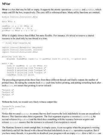
MVarMvar is a box that may be full or empty. It supports the atomic operations takeMVar and putMVar, whichempty and fill the box, respectively. The core API is referenced here. Many utility functions are omitted:

module Control.Concurrent.MVar

data MVar a

newMVar :: a → IO (MVar a)takeMVar :: MVar a → IO aputMVar :: MVar a → a → IO ()

MVar is slightly slower than IORef, but more flexible. For instance, it's trivial to reserve a sharedresource to be used only by one thread at a time:

-- file: mvar-reserve.hs

import Control.Exception (bracket)import Control.Concurrent (forkIO)import Control.Concurrent.MVar

printing lock str = bracket (takeMVar lock)(\i -> putMVar lock $! i+1)(\_ -> print str)

main = do lock <- newMVar () :: IO (MVar ()) forkIO $ printing lock "output a" forkIO $ printing lock "output b" forkIO $ printing lock "output c" takeMVar lock >>= print

The preceding program prints three lines from three different threads and finally outputs the number ofprinted lines. By taking the contents lock MVar each time before printing, and putting something back aftereach print, we ensure that printing is never inlined:

"output a""output b""output c"4

Without the lock, we would very likely witness output like:

"outpu"t"o ouaut"tppuutt bc""

Notice that we used bracket to ensure that we don't reserve the lock indefinitely in case an exception isthrown. This function takes three arguments. The first argument acquires a resource (takeMVar), thesecond releases it (putMVar) and the third does something with the resource between acquire andrelease. bracket ensures that the resource is released if an exception is raised.

The Runtime System is smart enough that, in simple cases, it can recognize when the program is waitingindefinitely and kill the thread with a thread blocked indefinitely in an MVar operation exception. But ifyou have many threads, it is possible to deadlock your program with an empty MVar. Also a full MVar can

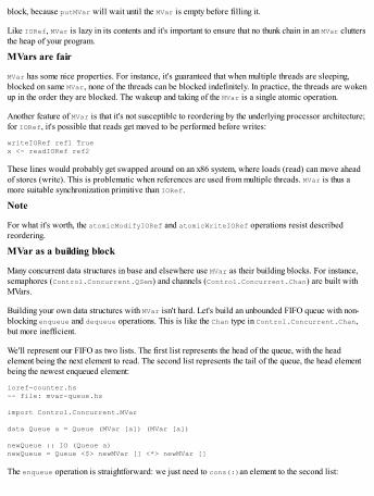
block, because putMVar will wait until the MVar is empty before filling it.

Like IORef, MVar is lazy in its contents and it's important to ensure that no thunk chain in an MVar cluttersthe heap of your program.

MVars are fair

MVar has some nice properties. For instance, it's guaranteed that when multiple threads are sleeping,blocked on same MVar, none of the threads can be blocked indefinitely. In practice, the threads are wokenup in the order they are blocked. The wakeup and taking of the MVar is a single atomic operation.

Another feature of MVar is that it's not susceptible to reordering by the underlying processor architecture;for IORef, it's possible that reads get moved to be performed before writes:

writeIORef ref1 Truex <- readIORef ref2

These lines would probably get swapped around on an x86 system, where loads (read) can move aheadof stores (write). This is problematic when references are used from multiple threads. MVar is thus amore suitable synchronization primitive than IORef.

Note

For what it's worth, the atomicModifyIORef and atomicWriteIORef operations resist describedreordering.

MVar as a building block

Many concurrent data structures in base and elsewhere use MVar as their building blocks. For instance,semaphores (Control.Concurrent.QSem) and channels (Control.Concurrent.Chan) are built withMVars.

Building your own data structures with MVar isn't hard. Let's build an unbounded FIFO queue with non-blocking enqueue and dequeue operations. This is like the Chan type in Control.Concurrent.Chan,but more inefficient.

We'll represent our FIFO as two lists. The first list represents the head of the queue, with the headelement being the next element to read. The second list represents the tail of the queue, the head elementbeing the newest enqueued element:

ioref-counter.hs-- file: mvar-queue.hs

import Control.Concurrent.MVar

data Queue a = Queue (MVar [a]) (MVar [a])

newQueue :: IO (Queue a)newQueue = Queue <$> newMVar [] <*> newMVar []

The enqueue operation is straightforward: we just need to cons(:)an element to the second list:

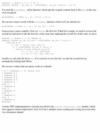
enqueue :: Queue a -> a -> IO ()enqueue (Queue _ ys_var) x = modifyMVar_ ys_var (return . (x :))

I've used the modifyMVar_ utility function, which puts the original contents back to the MVar in the caseof an exception:

modifyMVar_ :: MVar a → (a → IO a) → IO ()

We can also return a result with the modifyMVar function, which we'll use shortly too:

modifyMVar :: MVar a → (a → IO (a, b)) → IO b

Dequeueing is more complex. Now we uncons the first list. If that list is empty, we need to reverse thesecond list and insert it into the first list, at the same time emptying the second list. In the code, we have:

dequeue :: Queue a -> IO (Maybe a)dequeue (Queue xs_var ys_var) = modifyMVar xs_var $ \xs_q -> case xs_q of x : xs -> return (xs, Just x) [] -> modifyMVar ys_var $ \ys_q -> return $ case reverse ys_q of [] -> ([], ([], Nothing)) x : xs -> ([], (xs, Just x))

Usually we only take the first MVar. If we need to reverse the tail, we take the second list too,momentarily locking both MVars.

We can now witness that our queue works as it should:

> q <- newQueue :: IO (Queue Int)> enqueue q 1> enqueue q 2> enqueue q 3> enqueue q 4> dequeue qJust 1> dequeue qJust 2> dequeue qJust 3> dequeue qJust 4> dequeue qNothing

A better FIFO implementation is already provided by the Control.Concurrent.Chan module, whichalso supports channel duplication. Next we'll have multiple actors reading and writing from each othervia a broadcast channel.

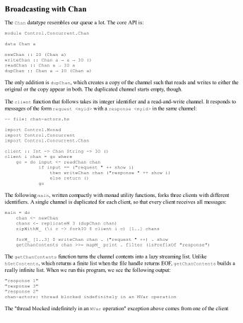
Broadcasting with ChanThe Chan datatype resembles our queue a lot. The core API is:

module Control.Concurrent.Chan

data Chan a

newChan :: IO (Chan a)writeChan :: Chan a → a → IO ()readChan :: Chan a → IO adupChan :: Chan a → IO (Chan a)

The only addition is dupChan, which creates a copy of the channel such that reads and writes to either theoriginal or the copy appear in both. The duplicated channel starts empty, though.

The client function that follows takes its integer identifier and a read-and-write channel. It responds tomessages of the form request <myid> with a response <myid> in the same channel:

-- file: chan-actors.hs

import Control.Monadimport Control.Concurrentimport Control.Concurrent.Chan

client :: Int -> Chan String -> IO ()client i chan = go where go = do input <- readChan chan if input == ("request " ++ show i) then writeChan chan ("response " ++ show i) else return () go

The following main, written compactly with monad utility functions, forks three clients with differentidentifiers. A single channel is duplicated for each client, so that every client receives all messages:

main = do chan <- newChan chans <- replicateM 3 (dupChan chan) zipWithM_ (\i c -> forkIO $ client i c) [1..] chans

forM_ [1..3] $ writeChan chan . ("request " ++) . show getChanContents chan >>= mapM_ print . filter (isPrefixOf "response")

The getChanContents function turns the channel contents into a lazy streaming list. UnlikehGetContents, which returns a finite list when the file handle returns EOF, getChanContents builds areally infinite list. When we run this program, we see the following output:

"response 1""response 3""response 2"chan-actors: thread blocked indefinitely in an MVar operation

The "thread blocked indefinitely in an MVar operation" exception above comes from one of the client

threads. The Runtime System detects that after call to getChanContents, all threads are waiting on thesame Chan and throws anexception. It isn't possible to close a Chan; it will remain open forever.

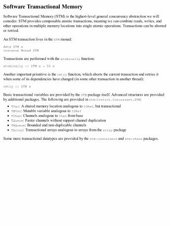
Software Transactional MemorySoftware Transactional Memory (STM) is the highest-level general concurrency abstraction we willconsider. STM provides composable atomic transactions, meaning we can combine reads, writes, andother operations in multiple memory locations into single atomic operations. Transactions can be abortedor retried.

An STM transaction lives in the STM monad:

data STM ainstance Monad STM

Transactions are performed with the atomically function:

atomically :: STM a → IO a

Another important primitive is the retry function, which aborts the current transaction and retries itwhen some of its dependencies have changed (in some other transaction in another thread):

retry :: STM a

Basic transactional variables are provided by the STM package itself. Advanced structures are providedby additional packages. The following are provided in stm:Control.Concurrent.STM:

TVar: A shared memory location analogous to IORef, but transactionalTMVar: Mutable variable analogous to IORefTChan: Channels analogous to Chan from baseTQueue: Faster channels without support channel duplicationTBQueue: Bounded and non-duplicable channelsTArray: Transactional arrays analogous to arrays from the array package

Some more transactional datatypes are provided by the stm-containers and stm-chans packages.

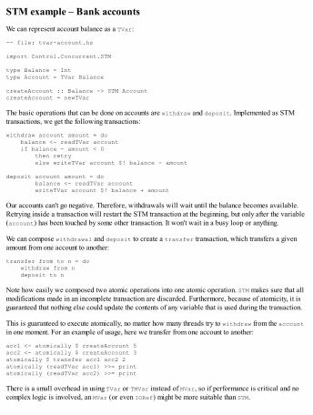
STM example – Bank accountsWe can represent account balance as a TVar:

-- file: tvar-account.hs

import Control.Concurrent.STM

type Balance = Inttype Account = TVar Balance

createAccount :: Balance -> STM AccountcreateAccount = newTVar

The basic operations that can be done on accounts are withdraw and deposit. Implemented as STMtransactions, we get the following transactions:

withdraw account amount = do balance <- readTVar account if balance - amount < 0 then retry else writeTVar account $! balance - amount

deposit account amount = do balance <- readTVar account writeTVar account $! balance + amount

Our accounts can't go negative. Therefore, withdrawals will wait until the balance becomes available.Retrying inside a transaction will restart the STM transaction at the beginning, but only after the variable(account) has been touched by some other transaction. It won't wait in a busy loop or anything.

We can compose withdrawal and deposit to create a transfer transaction, which transfers a givenamount from one account to another:

transfer from to n = do withdraw from n deposit to n

Note how easily we composed two atomic operations into one atomic operation. STM makes sure that allmodifications made in an incomplete transaction are discarded. Furthermore, because of atomicity, it isguaranteed that nothing else could update the contents of any variable that is used during the transaction.

This is guaranteed to execute atomically, no matter how many threads try to withdraw from the accountin one moment. For an example of usage, here we transfer from one account to another:

acc1 <- atomically $ createAccount 5acc2 <- atomically $ createAccount 3atomically $ transfer acc1 acc2 2atomically (readTVar acc1) >>= printatomically (readTVar acc2) >>= print

There is a small overhead in using TVar or TMVar instead of MVar, so if performance is critical and nocomplex logic is involved, an MVar (or even IORef) might be more suitable than STM.

But there are also two even more important caveats that TMVar have over MVar. One is that TMVar isn'tfair; it might take an indefinite time for some thread to unblock on a contended TMVar. Another caveat isdue to overhead from STM, a simple takeTMVar might not be single-wakeup like a takeMVar is, which isa big penalty for highly-contended mutable variables.

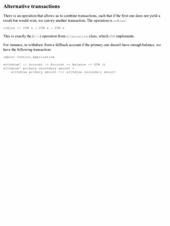
Alternative transactionsThere is an operation that allows us to combine transactions, such that if the first one does not yield aresult but would wait, we can try another transaction. The operation is orElse:

orElse :: STM a → STM a → STM a

This is exactly the (<|>) operation from Alternative class, which STM implements.

For instance, to withdraw from a fallback account if the primary one doesn't have enough balance, wehave the following transaction:

import Control.Applicative

withdraw' :: Account -> Account -> Balance -> STM ()withdraw' primary secondary amount = withdraw primary amount <|> withdraw secondary amount

Exceptions in STMBecause STM is not I/O nor are I/O actions liftable to STM, we cannot use throwIO to throw exceptionswithin an STM transaction. We could use throw or error, but those are asynchronous and don't guaranteeordering respective to other STM operations, like throwIO does for IO.

The correct way to throw exceptions from STM is throwSTM:

throwSTM :: Exception e => e → STM a

And to catch exceptions within STM, we can use catchSTM:

catchSTM :: Exception e => STM a → (e → STM a) → STM a

Alternatively, the MonadThrow/MonadCatch classes from the exceptions package capture correctthrow and catch functions for STM among other monads.

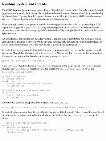
Runtime System and threadsThe GHC Runtime System comes in two flavors: threaded and non-threaded. For truly single-threadedapplications, it's usually better to use the default non-threaded runtime, because there's more overhead inthe threaded one. The non-threaded runtime features a scheduler for light-weight GHC threads (createdvia forkIO), providing for single-threaded concurrent programming.

Usually though, a concurrent program benefits from being multi-threaded – that is, using multiple CPUcapabilities triggered via the -N<n> RTS flag when compiled with -threaded. The Runtime Systemcreates one system thread for every capability and schedules light-weight threads to run in parallel on itssystem threads.

An important caveat with the non-threaded runtime is that if a light-weight thread has blocked a systemcall, the whole program will block. On the threaded runtime, GHC can schedule light-weight threads torun on other system threads while the other thread is blocked on a system call.

In Haskell, threads are identified by their ThreadId. One is returned by forkIO to the main thread, andthe current ThreadId can be retrieved with myThreadId. We can use this ThreadId to throw exceptionsfrom any thread to any other thread asynchronously, using throwTo:

throwTo :: Exception e => ThreadId → e → IO ()

The killThread function throws a ThreadKilled exception to the target thread. The forkIO functiondiscards the ThreadKilled exception (also the exceptions BlockedIndefinitelyOnMVar andBlockedIndefinitelyOnSTM):

-- file: forking.hs-- outputs nothingtest1 = do tid <- forkIO $ threadDelay 100000000 killThread tid

-- outputs exception: Prelude.undefinedtest2 = do tid <- forkIO $ undefined killThread tid

If you need to catch all exceptions from a thread, use forkFinally:

forkFinally :: IO a → (Either SomeException a → IO ()) → IO ThreadId

In Haskell, when the main thread exits, all child threads are killed as well. Often it's useful to wait for allthreads to exit, or inform some other thread when a thread dies. For this, forkFinally is the perfectutility:

-- waits for the child thread to exittest3 = do mvar <- newEmptyMVar tid <- threadDelay 5000000 `forkFinally` \_ -> putMVar mvar () takeMVar mvar

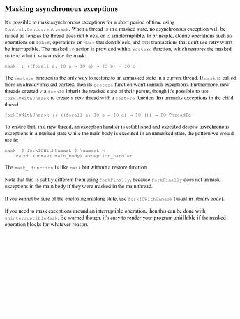
Masking asynchronous exceptionsIt's possible to mask asynchronous exceptions for a short period of time usingControl.Concurrent.mask. When a thread is in a masked state, no asynchronous exception will beraised as long as the thread does not block, or is uninterruptible. In principle, atomic operations such asoperations on IORef, operations on MVar that don't block, and STM transactions that don't use retry won'tbe interruptible. The masked IO action is provided with a restore function, which restores the maskedstate to what it was outside the mask:

mask :: ((forall a. IO a → IO a) → IO b) → IO b

The restore function is the only way to restore to an unmasked state in a current thread. If mask is calledfrom an already masked context, then its restore function won't unmask exceptions. Furthermore, newthreads created via forkIO inherit the masked state of their parent, though it's possible to useforkIOWithUnmask to create a new thread with a restore function that unmasks exceptions in the childthread:

forkIOWithUnmask :: ((forall a. IO a → IO a) → IO ()) → IO ThreadId

To ensure that, in a new thread, an exception handler is established and executed despite asynchronousexceptions in a masked state while the main body is executed in an unmasked state, the pattern we woulduse is:

mask_ $ forkIOWithUnmask $ \unmask → catch (unmask main_body) exception_handler

The mask_ function is like mask but without a restore function.

Note that this is subtly different from using forkFinally, because forkFinally does not unmaskexceptions in the main body if they were masked in the main thread.

If you cannot be sure of the enclosing masking state, use forkIOWithUnmask (usual in library code).

If you need to mask exceptions around an interruptible operation, then this can be done withuninterruptibleMask. Be warned though, it's easy to render your program unkillable if the maskedoperation blocks for whatever reason.

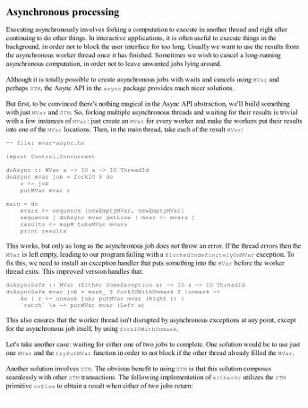
Asynchronous processingExecuting asynchronously involves forking a computation to execute in another thread and right aftercontinuing to do other things. In interactive applications, it is often useful to execute things in thebackground, in order not to block the user interface for too long. Usually we want to use the results fromthe asynchronous worker thread once it has finished. Sometimes we wish to cancel a long-runningasynchronous computation, in order not to leave unwanted jobs lying around.

Although it is totally possible to create asynchronous jobs with waits and cancels using MVar andperhaps STM, the Async API in the async package provides much nicer solutions.

But first, to be convinced there's nothing magical in the Async API abstraction, we'll build somethingwith just MVar and STM. So, forking multiple asynchronous threads and waiting for their results is trivialwith a few instances of MVar: just create an MVar for every worker and make the workers put their resultsinto one of the MVar locations. Then, in the main thread, take each of the result MVar:

-- file: mvar-async.hs

import Control.Concurrent

doAsync :: MVar a -> IO a -> IO ThreadIddoAsync mvar job = forkIO $ do r <- job putMVar mvar r

main = do mvars <- sequence [newEmptyMVar, newEmptyMVar] sequence [ doAsync mvar getLine | mvar <- mvars ] results <- mapM takeMVar mvars print results

This works, but only as long as the asynchronous job does not throw an error. If the thread errors then theMVar is left empty, leading to our program failing with a BlockedIndefinitelyOnMVar exception. Tofix this, we need to install an exception handler that puts something into the MVar before the workerthread exits. This improved version handles that:

doAsyncSafe :: MVar (Either SomeException a) -> IO a -> IO ThreadIddoAsyncSafe mvar job = mask_ $ forkIOWithUnmask $ \unmask -> do { r <- unmask job; putMVar mvar (Right r) } `catch` \e -> putMVar mvar (Left e)

This also ensures that the worker thread isn't disrupted by asynchronous exceptions at any point, exceptfor the asynchronous job itself, by using forkIOWithUnmask.

Let's take another case: waiting for either one of two jobs to complete. One solution would be to use justone MVar and the tryPutMVar function in order to not block if the other thread already filled the MVar.

Another solution involves STM. The obvious benefit to using STM is that this solution composesseamlessly with other STM transactions. The following implementation of eitherOr utilizes the STMprimitive orElse to obtain a result when either of two jobs return:

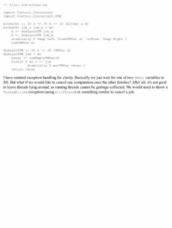
-- file: stm-either.hs

import Control.Concurrentimport Control.Concurrent.STM

eitherOr :: IO a -> IO b -> IO (Either a b)eitherOr job_a job_b = do a <- doAsyncSTM job_a b <- doAsyncSTM job_b atomically $ fmap Left (takeTMVar a) `orElse` fmap Right ( takeTMVar b)

doAsyncSTM :: IO a -> IO (TMVar a)doAsyncSTM job = do tmvar <- newEmptyTMVarIO forkIO $ do r <- job atomically $ putTMVar tmvar r return tmvar

I have omitted exception handling for clarity. Basically we just wait for one of two TMVar variables tofill. But what if we would like to cancel one computation once the other finishes? After all, it's not goodto leave threads lying around, as running threads cannot be garbage-collected. We would need to throw aThreadKilled exception (using killThread) or something similar to cancel a job.

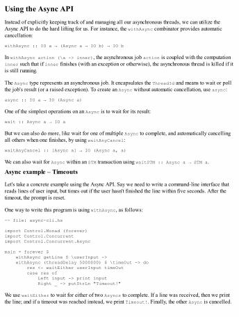
Using the Async APIInstead of explicitly keeping track of and managing all our asynchronous threads, we can utilize theAsync API to do the hard lifting for us. For instance, the withAsync combinator provides automaticcancellation:

withAsync :: IO a → (Async a → IO b) → IO b

In withAsync action (\a -> inner), the asynchronous job action is coupled with the computationinner such that if inner finishes (with an exception or otherwise), the asynchronous thread is killed if itis still running.

The Async type represents an asynchronous job. It encapsulates the ThreadId and means to wait or pollthe job's result (or a raised exception). To create an Async without automatic cancellation, use async:

async :: IO a → IO (Async a)

One of the simplest operations on an Async is to wait for its result:

wait :: Async a → IO a

But we can also do more, like wait for one of multiple Async to complete, and automatically cancellingall others when one finishes, by using waitAnyCancel:

waitAnyCancel :: [Async a] → IO (Async a, a)

We can also wait for Async within an STM transaction using waitSTM :: Async a → STM a.

Async example – Timeouts

Let's take a concrete example using the Async API. Say we need to write a command-line interface thatreads lines of user input, but times out if the user hasn't finished the line within five seconds. After thetimeout, the prompt is reset.

One way to write this program is using withAsync, as follows:

-- file: async-cli.hs

import Control.Monad (forever)import Control.Concurrentimport Control.Concurrent.Async

main = forever $ withAsync getLine $ \userInput -> withAsync (threadDelay 5000000) $ \timeOut -> do res <- waitEither userInput timeOut case res of Left input -> print input Right _ -> putStrLn "Timeout!"

We use waitEither to wait for either of two Asyncs to complete. If a line was received, then we printthe line; and if a timeout was reached instead, we print Timeout!. Finally, the other Async is cancelled.

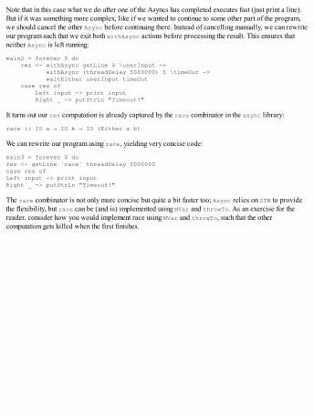
Note that in this case what we do after one of the Asyncs has completed executes fast (just print a line).But if it was something more complex, like if we wanted to continue to some other part of the program,we should cancel the other Async before continuing there. Instead of cancelling manually, we can rewriteour program such that we exit both withAsync actions before processing the result. This ensures thatneither Async is left running:

main2 = forever $ do res <- withAsync getLine $ \userInput -> withAsync (threadDelay 5000000) $ \timeOut -> waitEither userInput timeOut case res of Left input -> print input Right _ -> putStrLn "Timeout!"

It turns out our res computation is already captured by the race combinator in the async library:

race :: IO a → IO b → IO (Either a b)

We can rewrite our program using race, yielding very concise code:

main3 = forever $ dores <- getLine `race` threadDelay 5000000case res ofLeft input -> print inputRight _ -> putStrLn "Timeout!"

The race combinator is not only more concise but quite a bit faster too; Async relies on STM to providethe flexibility, but race can be (and is) implemented using MVar and throwTo. As an exercise for thereader, consider how you would implement race using MVar and throwTo, such that the othercomputation gets killed when the first finishes.

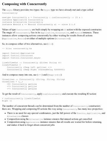
Composing with ConcurrentlyThe async library provides two types: the Async type we have already met and a type calledConcurrently:

newtype Concurrently a = Concurrently { runConcurrently :: IO a }instance Applicative Concurrentlyinstance Alternative Concurrentlyinstance Monoid a => Monoid (Concurrently a) -- since 2.1.0

Values of type Concurrently are built simply by wrapping an IO action with the exposed constructor.The magic of Concurrently lies in its Applicative, Alternative, and Monoid instances. Theseinstances allow composing actions concurrently by either waiting for results from all actions(Applicative, Monoid) or either of multiple options (Alternative).

So, to compose either of two alternatives, use (<|>):

-- file: concurrently.hs

import Control.Applicativeimport Control.Concurrentimport Control.Concurrent.Async

lineOrTimeOut :: Concurrently (Either String ())lineOrTimeOut = Concurrently (fmap Left getLine) <|> Concurrently (fmap Right (threadDelay 5000000))

And to compose many into one, use (<*>) and (fmap/(<$>)):

threeLines :: Concurrently (String, String, String)threeLines = (,,) <$> Concurrently getLine <*> Concurrently getLine <*> Concurrently getLine

To get the result of Concurrently, apply runConcurrently and execute the resulting IO action:

> runConcurrently lineOrTimeOut Right ()

The number of concurrent threads can be determined from the number of Concurrently constructorsthere are. Wrapping and composing IO actions this way using Concurrently has many nice properties:

There is no need for any special combinators, just the full power of the Functor, Applicative, andAlternative classesComposition using the Alternative instance ensures that unused actions get cancelledComposition using Applicative instance ensures that all results are waited for before returning,and makes it hard to forget about concurrent jobs

Lifting up from I/OIn real-world applications, it's quite usual for much of the code base to live in monads or monad stacks.In such situations, concurrency operations from Control.Concurrent become challenging, because theyall are monomorphic in IO. Sometimes this isn't much of a problem, because we can use liftIO from theMonadIO class to lift arbitrary IO actions.

But MonadIO leaves two important cases uncovered. The first one is about other base monads besides IO,such as STM. Though more limited in its use cases, it's sometimes desired to have a monad stack on top ofSTM. The other case is about exception handling, for which MonadIO is quite insufficient; all ofControl.Exception is monomorphic in IO, meaning a lot of plumbing if they are used within a monadstack.

In this chapter, we'll look at some solutions to both cases. Another thing that's often desired, and whichwe'll cover first, is top-level mutable references. In some languages these are called globals, andthough they're often shunned, Haskell kind of supports them but in a way that's more useful.

Top-level mutable referencesAll references (IORef, MVar, TVar) are created in the IO or STM monad. It is possible to escape IO usingunsafePerformIO, and it's safe to do so when used correctly. One such safe use is at top-levelaccompanied with a NOINLINE pragma:

-- file: top-level.hsoimport Data.IORefimport System.IO.Unsafe (unsafePerformIO)

globalVariable :: IORef StringglobalVariable = unsafePerformIO (newIORef ""){-# NOINLINE globalVariable #-}

It's important to set the variable to non-inlinable, because if it inlines, a new IORef might get created onreference. Equally important is to ensure the top-level variable has a monomorphic type. For instance,this is bad:

globalVar :: Num a => IORef aglobalVar = unsafePerformIO (newIORef 0)

Even if globalVar is not inlined, it now represents a function (with an implicit class dictionaryparameter). Effectively this means that a new IORef is created every time we reference globalVar.

When it comes to transactional variables in STM, it should be noted that atomically cannot be usedinside unsafePerformIO (weird things will happen). Instead, the IO variations should be used, such asnewTVarIO which lives in IO and can be used with unsafePerformIO. The same considerations aboutinlining and monomorphic typing apply for transactional top-level variables as well.

Lifting from a base monadThe transformers library provides the MonadIO class to lift from base IO. With base we mean thebottom monad of a monad transformer stack. The transformers-base, library, on the other hand,provides a MonadBase class to lift from an arbitrary base:

class MonadBase b m | m → b where liftBase :: b a → m a

Type variable b represents the base (for example, IO) and m is the monad to lift operations to. ForMonadBase IO, liftBase is equivalent to liftIO. The benefits of MonadBase are mostly in its otherbase instances, such as STM or ST. For instance, if we were writing complex STM transactions and wantedto wrap some common data with a Reader monad on top of STM:

-- file: transactionm.hs

import Control.Monad.Baseimport Control.Monad.Trans.Readerimport Control.Concurrent.STM

type TransactionM a = ReaderT String STM a

To lift STM transactions to TransactionM, we could use Control.Monad.Trans.lift. But if the stackwas bigger, we would end up doing lift . lift . lift or similar, and if we instead had ourTransactionM be a newtype, it would be impossible to lift STM operations into it using lift. By usingliftBase, we can circumvent both of these restrictions, because a single liftBase will lift through anarbitrary stack as long as the base monad is sitting at the bottom.

The newtype case is straightforward; we can derive the instance for MonadBase:

{-# LANGUAGE GeneralizedNewtypeDeriving #-}

newtype TransactionM' a = TransactionM' (ReaderT String STM a) deriving ( Functor, Applicative, Monad , MonadReader String, MonadBase STM )

If on the other hand you don't need the full power of STM, then the stm-lifted library provides basicatomic operations such as readTVarIO, dupTChanIO, and so forth on transactional variables lifted intoMonadIO.

Lifting base with exception handlingLifting operations using MonadBase was very similar to MonadIO, just more general in the base monad.But lifting operations from Control.Concurrent is trickier. For instance, how do we lift forkIO into,say, WriterT Int IO? We have to decide what happens with the added state from the transformers. Inthe case of forkIO, that's simple: just duplicate the current state into the new thread. But how about anexception handler of catch?

catch :: Exception e => IO a → (e → IO a) → IO a

A generalized version of catch provided by the lifted-base package has this signature:

module Control.Exception.Lifted

catch :: (MonadBaseControl IO m, Exception e) => m a → (e → m a) → m a

Like MonadBase, MonadBaseControl is a type class that allows lifting operations from the base monad.As the name implies, MonadBaseControl adds something extra to the lifting. The type class definition isalso entirely different from MonadBase:

class MonadBase b m => MonadBaseControl b m | m → b where type StM m a :: * liftBaseWith :: (RunInBase m b → b a) → m a restoreM :: StM m a → m a

Fortunately, it isn't necessary to understand how this class works in order to use MonadBaseControl; interms of user interface, it looks just like MonadBase (or indeed MonadIO).

But what is useful to understand is the main implication of MonadBaseControl, namely that it saves theadded monadic state (as a value of associated type StM m a) and uses this saved state to runcomputations such as the exception handler in catch. This means that the computation in an exceptionhandler is executed using the monadic state before calling catch. What's more, the monadic state from acomputation that throws an exception is also discarded.

Apart from generalizing Control.Concurrent and Control.Exception with module names suffixedwith Lifted, in the lifted-base library there are generalized versions of some other modules in baseas well, including, for example, Data.IORef.Lifted. Some functions generalize well with justMonadBase IO, and those are left as such. Others that require monadic state controlling are marked withMonadBaseControl in their type signatures.

Because of the associated type in MonadBaseControl class, making an instance for a newtype issubstantially harder than MonadBase. Sadly, GHC won't derive any instances for classes with associatedtypes, and the higher-order class functions sure aren't making our lives any easier.

For reference, here's an example of a manually-written derived instance for a newtyped monad stack:

-- file: newtype-monadbasecontrol.hs

newtype Handler a = Handler { unHandler :: LoggingT (StateT HandlerState (ReaderT Config IO)) a

} deriving ( ... )

instance MonadBaseControl IO Handler where type StM Handler a = StM(LoggingT (StateT HandlerState (ReaderT Config IO))) a

liftBaseWith f = Handler $ liftBaseWith $ \q -> f (q . unHandler)

restoreM = Handler . RestoreM

SummaryIn this chapter, we started by looking at light-weight threads and forkIO. Closely related to this, welooked at mutable references IORef and MVar in concurrent settings. Atomic operations on thosereference types were quite limited, which is why we next dived into STM for arbitrarily complextransactions. Then we considered a nice higher-level abstraction over an asynchronous program, theAsync API. One of the main benefits of using Async is easy and automatic cancellation of asynchronousjobs. Finally, we lifted concurrency operations into complex monad stacks.

In the next chapter, we will take a deeper look at the Runtime System, scheduling, and garbage collection.We will look at what options there are to tweak both the compiler and the Runtime System. We will learnhow the GHC compilation pipeline works and how to read the intermediate core language that GHCproduces just enough to spot possibly missed optimizations.

Chapter 8. Tweaking the Compiler and Runtime System (GHC)In the previous chapter, we got programmed concurrent applications and used the related powerfulfeatures of GHC. Next we concentrate on tuning GHC and its Runtime System. For the best performance,it's necessary to tune the compiler and Runtime System according to the application's specific needs. Forinstance, heavy number crunching benefits greatly from a different compilation path using LLVM, at theexpense of longer compilation times and portability. There are lots of useful options, tricks, and tweaksavailable in GHC that we will look at in this chapter.

This chapter attempts to highlight the most important flags and options in GHC and RTS. It's not meant tobe a substitute for GHC UserGuide, which is much more comprehensive. Instead, we cover options in asystematic and easy-to-follow way, starting with compiler options and proceeding with Runtime Systemoptions.

At the end of this chapter, the reader will understand the big picture of compiler phases in GHC and themost important options that affect compilation, optimization, code generations, linking, and preprocessingin GHC. The reader will be familiar with the Runtime System, its scheduler, green threads, memorymanagement, and the garbage collector. We will mention some important configuration options that affectRuntime System performance or enable tracing features.

An additional Haskell feature more or less related to GHC is Safe Haskell, which helps programmers intrusting libraries to do what they promise. In essence, Safe Haskell enforces referential transparency: aSafe Haskell module cannot use unsafePerformIO, for example. In this chapter, we will learn how SafeHaskell can help in trusting code and validating it We will take a look at the following topics:.

Compiling and linking with GHCConfiguring and tuning GHC and the Runtime SystemCompiling safely with Safe HaskellUnderstanding memory management, GC, and scheduler in Runtime System

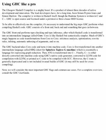
Using GHC like a proThe Glasgow Haskell Compiler is a mighty beast. It's a product of almost three decades of activedevelopment and innovation. The lead developers have, for a long time, been Simon Peyton Jones andSimon Marlow. The compiler is written in Haskell itself, though the Runtime System is written in C andC--. GHC is open source and licensed under a permissive three-clause BSD license.

To be able to effectively use the compiler, it's necessary to understand the big steps GHC performs whencompiling Haskell code. GHC consists of a front end, back end and something that goes in-between.

The GHC front end performs type-checking and type inference, after which Haskell code is transformedinto an intermediate language called Core. Core is like Haskell but syntactically simpler. Much of GHC'smagic happens as code transformations from Core to Core: strictness analysis, optimization, rewriterules, inlining, automatic unboxing of arguments, and so on.

The GHC backend takes Core code and turns it into machine code. Core is first transformed into anotherintermediate language called STG (short for Spineless Tagless G-machine) which is essentially alanguage for expressing graph reduction. Then, STG is transformed into C--. Finally, C-- is eitherdirectly converted into machine code using GHC's native code generator, converted to LLVM code forcompilation with LLVM, or printed as C code to be compiled with GCC. However, the C route isgenerally deprecated and is not included in usual builds of GHC (it may still be used for cross-compiling).

Next, we will consider the most important GHC flags and common use cases. For a complete overview,consult the GHC UserGuide.

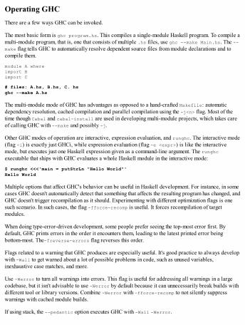
Operating GHCThere are a few ways GHC can be invoked.

The most basic form is ghc program.hs. This compiles a single-module Haskell program. To compile amulti-module program, that is, one that consists of multiple .hs files, use ghc --make Main.hs. The --make flag tells GHC to automatically resolve dependent source files from module declarations and tocompile them.

module A whereimport Bimport C

# files: A.hs, B.hs, C. hsghc --make A.hs

The multi-module mode of GHC has advantages as opposed to a hand-crafted Makefile: automaticdependency resolution, cached compilation and parallel compilation using the -j<n> flag. Most of thetime though Cabal and cabal-install are used in developing multi-module projects, which takes careof calling GHC with --make and possibly -j.

Other GHC modes of operation are interactive, expression evaluation, and runghc. The interactive mode(flag -i) is exactly just GHCi, while expression evaluation (flag -e <expr>) is like the interactivemode, but executes just one Haskell expression given as a command-line argument. The runghcexecutable that ships with GHC evaluates a whole Haskell module in the interactive mode:

$ runghc <<<'main = putStrLn "Hello World"'Hello World

Multiple options that affect GHC's behavior can be useful in Haskell development. For instance, in somecases GHC doesn't automatically detect that something that affects the resulting program has changed, andGHC doesn't trigger recompilation as it should. Experimenting with different optimization flags is onesuch scenario. In such cases, the flag -fforce-recomp is useful. It forces recompilation of targetmodules.

When doing type-error-driven development, some people prefer seeing the top-most error first. Bydefault, GHC prints errors in the order it encounters them, leading to the latest printed error beingbottom-most. The-freverse-errors flag reverses this order.

Flags related to a warning that GHC produces are especially useful. It's good practice to always developwith -Wall to get warned about a lot of possible problems in code, such as unused variables,inexhaustive case matches, and more.

Use -Werror to turn all warnings into errors. This flag is useful for addressing all warnings in a largecodebase, but it isn't advisable to use -Werror by default because it can unnecessarily break builds withdifferent tool or library versions. Combine -Werror with -fforce-recomp to not silently suppresswarnings with cached module builds.

If using stack, the --pedantic option executes GHC with -Wall -Werror.

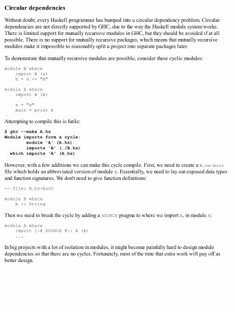
Circular dependencies

Without doubt, every Haskell programmer has bumped into a circular dependency problem. Circulardependencies are not directly supported by GHC, due to the way the Haskell module system works.There is limited support for mutually recursive modules in GHC, but they should be avoided if at allpossible. There is no support for mutually recursive packages, which means that mutually recursivemodules make it impossible to reasonably split a project into separate packages later.

To demonstrate that mutually recursive modules are possible, consider these cyclic modules:

module B where import A (a) b = a ++ "b"

module A where import B (b) a = "a" main = print b

Attempting to compile this is futile:

$ ghc --make A.hsModule imports form a cycle: module 'A' (A.hs) imports 'B' (./B.hs) which imports 'A' (A.hs)

However, with a few additions we can make this cycle compile. First, we need to create a B.hs-bootfile which holds an abbreviated version of module B. Essentially, we need to lay out exposed data typesand function signatures. We don't need to give function definitions:

-- file: B.hs-boot

module B where b :: String

Then we need to break the cycle by adding a SOURCE pragma to where we import B, in module A:

module A where import {-# SOURCE #-} B (b) ...

In big projects with a lot of isolation in modules, it might become painfully hard to design moduledependencies so that there are no cycles. Fortunately, most of the time that extra work will pay off asbetter design.

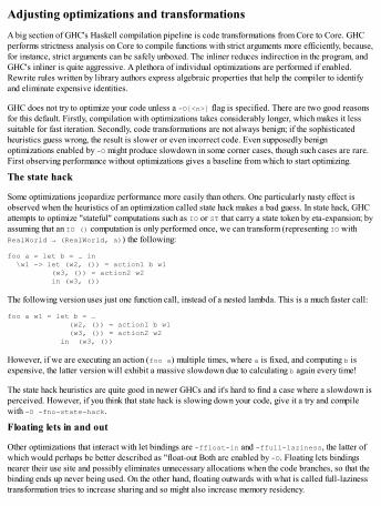
Adjusting optimizations and transformationsA big section of GHC's Haskell compilation pipeline is code transformations from Core to Core. GHCperforms strictness analysis on Core to compile functions with strict arguments more efficiently, because,for instance, strict arguments can be safely unboxed. The inliner reduces indirection in the program, andGHC's inliner is quite aggressive. A plethora of individual optimizations are performed if enabled.Rewrite rules written by library authors express algebraic properties that help the compiler to identifyand eliminate expensive identities.

GHC does not try to optimize your code unless a -O[<n>] flag is specified. There are two good reasonsfor this default. Firstly, compilation with optimizations takes considerably longer, which makes it lesssuitable for fast iteration. Secondly, code transformations are not always benign; if the sophisticatedheuristics guess wrong, the result is slower or even incorrect code. Even supposedly benignoptimizations enabled by -O might produce slowdown in some corner cases, though such cases are rare.First observing performance without optimizations gives a baseline from which to start optimizing.

The state hack

Some optimizations jeopardize performance more easily than others. One particularly nasty effect isobserved when the heuristics of an optimization called state hack makes a bad guess. In state hack, GHCattempts to optimize "stateful" computations such as IO or ST that carry a state token by eta-expansion; byassuming that an IO () computation is only performed once, we can transform (representing IO withRealWorld → (RealWorld, a)) the following:

foo a = let b = … in \w1 -> let (w2, ()) = action1 b w1 (w3, ()) = action2 w2 in (w3, ())

The following version uses just one function call, instead of a nested lambda. This is a much faster call:

foo a w1 = let b = … (w2, ()) = action1 b w1 (w3, ()) = action2 w2 in (w3, ())

However, if we are executing an action (foo a) multiple times, where a is fixed, and computing b isexpensive, the latter version will exhibit a massive slowdown due to calculating b again every time!

The state hack heuristics are quite good in newer GHCs and it's hard to find a case where a slowdown isperceived. However, if you think that state hack is slowing down your code, give it a try and compilewith -O -fno-state-hack.

Floating lets in and out

Other optimizations that interact with let bindings are -ffloat-in and -ffull-laziness, the latter ofwhich would perhaps be better described as "float-out Both are enabled by -O. Floating lets bindingsnearer their use site and possibly eliminates unnecessary allocations when the code branches, so that thebinding ends up never being used. On the other hand, floating outwards with what is called full-lazinesstransformation tries to increase sharing and so might also increase memory residency.

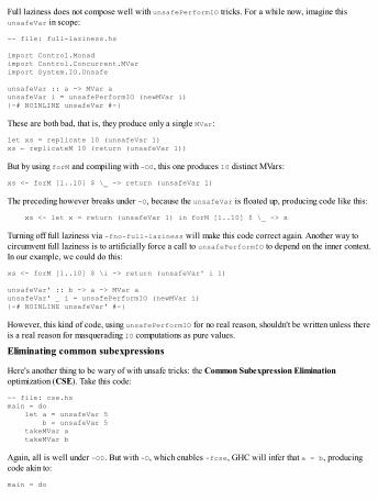
Full laziness does not compose well with unsafePerformIO tricks. For a while now, imagine thisunsafeVar in scope:

-- file: full-laziness.hs

import Control.Monadimport Control.Concurrent.MVarimport System.IO.Unsafe

unsafeVar :: a -> MVar aunsafeVar i = unsafePerformIO (newMVar i){-# NOINLINE unsafeVar #-}

These are both bad, that is, they produce only a single MVar:

let xs = replicate 10 (unsafeVar 1)xs ← replicateM 10 (return (unsafeVar 1))

But by using forM and compiling with -O0, this one produces 10 distinct MVars:

xs <- forM [1..10] $ \_ -> return (unsafeVar 1)

The preceding however breaks under -O, because the unsafeVar is floated up, producing code like this:

xs <- let x = return (unsafeVar 1) in forM [1..10] $ \_ -> x

Turning off full laziness via -fno-full-laziness will make this code correct again. Another way tocircumvent full laziness is to artificially force a call to unsafePerformIO to depend on the inner context.In our example, we could do this:

xs <- forM [1..10] $ \i -> return (unsafeVar' i 1)

unsafeVar' :: b -> a -> MVar aunsafeVar' _ i = unsafePerformIO (newMVar i){-# NOINLINE unsafeVar' #-}

However, this kind of code, using unsafePerformIO for no real reason, shouldn't be written unless thereis a real reason for masquerading IO computations as pure values.

Eliminating common subexpressions

Here's another thing to be wary of with unsafe tricks: the Common Subexpression Eliminationoptimization (CSE). Take this code:

-- file: cse.hsmain = do let a = unsafeVar 5 b = unsafeVar 5 takeMVar a takeMVar b

Again, all is well under -O0. But with -O, which enables -fcse, GHC will infer that a = b, producingcode akin to:

main = do

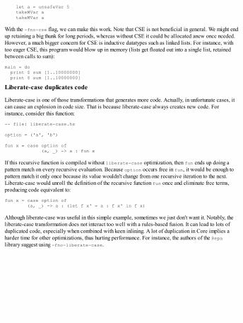
let a = unsafeVar 5 takeMVar a takeMVar a

With the -fno-cse flag, we can make this work. Note that CSE is not beneficial in general. We might endup retaining a big thunk for long periods, whereas without CSE it could be allocated anew once needed.However, a much bigger concern for CSE is inductive datatypes such as linked lists. For instance, withtoo eager CSE, this program would blow up in memory (lists get floated out into a single list, retainedbetween calls to sum):

main = do print $ sum [1..10000000] print $ sum [1..10000000]

Liberate-case duplicates code

Liberate-case is one of those transformations that generates more code. Actually, in unfortunate cases, itcan cause an explosion in code size. That is because liberate-case always creates new code. Forinstance, consider this function:

-- file: liberate-case.hs

option = ('a', 'b')

fun x = case option of (a, _) -> a : fun x

If this recursive function is compiled without liberate-case optimization, then fun ends up doing apattern match on every recursive evaluation. Because option occurs free in fun, it would be enough topattern match it only once because its value wouldn't change from one recursive iteration to the next.Liberate-case would unroll the definition of the recursive function fun once and eliminate free terms,producing code equivalent to:

fun x = case option of (a, _) -> a : (let f x' = a : f x' in f x)

Although liberate-case was useful in this simple example, sometimes we just don't want it. Notably, theliberate-case transformation does not interact too well with a rules-based fusion. It can lead to lots ofduplicated code, especially when combined with keen inlining. A lot of duplication in Core implies aharder time for other optimizations, thus hurting performance. For instance, the authors of the Repalibrary suggest using -fno-liberate-case.

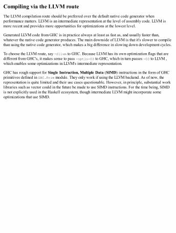
Compiling via the LLVM routeThe LLVM compilation route should be preferred over the default native code generator whenperformance matters. LLVM is an intermediate representation at the level of assembly code. LLVM ismore recent and provides more opportunities for optimizations at the lowest level.

Generated LLVM code from GHC is in practice always at least as fast as, and usually faster than,whatever the native code generator produces. The main downside of LLVM is that it's slower to compilethan using the native code generator, which makes a big difference in slowing down development cycles.

To choose the LLVM route, say -fllvm to GHC. Because LLVM has its own optimization flags that aredifferent from GHC's, it makes sense to pass -optlo-O3 to GHC, which in turn passes -O3 to LLVM ,which enables some optimizations in LLVM's intermediate representation.

GHC has rough support for Single Instruction, Multiple Data (SIMD) instructions in the form of GHCprimitives defined in GHC.Prim module. They only work if using the LLVM backend. As of now, therepresentation is quite limited and their use cases questionable. However, in principle, substantial worklibraries such as vector could in the future be made to use SIMD instructions. For the time being, SIMDis not explicitly used in the Haskell ecosystem, though intermediate LLVM might incorporate someoptimizations that use SIMD.

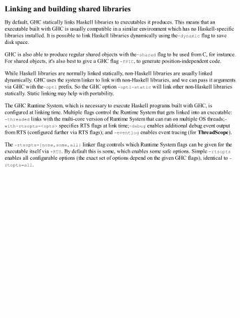
Linking and building shared librariesBy default, GHC statically links Haskell libraries to executables it produces. This means that anexecutable built with GHC is usually compatible in a similar environment which has no Haskell-specificlibraries installed. It is possible to link Haskell libraries dynamically using the-dynamic flag to savedisk space.

GHC is also able to produce regular shared objects with the-shared flag to be used from C, for instance.For shared objects, it's also best to give a GHC flag -fPIC, to generate position-independent code.

While Haskell libraries are normally linked statically, non-Haskell libraries are usually linkeddynamically. GHC uses the system linker to link with non-Haskell libraries, and we can pass it argumentsvia GHC with the-optl prefix. So the GHC option -optl-static will link other non-Haskell librariesstatically. Static linking may help with portability.

The GHC Runtime System, which is necessary to execute Haskell programs built with GHC, isconfigured at linking time. Multiple flags control the Runtime System that gets linked into an executable:-threaded links with the multi-core version of Runtime System that can run on multiple OS threads;-with-rtsopts=<opts> specifies RTS flags at link time;-debug enables additional debug event outputfrom RTS (configured further via RTS flags); and -eventlog enables event tracing (for ThreadScope).

The -rtsopts={none,some,all} linker flag controls which Runtime System flags can be given for theexecutable itself via +RTS. By default this is some, which enables some safe options. Simple -rtsoptsenables all configurable options (the exact set of options depend on the given GHC flags), identical to -rtopts=all.

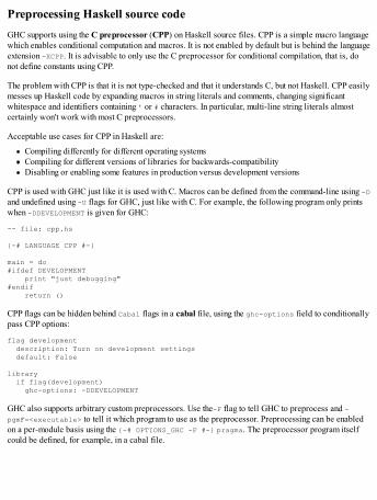
Preprocessing Haskell source codeGHC supports using the C preprocessor (CPP) on Haskell source files. CPP is a simple macro languagewhich enables conditional computation and macros. It is not enabled by default but is behind the languageextension -XCPP. It is advisable to only use the C preprocessor for conditional compilation, that is, donot define constants using CPP.

The problem with CPP is that it is not type-checked and that it understands C, but not Haskell. CPP easilymesses up Haskell code by expanding macros in string literals and comments, changing significantwhitespace and identifiers containing ' or # characters. In particular, multi-line string literals almostcertainly won't work with most C preprocessors.

Acceptable use cases for CPP in Haskell are:

Compiling differently for different operating systemsCompiling for different versions of libraries for backwards-compatibilityDisabling or enabling some features in production versus development versions

CPP is used with GHC just like it is used with C. Macros can be defined from the command-line using -Dand undefined using -U flags for GHC, just like with C. For example, the following program only printswhen -DDEVELOPMENT is given for GHC:

-- file: cpp.hs

{-# LANGUAGE CPP #-}

main = do#ifdef DEVELOPMENT print "just debugging"#endif return ()

CPP flags can be hidden behind Cabal flags in a cabal file, using the ghc-options field to conditionallypass CPP options:

flag development description: Turn on development settings default: False

library if flag(development) ghc-options: -DDEVELOPMENT

GHC also supports arbitrary custom preprocessors. Use the-F flag to tell GHC to preprocess and -pgmF=<executable> to tell it which program to use as the preprocessor. Preprocessing can be enabledon a per-module basis using the {-# OPTIONS_GHC -F #-} pragma. The preprocessor program itselfcould be defined, for example, in a cabal file.

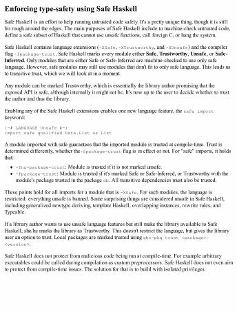
Enforcing type-safety using Safe HaskellSafe Haskell is an effort to help running untrusted code safely. It's a pretty unique thing, though it is stillbit rough around the edges. The main purposes of Safe Haskell include to machine-check untrusted code,define a safe subset of Haskell that cannot use unsafe functions, call foreign C, or hang the system.

Safe Haskell contains language extensions (-XSafe, -XTrustworthy, and -XUnsafe) and the compilerflag -fpackage-trust. Safe Haskell marks every module either Safe, Trustworthy, Unsafe, or Safe-Inferred. Only modules that are either Safe or Safe-Inferred are machine-checked to use only safelanguage. However, safe modules may still use modules that don't fit to only safe language. This leads usto transitive trust, which we will look at in a moment.

Any module can be marked Trustworthy, which is essentially the library author promising that theexposed API is safe, although internally it might not be. It's now up to the user to decide whether to trustthe author and thus the library.

Enabling any of the Safe Haskell extensions enables one new language feature, the safe importkeyword:

{-# LANGUAGE Unsafe #-}import safe qualified Data.List as List

A module imported with safe guarantees that the imported module is trusted at compile-time. Trust isdetermined differently, whether the-fpackage-trust flag is in effect or not. For "safe" imports, it holdsthat:

-fno-package-trust: Module is trusted if it is not marked unsafe.-fpackage-trust: Module is trusted if it's marked Safe or Safe-Inferred, or Trustworthy with themodule's package trusted in the package db. All transitive dependencies must also be trusted.

These points hold for all imports for a module that is -XSafe. For such modules, the language isrestricted: everything unsafe is banned. Some surprising things are considered unsafe in Safe Haskell,including generalized newtype deriving, template Haskell, overlapping instances, rewrite rules, andTypeable.

If a library author wants to use unsafe language features but still make the library available to SafeHaskell, she/he marks the library as Trustworthy. This doesn't restrict the language, but gives the libraryuser an option to trust. Local packages are marked trusted using ghc-pkg trust <package>-<version>.

Safe Haskell does not protect from malicious code being run at compile-time. For example arbitraryexecutables could be called during compilation as custom preprocessors. Safe Haskell does not even aimto protect from compile-time issues. The solution for that is to build with isolated privileges.

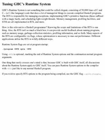
Tuning GHC's Runtime SystemGHC's Runtime System is not something that could be called elegant, consisting of 50,000 lines of C andC-- (a C-like language) code that does a lot of managerial things to execute compiled Haskell programs.The RTS is responsible for managing exceptions, implementing GHC's primitive functions (those suffixedwith a magic hash), and scheduling light-weight threads. Memory management, profiling facilities, andSTM are all implemented in RTS, and more.

How is this relevant to a Haskell programmer? Knowing the scope and limitations of the RTS is onething. Also, the RTS isn't so much a black box; it can provide useful feedback about running programs,such as memory usage, garbage-collection statistics, profiling information, and so forth. Many aspects ofthe RTS are configurable via flags, whose optimization is necessary to max out performance. Differentapplications utilize the RTS in wildly different ways.

Runtime System flags are set at program startup:

./program +RTS opts -RTS

Using -RTS is optional, marking the end of Runtime System options and the continuation normal programarguments.

One thing that rarely crosses one's mind is that, because GHC is built with GHC itself, all discussionsabout the Runtime System apply to GHC itself. You can pass Runtime System options to the compilerwith +RTS just like to any normal Haskell program.

If you wish to specify RTS options to the program being compiled, use the GHC flag --with-rtsopts.

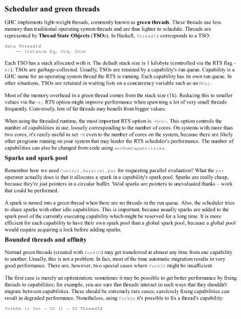
Scheduler and green threadsGHC implements light-weight threads, commonly known as green threads. These threads use lessmemory than traditional operating system threads and are thus lighter to schedule. Threads arerepresented by Thread State Objects (TSOs). In Haskell, ThreadId corresponds to a TSO:

data ThreadId -- instance Eq, Ord, Show

Each TSO has a stack allocated with it. The default stack size is 1 kilobyte (controlled via the RTS flag -ki). TSOs are garbage-collected. Usually, TSOs are retained by a capability's run queue. Capability is aGHC name for an operating system thread the RTS is running. Each capability has its own run queue. Inother situations, TSOs are retained in waiting lists on a concurrency variable such as an MVar.

Most of the memory overhead in a green thread comes from the stack size (1k). Reducing this to smallervalues via the-ki RTS option might improve performance when spawning a lot of very small threadsfrequently. Conversely, lots of fat threads may benefit from bigger values.

When using the threaded runtime, the most important RTS option is -N<n>. This option controls thenumber of capabilities in use, loosely corresponding to the number of cores. On systems with more thantwo cores, it's rarely useful to set -N even to the number of cores on the system, because there are likelyother programs running on your system that may hinder the RTS scheduler's performance. The number ofcapabilities can also be changed from code using setNumCapabilities.

Sparks and spark pool

Remember how we used Control.Parallel.par for requesting parallel evaluation? What the paroperator actually does is that it allocates a spark in a capability's spark pool. Sparks are really cheap,because they're just pointers in a circular buffer. Valid sparks are pointers to unevaluated thunks – workthat could be performed.

A spark is turned into a green thread when there are no threads in the run queue. Also, the scheduler triesto share sparks with other idle capabilities. This is important, because usually sparks are added to thespark pool of the currently executing capability which might be reserved for a long time. It is moreefficient for each capability to have their own spark pool than a global spark pool, because a global poolwould require acquiring a lock before adding sparks.

Bounded threads and affinity

Normal green threads (created with forkIO) may get transferred at almost any time from one capabilityto another. Usually, this is not a problem. In fact, most of the time automatic migration results in verygood performance. There are, however, two special cases where forkIO might be insufficient.

The first case is merely an optimization: sometimes it may be possible to get better performance by fixingthreads to capabilities; for example, you are sure that threads interact in such ways that they shouldn'tmigrate between capabilities. These should be extremely rare cases; carelessly fixing capabilities canresult in degraded performance. Nonetheless, using forkOn it's possible to fix a thread's capability:

forkOn :: Int → IO () → IO ThreadId

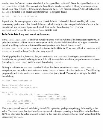
Another case that's more common is related to foreign calls to or from C. Some foreign calls depend onOS-thread-local state. This means that a thread that's interfacing with a C library which depends onthread-local state (OpenGL, for example), should use the forkOS function instead. A thread forked withforkOS is bounded to an operating system thread – a bounded thread:

forkOS :: IO () → IO ThreadId

In particular, the main program is always a bounded thread. Unbounded threads usually yield betterconcurrency performance than bounded threads, which is why it's discouraged to do lots of work in themain thread in a concurrent program. Instead, fork worker threads using forkIO or userunInUnboundThread (a runInBoundThread exists, too).

Indefinite blocking and weak references

The BlockedIndefinitely family of exceptions come with a detail that's not immediately apparent. Inprinciple, a thread will not receive an exception of the blocked indefinitely kind as long as some otherthread is holding a reference that could be used to unblock the thread. In the case ofBlockedIndefinitelyOnMVar, one such reference is the MVar itself; we can unblock a takeMVar witha putMVar in another thread (or the other way around).

The nitty-gritty detail is, however, that just a reference to a ThreadId is enough to prevent blockedindefinitely exceptions from being thrown. After all, we could throw arbitrary asynchronous exceptions(including ThreadKilled) to the blocked thread using throwTo.

To keep a reference to a ThreadId and still allow that thread to receive blocked indefinitelyexceptions, we can make a weak reference to the ThreadId instead of a direct reference. The followingprogram doesn't retain a reference to the ThreadId but just a Weak ThreadId, resulting in the childthread dying:

-- file: weak-threadid.hs

import Control.Concurrentimport Control.Concurrent.MVar

main = do tid <- forkFinally (do { var <- newEmptyMVar ; takeMVar (var :: MVar ()) }) print >>= mkWeakThreadId threadDelay 10000000 print =<< deRefWeak tid

This outputs thread blocked indefinitely in an MVar operation, perhaps surprisingly followed by a Justvalue. The doRefWeak function de-references a weak reference, returning nothing if the value had beenGC'd, or otherwise the value wrapped in Just. In this case, the garbage-collector hadn't yet collected theunnecessary ThreadId.

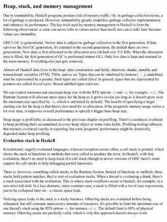
Heap, stack, and memory managementDue to immutability, Haskell programs produce lots of memory traffic. Or, in garbage-collection terms, alot of garbage is produced. However, immutability greatly simplifies garbage collector implementationand enhances its performance. The key trick used by memory management in Haskell is from thefollowing observation: a value can never refer to values newer than itself, nor can it refer later becausevalues are immutable.

GHC's GC is generational. Newer data is subject to garbage collection in the first generation. If datasurvives the first GC generation, it's retained in the second generation. By default there are twogenerations. New data is first allocated in the allocation area (default size 512 KB). When the allocationarea is filled, the first generation of GC is performed (minor GC). Only live data is kept and retained inthe main memory. Everything else just gets removed.

Almost all Haskell data lives in the heap: data constructors and fields, functions, thunks, mutable andtransactional variables (STM), TSOs, and so on. Types that can be inhabited by bottom (_|_), undefined,must be represented by a pointer. Such types are called lifted. In general, types that are represented bypointers are called boxed types. Boxed unlifted types exist too.

We can control minimum and maximum heap size with the RTS options -H and -M, for example,-H1G. TheRuntime System will allocate more space for the heap as it grows in size (as long as it doesn't grow overthe maximum size specified by -M, which is unlimited by default). The benefit of specifying a largerstarting size for the heap is that there's less need for re-allocation. If the program's memory usage varies alot over time, it improves overall performance to specify a bigger base heap size.

Heap usage is profilable, as discussed in the previous chapter on profiling. There's a technical overheadin heap profiling that's accumulated in every heap object as some extra fields. Profiling tooling subtractsthat memory overhead exactly in reporting, but some programs' performance might be drasticallydegraded under heap profiling.

Evaluation stack in Haskell

In traditional, eagerly-evaluated languages, when an exception occurs often, a call stack is printed, whichshows the stack of functions or methods that were called to produce the error. In Haskell, with lazyevaluation, there's no need to keep track of a call stack (though in newer versions of GHC there's somesupport for call stacks to help debugging partial functions).

There is, however, something called stacks in the Runtime System. Instead of functions or methods, thesestacks hold pattern matches; they're sort of evaluation stacks. When a thread is evaluating a thunk, there'sa stack associated with the evaluation. This is where stack overflows occur in Haskell, for example, in anon-strict left-fold. In a less dramatic, more common case, a stack is filled with a lot of case expressions,just to be collapsed later on – a classic space leak.

Noticing space leaks in the stack is a tricky business. Often big stacks are evaluated before beingexhausted, but still consume unnecessary amounts of resources. It's possible to limit the maximum size ofone thread's stack using the RTS option -K, for instance,-K1k. The default limit is 80% of physicalmemory. Often big stacks are perfectly valid, which is why this approach doesn't always work.

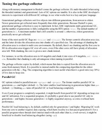
Tuning the garbage collectorAlong with memory management in Haskell comes the garbage collector. It's multi-threaded (when usingthe threaded runtime) and generational. Lots of GC options are tunable. It is also in the GHC developer'sinterests to experiment with different GC settings, to see what works best in a lazy and pure language.

Generational garbage collectors sort live objects into different generations, from newest to oldest.Newer generations get collected more frequently than older generations. Because Haskell is pure,generational garbage collection is easy to implement. In fact, GHC implements multi-generational GC,and the number of generations is fully configurable using the RTS option -G<n>. The default number ofgenerations is 2. A maximum number that's still sensible is around 4; otherwise, oldest generationspractically never get collected.

Some of the most useful GC flags are -A<size> and -n<size>. The former controls allocation area size,and the latter divides the allocation area into chunks of a specified size. The advantage of chunking theallocation area is evident in multi-core environments. By default, there's no chunking and the first core tofill its allocation area triggers GC over all cores, even if the other cores still have plenty of allocationarea left. With chunking, the core is given a new chunk instead.

For instance, to set the allocation area to 64 megabits and chunk it into sizes of 4 megabits, set -A64m -n4m. Remember that chunking is only advantageous when running in parallel.

The garbage collector copies by default, which means that data is copied from the allocation area tosome fresh memory block. It is possible to instead enable the compacting algorithm for the oldestgeneration with the-c flag. The compacting algorithm is most useful when there's a good ratio (say 30%)of live data to heap size.

Parallel GC

GC options related to parallelism are -qg<gen> and -qb<gen>. The former enables parallel GC ingenerations gen and higher (default: 0). The latter enables load-balancing in generations higher than gen(default: 1). Omitting gen turns off parallel GC or load balancing completely.

Even if your program is completely sequential, it might benefit from parallel GC depending on heap sizeand GC utilization. For a sequential program, it's probably a good idea to use parallel GC only ingenerations 1 and higher, because generation 0 is highly sequential anyway, so extra overhead hurtsperformance.

Parallel GC load balancing is, by default, enabled only for generations 1 and higher. Migrating GC workfrom one core to another requires data copying, which hurts locality in a fast-paced generation 0. For aparallel program where threads don't interact much with each other (that is, a web server), it might bebeneficial to disable load balancing altogether (using -qb).

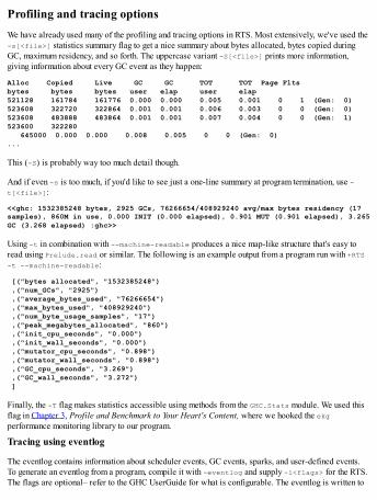
Profiling and tracing optionsWe have already used many of the profiling and tracing options in RTS. Most extensively, we've used the-s[<file>] statistics summary flag to get a nice summary about bytes allocated, bytes copied duringGC, maximum residency, and so forth. The uppercase variant -S[<file>] prints more information,giving information about every GC event as they happen:

Alloc Copied Live GC GC TOT TOT Page Fltsbytes bytes bytes user elap user elap521128 161784 161776 0.000 0.000 0.005 0.001 0 1 (Gen: 0)523608 322720 322864 0.001 0.001 0.006 0.003 0 0 (Gen: 0)523608 483888 483864 0.001 0.001 0.007 0.004 0 0 (Gen: 1)523600 322280 645000 0.000 0.000 0.008 0.005 0 0 (Gen: 0)...

This (-S) is probably way too much detail though.

And if even -s is too much, if you'd like to see just a one-line summary at program termination, use -t[<file>]:

<<ghc: 1532385248 bytes, 2925 GCs, 76266654/408929240 avg/max bytes residency (17 samples), 860M in use, 0.000 INIT (0.000 elapsed), 0.901 MUT (0.901 elapsed), 3.265 GC (3.268 elapsed) :ghc>>

Using -t in combination with --machine-readable produces a nice map-like structure that's easy toread using Prelude.read or similar. The following is an example output from a program run with +RTS-t --machine-readable:

[("bytes allocated", "1532385248") ,("num_GCs", "2925") ,("average_bytes_used", "76266654") ,("max_bytes_used", "408929240") ,("num_byte_usage_samples", "17") ,("peak_megabytes_allocated", "860") ,("init_cpu_seconds", "0.000") ,("init_wall_seconds", "0.000") ,("mutator_cpu_seconds", "0.898") ,("mutator_wall_seconds", "0.898") ,("GC_cpu_seconds", "3.269") ,("GC_wall_seconds", "3.272") ]

Finally, the -T flag makes statistics accessible using methods from the GHC.Stats module. We used thisflag in Chapter 3, Profile and Benchmark to Your Heart's Content, where we hooked the ekgperformance monitoring library to our program.

Tracing using eventlog

The eventlog contains information about scheduler events, GC events, sparks, and user-defined events.To generate an eventlog from a program, compile it with -eventlog and supply -l<flags> for the RTS.The flags are optional– refer to the GHC UserGuide for what is configurable. The eventlog is written to

the program.eventlog file in binary format. The tool that you'll most likely want to inspect the eventlogwith is ThreadScope, as discussed in Chapter 3, Profile and Benchmark to Your Heart's Content.

The eventlog is used for performance profiling. It's possible to emit your own events from code. Usingthe eventlog for event messaging, instead of plain trace debugging, means that the eventlog can showmore information about which processor cores thunks were evaluated or actions performed with. UseDebug.Trace.traceEvent and traceEventIO to emit eventlog events.

Options for profiling and debugging

Profiling and options for profiling have been discussed extensively in Chapter 3, Profile and Benchmarkto Your Heart's Content. Most options require compiling with profiling support, except one, whichgenerates a very basic heap profile in file program.hp: -hT. Use hp2ps to render the report as a nicePostScript graph.

For profiling and debugging multithreaded programs, the RTS clock interval option -V<secs> is ofspecial interest. Setting -V0 effectively makes the scheduler deterministic. The RTS will be doing a lotmore context-switching, but everything is deterministic. Eliminating non-determinism is really useful fordebugging concurrent applications. For instance, determinism ensures reads and writes in concurrentthreads are always performed in the same order.

Summary of useful GHC optionsThe last part of this chapter collects options for GHC and the Runtime System into a concise reference.Let's start off with GHC.

Basic usageThese are some of the most often used general flags related to compilation with GHC:

--make: Compile a multi-module program-j<n>: Parallel compilation-i, -e, runghc: Interactive and evaluation modes-fforce-recomp: Force recompilation-Wall: Turn on all code-level warnings-Werror: Turn all warnings into errors-freverse-errors: Print top-most error last

The LLVM backendThe LLVM route is the preferred compilation path for numeric code. It requires the LLVM libraries and acompatible system. The flags used to enable LLVM are:

-fllvm: Compile via LLVM-optlo-O3: Enable optimizations in the LLVM backend

Turn optimizations on and offGHC has a sophisticated optimization pipeline. Every optimization can be turned on and off separately,but that's rarely necessary. Good default sets of optimizations are enabled with the -O family of flags:

-O: Standard set of benign optimizations (same as -O1)-Odph, -O2, -O3: Enable more optimizations-fno-state-hack: Disable the state hack optimization-ffloat-in, -ffull-laziness: Let-floating in and out-fno-cse: Disable common subexpression elimination (CSE) optimization

Configuring the Runtime System (compile-time)The following flags affect the Runtime System that is linked to the program. The Runtime System hasconfigurable flags of its own, discussed later on:

-threaded: Link with threaded Runtime System-with-rtsopts=<opts>: Specify RTS flags at link time-debug: Enable additional RTS debug events-eventlog: Enable event tracing for ThreadScope-rtsopts={none,some,all}: Enable configuring RTSoptions via ./program +RTS-static, -dynamic: Link Haskell libraries statically or dynamically (default: -static)-shared -fPIC: Build a shared object-optl-static: Link non-Haskell libraries statically

Safe HaskellThese are flags for controlling Safe Haskell compilation:

-XSafe, -XTrustworthy, -XUnsafe: Enable Safe Haskell extensions-fpackage-trust: Refuse compiling untrusted code

Summary of useful RTS optionsThe following sections describe flags for controlling the Runtime System's behavior. The exact set offlags available depend on how the Runtime System was configured (via GHC flags).

Scheduler flagsThe number of capabilities (OS threads) to use is controlled with N<n>:. This can be changed withsetNumCapabilities. (default: 1)

Memory managementThese are flags for controlling used heap and stack size:

-H<size>: Minimum heap size (default: 0)-M<size>: Maximum heap size (default: unlimited)-ki<size>: Minimum stack size (default: 512k)-K<size>: Maximum stack size (default: 80% system memory)

Garbage collectionThese are flags for controlling the generational garbage collector:

-G<n>: Number of GC generations (default: 2)-qg<gen>: Minimum generation to apply parallel GC to (default: 0)-qb<gen>: Minimum generation in parallel GC to apply load-balancing (default: 1)-c: Enable compacting algorithm for oldest generation

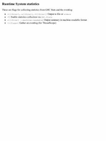
Runtime System statisticsThese are flags for collecting statistics from GHC Stats and the eventlog:

-t[<file>], -s[<file>], -S[<file>]: Output to file or stderr-T: Enable statistics collection via GHC.Stats-t[<file>] --machine-readable: Output summary in machine-readable format-l<flags>: Gather an eventlog (for ThreadScope)

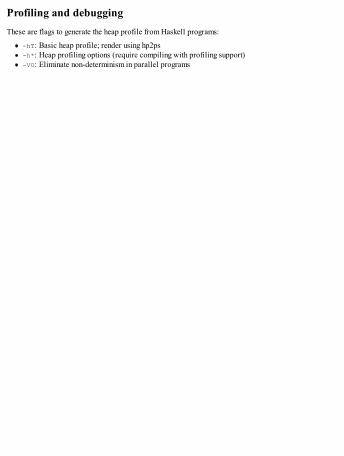
Profiling and debuggingThese are flags to generate the heap profile from Haskell programs:

-hT: Basic heap profile; render using hp2ps-h*: Heap profiling options (require compiling with profiling support)-V0: Eliminate non-determinism in parallel programs

SummaryIn this chapter, we have discussed the easiest way to increase GHC Haskell's performance: tweakingcompiler and Runtime System flags. Enabling optimizations, compiling via LLVM, and enabling LLVMoptimizations is a quick route to a usually very respectable performance. Although most of the timeGHC's sophisticated, heuristic optimizations produce faster code, this is not always the case. Someoptimizations produce slow and even incorrect code under certain situations. Unsafe functions inparticular interact badly with many optimizations. Furthermore, eager inlining may produce very bigbinaries.

We discussed features in the Runtime System and how to enable and configure them. Light-weight (green)threads were cheap, scheduled by RTS, and enabled easy concurrent evaluation via sparks, but werelimited with regard to foreign system calls. The parallel and generational garbage collector also hadmultiple tunable parameters to experiment with.

In the next chapter, we will learn to read GHC's intermediate language, Core. It allows us to observewhether the optimizer did the right thing. For example, unboxing is explicit in Core.

Chapter 9. GHC Internals and Code GenerationIn the previous chapter, we learned to tweak options in GHC and Runtime System. In this chapter, wewill dive into GHC's internal language, Core. We will learn to read Core and to spot possible problemsin Core. Such problems arise when, for instance, the strictness analyzer left an argument lazy and boxed,while it would have been a lot more performant to make it strict and unboxed. We can basically just readsuch situations from Core, because strictness is explicit and unboxed arguments are always output withhashes.

Recall that the hash suffix is referred to as the magic hash in Haskell. Magic hashes mark primitivefunctions and types (those provided by GHC itself). We call these primops. In this chapter, we will learnto program with primops directly. Sometimes raw primop programming is an easy way to get reliablygood performance. Also, a lesser-known fact is that GHC supports some SIMD operations via the LLVMbackend. As of now, SIMD support is not complete and not as powerful as it could be, but still useful at asmall scale. We'll use SIMD as an example of primop programming.

Our third main topic is meta-programming using Template Haskell and datatype generic programmingusing GHC Generics. Generic programming in Haskell is quite pleasant and, what's even better, inprinciple comes with a zero runtime overhead. Template Haskell is really powerful, albeit slightlyverbose. Like, with great power comes great responsibilities, meta-programming should always be thelast resort!

In this chapter, we will cover the following topics:

Making sense of the Core languageProgramming with GHC primitivesUsing GHC Generics to write data-type-generic codeMeta-programming with Template Haskell

Interpreting GHC's internal representationsThe first internal representation in GHC is Core, the second one is STG, and the third one Cmm. BothCore and STG are very functional, while Cmm is an imperative language which resembles C a lot. In thissection we will learn to read GHC Core and to spot possible performance problems that might otherwisebe hard to spot.

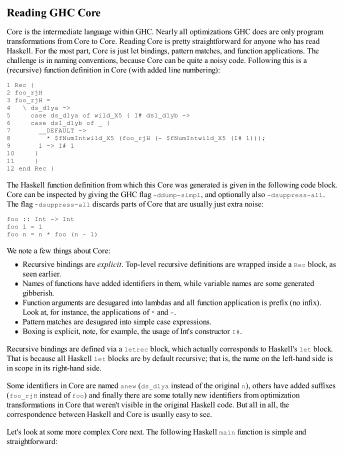
Reading GHC CoreCore is the intermediate language within GHC. Nearly all optimizations GHC does are only programtransformations from Core to Core. Reading Core is pretty straightforward for anyone who has readHaskell. For the most part, Core is just let bindings, pattern matches, and function applications. Thechallenge is in naming conventions, because Core can be quite a noisy code. Following this is a(recursive) function definition in Core (with added line numbering):

1 Rec {2 foo_rjH3 foo_rjH =4 \ ds_d1ya ->5 case ds_d1ya of wild_X5 { I# ds1_d1yb ->6 case ds1_d1yb of _ {7 __DEFAULT ->8 * $fNumIntwild_X5 (foo_rjH (- $fNumIntwild_X5 (I# 1)));9 1 -> I# 110 }11 }12 end Rec }

The Haskell function definition from which this Core was generated is given in the following code block.Core can be inspected by giving the GHC flag -ddump-simpl, and optionally also -dsuppress-all.The flag -dsuppress-all discards parts of Core that are usually just extra noise:

foo :: Int -> Intfoo 1 = 1foo n = n * foo (n – 1)

We note a few things about Core:

Recursive bindings are explicit. Top-level recursive definitions are wrapped inside a Rec block, asseen earlier.Names of functions have added identifiers in them, while variable names are some generatedgibberish.Function arguments are desugared into lambdas and all function application is prefix (no infix).Look at, for instance, the applications of * and -.Pattern matches are desugared into simple case expressions.Boxing is explicit, note, for example, the usage of Int's constructor I#.

Recursive bindings are defined via a letrec block, which actually corresponds to Haskell's let block.That is because all Haskell let blocks are by default recursive; that is, the name on the left-hand side isin scope in its right-hand side.

Some identifiers in Core are named anew (ds_d1ya instead of the original n), others have added suffixes(foo_rjH instead of foo) and finally there are some totally new identifiers from optimizationtransformations in Core that weren't visible in the original Haskell code. But all in all, thecorrespondence between Haskell and Core is usually easy to see.

Let's look at some more complex Core next. The following Haskell main function is simple andstraightforward:

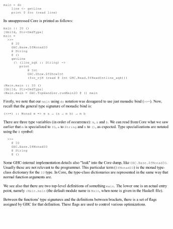
main = do line <- getLine print $ foo (read line)

Its unsuppressed Core is printed as follows:

main :: IO ()[GblId, Str=DmdType]main = >>= @ IO GHC.Base.$fMonadIO @ String @ () getLine (\ (line_aqk :: String) -> print @ Int GHC.Show.$fShowInt (foo_rjH (read @ Int GHC.Read.$fReadIntline_aqk)))

:Main.main :: IO ()[GblId, Str=DmdType]:Main.main = GHC.TopHandler.runMainIO @ () main

Firstly, we note that our main using do notation was desugared to use just monadic bind (>>=). Now,recall that the general type signature of monadic bind is:

(>>=) :: Monad m => m a → (a → m b) → m b

There are three type variables (in order of occurrence): m, a and b. We can read from Core what we sawearlier that m is specialized to IO, a to String and b to (), as expected. Type specializations are notatedusing the @ symbol:

>>= @ IO GHC.Base.$fMonadIO @ String @ ()

Some GHC-internal implementation details also "leak" into the Core dump, like GHC.Base.$fMonadIO.Usually these are not relevant to the programmer. This particular term ($fMonadIO) is the monad type-class dictionary for the IO type. In Core, the type-class dictionaries are represented in the same way thatnormal function arguments are.

We see also that there are two top-level definitions of something main. The lower one is an actual entrypoint, namely :Main.main (the default module name is Main, when none is given in the Haskell file).

Between the functions' type signatures and the definitions between brackets, there is a set of flagsassigned by GHC for that definition. These flags are used to control various optimizations.

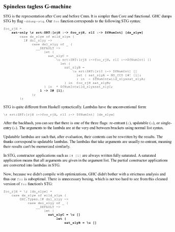
Spineless tagless G-machineSTG is the representation after Core and before Cmm. It is simpler than Core and functional. GHC dumpsSTG by flag -ddump-stg. Our foo function corresponds to the following STG syntax:

foo_rjH = sat-only \r srt:SRT:[rjH :-> foo_rjH, rlI :-> $fNumInt] [ds_s1yw] case ds_s1yw of wild_s1yx { I# ds1_s1yy -> case ds1_s1yy of _ { __DEFAULT -> let { sat_s1yC = \u srt:SRT:[rjH :->foo_rjH, rlI :->$fNumInt] [] let { sat_s1yB = \u srt:SRT:[rlI :-> $fNumInt] [] let { sat_s1yA = NO_CCS I#! [1]; } in - $fNumIntwild_s1yxsat_s1yA; } in foo_rjH sat_s1yB; } in * $fNumIntwild_s1yxsat_s1yC; 1 -> I# [1]; }; };

STG is quite different from Haskell syntactically. Lambdas have the unconventional form:

\r srt:SRT:[rjH :->foo_rjH, rlI :-> $fNumInt] [ds_s1yw]

After the backhash, you can see that there is one of the three flags: re-entrant (r), updatable (u), or single-entry (s). The arguments to the lambda are at the very end between brackets using normal list syntax.

Updatable lambdas are such that, after evaluation, their contents can be rewritten by the results. Thethunks correspond to updatable lambdas. The lambdas that take arguments are usually re-entrant, meaningtheir results can't be memorized similarly.

In STG, constructor applications such as I# [1] are always written fully saturated. A saturatedapplication means that all arguments are given in the argument list. The partial constructor applicationsare converted into lambdas in STG.

Now, because we didn't compile with optimizations, GHC didn't bother with a strictness analysis andthus our foo is suboptimal. There is unnecessary boxing, which is not too hard to see from this cleanedversion of foo function's STG:

foo_rjH = \r [ds_s1yw] = case ds_s1yw of wild_s1yx { GHC.Types.I# ds1_s1yy -> case ds1_s1yy of _ { __DEFAULT -> let { sat_s1yC = \u [] let { sat_s1yB = \u []

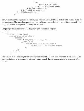
let { sat_s1yA = I#! [1]; } in - wild_s1yxsat_s1yA; } in foo_rjHsat_s1yB; } in * wild_s1yxsat_s1yC; 1 ->GHC.Types.I# [1]; }; };

Here, we can see that arguments to * always get fully evaluated. But GHC pedantically creates thunks forboth arguments. The second argument, sat_s1yC, which corresponds to foo (n-1) is a thunk and so issat_s1yB, which corresponds to the expression (n-1).

Compiling with optimizations (-O) the generated STG is much simpler:

$wfoo = \r srt:SRT:[] [ww_s4wx] case ww_s4wx of ds_s4wy { __DEFAULT -> case -# [ds_s4wy 1] of sat_s4wz { __DEFAULT -> case $wfoosat_s4wz of ww1_s4wA { __DEFAULT -> *# [ds_s4wyww1_s4wA]; }; }; 1 -> 1; };

This version of foo doesn't generate any intermediate thunks. In fact, look at the new name: $wfoo. Thisindicates that foo now operates on unboxed values. Indeed, there is no unwrapping or wrapping of I#values.

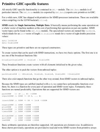
Primitive GHC-specific featuresAll strictly GHC-specific functionality is contained in GHC.* module. The GHC.Exts module is ofparticular interest. The GHC.Prim module (re-exported by GHC.Exts) exports core primitives in GHC.

For a while now, GHC has shipped with primitives for SIMD processor instructions. These are availablewhen compiling via the LLVM backend (-fllvm).

SIMD stands for Single Instruction, Multiple Data. It basically means performing the same operation ona whole vector of machine numbers at the cost of performing that operation on just one number. SIMDvector types can be found in the GHC.Prim module. The specialized vectors are named like Int8X16#,which stands for an Int8 vector of length 16. DoubleX8# stands for a vector of eight double precisionvalues:

data Int8X16#data DoubleX8#

These types are primitive and there are no exposed constructors.

To create vectors that can be used with SIMD instructions, we have two basic options. The first one is touse one of the broadcast functions like:

broadcastDoubleX8# :: Double# → DoubleX8#

These broadcast functions create vectors with all elements initialized to the given value.

The other option is to pack the vectors from unboxed tuples:

packDoubleX4# :: (#Double#, Double#, Double#, Double##) ->DoubleX4#

There also exist unpack functions that go the other way around, from SIMD vectors to unboxed tuples.

Because the SIMD types are unlifted (marked with a #), we cannot have polymorphic functions overthem. So, there is a function for every pair of operation and SIMD vector types. Fortunately, thesefunctions are named predictably. Operations that are supported for SIMD vectors are:

packSXN# :: (# ... #) ->SXN#unpackSXN# :: SXN# -> (# S, ... #)

insertSXN# :: SXN# -> S# -> Int# ->SXN#

negateSXN# :: SXN# ->SXN#plusSXN# :: SXN# ->SXN# ->SXN#minusSXN# :: SXN# ->SXN# ->SXN#timesSXN# :: SXN# ->SXN# ->SXN#

divideSXN# :: SXN# ->SXN# ->SXN#quotSXN# :: SXN# ->SXN# ->SXN#remSXN# :: SXN# ->SXN# ->SXN#

Basic arithmetic operations are therefore supported. All operations are element-wise. In addition tothose shown previously, operations are provided to read and write SIMD vectors from primitive arrays

(ByteArray# and MutableByteArray#) and addresses (Addr#).

The GHC primitive SIMD interface is a bit cumbersome because it is given on top of the primitives.However, if one is desperate to speed up that manual SIMD vectorization, one would usually requiretotal control over strictness and the program flow.

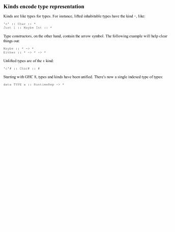
Kinds encode type representationKinds are like types for types. For instance, lifted inhabitable types have the kind *, like:

'c' :: Char :: *Just 1 :: Maybe Int :: *

Type constructors, on the other hand, contain the arrow symbol. The following example will help clearthings out:

Maybe :: * -> *Either :: * -> * -> *

Unlifted types are of the # kind:

'c'# :: Char# :: #

Starting with GHC 8, types and kinds have been unified. There's now a single indexed type of types:

data TYPE a :: RuntimeRep -> *

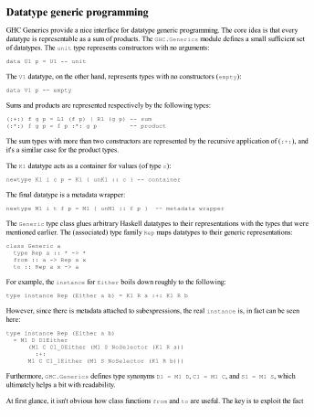
Datatype generic programmingGHC Generics provide a nice interface for datatype generic programming. The core idea is that everydatatype is representable as a sum of products. The GHC.Generics module defines a small sufficient setof datatypes. The unit type represents constructors with no arguments:

data U1 p = U1 -- unit

The V1 datatype, on the other hand, represents types with no constructors (empty):

data V1 p -- empty

Sums and products are represented respectively by the following types:

(:+:) f g p = L1 (f p) | R1 (g p) -- sum(:*:) f g p = f p :*: g p -- product

The sum types with more than two constructors are represented by the recursive application of (:+:), andit's a similar case for the product types.

The K1 datatype acts as a container for values (of type c):

newtype K1 i c p = K1 { unK1 :: c } -- container

The final datatype is a metadata wrapper:

newtype M1 i t f p = M1 { unM1 :: f p } -- metadata wrapper

The Generic type class glues arbitrary Haskell datatypes to their representations with the types that werementioned earlier. The (associated) type family Rep maps datatypes to their generic representations:

class Generic a type Rep a :: * -> * from :: a -> Rep a x to :: Rep a x -> a

For example, the instance for Either boils down roughly to the following:

type instance Rep (Either a b) = K1 R a :+: K1 R b

However, since there is metadata attached to subexpressions, the real instance is, in fact can be seenhere:

type instance Rep (Either a b) = M1 D D1Either (M1 C C1_0Either (M1 S NoSelector (K1 R a)) :+: M1 C C1_1Either (M1 S NoSelector (K1 R b)))

Furthermore, GHC.Generics defines type synonyms D1 = M1 D, C1 = M1 C, and S1 = M1 S, whichultimately helps a bit with readability.

At first glance, it isn't obvious how class functions from and to are useful. The key is to exploit the fact

that these represent something and are supposed to be some constructions of the building blocks—V1, U1,(:*:), (:+:), K1, M1—and nothing else, except some other types wrapped within K1's. This fact nowenables us to create fully datatype generic functions—just overload it over the six generic constructors.

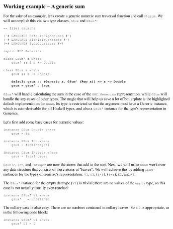
Working example – A generic sumFor the sake of an example, let's create a generic numeric sum traversal function and call it gsum. Wewill accomplish this via two type classes, GSum and GSum':

-- file: gsum.hs

{-# LANGUAGE DefaultSignatures #-}{-# LANGUAGE FlexibleContexts #-}{-# LANGUAGE TypeOperators #-}

import GHC.Generics

class GSum' f where gsum' :: f p -> Double

class GSum a where gsum :: a -> Double

default gsum :: (Generic a, GSum' (Rep a)) => a -> Double gsum = gsum' . from

GSum' will handle calculating the sum in the case of the GHC.Generics representation, while GSum willhandle the any cases of other types. The magic that will help us save a lot of boilerplate is the highlighteddefault implementation for GSum. Its type is restricted so that the argument must have a Generic instance,which is auto-derivable for all Haskell types, and also a GSum' instance for the type's representation inGenerics.

Let's first add some base cases for numeric values:

instance GSum Double where gsum = id

instance GSum Int where gsum = fromIntegral

instance GSum Integer where gsum = fromInteger

Double, Int, and Integer are now the atoms that add to the sum. Next, we will make GSum work overany data structure that consists of these atoms at "leaves". We will achieve this by adding GSum'instances for the types of Generic's representation: V1, U1, (:*:), (:+:), K1, and M1.

The GSum' instance for the empty datatype (V1) is trivial; there are no values of the empty type, so thiscase is not actually usually even reached:

instance GSum' V1 where gsum' _ = undefined

The nullary case is also easy. There are no numbers contained in nullary leaves. So a 0 is appropriate, asin the following code block:

instance GSum' U1 where gsum' U1 = 0

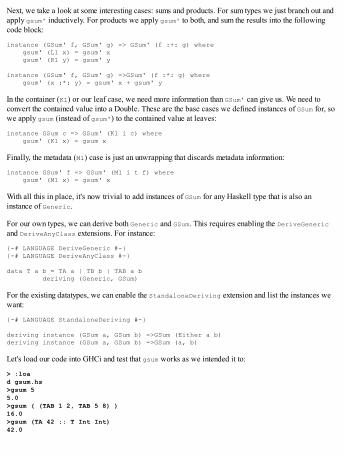
Next, we take a look at some interesting cases: sums and products. For sum types we just branch out andapply gsum' inductively. For products we apply gsum' to both, and sum the results into the followingcode block:

instance (GSum' f, GSum' g) => GSum' (f :+: g) where gsum' (L1 x) = gsum' x gsum' (R1 y) = gsum' y

instance (GSum' f, GSum' g) =>GSum' (f :*: g) where gsum' (x :*: y) = gsum' x + gsum' y

In the container (K1) or our leaf case, we need more information than GSum' can give us. We need toconvert the contained value into a Double. These are the base cases we defined instances of GSum for, sowe apply gsum (instead of gsum') to the contained value at leaves:

instance GSum c => GSum' (K1 i c) where gsum' (K1 x) = gsum x

Finally, the metadata (M1) case is just an unwrapping that discards metadata information:

instance GSum' f => GSum' (M1 i t f) where gsum' (M1 x) = gsum' x

With all this in place, it's now trivial to add instances of GSum for any Haskell type that is also aninstance of Generic.

For our own types, we can derive both Generic and GSum. This requires enabling the DeriveGenericand DeriveAnyClass extensions. For instance:

{-# LANGUAGE DeriveGeneric #-}{-# LANGUAGE DeriveAnyClass #-}

data T a b = TA a | TB b | TAB a b deriving (Generic, GSum)

For the existing datatypes, we can enable the StandaloneDeriving extension and list the instances wewant:

{-# LANGUAGE StandaloneDeriving #-}

deriving instance (GSum a, GSum b) =>GSum (Either a b)deriving instance (GSum a, GSum b) =>GSum (a, b)

Let's load our code into GHCi and test that gsum works as we intended it to:

> :load gsum.hs>gsum 55.0>gsum ( (TAB 1 2, TAB 5 8) )16.0>gsum (TA 42 :: T Int Int)42.0

With quite minimal boilerplate, we managed to create an extendable datatype generic sum function.Everything we did was safe and checked by the type checker at compile time; there was no need for anykind of dynamic typing.

The runtime cost of the GHC Generic representation is 0: there is usually no overhead for GHCGenerics, because the Rep type representation is erased at compile time, unlike the reflection in Java,which has a considerable runtime cost.

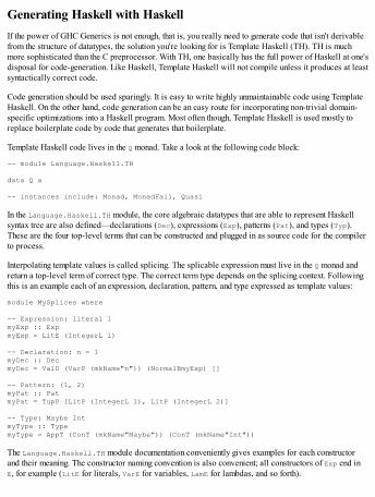
Generating Haskell with HaskellIf the power of GHC Generics is not enough, that is, you really need to generate code that isn't derivablefrom the structure of datatypes, the solution you're looking for is Template Haskell (TH). TH is muchmore sophisticated than the C preprocessor. With TH, one basically has the full power of Haskell at one'sdisposal for code-generation. Like Haskell, Template Haskell will not compile unless it produces at leastsyntactically correct code.

Code generation should be used sparingly. It is easy to write highly unmaintainable code using TemplateHaskell. On the other hand, code generation can be an easy route for incorporating non-trivial domain-specific optimizations into a Haskell program. Most often though, Template Haskell is used mostly toreplace boilerplate code by code that generates that boilerplate.

Template Haskell code lives in the Q monad. Take a look at the following code block:

-- module Language.Haskell.TH

data Q a

-- instances include: Monad, MonadFail, Quasi

In the Language.Haskell.TH module, the core algebraic datatypes that are able to represent Haskellsyntax tree are also defined—declarations (Dec), expressions (Exp), patterns (Pat), and types (Typ).These are the four top-level terms that can be constructed and plugged in as source code for the compilerto process.

Interpolating template values is called splicing. The splicable expression must live in the Q monad andreturn a top-level term of correct type. The correct term type depends on the splicing context. Followingthis is an example each of an expression, declaration, pattern, and type expressed as template values:

module MySplices where

-- Expression: literal 1myExp :: ExpmyExp = LitE (IntegerL 1)

-- Declaration: n = 1myDec :: DecmyDec = ValD (VarP (mkName"n")) (NormalBmyExp) []

-- Pattern: (1, 2)myPat :: PatmyPat = TupP [LitP (IntegerL 1), LitP (IntegerL 2)]

-- Type: Maybe IntmyType :: TypemyType = AppT (ConT (mkName"Maybe")) (ConT (mkName"Int"))

The Language.Haskell.TH module documentation conveniently gives examples for each constructorand their meaning. The constructor naming convention is also convenient; all constructors of Exp end inE, for example (LitE for literals, VarE for variables, LamE for lambdas, and so forth).

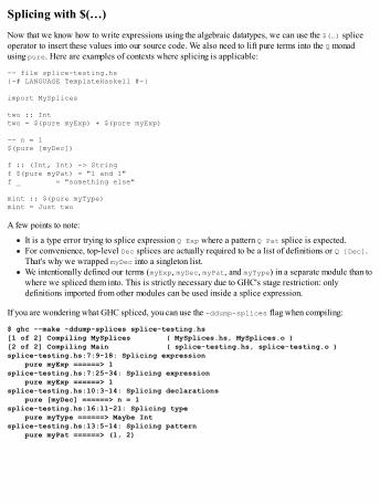
Splicing with $(…)Now that we know how to write expressions using the algebraic datatypes, we can use the $(…) spliceoperator to insert these values into our source code. We also need to lift pure terms into the Q monadusing pure. Here are examples of contexts where splicing is applicable:

-- file splice-testing.hs{-# LANGUAGE TemplateHaskell #-}

import MySplices

two :: Inttwo = $(pure myExp) + $(pure myExp)

-- n = 1$(pure [myDec])

f :: (Int, Int) -> Stringf $(pure myPat) = "1 and 1"f _ = "something else"

mint :: $(pure myType)mint = Just two

A few points to note:

It is a type error trying to splice expression Q Exp where a pattern Q Pat splice is expected.For convenience, top-level Dec splices are actually required to be a list of definitions or Q [Dec].That's why we wrapped myDec into a singleton list.We intentionally defined our terms (myExp, myDec, myPat, and myType) in a separate module than towhere we spliced them into. This is strictly necessary due to GHC's stage restriction: onlydefinitions imported from other modules can be used inside a splice expression.

If you are wondering what GHC spliced, you can use the -ddump-splices flag when compiling:

$ ghc --make -ddump-splices splice-testing.hs[1 of 2] Compiling MySplices ( MySplices.hs, MySplices.o )[2 of 2] Compiling Main ( splice-testing.hs, splice-testing.o )splice-testing.hs:7:9-18: Splicing expression pure myExp ======> 1splice-testing.hs:7:25-34: Splicing expression pure myExp ======> 1splice-testing.hs:10:3-14: Splicing declarations pure [myDec] ======> n = 1splice-testing.hs:16:11-21: Splicing type pure myType ======> Maybe Intsplice-testing.hs:13:5-14: Splicing pattern pure myPat ======> (1, 2)

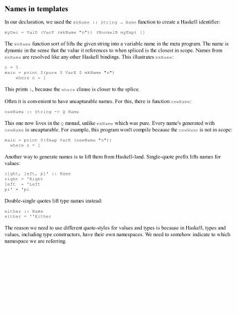
Names in templatesIn our declaration, we used the mkName :: String → Name function to create a Haskell identifier:

myDec = ValD (VarP (mkName "n")) (NormalB myExp) []

The mkName function sort of lifts the given string into a variable name in the meta program. The name isdynamic in the sense that the value it references to when spliced is the closest in scope. Names frommkName are resolved like any other Haskell bindings. This illustrates mkName:

n = 5main = print $(pure $ VarE $ mkName "n") where n = 1

This prints 1, because the where clause is closer to the splice.

Often it is convenient to have uncapturable names. For this, there is function newName:

newName :: String -> Q Name

This one now lives in the Q monad, unlike mkName which was pure. Every name's generated withnewName is uncapturable. For example, this program won't compile because the newName is not in scope:

main = print $(fmap VarE (newName "n")) where n = 1

Another way to generate names is to lift them from Haskell-land. Single-quote prefix lifts names forvalues:

right, left, pi' :: Nameright = 'Rightleft = 'Leftpi' = 'pi

Double-single quotes lift type names instead:

either :: Nameeither = ''Either

The reason we need to use different quote-styles for values and types is because in Haskell, types andvalues, including type constructors, have their own namespaces. We need to somehow indicate to whichnamespace we are referring.

Smart template constructorsFor every datatype constructor (LitE, ValD, and others) there is a "smart" constructor (litE, valD, andothers) whose result and (most) arguments have been lifted to the Q monad. This is often convenient,because sub-expressions don't then need to be explicitly sequenced with monadic bind.

ValD :: Pat -> Body -> [Dec] -> DecvalD :: PatQ -> BodyQ -> [DecQ] -> DecQ

PatQ is just a synonym for Q Pat.

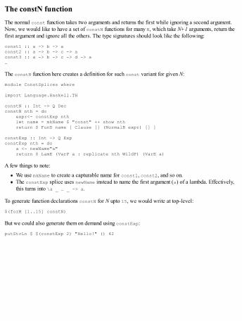
The constN functionThe normal const function takes two arguments and returns the first while ignoring a second argument.Now, we would like to have a set of constN functions for many N, which take N+1 arguments, return thefirst argument and ignore all the others. The type signatures should look like the following:

const1 :: a -> b -> aconst2 :: a -> b -> c -> aconst3 :: a -> b -> c -> d -> a…

The constN function here creates a definition for such const variant for given N:

module ConstSplices where

import Language.Haskell.TH

constN :: Int -> Q DecconstN nth = do expr<- constExp nth let name = mkName $ "const" ++ show nth return $ FunD name [ Clause [] (NormalB expr) [] ]

constExp :: Int -> Q ExpconstExp nth = do a <- newName"a" return $ LamE (VarP a : replicate nth WildP) (VarE a)

A few things to note:

We use mkName to create a capturable name for const1, const2, and so on.The constExp splice uses newName instead to name the first argument (a) of a lambda. Effectively,this turns into \a _ … _ -> a.

To generate function declarations constN for N upto 15, we would write at top-level:

$(forM [1..15] constN)

But we could also generate them on demand using constExp:

putStrLn $ $(constExp 2) "Hello!" () 42

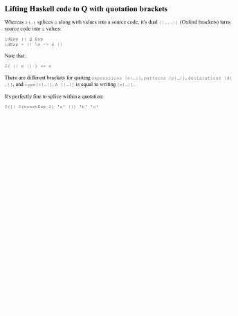
Lifting Haskell code to Q with quotation bracketsWhereas $(…) splices Q along with values into a source code, it's dual [|...|] (Oxford brackets) turnssource code into Q values:

idExp :: Q ExpidExp = [| \x -> x |]

Note that:

$( [| e |] ) == e

There are different brackets for quoting expressions [e|…|], patterns [p|…|], declarations [d|…|], and type[t|…|]. A [|…|] is equal to writing [e|…|].

It's perfectly fine to splice within a quotation:

$([| $(constExp 2) 'a' |]) 'b' 'c'

Launching missiles during compilationIt's possible to embed arbitrary IO actions into the Q monad using runIO:

runIO :: IO a -> Q a

An IO action could be used to embed a compilation timestamp as a constant or to source another file. Forexample, the source for a program written in an embedded domain specific language (DSL) could beread in at compile time and the corresponding Haskell code generated.

Although contrived, you could even read a line from standard input during splicing:

$(fmap (LitE . StringL) $ runIOgetLine)

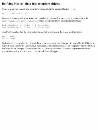
Reifying Haskell data into template objectsGiven a name, we can retrieve some information about the term itself using reify.

reify :: Name -> Q Info

Because type and constructor names may overlap, it is advised to use reify in conjunction withlookupTypeName or lookupValueName which lookup identifiers in correct namespaces:

lookupTypeName :: String -> Q (Maybe Name)lookupValueName :: String -> Q (Maybe Name)

Or, if you're certain that the name is (or should be) in scope, use the single quote notation:

reify 'valuereify ''Type

Reification is very useful, for instance, base code generation on a datatype. It's much like GHC Genericsbut with more flexibility. Common use cases are: defining class instances or completely new boilerplatefunctions for the datatype. For example, the lens library provides TH splices to generate lenses (ageneralization of getters and setters) for user-defined datatypes.

Deriving setters with Template HaskellWhen you declare a record in Haskell, the only way to update one of the fields then is to use the recordsyntax. For instance, we have the following user datatype:

data User = User { firstName :: String , lastName :: String , age :: Int } deriving Show

To update the age field of the user, we would write:

let user' = user { age = newAge }

But if we wanted to, we could write a setter function for a field:

age' :: User -> Int -> Userage' u newAge = u { age = newAge }

let user' = age' user newAge

Writing a setter for every field of every type would be laborious to say the least. Fortunately, we canautomate the process by using a little Template Haskell.

setterDec :: Name -> Q DecsetterDec nm = do let nmD = mkName $ nameBase nm ++ "'"-- (2)

nmV<- newName"val" nmP<- newName"p"

let pat = [VarPnmV, VarPnmP] -- (3) body = NormalB $ RecUpdE (VarEnmP) [ (nm, VarEnmV) ] -- (4)

return $ FunDnmD [ Clause pat body [] ] --(1)

At (1), we build a function definition (FunD) named field' for a given field. The name is specified at(2) using mkName from the field name that is given as an argument to our setterDec template function.Note that a function may have multiple definitions with different patterns, therefore the second argumentto FunD is a list of clauses.

In lines (3) and (4), we have defined arguments to our setter function (new field value and the objectitself). The arguments val and p are given new unique names using newName. The record update itself isencoded in a record update expression using the RecUpdE constructor.

To create setters for every field of a datatype at once, we can write another template function:

deriveSetters :: Name -> Q [Dec]deriveSetters nm = do TyConItyCon<- reify nm -- (1) case tyCon of DataD _ nm tyVarscs _ -> do -- (2) let fieldsTypes = nub (concatMaprecFieldscs) -- (3)

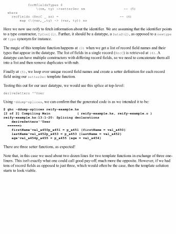
forMfieldsTypes $ \(nm, ty) ->setterDec nm -- (5) where recFields (RecC _ xs) = -- (4) map (\(var,_,ty) -> (var, ty)) xs

Here we now use reify to fetch information about the identifier. We are assuming that the identifier pointsto a type constructor, TyConI(1). Further, it should be a datatype, a DataD(2), as opposed to a newtypeor type synonym for instance.

The magic of this template function happens at (3) when we get a list of record field names and theirtypes that appear in the datatype. The list of fields in a single record (RecC) is retrieved at (4). Adatatype can have multiple constructors with differing record fields, so we need to concatenate them allinto a list and then remove duplicates with nub.

Finally at (5), we loop over unique record field names and create a setter definition for each recordfield using our setterDec template function.

Testing this out for our user datatype, we would use this splice at top-level:

deriveSetters ''User

Using -ddump-splices, we can confirm that the generated code is as we intended it to be:

$ ghc -ddump-splices reify-example.hs[2 of 2] Compiling Main ( reify-example.hs, reify-example.o )reify-example.hs:13:1-20: Splicing declarations deriveSetters''User ======> firstName'val_a450p_a451 = p_a451 {firstName = val_a450} lastName'val_a452p_a453 = p_a453 {lastName = val_a452} age'val_a454p_a455 = p_a455 {age = val_a454}

There are three setter functions, as expected!

Note that, in this case we used about two dozen lines for two template functions in exchange of three one-liners. This isn't exactly what one could call good pay-off; much more the opposite. However, if we hadtens of record fields as opposed to just three, which would often be the case, then the template solutionstarts to look viable.

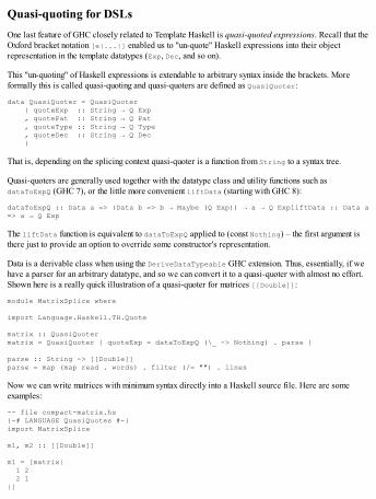
Quasi-quoting for DSLsOne last feature of GHC closely related to Template Haskell is quasi-quoted expressions. Recall that theOxford bracket notation [e|...|] enabled us to "un-quote" Haskell expressions into their objectrepresentation in the template datatypes (Exp, Dec, and so on).

This "un-quoting" of Haskell expressions is extendable to arbitrary syntax inside the brackets. Moreformally this is called quasi-quoting and quasi-quoters are defined as QuasiQuoter:

data QuasiQuoter = QuasiQuoter { quoteExp :: String → Q Exp , quotePat :: String → Q Pat , quoteType :: String → Q Type , quoteDec :: String → Q Dec }

That is, depending on the splicing context quasi-quoter is a function from String to a syntax tree.

Quasi-quoters are generally used together with the datatype class and utility functions such asdataToExpQ (GHC 7), or the little more convenient liftData (starting with GHC 8):

dataToExpQ :: Data a => (Data b => b → Maybe (Q Exp)) → a → Q ExpliftData :: Data a => a → Q Exp

The liftData function is equivalent to dataToExpQ applied to (const Nothing) – the first argument isthere just to provide an option to override some constructor's representation.

Data is a derivable class when using the DeriveDataTypeable GHC extension. Thus, essentially, if wehave a parser for an arbitrary datatype, and so we can convert it to a quasi-quoter with almost no effort.Shown here is a really quick illustration of a quasi-quoter for matrices [[Double]]:

module MatrixSplice where

import Language.Haskell.TH.Quote

matrix :: QuasiQuotermatrix = QuasiQuoter { quoteExp = dataToExpQ (\_ -> Nothing) . parse }

parse :: String -> [[Double]]parse = map (map read . words) . filter (/= "") . lines

Now we can write matrices with minimum syntax directly into a Haskell source file. Here are someexamples:

-- file compact-matrix.hs{-# LANGUAGE QuasiQuotes #-}import MatrixSplice

m1, m2 :: [[Double]]

m1 = [matrix| 1 2 2 1|]

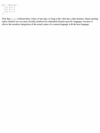
m2 = [matrix| 1.5 4.2 5 5.5 4.1 4 4.5 4 1 6|]

Note that parse could produce values of any type, as long as the value has a data instance. Quasi-quotingmakes Haskell an even more friendly platform for embedded domain-specific languages, because itallows the seamless integration of the actual syntax of a custom language with the host language.

SummaryWe started this chapter from GHC internal representation Core. We looked at the differences in Coresyntax as opposed to Haskell syntax, among them explicit boxing, recursive bindings, explicitspecialization and the passing of class dictionaries. Next, we took a glance at STG, the next internalrepresentation after Core that's even simpler. Then we considered how GHC exposes its primitives:magic hash, unlifted types, and the unlifted kind.

Our second subject was code generation with GHC using GHC Generics. The essential idea withGenerics is to represent every datatype as a sum of products using a handful of indexed datatypes (:+:,:*:, and so on). It then becomes easy to write general functions over all datatypes by converting to orfrom the general sum-of-products representation. Then we looked at full-blown code generation usingTemplate Haskell, which enabled us to generate code, declarations and expressions by directlymanipulating the program's abstract syntax tree.

In the next chapter we will be interacting with other languages from within Haskell, and interacting withHaskell from within other languages. It turns out that Haskell is surprisingly mature in this respect: the Cforeign function interface is very robust and tooling is good. Going the other way around, GHC is able tocompile Haskell into a shared object callable from other languages.

Chapter 10. Foreign Function InterfaceIn the previous chapter, we learned how the GHC code generator works and how to dig deeper into thecompiler pipeline when necessary. In this chapter we will learn to interface with C from Haskell, andwith Haskell functions from C. The foreign function interface (FFI) is part of the Haskell languagereport. The tooling for binding into shared libraries and also for compiling Haskell into shared librariesis quite mature. In this chapter we will cover the fundamentals of the FFI: importing and exportingfunctions, marshalling data, invoking the Haskell runtime from C, and building shared libraries withHaskell.

One of Haskell's strongest points compared to many languages is in fact the FFI: it's relatively easy tointegrate parts written in Haskell to programs written in C or the other way around. By extension,integrating Haskell with other languages by going through the C level is also not too hard. Building ashared library (a shared object or a DLL) with Haskell and GHC is quite easy:

Calling C functions from Haskell and Haskell functions from CUsing Haskell to build a shared library and using the library from CMarshalling pointers and data through the FFI between C and Haskell

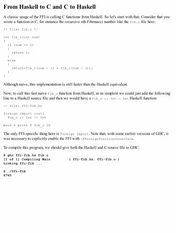
From Haskell to C and C to HaskellA classic usage of the FFI is calling C functions from Haskell. So let's start with that. Consider that youwrote a function in C, for instance the recursive nth Fibonacci number like the fib.c file here:

/* file: fib.c */

int fib_c(int num){ if (num <= 2) { return 1; } else { return(fib_c(num - 1) + fib_c(num - 2)); }}

Although naive, this implementation is still faster than the Haskell equivalent.

Now, to call this fast naive fib_c function from Haskell, at its simplest we could just add the followingline to a Haskell source file and then we would have a fib_c :: Int → Int Haskell function:

-- file: ffi-fib.hs

foreign import ccall fib_c :: Int -> Int

main = print $ fib_c 20

The only FFI-specific thing here is foreign import. Note that, with some earlier versions of GHC, itwas necessary to explicitly enable the FFI with -XForeignFunctionInterface.

To compile this program, we should give both the Haskell and C source file to GHC:

$ ghc ffi-fib.hs fib.c[1 of 1] Compiling Main ( ffi-fib.hs, ffi-fib.o )Linking ffi-fib ...

$ ./ffi-fib6765

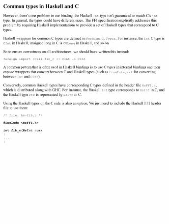
Common types in Haskell and CHowever, there's one problem in our binding: the Haskell Int type isn't guaranteed to match C's inttype. In general, the types could have different sizes. The FFI specification explicitly addresses thisproblem by requiring Haskell implementations to provide a set of Haskell types that correspond to Ctypes.

Haskell wrappers for common C types are defined in Foreign.C.Types. For instance, the int C type isCInt in Haskell, unsigned long in C is CULong in Haskell, and so on.

So to ensure correctness on all architectures, we should have written this instead:

foreign import ccall fib_c :: CInt -> CInt

A common pattern that is often used in Haskell bindings is to use C types in internal bindings and thenexpose wrappers that convert between C and Haskell types (such as fromIntegral for convertingbetween Int and CInt).

Conversely, common Haskell types have corresponding C types defined in the header file HsFFI.h,which is distributed along with GHC. For instance, the Haskell Int type corresponds to HsInt in C, andthe Haskell type Ptr is represented by HsPtr in C.

Using the Haskell types on the C side is also an option. We just need to include the Haskell FFI headerfile to use them:

/* file: hs-fib.c */

#include <HsFFI.h>

int fib_c(HsInt num){...}

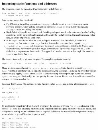
Importing static functions and addressesThe complete syntax for importing C definitions to Haskell-land is:

foreign import <callconv> [safe/unsafe] "<impent>" <variable> :: <type>

Let's see this syntax in more detail:

For C binding, the calling convention <callconv> should be set to ccall, as we did in ourprevious example. Other calling conventions include stdcall for Win32 API bindings, andcplusplus for C++ calling convention.By default foreign calls are marked safe. Marking an import unsafe reduces the overhead of callingan external entity, but unsafe calls cannot call back to the Haskell system. Such callbacks are ratherrare, so unsafe imports are used often.In the impent we define what we wish to import from the C side. If omitted, it defaults to<variable>. For instance, our fib_c function from earlier corresponds to impent "fib_c".<variable> :: <type> just defines how the import looks in Haskell. Note that GHC does zerosanity checking on what you give it as a type. If the Haskell type doesn't align with the C-sidedefinition, a segmentation fault awaits. The types don't need to match exactly though: for instance aBool is a perfectly fine int.

The impent is actually a bit more complex. The complete syntax is given by:

impent → "[static] [chname] [&] [cid]" | "dynamic" | "wrapper"

There are three main alternatives: static, dynamic, or wrapper. Static function import ("static[cid]") is the default behavior. To import a static address, the identifier cid should be preceded with anampersand (&). Typing static in the impent is only necessary when importing C identifiers nameddynamic or wrapper. Optionally, we can specify the exact header file chname from which the identifierto import (cid) is searched for.

Consider this C source file, defining a static function called update and a static address named c_var:

/* file: c_var.c */

int c_var = 0;

void update() { c_var = 42;}

To use these two identifiers from Haskell, we import the variable with type Ptr CInt and update withtype IO (). Note that any static function can be imported either as a pure function or as an IO action. It isleft up to the binding author to choose how to import a definition, because there is no systematic way toknow whether a given C function is pure or not!

-- file: ffi-c-var.hs

import Foreign.C (CInt)import Foreign.Ptr (Ptr)import Foreign.Storable (peek)

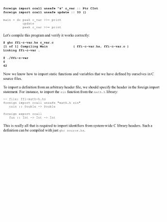
foreign import ccall unsafe "&" c_var :: Ptr CIntforeign import ccall unsafe update :: IO ()

main = do peek c_var >>= print update peek c_var >>= print

Let's compile this program and verify it works correctly:

$ ghc ffi-c-var.hs c_var.c[1 of 1] Compiling Main ( ffi-c-var.hs, ffi-c-var.o )Linking ffi-c-var …

$ ./ffi-c-var042

Now we know how to import static functions and variables that we have defined by ourselves in Csource files.

To import a definition from an arbitrary header file, we should specify the header in the foreign importstatement. For instance, to import the sin function from the math.h library:

-- file: ffi-math-h.hsforeign import ccall unsafe "math.h sin" csin :: Double -> Double

foreign export ccall fun :: Int -> Int -> Int

This is really all that is required to import identifiers from system-wide C library headers. Such adefinition can be compiled with just ghc source.hs.

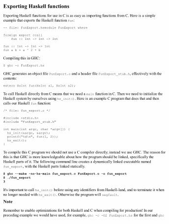
Exporting Haskell functionsExporting Haskell functions for use in C is as easy as importing functions from C. Here is a simpleexample that exports the Haskell function fun:

-- file: FunExport.hsmodule FunExport where

foreign export ccall fun :: Int -> Int -> Int

fun :: Int -> Int -> Intfun a b = a ^ 2 + b

Compiling this in GHC:

$ ghc -c FunExport.hs

GHC generates an object file FunExport.o and a header file FunExport_stub.h, effectively with thecontents:

extern HsInt fun(HsInt a1, HsInt a2);

To call Haskell directly from C means that we need a main function in C. Then we need to initialize theHaskell system by ourselves using hs_init(). Here is an example C program that does that and thencalls our Haskell fun function:

/* file: fun_export.c */

#include <stdio.h>#include "FunExport_stub.h"

int main(int argc, char *argv[]) { hs_init(&argc, &argv); printf("%d\n", fun(1, 2)); hs_exit();}

To compile this C program we should not use a C compiler directly; instead we use GHC. The reason forthis is that GHC is more knowledgeable about how the program should be linked, specifically theHaskell parts of it. The following command line creates a dynamically linked executable namedfun_export, with the Haskell parts linked statically.

$ ghc --make -no-hs-main fun_export.c FunExport.o -o fun_export$ ./fun_export3

It's important to call hs_init() before using any identifiers from Haskell-land, and to terminate it whenno longer needed with hs_exit(). Otherwise the program will segfault.

Note

Remember to enable optimizations for both Haskell and C when compiling for production! In ourpreceding example we would have used, for example, ghc -c -O2 FunExport.hs for the first and ghc

-optc-O … for the C second step.

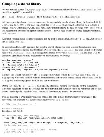
Compiling a shared libraryGiven a Haskell source file, say FunExport.hs, we can create a shared library libfunexport.so withthe following GHC command line:

ghc --make -dynamic -shared -fPIC FunExport.hs -o libfunexport.so

All flags, except perhaps -fPIC, are necessary to successfully build a shared library (at least with GHC7 series and GHC 8.0.1). The most important flag is -shared, which specifies that we want to build ashared library. Unfortunately, GHC does not as yet support building the base libraries with -fPIC, whichis a requirement for embedding into a shared object. Thus we need to link the shared object dynamicallywith -dynamic.

A similar command on a Windows machine can be used to build a DLL instead of a .so file. Just replacethe.so suffix with .dll.

To compile and link a (C) program that uses the shared library, we need to jump through some extrahoops. A complete command line that takes a C source file (fun_export.c) that uses identifiers from theheader file (FunExport_stub.h), links against a shared library (libfunexport.so), and uses GCC tocompile a dynamically linked executable could look like the following:

gcc fun_export.c -o main \-I /usr/lib/ghc-7.10.3/include \-L. -L/usr/lib/ghc-7.10.3/rts \-lHSrts-ghc7.10.3 -lfunexport \-Wl,-rpath=/usr/lib/ghc-7.10.3/rts -Wl,-rpath='$ORIGIN'

The first line is self-explanatory. The -I flag specifies where to find the HsFFI.h header file. The -Lflags specify where the Haskell Runtime System library and our own shared library are located. With the-l flags we are linking against the RTS and our own library.

On the last lines, the -Wl,-rpath=… flags specify additional runtime search paths for the executable.These are necessary so that the libraries can be found when the executable is to be run if they are locatedin non-standard paths. Special $ORIGIN refers to the directory name of the executable.

It's also possible to dynamically load (as opposed to link) a shared library from program code. Thefollowing is an example of a dynamic loading library funexport in C:

/* file: dyn_fun_export.c */

#include <stdio.h>#include <dlfcn.h>

int main(intargc, char *argv[]) { void *dl = dlopen("./libfunexport.so", RTLD_LAZY);

void (*hs_init)(int *argc, char **argv[]) = dlsym(dl, "hs_init"); hs_init(&argc, &argv);

int (*fun)(int a, int b) = dlsym(dl, "fun"); printf("%d\n", fun(1, 2));

}

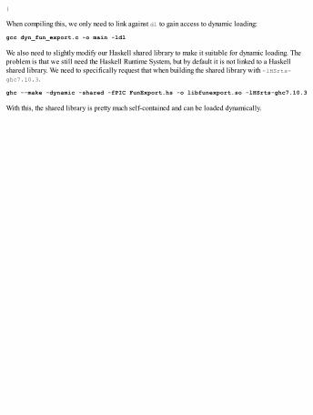
When compiling this, we only need to link against dl to gain access to dynamic loading:

gcc dyn_fun_export.c -o main -ldl

We also need to slightly modify our Haskell shared library to make it suitable for dynamic loading. Theproblem is that we still need the Haskell Runtime System, but by default it is not linked to a Haskellshared library. We need to specifically request that when building the shared library with -lHSrts-ghc7.10.3.

ghc --make -dynamic -shared -fPIC FunExport.hs -o libfunexport.so -lHSrts-ghc7.10.3

With this, the shared library is pretty much self-contained and can be loaded dynamically.

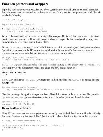
Function pointers and wrappersImporting static functions was easy, but how about dynamic functions and function pointers? In Haskell,function pointers are represented by the datatype FunPtr. To import a function pointer into Haskell-land,we do the following:

-- file: ffi-funptr.hs

import Foreign.Ptr (FunPtr)

foreign import ccall"math.h & cos" p_cos :: FunPtr (Double -> Double)

We need the ampersand and a FunPtr return type. It's also possible for a C function to return a functionpointer, in which case we could leave the ampersand out and import the function statically. In any casethe result is a FunPtr return type in Haskell-land.

To convert a FunPtr return type into a Haskell function to call it, we need to jump through an extra hoop.Specifically, we must ask the FFI to generate a call routine for our specific function type using thedynamic impent. In this case that type is Double -> Double, so we write:

foreign import ccall "dynamic" mkF :: FunPtr (Double -> Double) -> (Double -> Double)

The impent is purely semantic: there is no need to define anything else to generate the call routine. Nowwe can apply mkF to our function pointer and get an ordinary Haskell function:

ghci> (mkF p_cos) pi-1.0

The "dual" of dynamic is wrapper. Wrappers turn Haskell functions into FunPtr to be passed into theforeign side:

foreign import ccall "wrapper" toF :: (Double -> Double) -> IO (FunPtr (Double -> Double))

Note that creating a foreign function pointer from a Haskell function must be an IO action. The types fordynamic and wrapper types must conform to the general formulas (for some Haskell function f):

dynamic: FunPtr f -> fwrapper: f -> IO (FunPtr f)

Haskell callbacks from C

Using FFI wrappers and function pointers we can easily pass Haskell functions as callbacks to foreignfunctions. Consider wanting to call this C function, which takes a function pointer as its first argument:

/* file: callbacks-procedure.c */

void procedure(void (*callback)(double), double n) { callback(n * 3);}

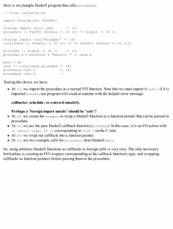
Here is an example Haskell program that calls procedure:

-- file: callbacks.hs

import Foreign.Ptr (FunPtr)

foreign import ccall safe -- (1)procedure :: FunPtr (Double -> IO ()) -> Double -> IO ()

foreign import ccall"wrapper" -- (2)toCallback :: (Double -> IO ()) -> IO (FunPtr (Double -> IO ()))

printRes :: Double -> IO () -- (3)printRes x = putStrLn $ "Result: " ++ show x

main = docont <- toCallback printRes -- (4)procedure cont 5 -- (5)procedure cont 8 --

Tearing this down, we have:

At (1) we import the procedure as a normal FFI function. Note that we must import it safe – if it isimported unsafe, our program will crash at runtime with the helpful error message:

callbacks: schedule: re-entered unsafely.

Perhaps a 'foreign import unsafe' should be 'safe'?At (2) we create the wrapper to wrap a Haskell function as a function pointer that can be passed toprocedure.At (3) we use the pure Haskell callback function (printRes). In this case, it is an I/O action with() result type; IO () corresponding to void * on the C side.At (4) we wrap our callback into a function pointer.At (5) are two example calls for procedure from Haskell main.

So, using arbitrary Haskell functions as callbacks to foreign calls is very easy. The only necessaryboilerplate is creating an FFI wrapper corresponding to the callback function's type, and wrappingcallbacks as function pointers before passing them to the procedure.

Data marshal and stable pointersThe Haskell types Ptr a and FunPtr a represent pointers in foreign, raw memory (outside the Haskellheap). Relevant operations on foreign pointers are provided by the Storable type class, which hasinstances for primitive marshallable data types. A third pointer type is StablePtr a, which is a pointerto an object in the Haskell heap.

On top of passing primitive values and pointers through the FFI, almost arbitrary data can be marshalledbetween Haskell and C (and by extension other languages) relatively easily.

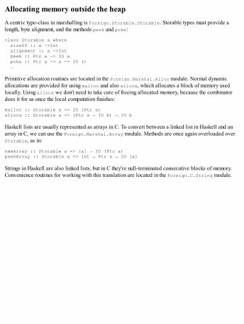
Allocating memory outside the heapA centric type-class in marshalling is Foreign.Storable.Storable. Storable types must provide alength, byte alignment, and the methods peek and poke:

class Storable a where sizeOf :: a ->Int alignment :: a ->Int peek :: Ptr a -> IO a poke :: Ptr a -> a -> IO () …

Primitive allocation routines are located in the Foreign.Marshal.Alloc module. Normal dynamicallocations are provided for using malloc and also alloca, which allocates a block of memory usedlocally. Using alloca we don't need to take care of freeing allocated memory, because the combinatordoes it for us once the local computation finishes:

malloc :: Storable a => IO (Ptr a)alloca :: Storable a => (Ptr a → IO b) → IO b

Haskell lists are usually represented as arrays in C. To convert between a linked list in Haskell and anarray in C, we can use the Foreign.Marshal.Array module. Methods are once again overloaded overStorable, as in:

newArray :: Storable a => [a] → IO (Ptr a)peekArray :: Storable a => Int → Ptr a → IO [a]

Strings in Haskell are also linked lists, but in C they're null-terminated consecutive blocks of memory.Convenience routines for working with this translation are located in the Foreign.C.String module.

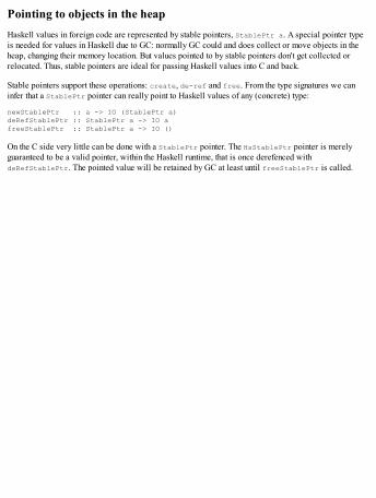
Pointing to objects in the heapHaskell values in foreign code are represented by stable pointers, StablePtr a. A special pointer typeis needed for values in Haskell due to GC: normally GC could and does collect or move objects in theheap, changing their memory location. But values pointed to by stable pointers don't get collected orrelocated. Thus, stable pointers are ideal for passing Haskell values into C and back.

Stable pointers support these operations: create, de-ref and free. From the type signatures we caninfer that a StablePtr pointer can really point to Haskell values of any (concrete) type:

newStablePtr :: a -> IO (StablePtr a)deRefStablePtr :: StablePtr a -> IO afreeStablePtr :: StablePtr a -> IO ()

On the C side very little can be done with a StablePtr pointer. The HsStablePtr pointer is merelyguaranteed to be a valid pointer, within the Haskell runtime, that is once derefenced withdeRefStablePtr. The pointed value will be retained by GC at least until freeStablePtr is called.

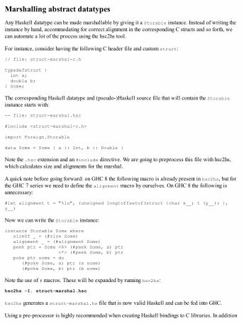
Marshalling abstract datatypesAny Haskell datatype can be made marshallable by giving it a Storable instance. Instead of writing theinstance by hand, accommodating for correct alignment in the corresponding C structs and so forth, wecan automate a lot of the process using the hsc2hs tool.

For instance, consider having the following C header file and custom struct:

// file: struct-marshal-c.h

typedefstruct { int a; double b;} Some;

The corresponding Haskell datatype and (pseudo-)Haskell source file that will contain the Storableinstance starts with:

-- file: struct-marshal.hsc

#include <struct-marshal-c.h>

import Foreign.Storable

data Some = Some { a :: Int, b :: Double }

Note the .hsc extension and an #include directive. We are going to preprocess this file with hsc2hs,which calculates size and alignments for the marshal.

A quick note before going forward: on GHC 8 the following macro is already present in hsc2hs, but forthe GHC 7 series we need to define the alignment macro by ourselves. On GHC 8 the following isunnecessary:

#let alignment t = "%lu", (unsigned long)offsetof(struct {char x__; t (y__); }, y__)

Now we can write the Storable instance:

instance Storable Some where sizeOf _ = (#size Some) alignment _ = (#alignment Some) peek ptr = Some <$> (#peek Some, a) ptr <*> (#peek Some, b) ptr poke ptr some = do (#poke Some, a) ptr (a some) (#poke Some, b) ptr (b some)

Note the use of # macros. These will be expanded by running hsc2hs:

hsc2hs -I. struct-marshal.hsc

hsc2hs generates a struct-marshal.hs file that is now valid Haskell and can be fed into GHC.

Using a pre-processor is highly recommended when creating Haskell bindings to C libraries. In addition

to hsc2hs there is another preprocessor called c2hs. These have many overlapping features but each hassome unique characteristics as well.

Marshalling in standard librariesThe core Haskell container libraries (bytestring, vector, text, and others) include good support forefficient marshalling of their datatypes through the FFI.

All ByteString values are actually already stored outside the Haskell heap, which means that foreigncode can read and write a ByteString with zero copying needed. However, such interoperability isdeemed unsafe because it easily breaks referential transparency. That is why these fast marshallingfunctions are placed in the Data.ByteString.Unsafe module. Slower but safer marshal alternatives arein the Data.ByteString module.

The vector package deals with marshalling by providing custom vector types with storable instances inthe Data.Vector.Storable package. This representation is slightly slower than using pure unboxedvectors, but is the vector type of choice if marshallability is required.

Finally, the text package contains a Data.Text.Foreign module which provides conversion functions.Marshalling unicode-correct text between C is not trivial in every case, so Text marshal is a bit morecomplicated.

SummaryIn this chapter we have imported C functions as Haskell functions, exported Haskell functions as Cfunctions, passed pointers (both foreign and stable) and data through the FFI, built a shared library withHaskell, and used hsc2hsto to write a Storable instance for a custom datatype. You have learned toinvoke the FFI from both the C and the Haskell side and to manage memory in both the Haskell heap andthe lower-level memory area also used by C.

The next chapter will be about another implementation-level concept like the FFI: GPU-programmingusing Haskell. Graphics processors are much better suited for highly parallel number-crunchingapplications, which is the reason for the GPU's popularity in high-performance numeric computing. Anexcellent Haskell library, Accelerate, defines a language that greatly simplifies usually mundane andhard GPU programming. In addition, Accelerate is backend-agnostic: the same code could run on anyhardware solution (CPU/LLVM, CUDA, OpenCL, and others) given a suitable backend implementation.

Chapter 11. Programming for the GPU with AccelerateIn recent years, Graphics Processing Units (GPUs) have become prominent hardware in areas otherthan just plain graphics applications. This practice is known as General-Purpose Computing OnGraphics Processing Units (GPGPU). Due to their ability to perform highly parallel computations muchmore efficiently compared to a CPU, the GPU is often utilized, for instance, in machine-learningapplications. The GPU is specialized to perform certain kinds of vectorized computations extremelyefficiently. It's not nearly as flexible as a CPU is. Single cores in a GPU are far less powerful than CPUcores, but there are hundreds of smaller cores in a GPU.

Due to their parallel nature, GPUs use wildly different instruction sets than, say, the x86. The twodominant ways of writing programs that run on the GPU are Nvidia's proprietary CUDA platform andOpenCL, which is an open source framework and standard for writing programs that run onheterogeneous hardware (CPU, GPU, DSP, FPGA, and others). Both CUDA and OpenCL are designed towork with low-level imperative languages: CUDA for C, C++, and Fortran, while OpenCL defines itsown C-like language.

The Haskell library Accelerate is a high-level EDSL for writing programs that execute on the GPU.Accelerate is fully backend-agnostic: the same Accelerate program can be turned into a CUDAapplication, executed using the reference interpreter on the CPU, and translated into an OpenCLapplication, a Repa application, an LLVM application, or indeed extended with your own backend.Currently, only the interpreter and CUDA backend are considered mature.

In this chapter, we will learn to write high-performance programs with Accelerate and to run them on theGPU. Although first we test our programs using the reference interpreter. The chapter will cover thefollowing topics:

Writing in the core Accelerate language, operations, and expressionsRunning on CUDA and writing efficient high-level GPU programsUsing Accelerate's extra features: tuples, reductions, and backend foreign functions

Writing Accelerate programsAccelerate arrays are indexed by similar data types with Repa arrays, in other words, snoc-style lists:

data Zdata tail :. head = tail :. head

Like Repa, type synonyms are provided for Accelerate indices:

type DIM0 = Ztype DIM1 = DIM0 :. Inttype DIM2 = DIM1 :. Int...

The Accelerate array type is Array sh e. We can build accelerated arrays from lists with fromList:

> import Data.Array.Accelerate as A> fromList (Z :. 5) [1..5]Array (Z :. 5) [1,2,3,4,5]

Now let's try to do something with an Array: reverse it. Accelerate provides the function reverse, but ithas this slightly daunting type signature:

reverse :: Elt e => Acc (Vector e) -> Acc (Vector e)

And if we try to apply reverse to an array directly, we are greeted with a type-mismatch error:

> A.reverse (fromList (Z :. 5) [1..] :: Array DIM1 Int)

<interactive>:24:12: Couldn't match expected type 'Acc (Vector e)' with actual type 'Array DIM1 Int'

The problem is that reverse expects its argument to be a vector wrapped within an acceleratedcomputation: Acc (Vector e). Acc type marks an accelerated computation that produces a value of thegiven type. Vector is just a synonym for a one-dimensional array. Accelerate provides a function to usebare arrays within computations, aptly named use:

use :: Arrays arrays => arrays -> Acc arrays

The reverse function also unsurprisingly returns Acc, an accelerated computation, so we need also someway to run such accelerated computation. One run function is provided by another module:Data.Array.Accelerate.Interpreter. Yet another run is provided by the accelerate-cudapackage, which we'll meet shortly. For now let's use the interpreter:

Data.Array.Accelerate.Interpreter.run :: Arrays a => Acc a → a

The Arrays type-class is used to overload over arrays and tuples of arrays.

Now we have all the pieces needed to reverse an accelerated array, so let's test it out:

>I.run $ A.reverse (use $ fromList (Z :. 5) [1..5]) :: Array DIM1 IntArray (Z :. 5) [5,4,3,2,1]

Kernels – The motivation behind explicit use and runLet's step back and think for a moment. Why did the Accelerate library designers decide that reverseand many other operations should take in and produce arrays inside some Acc context? In theory, the APIcould be completely transparent without exposing the internal Acc context at all.

The reason stems from how the GPU interacts with rest of the computer. The memory of a GPU isseparate from the system RAM. This means that every array and indeed computation we wish to performon the GPU must be loaded into the GPU memory from system memory. Loading stuff into or from theGPU is highly inefficient, so we would like to avoid doing it in excess.

In the lower-level (CUDA and OpenCL) frameworks, we would not only load data (arrays) explicitly butalso define the computing kernels (computations) explicitly. In Accelerate, we load data explicitly butkernel-loading is largely abstracted away. The Acc datatype is in fact a sort of AST that is turned intocode that is then compiled by an Accelerate backend (CUDA, for instance).

The trick that Accelerate employs is that its kernels are created on demand. In addition, for acceptableperformance, it's necessary to memoize often-used kernels so that they're loaded only once. Memoizationis the part where we as library users need to be conscious, because if we write code that doesn't reusekernels enough, it really hurts performance. Arguably, solving this problem perfectly on the library side,even in Haskell, would be akin to solving the halting problem.

The rule of thumb for performance would be to always pass changing arguments inside acceleratedarrays (Acc). Accelerate also provides some debugging tools to diagnose kernel-sharing problems. Butfor now we won't delve into optimizations and instead use Accelerate for getting things done.

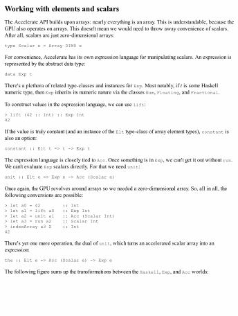
Working with elements and scalarsThe Accelerate API builds upon arrays: nearly everything is an array. This is understandable, because theGPU also operates on arrays. This doesn't mean we would need to throw away convenience of scalars.After all, scalars are just zero-dimensional arrays:

type Scalar e = Array DIM0 e

For convenience, Accelerate has its own expression language for manipulating scalars. An expression isrepresented by the abstract data type:

data Exp t

There's a plethora of related type-classes and instances for Exp. Most notably, if t is some Haskellnumeric type, then Exp inherits its numeric nature via the classes Num, Floating, and Fractional.

To construct values in the expression language, we can use lift:

> lift (42 :: Int) :: Exp Int42

If the value is truly constant (and an instance of the Elt type-class of array element types), constant isalso an option:

constant :: Elt t => t -> Exp t

The expression language is closely tied to Acc. Once something is in Exp, we can't get it out without run.We can't evaluate Exp scalars directly. For that we need unit:

unit :: Elt e => Exp e -> Acc (Scalar e)

Once again, the GPU revolves around arrays so we needed a zero-dimensional array. So, all in all, thefollowing conversions are possible:

> let a0 = 42 :: Int> let a1 = lift a0 :: Exp Int> let a2 = unit a1 :: Acc (Scalar Int)> let a3 = run a2 :: Scalar Int> indexArray a3 Z :: Int42

There's yet one more operation, the dual of unit, which turns an accelerated scalar array into anexpression:

the :: Elt e => Acc (Scalar e) -> Exp e

The following figure sums up the transformations between the Haskell, Exp, and Acc worlds:

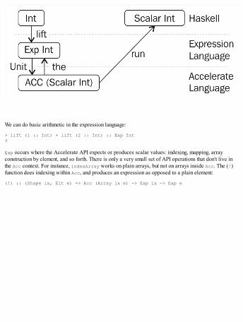
We can do basic arithmetic in the expression language:

> lift (1 :: Int) + lift (2 :: Int) :: Exp Int3

Exp occurs where the Accelerate API expects or produces scalar values: indexing, mapping, arrayconstruction by element, and so forth. There is only a very small set of API operations that don't live inthe Acc context. For instance, indexArray works on plain arrays, but not on arrays inside Acc. The (!)function does indexing within Acc, and produces an expression as opposed to a plain element:

(!) :: (Shape ix, Elt e) => Acc (Array ix e) -> Exp ix -> Exp e

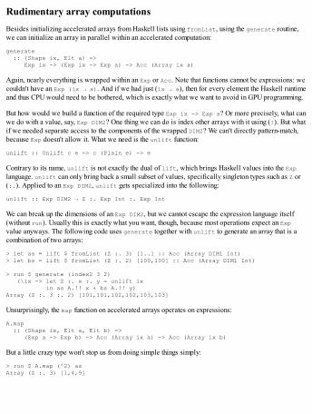
Rudimentary array computationsBesides initializing accelerated arrays from Haskell lists using fromList, using the generate routine,we can initialize an array in parallel within an accelerated computation:

generate :: (Shape ix, Elt a) => Exp ix -> (Exp ix -> Exp a) -> Acc (Array ix a)

Again, nearly everything is wrapped within an Exp or Acc. Note that functions cannot be expressions: wecouldn't have an Exp (ix → a). And if we had just (ix → a), then for every element the Haskell runtimeand thus CPU would need to be bothered, which is exactly what we want to avoid in GPU programming.

But how would we build a function of the required type Exp ix -> Exp a? Or more precisely, what canwe do with a value, say, Exp DIM2? One thing we can do is index other arrays with it using (!). But whatif we needed separate access to the components of the wrapped DIM2? We can't directly pattern-match,because Exp doesn't allow it. What we need is the unlift function:

unlift :: Unlift c e => c (Plain e) -> e

Contrary to its name, unlift is not exactly the dual of lift, which brings Haskell values into the Explanguage. unlift can only bring back a small subset of values, specifically singleton types such as Z or(:.). Applied to an Exp DIM2, unlift gets specialized into the following:

unlift :: Exp DIM2 → Z :. Exp Int :. Exp Int

We can break up the dimensions of an Exp DIM2, but we cannot escape the expression language itself(without run). Usually this is exactly what you want, though, because most operations expect an Expvalue anyways. The following code uses generate together with unlift to generate an array that is acombination of two arrays:

> let as = lift $ fromList (Z :. 3) [1..] :: Acc (Array DIM1 Int)> let bs = lift $ fromList (Z :. 2) [100,100] :: Acc (Array DIM1 Int)

> run $ generate (index2 3 2) (\ix -> let Z :. x :. y = unlift ix in as A.!! x + bs A.!! y)Array (Z :. 3 :. 2) [101,101,102,102,103,103]

Unsurprisingly, the map function on accelerated arrays operates on expressions:

A.map :: (Shape ix, Elt a, Elt b) => (Exp a -> Exp b) -> Acc (Array ix a) -> Acc (Array ix b)

But a little crazy type won't stop us from doing simple things simply:

> run $ A.map (^2) asArray (Z :. 3) [1,4,9]

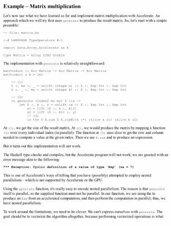
Example – Matrix multiplicationLet's now use what we have learned so far and implement matrix multiplication with Accelerate. Anapproach which we will try first uses generate to produce the result matrix. So, let's start with a simplepreamble:

-- file: matrix.hs

{-# LANGUAGE TypeOperators #-}

import Data.Array.Accelerate as A

type Matrix = Array DIM2 Double

The implementation with generate is relatively straightforward:

matProduct :: Acc Matrix -> Acc Matrix -> Acc MatrixmatProduct a b = let

-- (1) Z :. mx :. _ = unlift (shape a) :: Z :. Exp Int :. Exp Int Z :. _ :. my = unlift (shape b) :: Z :. Exp Int :. Exp Int

-- (2) in generate (index2 mx my) $ \ix -> let Z :. x :. y = unlift ix :: Z :. Exp Int :. Exp Int s1 = lift (Z :. x :. All) s2 = lift (Z :. All :. y) -- (3) in the $ A.sum $ A.zipWith (*) (slice a s1) (slice b s2)

At (1), we get the size of the result matrix. At (2), we would produce the matrix by mapping a function(3) over every individual index (in parallel). The function at (3) uses slice to get the row and columnneeded to compute a value at the given index. Then we use A.sum and to produce an expression.

But it turns out this implementation will not work.

The Haskell type-checks and compiles, but the Accelerate program will not work; we are greeted with anerror message akin to the following:

*** Exception: Cyclic definition of a value of type 'Exp' (sa = 7)

This is one of Accelerate's ways of telling that you have (possibly) attempted to employ nestedparallelism – which is not supported by Accelerate or the GPU.

Using the generate function, it's really easy to encode nested parallelism. The reason is that generateitself is parallel, so the supplied function must not be parallel. In our function, we are using the toproduce an Exp from an accelerated computation, and then perform the computation in parallel; thus, wehave nested parallelism.

To work around the limitations, we need to be clever. We can't express ourselves with generate. Thegoal should be to vectorize the algorithm altogether, because performing vectorized operations is what

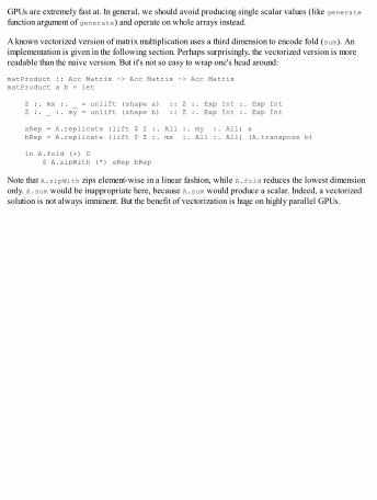
GPUs are extremely fast at. In general, we should avoid producing single scalar values (like generatefunction argument of generate) and operate on whole arrays instead.

A known vectorized version of matrix multiplication uses a third dimension to encode fold (sum). Animplementation is given in the following section. Perhaps surprisingly, the vectorized version is morereadable than the naive version. But it's not so easy to wrap one's head around:

matProduct :: Acc Matrix -> Acc Matrix -> Acc MatrixmatProduct a b = let

Z :. mx :. _ = unlift (shape a) :: Z :. Exp Int :. Exp Int Z :. _ :. my = unlift (shape b) :: Z :. Exp Int :. Exp Int

aRep = A.replicate (lift $ Z :. All :. my :. All) a bRep = A.replicate (lift $ Z :. mx :. All :. All) (A.transpose b)

in A.fold (+) 0 $ A.zipWith (*) aRep bRep

Note that A.zipWith zips element-wise in a linear fashion, while A.fold reduces the lowest dimensiononly. A.sum would be inappropriate here, because A.sum would produce a scalar. Indeed, a vectorizedsolution is not always imminent. But the benefit of vectorization is huge on highly parallel GPUs.

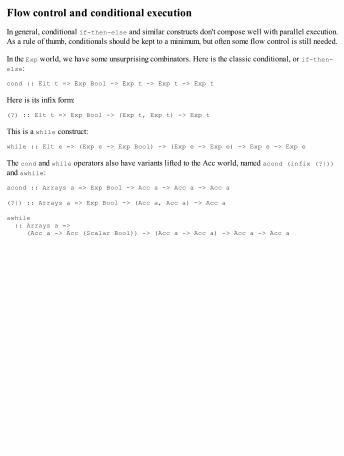
Flow control and conditional executionIn general, conditional if-then-else and similar constructs don't compose well with parallel execution.As a rule of thumb, conditionals should be kept to a minimum, but often some flow control is still needed.

In the Exp world, we have some unsurprising combinators. Here is the classic conditional, or if-then-else:

cond :: Elt t => Exp Bool -> Exp t -> Exp t -> Exp t

Here is its infix form:

(?) :: Elt t => Exp Bool -> (Exp t, Exp t) -> Exp t

This is a while construct:

while :: Elt e => (Exp e -> Exp Bool) -> (Exp e -> Exp e) -> Exp e -> Exp e

The cond and while operators also have variants lifted to the Acc world, named acond (infix (?|))and awhile:

acond :: Arrays a => Exp Bool -> Acc a -> Acc a -> Acc a

(?|) :: Arrays a => Exp Bool -> (Acc a, Acc a) -> Acc a

awhile :: Arrays a => (Acc a -> Acc (Scalar Bool)) -> (Acc a -> Acc a) -> Acc a -> Acc a

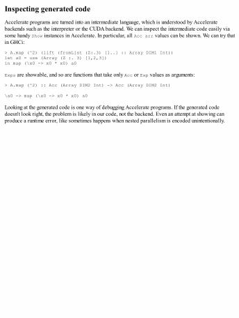
Inspecting generated codeAccelerate programs are turned into an intermediate language, which is understood by Acceleratebackends such as the interpreter or the CUDA backend. We can inspect the intermediate code easily viasome handy Show instances in Accelerate. In particular, all Acc arr values can be shown. We can try thatin GHCi:

> A.map (^2) (lift (fromList (Z:.3) [1..] :: Array DIM1 Int))let a0 = use (Array (Z :. 3) [1,2,3])in map (\x0 -> x0 * x0) a0

Exps are showable, and so are functions that take only Acc or Exp values as arguments:

> A.map (^2) :: Acc (Array DIM2 Int) -> Acc (Array DIM2 Int)

\a0 -> map (\x0 -> x0 * x0) a0

Looking at the generated code is one way of debugging Accelerate programs. If the generated codedoesn't look right, the problem is likely in our code, not the backend. Even an attempt at showing canproduce a runtime error, like sometimes happens when nested parallelism is encoded unintentionally.

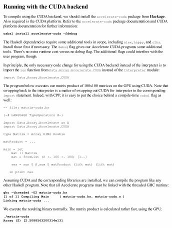
Running with the CUDA backendTo compile using the CUDA backend, we should install the accelerate-cuda package from Hackage.Also required is the CUDA platform. Refer to the accelerate-cuda package documentation and CUDAplatform documentation for further information:

cabal install accelerate-cuda -fdebug

The Haskell dependencies require some additional tools in scope, including alex, happy, and c2hs.Install those first if necessary. The debug flag gives our Accelerate CUDA programs some additionaltools. There's no extra runtime cost versus no debug flag. The additional flags could interfere with theuser program, though.

In principle, the only necessary code change for using the CUDA backend instead of the interpreter is toimport the run function from Data.Array.Accelerate.CUDA instead of the Interpreter module:

import Data.Array.Accelerate.CUDA

The program below executes our matrix product of 100x100 matrices on the GPU using CUDA. Note thatswapping back to the interpreter is a matter of swapping out CUDA for interpreter in the correspondingimport statement. Indeed, with CPP, it is easy to put the choice behind a compile-time cabal flag aswell:

-- file: matrix-cuda.hs

{-# LANGUAGE TypeOperators #-}

import Data.Array.Accelerate as Aimport Data.Array.Accelerate.CUDA

type Matrix = Array DIM2 Double

matProduct = ...

main = let mat :: Matrix mat = fromList (Z :. 100 :. 100) [1..]

res = run $ A.sum $ matProduct (lift mat) (lift mat)

in print res

Assuming CUDA and the corresponding libraries are installed, we can compile the program like anyother Haskell program. Note that all Accelerate programs must be linked with the threaded GHC runtime:

ghc -threaded -O2 matrix-cuda.hs[1 of 1] Compiling Main ( matrix-cuda.hs, matrix-cuda.o )Linking matrix-cuda ...

We execute the resulting binary normally. The matrix product is calculated rather fast, using the GPU:

./matrix-cudaArray (Z) [2.5088563200314e13]

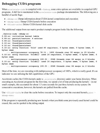
Debugging CUDA programsWhen accelerate-cuda is compiled with -fdebug, some extra options are available in compiled GPUprograms. A full list is maintained in the accelerate-cuda package documentation. The following are ahandful of useful flags:

-ddump-cc: Dump information about CUDA kernel compilation and execution-ddump-exec: Dump CUDA kernels before execution-fflush-cache: Delete CUDA kernel disk cache

The additional output from our matrix product example program looks like the following:

./matrix-cuda -ddump-cc0.09:cc: initialise kernel table0.09:cc: persist/restore: 4 entries0.09:cc: found/persistent0.10:cc: found/persistent0.10:cc: found/persistent0.10:cc: entry function 'fold' used 40 registers, 0 bytes smem, 0 bytes lmem, 0 bytes cmem ... multiprocessor occupancy 78.1% : 1600 threads over 50 warps in 25 blocks0.10:cc: entry function 'foldAll' used 16 registers, 0 bytes smem, 0 bytes lmem, 0 bytes cmem ... multiprocessor occupancy 100.0% : 2048 threads over 64 warps in 2 blocks0.10:cc: entry function 'foldAll' used 16 registers, 0 bytes smem, 0 bytes lmem, 0 bytes cmem ... multiprocessor occupancy 100.0% : 2048 threads over 64 warps in 2 blocks

Most of the time, we are executing with multiprocessor occupancy of 100%, which is really good. It's anindicator we are utilizing the full capabilities of the GPU.

Accelerate caches the CUDA kernels under a .accelerate directory under your home directory. Whenexecuting an Accelerate program for the first time, we spend a lot of time producing the kernels – in oursmall example, this accounted for about 1.5 extra seconds for just three kernels on my system. Onconsecutive executions, however, the kernels are pulled from the cache.

Use -fflush-cache to clear the cache before execution. To inspect only the executed kernels, pass -ddump-exec.

If the program is repeatedly producing new kernels when you think some previously used kernel could bereused, this can be spotted in the debug output.

More Accelerate conceptsSo far, we have considered accelerated arrays and expressions. These are the primitives that Acceleratebuilds upon. On top, we have a bunch of functional machinery to help us express ourselves in acceleratedcomputations: zips and unzips, reductions, permutations, stencils, and so forth. The complete API isdocumented in the accelerate package. In this section, we consider using some of the most useful parts ofthis machinery.

Working with tuplesGPUs don't allow array nesting or tuples as elements of an array. Nested arrays can be somewhatmimicked with higher-dimensional arrays. And it might not come as a surprise that Accelerate supportstuples as elements of an array. Internally, arrays with tupled elements are represented as tuples of arrays,but this is strictly an implementation detail. For the programmer, it really looks like we are working withtupled elements, which is sometimes very convenient.

With zip and unzip, we can (de)construct tupled elements within accelerated arrays with zero runtimecost. A tuple array could be used to represent an array of imaginary numbers, or instances.

The lift and unlift functions translate between tuple expressions and tuples of expressions. Forinstance, these are valid type specializations of lift and unlift:

lift :: (Exp Int, Exp Int) -> Exp (Int, Int)unlift :: Exp (Int, Int) -> (Exp Int, Exp Int)

lift and unlift work with Acc in place of Exp too.

Regarding performance, it doesn't matter whether there is a tuple of expressions (Exp) or an expressionof tuples. They have pretty much the same internal representation and will produce the same program.

Folding, reducing, and segmentingAccelerate provides familiarly named fold and fold1, but unlike those versions of these functions inData.List, the Accelerate ones fold over the innermost dimension only, so they can be used to reducethe rank of an array by one. To fold along all dimensions producing a scalar, functions like foldAll andfold1All can be used.

What's different versus Data.List style folds is that Accelerate's folds always proceed in parallel. Thismeans that the folding function must be associative. To do sequential fold with Accelerate, we wouldneed to use sfoldl, also from the Accelerate library. Note that slfold only reduces along theinnermost slice:

sfoldl :: _ => (Exp a → Exp b → a) → Exp a → Exp sh → Acc (Array (sh :. Int) b) → Exp a

The slice is specified by an argument of type Exp sh. There is no ready-made solution for folding over awhole dimension or all dimensions sequentially. It is not a common need to fold a multi-dimensionalarray non-associatively, and a sequential fold of a big array isn't very efficient on a GPU due to the lackof parallelism.

One more folding variant provided by Accelerate operates on segments:

type Segments i = Vector i

Segments are how nested one-dimensional arrays can be represented in Accelerate: a segment arraygives the lengths of successive logical sub-arrays within an array. The foldSeg and fold1Seg functionsfold over each logical sub-array, producing an array with the same dimensionality but with the logicalsub-arrays reduced.

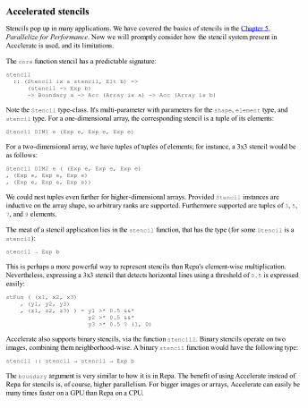
Accelerated stencilsStencils pop up in many applications. We have covered the basics of stencils in the Chapter 5,Parallelize for Performance. Now we will promptly consider how the stencil system present inAccelerate is used, and its limitations.

The core function stencil has a predictable signature:

stencil :: (Stencil ix a stencil, Elt b) => (stencil -> Exp b) -> Boundary a -> Acc (Array ix a) -> Acc (Array ix b)

Note the Stencil type-class. It's multi-parameter with parameters for the shape, element type, andstencil type. For a one-dimensional array, the corresponding stencil is a tuple of its elements:

Stencil DIM1 e (Exp e, Exp e, Exp e)

For a two-dimensional array, we have tuples of tuples of elements; for instance, a 3x3 stencil would beas follows:

Stencil DIM2 e ( (Exp e, Exp e, Exp e), (Exp e, Exp e, Exp e), (Exp e, Exp e, Exp e))

We could nest tuples even further for higher-dimensional arrays. Provided Stencil instances areinductive on the array shape, so arbitrary ranks are supported. Furthermore supported are tuples of 3, 5,7, and 9 elements.

The meat of a stencil application lies in the stencil function, that has the type (for some Stencil is astencil):

stencil → Exp b

This is perhaps a more powerful way to represent stencils than Repa's element-wise multiplication.Nevertheless, expressing a 3x3 stencil that detects horizontal lines using a threshold of 0.5 is expressedeasily:

stFun ( (x1, x2, x3) , (y1, y2, y3) , (z1, z2, z3) ) = y1 >* 0.5 &&* y2 >* 0.5 &&* y3 >* 0.5 ? (1, 0)

Accelerate also supports binary stencils, via the function stencil2. Binary stencils operate on twoimages, combining them neighborhood-wise. A binary stencil function would have the following type:

stencil :: stencil → stencil → Exp b

The boundary argument is very similar to how it is in Repa. The benefit of using Accelerate instead ofRepa for stencils is, of course, higher parallelism. For bigger images or arrays, Accelerate can easily bemany times faster on a GPU than Repa on a CPU.

Permutations in AccelerateA permutation is an array transformation which reorders the elements, possibly replacing some with newelements and maybe altering the shape. Accelerate provides combinators for both forward and backwardpermutations. In a forward permutation, indices are mapped from the input array to the output array.Going backward, output array indices define input indices.

Reverse and transpose are examples of permutations. These two are provided by Accelerate by default.Generic forward permutation is called permute while backward permutation is backpermute.

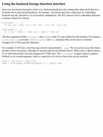
Using the backend foreign function interfaceNot every Accelerate backend is built even. Some backends provide routines that others don't that are alot faster due to specialized hardware, for instance. Accelerate provides a thin layer for embeddingbackend-specific alternatives in accelerated computations. The FFI consists of two embedding functions(contexts omitted for clarity):

foreignAcc :: _ => ff acc res → (Acc acc → Acc res) → Acc acc → Acc res

foreignExp :: _=> ff e res → (Exp e → Exp res) → Exp e → Exp res

The first argument in both foreignAcc and Exp is a value of a type defined by the backend. For instance,accelerate-cuda provides CUDAForeignAcc and *Exp datatypes that can be used to constructwrappers for CUDA-specific functions.

For example, CUDA has a fast float-specialized exponentiation __expf. We can easily access this fasterprimitive from Accelerate, although it's not provided by the Haskell library. What's nice is that by doingso we don't necessarily lock our program for CUDA only. The foreignExp wrapper expects a genericfallback as its second argument, which is expected to be slower, but works on any backend:

fexp :: Exp Float → Exp Floatfexp = foreignExp (CUDAForeignExp [] "__expf") exp

SummaryNow we have learned to write programs with Accelerate that run using the interpreter, and to compileand run them on CUDA-enabled GPUs. We know that Accelerate uses a code generator of its owninternally. We understand it's crucial to write code that can efficiently reuse cached CUDA kernels,because their compilation is very expensive. We also learned that tuples are a free abstraction inAccelerate, although GPUs themselves don't directly support tupled elements.

In the next chapter, we will dive into Cloud Haskell and distributed programming using Haskell. It turnsout Haskell is a pretty well-suited language for programming distributed systems. Cloud Haskell is aneffort that streamlines building distributed applications, providing an abstraction over the network layer,among other things.

Chapter 12. Scaling to the Cloud with Cloud HaskellIn this chapter, we will look at how distributed systems programming fits with Haskell. The motivationbehind distributed systems is multifaceted. On one end, there is more computing power available withmultiple physical machines. Then there are other resources besides computing power: storage space,network bandwidth, and other devices. Yet another advantage of proper distributed systems is resilience.With a growing number of machines, there are a growing number of failure points. A proper distributedsystem should be able to operate under arbitrary process failures.

Cloud Haskell is a relatively new but mature platform that's modelled from Erlang's wonderful executionmodel. Cloud Haskell brings distributed processes and process management to Haskell with modularnetwork transport and fine-grained message and channel-based communication.

In this chapter, we will explore the Cloud Haskell platform. No deep knowledge about distributedsystems is required. A general notion of a distributed system is enough. We will do basic message-passing, work with typed channels, and send and receive both data and closures of arbitrary data,including functions and procedures. We will look at the facilities for handling distributed failure in CloudHaskell, that is, linking and monitoring processes. By the end of this chapter, you will be able to useCloud Haskell to build your distributed system.

The chapter will cover the following topics:

Launching Cloud Haskell nodes and processesMessage-passing and typed channelsUsing closures to pass arbitrary data between machinesHandling failure, linking processes together, and process monitoring

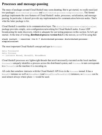
Processes and message-passingThe maze of packages around Cloud Haskell may seem daunting. But to get started, we really need justtwo packages: distributed-process and distributed-process-simplelocalnet. The formerpackage implements the core features of Cloud Haskell: nodes, processes, serialization, and message-passing. In particular, it doesn't provide any implementation for communication between nodes. That'swhat the latter package is for.

Cloud Haskell is modular in its communication layer. The distributed-process-simplelocalnetpackage provides simple, zero-configuration networking for Cloud Haskell nodes. It uses UDPbroadcasting for node discovery, which is adequate for our testing purposes in this section. So let's getstarted. At the time of writing, distributed-process version 0.6.4 is the newest, so we'll be using that:

stack install --resolver lts-6.7 distributed-process distributed-process-simplelocalnet

The most important Cloud Haskell concept and type is Process:

data ProcessIddata Process-- instance Monad, MonadIO, MonadMask

Cloud Haskell processes are lightweight threads that aren't necessarily executed on the local machine.ProcessId uniquely identifies a process across the distributed system, and Process in turn correspondsto a ThreadId on the machine it is executing on.

All code that somehow interacts with the Cloud Haskell API lives in the Process monad. It has aMonadIO instance as well as MonadMask (and MonadThrow/MonadCatch) instances, so Process can beused almost always where plain IO would be used.

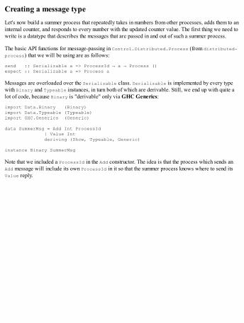
Creating a message typeLet's now build a summer process that repeatedly takes in numbers from other processes, adds them to aninternal counter, and responds to every number with the updated counter value. The first thing we need towrite is a datatype that describes the messages that are passed in and out of such a summer process.

The basic API functions for message-passing in Control.Distributed.Process (from distributed-process) that we will be using are as follows:

send :: Serializable a => ProcessId → a → Process ()expect :: Serializable a => Process a

Messages are overloaded over the Serializable class. Serializable is implemented by every typewith Binary and Typeable instances, in turn both of which are derivable. Still, we end up with quite alot of code, because Binary is "derivable" only via GHC Generics:

import Data.Binary (Binary)import Data.Typeable (Typeable)import GHC.Generics (Generic)

data SummerMsg = Add Int ProcessId | Value Int deriving (Show, Typeable, Generic)

instance Binary SummerMsg

Note that we included a ProcessId in the Add constructor. The idea is that the process which sends anAdd message will include its own ProcessId in it so that the summer process knows where to send itsValue reply.

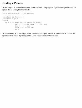
Creating a ProcessThe next step is to write Process code for the summer. Using expect to get a message and send forreplies, this is a straightforward task:

import Control.Distributed.Process

summerProc :: Process ()summerProc = go 0 where go s = do msg@(Add num from) <- expect say $ "received msg: " ++ show msg let s' = s + num send from (Value s') go s'

The say function is for debug purposes. By default, it outputs a string to standard error stream, butimplementation varies depending on the Cloud Haskell transport layer used.

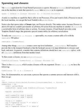
Spawning and closuresThe forkIO equivalent for Cloud Haskell processes is spawn. Because a Process doesn't necessarilyrun on the machine or node that spawns it, spawn takes a NodeId as its argument:

spawn :: NodeId -> Closure (Process ()) -> Process ProcessId

A node is a machine or capability that is able to run Processes. If we just want to fork a Process to run onthe local machine, we can get the local NodeId with getSelfNode.

Notice also that spawn takes a Closure type, not Process directly. This makes sense, because Process isakin to IO and we couldn't just transfer an arbitrary IO action from one machine to another. A Closure isa serializable form of arbitrary data or actions. To create closures, Cloud Haskell provides someTemplate Haskell magic that generates special remote tables for arbitrary serialization.

To make our summerProc :: Process () spawnable, we create a remote table of it with theremotable TH splice:

remotable ['summerProc]

Among other things, remotable creates a new top-level definition __remoteTable. We'll need toprovide this to the transport backend so that the backend can use it to map definitions to closures andback, and more. In general, a module that contains definitions should have one remotable splice, withall remotable definitions from that module listed.

To then create a closure, we use mkStaticClosure:

$(mkStaticClosure 'summerProc) :: Closure (Process ())

There is also mkClosure, which creates closures with one argument. Given f :: a → b, we have thefollowing:

$(mkClosure 'f) :: a → Closure b

Now, for demonstration, we can create a process that spawns a summer process and interacts with it.Here we go:

[…]import Control.Distributed.Process.ClosuresummerTest :: Process ()summerTest = do node<- getSelfNode summerPid<- spawn node $(mkStaticClosure 'summerProc)

mypid<- getSelfPid

send summerPid (Add 5 mypid) send summerPid (Add 7 mypid)

Value n <- expect say $ "updated value: " ++ show n Value n'<- expect say $ "updated value: " ++ show n'

We use getSelfNode and getSelfPid to get the NodeId and ProcessId for the current process. We usespawn to create a new process from a closure, which gives us the ProcessId of the newly made process.We send messages to that, which in turn replies to us.

The final thing that's missing is the backend that initializes nodes and manages processes.

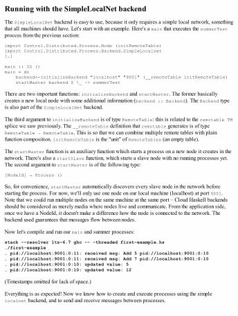
Running with the SimpleLocalNet backendThe SimpleLocalNet backend is easy to use, because it only requires a simple local network, somethingthat all machines should have. Let's start with an example. Here's a main that executes the summerTestprocess from the previous section:

import Control.Distributed.Process.Node (initRemoteTable)import Control.Distributed.Process.Backend.SimpleLocalnet[…]

main :: IO ()main = do backend<-initializeBackend "localhost" "9001" (__remoteTable initRemoteTable) startMaster backend $ \_ -> summerTest

There are two important functions: initializeBackend and startMaster. The former basicallycreates a new local node with some additional information (backend :: Backend). The Backend typeis also part of the SimpleLocalNet backend.

The third argument to initializeBackend is of type RemoteTable: this is related to the remotable THsplice we saw previously. The __remoteTable definition that remotable generates is of typeRemoteTable → RemoteTable. This is so that we can combine multiple remote tables with plainfunction composition. initRemoteTable is the "unit" of RemoteTables (an empty table).

The startMaster function is an auxiliary function which starts a process on a new node it creates in thenetwork. There's also a startSlave function, which starts a slave node with no running processes yet.The second argument to startMaster is of the following type:

[NodeId] → Process ()

So, for convenience, startMaster automatically discovers every slave node in the network beforestarting the process. For now, we'll only use one node on our local machine (localhost) at port 9001.Note that we could run multiple nodes on the same machine at the same port – Cloud Haskell backendsshould be considered as merely media where nodes live and communicate. From the application side,once we have a NodeId, it doesn't make a difference how the node is connected to the network. Thebackend used guarantees that messages flow between nodes.

Now let's compile and run our main and summer processes:

stack --resolver lts-6.7 ghc -- -threaded first-example.hs./first-example… pid://localhost:9001:0:11: received msg: Add 5 pid://localhost:9001:0:10… pid://localhost:9001:0:11: received msg: Add 7 pid://localhost:9001:0:10… pid://localhost:9001:0:10: updated value: 5… pid://localhost:9001:0:10: updated value: 12

(Timestamps omitted for lack of space.)

Everything is as expected! Now we know how to create and execute processes using the simplelocalnet backend, and to send and receive messages between processes.

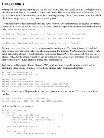
Using channelsWhile plain message-passing using expect and send works fine, it has some caveats. The biggest one isthat all messages from all processes go to the same queue. This has two unfortunate implications. First,expect has to search the queue every time for a matching message. Second, we cannot know from whichclient the message came, or if it is even relevant anymore.

Cloud Haskell provides an abstraction called typed channels to overcome these difficulties. A channelconsists of a SendPort and a ReceivePort that are connected to provide unidirectional communicationusing sendChan and receiveChan:

newChan :: (Typeable a, Binary a) => Process (SendPort a, ReceivePort a)

receiveChan :: (Typeable a, Binary a) => ReceivePort a -> Process a

sendChan :: (Typeable a, Binary a) => SendPort a -> a -> Process ()

Because SendPort is Serializable, we can send them using send. This way, it is easy to establishbidirectional communication between a client and server, for instance. What's more, the channel is onlyvalid through the lifetime of SendPort and corresponding ReceivePort. Messages can be put into thechannel only after the channel's creation, unlike with plain messaging, where messages flow as long asthe process is alive. Typed channels enable easy encapsulation.

Let's see a small example of using channels. We'll continue using a simple summer process just toemphasize Cloud Haskell features. First, a fairly minimal set of pragmas and imports:

-- file: client-server.hs{-# LANGUAGE BangPatterns #-}

import Control.Monadimport Control.Distributed.Processimport Control.Distributed.Process.Node (initRemoteTable)import Control.Distributed.Process.Backend.SimpleLocalnet

This time around, we will spawn clients that take a port to send numbers into. The client is a simpleone-liner:

client :: SendPort Double -> Process ()client sendport = forM_ [1..100] (sendChan sendport)

And here is the master process:

master :: Process ()master = do ports<- replicateM 100 $ do -- (1) (sendport, recvport) <- newChan _pid <- spawnLocal (client sendport) return recvport

port<- mergePortsRR ports -- (2)

let loop !s = do -- (3) mn<- receiveChanTimeout 1000 port

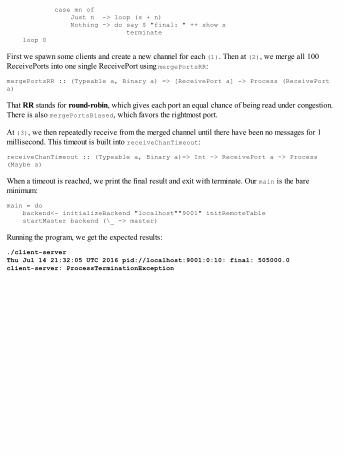
case mn of Just n -> loop (s + n) Nothing -> do say $ "final: " ++ show s terminate loop 0

First we spawn some clients and create a new channel for each (1). Then at (2), we merge all 100ReceivePorts into one single ReceivePort using mergePortsRR:

mergePortsRR :: (Typeable a, Binary a) => [ReceivePort a] -> Process (ReceivePort a)

That RR stands for round-robin, which gives each port an equal chance of being read under congestion.There is also mergePortsBiased, which favors the rightmost port.

At (3), we then repeatedly receive from the merged channel until there have been no messages for 1millisecond. This timeout is built into receiveChanTimeout:

receiveChanTimeout :: (Typeable a, Binary a)=> Int -> ReceivePort a -> Process (Maybe a)

When a timeout is reached, we print the final result and exit with terminate. Our main is the bareminimum:

main = do backend<- initializeBackend "localhost""9001" initRemoteTable startMaster backend (\_ -> master)

Running the program, we get the expected results:

./client-serverThu Jul 14 21:32:05 UTC 2016 pid://localhost:9001:0:10: final: 505000.0client-server: ProcessTerminationException

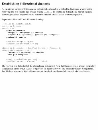
Establishing bidirectional channelsAs mentioned earlier, only the sending endpoint of a channel is serializable. So it must always be thereceiving end of a channel that creates it using newChan. To establish a bidirectional pair of channelsbetween processes, they both create a channel and send the sendport to the other process.

In practice, this would look like the following:

-- file: bi-directional.hsserver :: Process ()server = do pid<- getSelfPid (sendport', recvport) <- newChan _clientPid <- spawnLocal (client pid sendport') sendport<- expect

sendChan sendport "ping" receiveChan recvport >>= say

client :: ProcessId -> SendPort String -> Process ()client pid sendport = do (sendport', recvport) <- newChan send pid sendport'

ping<- receiveChan recvport sendChan sendport ("pong: " ++ ping)

The relevant bits that establish the channels are highlighted. Note that these processes are not completelysymmetrical, in that to run client we provide its master's process and upstream channel as arguments.But this isn't mandatory. With a bit more work, they both could establish channels via send/expect.

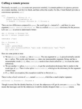
Calling a remote processPreviously, we used spawn to create new processes remotely. A common pattern is to spawn a processon a remote machine, wait for it to finish, and then collect the results. For this, Cloud Haskell provides aconvenience operation, call:

call :: (Typeable a, Binary a) => Static (SerializableDict a) -> NodeId -> Closure (Process a) -> Process a

There are two differences compared to spawn: the result type is a instead of () and there is a newargument, Static (SerializableDict a). This is a reified Serializable dictionary for the process.Let's see call in action to understand it better:

rpc :: String -> Process Intrpc str = return (length str)

remotable ['rpc]

foo :: Process ()foo = do node<- getSelfNode str<- call $(functionTDict 'rpc) node ($(mkClosure 'rpc) "foo") say (show str)

Here are some points to note:

We use mkClosure to turn rpc into a Closure. The one argument to rpc is passed normally outsidethe TH splice. This works only because rpc takes one monomorphic argument, String, and has amonomorphic result (Int). Also, remotable needs to have been called for rpc to create the staticdefinitions.We use another TH splice, functionTDict, to get the serialization dictionary that is similar to theresult type of rpc. There is also splice functionSDict, which gives the dictionary for the argument(source) type.If rpc threw an exception, this exception would be re-thrown at foo.

There is also a local version of call, named callLocal, which has a much simpler signature:

callLocal :: Process a → Process a

Though it seems like the identity function, it is not: the subprocess will get its own new ProcessId. Thismeans that messages sent for the subprocess would be silently dropped when callLocal returns.

Handling failureIn a distributed system, it's customary to fail fast and let other processes deal with failure. This principleis encouraged in Erlang, from which Cloud Haskell is modelled. We should be prepared for an arbitraryprocess crashing, with its parent or monitoring process handling the failure (or propagating it further to aparent's parent).

There are two tactics to be noted about process failure in Cloud Haskell: linking and monitoring. Thedifference is that a linked process propagates exceptions to its parent, while an exception in a monitoredprocess results in the monitoring process receiving a ProcessMonitorNotification message.

Firing up monitorsThe basic monitoring API is the following:

monitor :: ProcessId → Process MonitorRefmonitorNode :: NodeId → Process MonitorRefmonitorPort :: SendPort a → Process MonitorRef

unmonitor :: MonitorRef → Process ()

withMonitor :: ProcessId → Process a → Process a

We can start monitoring either a process, a node, or a channel. A MonitorRef is retained so that it'spossible to unmonitor later. The withMonitor combinator combines monitor and unmonitor, bymonitoring the process only when in the inner computation.

When a monitored process exits, a notification message is sent to the monitoring process. To catch themessage along with other messages in the system, we need some additional machinery. Plain expect isnot sufficient here, because it matches one type only.

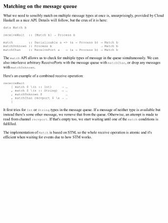
Matching on the message queueWhat we need to sensibly match on multiple message types at once is, unsurprisingly, provided by CloudHaskell as a nice API. Details will follow, but the crux of it is here:

data Match b

receiveWait :: [Match b] → Process b

match :: Serializable a => (a → Process b) → Match bmatchUnknown :: Process b → Match bmatchChan :: ReceivePort a → (a → Process b) → Match b

The match API allows us to check for multiple types of message in the queue simultaneously. We canalso interleave arbitrary ReceivePorts with the message queue with matchChan, or drop any messageswith matchUnknown.

Here's an example of a combined receive operation:

receiveWait [ match $ \(n :: Int) → … , match $ \(s :: String) → … , matchUnknown $ … , matchChan recvport $ \x → … ]

It first tries for Int or String types in the message queue. If a message of neither type is available butinstead there's some other message, we remove that from the queue. Otherwise, an attempt is made toread from channel recvport. If that's empty too, we start waiting until one of the match conditions isfulfilled.

The implementation of Match is based on STM, so the whole receive operation is atomic and it'sefficient when waiting for events due to how STM works.

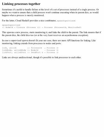
Linking processes togetherSometimes it's useful to handle failure at the level of a set of processes instead of a single process. Ormaybe we want to ensure that a child process won't continue executing when its parent dies, as wouldhappen when a process is merely monitored.

For the latter, Cloud Haskell provides a nice combinator, spawnSupervised:

spawnSupervised:: NodeId → Closure (Process ()) → Process (ProcessId, MonitorRef)

This spawns a new process, starts monitoring it, and links the child to the parent. The link ensures that ifthe parent dies, the child dies too (or at the very least receives an asynchronous exception).

In case a supervised spawn doesn't fit your use case, there are more API functions for linking. Likemonitoring, linking extends from processes to nodes and ports:

link, unlink :: ProcessId → Process ()linkNode, unlinkNode :: NodeId → Process ()linkPort, unlinkPort :: SendPort a → Process ()

Links are always unidirectional, though it's possible to link processes to each other.

Message-passing performanceIt's worth noting that message passing between processes normally goes between the network transportand undergoes serialization following deserialization. Serialization is not a free operation and it'sinevitable between processes located on different nodes. However, processes on the same node don'tnecessarily need to do the relatively expensive serialization at all.

Cloud Haskell takes a conservative approach and doesn't by default optimize local node communication.The main reason is that skipping (de)serialization can possibly give different runtime semantics due tostrictness. For instance, unnoticed bottoms can lurk in data that isn't fully forced. Messages sent overnetwork must always be fully evaluated, so it's easier for the developer when such mistakes can becaught in early development.

People familiar with distributed systems know that communication and serialization is not cheap, and inproduction it doesn't make much sense to incur extra work in local communication. Luckily, CloudHaskell does permit optimizing local communication. Unsafe send functions are provided in two places.The Control.Distributed.Process.UnsafePrimitives module replaces send functions from themain API, Control.Distributed.Process, while the main API provides unsafe variants with theunsafe prefix.

Using the unsafe variants is faster, but you will need to make sure you are not relying on evaluation-basedasynchronous exceptions getting thrown in any process: an unsafe send can result in the exception beingraised in the receiver instead of the sender.

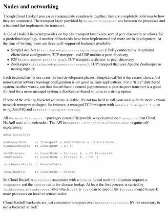
Nodes and networkingThough Cloud Haskell processes communicate seamlessly together, they are completely oblivious to howthey are connected. The transport layer provided by Network.Transport sits between the processes anda backend that implements the transport.

A Cloud Haskell backend provides on top of a transport layer some sort of peer discovery or allows fora predefined topology. A number of backends have been implemented and more are in development. Atthe time of writing, there are three well-supported backends available:

SimpleLocalNet (distributed-process-simplelocalnet): Fully connected with optionalclient/slave configuration, TCP transport, and UDP multicast peer discoveryP2P (distributed-process-p2p): TCP-transport with peer-to-peer discoveryZooKeeper (distributed-process-zookeeper): TCP transport that uses Apache ZooKeeper asnaming registry

Each backend has its use cases. In first development phases, SimpleLocalNet is the easiest choice, butnon-existent network topology configuration is not good in many applications. For a "truly" distributedsystem, in other words, one that doesn't have a central puppetmaster, a peer-to-peer transport is a goodfit. And for a more managed system, a ZooKeeper-based solution is a strong option.

If none of the existing backend solutions is viable, it's not too hard to roll your own with the more variousnetwork-transport packages, for instance, a managed TCP transport with network-transport-tcp orusing ZeroMQ and network-transport-zeromq.

All Network.Transport.* packages essentially provide ways to produce Transports that CloudHaskell uses to launch nodes. The API in Control.Distributed.Process.Node is quite self-explanatory:

data LocalNode

newLocalNode :: Transport → RemoteTable → IO LocalNodecloseLocalNode :: LocalNode → IO ()

forkProcess :: LocalNode → Process () → IO ProcessIdrunProcess :: LocalNode → Process () → IO ()

initRemoteTable :: RemoteTable

localNodeId :: LocalNode → NodeId

So Cloud Haskell's LocalNode associates with a NodeId. Local node initialization requires aTransport and the RemoteTable for closure lookup. At least the first process is started byforkProcess or runProcess, after which call or fork can be used in the Process monad to sparkmore processes on local or remote nodes.

Cloud Haskell backends are just convenient wrappers over network-transport. It's not necessary touse a backend in itself.

SummaryIn this chapter, we have learned to build distributed systems using the Cloud Haskell platform: launchingnodes and processes, communicating via direct message passing between processes and with moreflexible typed channels, passing remotely executed procedures in closures, and handling failure withprocess linking and monitoring. You now know how to build distributed systems with Cloud Haskell.

The next chapter will be about Functional Reactive Programming (FRP) and related Haskell libraries.Reactive programming, and especially FRP, challenges prevalent imperative control flow by a differentnotion of time. In imperative animation, for instance, timing is more or less implicit in the code, whereasin FRP, time would be just one more argument or input to an animation system. Reactive programmingextends beyond just animation, though.

Chapter 13. Functional Reactive ProgrammingFunctional Reactive Programming (FRP) is an elegant way to express behaviors that change over time,such as user interfaces or animation. From a theoretical point of view, behaviors are time-varying values.Using simple behaviors as building blocks, we can build increasingly complex behaviors: completeprograms, UIs, games, and so on. Behaviors compose very well and eliminate lots of tedious and error-prone work that's present in the traditional imperative approach with actions and callbacks.

Though FRP has simple semantics, efficient implementation is largely an open question. Existing FRPimplementations take different approaches with different trade-offs. In semantics, FRP is continuous, inother words, functions of the real numbers. In practice, we are forced to make approximations, either viasampling, using discrete semantics or some hybrid of continuous and discrete. The more theoreticallyminded reader is encouraged to glance at the following FRP papers: Functional Reactive Animation(1997, Elliot and Hudak), Push-Pull Functional Reactive Programming (2009, Elliot).

In this chapter, we will not bother much with understanding the semantics exactly. Instead, we will workwith simple but illustrative examples of FRP in practice using a few Haskell libraries that implementtheir own realizations of FRP: Elerea, Yampa, and Reactive-banana. Because there are so manyexamples, tutorials and additional libraries for hooking FRP logic into input and output sources, forexample, graphics frameworks, we won't focus on that aspect of FRP. Instead, the focus is on the verycore of FRP: elegant and powerful composition of behaviors and events.

This chapter will cover the following topics:

Programming with three FRP frameworks: Elerea, Yampa, and Reactive-bananaPros and cons of discrete- and continuous-time signals, events and behaviorsCoding recursion and mutual recursion in event networksAdding inputs and outputs to networks statically and dynamically

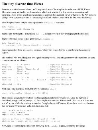
The tiny discrete-time ElereaIn order to not feel overwhelmed, we'll begin with one of the simplest formulations of FRP, Elerea.Elerea is a very minimalist implementation, which restricts itself to discrete-time semantics andsampling. There are no events and everything is computed on demand only. Furthermore, the API consistsof high-level constructs so that it's exceedingly difficult to shoot yourself in the foot with this library.

Time-varying values of type a are represented as Signal a in Elerea:

data Signal a-- instances incl. Monad, Eq

Signals can be thought of as functions Nat → a, though obviously they are represented differently.

Signals are made inside signal generators, SignalGen a:

data SignalGen a-- instances incl. Monad, MonadFix, MonadIO

Signal generators have a MonadFix instance, which will later allow us to build mutually recursivesignals.

The minimal API provides just a few signal building blocks. Excluding some trivial extensions, the corecombinators are as follows:

delay :: a → Signal a → SignalGen (Signal a)snapshot :: Signal a → SignalGen agenerator :: Signal (SignalGen a) → SignalGen (Signal a)memo :: Signal a → SignalGen (Signal a)till :: Signal Bool → SignalGen (Signal Bool)

stateful :: a → (a → a) → SignalGen (Sinal a)transfer :: a → (t → a → a) → Signal t → SignalGen (Signal a)

effectful :: IO a → SignalGen (Signal a)

We'll see some examples soon, but first we introduce start:

start :: SignalGen (Signal a) → IO (IO a)

This embeds a signal network built via the signal generator network into IO. Once the network isinitialized, we get an IO action (IO a) that samples the network. We can think of start as a "start-the-world" action while the resulting action is a "sample-the-world" action. We define a sigtest functionthat performs 10 samplings and prints them as a list:

-- file: elerea-first-ex.hsimport Control.Monadimport FRP.Elerea.Simple

sigtest :: Show a => SignalGen (Signal a) -> IO ()sigtest gen = start gen >>= replicateM 10 >>= print

Now, let's see some signals in action. First, we have stateful signals, similar to unfolding:

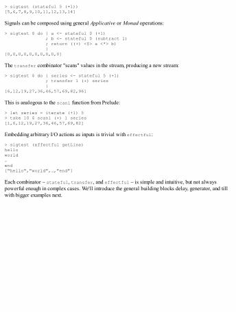
> sigtest (stateful 5 (+1))[5,6,7,8,9,10,11,12,13,14]

Signals can be composed using general Applicative or Monad operations:

> sigtest $ do { a <- stateful 0 (+1) ; b <- stateful 0 (subtract 1) ; return ((+) <$> a <*> b) }[0,0,0,0,0,0,0,0,0,0]

The transfer combinator "scans" values in the stream, producing a new stream:

> sigtest $ do { series <- stateful 5 (+1) ; transfer 1 (+) series }[6,12,19,27,36,46,57,69,82,96]

This is analogous to the scanl function from Prelude:

> let series = iterate (+1) 5> take 10 $ scanl (+) 1 series[1,6,12,19,27,36,46,57,69,82]

Embedding arbitrary I/O actions as inputs is trivial with effectful:

> sigtest (effectful getLine)helloworld…end["hello","world",…,"end"]

Each combinator – stateful, transfer, and effectful – is simple and intuitive, but not alwayspowerful enough in complex cases. We'll introduce the general building blocks delay, generator, and tillwith bigger examples next.

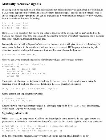
Mutually recursive signalsIn a complex FRP application, we often need signals that depend mutually on each other. For instance, ina UI, actions depend on user input and available input depends on past actions. The Fibonacci series isone of simplest example programs that can be expressed as a combination of mutually recursive signals.In pseudo-code we have the following:

fib <- 1 `cons` fib1fib1 <- 1 `cons` fib2let fib2 = fib + fib1

Here, cons is an operation that inserts one value to the head of the stream. But we can't quite directlytranslate this pseudo-code to SignalGen code, because the bindings are mutually recursive and a monadicbind is not recursive, though let bindings are.

Fortunately, we can utilize SignalGen's MonadFix instance, which will give us recursive bindings. Inorder to not bother with the details, we will use the RecursiveDo GHC language extension to yieldrecursive monadic bindings that look almost identical to normal monadic bindings:

{-# LANGUAGE RecursiveDo #-}

Now we can write a mutually recursive signal that produces the Fibonacci numbers:

fibonacci :: SignalGen (Signal Int)fibonacci = do rec fib <- delay 1 fib1 fib1 <- delay 1 fib2 let fib2 = (+) <$> fib <*> fib1 return fib

The magic is in the new rec keyword introduced by RecursiveDo. It lets us introduce a mutuallyrecursive group of bindings. The delay function is the cons operation on signals:

delay :: a -> Signal a -> SignalGen (Signal a)

Just to confirm our implementation works:

> sigtest fibonacci [1,1,2,3,5,8,13,21,34,55]

RecursiveDo is really just syntactic sugar: all the magic happens in the MonadFix class and instance,which doesn't depend on any magic at all.

Signalling side-effects

With effectful, it's easy to turn IO effects into input signals in the network. To use signal output as aparameter to a side effect, we can use variants of effectful that take the signal to bind to as parameter:

effectful1 :: (t -> IO a) -> Signal t -> SignalGen (Signal a)effectful2 :: (t1 -> t2 -> IO a)-> Signal t1 -> Signal t2 -> SignalGen (Signal a)

In the following small program, on every line read outputs the sum of read numbers so far:

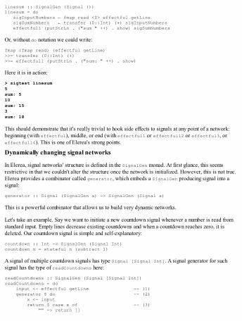
linesum :: SignalGen (Signal ())linesum = do sigInputNumbers ← fmap read <$> effectful getLine sigSumNumbers ← transfer (0::Int) (+) sigInputNumbers effectful1 (putStrLn . ("sum " ++) . show) sigSumNumbers

Or, without do notation we could write:

fmap (fmap read) (effectful getLine)>>= transfer (0::Int) (+)>>= effectful1 (putStrLn . ("sum: " ++) . show)

Here it is in action:

> sigtest linesum5sum: 510sum: 153sum: 18

This should demonstrate that it's really trivial to hook side effects to signals at any point of a network:beginning (with effectful), middle, or end (with effectful1 or effectfull2 or effectful3, oreffectfull4). This is one of Elerea's strong points.

Dynamically changing signal networks

In Elerea, signal networks' structure is defined in the SignalGen monad. At first glance, this seemsrestrictive in that we couldn't alter the structure once the network is initialized. However, this is not true.Elerea provides a combinator called generator, which embeds a SignalGen producing signal into asignal:

generator :: Signal (SignalGen a) -> SignalGen (Signal a)

This is a powerful combinator that allows us to build very dynamic networks.

Let's take an example. Say we want to initiate a new countdown signal whenever a number is read fromstandard input. Empty lines decrease existing countdowns and when a countdown reaches zero, it isdeleted. Our countdown signal is simple and self-explanatory:

countdown :: Int -> SignalGen (Signal Int)countdown n = stateful n (subtract 1)

A signal of multiple countdown signals has type Signal [Signal Int]. A signal generator for suchsignal has the type of readCountdowns here:

readCountdowns :: SignalGen (Signal [Signal Int])readCountdowns = do input <- effectful getLine -- (1) generator $ do -- (2) x <- input return $ case x of -- (3) "" -> return []

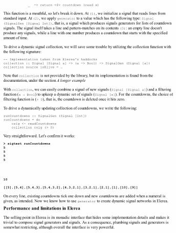
_ -> return <$> countdown (read x)

This function is a mouthful, so let's break it down. At (1), we initialize a signal that reads lines fromstandard input. At (2), we apply generator to a value which has the following type: Signal(SignalGen [Signal Int]), that is, a signal which produces signals generators for lists of countdownsignals. The signal itself takes a line and pattern-matches on its contents (3): an empty line doesn'tproduce any signals, while a line with one number produces a countdown that starts with the specifiedamount of time.

To drive a dynamic signal collection, we will save some trouble by utilizing the collection function withthe following signature:

-- Implementation taken from Elerea's haddockscollection :: Signal [Signal a] -> (a -> Bool) -> SignalGen (Signal [a])collection source isAlive = …

Note that collection is not provided by the library, but its implementation is found from thedocumentation, under the section A longer example

With collection, we can easily combine a signal of new signals (Signal [Signal a]) and a filteringfunction (a → Bool) to upkeep a dynamic set of signals (Signal [a]). For the countdowns, the choice offiltering function is (> 0), that is, the countdown is deleted once it hits zero.

To drive a dynamically updating collection of countdowns, we write the following:

runCountdowns :: SignalGen (Signal [Int])runCountdowns = do csig <- readCountdowns collection csig (> 0)

Very straightforward. Let's confirm it works:

> sigtest runCountdowns5555

10

[[5],[5,4],[5,4,3],[5,4,3,2],[4,3,2,1],[3,2,1],[2,1],[1],[10],[9]]

On every line, existing countdowns tick one down and new countdowns are added when a numeral isgiven, as intended. Now we know how to use generator to create dynamic signal networks in Elerea.

Performance and limitations in Elerea

The selling point in Elerea is its monadic interface that hides some implementation details and makes ittrivial to compose signal generators and signals. As a consequence, plumbing signals and generators issomewhat restricting, although overall the interface is very powerful.

The biggest concern with Elerea is its eventless nature: every time, the signal network updates as awhole. It's not possible to update just a part of the network; on every tick, all signals are re-calculated.By using the memo primitive, we can memoize values within one update round, but this is always manualwork. The library combinators memoize their values, but memoizing custom combinations is left to thelibrary user.

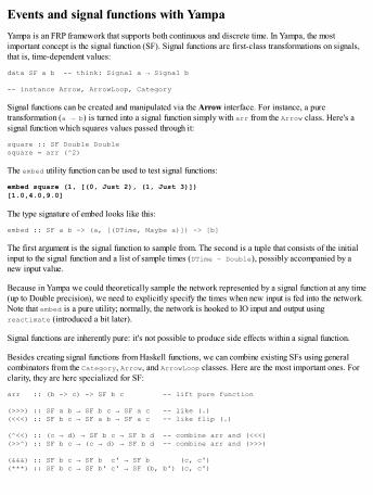
Events and signal functions with YampaYampa is an FRP framework that supports both continuous and discrete time. In Yampa, the mostimportant concept is the signal function (SF). Signal functions are first-class transformations on signals,that is, time-dependent values:

data SF a b -- think: Signal a → Signal b

-- instance Arrow, ArrowLoop, Category

Signal functions can be created and manipulated via the Arrow interface. For instance, a puretransformation (a → b) is turned into a signal function simply with arr from the Arrow class. Here's asignal function which squares values passed through it:

square :: SF Double Doublesquare = arr (^2)

The embed utility function can be used to test signal functions:

embed square (1, [(0, Just 2), (1, Just 3)])[1.0,4.0,9.0]

The type signature of embed looks like this:

embed :: SF a b -> (a, [(DTime, Maybe a)]) -> [b]

The first argument is the signal function to sample from. The second is a tuple that consists of the initialinput to the signal function and a list of sample times (DTime ~ Double), possibly accompanied by anew input value.

Because in Yampa we could theoretically sample the network represented by a signal function at any time(up to Double precision), we need to explicitly specify the times when new input is fed into the network.Note that embed is a pure utility; normally, the network is hooked to IO input and output usingreactimate (introduced a bit later).

Signal functions are inherently pure: it's not possible to produce side effects within a signal function.

Besides creating signal functions from Haskell functions, we can combine existing SFs using generalcombinators from the Category, Arrow, and ArrowLoop classes. Here are the most important ones. Forclarity, they are here specialized for SF:

arr :: (b -> c) -> SF b c -- lift pure function

(>>>) :: SF a b → SF b c → SF a c -- like (.)(<<<) :: SF b c → SF a b → SF a c -- like flip (.)

(^<<) :: (c → d) → SF b c → SF b d -- combine arr and (<<<)(>>^) :: SF b c → (c → d) → SF b d -- combine arr and (>>>)

(&&&) :: SF b c → SF b c' → SF b (c, c')(***) :: SF b c → SF b' c' → SF (b, b') (c, c')

loop :: SF (b, d) (c, d) -> SF b c -- SF with feed-back

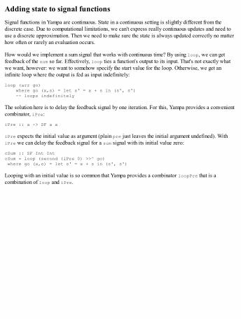
Adding state to signal functionsSignal functions in Yampa are continuous. State in a continuous setting is slightly different from thediscrete case. Due to computational limitations, we can't express really continuous updates and need touse a discrete approximation. Then we need to make sure the state is always updated correctly no matterhow often or rarely an evaluation occurs.

How would we implement a sum signal that works with continuous time? By using loop, we can getfeedback of the sum so far. Effectively, loop ties a function's output to its input. That's not exactly whatwe want, however: we want to somehow specify the start value for the loop. Otherwise, we get aninfinite loop where the output is fed as input indefinitely:

loop (arr go) where go (x,s) = let s' = x + s in (s', s') -- loops indefinitely

The solution here is to delay the feedback signal by one iteration. For this, Yampa provides a convenientcombinator, iPre:

iPre :: a -> SF a a

iPre expects the initial value as argument (plain pre just leaves the initial argument undefined). WithiPre we can delay the feedback signal for a sum signal with its initial value zero:

cSum :: SF Int IntcSum = loop (second (iPre 0) >>^ go) where go (x,s) = let s' = x + s in (s', s')

Looping with an initial value is so common that Yampa provides a combinator loopPre that is acombination of loop and iPre.

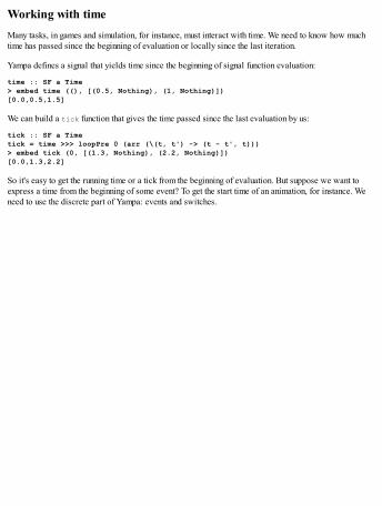
Working with timeMany tasks, in games and simulation, for instance, must interact with time. We need to know how muchtime has passed since the beginning of evaluation or locally since the last iteration.

Yampa defines a signal that yields time since the beginning of signal function evaluation:

time :: SF a Time> embed time ((), [(0.5, Nothing), (1, Nothing)])[0.0,0.5,1.5]

We can build a tick function that gives the time passed since the last evaluation by us:

tick :: SF a Timetick = time >>> loopPre 0 (arr (\(t, t') -> (t - t', t)))> embed tick (0, [(1.3, Nothing), (2.2, Nothing)])[0.0,1.3,2.2]

So it's easy to get the running time or a tick from the beginning of evaluation. But suppose we want toexpress a time from the beginning of some event? To get the start time of an animation, for instance. Weneed to use the discrete part of Yampa: events and switches.

Switching and discrete-time eventsYampa supports discrete-time FRP via events and switches. An event containing a value of type a isrepresented by Event a:

data Event a = Event a | NoEvent-- instance Monad, Alternative, …

An event source is a signal function with some type SF a (Event b). Some example event sources areas follows:

never :: SF a (Event b)now :: b → SF a (Event b)after :: Time → b → SF a (Event b)

Because event source is just a normal SF, we could yield events with arr. However, then we should takecare that the event is emitted only once: because signal functions are continuous, unless the event issuppressed on subsequent samplings, it could occur more than once.

To react on events, we need switches. The basic one-time switch has the following type:

switch :: SF a (b, Event c) -- Default signal -> (c → SF a b) -- Signal after event -> SF a b

The following signal yields the string foo for first 2 seconds, after which an event is fired and bar isyielded:

switchFooBar, switchFooBar' :: SF () String

switchFooBar = switch (constant "foo"&&& after 2 "bar") constantswitchFooBar' = dSwitch (constant "foo"&&& after 2 "bar") constant

Function dSwitch is identical to switch except that, at the time of the event, the previous signal isyielded one more time. The following shows the difference:

> embed switchFooBar ((), [(2, Nothing), (3, Nothing)])["foo","bar","bar"]> embed switchFooBar' ((), [(2, Nothing), (3, Nothing)])["foo","foo","bar"]

This is a one-time switch: once the event occurs, we switch permanently to the new signal function. Toswitch on more events, we can apply switch recursively. For instance, this signal alternates betweenfoo and bar every 2 seconds:

switchRec :: SF () StringswitchRec = go (0, "foo", "bar") where go (t, x, y) = switch (constant x &&& after (t + 2) (t + 2, y, x)) go

Here, time for the after combinator is just threaded through as an argument. Note that the time signal andTime arguments are always relative to current evaluation context, irrespective of switching.

Another switch combinator is rSwitch (and its delayed version, drSwitch). This recurring switchaccepts whole signal functions as events, and every time replaces the active SF with newly emitted SF.Take a look at its type:

rSwitch :: SF a b -> SF (a, Event (SF a b)) b

The first argument is the initial SF a b. Resulting SF expects an Event (SF a b) stream tupled withactual input a.

An example use of a recurring switch would be changing walk directions in a game, say between foo andbar. We can write this as follows:

swap :: SF Bool Stringswap = rSwitch foo <<< identity &&& swapEv -- (1) where swapEv = edge >>> sscanPrim go True (Event foo) -- (2)

go tag = event Nothing $ \_ -> -- (3) Just (not tag, Event $ if tag then bar else foo)

foo = constant "foo" bar = constant "bar"

Here, swap is an SF that reads, for instance, a button press status as a Boolean. Its output alternatesbetween foo and bar, so that every button press (from pressed to unpressed; False to True) triggers aswitch. At (1), the Boolean input signal is tupled into the original signal and an event signal (swapEv),which is fed into rSwitch.

The event signal at (2) applies an edge detector transformation (edge) from the Yampa API. It yields anevent every time an edge is detected in the input signal:

edge :: SF Bool (Event ())

In the second step, we scan over the Event signal with sscanPrim and on every triggered event yield anSF different from the previously active (foo or bar). The tag in (3) indicates which of the SFs iscurrently active. The combinators here are:

sscanPrim :: (c -> a -> Maybe (c, b)) -> c -> b -> SF a b

event :: a -> (b -> a) -> Event b -> a

Confirm our swap works as intended:

> embed swap (True, zip [1..] (map Just [False, False, True, False, True]))["foo","foo","foo","bar","bar","foo"]

The third type of switch is perhaps the hardest to understand. It's called a call-with-current-continuationswitch, kSwitch, or its delayed version, dkSwitch. Its type is:

kSwitch :: SF a b - initial SF -> SF (a, b) (Event c) - event trigger -> (SF a b -> c -> SF a b) – continuation SF -> SF a b

This switch allows access to the previous SF when deciding the continuation based on an event. We canchoose to use the current SF in the new SF, for instance, as a pre- or post-processor. Like a normalswitch, kSwitch switches only once. The difference is that deciding the continuation (third argument) iscompletely decoupled from the initial SF and event trigger. kSwitch composes a bit better thanswitch.

As a rather artificial example, we have the following SF:

withCC :: SF Int IntwithCC = kSwitch (arr (+1)) trigger cont where trigger = sscan f NoEvent

f _ (inp,_) | inp > 1 && inp < 10 = Event (*inp) | otherwise = NoEvent

cont f f' = f >>> arr f'

Initially, this SF adds 1 to every number in the stream. When a number larger than 1 and smaller than 10is encountered, from that point onward the numbers are also multiplied by that number. Note how indeciding the continuation (cont), we don't know or care about the specifics of the initial SF, but we canuse it as a part of the final SF.

Example run:

> embed withCC (1, zip [1..10] (map Just [10,2,10,3,10]))[2,11,6,22,8,22]

Integrating to the real worldIn all Yampa examples so far, we have simulated the pure signal functions with embed. Signal functionsare pure, so pure simulation is always possible. However, in real applications, we want to integrate SFinto a loop with the real world, IO. Because signal functions store state, mere multiple calls to embedwould be insufficient. We need to preserve the state somehow.

For the simplest cases, Yampa provides a single combinator that guides us through the integration. It'scalled reactimate and its type is:

reactimate :: IO a -- Init -> (Bool -> IO (DTime, Maybe a)) -- Get input -> (Bool -> b -> IO Bool) -- Process output -> SF a b -- Signal function -> IO ()

Besides the SF to execute, we need to define three IO actions: one to supply the initial input to the SF,one to sense input, and one to actuate output.

The sense function is informed via an argument whether it can block or not. The sense result should be atuple of time difference since the last iteration and new input (if any).

The actuation is informed via an argument whether the output has changed since the last actuation. Whenthe actuation returns True, reactimation stops there.

However, in practice, reactimate always calls the sense function with False (no block) and theactuation function with True (has changed). These arguments have no effect in Yampa version 0.10.5 atleast.

The following main reads numbers from standard input and adds them together until hitting 42 or more,after which it exits:

main = reactimate init sense actuate sf where init = return "0"

sense _ = do ln <- getLine return (1, Just ln)

actuate _ out = do putStrLn out return (out == "END")

sf = arr read >>> sscan (+) 0 >>> dSwitch (arr show &&& arr (filterE (>= 42) . Event)) (\_ -> constant "END")

In complex applications, it isn't feasible to make reactimate the main loop of the program. Thealternative is to use reactInit to yield a ReactHandle and react to feed input to it. Essentially these

two functions decompose reactimate to two parts that allow for more flexibility.

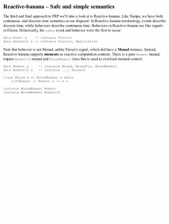
Reactive-banana – Safe and simple semanticsThe third and final approach to FRP we'll take a look at is Reactive-banana. Like Yampa, we have bothcontinuous- and discrete-time semantics at our disposal. In Reactive-banana terminology, events describediscrete time, while behaviors describe continuous time. Behaviors in Reactive-banana are like signalsin Elerea. Historically, the names event and behavior were the first to occur:

data Event a -- instance Functordata Behavior a -- instance Functor, Applicative

Note that behavior is not Monad, unlike Elerea's signal, which did have a Monad instance. Instead,Reactive-banana supports moments as reactive computation contexts. There is a pure Moment monad,impure MomentIO monad and MonadMoment class that is used to overload moment context:

data Moment a -- instance Monad, MonadFix, MonadMomentdata MomentIO a –- instance ..., MonadIO

class Monad m => MonadMoment m where liftMoment :: Moment a -> m a

instance MonadMoment Momentinstance MonadMoment MomentIO

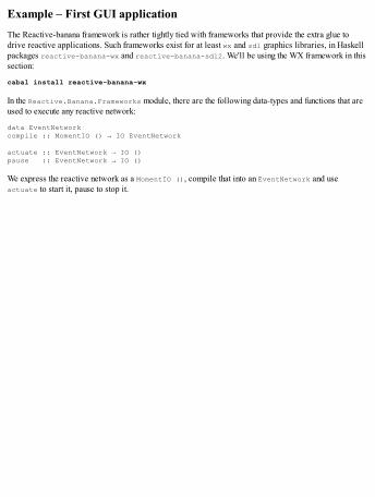
Example – First GUI applicationThe Reactive-banana framework is rather tightly tied with frameworks that provide the extra glue todrive reactive applications. Such frameworks exist for at least wx and sdl graphics libraries, in Haskellpackages reactive-banana-wx and reactive-banana-sdl2. We'll be using the WX framework in thissection:

cabal install reactive-banana-wx

In the Reactive.Banana.Frameworks module, there are the following data-types and functions that areused to execute any reactive network:

data EventNetworkcompile :: MomentIO () → IO EventNetwork

actuate :: EventNetwork → IO ()pause :: EventNetwork → IO ()

We express the reactive network as a MomentIO (), compile that into an EventNetwork and useactuate to start it, pause to stop it.

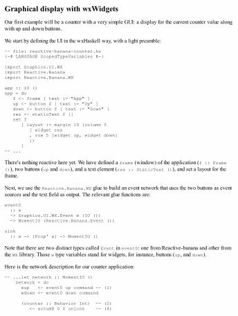
Graphical display with wxWidgetsOur first example will be a counter with a very simple GUI: a display for the current counter value alongwith up and down buttons.

We start by defining the UI in the wxHaskell way, with a light preamble:

-- file: reactive-banana-counter.hs{-# LANGUAGE ScopedTypeVariables #-}

import Graphics.UI.WXimport Reactive.Bananaimport Reactive.Banana.WX

app :: IO ()app = do f <- frame [ text := "App" ] up <- button f [ text := "Up" ] down <- button f [ text := "Down" ] res <- staticText f [] set f [ layout := margin 10 (column 5 [ widget res , row 5 [widget up, widget down] ]) ]-- ...

There's nothing reactive here yet. We have defined a frame (window) of the application (f :: Frame()), two buttons (up and down), and a text element (res :: StaticText ()), and set a layout for theframe.

Next, we use the Reactive.Banana.WX glue to build an event network that uses the two buttons as eventsources and the text field as output. The relevant glue functions are:

event0 :: w -> Graphics.UI.WX.Event w (IO ()) -> MomentIO (Reactive.Banana.Event ())

sink :: w -> [Prop' w] -> MomentIO ()

Note that there are two distinct types called Event in event0: one from Reactive-banana and other fromthe WX library. Those w type variables stand for widgets, for instance, buttons (up, and down).

Here is the network description for our counter application:

-- ...let network :: MomentIO () network = do eup <- event0 up command -- (1) edown <- event0 down command

(counter :: Behavior Int) -- (2) <- accumB 0 $ unions –- (4)

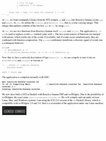
[ (+1) <$ eup , subtract 1 <$ edown ]

sink res [ text :== show <$> counter ] -- (3)-- ...

At (1), we bind commands (clicks) from the WX widgets up and down into Reactive-banana events eupand edown. At (2), we define the counter as a Behavior Int, that is, a time-varying integer. Thatinteger then updates contents of the text box res at (3) by using sink.

At (4), we use two functions from Reactive-banana itself: accumB and unions. The applicative (a <$ev) is used to replace event's ev emitted value with a. The two event sources of functions are mergedwith unions, which yields any of the events if available, and if events occur simultaneously, they arecombined with function composition. The accumB combinator transforms a discrete signal of events intoa continuous behavior:

accumB :: MonadMoment m => a -> Reactive.Banana.Event (a -> a) -> m (Behavior a)

Now that we have a network description of type MomentIO (), we use compile to turn it into anEventNetwork and actuate to execute it:

-- ...evnet <- compile network actuate evnet

main = start app

The application is compiled normally with GHC:

ghc reactive-banana-counter.hs[1 of 1] Compiling Main ( reactive-banana-counter.hs, reactive-banana-counter.o )Linking reactive-banana-counter …

We now have built a GUI in Haskell with Reactive-banana FRP and wxWidgets. Due to the portability ofwxWidgets, the exact same reactive-banana-counter.hs file will compile and run under at leastLinux, Mac, and Windows systems. I am using the 0.92.2.0 version of the wx Haskell library, which iscompatible with wxWidgets 2.9 and 3.0. Here's a screenshot of the application under one Linux machine:

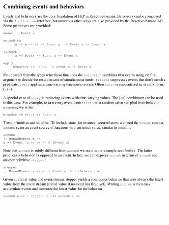
Combining events and behaviorsEvents and behaviors are the core foundation of FRP in Reactive-banana. Behaviors can be composedvia the Applicative interface, but numerous other ways are also provided by the Reactive-banana API.Some primitives are provided:

never :: Event a

unionWith :: (a -> a -> a) -> Event a -> Event a -> Event a

filterE :: (a -> Bool) -> Event a -> Event a

apply :: Behavior (a -> b) -> Event a -> Event b

It's apparent from the types what these functions do. unionWith combines two events using the firstargument to decide the result in case of simultaneous emits. filterE suppresses events that don't match apredicate. apply applies a time-varying function to events. Often apply is encountered in its infix form,(<@>).

A special case of apply is replacing events with time-varying values. The (<@) combinator can be usedin this case. For example, to turn every event from etick into a random value sampled from behaviorbrandom, we write:

brandom <@ etick :: Event a

These primitives are stateless. To include state, for instance, accumulators, we need the Moment context.accumE scans an event source of functions with an initial value, similar to scanl':

accumE:: MonadMoment m =>a -> Event (a -> a) -> m (Event a)

Note that accumE is subtly different from accumB we used in our example seen before. The latterproduces a behavior as opposed to an event. In fact, we can express accumB in terms of accumE andanother primitive stepper:

stepper:: MonadMoment m => a -> Event a -> m (Behavior a)

Given an initial value and event stream, stepper yields a continuous behavior that uses always the latestvalue from the event stream (initial value if no event has fired yet). Writing accumB is then easy:accumulate events and memoize the latest value for the behavior:

accumB a ev = stepper a =<< accumE a ev

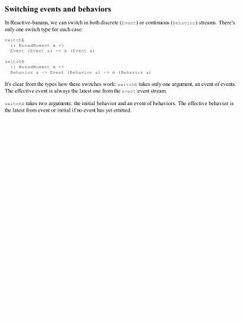
Switching events and behaviorsIn Reactive-banana, we can switch in both discrete (Event) or continuous (Behavior) streams. There'sonly one switch type for each case:

switchE :: MonadMoment m => Event (Event a) -> m (Event a)

switchB :: MonadMoment m => Behavior a -> Event (Behavior a) -> m (Behavior a)

It's clear from the types how these switches work: switchE takes only one argument, an event of events.The effective event is always the latest one from the event event stream.

switchB takes two arguments: the initial behavior and an event of behaviors. The effective behavior isthe latest from event or initial if no event has yet emitted.

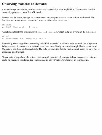
Observing moments on demandAlmost always, there is only one MonadMoment computation in an application. That moment is whateventually gets turned to an EventNetwork.

In some special cases, it might be convenient to execute pure Moment computations on demand. Thefunction that executes moments emitted in an event is called observeE:

observeE:: Event (Moment a) -> Event a

A useful combinator to use along with observeE is valueB, which samples a value of the Behavior:

valueB:: MonadMoment m => Behavior a -> m a

Essentially, observing allows executing "mini FRP networks" within the main network in a single step.When a Moment in a network is emitted, observeE immediately executes it and yields the result value.The network is discarded immediately. The only constraint is that the mini network has to be pure, that is,expressed as a Moment.

Nested networks probably have their uses. A small uncontrived example is hard to conceive, but onecould be running a simulation that is expressed as an FRP network whenever an event occurs.

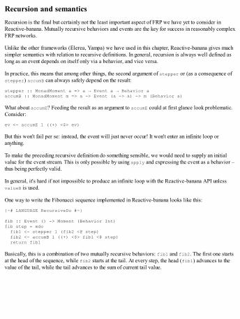
Recursion and semanticsRecursion is the final but certainly not the least important aspect of FRP we have yet to consider inReactive-banana. Mutually recursive behaviors and events are the key for success in reasonably complexFRP networks.

Unlike the other frameworks (Elerea, Yampa) we have used in this chapter, Reactive-banana gives muchsimpler semantics with relation to recursive definitions. In general, recursion is always well defined aslong as an event depends on itself only via a behavior, and vice versa.

In practice, this means that among other things, the second argument of stepper or (as a consequence ofstepper) accumB can always safely depend on the result:

stepper :: MonadMoment a => a → Event a → Behavior aaccumB :: MonadMoment m => a -> Event (a -> a) -> m (Behavior a)

What about accumE? Feeding the result as an argument to accumE could at first glance look problematic.Consider:

ev <- accumE 1 ((+) <$> ev)

But this won't fail per se: instead, the event will just never occur! It won't enter an infinite loop oranything.

To make the preceding recursive definition do something sensible, we would need to supply an initialvalue for the event stream. This is only possible by using apply and expressing the event as a behavior –thus being perfectly valid.

In general, it's hard if not impossible to produce an infinite loop with the Reactive-banana API unlessvalueB is used.

One way to write the Fibonacci sequence implemented in Reactive-banana looks like this:

{-# LANGUAGE RecursiveDo #-}

fib :: Event () -> Moment (Behavior Int)fib step = mdo fib1 <- stepper 1 (fib2 <@ step) fib2 <- accumB 1 ((+) <$> fib1 <@ step) return fib1

Basically, this is a combination of two mutually recursive behaviors: fib1 and fib2. The first one startsat the head of the sequence, while fib2 starts at the tail. At every step, the head (fib1) advances to thevalue of the tail, while the tail advances to the sum of current tail value.

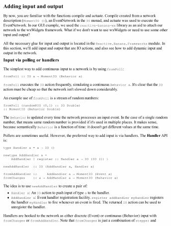
Adding input and outputBy now, you are familiar with the functions compile and actuate. Compile created from a networkdescription (MomentIO ()), an EventNetwork in the IO monad, and actuate was used to execute theEventNetwork. In our GUI example, we used the reactive-banana-wx library as an aid to attach ournetwork to the wxWidgets framework. What if we don't want to use wxWidgets or need to use some otherinput and output?

All the necessary glue for input and output is located in the Reactive.Banana.Frameworks module. Inthis section, we'll add input and output that are IO actions, and also see how to add dynamic input andoutput in the network.

Input via polling or handlers

The simplest way to add continuous input to a network is by using fromPoll:

fromPoll :: IO a → MomentIO (Behavior a)

fromPoll executes the IO action frequently, simulating a continuous Behavior a. It's clear that the IOaction must be cheap so that the network isn't slowed down considerably.

An example use of fromPoll is a stream of random numbers:

fromPoll (randomRIO (0,1) :: IO Double):: MomentIO (Behavior Double)

The Behavior is updated every time the network processes an input event. In the case of a single randomnumber, that means same random number is provided if it's used in multiple places. It makes sense,because semantically Behavior is a function of time: it doesn't get different values at the same time.

Pollers are sometimes useful. However, the preferred way to add input is via handlers. The Handler APIis:

type Handler a = a → IO ()

newtype AddHandler a = AddHandler { register :: Handler a → IO (IO ()) }

newAddHandler :: IO (AddHandler a, Handler a)

fromAddHandler :: AddHandler a → MomentIO (Event a)fromChanges :: a → AddHandler a → MomentIO (Behavior a)

The idea is to use newAddHandler to create a pair of:

Handler a: An IO action to push input of type a to the handler.AddHandler a: Event handler registration facility. register addHandler myHandler registersthe handler myHandler to fire whenever an event is fired. The returned IO action can be used tounregister the handler.

Handlers are hooked to the network as either discrete (Event) or continuous (Behavior) input withfromChanges or fromAddHandler. Note that fromChanges is just a combination of stepper and

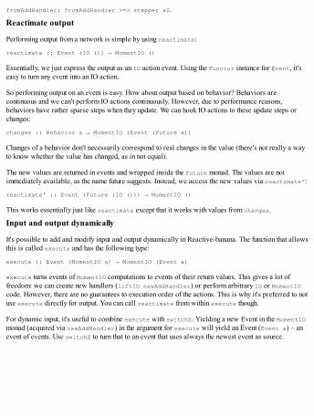
fromAddHandler: fromAddHandler >=> stepper x0.

Reactimate output

Performing output from a network is simple by using reactimate:

reactimate :: Event (IO ()) → MomentIO ()

Essentially, we just express the output as an IO action event. Using the Functor instance for Event, it'seasy to turn any event into an IO action.

So performing output on an event is easy. How about output based on behavior? Behaviors arecontinuous and we can't perform IO actions continuously. However, due to performance reasons,behaviors have rather sparse steps when they update. We can hook IO actions to these update steps orchanges:

changes :: Behavior a → MomentIO (Event (Future a))

Changes of a behavior don't necessarily correspond to real changes in the value (there's not really a wayto know whether the value has changed, as in not equal).

The new values are returned in events and wrapped inside the Future monad. The values are notimmediately available, as the name future suggests. Instead, we access the new values via reactimate':

reactimate' :: Event (Future (IO ())) → MomentIO ()

This works essentially just like reactimate except that it works with values from changes.

Input and output dynamically

It's possible to add and modify input and output dynamically in Reactive-banana. The function that allowsthis is called execute and has the following type:

execute :: Event (MomentIO a) → MomentIO (Event a)

execute turns events of MomentIO computations to events of their return values. This gives a lot offreedom: we can create new handlers (liftIO newAddHandler) or perform arbitrary IO or MomentIOcode. However, there are no guarantees to execution order of the actions. This is why it's preferred to notuse execute directly for output. You can call reactimate from within execute though.

For dynamic input, it's useful to combine execute with switchE. Yielding a new Event in the MomentIOmonad (acquired via newAddHandler) in the argument for execute will yield an Event (Event a) – anevent of events. Use switchE to turn that to an event that uses always the newest event as source.

SummaryIn this chapter, we have worked with three different approaches to FRP: Elerea, with its safe monadicinterface and discrete-only signals; Yampa and its first-class signal functions; and finally, Reactive-banana and its safe and simple hybrid semantics. Implementation differences are rather radical, but thetheoretical FRP basis is still the same: model values as functions of time and include discrete events. It'salso characteristic that interaction with the outside world, input and output, is more or less separatedfrom application logic. Recursion is an important technique in FRP. For proper value recursion ofmonadically retrieved values in Haskell, the MonadFix class along with mfix or RecursiveDo is a mustand often encountered in Haskell FRP code.

The next and final chapter will comprise a collection of robust, extensively tested and production-readyHaskell libraries for more different and less general use. It's an unfortunate fact in the Haskell ecosystemthat even some of the very best libraries are poorly documented in their APIs. Hopefully, therecommendations in the next chapter of this book will give you some insight into the design and use ofselected libraries.

Chapter 14. Library RecommendationsThis final chapter will list out generally useful Haskell libraries. As with any programming languageecosystem, libraries are a very important part of it. Good, modular, and extensible libraries are whatreally make for productive programming. The Haskell ecosystem has libraries of multiple varieties, frombad to outstanding. All of the libraries listed here are considered robust and safe and recommended foruse in production.

It's an unfortunate fact that choosing a good Haskell library for your needs is no easy task. There areways to compare and weigh libraries: When was the package last updated? Is its maintainer active? Isthe library present in the newest Stackage snapshot? Still, it's easy to miss an excellent library for yourspecific use. Sometimes there might be a niche, not well-maintained library that fits just your need. Thenuse that, and refactor later if necessary. Haskell gives guarantees that make refactoring easy, so it's no bigdeal. If you like the library, it might be that maintaining the library yourself is not a big effort.

In this chapter, we will be covering the following topics:

Lists of libraries sorted by use case structured inOverview of use cases, features, and robustness of mentioned librariesExamples for most libraries

Representing dataLibraries for storing text and binary, and arbitrary data in different containers:

vector: High-performance fixed-size vectors with a powerful fusion framework. Supports unboxed(primitive) and boxed (arbitrary) elements with respective performance.text: Fast, memory-efficient, and unicode-correct text datatypes. Both strict and lazy variants.Orders of magnitude faster than String in many use cases (not all).bytestring: Extremely fast and efficient strict and lazy binary datatypes. Interfaces very well withthe C FFI supporting marshalling in O(1).containers: General-use immutable graph, map, set, sequence (a list with O(1) cons and snoc),tree structures for storing arbitrary (boxed) data.unordered-containers: Efficient, immutable hash maps (tables) and sets.hashtables: Efficient mutable hash maps and sets.mutable-containers: A library that abstracts over multiple mutable variable and container types.

Refer to Chapter 2, Choose the Correct Data Structures for use and discussion of these libraries andmore about data representation.

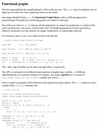
Functional graphsThe best representation for a graph depends a little on the use case. The Graph type in containers uses anadjacency list and a few basic graph operations are provided.

One unique Haskell library, fgl, for Functional Graph Library, takes a different approach toprogramming with graphs, by considering graph as an inductive data-type.

One of the core ideas in fgl is contexts and decomposition. A context of a graph node is a triplet of thenode's predecessors, successors, and the node itself. All graph manipulations can be expressed asinductive recursions over the contexts of a graph. Furthermore, it's surprisingly efficient.

For reference, here's a very, very small section of the fgl API:

-- module Data.Graph.Inductive.Graph

type Adj b = [(b, Node)]

type Context a b = (Adj b, Node, a, Adj b)

type Decomp g a b = (Mcontext a b, g a b)

empty :: Graph gr => gr a bmatch :: Graph gr => Node → gr a b → Decomp gr a b(&) :: DynGraph gr => Context a b → gr a b → gr a b

The a and b type variables are for node and edge labels, respectively.

The API is overloaded over different representations of graphs (type variable gr). Differentimplementations are in distinct modules; for instance, one using a patricia tree is located inData.Graph.Inductive.PatriciaTree module and called Gr a b.

Here's a small toy program which illustrates (de)composition using contexts. The build function createsa graph while sumNodes consumes one:

-- file: fgl.hs

import Data.Graph.Inductive.Graphimport Data.Graph.Inductive.PatriciaTree

build :: Int -> Gr Int ()build 0 = emptybuild n = (to, n, n, from) & build (n - 1) where to = [] from = [ ((), m) | m <- [n - 1, n - 2 .. 0] ]

sumNodes :: [Int] -> Gr Int () -> IntsumNodes [] _ = 0sumNodes (n:ns) gr = case mctx of Nothing -> sumNodes ns gr Just (_,_,x,from) -> x + sumNodes (ns ++ [ m | (_,m) <- from ]) gr'

where (mctx, gr') = match n gr

There are a lot of graph algorithms already implemented in fgl, as well as general combinators to helpbuilding your own special traversals. The feel in the library is very functional indeed: there's no need todrag along the graph or worry about keeping it consistent. In fgl, graphs are immutable, referentiallytransparent, while simultaneously not sacrificing speed.

Numeric data for special useThe libraries in this subsection are as follows:

base (module Data.Fixed): Standard fixed-precision arithmetic from the base. Precision decided atcompile-time.Decimal (module Data.Decimal): Fixed-precision Decimal type and some additional utilityfunctions. Precision decided in runtime.numbers (modules Data.Number.*): Constructive real numbers, multi-precision floats, fixed-precision decimals, and more. Precision decided at compile-time.

The Fixed datatype from base is good for fixed-precision arithmetic when you know the precision atcompile-time. The precision is encoded as a phantom type, so it's not convenient to handle multipleprecisions.

The Decimal library defines a more expressive DecimalRaw type and usually used Decimal synonym:

type Decimal = DecimalRaw Integerdata DecimalRaw I = Decimal{ decimalPlaces :: !Word8, decimalMantissa :: !i }

The exponent is expressed as a Word8, giving at most 255 decimal places. The Decimal libraryautomatically handles multiple precisions in the exponent. The result is always most precise (largestexponent). There are also utility functions such as divide and allocate, that distribute a single decimalinto multiple parts or portions. The parts are guaranteed to always sum to the original decimal.

The numbers library implements some exotic number types. It features floating point numbers witharbitrary, user-defined precision decided at compile-time. Constructive real numbers (full-precisionreals; computation may diverge). Automatic forward differentiated numbers, interval numbers and naturalnumbers.

Encoding and serializationIt's an extremely common need to convert data from one format to another. In Haskell, we often likeworking with Haskell values, because of guarantees of strong-typing and the expressivity of algebraicdatatypes, though data must then be converted to and from Haskell values. Conversions should also befast, because there could be a lot of data.

There are a lot of data formats for different use cases: binary serialization to disk for local storage,efficiently packed formats for transmission over network and formats for interfacing with otherapplications, even users, in APIs and the like. Next, we'll glance at some of the widely used binary andtext serialization libraries.

Binary serialization of Haskell valuesThe libraries in this subsection are as follows:

binary, cereal: Serialization using lazy ByteStrings using automatic or custom binary formatsstore: An even more direct and efficient serialization library from FPComplete

Efficiently serializing Haskell values into binary and back is crucial for performance in manyapplications. Fast serialization is important when handling lots of data, sending it over network or storingit on disk. For example, the performance of a disk cache system is highly dependent on the efficiency ofserialization.

The binary package is a battle-tested, widely used library for serialization. It has a fast throughput andan easy API for adding new serialization instances. Usually, adding new instances by hand for customtypes isn't necessary, because there are already generic serializations defined via GHC.Generics. If theformat is important, however, it's necessary to create your own serialization instance.

The cereal package is more or less equivalent to binary. There are no major differences between theselibraries, other than perhaps slightly different default serialization formats.

The store package is a newcomer in the serialization field from FPComplete. The library released in2016 is in a couple of ways even faster than the already quite fast cereal and binary libraries. First,store avoids bit-swapping on x86: both binary and cereal use big endian for numbers while x86 useslittle-endian. Store uses little endian. Second, store minimizes the number of allocations by allocating acorrectly sized ByteString at once, instead of gradually allocating more space during serialization like isdone in binary and cereal.

The store library has proved its competence benchmarks, showing as much as double the performancein encoding and decoding compared to binary and cereal. store isn't quite so portable as binary. Inparticular, older ARM processors are not supported.

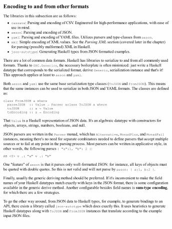
Encoding to and from other formatsThe libraries in this subsection are as follows:

cassava: Parsing and encoding of CSV. Engineered for high-performance applications, with ease ofuse in mind.aeson: Parsing and encoding of JSON.yaml: Parsing and encoding of YAML files. Utilizes parsers and type-classes from aeson.xml: Simple encoding of XML values. See the Parsing XML section (covered later in the chapter)for parsing (possibly malformed) XML in Haskell.json-autotype: Generating Haskell types from JSON formatted examples.

There are a lot of common data formats. Haskell has libraries to serialize to and from all commonly usedformats. Thanks to GHC.Generics, the necessary boilerplate is often minimized: just write a Haskelldatatype that corresponds to the serialized format, derive Generic, serialization instance and that's it!This approach applies at least to aeson and yaml.

Both aeson and yaml use the same base serialization type classes (ToJSON and FromJSON). This meansthat the same instances can be used to serialize in both JSON and YAML formats. The classes are definedas:

class FromJSON a where parseJSON :: Value → Parser aclass ToJSON a where toJSON :: a → Value toEncoding :: a → Encoding

That Value is a Haskell representation of JSON data. It's an algebraic datatype with constructors forobjects, arrays, strings, numbers, booleans, and null.

JSON parsers are written in the Parser monad, which has Alternative, MonadPlus, and MonadFailinstances, meaning there's no need for separate combinators needed to define parsers that accept multiplesources or to fail at any point in the parsing process. Most parsers can be written in applicative style, inother words, the following parses { "a":1, "b": 2 }:

AB <$> v .: "a" v .: "b"

One "feature" of aeson is that it parses only well-formatted JSON: for instance, all keys of objects mustbe quoted with double quotes. So this is not valid and will not parse by aeson: { a:1, b:2 }.

Finally, usually the generic deriving method should be preferred. If it's inconvenient to make the fieldnames of your Haskell datatypes match exactly with keys in the JSON format, there is some configurationavailable in the generic derive method. Another configurable besides field names is sum-type encoding,for which there are a few strategies.

To go the other way around, from JSON data to Haskell types, for example, to generate bindings to anAPI, there exists a library called json-autotype which does exactly this. It uses heuristics to generateHaskell datatypes along with ToJSON and FromJSON instances that translate according to the exampleinput JSON files.

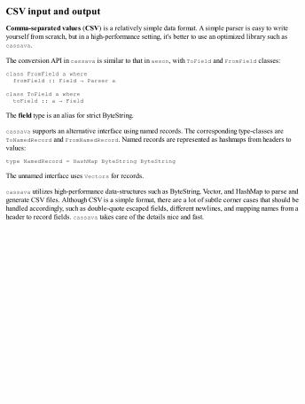
CSV input and outputComma-separated values (CSV) is a relatively simple data format. A simple parser is easy to writeyourself from scratch, but in a high-performance setting, it's better to use an optimized library such ascassava.

The conversion API in cassava is similar to that in aeson, with ToField and FromField classes:

class FromField a where fromField :: Field → Parser a

class ToField a where toField :: a → Field

The field type is an alias for strict ByteString.

cassava supports an alternative interface using named records. The corresponding type-classes areToNamedRecord and FromNamedRecord. Named records are represented as hashmaps from headers tovalues:

type NamedRecord = HashMap ByteString ByteString

The unnamed interface uses Vectors for records.

cassava utilizes high-performance data-structures such as ByteString, Vector, and HashMap to parse andgenerate CSV files. Although CSV is a simple format, there are a lot of subtle corner cases that should behandled accordingly, such as double-quote escaped fields, different newlines, and mapping names from aheader to record fields. cassava takes care of the details nice and fast.

Persistent storage, SQL, and NoSQLThe libraries in this subsection are as follows:

acid-state and safecopy: These libraries go hand in hand, giving a lightweight, disk-storeddatabase of Haskell values with strong ACID guarantees and migrations.persistent: A by-product of the Yesod web framework, persistent is a backend-agnostic high-level query abstraction over SQL-like databases. Provides type-safe models with automatic schemamigrations.esqueleto: Add type-safe SQL query EDSL that works with the persistent library and its models.HDBC: A SQL database abstraction layer similar to persistent except lower level. Providestransactions and marshalling of SQL values to Haskell values and the other way around.HDBC-odbc: Hook any ODBC-enabled database connection to HDBC.persistent-odbc: Hook any ODBC-enabled database connection to persistent via HDBC-odbc.Adds model and migration support.

acid-state and safecopyThe acid-state package provides a very good little database when the database can fit completely inmemory. In short, acid-state uses a Haskell value as the database and user-defined transactions toquery and update the database.

The database is stored in memory and on disk. The disk copy is very resistant to corruption, and call berolled back to any earlier version assuming the event log and a checkpoint is still intact.

The safecopy package extends the cereal binary serialization package with version-controlledformats. It's relatively painless to change the serialization format even deep down in a hierarchy ofdatatypes.

The only downside is that both the old and new format must co-exist in code at least for the time ofmigrating. You are free to rename and move the old datatype freely, though. The only thing that matters isthe version number, which must always increase when schema is changed.

persistent and esqueletoThe persistent library makes it almost trivial to work with SQL and also NoSQL databases fromHaskell. By defining your database models in the embedded model language, persistent generatesstrongly typed model definitions that work with persistent functions to insert, delete, and update rows.Lots of database adapters are available of varying quality, most notably SQLite, PostgreSQL, andMongoDB are well supported.

Here's how we would define a database schema in persistent, using TemplateHaskell and quosi-quoting:

share [mkPersist sqlSettings, mkMigrate "migrateAll"] [persistLowerCase|User username Text UniqueUsername usernamePost author UserId content Text|]

In this schema, we have two tables, user and post. Both will have fields named id automatically. ThatUniqueUsername will turn into two things: a uniqueness constraint in the database and a Haskell data-constructor with which we can query unique rows from the table using getBy function of persistent.

To use this schema with say the SQLite in-memory backend, we could write the following Haskell main:

main = runSqlite ":memory:" $ do -- (1) runMigration migrateAll -- (2)

uid ← insert $ User "foobar" -- (3) insert $ Post uid "First post"

posts ← selectList [PostAuthor ==. uid] -- (4) [Asc PostContent] liftIO $ print $ map (postContent . entityVal) posts

There is nothing that isn't type-safe in this example. At (1), the runSqlite function initializes aconnection to a database and runs an action in it. In case of exceptions, the database is closed cleanly.

At (2), we perform database migrations if necessary. The migrator takes the schema definition as itstarget state, creating new tables and columns when necessary. Note that no destructive actions are takenautomatically; dropping tables and columns must be done manually.

At (3), we perform a simple insertion to the database. The insert function returns the ID of the newlycreated row. We use this ID to consequently add a post entry to the database.

At (4), we use a simple selectList function of persistent to query some rows from the database.Note that persistent intentionally only deals with single tables: it doesn't do joins at all. Joins can bedone either via raw SQL (automatic value interpolation is still provided in raw SQL queries) or with theesqueleto DSL.

Esqueleto is an add-on to persistent that brings complex database queries in a very type-safe embeddeddomain-specific language. Notably, table joins are supported, which is missing from persistent (unlessmanually crafting the query string). Queries in Esqueleto look a lot like queries in SQL, albeit with someextra noise from fancy operator names. A little noise is a small price to pay for compile-time checkedqueries.

For instance, here's an example query written in Esqueleto:

select $from $ \(user `InnerJoin` post) → do on (user ^. UserId ==. post ^. PostAuthor) return (user, post)

This performs an inner join over tables user and post, returning all posts along with their author. It'sequivalent to the following SQL:

SELECT user.* post.*FROM userINNER JOIN post ON user.id = post.author

HDBC and add-onsHDBC is a library older than persistent, and is not as ambitious. HDBC aims to be merely an adapterbetween Haskell and SQL databases.

HDBC works with lots of databases, also including ODBC-compliant databases such as Microsoft SQL.persistent doesn't directly support ODBC, though there is an experimental library called persistent-odbc that adds ODBC compatibility to persistent via HDBC and HDBC-odbc.

HDBC is a better choice than persistent when you don't need automatic migrations, whole modelsupport in Haskell or type-checked queries. HDBC gives just the bare minimum to conveniently interactwith a SQL database from Haskell: connecting to a database, performing queries, and marshalling SQLvalues.

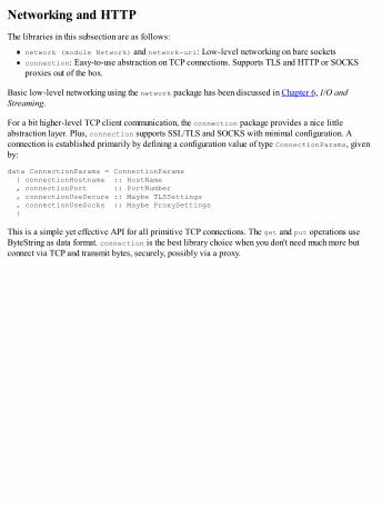
Networking and HTTPThe libraries in this subsection are as follows:

network (module Network) and network-uri: Low-level networking on bare socketsconnection: Easy-to-use abstraction on TCP connections. Supports TLS and HTTP or SOCKSproxies out of the box.

Basic low-level networking using the network package has been discussed in Chapter 6, I/O andStreaming.

For a bit higher-level TCP client communication, the connection package provides a nice littleabstraction layer. Plus, connection supports SSL/TLS and SOCKS with minimal configuration. Aconnection is established primarily by defining a configuration value of type ConnectionParams, givenby:

data ConnectionParams = ConnectionParams { connectionHostname :: HostName , connectionPort :: PortNumber , connectionUseSecure :: Maybe TLSSettings , connectionUseSocks :: Maybe ProxySettings }

This is a simple yet effective API for all primitive TCP connections. The get and put operations useByteString as data format. connection is the best library choice when you don't need much more butconnect via TCP and transmit bytes, securely, possibly via a proxy.

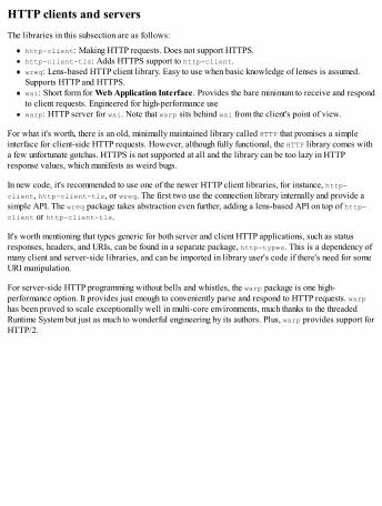
HTTP clients and serversThe libraries in this subsection are as follows:

http-client: Making HTTP requests. Does not support HTTPS.http-client-tls: Adds HTTPS support to http-client.wreq: Lens-based HTTP client library. Easy to use when basic knowledge of lenses is assumed.Supports HTTP and HTTPS.wai: Short form for Web Application Interface. Provides the bare minimum to receive and respondto client requests. Engineered for high-performance usewarp: HTTP server for wai. Note that warp sits behind wai from the client's point of view.

For what it's worth, there is an old, minimally maintained library called HTTP that promises a simpleinterface for client-side HTTP requests. However, although fully functional, the HTTP library comes witha few unfortunate gotchas. HTTPS is not supported at all and the library can be too lazy in HTTPresponse values, which manifests as weird bugs.

In new code, it's recommended to use one of the newer HTTP client libraries, for instance, http-client, http-client-tls, or wreq. The first two use the connection library internally and provide asimple API. The wreq package takes abstraction even further, adding a lens-based API on top of http-client or http-client-tls.

It's worth mentioning that types generic for both server and client HTTP applications, such as statusresponses, headers, and URIs, can be found in a separate package, http-types. This is a dependency ofmany client and server-side libraries, and can be imported in library user's code if there's need for someURI manipulation.

For server-side HTTP programming without bells and whistles, the warp package is one high-performance option. It provides just enough to conveniently parse and respond to HTTP requests. warphas been proved to scale exceptionally well in multi-core environments, much thanks to the threadedRuntime System but just as much to wonderful engineering by its authors. Plus, warp provides support forHTTP/2.

Supplementary HTTP librariesThe libraries in this subsection are as follows:

json-rpc: JSON Remote Procedure Call server and client. Engineered for high performance withease of use in mind. Uses conduits.websockets: Simple web socket server and client library on top of network. Does not supportsecure (WSS) connections.wai-websockets: Uses websockets in a wai (warp) application. Also uses the websocketslibrary. Use this if you already run a wai application and want to add websocket support to it.REST: Can be found on silkapp.github.io/rest. Defining REST APIs in Haskell, with autogenerationof JavaScript client code and documentation.

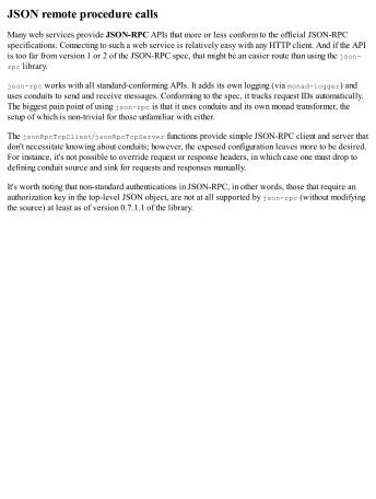
JSON remote procedure callsMany web services provide JSON-RPC APIs that more or less conform to the official JSON-RPCspecifications. Connecting to such a web service is relatively easy with any HTTP client. And if the APIis too far from version 1 or 2 of the JSON-RPC spec, that might be an easier route than using the json-rpc library.

json-rpc works with all standard-conforming APIs. It adds its own logging (via monad-logger) anduses conduits to send and receive messages. Conforming to the spec, it tracks request IDs automatically.The biggest pain point of using json-rpc is that it uses conduits and its own monad transformer, thesetup of which is non-trivial for those unfamiliar with either.

The jsonRpcTcpClient/jsonRpcTcpServer functions provide simple JSON-RPC client and server thatdon't necessitate knowing about conduits; however, the exposed configuration leaves more to be desired.For instance, it's not possible to override request or response headers, in which case one must drop todefining conduit source and sink for requests and responses manually.

It's worth noting that non-standard authentications in JSON-RPC, in other words, those that require anauthorization key in the top-level JSON object, are not at all supported by json-rpc (without modifyingthe source) at least as of version 0.7.1.1 of the library.

Using WebSocketsThe websockets package makes writing WebSocket applications, both client and server, in Haskell abreeze. The API is simple, and the internals are engineered for speed and ease of use. For instance, thereare multiple variants of receive and send functions: for ByteString, Text, and user-defined serializationformats via type-class.

The websockets library is rather flexible, and can be used together with other interfaces. In particular,the wai-websockets library provides a compatibility layer between websockets and wai applications,such as the warp HTTP server. This makes it possible to support both HTTP and upgrading to websockets in the same server application.

Programming a REST APIOne of the most featureful ways to define REST APIs in Haskell is via the Rest framework developed bySilk. See the documentation at http://silkapp.github.io/rest for use. The killer features are automaticgeneration of documentation that's always up-to-date, client-code generation for Haskell and JavaScriptclients, and API versioning.

CryptographyThe libraries in this subsection are as follows:

SHA and RSA: Pure implementations of SHA routines and RSA encryption and signature algorithms.Not the fastest, but plain Haskell without any FFI. Created by Galois Inc.HsOpenSSL: Partial bindings to OpenSSL via FFI.cryptonite: Low-level cryptography primitives with varying API's and probably of varyingquality.skein: Bindings to the skein family of fast and secure cryptographic hash functions.

For really robust, production-ready cryptography applications, one should look for bindings to existingcryptography libraries. For instance, the C implementation of the Skein hash function family has Haskellbindings in the similarly named library skein.

Although Haskell can be used to implement cryptographic algorithms, many of the algorithms rely on bit-twiddling for security in ways that GHC's code optimizations can potentially negate. This makes codevulnerable to side-channel attacks.

That said, some pure Haskell implementations of some algorithms exist. In particular, the RSA package isgood and very suitable when external library dependencies are inconvenient. For what it's worth, the RSApackage is developed at Galois Inc, a known US military contractor.

The cryptonite package provides miscellaneous cryptography building blocks. They are deemedrelatively secure, but every use should be considered individually. There are not too many users orcryptography experts that will have thoroughly reviewed all of the library.

Web technologiesThe libraries in this subsection are as follows:

Yesod framework: Full-blown MVC web framework, with all the bells and whistles.Snap / Happstack: Also web frameworks, independent from each other. Comprises fewer featuresthan Yesod, but still very useful.blaze-html: Blazingly fast combinator library for HTML templating. Uses ByteStrings and thebuilder pattern.amazonka / AWS: Bindings to the Amazon Web Service API. The amazonka bindings areautogenerated, full bindings, while aws is more user-friendly but partial.

Developing full-blown web applications in Haskell is easy, and there are multiple great libraries withoverlapping features. In short, there are three major big frameworks: Yesod, Snap, and Happstack. Eachof these provides basic things such as routing and templating. Yesod has most features of them, but alsothe steepest learning curve.

For just writing HTML in Haskell, one of the best options is blaze-html. blaze-html provides Haskellcombinators for defining HTML. Internally it uses ByteString and builders, to quickly and incrementallygenerate web pages. There are also templating libraries for CSS and JavaScript as well, in particular the"Shakespearean templates" associated to Yesod.

For interfacing web services such as Amazon's, a few libraries exist. Amazon has at least two Haskellbindings: the autogenerated amazonka bindings and partial, more user-friendly aws library. There's alsopackage fb, which provides bindings to the Facebook graph query language API.

Parsing and pretty-printingThe libraries in this subsection are as follows:

parsec: Very featureful, general parser combinator library. Old and poorly maintained. Slower thanattoparsec

attoparsec: Simple and fast parser combinator library. Fewer features than Parsecmegaparsec: A fork of Parsec, well maintained. Extremely flexible. Faster than Parsec butconsiderably slower than Attoparsechappy / alex: Parser combinator libraries aimed towards parsing (programming language)grammars.pcre-heavy: A reasonable regular-expression library.

Parsing is something that Haskell shines at. Applicative and monadic parser interfaces are reallyexpressive. There are many awesome general-purpose parser libraries for Haskell. In general, the choiceshould be between Attoparsec and Megaparsec.

Attoparsec should be preferred as speed is critical; Megaparsec if features are more important.Attoparsec suits best for well-defined file formats, such as serialization. Megaparsec is a better choicewhen dealing with more arbitrarily formatted input.

The learning curve to all parser combinator libraries is rather steep. However, the general ideas are thesame behind them all: using general Applicative/Monad/Alternative interfaces to declarecombinations and options.

Here are some examples of parsing using Megaparsec. First, imports:

> import Text.Megaparsec> import Text.Megaparsec.String

Parsing in applicative style:

> let p = (,,) <$> digitChar <*> (char '.' *> digitChar) <*> (char '-' *> digitChar)

> parseTest p "2.4-6"('2','4','6')

Alternatives between two parsers (using Alternative):

> parseTest (string "a"<|> string "b") "b""b"

Parsing multiple occurrences of same parser:

> parseTest (many (string "a"<|> string "b")) "aababb"["a","a","b","a","b","b"]

Parsing with lookAhead:

> parseTest (manyTill (string "a") (string ";")) "aaaa;b"

["a","a","a","a"]

Lots of high-level parser combinators are available, but they are all just compositions of smaller parts.Such primitives are, for instance, lookAhead, which applies a parser without consuming input, and try,which turns any parser into a backtracking one that acts like it hadn't consumed input when failing.

The Happy and Alex parser libraries, on the other hand, are geared towards parsing grammars. They suitbest for writing parsers for custom domain-specific languages.

Regular expressions in HaskellRegular expressions (regex) are powerful, but they're pretty much write-only. It's an impossibility toreasonably maintain a sufficiently complex regex. Usually, it's a better idea to use a real parsing library,but regexes are still useful, mostly in one-off cases.

There are a few regex libraries for Haskell. One which has rather good reputation is pcre-heavy. It's anextension of pcre-light. Basically, pcre-heavy adds utility functions such as substitions, splits,and so forth. From the name, we can infer that pcre-light supports expressive Perl 5 compatibleregular expressions. Both libraries are also pure Haskell for maximum portability.

pcre-heavy allows for writing regexes using a fine quasi-quoter, and takes in and returns any stringtype: String, Text, and ByteString are all supported without extra overheads.

Parsing XMLThe library in this subsection tagsoup parses arbitrary XML and HTML documents.

A task that comes up from time to time is parsing XML or HTML documents. The unfortunate thing withmany XML and HTML documents is that they're rarely well formatted: missing end tags are just oneexample of ill-formatted HTML.

Tagsoup is one solution for parsing arbitrary data from XML-formatted documents. To some extent, itsupports ill-formatted XML as well. The API is overloaded over source representation data type, via aStringLike class. It supports all of String, strict and lazy ByteString and strict and lazy Text.

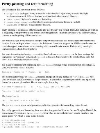
Pretty-printing and text formattingThe libraries in this subsection are as follows:

wl-pprint-* packages: Pretty-printers based on Wadler/Leijen pretty-printers. Multipleimplementations with different features are found in similarly named libraries.text-format: High-performance text formatting.interpolateInterpolate: Simple string interpolation using Template Haskell.here: Docs for Haskell using Template Haskell.

Pretty-printing is the process of turning data into user-friendly text format. Think, for instance, of printinga long string with appropriate line breaks, or printing Haskell values in a friendly way, in other words,commas at the beginning of lines and so on.

The Wadler/Leijen pretty-printer is a simple but powerful interface that has multiple implementations:nearly a dozen packages with wl-pprint in their name. Some add support for ANSI terminal colors, orterminfo support, annotations, one even using a free monad for documents. Unfortunately, no singleimplementation admits for all features.

For basic formatting in classic printf-style, there's of course Text.Printf in the base package thatimplements the "original" polyvariadic printf in Haskell. Unfortunately, it's not at all type-safe. Yetmore, it uses the incredibly slow String.

For high-performance text-formatting, the text-format package brings a formatter for Text values. Atcore, we have the format function:

format :: Params ps => Format → ps → Text

The Format datatype has an IsString instance. Interpolations are marked by "{}". The Params type-class overloads specification styles for parameters. In particular, supported parameters are tuples andlists of parameters, plus others. Here's an example formatting:

> format "testing: {} {} {} {}" (1, 1.23, hex 254, "hello")

"testing: 1 1.23000 fe hello" :: Text

The type of hex is:

hex :: Integral a => a → Builder

The text Builder is also a valid parameter, which is convenient for controlling output format.

For really type-safe text formatting, there are a few interpolation libraries that use Template Haskell forconvenience. For instance, the interpolate library has an almost ludicrously simple interface: onequasi-quoter "i" which is used in this fashion:

> :set -XQuasiQuotes> import Data.String.Interpolate> let world = "World!'> putStrLn [i|Hello #{world} #{9 + 33}|]"Hello World! 42"

However, bear in mind that interpolate uses String as the only possible representation. This can hurtperformance with larger strings. The Here library is similar to interpolate, using different interpolationsyntax (dollar instead of hash) and supporting whitespace trimming.

Control and utility librariesThe libraries in this subsection are as follows:

conduit, io-streams, and pipes: General streaming libraries, that avoid problems with lazy IOlens: Solving the "nested record update" problem in a "batteries included" fashionconvertible: Conversions between types using a single function without information lossbasic-prelude, classy-prelude: Prelude alternatives that encourage best practices in modernHaskellchunked-data: Class abstractions to different builders, zipping, and reading and writing to filesand handles

Streaming libraries are generally aimed at countering problems with lazy IO. Refer to Chapter 6, I/O andStreaming, for an in-depth discussion about problems with lazy IO and Haskell streaming libraries.

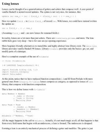
Using lensesLenses can be thought of as a generalization of getters and setters that compose well. A sore point ofvanilla Haskell is nested record updates. The syntax is not very nice, for instance, this:

update rec new_c = rec { field_c = (field_c rec) { c = new_c } }

Here we update field c in field field_c of record rec. With lenses, we could have instead writtenthe update as:

rec & field_c . c .~ new_c

(Assuming field_c and c are now lenses for renamed fields.)

In reality, lenses are a lot more than just setters. There are travelsals, prisms, and more. The lensrabbit hole goes very deep – but is for sure an eye-opening experience.

More beginner-friendly alternatives to monolithic and highly abstract lens library exist. The data-lenslibrary provides vanilla Haskell 98 lenses. Library fclabels provides only the basics: get, set, andmodify parts of a datatype.

Here's a complete example of the use of fclabels:

-- file: fclabels.hs

{-# LANGUAGE TemplateHaskell #-}

import Prelude hiding (id, (.))import Control.Categoryimport Data.Label

At this point, notice that we have replaced function composition (.) and ID from Prelude with moregeneral ones from Category. Fc-lables lenses compose as category, as opposed to lenses of lenslibrary, that compose with function composition.

This is how we define lenses with fc-labels:

data Member = Member { _name :: String , _task :: String } deriving Show

data Team = Team { _leader :: Member , _memebrs :: [Member] } deriving Show

mkLabels [''Member, ''Team]

All the magic happens in the call to mkLabels. Actually, it's not much magic at all; all that happens is thatfrom every field name that begins with an underscore, a lens is formed. The underscore is dropped.

Forming a lens is an entirely mechanical process of defining a getter and modifier. The getter is just

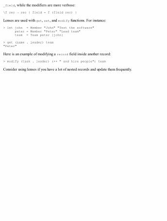
_field, while the modifiers are more verbose:

\f rec → rec { field = f (field rec) }

Lenses are used with get, set, and modify functions. For instance:

> let john = Member "John" "Test the software" peter = Member "Peter" "Lead team" team = Team peter [john]

> get (name . leader) team"Peter"

Here is an example of modifying a record field inside another record:

> modify (task . leader) (++ " and hire people") team

Consider using lenses if you have a lot of nested records and update them frequently.

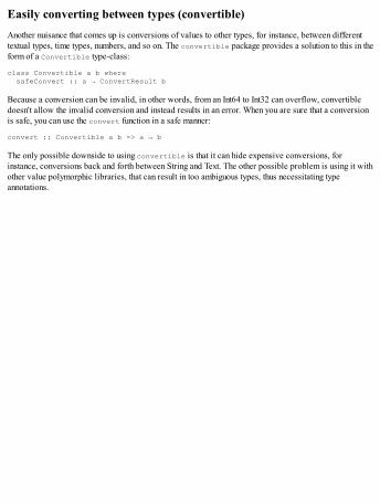
Easily converting between types (convertible)Another nuisance that comes up is conversions of values to other types, for instance, between differenttextual types, time types, numbers, and so on. The convertible package provides a solution to this in theform of a Convertible type-class:

class Convertible a b where safeConvert :: a → ConvertResult b

Because a conversion can be invalid, in other words, from an Int64 to Int32 can overflow, convertibledoesn't allow the invalid conversion and instead results in an error. When you are sure that a conversionis safe, you can use the convert function in a safe manner:

convert :: Convertible a b => a → b

The only possible downside to using convertible is that it can hide expensive conversions, forinstance, conversions back and forth between String and Text. The other possible problem is using it withother value polymorphic libraries, that can result in too ambiguous types, thus necessitating typeannotations.

Using a custom PreludeRelatively advanced Haskellers might find the exports of default Prelude lacking or even devastating:encouraging the use of String, asynchronous exceptions (error), and partial functions. Preferences varyfrom person to person, so in principle there could be as many Preludes as there are Haskellers.

Luckily, one doesn't have to start from scratch defining a custom Prelude, as some better starting pointsexist. The basic-prelude package provides one bare base for building a custom Prelude. The classy-prelude package is aimed at rather advanced programmers, who don't mind working with highly class-based functions.

Some of the convenience classes in classy-prelude come from other smaller packages. For one, themono-traversable library abstracts over monomorphic containers. Essentially, it provides the classesMonoFunctor, MonoFoldable, MonoTraversable, and some others, that are just like Functor,Foldable, and Traversable except that they are monomorphic in the element values. Examples of suchcontainers are Text (element Char) and ByteString (element Word8).

The element type is decided via an open type-family Element:

type family Element mono

Besides truly monomorphic elements, such as Char or Word8, the Element type-family allows forinstances in which the element type is decided from a type variable in the container. For instance, wehave:

type Element [a] = atype Element (Either a b) = b

So the true meaning of "monomorphic" is in the classes, that are less generic than normalFunctor/Foldable/Traversable. For instance, omap of MonoFunctor won't allow changing theelement type unlike fmap would:

omap :: MonoFunctor mono => (Element mono → Element mono) → mono → mono

The motivation for using mono-traversable is that the classes allow for writing generic code thatworks with more container types, in particular using the same code for both monomorphic (Text,ByteString) and polymorphic ([a] and Set a) containers. There are also other type-classes present inthe mono-traversable package; see the package documentation for details.

The chunked-data library was originally a part of classy-prelude, so reasonably it's re-exportedthere. It abstracts over a few things:

Different builders, in particular text and bytestring builders, providing conversions to and frombuilders and their data representationTypes that can be zipped together, in other words, lists, vectors, trees, sequences, and evenIntMaps

The IOData class abstracts over reading and writing Handles

Working with monads and transformersThe libraries in this subsection are as follows:

lifted-base, stm-lifted: Lifting IO operations to arbitrary monad stacksmonad-control: Lifting general control operations to any monad (provides liftBaseWith)monad-logger: Adding high-performance and flexible logging facilities to any monadLogicT: A backtracking logic programming monadmonad-unlift: Provides more reliable state-saving in monad transformer stacks for a subset oftransformers (specifically, monad morphisms)monad-loops: Monad combinators that map, iterate, fold, and unfold with monadic side effects

For choice and considerations of monads and transformers themselves, refer to the discussion in Chapter2, Choose the Correct Data Structures. Logging with monad-logger and fast-logger is discussed in detailin Chapter 6, I/O and Streaming.

Working with monad transformer stacks is most convenient when the actions of used libraries are readilyoverloaded over a type-class that permits use of an arbitrary monad stack. The lifted-base and stm-lifted libraries are alternatives to some base and stm modules. They lift operations from the IO andSTM monad to arbitrary monads overloaded by classes such as MonadIO, MonadBase, andMonadBaseControl.

One monad that hasn't been discussed yet at all is the Logic monad and the LogicT transformer. Thismonad has quite specific use cases: in particular, complex backtracking computations can benefit frombeing written using the Logic monad. It has its own overhead, that's more than, for instance, Maybemonad's overhead in simple cases.

The monad-control package and the MonadBaseControl class are especially useful when writinghighly stateful applications, where nearly all code has to store and have access to resources. Normally,state control operations such as catch live in IO. With liftBaseWith from MonadBaseControl, it'spossible to lift operations that require an IO callback to the custom monad, and allow the callback to runin the custom monad as well. Refer to Chapter 2, Choose the Correct Data Structures for moreinformation about monad-control.

To end our monadic discussion on a lighter note, we note the monad-loops package. It's a package whichadds lots of general but seldom desired monadic operators, such as whileM, iterateWhile, and dozensof other variants. They may or may not make your code more expressive.

Monad morphisms – monad-unliftThe monad-unlift library exists for two reasons:

To allow saving the monadic state (monadic side-effects) in case of an exception. Normally, withliftBaseWith from monad-control, the side-effects are just discarded and there's no way to getthem back if an exception is thrown.As an alternative to monad-control, whose types are extremely general and hard to grasp.

So monad-unlift provides much the same functionality as monad-control, except for a subset ofmonads (transformers). In return, monadic effects can be resurrected in case of an exception. This ispossible for monads that are isomorphic to ReaderT, that is, their effect is not context-sensitive.

In practice, instead of liftBaseWith to run a computation with the saved state, we use askUnliftBaseto get a function that executes actions in the base monad with the same state. The state is shared but mustbe immutable, in other words, the writer part could be represented by a reference.

Handling exceptionsThe libraries in this subsection are as follows:

exceptions: Generalizing extensible extensions to any monad via type-classes (MonadThrow,MonadCatch, and MonadMask)safe-exceptions: At the time of writing, safe-exceptions is a recent attempt at pumping moresense into exception handling in the Haskell ecosystem

When working with custom monads and exceptions, it's advisable to use generalized functions from theexceptions library to conveniently throw, catch, and mask exceptions. The functions work pretty much thesame as their originals from Control.Exception, unless somehow restricted by the base monad.

There are a few nuisances in the way exceptions are handled in Haskell and GHC. In particular,differentiating between synchronous and asynchronous exceptions is fickle. Plus, with current exceptionmechanisms in base, it's easy to make unnecessary mistakes, such as throwing asynchronous exceptionsunintentionally (with throw) or throwing important exceptions away with failing cleanup handlers.

The safe-exceptions package tries to encourage better hygiene with exceptions. It's early indevelopment, so radical changes are still possible. However, it seems prominent enough to include it inthis list.

Random number generatorsThe libraries in this subsection are as follows:

MonadRandom: Simple monadic interface for supplying random numbers. Uses System.Random. It'srather slow and not very secure.mwc-random: Very fast pseudo-random number generation. Probably not cryptographically secure.random-fu: Good support for sampling a wide range of different distributions. Good quality but notterribly slow either.mersenne-random: Pseudo-random numbers using a Mersenne Twister. Probably fastest RNG forHaskell when SIMD is supported.

Random numbers have multiple applications, from simulations to cryptography. Random numbergenerators come with different trade-offs that suit different applications. Others are very fast and notreally that random, while others are slower but cryptographically secure.

Haskell doesn't have a shortage of pseudo-random RNG libraries. Cryptographically secure randomnumbers are hard, however; your best bet is probably in HsOpenSSL or cryptonite.

For pseudo-random number generation, either mwc-random or mersenne-random are good choices. Ifyou need a wider range of distributions and don't mind sacrificing speed, use random-fu.

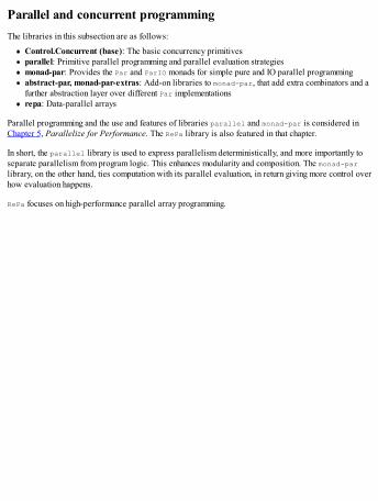
Parallel and concurrent programmingThe libraries in this subsection are as follows:

Control.Concurrent (base): The basic concurrency primitivesparallel: Primitive parallel programming and parallel evaluation strategiesmonad-par: Provides the Par and ParIO monads for simple pure and IO parallel programmingabstract-par, monad-par-extras: Add-on libraries to monad-par, that add extra combinators and afurther abstraction layer over different Par implementationsrepa: Data-parallel arrays

Parallel programming and the use and features of libraries parallel and monad-par is considered inChapter 5, Parallelize for Performance. The RePa library is also featured in that chapter.

In short, the parallel library is used to express parallelism deterministically, and more importantly toseparate parallelism from program logic. This enhances modularity and composition. The monad-parlibrary, on the other hand, ties computation with its parallel evaluation, in return giving more control overhow evaluation happens.

RePa focuses on high-performance parallel array programming.

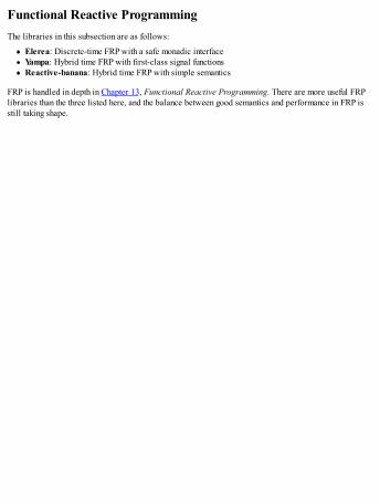
Functional Reactive ProgrammingThe libraries in this subsection are as follows:

Elerea: Discrete-time FRP with a safe monadic interfaceYampa: Hybrid time FRP with first-class signal functionsReactive-banana: Hybrid time FRP with simple semantics

FRP is handled in depth in Chapter 13, Functional Reactive Programming. There are more useful FRPlibraries than the three listed here, and the balance between good semantics and performance in FRP isstill taking shape.

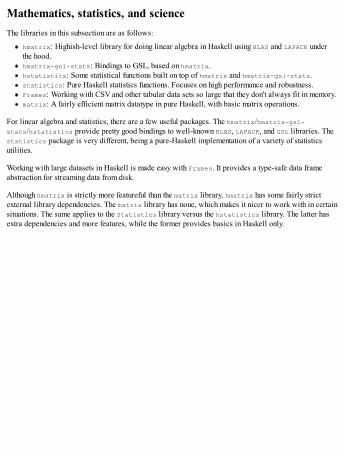
Mathematics, statistics, and scienceThe libraries in this subsection are as follows:

hmatrix: Highish-level library for doing linear algebra in Haskell using BLAS and LAPACK underthe hood.hmatrix-gsl-stats: Bindings to GSL, based on hmatrix.hstatistics: Some statistical functions built on top of hmatrix and hmatrix-gsl-stats.statistics: Pure Haskell statistics functions. Focuses on high performance and robustness.Frames: Working with CSV and other tabular data sets so large that they don't always fit in memory.matrix: A fairly efficient matrix datatype in pure Haskell, with basic matrix operations.

For linear algebra and statistics, there are a few useful packages. The hmatrix/hmatrix-gsl-stats/hstatistics provide pretty good bindings to well-known BLAS, LAPACK, and GSL libraries. Thestatistics package is very different, being a pure-Haskell implementation of a variety of statisticsutilities.

Working with large datasets in Haskell is made easy with Frames. It provides a type-safe data frameabstraction for streaming data from disk.

Although hmatrix is strictly more featureful than the matrix library, hmatrix has some fairly strictexternal library dependencies. The matrix library has none, which makes it nicer to work with in certainsituations. The same applies to the Statistics library versus the hstatistics library. The latter hasextra dependencies and more features, while the former provides basics in Haskell only.

Tools for research and sketchingThe libraries in this subsection are as follows:

ihaskell: Haskell backend for the IPython console and notebook platform.HaTeX: A Haskell EDSL for writing LaTeX documents.H (HaskellR): Embedding R computations into Haskell. Passing data between Haskell and Rwithout copying.

The IPython console and notebook software enable wonderful interactive programming, and ihaskellbrings Haskell to it.

For those who fancy it, writing LaTeX documents is completely possible in Haskell. There is someadded syntactic noise from using an EDSL, but the strong guarantees and high-level abstractions madeavailable by Haskell are worth it in bigger documents. As a plus, HaTeX makes writing TIKZ imagesmuch easier.

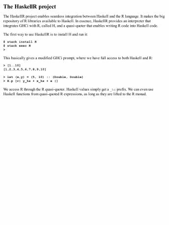
The HaskellR projectThe HaskellR project enables seamless integration between Haskell and the R language. It makes the bigrepository of R libraries available to Haskell. In essence, HaskellR provides an interpreter thatintegrates GHCi with R, called H, and a quasi-quoter that enables writing R code into Haskell code.

The first way to use HaskellR is to install H and run it:

$ stack install H$ stack exec H>

This basically gives a modified GHCi prompt, where we have full access to both Haskell and R:

> [1..10][1,2,3,4,5,6,7,8,9,10]

> let (x,y) = (5, 10) :: (Double, Double)> H.p [r| y_hs + x_hs + e |]

We access R through the R quasi-quoter. Haskell values simply get a _hs prefix. We can even useHaskell functions from quasi-quoted R expressions, as long as they are lifted to the R monad.

Creating charts and diagramsThe libraries in this subsection are as follows:

Chart, Chart-cairo, Chart-diagrams: Rendering 2D charts in Haskell. Supports multiple backends,including Cairo and diagrams.Diagrams: Declaratively generating vector graphics. Supports multiple outputs including Cairo,SVG, PS, and more.

There are two excellent libraries for creating 2D graphics in Haskell: chart and diagrams. The firstone is geared towards charting and plotting, whereas the latter is more on EDSL for generative vectorgraphics.

Both libraries support a wide range of output formats, from vector graphic formats to output directly toGTK windows. Chart even provides some primitive supports for interactivity in charts.

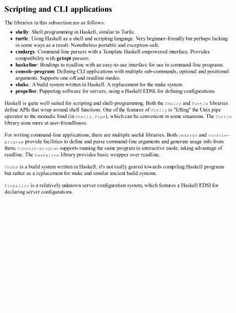
Scripting and CLI applicationsThe libraries in this subsection are as follows:

shelly: Shell programming in Haskell, similar to Turtle.turtle: Using Haskell as a shell and scripting language. Very beginner-friendly but perhaps lackingin some ways as a result. Nonetheless portable and exception-safe.cmdargs: Command-line parsers with a Template Haskell empowered interface. Providescompatibility with getopt parsers.haskeline: Bindings to readline with an easy-to-use interface for use in command-line programs.console-program: Defining CLI applications with multiple sub-commands, optional and positionalarguments. Supports one-off and readline modes.shake: A build system written in Haskell. A replacement for the make system.propellor: Puppeting software for servers, using a Haskell EDSL for defining configurations.

Haskell is quite well suited for scripting and shell-programming. Both the Shelly and Turtle librariesdefine APIs that wrap around shell functions. One of the features of Shelly is "lifting" the Unix pipeoperator to the monadic bind (in Shelly.Pipe), which can be convenient in some situations. The Turtlelibrary aims more at user-friendliness.

For writing command-line applications, there are multiple useful libraries. Both cmdargs and console-program provide facilities to define and parse command-line arguments and generate usage info fromthem. Console-program supports running the same program in interactive mode, taking advantage ofreadline. The haskeline library provides basic wrapper over readline.

Shake is a build system written in Haskell; it's not really geared towards compiling Haskell programsbut rather as a replacement for make and similar ancient build systems.

Propellor is a relatively unknown server configuration system, which features a Haskell EDSl fordeclaring server configurations.

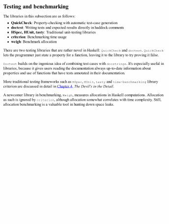
Testing and benchmarkingThe libraries in this subsection are as follows:

QuickCheck: Property-checking with automatic test-case generationdoctest: Writing tests and expected results directly in haddock commentsHSpec, HUnit, tasty: Traditional unit-testing librariescriterion: Benchmarking time usageweigh: Benchmark allocation

There are two testing libraries that are rather novel in Haskell: QuickCheck and doctest. QuickChecklets the programmer just state a property for a function, leaving it to the library to try proving it false.

Doctest builds on the ingenious idea of combining test cases with docstrings. It's especially useful inlibraries, because it gives users reading the documentation always up-to-date information aboutproperties and use of functions that have tests annotated in their documentation.

More traditional testing frameworks such as HSpec, HUnit, tasty and time-benchmarking librarycriterion are discussed in detail in Chapter 4, The Devil's in the Detail.

A newcomer library in benchmarking, Weigh, measures allocations in Haskell computations. Allocationas such is ignored by criterion, although allocation somewhat correlates with time complexity. Still,allocation benchmarking is a valuable tool in hunting down space leaks.

SummaryIn this chapter, we have walked very quickly through a big bunch of libraries in different applicationareas. New libraries are constantly developed, and current ones are being improved. Lists in this chaptershould be taken only as a guideline. It's always a good idea to do a little research before using a newlibrary. The Haskell-Cafe mailing list is a good place to be notified about new libraries and major newreleases, and is relatively low traffic.

During the course of this book, we have navigated many topics that have hopefully helped you become abetter Haskeller.

If you followed closely the first few chapters, you have a good working understanding of lazy evaluationand its traps. You can use seq, bang patterns, and pragmas where necessary. You know many high-performance data structures and are able to use them effectively. In the middle chapters, we learned totest and benchmark, that lazy I/O has drawbacks, to parallelize code, to do concurrency safely and tocompile using appropriate flags for GHC and Runtime System. These are the things that form thefoundation for productive high-performance Haskell programming.

The last topics in this book were more about specific applications of Haskell: interfacing with foreigncode, GPU programming, Cloud Haskell, and functional reactive programming. If you followed throughany of these then you have a good overview of that aspect in Haskell programming and are prepared todive into that subject without friction.

IndexA

aAalex library / Parsing and pretty-printingAattoparsec library / Parsing and pretty-printingabstract-par library / Parallel and concurrent programmingabstract data-types

marshalling / Marshalling abstract datatypesabstract loggers / More abstract loggersAccelerate

matrix multiplication, implementing / Example – Matrix multiplicationAccelerate, concepts

kernels / Kernels – The motivation behind explicit use and runelements / Working with elements and scalarsscalars / Working with elements and scalarsrudimentary array computations / Rudimentary array computationsflow control / Flow control and conditional executionconditional execution / Flow control and conditional executiontuples / Working with tuplesreducing / Folding, reducing, and segmentingsegmenting / Folding, reducing, and segmentingfolding / Folding, reducing, and segmentingstencils / Accelerated stencilspermutation / Permutations in Acceleratebackend foreign function interface / Using the backend foreign function interface

accelerate-cuda package / Running with the CUDA backendAccelerate programs

writing / Writing Accelerate programsgenerated code, inspecting / Inspecting generated code

accumulator parametersabout / Accumulator parameters

accumulatorsabout / Recursion and accumulators

acid-state package / Persistent storage, SQL, and NoSQL, acid-state and safecopyad hoc polymorphic

about / Meeting lazy evaluationaeson library / Encoding to and from other formatsaffinity / Bounded threads and affinityaggressive inlining

about / Inlining and stream fusionAlgebraic Data Types (GADT) / Phantom typesalike package / Pretty-printing and text formattingallocations

minimizing / Increasing sharing and minimizing allocationprofiling / Profiling time and allocations

amazonka Amazonka / Web technologiesanatomy, Haskell project / The anatomy of a Haskell projectarray reductions

via folding / Reduction via foldingarrays

mapping / Mapping and delayed arraysextending / Indices, slicing, and extending arrays

Async APIusing / Using the Async APIexamples, timeouts / Async example – Timeouts

asynchronous errorshandling / Handling asynchronous errors

asynchronous processingabout / Asynchronous processingAsync API, using / Using the Async APIcomposing, with Concurrently type / Composing with Concurrently

attoparsecexample / An example of parsing using io-streams and attoparsec

AWS / Web technologies

Bbase (module Data.Fixed) library / Numeric data for special usebasic-prelude library / Control and utility librariesbenchmarking

about / Benchmarking using the criterion librarywith criterion / Benchmarking using the criterion library

benchmarks / Test suites and benchmarksbidirectional channels

establishing / Establishing bidirectional channelsbinary and textual data, handling

about / Handling binary and textual databit arrays, representing / Representing bit arraysbytes, handling / Handling bytes and blobs of bytesblobs of bytes, handling / Handling bytes and blobs of bytescharacters, working with / Working with characters and stringsstrings, working with / Working with characters and stringsbuilder abstractions, used for iterative construction / Builders for iterative construction

binary I/Oabout / Binary I/O

binary library / Binary serialization of Haskell valuesbinary serialization, libraries

binary / Binary serialization of Haskell valuescereal / Binary serialization of Haskell valuesstore / Binary serialization of Haskell values

binary serialization, of Haskell values / Binary serialization of Haskell valuesbiographical profiling

about / Biographical profilingblaze-html / Web technologiesbounded thread / Bounded threads and affinityboxed types / Heap, stack, and memory managementbranching / Performance of GADTs and branchingbreak-down subset, heap residencies

cost centres (-hc) / Heap profilingper-module (-hm) / Heap profilingclosure descriptions (-hd) / Heap profilingtype description (-hy) / Heap profilingretainers (-hr) / Heap profilingbiography (-hb) / Heap profiling

bufferingabout / File handles, buffering, and encoding

buffering modesBlockBuffering / File handles, buffering, and encodingLineBuffering / File handles, buffering, and encodingNoBuffering / File handles, buffering, and encoding

builder abstractions

using, for iterative construction / Builders for iterative constructionusing, for strings / Builders for strings

ByteString Builder / Builders for iterative constructionbytestring library / Representing data

CC

common types / Common types in Haskell and Ccabal file

fields / Useful fields and flags in cabal filesflags / Useful fields and flags in cabal files

/ Preprocessing Haskell source codecassava library / Encoding to and from other formatscereal library / Binary serialization of Haskell valuesC functions

calling, from Haskell / From Haskell to C and C to HaskellChan

used, for broadcasting / Broadcasting with Chanchannels

using / Using channelscharacters

text library, using / Using the text librarycharts

creating / Creating charts and diagramscharts, libraries

Chart / Creating charts and diagramsChart-cairo / Creating charts and diagramsChart-diagrams / Creating charts and diagrams

chunked-data library / Using a custom PreludechunkedChunked-data library / Control and utility librariesclassy-prelude library / Control and utility librariesclosures / Spawning and closuresCloud Haskell

about / Processes and message-passingcmdargs library / Scripting and CLI applicationsCmm

about / Interpreting GHC's internal representationscode optimizations

state hack / The state hackfloat-in / Floating lets in and outfloat-out / Floating lets in and outcommon subexpressions, eliminating / Eliminating common subexpressionsliberate case duplicates code / Liberate-case duplicates code

Common Subexpression Elimination (CSE) / Eliminating common subexpressionscommon types, C / Common types in Haskell and Ccommon types, Haskell / Common types in Haskell and Ccompiler code optimizations

about / Compiler code optimizationsconcurrency primitives

about / Threads and concurrency primitives

conduit library / Control and utility librariesconnectionConnection library / Networking and HTTPconsole-program / Scripting and CLI applicationsconstant applicative form (CAF)

about / Constant applicative formConstant Applicative Form (CAF) / Setting cost centres manuallycontainers library / Representing dataControl.Concurrent (base) library / Parallel and concurrent programmingcontrol and utility libraries

pipes / Control and utility librariesconduit / Control and utility librariesio-streams / Control and utility librarieslens / Control and utility librariesconvertibleConvertible / Control and utility librariesclassy-prelude / Control and utility librariesbasic-prelude / Control and utility librarieschunkedChunked-data / Control and utility libraries

control inliningabout / Control inliningrewrite rules, using / Using rewrite rulesdefinitions, specializing / Specializing definitionsphase control / Phase control

convertibleConvertible library / Control and utility librariesconvolution operation

with stencils / Convolution with stencilsCore / Using GHC like a procost centre-based heap profiling

about / Cost centre-based heap profilingcost centres

about / Profiling time and allocationssetting, manually / Setting cost centres manuallysetting, automatically / Setting cost centres automatically

C preprocessor (CPP)about / Preprocessing Haskell source codeuse cases / Preprocessing Haskell source code

criterion benchmark suiteabout / Benchmarking using the criterion library

cryptographyabout / Cryptography

cryptography, librariesSHA / CryptographyRSA / CryptographyHsOpenSSL / Cryptographycryptonite / CryptographyskeinSkein / Cryptography

cryptonite package / Cryptography

CSV input / CSV input and outputCSV output / CSV input and outputCUDA backend

using / Running with the CUDA backendCUDA programs

debugging / Debugging CUDA programscustom Prelude

using / Using a custom Prelude

Ddata-type generic programming

about / Datatype generic programminggeneric sum example / Working example – A generic sum

data marshalabout / Data marshal and stable pointers

data parallel programmingabout / Data parallel programming – Repa

data representationlibraries / Representing data

datatype fieldsunpacking / Annotating strictness and unpacking datatype fields

datatype generic programmingabout / Datatype generic programming

debuggingoptions / Options for profiling and debugging

Decimal (module Data.Decimal) library / Numeric data for special usedefinitions

specializing / Specializing definitionsdelayed arrays / Mapping and delayed arraysdelayed representations / Delayed representation and fusiondiagrams

creating / Creating charts and diagramsDiagrams library / Creating charts and diagramsdifference lists

using / Using difference listsperformance / Difference list performanceusing, with writer monad / Difference list with the Writer monad

discrete-time eventsabout / Switching and discrete-time events

domain specific language (DSL)about / Launching missiles during compilation

Eekg

used, for monitoring over HTTP / Monitoring over HTTP with ekgElerea

about / The tiny discrete-time Elereaperformance / Performance and limitations in Elerealimitations / Performance and limitations in Elerea

/ Functional Reactive Programmingencoding / File handles, buffering, and encoding, Encoding and serializationencoding, libraries

cassava / Encoding to and from other formatsaeson / Encoding to and from other formatsyaml / Encoding to and from other formatsxml / Encoding to and from other formatsjson-autotype / Encoding to and from other formats

ephemeral data structuresabout / Ephemeral data structuresmutable references / Mutable references are slowmutable arrays, using / Using mutable arraysmutable vectors, using / Using mutable vectors

erroringabout / Erroring and handling exceptions

errorssynchronous errors, handling / Handling synchronous errorsasynchronous errors, handling / Handling asynchronous errors

esqueleto DSL / persistent and esqueletoesqueleto library / Persistent storage, SQL, and NoSQL, persistent and esqueletoEval monad

about / The Eval monad and strategieseventlog

used, for tracing / Tracing using eventlogevents, and behaviors

combining / Combining events and behaviorsswitching / Switching events and behaviors

examples, from image processingabout / Example from image processingimage, loading from file / Loading the image from fileletters, identifying with convolution / Identifying letters with convolutionstrings, extracting from image / Extracting strings from an imageperformance, testing / Testing and evaluating performanceperformance, evaluating / Testing and evaluating performance

exception hierarchy / The exception hierarchyexceptions

handling / Erroring and handling exceptions, Handling exceptionsexceptions, libraries

exceptionsExceptions / Handling exceptionssafe-exceptions / Handling exceptions

exceptionsExceptions library / Handling exceptions

Ffailure, handling

about / Handling failuremonitors, firing up / Firing up monitorsmatching on message queue / Matching on the message queueprocesses, linking together / Linking processes togethermessage-passing performance / Message-passing performance

file handlesabout / File handles, buffering, and encoding

finger trees / Accessing both ends fast with SeqFlexibleInstances / Useful GHC extensionsforce

using / When in doubt, use the forceformats

encoding to / Encoding to and from other formatsencoding from / Encoding to and from other formats

FP Complete / Using the stack toolFrames library / Mathematics, statistics, and sciencefunctional dependencies

about / Functional dependenciesFunctional Graph Library (fgl) / Functional graphsfunctional graphs / Functional graphsFunctional Reactive Programming, libraries

Elerea / Functional Reactive ProgrammingYampa / Functional Reactive ProgrammingReactive-banana / Functional Reactive Programming

function pointers / Function pointers and wrappersfusion / Delayed representation and fusionfutures

about / spawn for futures and promises

GGADTs

performance / Performance of GADTs and branchinggarbage collector

tuning / Tuning the garbage collectorparallel GC / Parallel GC

general algebraic datatypes / Unbox with UNPACKgetopt parsers / Scripting and CLI applicationsGHC

using, like pro / Using GHC like a prooperating / Operating GHCoperating, circular dependency problem / Circular dependenciescode optimizations, adjusting / Adjusting optimizations and transformationscode transformations, adjusting / Adjusting optimizations and transformationscompiling, via LLVM route / Compiling via the LLVM routeshared libraries, linking / Linking and building shared librariesshared libraries, building / Linking and building shared librariesHaskell source code, preprocessing / Preprocessing Haskell source codetype-safety, enforcing with Safe Haskell / Enforcing type-safety using Safe Haskell

GHC's internal representationsinterpreting / Interpreting GHC's internal representationsGHC Core, reading / Reading GHC CoreSpineless tagless G-machine (STG) / Spineless tagless G-machine

GHC-specific featuresabout / Primitive GHC-specific featureskinds encode type, representation / Kinds encode type representation

GHC Coreconsiderations / Reading GHC Core

GHC extensionsabout / Useful GHC extensionsfor patterns / Extensions for patterns and guardsfor guards / Extensions for patterns and guards

GHCitip / Inspecting time and space usageRepa, working / Playing with Repa in GHCi

GHC optionssummaries / Summary of useful GHC optionsflags / Basic usageLLVM backend / The LLVM backendoptimization, turning on / Turn optimizations on and offoptimization, turning off / Turn optimizations on and offRuntime System (compile-time), configuring / Configuring the Runtime System (compile-time)Safe Haskell compilation, controlling / Safe Haskell

GHC PrimOpscoding in / Coding in GHC PrimOps

GHC Runtime Systemand threads / Runtime System and threadsasynchronous exceptions, masking / Masking asynchronous exceptions

GNU Multiple Precision Arithmetic Library (GMP) / Handling numerical datagranularity

fine-tuning, with chunking / Fine-tune granularity with chunking and bufferingfine-tuning, with buffering / Fine-tune granularity with chunking and buffering

green threads / Scheduler and green threadsguarded recursion

about / Guarded recursion

HH (HaskellR) / Tools for research and sketchingHackage / Running with the CUDA backendHappstack / Web technologieshappy library / Parsing and pretty-printinghashtables library / Representing datahaskelineHaskeline library / Scripting and CLI applicationsHaskell

tests, writing for / Writing tests for Haskellabout / Reading, writing, and handling resourcesevaluation stack, using / Evaluation stack in Haskellgenerating / Generating Haskell with Haskellsplicing, with $(…) / Splicing with $(…)names, in templates / Names in templatessmart template constructor / Smart template constructorsconstN function / The constN functioncode lifting to Q, with quotation brackets / Lifting Haskell code to Q with quotation bracketsmissiles, launching on compilation / Launching missiles during compilationdata, reifying into template objects / Reifying Haskell data into template objectssetters, deriving with Template Haskell / Deriving setters with Template Haskellquasiquoting, for DSLs / Quasi-quoting for DSLscommon types / Common types in Haskell and C

Haskell callbacks, from C / Haskell callbacks from CHaskell functions

exporting / Exporting Haskell functionsHaskell programs

time, inspecting / Inspecting time and space usagespace usage, inspecting / Inspecting time and space usage

Haskell projectanatomy / The anatomy of a Haskell project

HaskellR projectabout / The HaskellR project

HaTeX / Tools for research and sketchingHDBC / Persistent storage, SQL, and NoSQL, HDBC and add-onsHDBC-odbc / Persistent storage, SQL, and NoSQLheap objects, biographical profiling

state LAG / Biographical profilingstate USE / Biographical profilingstate DRAG / Biographical profilingstate VOID / Biographical profiling

heap profilingabout / Heap profilingcost centre-based heap profiling / Cost centre-based heap profiling

here library / Pretty-printing and text formattinghmatrix-gsl-stats library / Mathematics, statistics, and science

hmatrix library / Mathematics, statistics, and sciencehpc command-line utility / Test frameworksHsOpenSSL library / CryptographyHspec

about / Writing tests for Haskell, Test frameworksreference / Test frameworks

hstatistics library / Mathematics, statistics, and sciencehttp-client library / HTTP clients and serversHTTP clients and servers, libraries

http-client / HTTP clients and servershttpHTTP-client-tls / HTTP clients and serverswreq / HTTP clients and serverswai / HTTP clients and serverswarp / HTTP clients and servers

httpHTTP-client-tls library / HTTP clients and serversHUnit

used, for unit testing / Unit testing with HUnit

II/O

lazy I/O / Traps of lazy I/Obinary I/O / Binary I/Otextual I/O / Textual I/Olifting up from / Lifting up from I/Otop-level mutable references / Top-level mutable referenceslifting, from base monad / Lifting from a base monadlifting, base with exception handling / Lifting base with exception handling

I/O performancewith filesystem objects / I/O performance with filesystem objects

ihaskell / Tools for research and sketchingindefinite blocking / Indefinite blocking and weak referencesindices / Indices, slicing, and extending arraysinlining

about / Inlining and stream fusionconsiderations / Inlining and stream fusion

Inter-process Communication (IPC) / Acting as a TCP server (Unix domain sockets)International Components for Unicode (ICU) / Using the text libraryinterpolateInterpolate library / Pretty-printing and text formattingio-streams

example / An example of parsing using io-streams and attoparsecio-streams library / Control and utility libraries

Jjson-autotype library / Encoding to and from other formatsJSON-RPC APIs / JSON remote procedure callsjsonJSON-rpc library / Supplementary HTTP libraries

Llazy evaluation schema

about / Meeting lazy evaluationsum, writing correctly / Writing sum correctlyweak head normal form / Weak head normal formfolds / Folding correctly

lazy I/Oabout / Traps of lazy I/O

lensesusing / Using lenses

lens library / Control and utility librarieslibraries

installing, with profiling / Installing libraries with profilinglibraries, for data representation

vector / Representing datatext / Representing databytestring / Representing datacontainers / Representing dataunordered-containers / Representing datahashtables / Representing datamutable-containers / Representing data

libraries, for mathematicshmatrix / Mathematics, statistics, and sciencehmatrix-gsl-stats / Mathematics, statistics, and sciencematrixMatrix / Mathematics, statistics, and science

libraries, for monads and transformersLifted-base / Working with monads and transformersstm-lifted / Working with monads and transformersMonad-control / Working with monads and transformersMonad-logger / Working with monads and transformersLogicT / Working with monads and transformersmonadMonad-unlift / Working with monads and transformersMonad-loops / Working with monads and transformers

libraries, for parallel and concurrent programmingControl.Concurrent (base) / Parallel and concurrent programmingParallel / Parallel and concurrent programmingmonadMonad-par / Parallel and concurrent programmingmonad-par-extras / Parallel and concurrent programmingabstract-par / Parallel and concurrent programmingrepa / Parallel and concurrent programming

libraries, for parsing and pretty-printingparsec / Parsing and pretty-printingAattoparsec / Parsing and pretty-printingmegaparsec / Parsing and pretty-printinghappy / aAalex / Parsing and pretty-printing

pcre-heavy / Parsing and pretty-printinglibraries, for pretty-printing and text formatting

wl-pprint / Pretty-printing and text formattingalike / Pretty-printing and text formattingtext-format / Pretty-printing and text formattinginterpolateInterpolate / Pretty-printing and text formattinghere / Pretty-printing and text formatting

libraries, for Scripting and CLI applicationsshelly / Scripting and CLI applicationsturtle / Scripting and CLI applicationscmdargs / Scripting and CLI applicationshaskelineHaskeline / Scripting and CLI applicationsconsole-program / Scripting and CLI applicationsshakeShake / Scripting and CLI applicationspropellor / Scripting and CLI applications

libraries, for statisticshstatistics / Mathematics, statistics, and sciencestatistics / Mathematics, statistics, and science

libraries, for testing and benchmarkingQuickCheck / Testing and benchmarkingdoctest / Testing and benchmarkingHSpec / Testing and benchmarkingHUnit / Testing and benchmarkingtasty / Testing and benchmarkingcriterion / Testing and benchmarkingweigh / Testing and benchmarking

libraries, Reparepa-devil / Additional librariesrepa-io / Additional librariesrepa-algorithms / Additional librariesrepa-stream / Additional librariesrepa-flow / Additional libraries

Lifted-base library / Working with monads and transformerslogging, in Haskell

about / Logging in Haskellwith FastLogger / Logging with FastLogger

LogicT library / Working with monads and transformers

MMagicHash language extension / Coding in GHC PrimOpsmanifest representations / Manifest representationsmarshalling

in standard libraries / Marshalling in standard librariesmatrixMatrix library / Mathematics, statistics, and sciencemegaparsec library / Parsing and pretty-printingmemoization

about / Memoization and CAFsmemory

allocating, outside heap / Allocating memory outside the heapmersenne-random library / Random number generatorsMersenne Twister / Random number generatorsmessage-passing

about / Processes and message-passingmessage type

creating / Creating a message typemigrator / persistent and esqueletomodules

Safe / Enforcing type-safety using Safe HaskellSafe-Inferred / Enforcing type-safety using Safe HaskellTrustworthy / Enforcing type-safety using Safe HaskellUnSafe / Enforcing type-safety using Safe Haskell

moments / Reactive-banana – Safe and simple semanticsobserving, on demand / Observing moments on demand

monadworking with / Working with monads and monad stackslist monad / The list monad and its transformertransformer / The list monad and its transformerfree monads / Free monadstransformers, working with / Working with monad transformersspeedup, via continuation-passing style / Speedup via continuation-passing style

Monad-control library / Working with monads and transformersMonad-logger library / Working with monads and transformersMonad-loops library / Working with monads and transformersmonad-par-extras library / Parallel and concurrent programmingmonad-unlift library

need for / Monad morphisms – monad-unliftmonadic loggers

customizing / Customizing monadic loggersmonadic logging / Monadic loggingMonad instance / Reactive-banana – Safe and simple semanticsmonadMonad-par library / Parallel and concurrent programmingmonadMonad-unlift library / Working with monads and transformersMonadRandom library / Random number generators

monadsthrow function, implementing / Throw and catch in other monads besides IOcatch function, implementing / Throw and catch in other monads besides IOworking with / Working with monads and transformers

monad stacksworking with / Working with monads and monad stacks

monad transformer library (mtl) / Working with monad transformersmonitoring

in realtime / Profile and monitor in real timemonitoring, over HTTP

with ekg / Monitoring over HTTP with ekgmonomorphism restriction (MR)

about / Monomorphism Restrictionmulti-package projects / Multi-package projectsMultiParamTypeClasses / Useful GHC extensionsmutable-containers library / Representing datamutable vectors

using / Using mutable vectorsbubble sort, using with / Bubble sort with vectors

mutually recursive signalsabout / Mutually recursive signalsside effects, signalling / Signalling side-effectssignal networks, changing dynamically / Dynamically changing signal networks

MVarsabout / MVarfeatures / MVars are fairused, as building blocks / MVar as a building block

mwc-random library / Random number generators

Nnetwork (module Network) library / Networking and HTTPnetwork-transport library

about / Networking above the transport layernetwork-uri library / Networking and HTTPnetworking

about / Sockets and networkingabove transport layer / Networking above the transport layer

/ Nodes and networkingnetworking and HTTP, libraries

network (module Network) / Networking and HTTPnetwork-uri / Networking and HTTPconnectionConnection / Networking and HTTP

nodes / Nodes and networkingNoMonomorphismRestriction language extension

about / Monomorphism Restrictionnon-deterministic parallelism

with ParIO / Non-deterministic parallelism with ParIONormal Form (NF) / Weak head normal form, When in doubt, use the forceNormal Form Data (NFData) / Benchmarking using the criterion librarynumbers (modules Data.Number.*) library / Numeric data for special usenumerical data

handling / Handling numerical datanumeric data, libraries

base (module Data.Fixed) / Numeric data for special useDecimal (module Data.Decimal) / Numeric data for special usenumbers (modules Data.Number.*) / Numeric data for special use

numeric types, Haskell / Handling numerical data

OO(log n) / Using the containers packageobjects

outside heap / Objects outside the heappointing, in heap / Pointing to objects in the heap

Operating System (OS) thread / Threads and mutable references

Pparallelism

diagnosing / Diagnosing parallelism – ThreadScopeParallel library / Parallel and concurrent programmingParIO

using, for non-deterministic parallelism / Non-deterministic parallelism with ParIOPar monad

about / The Par monad and schedulesparsec library / Parsing and pretty-printingparsing

about / Parsing and pretty-printingpartial functions

about / Partial functionspartitioned arrays

about / Cursored and partitioned arrayspatricia / Functional graphsPatternGuards

about / Extensions for patterns and guardsPatternSynonyms

about / Extensions for patterns and guardspcre-heavy library / Parsing and pretty-printingPerl 5 compatible regular expressions / Regular expressions in Haskellpersistent-odbc / Persistent storage, SQL, and NoSQLpersistent library / Persistent storage, SQL, and NoSQL, persistent and esqueletophantom types

about / Phantom typespipes

benefits / Strengths and weaknesses of pipesdrawbacks / Strengths and weaknesses of pipes

pipes library / Control and utility librariespolymorphic

about / Meeting lazy evaluationpolymorphic programs / Polymorphism performancepolymorphism performance / Polymorphism performancepretty-printing / Pretty-printing and text formattingprimitive parallelism

about / Primitive parallelism and the Runtime Systemprocesses

about / Processes and message-passingcreating / Creating a Process

profilerunexpected crashes, debugging with / Debugging unexpected crashes with profiler

profilingabout / Profiling time and allocationslibraries, installing with / Installing libraries with profiling

in realtime / Profile and monitor in real timeoptions / Options for profiling and debugging

promisesabout / spawn for futures and promises

propellor library / Scripting and CLI applicationsproperty checks

about / Property checkspseq

about / Subtle evaluation – pseq

QQuickCheck

about / Writing tests for Haskell

Rrandom-fu library / Random number generatorsrandom number generators

about / Random number generatorsrandom number generators, libraries

MonadRandom / Random number generatorsmwc-random / Random number generatorsrandom-fu / Random number generatorsmersenne-random / Random number generators

raw UDP trafficabout / Raw UDP traffic

reactimateused, for performing output from network / Reactimate output

Reactive-banana / Reactive-banana – Safe and simple semanticsfirst GUI application / Example – First GUI applicationgraphical display, with wxWidgets / Graphical display with wxWidgetsinput, adding / Adding input and outputoutput, adding / Adding input and outputinput, adding via polling / Input via polling or handlersinput, adding via handlers / Input via polling or handlersinput, adding dynamically / Input and output dynamicallyoutput, adding dynamically / Input and output dynamically

reactive-banana / Functional Reactive ProgrammingReader / Working with monads and monad stacksReader Writer State (RWS) / Working with monad transformersrecursion

about / Recursion and accumulators, Recursion and semanticsregular expressions, in Haskell

about / Regular expressions in Haskellremote process

calling / Calling a remote processRepa

about / Data parallel programming – Repaworking with / Playing with Repa in GHCi

repa-algorithms libraryabout / Additional libraries

repa-devil libraryabout / Additional libraries

repa-flow libraryabout / Additional libraries

repa-io libraryabout / Additional libraries

repa-stream libraryabout / Additional libraries

Repa code

writing / Writing fast Repa coderepa library / Parallel and concurrent programmingresources

reading / Reading, writing, and handling resourceswriting / Reading, writing, and handling resourceshandling / Reading, writing, and handling resourcesmanging, with ResourceT / Managing resources with ResourceT

ResourceTresources, managing with / Managing resources with ResourceT

REST APIprogramming / Programming a REST API

Rest framework, Silkreference / Programming a REST API

Rest REST library / Supplementary HTTP librariesretainer profiling

about / Retainer profilingreverse polish notation (RPN)

about / Guarded recursionrewrite rules

using / Using rewrite rulesRSA library / CryptographyRSpec

about / Test frameworksRTS options

summaries / Summary of useful RTS optionsscheduler flags / Scheduler flagsmemory management / Memory managementgarbage collection / Garbage collectionruntime system statistics / Runtime System statisticsprofiling / Profiling and debuggingdebugging / Profiling and debugging

runtime systemabout / Primitive parallelism and the Runtime System

runtime system, GHCtuning / Tuning GHC's Runtime Systemscheduler threads / Scheduler and green threadsgreen threads / Scheduler and green threadsheap management / Heap, stack, and memory managementstack management / Heap, stack, and memory managementmemory management / Heap, stack, and memory managementgarbage collector, tuning / Tuning the garbage collectortracing options / Profiling and tracing optionsprofiling options / Profiling and tracing options

Ssafe-exceptions library / Handling exceptionssafe-exceptions package / Handling exceptionssafecopy package / Persistent storage, SQL, and NoSQL, acid-state and safecopyschedules

about / The Par monad and schedulesScopedTypeVariables

about / Extensions for patterns and guardssemantics

about / Recursion and semanticsSeq / Accessing both ends fast with Seqsequential data, handling

about / Handling sequential datadifference lists, using / Using difference listszippers, using / Using zippers

serialization / Encoding and serializationSet Cost Centre (SCC) / Setting cost centres manually, Debugging unexpected crashes with profilershakeShake library / Scripting and CLI applicationsSHA library / Cryptographyshared library

compiling / Compiling a shared librarysharing

increasing / Increasing sharing and minimizing allocationShelly library / Scripting and CLI applicationsshelly library / Scripting and CLI applicationssignal functions

state, adding to / Adding state to signal functionsSimpleLocalNet backend

running with / Running with the SimpleLocalNet backendSingle Instruction, Multiple Data (SIMD) / Compiling via the LLVM route

about / Primitive GHC-specific featuresskeinSkein library / Cryptographyslicing / Indices, slicing, and extending arraysSmallCheck

about / Writing tests for Haskellsmap

about / Cursored and partitioned arraysSnap / Web technologiessockets

about / Sockets and networkingSoftware Transactional Memory (STM)

about / Software Transactional Memorybank account example / STM example – Bank accountsalternative transactions / Alternative transactionsexceptions / Exceptions in STM

spark / Sparks and spark poolspark pool

overflowed / Spark awaydud / Spark awayGC'd / Spark awayfizzled / Spark away

/ Sparks and spark poolsparks

about / Spark awaysparse data, handling

about / Handling sparse datacontainers package, using / Using the containers packageunordered-containers package, using / Using the unordered-containers package

spawn functionfor futures / spawn for futures and promisesfor promises / spawn for futures and promises

spawning / Spawning and closuresspec testing

about / Writing tests for HaskellSpineless tagless G-machine (STG)

about / Interpreting GHC's internal representations, Spineless tagless G-machineSpineless Tagless G-machine (STG) / Using GHC like a prostable pointers

about / Data marshal and stable pointersstack manual

reference / Using the stack toolstack tool

using / Using the stack toolstate

adding, to signal functions / Adding state to signal functionsstatic addresses

importing / Importing static functions and addressesstatic functions

importing / Importing static functions and addressesstatistics library / Mathematics, statistics, and sciencestm-lifted library / Working with monads and transformersstore library / Binary serialization of Haskell valuesstrategies

about / The Eval monad and strategiesworking / The Eval monad and strategiescomposing / Composing strategies

stream fusionabout / Inlining and stream fusion

/ Using the text librarystreaming

about / Streaming with side-effects

streaming, with conduitsabout / Streaming using conduitsresources, handling / Handling resources and exceptions in conduitsexceptions, handling / Handling resources and exceptions in conduitsconduits, resuming / Resuming conduits

streaming, with io-streamsabout / Simple streaming using io-streamsinput streams, creating / Creating input streamscombinators, using / Using combinators and output streamsoutput streams, using / Using combinators and output streamsexceptions, handling / Handling exceptions and resources in streamsresources, handling / Handling exceptions and resources in streams

streaming, with pipesabout / Streaming using pipespipes, composing / Composing and executing pipespipes, executing / Composing and executing pipesfor-loops / For loops and category theory in pipescategory theory / For loops and category theory in pipesexceptions, handling / Handling exceptions in pipes

streaming libraryselecting / Choosing a streaming library

stream monad / The list monad and its transformerStrictData

about / Strict-by-default Haskellstrictness

annotating / Annotating strictness and unpacking datatype fieldsstrings

text library, using / Using the text librarysubtle evaluation

with pseq / Subtle evaluation – pseqsum-type encoding / Encoding to and from other formatssupplementary HTTP libraries

jsonJSON-rpc / Supplementary HTTP librarieswebsocketsWebsockets / Supplementary HTTP librarieswai-websockets / Supplementary HTTP librariesRest REST / Supplementary HTTP libraries

switchingabout / Switching and discrete-time events

synchronous errorshandling / Handling synchronous errors

szipWithabout / Cursored and partitioned arrays

Ttabular data, handling

about / Handling tabular datavector package, using / Using the vector package

Tagsoup / Parsing XMLTasty

about / Test frameworksreference / Test frameworks

TCP/IP clientacting as / Acting as a TCP/IP client

TCP serveracting as / Acting as a TCP server (Unix domain sockets)

Template Haskellused, for deriving setters / Deriving setters with Template Haskell

test frameworksabout / Test frameworksHspec / Test frameworksRSpec / Test frameworks

testswriting, for Haskell / Writing tests for Haskell

test suites / Test suites and benchmarkstext-format library / Pretty-printing and text formattingtext formatting / Pretty-printing and text formattingtext library / Representing datatextual I/O

about / Textual I/Othreads

about / Threads and concurrency primitivesand mutable references / Threads and mutable referencesthunk accumulation, avoiding / Avoid accumulating thunksatomic operations, performing with IORefs / Atomic operations with IORefs

ThreadScopeabout / Diagnosing parallelism – ThreadScope

/ Linking and building shared libraries, Tracing using eventlogThread State Objects (TSOs) / Scheduler and green threadstime

profiling / Profiling time and allocationsworking with / Working with time

timed log messages / Timed log messagestools, for research and sketching

ihaskell / Tools for research and sketchingHaTeX / Tools for research and sketchingH (HaskellR) / Tools for research and sketching

tracingeventlog, using / Tracing using eventlog

transformersworking with / Working with monads and transformers

Trivia, at term-levelabout / Trivia at term-levelcoding, in GHC PrimOps / Coding in GHC PrimOpscontrol inlining / Control inlining

Trivia, at type-levelabout / Trivia at type-levelphantom types / Phantom typesfunctional dependencies / Functional dependenciesassociated types / Type families and associated typestype families / Type families and associated types

turtle library / Scripting and CLI applicationsTurtle library / Scripting and CLI applicationsTypeFamilies / Useful GHC extensionstypes

converting between / Easily converting between types (convertible)

UUnboxedTuples extension / Coding in GHC PrimOpsunboxing

about / Unbox with UNPACKanonymous tuples, using / Using anonymous tuples

unexpected crashesdebugging, with profiler / Debugging unexpected crashes with profiler

Unicode-correct / Working with characters and stringsunit testing

with HUnit / Unit testing with HUnitunordered-containers library / Representing dataUNPACK

used, for unboxing / Unbox with UNPACK

Vvector library / Representing dataViewPatterns

about / Extensions for patterns and guards

Wwai-websockets library / Supplementary HTTP librarieswai library / HTTP clients and serverswarp HTTP server

about / Using WebSocketswarp library / HTTP clients and serversWeak Head Normal Form / Benchmarking using the criterion libraryWeak Head Normal Form (WHNF) / Weak head normal formweak references / Indefinite blocking and weak referencesWeak ThreadId / Indefinite blocking and weak referencesWeb Application Interface / HTTP clients and serversWebSocket applications

about / Using WebSocketsWebSockets

using / Using WebSocketswebsocketsWebsockets library / Supplementary HTTP librariesweb technologies

about / Web technologiesweb technologies, libraries

Yesod framework / Web technologiesSnap / Happstack / Web technologiesblaze-html / Web technologiesamazonka Amazonka/ AWS / Web technologies

windowing function / Using the vector packagewl-pprint package / Pretty-printing and text formattingworker/wrapper transformation

about / The worker/wrapper idiomwrappers / Function pointers and wrapperswreq library / HTTP clients and serversWriter / Working with monads and monad stacks

XXML

parsing / Parsing XMLxml library / Encoding to and from other formats

Yyaml library / Encoding to and from other formatsYampa

about / Events and signal functions with Yampasignal functions / Events and signal functions with Yampaevents / Events and signal functions with Yampaintegrating, to real world / Integrating to the real world

/ Functional Reactive ProgrammingYesod framework / Web technologiesYesod web framework / Persistent storage, SQL, and NoSQL

Zzippers

using / Using zippersboth ends, accessing with Seq / Accessing both ends fast with Seq