Heat Transfer Analysis in Wire Bundles for

Aerospace Vehicles

S. L. Rickman, C. J. Iannello NASA Engineering and Safety Center, United States of America

Abstract

Design of wiring for aerospace vehicles relies on an understanding of “ampacity”

which refers to the current carrying capacity of wires, either, individually or in

wire bundles. Designers rely on standards to derate allowable current flow to

prevent exceedance of wire temperature limits due to resistive heat dissipation

within the wires or wire bundles. These standards often add considerable margin

and are based on empirical data. Commercial providers are taking an aggressive

approach to wire sizing which challenges the conventional wisdom of the

established standards. Thermal modelling of wire bundles may offer significant

mass reduction in a system if the technique can be generalized to produce reliable

temperature predictions for arbitrary bundle configurations. Thermal analysis has

been applied to the problem of wire bundles wherein any or all of the wires within

the bundle may carry current. Wire bundles present analytical challenges because

the heat transfer path from conductors internal to the bundle is tortuous, relying

on internal radiation and thermal interface conductance to move the heat from

within the bundle to the external jacket where it can be carried away by convective

and radiative heat transfer. The problem is further complicated by the dependence

of wire electrical resistivity on temperature. Reduced heat transfer out of the

bundle leads to higher conductor temperatures and, hence, increased resistive heat

dissipation. Development of a generalized wire bundle thermal model is presented

and compared with test data. The steady state heat balance for a single wire is

derived and extended to the bundle configuration. The generalized model includes

the effects of temperature varying resistance, internal radiation and thermal

interface conductance, external radiation and temperature varying convective

relief from the free surface. The sensitivity of the response to uncertainties in key

model parameters is explored using Monte Carlo analysis.

Keywords: Ampacity, cable harness, AS50881, wire bundle, thermal analysis

https://ntrs.nasa.gov/search.jsp?R=20160011474 2020-04-02T22:19:03+00:00Z

1 Introduction

Standard practice for cable derating within NASA programs has its roots in test

data collected by the US military, the aviation industry, the Society for Automotive

Engineers (SAE), and at NASA centers and traces back to the 1940s[1-3]. While

these data were thoughtfully collected, documented and re-verified by subsequent

studies, the resulting wire harness derating procedure still included significant

conservatism [1-3]. There are many reasons for this added margin with the most

significant contributor being the need to standardize a simple procedure that

completely enveloped the envisioned use case and resulted in a capable design.

Variables like total harness loading (i.e., load distribution), ambient temperature,

cable construction, conductor alloys, insulation types, etc. are assumed to be

consistent with the test conditions in the wire derating studies and formed the basis

for the derating curves. Changes to these assumptions can have a significant effect

on the ampacity of conductors within the harness allowing for larger margin than

what is predicted by the curves. However, reclaiming this unaccounted for margin

adds complexity to the analysis and added complexity generally runs counter to

the derating procedure’s primary goal which is safe design with an element of ease

of use. In some of NASA’s earliest references on standardizing wire harness

design, the issue of a “one size fits all” wire harness derating was debated and

lamented. [1].

The problem of wire and wire bundle analysis has been studied by van Benthem

et al [4] and Ilgevičius and Liess [5]. Reference 4 focuses on thermal analysis of

wire bundle configurations and highlights the complexity of the analysis by noting

the numerous parameters involved. Reference 5 discusses thermal analysis of

wires using a finite volume method and highlights the complexities involved with

variable parameters and considered non-linear thermal conduction, convection and

radiation as well as temperature varying electrical resistance in a single wire.

This paper seeks to address this longstanding issue via the use of a generalized

model that considers key aspects of the harness design and use case that the current

derating procedure does not fully consider such as insulation type and thickness,

varying ambient temperatures, different conductor materials, various bundle

loading configurations, mixed wire sizes and types in bundles, and more accurate

vacuum prediction. Development of a single wire thermal model is presented and

is extended to that of a bundle configuration. The model includes wire-to-wire

heat conduction and radiation, the effect of temperature-varying resistance as well

as external convection and radiation. The bundle model was easily implemented

as a spreadsheet and can be used to solve steady state problems composed of up

to fifty elements. A Monte Carlo capability has been implemented allowing

exploration of problem sensitivity to, up to six variables.

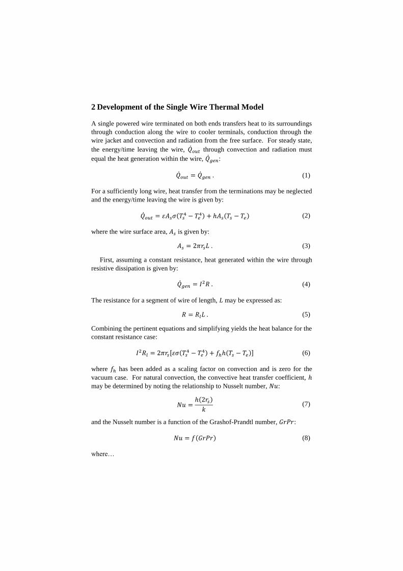
2 Development of the Single Wire Thermal Model

A single powered wire terminated on both ends transfers heat to its surroundings

through conduction along the wire to cooler terminals, conduction through the

wire jacket and convection and radiation from the free surface. For steady state,

the energy/time leaving the wire, �̇�𝑜𝑢𝑡 through convection and radiation must

equal the heat generation within the wire, �̇�𝑔𝑒𝑛:

�̇�𝑜𝑢𝑡 = �̇�𝑔𝑒𝑛 . (1)

For a sufficiently long wire, heat transfer from the terminations may be neglected

and the energy/time leaving the wire is given by:

�̇�𝑜𝑢𝑡 = 𝜀𝐴𝑠𝜎(𝑇𝑠4 − 𝑇𝑒

4) + ℎ𝐴𝑠(𝑇𝑠 − 𝑇𝑒) (2)

where the wire surface area, 𝐴𝑠 is given by:

𝐴𝑠 = 2𝜋𝑟𝑠𝐿 . (3)

First, assuming a constant resistance, heat generated within the wire through

resistive dissipation is given by:

�̇�𝑔𝑒𝑛 = 𝐼2𝑅 . (4)

The resistance for a segment of wire of length, 𝐿 may be expressed as:

𝑅 = 𝑅𝑙𝐿 . (5)

Combining the pertinent equations and simplifying yields the heat balance for the

constant resistance case:

𝐼2𝑅𝑙 = 2𝜋𝑟𝑠[𝜀𝜎(𝑇𝑠4 − 𝑇𝑒

4) + 𝑓ℎℎ(𝑇𝑠 − 𝑇𝑒)] (6)

where 𝑓ℎ has been added as a scaling factor on convection and is zero for the

vacuum case. For natural convection, the convective heat transfer coefficient, ℎ

may be determined by noting the relationship to Nusselt number, 𝑁𝑢:

𝑁𝑢 =ℎ(2𝑟𝑠)

𝑘 (7)

and the Nusselt number is a function of the Grashof-Prandtl number, 𝐺𝑟𝑃𝑟:

𝑁𝑢 = 𝑓(𝐺𝑟𝑃𝑟) (8)

where…

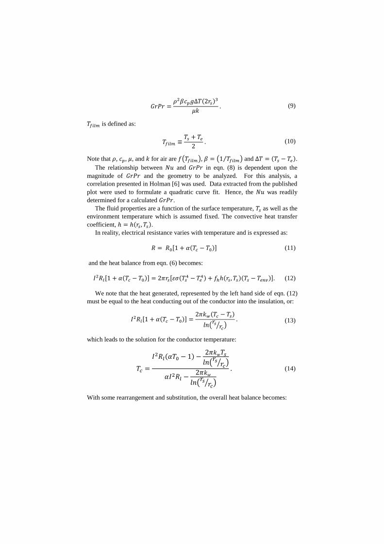
𝐺𝑟𝑃𝑟 =𝜌2𝛽𝑐𝑝𝑔Δ𝑇(2𝑟𝑠)

3

𝜇𝑘 . (9)

𝑇𝑓𝑖𝑙𝑚 is defined as:

𝑇𝑓𝑖𝑙𝑚 ≡𝑇𝑠 + 𝑇𝑒2

. (10)

Note that 𝜌, 𝑐𝑝, 𝜇, and 𝑘 for air are 𝑓(𝑇𝑓𝑖𝑙𝑚), 𝛽 = (1 𝑇𝑓𝑖𝑙𝑚⁄ ) and Δ𝑇 = (𝑇𝑠 − 𝑇𝑒).

The relationship between 𝑁𝑢 and 𝐺𝑟𝑃𝑟 in eqn. (8) is dependent upon the

magnitude of 𝐺𝑟𝑃𝑟 and the geometry to be analyzed. For this analysis, a

correlation presented in Holman [6] was used. Data extracted from the published

plot were used to formulate a quadratic curve fit. Hence, the 𝑁𝑢 was readily

determined for a calculated 𝐺𝑟𝑃𝑟.

The fluid properties are a function of the surface temperature, 𝑇𝑠 as well as the

environment temperature which is assumed fixed. The convective heat transfer

coefficient, ℎ = ℎ(𝑟𝑠 , 𝑇𝑠).

In reality, electrical resistance varies with temperature and is expressed as:

𝑅 = 𝑅0[1 + 𝛼(𝑇𝑐 − 𝑇0)] (11)

and the heat balance from eqn. (6) becomes:

𝐼2𝑅𝑙[1 + 𝛼(𝑇𝑐 − 𝑇0)] = 2𝜋𝑟𝑠[𝜀𝜎(𝑇𝑠4 − 𝑇𝑒

4) + 𝑓ℎℎ(𝑟𝑠, 𝑇𝑠)(𝑇𝑠 − 𝑇𝑒𝑛𝑣)]. (12)

We note that the heat generated, represented by the left hand side of eqn. (12)

must be equal to the heat conducting out of the conductor into the insulation, or:

𝐼2𝑅𝑙[1 + 𝛼(𝑇𝑐 − 𝑇0)] =2𝜋𝑘𝑤(𝑇𝑐 − 𝑇𝑠)

𝑙𝑛(𝑟𝑠𝑟𝑐⁄ )

. (13)

which leads to the solution for the conductor temperature:

𝑇𝑐 =

𝐼2𝑅𝑙(𝛼𝑇0 − 1) −2𝜋𝑘𝑤𝑇𝑠𝑙𝑛(𝑟𝑠𝑟𝑐⁄ )

𝛼𝐼2𝑅𝑙 −2𝜋𝑘𝑤

𝑙𝑛(𝑟𝑠𝑟𝑐⁄ )

. (14)

With some rearrangement and substitution, the overall heat balance becomes:

𝐼2𝑅𝑙 {1 + 𝛼 [𝐼2𝑅𝑙(𝛼𝑇0 − 1) −

2𝜋𝑘𝑤𝑇𝑠𝑙𝑛(𝑟𝑠 𝑟𝑐⁄ )

𝛼𝐼2𝑅𝑙 −2𝜋𝑘𝑤

𝑙𝑛(𝑟𝑠 𝑟𝑐⁄ )

− 𝑇0]}

= 2𝜋𝑟𝑠[𝜀𝜎(𝑇𝑠4 − 𝑇𝑒

4) + 𝑓ℎℎ(𝑟𝑠 , 𝑇𝑠)(𝑇𝑠 − 𝑇𝑒)] .

(15)

Once eqn. (15) is solved iteratively for 𝑇𝑠, eqn. (14) may be used to determine

𝑇𝑐.

3 Development of the Wire Bundle Thermal Model

The single wire heat balance may be extended to represent a collection of wires

into a wire bundle. For the purpose of this analysis, it is assumed that adjacent

conductors may transfer heat to one another via radiation and contact conductance.

In this treatment, no internal convection is assumed. The collection of wires is

assumed to be wrapped in an outer jacket which can exchange heat with the

environment via convection and radiation. For model simplification, only

conduction between the wires and the outer jacket is assumed.

The overall heat transfer between wires within the bundle is represented by the

following system of equations:

(𝐼2𝑅𝑙)𝑖{1 + 𝛼𝑖[(𝑇𝑐)𝑖 − 𝑇0]}

=∑𝐶𝑖𝑗{2𝜋(𝑟𝑠)𝑖𝜀𝑖𝐵𝑖𝑗𝜎[(𝑇𝑠4)𝑖 − (𝑇𝑠

4)𝑗]

𝑛

𝑗=1

+ (𝐺𝑖𝑛𝑡)𝑖𝑗[(𝑇𝑠)𝑖 − (𝑇𝑠)𝑗]}

(16)

where the factor 𝐶𝑖𝑗 is unity when conductors 𝑖 and 𝑗 are adjacent to one another

and zero otherwise. Note also that 𝐶𝑖𝑗 = 0 when 𝑖 = 𝑗. The radiation interchange

factor, 𝐵𝑖𝑗 is pre-computed using an external program for parallel cylinders of

infinite extent in contact, spanning the range of radius ratios and surface optical

properties and referenced as a look-up table as the model is formulated.

Ultimately, the solution to a system of linear equations is sought. However,

the inclusion of thermal radiation poses a problem due to its highly non-linear

nature. To resolve this problem, the radiation terms are linearized by noting:

2𝜋(𝑟𝑠)𝑖𝜀𝑖𝐵𝑖𝑗𝜎[(𝑇𝑠4)𝑖 − (𝑇𝑠

4)𝑗]

= 2𝜋(𝑟𝑠)𝑖𝜀𝑖𝐵𝑖𝑗𝜎[(𝑇𝑠2)𝑖 + (𝑇𝑠

2)𝑗][(𝑇𝑠)𝑖 + (𝑇𝑠)𝑗][(𝑇𝑠)𝑖 − (𝑇𝑠)𝑗]

= (𝐺𝑟𝑎𝑑)𝑖𝑗[(𝑇𝑠)𝑖 − (𝑇𝑠)𝑗]

(17)

where the linearized radiation conductor, (𝐺𝑟𝑎𝑑)𝑖𝑗 = 2𝜋(𝑟𝑠)𝑖𝜀𝑖𝐵𝑖𝑗𝜎[(𝑇𝑠2)𝑖 +

(𝑇𝑠2)𝑗][(𝑇𝑠)𝑖 + (𝑇𝑠)𝑗]. The overall heat balance becomes:

(𝐼2𝑅𝑙)𝑖{1 + 𝛼𝑖[(𝑇𝑐)𝑖 − 𝑇0]}

=∑𝐶𝑖𝑗{(𝐺𝑟𝑎𝑑)𝑖𝑗[(𝑇𝑠)𝑖 − (𝑇𝑠)𝑗]

𝑛

𝑗=1

+ (𝐺𝑖𝑛𝑡)𝑖𝑗[(𝑇𝑠)𝑖 − (𝑇𝑠)𝑗]} .

(18)

For the bundle exterior surface, both convective and radiative relief are

possible:

�̇�𝑔𝑒𝑛 = 2𝜋𝑟𝑏[𝜀𝜎(𝑇𝑏4 − 𝑇𝑒

4) + 𝑓ℎℎ(𝑟𝑏 , 𝑇𝑏)(𝑇𝑏 − 𝑇𝑒)] . (19)

Finally, the linearized system of equations may be presented in compact form

as:

(𝐼2𝑅𝑙)𝑖{1 + 𝛼𝑖[(𝑇𝑐)𝑖 − 𝑇0]} =∑𝐶𝑖𝑗(𝐺𝑒𝑞)𝑖𝑗[(𝑇𝑠)𝑖 − (𝑇𝑠)𝑗]

𝑛

𝑗=1

(20)

where:

(𝑇𝑐)𝑖 =

[ 𝐼2𝑅𝑙(𝛼𝑇0 − 1) −

2𝜋𝑘𝑤𝑇𝑠𝑙𝑛(

𝑟𝑠𝑟𝑐⁄ )

𝛼𝐼2𝑅𝑙 −2𝜋𝑘𝑤

𝑙𝑛(𝑟𝑠𝑟𝑐⁄ ) ]

𝑖

(21)

and…

(𝐺𝑒𝑞)𝑖𝑗 =(𝐺𝑖𝑛𝑡)𝑖𝑗 + (𝐺𝑟𝑎𝑑)𝑖𝑗 . (22)

The overall system of linearized equations can be expressed in the form:

[𝐺]{𝑇𝑠} = {�̇�} . (23)

Substituting the equations above into the matrix form yields the following:

[ 𝑣11 𝑤12 𝑤13 ⋯ 𝑤1𝑛 𝑤1𝑏𝑤21 𝑣22 𝑤23 ⋯ 𝑤2𝑛 𝑤2𝑏𝑤31 𝑤32 𝑣33 ⋯ 𝑤3𝑛 𝑤3𝑏⋮ ⋮ ⋮ ⋱ ⋮ ⋮𝑤𝑛1 𝑤𝑛2 𝑤𝑛3 ⋯ 𝑣𝑛𝑛 𝑤𝑛𝑏𝑤𝑏1 𝑤𝑏2 𝑤𝑏3 ⋯ 𝑤𝑏𝑛 𝑥 ]

{

(𝑇𝑠)1(𝑇𝑠)2(𝑇𝑠)3⋮

(𝑇𝑠)𝑛𝑇𝑏 }

=

{

𝑦1𝑦2𝑦3⋮𝑦𝑛𝑧 }

(24)

where…

𝑣𝑖𝑗 =∑𝐶𝑖𝑗(𝐺𝑒𝑞)𝑖𝑗

𝑛

𝑗=1

−

[ 𝛼𝐼2𝑅𝑙

2𝜋𝑘𝑤𝑙𝑛(𝑟𝑠 𝑟𝑐⁄ )

2𝜋𝑘𝑤𝑙𝑛(𝑟𝑠 𝑟𝑐⁄ )

− 𝛼𝐼2𝑅𝑙]

𝑖

(25)

𝑤𝑖𝑗 = −𝐶𝑖𝑗(𝐺𝑒𝑞)𝑖𝑗 (26)

𝑥 =∑𝐶𝑏𝑗(𝐺𝑖𝑛𝑡)𝑏𝑗

𝑛

𝑗=1

+ 2𝜋𝑟𝑏[ℎ + (𝐺𝑟𝑎𝑑)𝑏𝑒] (27)

𝑦𝑖 =

{

𝐼2𝑅𝑙

[

(1 − 𝛼𝑇0) + 𝛼

(

𝛼𝐼2𝑅𝑙𝑇0

𝛼𝐼2𝑅𝑙 −2𝜋𝑘𝑤𝑙𝑛(𝑟𝑠 𝑟𝑐⁄ ))

]

}

𝑖

(28)

𝑧 = 2𝜋𝑟𝑏[ℎ + (𝐺𝑟𝑎𝑑)𝑏𝑒]𝑇𝑒 (29)

and the subscripts 𝑏 and 𝑒 refer to the wire bundle outer jacket surface and the

environment, respectively.

Solution of the system of equations is performed by assuming initial values for

each element temperature. The linearized temperature terms are formed using

temperatures calculated from the previous iteration and the system is solved for

wire insulation jacket surface temperatures by matrix inversion. Temperatures

are computed iteratively and compared with temperatures from the previous

iteration until a desired residual is attained. Finally, conductor temperatures are

obtained by applying eqn. (21).

4 Comparison of the Wire Bundle Thermal Model with Test

Data

Development of the wire bundle thermal model was performed in conjunction with

testing in an ambient environment. A wire bundle composed of 𝑛 = 19 wire

elements plus an outer insulation jacket was used as the test configuration and is

depicted in fig. 1.

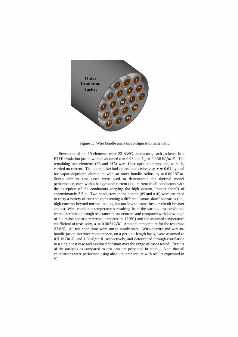
Figure 1: Wire bundle analysis configuration schematic.

Seventeen of the 19 elements were 22 AWG conductors, each jacketed in a

PTFE insulation jacket with an assumed 𝜀 = 0.93 and 𝑘𝑤 = 0.238 𝑊/𝑚 𝐾. The

remaining two elements (#6 and #15) were fiber optic elements and, as such,

carried no current. The outer jacket had an assumed emissivity, 𝜀 = 0.04, typical

for vapor deposited aluminum with an outer bundle radius, 𝑟𝑏 = 0.00287 𝑚.

Seven ambient test cases were used to demonstrate the thermal model

performance, each with a background current (i.e., current in all conductors with

the exception of the conductors carrying the high current, “smart short”) of

approximately 2.5 𝐴. Two conductors in the bundle (#5 and #10) were assumed

to carry a variety of currents representing a different “smart short” scenarios (i.e.,

high currents beyond normal loading but too low to cause fuse or circuit breaker

action). Wire conductor temperatures resulting from the various test conditions

were determined through resistance measurements and computed with knowledge

of the resistance at a reference temperature (20℃) and the assumed temperature

coefficient of resistivity, 𝛼 = 0.00342/𝐾. Ambient temperature for the tests was

22.8℃. All test conditions were run to steady state. Wire-to-wire and wire-to-

bundle jacket interface conductance, on a per unit length basis, were assumed to

0.5 𝑊 𝑚 𝐾⁄ and 1.0 𝑊 𝑚 𝐾⁄ , respectively, and determined through correlation

to a single test case and assumed constant over the range of cases tested. Results

of the analysis as compared to test data are presented in table 1. Note that all

calculations were performed using absolute temperature with results expressed in

℃.

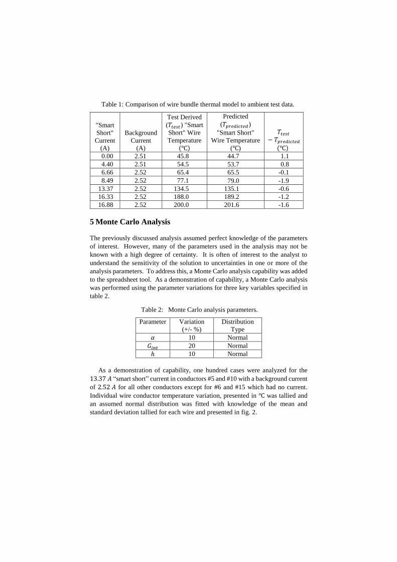
Table 1: Comparison of wire bundle thermal model to ambient test data.

"Smart

Short"

Current

(A)

Background

Current

(A)

Test Derived

(𝑇𝑡𝑒𝑠𝑡) "Smart

Short" Wire

Temperature

(℃)

Predicted

(𝑇𝑝𝑟𝑒𝑑𝑖𝑐𝑡𝑒𝑑)

"Smart Short"

Wire Temperature

(℃)

𝑇𝑡𝑒𝑠𝑡− 𝑇𝑝𝑟𝑒𝑑𝑖𝑐𝑡𝑒𝑑

(℃) 0.00 2.51 45.8 44.7 1.1

4.40 2.51 54.5 53.7 0.8

6.66 2.52 65.4 65.5 -0.1

8.49 2.52 77.1 79.0 -1.9

13.37 2.52 134.5 135.1 -0.6

16.33 2.52 188.0 189.2 -1.2

16.88 2.52 200.0 201.6 -1.6

5 Monte Carlo Analysis

The previously discussed analysis assumed perfect knowledge of the parameters

of interest. However, many of the parameters used in the analysis may not be

known with a high degree of certainty. It is often of interest to the analyst to

understand the sensitivity of the solution to uncertainties in one or more of the

analysis parameters. To address this, a Monte Carlo analysis capability was added

to the spreadsheet tool. As a demonstration of capability, a Monte Carlo analysis

was performed using the parameter variations for three key variables specified in

table 2.

Table 2: Monte Carlo analysis parameters.

Parameter Variation

(+/- %)

Distribution

Type

𝛼 10 Normal

𝐺𝑖𝑛𝑡 20 Normal

ℎ 10 Normal

As a demonstration of capability, one hundred cases were analyzed for the

13.37 𝐴 “smart short” current in conductors #5 and #10 with a background current

of 2.52 𝐴 for all other conductors except for #6 and #15 which had no current.

Individual wire conductor temperature variation, presented in ℃ was tallied and

an assumed normal distribution was fitted with knowledge of the mean and

standard deviation tallied for each wire and presented in fig. 2.

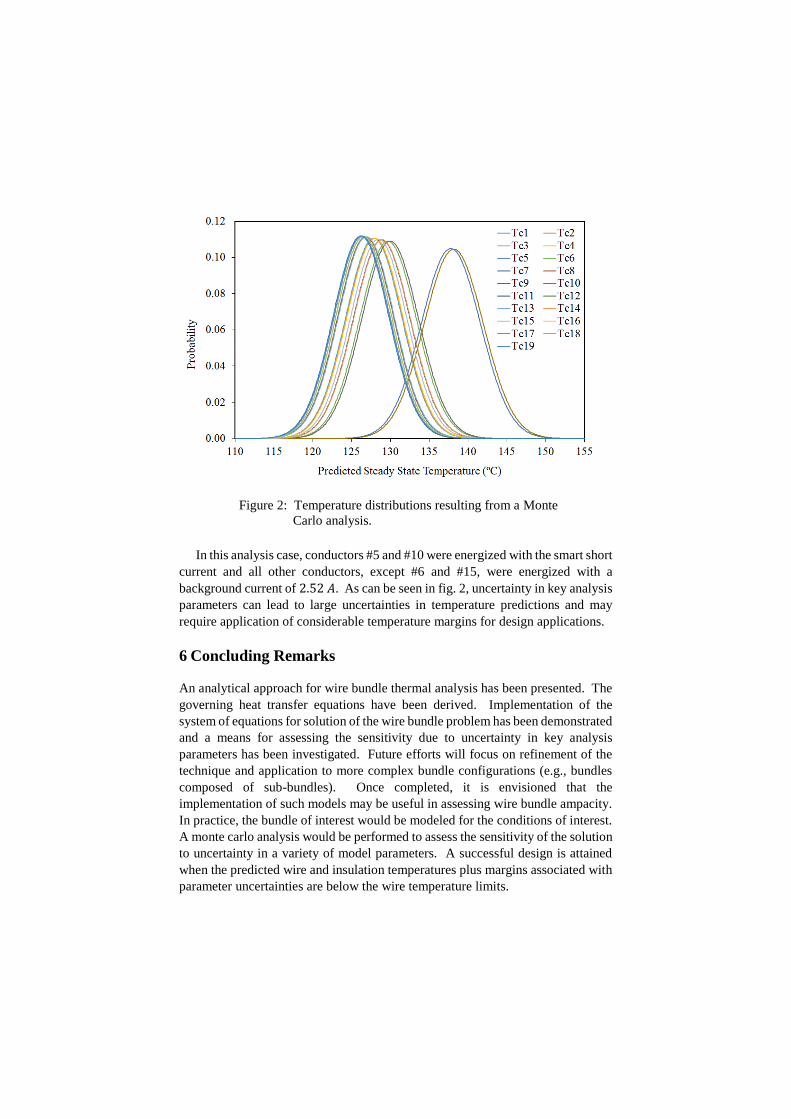
Figure 2: Temperature distributions resulting from a Monte

Carlo analysis.

In this analysis case, conductors #5 and #10 were energized with the smart short

current and all other conductors, except #6 and #15, were energized with a

background current of 2.52 𝐴. As can be seen in fig. 2, uncertainty in key analysis

parameters can lead to large uncertainties in temperature predictions and may

require application of considerable temperature margins for design applications.

6 Concluding Remarks

An analytical approach for wire bundle thermal analysis has been presented. The

governing heat transfer equations have been derived. Implementation of the

system of equations for solution of the wire bundle problem has been demonstrated

and a means for assessing the sensitivity due to uncertainty in key analysis

parameters has been investigated. Future efforts will focus on refinement of the

technique and application to more complex bundle configurations (e.g., bundles

composed of sub-bundles). Once completed, it is envisioned that the

implementation of such models may be useful in assessing wire bundle ampacity.

In practice, the bundle of interest would be modeled for the conditions of interest.

A monte carlo analysis would be performed to assess the sensitivity of the solution

to uncertainty in a variety of model parameters. A successful design is attained

when the predicted wire and insulation temperatures plus margins associated with

parameter uncertainties are below the wire temperature limits.

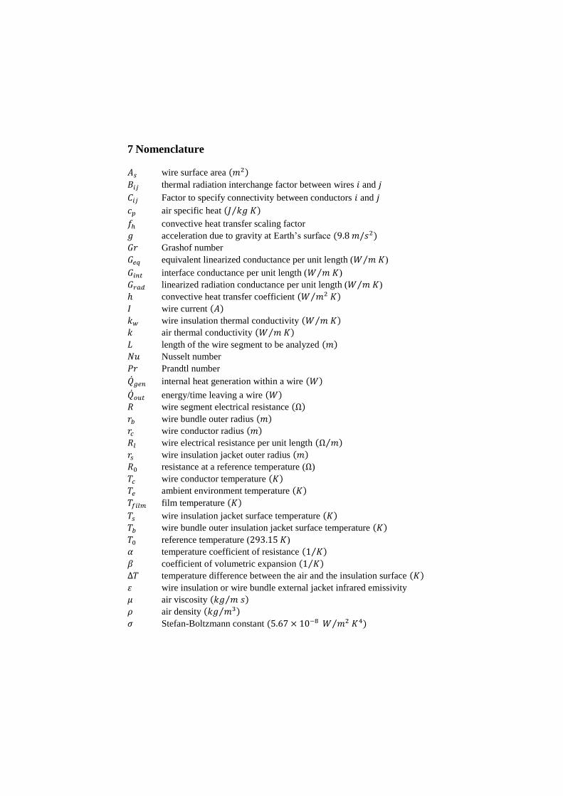
7 Nomenclature

𝐴𝑠 wire surface area (𝑚2)

𝐵𝑖𝑗 thermal radiation interchange factor between wires 𝑖 and 𝑗

𝐶𝑖𝑗 Factor to specify connectivity between conductors 𝑖 and 𝑗

𝑐𝑝 air specific heat (𝐽 𝑘𝑔 𝐾⁄ )

𝑓ℎ convective heat transfer scaling factor

𝑔 acceleration due to gravity at Earth’s surface (9.8 𝑚/𝑠2)

𝐺𝑟 Grashof number

𝐺𝑒𝑞 equivalent linearized conductance per unit length (𝑊 𝑚 𝐾⁄ )

𝐺𝑖𝑛𝑡 interface conductance per unit length (𝑊 𝑚 𝐾⁄ )

𝐺𝑟𝑎𝑑 linearized radiation conductance per unit length (𝑊 𝑚 𝐾⁄ )

ℎ convective heat transfer coefficient (𝑊 𝑚2 𝐾⁄ )

𝐼 wire current (𝐴)

𝑘𝑤 wire insulation thermal conductivity (𝑊 𝑚 𝐾⁄ )

𝑘 air thermal conductivity (𝑊 𝑚 𝐾⁄ )

𝐿 length of the wire segment to be analyzed (𝑚)

𝑁𝑢 Nusselt number

𝑃𝑟 Prandtl number

�̇�𝑔𝑒𝑛 internal heat generation within a wire (𝑊)

�̇�𝑜𝑢𝑡 energy/time leaving a wire (𝑊)

𝑅 wire segment electrical resistance (Ω)

𝑟𝑏 wire bundle outer radius (𝑚)

𝑟𝑐 wire conductor radius (𝑚)

𝑅𝑙 wire electrical resistance per unit length (Ω 𝑚⁄ )

𝑟𝑠 wire insulation jacket outer radius (𝑚)

𝑅0 resistance at a reference temperature (Ω)

𝑇𝑐 wire conductor temperature (𝐾)

𝑇𝑒 ambient environment temperature (𝐾)

𝑇𝑓𝑖𝑙𝑚 film temperature (𝐾)

𝑇𝑠 wire insulation jacket surface temperature (𝐾)

𝑇𝑏 wire bundle outer insulation jacket surface temperature (𝐾)

𝑇0 reference temperature (293.15 𝐾)

𝛼 temperature coefficient of resistance (1 𝐾⁄ )

𝛽 coefficient of volumetric expansion (1 𝐾⁄ )

Δ𝑇 temperature difference between the air and the insulation surface (𝐾)

𝜀 wire insulation or wire bundle external jacket infrared emissivity

𝜇 air viscosity (𝑘𝑔 𝑚 𝑠⁄ )

𝜌 air density (𝑘𝑔 𝑚3⁄ )

𝜎 Stefan-Boltzmann constant (5.67 × 10−8 𝑊 𝑚2 𝐾4⁄ )

8 Acknowledgements

The work described in this paper was performed with the sponsorship of the NASA

Engineering and Safety Center under the technical leadership of Dr. Robert Kichak

of AS and D, Inc. The authors acknowledge the test support provided by Mr. Thad

Johnson, Mr. Lawrence Ludwig, Mrs. Tamara Dodge, Mr. Dan Ciarlariello, and

Mr. Lawrence Batterson of the NASA – Kennedy Space Center.

9 References

[1] Cornelius, R.S., A History of the Development of New Current Ratings for

Aerospace Wire, RayChem Report, circa 1978.

[2] Wire Size Determination for Aerospace Applications, Report No. 88-220,

Eagle Engineering/LMESCO under Contract to NASA (NAS-17900),

December 1, 1988.

[3] Wire/Cable Selection, Report No. 2ITA017, McDonnell Douglas Space

Systems Company, May 10, 1990.

[4] van Benthem, R.C., de Grave, W., Doctor, F., Taylor, S.,Nuyten, K., & Dit

Routier, P.A.J., Thermal Analysis of Wiring Bundles for Weight Reduction

and Improved Safety, AIAA 2011-5111, National Aerospace Laboratory

(NLR), Netherlands, International Conference on Environmental Systems,

July 2011.

[5] A. Ilgevičius, H. D. Liess, Thermal Analysis of Electrical Wires by Finite

Volume Method, ISSN 1392 – 1215 Elektronika ir Elektrotechnika. 2003.

Nr. 4(46).

[6] J. P. Holman, Heat Transfer, 5th Edition, McGraw-Hill Book Company, New

York, pp. 274-277, 1981.