Embed Size (px)
Citation preview
Heuristic search
Weighted A∗
Kustaa Kangas
October 17, 2013
K. Kangas () Heuristic search Weighted A∗ October 17, 2013 1 / 47
Weighted A∗
Weighted A∗ search – unifying view and application
Rudiger Ebendt, Rolf Drechsler, 2009
Weighted A∗
Weight the heuristic to quickly direct the search.
Save time, get bounded suboptimality in exchange.
Outline
1 Three approaches: WA∗, DWA∗, A∗ε2 Unifying view
3 Monotone heuristic
4 Approximate BDD minimization
5 Experiments
K. Kangas () Heuristic search Weighted A∗ October 17, 2013 2 / 47
Standard A∗
Standard A∗
f (q) = g(q) + h(q)
Finds an optimal path if h is admissible, i.e. h(q) ≤ h∗(q).
K. Kangas () Heuristic search Weighted A∗ October 17, 2013 3 / 47
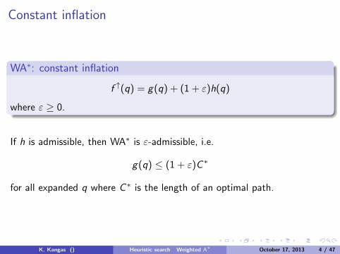
Constant inflation
WA∗: constant inflation
f ↑(q) = g(q) + (1 + ε)h(q)
where ε ≥ 0.
If h is admissible, then WA∗ is ε-admissible, i.e.
g(q) ≤ (1 + ε)C ∗
for all expanded q where C ∗ is the length of an optimal path.
K. Kangas () Heuristic search Weighted A∗ October 17, 2013 4 / 47
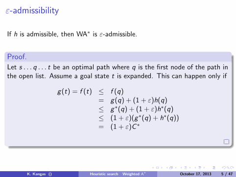
ε-admissibility
If h is admissible, then WA∗ is ε-admissible.
Proof.
Let s . . . q . . . t be an optimal path where q is the first node of the path inthe open list. Assume a goal state t is expanded. This can happen only if
g(t) = f (t) ≤ f (q)= g(q) + (1 + ε)h(q)≤ g∗(q) + (1 + ε)h∗(q)≤ (1 + ε)(g∗(q) + h∗(q))= (1 + ε)C ∗
K. Kangas () Heuristic search Weighted A∗ October 17, 2013 5 / 47
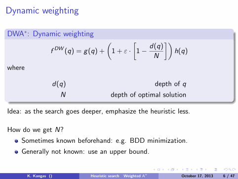
Dynamic weighting
DWA∗: Dynamic weighting
f DW (q) = g(q) +
(1 + ε ·
[1− d(q)
N
])h(q)
where
d(q) depth of q
N depth of optimal solution
Idea: as the search goes deeper, emphasize the heuristic less.
How do we get N?
Sometimes known beforehand: e.g. BDD minimization.
Generally not known: use an upper bound.
K. Kangas () Heuristic search Weighted A∗ October 17, 2013 6 / 47
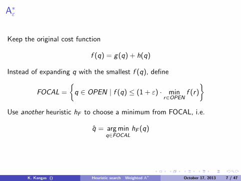
A∗ε
Keep the original cost function
f (q) = g(q) + h(q)
Instead of expanding q with the smallest f (q), define
FOCAL =
{q ∈ OPEN | f (q) ≤ (1 + ε) · min
r∈OPENf (r)
}Use another heuristic hF to choose a minimum from FOCAL, i.e.
q = arg minq∈FOCAL
hF (q)
K. Kangas () Heuristic search Weighted A∗ October 17, 2013 7 / 47
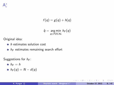
A∗ε
f (q) = g(q) + h(q)
q = arg minq∈FOCAL
hF (q)
Original idea:
h estimates solution cost
hF estimates remaining search effort
Suggestions for hF :
hF = h
hF (q) = N − d(q)
K. Kangas () Heuristic search Weighted A∗ October 17, 2013 8 / 47
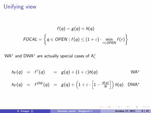
Unifying view
f (q) = g(q) + h(q)
FOCAL =
{q ∈ OPEN | f (q) ≤ (1 + ε) · min
r∈OPENf (r)
}
WA∗ and DWA∗ are actually special cases of A∗ε
hF (q) = f ↑(q) = g(q) + (1 + ε)h(q) WA∗
hF (q) = f DW (q) = g(q) +(
1 + ε ·[1− d(q)
N
])h(q) DWA∗
K. Kangas () Heuristic search Weighted A∗ October 17, 2013 9 / 47
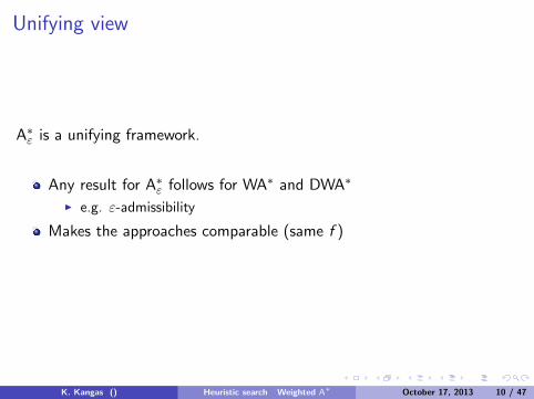
Unifying view
A∗ε is a unifying framework.
Any result for A∗ε follows for WA∗ and DWA∗
I e.g. ε-admissibility
Makes the approaches comparable (same f )
K. Kangas () Heuristic search Weighted A∗ October 17, 2013 10 / 47
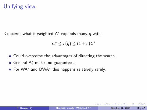
Unifying view
Concern: what if weighted A∗ expands many q with
C ∗ ≤ f (q) ≤ (1 + ε)C ∗
Could overcome the advantages of directing the search.
General A∗ε makes no guarantees.
For WA∗ and DWA∗ this happens relatively rarely.
K. Kangas () Heuristic search Weighted A∗ October 17, 2013 11 / 47
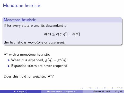
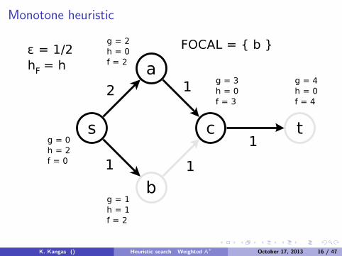
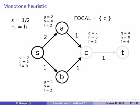
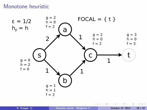
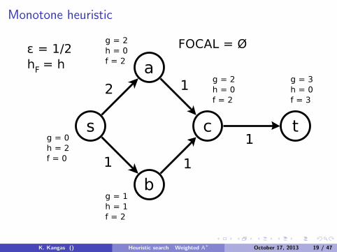
Monotone heuristic
Monotone heuristic
If for every state q and its descendant q′
h(q) ≤ c(q, q′) + h(q′)
the heuristic is monotone or consistent.
A∗ with a monotone heuristic
When q is expanded, g(q) = g∗(q)
Expanded states are never reopened
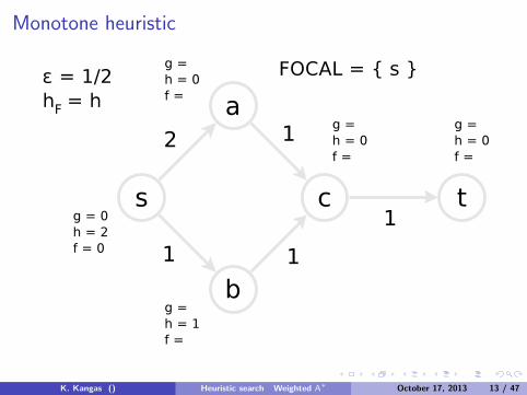
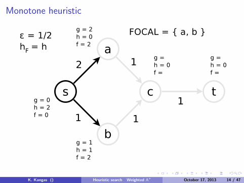
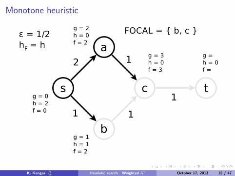
Does this hold for weighted A∗?
K. Kangas () Heuristic search Weighted A∗ October 17, 2013 12 / 47
Monotone heuristic
K. Kangas () Heuristic search Weighted A∗ October 17, 2013 13 / 47
Monotone heuristic
K. Kangas () Heuristic search Weighted A∗ October 17, 2013 14 / 47
Monotone heuristic
K. Kangas () Heuristic search Weighted A∗ October 17, 2013 15 / 47
Monotone heuristic
K. Kangas () Heuristic search Weighted A∗ October 17, 2013 16 / 47
Monotone heuristic
K. Kangas () Heuristic search Weighted A∗ October 17, 2013 17 / 47
Monotone heuristic
K. Kangas () Heuristic search Weighted A∗ October 17, 2013 18 / 47
Monotone heuristic
K. Kangas () Heuristic search Weighted A∗ October 17, 2013 19 / 47
Monotone heuristic
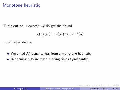
Turns out no. However, we do get the bound
g(q) ≤ (1 + ε)g∗(q) + ε · h(q)
for all expanded q.
Weighted A∗ benefits less from a monotone heuristic.
Reopening may increase running times significantly.
K. Kangas () Heuristic search Weighted A∗ October 17, 2013 20 / 47
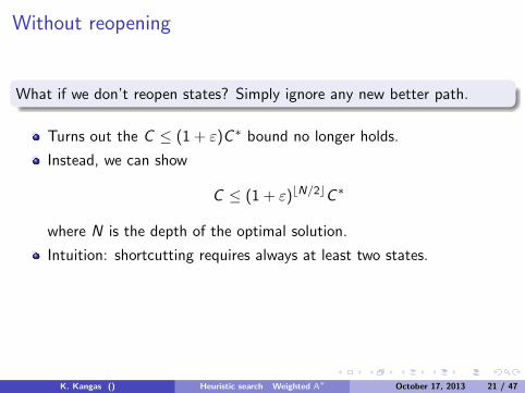
Without reopening
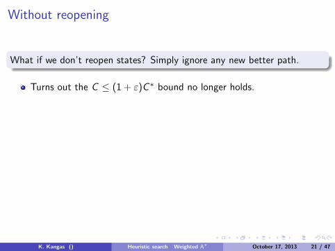
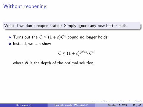
What if we don’t reopen states? Simply ignore any new better path.
Turns out the C ≤ (1 + ε)C ∗ bound no longer holds.
Instead, we can show
C ≤ (1 + ε)bN/2cC ∗
where N is the depth of the optimal solution.
Intuition: shortcutting requires always at least two states.
Each shortcut accumulates the error by a factor of (1 + ε).
WA∗ and DWA∗ are still ε-admissible without reopening.
K. Kangas () Heuristic search Weighted A∗ October 17, 2013 21 / 47
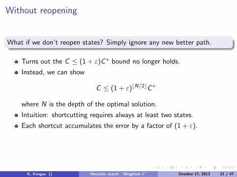
Without reopening
What if we don’t reopen states? Simply ignore any new better path.
Turns out the C ≤ (1 + ε)C ∗ bound no longer holds.
Instead, we can show
C ≤ (1 + ε)bN/2cC ∗
where N is the depth of the optimal solution.
Intuition: shortcutting requires always at least two states.
Each shortcut accumulates the error by a factor of (1 + ε).
WA∗ and DWA∗ are still ε-admissible without reopening.
K. Kangas () Heuristic search Weighted A∗ October 17, 2013 21 / 47
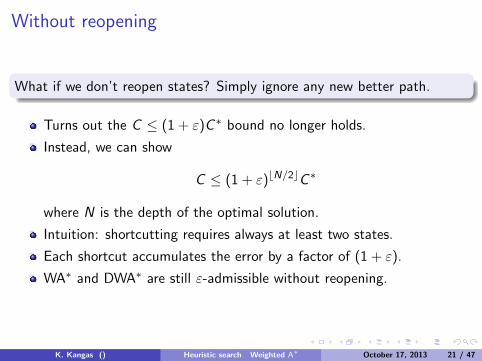
Without reopening
What if we don’t reopen states? Simply ignore any new better path.
Turns out the C ≤ (1 + ε)C ∗ bound no longer holds.
Instead, we can show
C ≤ (1 + ε)bN/2cC ∗
where N is the depth of the optimal solution.
Intuition: shortcutting requires always at least two states.
Each shortcut accumulates the error by a factor of (1 + ε).
WA∗ and DWA∗ are still ε-admissible without reopening.
K. Kangas () Heuristic search Weighted A∗ October 17, 2013 21 / 47
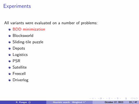
Experiments
All variants were evaluated on a number of problems:
BDD minimization
Blocksworld
Sliding-tile puzzle
Depots
Logistics
PSR
Satellite
Freecell
Driverlog
K. Kangas () Heuristic search Weighted A∗ October 17, 2013 22 / 47
Experiments
All variants were evaluated on a number of problems:
BDD minimization
Blocksworld
Sliding-tile puzzle
Depots
Logistics
PSR
Satellite
Freecell
Driverlog
K. Kangas () Heuristic search Weighted A∗ October 17, 2013 23 / 47
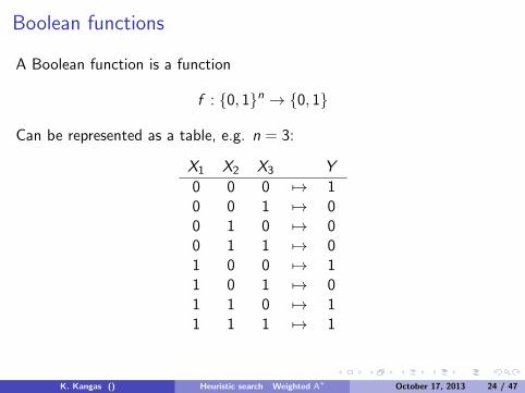
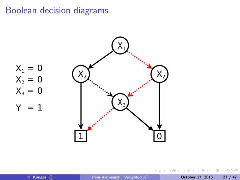
Boolean functions
A Boolean function is a function
f : {0, 1}n → {0, 1}
Can be represented as a table, e.g. n = 3:
X1 X2 X3 Y
0 0 0 7→ 10 0 1 7→ 00 1 0 7→ 00 1 1 7→ 01 0 0 7→ 11 0 1 7→ 01 1 0 7→ 11 1 1 7→ 1
K. Kangas () Heuristic search Weighted A∗ October 17, 2013 24 / 47
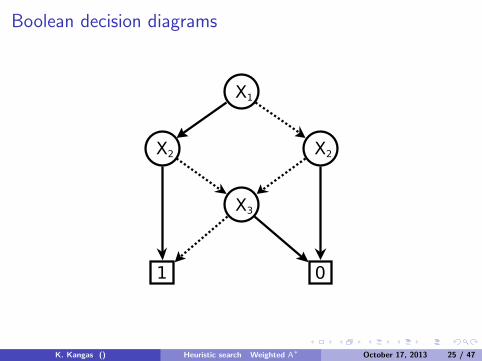
Boolean decision diagrams
K. Kangas () Heuristic search Weighted A∗ October 17, 2013 25 / 47
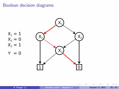
Boolean decision diagrams
K. Kangas () Heuristic search Weighted A∗ October 17, 2013 26 / 47
Boolean decision diagrams
K. Kangas () Heuristic search Weighted A∗ October 17, 2013 27 / 47
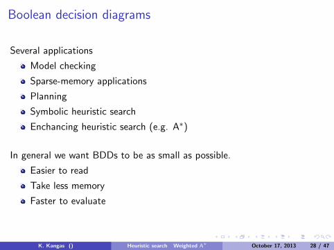
Boolean decision diagrams
Several applications
Model checking
Sparse-memory applications
Planning
Symbolic heuristic search
Enchancing heuristic search (e.g. A∗)
In general we want BDDs to be as small as possible.
Easier to read
Take less memory
Faster to evaluate
K. Kangas () Heuristic search Weighted A∗ October 17, 2013 28 / 47
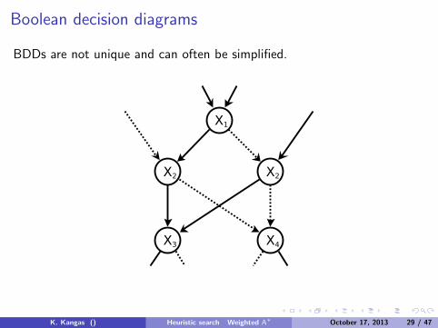
Boolean decision diagrams
BDDs are not unique and can often be simplified.
K. Kangas () Heuristic search Weighted A∗ October 17, 2013 29 / 47

Boolean decision diagrams
BDDs are not unique and can often be simplified.
K. Kangas () Heuristic search Weighted A∗ October 17, 2013 30 / 47
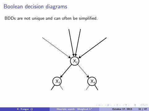
Boolean decision diagrams
BDDs are not unique and can often be simplified.
K. Kangas () Heuristic search Weighted A∗ October 17, 2013 31 / 47
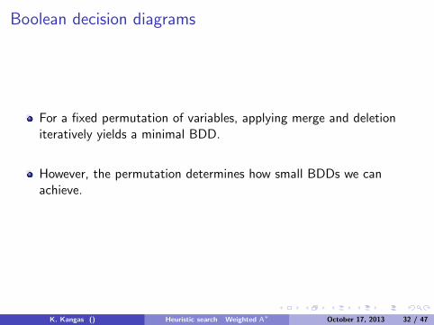
Boolean decision diagrams
For a fixed permutation of variables, applying merge and deletioniteratively yields a minimal BDD.
However, the permutation determines how small BDDs we canachieve.
K. Kangas () Heuristic search Weighted A∗ October 17, 2013 32 / 47
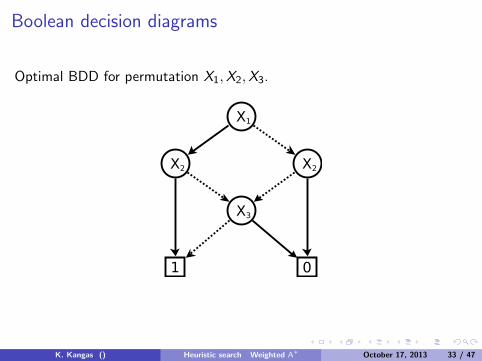
Boolean decision diagrams
Optimal BDD for permutation X1,X2,X3.
K. Kangas () Heuristic search Weighted A∗ October 17, 2013 33 / 47
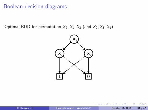
Boolean decision diagrams
Optimal BDD for permutation X2,X1,X3 (and X2,X3,X1)
K. Kangas () Heuristic search Weighted A∗ October 17, 2013 34 / 47
Boolean decision diagrams
BDD minimization problem: find an ordering of variables that yields aminimal BDD (least nodes)
NP-hard (decision version is NP-complete)
Can be solved exactly in O(3nn).
Can often be solved fast with heuristic search.
K. Kangas () Heuristic search Weighted A∗ October 17, 2013 35 / 47
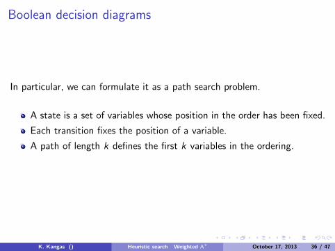
Boolean decision diagrams
In particular, we can formulate it as a path search problem.
A state is a set of variables whose position in the order has been fixed.
Each transition fixes the position of a variable.
A path of length k defines the first k variables in the ordering.
K. Kangas () Heuristic search Weighted A∗ October 17, 2013 36 / 47
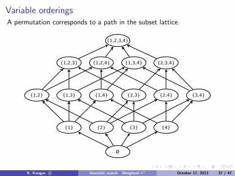
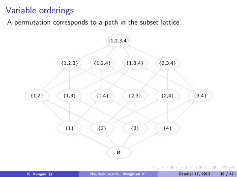
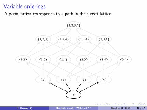
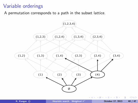
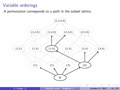
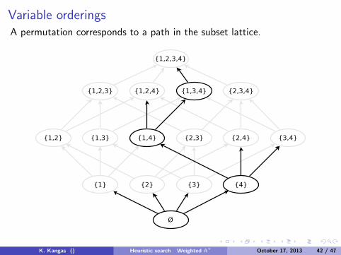
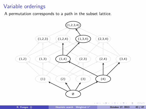
Variable orderingsA permutation corresponds to a path in the subset lattice.
K. Kangas () Heuristic search Weighted A∗ October 17, 2013 37 / 47
Variable orderingsA permutation corresponds to a path in the subset lattice.
K. Kangas () Heuristic search Weighted A∗ October 17, 2013 38 / 47
Variable orderingsA permutation corresponds to a path in the subset lattice.
K. Kangas () Heuristic search Weighted A∗ October 17, 2013 39 / 47
Variable orderingsA permutation corresponds to a path in the subset lattice.
K. Kangas () Heuristic search Weighted A∗ October 17, 2013 40 / 47
Variable orderingsA permutation corresponds to a path in the subset lattice.
K. Kangas () Heuristic search Weighted A∗ October 17, 2013 41 / 47
Variable orderingsA permutation corresponds to a path in the subset lattice.
K. Kangas () Heuristic search Weighted A∗ October 17, 2013 42 / 47
Variable orderingsA permutation corresponds to a path in the subset lattice.
K. Kangas () Heuristic search Weighted A∗ October 17, 2013 43 / 47
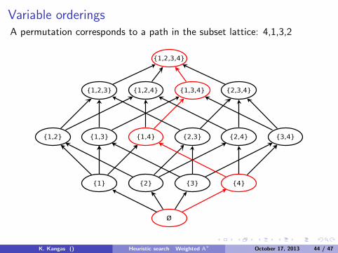
Variable orderingsA permutation corresponds to a path in the subset lattice: 4,1,3,2
K. Kangas () Heuristic search Weighted A∗ October 17, 2013 44 / 47
Variable orderings
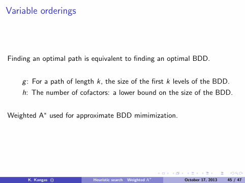
Finding an optimal path is equivalent to finding an optimal BDD.
g : For a path of length k, the size of the first k levels of the BDD.
h: The number of cofactors: a lower bound on the size of the BDD.
Weighted A∗ used for approximate BDD mimimization.
K. Kangas () Heuristic search Weighted A∗ October 17, 2013 45 / 47
Experiments
Experimental results.
K. Kangas () Heuristic search Weighted A∗ October 17, 2013 46 / 47
Questions?
K. Kangas () Heuristic search Weighted A∗ October 17, 2013 47 / 47