HEURISTIC SEARCH WITH LIMITED MEMORY

BY

Matthew Hatem

Bachelor’s in Computer Science, Plymouth State College, 1999

Master’s in Computer Science, University of New Hampshire, 2010

DISSERTATION

Submitted to the University of New Hampshire

in Partial Fulfillment of

the Requirements for the Degree of

Doctor of Philosophy

in

Computer Science

May, 2014

ALL RIGHTS RESERVED

c©2014

Matthew Hatem

This dissertation has been examined and approved.

Dissertation director, Wheeler Ruml,Associate Professor of Computer ScienceUniversity of New Hampshire

Radim Bartos,Associate Professor, Chair of Computer ScienceUniversity of New Hampshire

R. Daniel Bergeron,Professor of Computer ScienceUniversity of New Hampshire

Philip J. Hatcher,Professor of Computer ScienceUniversity of New Hampshire

Richard Korf,Professor of Computer ScienceUniversity of California, Los Angeles

Date

DEDICATION

To Noah, my greatest achievement.

iv

ACKNOWLEDGMENTS

If I have seen further it is by standing on the shoulders of giants.

– Isaac Newton

My family has provided the support necessary to keep me working at all hours of the

day and night. My wife Kate, who has the hardest job in the world, has been especially

patient and supportive even when she probably shouldn’t have. My parents, Alison and

Clifford, have made life really easy for me and for that I am eternally grateful.

Working with my advisor, Wheeler Ruml, has been the most rewarding aspect of this

entire endeavor. I would have given up years ago were it not for his passion, persistence

and just the right amount of encouragement (actually, I tried to quit twice and he did not

let me). He has taught me how to be a better writer, programmer, researcher, speaker and

student. Wheeler exhibits a level of excellence that I have not seen in anyone before. He is

the best at what he does and I am fortunate to have worked with him.

Many fellow students have helped me along the way, especially Ethan Burns. Ethan

set the bar incredibly high and showed that it was possible to satisfy Wheeler. All of the

plots in this dissertation were generated by a plotting program that Ethan and Jordan

Thayer developed over the course of a summer. Some of the code I wrote to conduct my

experiments borrowed heavily from Ethan’s. I would have been lost without it.

Scott Kiesel helped me with the majority of Chapter 6. I’m grateful for his contribution

and his patience as we worked through the most complex proof I have ever been involved

with.

Finally, I would like to thank all the members of my committee, especially Richard Korf,

who provided me with some of the most insightful feedback and whose work has inspired

nearly every chapter of this dissertation.

This work has been funded primarily by NSF, DARPA, IBM and myself.

v

TABLE OF CONTENTS

DEDICATION . . . . . . . . . . . . . . . . . . . . . . . . . . . . . . . . . . . . . iv

ACKNOWLEDGMENTS . . . . . . . . . . . . . . . . . . . . . . . . . . . . . . . v

LIST OF TABLES . . . . . . . . . . . . . . . . . . . . . . . . . . . . . . . . . . . ix

LIST OF FIGURES . . . . . . . . . . . . . . . . . . . . . . . . . . . . . . . . . . xii

ABSTRACT . . . . . . . . . . . . . . . . . . . . . . . . . . . . . . . . . . . . . . xiii

Chapter 1 INTRODUCTION AND OVERVIEW 1

1.1 Heuristic Search . . . . . . . . . . . . . . . . . . . . . . . . . . . . . . . . . 2

1.2 Heuristic Search with Limited Memory . . . . . . . . . . . . . . . . . . . . . 6

1.3 Real-World Problems . . . . . . . . . . . . . . . . . . . . . . . . . . . . . . . 9

1.4 Dissertation Outline . . . . . . . . . . . . . . . . . . . . . . . . . . . . . . . 12

Chapter 2 EXTERNAL MEMORY SEARCH 15

2.1 Introduction . . . . . . . . . . . . . . . . . . . . . . . . . . . . . . . . . . . . 15

2.2 Delayed Duplicate Detection . . . . . . . . . . . . . . . . . . . . . . . . . . 16

2.3 Parallel External A* . . . . . . . . . . . . . . . . . . . . . . . . . . . . . . . 18

2.4 Empirical Results . . . . . . . . . . . . . . . . . . . . . . . . . . . . . . . . . 21

2.5 Discussion . . . . . . . . . . . . . . . . . . . . . . . . . . . . . . . . . . . . . 23

2.6 Conclusion . . . . . . . . . . . . . . . . . . . . . . . . . . . . . . . . . . . . 24

Chapter 3 EXTERNAL SEARCH: NON-UNIFORM EDGE COSTS 25

3.1 Introduction . . . . . . . . . . . . . . . . . . . . . . . . . . . . . . . . . . . . 25

3.2 Previous Work . . . . . . . . . . . . . . . . . . . . . . . . . . . . . . . . . . 26

3.3 Parallel External Dynamic A* Layering . . . . . . . . . . . . . . . . . . . . 29

3.4 Conclusion . . . . . . . . . . . . . . . . . . . . . . . . . . . . . . . . . . . . 36

vi

Chapter 4 EXTERNAL SEARCH: LARGE BRANCHING FACTORS 37

4.1 Introduction . . . . . . . . . . . . . . . . . . . . . . . . . . . . . . . . . . . . 37

4.2 Multiple Sequence Alignment . . . . . . . . . . . . . . . . . . . . . . . . . . 39

4.3 Previous Work . . . . . . . . . . . . . . . . . . . . . . . . . . . . . . . . . . 43

4.4 Parallel External Memory PEA* . . . . . . . . . . . . . . . . . . . . . . . . 46

4.5 Empirical Evaluation . . . . . . . . . . . . . . . . . . . . . . . . . . . . . . . 48

4.6 Discussion . . . . . . . . . . . . . . . . . . . . . . . . . . . . . . . . . . . . . 51

4.7 Other Related Work . . . . . . . . . . . . . . . . . . . . . . . . . . . . . . . 52

4.8 Conclusion . . . . . . . . . . . . . . . . . . . . . . . . . . . . . . . . . . . . 54

Chapter 5 BOUNDED SUBOPTIMAL SEARCH 55

5.1 Introduction . . . . . . . . . . . . . . . . . . . . . . . . . . . . . . . . . . . . 55

5.2 Previous Work . . . . . . . . . . . . . . . . . . . . . . . . . . . . . . . . . . 57

5.3 Simplified Bounded Suboptimal Search . . . . . . . . . . . . . . . . . . . . . 60

5.4 Empirical Evaluation . . . . . . . . . . . . . . . . . . . . . . . . . . . . . . . 63

5.5 Discussion . . . . . . . . . . . . . . . . . . . . . . . . . . . . . . . . . . . . . 69

5.6 Conclusion . . . . . . . . . . . . . . . . . . . . . . . . . . . . . . . . . . . . 70

Chapter 6 HEURISTIC SEARCH IN LINEAR SPACE 72

6.1 Introduction . . . . . . . . . . . . . . . . . . . . . . . . . . . . . . . . . . . . 72

6.2 Previous Work . . . . . . . . . . . . . . . . . . . . . . . . . . . . . . . . . . 73

6.3 RBFS with Controlled Re-expansion . . . . . . . . . . . . . . . . . . . . . . 76

6.4 Empirical Evaluation . . . . . . . . . . . . . . . . . . . . . . . . . . . . . . . 82

6.5 Discussion . . . . . . . . . . . . . . . . . . . . . . . . . . . . . . . . . . . . . 85

6.6 Conclusion . . . . . . . . . . . . . . . . . . . . . . . . . . . . . . . . . . . . 86

Chapter 7 BOUNDED SUBOPTIMAL SEARCH IN LINEAR SPACE 87

7.1 Introduction . . . . . . . . . . . . . . . . . . . . . . . . . . . . . . . . . . . . 87

7.2 Previous Work . . . . . . . . . . . . . . . . . . . . . . . . . . . . . . . . . . 88

7.3 Using Solution Length Estimates . . . . . . . . . . . . . . . . . . . . . . . . 89

vii

7.4 Iterative Deepening A∗

ǫ . . . . . . . . . . . . . . . . . . . . . . . . . . . . . . 92

7.5 Recursive Best-First A∗

ǫ and EES . . . . . . . . . . . . . . . . . . . . . . . . 95

7.6 Empirical Evaluation . . . . . . . . . . . . . . . . . . . . . . . . . . . . . . . 96

7.7 Conclusion . . . . . . . . . . . . . . . . . . . . . . . . . . . . . . . . . . . . 100

Chapter 8 CONCLUSION 101

Bibliography 105

viii

LIST OF TABLES

2-1 Performance summary on the unit 15-puzzle. Times reported in seconds

for solving all instances. . . . . . . . . . . . . . . . . . . . . . . . . . . . 22

3-1 Performance summary for 15-puzzle with square root costs. Times re-

ported in seconds for solving all instances. . . . . . . . . . . . . . . . . . 33

3-2 Performance summary for Dockyard Robots. Times reported in seconds

for solving all instances. . . . . . . . . . . . . . . . . . . . . . . . . . . . 34

4-1 Results for the 75 easiest instances. Times reported in seconds for solving

all 75 instances. . . . . . . . . . . . . . . . . . . . . . . . . . . . . . . . . 49

4-2 Results for the 7 hardest instances of the BAliBASE Reference Set 1.

Expanded and generated counts reported in millions and times reported

in days:hours:minutes:seconds. . . . . . . . . . . . . . . . . . . . . . . . . 50

5-1 McCabe’s Cyclomatic Complexity (CC) and lines of code (LoC) metrics

for our implementations. . . . . . . . . . . . . . . . . . . . . . . . . . . . 68

ix

LIST OF FIGURES

1-1 A visual comparison of breadth-first search and A* search. Breadth-first

search explores a much larger portion of the search space while A* search

explores only the portion that appears most promising. . . . . . . . . . . 4

1-2 A* orders the search using the evaluation function f(n) = g(n) + h(n).

Nodes with lower f are estimated to be on a cheaper path to the goal and

thus, more promising to explore. . . . . . . . . . . . . . . . . . . . . . . 5

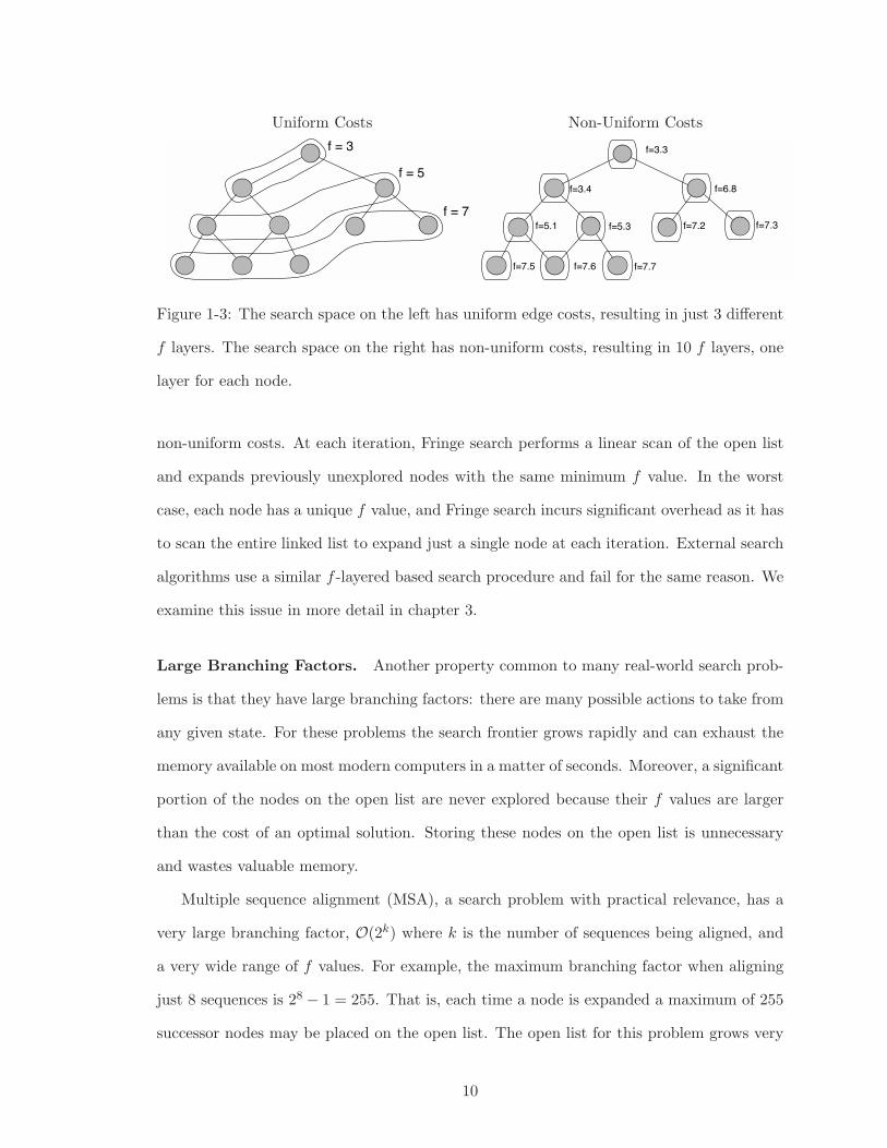
1-3 The search space on the left has uniform edge costs, resulting in just 3

different f layers. The search space on the right has non-uniform costs,

resulting in 10 f layers, one layer for each node. . . . . . . . . . . . . . . 10

1-4 A search space where distance-to-go estimates provide search guidance.

Best-first search would normally expand the node estimated to have least

cost f = 3. However, this would require more search effort than expanding

the node estimated to be closer to the goal d = 1. . . . . . . . . . . . . . 12

2-1 Pseudocode for A*-DDD. . . . . . . . . . . . . . . . . . . . . . . . . . . 19

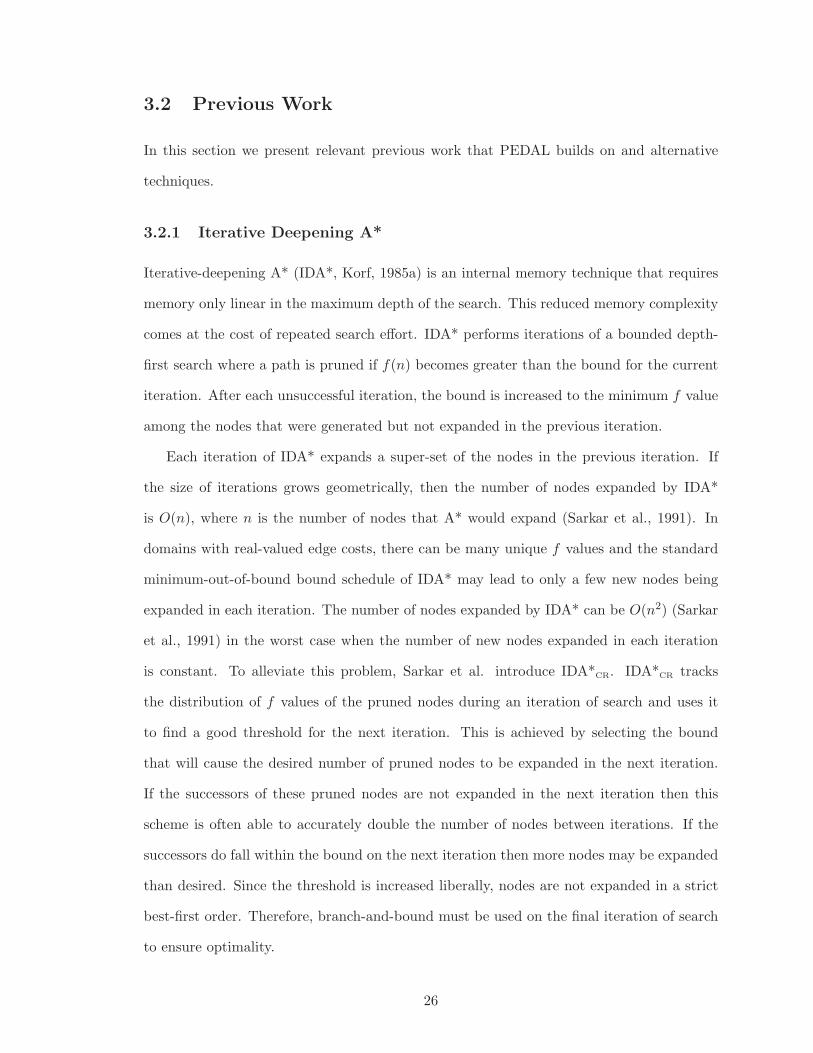
3-1 An example search tree showing the difference between a best-first search

with optimal tie-breaking and BFHS. The middle figure highlights the

nodes (labeled with their f values) expanded by a best-first search with

optimal tie breaking and the figure on the right highlights the nodes

expanded by BFHS. BFHS must expand all nodes that have an f equal

to the optimal solution cost, and is equivalent to best-first search with

worst-case tie-breaking. . . . . . . . . . . . . . . . . . . . . . . . . . . . 28

3-2 Pseudocode for PEDAL. . . . . . . . . . . . . . . . . . . . . . . . . . . . 29

x

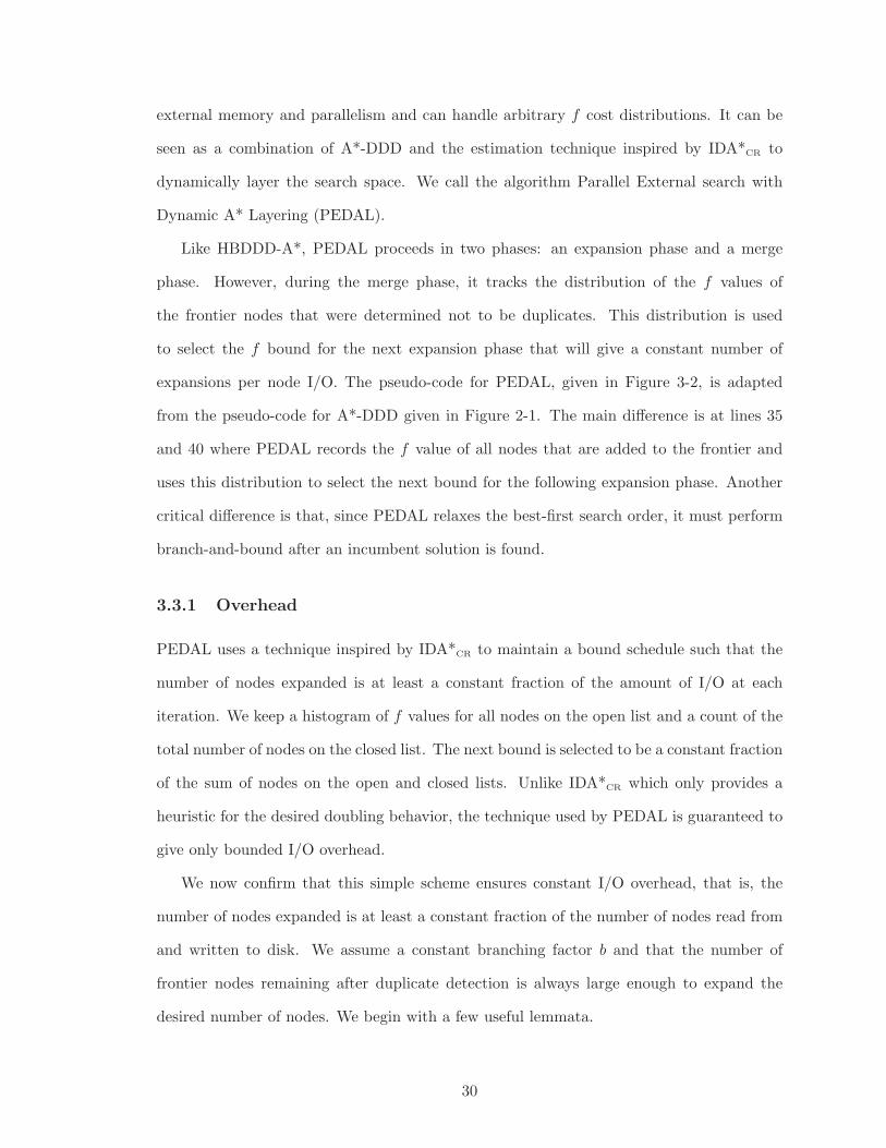
3-3 PEDAL keeps a histogram of f values on the open list and uses it to

update the threshold to allow for a constant fraction of the number of

nodes on open and closed to be expanded in each iteration. . . . . . . . 31

3-4 Comparison between PEDAL, IDA*CR, and BFHS-DDD. The axes show

Log10 CPU time. . . . . . . . . . . . . . . . . . . . . . . . . . . . . . . . 33

4-1 Optimal sequence alignment using a lattice and scoring matrix. . . . . . 39

4-2 Computing edge costs with affine gaps. The cost of edge E depends on

the incoming edge; one of h, d or v. If the incoming edge is v or d, then E

represents the start of a gap, and incurs a gap start penalty of 8. However,

if the incoming edge is h then E represents the continuation of a gap and

incurs no gap start penalty. . . . . . . . . . . . . . . . . . . . . . . . . . 41

4-3 Computing cost-to-go by solving the lattice in reverse. . . . . . . . . . . 43

4-4 Pseudocode for the PE2A* algorithm. . . . . . . . . . . . . . . . . . . . 47

5-1 Pseudo-code for node selection in EES. . . . . . . . . . . . . . . . . . . . 58

5-2 Pseudo-code for SEES. Ignoring the code in square brackets gives pseudo-

code for SA∗

ǫ . . . . . . . . . . . . . . . . . . . . . . . . . . . . . . . . . . 60

5-3 Comparison between SA∗

ǫ , SEES, EES and WA∗ on sliding tiles domains.

Plots show mean node expansions and mean CPU time in log10. . . . . . 64

5-4 Comparison between SA∗

ǫ , SEES, EES and WA∗ on pancakes and vacuum

world domains. Plots show mean node expansions and mean CPU time

in log10. . . . . . . . . . . . . . . . . . . . . . . . . . . . . . . . . . . . . 66

6-1 Pseudo-code for RBFS. . . . . . . . . . . . . . . . . . . . . . . . . . . . . 75

6-2 Pseudo-code for RBFSCR. . . . . . . . . . . . . . . . . . . . . . . . . . . 78

6-3 Mean log10 CPU time (top), nodes expanded (middle) and solution cost

(bottom) for the 15-Puzzle. . . . . . . . . . . . . . . . . . . . . . . . . . 83

6-4 Anytime Search Profiles for the 15-Puzzle. . . . . . . . . . . . . . . . . . 84

xi

7-1 Total CPU time (in log10) for A∗

ǫ and EES using estimates of total solution

length vs. estimates of distance-to-go. . . . . . . . . . . . . . . . . . . . 90

7-2 Pseudo-code for IDA∗

ǫ using l. . . . . . . . . . . . . . . . . . . . . . . . . 93

7-3 Pseudo-code for IDEES. . . . . . . . . . . . . . . . . . . . . . . . . . . . 94

7-4 Pseudo-code for RBA∗

ǫ (excluding the bracketed portions) and RBEES

(including the bracketed portions). . . . . . . . . . . . . . . . . . . . . . 96

7-5 Total CPU time and solution cost for the linear-space algorithms (in log10). 98

7-6 Total CPU time and solution cost for the linear-space algorithms (in log10). 99

xii

ABSTRACT

HEURISTIC SEARCH WITH LIMITED MEMORY

by

Matthew Hatem

University of New Hampshire, May, 2014

Heuristic search algorithms are commonly used for solving problems in artificial intel-

ligence. Unfortunately, the memory requirement of A*, the most widely used heuristic

search algorithm, is often proportional to its running time, making it impractical for large

problems. Several techniques exist for scaling heuristic search: external memory, bounded

suboptimal search, and linear-space algorithms. I address limitations in each. The thesis of

this dissertation is that in order to improve scalability, memory efficient heuristic search al-

gorithms benefit from the same techniques used in unbounded space search: best-first search

order, partial expansion, bounded node generation overhead, and distance-to-go estimates.

The four contributions of this dissertation make it easier to apply heuristic search to

challenging problems with practical relevance. First I address limitations in external mem-

ory search with a technique for bounding overhead on problems that have real-valued costs

and a another technique for reducing overhead on problems that have large branching fac-

tors. I demonstrate that these techniques achieve a new state-of-the-art on the problem

of multiple sequence alignment. Second, I examine recent work in bounded suboptimal

search and present a new technique for simplifying implementation and reducing run-time

overhead. The third contribution addresses limitations of linear-space search with a new

technique for provably bounding node regeneration overhead. Finally, I present four new

algorithms that advance the state of the art in linear space bounded suboptimal search.

These advances support the conclusion that search under memory limiations benefits from

techniques similar to those in unbounded space search.

xiii

CHAPTER 1

INTRODUCTION AND OVERVIEW

Many problems in computer science can be represented by a graph data structure, with paths

in the graph representing potential solutions. Finding an optimal solution to such a problem

requires finding a shortest or least-cost path between two nodes in the graph. Heuristic

search algorithms, used throughout the fields of artificial intelligence and robotics, find

solutions more efficiently than other techniques by exploring a much smaller portion of the

graph. Robot planning and path-finding are common applications of heuristic search. Other

problems, such as the parsing of natural language text and multiple sequence alignment,

can be formulated as a search problem and solved with heuristic search.

In order to find optimal solutions, popular heuristic search algorithms such as A* (Hart,

Nilsson, & Raphael, 1968), store every unique node they encounter in the graph. For large

problems, the memory required to store these nodes often exceeds the amount of memory

available on most modern computers. Several techniques exist for scaling heuristic search.

External memory search algorithms take advantage of cheap and plentiful secondary stor-

age, such as hard disks, to solve much larger problems than algorithms that only use main

memory. Linear-space search algorithms only require memory linear in the depth of the

search and bounded suboptimal search algorithms trade increased solution cost in a prin-

cipled way for significantly reduced solving time and memory. However, these techniques

often assume that problems exhibit certain properties that are not found in many real-world

problems, such as a uniform weight for all edges in the graph, limiting their application.

Moreover, they fail to take advantage of inadmissible heuristics and distance-to-go esti-

mates to solve problems more efficiently. The thesis of this dissertation is that in order

to improve scalability, memory efficient heuristic search algorithms benefit from the same

1

ideas behind techniques used in unbounded space search: best-first search order, partial

expansion, bounded node generation overhead, and distance-to-go estimates.

This dissertation makes four contributions that advance the state-of-the-art and make

it possible to apply heuristic search to challenging problems with practical relevance. First

we address limitations in external memory search with two new algorithms. The first

algorithm introduces a technique for bounding overhead on problems that have a wide

range of edge costs and the second algorithm introduces a technique for reducing overhead

on problems that have large branching factors. In an empirical evaluation we demonstrate

that these techniques achieve a new state-of-the-art on the problem of multiple sequence

alignment, a real-world problem that exhibits both a wide range of edge costs and large

branching factors. Next, we examine recent work in bounded suboptimal search and present

a method for dramatically simplifying implementation and reducing run-time overhead.

The third contribution addresses limitations of linear-space search by introducing a new

technique for provably bounding node regeneration overhead. Finally, I present four new

algorithms that advance the state of the art in linear space bounded suboptimal search.

These advances support the conclusion that search under memory limitations benefits from

techniques similar to those in unbounded space search.

1.1 Heuristic Search

In this section we review heuristic search and introduce much of the terminology used

throughout this dissertation.

A search problem is often formulated as a graph where a node in the graph corresponds

to a particular path to a problem state or state of the world, eg., the location and orientation

of an agent on a map. The edges in the graph represent the various actions that transition

the agent from one state to the other and each action has an associated cost represented

by the weight of the corresponding edge. The cost of a path between any two nodes in the

graph is the sum of the cost of all edges along the path.

The sliding-tiles puzzle is a simple problem with well-understood properties and is a

2

standard benchmark for evaluating search algorithms. The 15 puzzle is a type of sliding-

tiles puzzle that has 15 tiles arranged on a 4x4 grid. A tile has 16 possible locations,

with one location always being empty. Tiles adjacent to the empty location can slide from

one location to the other. The objective is to slide tiles until a goal configuration of the

puzzle is reached. We can model the 15 puzzle with a graph by representing each possible

configuration of the tiles as nodes in the graph. An edge connects two nodes if there is a

single action that transforms one configuration into the other. An action in this domain is

sliding a tile into the blank space. There are 16! possible ways to arrange 15 tiles on the

grid, but there are actually 16!/2 = 10, 461, 394, 944, 000 reachable configurations or states

of the 15 puzzle. This is because the physical constraints of the puzzle allow us to reach

exactly half of all possible configurations. The memory required to store just the reachable

states far exceeds the memory limit of most modern computers.

Depth-first search and breadth-first search are common examples of algorithms for find-

ing paths in a graph. However, they are uninformed, and they are often severely limited in

the size of the problems they can solve. Moreover, depth-first search is not guaranteed to

find an optimal solution (or any solution at all in some cases), and breadth-first search is

guaranteed to find an optimal solution only in special cases. Heuristic search, in contrast,

is an informed search that exploits knowledge about a problem, encoded in a heuristic,

to solve the problem more efficiently. Heuristic search algorithms can solve many difficult

problems that uninformed algorithms cannot.

A* or some variation of it, is one of the most widely used heuristic search algorithms

today. It can be viewed as an extension of Dijkstra’s algorithm (Dijkstra, 1959) that

exploits knowledge about a problem to reduce the number of computations necessary to

find a solution while still guaranteeing optimal solutions. The A* and Dijkstra’s algorithms

are classic examples of best-first graph-traversal algorithms. They are best-first because

they visit the best-looking nodes — the nodes that appear to be on a shortest path to

a goal — first until a solution is found. For many problems, it is critical to find optimal

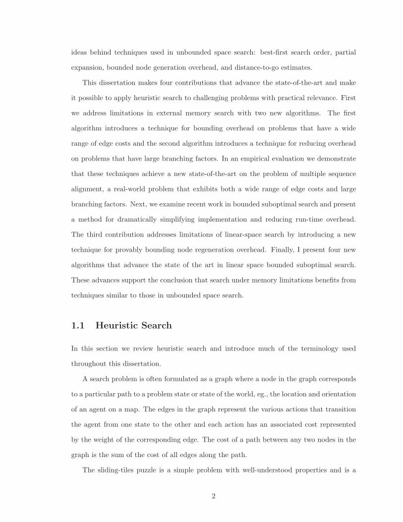
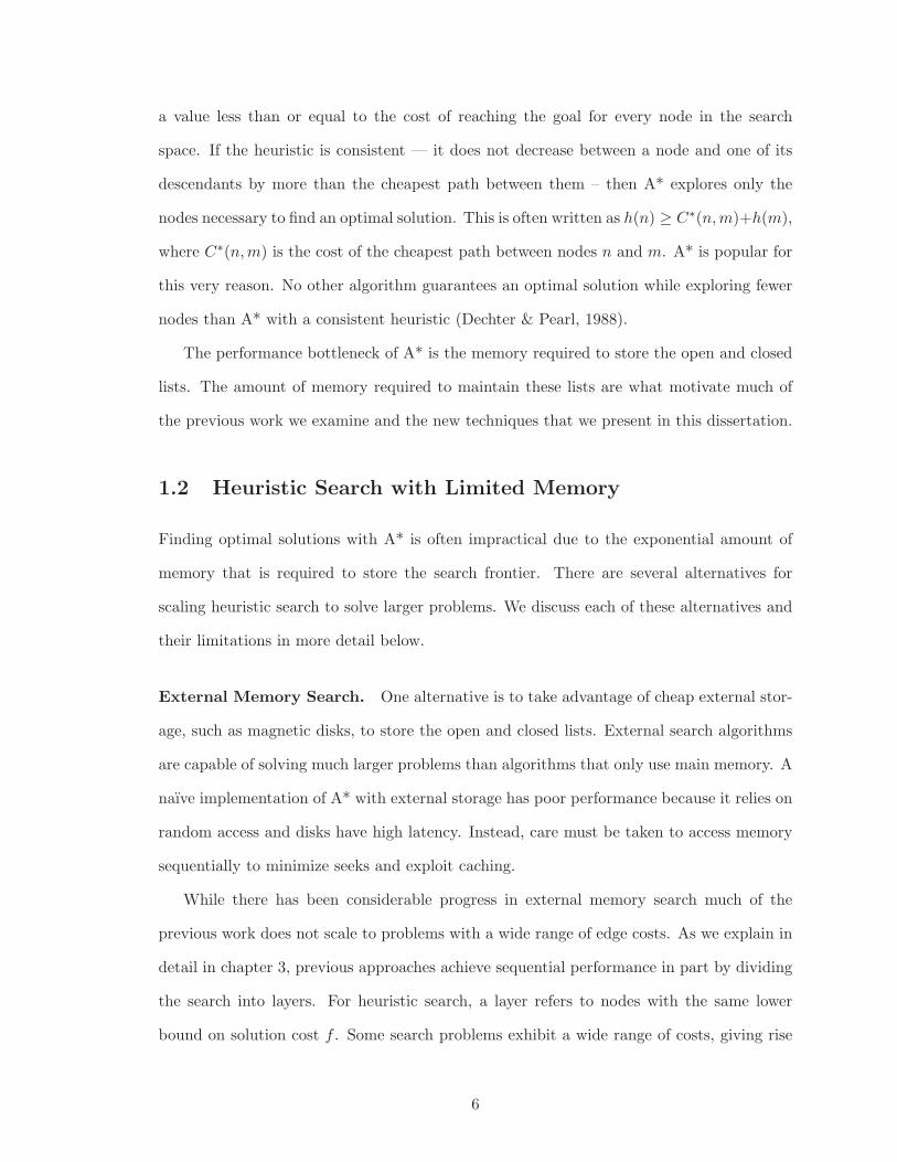
solutions, and this is what makes algorithms like A* so important. Figure 1-1 illustrates the

3

Breadth-First Search A* Search

start goalstart goal

Figure 1-1: A visual comparison of breadth-first search and A* search. Breadth-first search

explores a much larger portion of the search space while A* search explores only the portion

that appears most promising.

difference between a breadth-first search and A* search. The highlighted areas represent

the nodes expanded by each algorithm, the green circle represents the start state and the

star represents the goal. A* explores a much smaller portion of the graph.

What separates heuristic search from other graph-traversal algorithms is the use of

heuristics. A heuristic is a bit of knowledge — a rule of thumb — about a problem that

allows you to make better decisions. In the context of search algorithms, the term heuristic

has a specific meaning: a function that estimates the cost remaining to reach a goal from

a particular node. A* can take advantage of heuristics to avoid unnecessary computation

by deciding which nodes appear to be the most promising to explore. A* tries to avoid

exploring nodes in the graph that do not appear to lead to an optimal solution and can

often find solutions faster and with less memory than less-informed algorithms.

Starting from the initial node, A* proceeds by exploring the most promising nodes first.

All of the applicable actions are applied at each node, generating new successor nodes that

are then added to the list of unexplored nodes (also referred to as the frontier of the search).

4

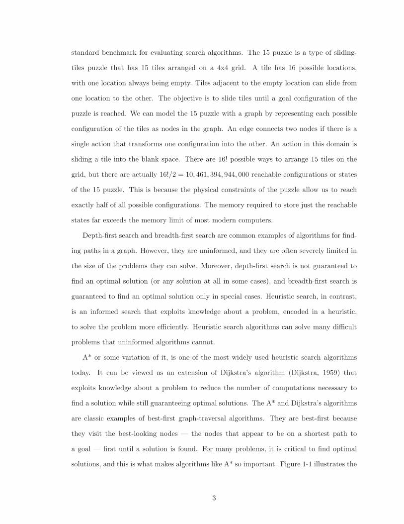
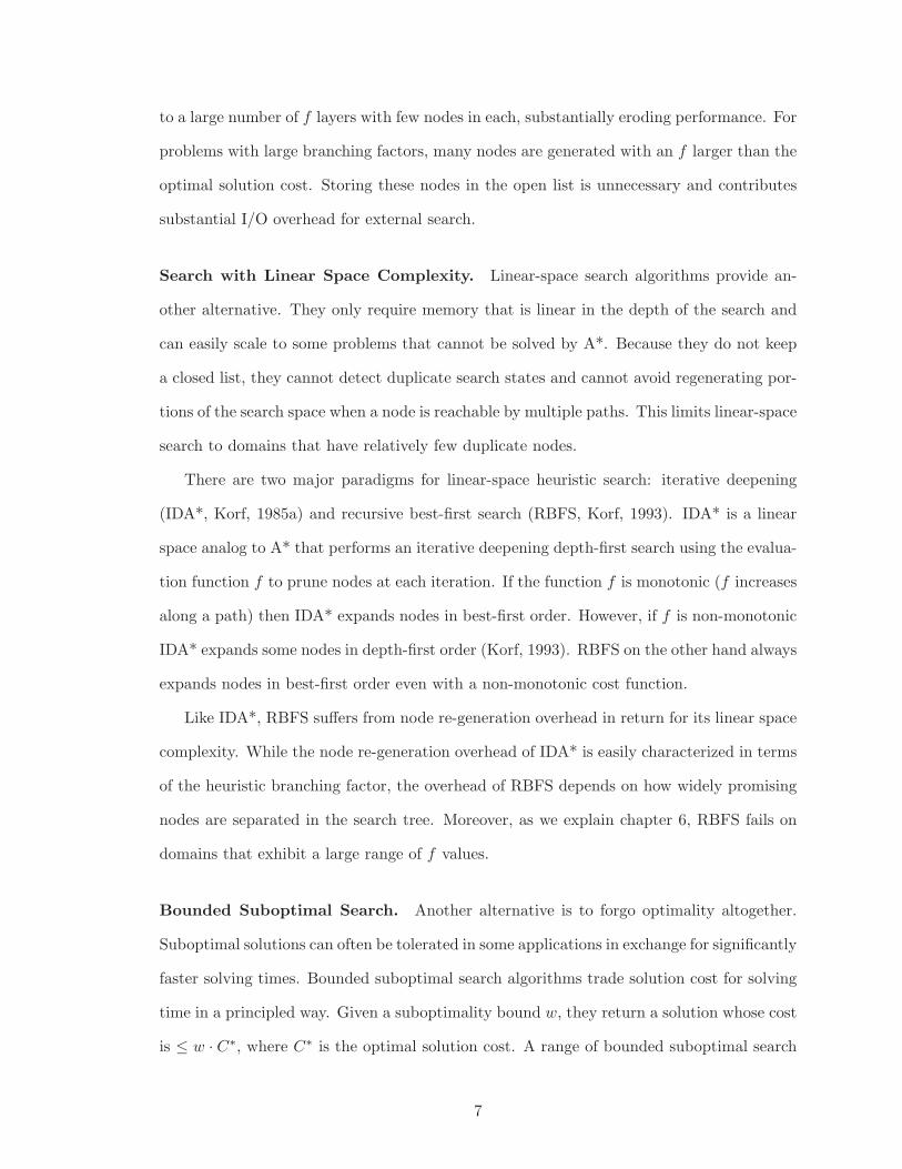
hg

Figure 1-2: A* orders the search using the evaluation function f(n) = g(n) + h(n). Nodes

with lower f are estimated to be on a cheaper path to the goal and thus, more promising

to explore.

The frontier is often stored in a data structure called the open list. The process of exploring

a node and generating all of its successor nodes is commonly referred to as expanding the

node. You can think of this search procedure as generating a tree: The tree’s root node

represents the initial state, and child nodes are connected by edges that represent the actions

that were used to generate them. To avoid regenerating the same states through multiple

paths, A* must store a copy of every state it has ever encountered. These are often stored in

a data structure called the closed list. Nodes that correspond to the same state are referred

to as duplicate nodes and the closed list is used to identify duplicate nodes. Originally the

closed list was intended to store nodes that have already been expanded. However, it is a

common optimization to store all generated states in the closed list.

To determine which nodes appear most promising, A* uses the evaluation function

f(n) = g(n) + h(n). This function estimates the cost of a solution through node n where

g(n) is the cost to reach node n from the initial state and h(n) is the estimated cost to

reach the goal from node n. The nodes with the lowest f values are the ones that appear

to be the most promising nodes to explore and thus the open list is often sorted by f .

If the heuristic is admissible — it never over estimates — then A* is guaranteed to find

an optimal solution. For the heuristic estimate to be admissible, it must be a lower bound:

5

a value less than or equal to the cost of reaching the goal for every node in the search

space. If the heuristic is consistent — it does not decrease between a node and one of its

descendants by more than the cheapest path between them – then A* explores only the

nodes necessary to find an optimal solution. This is often written as h(n) ≥ C∗(n,m)+h(m),

where C∗(n,m) is the cost of the cheapest path between nodes n and m. A* is popular for

this very reason. No other algorithm guarantees an optimal solution while exploring fewer

nodes than A* with a consistent heuristic (Dechter & Pearl, 1988).

The performance bottleneck of A* is the memory required to store the open and closed

lists. The amount of memory required to maintain these lists are what motivate much of

the previous work we examine and the new techniques that we present in this dissertation.

1.2 Heuristic Search with Limited Memory

Finding optimal solutions with A* is often impractical due to the exponential amount of

memory that is required to store the search frontier. There are several alternatives for

scaling heuristic search to solve larger problems. We discuss each of these alternatives and

their limitations in more detail below.

External Memory Search. One alternative is to take advantage of cheap external stor-

age, such as magnetic disks, to store the open and closed lists. External search algorithms

are capable of solving much larger problems than algorithms that only use main memory. A

naıve implementation of A* with external storage has poor performance because it relies on

random access and disks have high latency. Instead, care must be taken to access memory

sequentially to minimize seeks and exploit caching.

While there has been considerable progress in external memory search much of the

previous work does not scale to problems with a wide range of edge costs. As we explain in

detail in chapter 3, previous approaches achieve sequential performance in part by dividing

the search into layers. For heuristic search, a layer refers to nodes with the same lower

bound on solution cost f . Some search problems exhibit a wide range of costs, giving rise

6

to a large number of f layers with few nodes in each, substantially eroding performance. For

problems with large branching factors, many nodes are generated with an f larger than the

optimal solution cost. Storing these nodes in the open list is unnecessary and contributes

substantial I/O overhead for external search.

Search with Linear Space Complexity. Linear-space search algorithms provide an-

other alternative. They only require memory that is linear in the depth of the search and

can easily scale to some problems that cannot be solved by A*. Because they do not keep

a closed list, they cannot detect duplicate search states and cannot avoid regenerating por-

tions of the search space when a node is reachable by multiple paths. This limits linear-space

search to domains that have relatively few duplicate nodes.

There are two major paradigms for linear-space heuristic search: iterative deepening

(IDA*, Korf, 1985a) and recursive best-first search (RBFS, Korf, 1993). IDA* is a linear

space analog to A* that performs an iterative deepening depth-first search using the evalua-

tion function f to prune nodes at each iteration. If the function f is monotonic (f increases

along a path) then IDA* expands nodes in best-first order. However, if f is non-monotonic

IDA* expands some nodes in depth-first order (Korf, 1993). RBFS on the other hand always

expands nodes in best-first order even with a non-monotonic cost function.

Like IDA*, RBFS suffers from node re-generation overhead in return for its linear space

complexity. While the node re-generation overhead of IDA* is easily characterized in terms

of the heuristic branching factor, the overhead of RBFS depends on how widely promising

nodes are separated in the search tree. Moreover, as we explain chapter 6, RBFS fails on

domains that exhibit a large range of f values.

Bounded Suboptimal Search. Another alternative is to forgo optimality altogether.

Suboptimal solutions can often be tolerated in some applications in exchange for significantly

faster solving times. Bounded suboptimal search algorithms trade solution cost for solving

time in a principled way. Given a suboptimality bound w, they return a solution whose cost

is ≤ w · C∗, where C∗ is the optimal solution cost. A range of bounded suboptimal search

7

algorithms have been proposed, of which the best-known is Weighted A* (WA*, Pohl, 1973).

WA* is a best-first search using the f ′(n) = g(n) +w · h(n) evaluation function and is able

to solve problems faster than A* and with less memory.

WA* returns solutions with bounded suboptimality only when using an admissible cost-

to-go heuristic h(n). There has been much previous work over the past decade demon-

strating that inadmissible but accurate heuristics can be used effectively to guide search

algorithms (Jabbari Arfaee, Zilles, & Holte, 2011; Samadi, Felner, & Schaeffer, 2008). In-

admissible heuristics can even be learned online (Thayer, Dionne, & Ruml, 2011). Further-

more, recent work has shown that WA* can perform very poorly in domains where the costs

of the edges are not uniform (Wilt & Ruml, 2012). In such domains, an estimate of the

minimal number of actions needed to reach a goal can be utilized as an additional heuristic

to effectively guide the search to finding solutions quickly.

Unfortunately, incorporating these additional heuristics requires that the search syn-

chronize multiple priority queues, resulting in lower node expansion rates than single queue

algorithms such as WA*. As we explain further in chapter 5, it is possible to reduce some

of the overhead by employing complex data structures. However, as our results show, sub-

stantial overhead remains and it is possible for WA* to outperform these algorithms when

distance-to-go estimates and inadmissible heuristics do not provide enough of an advantage

to overcome this inefficiency.

Bounded Suboptimal Search in Linear Space. While bounded suboptimal search

algorithms scale to problems that cannot be solved optimally, for large problems or tight

suboptimality bounds, they can still overrun memory. It is possible to combine linear-space

search with bounded suboptimal search to solve problems that cannot be solved by either

method alone. Weighted IDA* (WIDA*, Korf, 1993) is a bounded suboptimal variant of

IDA* that uses the non-monotonic cost function of WA*. Unfortunately, because linear-

space search algorithms are based on iterative deepening depth-first search they are not

able to incorporate distance-to-go estimates directly, which have been shown to give state-

of-the-art performance.

8

1.3 Real-World Problems

Some of the techniques mentioned in the previous section are limited to problems that do

not exhibit certain properties that are often found in real-world problems. In this section

we discuss these in more detail.

Non-uniform Edge Costs. Many toy problems such as the sliding-tiles puzzle, Rubik’s

cube and Towers of Hanoi are commonly studied domains for heuristic search algorithms.

These problems are useful because they are simple to reproduce and have well understood

properties. For example all actions have the same cost and as a result all edges in the

search graph have the same weight, giving rise to a small range of possible f values. In

contrast, many real-world problems have a wide variety of edge costs, resulting in many

possible f values. In the most extreme case each node on the search frontier may have a

unique f value. Unfortunately, previous algorithms fail on domains that have non-uniform

edge costs. For example, IDA* expands O(n) nodes on domains where the number of nodes

with the same f exhibits geometric growth, where n is the number of nodes expanded by

A* to find an optimal solution. This geometric growth is common in domains that have

uniform edge costs. However, when the domain does not exhibit this geometric growth, the

number of new nodes expanded in each iteration is constant, and IDA* can expand O(n2)

nodes.

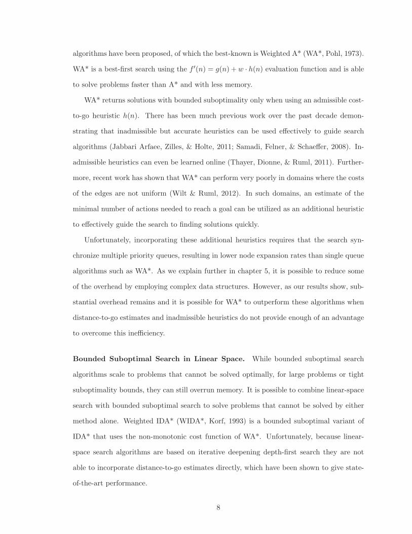
Figure 1-3 shows two search spaces, one with uniform edge costs and the other with

non-uniform edge costs. The search space with uniform edge costs has just 3 different f

values, IDA* would need to perform just 3 iterations and a total of 17 node expansions

to explore this space. The search space on the right has 10 different f values, each node

having a unique value. IDA* would need to perform 10 iterations and a total of 55 node

expansions to explore this space. As we show in chapter 6, RBFS also suffers on domains

that exhibit a wide range of edge costs.

Fringe search (Bjornsson, Enzenberger, Holte, & Schaeffer, 2005), a variant of A* that

stores the open list in a linked list instead of a priority queue, also fails on domains with

9

Uniform Costs Non-Uniform Costs

f = 3

f = 5

f = 7

f=3.3

f=6.8

f=5.1 f=5.3

f=7.7

f=3.4

f=7.5

f=7.2 f=7.3

f=7.6

Figure 1-3: The search space on the left has uniform edge costs, resulting in just 3 different

f layers. The search space on the right has non-uniform costs, resulting in 10 f layers, one

layer for each node.

non-uniform costs. At each iteration, Fringe search performs a linear scan of the open list

and expands previously unexplored nodes with the same minimum f value. In the worst

case, each node has a unique f value, and Fringe search incurs significant overhead as it has

to scan the entire linked list to expand just a single node at each iteration. External search

algorithms use a similar f -layered based search procedure and fail for the same reason. We

examine this issue in more detail in chapter 3.

Large Branching Factors. Another property common to many real-world search prob-

lems is that they have large branching factors: there are many possible actions to take from

any given state. For these problems the search frontier grows rapidly and can exhaust the

memory available on most modern computers in a matter of seconds. Moreover, a significant

portion of the nodes on the open list are never explored because their f values are larger

than the cost of an optimal solution. Storing these nodes on the open list is unnecessary

and wastes valuable memory.

Multiple sequence alignment (MSA), a search problem with practical relevance, has a

very large branching factor, O(2k) where k is the number of sequences being aligned, and

a very wide range of f values. For example, the maximum branching factor when aligning

just 8 sequences is 28 − 1 = 255. That is, each time a node is expanded a maximum of 255

successor nodes may be placed on the open list. The open list for this problem grows very

10

rapidly with search progress, much faster than toy domains, like the sliding tiles puzzle,

and algorithms such as A* fail to solve these problems because of the memory requirements

to store the open list. Moreover, many of the nodes on the open list can have an estimated

solution cost f > f∗. These nodes are never expanded by an A* search and storing them is

not necessary to guarantee optimal solutions. We study MSA in more detail in chapter 4.

Distance-to-go Estimates. Another common property of real-world problems is that

shortest paths (paths containing the fewest edges) are not always equivalent to least-cost

paths (paths whose edges sum to the minimal cost among all other paths). When the

problem exhibits non-uniform costs, a least-cost path may actually be longer (contain more

edges) than more costly paths. We refer to the estimate of the number of edges that

separate a node from a goal as the node’s distance-to-go. In domains with uniform costs

this is often equivalent to the heuristic cost-to-go estimate of the node. However, in domains

with non-uniform costs distance-to-go estimates differ from cost-to-go estimates and often

provide additional search guidance. The distance-to-go estimate can act as a proxy for the

number of nodes that need to be expanded below a node in order to reach a goal. Pursuing

the nodes that are estimated to be closer to the goal may require less effort — fewer node

expansions — by the search algorithm, resulting in faster solving times.

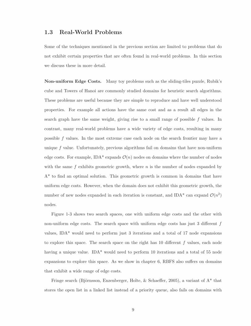
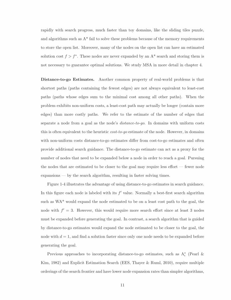
Figure 1-4 illustrates the advantage of using distance-to-go estimates in search guidance.

In this figure each node is labeled with its f ′ value. Normally a best-first search algorithm

such as WA* would expand the node estimated to be on a least cost path to the goal, the

node with f ′ = 3. However, this would require more search effort since at least 3 nodes

must be expanded before generating the goal. In contrast, a search algorithm that is guided

by distance-to-go estimates would expand the node estimated to be closer to the goal, the

node with d = 1, and find a solution faster since only one node needs to be expanded before

generating the goal.

Previous approaches to incorporating distance-to-go estimates, such as A∗

ǫ (Pearl &

Kim, 1982) and Explicit Estimation Search (EES, Thayer & Ruml, 2010), require multiple

orderings of the search frontier and have lower node expansion rates than simpler algorithms,

11

44

3

45

d=1d=3

Figure 1-4: A search space where distance-to-go estimates provide search guidance. Best-

first search would normally expand the node estimated to have least cost f = 3. However,

this would require more search effort than expanding the node estimated to be closer to the

goal d = 1.

such as WA*, because of the overhead of maintaining multiple priority queues. Incorporating

distance-to-go estimates must provide enough of an advantage to overcome this inefficiency

for these algorithms or they perform no better than WA*. Moreover, it is not obvious how

linear-space algorithms, which are based on depth-first search, can incorporate distance-to-

go estimates. We examine both of these issues in more detail in chapters 5 and 7.

1.4 Dissertation Outline

This dissertation is organized into eight chapters including an introduction and conclusion.

We summarize each of the remaining chapters below.

Chapter 2: External Search

In this chapter we motivate the use of external memory for heuristic search. We describe

the techniques of Delayed Duplicate Detection (DDD) and Hash-Based DDD (HBDDD) in

12

detail and present an empirical study of a parallel external memory variant of A* (A*-DDD).

Chapter 3: External Search: Non-Uniform Edge Costs

In this chapter we investigate previously proposed algorithms that fail on problems that

exhibit a wide range of edge costs. We examine this limitation in detail and present a

new parallel external memory search algorithm that is capable of solving problems with

arbitrary edge costs. This work was published in AAAI-2011.

Chapter 4: External Search: Large Branching Factors

Many real-world problems such as Multiple Sequence Alignment (MSA) have high branch-

ing factors leading to rapidly growing frontiers and for some problems many of the nodes on

the frontier are never expanded. In the third chapter we introduce MSA and describe how

previous algorithms do not scale because of MSA’s large branching factor. A new best-first

external search algorithm, that is designed specifically for dealing with large branching fac-

tors, is presented and applied to the challenging problem of MSA. This work was published

in AAAI-2013.

Chapter 5: Bounded Suboptimal Search

One way to speed up search is to relax the optimality requirement. Problems that take

hours or days when solved optimally can be solved in seconds using suboptimal search. In

this chapter we take a departure from optimal search and present an iterative deepening

approach to dramatically simplify and boost the performance of state-of-the-art bounded

suboptimal search. This approach also provides a foundation for algorithms introduced

later chapter 7. This work is currently under review for publication.

Chapter 6: Heuristic Search in Linear Space

In this chapter we investigate algorithms with linear space complexity. We show that

some linear-space algorithms, like previously proposed external search algorithms, fail on

13

domains that have a wide range of edge costs. To this end, we introduce the first best-first

linear-space search technique for provably bounding overhead and solving problems with

non-uniform edge costs. This work is currently under review for publication.

Chapter 7: Bounded Suboptimal Search in Linear Space

In this chapter we investigate techniques for combining the ideas behind state-of-the-art

bounded suboptimal search, such as incorporating inadmissible heuristics and solution

length estimates, with linear-space search to solve problems that cannot be solved with

either technique alone. Part of this work was published in SoCS-2013 and the remaining

work is currently under review for publication.

Chapter 8: Conclusion

This chapter concludes the dissertation with a summary of the contributions presented in

each chapter.

14

CHAPTER 2

EXTERNAL MEMORY SEARCH

2.1 Introduction

Best-first graph search algorithms such as A* (Hart et al., 1968) are widely used for solving

problems in artificial intelligence. Graph search algorithms typically maintain an open list,

containing nodes that have been generated but not yet expanded, and a closed list, contain-

ing all generated states, in order to prevent duplicated search effort when the same state

is generated via multiple paths. As the size of problems increases, however, the memory

required to maintain the open and closed lists makes algorithms like A* impractical. For ex-

ample, a sliding tiles puzzle solver that uses A* will exhaust 8 GB of RAM in approximately

2 minutes on a machine with a dual-core 3.16 GHz processor.

External memory search algorithms take advantage of cheap secondary storage, such as

magnetic disks, to solve much larger problems than algorithms that only use main memory.

A naıve implementation of A* with external storage has poor performance because it relies

on random access and disks have high latency. Instead, great care must be taken to access

memory sequentially to minimize seeks and exploit caching. The same techniques used for

external memory search may also be used to take advantage of multiple processors and

overcome the latency of disk with parallel search.

There are two popular techniques for external memory search, Delayed Duplicate Detec-

tion (DDD, Korf, 2003) and Structured Duplicate Detection (SDD, Zhou & Hansen, 2004).

DDD writes newly generated nodes to disk and defers the process of duplicate detection to

a later phase. In contrast, SDD uses a projection function to localize memory references

and performs duplicate merging immediately in main memory. Unlike DDD, SDD does not

store duplicate states to disk and requires less external storage. However, this efficiency

15

comes at the cost of increased time complexity and SDD can read and write the same states

multiple times during duplicate processing (Zhou & Hansen, 2009).

In this chapter we discuss the technique of delayed duplicate detection in detail and

present empirical results for an efficient external memory variant of A* (A*-DDD). As far

as we are aware, we are the first to present results for HBDDD using A* search, other than

the anecdotal results mentioned briefly by Korf (2004). These results provide evidence that

A*-DDD performs well on unit-cost domains and that efficient parallel external memory

search can surpass serial in-memory search.

2.2 Delayed Duplicate Detection

One simple way to make use of external storage for graph search is to place newly generated

nodes in external memory and then process them at a later time. There are two forms of

DDD, sorting-based DDD and hash-based DDD. We discuss both in more detail below.

2.2.1 Sorting-Based Delayed Duplicate Detection

Sorting-based DDD search divides the search process into two phases, an expand phase and

a merge phase. The expand phase writes newly generated nodes directly to a file on disk.

Each state is given a unique lexicographic hash. The merge phase performs a disk-based sort

on the file so that duplicate nodes are brought together. Duplicate merging is accomplished

by performing a linear scan of the sorted file, writing each unique node to a new file on

disk. This newly merged file becomes the search frontier for the next expand phase.

This technique has the advantage of having minimal memory requirements. To perform

search, only a single node needs to fit in main memory. Unfortunately the time complexity

of this technique is O(n log n) where n is the total number of nodes encountered during

search. For really large problems this technique incurs more overhead than is desirable. In

the next section we discuss a technique that achieves linear-time complexity at the cost of

increased space complexity.

16

2.2.2 Hash-Based Delayed Duplicate Detection

To avoid the overhead of disk-based sorting, Korf (2008) presents an efficient form of this

technique called Hash-Based Delayed Duplicate Detection (HBDDD). HBDDD uses two

hash functions, one to assign nodes to buckets (which map to files on disk) and a second

hash function to identify duplicate states within a bucket. Because duplicate nodes will hash

to the same value, they will always be assigned to the same file. When removing duplicate

nodes, only those nodes in the same file need to be in main memory. This technique increases

the space complexity over sorting-based DDD, requiring that the size of the largest bucket

fit in main memory.

Korf (2008) described how HBDDD can be combined with A* search (A*-DDD). In the

expansion phase, all nodes that an f that is equal to the minimum solution cost estimate

fmin of all open nodes are expanded. The expanded nodes and the newly generated nodes

are stored in their respective files. If a generated node has an f ≤ fmin, then it is expanded

immediately instead of being stored to disk. This is called a recursive expansion. Once all

nodes within fmin are expanded, the merge phase begins: each file is read into a hash-table

in main memory and duplicates are removed in linear time. During the expand phase,

HBDDD requires only enough memory to read and expand a single node from the open

file; successors can be stored to disk immediately. During the merge phase, it is possible

to process a single file at a time. One requirement for HBDDD is that all nodes in the

largest file fit in main memory. This is easily achieved by using a hash function with an

appropriate range.

HBDDD may also be used as a framework to parallelize search (PA*-DDD, Korf, 2008).

Because duplicate states will be located in the same file, the merging of delayed duplicates

can be done in parallel, with each file assigned to a different thread. Expansion may also

be done in parallel. As nodes are generated, they are stored in the file specified by the hash

function. It is possible for two threads to generate nodes that need to be placed in the same

file. Therefore, a lock (often provided by the OS) must be placed around each file. For our

experiments we verified that a lock was provided by examining the source code for the I/O

17

modules. For example, the source code for the glibc standard library 2.12.90 does contain

such a lock.

2.3 Parallel External A*

The contributions of chapters 3 and 4 build on the framework of A*-DDD. In this section

we discuss A*-DDD in detail and present empirical results.

A*-DDD proceeds in two phases: an expansion phase and a merge phase. Search nodes

are mapped to buckets using a hash function. Each bucket is backed by a set of three files

on disk: 1) a file of frontier nodes that have yet to be expanded, 2) a file of newly generated

nodes (and possibly duplicates) that have yet to be checked against the closed list and 3) a

file of closed nodes that have already been expanded. During the expansion phase, A*-DDD

expands the set of frontier nodes that have an f = fmin and recursively, any newly generated

nodes with f ≤ fmin.

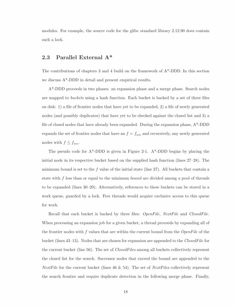
The pseudo code for A*-DDD is given in Figure 2-1. A*-DDD begins by placing the

initial node in its respective bucket based on the supplied hash function (lines 27–28). The

minimum bound is set to the f value of the initial state (line 27). All buckets that contain a

state with f less than or equal to the minimum bound are divided among a pool of threads

to be expanded (lines 30–20). Alternatively, references to these buckets can be stored in a

work queue, guarded by a lock. Free threads would acquire exclusive access to this queue

for work.

Recall that each bucket is backed by three files: OpenFile, NextFile and ClosedFile.

When processing an expansion job for a given bucket, a thread proceeds by expanding all of

the frontier nodes with f values that are within the current bound from the OpenFile of the

bucket (lines 43–13). Nodes that are chosen for expansion are appended to the ClosedFile for

the current bucket (line 56). The set of ClosedFiles among all buckets collectively represent

the closed list for the search. Successor nodes that exceed the bound are appended to the

NextFile for the current bucket (lines 46 & 54). The set of NextFiles collectively represent

the search frontier and require duplicate detection in the following merge phase. Finally,

18

Search(initial)1. bound ← f (initial); bucket ← hash(initial)2. write(OpenFile(bucket), initial)3. while ∃bucket ∈ Buckets : min f (bucket) ≤ bound4. for each bucket ∈ Buckets : min f (bucket) ≤ bound5. ThreadExpand(bucket)6. if incumbent break7. for each bucket ∈ Buckets : NeedsMerge(bucket)8. ThreadMerge(bucket)9. bound ← min f (Buckets)

ThreadExpand(bucket)10. for each state ∈ Read(OpenFile(bucket))11. if f (state) ≤ bound12. RecurExpand(state)13. else append(NextFile(bucket), state)

RecurExpand(n)14. if IsGoal(n) incumbent ← n; return15. for each succ ∈ expand(n)16. if f (succ) ≤ bound17. RecurExpand(succ)18. else19. append(NextFile(hash(succ)), succ)20. append(ClosedFile(hash(n)),n)

ThreadMerge(bucket)21. Closed ← read(ClosedFile(bucket)); Open ← ∅22. for each n ∈ NextFile(bucket)23. if n /∈ Closed ∪Open or g(n) < g(Closed ∪Open[n])24. Open ← (Open −Open[n]) ∪ {n}25. write(OpenFile(bucket), Open)26. write(ClosedFile(bucket), Closed)

Figure 2-1: Pseudocode for A*-DDD.

19

if a successor is generated with an f value that is within the current bound then it is

expanded immediately as a recursive expansion (lines 45 & 52). States are not written to

disk immediately upon generation. Instead each bucket has an internal buffer to hold states.

When the buffer becomes full, the states are written to disk.

If an expansion thread generates a goal state (line 47) a reference to the incumbent

solution is created and the search terminates (line 32). Assuming the heuristic is admissible,

then the incumbent is admissible because of the strict best-first search order on f . Otherwise

a branch-and-bound procedure would be required when expanding the final f layer. If a

solution has not been found, then all buckets that require merging are divided among a

pool of threads to be merged in the next phase (lines 33–34).

In order to process a merge job, each thread begins by reading the ClosedFile for the

bucket into a hash-table (line 36) called Closed . A*-DDD requires enough memory to store

all closed nodes in all buckets being merged. The size of a bucket can be easily tuned by

varying the granularity of the hash function. Next all frontier nodes in the NextFile are

streamed in and checked for duplicates against the closed list (lines 37–42). The nodes

that are not duplicates or that have been reached via a better path are written back out to

NextFile so that they remain on the frontier for latter phases of search (lines 38–41). All

other duplicate nodes are ignored.

To save external storage with HBDDD, Korf (2008) suggests that instead of proceeding

in two phases, merges may be interleaved with expansions. With this optimization, a

bucket may be merged if all of the buckets that contain its predecessor nodes have been

expanded. An undocumented ramification of this optimization, however, is that it does

not permit recursive expansions. Because of recursive expansions, one cannot determine

the predecessor buckets and therefore all buckets must be expanded before merges can

begin. A*-DDD uses recursive expansions and therefore it does not interleave expansions

and merges.

20

2.4 Empirical Results

We evaluated the performance of A*-DDD on the sliding tiles puzzle. To verify that we had

efficient implementations of these algorithms, we compared our implementations (in Java)

to highly optimized versions of A* and IDA* written in C++ (Burns, Hatem, Leighton, &

Ruml, 2012). The Java implementations use many of the same optimizations. In addition

we use the High Performance Primitive Collection (HPPC) in place of the Java Collections

Framework (JCF) for many of our data structures. This improves both the time and memory

performance of our implementations (Hatem, Burns, & Ruml, 2013).

We compared A*-DDD with internal A*, IDA* and Asynchronous Parallel IDA* (AIDA*,

Reinefeld & Schnecke, 1994). AIDA* is a parallel version of IDA* that works by performing

a breadth-first search to some specified depth and the resulting frontier is then divided

evenly among all available threads. Threads perform an IDA* search in parallel for each

node in its queue. The upper bounds for all IDA* searches are synchronized across all

threads so that a strict best-first search order is achieved given an admissible and consis-

tent heuristic.

We also compared A*-DDD to an alternative external algorithm, breadth-first heuristic

search (BFHS, Zhou & Hansen, 2006) with delayed duplicate detection. BFHS is a reduced

memory search algorithm that attempts to reduce the memory requirement of search, in

part by removing the need for a closed list. BFHS proceeds in a breadth-first ordering by

expanding all nodes within a given upper bound on f at one depth before proceeding to the

next depth. To prevent duplicate search effort Zhou and Hansen (2006) prove that, in an

undirected graph, checking for duplicates against the previous depth layer and the frontier

is sufficient to prevent the search from leaking back into previously visited portions of the

space. While BFHS is able to do away with the closed list, for many problems it will still

require a significant amount of memory to store the exponentially growing search frontier.

BFHS uses an upper bound on f values to prune nodes. If a bound is not available in

advance, iterative deepening can be used. However, as discussed earlier, this technique fails

on domains with many distinct f values. Also, since BFHS does not store a closed list, the

21

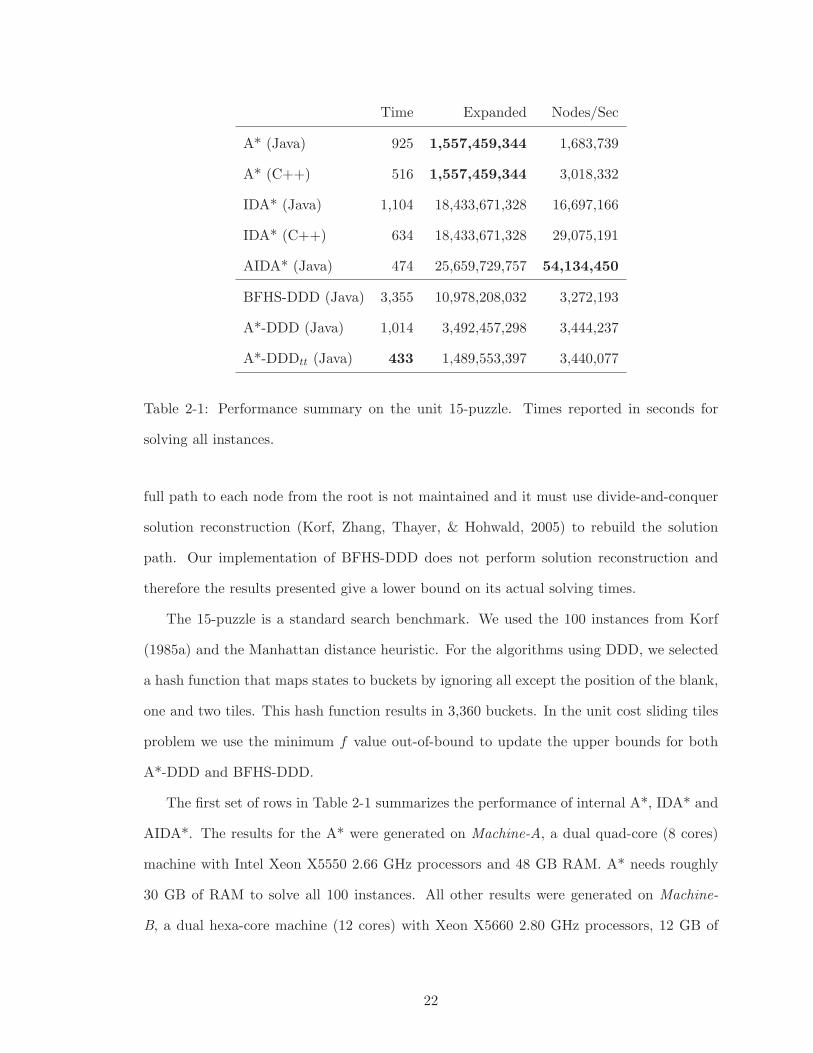
Time Expanded Nodes/Sec

A* (Java) 925 1,557,459,344 1,683,739

A* (C++) 516 1,557,459,344 3,018,332

IDA* (Java) 1,104 18,433,671,328 16,697,166

IDA* (C++) 634 18,433,671,328 29,075,191

AIDA* (Java) 474 25,659,729,757 54,134,450

BFHS-DDD (Java) 3,355 10,978,208,032 3,272,193

A*-DDD (Java) 1,014 3,492,457,298 3,444,237

A*-DDDtt (Java) 433 1,489,553,397 3,440,077

Table 2-1: Performance summary on the unit 15-puzzle. Times reported in seconds for

solving all instances.

full path to each node from the root is not maintained and it must use divide-and-conquer

solution reconstruction (Korf, Zhang, Thayer, & Hohwald, 2005) to rebuild the solution

path. Our implementation of BFHS-DDD does not perform solution reconstruction and

therefore the results presented give a lower bound on its actual solving times.

The 15-puzzle is a standard search benchmark. We used the 100 instances from Korf

(1985a) and the Manhattan distance heuristic. For the algorithms using DDD, we selected

a hash function that maps states to buckets by ignoring all except the position of the blank,

one and two tiles. This hash function results in 3,360 buckets. In the unit cost sliding tiles

problem we use the minimum f value out-of-bound to update the upper bounds for both

A*-DDD and BFHS-DDD.

The first set of rows in Table 2-1 summarizes the performance of internal A*, IDA* and

AIDA*. The results for the A* were generated on Machine-A, a dual quad-core (8 cores)

machine with Intel Xeon X5550 2.66 GHz processors and 48 GB RAM. A* needs roughly

30 GB of RAM to solve all 100 instances. All other results were generated on Machine-

B, a dual hexa-core machine (12 cores) with Xeon X5660 2.80 GHz processors, 12 GB of

22

RAM and 12 320 GB disks. AIDA* used 24 threads. From these results, we see that the

Java implementation of A* is just a factor of 1.7 slower than the most optimized C++

implementation known. These results provide confidence that our comparisons reflect the

true ability of the algorithms rather than misleading aspects of implementation details.

The second set of rows in Table 2-1 shows a summary of the performance results for

A*-DDD compared to in-memory search. We used 24 threads and the states generated

by A*-DDD and BFHS-DDD were distributed across all 12 disks. A*-DDD outperforms

BFHS-DDD because it expands fewer nodes. We discuss this in more detail in chapter 3. In-

memory A* is not able to solve all 100 instances on this machine due to memory constraints.

We compare A*-DDD to Burns et al.’s highly optimized IDA* solver implemented in C++

(Burns et al., 2012) and a similarly optimized IDA* solver in Java. The results show that

the base Java implementation of A*-DDD is just 1.7× slower than the C++ implementation

of IDA* but faster than the Java implementation. We can improve the performance of A*-

DDD with the simple technique of using transposition tables to avoid expanding duplicate

states during recursive expansions (A*-DDDtt). With this improvement A*-DDD is 1.4×

faster than the highly optimized C++ IDA* solver and 2.5× faster than the optimized Java

IDA* solver. A*-DDDtt is even slightly faster than AIDA*.

2.5 Discussion

In this section we discuss the limitations of A*-DDD that motivate the next two chapters.

2.5.1 Non-Uniform Edge Costs

A*-DDD works by dividing the search into f layers. While our results have shown that

A*-DDD works well on domains with unit edge costs such as the the sliding tiles puzzle,

it suffers from excessive I/O overhead on domains that exhibit many unique f values. A*-

DDD reads all open nodes from files on disk and expands only the nodes within the current

f bound. If there are a small number of nodes in each f layer, the algorithm pays the cost of

reading the entire frontier only to expand a few nodes. Then in the merge phase, the entire

23

closed list is read only to merge the same few nodes. Additionally, when there are many

distinct f values, the successors of each node tend to exceed the current f bound, resulting

in fewer I/O-efficient recursive expansions. Korf (2004) speculated that the problem of many

distinct f values could be remedied by somehow expanding more nodes than just those with

the minimum f value. In chapter 3 we present a new algorithm that does exactly this.

2.5.2 Large Branching Factors

The branching factor for the sliding-tile puzzles are relatively small since there are few

actions that can be taken from any state. Each time a node is expanded the search generates

at most 3 new nodes, 4 if you include regenerating the parent node. On domains such as

multiple sequence alignment, there can be many actions to take at every state, resulting

in a rapidly increasing search frontier. For domains with practical relevance, these actions

can take on a wide range of costs and many of the new nodes that are generated are never

expanded by the search because their costs exceed the cost of an optimal solution. For

external memory search this results in a lot of wasted I/O overhead as these nodes that

are never expanded are read from and written to disk at each iteration of the search. This

limitation motivates the work presented in chapter 4.

2.6 Conclusion

In this chapter we discussed techniques for external memory search in detail. We described

an efficient external memory variant of A* (A*-DDD) and presented empirical results for

the sliding tiles puzzle, comparing A*-DDD with internal memory search algorithms and an

alternative external memory algorithm that relies on a breadth-first search strategy. These

results provide evidence that external memory search benefits from a best-first search order

and performs well on unit-cost domains and that efficient parallel external memory search

can surpass serial in-memory search.

24

CHAPTER 3

EXTERNAL MEMORY SEARCH WITH

NON-UNIFORM EDGE COSTS

3.1 Introduction

External memory search algorithms take advantage of cheap secondary storage, such as

magnetic disks, to solve much larger problems than algorithms that only use main memory.

As we discussed in chapter 2, previous approaches achieve sequential performance in part

by dividing the search into layers. For heuristic search, a layer refers to nodes with the

same lower bound on solution cost f . Many real-world problems have real-valued costs,

giving rise to a large number of f layers with few nodes in each, substantially eroding

performance. The main contribution of this chapter is a new strategy for external memory

search that performs well on graphs with real-valued edges. Our new approach, Parallel

External search with Dynamic A* Layering (PEDAL), combines A* with hash-based delayed

duplicate detection (HBDDD, Korf, 2008), however we relax the best-first ordering of the

search in order to perform a constant number of expansions per I/O.

We compare PEDAL to IDA*, IDA*CR (Sarkar, Chakrabarti, Ghose, & Sarkar, 1991), A*

with hash-based delayed duplicate detection (A*-DDD) and breadth-first heuristic search

(Zhou & Hansen, 2006) with delayed duplicate detection (BFHS-DDD) using two variants

of the sliding-tile puzzle and a more realistic dockyard planning domain. The results show

that PEDAL gives the best performance on the sliding-tile puzzle and is the only practical

approach for the real-valued problems among the algorithms tested in our experiments.

PEDAL advances the state of the art by demonstrating that heuristic search can be effective

for large problems with real-valued costs.

25

3.2 Previous Work

In this section we present relevant previous work that PEDAL builds on and alternative

techniques.

3.2.1 Iterative Deepening A*

Iterative-deepening A* (IDA*, Korf, 1985a) is an internal memory technique that requires

memory only linear in the maximum depth of the search. This reduced memory complexity

comes at the cost of repeated search effort. IDA* performs iterations of a bounded depth-

first search where a path is pruned if f(n) becomes greater than the bound for the current

iteration. After each unsuccessful iteration, the bound is increased to the minimum f value

among the nodes that were generated but not expanded in the previous iteration.

Each iteration of IDA* expands a super-set of the nodes in the previous iteration. If

the size of iterations grows geometrically, then the number of nodes expanded by IDA*

is O(n), where n is the number of nodes that A* would expand (Sarkar et al., 1991). In

domains with real-valued edge costs, there can be many unique f values and the standard

minimum-out-of-bound bound schedule of IDA* may lead to only a few new nodes being

expanded in each iteration. The number of nodes expanded by IDA* can be O(n2) (Sarkar

et al., 1991) in the worst case when the number of new nodes expanded in each iteration

is constant. To alleviate this problem, Sarkar et al. introduce IDA*CR. IDA*CR tracks

the distribution of f values of the pruned nodes during an iteration of search and uses it

to find a good threshold for the next iteration. This is achieved by selecting the bound

that will cause the desired number of pruned nodes to be expanded in the next iteration.

If the successors of these pruned nodes are not expanded in the next iteration then this

scheme is often able to accurately double the number of nodes between iterations. If the

successors do fall within the bound on the next iteration then more nodes may be expanded

than desired. Since the threshold is increased liberally, nodes are not expanded in a strict

best-first order. Therefore, branch-and-bound must be used on the final iteration of search

to ensure optimality.

26

While IDA*CR can perform well on domains with real-valued edge costs by reducing the

number of times a node is regenerated, its estimation technique may fail to properly grow

the iterations in some domains. Moreover, IDA* suffers from an additional source of node

regeneration overhead on search spaces that form highly connected graphs. Because it uses

depth-first search, it cannot detect duplicate search states except those that form cycles

in the current search path. Even with cycle checking, the search will perform extremely

poorly if there are many paths to each node in the search space. This motivates the use of

a closed list in classic algorithms like A*.

3.2.2 Breadth-First Heuristic Search

Breadth-first heuristic search was described in the previous chapter but we include the

description in this chapter with further details. BFHS is a reduced memory search algorithm

that attempts to reduce the memory requirement of search, in part by removing the need

for a closed list. BFHS proceeds in a breadth-first ordering by expanding all nodes within

a given upper bound on f at one depth before proceeding to the next depth. To prevent

duplicate search effort Zhou and Hansen (2006) prove that, in an undirected graph, checking

for duplicates against the previous depth layer and the frontier is sufficient to prevent the

search from leaking back into previously visited portions of the space. While BFHS is able

to do away with the closed list, for many problems it will still require a significant amount

of memory to store the exponentially growing search frontier. Since BFHS does not store

a closed list, the full path to each node from the root is not maintained and it must use

divide-and-conquer solution reconstruction (Korf et al., 2005) to rebuild the solution path.

BFHS uses an upper bound on f values to prune nodes. If a bound is not available

in advance, iterative deepening can be used, however, as discussed earlier, this technique

fails on domains with many distinct f values. In this chapter we propose a novel variant

of BFHS that uses the same technique of IDA*CR for updating the upper bound at each

iteration of search.

One side effect of a breadth-first search order is that BFHS is not able to break ties

27

Best-First Search Order BFHS Search Order

5

6 7

7 6

7*

5

6 7

7 6

7*

5

6 7

7 6

7*

Figure 3-1: An example search tree showing the difference between a best-first search with

optimal tie-breaking and BFHS. The middle figure highlights the nodes (labeled with their

f values) expanded by a best-first search with optimal tie breaking and the figure on the

right highlights the nodes expanded by BFHS. BFHS must expand all nodes that have an

f equal to the optimal solution cost, and is equivalent to best-first search with worst-case

tie-breaking.

among nodes with the same f . In fact, the search order of BFHS is equivalent to A*

with worst-case tie breaking and can expand up to two times as many unique nodes as

A* with optimal tie breaking. Figure 3-1 illustrates this issue. The figure on the left

shows an example of a search tree with nodes labeled with their f values. A* with optimal

tie-breaking expands nodes with higher g values first (deeper nodes first in domains with

uniform edge costs). BFHS search needs to expand all nodes n with f(n) ≤ C∗ at all

depth-layers prior to the depth layer that contains the goal. This is equivalent to best-first

search with worst-case tie-breaking.

When combined with iterative deepening, BFHS can expand up to four times as many

nodes. Moreover, when combined with the bound setting technique of IDA*CR, it can

expand many nodes with f values greater than the optimal solution cost which are not

strictly necessary for optimal search. BFHS is not able to benefit from branch-and-bound

in the final iteration because goal states are generated in the deepest layers of the search

and must expand all nodes within the final inflated upper bound whose depths are less than

28

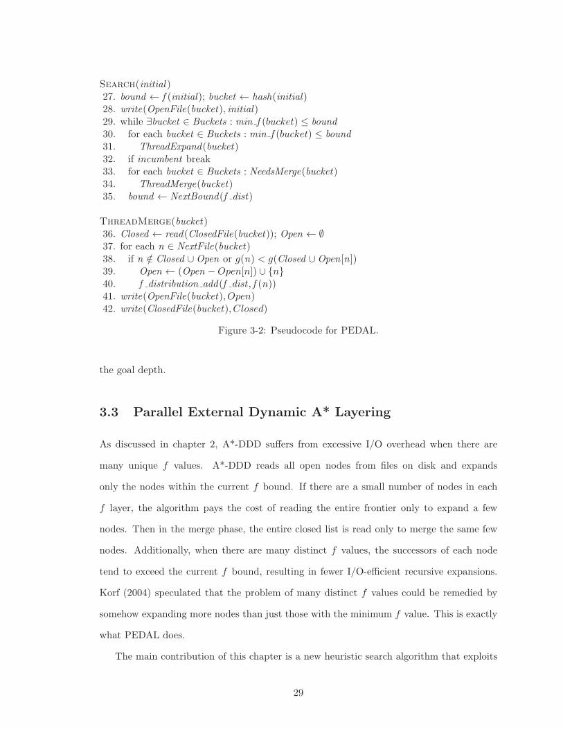
Search(initial)27. bound ← f (initial); bucket ← hash(initial)28. write(OpenFile(bucket), initial)29. while ∃bucket ∈ Buckets : min f (bucket) ≤ bound30. for each bucket ∈ Buckets : min f (bucket) ≤ bound31. ThreadExpand(bucket)32. if incumbent break33. for each bucket ∈ Buckets : NeedsMerge(bucket)34. ThreadMerge(bucket)35. bound ← NextBound(f dist)

ThreadMerge(bucket)36. Closed ← read(ClosedFile(bucket)); Open ← ∅37. for each n ∈ NextFile(bucket)38. if n /∈ Closed ∪Open or g(n) < g(Closed ∪Open[n])39. Open ← (Open −Open[n]) ∪ {n}40. f distribution add(f dist , f (n))41. write(OpenFile(bucket), Open)42. write(ClosedFile(bucket), Closed)

Figure 3-2: Pseudocode for PEDAL.

the goal depth.

3.3 Parallel External Dynamic A* Layering

As discussed in chapter 2, A*-DDD suffers from excessive I/O overhead when there are

many unique f values. A*-DDD reads all open nodes from files on disk and expands

only the nodes within the current f bound. If there are a small number of nodes in each

f layer, the algorithm pays the cost of reading the entire frontier only to expand a few

nodes. Then in the merge phase, the entire closed list is read only to merge the same few

nodes. Additionally, when there are many distinct f values, the successors of each node

tend to exceed the current f bound, resulting in fewer I/O-efficient recursive expansions.

Korf (2004) speculated that the problem of many distinct f values could be remedied by

somehow expanding more nodes than just those with the minimum f value. This is exactly

what PEDAL does.

The main contribution of this chapter is a new heuristic search algorithm that exploits

29

external memory and parallelism and can handle arbitrary f cost distributions. It can be

seen as a combination of A*-DDD and the estimation technique inspired by IDA*CR to

dynamically layer the search space. We call the algorithm Parallel External search with

Dynamic A* Layering (PEDAL).

Like HBDDD-A*, PEDAL proceeds in two phases: an expansion phase and a merge

phase. However, during the merge phase, it tracks the distribution of the f values of

the frontier nodes that were determined not to be duplicates. This distribution is used

to select the f bound for the next expansion phase that will give a constant number of

expansions per node I/O. The pseudo-code for PEDAL, given in Figure 3-2, is adapted

from the pseudo-code for A*-DDD given in Figure 2-1. The main difference is at lines 35

and 40 where PEDAL records the f value of all nodes that are added to the frontier and

uses this distribution to select the next bound for the following expansion phase. Another

critical difference is that, since PEDAL relaxes the best-first search order, it must perform

branch-and-bound after an incumbent solution is found.

3.3.1 Overhead

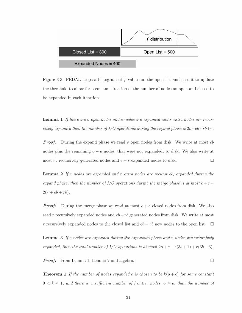
PEDAL uses a technique inspired by IDA*CR to maintain a bound schedule such that the

number of nodes expanded is at least a constant fraction of the amount of I/O at each

iteration. We keep a histogram of f values for all nodes on the open list and a count of the

total number of nodes on the closed list. The next bound is selected to be a constant fraction

of the sum of nodes on the open and closed lists. Unlike IDA*CR which only provides a

heuristic for the desired doubling behavior, the technique used by PEDAL is guaranteed to

give only bounded I/O overhead.

We now confirm that this simple scheme ensures constant I/O overhead, that is, the

number of nodes expanded is at least a constant fraction of the number of nodes read from

and written to disk. We assume a constant branching factor b and that the number of

frontier nodes remaining after duplicate detection is always large enough to expand the

desired number of nodes. We begin with a few useful lemmata.

30

Closed List = 300 Open List = 500

Expanded Nodes = 400

f distribution

Figure 3-3: PEDAL keeps a histogram of f values on the open list and uses it to update

the threshold to allow for a constant fraction of the number of nodes on open and closed to

be expanded in each iteration.

Lemma 1 If there are o open nodes and e nodes are expanded and r extra nodes are recur-

sively expanded then the number of I/O operations during the expand phase is 2o+eb+rb+r.

Proof: During the expand phase we read o open nodes from disk. We write at most eb

nodes plus the remaining o − e nodes, that were not expanded, to disk. We also write at

most rb recursively generated nodes and e+ r expanded nodes to disk. �

Lemma 2 If e nodes are expanded and r extra nodes are recursively expanded during the

expand phase, then the number of I/O operations during the merge phase is at most c+ e+

2(r + eb+ rb).

Proof: During the merge phase we read at most c + e closed nodes from disk. We also

read r recursively expanded nodes and eb+rb generated nodes from disk. We write at most

r recursively expanded nodes to the closed list and eb+ rb new nodes to the open list. �

Lemma 3 If e nodes are expanded during the expansion phase and r nodes are recursively

expanded, then the total number of I/O operations is at most 2o+ c+ e(3b+1)+ r(3b+3).

Proof: From Lemma 1, Lemma 2 and algebra. �

Theorem 1 If the number of nodes expanded e is chosen to be k(o+ c) for some constant

0 < k ≤ 1, and there is a sufficient number of frontier nodes, o ≥ e, than the number of

31

nodes expanded is bounded by a constant fraction of the total number of I/O operations for

some constant q.

Proof:

total I /O

= e(3b+ 1) + r(3b+ 3) + 2o+ c by Lemma 3

< e(3b+ 3) + r(3b+ 3) + 2o+ c

= ze+ zr + 2o+ c for z = (3b+ 3)

= zko+ zkc+ zr + 2o+ c for e = ko+ kc

= o(zk + 2) + c(zk + 1) + zr

< o(zk + 2) + c(zk + 2) + zr

< qko+ qkc+ qr for q ≥ (zk + 2)/k

= q(ko+ kc+ r)

= q(e+ r) because e = k(o+ c)

= q · total expanded

Because q ≥ (zk + 2)/k = (3b+ 3) + 2/k is constant, the theorem holds. �

3.3.2 Empirical Evaluation

We evaluated the performance of PEDAL on two domains with a wide range of edge costs:

the square root sliding-tile puzzle and a dock robot planning domain. For these experiments,

we implemented a novel variant of BFHS-DDD that uses the IDA*CR technique for setting

the upper bound at each iteration. As in the previous experiments, our implementation of

BFHS-DDD does not perform solution reconstruction and therefore the results presented

give a lower bound on its actual solution times.

The Square Root 15-Puzzle

The sliding-tile puzzle is one of the most famous heuristic search domains because it is

simple to encode and the actual physical puzzle has fascinated people for many years. This

domain, however, lacks an important feature that many real-world applications of heuristic

32

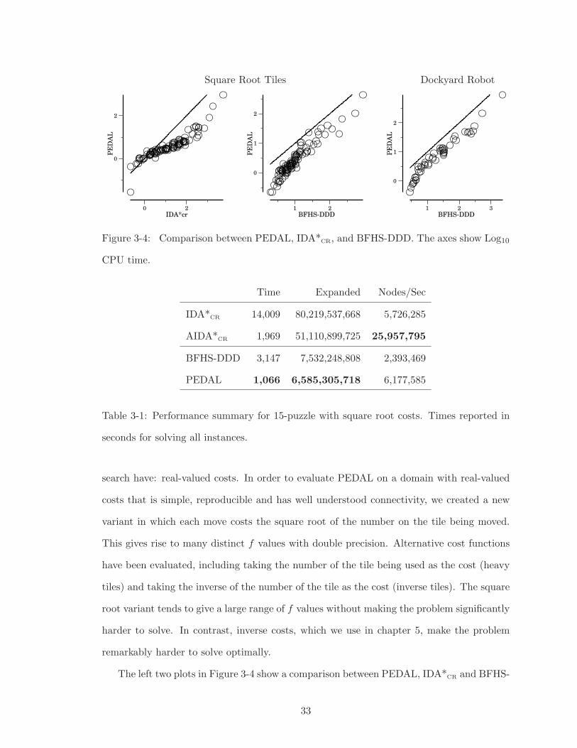
Square Root Tiles Dockyard Robot

IDA*cr

20

PEDAL

2

0

BFHS-DDD

21

PEDAL

2

1

0

BFHS-DDD

321

PEDAL

2

1

0

Figure 3-4: Comparison between PEDAL, IDA*CR, and BFHS-DDD. The axes show Log10

CPU time.

Time Expanded Nodes/Sec

IDA*CR 14,009 80,219,537,668 5,726,285

AIDA*CR 1,969 51,110,899,725 25,957,795

BFHS-DDD 3,147 7,532,248,808 2,393,469

PEDAL 1,066 6,585,305,718 6,177,585

Table 3-1: Performance summary for 15-puzzle with square root costs. Times reported in

seconds for solving all instances.

search have: real-valued costs. In order to evaluate PEDAL on a domain with real-valued

costs that is simple, reproducible and has well understood connectivity, we created a new

variant in which each move costs the square root of the number on the tile being moved.

This gives rise to many distinct f values with double precision. Alternative cost functions

have been evaluated, including taking the number of the tile being used as the cost (heavy

tiles) and taking the inverse of the number of the tile as the cost (inverse tiles). The square

root variant tends to give a large range of f values without making the problem significantly

harder to solve. In contrast, inverse costs, which we use in chapter 5, make the problem

remarkably harder to solve optimally.

The left two plots in Figure 3-4 show a comparison between PEDAL, IDA*CR and BFHS-

33

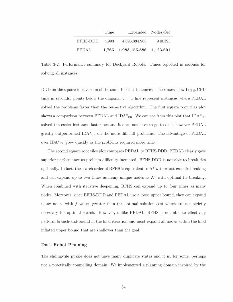
Time Expanded Nodes/Sec

BFHS-DDD 4,993 4,695,394,966 940,395

PEDAL 1,765 1,983,155,888 1,123,601

Table 3-2: Performance summary for Dockyard Robots. Times reported in seconds for

solving all instances.

DDD on the square root version of the same 100 tiles instances. The x axes show Log10 CPU

time in seconds: points below the diagonal y = x line represent instances where PEDAL

solved the problems faster than the respective algorithm. The first square root tiles plot

shows a comparison between PEDAL and IDA*CR. We can see from this plot that IDA*CR

solved the easier instances faster because it does not have to go to disk, however PEDAL

greatly outperformed IDA*CR on the more difficult problems. The advantage of PEDAL

over IDA*CR grew quickly as the problems required more time.

The second square root tiles plot compares PEDAL to BFHS-DDD. PEDAL clearly gave

superior performance as problem difficulty increased. BFHS-DDD is not able to break ties

optimally. In fact, the search order of BFHS is equivalent to A* with worst-case tie breaking

and can expand up to two times as many unique nodes as A* with optimal tie breaking.

When combined with iterative deepening, BFHS can expand up to four times as many

nodes. Moreover, since BFHS-DDD and PEDAL use a loose upper bound, they can expand

many nodes with f values greater than the optimal solution cost which are not strictly

necessary for optimal search. However, unlike PEDAL, BFHS is not able to effectively

perform branch-and-bound in the final iteration and must expand all nodes within the final

inflated upper bound that are shallower than the goal.

Dock Robot Planning

The sliding-tile puzzle does not have many duplicate states and it is, for some, perhaps

not a practically compelling domain. We implemented a planning domain inspired by the

34

dockyard robot example used throughout the textbook by Ghallab, Nau, and Traverso

(2004). In the dockyard robot domain, which is NP-hard, containers must be moved from

their initial locations to their desired destinations via a robot that can carry only a single

container at a time. The containers at each location form a stack from which the robot can

only access the top container by using a crane that resides at the given location. Accessing

a container that is not at the top of a stack therefore requires moving the upper container

to a stack at a different location. The available actions are: load a container from a crane

into the robot, unload a container from the robot into a crane, take the top container from

the pile using a crane, put the container in the crane onto the top of a pile and move the

robot between adjacent locations.

The load and unload actions have a constant cost of 0.01, accessing a pile with a crane

costs 0.05 times the height of the pile plus 1 (to ensure non-zero-cost actions) and movement

between locations costs the distance between locations. For these experiments, the location

graph was created by placing random points on a unit square. The length of each edge

was the Euclidean distance between the end points. The heuristic lower bound sums the

distance of each container’s current location from its goal location. We conducted these

experiments on a configuration with 5 locations, cranes, piles and 8 containers. We used a

total of 50 instances and selected a hash function that maps states to buckets by ignoring

all except the position of the robot and three containers.

Moreover, because of the large number of duplicate states IDA*CR failed to solve all

instances within the time limit so we do not show results for it. PEDAL and BFHS-DDD

were able to solve all instances. The right-most plot in Figure 3-4 shows a comparison

between PEDAL and BFHS-DDD. Again, points below the diagonal represent instances

where PEDAL had the faster solution time. We can see from the plot that all of the points

lie below the y = x line and therefore PEDAL outperformed BFHS-DDD on every instance.

These results provide evidence to suggest that a best-first search order is competitive

in an external memory setting. It significantly reduces the number of nodes generated

which corresponds to many fewer expensive I/O operations. BFHS uses a breadth-first

35

search strategy to reduce the space complexity by removing the closed list. However, the

performance bottleneck for the search problems examined in this chapter is the rapidly

growing search frontier, not the closed list. Thus, the breadth-first search order of BFHS

provides no advantage.

3.4 Conclusion

In this chapter we presented a new parallel external-memory search with dynamic A* lay-

ering (PEDAL) that combines ideas from A*-DDD and IDA*CR. We proved that a simple

layering scheme allows PEDAL to guarantee a constant I/O overhead. In addition, we

showed empirically that PEDAL gives very good performance in practice, solving a real-cost

variant of the sliding-tile puzzle more quickly than both IDA*CR and BFHS and it surpasses

BFHS on the more practically motivated dockyard robot domain. PEDAL demonstrates

that best-first heuristic search can scale to large problems that have real costs. In the

next chapter we show how PEDAL can be extended to scale to problems that have large

branching factors and achieve a new state-of-the-art for the problem of Multiple Sequence

Alignment.

36

CHAPTER 4

EXTERNAL MEMORY SEARCH WITH

LARGE BRANCHING FACTORS

4.1 Introduction

One real-world application of heuristic search with practical relevance (Korf, 2012) is Multi-

ple Sequence Alignment (MSA). MSA can be formulated as a shortest path problem where

each sequence represents one dimension in a multi-dimensional lattice and a solution is a

least-cost path through the lattice. To achieve biologically plausible alignments, great care

must be taken in selecting the most relevant cost function. The scoring of gaps is of par-

ticular importance. Altschul (1989) recommends affine gap costs, described in more detail

below, which increase the size of the state space by a factor of 2k for k sequences. Due to

the large branching factor of 2k − 1, the performance bottleneck for MSA is the memory

required to store the frontier of the search.

Although dynamic programming is the classic technique for solving MSA (Needleman &

Wunsch, 1970), heuristic search algorithms can achieve better performance than dynamic

programming by pruning much of the search space, computing alignments faster and using

less memory (Ikeda & Imai, 1999). A* (Hart et al., 1968) uses an admissible heuristic

function to avoid exploring much of the search space. The classic A* algorithm maintains an

open list, containing nodes that have been generated but not yet expanded, and a closed list,

containing all generated states, in order to prevent duplicated search effort. Unfortunately,

for challenging MSA problems, the memory required to maintain the open and closed lists

makes A* impractical.

Yoshizumi, Miura, and Ishida (2000) present a variant of A* called Partial Expansion

37

A* (PEA*) that reduces the memory needed to store the open list by storing only the

successor nodes that appear promising. This technique can significantly reduce the size of

the open list. However, like A*, PEA* is limited by the memory required to store the open

and closed list and for challenging alignment problems PEA* can still exhaust memory.

One previously proposed alternative to PEA* is Iterative Deepening Dynamic Program-

ming (IDDP, Schroedl, 2005), a form of bounded dynamic programming that relies on an

uninformed search order to reduce the maximum number of nodes that need to be stored

during search. The memory savings of IDDP comes at the cost of repeated search effort and

divide-and-conquer solution reconstruction. IDDP forgoes a best-first search order and as

a result it is possible for IDDP to visit many more nodes than a version of A* with optimal

tie-breaking. Moreover, because of the wide range of edge costs found in the MSA domain,

IDDP must rely on the bound setting technique of IDA*CR (Sarkar et al., 1991). With this

technique, it is possible for IDDP to visit four times as many nodes as A* (Schroedl, 2005).

And even though IDDP reduces the size of the frontier, it is still limited by the amount

of memory required to store the open nodes and for large MSA problems this can exhaust

main memory.

Rather than suffer the overhead of an uninformed search order and divide-and-conquer

solution reconstruction, we propose, as in the previous chapter, solving large problems by

combining best-first search with external memory search. In this chapter we present a new

general-purpose algorithm Parallel External Partial Expansion A* (PE2A*), that combines

the best-first partial expansion technique of PEA* and the external memory technique of

HBDDD. We compare PE2A* with in-memory A*, PEA* and IDDP for solving challenging

instances of MSA. The results show that parallel external memory best-first search can

outperform serial in-memory search and is capable of solving large problems that cannot fit

in main memory. Contrary to the assumptions of previous work, we find that storing the

open list is much more expensive than storing the closed list. We also demonstrate that

PE2A* is capable of solving, for the first time, the entire Reference Set 1 of the BAliBASE

benchmark for MSA (Thompson, Plewniak, & Poch, 1999) using a biologically plausible

38

A C T G _Alignment:

A C T G

C

T

G

G

_ C T G G

Score Matrix:

A C T G

A

C

T

G

0 4 2 2

1 4 3

0 6

1

_

3

3

3

3

_ 0

3+1+0+1+3 = 8Cost:

Figure 4-1: Optimal sequence alignment using a lattice and scoring matrix.

cost function that incorporates affine gap costs. This work suggests that external best-first

search can effectively use heuristic information to surpass methods that rely on uninformed

search orders.

4.2 Multiple Sequence Alignment

We first discuss the MSA problem in more detail, including computing heuristic estimates.

Then we will review the most popular applicable heuristic search algorithms.

4.2.1 MSA as a Shortest Path Problem

In Bioinformatics, alignments are computed in order to identify the most similar regions

between two ore more sequences of DNA. An alignment also represents the most likely set

of changes necessary to transform one sequence into the other. One way to compute an

alignment is to find an optimal placement of gaps in each of the sequences that maximizes

the amount of overlapping regions.

In the case of aligning two sequences, an optimal (most plausible) pair–wise alignment

39

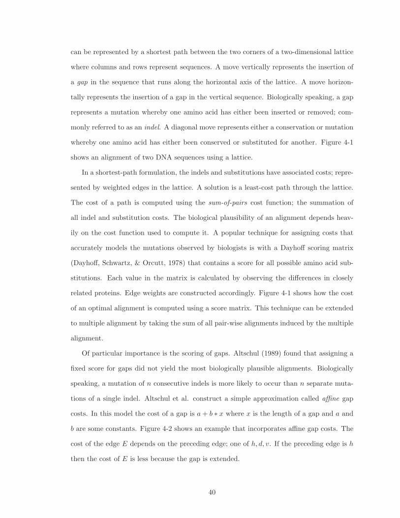
can be represented by a shortest path between the two corners of a two-dimensional lattice

where columns and rows represent sequences. A move vertically represents the insertion of

a gap in the sequence that runs along the horizontal axis of the lattice. A move horizon-

tally represents the insertion of a gap in the vertical sequence. Biologically speaking, a gap

represents a mutation whereby one amino acid has either been inserted or removed; com-

monly referred to as an indel. A diagonal move represents either a conservation or mutation

whereby one amino acid has either been conserved or substituted for another. Figure 4-1

shows an alignment of two DNA sequences using a lattice.

In a shortest-path formulation, the indels and substitutions have associated costs; repre-

sented by weighted edges in the lattice. A solution is a least-cost path through the lattice.

The cost of a path is computed using the sum-of-pairs cost function; the summation of

all indel and substitution costs. The biological plausibility of an alignment depends heav-

ily on the cost function used to compute it. A popular technique for assigning costs that

accurately models the mutations observed by biologists is with a Dayhoff scoring matrix

(Dayhoff, Schwartz, & Orcutt, 1978) that contains a score for all possible amino acid sub-

stitutions. Each value in the matrix is calculated by observing the differences in closely

related proteins. Edge weights are constructed accordingly. Figure 4-1 shows how the cost

of an optimal alignment is computed using a score matrix. This technique can be extended

to multiple alignment by taking the sum of all pair-wise alignments induced by the multiple

alignment.

Of particular importance is the scoring of gaps. Altschul (1989) found that assigning a

fixed score for gaps did not yield the most biologically plausible alignments. Biologically

speaking, a mutation of n consecutive indels is more likely to occur than n separate muta-

tions of a single indel. Altschul et al. construct a simple approximation called affine gap

costs. In this model the cost of a gap is a+ b ∗ x where x is the length of a gap and a and

b are some constants. Figure 4-2 shows an example that incorporates affine gap costs. The

cost of the edge E depends on the preceding edge; one of h, d, v. If the preceding edge is h

then the cost of E is less because the gap is extended.

40

d

h

v

E

E(v) = 8 + 3

E(d) = 8 + 3

E(h) = 3

Gap Cost: = 3Gap Penalty: = 8

Figure 4-2: Computing edge costs with affine gaps. The cost of edge E depends on the

incoming edge; one of h, d or v. If the incoming edge is v or d, then E represents the start

of a gap, and incurs a gap start penalty of 8. However, if the incoming edge is h then E

represents the continuation of a gap and incurs no gap start penalty.

A pair-wise alignment is easily computed using dynamic programming (Needleman &

Wunsch, 1970). This method could be extended to alignments of k sequences in the form

of a k dimensional lattice. However, for alignments of higher dimensions, the Nk time and

space required render dynamic programming infeasible. This motivates the use of heuristic

search algorithms that are capable of finding an optimal solution while pruning much of

the search space with the help of an admissible heuristic. While affine gap costs have been

shown to improve accuracy, they also increase the size of the state space. This is because

each state is uniquely identified not only by the lattice coordinates but also by the incoming

edge; indicating whether a gap has been started. This increases the state space by a factor

of 2k for aligning k sequences. Affine gap costs also make the MSA domain implementation

more complex and require more memory for storing the heuristic.

4.2.2 Admissible Heuristics

The cost of a k-fold optimal alignment is computed by taking the sum of all pair-wise

alignments using the same pair-wise cost function above. Carrillo and Lipman (1988) show

that the cost of an optimal alignment for k sequences is greater than or equal to the sum of

all possible m-fold optimal alignments of the same sequences for m ≤ k. Therefore, we can

construct a lower bound on the cost of an optimal alignment of k sequences by taking the

41

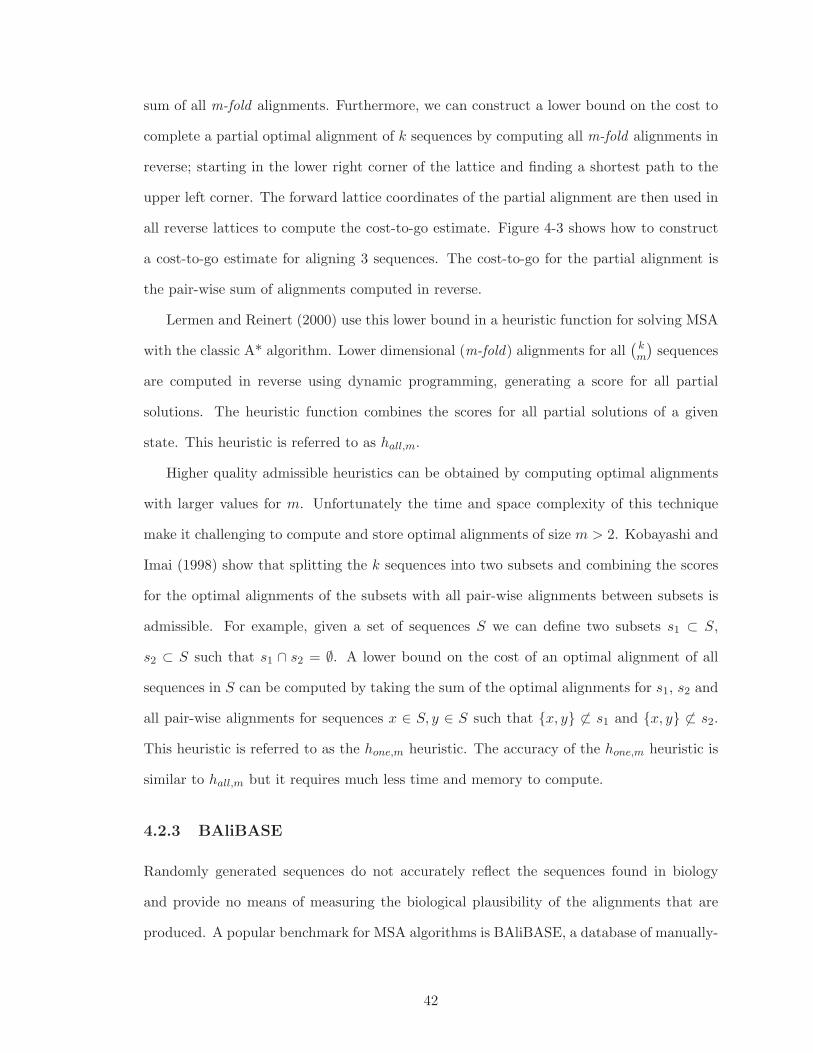
sum of all m-fold alignments. Furthermore, we can construct a lower bound on the cost to

complete a partial optimal alignment of k sequences by computing all m-fold alignments in

reverse; starting in the lower right corner of the lattice and finding a shortest path to the

upper left corner. The forward lattice coordinates of the partial alignment are then used in

all reverse lattices to compute the cost-to-go estimate. Figure 4-3 shows how to construct

a cost-to-go estimate for aligning 3 sequences. The cost-to-go for the partial alignment is

the pair-wise sum of alignments computed in reverse.

Lermen and Reinert (2000) use this lower bound in a heuristic function for solving MSA

with the classic A* algorithm. Lower dimensional (m-fold) alignments for all(km

)sequences

are computed in reverse using dynamic programming, generating a score for all partial

solutions. The heuristic function combines the scores for all partial solutions of a given

state. This heuristic is referred to as hall,m.

Higher quality admissible heuristics can be obtained by computing optimal alignments

with larger values for m. Unfortunately the time and space complexity of this technique

make it challenging to compute and store optimal alignments of size m > 2. Kobayashi and

Imai (1998) show that splitting the k sequences into two subsets and combining the scores

for the optimal alignments of the subsets with all pair-wise alignments between subsets is

admissible. For example, given a set of sequences S we can define two subsets s1 ⊂ S,

s2 ⊂ S such that s1 ∩ s2 = ∅. A lower bound on the cost of an optimal alignment of all

sequences in S can be computed by taking the sum of the optimal alignments for s1, s2 and

all pair-wise alignments for sequences x ∈ S, y ∈ S such that {x, y} 6⊂ s1 and {x, y} 6⊂ s2.

This heuristic is referred to as the hone,m heuristic. The accuracy of the hone,m heuristic is

similar to hall,m but it requires much less time and memory to compute.

4.2.3 BAliBASE

Randomly generated sequences do not accurately reflect the sequences found in biology

and provide no means of measuring the biological plausibility of the alignments that are

produced. A popular benchmark for MSA algorithms is BAliBASE, a database of manually-

42

A C T

C

T

G

A C T

C

T

T

C T G

C

T

T

cost to gopartial alignment

A C T _

_ C T G_ C T T

6 + 3 0 + 12

Seq 1 Seq 1

Seq 2Seq 2

Seq 3

Seq 3

Figure 4-3: Computing cost-to-go by solving the lattice in reverse.

refined multiple sequence alignments specifically designed for the evaluation and comparison

of multiple sequence alignment programs (Thompson et al., 1999). Of particular interest to

our study is a set of instances known as Reference Set 1. Each instance in this set contains

4 to 6 protein sequences that range in length from 58 to 993. The sequences in this set

are challenging for optimal MSA programs because they are highly dissimilar; requiring

that much of the state space be explored to find an optimal alignment. To the best of our

knowledge, no one has been able to compute optimal alignments for the entire Reference

Set 1 using affine gap costs.

4.3 Previous Work

4.3.1 Iterative-Deepening Dynamic Programming

Iterative Deepening Dynamic-Programming (IDDP, (Schroedl, 2005)) is an iterative deep-

ening search that combines dynamic programming with an admissible heuristic for pruning.

43

IDDP uses a pre-defined search order much like dynamic programming. The state space is

divided into levels that can be defined row-wise, column-wise or by antidiagonals (lower-

left to upper-right). IDDP proceeds by expanding nodes one level at a time. To detect

duplicates, only the adjacent levels are needed. All other previously expanded levels may

be deleted. This pre-defined expansion order reduces the amount of memory required to

store open nodes: if levels are defined by antidiagonals then only k levels need to be stored

in the open list during search, where k is the number of sequences being aligned. In this

case the maximum size of the open list is O(kNk−1) for sequences of length N . This is one

dimension smaller than the entire space O(Nk).

IDDP uses a heuristic function, similar to A*, to prune unpromising nodes and in

practice the size of the open list is much smaller than the worst case. At each iteration of

the search an upper bound b on the solution cost is estimated and only the nodes with f ≤ b

are expanded. IDDP uses the same bound setting technique of IDA*CR (Sarkar et al., 1991)

to estimate an upper bound that is expected to double the number of nodes expanded at

each iteration.

Schroedl (2005) was able to compute optimal alignments for 80 of the 82 instances

in Reference Set 1 of the BAliBASE benchmark using IDDP with a cost function that

incorporated affine gap costs. Edelkamp and Kissmann (2007) extend IDDP to external

memory search using sorting-based DDD but were only able to solve one additional instance,

gal4 which alone required over 182 hours of solving time.

Because IDDP deletes closed nodes, divide-and-conquer solution reconstruction is re-

quired to recover the solution. As we will see later, deleting closed nodes provides a limited

advantage since the size of the closed list is just a small fraction of the number of nodes

generated during search.

In order to achieve memory savings, IDDP expands nodes in an uninformed pre-defined

expansion order. In contrast to a best-first expansion order, a node in one level may be

expanded before a node in another level with a lower f . As a result, it is possible for

IDDP to expand many more nodes in the final f layer than A* with optimal tie-breaking.

44

In fact, the expansion order of IDDP approximates worst-case tie-breaking. The preferred

tie-breaking policy for A* is to break ties by expanding nodes with higher g first. The g

of a goal node is maximal among all nodes with equal f . Therefore, as soon as the goal

node is generated it is placed at the front of the open list and search can terminate on the

next expansion. In contrast, IDDP will expand all non-goal nodes n with f(n) ≤ C∗ where

C∗ is the cost of an optimal solution. This is because in the final iteration the bound is

set to b ≥ C∗ and all nodes n with f(n) ≤ C∗ ≤ b are expanded at each level. The level

containing the goal is processed last and therefore all non-goal nodes n with f(n) ≤ C∗

must be expanded first.

The situation is even worse when relying on the bound setting technique of IDA*CR.

This technique estimates each bound in an attempt to double the number of expanded

nodes at each iteration. Since the search order of IDDP is not best-first, it must visit all

nodes in the final iteration to ensure optimality, which can include many nodes with f > C∗.

If doubling is achieved, then it is possible for IDDP to visit four times as many nodes as

A* (Schroedl, 2005).

4.3.2 Partial Expansion A*

When expanding a node, search algorithms typically generate and store all successor nodes,

many of which have an f that is greater than the optimal solution cost. These nodes take

up space on the open list, yet are never expanded. PEA* (Yoshizumi et al., 2000) reduces

the memory needed to store the open list by pruning the successor nodes that do not appear

promising i.e., nodes that are not likely to be expanded. A node appears promising if its f

does not exceed the f of its parent node plus some constant C. Partially expanded nodes

are put back on the open list with a new f equal to the minimum f of the successor nodes

that were pruned. We designate the updated f values as F (n).

Yoshizumi et al. (2000) show that for MSA, PEA* is able to reduce the memory require-

ment of the classic A* algorithm by a factor of 100. The reduced memory comes at the cost

of having to repeatedly expand partially expanded nodes until all of their successors have

45

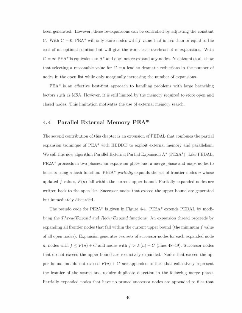
been generated. However, these re-expansions can be controlled by adjusting the constant

C. With C = 0, PEA* will only store nodes with f value that is less than or equal to the

cost of an optimal solution but will give the worst case overhead of re-expansions. With

C =∞ PEA* is equivalent to A* and does not re-expand any nodes. Yoshizumi et al. show

that selecting a reasonable value for C can lead to dramatic reductions in the number of

nodes in the open list while only marginally increasing the number of expansions.

PEA* is an effective best-first approach to handling problems with large branching

factors such as MSA. However, it is still limited by the memory required to store open and

closed nodes. This limitation motivates the use of external memory search.

4.4 Parallel External Memory PEA*

The second contribution of this chapter is an extension of PEDAL that combines the partial

expansion technique of PEA* with HBDDD to exploit external memory and parallelism.

We call this new algorithm Parallel External Partial Expansion A* (PE2A*). Like PEDAL,

PE2A* proceeds in two phases: an expansion phase and a merge phase and maps nodes to

buckets using a hash function. PE2A* partially expands the set of frontier nodes n whose

updated f values, F (n) fall within the current upper bound. Partially expanded nodes are

written back to the open list. Successor nodes that exceed the upper bound are generated

but immediately discarded.

The pseudo code for PE2A* is given in Figure 4-4. PE2A* extends PEDAL by modi-

fying the ThreadExpand and RecurExpand functions. An expansion thread proceeds by

expanding all frontier nodes that fall within the current upper bound (the minimum f value

of all open nodes). Expansion generates two sets of successor nodes for each expanded node

n; nodes with f ≤ F (n) + C and nodes with f > F (n) + C (lines 48–49). Successor nodes

that do not exceed the upper bound are recursively expanded. Nodes that exceed the up-

per bound but do not exceed F (n) + C are appended to files that collectively represent

the frontier of the search and require duplicate detection in the following merge phase.

Partially expanded nodes that have no pruned successor nodes are appended to files that

46

ThreadExpand(bucket)43. for each state ∈ Read(OpenFile(bucket))44. if F (state) ≤ bound45. RecurExpand(state)46. else append(NextFile(bucket), state)

RecurExpand(n)47. if IsGoal(n) incumbent ← n; return48. SUCCp ← {np |np ∈ succ(n), f (np) ≤ F (n) + C}49. SUCCq ← {nq |nq ∈ succ(n), f (nq) > F (n) + C}50. for each succ ∈ SUCCp

51. if f (succ) ≤ bound52. RecurExpand(succ)53. else54. append(NextFile(hash(succ)), succ)55. if SUCCq = ∅56. append(ClosedFile(hash(n)),n)57. else58. F (n)← min f (nq),nq ∈ SUCCq

59. append(NextFile(hash(n)),n)

Figure 4-4: Pseudocode for the PE2A* algorithm.

collectively represent the closed list (lines 55–56). Partially expanded nodes with pruned

successor nodes are updated with a new F and appended to the frontier (lines 58–59).

PE2A* approximates optimal tie-breaking by sorting buckets according to the minimum F

of all nodes in each bucket.

4.5 Empirical Evaluation

To determine the effectiveness of this approach, we compared A*, PEA*, IDDP, A*-DDD

and PE2A* on the problem of multiple sequence alignment using the PAM 250 Dayhoff

substitution matrix with affine gap costs. All experiments were run on Machine-B, a dual

hexa-core machine (12 cores) with Xeon X5660 2.80 GHz processors, 12 GB of RAM and

12 320 GB disks. The files generated by the external memory search algorithms were

distributed uniformly among all 12 disks to enable parallel I/O. We found that using a

47

number of threads that is equal to the number of disks gave best performance. We tried a

range of values for C from 0 to 500 and found that 100 performed best.

One advantage of an uninformed search order is that the open list does not need to

be sorted. IDDP was implemented using an open list that consisted of an array of linked

lists. We found IDDP to be sensitive to the number of bins used when estimating the

next bound; 500 bins performed well. We stored all closed nodes in a hash table and to

improve time performance did not implement the SparsifyClosed procedure (a procedure

that removes unneeded nodes from the closed list) as described by Schroedl (2005). Since we

did not remove any closed nodes we did not have to implement divide-and-conquer solution

reconstruction.

We used the pair-wise (hall,2) heuristic to solve 80 of the 82 instances in the BAliBASE

Reference Set 1 benchmark. This was primarily because the memory required to store the

hall,3 heuristic exceeded the amount of memory available. For example, instance 1taq has

a maximum sequence length of 929. To store just one 3-fold alignment using affine gap

costs, we would need to store 9293 × 7× 4 bytes or approximately 21 GB, assuming 32-bit

integers. The maximum sequence length for the hardest 2 instances is 573, allowing us to

fit the hone,3 heuristic. For the 75 easiest instances, we used a hash function that used the

lattice coordinate of the longest sequence. For all other instances we used a hash function

that used the lattice coordinates of the two longest sequences.

Table 4-1 shows results for solving the 75 easiest instances of BAliBASE Reference Set

1. In the first set of rows we see that IDDP expands 1.7 times more nodes than PEA*

and nearly 3 times more nodes than A*. The total solving time for IDDP is approximately

1.6 times longer than A* and PEA*. These results are consistent with results reported by

Schroedl (2005) for alignments consisting of 6 or fewer sequences. We also see that the

partial expansion technique is effective in reducing the number of nodes generated by a

factor of 5. IDDP generates 1.96 times more nodes than PEA*.

In all instances, A* generates and stores many more nodes than it expands. For example,

for instance 1sbp A* generates approximately 64,230,344 unique nodes while expanding only

48

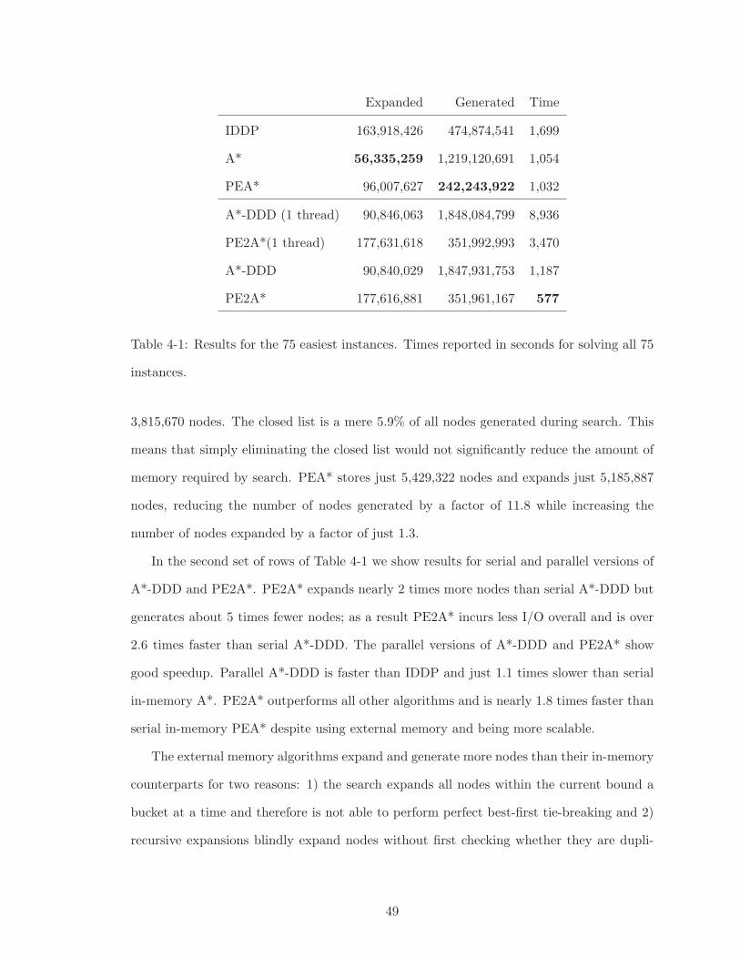
Expanded Generated Time

IDDP 163,918,426 474,874,541 1,699

A* 56,335,259 1,219,120,691 1,054

PEA* 96,007,627 242,243,922 1,032

A*-DDD (1 thread) 90,846,063 1,848,084,799 8,936

PE2A*(1 thread) 177,631,618 351,992,993 3,470

A*-DDD 90,840,029 1,847,931,753 1,187

PE2A* 177,616,881 351,961,167 577

Table 4-1: Results for the 75 easiest instances. Times reported in seconds for solving all 75

instances.

3,815,670 nodes. The closed list is a mere 5.9% of all nodes generated during search. This

means that simply eliminating the closed list would not significantly reduce the amount of

memory required by search. PEA* stores just 5,429,322 nodes and expands just 5,185,887

nodes, reducing the number of nodes generated by a factor of 11.8 while increasing the

number of nodes expanded by a factor of just 1.3.

In the second set of rows of Table 4-1 we show results for serial and parallel versions of

A*-DDD and PE2A*. PE2A* expands nearly 2 times more nodes than serial A*-DDD but

generates about 5 times fewer nodes; as a result PE2A* incurs less I/O overall and is over

2.6 times faster than serial A*-DDD. The parallel versions of A*-DDD and PE2A* show

good speedup. Parallel A*-DDD is faster than IDDP and just 1.1 times slower than serial

in-memory A*. PE2A* outperforms all other algorithms and is nearly 1.8 times faster than

serial in-memory PEA* despite using external memory and being more scalable.

The external memory algorithms expand and generate more nodes than their in-memory

counterparts for two reasons: 1) the search expands all nodes within the current bound a

bucket at a time and therefore is not able to perform perfect best-first tie-breaking and 2)

recursive expansions blindly expand nodes without first checking whether they are dupli-

49

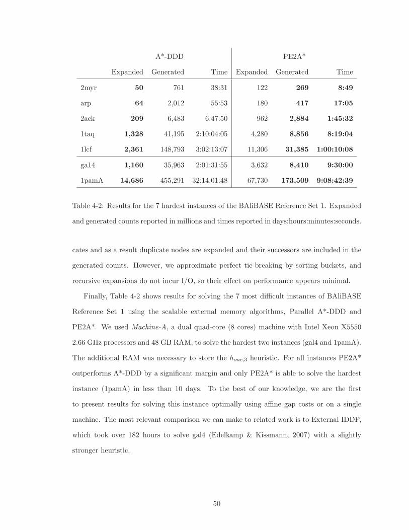
A*-DDD PE2A*

Expanded Generated Time Expanded Generated Time

2myr 50 761 38:31 122 269 8:49

arp 64 2,012 55:53 180 417 17:05

2ack 209 6,483 6:47:50 962 2,884 1:45:32

1taq 1,328 41,195 2:10:04:05 4,280 8,856 8:19:04

1lcf 2,361 148,793 3:02:13:07 11,306 31,385 1:00:10:08

ga14 1,160 35,963 2:01:31:55 3,632 8,410 9:30:00

1pamA 14,686 455,291 32:14:01:48 67,730 173,509 9:08:42:39

Table 4-2: Results for the 7 hardest instances of the BAliBASE Reference Set 1. Expanded

and generated counts reported in millions and times reported in days:hours:minutes:seconds.

cates and as a result duplicate nodes are expanded and their successors are included in the

generated counts. However, we approximate perfect tie-breaking by sorting buckets, and

recursive expansions do not incur I/O, so their effect on performance appears minimal.

Finally, Table 4-2 shows results for solving the 7 most difficult instances of BAliBASE

Reference Set 1 using the scalable external memory algorithms, Parallel A*-DDD and

PE2A*. We used Machine-A, a dual quad-core (8 cores) machine with Intel Xeon X5550

2.66 GHz processors and 48 GB RAM, to solve the hardest two instances (gal4 and 1pamA).

The additional RAM was necessary to store the hone,3 heuristic. For all instances PE2A*

outperforms A*-DDD by a significant margin and only PE2A* is able to solve the hardest

instance (1pamA) in less than 10 days. To the best of our knowledge, we are the first

to present results for solving this instance optimally using affine gap costs or on a single

machine. The most relevant comparison we can make to related work is to External IDDP,

which took over 182 hours to solve gal4 (Edelkamp & Kissmann, 2007) with a slightly

stronger heuristic.

50

4.6 Discussion

We have explored best-first heuristic search in a parallel external memory setting. The

results presented in previous sections provide evidence that maintaining a best-first search

order is beneficial. Alternative algorithms attempt to improve performance by omitting

the closed list with techniques such as a predefined search order. However, for problems

like MSA, the performance bottleneck is the rapidly growing frontier, not the closed list.

While IDDP and BFHS avoid costly I/O by using the previous depth layer for duplicate

checking, this savings is minimal compared to the savings afforded by a best-first search

order, as with PEDAL and PE2A*. A predefined search order results in many more node

expansions than best-first search. Moreover, divide-and-conquer solution reconstruction is

required when omitting the closed list, contributing overhead and complexity to the search.

Algorithms that use an upper bound such as IDDP and BFHS enjoy the advantage of

not having to generate and store nodes that exceed the upper bound. This can avoid costly

I/O for an entire frontier layer. However, the use of such an upper bound often requires

iterative-deepening search which can increase search effort and I/O overhead by a constant

factor. With a best-first search order and optimal tie breaking, the goal node is often

expanded before many of the nodes in the final frontier layer are generated. Furthermore,

the partial expansion technique of PE2A* also avoids generating many nodes in this layer,

saving unnecessary and costly I/O. Another advantage of PEDAL is that it enjoys the

benefit of recursive expansions. These expansions do not incur any I/O and allow for much

faster solving times. IDDP and BFHS cannot benefit from recursive expansions. BFHS

with recursive expansions reduces to IDA* search.

The recursive expansion technique of A*-DDD can give poor performance on domains

where there are many paths to the same node with equal or similar cost. Because duplicate

checking is deferred, many duplicate nodes may be generated that need to be stored in

external memory and later accessed to perform merging. This can result in significant I/O

overhead. One way to deal with this is to bound the depth of recursive expansions, and

in effect bound the number of duplicate nodes that can be generated during the expand

51

phase. Another technique, and one demonstrated in section 2.3, is to employ transposition

tables during the expansion phase. Each thread keeps a local and bounded size closed list

in order to avoid generating many duplicate nodes.

If the closed list is large compared to the size of the open list, then techniques like

BFHS and IDDP may provide superior performance. BFHS and IDDP need only the

current and previous depth layers to check duplicates. Structuring the I/O to support this

is straightforward because of the depth-layered scheme of these algorithms.

A*-DDD based algorithms may perform unnecessary I/O if many of the nodes that

are stored in the closed list are not needed for duplicate merging. However, the pruning

technique of Sparse Memory Graph Search (Zhou & Hansen, 2003a) may provide the same

performance benefit for A*-DDD based algorithms. We leave this for future work.

4.7 Other Related Work

In this section we discuss additional related work.

4.7.1 Parallel Frontier Search

Niewiadomski, Amaral, and Holte (2006) combine parallel Frontier A* search with DDD

(PFA*-DDD). A sampling based technique is used to adaptively partition the workload at

run-time. PFA*-DDD was able to solve the two most difficult problems (gal4 and 1pamA)

of the BAliBASE benchmark using a cluster of 32 dual-core machines. However, affine gap

costs were not used, simplifying the problem and allowing for higher-dimensional heuris-

tics to be computed and stored with less memory. The hardest problem required 16 ma-

chines with a total of 56 GB of RAM. In their experiments, only the costs of the align-

ments were computed. Because Frontier Search deletes closed nodes, recovering the actual

alignments requires extending PFA*-DDD with divide-and-conquer solution reconstruction.

Niewiadomski et al. report that the parallelization of the divide-and-conquer strategy with

PFA*-DDD is non-trivial.

52

4.7.2 External A*

External A* (Edelkamp, Jabbar, & Schrdl, 2004) combines A* with sorting-based DDD.

Nodes of the same g and h values are grouped together in a bucket which maps to a file

on external storage. The search proceeds by iteratively expanding layers of buckets for

which the g and h values sum to the minimum f value among the search frontier. Delayed

duplicate detection is performed by appending nodes to their respective buckets and later

sorting and scanning each bucket to eliminate duplicate nodes. In External A*, the g and

h buckets must be expanded in lowest-g-value-first order which, like BFHS, is equivalent

to the A* search order with worst-case tie breaking and can result in many more node

expansions. Moreover, because of the way buckets are organized according to two values, it

is not obvious how to dynamically inflate each bucket to handle real-valued costs.

4.7.3 Sweep A*

Sweep A* (Zhou & Hansen, 2003b) is a space-efficient algorithm for domains that exhibit

a partial order graph structure. IDDP can be viewed as a special case of Sweep A*. Sweep

A* differs slightly from IDDP in that a best-first expansion order is followed within each

level. This helps find the goal sooner in the final level. However, if levels are defined by

antidiagonals in MSA, then the final level contains very few nodes and they are all goals.

Therefore, the effect of sorting at each level is minimal. Zhou and Hansen (2004) combine

Sweep A* with SDD on a subset of the BAliBASE benchmark without affine gap costs. In

our experiments we compared with IDDP as the algorithms are nearly identical and results

provided by Schroedl (2005) and Edelkamp and Kissmann (2007) for IDDP used affine gap

costs and are thus more relevant to our study.

4.7.4 Enhanced Partial Expansion A*

In practice, PEA* generates all successor nodes and discards the nodes that do not appear

promising. In some cases, it is possible to avoid some of the overhead of generating the

unpromising successor nodes. This observation motivates Enhanced PEA* (EPEA*, Felner,

53

Goldenberg, Sharon, Stern, Beja, Sturtevant, Schaeffer, & Holte, 2012). EPEA* is an

enhanced version of PEA* that improves performance by predicting the cost of nodes,

generating only the promising successors. Unfortunately it is not clear how to predict

successor costs in MSA since the cost of an operator cannot be known a priori.

4.8 Conclusion

In this chapter we have presented PE2A*, an extension of PEDAL that combines the partial

expansion technique of PEA* with hash-based delayed duplicate detection to deal with

problems that have large branching factors. We showed empirically that PE2A* performs

very well in practice, solving 80 of the 82 instances of the BAliBASE Reference Set 1

benchmark with the weaker hall,2 heuristic and the hardest two instances using the hone,3

heuristic. In our experiments, PE2A* outperformed serial PEA*, IDDP and parallel A*-

DDD and was the only algorithm capable of solving the most difficult instance in less than

10 days using the more biologically plausible affine gap cost function. These results add

to a growing body of evidence that a best-first search order can be competitive in scaling

heuristic search.

54

CHAPTER 5

BOUNDED SUBOPTIMAL SEARCH

5.1 Introduction

Verifying that a solution to a heuristic search problem is optimal requires expanding every

node whose f value is less than the optimal solution cost. For many problems of practical

interest, there are too many such nodes to allow the search to complete within a reasonable

amount of time (Helmert & Roger, 2008). These concerns have motivated the development

of bounded suboptimal search algorithms. These algorithms trade increased solution cost

in a principled way for significantly reduced solving time and memory. Given a user-defined

suboptimality bound w, they are guaranteed to return a solution of cost C ≤ w · C∗. A

range of bounded suboptimal search algorithms have been proposed, of which the best-

known is Weighted A∗ (WA∗) algorithm (Pohl, 1973). WA∗ is a best-first search using the

f ′(n) = g(n) + w · h(n) evaluation function.

WA∗ returns solutions with bounded suboptimality only when using an admissible cost-

to-go heuristic h(n). There has been much previous work over the past decade demon-

strating that inadmissible but accurate heuristics can be used effectively to guide search

algorithms (Jabbari Arfaee et al., 2011; Samadi et al., 2008). Inadmissible heuristics can

even be learned online (Thayer et al., 2011). Furthermore, recent work has shown that WA∗

can perform very poorly in domains where the costs of the edges are not uniform (Wilt &

Ruml, 2012). In such domains, an estimate of the minimal number of actions needed to

reach a goal can be utilized as an additional heuristic to effectively guide the search to find-

ing solutions quickly. This is known as the distance-to-go heuristic of a node, and denoted

by d(n).

55

A∗

ǫ (Pearl & Kim, 1982) is a bounded suboptimal search algorithm that incorporates

distance-to-go estimates by maintaining two orderings of the search frontier. While A∗

ǫ has

been shown to perform better than WA∗ in some domains, it does not enjoy the benefits

of inadmissible heuristics. Moreover, A∗

ǫ must synchronize its two orderings during search

and can suffer significant overhead for each node expansion.

Explicit Estimation Search (EES, Thayer & Ruml, 2010) is a recent state-of-the-art

bounded suboptimal search algorithm that incorporates inadmissible heuristics as well as

distance-to-go estimates to guide its search and has been shown to expand fewer nodes

than WA∗ and A∗

ǫ across a wide variety of domains. Unfortunately, like A∗

ǫ , EES must

synchronize multiple priority queues, resulting in lower node expansion rates than single

queue algorithms such as WA∗. As we explain further below, it is possible to reduce some

of the overhead by employing complex data structures. However, as our results show,

substantial overhead remains and it is possible for WA∗ to outperform A∗

ǫ and EES when

distance-to-go estimates and inadmissible heuristics do not provide enough of an advantage

to overcome this inefficiency.

The main contribution of this chapter is a simpler approach to implementing the ideas

behind A∗

ǫ and EES that preserves their intention while allowing us to avoid maintaining

multiple orderings of the search frontier. We call these new algorithms Simplified A∗

ǫ (SA∗

ǫ )

and Simplified EES (SEES). They are both easier to implement and have significantly less

overhead per node expansion than the originals. In an empirical evaluation, we compare

SA∗

ǫ and SEES with optimized versions of A∗

ǫ , EES and WA∗ on a variety of benchmark

domains. The results show that while the simplified implementations expand roughly the

same number of nodes, they have much higher node expansion rates and thus solve problems

significantly faster, achieving a new state-of-the-art in our benchmark domains, and they are

significantly easier to implement. This work generalizes the ideas inherent in contemporary

bounded suboptimal search by presenting an alternative implementation methodology, and

widens their applicability by simplifying their deployment. The approach presented in this

chapter also provides a foundation for algorithms introduced in chapter 7.

56

5.2 Previous Work

WA∗ is a simple modification of A∗ and is perhaps the most popular bounded suboptimal

search algorithm in use today. Unfortunately, WA∗ is far from state-of-the-art: it does not

enjoy the benefits of inadmissible heuristics or distance-to-go estimates which have been

shown to dramatically improve performance for bounded suboptimal search. This has lead

to the development of algorithms like A∗

ǫ and EES.

5.2.1 A∗

ǫ

Bounded suboptimal search attempts to find solutions that satisfy the user specified bound

on solution cost as quickly as possible. For domains with uniform edge costs, solution

cost and solution length are equivalent. For domains with non-uniform costs, solution cost

refers to the sum of the costs of all edges that comprise the solution. Solving time is directly

related to the number of nodes that are expanded during search. Finding shorter solutions,

as opposed to cheaper (lower cost) solutions, typically requires fewer node expansions.

Intuitively, we can speed up search by prioritizing nodes that are estimated to have shorter

paths to the goal.

Like A∗, A∗

ǫ orders the open list using an admissible evaluation function f(n). A second

priority queue, the focal list contains a prefix of the open list: those nodes n for which

f(n) ≤ w · f(bestf ), where bestf is the node at the front of the open list. The focal list is

ordered by a potentially inadmissible estimate of distance-to-go d(n) and is used to prioritize

nodes that are estimated to have shorter paths to the goal.

With an admissible heuristic, the value f(n) will tend to increase along a path. Newly

generated nodes, including those where d has decreased, will often not qualify for entry into

the focal list. Shallower nodes with f(n) = f(bestf ) will tend to have higher estimates of

distance-to-go and be pushed to the back of the focal list. As a result, A∗

ǫ suffers from a

thrashing effect where the focal list is required to empty almost completely before bestf is

expanded, finally raising the value of f(bestf ) and refilling focal (Thayer, Ruml, & Kreis,

2009). While A∗

ǫ has been shown to perform better than WA∗ in some domains, it is often

57

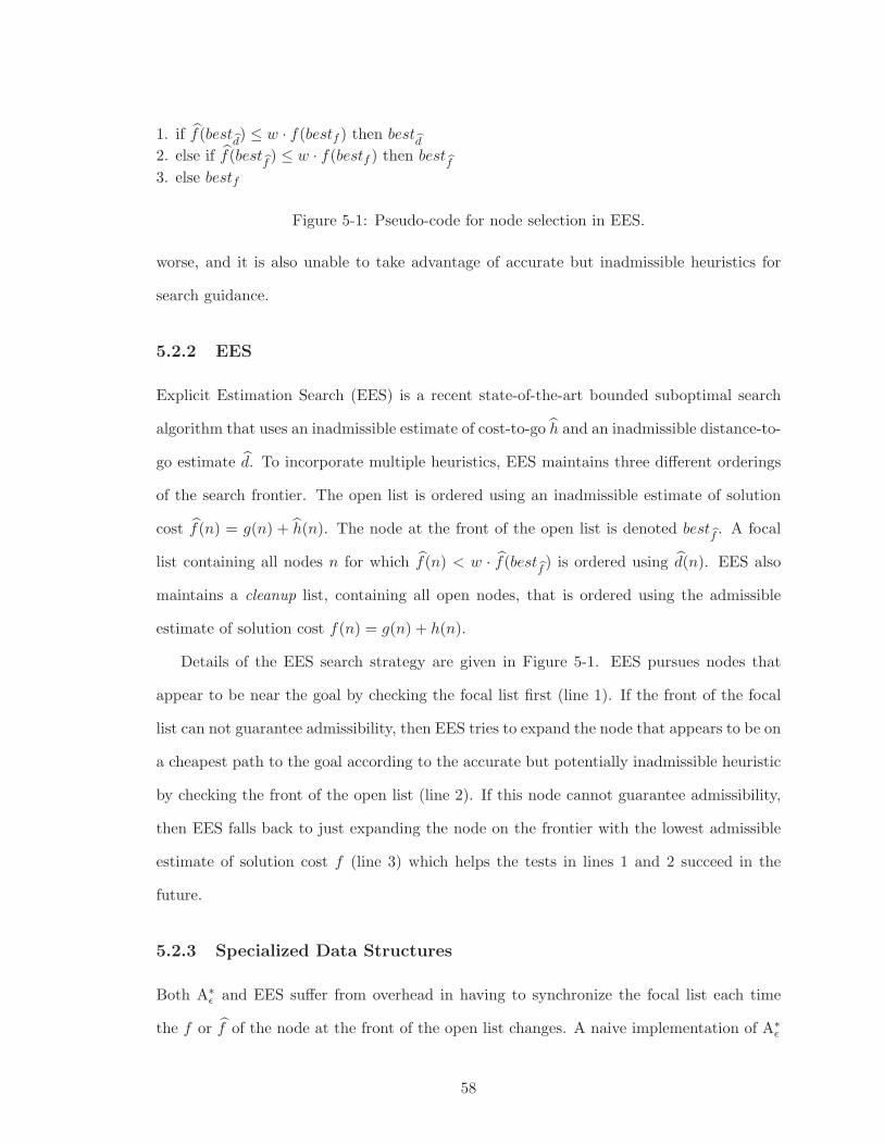
1. if f(bestd) ≤ w · f(bestf ) then best

d

2. else if f(bestf) ≤ w · f(bestf ) then best

f

3. else bestf

Figure 5-1: Pseudo-code for node selection in EES.

worse, and it is also unable to take advantage of accurate but inadmissible heuristics for

search guidance.

5.2.2 EES

Explicit Estimation Search (EES) is a recent state-of-the-art bounded suboptimal search

algorithm that uses an inadmissible estimate of cost-to-go h and an inadmissible distance-to-

go estimate d. To incorporate multiple heuristics, EES maintains three different orderings

of the search frontier. The open list is ordered using an inadmissible estimate of solution

cost f(n) = g(n) + h(n). The node at the front of the open list is denoted bestf. A focal

list containing all nodes n for which f(n) < w · f(bestf) is ordered using d(n). EES also

maintains a cleanup list, containing all open nodes, that is ordered using the admissible

estimate of solution cost f(n) = g(n) + h(n).

Details of the EES search strategy are given in Figure 5-1. EES pursues nodes that

appear to be near the goal by checking the focal list first (line 1). If the front of the focal

list can not guarantee admissibility, then EES tries to expand the node that appears to be on

a cheapest path to the goal according to the accurate but potentially inadmissible heuristic

by checking the front of the open list (line 2). If this node cannot guarantee admissibility,

then EES falls back to just expanding the node on the frontier with the lowest admissible

estimate of solution cost f (line 3) which helps the tests in lines 1 and 2 succeed in the

future.

5.2.3 Specialized Data Structures

Both A∗

ǫ and EES suffer from overhead in having to synchronize the focal list each time

the f or f of the node at the front of the open list changes. A naive implementation of A∗

ǫ

58

or EES would maintain a single list of nodes ordered by f and, for each node expansion,

perform a linear scan of the list to find an admissible node with minimum d. With a loose

upper bound on solution cost, this implementation could visit the entire open list for every

node expansion.

To make A∗

ǫ and EES practical, a more efficient implementation is required (Thayer

et al., 2009). The open list can be represented by a specialized red-black tree and the focal

list can be represented by a binary heap based priority queue. These data structures allow

us to identify the node to expand in constant time, remove it from the focal list and the

open list in logarithmic time, and insert new nodes in logarithmic time.

When the node with minimum f or f changes, nodes may need to be added or removed

from the focal list. To do this efficiently, we do a top-down traversal of the red-black tree,

visiting only the nodes that need to be added or removed. We denote the upper bound

(w · f(bestf ) in the case of A∗

ǫ and w · f(bestf) in the case of EES) for the focal list with b.

For each node expansion we assume that b will not change, and all child nodes that qualify

for the focal list according to the current value of b are added. The value b is updated

only after processing all children. If in fact b does not change, then the focal list is already

synchronized and no further processing is necessary. If b decreases to b′, then a traversal of

the red-black tree is performed, visiting only nodes with a value that is within the interval

of b′ and b. Each visited node is removed from the focal list. If b increases to b′, then a

traversal is performed, visiting only nodes within the interval b and b′, and adding visited

nodes to the focal list.

Unfortunately, even with this optimization, A∗

ǫ and EES can have significant node ex-

pansion overhead compared to single queue based algorithms like WA∗, especially when the

upper bound for the focal list changes frequently. In the worst case, the entire open list

might need to be visited on every node expansion. These algorithms only have a chance

of performing better than WA∗ when distance-to-go estimates and inadmissible heuristics

provide a significant advantage over heuristic guidance alone.

59

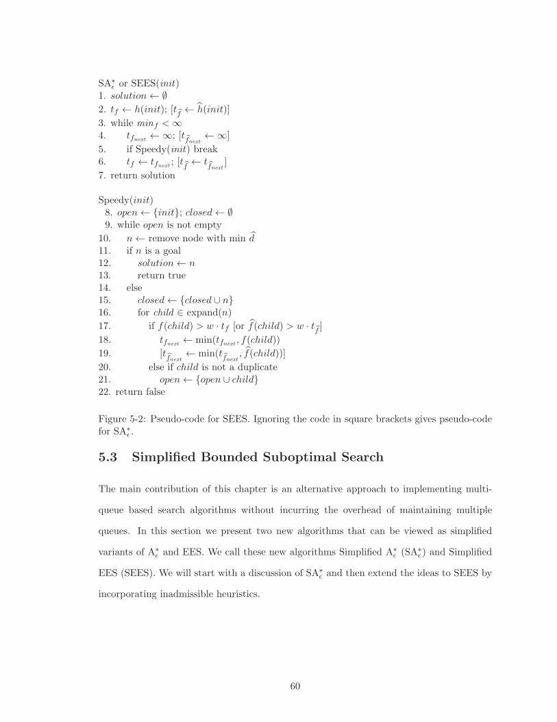
SA∗

ǫ or SEES(init)1. solution← ∅

2. tf ← h(init); [tf← h(init)]

3. while minf <∞4. tfnext ←∞; [t

fnext←∞]

5. if Speedy(init) break6. tf ← tfnext ; [tf ← t

fnext]

7. return solution

Speedy(init)8. open← {init}; closed← ∅9. while open is not empty

10. n← remove node with min d11. if n is a goal12. solution← n13. return true14. else15. closed← {closed ∪ n}16. for child ∈ expand(n)

17. if f(child) > w · tf [or f(child) > w · tf]

18. tfnext ← min(tfnext , f(child))

19. [tfnext← min(t

fnext, f(child))]

20. else if child is not a duplicate21. open← {open ∪ child}22. return false

Figure 5-2: Pseudo-code for SEES. Ignoring the code in square brackets gives pseudo-codefor SA∗

ǫ .

5.3 Simplified Bounded Suboptimal Search

The main contribution of this chapter is an alternative approach to implementing multi-

queue based search algorithms without incurring the overhead of maintaining multiple

queues. In this section we present two new algorithms that can be viewed as simplified

variants of A∗

ǫ and EES. We call these new algorithms Simplified A∗

ǫ (SA∗

ǫ ) and Simplified

EES (SEES). We will start with a discussion of SA∗

ǫ and then extend the ideas to SEES by

incorporating inadmissible heuristics.

60

5.3.1 Simplified A∗

ǫ

A∗

ǫ expands the node with lowest d(n) among those whose f(n) is within a factor w of the

lowest f(n) on open. Intuitively, A∗

ǫ can be viewed as an algorithm that is doing Speedy

search (a best-first search on d (Ruml & Do, 2007)) within an adaptive upper bound on

solution cost. We can approximate this search strategy by using a fixed upper bound that

is updated if the Speedy search fails. This approach, which is less adaptive but has far less

overhead, can be viewed as a combination of iterative deepening (Korf, 1985a) and Speedy

search.

SA∗

ǫ simplifies implementation by eliminating one of the priority queues, namely the open

list, and replaces it with iterative deepening on f . Like IDA∗, SA∗

ǫ maintains a threshold

tf that is initialized to f of the initial state. Search proceeds in iterations, expanding all

nodes with f(n) ≤ w · tf in each iteration. However, unlike IDA∗, within each iteration

nodes are expanded best-first in lowest d(n) order. Nodes that exceed the current upper

bound on solution cost are pruned. At the start of each iteration the threshold is updated

to the minimum cost of all pruned nodes. The completeness of SA∗

ǫ follows easily from the

increasing bound.

The pseudo code for SA∗

ǫ is given in Figure 5-2, ignoring the code in brackets. SA∗

ǫ

begins by computing h of the initial state to initialize the tf threshold (line 2). Next, search

proceeds by performing a bounded speedy search (lines 3–5). The initial state is added to

the open list, a priority queue that is sorted by d(n) (line 8). The speedy search proceeds by

expanding the best node on open, pruning all child nodes where f(n) exceeds the current

tf threshold (lines 15-21). The minimum f(n) of all pruned nodes is remembered at each

iteration and is used as the threshold for the next iteration (lines 4, 18 and 6). At each

iteration, SA∗

ǫ prunes all nodes with f(n) > w · tf (line 17). If the heuristic is admissible,

SA∗

ǫ can terminate when a goal node is expanded and guarantee that the cost of the solution

is w-admissible (lines 11-13). If a goal is not found in one iteration, the threshold is updated

(line 6) and the speedy search repeats.

Theorem 2 If SA∗

ǫ terminates with a solution, it is w-admissible if the heuristic is admis-

61

sible.

Proof: Let C be the cost of the goal returned by SA∗

ǫ and assume for the sake of

contradiction that C > w · C∗. Let ti be the threshold used in the iteration when the goal

node was expanded. Since the goal node was expanded, it holds that C ≤ w · ti. On the

other hand, the goal was not expanded in the previous iteration, where the threshold was

lower than ti. Since ti is updated to be the minimum f value of all nodes that exceeded

the previous bound, then at least one node p that is on the optimal path to the goal has

f(p) ≥ w · ti. Therefore:

C ≤ w · ti ≤ w · f(p)

≤ w · (g(p) + h(p)) ≤ w · C∗

This contradicts the assumption that C > w · C∗. �

SA∗

ǫ approximates the search behavior of A∗

ǫ by expanding nodes that appear to be closer

to the goal first, among those nodes that guarantee admissibility. Because SA∗

ǫ expands only

nodes that guarantee admissibility, it can terminate as soon as it expands a goal, just like

A∗

ǫ . Unlike A∗

ǫ , which adaptively sets the upper bound for the focal list, potentially at each

node expansion, SA∗

ǫ uses a fixed upper bound at each iteration and must exhaust all nodes

in the focal list before increasing this bound.

5.3.2 Simplified EES

A∗

ǫ and EES have similar motivations, and both algorithms perform a speedy search within

an adaptive upper bound on solution cost. We refer to the nodes that are within the upper

bound as the search envelope. EES differs from A∗

ǫ in that it incorporates an accurate but

potentially inadmissible heuristic h to help shape the search envelope. This inadmissible

heuristic helps by pruning nodes from the search envelope that would otherwise be ex-

panded by A∗

ǫ . To approximate the search strategy of EES, we can apply the same iterative

deepening technique of SA∗

ǫ . However, this time we need to perform iterative deepening

62

on two upper bounds: the upper bound on solution cost f and the upper bound on the

inadmissible estimate of solution cost f .

SEES orders node expansions according to d(n) and prunes nodes with high f(n) and

f(n). This emulates the same criteria used to determine which nodes form the focal list

in EES and which nodes are selected for expansion (Figure 5-1). However, one critical

difference is that SEES only ever expands nodes from the focal list, because all nodes in

the focal list are w-admissible. In contrast, not all nodes that form the focal list for EES

guarantee admissibility and EES can potentially expand nodes from either of three priority

queues during search.

The pseudo code for SEES is given in Figure 5-2 including the code in square brackets.

SEES is the same algorithm as SA∗

ǫ with the addition of an inadmissible node evaluation

function for pruning (lines 2, 4, 6, 17 and 19). Compared to EES, the priority queue for the

open list is replaced by iterative deepening on f and the priority queue for the cleanup list

is replaced by iterative deepening on f . This leaves just one priority queue, the focal list,

ordered by d(n). The proof for EES being w-admissible is identical to the proof for SA∗

ǫ .

SA∗

ǫ and SEES have far less overhead than their progenitors. Each requires only a single

priority queue, sorted according to one evaluation function. Each node only needs to be

stored in one priority queue, requiring less memory to store each node. Moreover, the focal

list does not need to be synchronized.

5.4 Empirical Evaluation

While the new algorithms adhere to the intent behind the originals, the emulation is only

approximate. To determine the effectiveness of the simplified approach, we implemented

SA∗

ǫ and SEES and compared them to A∗

ǫ , EES and WA∗ on 4 different domains, including

3 of the simplest and most reproducible of the original 6 domains used by Thayer and

Ruml (2010). For all experiments, we used path-based single step error correction of the

admissible heuristic h to construct a more accurate but potentially inadmissible heuristic h,

as described by Thayer and Ruml (2010). All algorithms were written in Java and compiled

63

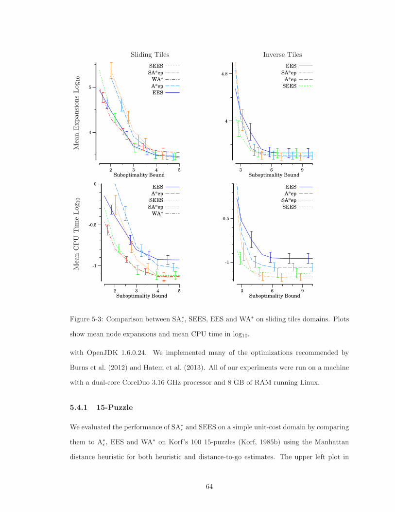
Sliding Tiles Inverse Tiles

MeanExpan

sion

sLog

10

Suboptimality Bound5432

5

4

SEES

SA*ep

WA*

A*ep

EES

Suboptimality Bound963

4.8

4

EES

SA*ep

A*ep

SEES

MeanCPU

Tim

eLog

10

Suboptimality Bound5432

0

-0.5

-1

EES

A*ep

SEES

SA*ep

WA*

Suboptimality Bound963

-0.5

-1

EES

A*ep

SA*ep

SEES

Figure 5-3: Comparison between SA∗

ǫ , SEES, EES and WA∗ on sliding tiles domains. Plots

show mean node expansions and mean CPU time in log10.

with OpenJDK 1.6.0.24. We implemented many of the optimizations recommended by

Burns et al. (2012) and Hatem et al. (2013). All of our experiments were run on a machine

with a dual-core CoreDuo 3.16 GHz processor and 8 GB of RAM running Linux.

5.4.1 15-Puzzle

We evaluated the performance of SA∗

ǫ and SEES on a simple unit-cost domain by comparing

them to A∗

ǫ , EES and WA∗ on Korf’s 100 15-puzzles (Korf, 1985b) using the Manhattan

distance heuristic for both heuristic and distance-to-go estimates. The upper left plot in

64

Figure 5-3 shows mean node expansions at suboptimality bounds 1.5, 2, 3, 4 and 5. As

the suboptimality bound increases, each algorithm requires fewer node expansions and all

algorithms require roughly the same number of node expansions beyond a suboptimality

bound of 3. However, when we examine solving times, the lower left plot, we see that

EES and A∗

ǫ are significantly slower overall while SEES performs as well as WA∗. EES

performs poorly compared to SEES and WA∗ because the overhead of maintaining multiple

orderings of the search frontier outweighs the benefits of the search guidance provided by

the inadmissible heuristic h. The node expansion rate for SEES is roughly 2.5 times faster

than EES in this setting. SA∗

ǫ is faster than A∗

ǫ but the difference is not as dramatic.

Next, we change the domain slightly by modifying the cost function such that the

cost to move a tile is the inverse of the number on the face of the tile. This provides

a wide range of edge costs in a simple, well understood domain. Moreover, distance-to-go

estimates provide a significant advantage over using the Manhattan distance heuristic alone.

In this domain WA∗ is not able to solve all instances with our timeout of 60 seconds at

any suboptimality bound. The plots in the second column in Figure 5-3 show that while

SA∗

ǫ expands roughly the same nodes as its progenitor, it solves problems faster as the

bound loosens. SEES is the fastest algorithm at lower suboptimality bounds. All these

algorithms are able to dramatically outperform WA∗ on this domain because they are able

to incorporate distance-to-go estimates for search guidance.

These plots provide evidence that SEES is merely an approximation to EES, as it ex-

pands fewer nodes on average in this domain. We believe the difference in node expansions

can be attributed to the non-monotonic upper bounds. While SEES uses fixed upper bounds

that never decrease, EES sets this bound adaptively. Since the upper bounds never decrease

for SEES, it may be able to find admissible paths to a goal sooner than EES.

5.4.2 Pancake Puzzle

We also evaluated the performance of these algorithms on the heavy pancake puzzle using

the gap heuristic. In this domain we must order a stack of pancakes labeled {1, ..., N},

65

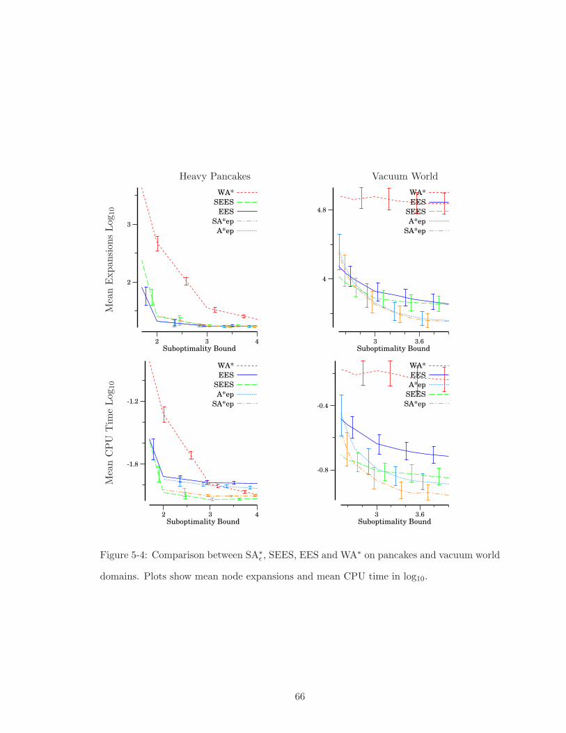
Heavy Pancakes Vacuum World

MeanExpan

sion

sLog

10

Suboptimality Bound432

3

2

WA*

SEES

EES

SA*ep

A*ep

Suboptimality Bound3.63

4.8

4

WA*

EES

SEES

A*ep

SA*ep

MeanCPU

Tim

eLog

10

Suboptimality Bound432

-1.2

-1.8

WA*

EES

SEES

A*ep

SA*ep

Suboptimality Bound3.63

-0.4

-0.8

WA*

EES

A*ep

SEES

SA*ep

Figure 5-4: Comparison between SA∗

ǫ , SEES, EES and WA∗ on pancakes and vacuum world

domains. Plots show mean node expansions and mean CPU time in log10.

66

where N is the number of pancakes, by reversing a contiguous prefix (flipping a subset of

the stack). The gap heuristic is a type of landmark heuristic that counts the number of non

adjacent pancakes or “gaps” for each pancake in the stack (Helmert, 2010). This heuristic

has been shown to be very accurate, outperforming abstraction based heuristics. In heavy

pancakes, the cost to flip a stack of pancakes is the sum of the pancake ids in the stack. This

produces a wide range of integer edge costs and distance-to-go estimates provide additional

search guidance over using the heuristic alone. In our experiments we used 100 random

instances with 14 pancakes. For the admissible heuristic, we adapted the gap heuristic

and we used the basic unit cost form of the gap heuristic for the distance-to-go estimate.

The plots in the first column of Figure 5-4 show the number of node expansions and the

mean solving time. WA∗ is the worst performing algorithm and A∗

ǫ and SA∗

ǫ were only able

to solve all instances within our memory limit of 8GB or our timeout of 500 seconds for

suboptimality bounds greater than 2. In this domain SEES expands more nodes than EES.

This is because at lower suboptimality bounds, SEES performs many iterations, resulting in

many node re-expansions. However, SEES still solves problems as fast or faster than EES

because it has significantly less overhead per expansion. SA∗

ǫ is faster than A∗

ǫ but again

the difference is not as dramatic.

5.4.3 Vacuum World

The Vacuum World domain is the first state space introduced in Russell and Norvig (2003).

In this domain a vacuum robot must clean up dirt distributed across a grid world. In

the version considered here, actions have different costs depending on how much dirt the

robot is carrying. This variant is called the Heavy Vacuum World. In our experiments

we used the same heuristic and distance estimates used by Thayer and Ruml (2010). The

admissible heuristic is computed by finding a minimum spanning tree for all remaining dirt

piles, ignoring blocked locations. The edges of the tree are sorted by decreasing length

and we sum the product of each edge and weight of the robot, starting with the current

weight and increasing it for each edge. The distance-to-go estimate is a greedy traversal of

67

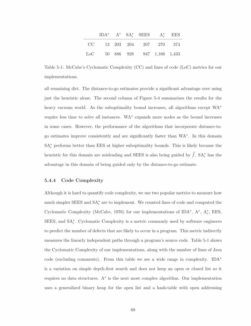
IDA∗ A∗ SA∗

ǫ SEES A∗

ǫ EES

CC 13 203 204 207 270 374

LoC 50 886 928 947 1,166 1,433

Table 5-1: McCabe’s Cyclomatic Complexity (CC) and lines of code (LoC) metrics for our

implementations.

all remaining dirt. The distance-to-go estimates provide a significant advantage over using

just the heuristic alone. The second column of Figure 5-4 summarizes the results for the

heavy vacuum world. As the suboptimality bound increases, all algorithms except WA∗

require less time to solve all instances. WA∗ expands more nodes as the bound increases

in some cases. However, the performance of the algorithms that incorporate distance-to-

go estimates improve consistently and are significantly faster than WA∗. In this domain

SA∗

ǫ performs better than EES at higher suboptimality bounds. This is likely because the

heuristic for this domain are misleading and SEES is also being guided by f . SA∗

ǫ has the

advantage in this domain of being guided only by the distance-to-go estimate.

5.4.4 Code Complexity

Although it is hard to quantify code complexity, we use two popular metrics to measure how

much simpler SEES and SA∗

ǫ are to implement. We counted lines of code and computed the

Cyclomatic Complexity (McCabe, 1976) for our implementations of IDA∗, A∗, A∗

ǫ , EES,

SEES, and SA∗

ǫ . Cyclomatic Complexity is a metric commonly used by software engineers

to predict the number of defects that are likely to occur in a program. This metric indirectly

measures the linearly independent paths through a program’s source code. Table 5-1 shows

the Cyclomatic Complexity of our implementations, along with the number of lines of Java

code (excluding comments). From this table we see a wide range in complexity. IDA∗

is a variation on simple depth-first search and does not keep an open or closed list so it

requires no data structures. A∗ is the next most complex algorithm. Our implementation

uses a generalized binary heap for the open list and a hash-table with open addressing

68

and quadratic collision resolution. SEES and SA∗

ǫ are just slightly more complex than A∗.

They use the same binary heap and hash-table for the open and closed lists. EES is by

far the most complex program. It uses the same binary heap and hash-table from our A∗

implementation but also requires a red-black tree to store the open list. SEES represents a

45% reduction in complexity over EES and SA∗

ǫ represents a 24% reduction in complexity

over A∗

ǫ .

5.5 Discussion

While we have focused on presenting very simple alternatives to A∗

ǫ and EES, optimizations

are possible that will further improve performance in certain situations.

Thayer and Ruml (2010) present an optimistic variant of EES, EESopt, that borrows

ideas from Optimistic Search (Thayer & Ruml, 2008), a bounded suboptimal search al-

gorithm that ignores the admissible evaluation function until an incumbent solution is

found. After an incumbent is found, a cleanup search phase uses the admissible heuristic

to prove the incumbent is w-admissible. Like Optimistic Search, EESopt ignores the admis-

sible heuristic, expanding just nodes in the focal list until an incumbent is found. Once

an incumbent is found EESopt proceeds just like EES until f(incumbent) ≤ w · f(bestf ).

We can use a similar technique to formulate an optimistic variant of SEES (SEESopt). We

do this by simply ignoring the ft threshold until an incumbent solution is found. Once an

incumbent is found SEESopt proceeds just like SEES until it can prove the incumbent is

w-admissible or until it finds a new incumbent that is. This is advantageous when h is very

accurate.

SA∗

ǫ and SEES use an iterative deepening search strategy inspired by IDA∗. Like IDA∗,

SA∗

ǫ and SEES expand a super-set of the nodes in the previous iteration. If the size of iter-

ations grows geometrically, then the node regeneration overhead is bounded by a constant.

In domains with a wide distribution of edge costs, there can be many unique f values and

the standard minimum-out-of-bound threshold updates may lead to only a few new nodes

being expanded in each iteration. The number of nodes expanded by IDA∗ can be O(n2)

69

(Sarkar et al., 1991) in the worst case when the number of new nodes expanded in each

iteration is constant. To alleviate this problem, Sarkar et al. introduce IDA*CR. IDA*CR

tracks the distribution of f values of the pruned nodes during an iteration of search and uses

it to find a good threshold for the next iteration. This is achieved by selecting the bound

that will cause the desired number of pruned nodes to be expanded in the next iteration.

We can apply a similar technique to SA∗

ǫ and SEES. However, because SEES uses

two thresholds for pruning, a special two-dimensional binning is required. Each of the

upper bounds tf and tf, defines a set of nodes that qualify for expansion according to that

threshold. SEES expands just the intersection of these two sets. Tracking the distribution of

f and f in separate histograms does not provide the same guarantee for the desired number

of expansions. A two-dimensional binning tracks f along one dimension and f along the

other dimension. Selecting thresholds according to this two dimensional binning allows for

the same guarantee as the original one-dimensional CR technique. We did not use any of

these techniques in our experiments since we did not find node re-expansion overhead to

result in worse performance for SA∗

ǫ and SEES when compared to their progenitors.

We can eliminate all node re-expansion caused by iterative deepening by simply re-

membering search progress between iterations. Rather than deleting nodes that exceed the

current thresholds, they are placed on a separate open list for the next iteration. The closed

list persists across all iterations. This technique is reminiscent of Fringe search (Bjornsson

et al., 2005), an algorithm that has been shown to perform better than A∗ in some domains

by replacing the priority queue with a iterative layered search. This optimization adds

complexity to the implementation and we did not use it in any of our experiments.

5.6 Conclusion

In this chapter, we presented simplified variants of A∗

ǫ (SA∗

ǫ ) and EES (SEES) that use

a different implementation of the same fundamental ideas to significantly reduce search

overhead and implementation complexity. In an empirical evaluation, we showed that SA∗

ǫ

and SEES, like the originals, outperform other bounded suboptimal search algorithms, such

70

as WA∗. We also confirmed that, while SA∗

ǫ and SEES expand roughly the same number

of nodes as the originals, they solve problems significantly faster, setting a new state-of-

the-art in our benchmark domains, and they are significantly easier to implement. This

work provides a general approach that may be applicable to other complex multi-queue

based search algorithms. We hope this work leads to faster, simplified and wider adoption

of inadmissible heuristics and distance estimates in bounded suboptimal search.

71

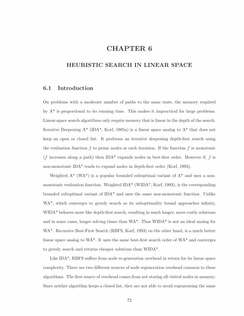
CHAPTER 6

HEURISTIC SEARCH IN LINEAR SPACE

6.1 Introduction

On problems with a moderate number of paths to the same state, the memory required

by A* is proportional to its running time. This makes it impractical for large problems.

Linear-space search algorithms only require memory that is linear in the depth of the search.

Iterative Deepening A* (IDA*, Korf, 1985a) is a linear space analog to A* that does not

keep an open or closed list. It performs an iterative deepening depth-first search using

the evaluation function f to prune nodes at each iteration. If the function f is monotonic

(f increases along a path) then IDA* expands nodes in best-first order. However if, f is

non-monotonic IDA* tends to expand nodes in depth-first order (Korf, 1993).

Weighted A* (WA*) is a popular bounded suboptimal variant of A* and uses a non-

monotonic evaluation function. Weighted IDA* (WIDA*, Korf, 1993), is the corresponding

bounded suboptimal variant of IDA* and uses the same non-monotonic function. Unlike

WA*, which converges to greedy search as its suboptimality bound approaches infinity,

WIDA* behaves more like depth-first search, resulting in much longer, more costly solutions

and in some cases, longer solving times than WA*. Thus WIDA* is not an ideal analog for

WA*. Recursive Best-First Search (RBFS, Korf, 1993) on the other hand, is a much better

linear space analog to WA*. It uses the same best-first search order of WA* and converges

to greedy search and returns cheaper solutions than WIDA*.

Like IDA*, RBFS suffers from node re-generation overhead in return for its linear space

complexity. There are two different sources of node regeneration overhead common to these

algorithms. The first source of overhead comes from not storing all visited nodes in memory.

Since neither algorithm keeps a closed list, they are not able to avoid regenerating the same

72

nodes through multiple paths. This limits IDA* and RBFS to problems where each state is

reachable by relatively few paths. The second source of overhead, and one that we discuss

in more detail in this chapter, comes from having to regenerate the same nodes in each

successive iteration of IDA* or each time a subtree is revisited in RBFS. The contributions

of this chapter address this source of overhead for RBFS.

While the per iteration node re-generation overhead of IDA* is easily characterized

in terms of the heuristic branching factor, the overhead of RBFS depends on how widely

separated nodes of successive cost are in the tree. Moreover, as we explain below, RBFS

fails on domains that exhibit a large range of f values. The main contribution of this

chapter is a set of techniques for improving the performance of RBFS. We start with two

simple techniques that perform well in practice but provide no theoretical guarantees on

performance. We present a third technique that is more complex to implement but performs

well in practice and comes with a bound on re-expansion overhead, making it the first linear

space best-first search robust enough to solve a variety of domains with varying operator

costs. While IDA* enjoys widespread popularity, this work indicates that it may be time

for a re-assessment of RBFS.

6.2 Previous Work

6.2.1 Iterative Deepening A*

IDA* was described previously in chapter 3 but we describe it again in this chapter with

relevant details. IDA* performs iterations of bounded depth-first search where a path

is pruned if f(n) becomes greater than the bound for the current iteration. After each

unsuccessful iteration, the bound is increased to the minimum f value among the nodes

that were generated but not expanded in the previous iteration. Each iteration of IDA*

expands a super set of the nodes in the previous iteration. If the size of iterations grows

geometrically, then the number of nodes expanded by IDA* is O(N), where N is the number

of nodes that A* would expand (Sarkar et al., 1991).

73

In domains with a wide range of edge costs, there can be many unique f values and the

standard minimum-out-of-bound bound schedule of IDA* may lead to only a few new nodes

being expanded in each iteration. The number of nodes expanded by IDA* can be O(n2)

(Sarkar et al., 1991) in the worst case when the number of new nodes expanded in each

iteration is constant. To alleviate this problem, Sarkar et al. introduce IDA*CR. IDA*CR

tracks the distribution of f values of the pruned nodes during an iteration of search and uses

it to find a good threshold for the next iteration. This is achieved by selecting the bound

that will cause the desired number of pruned nodes to be expanded in the next iteration. If

the successors of these pruned nodes are not expanded in the next iteration, then this scheme

is able to accurately double the number of nodes between iterations. If the successors do

fall within the bound on the next iteration, then more nodes may be expanded than desired

but this is often not harmful in practice (Burns & Ruml, 2013). Since the threshold is

increased liberally, the search order is no longer best-first and branch-and-bound must be

used on the final iteration of search to ensure optimality. When a goal node is generated

the current threshold is updated to be the cost of the goal and the IDA* search continues.

If a better goal is found the threshold is updated again. Otherwise IDA* terminates once

all nodes within the threshold are expanded.

Weighting the heuristic in IDA* results in Weighted IDA* (WIDA*): a bounded sub-

optimal linear space search algorithm using the non-monotonic cost function f ′(n) =

g(n) + w · h(n). As w increases, WIDA* prunes large portions of the search space and is

often able to find w-admissible solutions quickly. However, the remaining paths are searched

in depth-first order, resulting in significantly more expensive solutions and in some cases,

longer solving times. In contrast, WA* performs more like greedy search as the bound

increases and it finds cheaper solutions. Thus WIDA* is not an ideal analog for WA*.

6.2.2 Recursive Best-First Search

Unlike IDA*, RBFS expands nodes in best-first order even with a non-monotonic cost

function. The pseudo-code for RBFS is shown in Figure 6-1. RBFS recursively expands

74

RBFS(n, B)1. if n is a goal2. solution← n; return ∞3. C ← expand(n)4. if C is empty return ∞5. for each child ni in C6. if f(n) < F (n) then F (ni)← max(F (n), f(ni))7. else F (ni)← f(ni)8. sort C in increasing order of F9. if |C| = 1 then F (C[2])←∞

10. while (F (C[1]) ≤ B and F (C[1]) <∞)11. F (C[1])← RBFS(C[1], min(B,F (C[2])))12. resort C13. return F (C[1])

Figure 6-1: Pseudo-code for RBFS.

nodes (line 3 and 11), ordering child nodes by cost (line 8) and expanding the least cost

children first. Each recursive call uses a local threshold B that is the minimum cost of

a node generated so far but not yet expanded in another branch of the search tree. This

defines a virtual frontier for the search. If all child costs exceed the local threshold, the

search backtracks (lines 10 and 13). Each time RBFS backtracks from a parent node, it

backs up the cost of the best child that exceeded the local threshold (line 11). This allows

the search to quickly pickup where it left off when revisiting that sub-tree. When RBFS

expands a goal node it can terminate (lines 1 and 2).

RBFS backtracks from a node n as soon as all descendants of a n have an F greater than

the threshold B. If B takes on a wide range of values, then RBFS can suffer from excessive

backtracking. In the worst case, every node may have a unique f value with successive values

located in separate subtrees, in which case RBFS would backtrack at every node expansion

and regenerate all previously generated nodes before expanding a new node, resulting in

O(N2) expansions. RBFS is often slower than WIDA* however, it finds cheaper solutions,

matching the cost of solutions returned by WA* on average, making it a better WA* analog.

This overhead depends on how widely separated nodes of successive cost are in the tree.

75

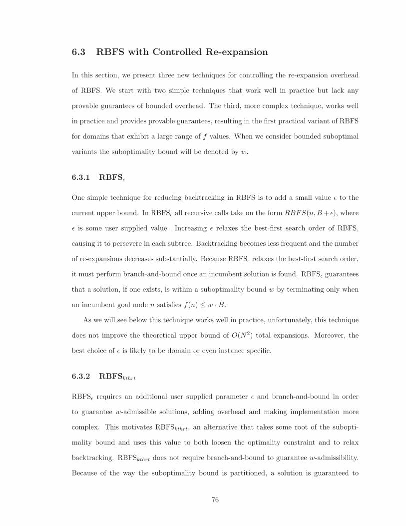
6.3 RBFS with Controlled Re-expansion

In this section, we present three new techniques for controlling the re-expansion overhead

of RBFS. We start with two simple techniques that work well in practice but lack any

provable guarantees of bounded overhead. The third, more complex technique, works well

in practice and provides provable guarantees, resulting in the first practical variant of RBFS

for domains that exhibit a large range of f values. When we consider bounded suboptimal

variants the suboptimality bound will be denoted by w.

6.3.1 RBFSǫ

One simple technique for reducing backtracking in RBFS is to add a small value ǫ to the

current upper bound. In RBFSǫ all recursive calls take on the form RBFS(n,B+ ǫ), where

ǫ is some user supplied value. Increasing ǫ relaxes the best-first search order of RBFS,

causing it to persevere in each subtree. Backtracking becomes less frequent and the number

of re-expansions decreases substantially. Because RBFSǫ relaxes the best-first search order,

it must perform branch-and-bound once an incumbent solution is found. RBFSǫ guarantees

that a solution, if one exists, is within a suboptimality bound w by terminating only when

an incumbent goal node n satisfies f(n) ≤ w ·B.

As we will see below this technique works well in practice, unfortunately, this technique

does not improve the theoretical upper bound of O(N2) total expansions. Moreover, the

best choice of ǫ is likely to be domain or even instance specific.

6.3.2 RBFSkthrt

RBFSǫ requires an additional user supplied parameter ǫ and branch-and-bound in order

to guarantee w-admissible solutions, adding overhead and making implementation more

complex. This motivates RBFSkthrt, an alternative that takes some root of the subopti-

mality bound and uses this value to both loosen the optimality constraint and to relax

backtracking. RBFSkthrt does not require branch-and-bound to guarantee w-admissibility.

Because of the way the suboptimality bound is partitioned, a solution is guaranteed to

76

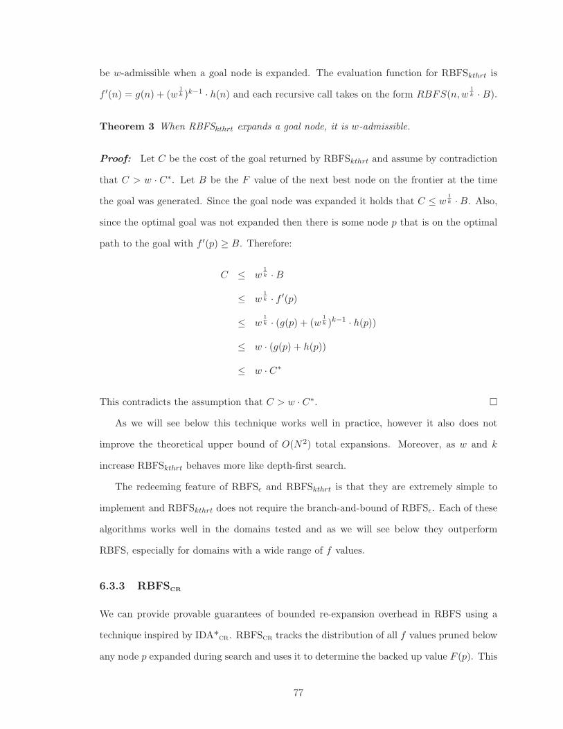
be w-admissible when a goal node is expanded. The evaluation function for RBFSkthrt is

f ′(n) = g(n) + (w1

k )k−1 · h(n) and each recursive call takes on the form RBFS(n,w1

k ·B).

Theorem 3 When RBFSkthrt expands a goal node, it is w-admissible.

Proof: Let C be the cost of the goal returned by RBFSkthrt and assume by contradiction

that C > w · C∗. Let B be the F value of the next best node on the frontier at the time

the goal was generated. Since the goal node was expanded it holds that C ≤ w1

k ·B. Also,

since the optimal goal was not expanded then there is some node p that is on the optimal

path to the goal with f ′(p) ≥ B. Therefore:

C ≤ w1

k ·B

≤ w1

k · f ′(p)

≤ w1

k · (g(p) + (w1

k )k−1 · h(p))

≤ w · (g(p) + h(p))

≤ w · C∗

This contradicts the assumption that C > w · C∗. �

As we will see below this technique works well in practice, however it also does not

improve the theoretical upper bound of O(N2) total expansions. Moreover, as w and k

increase RBFSkthrt behaves more like depth-first search.

The redeeming feature of RBFSǫ and RBFSkthrt is that they are extremely simple to

implement and RBFSkthrt does not require the branch-and-bound of RBFSǫ. Each of these

algorithms works well in the domains tested and as we will see below they outperform

RBFS, especially for domains with a wide range of f values.

6.3.3 RBFSCR

We can provide provable guarantees of bounded re-expansion overhead in RBFS using a

technique inspired by IDA*CR. RBFSCR tracks the distribution of all f values pruned below

any node p expanded during search and uses it to determine the backed up value F (p). This

77

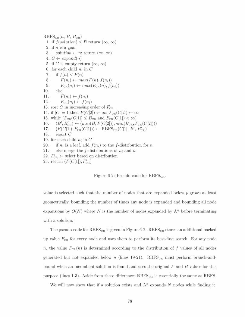
RBFSCR(n, B, BCR)1. if f(solution) ≤ B return (∞, ∞)2. if n is a goal3. solution← n; return (∞, ∞)4. C ← expand(n)5. if C is empty return (∞, ∞)6. for each child ni in C7. if f(n) < F (n)8. F (ni)← max(F (n), f(ni))9. FCR(ni)← max(FCR(n), f(ni))

10. else11. F (ni)← f(ni)12. FCR(ni)← f(ni)13. sort C in increasing order of FCR

14. if |C| = 1 then F (C[2])←∞; FCR(C[2])←∞15. while (FCR(C[1]) ≤ BCR and FCR(C[1]) <∞)16. (B′, B′

CR)← (min(B,F (C[2])),min(BCR, FCR(C[2])))

17. (F (C[1]), FCR(C[1]))← RBFSCR(C[1], B′, B′

CR)

18. resort C19. for each child ni in C20. if ni is a leaf, add f(ni) to the f -distribution for n21. else merge the f -distributions of ni and n22. F ′

CR← select based on distribution

23. return (F (C[1]), F ′

CR)

Figure 6-2: Pseudo-code for RBFSCR.

value is selected such that the number of nodes that are expanded below p grows at least

geometrically, bounding the number of times any node is expanded and bounding all node

expansions by O(N) where N is the number of nodes expanded by A* before terminating

with a solution.

The pseudo-code for RBFSCR is given in Figure 6-2. RBFSCR stores an additional backed

up value FCR for every node and uses them to perform its best-first search. For any node

n, the value FCR(n) is determined according to the distribution of f values of all nodes

generated but not expanded below n (lines 19-21). RBFSCR must perform branch-and-

bound when an incumbent solution is found and uses the original F and B values for this

purpose (lines 1-3). Aside from these differences RBFSCR is essentially the same as RBFS.

We will now show that if a solution exists and A* expands N nodes while finding it,

78

then RBFSCR will only expand O(N) nodes. The proof relies on the same assumptions of

IDA*CR which we include below for correctness and clarity.

Assumption 1 The number of unique nodes n such that C∗ < f(n) ≤ f(q) is O(N) where

q is the node with the largest f generated during search and N is the number of nodes

expanded by A* when no duplicates are pruned and with worst-case tie-breaking.

This assumption is reasonable, for example, in domains in which g and h values are com-

puted in terms of the costs of a fixed set of operators. This often implies that f values

increase by bounded amounts and that the number of nodes in successive f layers are

related by a constant (known as the heuristic branching factor Korf & Reid, 1998).

Assumption 2 The number of leaf nodes generated below every subtree is sufficient to

support geometric growth.

This assumption is reasonable, as the counter example is a search tree with very few

branches. This kind of problem would not warrant linear-space search to begin with and is

not relevant to our study.

Lemma 4 Consider the search as it enters a subtree rooted at node p. Let the next best

node on the virtual frontier be q. If FCR(q) ≤ C∗, then only nodes n such that f(n) ≤ C∗

are expanded below p.

Proof: The proof for this follows from similar reasoning as Lemma 4.1 in Korf (1993).

FCR(q) bounds the expansions performed in p. The search backtracks from p once all nodes

n such that f(n) ≤ FCR(q) below p have been expanded and it does not expand any nodes

n such that f(n) > FCR(q). Since FCR(q) ≤ C∗ then all expanded nodes have f(n) ≤ C∗. �

We will assume that the distributions maintained by RBFSCR suffer no loss in precision.

Lemma 5 Consider any subtree rooted at a node p. The value FCR(p) always increases

monotonically.

79

Proof: FCR(p) is always updated with a value that is larger than the previous one. Fringe

nodes p′ below p whose f values exceed FCR(p) are added to a histogram and used to set

FCR(p). All of the fringe nodes in the histogram have an f that exceeds FCR(p). Let F′

CR(p)

be the updated value for FCR(p). We set F ′

CR(p) such that there is at least one fringe node

p with f(p) ≤ F ′

CR(p). Therefore, FCR(p) < F ′

CR(p). �

Lemma 6 Consider the search as it enters a subtree rooted at node p. Let the next best

node on the virtual frontier be q. Every node in the subtree with f(n) ≤ F (p) will be explored

and nodes that have already been expanded will be re-expanded only once before the search

backtracks to p.

Proof: The value FCR(q) bounds the expansions performed in p. The best-first search

order guarantees that FCR(p) ≤ FCR(q). The search will not backtrack from the subtree

until at least all nodes p′ below p with f(p′) ≤ FCR(p) (and no nodes n in the path to

them with f(n) > FCR(p)) have been expanded. All nodes p′ below p that were already

expanded previously have FCR(p′) = max(FCR(p), f(p

′)) (lines 7-9) and all recursive calls

below node p have the form RBFSCR(p,B) for some B, where FCR(p) ≤ FCR(p′) ≤ B. Since

FCR(p) ≤ FCR(p′) and FCR(p

′) is guaranteed to increase for each call to RBFSCR(p′, B) by

Lemma 5, it follows that any node p′ below p will not qualify for re-expansion until the

search backtracks to p. �

Lemma 7 : The total number of unique nodes visited during search is bounded by O(N).

Proof: Consider all nodes n expanded by the search and let node q be the generated

node with the highest f value. Either f(n) ≤ C∗ or C∗ < f(n) ≤ f(q). The total number

of unique nodes n with f(n) ≤ C∗ is at most N . The total number of unique nodes with

C∗ < f(n) ≤ f(q) is O(N) by Assumption 1. Thus, the total number of unique nodes

visited by the search is N +O(N) = O(N). �

Lemma 8 At least as many nodes are expanded below a subtree p as we anticipated when

selecting FCR(p).

80

Proof: Since FCR(p) < F ′

CR(p) by Lemma 5, when we expand p with F ′

CR(p) we will expand

all the nodes expanded when expanding p with FCR(p) (see also Lemma 6). Furthermore,

the fringe nodes p′, whose f values were added to the distribution last time and used to

compute F ′

CR(p), and that we anticipated would fall below FCR(p), will be initialized with

FCR(p′) = f(p′) in line 12, so they will pass the test in line 15 and be expanded in the call

at line 17. �

Lemma 9 RBFSCR will terminate with a solution if one exists.

Proof: From Lemma 5 and Lemma 8 the bound at each subtree is always increasing

and all nodes below the bound are expanded during search. Eventually the bound when

exploring a subtree is larger than or equal to the cost of a solution and a goal node is

expanded. �

Theorem 4 If a solution exists and A* expands N nodes before terminating with a solution,

then RBFSCR expands O(N) nodes before terminating with a solution.

Proof: From Lemma 9 we already proved completeness so we need only show an upper

bound on re-expansion overhead. With Assumption 2, FCR(p) is set when backtracking to

cause at least twice as many nodes to be expanded the next time p is expanded, and by

Lemma 8 at least this many nodes will be expanded, then by Lemma 6 each node previously

expanded below p is expanded exactly one more time when we enter the subtree at p. This

implies that the number of nodes expanded is at least doubling. We can’t expand a node a

second time without expanding at least one new node for the first time. Furthermore, when

we expand a node that had been expanded twice for a third time, we also expand all the

nodes below it that had been expanded once for a second time, and then expand a number

of nodes for the first time that is at least the sum of the number of nodes expanded for a

third or second time. In general, let si be the set of nodes that have been expanded i times

and let ni = |si|. The sizes of these sets form a series in which ni+1 ≤ ni/2.

Because every unique node expanded is expanded some number of times, the total

number of unique nodes expanded is the value∑

∞

i ni. The total number of expansions

81

(including re-expansions) is:

∑∞

i=1 i(ni) ≤ 1(n1) + 2(n1

2 ) + 3(n1

4 ) + 4(n1

8 ) + ...

≤∑

∞

i=1 i(n1/2(i−1))

≤ 2n1∑

∞

i=1 i(2−i)

< 4n1

By Lemma 7, n1 = O(N), so the total number of expansions is also O(N). �

6.4 Empirical Evaluation

We compared the new algorithms to RBFS and WIDA* (and WIDA*CR) on the clas-

sic sliding tiles problem using a variety of edge cost functions. For RBFSǫ we tried

ǫ = {1, 2, 4, 8, 16} and for RBFSkthrt we tried i = {2, 5, 10}. Unless noted, each algorithm

was given five minutes to provide a solution before being terminated for each instance in

the set. All algorithms were written in Java and compiled with OpenJDK 1.6.0.24. We

implemented many of the optimizations recommended by Burns et al. (2012) and Hatem

et al. (2013), including using the High Performance Primitive Collection (HPPC) in place

of the standard Java Collections Framework for many of our data structures. All of our

experiments were run on a machine with a dual-core CoreDuo 3.16 GHz processor and 8 GB

of RAM running Linux.

6.4.1 Unit Costs

We evaluated the performance of our techniques on a simple unit-cost domain by comparing

them to RBFS and WIDA* on Korf’s 100 15-puzzles (Korf, 1985b) using the Manhattan

distance heuristic. The results are shown in Figure 6-3. These plots show the mean log10

CPU time (top), mean log10 node expansions (middle) and log10 solution cost (bottom) to

solve all instances.

The plots in the first column in Figure 6-3 summarizes the results for unit costs. RBFSCR

does not provide any advantage over RBFS on unit-cost domains. However, the top plot

shows that RBFSCR does not degrade the solving time and the middle plot shows that

82

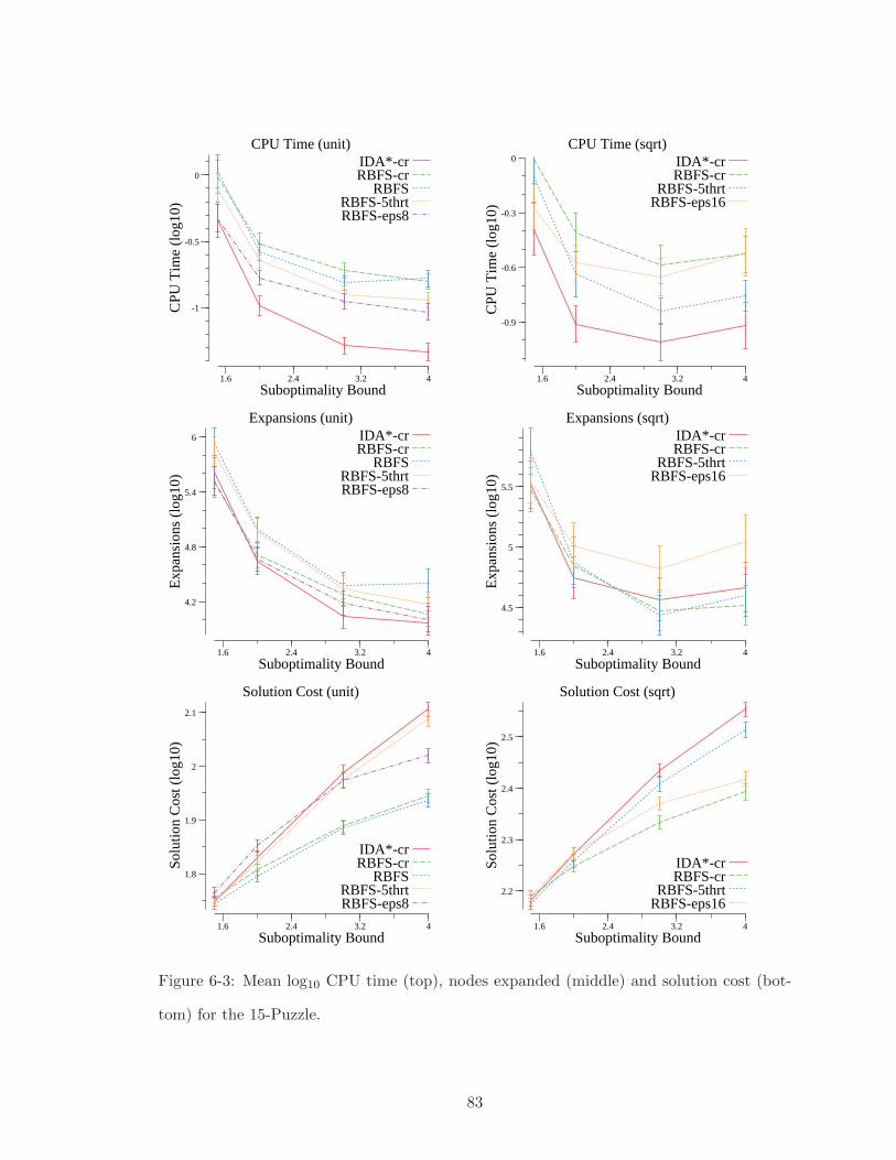
CPU Time (unit)

Suboptimality Bound1.6 2.4 3.2 4

CPU

Tim

e (l

og10

)

-1

-0.5

0IDA*-crRBFS-cr

RBFSRBFS-5thrtRBFS-eps8

CPU Time (sqrt)

Suboptimality Bound1.6 2.4 3.2 4

CPU

Tim

e (l

og10

)

-0.9

-0.6

-0.3

0 IDA*-crRBFS-cr

RBFS-5thrtRBFS-eps16

Expansions (unit)

Suboptimality Bound1.6 2.4 3.2 4

Exp

ansi

ons

(log

10)

4.2

4.8

5.4

6 IDA*-crRBFS-cr

RBFSRBFS-5thrtRBFS-eps8

Expansions (sqrt)

Suboptimality Bound1.6 2.4 3.2 4

Exp

ansi

ons

(log

10)

4.5

5

5.5

IDA*-crRBFS-cr

RBFS-5thrtRBFS-eps16

Solution Cost (unit)

Suboptimality Bound1.6 2.4 3.2 4

Solu

tion

Cos

t (lo

g10)

1.8

1.9

2

2.1

IDA*-crRBFS-cr

RBFSRBFS-5thrtRBFS-eps8

Solution Cost (sqrt)

Suboptimality Bound1.6 2.4 3.2 4

Solu

tion

Cos

t (lo

g10)

2.2

2.3

2.4

2.5

IDA*-crRBFS-cr

RBFS-5thrtRBFS-eps16

Figure 6-3: Mean log10 CPU time (top), nodes expanded (middle) and solution cost (bot-

tom) for the 15-Puzzle.

83

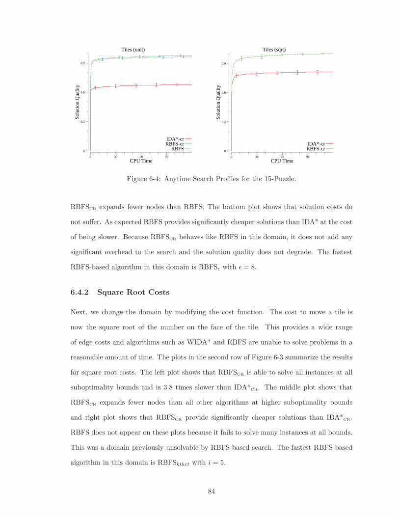
Tiles (unit)

CPU Time0 30 60 90

Solu

tion

Qua

lity

0

0.3

0.6

0.9

IDA*-crRBFS-cr

RBFS

Tiles (sqrt)

CPU Time0 30 60 90

Solu

tion

Qua

lity

0

0.3

0.6

0.9

IDA*-crRBFS-cr

Figure 6-4: Anytime Search Profiles for the 15-Puzzle.

RBFSCR expands fewer nodes than RBFS. The bottom plot shows that solution costs do

not suffer. As expected RBFS provides significantly cheaper solutions than IDA* at the cost

of being slower. Because RBFSCR behaves like RBFS in this domain, it does not add any

significant overhead to the search and the solution quality does not degrade. The fastest

RBFS-based algorithm in this domain is RBFSǫ with ǫ = 8.

6.4.2 Square Root Costs

Next, we change the domain by modifying the cost function. The cost to move a tile is

now the square root of the number on the face of the tile. This provides a wide range

of edge costs and algorithms such as WIDA* and RBFS are unable to solve problems in a

reasonable amount of time. The plots in the second row of Figure 6-3 summarize the results

for square root costs. The left plot shows that RBFSCR is able to solve all instances at all

suboptimality bounds and is 3.8 times slower than IDA*CR. The middle plot shows that

RBFSCR expands fewer nodes than all other algorithms at higher suboptimality bounds

and right plot shows that RBFSCR provide significantly cheaper solutions than IDA*CR.

RBFS does not appear on these plots because it fails to solve many instances at all bounds.

This was a domain previously unsolvable by RBFS-based search. The fastest RBFS-based

algorithm in this domain is RBFSkthrt with i = 5.

84

6.4.3 Anytime Heuristic Search

Hansen and Zhou (2007) propose a simple method for converting a suboptimal heuristic

search into an anytime algorithm: simply continue searching after finding the first solution.

We compared the anytime profiles of RBFS, RBFSCR and IDA*CR. Each algorithm was

given a total of 2 minutes to find and improve a solution. We used the same Korf 100

15-Puzzle instances with unit and square root cost. In Figure 6-4 the x-axis is CPU time

and the y-axis is solution quality. Each data point is computed in a paired manner by

determining the best solution found on each instance by any algorithm and dividing this

value by the incumbent solution’s cost at each time value on the same instance (Coles,

Coles, Olaya, Jimenez, Lopez, Sanner, & Yoon, 2012). Incumbents are initialized to infinity

which allows for comparisons between algorithms at times before all instances are solved.

The lines show the mean over the instance set and the error bars show the 95% confidence

interval on the mean.

The left plot in Figure 6-4 summarizes the results for unit costs. The initial subopti-

mality bound of 4.0 was selected to minimize time to first solution for all algorithms. RBFS

and RBFSCR both are able to find solutions as quickly as IDA*CR but with better solution

quality. The RBFS-based algorithms are able to find the highest quality solutions (above

0.9) while IDA*CR is not able to improve the solution quality beyond 0.7. The right plot

in Figure 6-4 summarizes the results for sqrt costs. Again, an initial suboptimality bound

of 3.0 was selected to minimize the time for first solution for all algorithms. This plot is

similar to the previous one with the exception that RBFS is omitted since it was not able to

solve many instances at any suboptimality bound. Again RBFSCR is able to find solutions

quickly and of better quality than that of IDA*CR. The best-first order of RBFS-based

algorithms proves to be a significant advantage in an anytime setting.

85

6.5 Discussion

IDA* and IDA*CR are high performing algorithms. They benefit from optimizations such

as in-place node expansion and, unlike RBFSCR, they do not require any sorting or sophis-

ticated data structures. Because of this it is difficult to surpass their run-time performance

on the domains tested. However, RBFS-based algorithms use a best-first search order. As

the suboptimality bound loosens RBFS expands significantly fewer nodes while the solution

costs returned remain relatively stable. RBFSCR extends RBFS to domains that it could not

solve previously without sacrificing solution costs. Our results show that RBFSCR expands

roughly the same number of nodes or fewer than IDA*. Furthermore, our implementations

of IDA* and IDA*CR were highly optimized while RBFSCR was not. It is possible that

a more efficient implementation could challenge IDA*, especially for domains where node

expansions are expensive eg., domains where heuristics are expensive to compute.

6.6 Conclusion

We presented three techniques for controlling the overhead caused by excessive backtrack-

ing in RBFS. We showed that two simple techniques, RBFSǫ and RBFSkthrt, work well

in practice, although they do not provide provable guarantees on performance. RBFSCR

is a more complex technique that provides provable guarantees of bounded re-expansion

overhead. We show that these new algorithms perform well in practice, finding solutions

faster than RBFS and finding significantly cheaper solutions than WIDA* for the domains

tested. RBFSCR is the first linear space best-first search capable of solving problems with

a wide variety of f values. While IDA* enjoys widespread popularity, this work indicates

that it may be time for a re-assessment of RBFS.

86

CHAPTER 7

BOUNDED SUBOPTIMAL SEARCH IN LINEAR SPACE

7.1 Introduction

While bounded suboptimal search algorithms scale to problems that A* cannot solve, for

large problems or tight suboptimality bounds, they can still overrun memory. It is possible

to combine linear-space search with bounded suboptimal search to solve problems that can-

not be solved by either method alone. Unfortunately, because linear-space search algorithms

are based on iterative deepening depth-first search they are not able to incorporate distance-

to-go estimates directly. The first contribution of this chapter demonstrates how solution

length estimates provide an alternative to distance-to-go estimates that can be exploited

in bounded suboptimal search. In an empirical analysis we show that solution length esti-

mates can significantly improve the performance of A∗

ǫ and, to a lesser degree, EES. Next,

we demonstrate that solution length estimates allow, for the first time, linear-space variants

of these algorithms. The second contribution is new linear-space variants of A∗

ǫ and EES

based on IDA*: Iterative Deepening A∗

ǫ (IDA∗

ǫ ) and Iterative Deepening EES (IDEES).

These algorithms achieve a new state-of-the-art in linear-space bounded suboptimal search,

surpassing WIDA*.

Unlike WA* and EES, which converge to greedy search as the suboptimality bound

approaches infinity, WIDA*, IDA∗

ǫ and IDEES behave like depth-first search, resulting in

more costly solutions and in some cases, longer solving times than WA*. Recursive Best-

First Search (RBFS, Korf, 1993) on the other hand, is a much better linear space analog

of WA*. It uses the same best-first search order of WA* and converges to greedy search

and returns cheaper solutions. The third contribution of this chapter is new linear space

analogs for A∗

ǫ and EES based on RBFS: Recursive Best-First A∗

ǫ (RBA∗

ǫ ) and Recursive

87

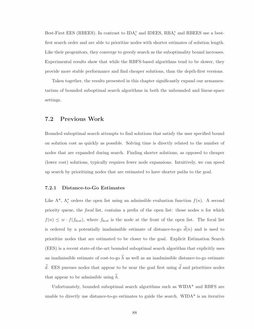
Best-First EES (RBEES). In contrast to IDA∗

ǫ and IDEES, RBA∗

ǫ and RBEES use a best-

first search order and are able to prioritize nodes with shorter estimates of solution length.

Like their progenitors, they converge to greedy search as the suboptimality bound increases.

Experimental results show that while the RBFS-based algorithms tend to be slower, they

provide more stable performance and find cheaper solutions, than the depth-first versions.

Taken together, the results presented in this chapter significantly expand our armamen-

tarium of bounded suboptimal search algorithms in both the unbounded and linear-space

settings.

7.2 Previous Work

Bounded suboptimal search attempts to find solutions that satisfy the user specified bound

on solution cost as quickly as possible. Solving time is directly related to the number of

nodes that are expanded during search. Finding shorter solutions, as opposed to cheaper

(lower cost) solutions, typically requires fewer node expansions. Intuitively, we can speed

up search by prioritizing nodes that are estimated to have shorter paths to the goal.

7.2.1 Distance-to-Go Estimates

Like A*, A∗

ǫ orders the open list using an admissible evaluation function f(n). A second

priority queue, the focal list, contains a prefix of the open list: those nodes n for which

f(n) ≤ w · f(fbest), where fbest is the node at the front of the open list. The focal list

is ordered by a potentially inadmissible estimate of distance-to-go d(n) and is used to

prioritize nodes that are estimated to be closer to the goal. Explicit Estimation Search

(EES) is a recent state-of-the-art bounded suboptimal search algorithm that explicitly uses

an inadmissible estimate of cost-to-go h as well as an inadmissible distance-to-go estimate

d. EES pursues nodes that appear to be near the goal first using d and prioritizes nodes

that appear to be admissible using h.

Unfortunately, bounded suboptimal search algorithms such as WIDA* and RBFS are

unable to directly use distance-to-go estimates to guide the search. WIDA* is an iterative

88

deepening depth-first search using an upper bound on solution cost to prune parts of the

search space. WIDA* increases the upper bound at each iteration to explore deeper parts of

the search tree. It is not possible to perform iterative deepening using just a distance-to-go

estimate since this estimate will tend to decrease along a path. RBFS, on the other hand,

uses a virtual frontier ordered by increasing f to perform a best-first search. One could

imagine incorporating distance-to-go estimates by ordering the frontier by increasing d.

Unfortunately this results in poor performance because of excessive backtracking overhead.

We now turn our attention to how solution length estimates provide an alternative that

can be exploited in bounded suboptimal search.

7.3 Using Solution Length Estimates

Intuitively, A∗

ǫ can be viewed as an algorithm that is doing a Speedy search (a greedy

search on d) with an adaptive upper bound on solution cost. Nodes that are estimated

to be closer to a goal are expanded first. These nodes also tend to be the nodes with the

highest estimate of solution cost f and are more likely to lead to inadmissible solutions,

resulting in the thrashing behavior that is often observed in A∗

ǫ . EES explicitly tries to avoid

inadmissible solutions by using f to shape the focal list. However, if f does not compensate

enough for the error in f , then it is possible even for EES to be lead down unfruitful paths.

Intuitively, shorter paths will tend to be cheaper and more likely to lead to admissible

solutions. By prioritizing nodes that are estimated to have shorter overall solution length

rather than just least distance-to-go we can achieve faster search by avoiding many paths

that are estimated to lead to inadmissible solutions.

We can view Speedy search as a special case of a weighted search using solution length.

We define the solution length estimate of a node n as follows:

l′(n) = (1−Wd) · depth(n) +Wd · d(n)

As the value for Wd increases, the search acts more like Speedy search, converging to

Speedy search as Wd approaches 1. The evaluation function used to order the focal list

89

Sliding Tiles Inverse Tiles Vacuum World

Total

CPU

Tim

eLog

10

Suboptimality Bound5432

2.4

1.6

A*ep

A*ep_l

EES

EES_l

Suboptimality Bound84

2.4

1.6

EES

A*ep

EES_l

A*ep_l

Suboptimality Bound432

2.4

1.6

A*ep

A*ep_l

EES_l

EES

Figure 7-1: Total CPU time (in log10) for A∗

ǫ and EES using estimates of total solution

length vs. estimates of distance-to-go.

in the original EES and A∗

ǫ is a special case of l′ with Wd = 1. As we will see in the

experiments, we can improve the search behavior of A∗

ǫ and EES by having a non-zero

weight on the depth component, thus informing these algorithms of the depth of potential

solutions. Paths that are estimated to be long will fall to the back of the focal list and

paths that are estimated to be shorter will be expanded first.

7.3.1 Empirical Evaluation

To determine the effectiveness of using solution length estimates, we implemented A∗

ǫ and

EES and compared them using solution length and distance-to-go estimates. For all ex-

periments we used path-based single step error correction of the admissible heuristic h to

construct a more accurate but potentially inadmissible heuristic h, as described by Thayer

and Ruml (2010). For our solution length estimates, we used the same value used by the

upper bound on solution cost W to set the value for Wd. All algorithms were written in

Java using the optimizations suggested by Hatem et al. (2013) and compiled with OpenJDK

1.6.0.24. All of our experiments were run on a machine with a CoreDuo 3.16 GHz processor

and 8 GB of RAM running Linux.

90

7.3.2 15-Puzzle

We first consider a simple unit-cost domain: Korf’s 100 15-puzzles. We used the Manhattan

distance heuristic for both heuristic and distance-to-go estimates. The first plot of Figure 7-

1 summarizes the results for unit cost 15-puzzle. This plot shows the total CPU time in log10

for solving all 100 instances. Algorithms that use solution length estimates have suffix of l.

This plot shows that A∗

ǫ is significantly faster using solution length estimates, especially at

lower suboptimality bounds. A∗

ǫ cannot even solve all instances with suboptimality bounds

less than 2 when using just distance-to-go estimates because it exceeds the limit of 8 GB of

available memory. EES using length estimates is the fastest algorithm overall and is faster

than EES using distance-to-go estimates, however the improvement is small compared to

the difference observed in A∗

ǫ . This may be explained by considering solution length to be

a proxy for f . Since EES is already guided by f , the additional guidance from solution

length is not as beneficial.

Next, we change the domain slightly by modifying the cost function. We set the cost

to move a tile to the inverse of the number on the face of the tile. We use the inverse cost

Manhattan distance for the heuristic and a unit cost Manhattan distance for the distance-

to-go estimate. This provides a wide range of edge costs in a simple, well understood

domain. This simple change makes the heuristic less effective in guiding the search, making

the problems harder to solve. Moreover, distance-to-go estimates provide a significant

advantage over using the Manhattan distance heuristic alone. The second plot in Figure 7-

1 summarizes the results for inverse cost 15-puzzle. This plot echos the results seen in

the plot for unit tiles: A∗

ǫ improves significantly with solution length estimates and EES is

slightly faster.

7.3.3 Vacuum World

Next we compared these algorithms on the Vacuum World domain, the first state space

introduced in Russell and Norvig (2003). In this domain a vacuum robot must clean up

dirt distributed across a grid world. In the original description of this problem, each action

91

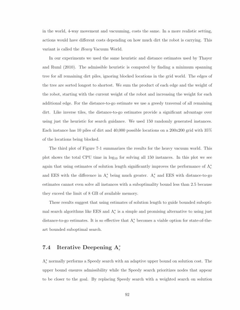
in the world, 4-way movement and vacuuming, costs the same. In a more realistic setting,

actions would have different costs depending on how much dirt the robot is carrying. This

variant is called the Heavy Vacuum World.

In our experiments we used the same heuristic and distance estimates used by Thayer

and Ruml (2010). The admissible heuristic is computed by finding a minimum spanning

tree for all remaining dirt piles, ignoring blocked locations in the grid world. The edges of

the tree are sorted longest to shortest. We sum the product of each edge and the weight of

the robot, starting with the current weight of the robot and increasing the weight for each

additional edge. For the distance-to-go estimate we use a greedy traversal of all remaining

dirt. Like inverse tiles, the distance-to-go estimates provide a significant advantage over

using just the heuristic for search guidance. We used 150 randomly generated instances.

Each instance has 10 piles of dirt and 40,000 possible locations on a 200x200 grid with 35%

of the locations being blocked.

The third plot of Figure 7-1 summarizes the results for the heavy vacuum world. This

plot shows the total CPU time in log10 for solving all 150 instances. In this plot we see

again that using estimates of solution length significantly improves the performance of A∗

ǫ

and EES with the difference in A∗

ǫ being much greater. A∗

ǫ and EES with distance-to-go

estimates cannot even solve all instances with a suboptimality bound less than 2.5 because

they exceed the limit of 8 GB of available memory.

These results suggest that using estimates of solution length to guide bounded subopti-

mal search algorithms like EES and A∗

ǫ is a simple and promising alternative to using just

distance-to-go estimates. It is so effective that A∗

ǫ becomes a viable option for state-of-the-

art bounded suboptimal search.

7.4 Iterative Deepening A∗ǫ

A∗

ǫ normally performs a Speedy search with an adaptive upper bound on solution cost. The

upper bound ensures admissibility while the Speedy search prioritizes nodes that appear

to be closer to the goal. By replacing Speedy search with a weighted search on solution

92

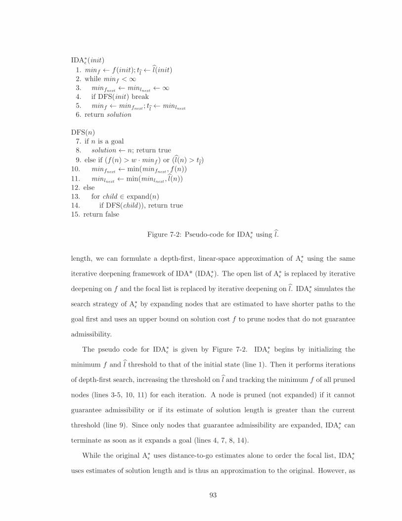
IDA∗

ǫ (init)

1. minf ← f(init); tl← l(init)

2. while minf <∞3. minfnext ← min lnext ←∞4. if DFS(init) break5. minf ← minfnext ; tl ← min lnext

6. return solution

DFS(n)7. if n is a goal8. solution ← n; return true

9. else if (f(n) > w ·minf ) or (l(n) > tl)

10. minfnext ← min(minfnext , f(n))

11. min lnext ← min(min lnext , l(n))12. else13. for child ∈ expand(n)14. if DFS(child)), return true15. return false

Figure 7-2: Pseudo-code for IDA∗

ǫ using l.

length, we can formulate a depth-first, linear-space approximation of A∗

ǫ using the same

iterative deepening framework of IDA* (IDA∗

ǫ ). The open list of A∗

ǫ is replaced by iterative

deepening on f and the focal list is replaced by iterative deepening on l. IDA∗

ǫ simulates the

search strategy of A∗

ǫ by expanding nodes that are estimated to have shorter paths to the

goal first and uses an upper bound on solution cost f to prune nodes that do not guarantee

admissibility.

The pseudo code for IDA∗

ǫ is given by Figure 7-2. IDA∗

ǫ begins by initializing the

minimum f and l threshold to that of the initial state (line 1). Then it performs iterations

of depth-first search, increasing the threshold on l and tracking the minimum f of all pruned

nodes (lines 3-5, 10, 11) for each iteration. A node is pruned (not expanded) if it cannot

guarantee admissibility or if its estimate of solution length is greater than the current

threshold (line 9). Since only nodes that guarantee admissibility are expanded, IDA∗

ǫ can

terminate as soon as it expands a goal (lines 4, 7, 8, 14).

While the original A∗

ǫ uses distance-to-go estimates alone to order the focal list, IDA∗

ǫ

uses estimates of solution length and is thus an approximation to the original. However, as

93

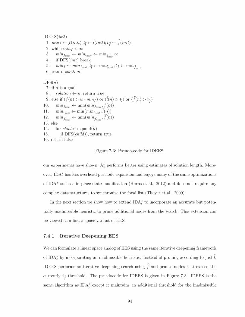
IDEES(init)

1. minf ← f(init); tl← l(init); t

f← f(init)

2. while minf <∞3. minfnext ← min lnext ← min

fnext∞

4. if DFS(init) break5. minf ← minfnext ; tl ← min lnext ; tf ← min

fnext

6. return solution

DFS(n)7. if n is a goal8. solution ← n; return true

9. else if (f(n) > w ·minf ) or (l(n) > tl) or (f(n) > t

f)

10. minfnext ← min(minfnext , f(n))

11. min lnext ← min(min lnext , l(n))

12. minfnext← min(min

fnext, f(n))

13. else14. for child ∈ expand(n)15. if DFS(child)), return true16. return false

Figure 7-3: Pseudo-code for IDEES.

our experiments have shown, A∗

ǫ performs better using estimates of solution length. More-

over, IDA∗

ǫ has less overhead per node expansion and enjoys many of the same optimizations

of IDA* such as in place state modification (Burns et al., 2012) and does not require any

complex data structures to synchronize the focal list (Thayer et al., 2009).

In the next section we show how to extend IDA∗

ǫ to incorporate an accurate but poten-

tially inadmissible heuristic to prune additional nodes from the search. This extension can

be viewed as a linear-space variant of EES.

7.4.1 Iterative Deepening EES

We can formulate a linear space analog of EES using the same iterative deepening framework

of IDA∗

ǫ by incorporating an inadmissible heuristic. Instead of pruning according to just l,

IDEES performs an iterative deepening search using f and prunes nodes that exceed the

currently tfthreshold. The psuedocode for IDEES is given in Figure 7-3. IDEES is the

same algorithm as IDA∗

ǫ except it maintains an additional threshold for the inadmissible

94

heuristic f .

The focal list of EES affords a Speedy search (greedy search on distance-to-go). However,

because IDEES is a depth-first search, it can only approximate the search strategy of EES

by using solution length estimates. This puts IDEES at a disadvantage when there is little

error in distance-to-go estimates. EES can converge to Speedy search sooner than IDEES

in this case. However, when the distance-to-go estimates have high error or if f does not

compensate enough for the error in f , using solution length will provide for a more robust

search strategy.

7.5 Recursive Best-First A∗ǫ and EES

IDA∗

ǫ and IDEES are simpler to implement than their best-first progenitors. However, like

WIDA*, they are both based on depth-first search and, as we will see in our empirical results

below, their performance can degrade as the upper bound loosens. They also return higher

cost solutions on average when compared to best-first algorithms like WA* and RBFS.

RBFS follows the same best-first search order of WA*, resulting in stable performance

and cheaper solutions. This motivates the development of RBFS-based variants of these

algorithms (RBA∗

ǫ and RBEES).

RBA∗

ǫ replaces the depth-first search component of IDA∗

ǫ with recursive depth-first

search. Like IDA∗

ǫ RBA∗

ǫ performs iterative deepening on solution cost estimates f . At

each iteration, RBA∗

ǫ performs a bounded RBFS search, ordering nodes according to so-

lution length estimates and pruning all nodes that exceed the upper bound. RBEES is

similar, except that it incorporates an additional upper bound on solution cost using an

accurate but inadmissible heuristic h. RBEES prunes a node n if it exceeds either upper

bound.

The pseudocode for RBA∗

ǫ and RBEES is given by Figure 7-4, ignoring the code in

square brackets for RBA∗

ǫ . Like IDA∗

ǫ , the search begins by initializing the upper bound

on solution cost to be the estimated solution cost of the initial state (lines 1). The search

proceeds by performing a series of RBFS searches (lines 2, 5, 9-15) expanding nodes in

95

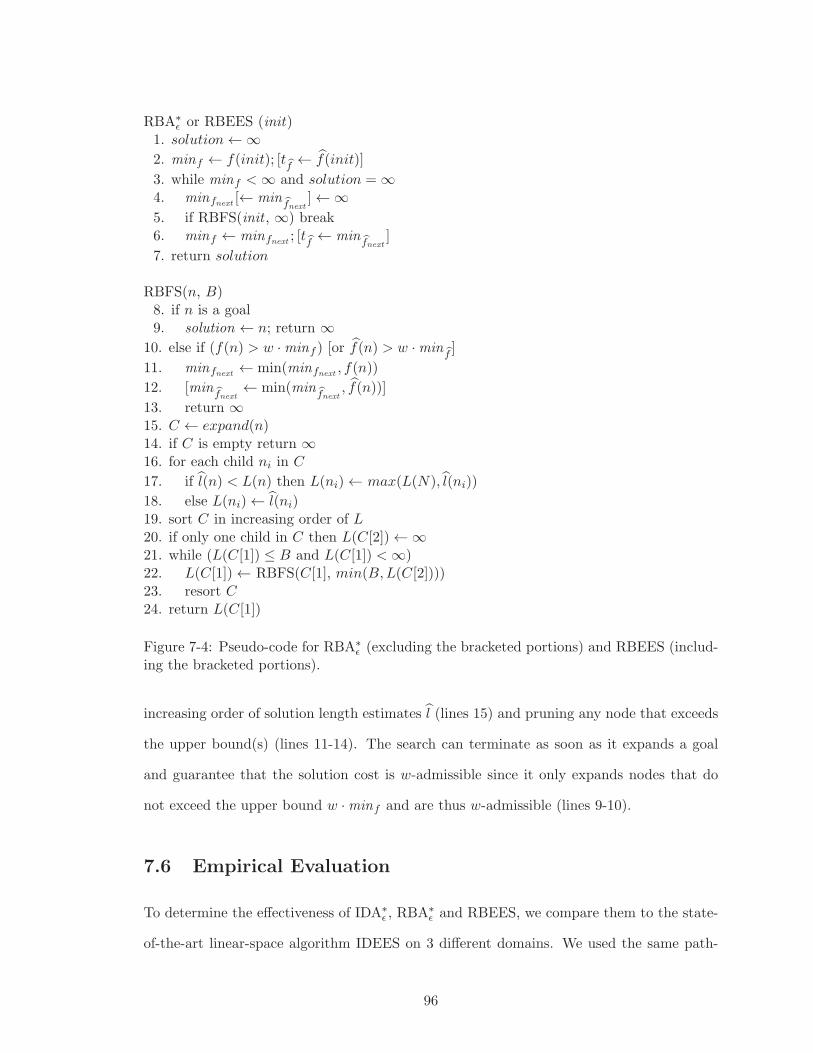
RBA∗

ǫ or RBEES (init)1. solution←∞

2. minf ← f(init); [tf← f(init)]

3. while minf <∞ and solution =∞4. minfnext [← min

fnext]←∞

5. if RBFS(init , ∞) break6. minf ← minfnext ; [tf ← min

fnext]

7. return solution

RBFS(n, B)8. if n is a goal9. solution ← n; return ∞

10. else if (f(n) > w ·minf ) [or f(n) > w ·minf]

11. minfnext ← min(minfnext , f(n))

12. [minfnext← min(min

fnext, f(n))]

13. return ∞15. C ← expand(n)14. if C is empty return ∞16. for each child ni in C

17. if l(n) < L(n) then L(ni)← max(L(N), l(ni))

18. else L(ni)← l(ni)19. sort C in increasing order of L20. if only one child in C then L(C[2])←∞21. while (L(C[1]) ≤ B and L(C[1]) <∞)22. L(C[1])← RBFS(C[1], min(B,L(C[2])))23. resort C24. return L(C[1])

Figure 7-4: Pseudo-code for RBA∗

ǫ (excluding the bracketed portions) and RBEES (includ-ing the bracketed portions).

increasing order of solution length estimates l (lines 15) and pruning any node that exceeds

the upper bound(s) (lines 11-14). The search can terminate as soon as it expands a goal

and guarantee that the solution cost is w-admissible since it only expands nodes that do

not exceed the upper bound w ·minf and are thus w-admissible (lines 9-10).

7.6 Empirical Evaluation

To determine the effectiveness of IDA∗

ǫ , RBA∗

ǫ and RBEES, we compare them to the state-

of-the-art linear-space algorithm IDEES on 3 different domains. We used the same path-

96

based single step error correction to construct h, and the same machines and limits as in

the previous experiments.

7.6.1 15-Puzzle

The first column in Figure 7-5 summarizes the results for unit tiles. The top plot shows the

total CPU time for solving all 100 instances. In this plot we see that both RBA∗

ǫ and RBEES

improve on the performance of WRBFS and perform about the same with bounds greater

than 2. RBA∗

ǫ is not able to solve all instances with smaller bounds. IDEES is slightly

faster and IDA∗

ǫ is the fastest algorithm overall. The bottom plot in the first column shows

the sum of solution costs for all 100 instances. In this plot we see that RBA∗

ǫ and RBEES

return significantly cheaper solutions as the suboptimality bound loosens. As expected,

the RBFS-based algorithms are slower but, like RBFS, they return better solutions than

depth-first algorithms.

Next, we change the domain slightly by modifying the costs to be the sqrt of the number

on the face of the tile. This provides a wide range of edge costs in a simple, well understood

domain. However, the heuristic remains nearly as effective as with unit costs. The second

column in Figure 7-5 summarizes the results for sqrt tiles. These plots echo the same results

from unit tiles: the RBFS-based algorithms are slower overall but provide significantly

cheaper solutions. In this domain WRBFS was not able to solve all instances at any of the

suboptimality bounds. The wide range of f values results in excessive node re-expansion

overhead. RBEES and RBA∗

ǫ are guided by d which has a much narrower distribution.

Next, we compared our algorithms using the inverse cost function. The third column in

Figure 7-6 summarizes the results for inverse tiles. In this domain the heuristic is much less

effective. The RBFS-based algorithms are only able to solve all instances at suboptimality

bounds of 3 or larger. The depth-first search algorithms are much faster but again we see

that for the cases where the RBFS-based algorithms could solve all instances, they return

significantly cheaper solutions.

97

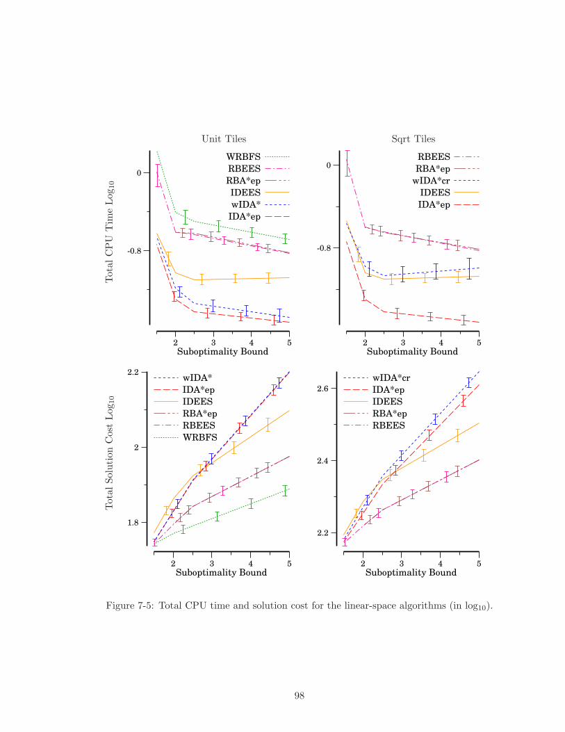
Unit Tiles Sqrt Tiles

Total

CPU

Tim

eLog

10

Suboptimality Bound5432

0

-0.8

WRBFS

RBEES

RBA*ep

IDEES

wIDA*

IDA*ep

Suboptimality Bound5432

0

-0.8

RBEES

RBA*ep

wIDA*cr

IDEES

IDA*ep

Total

Solution

CostLog

10

Suboptimality Bound5432

2.2

2

1.8

wIDA*

IDA*ep

IDEES

RBA*ep

RBEES

WRBFS

Suboptimality Bound5432

2.6

2.4

2.2

wIDA*cr

IDA*ep

IDEES

RBA*ep

RBEES

Figure 7-5: Total CPU time and solution cost for the linear-space algorithms (in log10).

98

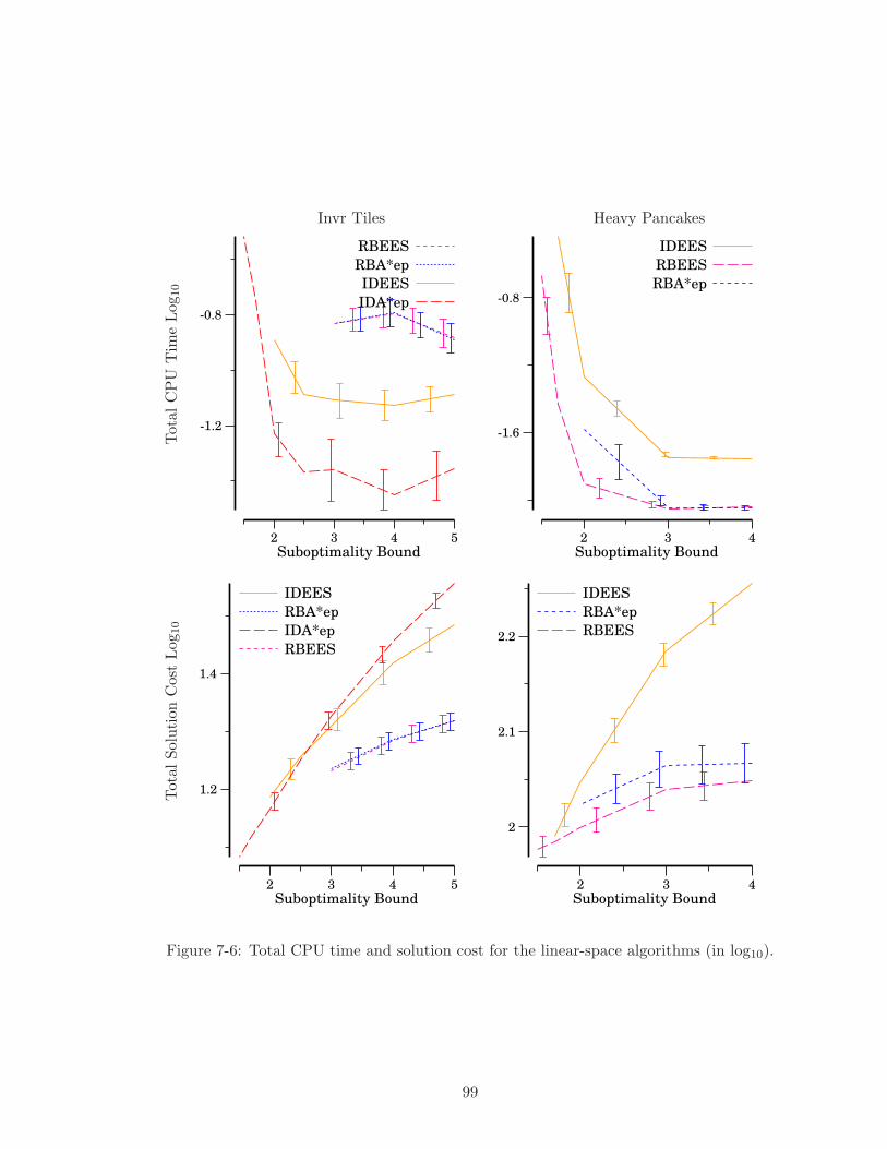
Invr Tiles Heavy Pancakes

Total

CPU

Tim

eLog

10

Suboptimality Bound5432

-0.8

-1.2

RBEES

RBA*ep

IDEES

IDA*ep

Suboptimality Bound432

-0.8

-1.6

IDEES

RBEES

RBA*ep

Total

Solution

CostLog

10

Suboptimality Bound5432

1.4

1.2

IDEES

RBA*ep

IDA*ep

RBEES

Suboptimality Bound432

2.2

2.1

2

IDEES

RBA*ep

RBEES

Figure 7-6: Total CPU time and solution cost for the linear-space algorithms (in log10).

99

7.6.2 Heavy Pancakes

We also evaluated the performance of these algorithms on the heavy pancake puzzle using

the gap heuristic and a stack of 14 pancakes. The last column in Figure 7-6 summarizes

the results for heavy pancakes. In this plot we see that the RBFS-based algorithms are

significantly faster than the depth-first algorithms. Algorithms not shown did not complete

within the timeout and RBA∗

ǫ did not solve instances below a suboptimality bound of 2.

RBA∗

ǫ and RBEES outperform IDEES and provide significantly cheaper solutions.

In summary, these results suggest that, like RBFS, RBA∗

ǫ and RBEES return cheaper

solutions than depth-first-based algorithms, even with non-monotonic cost functions. The

new IDA∗

ǫ variant achieves a new state-of-the-art in the sliding tiles domains and the new

RBEES algorithm surpasses previous work in the heavy pancakes domain.

7.7 Conclusion

In this chapter, we first demonstrated how using estimates of solution length can improve

EES and transform A∗

ǫ into a highly competitive algorithm. We then showed how solution

length estimates enable an iterative deepening depth-first variant of A∗

ǫ and EES. Finally

we presented two new linear-space best-first bounded suboptimal search algorithms, RBA∗

ǫ

and RBEES. Our experiments showed that IDA∗

ǫ achieves a new state-of-the-art in several

domains while the RBFS-based algorithms provide significantly better solution cost as the

bound loosens and also surpass previous work. Taken together, the results presented in this

chapter significantly expand our armamentarium of bounded suboptimal search algorithms

in both the unbounded and linear-space settings.

100

CHAPTER 8

CONCLUSION

This dissertation examined several techniques for scaling heuristic search: the use of external

memory, bounded suboptimal search, and linear-space algorithms. Each chapter addressed

limitations of previous approaches with respect to practically motivated problems. We

have focused on improving scalability of memory efficient heuristic search algorithms by

applying the same techniques used in unbounded space search: best-first search order,

partial expansion, bounded node generation overhead, and distance-to-go estimates. The

new algorithms presented in this dissertation advance the state-of-the-art and make it easier

to apply heuristic search in practical settings.

In chapter 2, we introduced external memory search and focused on the framework of

A*-DDD, something that has been largely overlooked, and showed that an efficient parallel

implementation performs well in practice. We compared A*-DDD with internal memory

search and other previous approaches to external search that forgo best-first search order.

The results of our comparison showed that the best-first search order results in fewer node

generations, saving expensive I/O operations. A*-DDD solves problems faster than both

internal memory search and the alternative external algorithms that forgo a best-first search

order. Unfortunately, A*-DDD does not perform well when the problem exhibits a wide

range of edge costs and large branching factors, two properties often found in real-world

problems that motivate chapters 3 and 4.

In chapter 3, we examined the issue of non-uniform edge costs in more detail and pre-

sented PEDAL, a new parallel external-memory search, that extends the A*-DDD frame-

work to domains with arbitrary edge costs. PEDAL uses a technique inspired by IDA*CR

and using a best-first search order. We proved that a simple layering scheme allows PEDAL

101

to guarantee constant I/O overhead. In addition, we showed empirically that PEDAL gives

very good performance in practice, surpassing serial IDA* on the sliding tiles puzzle, and

nearly equal performance to a parallel IDA*. PEDAL also solves problems more quickly

than existing methods on practically motivated problems with real costs, such as the Dock-

yard Worker planning domain. The results presented in this chapter support our claim that

external search can benefit from a best-first search order and that best-first heuristic search

can scale to large problems that have arbitrary edge costs.

We completed our study of external memory search in chapter 4 where we presented

PE2A*, an extension of PEDAL that combines the partial expansion technique of PEA*

with hash-based delayed duplicate detection to deal with problems that have large branching

factors. Partial expansions significantly reduce the number of expensive I/O operations

making a best-first search feasible. Like PEDAL, PE2A* generates significantly fewer nodes

than IDDP, an alternative external algorithm that forgoes a best-first search order. In

our experiments, PE2A* outperformed serial internal memory search and IDDP and was

the only algorithm capable of solving the most difficult instances of the Reference Set 1

BaliBASE benchmark, achieving a new state-of-the-art for the problem of MSA. These

results provide further evidence to support our claim that a best-first search order should

not be overlooked for optimal search on disk.

In the remaining chapters we examined alternative techniques for reducing the time

and space complexity of heuristic search. In chapter 5, we introduced bounded suboptimal

search and presented simplified variants of A∗

ǫ (SA∗

ǫ ) and EES (SEES) that simplify state-of-

the-art techniques by combining iterative-deepening with bounded suboptimal search. This

approach significantly reduces search overhead by eliminating the need for synchronizing

multiple priority queues. Synchronizing multiple queues requires complex data structures

such as red-black trees for efficiency, and can be difficult to implement. Moreover, even with

these data structures A∗

ǫ and EES still have high overhead compared to simpler algorithms

that use a single priority queue. In an empirical evaluation, we showed that SA∗

ǫ and SEES,

like the originals, outperform other bounded suboptimal search algorithms, such as WA*

102

and confirmed that, while SA∗

ǫ and SEES expand roughly the same number of nodes as

the originals, they solve problems significantly faster, setting a new state-of-the-art in our

benchmark domains. This work introduces ideas that are exploited later in chapter 7 and

provides a general approach that may be applicable to other complex multi-queue based

search algorithms.

Next we examined heuristic search algorithms with linear space complexity. Like ex-

ternal search, linear-space algorithms also make assumptions about the properties of the

search space that are not exhibited by problems with practical relevance. Such problems

often exhibit a wide range of f values. RBFS, the only best-first linear-space search algo-

rithm for non-monotonic cost functions, fails on these problems. In chapter 6, we addressed

this issue with three new techniques for controlling the overhead caused by excessive back-

tracking in RBFS. We showed that two simple techniques, RBFSǫ and RBFSithrt, work well

in practice, although they do not provide provable guarantees on performance. RBFSCR, a

more complex technique, provides provable guarantees of bounded re-expansion overhead.

We showed that these new algorithms perform well in practice, finding solutions faster

than RBFS and finding significantly cheaper solutions than WIDA* for the domains tested.

RBFSCR is the first linear space best-first search capable of solving problems with a wide

variety of f values. While IDA* enjoys widespread popularity, the results presented in this

chapter suggest that it may be time for a re-assessment of RBFS.

Finally, we combined ideas from the previous chapters to make heuristic search even

more scalable on practical domains. In chapter 7, we demonstrated that using estimates of

solution length can improve EES and transform A∗

ǫ into a highly competitive algorithm. We

then showed how solution length estimates enable an iterative deepening depth-first variant

of A∗

ǫ and EES. We also presented two new linear-space best-first bounded suboptimal

search algorithms, RBA∗

ǫ and RBEES. Our experiments showed that IDA∗

ǫ achieves a new

state-of-the-art in several domains while the RBFS-based algorithms provide significantly

better solution cost as the bound loosens and also surpass previous work. Taken together,

the results presented in this chapter significantly expand our armamentarium of bounded

103

suboptimal search algorithms in both the unbounded and linear-space settings.

This dissertation has examined the limitations of previous approaches for scaling heuris-

tic search with respect to real-world problems, such as Multiple Sequence Alignment, that

exhibit properties not typical of toy domains. In each chapter we introduced new techniques

that advance the state-of-the-art and make it easier to apply heuristic search to challenging

problems with practical relevance. While we have stressed the benefits of a best-first search

order, we acknowledge that the algorithms presented herein are not always the algorithms

of choice. For example, a breadth-first search order can provide a significant advantage for

the problem of model checking (Burns & Zhou, 2012). For real-world problems suited to

heuristic search, we intend for this dissertation to act as a guide to maximize performance

and simplify deployment. We are excited by the prospect of applying our techniques to

advance the state-of-the-art for other practically motivated problems such as learning opti-

mal Bayesian networks (Yuan, Malone, & Wu, 2011) and parsing of natural language text

(Klein & Manning, 2003).

104

Bibliography

Altschul, S. F. (1989). Gap costs for multiple sequence alignment. Journal of Theoretical

Biology, 138 (3), 297–309.

Bjornsson, Y., Enzenberger, M., Holte, R. C., & Schaeffer, J. (2005). Fringe search: beating

A* at pathfinding on game maps. In In Proceedings of IEEE Symposium on Compu-

tational Intelligence and Games, pp. 125–132.

Burns, E., Hatem, M., Leighton, M. J., & Ruml, W. (2012). Implementing fast heuristic

search code. In Proceedings of the Symposium on Combinatorial Search (SoCS-12).

Burns, E., & Ruml, W. (2013). Iterative-deepening search with on-line tree size prediction.

Annals of Mathematics and Artificial Intelligence, S68, 1–23.

Burns, E., & Zhou, R. (2012). Parallel model checking using abstraction. In Proceedings of

the Nineteenth International SPIN Workshop on Model Checking of Software (SPIN-

12), pp. 172–190.

Carrillo, H., & Lipman, D. (1988). The multiple sequence alignment problem in biology.

SIAM J. on Applied Mathe- matics, 48 (5), 1073–1082.

Coles, A., Coles, A., Olaya, A. G., Jimenez, S., Lopez, C. L., Sanner, S., & Yoon, S. (2012).

A survey of the seventh international planning competition. AI Magazine, 33 (1),

83–88.

Dayhoff, M. O., Schwartz, R. M., & Orcutt, B. C. (1978). A model of evolutionary change

in proteins. Atlas of protein sequence and structure, 5, 345–351.

Dechter, R., & Pearl, J. (1988). The optimality of A*. In Kanal, L., & Kumar, V. (Eds.),

Search in Artificial Intelligence, pp. 166–199. Springer-Verlag.

Dijkstra, E. (1959). A note on two problems in connexion with graphs. Numerische Math-

ematik, 1 (1), 269–271.

105

Edelkamp, S., Jabbar, S., & Schrdl, S. (2004). External A*. In Advances in Artificial

Intelligence, Vol. 3238, pp. 226–240. Springer Berlin / Heidelberg.

Edelkamp, S., & Kissmann, P. (2007). Externalizing the multiple sequence alignment prob-

lem with affine gap costs. In KI 2007: Advances in Artificial Intelligence, pp. 444–447.

Springer Berlin / Heidelberg.

Felner, A., Goldenberg, M., Sharon, G., Stern, R., Beja, T., Sturtevant, N. R., Schaeffer,

J., & Holte, R. (2012). Partial-Expansion A* with selective node generation. In

Proceedings of AAAI-2012.

Ghallab, M., Nau, D., & Traverso, P. (2004). Automated Planning: Theory and Practice.

Morgan Kaufmann Publishers.

Hansen, E. A., & Zhou, R. (2007). Anytime heuristic search. Journal of Artificial Intelligence

Research, 28, 267–297.

Hart, P. E., Nilsson, N. J., & Raphael, B. (1968). A formal basis for the heuristic determina-

tion of minimum cost paths. IEEE Transactions of Systems Science and Cybernetics,

SSC-4 (2), 100–107.

Hatem, M., Burns, E., & Ruml, W. (2013). Faster problem solving in Java with heuristic

search. IBM DeveloperWorks, 2013.

Helmert, M. (2010). Landmark heuristics for the pancake problem. In Proceedings of the

Symposium on Combinatorial Search (SOCS-10).

Helmert, M., & Roger, G. (2008). How good is almost perfect?. In Proceedings of the

Twenty-Third AAAI Conference on Artificial Intelligence (2008).

Ikeda, T., & Imai, H. (1999). Enhanced A* algorithms for multiple alignments: optimal

alignments for several sequences and k-opt approximate alignments for large cases.

Theoretical Computer Science, 210 (2), 341–374.

Jabbari Arfaee, S., Zilles, S., & Holte, R. C. (2011). Learning heuristic functions for large

state spaces. Artif. Intell., 175 (16-17), 2075–2098.

106

Klein, D., & Manning, C. D. (2003). A* parsing: fast exact Viterbi parse selection. In

Proceedings of the 2003 Conference of the North American Chapter of the Association

for Computational Linguistics on Human Language Technology-Volume 1, pp. 40–47.

Association for Computational Linguistics.

Kobayashi, H., & Imai, H. (1998). Improvement of the A* algorithm for multiple sequence

alignment. In Proceedings of the 9th Workshop on Genome Informatics, pp. 120–130.

Korf, R. (2012). Research challenges in combinatorial search. In Proceedings of AAAI-2012.

Korf, R., & Reid, M. (1998). Complexity analysis of admissibe heuristic search. In Proceed-

ings of the National Conference on Artificial Intelligence, pp. 305–310.

Korf, R. E. (1985a). Depth-first iterative-deepening: An optimal admissible tree search.

Artificial Intelligence, 27 (1), 97–109.

Korf, R. E. (1985b). Iterative-deepening-A*: An optimal admissible tree search. In Pro-

ceedings of the International Joint Conference on Artificial Intelligence (IJCAI-85),

pp. 1034–1036.

Korf, R. E. (1993). Linear-space best-first search. Artificial Intelligence, 62 (1), 41–78.

Korf, R. E. (2003). Delayed duplicate detection: extended abstract. In Proceedings of the

Eighteenth International Joint Conference on Articial Intelligence (IJCAI-03), pp.

1539–1541.

Korf, R. E. (2004). Best-first frontier search with delayed duplicate detection. In Proceedings

of the Nineteenth National Conference on Artificial Intelligence (AAAI-04), pp. 650–

657. AAAI Press.

Korf, R. E. (2008). Linear-time disk-based implicit graph search. Journal of the ACM,

55 (6).

Korf, R. E., Zhang, W., Thayer, I., & Hohwald, H. (2005). Frontier search. Journal of the

ACM, 52 (5), 715–748.

107

Lermen, M., & Reinert, K. (2000). The practical use of the A* algorithm for exact multiple

sequence alignment. Journal of Computational Biology, 7 (5), 655–671.

McCabe, T. (1976). A complexity measure. IEEE Transactions on Software Engineering,

SE-2 (4), 308–320.

Needleman, S. B., & Wunsch, C. D. (1970). A general method applicable to the search for

similarities in the amino acid sequences of two proteins. Journal of Molecular Biology,

48, 443–453.

Niewiadomski, R., Amaral, J. N., & Holte, R. C. (2006). Sequential and parallel algorithms

for Frontier A* with delayed duplicate detection. In Proceedings of AAAI-2006, pp.

1039–1044. AAAI Press.

Pearl, J., & Kim, J. H. (1982). Studies in semi-admissible heuristics. IEEE Transactions

on Pattern Analysis and Machine Intelligence, PAMI-4 (4), 391–399.

Pohl, I. (1973). The avoidance of (relative) catastrophe, heuristic competence, genuine

dynamic weighting and computation issues in heuristic problem solving. In Proceedings

of IJCAI-73, pp. 12–17.

Reinefeld, A., & Schnecke, V. (1994). AIDA* Asynchronous Parallel IDA*. In Proceedings of

the Biennial Conference-Canadian Society for Computational Studies of Intelligence,

pp. 295–302. Canadian Information Processing Society.

Ruml, W., & Do, M. B. (2007). Best-first utility-guided search. In Proceedings of IJCAI-07,

pp. 2378–2384.

Russell, S., & Norvig, P. (2003). Artificial Intelligence: A Modern Approach.

Samadi, M., Felner, A., & Schaeffer, J. (2008). Learning from multiple heuristics. In

Proceedings of AAAI-08.

Sarkar, U., Chakrabarti, P., Ghose, S., & Sarkar, S. D. (1991). Reducing reexpansions in

iterative-deepening search by controlling cutoff bounds. Artificial Intelligence, 50,

207–221.

108

Schroedl, S. (2005). An improved search algorithm for optimal multiple-sequence alignment.

Journal of Artificial Intelligence Research, 23, 587–623.

Thayer, J., & Ruml, W. (2010). Finding acceptable solutions faster using inadmissible

information. Tech. rep. 10-01, University of New Hampshire.

Thayer, J., Ruml, W., & Kreis, J. (2009). Using distance estimates in heuristic search: A

re-evaluation. In Symposium on Combinatorial Search.

Thayer, J. T., Dionne, A., & Ruml, W. (2011). Learning inadmissible heuristics during

search. In Proceedings of ICAPS-11.

Thayer, J. T., & Ruml, W. (2008). Faster than weighted A*: An optimistic approach to

bounded suboptimal search. In Proceedings of the Eighteenth International Conference

on Automated Planning and Scheduling (ICAPS-08).

Thompson, Plewniak, & Poch (1999). BAliBASE: a benchmark alignment database for the

evaluation of multiple alignment programs. Bioinformatics, 15.

Wilt, C. M., & Ruml, W. (2012). When does Weighted A* fail?. In Proceedings of the

Symposium on Combinatorial Search (SoCS-12).

Yoshizumi, T., Miura, T., & Ishida, T. (2000). A* with partial expansion for large branching

factor problems. In Proceedings of AAAI-2000, pp. 923–929.

Yuan, C., Malone, B., & Wu, X. (2011). Learning optimal bayesian networks using A*

search. In Proceedings of the Twenty-Second international joint conference on Artifi-

cial Intelligence-Volume Volume Three, pp. 2186–2191. AAAI Press.

Zhou, R., & Hansen, E. (2009). Dynamic state-space partitioning in external-memory graph

search. In The 2009 International Symposium on Combinatorial Search (SOCS-09).

Zhou, R., & Hansen, E. A. (2003a). Sparse-memory graph search. In IJCAI, pp. 1259–1268.

Zhou, R., & Hansen, E. A. (2003b). Sweep A*: Space-efficient heuristic search in partially

ordered graphs. In Proceedings of the 15th IEEE International Conference on Tools

with Artificial Intelligence (ICTAI-03).

109

Zhou, R., & Hansen, E. A. (2004). Structured duplicate detection in external-memory graph

search. In Proceedings of AAAI-2004.

Zhou, R., & Hansen, E. A. (2006). Breadth-first heuristic search. Artificial Intelligence,

170 (4–5), 385–408.

110