Hierarchical Bayesian Method for the Gravity Equations∗

Meixin Guo†

Department of Economics, School of Economics and Management, Tsinghua University

First draft May 2010; revised August 2010

Abstract

Using panel data on country pairs, there are many ways in which fixed effects maybe included in gravity models to control for countries’ business cycle properties; esti-mates of key parameters can vary considerably, as noted in the literature. This papertries to answer whether the gravity model estimations should include time-varyingor time-invariant dummies, nation or separate importer and exporter dummies, andsymmetric or asymmetric pair dummies. These model selection questions cannot beeasily answered with conventional likelihood ratio tests and Wald tests because thehigh dimensionality of the parameter space due to many fixed effects and hundredsof constraints associated with these hypothesis tests lead to a large size distortion(the type I error). Here the hierarchical Bayesian method is applied to reduce theover-parameterization problem and to help choose models more credibly. This studyestimates the gravity equations for the Euro Zone effect on trade for 22 developedcountries during 1980-2004, a case used previously by Baldwin and Taglioni (2006).The Bayesian results show that the model with time-invariant importer and exporterdummies is preferred.

1 Introduction

Since the 1960s, the gravity equation has been used to explain trade flows between pairs

of countries in terms of the countries’ incomes, distances and other factors. There are four

categories of variables involved in estimation: trade flows, economic mass variables (expen-

ditures, output and income per capita), fixed effects, and paired trade costs.1 Several issues

∗The author is greatly indebted to Paul Bergin, Guido Kuersteiner, and Katheryn Russ for their valuableadvice and constant encouragements, and also very grateful to Colin Cameron and Oscar Jorda for valuablesuggestions. The author also appreciates the comments from macro Brown bag participants at UC Davis.

†Department of Economics, School of Economics and Management, Tsinghua University, Beijing, China,100084. guomx@sem.tsinghua.edu.cn. Phone: 86-10-62795839.

1The trade cost factors have three main categories: a. geography variables, including distance, land-locked and island status, land area, country adjacency, latitude and longitude etc.; b. culture and history

1

are debated in this empirical gravity equation literature, including the choice of dependent

variables and economic mass variables.2

A more severe issue in the gravity estimations is the choice of dummy variables, to include

as fixed effects to control for business cycles and bilateral relations between countries. There

is an increasing debate over how to choose dummies; conclusions on the key parameters vary

with the inclusion of different groups of dummies. The essential questions are whether to

include time-varying or time-invariant dummies, nation or separate importer and exporter

dummies, and symmetric or asymmetric country pair dummies. The model with time-

varying importer and exporter dummies has a theoretical foundation from Anderson and

Van Wincoop (2003) and econometric support in Feenstra and Drive (2002). Evidence of

heterogeneous preferences across countries provides support for the asymmetric pair dummies

as in Guo (2010). These three papers taken together favor a model with both time-varying

importer and exporter dummies, and asymmetric country pair dummies in panel regressions.

However, researchers adopt different specifications of fixed effects in empirical studies.

For example, the two literatures on the WTO and currency union effects show the great-

est disagreements on the choice of dummy variables. Rose (2004) considers time-invariant

country fixed effects and finds little evidence that WTO/GATT promotes the total trade

flow (sum of imports and exports) between a pair of countries. However, Subramanian and

Wei (2007) take into account time-varying importer and exporter fixed effects, and find a

strong positive and asymmetric effect of WTO on bilateral imports across countries and

sectors, increasing world imports around 120% on average.

In the rich literature on currency union effect, Rose and Stanley (2005) evaluate a long list

of estimates using meta regression analysis under two cases: random and fixed effect models.

They find that the positive effect is 47% with a 95% confidence interval of 20%-80%, and

claim that fixed effect estimates provide modest numbers, but suffer biases because of the

heterogeneity. A more recent notable study on Euro Zone effect (EZ) is given by Baldwin

and Taglioni (2006). They find EZ has no significant positive impact on trade controlling

for both time-varying nation and symmetric country pair dummies, in contrast with 58%

in Rose and Van Wincoop (2001) using country fixed effects and 5% - 20% in Micco et al.

(2003) by pair and year dummies. Baldwin and Taglioni (2006) provide great summary and

many comments on the gravity equation literature, but leave open the choice of dummy

variables.

variables, including language, legal system, colony history, current colony status, independence date, devel-opment status etc.; c. special agreement dummies, such as common currency and common regional tradeagreement. See Rose (2004) for details.

2Two main choices have been considered by researchers, trade levels and ratios, including unidirec-tional/total trade flow and imports over countries’ outputs. See appendix A for details.

2

There is no paper in the literature proposing formal empirical criteria to select different

groups of dummy variables. This paper tries to answer the question on choosing dummies to

control for country fixed effects, the multilateral resistance terms in Anderson and Van Win-

coop (2003). The study uses panel data with 22 countries during 1980-2004 (appendix A)

and focuses on the Euro Zone (EZ) and European Union (EU) effects following Baldwin and

Taglioni (2006) and Micco et al. (2003). The variations of these countries (EU vs non-EU,

EZ vs non-EZ) enable discrimination between the EZ and EU effects on trade. I specify

nine models with different choices of dummy variables, which are most commonly used in

the literature, and do the hypothesis testing. The baseline model, one with time-varying

importer and exporter fixed effects and asymmetric country pair fixed effects, is the most

general specification and is implied by the theoretical models. The simplest model only

controls for year and nation fixed effects.

The ordinary panel regressions show that the EZ increases the bilateral import ratio 18%

on average, and the effect varies from a negative 0.3% (insignificant) to 49% (significant) (in

table 5). The Wald test using Newey-West standard errors, the traditional likelihood ratio

test (LR test) and F test based on spherical errors all support the baseline model, where EZ

has no significant effect on imports. However, the LR test and Wald test suffer a really large

size distortion (the type I error) due to the high dimensionality of the parameter space. The

size distortions are also sensitive to the choice of estimates on spherical errors due to the

hundrends of constraints associated with these hypothesis tests. In another words, dimention

adjustment methods change the size distortion in different ways for the LR and Wald tests.

By comparing coefficients and testing hypotheses across models with different fixed ef-

fects, we find symmetric and asymmetric pair fixed effects have a similar influence in estimat-

ing EZ and EU effects. Results also show that individual importer/exporter fixed effects play

a similar role to the nation fixed effects. But the debate on time-varying/time-invariant fixed

effects cannot be resolved by the traditional method. Here the hierarchical Bayesian method

is used to alleviate the small-sample size distortion, to reduce the number of (key) constraints

across models, to estimate the distributions of the fixed effects, and to help select the model

which fits data best. The Bayesian results support the model with time-invariant importer

and exporter fixed effects, where the EZ increases 43% import ratios. With relatively limited

data sets, the different conclusions on the model selection reveals a trade-off between the

small sample problem and omitted variable issue in estimating the high dimenstional gravity

equation.

The structure of the paper is as follows. Section 2 introduces the gravity equation and

different specifications for the dummy variables. Section 3 provides results from least squares

estimation (LS) and maximum likelihood estimation (MLE); and Bayesian results are pre-

3

sented in Section 4. The last section concludes.

2 Euro Effect or European Union Effect?

This section first presents the theoretical gravity model and nine popular empirical spec-

ifications for fixed effects (section 2.1) in the gravity equation literature. The subsequent

subsections provide the results on EZ/EU effects using LS and MLE, and test hypotheses

on different groups of dummy variables.

2.1 Gravity Model

The gravity equation in Anderson and Van Wincoop (2003) augmented with heteroge-

neous preferences in consumption baskets for each country can be shown to yield3

IM ikt =

EXP it

WOUTt

∗ OUT kt

WOUTt

∗WOUTt ∗ αi (k)

(P itΠ

kt

τ ikt

)η−1

(1)

=EXP i

t ∗OUT kt

WOUTt

∗ αi (k)

(P itΠ

kt

τ ikt

)η−1

,

where the multilateral resistance for good k is defined as

(Πk

t

)1−η=

N∑j=1

(P jt

τ jkt

)η−1

αj (k)EXP j

t

WOUTt

,

and the aggregate price level (the multilateral resistance for country i) is defined as

P it =

(N∑k=1

αi (k)[τ ikt Qt (k)

]1−η

) 11−η

.

The gravity equation specifies that the bilateral imports IM ikt are positively influenced

by world output WOUTt, importers’ expenditure shares of world output “EXP it /WOUTt”,

exporters’ output shares of world output “OUT kt /WOUTt”, and preference on good k “αik”,

but are impeded by trade costs “τ ikt ”.4 The choice of dummy variables enters in the spec-

ification of two “multilateral (gravitational inconstant) trade resistance terms” (MLR), i.e.

MLR = (P itΠ

kt )

η−1.

3See section 2 of Guo (2010) for details.4An alternative form of the gravity equation can be found in Head and Mayer (2004) to measure access

to markets, and in Jacks et al. (2008) to measure trade costs.

4

The most general regression equation to estimate EZ and EU effects, the baseline model,

is shown below after we take logs on equation (1)

wikt = cons+ EZ + EU + δik + θit + ϕk

t +3∑

j=1

γjtgikj + εikt . (2)

The dependant variable bilateral import ratio is defined as wikt = log(

IM ikt ∗WOUTt

EXP it ∗OUTk

t),5 and

variables δik are asymmetric country pair dummies to capture the preferences αik. Both

time-varying importer and exporter dummies are used to control for the MLR, log(MLR) =

θit + ϕkt .

The form of bilateral trade costs is assumed as follows

(τ ikt)1−η ≡

J

Πj=1

(Gik

j

)γjt. (3)

Taking logs of both sides of the equation obtains the log of trade costs,J∑

j=1

γjtgikj , where

variables gikj (≡ log(Gik

j

)), include logs of bilateral distances (log(dist.)) and six dummies for

border (contig.), common official language (comlang.), land lock status for both exporter and

importer countries (locked im and locked ex), Euro Zone membership (EZ), and European

Union membership (EU). The variable “EZ” is equal to 1 if both countries belong to the

Euro Zone; and the variable “EU” is equal to 1 if the two countries belong to the European

Union.

Tables 1 and 2 list another eight variations of equation (2) based on different assumptions

on MLR, which are all nested in the baseline model. The two tables respectively use two

versions of dependent variables— log of bilateral import level: limikt = log

(IM ik

t

), and log of

bilateral import ratio: wikt = log

(IM ik

t ∗GOUTt

EXP it ∗OUTk

t

). The eight models arise from combinations of

four key assumptions regarding fixed effects. The first assumption is on country pair dum-

mies, excluding asymmetric pair dummies (δik = 0) or imposing symmetric restrictions on

pair dummies (δik = δki) in the regression. The second one assumes the constant multilateral

resistance; for example, the time-invariant fixed effects take the forms log(MLR) = θi + ϕk

or log(MLR) = µt+ θi+ϕk. The third ignores the different roles for importer and exporter,

and contains nation dummies only, such as log(MLR) = θi + θk. Lastly, if the multilateral

resistance is country-pair specific, the model will have log(MLR) = µt + ζ ik and so that

estimated country pair dummies ζ ik is the sum of two parts, i.e. ζ ik = δik + ζ ik.

5See appendix A for another two versions of estimation equations commonly used in the literature.

5

2.2 Standard Panel Regressions on EZ and EU Effects

The annual data for 22 OECD countries during 1980-2004 are collected mainly following

Baldwin and Taglioni (2006) (appendix A). There are 14 countries in EU by year 1995 and

eight non-EU countries. In the EU group, four countries, Denmark, Greece, Sweden, and

United Kingdom did not join in the EZ by year 2000. The EZ and EU effects on trade can be

distinguished by the variation of these countries. All models are given in tables 1 and 2, and

analyses focus on the table 2 using import ratios to avoid potential endogenous economic

mass variables and non-stationary issue (see appendix A). The baseline model includes

time-varying importer and exporter fixed effects, and asymmetric country pair dummies.

Note that the variable ”lyy” in table 1, the product of current GDPs of the importers and

exporters, is collinear with pair dummies and time-varying nation dummy in table 1, and

hence we could not use the estimated coefficient on this variable to judge which estimation

equation is more supported by intuitions and theories as in Baldwin and Taglioni (2006).

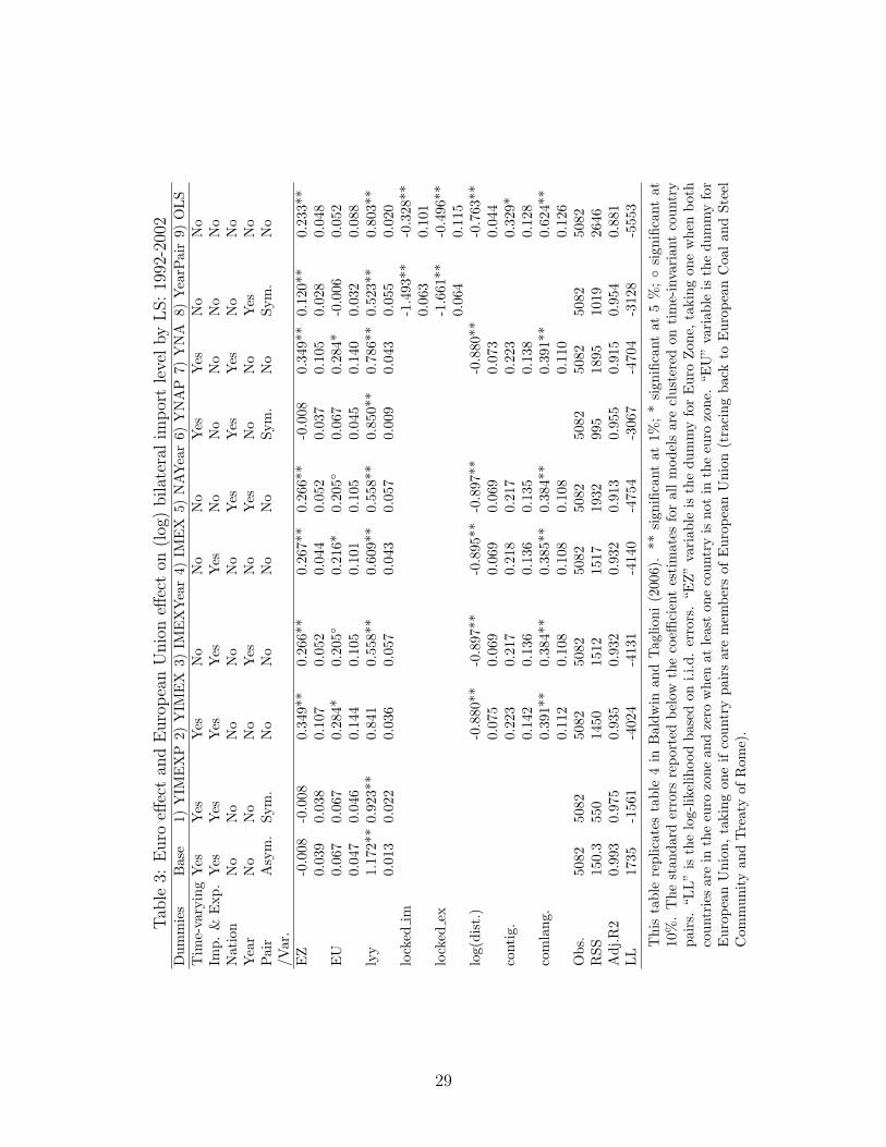
Table 3, using just eleven years of panel data, replicates the key results given in table

4 of Baldwin and Taglioni (2006). The results from the baseline model show that both EZ

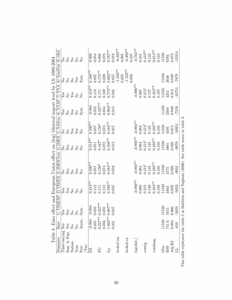
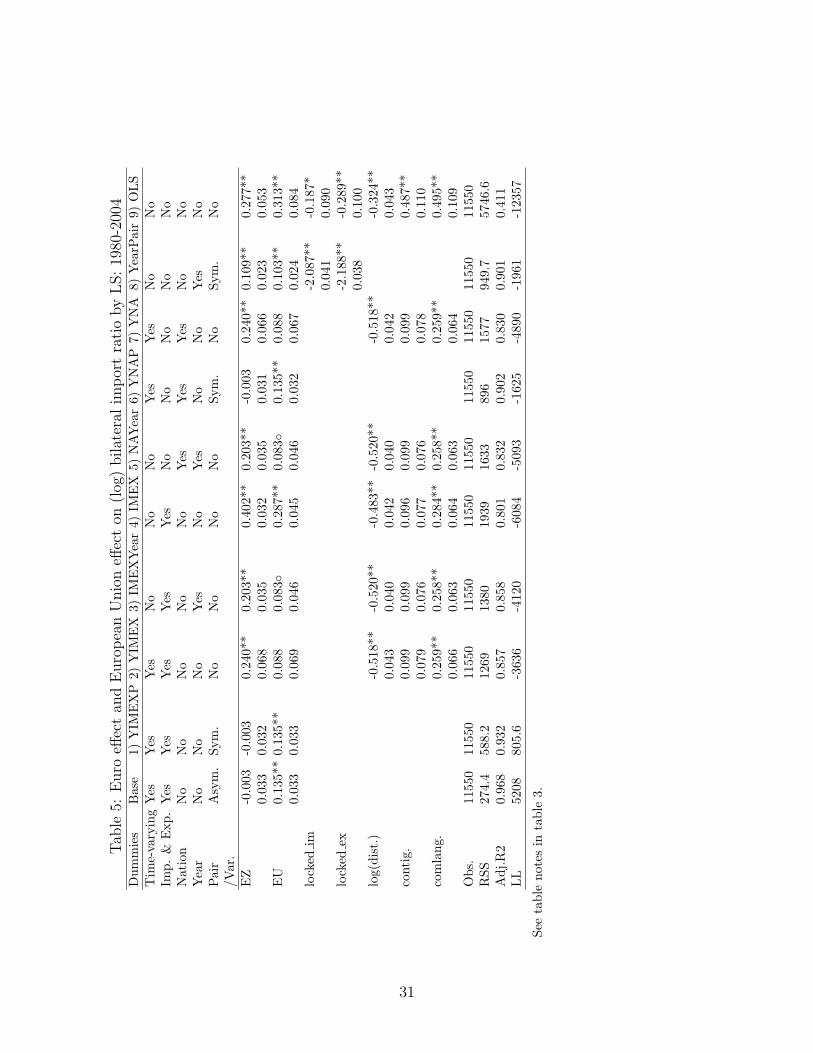
and EU have no significant effect on bilateral imports. Tables 4 and 5 respectively use the

whole 25-year data on import levels and ratios.6 Like in table 3, EZ has no significant effect

on trade in the baseline model of tables 4 and 5 while EU has significant and positive effect

on imports, 25 % for import level in tableolslevel and 14% for import ratios in table 5. The

column “YNAP” with time-varying nation and pair dummies also shows an insignificant EZ

effect on trade, consistent to the result in table 5 of Baldwin and Taglioni (2006). Table 4

for import levels yields qualitatively similar conclusion to table 5. From here on, I focus on

the results for bilateral import ratios to avoid possible endogenous problem.

In table 5, models with symmetric or asymmetric pair dummies and time-varying country

fixed effects (columns of Base, YIMEXP and YNAP) shows that EZ has no significant

effect on imports. However, estimations with time-varying country fixed effects (columns

of YIMEX and YNA) show that using Euros as domestic currency for the trade parterners

can increasethe import ratio by 27%, compared to non-EZ members.7 Estimations with

time-invariant country fixed effects (columns of IMEXYear and NAYear) show that both EZ

and EU have a large effect in promoting import, 23% and 9% respectively. The average EZ

6The trade cost variables are redundant because of multi-collearity with the asymmetric country pairdummies; time-varying importer and exporter dummies also drop one for each country due to the samereason. In this paper with 22-country and 25-year panel data, the base line model drops total 72 dummies,including, 3 trade costs variables, 25 time-varying importer dummies for USA (θUSA

t ), 1 time-varying exporterdummy in 2004 for USA, and another 43 asymmetric country pair dummies.

7The number 27% is equal to e(0.24) − 1 due to the logs. So do other percentages calculated based onthe estimated coefficients.

6

effect increasing import ratios is 18% based on the 11 models and has a range from -0.3% to

49%. The EU effect on import is more stable compared to EZ effect, and varies from 9% to

37% (16% on average). These results illustrate that the EZ and EU effects vary prominantly

with the choice of fixed effects though the standard errors for EZ and EU are similar across

different specifications.

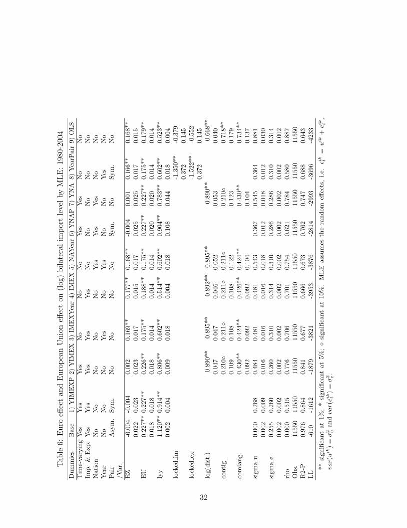
Compared with the above LS results, tables 6 and 7 provide results estimated by MLE for

bilateral import levels and ratios, assuming i.i.d. normally distributed country pair random

effects. MLE results provide robustness check on the variations of EZ and EU effects with the

choice of fixed effects. On average, the MLE results show EZ effect in increasing import ratio

is 11% in table 7, compared to 18% using LS in table 5. The extent of EZ effects depends

on the choice of time-varying or time-invariant country fixed effects. Estimations with time-

varying fixed effects in columns of Base, YIMEXP, YIMEX, YNAP, and YNA, do not provide

evidence to support the EZ effect, but show significant effect from EU membership (15%

more in import ratios). The YearPair model used in Micco et al. (2003) show a 12% increase

in import ratio because of the EZ effect. In contrast, models with time-invariant country

fixed effects in columns of IMEXYear, IMEX, and NAYear, shows both EZ and EU have

significant effects on imports, around 21% and 25 % respectively. If we use simple difference-

in-difference method (DID) within 14 EU member group with four non-EZ countries and take

year 1999 as the breaking point, estimations with time-invariant country fixed effect show

that using euros can increase 15% import ratios. However, after controlling the time-varying

country fixed effect, the EZ effect drops to 5%.

These results from LS, MLE and DID imply three conclusions in estimating the EZ and

EU effects: 1) the difference between symmetric and asymmetric country pair fixed effect

does not matter so much for this sample; 2) isolating the role of importing or exporting

country yields similar results as using nation fixed effects only; 3) furthermore, the choice on

time-varying or constant fixed effects matters magnificently for the estimations on EZ and

EU effects.

2.3 Hypothesis Tests

Based on estimations in table 5, four hypothesis tests on models with different fixed effects

are given in table 8. The classical LR test results are in the LR1 column while the dimension

adjusted LR test is in the LR2 column suggested by Italianer (1985).8 The LR test and F

8Italianer (1985) finds that the LR test statistic is chi-squared distributed with the correction factorm/N , where N is the number of observation and m is equal to (N − r − 0.5 ∗ dn) with the number ofrestrictions r and the dimension dn of the restricted model (the null hypothesis). See append B.1 and table10 for calculations on LR2.

7

test assumes i.i.d. error terms. The “Wald NW” column takes the heteroskedasticity into

account, provides the Wald statistics using Newey-West standard errors with 2 lags,9 which

are robust to HAC (Newey and West (1987, 1994)). All four tests reject the null hypothesis

in the first eight combinations of the null and alternative models. That is, the baseline model

cannot be rejected. If only considering choices on time-varying and time-invariant importer

and exporter dummies, the null hypothesis— time-invarying importer and exporter fixed

effect in combination (9) is supported by all four tests.

These tests suffer from a size distortion due to many fixed effects, pursued in section 3.

Before considering this weakness, we use an alternative model selection procedure: Bayesian

Information Criterion (BIC)

BIC = −2 ∗ LL (y | Θ) + d ∗ log (N) , (4)

where LL (y | Θ) is the log-likelihood, d is the number of the estimated coefficients for a

model, and N is the number of observations. This criterion puts a large penalty on over-

parameterization and is known to favor smaller models compared to hypothesis tests. BIC

statistics for the eleven models,10 are listed in table 9, based on the LS and MLE results

in tables 5, 4, 7, and 6. In the first two LS columns, the baseline model is supported by

BIC. However, in the next two MLE columns, the model with time-invariant nation and

year dummies is preferred by BIC. These two different results on model selection using BIC

come from different specifications of the error terms. The LS assumes spherical errors only,

whereas the MLE additionally considers the i.i.d. country-pair random effects.

3 Size Distortion

The preceding regressions include a large number of dummy variables, especially for the

baseline model; and the hypothesis tests have hundreds of constraints (the degree of freedom

(DF) for the test, the column of “DF” in table 8). Though the hypothesis tests all support

the baseline model, statistical inference may suffer from a small sample problem due to the

unusually high dimensionality of the parameter space and the impressively large group of

constraints associated with the hypothesis tests. As we know, the statistic from the LR test is

asymptotically chi-square distributed with the number of different parameters in the null and

alternative models (DF), when sample size becomes larger. However, with a large number

of parameters and limited data, Evans and Savin (1982) and Italianer (1985) show that the

9The conclusion remains up to 5-lags.10the eleven models include a simple OLS, model with year dummies only and the nine models in tables

1 and 2.

8

finite sample distribution of the statistic is biased towards the conventional large sample

asymptotic chi-square distribution. Therefore, the critical values for the 5% significant level

should be adjusted. But the LR test uses the reported critical values without corrections on

the high dimensionality.

Monte Carlo simulations with i.i.d errors show a large size distortion for the classical

LR test (the LR1 column with spherical errors) in table 10,11 more than 50% on average

(the type I error, the rate of rejecting the null when the null is true). The Wald test (the

Wald1 column) has a even larger size distortion, 77% on average, using the same consistent

but biased estimated variance as in LR1 column. In contrast, the second Wald test (the

Wald2 column) with consistent and unbiased estimated variance and F tests have normal

size. Particularly, the size for the Wald2 test is around 6.7% with relatively larger number

of the constraints (those null models have smaller dimensions compared to the alternative

models). In other words, with a larger group of constraints, the tests have relative greater

size distortions. We reject the models with time-invariant dummies slightly more often (1.7

% more than 5 %) using Wald2 test, and too often for the LR1 and Wald1. The conclusion

is robust to different dependent variables (level or ratio).

Supplementary detailed information for rejection of the null model is provided in fig-

ure 1, which lists the power curves for four combinations of null and alternative models

(see appendix B.1). For example, the first top graph is for the combination of null model

“YNAP”— symmetric country pair and time-varying nation fixed effects, and the alterna-

tive model “Base” — asymmetric country pair and time-varying importer and exporter fixed

effect. The YNAP model is recommended by Baldwin and Taglioni (2006), which can be

obtained by imposing symmetric conditions on the baseline model. Comparison between the

YNAP and the baseline model is to test the null hypotheses H0 are δik = δki and ϕkt = θkt .

By defining δik (= δik − ζ ik) with ζ ik = ζki, and κkt (= ϕk

t − θkt ), the null hypotheses H0 are

equivalent to test δik = 0 and κkt = 0. Accordingly, the null model is nested in the baseline

model. The more volatile δik and κkt , the more frequently the null model will be rejected.

Provided that group of parameters δik and κkt follow normal distributions with a zero mean

and a common standard deviation σ∆, increasing the σ∆ from zero to 0.1, such as 0.01 each

time, leads to a higher chance of rejection on the null model. As a result, the power curve of

the test is determined by the levels of the σ∆. All four tests in figure 1 achieve almost 100%

rejection on the null models when σ∆ = 0.04.

The size distortions shown in table 10, are also sensitive to the choice of estimated

variances (LR1 vs LR2, and Wald1 vs Wald2). In another words, adjusting dimensions on

the statistics reduces the size distortions magnificently. We take the combination (4), IMEX

11See appendix B.1 for simulation details for columns of LR1, LR2, Wald1, Wald2 and F.

9

vs Base, as an example to illustrate this fact using three figures. Figures 2, 3 and 4 provide

the chi-square densities with degree of freedom (DF) 1448 for three cases (appendix B.1): 1)

figures 2 is the ideal case, drawing 1 million observations from the Chi-square distribution

directly; 2) figures 3 plot the LR1 and LR2 statistics using 1000 simulations; 3) figures 4

plot the Wald1 and Wald2 statistics using 1000 simulations. The solid lines use original

values and dash lines are adjusted by dimensions. The shaded areas in all three figures are

5% rejection regions based on the observed densities and the theoretical critical (CV) for

chi-square distribution with DF 1448 is 1537.639.

With DF 1448, the Chi-squared distribution for LR and Wald tests (figures 3 and 4)

are biased compared to the ideal distribution figure 2, where the means are 1555 and 1665

respectively, much larger than true mean 1448. A small adjustment on the statistics (the

dash densities) reduces the size distortion prominently based on the theoretical CV 1537.639.

For example, in figures 2, a value, such as 1539, in the 5% shaded area under the solid line

is changed into 1342.86 with an adjustment (0.873=11550−1448−0.5∗4811550

); this value is no longer

significant compared with the CV 1537.639. In figure 3, LR1 (the solid line) has a 62.1 %

rejection rate on the null model “IMEX” (the size, probability larger than the CV 1537.7).

However, the size becomes zero using LR2 (10). Similar phenomenon occurs in figure 4 for

Wald tests comparing Wald1 with Wald2. The size is 97.6% in column Wald1, but 6.9%

in column Wald2 after the Wald1 statistics are adjusted by 0.87(=11550−149611550

). The three

graphs support the first two conclusions drawn from table 10: the high demensions in the

models and large number of constraints associated with the hypotheis tests lead to a biased

symptotical chi square distribution/large size distortion; futhermore, size distortions could

be sensitive to dimenstion adjustments, the simple adjustment proposed by Italianer (1985)

does not work well for the LR test.

The third conclusion we can draw from table 10 is that misspecified errors evoke close

to 100% size distortion except the two cases: combinations (9) and (10). Considering het-

eroskedasticity and autocorrelation, we consider three HAC forms in the paper (appendix

B.2) and have qualitatively similar results. We mainly focus on “HAC1”, taking the form as

below,

ϵikt = gik + νikt νik

t = bννikt−1 + µik

t var(gik) = σ2gik var(µik

t ) = σ2µ

There is no contemporaneous correlation across county pairs.12 This parametric assumption

considers the heterogeneous fixed effect in the variance covariance matrix Ξ (= var(ϵ)),

which is a block diagonal matrix with Ωik (462 pairs) for one specific country pair (importer

12Models with contemporaneous correlation across county pairs can be estimated by spacial regression.

10

i and exporter k) and Ωik has the following form,

Ωik = σ2gik

1 1 · · · 1

1 1...

......

... 1 1

1 · · · 1 1

+σ2µ

1− b2ν

1 bν · · · bT−1

ν

bν 1...

......

... 1 bν

bT−1ν · · · bν 1

.

In simulations, the true errors have HAC1; and we consider two cases: considering

HAC (the column HAC1) and no controlling for HAC1 (assuming spherical errors) noted as

HAC1(M). The interesting point is that the combinations (9) and (10) have zero rejection for

four tests, in contrast with almost 100% size distortion for other combinations. This result

seems odd at first glance. However, table 11 provides evidence on the large bias in estimating

the coefficients because of the misspecification on the errors. The country-pair specific vari-

ance structure remarkably influences the estimation on the coefficients, particularly for the

country fixed effects. Without controlling for true HAC, both null and alternative models

cannot estimate the coefficients consistently.

Table 11 and the following three tables present the size of the Wald test on the artificial

coefficients and Wald statistics13 for the estimates over 1000 simulations (see appendix B.3).

The null hypothesis in table 11 is H0 : Bm = B0 for m ∈ a, n, and the Wald statistic is

calculated by following formula

Wald = (Bm −B0) ∗[

var(Bm)

]−1

∗ (Bm −B0). (5)

where var(Bm) = σ2m ∗ (X ′

mXm)−1, σ2

m = RSSm/(N − Km), and m = a/n refers to the

alternative/null model. Then the rejection rates (size) for the test is the frequency of rejection

over 1000 simulations. Beside the previous over-rejection fact in the HAC1(M) columns, table

11 also shows that when the null model has a larger dimension (for example, YIMEXP and

YNAP), the size is relative larger, more than 5%. In particular, table 12 focuses on the EZ

and EU effects and gives a similar conclusion on size disortion due to the misspecified error

structure.

Tables 13 and 14 (for EZ and EU effects only) calculate the Wald statistics for H0 :¯Bm = B0 for m ∈ a, c

Wald = (¯Bm −B0) ∗

[

var(¯Bm)

]−1

∗ ( ¯Bm −B0), (6)

13From here on, we use Wald2 as the Wald test with a normal size.

11

where the variance covariance matrix is

var(¯Bm) =

¯σ2m ∗ (X ′

mXm)−1/1000,

and¯σ2m = RSSm/(N−Km) based on the average sum of squared residuals. The Wald statis-

tic follows chi-squared distribution given degrees of freedom/number of constraints. Both

tables show a more rejection in HAC1(M) columns than HOMO and HAC1 columns since

the regressions in HAC1(M) do not consider the HAC. Particularly, in table 14, Wald statis-

tics for the null H0 models (YIMEX and YNA in HOMO column) with yearly importer and

exporter or nation fixed effects, reject the true (artificial) EZ and EU coefficients, indicating

that high dimensionality with a small sample leads to biased estimates on average. A weird

fact is that the alternative models (the H1 column) perform better than the null model (the

H0 column), and they can estimate consistent EZ and EU effects on average for both HOMO

and HAC1 cases, except the two combinations (9) and (10). In these two combinations (9)

and (10), over-parameterization in the alternative model with time-varying fixed effects (H1:

YIMEX) leads to bias on EZ and EU effects in contrast with the null models with constant

fixed effects (H0: IMEX or IMEXY).

Exercises on the size distortion fairly show models with either asymmetric or symmetric

pair fixed effect (Base and YIMEXP) have similar performance in estimating the EZ and EU

effects, and separating importer fixed effect from the exporter fixed effect or using nation

fixed effect only (IMEXYear vs NAYear; and YNA vs YIMEX) leads to similar results too.

However, the issue on time-varying or time-invariant fixed effects (YIMEXP/YIMEX vs

IMEX, YNA vs NAYear) has not been resolved. We need other method to provide the clues

on the problem.

4 Hierarchical Bayesian Method

Previous estimation results and simulations provide relatively consistent support on sym-

metric pair and nation fixed effects for this specific data sample. But there is no clear-cut

evidence against or for time-varying fixed effects. The Bayesian method can estimate the

distributions of all parameters, including the distributions of the variance across years, which

provides direct visual evidence on the volatility of these fixed effect. The hierarchical struc-

ture has the advantage to reduce the dimension of the key parameter space and number of

constraints to test different models, so that alleviate the large dimensionality problem in LS

and MLE. Section 4.1 provides the hierarchical Bayesian model and estimation methodology;

and the next section shows the Bayesian results on model selection.

12

4.1 Estimation Models and Priors

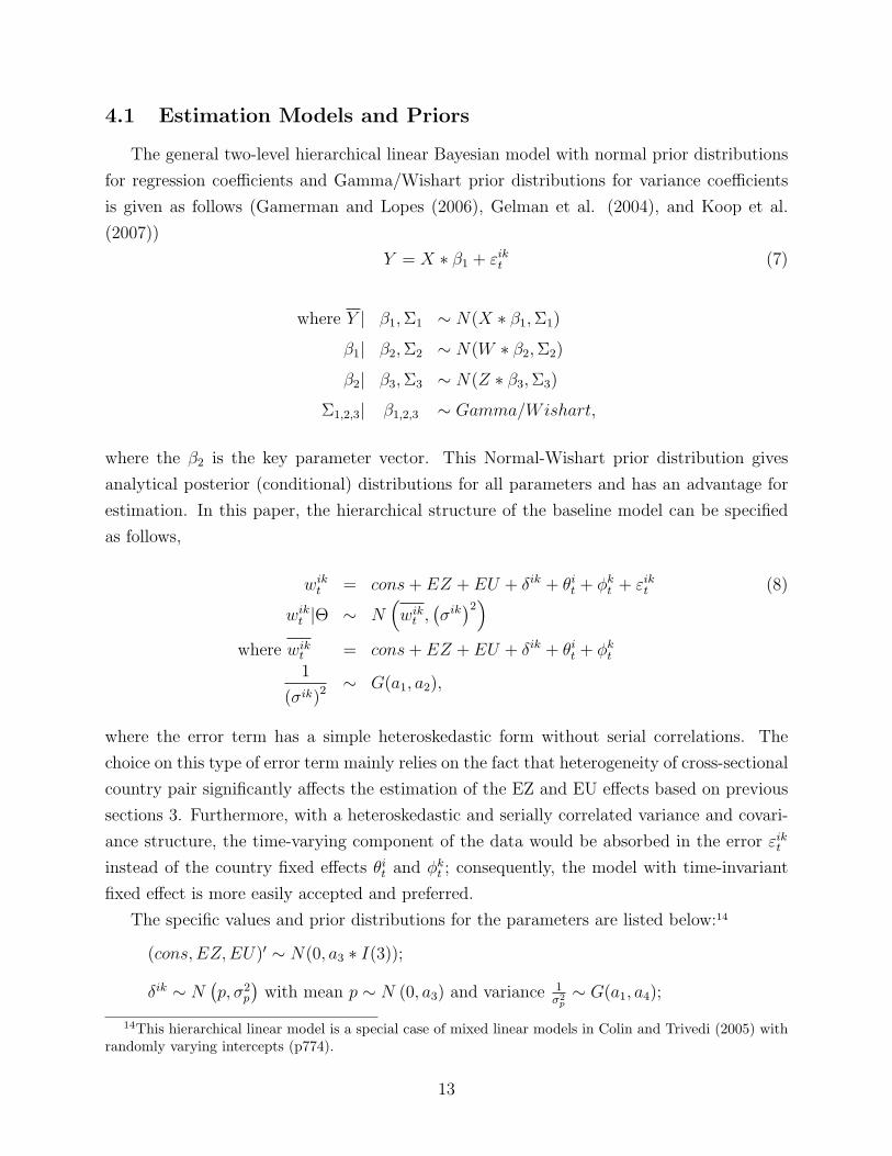
The general two-level hierarchical linear Bayesian model with normal prior distributions

for regression coefficients and Gamma/Wishart prior distributions for variance coefficients

is given as follows (Gamerman and Lopes (2006), Gelman et al. (2004), and Koop et al.

(2007))

Y = X ∗ β1 + εikt (7)

where Y | β1,Σ1 ∼ N(X ∗ β1,Σ1)

β1| β2,Σ2 ∼ N(W ∗ β2,Σ2)

β2| β3,Σ3 ∼ N(Z ∗ β3,Σ3)

Σ1,2,3| β1,2,3 ∼ Gamma/Wishart,

where the β2 is the key parameter vector. This Normal-Wishart prior distribution gives

analytical posterior (conditional) distributions for all parameters and has an advantage for

estimation. In this paper, the hierarchical structure of the baseline model can be specified

as follows,

wikt = cons+ EZ + EU + δik + θit + ϕk

t + εikt (8)

wikt |Θ ∼ N

(wik

t ,(σik)2)

where wikt = cons+ EZ + EU + δik + θit + ϕk

t

1

(σik)2∼ G(a1, a2),

where the error term has a simple heteroskedastic form without serial correlations. The

choice on this type of error term mainly relies on the fact that heterogeneity of cross-sectional

country pair significantly affects the estimation of the EZ and EU effects based on previous

sections 3. Furthermore, with a heteroskedastic and serially correlated variance and covari-

ance structure, the time-varying component of the data would be absorbed in the error εikt

instead of the country fixed effects θit and ϕkt ; consequently, the model with time-invariant

fixed effect is more easily accepted and preferred.

The specific values and prior distributions for the parameters are listed below:14

(cons, EZ,EU)′ ∼ N(0, a3 ∗ I(3));

δik ∼ N(p, σ2

p

)with mean p ∼ N (0, a3) and variance 1

σ2p∼ G(a1, a4);

14This hierarchical linear model is a special case of mixed linear models in Colin and Trivedi (2005) withrandomly varying intercepts (p774).

13

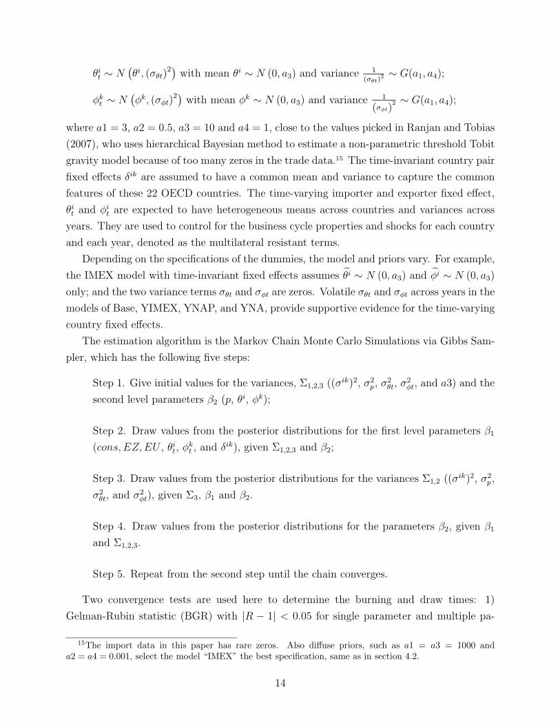
θit ∼ N(θi, (σθt)

2) with mean θi ∼ N (0, a3) and variance 1(σθt)

2 ∼ G(a1, a4);

ϕkt ∼ N

(ϕk, (σϕt)

2) with mean ϕk ∼ N (0, a3) and variance 1

(σϕt)2 ∼ G(a1, a4);

where a1 = 3, a2 = 0.5, a3 = 10 and a4 = 1, close to the values picked in Ranjan and Tobias

(2007), who uses hierarchical Bayesian method to estimate a non-parametric threshold Tobit

gravity model because of too many zeros in the trade data.15 The time-invariant country pair

fixed effects δik are assumed to have a common mean and variance to capture the common

features of these 22 OECD countries. The time-varying importer and exporter fixed effect,

θit and ϕit are expected to have heterogeneous means across countries and variances across

years. They are used to control for the business cycle properties and shocks for each country

and each year, denoted as the multilateral resistant terms.

Depending on the specifications of the dummies, the model and priors vary. For example,

the IMEX model with time-invariant fixed effects assumes θi ∼ N (0, a3) and ϕi ∼ N (0, a3)

only; and the two variance terms σθt and σϕt are zeros. Volatile σθt and σϕt across years in the

models of Base, YIMEX, YNAP, and YNA, provide supportive evidence for the time-varying

country fixed effects.

The estimation algorithm is the Markov Chain Monte Carlo Simulations via Gibbs Sam-

pler, which has the following five steps:

Step 1. Give initial values for the variances, Σ1,2,3 ((σik)2, σ2

p, σ2θt, σ

2ϕt, and a3) and the

second level parameters β2 (p, θi, ϕk);

Step 2. Draw values from the posterior distributions for the first level parameters β1

(cons, EZ,EU , θit, ϕkt , and δik), given Σ1,2,3 and β2;

Step 3. Draw values from the posterior distributions for the variances Σ1,2 ((σik)2, σ2p,

σ2θt, and σ2

ϕt), given Σ3, β1 and β2.

Step 4. Draw values from the posterior distributions for the parameters β2, given β1

and Σ1,2,3.

Step 5. Repeat from the second step until the chain converges.

Two convergence tests are used here to determine the burning and draw times: 1)

Gelman-Rubin statistic (BGR) with |R − 1| < 0.05 for single parameter and multiple pa-

15The import data in this paper has rare zeros. Also diffuse priors, such as a1 = a3 = 1000 anda2 = a4 = 0.001, select the model “IMEX” the best specification, same as in section 4.2.

14

rameters (Gelman (2006));16 2) Geweke chi-squared test (Geweke (1992)).17 Most of the

parameters in the small models like IMEXYear, IMEX, NAYear, and YearPair converge af-

ter 5000 burning times based on the two tests. However, the large models have more than one

thousand parameters and converge slowly. After 100,000 burning times, parameters in all

models have converged based on BGR statistics for 50000 draws (thin 10) from either single

chain or multiple chains. Coefficients in small models and the second level (key) parameters

(β2) in large models converged based on Geweke Chi-squared statistics.

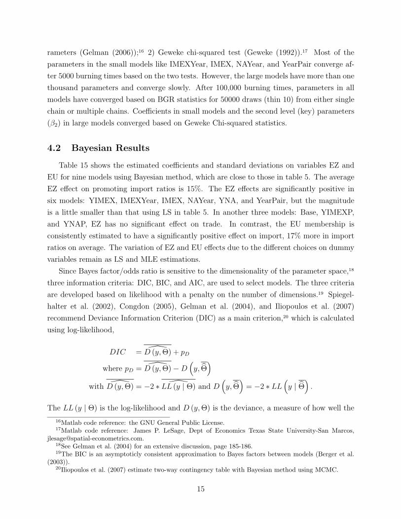
4.2 Bayesian Results

Table 15 shows the estimated coefficients and standard deviations on variables EZ and

EU for nine models using Bayesian method, which are close to those in table 5. The average

EZ effect on promoting import ratios is 15%. The EZ effects are significantly positive in

six models: YIMEX, IMEXYear, IMEX, NAYear, YNA, and YearPair, but the magnitude

is a little smaller than that using LS in table 5. In another three models: Base, YIMEXP,

and YNAP, EZ has no significant effect on trade. In comtrast, the EU membership is

consistently estimated to have a significantly positive effect on import, 17% more in import

ratios on average. The variation of EZ and EU effects due to the different choices on dummy

variables remain as LS and MLE estimations.

Since Bayes factor/odds ratio is sensitive to the dimensionality of the parameter space,18

three information criteria: DIC, BIC, and AIC, are used to select models. The three criteria

are developed based on likelihood with a penalty on the number of dimensions.19 Spiegel-

halter et al. (2002), Congdon (2005), Gelman et al. (2004), and Iliopoulos et al. (2007)

recommend Deviance Information Criterion (DIC) as a main criterion,20 which is calculated

using log-likelihood,

DIC = D (y,Θ) + pD

where pD = D (y,Θ)−D(y, Θ

)with D (y,Θ) = −2 ∗ LL (y | Θ) and D

(y, Θ

)= −2 ∗ LL

(y | Θ

).

The LL (y | Θ) is the log-likelihood and D (y,Θ) is the deviance, a measure of how well the

16Matlab code reference: the GNU General Public License.17Matlab code reference: James P. LeSage, Dept of Economics Texas State University-San Marcos,

jlesage@spatial-econometrics.com.18See Gelman et al. (2004) for an extensive discussion, page 185-186.19The BIC is an asymptoticly consistent approximation to Bayes factors between models (Berger et al.

(2003)).20Iliopoulos et al. (2007) estimate two-way contingency table with Bayesian method using MCMC.

15

model fits the data. The symbol “— ” refers to mean of the variables. The posterior mean

deviance D (y,Θ) is equal to -2 times the mean of posterior log-likelihood LL (y | Θ), and

the deviance D(y, Θ

)uses the log-likelihood calculated by the mean of posterior parameters

Θ. The pD, represents the penalty with a larger number of parameters. The smaller number

of DIC implies a better fit of the model. Another two commonly used criteria are Akaike

Information Criterion(AIC) and Bayesian Information Criterion (BIC) (Congdon (2005) and

Iliopoulos et al. (2007)) shown as below,

AIC = D(y, Θ

)+ 2 ∗ d

BIC = D(y, Θ

)+ d ∗ log (N)

where d is the (effective) number of estimated parameters and N is the number of obser-

vations. Smaller values in AIC and BIC indicate better fitness of the model. In table 15,

all three criteria give the lowest values for the model “IMEX” with time-invariant importer

and exporter fixed effects, and hence favor this specification to other eight models. If we cal-

culate the traditional LR statistics using the posterior log-likelihood LL(y | Θ

), the model

IMEX cannot be rejected by any other model who has a higher posterior log-likelihood (Base,

YIMEX, and YNA).

The supportive evidence for the model IMEX can also be found in figure 5 with fairly

constant posterior means for the variances of time-varying fixed effects. Figure 5 shows 95%

posterior credible intervals for the variances σ2θt and σ2

ϕt in three models with time-varying

fixed effects. The top two graphs are for the variances of time-varying importer and exporter

fixed effects σ2θt and σ2

ϕt respectively in the baseline model;21 and the bottom two are for the

variances of time-varying nation fixed effects in models YNA and YNAP. The non-volatile

variances give another evidence to favor the model IMEX with time-invariant dummies.

5 Conclusion

This paper studies how the choice of dummy variables affects the magnitude of the

Euro Zone effect on increasing bilateral import when we estimate gravity models. Three

groups of dummies, which are included in the gravity equations to control for individual

country and country-pair fixed effects, are compared, asymmetric or symmetric country pair

dummies, time-varying or time-invariant country dummies, separating importer/exporter or

nation dummies. Depending on the choice of dummies, EZ and EU effects on trade during

21The model YIMEX has similar posterior distributions of σ2θt and σ2

ϕt.

16

the period 1980–2004 vary greatly using the LS and MLE methods, from -0.3% to 49%.

Based on LS, conventional Wald test, LR test and F test are used to assess the necessity

of the different dummies; but these tests have a large size distortion/biased Chi-square

distributions. Two factors contribute this large size distortion. First the high dimensionality

of the parameter space leads to a biased asympotical chi-square distribution for LR test and

Wald tests. Second, hundreds of constraints associated with the hypothesis tests drive the

size distortion sensitive to the dimension adjustment method applied to the test statistics.

Among the issue on selecting three groups of dummies, it is the most difficult to make

a choice on time-varying or constant country dummies. Results from LS regressions and

Monte Carlo simulations on size distortions for the tests more or less show that symmetric

pair dummies influence the estimated coefficients similarly to the asymmetric pair effects,

and that separating the role of importer and exporter in the estimations does not signif-

icantly change the coefficients estimated from the model with symmetric nation dummies

only. However, there is no deterministic evidence against or for the time-varying country

dummies. Hence, hierarchical Bayesian method is adopted to provide the distributions of

all parameters and give a close investigation on the variances of the time-varying country

fixed effects. The non-volatile posterior distributions of the variance parameters in the mod-

els with time-varying country dummies provide evidence on the constant country effects.

Three information criteria based on Bayesian results also show that the model “IMEX” with

constant importer and exporter effects is favored among all nine models.

17

References

J.E. Anderson and E. Van Wincoop. Gravity with gravitas: a solution to the border puzzle. American

Economic Review, 93(1):170–192, 2003.

A. Aviat and N. Coeurdacier. The geography of trade in goods and asset holdings. Journal of International

Economics, 71(1):22–51, 2007.

R. Baldwin and D. Taglioni. Gravity for dummies and dummies for gravity equations. C.E.P.R. Discussion

Papers, Sep 2006.

J.O. Berger, J.K. Ghosh, and N. Mukhopadhyay. Approximations and consistency of Bayes factors as model

dimension grows. Journal of Statistical Planning and Inference, 112(1-2):241–258, 2003.

C.A. Colin and P.K. Trivedi. Microeconometrics: Methods and applications, 2005.

P. Congdon. Bayesian Models for Categorical Data. Chichester, United Kingdom John Wiley and Sons Ltd,

2005.

G.B.A Evans and N.E. Savin. Conflict among the criteria revisited: The w, lr and lm tests. Econometrica,

50(3):737–48, May 1982.

R.C. Feenstra and O.S. Drive. Border effects and the gravity equation: consistent methods for estimation.

Scottish Journal of Political Economy, 49:491–506, 2002.

A. Gelman. Prior distributions for variance parameters in hierarchical models. Bayesian Analysis, 1(3):

515–533, 2006.

A. Gelman, J. Carlin, H.S. Stern, and D.B. Rubin. Bayesian Data Analysis. New York, NY: Chapman and

Hall, 2004.

J. Geweke. Evaluating the accuracy of sampling-based approaches to the calculation of posterior moments.

Bayesian statistics, 4(2):169–193, 1992.

M. Guo. Frictions, heterogeneous preferences and international consumption risk sharing. University of

California, Davis. Manuscript, August 2010.

K. Head and T. Mayer. The Empirics of Agglomeration and Trade, in Handbook of Regional and Urban

Economics Vol.. Henderson, V. and JF Thisse, 2004.

G. Iliopoulos, M. Kateri, and I. Ntzoufras. Bayesian estimation of unrestricted and order-restricted as-

sociation models for a two-way contingency table. Computational Statistics and Data Analysis, 51(9):

4643–4655, 2007.

A. Italianer. A small-sample correction for the likelihood ratio test. Economics Letters, 19(4):315–317, 1985.

D.S. Jacks, C.M. Meissner, and D. Novy. Trade Costs, 1870-2000. American Economic Review, 98(2):

529–534, 2008.

18

A. Micco, E. Stein, G. Ordonez, K.H. Midelfart, and J.M. Viaene. The currency union effect on trade: early

evidence from EMU. Economic Policy, 18(37):317–356, 2003.

W.K. Newey and K.D. West. A simple, positive semi-definite, heteroskedasticity and autocorrelation con-

sistent covariance matrix. Econometrica, 55(3):703–08, May 1987.

W.K. Newey and K.D. West. Automatic lag selection in covariance matrix estimation. Review of Economic

Studies, 61(4):631–53, October 1994.

P. Ranjan and L.J. Tobias. Bayesian inference for the gravity model. Journal of Applied Econometrics, 22

(4):817–838, 2007.

A.K. Rose. Do we really know that the wto increases trade? American Economic Review, 94(1):98–114,

2004.

A.K. Rose and T.D. Stanley. A meta-analysis of the effect of common currencies on international trade.

Meta-regression analysis: issues of publication bias in economics, page 53, 2005.

A.K. Rose and E. Van Wincoop. National money as a barrier to international trade: The real case for

currency union. American Economic Review, 91(2):386–390, 2001.

D.J. Spiegelhalter, N.G. Best, B.P. Carlin, and A. van der Linde. Bayesian measures of model complexity

and fit. Journal of the Royal Statistical Society. Series B, Statistical Methodology, pages 583–639, 2002.

A. Subramanian and S.J. Wei. The wto promotes trade, strongly but unevenly. Journal of International

Economics, 72(1):151–175, 2007.

19

A Gravity Models and Data

Two main choices on dependent variables have been considered by researchers in esti-

mating the gravity equation, trade levels and ratios. The level dependent variable can be

the log of bilateral (unidirectional) imports/exports, or the average/sum of imports and ex-

ports between countries, whereas the later one suffers from the silver medal error proposed

by Baldwin and Taglioni (2006). These trade flow data can be measured by current dollar

or deflated by price index (US CPI). However, estimations with deflated trade values suffer

from the bronze medal error shown in Baldwin and Taglioni (2006). The model with log of

bilateral import levels is shown as below,

limikt = cons+ lyy + EZ + EU + δik + θit + ϕk

t +J∑

j=1

γjtgikjt + εikt . (9)

The dependent variable, limikt , is the log of bilateral import levels, log(IM ik

t ), which is

determined by heterogeneous preferences (δik ≡ log(αik)) , the product of importers’ ex-

penditures and exporters’ outputs (lyy ≡ log(EXP it ∗OUT k

t )), trade costs (gikjt ≡ log(τ ikt ))

and fixed effects. The trade costs gikjt include log of distance, dummies for border, common

language, land-lock, Euro Zone and European Union. With symmetric conditions, τ ikt = τ kit

and αi (k) = αk (i), trade balance for each country is zero and total output is equal to total

expenditure, EXP it = OUT i

t , so that lyy = log(OUT it ∗ OUT k

t ) if replacing expenditure

EXP it using output OUT i

t .

This type of estimation has a potential endogeniety problem because the economic mass

data “lyy” are included in the explanatory variables. Therefore, researchers use the second

choice: the log of the bilateral import ratio— imports divided by the product of the im-

porter’s expenditure and exporter’s output as in Anderson and Van Wincoop (2003) with

cross-section data. This estimation restricts the unit effect of economic mass variables on bi-

lateral trade. The model using bilateral import ratios in Anderson and Van Wincoop (2003)

and Aviat and Coeurdacier (2007) is given below,

limrikt = cons++EZ + EU + δik + θit + ϕkt +

J∑j=1

γjtgikjt + εikt , (10)

where the dependent variable is defined as

limrikt = log(IM ik

t

OUT it ∗OUT k

t

) or log(IM ik

t

EXP it ∗OUT k

t

).

The version of bilateral import ratios may be non-stationary with long panel data. Hence,

20

as in section 3 of Guo (2010), this paper uses the import ratios in equation (2) of section 2.1

limrikt = log(IM ik

t ∗WOUTt

OUT it ∗OUT k

t

).

The data contain 22 OECD countries. There are fourteen countries in EU by 1995—

AUT, BEL-LUX, DEU, DNK, ESP, FIN, FRA, GBR, GRC, IRL, ITA, NLD, PRT, and

SWE, among which four countries did not join in the EZ in 2000—DNK, GBR, GRC, and

SWE. Another eight countries—AUS, CAN, CHE, JPN, USA, ISL, NOR, and NZL— do

not belong to EU. The data source is listed as below,

1) Current dollar value of bilateral import/export data: IMF DOTS.

2) Current dollar value of GDP: WDI and IMF DOTS (robustness check).

3) Current dollar value of private consumption expenditure: World Bank’s World De-

velopment Indicators (WDI).

4) Bilateral trade costs variables: distance, dummies for border connection, landlock,

and common language are taken from CEPII. Geodesic (great circle) distances are

measured as kilometers between capital cities.22

5) EU and EZ dummies: constructed by author following the dates of countries’ par-

ticipation in European Union and Euro Zone.

B Monte Carlo Simulations

B.1 Size under Homoscedastic Errors

All models with different groups of dummy variables are nested in the baseline model. I

use the baseline model (the alternative) and the model “IMEX” (the null) as an example to

illustrate the Monte Carlo simulations for size distortion presented in table 10

wikt = cons+ EZ + EU + δik + (θit + θi) + (ϕk

t + ϕk) +3∑

j=1

γjtgikj + εikt ,

where θit = θit + θi and ϕkt = ϕk

t + ϕk. In order to obtain the model “IMEX”, we need to

impose the following 1448 restrictions on the baseline model: δik = 0, θit = 0, and ϕkt = 0.

All simulations are performed 1000 times.

22http://www.cepii.franglaisgraph /bdd/distances.htm

21

1) Obtain the coefficients B0 (θi, ϕk, EU, EZ, γjt and the constant intercept) and

variance σ20 (=var(ϵ0)) based on the model y = XB0 + ϵ0. I estimate the coefficients

from the model “IMEX” using the real data shown in appendix A. The dependent

variable is import ratio log(

(1+IM ikt )∗WOUTt

EXP it ∗OUTk

t

). The coefficients on trade costs γjt are

listed in table 5. The variance is the mean of the squared residual.

2) Simulate the dependent variables y for 1000 times given B0, σ20, and the covariates

X from the model “IMEX”. The random sample comes from the random draws of the

error term.

3) Fit the simulated y using both the null and alternative models ( y = XBm + ϵj

and m ∈ n, a, the subscript“n” and “a” is represented the the null and alternative

models respectively. ) and obtain the estimated coefficients (Bn and Ba) and variance

(σ2n and σ2

a) for 1000 times assuming i.i.d.

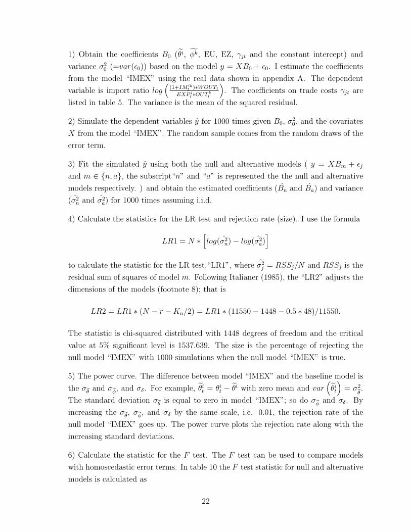
4) Calculate the statistics for the LR test and rejection rate (size). I use the formula

LR1 = N ∗[log(σ2

n)− log(σ2a)]

to calculate the statistic for the LR test,“LR1”, where σ2j = RSSj/N and RSSj is the

residual sum of squares of model m. Following Italianer (1985), the “LR2” adjusts the

dimensions of the models (footnote 8); that is

LR2 = LR1 ∗ (N − r −Kn/2) = LR1 ∗ (11550− 1448− 0.5 ∗ 48)/11550.

The statistic is chi-squared distributed with 1448 degrees of freedom and the critical

value at 5% significant level is 1537.639. The size is the percentage of rejecting the

null model “IMEX” with 1000 simulations when the null model “IMEX” is true.

5) The power curve. The difference between model “IMEX” and the baseline model is

the σθ and σϕ, and σδ. For example, θit = θit − θi with zero mean and var(θit

)= σ2

θ.

The standard deviation σθ is equal to zero in model “IMEX”; so do σϕ and σδ. By

increasing the σθ, σϕ, and σδ by the same scale, i.e. 0.01, the rejection rate of the

null model “IMEX” goes up. The power curve plots the rejection rate along with the

increasing standard deviations.

6) Calculate the statistic for the F test. The F test can be used to compare models

with homoscedastic error terms. In table 10 the F test statistic for null and alternative

models is calculated as

22

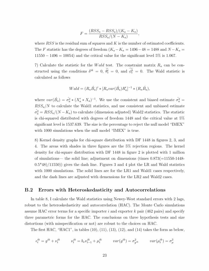
F =(RSSn −RSSa)/(Ka −Kn)

RSSa/(N −Ka),

where RSS is the residual sum of squares andK is the number of estimated coefficients.

The F statistic has the degrees of freedom (Ka−Kn = 1496−48 = 1488 and N−Ka =

11550− 1496 = 10054) and the critical value for the significant level 5% is 1.067.

7) Calculate the statistic for the Wald test. The constraint matrix Rn can be con-

structed using the conditions δik = 0, θit = 0, and ϕkt = 0. The Wald statistic is

calculated as follows

Wald = (RnBa)′ ∗ [Rnvar(Ba)R

′n]

−1 ∗ (RnBa),

where var(Ba) = σ2a ∗ (X ′

a ∗ Xa)−1. We use the consistent and biased estimate σ2

a =

RSSa/N to calculate the Wald1 statistics, and use consistent and unbiased estimate

σ2a = RSSa/(N −Ka) to calculate (dimension adjusted) Wald2 statistics. The statistic

is chi-squared distributed with degrees of freedom 1448 and the critical value at 5%

significant level is 1537.639. The size is the percentage to reject the null model “IMEX”

with 1000 simulations when the null model “IMEX” is true.

8) Kernel density graphs for chi-square distribution with DF 1448 in figures 2, 3, and

4. The areas with shades in three figures are the 5% rejection regions. The kernel

density for chi-square distribution with DF 1448 in figure 2 is plotted with 1 million

of simulations— the solid line; adjustment on dimensions (times 0.873(=11550-1448-

0.5*48)/11550)) gives the dash line. Figures 3 and 4 plot the LR and Wald statistics

with 1000 simulations. The solid lines are for the LR1 and Wald1 cases respectively,

and the dash lines are adjusted with demensions for the LR2 and Wald2 cases.

B.2 Errors with Heteroskedasticity and Autocorrelations

In table 8, I calculate the Wald statistics using Newey-West standard errors with 2 lags,

robust to the heteroskedasticity and autocorrelation (HAC). The Monte Carlo simulations

assume HAC error terms for a specific importer i and exporter k pair (462 pairs) and specify

three parametric forms for the HAC. The conclusions on three hypothesis tests and size

distortions (with misspecification or not) are robust to the choices on HAC.

The first HAC, “HAC1”, in tables (10), (11), (13), (12), and (14) takes the form as below,

ϵikt = gik + νikt νik

t = bννikt−1 + µik

t var(gik) = σ2gik var(µik

t ) = σ2µ

23

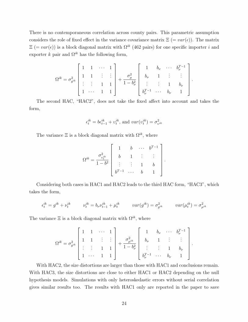
There is no contemporaneous correlation across county pairs. This parametric assumption

considers the role of fixed effect in the variance covariance matrix Ξ (= var(ϵ)). The matrix

Ξ (= var(ϵ)) is a block diagonal matrix with Ωik (462 pairs) for one specific importer i and

exporter k pair and Ωik has the following form,

Ωik = σ2gik

1 1 · · · 1

1 1...

......

... 1 1

1 · · · 1 1

+σ2µ

1− b2ν

1 bν · · · bT−1

ν

bν 1...

......

... 1 bν

bT−1ν · · · bν 1

.

The second HAC, “HAC2”, does not take the fixed affect into account and takes the

form,

ϵikt = bϵikt−1 + υikt , and var(υik

t ) = σ2υik

The variance Ξ is a block diagonal matrix with Ωik, where

Ωik =σ2υikt

1− b2

1 b · · · bT−1

b 1...

......

... 1 b

bT−1 · · · b 1

.

Considering both cases in HAC1 and HAC2 leads to the third HAC form, “HAC3”, which

takes the form,

ϵikt = gik + νikt νik

t = bννikt−1 + µik

t var(gik) = σ2gik var(µik

t ) = σ2µik

The variance Ξ is a block diagonal matrix with Ωik, where

Ωik = σ2gik

1 1 · · · 1

1 1...

......

... 1 1

1 · · · 1 1

+σ2µik

1− b2ν

1 bν · · · bT−1

ν

bν 1...

......

... 1 bν

bT−1ν · · · bν 1

.

With HAC2, the size distortions are larger than those with HAC1 and conclusions remain.

With HAC3, the size distortions are close to either HAC1 or HAC2 depending on the null

hypothesis models. Simulations with only heteroskedastic errors without serial correlation

gives similar results too. The results with HAC1 only are reported in the paper to save

24

space.

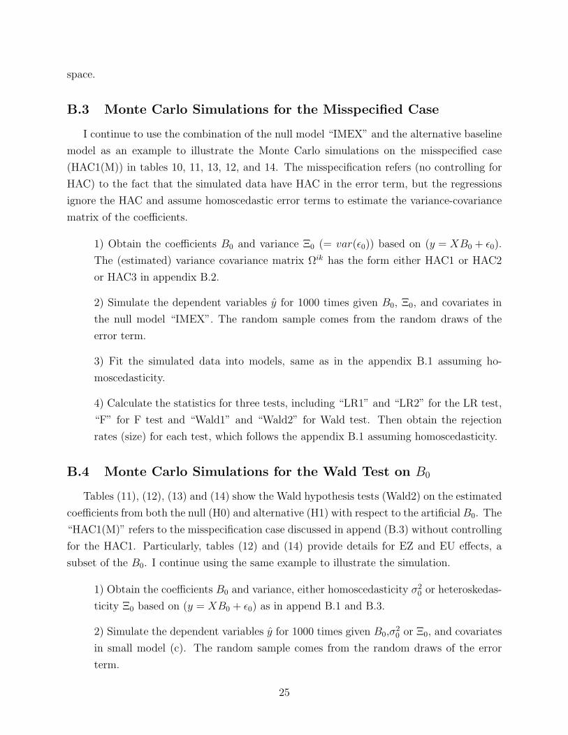
B.3 Monte Carlo Simulations for the Misspecified Case

I continue to use the combination of the null model “IMEX” and the alternative baseline

model as an example to illustrate the Monte Carlo simulations on the misspecified case

(HAC1(M)) in tables 10, 11, 13, 12, and 14. The misspecification refers (no controlling for

HAC) to the fact that the simulated data have HAC in the error term, but the regressions

ignore the HAC and assume homoscedastic error terms to estimate the variance-covariance

matrix of the coefficients.

1) Obtain the coefficients B0 and variance Ξ0 (= var(ϵ0)) based on (y = XB0 + ϵ0).

The (estimated) variance covariance matrix Ωik has the form either HAC1 or HAC2

or HAC3 in appendix B.2.

2) Simulate the dependent variables y for 1000 times given B0, Ξ0, and covariates in

the null model “IMEX”. The random sample comes from the random draws of the

error term.

3) Fit the simulated data into models, same as in the appendix B.1 assuming ho-

moscedasticity.

4) Calculate the statistics for three tests, including “LR1” and “LR2” for the LR test,

“F” for F test and “Wald1” and “Wald2” for Wald test. Then obtain the rejection

rates (size) for each test, which follows the appendix B.1 assuming homoscedasticity.

B.4 Monte Carlo Simulations for the Wald Test on B0

Tables (11), (12), (13) and (14) show the Wald hypothesis tests (Wald2) on the estimated

coefficients from both the null (H0) and alternative (H1) with respect to the artificial B0. The

“HAC1(M)” refers to the misspecification case discussed in append (B.3) without controlling

for the HAC1. Particularly, tables (12) and (14) provide details for EZ and EU effects, a

subset of the B0. I continue using the same example to illustrate the simulation.

1) Obtain the coefficients B0 and variance, either homoscedasticity σ20 or heteroskedas-

ticity Ξ0 based on (y = XB0 + ϵ0) as in append B.1 and B.3.

2) Simulate the dependent variables y for 1000 times given B0,σ20 or Ξ0, and covariates

in small model (c). The random sample comes from the random draws of the error

term.

25

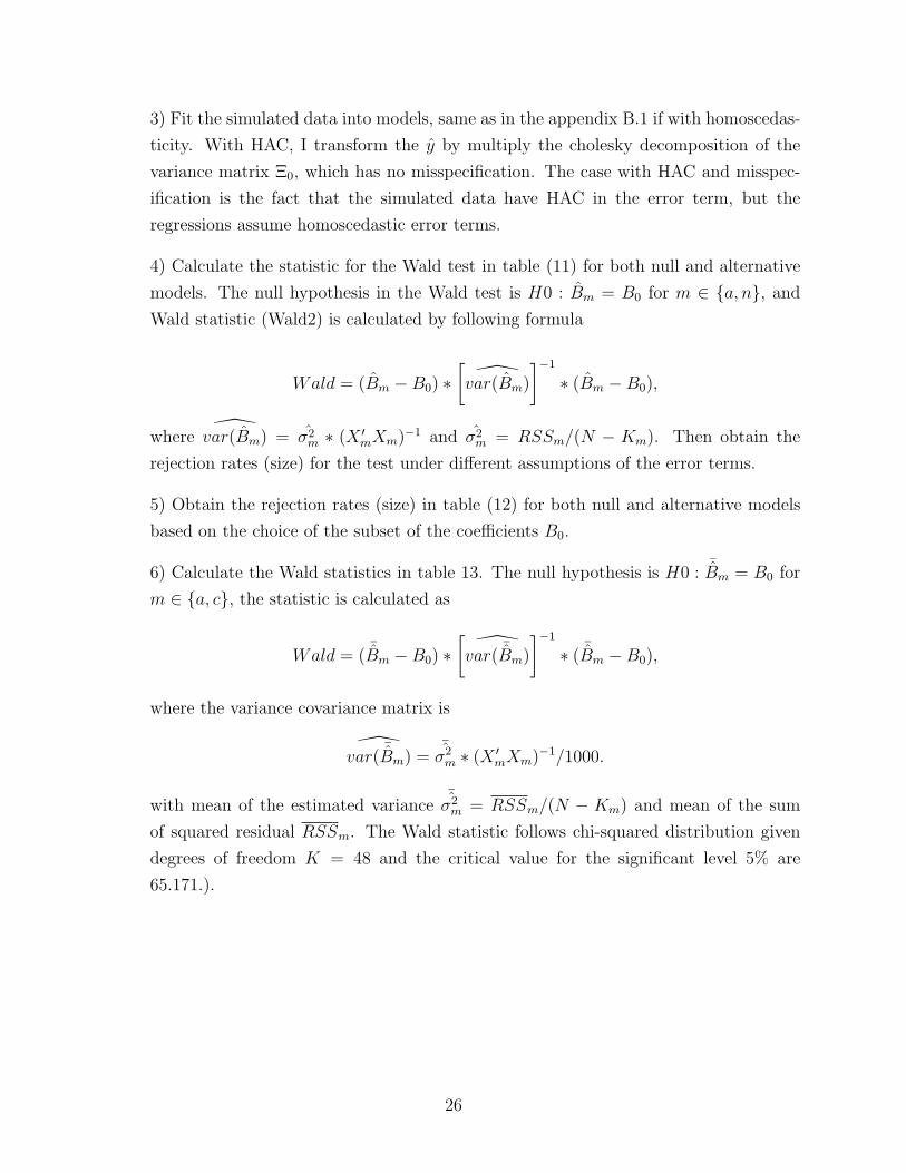
3) Fit the simulated data into models, same as in the appendix B.1 if with homoscedas-

ticity. With HAC, I transform the y by multiply the cholesky decomposition of the

variance matrix Ξ0, which has no misspecification. The case with HAC and misspec-

ification is the fact that the simulated data have HAC in the error term, but the

regressions assume homoscedastic error terms.

4) Calculate the statistic for the Wald test in table (11) for both null and alternative

models. The null hypothesis in the Wald test is H0 : Bm = B0 for m ∈ a, n, andWald statistic (Wald2) is calculated by following formula

Wald = (Bm −B0) ∗[

var(Bm)

]−1

∗ (Bm −B0),

where var(Bm) = σ2m ∗ (X ′

mXm)−1 and σ2

m = RSSm/(N − Km). Then obtain the

rejection rates (size) for the test under different assumptions of the error terms.

5) Obtain the rejection rates (size) in table (12) for both null and alternative models

based on the choice of the subset of the coefficients B0.

6) Calculate the Wald statistics in table 13. The null hypothesis is H0 :¯Bm = B0 for

m ∈ a, c, the statistic is calculated as

Wald = (¯Bm −B0) ∗

[

var(¯Bm)

]−1

∗ ( ¯Bm −B0),

where the variance covariance matrix is

var(

¯Bm) =

¯σ2m ∗ (X ′

mXm)−1/1000.

with mean of the estimated variance¯σ2m = RSSm/(N − Km) and mean of the sum

of squared residual RSSm. The Wald statistic follows chi-squared distribution given

degrees of freedom K = 48 and the critical value for the significant level 5% are

65.171.).

26

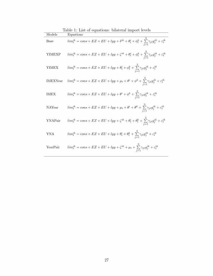
Table 1: List of equations: bilateral import levelsModels Equations

Base limikt = cons+ EZ + EU + lyy + δik + θit + ϕk

t +3∑

j=1

γjtgikj + εikt

YIMEXP limikt = cons+ EZ + EU + lyy + ζik + θit + ϕk

t +3∑

j=1

γjtgikj + εikt

YIMEX limikt = cons+ EZ + EU + lyy + θit + ϕk

t +3∑

j=1

γjtgikj + εikt

IMEXYear limikt = cons+ EZ + EU + lyy + µt + θi + ϕk +

3∑j=1

γjtgikj + εikt

IMEX limikt = cons+ EZ + EU + lyy + θi + ϕk +

3∑j=1

γjtgikj + εikt

NAYear limikt = cons+ EZ + EU + lyy + µt + θi + θk +

3∑j=1

γjtgikj + εikt

YNAPair limikt = cons+ EZ + EU + lyy + ζik + θit + θkt +

3∑j=1

γjtgikj + εikt

YNA limikt = cons+ EZ + EU + lyy + θit + θkt +

3∑j=1

γjtgikj + εikt

YearPair limikt = cons+ EZ + EU + lyy + ζik + µt +

3∑j=1

γjtgikj + εikt

27

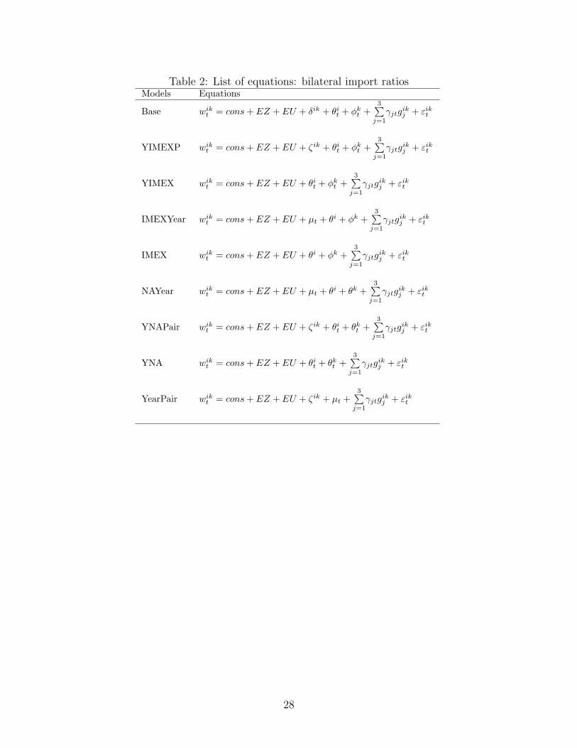
Table 2: List of equations: bilateral import ratiosModels Equations

Base wikt = cons+ EZ + EU + δik + θit + ϕk

t +3∑

j=1

γjtgikj + εikt

YIMEXP wikt = cons+ EZ + EU + ζik + θit + ϕk

t +3∑

j=1

γjtgikj + εikt

YIMEX wikt = cons+ EZ + EU + θit + ϕk

t +3∑

j=1

γjtgikj + εikt

IMEXYear wikt = cons+ EZ + EU + µt + θi + ϕk +

3∑j=1

γjtgikj + εikt

IMEX wikt = cons+ EZ + EU + θi + ϕk +

3∑j=1

γjtgikj + εikt

NAYear wikt = cons+ EZ + EU + µt + θi + θk +

3∑j=1

γjtgikj + εikt

YNAPair wikt = cons+ EZ + EU + ζik + θit + θkt +

3∑j=1

γjtgikj + εikt

YNA wikt = cons+ EZ + EU + θit + θkt +

3∑j=1

γjtgikj + εikt

YearPair wikt = cons+ EZ + EU + ζik + µt +

3∑j=1

γjtgikj + εikt

28

Tab

le3:

Euro

effectan

dEuropeanUnioneff

ecton

(log)bilateral

importlevelbyLS:1992-2002

Dummies

Base

1)YIM

EXP

2)YIM

EX

3)IM

EXYear4)

IMEX

5)NAYear6)

YNAP

7)YNA

8)YearP

air9)

OLS

Tim

e-varyingYes

Yes

Yes

No

No

No

Yes

Yes

No

No

Imp.&

Exp.Yes

Yes

Yes

Yes

Yes

No

No

No

No

No

Nation

No

No

No

No

No

Yes

Yes

Yes

No

No

Year

No

No

No

Yes

No

Yes

No

No

Yes

No

Pair

Asym.

Sym.

No

No

No

No

Sym.

No

Sym.

No

/Var.

EZ

-0.008

-0.008

0.34

9**

0.26

6**

0.26

7**

0.26

6**

-0.008

0.34

9**

0.12

0**

0.233**

0.03

90.03

80.10

70.05

20.04

40.05

20.03

70.10

50.02

80.048

EU

0.06

70.06

70.28

4*0.20

5

0.21

6*0.205

0.06

70.28

4*-0.006

0.052

0.04

70.04

60.14

40.10

50.10

10.10

50.04

50.14

00.03

20.088

lyy

1.17

2**0.92

3**

0.84

10.55

8**

0.60

9**

0.55

8**

0.85

0**

0.78

6**

0.52

3**

0.803**

0.01

30.02

20.03

60.05

70.04

30.05

70.00

90.04

30.05

50.020

locked

im-1.493

**-0.328**

0.06

30.101

locked

ex-1.661

**-0.496**

0.06

40.115

log(dist.)

-0.880

**-0.897

**-0.895

**-0.897

**-0.880

**-0.763**

0.07

50.06

90.06

90.06

90.07

30.044

contig.

0.22

30.21

70.21

80.21

70.22

30.329*

0.14

20.13

60.13

60.13

50.13

80.128

comlang.

0.39

1**

0.38

4**

0.38

5**

0.38

4**

0.39

1**

0.624**

0.11

20.10

80.10

80.10

80.11

00.126

Obs.

5082

5082

5082

5082

5082

5082

5082

5082

5082

5082

RSS

150.3

550

1450

1512

1517

1932

995

1895

1019

2646

Adj.R2

0.99

30.97

50.93

50.93

20.93

20.91

30.95

50.91

50.95

40.881

LL

1735

-156

1-402

4-413

1-414

0-475

4-306

7-470

4-312

8-5553

This

table

replicatestable

4in

Baldwin

andTag

lion

i(200

6).**

sign

ificantat

1%;*sign

ificantat

5%;sign

ificantat

10%.Thestan

darderrors

reportedbelow

thecoeffi

cientestimates

forallmodelsareclustered

ontime-invarian

tcountry

pairs.“L

L”isthelog-likelihoodbased

oni.i.d.errors.“E

Z”variab

leisthedummyforEuro

Zon

e,takingon

ewhen

both

countriesarein

theeu

rozonean

dzero

when

atleaston

ecountryisnot

intheeu

rozone.

“EU”variab

leisthedummyfor

EuropeanUnion,takingon

eifcountrypairs

aremem

bersof

EuropeanUnion(tracingbackto

EuropeanCoa

lan

dSteel

Com

munityan

dTreatyof

Rom

e).

29

Tab

le4:

Euro

effectan

dEuropeanUnioneff

ecton

(log)bilateral

importlevelbyLS:1980-2004

Dummies

Base

1)YIM

EXP

2)YIM

EX

3)IM

EXYear4)

IMEX

5)NAYear6)

YNAP

7)YNA

8)YearP

air9)

OLS

Tim

e-varyingYes

Yes

Yes

No

No

No

Yes

Yes

No

No

Imp.&

Exp.Yes

Yes

Yes

Yes

Yes

No

No

No

No

No

Nation

No

No

No

No

No

Yes

Yes

Yes

No

No

Year

No

No

No

Yes

No

Yes

No

No

Yes

No

Pair

Asym.

Sym.

No

No

No

No

Sym.

No

Sym.

No

/Var.

EZ

-0.004

-0.004

0.41

3**

0.33

0**

0.31

4**

0.33

0**

-0.004

0.41

3**

0.16

6**

0.009

0.05

50.05

50.11

20.05

70.05

10.05

70.05

30.11

00.03

70.054

EU

0.22

7**0.22

7**

0.17

10.15

6*0.16

7*0.15

6*0.22

7**

0.17

10.17

5**

0.008

0.05

60.05

50.11

20.07

40.07

20.07

40.05

40.10

90.03

90.078

lyy

1.06

2**0.86

7**

0.76

6**

0.58

4**

0.50

8**

0.58

4**

0.90

4**

0.77

3**

0.60

2**

0.767**

0.02

10.02

70.03

70.05

80.01

30.05

70.01

50.04

50.05

70.019

locked

im-1.350

**-0.320**

0.05

50.095

locked

ex-1.522

**-0.492**

0.05

80.107

log(dist.)

-0.890

**-0.894

**-0.893

**-0.894

**-0.890

**-0.765**

0.06

90.06

40.06

40.06

40.06

70.041

contig.

0.21

20.21

2

0.21

20.212

0.21

20.410**

0.13

00.12

50.12

50.12

50.12

70.122

comlang.

0.42

4**

0.42

2**

0.42

3**

0.42

2**

0.42

4**

0.614**

0.10

90.10

50.10

50.10

50.10

70.124

Obs.

1155

011

550

1155

011

550

1155

011

550

1155

011

550

1155

011550

RSS

751.6

1615

3463

3775

3801

4505

2504

4351

2646

6782

Adj.R2

0.98

40.96

60.92

80.92

80.92

80.91

50.94

90.91

40.94

90.872

LL

-610

-502

9-943

3-993

1-997

0-109

51-755

9-107

51-787

9-13314

This

table

replicatesthetable

5in

Baldwin

andTag

lion

i(200

6).See

table

notes

intable

3.

30

Tab

le5:

Euro

effectan

dEuropeanUnioneff

ecton

(log)bilateral

importratiobyLS:1980-2004

Dummies

Base

1)YIM

EXP

2)YIM

EX

3)IM

EXYear4)

IMEX

5)NAYear6)

YNAP

7)YNA

8)YearP

air9)

OLS

Tim

e-varyingYes

Yes

Yes

No

No

No

Yes

Yes

No

No

Imp.&

Exp.Yes

Yes

Yes

Yes

Yes

No

No

No

No

No

Nation

No

No

No

No

No

Yes

Yes

Yes

No

No

Year

No

No

No

Yes

No

Yes

No

No

Yes

No

Pair

Asym.

Sym.

No

No

No

No

Sym.

No

Sym.

No

/Var.

EZ

-0.003

-0.003

0.24

0**

0.20

3**

0.40

2**

0.20

3**

-0.003

0.24

0**

0.10

9**

0.277**

0.03

30.03

20.06

80.03

50.03

20.03

50.03

10.06

60.02

30.053

EU

0.13

5**0.13

5**

0.08

80.08

30.28

7**

0.08

3

0.13

5**

0.08

80.10

3**

0.313**

0.03

30.03

30.06

90.04

60.04

50.04

60.03

20.06

70.02

40.084

locked

im-2.087

**-0.187*

0.04

10.090

locked

ex-2.188

**-0.289**

0.03

80.100

log(dist.)

-0.518

**-0.520

**-0.483

**-0.520

**-0.518

**-0.324**

0.04

30.04

00.04

20.04

00.04

20.043

contig.

0.09

90.09

90.09

60.09

90.09

90.487**

0.07

90.07

60.07

70.07

60.07

80.110

comlang.

0.25

9**

0.25

8**

0.28

4**

0.25

8**

0.25

9**

0.495**

0.06

60.06

30.06

40.06

30.06

40.109

Obs.

1155

011

550

1155

011

550

1155

011

550

1155

011

550

1155

011550

RSS

274.4

588.2

1269

1380

1939

1633

896

1577

949.7

5746.6

Adj.R2

0.96

80.93

20.85

70.85

80.80

10.83

20.90

20.83

00.90

10.411

LL

5208

805.6

-363

6-412

0-608

4-509

3-162

5-489

0-196

1-12357

See

table

notes

intable

3.

31

Tab

le6:

Euro

effectan

dEuropeanUnioneff

ecton

(log)bilateral

importlevelbyMLE:1980-2004

Dummies

Base

1)YIM

EXP

2)YIM

EX

3)IM

EXYear4)

IMEX

5)NAYear6)

YNAP

7)YNA

8)YearP

air9)

OLS

Tim

e-varyingYes

Yes

Yes

No

No

No

Yes

Yes

No

No

Imp.&

Exp.Yes

Yes

Yes

Yes

Yes

No

No

No

No

No

Nation

No

No

No

No

No

Yes

Yes

Yes

No

No

Year

No

No

No

Yes

No

Yes

No

No

Yes

No

Pair

Asym.

Sym.

No

No

No

No

Sym.

No

Sym.

No

/Var.

EZ

-0.004

-0.004

0.00

20.16

9**

0.17

7**

0.16

8**

-0.004

0.00

10.16

6**

0.16

8**

0.02

20.02

30.02

30.01

70.01

50.01

70.02

50.02

50.01

70.01

5EU

0.22

7**0.22

7**

0.22

6**

0.17

5**

0.18

8**

0.17

5**

0.22

7**

0.22

7**

0.17

5**

0.17

9**

0.01

80.01

80.01

80.01

40.01

40.01

40.02

00.02

00.01

40.01

4lyy

1.12

0**0.91

4**

0.80

6**

0.60

2**

0.51

4**

0.60

2**

0.90

4**

0.78

3**

0.60

2**

0.52

3**

0.00

20.00

40.00

90.01

80.00

40.01

80.10

80.04

40.01

80.00

4locked

im-1.350

**-0.379

0.37

20.14

5locked

ex-1.522

**-0.552

0.37

20.14

5log(dist.)

-0.890

**-0.895

**-0.892

**-0.895

**-0.890

**-0.668

**0.04

70.04

70.04

60.05

20.05

30.04

0contig.

0.21

00.21

1

0.21

10.21

1

0.21

00.71

8**

0.10

90.10

80.10

80.12

20.12

30.17

9comlang.

0.43

0**

0.42

4**

0.42

6**

0.42

4**

0.43

0**

0.73

4**

0.09

20.09

20.09

20.10

40.10

40.13

7sigm

au

0.00

00.26

80.48

40.48

10.48

10.54

30.36

70.54

50.36

40.88

10.00

20.00

90.01

60.01

60.01

60.01

80.01

20.01

80.01

20.03

0sigm

ae

0.25

50.26

00.26

00.31

00.31

40.31

00.28

60.28

60.31

00.31

40.00

20.00

20.00

20.00

20.00

20.00

20.00

20.00

20.00

20.00

2rho

0.00

00.51

50.77

60.70

60.70

10.75

40.62

10.78

40.58

00.88

7Obs.

1155

011

550

1155

011

550

1155

011

550

1155

011

550

1155

011

550

R2-P

0.97

60.86

40.84

10.67

70.66

60.67

30.76

20.74

70.68

80.64

3LL

-610

-161

2-187

9-382

1-395

3-387

6-281

4-299

3-369

6-423

3

**sign

ificantat

1%;*sign

ificantat

5%;sign

ificantat

10%.MLE

assumes

therandom

effects,i.e.

ϵik t=

uik

+ei

k t,

var(uik)=

σ2 uan

dvar(ei

k t)=

σ2 e.

32

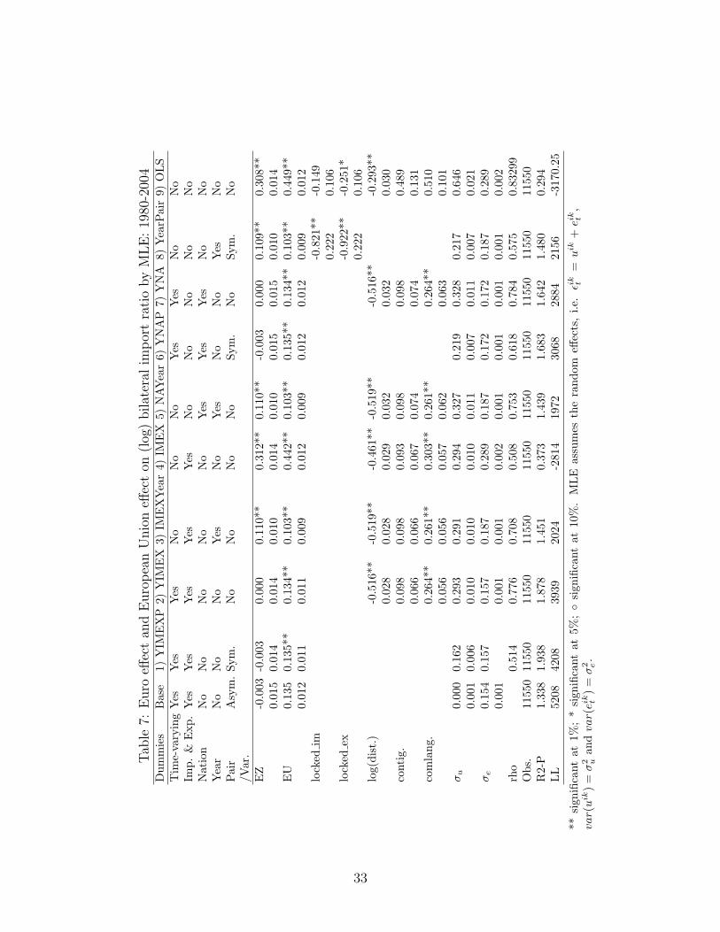
Tab

le7:

Euro

effectan

dEuropeanUnioneff

ecton

(log)bilateral

importratiobyMLE:1980-2004

Dummies

Base

1)YIM

EXP

2)YIM

EX

3)IM

EXYear4)

IMEX

5)NAYear6)

YNAP

7)YNA

8)YearP

air9)

OLS

Tim

e-varyingYes

Yes

Yes

No

No

No

Yes

Yes

No

No

Imp.&

Exp.Yes

Yes

Yes

Yes

Yes

No

No

No

No

No

Nation

No

No

No

No

No

Yes

Yes

Yes

No

No

Year

No

No

No

Yes

No

Yes

No

No

Yes

No

Pair

Asym.Sym.

No

No

No

No

Sym.

No

Sym.

No

/Var.

EZ

-0.003

-0.003

0.00

00.11

0**

0.31

2**

0.11

0**

-0.003

0.00

00.10

9**

0.308**

0.01

50.01

40.01

40.01

00.01

40.01

00.01

50.01

50.01

00.014

EU

0.13

50.13

5**

0.13

4**

0.10

3**

0.44

2**

0.10

3**

0.13

5**

0.13

4**

0.10

3**

0.449**

0.01

20.01

10.01

10.00

90.01

20.00

90.01

20.01

20.00

90.012

locked

im-0.821

**-0.149

0.22

20.106

locked

ex-0.922

**-0.251*

0.22

20.106

log(dist.)

-0.516

**-0.519

**-0.461

**-0.519

**-0.516

**-0.293**

0.02

80.02

80.02

90.03

20.03

20.030

contig.

0.09

80.09

80.09

30.09

80.09

80.489

0.06

60.06

60.06

70.07

40.07

40.131

comlang.

0.26

4**

0.26

1**

0.30

3**

0.26

1**

0.26

4**

0.510

0.05

60.05

60.05

70.06

20.06

30.101

σu

0.00

00.16

20.29

30.29

10.29

40.32

70.21

90.32

80.21

70.646

0.00

10.00

60.01

00.01

00.01

00.01

10.00

70.01

10.00

70.021

σe

0.15

40.15

70.15

70.18

70.28

90.18

70.17

20.17

20.18

70.289

0.00

10.00

10.00

10.00

20.00

10.00

10.00

10.00

10.002

rho

0.51

40.77

60.70

80.50

80.75

30.61

80.78

40.57

50.83299

Obs.

1155

011

550

1155

011

550

1155

011

550

1155

011

550

1155

011550

R2-P

1.33

81.93

81.87

81.45

10.37

31.43

91.68

31.64

21.48

00.294

LL

5208

4208

3939

2024

-281

419

7230

6828

8421

56-3170.25

**sign

ificantat

1%;*sign

ificantat

5%;sign

ificantat

10%.MLE

assumes

therandom

effects,i.e.

ϵik t=

uik

+ei

k t,

var(uik)=

σ2 uan

dvar(ei

k t)=

σ2 e.

33

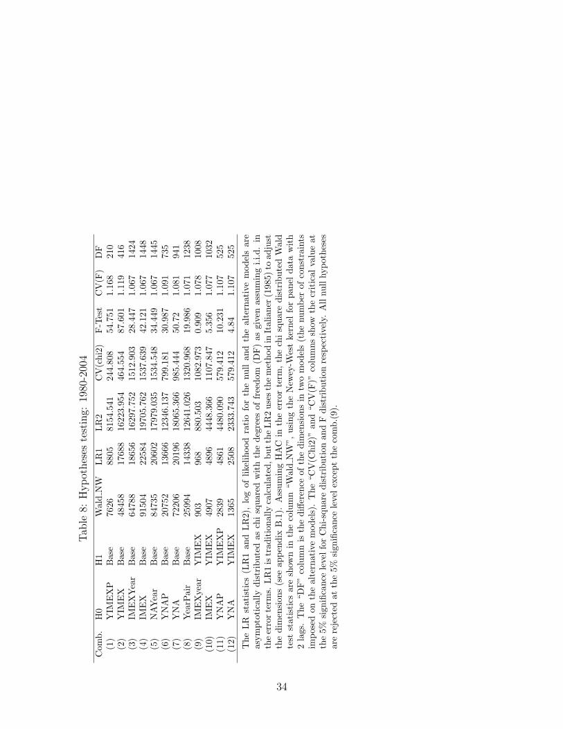
Tab

le8:

Hypotheses

testing:

1980-2004

Com

b.

H0

H1

WaldNW

LR1

LR2

CV(chi2)

F-Test

CV(F

)DF

(1)

YIM

EXP

Base

7626

8805

8154

.541

244.80

854

.751

1.16

821

0(2)

YIM

EX

Base

4845

817

688

1622

3.95

446

4.55

487

.601

1.11

941

6(3)

IMEXYear

Base

6478

818

656

1629

7.75

215

12.903

28.447

1.06

714

24(4)

IMEX

Base

9150

422

584

1970

5.76

215

37.639

42.121

1.06

714

48(5)

NAYear

Base

8473

520

602

1797

9.03

515

34.548

34.449

1.06

714

45(6)

YNAP

Base

2075

213

666

1234

6.13

779

9.18

130

.987

1.09

173

5(7)

YNA

Base

7220

620

196

1806

5.36

698

5.44

450

.72

1.08

194

1(8)

YearP

air

Base

2599

414

338

1264

1.02

613

20.968

19.986

1.07

112

38(9)

IMEXyear

YIM

EX

903

968

880.50

310

82.973

0.90

91.07

810

08(10)

IMEX

YIM

EX

4907

4896

4448

.366

1107

.847

5.35

61.07

710

32(11)

YNAP

YIM

EXP

2839

4861

4480

.090

579.41

210

.231

1.10

752

5(12)

YNA

YIM

EX

1365

2508

2333

.743

579.41

24.84

1.10

752

5

TheLR

statistics

(LR1an

dLR2),logof

likelihoodratioforthenullan

dthealternativemodelsare

asymptoticallydistributedas

chisquared

withthedegrees

offreedom

(DF)as

given

assumingi.i.d.in

theerrorterm

s.LR1istrad

itionally

calculated,buttheLR2usesthemethodin

Italianer

(198

5)to

adjust

thedim

ension

s(see

appen

dix

B.1).

AssumingHAC

intheerrorterm

,thechisquaredistributedWald

test

statistics

areshow

nin

thecolumn“W

aldNW

”,usingtheNew

ey-W

estkernel

forpan

eldatawith

2lags.

The“D

F”columnis

thedifferen

ceof

thedim

ension

sin

twomodels(thenumber

ofconstraints

imposedon

thealternativemodels).The“C

V(C

hi2)”

and“C

V(F

)”columnsshow

thecritical

valueat

the5%

sign

ificance

level

forChi-squaredistribution

andFdistribution

respectively.

Allnullhypotheses

arerejected

atthe5%

sign

ificance

level

exceptthecomb.(9).

34

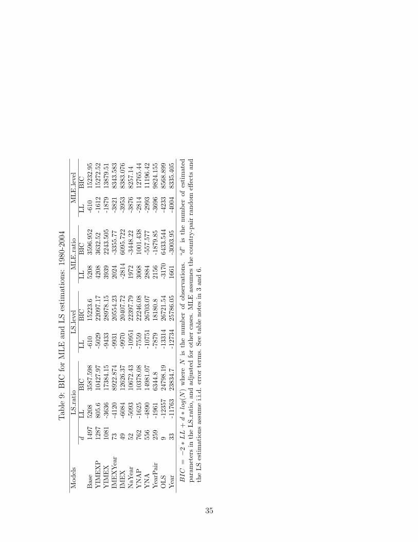
Tab

le9:

BIC

forMLEan

dLSestimations:

1980-2004

Models

LSratio

LSlevel

MLE

ratio

MLE

level

dLL

BIC

LL

BIC

LL

BIC

LL

BIC

Base

1497

5208

3587

.598

-610

1522

3.6

5208

3596

.952

-610

1523

2.95

YIM

EXP

1287

805.6

1042

7.97

-502

922

097.17

4208

3632

.52

-161

215

272.52

YIM

EX

1081

-363

617

384.15

-943

328

978.15

3939

2243

.505

-187

913

879.51

IMEXYear

73-412

089

22.874

-993

120

554.23

2024

-335

5.77

-382

183

43.583

IMEX

49-608

412

626.37

-997

020

407.72

-281

460

95.722

-395

383

83.076

NaY

ear

52-509

310

672.43

-109

5122

397.79

1972

-344

8.22

-387

682

57.14

YNAP

762

-162

510

378.08

-755

922

246.08

3068

1001

.438

-281

412

765.44

YNA

556

-489

014

981.07

-107

5126

703.07

2884

-557

.577

-299

311

196.42

YearP

air

259

-196

163

44.8

-787

918

180.8

2156

-187

9.85

-369

698

24.155

OLS

9-123

5724

798.19

-133

1426

721.54

-317

064

33.544

-423

385

68.899

Year

33-117

6323

834.7

-127

3425

786.05

1661

-300

3.95

-400

483

35.405

BIC

=−2∗LL+

d∗log(N

)whereN

isthenumber

ofob

servations.

“d”is

thenumber

ofestimated

parametersin

theLSratio,

andad

justed

forother

cases.

MLE

assumes

thecountry-pairrandom

effects

and

theLSestimationsassumei.i.d.errorterm

s.See

table

notes

in3an

d6.

35

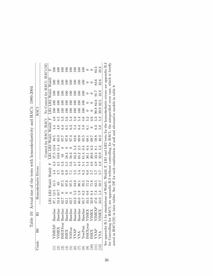
Tab

le10:Actual

size

ofthetestswithhom

oskedasticity

andHAC1:

1980-2004

Com

b.

H0

H1

Hom

osked

asticErrors

HAC1

Con

trol

forHAC1:

HAC1

NoCon

trol

forHAC1:

HAC1(M)

LR1LR2Wald1Wald2

FLR1LR2Wald1Wald2

FLR1LR2Wald1Wald2

F(1)

YIM

EXP

Baseline

37.1

12.5

41.5

4.4

4.3

37.5

13.6

40.5

4.4

4.0

100

100

100

100

100

(2)

YIM

EX

Baseline

53.4

10.7

654.7

4.5

53.6

11.4

65.3

4.8

4.5

100

100

100

100

100

(3)

IMEXYearBaseline

62.7

097

.56.9

5.3

590

97.7

6.4

5.3

100

100

100

100

100

(4)

IMEX

Baseline

62.1

097

.66.9

5.5

58.4

097

.96.5

5.6

100

100

100

100

100

(5)

NAYear

Baseline

62.7

097

.57.1

5.6

58.3

097

.46.3

5.4

100

100

100

100

100

(6)

YNAP

Baseline

63.3

5.2

83.9

5.5

4.7

62.2

5.2

82.6

5.4

5.0

100

100

100

100

100

(7)

YNA

Baseline

66.0

1.9

90.1

5.4

4.3

65.2

2.5

89.9

6.4

5.4

100

100

100

100

100

(8)

YearP

air

Baseline

65.7

0.2

95.5

6.2

5.1

61.4

0.4

95.5

5.9

4.6

100

100

100

100

100

(9)

IMEXyearYIM

EX

33.5

0.6

71.2

6.0

5.3

30.1

0.4

68.1

6.1

5.2

00

00

0(10)

IMEX

YIM

EX

32.9

0.4

71.8

5.7

4.8

30.6

0.3

69.7

64.6

00

00

0(11)

YNAP

YIM

EXP

47.6

7.3

62.5

5.7

4.9

43.4

8.1

59.8

6.3

5.3

90.8

84.6

91.7

83.6

83.3

(12)

YNA

YIM

EX

34.0

5.3

50.7

5.7

4.9

32.9

5.3

48.3

5.6

5.3

39.9

32.5

42.8

32.6

32.3

See

appen

dix

B.1

forsimulation

sof

Wald1,

Wald2,

F,LR1an

dLR2testsforthehom

osked

asticerrors;seeap

pen

dix

B.2

forControllingforHAC1;

seeap

pen

dix

B.3

withou

tcontrollingforHAC1,

themisspecified

errorcase,whichis

briefl

ynoted

asHAC1(M)in

latertables.

See

DFforeach

combinationof

nullan

dalternativemodelsin

table

8.

36

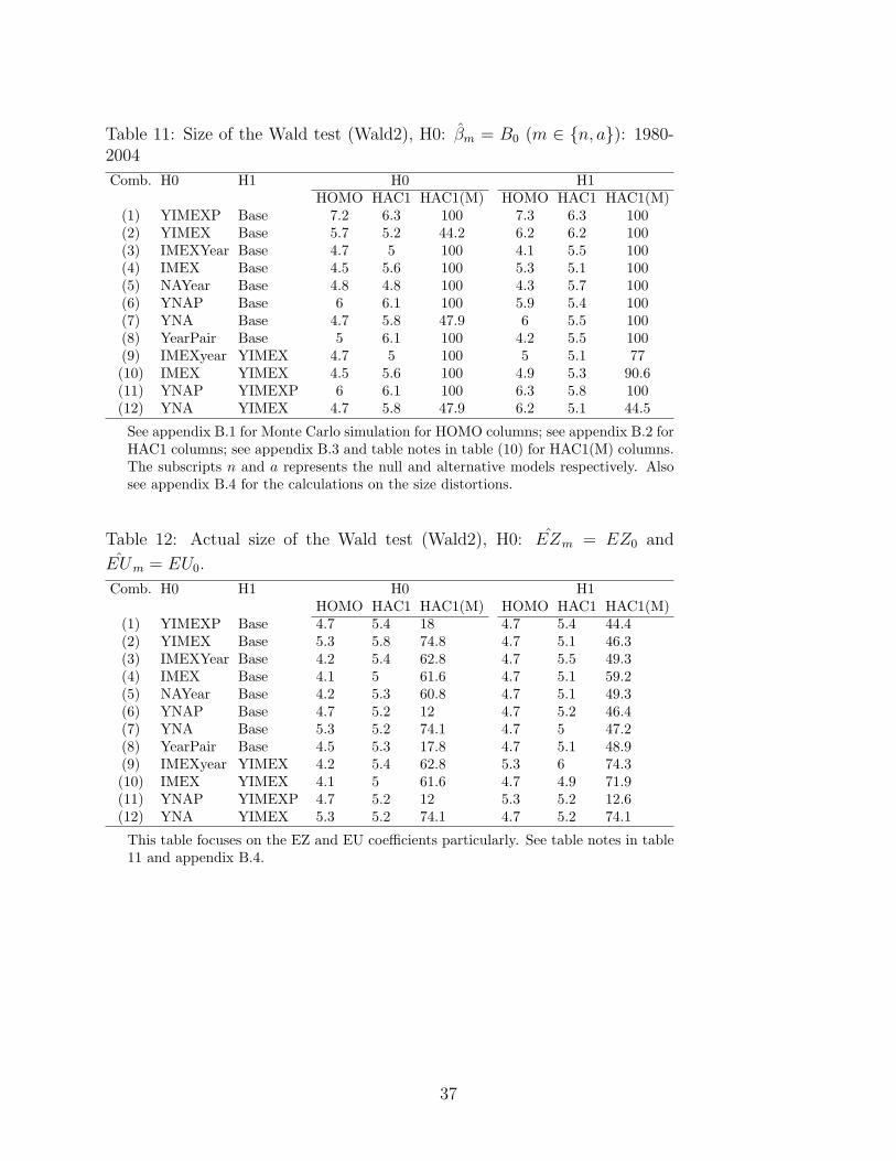
Table 11: Size of the Wald test (Wald2), H0: βm = B0 (m ∈ n, a): 1980-2004

Comb. H0 H1 H0 H1HOMO HAC1 HAC1(M) HOMO HAC1 HAC1(M)

(1) YIMEXP Base 7.2 6.3 100 7.3 6.3 100(2) YIMEX Base 5.7 5.2 44.2 6.2 6.2 100(3) IMEXYear Base 4.7 5 100 4.1 5.5 100(4) IMEX Base 4.5 5.6 100 5.3 5.1 100(5) NAYear Base 4.8 4.8 100 4.3 5.7 100(6) YNAP Base 6 6.1 100 5.9 5.4 100(7) YNA Base 4.7 5.8 47.9 6 5.5 100(8) YearPair Base 5 6.1 100 4.2 5.5 100(9) IMEXyear YIMEX 4.7 5 100 5 5.1 77(10) IMEX YIMEX 4.5 5.6 100 4.9 5.3 90.6(11) YNAP YIMEXP 6 6.1 100 6.3 5.8 100(12) YNA YIMEX 4.7 5.8 47.9 6.2 5.1 44.5

See appendix B.1 for Monte Carlo simulation for HOMO columns; see appendix B.2 forHAC1 columns; see appendix B.3 and table notes in table (10) for HAC1(M) columns.The subscripts n and a represents the null and alternative models respectively. Alsosee appendix B.4 for the calculations on the size distortions.

Table 12: Actual size of the Wald test (Wald2), H0: EZm = EZ0 and

EUm = EU0.

Comb. H0 H1 H0 H1HOMO HAC1 HAC1(M) HOMO HAC1 HAC1(M)

(1) YIMEXP Base 4.7 5.4 18 4.7 5.4 44.4(2) YIMEX Base 5.3 5.8 74.8 4.7 5.1 46.3(3) IMEXYear Base 4.2 5.4 62.8 4.7 5.5 49.3(4) IMEX Base 4.1 5 61.6 4.7 5.1 59.2(5) NAYear Base 4.2 5.3 60.8 4.7 5.1 49.3(6) YNAP Base 4.7 5.2 12 4.7 5.2 46.4(7) YNA Base 5.3 5.2 74.1 4.7 5 47.2(8) YearPair Base 4.5 5.3 17.8 4.7 5.1 48.9(9) IMEXyear YIMEX 4.2 5.4 62.8 5.3 6 74.3(10) IMEX YIMEX 4.1 5 61.6 4.7 4.9 71.9(11) YNAP YIMEXP 4.7 5.2 12 5.3 5.2 12.6(12) YNA YIMEX 5.3 5.2 74.1 4.7 5.2 74.1

This table focuses on the EZ and EU coefficients particularly. See table notes in table11 and appendix B.4.

37

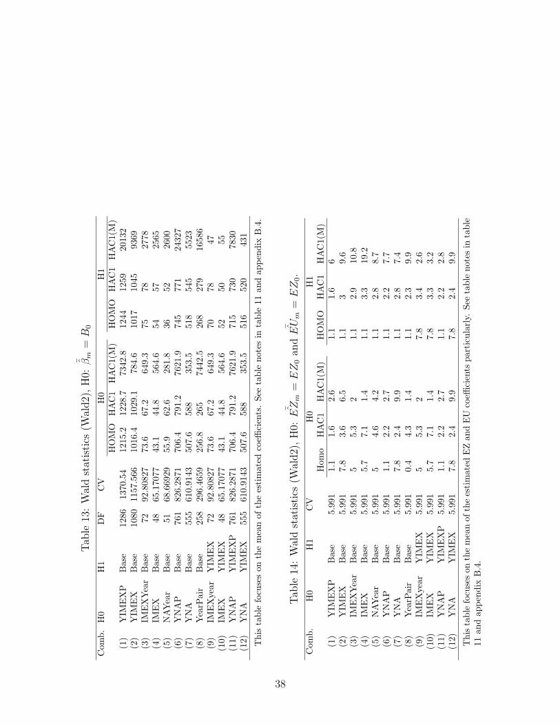
Tab

le13:Waldstatistics

(Wald2),H0:

¯ βm=

B0

Com

b.

H0

H1

DF

CV

H0

H1

HOMO

HAC1

HAC1(M)

HOMO

HAC1

HAC1(M)

(1)

YIM

EXP

Base

1286

1370

.54

1215

.212

28.7

7342

.812

4412

5920

132

(2)

YIM

EX

Base

1080

1157

.566

1016

.410

29.1

784.6

1017

1045

9369

(3)

IMEXYear

Base

7292

.808

2773

.667

.264

9.3

7578

2778

(4)

IMEX

Base

4865

.170

7743

.144

.856

4.6

5457

2565

(5)

NAYear

Base

5168

.669

2955

.962

.628

1.8

3652

2600

(6)

YNAP

Base

761

826.28

7170

6.4

791.2

7621

.974

577

124

327

(7)

YNA

Base

555

610.91

4350

7.6

588

353.5

518

545

5523

(8)

YearP

air

Base

258

296.46

5925

6.8

265

7442

.526

827

916

586

(9)

IMEXyear

YIM

EX

7292

.808

2773

.667

.264

9.3

7078

47(10)

IMEX

YIM

EX

4865

.170

7743

.144

.856

4.6

5250

55(11)

YNAP

YIM

EXP

761

826.28

7170

6.4

791.2

7621

.971

573

078

30(12)

YNA

YIM

EX

555

610.91

4350

7.6

588

353.5

516

520

431

This

table

focu

seson

themeanof

theestimated

coeffi

cients.See

table

notes

intable

11an

dap

pen

dix

B.4.

Tab

le14:Waldstatistics

(Wald2),H0:

¯EZ

m=

EZ

0an

d¯

EUm=

EZ

0.

Com

b.

H0

H1

CV

H0

H1

Hom

oHAC1

HAC1(M)

HOMO

HAC1

HAC1(M)

(1)

YIM

EXP

Base

5.99

11.1

1.6

2.6

1.1

1.6

6(2)

YIM

EX

Base

5.99

17.8

3.6

6.5

1.1

39.6

(3)

IMEXYear

Base

5.99

15

5.3

21.1

2.9

10.8

(4)

IMEX

Base

5.99

15.7

7.1

1.4

1.1

3.3

19.2

(5)

NAYear

Base

5.99

15

4.6

4.2

1.1

2.8

8.7

(6)

YNAP

Base

5.99

11.1

2.2

2.7

1.1

2.2

7.7

(7)

YNA

Base

5.99

17.8

2.4

9.9

1.1

2.8

7.4

(8)

YearP

air

Base

5.99

10.4

4.3

1.4

1.1

2.3

9.9

(9)

IMEXyear

YIM

EX

5.99

15

5.3

27.8

3.4

2.6

(10)

IMEX

YIM

EX

5.99

15.7

7.1

1.4

7.8

3.3

3.2

(11)

YNAP

YIM

EXP

5.99

11.1

2.2

2.7

1.1

2.2

2.8

(12)

YNA

YIM

EX

5.99

17.8

2.4

9.9

7.8

2.4

9.9

Thistable

focu

seson

themeanof

theestimated

EZan

dEU

coeffi

cients

particu

larly.

See

table

notes

intable

11an

dap

pen

dix

B.4.

38

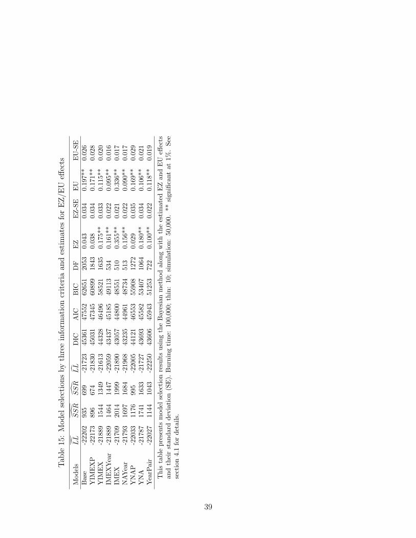
Tab

le15:Model

selectionsbythreeinform

ationcriteria

andestimates

forEZ/E

Ueff

ects

Models

LL

SSR

SSR

LL

DIC

AIC

BIC

DF

EZ

EZ-SE

EU

EU-SE

Base

-222

0293

569

9-217

2345

361

4755

262

651

2053

0.04

30.03

40.19

7**

0.02

6YIM

EXP

-221

7389

667

4-218

3045

031

4734

560

899

1843

0.03

80.03

40.17

1**

0.02

8YIM

EX

-218

8915

4413

49-216

1344

328

4649

658

521

1635

0.17

5**

0.03

30.11

5**

0.02

0IM

EXYear

-218

8914

6414

47-220

5943

437

4518

549

113

534

0.16

1**

0.02

20.09

5**

0.01

6IM

EX

-217

0920

1419

99-218

9043

057

4480

048

551

510

0.35

5**

0.02

10.33

6**

0.01

7NAYear

-217

9316

9716

84-219

6843

235

4496

148

734

513

0.15

6**

0.02

20.09

0**

0.01

7YNAP

-220

3311

7699

5-220

0544

121

4655

355

908

1272

0.02

90.03

50.16

9**

0.02

9YNA

-217

8717

4116

33-217

2743

693

4558

253

407

1064

0.18

0**

0.03

40.10

6**

0.02

1YearP

air

-220

2711

4410

43-222

5043

606

4594

351

253

722

0.10

0**

0.02

20.11

8**

0.01

9

This

table

presents

model

selectionresultsusingtheBayesianmethodalon

gwiththeestimated

EZan

dEU

effects

andtheirstan

darddeviation

(SE).

Burningtime:

100,00

0;thin:10

;simulation

:50

,000

.**

sign

ificantat

1%.See

section4.1fordetails.

39

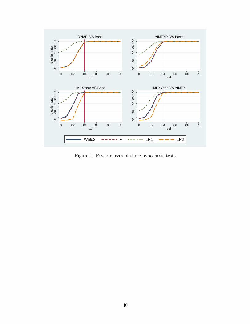
0530

6080

100

reje

ctio

n ra

te

0 .02 .04 .06 .08 .1std

YNAP VS Base

0530

6080

100

0 .02 .04 .06 .08 .1std

YIMEXP VS Base

0530

6080

100

reje

ctio

n ra

te

0 .02 .04 .06 .08 .1std

IMEXYear VS Base

0530

6080

100

0 .02 .04 .06 .08 .1std

IMEXYear VS YIMEX

Wald2 F LR1 LR2

Figure 1: Power curves of three hypothesis tests

40

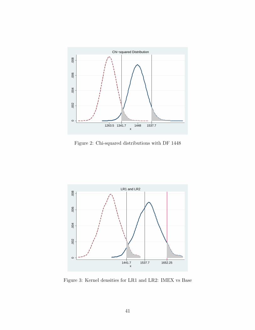
0.0

02.0

04.0

06.0

08

1263.5 1341.7 1448 1537.7x

Chi−squared Distribution

Figure 2: Chi-squared distributions with DF 1448

0.0

02.0

04.0

06.0

08

1441.7 1537.7 1652.25x

LR1 and LR2

Figure 3: Kernel densities for LR1 and LR2: IMEX vs Base

41

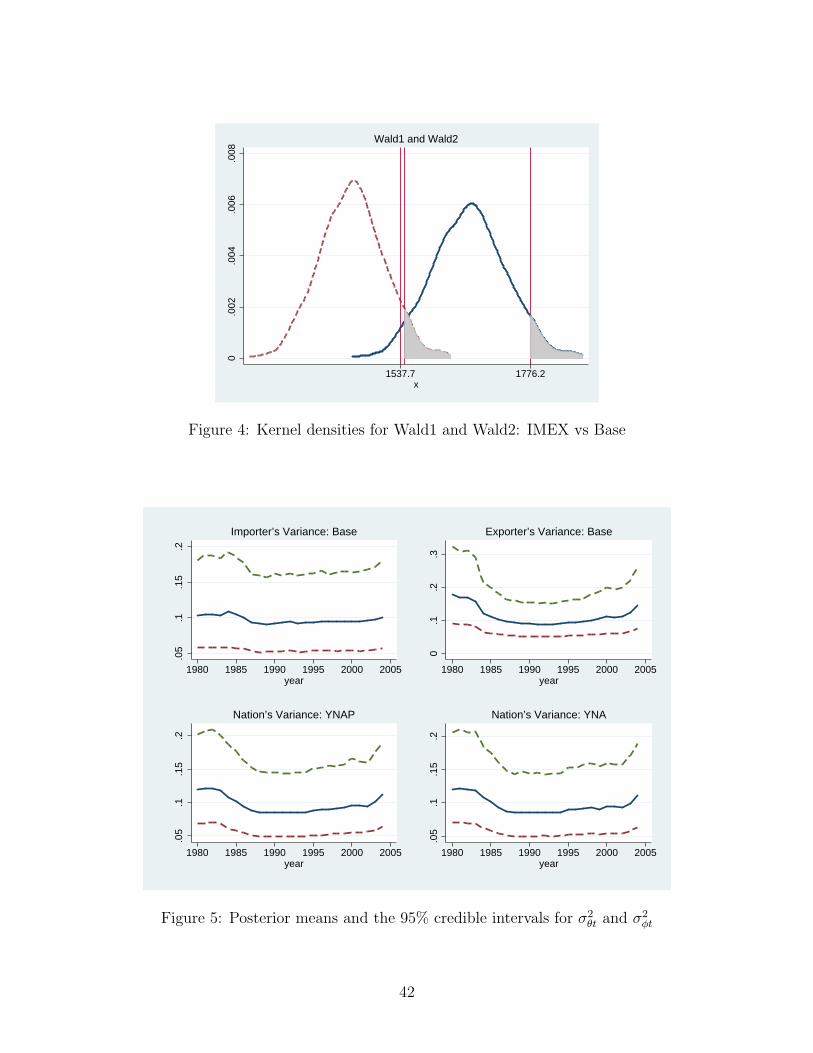
0.0

02.0

04.0

06.0

08

1537.7 1776.2x

Wald1 and Wald2

Figure 4: Kernel densities for Wald1 and Wald2: IMEX vs Base

.05

.1.1

5.2

1980 1985 1990 1995 2000 2005year

Importer’s Variance: Base

0.1

.2.3

1980 1985 1990 1995 2000 2005year

Exporter’s Variance: Base

.05

.1.1

5.2

1980 1985 1990 1995 2000 2005year

Nation’s Variance: YNAP

.05

.1.1

5.2

1980 1985 1990 1995 2000 2005year

Nation’s Variance: YNA

Figure 5: Posterior means and the 95% credible intervals for σ2θt and σ2

ϕt

42