ARTICLE IN PRESS

Volume 88, Issue 1, April 2008ISSN 0304-405X

Managing Editor:Contents lists available at ScienceDirect

JOURNAL OFFinancialECONOMICS

G. WILLIAM SCHWERT

Founding Editor:MICHAEL C. JENSEN

Advisory Editors:EUGENE F. FAMA

KENNETH FRENCHWAYNE MIKKELSON

JAY SHANKENANDREI SHLEIFER

CLIFFORD W. SMITH, JR.RENÉ M. STULZ

Associate Editors:HENDRIK BESSEMBINDER

JOHN CAMPBELLHARRY DeANGELO

DARRELL DUFFIEBENJAMIN ESTY

RICHARD GREENJARRAD HARFORD

PAUL HEALYCHRISTOPHER JAMES

SIMON JOHNSONSTEVEN KAPLANTIM LOUGHRAN

MICHELLE LOWRYKEVIN MURPHYMICAH OFFICERLUBOS PASTORNEIL PEARSON

JAY RITTERRICHARD GREENRICHARD SLOANJEREMY C. STEIN

JERRY WARNERMICHAEL WEISBACH

KAREN WRUCK

Journal of Financial Economics

Journal of Financial Economics 91 (2009) 1–23

0304-40

doi:10.1

$ We

Rosenbe

particip

America

and the

benefite

Andrew� Cor

E-m

edu (R.J

URL

http://w

http://w1 Te2 Te3 Te

Published by ELSEVIERin collaboration with theWILLIAM E. SIMON GRADUATE SCHOOL OF BUSINESS ADMINISTRATION, UNIVERSITY OF ROCHESTER

Available online at www.sciencedirect.com

journal homepage: www.elsevier.com/locate/jfec

High idiosyncratic volatility and low returns: International andfurther U.S. evidence$

Andrew Ang a,1, Robert J. Hodrick b,�, Yuhang Xing c,2, Xiaoyan Zhang d,3

a Columbia Business School, Columbia University and NBER, 3022 Broadway 413 Uris, New York, NY 10027, USAb Columbia Business School, Columbia University and NBER, 3022 Broadway 414 Uris, New York, NY 10027, USAc Jones School of Management, Rice University, Rm 230, MS 531, 6100 Main Street, Houston, TX 77004, USAd Johnson Graduate School of Management, Cornell University, 336 Sage Hall, Ithaca, NY 14850, USA

a r t i c l e i n f o

Article history:

Received 23 January 2006

Received in revised form

9 October 2007

Accepted 18 December 2007Available online 15 October 2008

JEL classification:

F39

G12

Keywords:

Cross-section of stock returns

Predictability

Factor model

5X/$ - see front matter & 2008 Elsevier B.V.

016/j.jfineco.2007.12.005

thank Tobias Adrian, Kewei Hou, Soeren Hv

rg for kindly providing data. We thank Tim Jo

ants at the CRSP Forum at the Universit

n Finance Association, Columbia University

University of Toronto for helpful commen

d from the excellent comments of an a

Ang acknowledges support from the NSF.

responding author. Tel.: +1212 854 3413.

ail addresses: aa610@columbia.edu (A. Ang), r

. Hodrick), yxing@rice.edu (Y. Xing), xz69@cor

S: http://www.columbia.edu/�aa610 (A. Ang)

ww.columbia.edu/�rh169 (R.J. Hodrick),

ww.johnson.cornell.edu/faculty/pro-files/xZh

l.: +1212 854 9154.

l.: +1713 348 4167.

l.: +1607 255 8729.

a b s t r a c t

Stocks with recent past high idiosyncratic volatility have low future average returns

around the world. Across 23 developed markets, the difference in average returns

between the extreme quintile portfolios sorted on idiosyncratic volatility is �1:31% per

month, after controlling for world market, size, and value factors. The effect is

individually significant in each G7 country. In the United States, we rule out

explanations based on trading frictions, information dissemination, and higher

moments. There is strong covariation in the low returns to high-idiosyncratic-volatility

stocks across countries, suggesting that broad, not easily diversifiable factors lie behind

this phenomenon.

& 2008 Elsevier B.V. All rights reserved.

1. Introduction

In a recent paper, Ang, Hodrick, Xing, and Zhang (2006)(AHXZ hereafter) show that volatility of the market return

All rights reserved.

idjkaer, and Joshua

hnson and seminar

y of Chicago, the

, NYU, SAC Capital,

ts. The paper has

nonymous referee.

h169@columbia.

nell.edu (X. Zhang).

,

ang/ (X. Zhang).

is a priced cross-sectional risk factor. After demonstratingthis fact, AHXZ sort firms on the basis of their idiosyn-cratic stock return volatility, measured relative to theFama and French (1993) model. They reason that theidiosyncratic errors of a misspecified factor model couldcontain the influence of missing factors, and hence, bysorting on idiosyncratic volatility, they might develop aset of portfolios that would be mispriced by the Fama andFrench (1993) model but that might be correctly priced bythe new aggregate volatility risk factor. AHXZ find thatU.S. stocks with high lagged idiosyncratic volatility earnvery low future average returns, and these assets areindeed mispriced by the Fama-French model.

The AHXZ results are surprising for two reasons. First,the difference in average returns across stocks with lowand high idiosyncratic volatility is large. In particular, theaverage return on the first quintile portfolio of stocks withthe lowest idiosyncratic volatility exceeds the averagereturn on the fifth quintile portfolio of stocks with the

ARTICLE IN PRESS

2 According to an ICAPM, a factor which predicts stock returns in the

cross section should also predict aggregate market returns (see Campbell,

A. Ang et al. / Journal of Financial Economics 91 (2009) 1–232

highest idiosyncratic volatility by over 1% per month.Second, AHXZ demonstrate that their findings cannot beexplained either by exposure to aggregate volatility risk orby other existing asset pricing models. AHXZ’s findings areparticularly puzzling for financial theories that linkidiosyncratic volatility to expected returns. While idiosyn-cratic volatility is not priced in a correctly specified factormodel, in environments with frictions and incompleteinformation the idiosyncratic volatility of a stock may belinked to its expected return. For example, Merton (1987)shows that in the presence of market frictions whereinvestors have limited access to information, stocks withhigh idiosyncratic volatility have high expected returnsbecause investors cannot fully diversify away firm-specificrisk. But AHXZ find the exact opposite relation.

This paper contains three main contributions. Our firstgoal is to see if the anomalous relation between laggedidiosyncratic volatility and future average returns in U.S.data exists in other markets. As with any empirical results,there is a danger that AHXZ’s finding is dependent only ona particular small sample. AHXZ’s results could bedatasnooping, as argued by Lo and MacKinlay (1990).1 Ifa relation between lagged idiosyncratic volatility andfuture average returns exists in international markets, it ismore likely that there is an underlying economic sourcebehind the phenomenon. Thus, we examine whether stockreturns in international markets sorted on idiosyncraticvolatility conform to the same pattern observed in the U.S.cross section.

We present evidence that the negative relation be-tween lagged idiosyncratic volatility and future averagereturns is observed across a broad sample of internationaldeveloped markets. In particular, for each of the largestseven (G7) equity markets (Canada, France, Germany,Italy, Japan, the United States, and the United Kingdom),stocks with high idiosyncratic volatility tend to have lowaverage returns. The negative idiosyncratic volatility–average return relation is strongly statistically significantin each of these countries and is also observed in thelarger sample of 23 developed markets. From these stronginternational results, it is hard to explain the low returnsto high-idiosyncratic-volatility stocks as a small-sampleproblem.

Our second, and perhaps most interesting, contributionis that the negative spread in returns between stocks withhigh and low idiosyncratic volatility in internationalmarkets strongly co-moves with the difference in returnsbetween U.S. stocks with high and low idiosyncraticvolatilities. The large commonality in co-movementshared by the spread in returns between stocks with highand low idiosyncratic volatility across countries suggeststhat broad, not easily diversifiable factors lie behind thiseffect. However, we do not claim that the low averagereturns to stocks with high idiosyncratic volatility repre-sent a priced risk factor because we do not yet have atheoretical framework to understand why agents have

1 AHXZ’s results could also have just been wrong, but the AHXZ

results for U.S. stocks have been independently confirmed by Brown and

Ferreira (2003), Jiang, Xu, and Yao (2005), Huang, Liu, Rhee, and Zhang

(2006), Zhang (2006), and Bali and Cakici (2008).

high demand for high-idiosyncratic-volatility stocks,causing these stocks to have low expected returns.

Finally, in detailed analysis of the U.S. market wheremore data are available, we rule out explanations based onmarket frictions, information dissemination, and optionpricing. We consider the effects of transaction costs byusing the incidence of zero returns proposed by Lesmond,Ogden, and Trzcinka (1999). To characterize the severity ofmarket frictions, we control for Hou and Moskowitz’s(2005) delay with which a stock’s price responds toinformation. Since the extent of analyst coverage andinstitutional ownership are important determinants fortrading volume (Chordia, Huh, and Subrahmanyam, 2007)and can proxy for the proportion of informed agents(Brennan and Subrahmanyam, 1995), we investigatewhether the idiosyncratic volatility effect persists aftercontrolling for both of these variables. We also investigatethe relation to the amount of private information intrading activity (Easley, Hvidkjaer, and O’Hara, 2002) andto skewness (Barberis and Huang, 2005). An alternativeexplanation suggested by Johnson (2004) is that theidiosyncratic volatility effect is due to idiosyncraticvolatility interacting with leverage, motivated from thefact that equity is a call option on a firm’s underlyingassets. None of these explanations can entirely account forthe high idiosyncratic volatility and low average returnsrelation.

In our analysis, we investigate the relation betweenfuture returns and past idiosyncratic volatility. Thus, theidiosyncratic volatility effect that we document in bothU.S. and international markets is not necessarily a relationthat involves expected volatility (Fu, 2005; Spiegel andWang, 2005), which is unobservable and must beestimated. In contrast, past idiosyncratic volatility is anobservable, easily calculated stock characteristic. Sinceidiosyncratic volatility is persistent, we expect that ourlagged measure is correlated with future idiosyncraticvolatility that agents might assess in determining ex-pected returns. Thus, we also examine the contempora-neous relation between expected future idiosyncraticvolatility and realized returns. Our investigation indicatesthat a strong negative relation between lagged idiosyn-cratic volatility and future returns remains even aftercontrolling for the information that past idiosyncraticvolatility provides about future idiosyncratic volatility.

Our results are related to a literature that investigateswhether idiosyncratic volatility can predict future aggre-gate market returns (see, e.g., Goyal and Santa-Clara,2003; Bali et al., 2005; Wei and Zhang, 2005; Guo andSavickas, 2007). Goyal and Santa-Clara (2003) findthat average idiosyncratic volatility predicts aggregatemarket excess returns.2 However, our focus is on the

1993). However, if returns are tied to firm characteristics rather than

factor loadings as advocated by Daniel and Titman (1997), then because

idiosyncratic volatility is a firm characteristic, a relation between

idiosyncratic volatility and returns at the firm level does not imply a

relation between average idiosyncratic volatility and market returns at

the aggregate level.

ARTICLE IN PRESS

A. Ang et al. / Journal of Financial Economics 91 (2009) 1–23 3

cross-sectional, as opposed to the aggregate time series,relation between firm-level idiosyncratic volatility andexpected returns. Other authors, like Campbell, Lettau,Malkiel, and Xu (2001), Bekaert, Hodrick, and Zhang(2005), and Brandt, Brav, and Graham (2005) haveexamined trends in average idiosyncratic volatility, butthey do not link idiosyncratic volatility to cross-sectionalreturns.

Idiosyncratic volatility has been used to proxy forvarious economic effects. For example, building on Miller(1977), idiosyncratic volatility has been used as aninstrument to measure differences in opinion (see, e.g.,Baker, Coval, and Stein, 2007). We do not investigate thesuccess of idiosyncratic volatility to proxy for differenteconomic effects, and AHXZ show that differences inopinion measured by analyst dispersion (see Diether,Malloy, and Scherbina, 2002) cannot account for theidiosyncratic volatility effect. Our focus is on howidiosyncratic volatility itself is related to expected returnsin the cross-section of international stock returns. Simi-larly, idiosyncratic volatility could be related to othereconomic factors, like liquidity risk (see, e.g., Spiegel andWang, 2005). Hence, we specifically control for the effectof other risk loadings or risk characteristics in our analysisof idiosyncratic volatility.

The remainder of the paper is organized as follows.Section 2 describes how we measure the idiosyncraticvolatility of a stock and discusses the international stockreturn data. Section 3 explains our cross-sectional versionof the Fama and MacBeth (1973) methodology. Section 4shows that the negative relation between idiosyncraticvolatility and future returns is observed across the world,while Section 5 examines how the difference in returnsbetween foreign stocks with high and low idiosyncraticvolatilities covaries with the analogous difference in U.S.stock returns. In Section 6, we examine in detail somepotential economic explanations for the effect using U.S.data. We rule out market frictions, asymmetric informa-tion, skewness, and an interaction with leverage ascomplete explanations for the idiosyncratic volatilityphenomenon. Section 7 concludes.

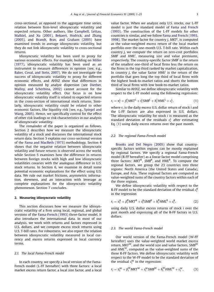
2. Measuring idiosyncratic volatility

This section discusses how we measure the idiosyn-cratic volatility of a firm using local, regional, and globalversions of the Fama-French (1993) three-factor model. Italso introduces the international data. In most of ouranalysis, we work with returns and factors expressed inU.S. dollars, and we compute excess stock returns usingU.S. T-bill rates. For robustness, we also report the relationbetween idiosyncratic volatility measured in local cur-rency and excess returns expressed in local currencyterms.

2.1. The local Fama-French model

In each country, we specify a local version of the Fama-French model (L-FF hereafter) with three factors: a localmarket excess return factor, a local size factor, and a local

value factor. When we analyze only U.S. stocks, our L-FFmodel is just the standard model of Fama and French(1993). The construction of the L-FF models for othercountries is similar, and we follow Fama and French (1993,1998). The market factor for country j, MKTj, is computedas the value-weighted excess return of the local marketportfolio over the one-month U.S. T-bill rate. Within eachcountry j, we compute the return on zero-cost portfoliosSMBj and HMLj, measuring size and value premiums,respectively. The country-specific factor SMBj is the returnof the smallest one-third of local firms less the return onthe firms in the top third ranked by market capitalization.In country j, the value factor HMLj is the return of theportfolio that goes long the top third of local firms withthe highest book-to-market ratios and shorts the bottomthird of local firms with low book-to-market ratios.

Similar to AHXZ, we define idiosyncratic volatility withrespect to the L-FF model using the following regression:

ri ¼ aLi þ bL

i MKTLþ sL

i SMBLþ hL

i HMLLþ eL

i , (1)

where ri is the daily excess U.S. dollar return of stock i andthe L-FF factors are also expressed in U.S. dollars.The idiosyncratic volatility for stock i is measured as thestandard deviation of the residuals eL

i after estimatingEq. (1) using daily excess returns over the past month.

2.2. The regional Fama-French model

Brooks and Del Negro (2005) show that country-specific factors within regions can be mostly explainedby regional factors. We specify a regional Fama-Frenchmodel (R-FF hereafter) as a linear factor model comprisingthree factors: MKTR, SMBR, and HMLR. To compute theregional factors, we group the 23 countries into threeregions: North America (the United States and Canada),Europe, and Asia. These regional factors are computed asvalue-weighted sums of the country factors within each ofthe three regions.

We define idiosyncratic volatility with respect to theR-FF model to be the standard deviation of the residual eR

i

in the regression

ri ¼ aRi þ bR

i MKTRþ sR

i SMBRþ hR

i HMLRþ eR

i , (2)

using daily U.S. dollar excess returns of stock i over thepast month and expressing all of the R-FF factors in U.S.dollars.

2.3. The world Fama-French model

Our world version of the Fama-French model (W-FFhereafter) uses the value-weighted world market excessreturn, MKTW, and the world size and value factors, SMBW

and HMLW, computed as the value-weighted sums of thethree R-FF factors. We define idiosyncratic volatility withrespect to the W-FF model to be the standard deviation ofthe residual eW

i in the regression:

ri ¼ aWi þ bW

i MKTWþ sW

i SMBWþ hW

i HMLWþ eW

i , (3)

ARTICLE IN PRESS

A. Ang et al. / Journal of Financial Economics 91 (2009) 1–234

using daily U.S. dollar excess returns of stock i over thepast month and expressing all of the W-FF factors in U.S.dollars.

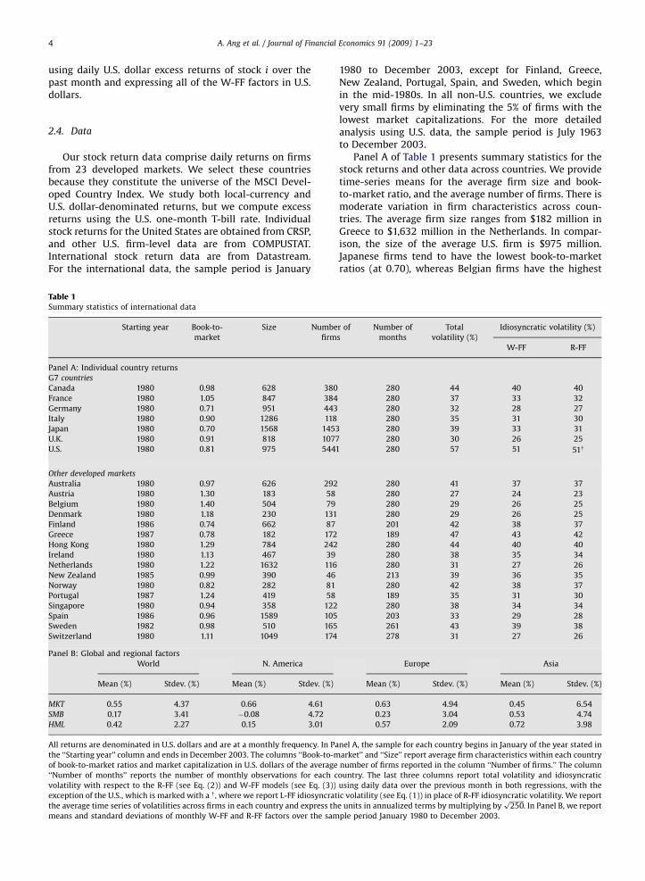
2.4. Data

Our stock return data comprise daily returns on firmsfrom 23 developed markets. We select these countriesbecause they constitute the universe of the MSCI Devel-oped Country Index. We study both local-currency andU.S. dollar-denominated returns, but we compute excessreturns using the U.S. one-month T-bill rate. Individualstock returns for the United States are obtained from CRSP,and other U.S. firm-level data are from COMPUSTAT.International stock return data are from Datastream.For the international data, the sample period is January

Table 1Summary statistics of international data

Starting year Book-to-

market

Size Numbe

firm

Panel A: Individual country returns

G7 countries

Canada 1980 0.98 628 380

France 1980 1.05 847 384

Germany 1980 0.71 951 443

Italy 1980 0.90 1286 118

Japan 1980 0.70 1568 1453

U.K. 1980 0.91 818 1077

U.S. 1980 0.81 975 5441

Other developed markets

Australia 1980 0.97 626 292

Austria 1980 1.30 183 58

Belgium 1980 1.40 504 79

Denmark 1980 1.18 230 131

Finland 1986 0.74 662 87

Greece 1987 0.78 182 172

Hong Kong 1980 1.29 784 242

Ireland 1980 1.13 467 39

Netherlands 1980 1.22 1632 116

New Zealand 1985 0.99 390 46

Norway 1980 0.82 282 81

Portugal 1987 1.24 419 58

Singapore 1980 0.94 358 122

Spain 1986 0.96 1589 105

Sweden 1982 0.98 510 165

Switzerland 1980 1.11 1049 174

Panel B: Global and regional factors

World N. America

Mean (%) Stdev. (%) Mean (%) Stdev. (%)

MKT 0.55 4.37 0.66 4.61

SMB 0.17 3.41 �0.08 4.72

HML 0.42 2.27 0.15 3.01

All returns are denominated in U.S. dollars and are at a monthly frequency. In Pa

the ‘‘Starting year’’ column and ends in December 2003. The columns ‘‘Book-to-m

of book-to-market ratios and market capitalization in U.S. dollars of the average

‘‘Number of months’’ reports the number of monthly observations for each c

volatility with respect to the R-FF (see Eq. (2)) and W-FF models (see Eq. (3))

exception of the U.S., which is marked with a y , where we report L-FF idiosyncrat

the average time series of volatilities across firms in each country and express th

means and standard deviations of monthly W-FF and R-FF factors over the sam

1980 to December 2003, except for Finland, Greece,New Zealand, Portugal, Spain, and Sweden, which beginin the mid-1980s. In all non-U.S. countries, we excludevery small firms by eliminating the 5% of firms with thelowest market capitalizations. For the more detailedanalysis using U.S. data, the sample period is July 1963to December 2003.

Panel A of Table 1 presents summary statistics for thestock returns and other data across countries. We providetime-series means for the average firm size and book-to-market ratio, and the average number of firms. There ismoderate variation in firm characteristics across coun-tries. The average firm size ranges from $182 million inGreece to $1,632 million in the Netherlands. In compar-ison, the size of the average U.S. firm is $975 million.Japanese firms tend to have the lowest book-to-marketratios (at 0.70), whereas Belgian firms have the highest

r of

s

Number of

months

Total

volatility (%)

Idiosyncratic volatility (%)

W-FF R-FF

280 44 40 40

280 37 33 32

280 32 28 27

280 35 31 30

280 39 33 31

280 30 26 25

280 57 51 51y

280 41 37 37

280 27 24 23

280 29 26 25

280 29 26 25

201 42 38 37

189 47 43 42

280 44 40 40

280 38 35 34

280 31 27 26

213 39 36 35

280 42 38 37

189 35 31 30

280 38 34 34

203 33 29 28

261 43 39 38

278 31 27 26

Europe Asia

Mean (%) Stdev. (%) Mean (%) Stdev. (%)

0.63 4.94 0.45 6.54

0.23 3.04 0.53 4.74

0.57 2.09 0.72 3.98

nel A, the sample for each country begins in January of the year stated in

arket’’ and ‘‘Size’’ report average firm characteristics within each country

number of firms reported in the column ‘‘Number of firms.’’ The column

ountry. The last three columns report total volatility and idiosyncratic

using daily data over the previous month in both regressions, with the

ic volatility (see Eq. (1)) in place of R-FF idiosyncratic volatility. We report

e units in annualized terms by multiplying byffiffiffiffiffiffiffiffiffi

250p

. In Panel B, we report

ple period January 1980 to December 2003.

ARTICLE IN PRESS

A. Ang et al. / Journal of Financial Economics 91 (2009) 1–23 5

(at 1.40). Note that the average number of U.S. firms, 5,441,dwarfs the number of firms in any other market. The nextlargest equity market is Japan, which has an average of1,453 firms. Because of the dominant number of U.S. firms,we are careful in our empirical work to disentangle theeffect of the U.S. on any result involving data pooled acrossmarkets.

In Panel A, we report summary statistics for threedifferent average volatility measures, which are allannualized by multiplying by

ffiffiffiffiffiffiffiffiffi

250p

. The first measure istotal volatility, which is computed as the volatility of dailyraw returns over the previous month. The second andthird measures are idiosyncratic volatility computed withrespect to the R-FF model (Eq. (2)) and the W-FF model(Eq. (3)). All three volatility measures are highly corre-lated with each other, with the correlations all above 95%in each country. The United Kingdom has the lowestidiosyncratic volatility (26% per annum with respect toW-FF), compared to the average W-FF idiosyncraticvolatility across countries of 41% per annum. There is alsoquite a wide range in the dispersion of idiosyncraticvolatility across markets. For the United States, theinterquartile range (the difference between the 75thand 25th percentiles) of W-FF idiosyncratic volatility is61:1%� 25:0% ¼ 36:1%, compared to an average inter-quartile range of 38:4%� 18:5% ¼ 19:9% for the other22 countries. Stock-level volatility is only weakly corre-lated with aggregate volatility in each country. In theUnited States, the average correlation of L-FF idiosyncraticvolatility with aggregate market volatility using monthlydata, where both measures are computed using dailyreturns over the month, is only 16.5%. While Campbell,Lettau, Malkiel, and Xu (2001) report a time trend inidiosyncratic volatility over the late 1990s, Brandt, Brav,and Graham (2005) report that there is no time trendextending the sample into the 2000s. Bekaert, Hodrick,and Zhang (2005) find similar results in internationalmarkets.

In Panel B of Table 1, we report monthly means andstandard deviations of R-FF and W-FF factors, all ex-pressed in U.S. dollars. The mean of the SMB factor forNorth America is slightly negative, at �0:08% per month,indicating that small firms have not outperformed largefirms in the United States over the post-1980 sample, incontrast to the results first reported by Banz (1981). Theevidence for the size effect is stronger in the post-1980sample for Europe and Asia, where the regional SMB

factors have positive means. Value strategies have alsoperformed better in overseas markets than in the UnitedStates, with high book-to-market stocks significantlyunderperforming low book-to-market stocks during thelate 1990s bull market in the United States. The valuepremium is particularly strong in Asia, where the meanregional HML factor is 0.72% per month. In comparison,the mean of the world HML factor is 0.42% per month.

3. The cross-sectional regression methodology

We examine the relation between total volatility andidiosyncratic volatility with respect to the L-FF, R-FF,

and W-FF models using a series of two-stage Fama andMacBeth (1973) regressions. In the first stage, for everymonth, we regress the cross-sectional firm excess returnsonto idiosyncratic volatility together with various riskfactor loadings, some firm characteristics, and othercontrol variables. In the second stage, we use the timeseries of the regression coefficients and test whether theaverage coefficient on the lagged idiosyncratic volatilitymeasure is significantly different from zero. To take intoaccount serial correlation in the coefficient estimates, wecompute Newey-West (1987) standard errors with fourlags in the second stage.

The Fama-MacBeth cross-sectional regressions take theform

riðt; t þ 1Þ ¼ c þ gsiðt � 1; tÞ þ l0bbiðt; t þ 1Þ þ l0zziðtÞ

þ eiðt þ 1Þ, (4)

where riðt; t þ 1Þ is stock i’s excess return from month t tot þ 1, siðt � 1; tÞ is stock i’s idiosyncratic volatility com-puted using daily data over the previous month from t � 1to t, biðt; t þ 1Þ is a vector of risk factor loadings over themonth t to t þ 1, and ziðtÞ is a vector of firm characteristicsobservable at time t. We use the notation ðt � 1; tÞ andðt; t þ 1Þ to emphasize the timing of the statistics that arecomputed using data from month t � 1 to t and overmonth t to t þ 1, respectively. The cross-sectional regres-sions for a particular country and month use all availablefirm-level data for that country and month.

We are especially interested in the coefficient g onidiosyncratic volatility, which should be zero under thenull hypothesis of a correctly specified factor model. Eachmonth, we run the regression in Eq. (4) with returnsmeasured in percentage terms and use annualizedvolatility numbers as dependent variables. Because ourvolatility measures are known at the beginning of themonth, siðt � 1; tÞ is a measurable statistic at time t.Following Shanken (1992), Eq. (4) controls for exposuresto risk factors by including contemporaneous factorloadings estimated over the current month, biðt; t þ 1Þ,but we obtain almost identical results if we use past factorloadings, biðt � 1; tÞ. These results are available uponrequest.

We use contemporaneous factor loadings because afactor model explains high average returns over a timeperiod with contemporaneous high covariation in factorexposure over the same period if the factor commands apositive risk premium. Using contemporaneous factorloadings is similar to the Fama-MacBeth regressions runby Black, Jensen, and Scholes (1972), Fama and French(1992), and Jagannathan and Wang (1996), among others.We use firm factor loadings from the W-FF model usingMKTW, SMBW, and HMLW as factors, where the W-FFregression (3) is run using daily returns over the monthfrom t to t þ 1. For the United States, we also considercontemporaneous L-FF factor loadings from Eq. (1)computed using daily data over the month from t to t þ 1.

Daniel and Titman (1997) report that factor loadingsmight not account for all variation in expected returnscompared to firm-level characteristics. Hence, we alsoinclude other firm characteristics in the vector ziðtÞ in the

ARTICLE IN PRESS

A. Ang et al. / Journal of Financial Economics 91 (2009) 1–236

Fama-MacBeth regression. All of these characteristics areknown at time t. The firm characteristics include log size,book-to-market ratios, and a Jegadeesh and Titman (1993)momentum characteristic measured by lagged returnsover the previous six months. All of these firm character-istics are measured in U.S. dollars. We also includecountry-specific dummies as fixed effects.

We investigate the relation between idiosyncraticvolatility and expected returns by examining the signand statistical significance of the mean value of g, thecoefficient on the volatility statistic in Eq. (4). Anotherapproach taken by AHXZ to measure the relation betweenaverage returns and idiosyncratic volatility is to formportfolios ranked on idiosyncratic volatility and thenexamine holding-period returns of these portfolios. AHXZconsider controlling for other effects using a series ofdouble-sorted portfolios, but they do not consider Fama-MacBeth regressions.

While the Fama-MacBeth regressions capture variationin cross-sectional expected returns, residual variation andcomponents of returns related to other factors also enterportfolio returns. One advantage of cross-sectional regres-sions is that they allow for controls for multiple factorloadings and characteristics in a setting that retainspower, whereas creating portfolios that have dispersionon more than two dimensions generally results in someportfolios with only a few stocks and, consequently a lot ofnoise. This is especially true for countries with only asmall number of listed stocks. In our analysis of portfolioreturns, we will form portfolios aggregated across geo-graphic areas to ensure that we have a reasonable numberof stocks in our portfolios.

4. Idiosyncratic volatility and expected returns ininternational markets

We begin our analysis by examining the relationbetween lagged idiosyncratic volatility and future stockreturns across the world. Section 4.1 examines the G7countries in detail, while Section 4.2 considers all 23countries.

4.1. Firms in large, developed countries

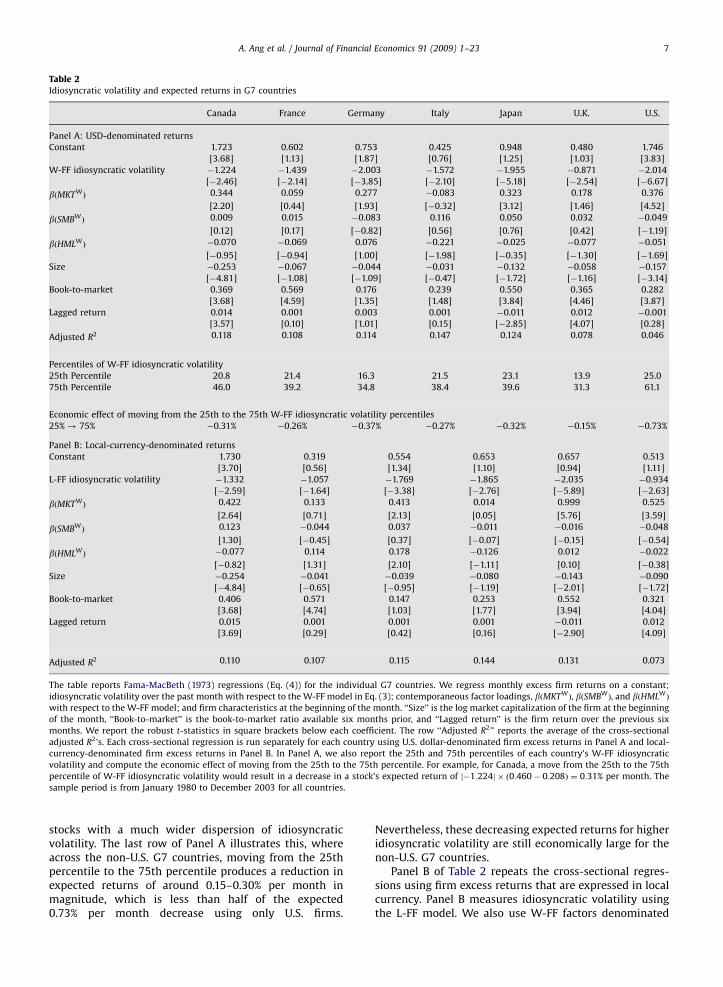
Table 2 reports results of the Fama-MacBeth (1973)regressions in Eq. (4) using stock returns within each ofthe G7 countries. The regressions in Panel A of Table 2 useexcess stock returns denominated in U.S. dollars. Panel Brepeats the cross-sectional regressions using local-currency-denominated excess returns. All regressions arerun using monthly data. Because of data requirements onlagged firm characteristics, the dependent variable returnsof the regressions span September 1980 to December2003, but data on the independent variables, particularlybook values and past returns, begin from January 1980.

The first result in Table 2 is that a strong negativerelation between lagged idiosyncratic volatility andaverage future excess returns exists in each of the non-U.S. G7 countries. For the United States, the estimatedcoefficient on W-FF idiosyncratic volatility is �2:01, with

a robust t-statistic of �6:67. After the United States, thenegative lagged idiosyncratic volatility–expected returnrelation is statistically strongest for Japan, which has apoint estimate of �1:96 with a robust t-statistic of �5:18.The coefficient on W-FF idiosyncratic volatility rangesfrom �0:87 for the United Kingdom to less than �2:00 forGermany. In all cases, the coefficients are statisticallysignificant at the 95% level, with the smallest magnitudeof the t-statistic of �2:10 occurring for Italy.

Second, in contrast to the strong predictive power oflagged idiosyncratic volatility, the coefficients on factorloadings and characteristics are often insignificant. In fact,Table 2 shows that two of the coefficients on SMBW havethe wrong sign from those predicted by Fama and French(1993). This is partly because the small-stock effect andthe value premium in the post-1980 sample are relativelyweak, and possibly because betas contain significantmeasurement error. The book-to-market and laggedreturn characteristics generally have greater statisticalsignificance than the coefficients on the factor betas,consistent with the findings of Daniel and Titman (1997).Examining the coefficients on the characteristics,we find is a statistically significant size effect in Canadaand the United States, and five of the seven book-to-market effects are statistically significant. The relativelyweak evidence of momentum in international stockreturns presumably arises because we take relativelylarge firms for which the momentum effect is weakercompared to small firms (see Rouwenhorst, 1998; Hong,Lim, and Stein, 2000).

To interpret the magnitude of the coefficient onvolatility, we measure the cross-sectional distribution ofvolatility. Panel A of Table 2 reports the 25th percentileand the 75th percentile of W-FF idiosyncratic volatility ineach country. Using these percentiles, we can translate thecoefficients on L-FF idiosyncratic volatility into an eco-nomic effect by asking the following question: if a firmwere to move from the 25th to the 75th idiosyncraticvolatility percentile while its other characteristics wereheld constant, what is the predicted decrease in that firm’sexpected return? The U.S. coefficient of �2:01 translates toa decrease in expected returns of j � 2:01j � ð0:611�0:250Þ ¼ 0:73% per month. These are economically verylarge differences in average excess returns. Of course, thisincrease in idiosyncratic volatility is large, and news thatcaused such a change would probably also be associatedwith changes in other firm characteristics.

While the German and Japanese coefficients onidiosyncratic volatility of �2:00 and �1:96 are similar tothe �2:01 coefficient for the United States, the range ofidiosyncratic volatility in the United States is much largerthan in the other large, developed countries. This makesthe idiosyncratic volatility effect stronger in the UnitedStates, but it still remains large in economic terms for theother countries. The interquartile range of W-FF idiosyn-cratic volatility for the non-U.S. G7 countries is around0.19, which is about half the average interquartile range inthe United States of 0.36. Thus, although the coefficientson W-FF idiosyncratic volatility are similar, the magnitudeof the idiosyncratic volatility effect is approximately halfof the U.S. effect because the United States tends to have

ARTICLE IN PRESS

Table 2Idiosyncratic volatility and expected returns in G7 countries

Canada France Germany Italy Japan U.K. U.S.

Panel A: USD-denominated returns

Constant 1.723 0.602 0.753 0.425 0.948 0.480 1.746

[3.68] [1.13] [1.87] [0.76] [1.25] [1.03] [3.83]

W-FF idiosyncratic volatility �1.224 �1.439 �2.003 �1.572 �1.955 �0.871 �2.014

[�2.46] [�2.14] [�3.85] [�2.10] [�5.18] [�2.54] [�6.67]

bðMKTWÞ 0.344 0.059 0.277 �0.083 0.323 0.178 0.376

[2.20] [0.44] [1.93] [�0.32] [3.12] [1.46] [4.52]

bðSMBWÞ 0.009 0.015 �0.083 0.116 0.050 0.032 �0.049

[0.12] [0.17] [�0.82] [0.56] [0.76] [0.42] [�1.19]

bðHMLWÞ �0.070 �0.069 0.076 �0.221 �0.025 �0.077 �0.051

[�0.95] [�0.94] [1.00] [�1.98] [�0.35] [�1.30] [�1.69]

Size �0.253 �0.067 �0.044 �0.031 �0.132 �0.058 �0.157

[�4.81] [�1.08] [�1.09] [�0.47] [�1.72] [�1.16] [�3.14]

Book-to-market 0.369 0.569 0.176 0.239 0.550 0.365 0.282

[3.68] [4.59] [1.35] [1.48] [3.84] [4.46] [3.87]

Lagged return 0.014 0.001 0.003 0.001 �0.011 0.012 �0.001

[3.57] [0.10] [1.01] [0.15] [�2.85] [4.07] [0.28]

Adjusted R2 0.118 0.108 0.114 0.147 0.124 0.078 0.046

Percentiles of W-FF idiosyncratic volatility

25th Percentile 20.8 21.4 16.3 21.5 23.1 13.9 25.0

75th Percentile 46.0 39.2 34.8 38.4 39.6 31.3 61.1

Economic effect of moving from the 25th to the 75th W-FF idiosyncratic volatility percentiles

25%! 75% �0.31% �0.26% �0.37% �0.27% �0.32% �0.15% �0.73%

Panel B: Local-currency-denominated returns

Constant 1.730 0.319 0.554 0.653 0.657 0.513

[3.70] [0.56] [1.34] [1.10] [0.94] [1.11]

L-FF idiosyncratic volatility �1.332 �1.057 �1.769 �1.865 �2.035 �0.934

[�2.59] [�1.64] [�3.38] [�2.76] [�5.89] [�2.63]

bðMKTWÞ 0.422 0.133 0.413 0.014 0.999 0.525

[2.64] [0.71] [2.13] [0.05] [5.76] [3.59]

bðSMBWÞ 0.123 �0.044 0.037 �0.011 �0.016 �0.048

[1.30] [�0.45] [0.37] [�0.07] [�0.15] [�0.54]

bðHMLWÞ �0.077 0.114 0.178 �0.126 0.012 �0.022

[�0.82] [1.31] [2.10] [�1.11] [0.10] [�0.38]

Size �0.254 �0.041 �0.039 �0.080 �0.143 �0.090

[�4.84] [�0.65] [�0.95] [�1.19] [�2.01] [�1.72]

Book-to-market 0.406 0.571 0.147 0.253 0.552 0.321

[3.68] [4.74] [1.03] [1.77] [3.94] [4.04]

Lagged return 0.015 0.001 0.001 0.001 �0.011 0.012

[3.69] [0.29] [0.42] [0.16] [�2.90] [4.09]

Adjusted R2 0.110 0.107 0.115 0.144 0.131 0.073

The table reports Fama-MacBeth (1973) regressions (Eq. (4)) for the individual G7 countries. We regress monthly excess firm returns on a constant;

idiosyncratic volatility over the past month with respect to the W-FF model in Eq. (3); contemporaneous factor loadings, bðMKTWÞ, bðSMBW

Þ, and bðHMLWÞ

with respect to the W-FF model; and firm characteristics at the beginning of the month. ‘‘Size’’ is the log market capitalization of the firm at the beginning

of the month, ‘‘Book-to-market’’ is the book-to-market ratio available six months prior, and ‘‘Lagged return’’ is the firm return over the previous six

months. We report the robust t-statistics in square brackets below each coefficient. The row ‘‘Adjusted R2’’ reports the average of the cross-sectional

adjusted R2’s. Each cross-sectional regression is run separately for each country using U.S. dollar-denominated firm excess returns in Panel A and local-

currency-denominated firm excess returns in Panel B. In Panel A, we also report the 25th and 75th percentiles of each country’s W-FF idiosyncratic

volatility and compute the economic effect of moving from the 25th to the 75th percentile. For example, for Canada, a move from the 25th to the 75th

percentile of W-FF idiosyncratic volatility would result in a decrease in a stock’s expected return of j�1:224j � ð0:460� 0:208Þ ¼ 0:31% per month. The

sample period is from January 1980 to December 2003 for all countries.

A. Ang et al. / Journal of Financial Economics 91 (2009) 1–23 7

stocks with a much wider dispersion of idiosyncraticvolatility. The last row of Panel A illustrates this, whereacross the non-U.S. G7 countries, moving from the 25thpercentile to the 75th percentile produces a reduction inexpected returns of around 0.15–0.30% per month inmagnitude, which is less than half of the expected0.73% per month decrease using only U.S. firms.

Nevertheless, these decreasing expected returns for higheridiosyncratic volatility are still economically large for thenon-U.S. G7 countries.

Panel B of Table 2 repeats the cross-sectional regres-sions using firm excess returns that are expressed in localcurrency. Panel B measures idiosyncratic volatility usingthe L-FF model. We also use W-FF factors denominated

ARTICLE IN PRESS

A. Ang et al. / Journal of Financial Economics 91 (2009) 1–238

in local currency to compute contemporaneous factorloadings in Eq. (3). The results (available upon request) arealmost unchanged if R-FF or L-FF factors denominated inlocal currency are used. The coefficients on L-FF idiosyn-cratic volatility are similar to the coefficients on W-FFidiosyncratic volatility in Panel A. All the coefficientson L-FF idiosyncratic volatility are highly statisticallysignificant. The biggest change occurs for France, wherethe magnitude of the idiosyncratic volatility coefficientdecreases from �1:44 in USD returns to �1:06 in localreturns. For Canada, Italy, Japan, and the United Kingdom,the volatility coefficients increase in magnitude using L-FFidiosyncratic volatility.

In summary, similar to the finding in AHXZ for theUnited States, we find that a strong negative relationbetween expected returns and past idiosyncratic volatilityalso exists in the other large, developed markets. Theeconomic effect is strongest in the United States, notbecause the coefficient on idiosyncratic volatility is muchmore negative in the United States but because the rangeof idiosyncratic volatility is more dispersed in the UnitedStates than in other countries. The strong relationbetween idiosyncratic volatility and average returns ininternational data sets a high bar for any potentialexplanation.

For example, Jiang, Xu, and Yao (2005) recently arguethat investors are not in a rational expectations environ-ment and must learn about firms’ earnings. They arguethat firms with past high idiosyncratic volatility tend tohave more negative future unexpected earnings surprises,leading to their low future returns. Given that non-U.S.financial reporting and accounting standards are generallyless rigorous than in the U.S., the scope for greaterdispersion in future unexpected earnings in non-U.S.countries seems larger. This seems particularly true fornegative unexpected earnings surprises, which wouldimply a more negative relation between idiosyncraticvolatility and expected returns in other countries. Ourinternational results show that this is not the case.

Another potential explanation is that the negativerelation between idiosyncratic volatility and returnspersists due to lack of overall liquidity. Yet the UnitedStates has the most liquid markets of the G7, and it has thelargest negative reward to holding stocks with highidiosyncratic liquidity. Therefore, the data seem incon-sistent with this hypothesis.

3 We have also included a dummy to represent the technology,

media, and telecommunications sectors following Brooks and Del Negro

(2005), with very little effect on our results. Ending the sample in 1997

also does not affect our results. In fact, the coefficients on idiosyncratic

volatility are slightly larger in absolute magnitude in the 1981–1997

sample compared to the whole sample.

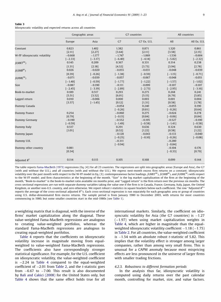
4.2. Results from pooling across developed countries

4.2.1. Standard Fama-MacBeth (1973) regressions

Table 3 extends our analysis to incorporate all23 developed countries. We report Fama-MacBeth coeffi-cients for Europe and Asia, the G7 (with and without theUnited States), and all countries (with and without theUnited States). To control for cross-country differences, orfixed effects, we include seven country dummies. The firstsix dummies correspond to non-U.S. countries in the G7(Canada, France, Germany, Italy, Japan, and the UnitedKingdom), and the last dummy corresponds to all otherdeveloped countries. Thus, this approach implicitly treats

the United States as a benchmark and measures cross-country differences relative to the U.S. market. In all theregressions, the country dummies are statistically insig-nificant, indicating that there are only modest country-specific effects after controlling for factor loadings andfirm characteristics.3

The first two columns of Table 3 show that high-idiosyncratic-volatility stocks in Europe and Asia also havelow expected returns. The coefficients on idiosyncraticvolatility are �0:67 and �1:18 for Europe and Asia,respectively, and are somewhat smaller in magnitudethan the U.S. coefficient of �2:01. These coefficients arehighly statistically significant. The third and fourthcolumns pool together all the G7 countries and separatelyconsider the effect of excluding the United States. Acrossall the G7 countries, the coefficient on W-FF idiosyncraticvolatility is �1:75, with a very negative robust t-statisticof �6:40. By construction, this coefficient is an average ofthe individual G7 country coefficients in Table 2. Clearly,the effect of low expected returns to stocks with highidiosyncratic volatility is very strong across the largestdeveloped markets. However, Table 3 makes clear that theU.S. effect dominates, since the coefficient on idiosyncraticvolatility falls to �1:07 when U.S. firms are excluded. Thiscoefficient has a t-statistic of �4:14.

The final two columns of Table 3 pool the data acrossall 23 developed countries. Pooled across all countries, thecoefficient on idiosyncratic volatility is �1:54 and highlysignificant. Because the interquartile range of W-FFidiosyncratic volatility is 50:5%� 20:3% ¼ 30:2% per an-num over all countries, there is a large economic decreaseof j � 1:54j � ð0:505� 0:203Þ ¼ 0:47% per month in mov-ing from the 25th to the 75th percentile of W-FFidiosyncratic volatility. When the United States is ex-cluded, the coefficient on idiosyncratic volatility falls inabsolute magnitude to �0:60 from �1:54, but this is stillsignificant with a robust t-statistic of �2:32. Thus, whilethe idiosyncratic volatility effect is concentrated in theUnited States, it is still strongly observed across the world.

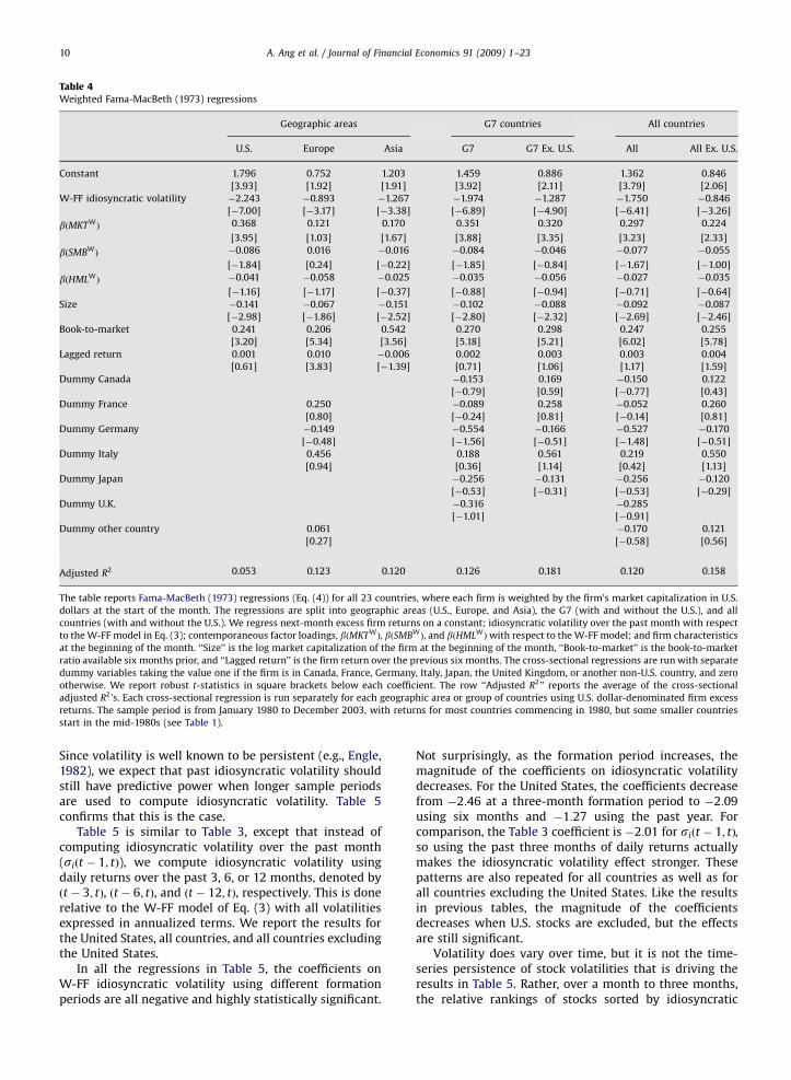
4.2.2. Robustness to value weighting

One potential concern about the use of cross-sectionalregressions is that each stock is treated equally in astandard Fama-MacBeth setting. Thus, even though weexclude very small stocks in each country, a standardFama-MacBeth regression places the same weight on avery large firm as on a small firm. Placing greater weighton small firms could generate noise, and although itmeasures the effect of a typical firm, it might not reflectthe effect of an average dollar. To allay these concerns,we report value-weighted Fama-MacBeth regressions inTable 4, where each return is weighted by the firm’smarket capitalization in U.S. dollars at the start of themonth. In the first stage, we perform GLS regressions with

ARTICLE IN PRESS

Table 3Idiosyncratic volatility and expected returns across all countries

Geographic areas G7 countries All countries

Europe Asia G7 G7 Ex. U.S. All All Ex. U.S.

Constant 0.823 1.402 1.382 0.871 1.320 0.861

[2.11] [2.27] [3.64] [2.11] [3.58] [2.15]

W-FF idiosyncratic volatility �0.668 �1.177 �1.747 �1.069 �1.536 �0.604

[�2.33] [�3.17] [�6.40] [�4.14] [�5.82] [�2.32]

bðMKTWÞ 0.145 0.209 0.367 0.331 0.314 0.238

[1.31] [2.18] [4.52] [3.73] [3.94] [2.78]

bðSMBWÞ 0.026 �0.020 �0.055 �0.031 �0.048 �0.039

[0.39] [�0.26] [�1.38] [�0.59] [�1.15] [�0.71]

bðHMLWÞ �0.071 �0.039 �0.057 �0.067 �0.048 �0.051

[�1.48] [�0.59] [�1.77] [�1.22] [�1.57] [�1.02]

Size �0.087 �0.190 �0.111 �0.099 �0.107 �0.107

[�2.45] [�3.19] [�2.89] [�2.73] [�2.95] [�3.16]

Book-to-market 0.189 0.517 0.293 0.275 0.268 0.241

[5.51] [3.52] [6.01] [5.15] [6.79] [5.85]

Lagged return 0.010 �0.006 0.000 0.003 0.001 0.004

[3.57] [�1.45] [0.12] [1.31] [0.58] [1.78]

Dummy Canada �0.054 0.240 �0.055 0.190

[�0.26] [0.81] [�0.26] [0.64]

Dummy France 0.254 �0.060 0.275 �0.024 0.278

[0.79] [�0.15] [0.84] [�0.06] [0.84]

Dummy Germany �0.190 �0.552 �0.195 �0.527 �0.190

[�0.59] [�1.49] [�0.58] [�1.41] [�0.58]

Dummy Italy 0.517 0.291 0.636 0.324 0.630

[1.01] [0.52] [1.22] [0.58] [1.22]

Dummy Japan �0.128 �0.043 �0.133 �0.040

[�0.25] [�0.10] [�0.26] [�0.08]

Dummy U.K. �0.311 �0.280

[�0.94] [�0.84]

Dummy other country 0.081 �0.104 0.176

[0.34] [�0.33] [0.79]

Adjusted R2 0.114 0.115 0.105 0.168 0.099 0.144

The table reports Fama-MacBeth (1973) regressions (Eq. (4)) for all 23 countries. The regressions are split into geographic areas (Europe and Asia), the G7

(with and without the U.S.), and all countries (with and without the U.S.). We regress next-month excess firm returns on a constant; idiosyncratic

volatility over the past month with respect to the W-FF model in Eq. (3); contemporaneous factor loadings, bðMKTWÞ, bðSMBW

Þ, and bðHMLWÞwith respect

to the W-FF model; and firm characteristics at the beginning of the month. ‘‘Size’’ is the log market capitalization of the firm at the beginning of the

month, ‘‘Book-to-market’’ is the book-to-market ratio available six months prior, and ‘‘Lagged return’’ is the firm return over the previous six months. The

cross-sectional regressions are run with separate dummy variables taking the value one if the firm is in Canada, France, Germany, Italy, Japan, the United

Kingdom, or another non-U.S. country, and zero otherwise. We report robust t-statistics in square brackets below each coefficient. The row ‘‘Adjusted R2’’

reports the average of the cross-sectional adjusted R2’s. Each cross-sectional regression is run separately for each geographic area or group of countries

using U.S. dollar-denominated firm excess returns. The sample period is from January 1980 to December 2003, with returns for most countries

commencing in 1980, but some smaller countries start in the mid-1980s (see Table 1).

A. Ang et al. / Journal of Financial Economics 91 (2009) 1–23 9

a weighting matrix that is diagonal, with the inverse of thefirms’ market capitalization along the diagonal. Thesevalue-weighted Fama-MacBeth regressions are analogousto creating value-weighted portfolios, whereas thestandard Fama-MacBeth regressions are analogous tocreating equal-weighted portfolios.

Table 4 reports that the coefficients on idiosyncraticvolatility increase in magnitude moving from equal-weighted to value-weighted Fama-MacBeth regressions.The coefficients also have correspondingly strongerstatistical significance. For example, for the U.S. coefficienton idiosyncratic volatility, the value-weighted coefficientis �2:24 in Table 4 compared to the equal-weightedcoefficient of �2:01 from Table 2, and the t-statistic goesfrom �6:67 to �7:00. This result is also documentedby Bali and Cakici (2008) for the United States only, butTable 4 shows that the same effect holds true for all

international markets. Similarly, the coefficient on idio-syncratic volatility for Asia (the G7 countries) is �1:27(�1:97) when using market capitalization weights inTable 4, which are higher in magnitude than the equal-weighted idiosyncratic volatility coefficient �1:18 (�1:75)in Table 2. For all countries, the value-weighted coefficientis �1:54 with an absolute robust t-statistic of 5.82. Thisimplies that the volatility effect is stronger among largercompanies, rather than among very small firms. This isunusual for a CAPM anomaly because most mispricingeffects are less pronounced in the universe of larger firmswith smaller trading frictions.

4.2.3. Robustness to different formation periods

In the analysis thus far, idiosyncratic volatility iscomputed using daily returns over the past calendarmonth, controlling for market, size, and value factors.

ARTICLE IN PRESS

Table 4Weighted Fama-MacBeth (1973) regressions

Geographic areas G7 countries All countries

U.S. Europe Asia G7 G7 Ex. U.S. All All Ex. U.S.

Constant 1.796 0.752 1.203 1.459 0.886 1.362 0.846

[3.93] [1.92] [1.91] [3.92] [2.11] [3.79] [2.06]

W-FF idiosyncratic volatility �2.243 �0.893 �1.267 �1.974 �1.287 �1.750 �0.846

[�7.00] [�3.17] [�3.38] [�6.89] [�4.90] [�6.41] [�3.26]

bðMKTWÞ 0.368 0.121 0.170 0.351 0.320 0.297 0.224

[3.95] [1.03] [1.67] [3.88] [3.35] [3.23] [2.33]

bðSMBWÞ �0.086 0.016 �0.016 �0.084 �0.046 �0.077 �0.055

[�1.84] [0.24] [�0.22] [�1.85] [�0.84] [�1.67] [�1.00]

bðHMLWÞ �0.041 �0.058 �0.025 �0.035 �0.056 �0.027 �0.035

[�1.16] [�1.17] [�0.37] [�0.88] [�0.94] [�0.71] [�0.64]

Size �0.141 �0.067 �0.151 �0.102 �0.088 �0.092 �0.087

[�2.98] [�1.86] [�2.52] [�2.80] [�2.32] [�2.69] [�2.46]

Book-to-market 0.241 0.206 0.542 0.270 0.298 0.247 0.255

[3.20] [5.34] [3.56] [5.18] [5.21] [6.02] [5.78]

Lagged return 0.001 0.010 �0.006 0.002 0.003 0.003 0.004

[0.61] [3.83] [�1.39] [0.71] [1.06] [1.17] [1.59]

Dummy Canada �0.153 0.169 �0.150 0.122

[�0.79] [0.59] [�0.77] [0.43]

Dummy France 0.250 �0.089 0.258 �0.052 0.260

[0.80] [�0.24] [0.81] [�0.14] [0.81]

Dummy Germany �0.149 �0.554 �0.166 �0.527 �0.170

[�0.48] [�1.56] [�0.51] [�1.48] [�0.51]

Dummy Italy 0.456 0.188 0.561 0.219 0.550

[0.94] [0.36] [1.14] [0.42] [1.13]

Dummy Japan �0.256 �0.131 �0.256 �0.120

[�0.53] [�0.31] [�0.53] [�0.29]

Dummy U.K. �0.316 �0.285

[�1.01] [�0.91]

Dummy other country 0.061 �0.170 0.121

[0.27] [�0.58] [0.56]

Adjusted R2 0.053 0.123 0.120 0.126 0.181 0.120 0.158

The table reports Fama-MacBeth (1973) regressions (Eq. (4)) for all 23 countries, where each firm is weighted by the firm’s market capitalization in U.S.

dollars at the start of the month. The regressions are split into geographic areas (U.S., Europe, and Asia), the G7 (with and without the U.S.), and all

countries (with and without the U.S.). We regress next-month excess firm returns on a constant; idiosyncratic volatility over the past month with respect

to the W-FF model in Eq. (3); contemporaneous factor loadings, bðMKTWÞ, bðSMBW

Þ, and bðHMLWÞwith respect to the W-FF model; and firm characteristics

at the beginning of the month. ‘‘Size’’ is the log market capitalization of the firm at the beginning of the month, ‘‘Book-to-market’’ is the book-to-market

ratio available six months prior, and ‘‘Lagged return’’ is the firm return over the previous six months. The cross-sectional regressions are run with separate

dummy variables taking the value one if the firm is in Canada, France, Germany, Italy, Japan, the United Kingdom, or another non-U.S. country, and zero

otherwise. We report robust t-statistics in square brackets below each coefficient. The row ‘‘Adjusted R2’’ reports the average of the cross-sectional

adjusted R2’s. Each cross-sectional regression is run separately for each geographic area or group of countries using U.S. dollar-denominated firm excess

returns. The sample period is from January 1980 to December 2003, with returns for most countries commencing in 1980, but some smaller countries

start in the mid-1980s (see Table 1).

A. Ang et al. / Journal of Financial Economics 91 (2009) 1–2310

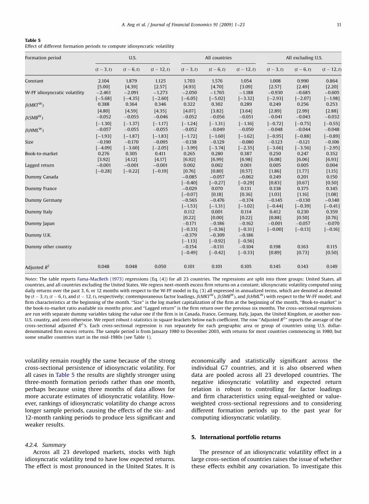
Since volatility is well known to be persistent (e.g., Engle,1982), we expect that past idiosyncratic volatility shouldstill have predictive power when longer sample periodsare used to compute idiosyncratic volatility. Table 5confirms that this is the case.

Table 5 is similar to Table 3, except that instead ofcomputing idiosyncratic volatility over the past month(siðt � 1; tÞ), we compute idiosyncratic volatility usingdaily returns over the past 3, 6, or 12 months, denoted byðt � 3; tÞ, ðt � 6; tÞ, and ðt � 12; tÞ, respectively. This is donerelative to the W-FF model of Eq. (3) with all volatilitiesexpressed in annualized terms. We report the results forthe United States, all countries, and all countries excludingthe United States.

In all the regressions in Table 5, the coefficients onW-FF idiosyncratic volatility using different formationperiods are all negative and highly statistically significant.

Not surprisingly, as the formation period increases, themagnitude of the coefficients on idiosyncratic volatilitydecreases. For the United States, the coefficients decreasefrom �2:46 at a three-month formation period to �2:09using six months and �1:27 using the past year. Forcomparison, the Table 3 coefficient is �2:01 for siðt � 1; tÞ,so using the past three months of daily returns actuallymakes the idiosyncratic volatility effect stronger. Thesepatterns are also repeated for all countries as well as forall countries excluding the United States. Like the resultsin previous tables, the magnitude of the coefficientsdecreases when U.S. stocks are excluded, but the effectsare still significant.

Volatility does vary over time, but it is not the time-series persistence of stock volatilities that is driving theresults in Table 5. Rather, over a month to three months,the relative rankings of stocks sorted by idiosyncratic

ARTICLE IN PRESS

Table 5Effect of different formation periods to compute idiosyncratic volatility

Formation period U.S. All countries All excluding U.S.

ðt � 3; tÞ ðt � 6; tÞ ðt � 12; tÞ ðt � 3; tÞ ðt � 6; tÞ ðt � 12; tÞ ðt � 3; tÞ ðt � 6; tÞ ðt � 12; tÞ

Constant 2.104 1.879 1.125 1.703 1.576 1.054 1.008 0.990 0.864

[5.00] [4.39] [2.57] [4.93] [4.70] [3.09] [2.57] [2.49] [2.20]

W-FF idiosyncratic volatility �2.461 �2.091 �1.273 �2.050 �1.765 �1.188 �0.930 �0.685 �0.605

[�5.68] [�4.35] [�2.60] [�6.05] [�5.02] [�3.32] [�2.93] [�2.07] [�1.98]

bðMKTWÞ 0.388 0.364 0.346 0.322 0.302 0.289 0.249 0.256 0.253

[4.80] [4.59] [4.35] [4.07] [3.82] [3.64] [2.89] [2.99] [2.88]

bðSMBWÞ �0.052 �0.055 �0.046 �0.052 �0.056 �0.051 �0.041 �0.043 �0.032

[�1.30] [�1.37] [�1.17] [�1.24] [�1.31] [�1.16] [�0.72] [�0.75] [�0.55]

bðHMLWÞ �0.057 �0.055 �0.055 �0.052 �0.049 �0.050 �0.048 �0.044 �0.048

[�1.93] [�1.87] [�1.83] [�1.72] [�1.60] [�1.62] [�0.95] [�0.88] [�0.89]

Size �0.190 �0.170 �0.095 �0.138 �0.129 �0.080 �0.123 �0.121 �0.106

[�4.09] [�3.60] [�2.05] [�3.99] [�3.74] [�2.35] [�3.66] [�3.56] [�2.95]

Book-to-market 0.276 0.305 0.411 0.265 0.280 0.387 0.250 0.247 0.352

[3.92] [4.12] [4.17] [6.92] [6.99] [6.98] [6.08] [6.06] [6.93]

Lagged return �0.001 �0.001 �0.001 0.002 0.002 0.001 0.005 0.005 0.004

[�0.28] [�0.22] [�0.19] [0.76] [0.80] [0.57] [1.86] [1.77] [1.15]

Dummy Canada �0.085 �0.057 �0.062 0.249 0.201 0.150

[�0.40] [�0.27] [�0.29] [0.83] [0.67] [0.50]

Dummy France �0.029 0.070 0.131 0.338 0.375 0.345

[�0.07] [0.18] [0.36] [1.03] [1.16] [1.08]

Dummy Germany �0.565 �0.476 �0.374 �0.145 �0.130 �0.140

[�1.53] [�1.31] [�1.02] [�0.44] [�0.39] [�0.41]

Dummy Italy 0.112 0.001 0.114 0.412 0.230 0.359

[0.22] [0.00] [0.22] [0.88] [0.50] [0.76]

Dummy Japan �0.171 �0.186 �0.162 �0.001 �0.057 �0.070

[�0.33] [�0.36] [�0.31] [�0.00] [�0.13] [�0.16]

Dummy U.K. �0.379 �0.309 �0.186

[�1.13] [�0.92] [�0.56]

Dummy other country �0.154 �0.131 �0.104 0.198 0.163 0.115

[�0.49] [�0.42] [�0.33] [0.89] [0.73] [0.50]

Adjusted R2 0.048 0.048 0.050 0.101 0.101 0.105 0.145 0.143 0.149

Notes: The table reports Fama-MacBeth (1973) regressions (Eq. (4)) for all 23 countries. The regressions are split into three groups: United States, all

countries, and all countries excluding the United States. We regress next-month excess firm returns on a constant; idiosyncratic volatility computed using

daily returns over the past 3, 6, or 12 months with respect to the W-FF model in Eq. (3) all expressed in annualized terms, which are denoted as denoted

by ðt � 3; tÞ, ðt � 6; tÞ, and ðt � 12; tÞ, respectively; contemporaneous factor loadings, bðMKTWÞ, bðSMBW

Þ, and bðHMLWÞwith respect to the W-FF model; and

firm characteristics at the beginning of the month. ‘‘Size’’ is the log market capitalization of the firm at the beginning of the month, ‘‘Book-to-market’’ is

the book-to-market ratio available six months prior, and ‘‘Lagged return’’ is the firm return over the previous six months. The cross-sectional regressions

are run with separate dummy variables taking the value one if the firm is in Canada, France, Germany, Italy, Japan, the United Kingdom, or another non-

U.S. country, and zero otherwise. We report robust t-statistics in square brackets below each coefficient. The row ‘‘Adjusted R2’’ reports the average of the

cross-sectional adjusted R2’s. Each cross-sectional regression is run separately for each geographic area or group of countries using U.S. dollar-

denominated firm excess returns. The sample period is from January 1980 to December 2003, with returns for most countries commencing in 1980, but

some smaller countries start in the mid-1980s (see Table 1).

A. Ang et al. / Journal of Financial Economics 91 (2009) 1–23 11

volatility remain roughly the same because of the strongcross-sectional persistence of idiosyncratic volatility. Forall cases in Table 5 the results are slightly stronger usingthree-month formation periods rather than one month,perhaps because using three months of data allows formore accurate estimates of idiosyncratic volatility. How-ever, rankings of idiosyncratic volatility do change acrosslonger sample periods, causing the effects of the six- and12-month ranking periods to produce less significant andweaker results.

4.2.4. Summary

Across all 23 developed markets, stocks with highidiosyncratic volatility tend to have low expected returns.The effect is most pronounced in the United States. It is

economically and statistically significant across theindividual G7 countries, and it is also observed whendata are pooled across all 23 developed countries. Thenegative idiosyncratic volatility and expected returnrelation is robust to controlling for factor loadingsand firm characteristics using equal-weighted or value-weighted cross-sectional regressions and to consideringdifferent formation periods up to the past year forcomputing idiosyncratic volatility.

5. International portfolio returns

The presence of an idiosyncratic volatility effect in alarge cross-section of countries raises the issue of whetherthese effects exhibit any covariation. To investigate this

ARTICLE IN PRESS

A. Ang et al. / Journal of Financial Economics 91 (2009) 1–2312

we create idiosyncratic volatility portfolios across regionsand across all 23 countries.

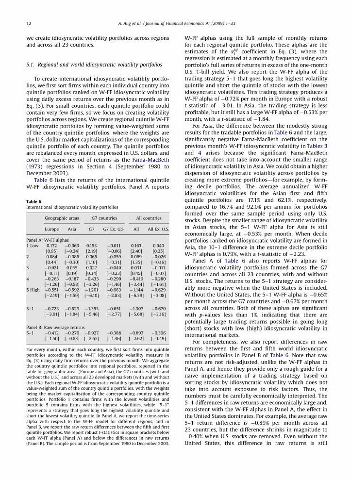
5.1. Regional and world idiosyncratic volatility portfolios

To create international idiosyncratic volatility portfo-lios, we first sort firms within each individual country intoquintile portfolios ranked on W-FF idiosyncratic volatilityusing daily excess returns over the previous month as inEq. (3). For small countries, each quintile portfolio couldcontain very few firms, so we focus on creating volatilityportfolios across regions. We create regional quintile W-FFidiosyncratic portfolios by forming value-weighted sumsof the country quintile portfolios, where the weights arethe U.S. dollar market capitalizations of the correspondingquintile portfolio of each country. The quintile portfoliosare rebalanced every month, expressed in U.S. dollars, andcover the same period of returns as the Fama-MacBeth(1973) regressions in Section 4 (September 1980 toDecember 2003).

Table 6 lists the returns of the international quintileW-FF idiosyncratic volatility portfolios. Panel A reports

Table 6International idiosyncratic volatility portfolios

Geographic areas G7 countries All countries

Europe Asia G7 G7 Ex. U.S. All All Ex. U.S.

Panel A: W-FF alphas

1 Low 0.172 �0.063 0.153 �0.011 0.163 0.040

[0.95] [�0.24] [2.19] [�0.06] [2.40] [0.25]

2 0.084 �0.086 0.065 �0.059 0.069 �0.026

[0.44] [�0.30] [1.16] [�0.31] [1.35] [�0.16]

3 �0.021 0.055 0.027 �0.040 0.031 �0.011

[�0.11] [0.19] [0.34] [�0.23] [0.45] [�0.07]

4 �0.263 �0.187 �0.433 �0.290 �0.416 �0.280

[�1.26] [�0.58] [�3.26] [�1.46] [�3.44] [�1.61]

5 High �0.551 �0.592 �1.201 �0.663 �1.144 �0.629

[�2.19] [�1.59] [�6.10] [�2.83] [�6.39] [�3.08]

5–1 �0.723 �0.529 �1.353 �0.651 �1.307 �0.670

[�3.01] [�1.84] [�5.46] [�2.77] [�5.68] [�3.16]

Panel B: Raw average returns

5–1 �0.412 �0.270 �0.927 �0.388 �0.893 �0.396

[�1.50] [�0.83] [�2.55] [�1.36] [�2.62] [�1.49]

For every month, within each country, we first sort firms into quintile

portfolios according to the W-FF idiosyncratic volatility measure in

Eq. (3) using daily firm returns over the previous month. We aggregate

the country quintile portfolios into regional portfolios, reported in the

table for geographic areas (Europe and Asia), the G7 countries (with and

without the U.S.), and across all 23 developed markets (with and without

the U.S.). Each regional W-FF idiosyncratic volatility quintile portfolio is a

value-weighted sum of the country quintile portfolios, with the weights

being the market capitalization of the corresponding country quintile

portfolios. Portfolio 1 contains firms with the lowest volatilities and

portfolio 5 contains firms with the highest volatilities, while ‘‘5–1’’

represents a strategy that goes long the highest volatility quintile and

short the lowest volatility quintile. In Panel A, we report the time-series

alpha with respect to the W-FF model for different regions, and in

Panel B, we report the raw return differences between the fifth and first

quintile portfolios. We report robust t-statistics in square brackets below

each W-FF alpha (Panel A) and below the differences in raw returns

(Panel B). The sample period is from September 1980 to December 2003.

W-FF alphas using the full sample of monthly returnsfor each regional quintile portfolio. These alphas are theestimates of the aW

i coefficient in Eq. (3), where theregression is estimated at a monthly frequency using eachportfolio’s full series of returns in excess of the one-monthU.S. T-bill yield. We also report the W-FF alpha of thetrading strategy 5–1 that goes long the highest volatilityquintile and short the quintile of stocks with the lowestidiosyncratic volatilities. This trading strategy produces aW-FF alpha of �0:72% per month in Europe with a robustt-statistic of �3:01. In Asia, the trading strategy is lessprofitable, but it still has a large W-FF alpha of �0:53% permonth, with a t-statistic of �1:84.

For Asia, the difference between the modestly strongresults for the tradable portfolios in Table 6 and the large,significantly negative Fama-MacBeth coefficient on theprevious month’s W-FF idiosyncratic volatility in Tables 3and 4 arises because the significant Fama-MacBethcoefficient does not take into account the smaller rangeof idiosyncratic volatility in Asia. We could obtain a higherdispersion of idiosyncratic volatility across portfolios bycreating more extreme portfolios—for example, by form-ing decile portfolios. The average annualized W-FFidiosyncratic volatilities for the Asian first and fifthquintile portfolios are 17.1% and 62.1%, respectively,compared to 16.7% and 92.0% per annum for portfoliosformed over the same sample period using only U.S.stocks. Despite the smaller range of idiosyncratic volatilityin Asian stocks, the 5–1 W-FF alpha for Asia is stilleconomically large, at �0:53% per month. When decileportfolios ranked on idiosyncratic volatility are formed inAsia, the 10–1 difference in the extreme decile portfolioW-FF alphas is 0.79%, with a t-statistic of �2:23.

Panel A of Table 6 also reports W-FF alphas foridiosyncratic volatility portfolios formed across the G7countries and across all 23 countries, with and withoutU.S. stocks. The returns to the 5–1 strategy are consider-ably more negative when the United States is included.Without the United States, the 5–1 W-FF alpha is �0:65%per month across the G7 countries and �0:67% per monthacross all countries. Both of these alphas are significantwith p-values less than 1%, indicating that there arepotentially large trading returns possible in going long(short) stocks with low (high) idiosyncratic volatility ininternational markets.

For completeness, we also report differences in rawreturns between the first and fifth world idiosyncraticvolatility portfolios in Panel B of Table 6. Note that rawreturns are not risk-adjusted, unlike the W-FF alphas inPanel A, and hence they provide only a rough guide for anaı̈ve implementation of a trading strategy based onsorting stocks by idiosyncratic volatility which does nottake into account exposure to risk factors. Thus, thenumbers must be carefully economically interpreted. The5–1 differences in raw returns are economically large and,consistent with the W-FF alphas in Panel A, the effect inthe United States dominates. For example, the average raw5–1 return difference is �0:89% per month across all23 countries, but the difference shrinks in magnitude to�0:40% when U.S. stocks are removed. Even without theUnited States, this difference in raw returns is still

ARTICLE IN PRESS

A. Ang et al. / Journal of Financial Economics 91 (2009) 1–23 13

economically large, but only when the United States isincluded are the differences in raw returns statisticallysignificant.

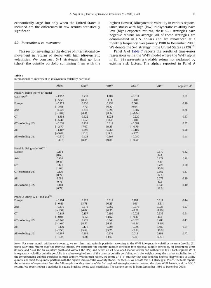
5.2. International co-movement

This section investigates the degree of international co-movement in returns of stocks with high idiosyncraticvolatilities. We construct 5–1 strategies that go long(short) the quintile portfolio containing firms with the

Table 7International co-movement in idiosyncratic volatility portfolios

Alpha MKTW SM

Panel A: Using the W-FF model

U.S. (VOLUS) �1.952 0.733 1.

[�5.59] [8.56] [1

Europe �0.723 0.456 0.

[�3.01] [7.72] [6

Asia �0.529 0.339 0.

[�1.84] [4.82] [8

G7 �1.353 0.622 1.

[�5.46] [10.2] [1

G7 excluding U.S. �0.651 0.432 0.

[�2.77] [7.49] [9

All �1.307 0.596 0.

[�5.69] [10.6] [1

All excluding U.S. �0.670 0.428 0.

[�3.16] [8.24] [9

Panel B: Using only VOLUS

Europe 0.134

[0.63]

Asia 0.130

[0.43]

G7 0.121

[1.04]

G7 excluding U.S. 0.176

[0.77]

All 0.081

[0.71]

All excluding U.S. 0.148

[0.71]

Panel C: Using W-FF and VOLUS

Europe �0.104 0.223 0.

[�0.46] [3.78] [0

Asia �0.475 0.319 0.

[�1.57] [4.02] [6

G7 �0.115 0.157 0.

[�0.98] [5.12] [4

G7 excluding U.S. �0.245 0.279 0.

[�1.04] [4.52] [4

All �0.176 0.171 0.

[�1.53] [5.69] [5

All excluding U.S. �0.283 0.283 0.

[�1.34] [5.11] [4

Notes: For every month, within each country, we sort firms into quintile portfo

using daily firm returns over the previous month. We aggregate the country

(Europe and Asia), the G7 countries (with and without the U.S.), and across all

idiosyncratic volatility quintile portfolio is a value-weighted sum of the countr

the corresponding quintile portfolios in each country. Within each region, we c

quintile and short the quintile portfolio with the highest idiosyncratic volatility s

the estimates of regressions from the full sample monthly returns of the 5–1 r

returns. We report robust t-statistics in square brackets below each coefficient

highest (lowest) idiosyncratic volatility in various regions.Since stocks with high (low) idiosyncratic volatility havelow (high) expected returns, these 5–1 strategies earnnegative returns on average. All of these strategies aredenominated in U.S. dollars and are rebalanced at amonthly frequency over January 1980 to December 2003.We denote the 5–1 strategy in the United States as VOLUS.

Panel A of Table 7 reports the results of time-seriesregressions using the W-FF model where the W-FF alphain Eq. (3) represents a tradable return not explained byexisting risk factors. The alphas reported in Panel A

BW HMLW VOLUS Adjusted R2

307 �0.311 0.51

3.1] [�1.88]

433 0.004 0.29

.32] [0.04]

699 �0.087 0.28

.54] [�0.64]

028 �0.220 0.57

4.6] [�1.88]

618 �0.087 0.37

.23] [�0.79]

966 �0.189 0.58

4.8] [�1.75]

597 �0.050 0.41

.89] [�0.50]

0.370 0.42

[14.1]

0.271 0.16

[7.29]

0.723 0.90

[50.6]

0.362 0.37

[12.8]

0.673 0.89

[47.6]

0.348 0.40

[13.6]

018 0.103 0.317 0.44

.23] [1.01] [8.61]

662 �0.078 0.028 0.27

.35] [�0.57] [0.56]

199 �0.023 0.635 0.91

.92] [�0.43] [33.1]

346 �0.023 0.208 0.43

.25] [�0.21] [5.40]

208 �0.009 0.580 0.91

.25] [�0.18] [30.9]

338 0.012 0.198 0.47

.63] [0.13] [5.73]

lios according to the W-FF idiosyncratic volatility measure (see Eq. (3))

quintile portfolios into regional quintile portfolios, for geographic areas

23 developed markets (with and without the U.S.). Each regional W-FF

y quintile portfolios, with the weights being the market capitalization of

reate a ‘‘5–1’’ strategy that goes long the highest idiosyncratic volatility

tocks. For the U.S., we denote this 5–1 strategy as VOLUS. The table reports

egional strategies onto a constant, the three W-FF factors, and the VOLUS

. The sample period is from September 1980 to December 2003.

ARTICLE IN PRESS

A. Ang et al. / Journal of Financial Economics 91 (2009) 1–2314

correspond to the 5–1 alphas reported in Table 6. Theseregressions serve as a base case for investigating how theinternational 5–1 idiosyncratic volatility strategies arerelated to the 5–1 strategy in the United States, VOLUS, inPanels B and C. In our discussion, we focus on thegeographic areas excluding the United States, since, byconstruction, we can always partly explain regionalreturns that include the United States with U.S. returns.Nevertheless, we include all the regions in Table 7 forcompleteness.

Panel B shows that there are large and significant co-movements between the idiosyncratic volatility portfolioreturns in international markets and in the United States.If the 5–1 idiosyncratic volatility portfolio returns areregressed only on a constant and VOLUS, the alphas are allstatistically insignificant. The VOLUS loadings range from0.27 for Asia to 0.36 for the G7 countries excluding the U.S.market. All of these VOLUS loadings are highly statisticallysignificant, with the lowest absolute t-statistic occurringfor Asia at 7.29.

Controlling for the W-FF factors in Panel C also doesnot generally remove the explanatory power of the VOLUS

returns for the international idiosyncratic volatilitytrading strategies. For Europe, the loading of 0.32 onVOLUS is similar to the 0.37 loading without W-FF factors.The coefficient on VOLUS for the G7 excluding the UnitedStates falls slightly from 0.72 to 0.63, while the corre-sponding loading for all countries excluding the UnitedStates decreases from 0.67 to 0.58 when the W-FF factorsare added. These coefficients are still highly significantwith t-statistics above 5.4. Only in the case of Asia is theloading on VOLUS small, at 0.03, after adding the W-FFfactors.

In summary, there are remarkably similar returnsacross the international idiosyncratic volatility portfolios.Trading strategies that go long stocks with high idiosyn-cratic volatility and go short low-idiosyncratic-volatilitystocks in foreign markets have large exposures to thesame idiosyncratic volatility trading strategy using onlyU.S. stocks. After controlling for the exposure to the UnitedStates, there are no excess returns. Without controlling forU.S. exposure, however, the low returns to high-idiosyn-cratic-volatility stocks cannot be explained by standardrisk factors. This high degree of covariation suggests thatwhat is driving the very low returns to high-idiosyncratic-volatility stocks around the world cannot be easilydiversified away and is dominated by U.S. effects.

4 AHXZ also include market volatility and liquidity risk factors in

their analysis of U.S. data, and neither factor explains the returns to

portfolios sorted on past idiosyncratic volatility. Because these factors

are difficult to measure with international data, we did not include them

in this paper. Adrian and Rosenberg (2007) argue that the U.S. market

volatility risk factor can be split into short-run and long-run compo-

nents. Neither of these risk factors explains the anomalous low returns of

stocks with high idiosyncratic volatility. These results are available upon

request.

6. A more detailed look at the United States

Sections 4 and 5 show that around the world, stockswith high idiosyncratic volatility have low returns. Theeffect is strongest in the United States, and we observesignificant covariation between the returns of high-idiosyncratic-volatility stocks in non-U.S. countries withthe returns of high-idiosyncratic-volatility stocks in theUnited States. This warrants a detailed look at the effect inU.S. data, where a relatively large number of firms allowsfor greater power in investigating the cross-sectionaldeterminants of the effect. The U.S. market also has more

detailed data on trading costs and other market frictionsthan other countries to facilitate the analysis.

AHXZ show that the U.S. idiosyncratic volatility effectis robust to controlling for standard risk and firmcharacteristics such as size, value, liquidity, and co-skewness. They find that exposure to aggregate marketvolatility risk measured by VIX cannot explain the effect.4

Simple microstructure measures, volume, turnover, andbid–ask spreads also cannot explain the phenomenon.Dispersion in analysts’ forecasts is also not an explanation.AHXZ report that the idiosyncratic volatility effect isrobust to controlling for momentum strategies using one-,six-, and 12-month past returns, and they show that theidiosyncratic volatility effect persists for holding periodsof up to at least one year.

In Section 6.1 we outline other potential economicexplanations based on the costs of trading and informa-tion dissemination. We go beyond AHXZ in using bettermeasures of transaction costs; in particular, we use arecently developed measure for assessing the amount ofprivate information in trades. We also examine economicstories regarding how different types of investor clientelesmight analyze and process information. Stocks withdifferent idiosyncratic volatility could have differentexposures to these risk factors. We also consider theeffects of investor preferences for skewness. Examiningthese economic sources of risk is important because pastresearch has established them to be important determi-nants of other CAPM anomalies.

Section 6.2 shows that the low returns to high-idiosyncratic-volatility stocks survive after controllingfor these explanations. In Section 6.3, we constructinvestable portfolios based on idiosyncratic volatilitywhile controlling for other relevant variables. Section 6.4focuses on how lagged idiosyncratic volatility is related toexpected future volatility and examines whether anoption hypothesis proposed by Johnson (2004) canexplain our findings.

6.1. Potential economic explanations

6.1.1. Private information

Easley and O’Hara (2004) argue that expected stockreturns differ because of differences in the amount ofprivate information embedded in the trades of thosestocks. Specifically, stocks with more private informationcommand higher expected returns. To measure the degreeof private information contained in the trading activity ofeach stock, Easley, Hvidkjaer, and O’Hara (2002) constructa measure of private information, denoted PIN. They showthat stocks with high PINs have significantly higher

ARTICLE IN PRESS

5 AHXZ rule out that exposure to coskewness (see Harvey and

Siddique, 2000) can explain the low returns of stocks with high

idiosyncratic volatility.

A. Ang et al. / Journal of Financial Economics 91 (2009) 1–23 15

expected returns than stocks with low PINs. It is possiblethat stocks with low (high) idiosyncratic volatility arestocks whose trades contain very high (low) amounts ofprivate information. This situation would explain therelatively high returns on low-volatility stocks and lowreturns on high-volatility stocks. One drawback of the PINmeasure is that it is constructed using intraday trades,which restricts the sample to post-1984.

6.1.2. Transaction costs

Lesmond, Ogden, and Trzcinka (1999) construct ameasure of transaction costs using the proportion of dailyreturns equal to zero each month. They demonstratethat this measure is highly correlated with spread andcommission estimates of transaction costs. A majoradvantage of their measure is that it only requires dailyreturns, allowing the use of long time series. We examineif the volatility effect is concentrated in stocks with thehighest transaction costs where arbitrage is difficult.

6.1.3. Analyst coverage

Stocks with few analysts might incorporate newinformation into prices more slowly. Hou and Moskowitz(2005) hypothesize that if investors value fast informationdissemination, stocks covered by fewer analysts will havehigher returns than stocks tracked by many analysts. Ifstocks with low volatility have low amounts of analystcoverage, these stocks would require higher returns tocompensate for the slower dissemination of news.Following Diether, Malloy, and Scherbina (2002), wedefine analyst coverage as the number of analystsproviding current fiscal year annual earnings estimateseach month in the I/B/E/S database, which is availablefrom July 1976 onwards. Controlling for the amount ofanalyst coverage skews our sample toward larger firms,which tend to be covered by more analysts than are smallfirms.

6.1.4. Institutional ownership

Stocks with lower amounts of institutional ownershiptend to be stocks with more uninformed traders (see, e.g.,Kumar, 2007). Naturally, stocks with low institutionalholdings tend to be stocks that are followed less closely byanalysts. These stocks also tend to be smaller and moreilliquid, and their prices could respond more slowly tonews announcements. Stocks with low idiosyncraticvolatility could be stocks with low levels of institutionalownership, causing these stocks to have high averagereturns. Institutional ownership data come from Standard& Poor’s and starts in July 1981.

6.1.5. Delay

Hou and Moskowitz (2005) develop a new measurethat captures how fast a stock’s price responds toinformation. To construct this measure, they regress eachstock’s weekly returns on contemporaneous and laggedmarket returns. If a stock responds immediately to marketnews, coefficients on the lagged market returns will equalzero and there will be no improvement in the R2 fromadding the lagged market return to the regression. TheHou-Moskowitz delay measure uses the ratio of the R2

from a regression with only a contemporaneous marketreturn to the R2 from a regression with both contempora-neous and lagged market returns. They find that the mostseverely delayed firms command large return premiums.These stocks could be low-idiosyncratic-volatility stocksthat have high returns because their prices respond slowlyto new information. We use the Hou and Moskowitz delaymeasure starting from 1965.

6.1.6. Skewness

Barberis and Huang (2005) develop a behavioralsetting in which the individual skewness of stock returnsmight be priced.5 Under the cumulative prospect theorypreferences of Tversky and Kahneman (1992), investorstransform objective probabilities using a weighting func-tion that overweights the tails of the probability distribu-tion. This causes positively skewed securities to becomeoverpriced and to earn negative average excess returns. Ifhigh-idiosyncratic-volatility stocks are stocks with posi-tive skewness, the Barberis and Huang argument wouldexplain why stocks with high idiosyncratic volatility havelow returns.

6.2. Cross-sectional regression results

In order to control for these potential economicexplanations of the idiosyncratic volatility phenomenon,we include the characteristic controls described abovewith other risk controls in Fama-MacBeth (1973) regres-sions along with the L-FF idiosyncratic volatility measuredover the past month. Table 8 reports time-series averagecoefficients from seven cross-sectional regression specifi-cations for U.S. data. All of the specifications control forcontemporaneous L-FF factor loadings and for past size,book-to-market, and momentum characteristics. Thespecifications use different numbers of stocks because ofdata availability issues. In regressions I–VI, we separatelyinclude the Easley, Hvidkjaer, and O’Hara’s (2002) PINmeasure, the percentage of zero returns, the number ofanalysts, the proportion of institutional ownership, theHou and Moskowitz (2005) delay measure, and theindividual skewness of the return. Regressions I, III, andIV control for these variables as constructed by otherauthors, which approximately halves our full sampleperiod and takes many fewer stocks. In regression VII,we include all of the various control variables, except PINbecause of its shorter sample. All the cross-sectionalregressions are rerun every month. Because of the datarequirements of book values and past six-month returns,the dependent variable returns of these regressions beginseven months after the beginning of the sample periodlisted in Table 8.

Panel A shows that in all of the regression specifica-tions, the Fama-MacBeth coefficient on L-FF idiosyncraticvolatility is negative and strongly significant. In contrast,in regressions I–V, the coefficients on the control variables

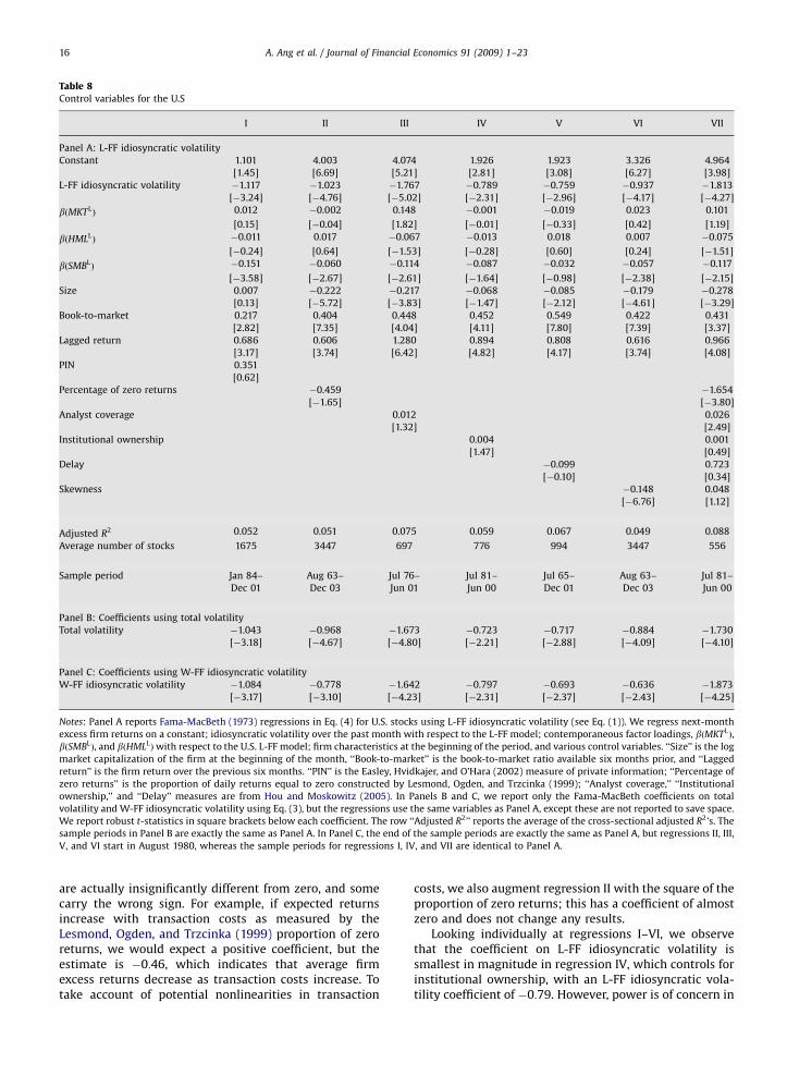
ARTICLE IN PRESS

Table 8Control variables for the U.S

I II III IV V VI VII

Panel A: L-FF idiosyncratic volatility

Constant 1.101 4.003 4.074 1.926 1.923 3.326 4.964

[1.45] [6.69] [5.21] [2.81] [3.08] [6.27] [3.98]

L-FF idiosyncratic volatility �1.117 �1.023 �1.767 �0.789 �0.759 �0.937 �1.813

[�3.24] [�4.76] [�5.02] [�2.31] [�2.96] [�4.17] [�4.27]

bðMKTLÞ 0.012 �0.002 0.148 �0.001 �0.019 0.023 0.101

[0.15] [�0.04] [1.82] [�0.01] [�0.33] [0.42] [1.19]

bðHMLLÞ �0.011 0.017 �0.067 �0.013 0.018 0.007 �0.075

[�0.24] [0.64] [�1.53] [�0.28] [0.60] [0.24] [�1.51]

bðSMBLÞ �0.151 �0.060 �0.114 �0.087 �0.032 �0.057 �0.117

[�3.58] [�2.67] [�2.61] [�1.64] [�0.98] [�2.38] [�2.15]

Size 0.007 �0.222 �0.217 �0.068 �0.085 �0.179 �0.278

[0.13] [�5.72] [�3.83] [�1.47] [�2.12] [�4.61] [�3.29]

Book-to-market 0.217 0.404 0.448 0.452 0.549 0.422 0.431

[2.82] [7.35] [4.04] [4.11] [7.80] [7.39] [3.37]

Lagged return 0.686 0.606 1.280 0.894 0.808 0.616 0.966

[3.17] [3.74] [6.42] [4.82] [4.17] [3.74] [4.08]

PIN 0.351

[0.62]

Percentage of zero returns �0.459 �1.654

[�1.65] [�3.80]

Analyst coverage 0.012 0.026

[1.32] [2.49]

Institutional ownership 0.004 0.001

[1.47] [0.49]

Delay �0.099 0.723

[�0.10] [0.34]

Skewness �0.148 0.048

[�6.76] [1.12]

Adjusted R2 0.052 0.051 0.075 0.059 0.067 0.049 0.088

Average number of stocks 1675 3447 697 776 994 3447 556

Sample period Jan 84– Aug 63– Jul 76– Jul 81– Jul 65– Aug 63– Jul 81–

Dec 01 Dec 03 Jun 01 Jun 00 Dec 01 Dec 03 Jun 00

Panel B: Coefficients using total volatility

Total volatility �1.043 �0.968 �1.673 �0.723 �0.717 �0.884 �1.730

[�3.18] [�4.67] [�4.80] [�2.21] [�2.88] [�4.09] [�4.10]

Panel C: Coefficients using W-FF idiosyncratic volatility

W-FF idiosyncratic volatility �1.084 �0.778 �1.642 �0.797 �0.693 �0.636 �1.873

[�3.17] [�3.10] [�4.23] [�2.31] [�2.37] [�2.43] [�4.25]

Notes: Panel A reports Fama-MacBeth (1973) regressions in Eq. (4) for U.S. stocks using L-FF idiosyncratic volatility (see Eq. (1)). We regress next-month

excess firm returns on a constant; idiosyncratic volatility over the past month with respect to the L-FF model; contemporaneous factor loadings, bðMKTLÞ,

bðSMBLÞ, and bðHMLL

Þwith respect to the U.S. L-FF model; firm characteristics at the beginning of the period, and various control variables. ‘‘Size’’ is the log

market capitalization of the firm at the beginning of the month, ‘‘Book-to-market’’ is the book-to-market ratio available six months prior, and ‘‘Lagged

return’’ is the firm return over the previous six months. ‘‘PIN’’ is the Easley, Hvidkajer, and O’Hara (2002) measure of private information; ‘‘Percentage of

zero returns’’ is the proportion of daily returns equal to zero constructed by Lesmond, Ogden, and Trzcinka (1999); ‘‘Analyst coverage,’’ ‘‘Institutional

ownership,’’ and ‘‘Delay’’ measures are from Hou and Moskowitz (2005). In Panels B and C, we report only the Fama-MacBeth coefficients on total

volatility and W-FF idiosyncratic volatility using Eq. (3), but the regressions use the same variables as Panel A, except these are not reported to save space.

We report robust t-statistics in square brackets below each coefficient. The row ‘‘Adjusted R2’’ reports the average of the cross-sectional adjusted R2’s. The

sample periods in Panel B are exactly the same as Panel A. In Panel C, the end of the sample periods are exactly the same as Panel A, but regressions II, III,

V, and VI start in August 1980, whereas the sample periods for regressions I, IV, and VII are identical to Panel A.

A. Ang et al. / Journal of Financial Economics 91 (2009) 1–2316

are actually insignificantly different from zero, and somecarry the wrong sign. For example, if expected returnsincrease with transaction costs as measured by theLesmond, Ogden, and Trzcinka (1999) proportion of zeroreturns, we would expect a positive coefficient, but theestimate is �0:46, which indicates that average firmexcess returns decrease as transaction costs increase. Totake account of potential nonlinearities in transaction

costs, we also augment regression II with the square of theproportion of zero returns; this has a coefficient of almostzero and does not change any results.

Looking individually at regressions I–VI, we observethat the coefficient on L-FF idiosyncratic volatility issmallest in magnitude in regression IV, which controls forinstitutional ownership, with an L-FF idiosyncratic vola-tility coefficient of �0:79. However, power is of concern in

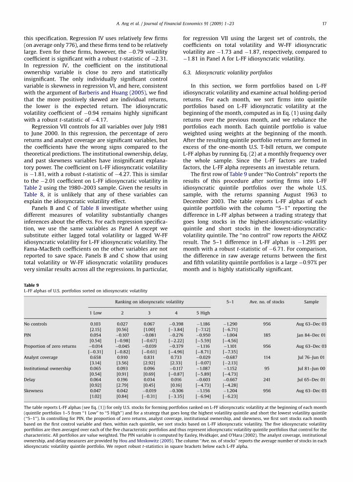
ARTICLE IN PRESS

A. Ang et al. / Journal of Financial Economics 91 (2009) 1–23 17

this specification. Regression IV uses relatively few firms(on average only 776), and these firms tend to be relativelylarge. Even for these firms, however, the �0:79 volatilitycoefficient is significant with a robust t-statistic of �2:31.In regression IV, the coefficient on the institutionalownership variable is close to zero and statisticallyinsignificant. The only individually significant controlvariable is skewness in regression VI, and here, consistentwith the argument of Barberis and Huang (2005), we findthat the more positively skewed are individual returns,the lower is the expected return. The idiosyncraticvolatility coefficient of �0:94 remains highly significantwith a robust t-statistic of �4:17.

Regression VII controls for all variables over July 1981to June 2000. In this regression, the percentage of zeroreturns and analyst coverage are significant variables, butthe coefficients have the wrong signs compared to thetheoretical predictions. The institutional ownership, delay,and past skewness variables have insignificant explana-tory power. The coefficient on L-FF idiosyncratic volatilityis �1:81, with a robust t-statistic of �4:27. This is similarto the �2:01 coefficient on L-FF idiosyncratic volatility inTable 2 using the 1980–2003 sample. Given the results inTable 8, it is unlikely that any of these variables canexplain the idiosyncratic volatility effect.

Panels B and C of Table 8 investigate whether usingdifferent measures of volatility substantially changesinferences about the effects. For each regression specifica-tion, we use the same variables as Panel A except wesubstitute either lagged total volatility or lagged W-FFidiosyncratic volatility for L-FF idiosyncratic volatility. TheFama-MacBeth coefficients on the other variables are notreported to save space. Panels B and C show that usingtotal volatility or W-FF idiosyncratic volatility producesvery similar results across all the regressions. In particular,

Table 9L-FF alphas of U.S. portfolios sorted on idiosyncratic volatility

Ranking on idiosyncratic volatilit

1 Low 2 3 4

No controls 0.103 0.027 0.067 �0.398

[2.15] [0.56] [1.00] [�3.84

PIN 0.054 �0.107 �0.081 �0.276

[0.54] [�0.98] [�0.67] [�2.22

Proportion of zero returns �0.014 �0.045 �0.039 �0.379

[�0.31] [�0.82] [�0.61] [�4.96

Analyst coverage 0.658 0.910 0.831 0.733

[3.14] [3.56] [2.92] [2.33]

Institutional ownership 0.065 0.093 0.096 �0.117

[0.54] [0.91] [0.69] [�0.87

Delay 0.064 0.196 0.034 0.016

[0.92] [2.79] [0.45] [0.16]

Skewness 0.047 0.042 �0.019 �0.306

[1.02] [0.84] [�0.31] [�3.35

The table reports L-FF alphas (see Eq. (1)) for only U.S. stocks for forming portfol

(quintile portfolios 1–5 from ‘‘1 Low’’ to ‘‘5 High’’) and for a strategy that goes l

(‘‘5–1’’). In controlling for PIN, the proportion of zero returns, analyst coverage

based on the first control variable and then, within each quintile, we sort stoc

portfolios are then averaged over each of the five characteristic portfolios and th

characteristic. All portfolios are value weighted. The PIN variable is computed by

ownership, and delay measures are provided by Hou and Moskowitz (2005). The

idiosyncratic volatility quintile portfolio. We report robust t-statistics in square

for regression VII using the largest set of controls, thecoefficients on total volatility and W-FF idiosyncraticvolatility are �1:73 and �1:87, respectively, compared to�1:81 in Panel A for L-FF idiosyncratic volatility.

6.3. Idiosyncratic volatility portfolios

In this section, we form portfolios based on L-FFidiosyncratic volatility and examine actual holding-periodreturns. For each month, we sort firms into quintileportfolios based on L-FF idiosyncratic volatility at thebeginning of the month, computed as in Eq. (1) using dailyreturns over the previous month, and we rebalance theportfolios each month. Each quintile portfolio is valueweighted using weights at the beginning of the month.After the resulting quintile portfolio returns are formed inexcess of the one-month U.S. T-bill return, we computeL-FF alphas by running Eq. (2) at a monthly frequency overthe whole sample. Since the L-FF factors are tradedfactors, the L-FF alpha represents an investable return.

The first row of Table 9 under ‘‘No Controls’’ reports theresults of this procedure after sorting firms into L-FFidiosyncratic quintile portfolios over the whole U.S.sample, with the returns spanning August 1963 toDecember 2003. The table reports L-FF alphas of eachquintile portfolio with the column ‘‘5–1’’ reporting thedifference in L-FF alphas between a trading strategy thatgoes long stocks in the highest-idiosyncratic-volatilityquintile and short stocks in the lowest-idiosyncratic-volatility quintile. The ‘‘no control’’ row reports the AHXZresult. The 5–1 difference in L-FF alphas is �1:29% permonth with a robust t-statistic of �6:71. For comparison,the difference in raw average returns between the firstand fifth volatility quintile portfolios is a large �0:97% permonth and is highly statistically significant.

y 5–1 Ave. no. of stocks Sample

5 High

�1.186 �1.290 956 Aug 63–Dec 03

] [�7.12] [�6.71]

�0.950 �1.004 185 Jan 84–Dec 01

] [�5.59] [�4.56]

�1.116 �1.101 956 Aug 63–Dec 03

] [�8.71] [�7.35]

�0.029 �0.687 114 Jul 76–Jun 01

[�0.07] [�2.13]

�1.087 �1.152 95 Jul 81–Jun 00

] [�5.89] [�4.73]

�0.603 �0.667 241 Jul 65–Dec 01

[�4.73] [�4.28]

�1.156 �1.204 956 Aug 63–Dec 03

] [�6.94] [�6.23]

ios ranked on L-FF idiosyncratic volatility at the beginning of each month

ong the highest volatility quintile and short the lowest volatility quintile

, institutional ownership, and skewness, we first sort stocks each month

ks based on L-FF idiosyncratic volatility. The five idiosyncratic volatility

us represent idiosyncratic volatility quintile portfolios that control for the

Easley, Hvidkajer, and O’Hara (2002). The analyst coverage, institutional

column ‘‘Ave. no. of stocks’’ reports the average number of stocks in each

brackets below each L-FF alpha.

ARTICLE IN PRESS

A. Ang et al. / Journal of Financial Economics 91 (2009) 1–2318

In the remaining rows of Table 9, we form portfoliosthat control for the various risk characteristics (PIN, theproportion of zero returns, analyst coverage, institutionalownership, delay, and skewness). We first sort stocks intoquintiles based on the control variable, and then, withineach quintile, we sort stocks based on L-FF idiosyncraticvolatility. The five idiosyncratic volatility portfolios arethen averaged over each of the five characteristicportfolios, and the results are idiosyncratic volatilityquintile portfolios that control for the characteristic. Allthese portfolios are also value weighted. Note that thisprocedure only controls for a single characteristic at atime, but the computation of the expost L-FF alpha alsocontrols for the MKT, SMB, and HML factor loadings.

Controlling for the various characteristics slightlyreduces the idiosyncratic volatility effect, but not bymuch, and none of the characteristics can overturn thelow returns to high-idiosyncratic-volatility stocks. Someof these controls also result in a large drop in the averagenumber of firms in each portfolio. The differences in L-FFalphas after controlling for PIN, the proportion of zeroreturns, institutional ownership, and skewness for the 5–1strategy are very similar to the ‘‘no control’’ returns. ThePIN and proportion of zero return controls do almostnothing to change the ‘‘no control’’ strategy L-FF alpha of�1:29% per month – to �1:00% and �1:10% per month,respectively. Similarly, institutional ownership and skew-ness have almost no effect.

The variables that have the largest effect in shrinkingthe difference in the returns between stocks with high andlow idiosyncratic volatility are analyst coverage and theHou and Moskowitz (2005) delay measure. Controlling foranalyst coverage shrinks the L-FF alpha of the 5–1 tradingstrategy to �0:69% per month, while controlling for delayshrinks it to �0:67% per month. The robust t-statistics forboth effects are still significantly above the 95% con-fidence level, and both effects remain economically large.Thus, analyst coverage and delay help the most to explain,but by no means remove, the low returns to stocks withhigh idiosyncratic volatility.

In summary, portfolios in the United States formed onidiosyncratic volatility exhibit large differences in returnsbetween stocks with high and low idiosyncratic volati-lities. These differences are robust in portfolios thatcontrol for the degree of informed trading, transactioncosts, analyst coverage, institutional ownership, priceresponsiveness to information, and skewness.

6.4. A real options story

So far, we have measured idiosyncratic volatilityas a lagged firm characteristic. Naturally, since idiosyn-cratic volatility is persistent (see below), it is relatedto future volatility, and some component of laggedidiosyncratic volatility could be instrumenting expectedvolatility. Expected volatility could be related to futurereturns differently than lagged volatility. Indeed, Fu(2005) and Spiegel and Wang (2005) find a positiverelation between conditional idiosyncratic volatility esti-mated using monthly frequency data and expected

returns. Alternatively, lagged volatility could be negativelyrelated to future returns because equity is a call option onthe firm’s underlying assets, as suggested by Johnson(2004). In this section, we investigate this option inter-pretation, which involves a leverage effect interactingwith idiosyncratic volatility.

Black and Scholes (1973) are the first to interpretequity as a call option on the firm’s underlying assets.Johnson takes this framework and, following Merton(1974), derives that the return of a stock, dPt=Pt , in excessof a constant risk-free rate, rf , is given by

dPt=Pt � rf dt ¼ ðpDSt=PtÞdt þ ðsaDSt=PtÞdWt , (5)

where p is the risk premium on the unlevered stock, St isthe price of an unlevered claim on the firm’s assets, sa isthe firm’s underlying asset volatility, D is a standardoption delta, D ¼ qP=qS, and dWt is a Brownian motionterm. The total stock volatility, s, comprises both under-lying asset volatility, sa, as well as the variance ofuncertainty of the current value of the firm’s assets, o.The latter can be proxied by the dispersion of analysts’earnings forecasts, as Johnson investigates, or perhaps byidiosyncratic volatility, as we examine below.

Johnson notes that D is decreasing in the volatility ofthe stock return, as is qD=qso0 in a standard Black-Scholes (1973) model. Thus, according to Johnson’s optioninterpretation, leverage causes the expected stock returnto decrease as idiosyncratic volatility increases, since thesign of the partial derivative qD=qs is negative. Further-more, as leverage increases, the strength of the negativeassociation between returns and idiosyncratic volatilityincreases.

This interpretation raises several issues. First, Johnsonoriginally applies his result to the negative relationbetween stock returns and the dispersion of analysts’forecasts documented by Diether, Malloy, and Scherbina(2002). We would expect—and indeed we find—that thedispersion of beliefs is positively correlated with idiosyn-cratic volatility; the dispersion of analysts’ forecasts asconstructed by Diether, Malloy, and Scherbina has a cross-sectional correlation of 0.201 with lagged idiosyncraticvolatility. Thus, Johnson’s interpretation of the cross-sectional dispersion of beliefs could also apply to cross-sectional idiosyncratic volatility.

Second, a richer option model need not produce anegative relation between volatility and expected returns.In particular, models with mean-reverting stochasticvolatility can produce cases where D is an increasingfunction of volatility (see comments by Ledoit, Santa-Clara, and Yan, 2002). For example, in results availablefrom the authors, a Heston (1993) model produces anupward-sloping D as a function of s for an out-of-the-money call option. The out-of-the-money region wouldnot be relevant in a simple model of equity as a call optionbecause in this region the face value of debt is greaterthan the asset value of the firm, so the firm would bebankrupt. This suggests that in more sophisticated modelswith endogenous default, the relation between D andvolatility could change sign as the firm approaches thedefault boundary. However, this does not make the simpleJohnson (2004) explanation invalid.

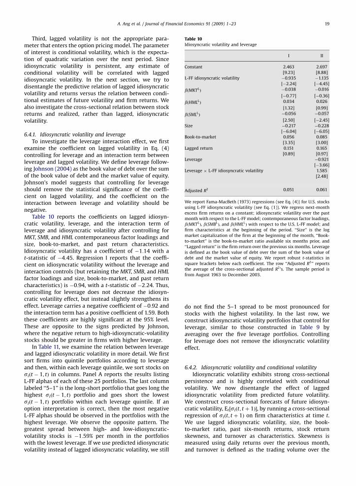
ARTICLE IN PRESS

Table 10Idiosyncratic volatility and leverage

I II

Constant 2.463 2.697

[9.23] [8.88]

L-FF idiosyncratic volatility �0.935 �1.135

[�2.24] [�4.45]

bðMKTLÞ �0.038 �0.016

[�0.77] [�0.36]

bðHMLLÞ 0.034 0.026

[1.32] [0.99]

bðSMLLÞ �0.056 �0.057

[2.50] [�2.45]

Size �0.217 �0.228

[�6.04] [�6.05]

Book-to-market 0.056 0.085

[3.35] [3.00]

Lagged return 0.151 0.165

[0.89] [0.97]

Leverage �0.921

[�3.66]

Leverage � L-FF idiosyncratic volatility 1.585

[2.48]

Adjusted R2 0.051 0.061

We report Fama-MacBeth (1973) regressions (see Eq. (4)) for U.S. stocks

using L-FF idiosyncratic volatility (see Eq. (1)). We regress next-month

excess firm returns on a constant; idiosyncratic volatility over the past

month with respect to the L-FF model; contemporaneous factor loadings,

bðMKTLÞ, bðSMBL

Þ, and bðHMLLÞ with respect to the U.S. L-FF model; and

firm characteristics at the beginning of the period. ‘‘Size’’ is the log

market capitalization of the firm at the beginning of the month, ‘‘Book-

to-market’’ is the book-to-market ratio available six months prior, and

‘‘Lagged return’’ is the firm return over the previous six months. Leverage

is defined as the book value of debt over the sum of the book value of

debt and the market value of equity. We report robust t-statistics in

square brackets below each coefficient. The row ‘‘Adjusted R2’’ reports

the average of the cross-sectional adjusted R2’s. The sample period is

from August 1963 to December 2003.

A. Ang et al. / Journal of Financial Economics 91 (2009) 1–23 19

Third, lagged volatility is not the appropriate para-meter that enters the option pricing model. The parameterof interest is conditional volatility, which is the expecta-tion of quadratic variation over the next period. Sinceidiosyncratic volatility is persistent, any estimate ofconditional volatility will be correlated with laggedidiosyncratic volatility. In the next section, we try todisentangle the predictive relation of lagged idiosyncraticvolatility and returns versus the relation between condi-tional estimates of future volatility and firm returns. Wealso investigate the cross-sectional relation between stockreturns and realized, rather than lagged, idiosyncraticvolatility.

6.4.1. Idiosyncratic volatility and leverage

To investigate the leverage interaction effect, we firstexamine the coefficient on lagged volatility in Eq. (4)controlling for leverage and an interaction term betweenleverage and lagged volatility. We define leverage follow-ing Johnson (2004) as the book value of debt over the sumof the book value of debt and the market value of equity.Johnson’s model suggests that controlling for leverageshould remove the statistical significance of the coeffi-cient on lagged volatility, and the coefficient on theinteraction between leverage and volatility should benegative.

Table 10 reports the coefficients on lagged idiosyn-cratic volatility, leverage, and the interaction term ofleverage and idiosyncratic volatility after controlling forMKT, SMB, and HML contemporaneous factor loadings andsize, book-to-market, and past return characteristics.Idiosyncratic volatility has a coefficient of �1:14 with at-statistic of �4:45. Regression I reports that the coeffi-cient on idiosyncratic volatility without the leverage andinteraction controls (but retaining the MKT, SMB, and HML

factor loadings and size, book-to-market, and past returncharacteristics) is �0:94, with a t-statistic of �2:24. Thus,controlling for leverage does not decrease the idiosyn-cratic volatility effect, but instead slightly strengthens itseffect. Leverage carries a negative coefficient of �0:92 andthe interaction term has a positive coefficient of 1.59. Boththese coefficients are highly significant at the 95% level.These are opposite to the signs predicted by Johnson,where the negative return to high-idiosyncratic-volatilitystocks should be greater in firms with higher leverage.

In Table 11, we examine the relation between leverageand lagged idiosyncratic volatility in more detail. We firstsort firms into quintile portfolios according to leverageand then, within each leverage quintile, we sort stocks onsiðt � 1; tÞ in columns. Panel A reports the results listingL-FF alphas of each of these 25 portfolios. The last columnlabeled ‘‘5–1’’ is the long-short portfolio that goes long thehighest siðt � 1; tÞ portfolio and goes short the lowestsiðt � 1; tÞ portfolio within each leverage quintile. If anoption interpretation is correct, then the most negativeL-FF alphas should be observed in the portfolios with thehighest leverage. We observe the opposite pattern. Thegreatest spread between high- and low-idiosyncratic-volatility stocks is �1:59% per month in the portfolioswith the lowest leverage. If we use predicted idiosyncraticvolatility instead of lagged idiosyncratic volatility, we still

do not find the 5–1 spread to be most pronounced forstocks with the highest volatility. In the last row, weconstruct idiosyncratic volatility portfolios that control forleverage, similar to those constructed in Table 9 byaveraging over the five leverage portfolios. Controllingfor leverage does not remove the idiosyncratic volatilityeffect.

6.4.2. Idiosyncratic volatility and conditional volatility

Idiosyncratic volatility exhibits strong cross-sectionalpersistence and is highly correlated with conditionalvolatility. We now disentangle the effect of laggedidiosyncratic volatility from predicted future volatility.We construct cross-sectional forecasts of future idiosyn-cratic volatility, Et½siðt; t þ 1Þ�, by running a cross-sectionalregression of siðt; t þ 1Þ on firm characteristics at time t.We use lagged idiosyncratic volatility, size, the book-to-market ratio, past six-month returns, stock returnskewness, and turnover as characteristics. Skewness ismeasured using daily returns over the previous month,and turnover is defined as the trading volume over the

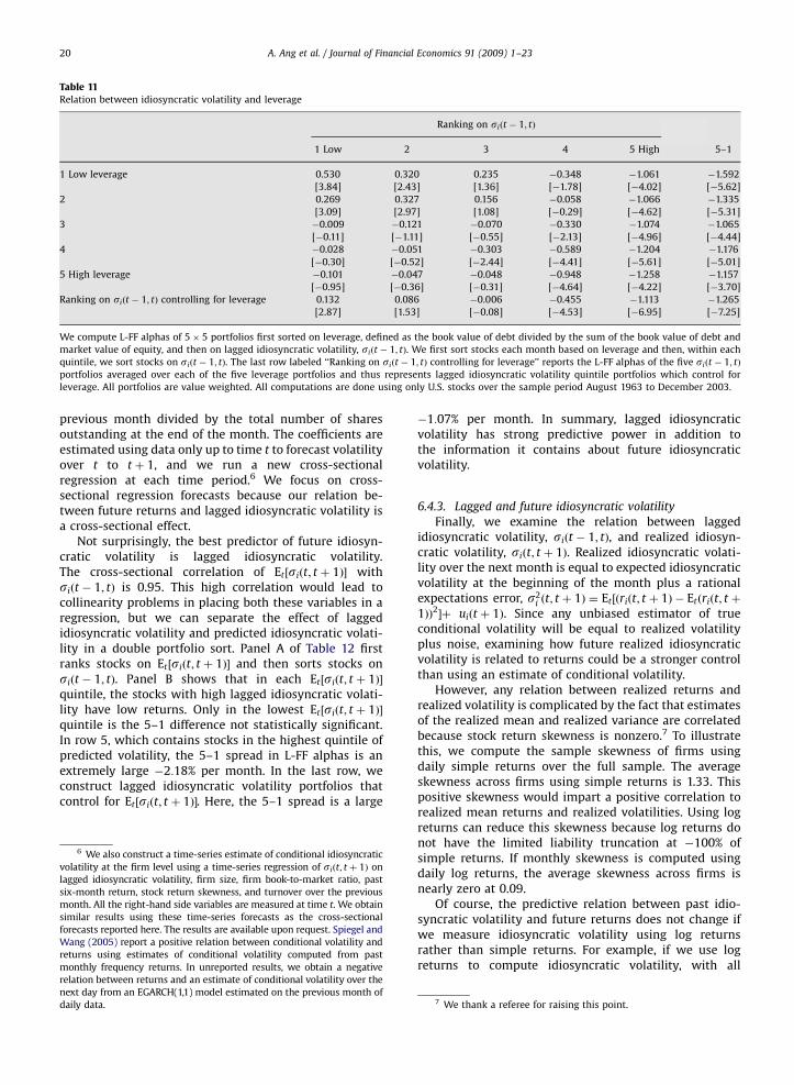
ARTICLE IN PRESS

Table 11Relation between idiosyncratic volatility and leverage

Ranking on siðt � 1; tÞ

1 Low 2 3 4 5 High 5–1

1 Low leverage 0.530 0.320 0.235 �0.348 �1.061 �1.592

[3.84] [2.43] [1.36] [�1.78] [�4.02] [�5.62]

2 0.269 0.327 0.156 �0.058 �1.066 �1.335

[3.09] [2.97] [1.08] [�0.29] [�4.62] [�5.31]

3 �0.009 �0.121 �0.070 �0.330 �1.074 �1.065

[�0.11] [�1.11] [�0.55] [�2.13] [�4.96] [�4.44]

4 �0.028 �0.051 �0.303 �0.589 �1.204 �1.176

[�0.30] [�0.52] [�2.44] [�4.41] [�5.61] [�5.01]

5 High leverage �0.101 �0.047 �0.048 �0.948 �1.258 �1.157

[�0.95] [�0.36] [�0.31] [�4.64] [�4.22] [�3.70]

Ranking on siðt � 1; tÞ controlling for leverage 0.132 0.086 �0.006 �0.455 �1.113 �1.265

[2.87] [1.53] [�0.08] [�4.53] [�6.95] [�7.25]

We compute L-FF alphas of 5� 5 portfolios first sorted on leverage, defined as the book value of debt divided by the sum of the book value of debt and

market value of equity, and then on lagged idiosyncratic volatility, siðt � 1; tÞ. We first sort stocks each month based on leverage and then, within each

quintile, we sort stocks on siðt � 1; tÞ. The last row labeled ‘‘Ranking on siðt � 1; tÞ controlling for leverage’’ reports the L-FF alphas of the five siðt � 1; tÞ

portfolios averaged over each of the five leverage portfolios and thus represents lagged idiosyncratic volatility quintile portfolios which control for

leverage. All portfolios are value weighted. All computations are done using only U.S. stocks over the sample period August 1963 to December 2003.

A. Ang et al. / Journal of Financial Economics 91 (2009) 1–2320

previous month divided by the total number of sharesoutstanding at the end of the month. The coefficients areestimated using data only up to time t to forecast volatilityover t to t þ 1, and we run a new cross-sectionalregression at each time period.6 We focus on cross-sectional regression forecasts because our relation be-tween future returns and lagged idiosyncratic volatility isa cross-sectional effect.

Not surprisingly, the best predictor of future idiosyn-cratic volatility is lagged idiosyncratic volatility.The cross-sectional correlation of Et½siðt; t þ 1Þ� withsiðt � 1; tÞ is 0.95. This high correlation would lead tocollinearity problems in placing both these variables in aregression, but we can separate the effect of laggedidiosyncratic volatility and predicted idiosyncratic volati-lity in a double portfolio sort. Panel A of Table 12 firstranks stocks on Et ½siðt; t þ 1Þ� and then sorts stocks onsiðt � 1; tÞ. Panel B shows that in each Et½siðt; t þ 1Þ�quintile, the stocks with high lagged idiosyncratic volati-lity have low returns. Only in the lowest Et½siðt; t þ 1Þ�quintile is the 5–1 difference not statistically significant.In row 5, which contains stocks in the highest quintile ofpredicted volatility, the 5–1 spread in L-FF alphas is anextremely large �2:18% per month. In the last row, weconstruct lagged idiosyncratic volatility portfolios thatcontrol for Et½siðt; t þ 1Þ�. Here, the 5–1 spread is a large

6 We also construct a time-series estimate of conditional idiosyncratic

volatility at the firm level using a time-series regression of siðt; t þ 1Þ on

lagged idiosyncratic volatility, firm size, firm book-to-market ratio, past

six-month return, stock return skewness, and turnover over the previous

month. All the right-hand side variables are measured at time t. We obtain

similar results using these time-series forecasts as the cross-sectional

forecasts reported here. The results are available upon request. Spiegel and

Wang (2005) report a positive relation between conditional volatility and

returns using estimates of conditional volatility computed from past

monthly frequency returns. In unreported results, we obtain a negative

relation between returns and an estimate of conditional volatility over the

next day from an EGARCH(1,1) model estimated on the previous month of

daily data.

�1:07% per month. In summary, lagged idiosyncraticvolatility has strong predictive power in addition tothe information it contains about future idiosyncraticvolatility.

6.4.3. Lagged and future idiosyncratic volatility

Finally, we examine the relation between laggedidiosyncratic volatility, siðt � 1; tÞ, and realized idiosyn-cratic volatility, siðt; t þ 1Þ. Realized idiosyncratic volati-lity over the next month is equal to expected idiosyncraticvolatility at the beginning of the month plus a rationalexpectations error, s2

i ðt; t þ 1Þ ¼ Et½ðriðt; t þ 1Þ � Etðriðt; t þ

1ÞÞ2�þ uiðt þ 1Þ. Since any unbiased estimator of trueconditional volatility will be equal to realized volatilityplus noise, examining how future realized idiosyncraticvolatility is related to returns could be a stronger controlthan using an estimate of conditional volatility.

However, any relation between realized returns andrealized volatility is complicated by the fact that estimatesof the realized mean and realized variance are correlatedbecause stock return skewness is nonzero.7 To illustratethis, we compute the sample skewness of firms usingdaily simple returns over the full sample. The averageskewness across firms using simple returns is 1.33. Thispositive skewness would impart a positive correlation torealized mean returns and realized volatilities. Using logreturns can reduce this skewness because log returns donot have the limited liability truncation at �100% ofsimple returns. If monthly skewness is computed usingdaily log returns, the average skewness across firms isnearly zero at 0.09.

Of course, the predictive relation between past idio-syncratic volatility and future returns does not change ifwe measure idiosyncratic volatility using log returnsrather than simple returns. For example, if we use logreturns to compute idiosyncratic volatility, with all

7 We thank a referee for raising this point.

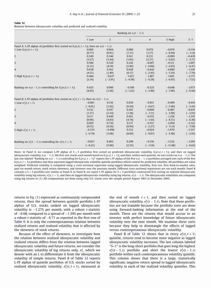
ARTICLE IN PRESS

Table 12Relation between idiosyncratic volatility and predicted and realized volatility

Ranking on siðt � 1; tÞ

1 Low 2 3 4 5 High 5–1

Panel A: L-FF alphas of portfolios first sorted on Et ½siðt; t þ 1Þ�, then on siðt � 1; tÞ

1 Low Et ½siðt; t þ 1Þ� 0.069 0.064 0.089 0.079 �0.070 �0.139

[0.77] [0.91] [1.31] [1.17] [�0.94] [�1.14]

2 0.349 0.346 0.161 0.231 �0.089 �0.438

[3.57] [3.44] [1.65] [2.27] [�0.92] [�3.17]

3 0.586 0.520 0.242 �0.007 �0.511 �1.097

[5.12] [4.19] [2.09] [�0.06] [�4.03] [�6.47]

4 0.638 0.183 0.028 �0.442 �0.880 �1.518

[4.51] [1.40] [0.17] [�2.95] [�5.19] [�7.70]

5 High Et ½siðt; t þ 1Þ� 0.484 �0.617 �1.021 �1.487 �1.691 �2.175

[2.14] [�2.91] [�4.58] [�6.28] [�6.45] [�7.52]

Ranking on siðt � 1; tÞ controlling for Et ½siðt; t þ 1Þ� 0.425 0.099 �0.100 �0.325 �0.648 �1.073

[4.95] [1.26] [�1.22] [�3.90] [�7.09] [�9.44]

Panel B: L-FF alphas of portfolios first sorted on sLi ðt; t þ 1Þ, then on sL

i ðt � 1; tÞ

1 Low sLi ðt; t þ 1Þ �0.081 0.136 0.036 �0.051 �0.490 �0.410

[�0.91] [1.92] [0.50] [�0.67] [�5.90] [�3.43]

2 0.132 0.197 0.105 �0.099 �0.487 �0.619

[1.57] [2.54] [1.38] [�1.11] [�3.99] [�3.93]

3 0.117 0.449 0.451 �0.155 �1.218 �1.335

[0.96] [4.83] [4.74] [�1.43] [�8.31] [�6.36]

4 0.029 0.736 0.137 �0.351 �2.094 �2.122

[0.13] [4.56] [0.94] [�2.27] [�11.4] [�7.58]

5 High sLi ðt; t þ 1Þ �0.333 �0.496 0.312 �0.024 �1.870 �1.537

[�0.74] [1.68] [0.94] [�0.07] [�5.48] [�2.95]

Ranking on sLi ðt � 1; tÞ controlling for sL

i ðt; t þ 1Þ �0.027 0.403 0.208 �0.136 �1.232 �1.205

[�0.21] [5.06] [2.53] [�1.54] [�11.48] [�6.63]

Notes: In Panel A, we compute L-FF alphas of 5� 5 portfolios first sorted on predicted idiosyncratic volatility, Et ½siðt; t þ 1Þ�, and then on lagged

idiosyncratic volatility, siðt � 1; tÞ. We first sort stocks each month based on Et ½siðt; t þ 1Þ�, and then, within each quintile, we sort stocks on siðt � 1; tÞ. The

last row labeled ‘‘Ranking on siðt � 1; tÞ controlling for Et ½siðt; t þ 1Þ�’’ reports the L-FF alphas of the five siðt � 1; tÞ portfolios averaged over each of the five

Et ½siðt; t þ 1Þ� portfolios and thus represent lagged idiosyncratic volatility quintile portfolios which control for predicted volatility. All portfolios are value

weighted. Predicted volatility is computed using a cross-sectional regression using lagged idiosyncratic volatility, firm size, firm book-to-market ratio,

past six-month return, stock return skewness, and turnover over the previous month. Different cross-sectional regressions are run each month. Panel B

contains a 5� 5 portfolio sort similar to Panel A. In Panel B, we report L-FF alphas for 5� 5 portfolios constructed first sorting on realized idiosyncratic

volatility using log returns, sLi ðt; t þ 1Þ, and then on lagged idiosyncratic volatility using log returns, sL

i ðt � 1; tÞ. The idiosyncratic volatilities are computed

using log returns in (1). All computations are done using only U.S. stocks over the sample period August 1963 to December 2003.

A. Ang et al. / Journal of Financial Economics 91 (2009) 1–23 21

returns in Eq. (1) expressed as continuously compoundedreturns, then the spread between quintile portfolio L-FFalphas of U.S. stocks ranked on lagged idiosyncraticvolatility is �1:27% per month, with a robust t-statisticof �6:68, compared to a spread of �1:29% per month witha robust t-statistic of �6:71 as reported in the first row ofTable 9. It is only the contemporaneous relation betweenrealized returns and realized volatility that is affected bythe skewness of stock returns.

Because of the effect of skewness, to investigate howthe relation between realized idiosyncratic volatility andrealized returns differs from the relation between laggedidiosyncratic volatility and future returns, we consider theidiosyncratic volatility of log returns only, sL

i , which wedenote with an L to differentiate it from the idiosyncraticvolatility of simple returns. Panel B of Table 12 reportsL-FF alphas of quintile portfolios of U.S. stocks sorted byrealized idiosyncratic volatility, sL

i ðt; t þ 1Þ, measured at

the end of month t þ 1, and then sorted on laggedidiosyncratic volatility, sL

i ðt � 1; tÞ. Note that these portfo-lios are not tradable because the portfolio sorts are doneusing forward-looking information at the end of themonth. These are the returns that would accrue to aninvestor with perfect knowledge of future idiosyncraticvolatility over the next month. We examine these sortsbecause they help to disentangle the effects of laggedversus contemporaneous idiosyncratic volatility.

Panel B of Table 12 shows that in every sLi ðt; t þ 1Þ

quintile, returns tend to become more negative as laggedidiosyncratic volatility increases. The last column labeled‘‘5–1’’ is the long-short portfolio that goes long the highestsL

i ðt � 1; tÞ portfolio and short the lowest sLi ðt � 1; tÞ

portfolio within each contemporaneous volatility quintile.This column shows that there is a large, statisticallysignificant, negative return spread to lagged idiosyncraticvolatility in each of the realized volatility quintiles. This

ARTICLE IN PRESS

A. Ang et al. / Journal of Financial Economics 91 (2009) 1–2322

5–1 spread ranges from �0:41% per month for the firstsL

i ðt; t þ 1Þ quintile portfolio to a very large �2:12% in thefourth sL

i ðt; t þ 1Þ quintile portfolio.In the last row of Panel B, we report L-FF alphas of

quintile portfolios of sLi ðt � 1; tÞ controlling for the effect

of contemporaneous volatility. Controlling for contem-poraneous idiosyncratic volatility, the 5–1 return spread isa large �1:21% per month, which is highly significant witha t-statistic of �6:63. Thus, future exposure to highidiosyncratic volatility does not explain why the rewardsto holding stocks with low past idiosyncratic volatility areso low.

7. Conclusion

Around the world, stocks with recent past highidiosyncratic volatility tend to have much lower returnsthan stocks with recent past low idiosyncratic volatility.We measure idiosyncratic volatility with respect to local,regional, or world versions of the Fama and French (1993,1998) factor model. After sorting stocks across 23countries on past idiosyncratic volatility, the differencein alphas adjusting for market, size, and book-to-marketfactors between stocks in the highest quintile of idiosyn-cratic volatility and stocks in the lowest quintile ofidiosyncratic volatility is a very large �1:31% per month.This effect is also strongly statistically significant. Theselow returns to high-idiosyncratic-volatility stocks simul-taneously appear in different world regions and are robustto controlling for additional factor loadings and firmcharacteristics. Since these results are out-of-samplerelative to the earlier U.S. findings of Ang, Hodrick, Xing,and Zhang (2006), the implication is that the relationbetween high idiosyncratic volatility and low returns isnot just a sample-specific or country-specific effect but isobserved worldwide.

We find that the low returns earned by stocks withhigh idiosyncratic volatility around the world co-movesignificantly with the idiosyncratic volatility effect in theUnited States. In particular, after controlling for U.S.portfolios comprising long positions in stocks with highidiosyncratic volatilities and short positions in stocks withlow idiosyncratic volatilities, the alphas of portfoliostrategies trading the idiosyncratic volatility effect invarious international markets are insignificant. Thus, theglobal idiosyncratic volatility effect is captured by asimple U.S. idiosyncratic volatility factor. In contrast, thelow returns of high idiosyncratic stocks in internationalmarkets cannot be explained by standard factors or riskloadings.

However, we are hesitant to claim that the low returnsto high-idiosyncratic-volatility stocks results from expo-sure to systematic risk. In further analysis on U.S. data, werule out complete explanations based on trading orclientele structures, higher moments, and informationdissemination. The low returns of stocks with past highidiosyncratic volatility cannot be explained by the lever-age interaction story of Johnson (2004) or by futureexposure to idiosyncratic volatility. Our strong interna-tional results suggest that market-specific stories are also

unlikely to hold. We conclude that the puzzle of lowreturns to high-idiosyncratic-volatility stocks have lowreturns is a global phenomenon. Further research mustinvestigate if there are true economic sources of riskbehind the idiosyncratic volatility phenomenon causingstocks with high volatility to have low expected returns.

References

Adrian, T., Rosenberg, J., 2007. Stock returns and volatility: pricing theshort-run and long-run components of market risk. Journal ofFinance, forthcoming.

Ang, A., Hodrick, R.J., Xing, Y., Zhang, X., 2006. The cross-section ofvolatility and expected returns. Journal of Finance 51, 259–299.

Baker, M., Coval, J., Stein, J.C., 2007. Corporate financing decisions wheninvestors take the path of least resistance. Journal of FinancialEconomics 84, 266–298.

Bali, T., Cakici, N., 2008. Idiosyncratic risk and the cross-section ofexpected returns. Journal of Financial and Quantitative Analysis 43,29–58.

Bali, T., Cakici, N., Yan, X., Zhang, Z., 2005. Does idiosyncratic volatilityreally matter? Journal of Finance 60, 905–929.

Banz, R.W., 1981. The relationship between return and market value ofcommon stocks. Journal of Financial Economics 9, 3–18.

Barberis, N., Huang, M., 2005. Stocks as lotteries: the implications ofprobability weighting for security prices. Unpublished workingpaper, Yale University.

Bekaert, G., Hodrick, R.J., Zhang, X., 2005. International stock returncomovements. Unpublished working paper, Cornell University.

Black, F., Scholes, M.S., 1973. The pricing of options and corporateliabilities. Journal of Political Economy 81, 637–659.

Black, F., Jensen, M., Scholes, M.S., 1972. The capital asset pricing model:some empirical tests. In: Jensen, M. (Ed.), Studies in the Theory ofCapital Markets. Praeger, New York, pp. 79–121.

Brandt, M.W., Brav, A., Graham, J.R., 2005. The idiosyncratic volatilitypuzzle: time trend or speculative episodes? Unpublished workingpaper, Duke University.

Brennan, M., Subrahmanyam, A., 1995. Investment analysis and priceformation in securities markets. Journal of Financial Econometrics38, 361–381.

Brooks, R., Del Negro, M., 2005. Country versus region effects ininternational stock returns. Journal of Portfolio Management 31,67–72.

Brown, D.P., Ferreira, M.A., 2003. Information in the idiosyncraticvolatility of small firms. Unpublished working paper, ISCTE BusinessSchool.

Campbell, J.Y., 1993. Intertemporal asset pricing without consumptiondata. American Economic Review 83, 487–512.

Campbell, J.Y., Lettau, M., Malkiel, B.G., Xu, Y., 2001. Have individualstocks become more volatile? An empirical exploration of idiosyn-cratic risk. Journal of Finance 56, 1–44.

Chordia, T., Huh, S.W., Subrahmanyam, A., 2007. The cross-section ofexpected trading activity. Review of Financial Studies 20, 709–740.

Daniel, K., Titman, S., 1997. Evidence on the characteristics of crosssectional variation in stock returns. Journal of Finance 52, 1–33.

Diether, K.B., Malloy, C.J., Scherbina, A., 2002. Differences of opinion andthe cross section of stock returns. Journal of Finance 57, 2113–2141.

Easley, D., O’Hara, M., 2004. Information and the cost of capital. Journalof Finance 59, 1553–1583.

Easley, D., Hvidkjaer, S., O’Hara, M., 2002. Is information risk adeterminant of asset returns? Journal of Finance 57, 2185–2221.

Engle, R.F., 1982. Autoregressive conditional heteroscedasticity withestimates of the variance of United Kingdom inflation. Econometrica50, 987–1008.

Fama, E.F., French, K.R., 1992. The cross-section of expected stock returns.Journal of Finance 47, 427–465.

Fama, E.F., French, K.R., 1993. Common risk factors in the returns onstocks and bonds. Journal of Financial Economics 33, 3–56.

Fama, E.F., French, K.R., 1998. Value versus growth: the internationalevidence. Journal of Finance 53, 1975–1999.

Fama, E.F., MacBeth, J.D., 1973. Risk, return, and equilibrium: empiricaltests. Journal of Political Economy 71, 607–636.

Fu, F., 2005. Idiosyncratic risk and the cross-section of expected stockreturns. Unpublished working paper, University of Rochester.

Goyal, A., Santa-Clara, P., 2003. Idiosyncratic risk matters!. Journal ofFinance 58, 975–1007.

ARTICLE IN PRESS

A. Ang et al. / Journal of Financial Economics 91 (2009) 1–23 23

Guo, H., Savickas, R., 2007. Aggregate idiosyncratic volatility in G7countries. Review of Financial Studies, forthcoming.

Harvey, C.R., Siddique, A., 2000. Conditional skewness in asset pricingtests. Journal of Finance 55, 1263–1295.

Heston, S.L., 1993. A closed-form solution for options with stochasticvolatility with applications to bond and currency options. Review ofFinancial Studies 6, 327–343.

Hong, H., Lim, T., Stein, J.C., 2000. Bad news travels slowly: size, analystcoverage, and the profitability of momentum strategies. Journal ofFinance 55, 265–295.

Hou, K.W., Moskowitz, T., 2005. Market frictions, price delay, and thecross-section of expected returns. Review of Financial Studies 18,981–1020.

Huang, W., Liu, Q., Rhee, G., Zhang, L., 2006. Another look at idiosyncraticrisk and expected returns. Unpublished working paper, University ofHawaii at Manoa.

Jagannathan, R., Wang, Z., 1996. The conditional CAPM and the cross-section of expected returns. Journal of Finance 51, 3–53.

Jegadeesh, N., Titman, S., 1993. Returns to buying winners and sellinglosers: implications for stock market efficiency. Journal of Finance48, 65–92.

Jiang, G.J., Xu, D., Yao, T., 2005. The information content of idiosyncraticvolatility. Journal of Financial and Quantitative Analysis, forth-coming.

Johnson, T., 2004. Forecast dispersion and the cross section of expectedreturns. Journal of Finance 59, 1957–1978.

Kumar, A., 2007. Who gambles in the stock market? Unpublishedworking paper, University of Texas at Austin.

Ledoit, O., Santa-Clara, P., Yan, S., 2002. Relative pricing of options withstochastic volatility. Unpublished working paper, UCLA.

Lesmond, D.A., Ogden, J.P., Trzcinka, C.A., 1999. A new estimate oftransaction costs. Review of Financial Studies 12, 1113–1141.

Lo, A.W., MacKinlay, A.C., 1990. Data-snooping biases in tests offinancial asset pricing models. Review of Financial Studies 3,431–467.

Merton, R.C., 1974. On the pricing of corporate debt: the risk structure ofinterest rates. Journal of Finance 29, 449–470.

Merton, R.C., 1987. Presidential address: a simple model of capital marketequilibrium with incomplete information. Journal of Finance 42,483–510.

Miller, E., 1977. Risk, uncertainty and divergence of opinion. Journal ofFinance 32, 1151–1168.

Newey, W.K., West, K.D., 1987. A simple positive semi-definite, hetero-skedasticity and autocorrelation consistent covariance matrix.Econometrica 55, 703–708.

Rouwenhorst, K.G., 1998. International momentum strategies. Journal ofFinance 53, 267–284.

Shanken, J., 1992. On the estimation of beta pricing models. Review ofFinancial Studies 5, 1–34.

Spiegel, M., Wang, X., 2005. Cross-sectional variation in stock returns:liquidity and idiosyncratic risk. Unpublished working paper, YaleUniversity.

Tversky, A., Kahneman, D., 1992. Advances in prospect theory: cumula-tive representation of uncertainty. Journal of Risk and Uncertainty 5,297–323.

Wei, S., Zhang, C., 2005. Idiosyncratic volatility does not matter: a re-examination of the relation between average returns and averagevolatilities. Journal of Banking and Finance 29, 603–621.

Zhang, X.F., 2006. Information uncertainty and stock returns. Journal ofFinance 61, 105–135.