HIPEAC 2018 Conference

Proceedings of

RAPDIO 2018 Workshop

Manchester, United Kingdom

22th January 2018

I

Organizing committee

Daniel Chillet, University of Rennes 1Reda Nouacer, CEA List

Morteza Biglari-Abhari, University of AucklandDaniel Gracia Perez, Thales Research & Technology

Gianluca Palermo, Politecnico di Milano

Program committee

Mario Porrmann, Bielefeld UniversityRoberto Giorgi, University of Siena

Philipp A. Hartmann, IntelJeronimo Castrillon, TU Dresden

Sotirios Xydis, National Technical University of AthensMichael Huebner, Ruhr-University Bochum

Tim Kogel, SynopsysFrederic Petrot, TIMA Lab, Grenoble Institute of Technology

Antonino Tumeo, Politecnico di MilanoPierre Boulet, Univ Lille 1, CRIStALDavide Quaglia, University of Verona

Christian Haubelt, University of RostockAlper Sen, Bogazici University

Website

http://www.rapido.deib.polimi.it

http://www.rapido.deib.polimi.it/RapidoProceedings.pdf

II

Schedule

— Session 1 10 : 00− 11 : 00— Keynote 1 Nikil Dutt, University of California, Irvine

Self-Awareness for Heterogeneous MPSoCs : A Case Study using Adaptive, Reflec-tive Middleware

— Session 2 11 : 15− 12 : 45— Keynote 2 Tim Kogel, Synopsys

Building Smart SoCs - Using Virtual Prototyping for the Design of SoCs withArtificial Intelligence Accelerators

— Rabab Bouziane, Erven Rohou and Abdoulaye GamatieCompile-Time Silent Store Elimination for Energy Efficiency : an Analytic Eva-luation for Non-Volatile Cache Memory

— Gereon Onnebrink, Rainer Leupers and Gerd AscheidESL Black Box Power Estimation : Automatic Calibration for IEEE UPF 3.0 Po-wer Models

— Session 3 14 : 00− 15 : 30— Keynote 3 Alberto Bosio, Lirmm, Montpellier, France

Cross-Layer system-level reliability Estimation— Giovanni Liboni, Julien Deantoni, Antonio Portaluri, Davide Quaglia and Robert

De SimoneBeyond Time-Triggered Co-simulation of Cyber-Physical Systems for Performanceand Accuracy Improvements

— Ahmet Erdem, Davide Gadioli, Gianluca Palermo and Cristina SilvanoDesign Space Pruning and Computational Workload Splitting for Autotuning OpenCLApplications

— Vittoriano Muttillo, Giacomo Valente, Daniele Ciambrone, Vincenzo Stoico andLuigi PomanteHEPSYCODE-RT : a Real-Time Extension for an ESL HW/SW Co-Design Me-thodology

— Session 4 16 : 00− 17 : 30— Keynote 4 Guy Bois, Polytechnique Montreal and President of Space Codesign

SystemsSpecific needs for the modelling and the refinement of CPU and FPGA platforms

— Irune Yarza, Mikel Azkarate-Askasua, Kim Gruttner and Wolfgang NebelReal-Time Capable Retargeting of Xilinx MicroBlaze Binaries using QEMU

— Asif Ali Khan, Fazal Hameed and Jeronimo CastrillonNVMain Extension for Multi-Level Cache Systems

— Alexandre Chabot, Ihsen Alouani, Smail Niar and Reda NouacerA Fault Injection Platform for Early-Stage Reliability Assessment

III

List of regular papers

ESL Black Box Power Estimation : Automatic Calibration for IEEE UPF 3.0 Power Models,Gereon Onnebrink, Rainer Leupers and Gerd Ascheid

Beyond Time-Triggered Co-simulation of Cyber-Physical Systems for Performance and Ac-curacy Improvements, Giovanni Liboni, Julien Deantoni, Antonio Portaluri, Davide Quagliaand Robert De Simone

Real-Time Capable Retargeting of Xilinx MicroBlaze Binaries using QEMU, Irune Yarza,Mikel Azkarate-Askasua, Kim Gruttner and Wolfgang Nebel

Design Space Pruning and Computational Workload Splitting for Autotuning OpenCL Appli-cations, Ahmet Erdem, Davide Gadioli, Gianluca Palermo and Cristina Silvano

Compile-Time Silent Store Elimination for Energy Efficiency : an Analytic Evaluation forNon-Volatile Cache Memory, Rabab Bouziane, Erven Rohou and Abdoulaye Gamatie

HEPSYCODE-RT : a Real-Time Extension for an ESL HW/SW Co-Design Methodology,Vittoriano Muttillo, Giacomo Valente, Daniele Ciambrone, Vincenzo Stoico and Luigi Po-mante

NVMain Extension for Multi-Level Cache Systems, Asif Ali Khan, Fazal Hameed and Jero-nimo Castrillon

Work in progress paper

Fault Injection Platform for Early-Stage Reliability Assessment, Alexandre Alexandre Cha-bot, Ihsen Alouani, Smail Niar and Reda Nouacer

IV

ESL Black Box Power Estimation :Automatic Calibration for IEEEUPF 3.0 Power Models

V

ESL Black Box Power Estimation: Automatic Calibration forIEEE UPF 3.0 Power Models

Gereon OnnebrinkInstitute for Communication

Technologies and Embedded SystemsRWTH Aachen University, Germany

onnebrink@ice.rwth-aachen.de

Rainer LeupersInstitute for Communication

Technologies and Embedded SystemsRWTH Aachen University, Germany

leupers@ice.rwth-aachen.de

Gerd AscheidInstitute for Communication

Technologies and Embedded SystemsRWTH Aachen University, Germany

ascheid@ice.rwth-aachen.de

ABSTRACTPower-aware design space exploration at early electronic systemlevel (ESL) is highly facilitated by virtual platforms. In order todefine and exchange power models, the IEEE standard 1801-2015 –UPF has been defined to allow developers, vendors and customersseamless usage of the same power models. However, one obstacleis still not covered by the standard: it is not specified and solvedhow to construct the model in the first place. This paper offersa solution to close this gap. A well proven semi-automatic blackbox ESL power estimation methodology [17], which allows to havepower estimates with approximately 5 % error, is combined withUPF. Although the standard is based on power state machinesand requires another tracing method, a procedure is presented toovercome these differences. Representative case studies show thatsimilar estimation accuracy can be achieved.

CCS CONCEPTS• Hardware → Power estimation and optimization; Electronicdesign automation; • Computing methodologies → Modelingmethodologies; • General and reference →Measurement;

KEYWORDSElectronic system level, power model, power estimation, digitalsignal processor

ACM Reference Format:Gereon Onnebrink, Rainer Leupers, and Gerd Ascheid. 2018. ESL Black BoxPower Estimation: Automatic Calibration for IEEE UPF 3.0 Power Models. InRAPIDO: Rapid Simulation and Performance Evaluation: Methods and Tools,January 22–24, 2018, Manchester, United Kingdom. ACM, New York, NY,USA, 6 pages. https://doi.org/10.1145/3180665.3180667

1 INTRODUCTIONThe ever increasing computational workloads and tighter con-straints, such as power budget, battery lifetime and sufficient perfor-mance, have to be tackled by the next generation of MultiprocessorSystems-on-Chip (MPSoCs). To provide the best trade-off between

Permission to make digital or hard copies of all or part of this work for personal orclassroom use is granted without fee provided that copies are not made or distributedfor profit or commercial advantage and that copies bear this notice and the full citationon the first page. Copyrights for components of this work owned by others than ACMmust be honored. Abstracting with credit is permitted. To copy otherwise, or republish,to post on servers or to redistribute to lists, requires prior specific permission and/or afee. Request permissions from permissions@acm.org.RAPIDO, January 22–24, 2018, Manchester, United Kingdom© 2018 Association for Computing Machinery.ACM ISBN 978-1-4503-6417-1/18/01. . . $15.00https://doi.org/10.1145/3180665.3180667

cost, power and performance, these platforms generally incorpo-rate diverse processing elements, e.g., general purpose processors,DSPs and GPUs, along with target application optimised commu-nication network topologies and memories. Short time-to-marketcycles bear huge challenges to the Design Space Exploration (DSE)of such complex MPSoCs. While most accurate values for powerconsumption and performance can only be gathered at late stagesof the design flow, design decisions made at Electronic System Level(ESL) have a much stronger impact [25].

Virtual Platforms (VPs) enable hardware and software co-design.The industry standard approach is to use SystemC TransactionLevel Modelling (TLM) [3] for DSE at ESL. On the one hand, timingsimulation is a stable feature and can be set from cycle accurateover instruction accurate to pure functional simulation to fit theneed of the MPSoC designer. On the other hand, power estimationis still under development. Academia has proposed many differentapproaches how power-aware simulations at ESL can be achieved.Some of them have already been adopted and shipped in industrystandard tools. To further unify the community, a common way ofbuilding and exchanging power models for all components of anMPSoC is required. Usually, IP vendors want to give such models totheir customers or share them internally. The former usually impliesthat the component model is shipped as binary code, i.e. black box.Hence, less inputs are available to drive a shareable power model.Therefore, the IEEE standard 1801-2015 was extended to provide aninterface [2]. In its current version 3.0, the Unified Power Format(UPF) supports SystemC TLM VPs and uses Power State Machines(PSMs) as a reasonable modelling approach for highly accuratepower estimates (cf. Section 3.2).

Unfortunately, the standard lacks one important detail. There isno definition or procedure how a power model can be constructedin the first place. In general, an indispensable requirement is theneed of a reference in form of spreadsheets, lower level simulationsfrom previous design cycles or even hardware measurements. Besi-des that, a method of calibrating the UPF power model with thisreference is strongly desired. To close this gap, this paper proposesan extension for the well proven ESL black box power estimationmethodology, presented in [17]. In order to enable automatic powermodel calibration for UPF, the following contributions are presen-ted:

• Extending the ESL black box power estimation method tosupport tracing of UPF relevant states.

• Generating PSM power models out of the ESL power estima-tion methodology approach automatically.

• Evaluation of the proposed methodology for ARMCortex-A9and Blackfin 609 DSP processors.

RAPIDO, January 22–24, 2018, Manchester, United Kingdom Gereon Onnebrink, Rainer Leupers, and Gerd Ascheid

• Comparison with an industry standard tool that supportsUPF power models.

2 RELATEDWORKOver the last decade, intensive research has been conducted in in-dustry and academia to find solutions for power-aware DSE at ESL.Three industry standard tools are the Virtualizer tool set from Syn-opsys [23], Aceplorer from Intel Docea [1], and Vista from MentorGraphics [25].

Trying to enable fast and power-aware system level simulationsis already done in early work by using equations or table basedpower models for each single instruction with a cycle accuratearchitectural simulator [5, 6, 27]. More recent work adopts thistechnique and enables it for cycle [21] and fast instruction-accurateSystemC simulations [19]. The concept of functional level poweranalysis (FLPA) is a more abstracted variant and presented in [13].Using FLPA, a power model is built for every functional unit. Newerwork combines FLPAwith SystemC simulations and extends it fromprocessor models to the entire MPSoC platform, e.g. models forcaches. Measurement on real hardware is performed as calibrationreference for each functional unit [12, 16].

Another approach to build power models is to use finite state ma-chines, so called PSMs. Such a PSM can be driven from a functionalSystemC simulation [22]. Possible covered states are active and idlepower, and dynamic voltage and frequency scaling affected states.The works [7, 9] make use of the TLM time annotation style andthe extension mechanism of TLM to implement and drive the PSMs.There is also work that relies on an older version of the IEEE-1801standard [4]. But the question how to generate reasonable powerstates is not answered.

Besides power models for processors, investigations are con-ducted with focus on memory and communication networks ofMPSoCs. A power model has been built for a specific 3D-DRAMsystem in [11]. A data sheet serves as input for the power valuesand the simulation of the DRAM control commands gives the ac-tual timing behaviour. This procedure is formalised with Petri Netsin [10]. Looking into communication architectures, a frameworkthat deals with bus matrices is introduced in [15] and uses energymacro models to obtain the power and energy consumption. Alinear combination of RTL signal traces is linked into SystemCTLM modules to estimate power and energy. Generating powermodels in a similar way, different communication architectures areinvestigated in [18]. A semi-automatic curve-fitting approach isused to calibrate the power models from ESL traces and a reference,such as measurements of actual hardware or simulation at lowerabstraction levels.

All previously mentioned approaches have in common that thepower model has to be obtained in the first place, but except theapproach of [18], no generic applicable method is given. Further,insight into the models is necessary to drive the power estimation.To overcome the latter, a black box power estimation methodologyis presented and evaluated in [14, 17]. The contributions of thesethree works are the basis of this work, where a semi-automaticgeneration of UPF power models is proposed.

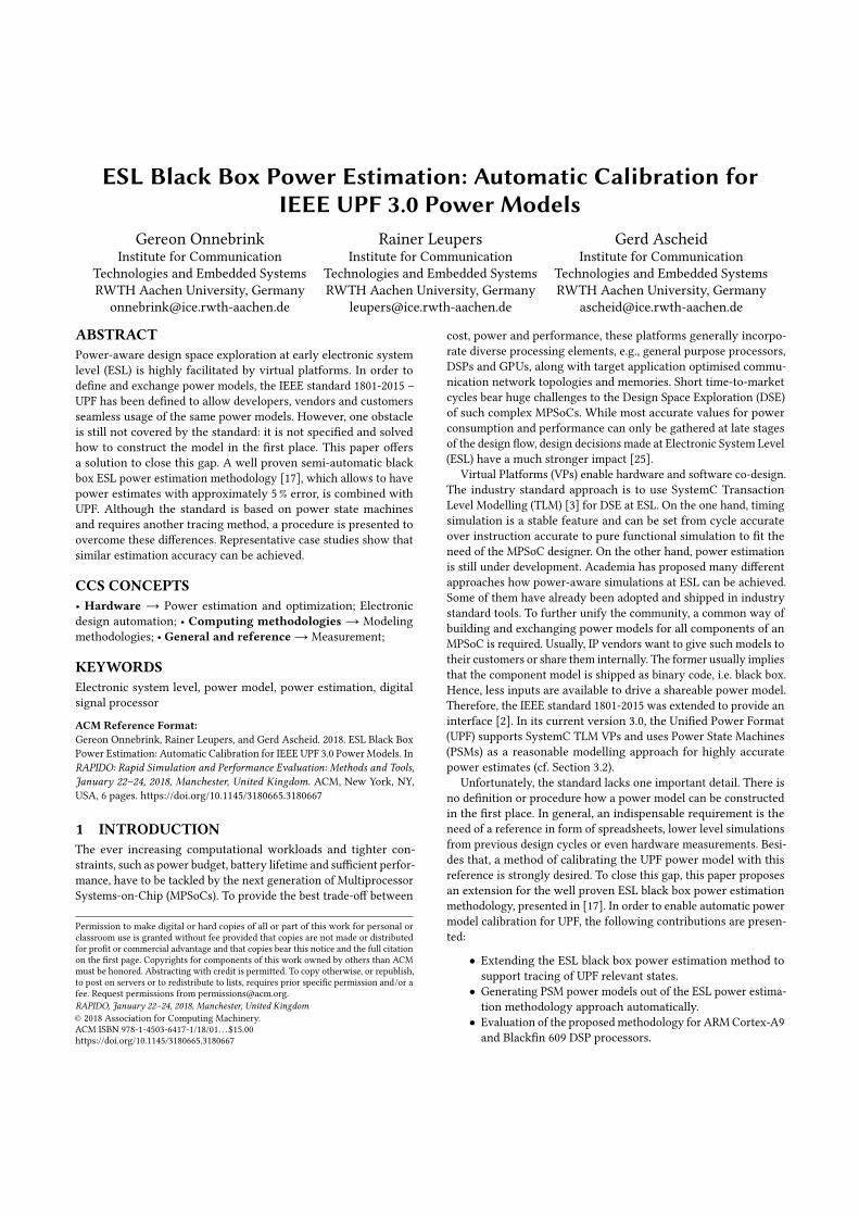
Pest = S · a = (1 s2 f · s3

) · ©­«afi1afi2afd3

ª®¬

afi1

afi2 f · afd3

0 0

s2,t = 0s2,t = 1 s3,t = 0s3,t = 1

Figure 1: Simplified example of a linear power model andthe corresponding PSMs

3 POWER ESTIMATION METHODOLOGYThe ESL power estimation methodology proposed in [17, 18] is thekey element for semi-automatic calibration of UPF power models.The concepts are first presented in [18] and modified to supportblack box power estimation [17]. Both are briefly summarised be-low. After that, an introduction to UPF is given, together with theapproach of generating PSMs out of the linear power model.

3.1 Linear Power ModelThe CMOS hardware power model is composed of two parts, theconstant leakage power and the dynamic power, which is depen-dent on short circuit and switching activity. The dynamic actionsperformed by the CMOS chip are driven by control signals initiatedby the application. Thus, tracing these control signals is enough toestimate the dynamic power.

Let there be N − 1 control signal traces, called ESL traces, eachrepresented by a column vector si ∈ RT , recorded over T samplingperiods of the length tsamp. To model the constant leakage power,the first trace is set to 1, i.e. s1 = 1. Combining all traces results inthe compact representation of the matrix S ∈ RT×N . Assuming alinear relation between the traces and the power consumption, theestimate can be calculated as shown in Equation 1, where a ∈ RNdenotes the so-called power model factors.

Pest = S · a (1)

Originally, this power estimation methodology supports onlyfixed frequency simulations. But in modern MPSoCs, DynamicVoltage and Frequency Scaling (DVFS) is a common approach toprovide a trade-off between power and performance. With a modi-fication, it is possible to build frequency aware power models byadding the current frequency in Equation 1 [17]. With this, explicitinformation about the frequency is added to the implicit one storedin each ESL trace.

P′est = S′ · a′ = (S f · S) · (afiafd

)(2)

where afi, afd ∈ RN denote the frequency independent and frequencydependent power model factors, respectively. An example linearpower model can be seen in the upper part of Figure 1.

ESL Black Box Power Estimation for IEEE UPF 3.0 Power Models RAPIDO, January 22–24, 2018, Manchester, United Kingdom

ARMCortex-A9

ARMCortex-A9

I-Cache32 kB

D-Cache32 kB

D-Cache32 kB

I-Cache32 kB

L2 Cache1MB

DRAM1GBUARTSpinlock

MemorySynchro-nisation

Coherency Bus

Simple Bus

Simple Bus

interrupts

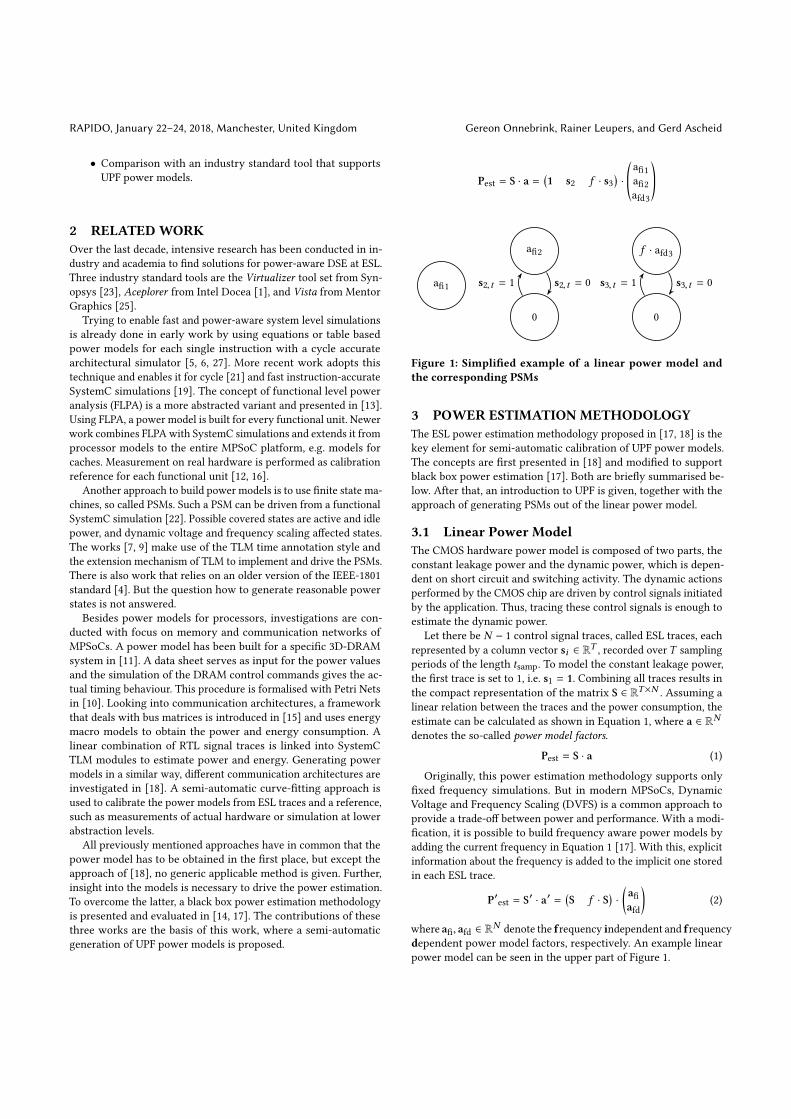
Figure 2: Virtual platform for the OMAP4460 ARM Cortex-A9 subsystem on the PandaBoard

3.2 IEEE 1801-2015 – UPFThe IEEE standard 1801-2015 [2], also known as UPF is the thirdrefinement and supports as new feature ESL power modelling andanalysis in virtual prototyping applications. Due to its history ofproviding an HDL-independent way of specifying power at earlystages in the design process, such as register transfer level, UPF isbasically an extension of the scripting language Tcl, and a collectionof directives of how to use the specified commands.

The power modelling concept is based on finite state machines,in this context also known as PSMs. Each state has a specific powervalue, either constant or computed by an equation which can bedependent to other input values, e.g. the current frequency. Transi-tions from one state to another are triggered by various inputs, suchas logic signal switches, timer events or SystemC TLM transactionevents. The latter forms the basis in this work to apply the blackbox constraint. As no internals can be observed in closed-sourcecomponents, only the inter module communication is available. Theprevious works [14, 17] and Section 5.1 show that TLM transacti-ons are sufficient for accurate power modelling. To represent thistransition mechanism, the trace matrix stores just the informationif a triggering event happened at a certain time, i.e. S ∈ {0, 1}T ′×N .T ′ is the number of sampling periods t ′samp, which is the shortesttime interval between two events.

Further, UPF can be used to partition a design into power dom-ains. Each domain has its own PSM and input trigger set. The sumover all domains determines the power consumption of the entireMPSoC. This not only reduces the complexity of a PSM, but alsoeases the transformation from the linear model approach to UPF.

3.3 Calibration of UPF PSMsFor the semi-automatic calibration of UPF PSMs, the linear powermodel of the estimation methodology presented in [17, 18] is used

Blackfin609 DSP

Blackfin609 DSP

D-Cache32 kB

I-Cache16 kB

D-Cache32 kB

I-Cache16 kB

L2 SRAM256KB

DRAM128MBUARTSpinlock

MemorySynchro-nisation

Simple Bus

interrupts

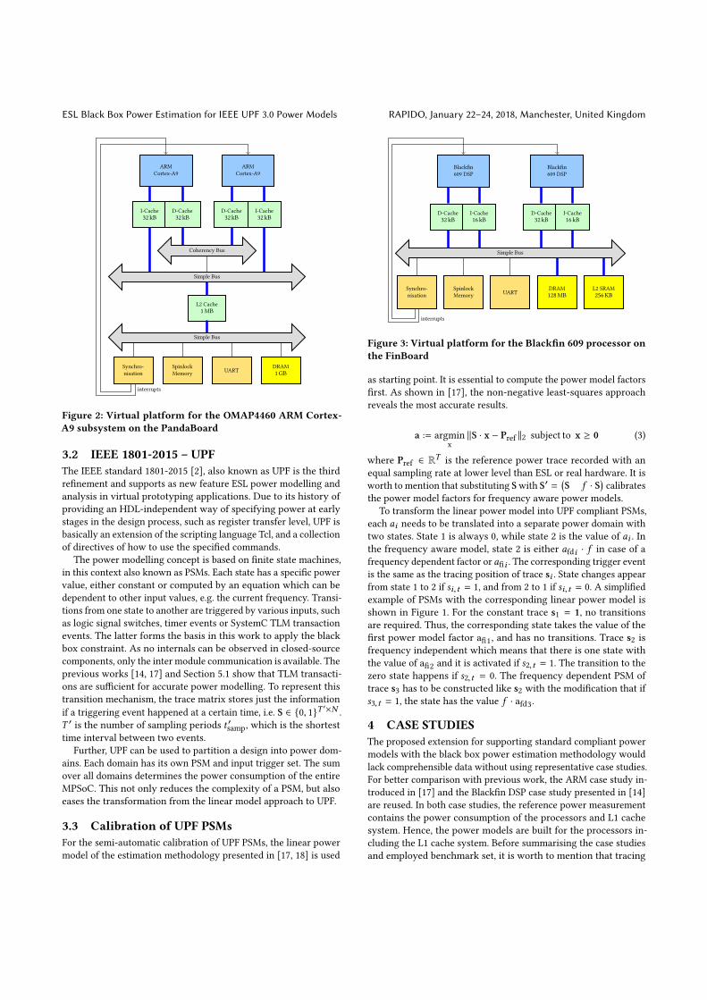
Figure 3: Virtual platform for the Blackfin 609 processor onthe FinBoard

as starting point. It is essential to compute the power model factorsfirst. As shown in [17], the non-negative least-squares approachreveals the most accurate results.

a := argminx

∥S · x − Pref ∥2 subject to x ≥ 0 (3)

where Pref ∈ RT is the reference power trace recorded with anequal sampling rate at lower level than ESL or real hardware. It isworth to mention that substituting Swith S′ =

(S f · S) calibrates

the power model factors for frequency aware power models.To transform the linear power model into UPF compliant PSMs,

each ai needs to be translated into a separate power domain withtwo states. State 1 is always 0, while state 2 is the value of ai . Inthe frequency aware model, state 2 is either afdi · f in case of afrequency dependent factor or afii . The corresponding trigger eventis the same as the tracing position of trace si . State changes appearfrom state 1 to 2 if si,t = 1, and from 2 to 1 if si,t = 0. A simplifiedexample of PSMs with the corresponding linear power model isshown in Figure 1. For the constant trace s1 = 1, no transitionsare required. Thus, the corresponding state takes the value of thefirst power model factor afi1, and has no transitions. Trace s2 isfrequency independent which means that there is one state withthe value of afi2 and it is activated if s2,t = 1. The transition to thezero state happens if s2,t = 0. The frequency dependent PSM oftrace s3 has to be constructed like s2 with the modification that ifs3,t = 1, the state has the value f · afd3.

4 CASE STUDIESThe proposed extension for supporting standard compliant powermodels with the black box power estimation methodology wouldlack comprehensible data without using representative case studies.For better comparison with previous work, the ARM case study in-troduced in [17] and the Blackfin DSP case study presented in [14]are reused. In both case studies, the reference power measurementcontains the power consumption of the processors and L1 cachesystem. Hence, the power models are built for the processors in-cluding the L1 cache system. Before summarising the case studiesand employed benchmark set, it is worth to mention that tracing

RAPIDO, January 22–24, 2018, Manchester, United Kingdom Gereon Onnebrink, Rainer Leupers, and Gerd Ascheid

has been adapted. In the previous work, counters are used for theso called TLM trace. This means, after every tsamp read and writecounters are stored and then reset to zero. This work introduces theTLM event trace, as UPF reacts on TLM transaction events. Hence,the trace stores every write and read occurrence of a TLM tran-saction, which can happen every t ′samp and is the shortest delaypossible in the VP, i.e., the time the shortest event lasts. This resultsin t ′samp ≪ tsamp. To keep the size of the traces reasonable, there isan averaging step added after tsamp. Consequently, the percentageof how often and long a TLM event happened during tsamp is stored.

Further abstraction similar to the introduced activity trace in [17]is still possible. Instead of using TLM triggering events, a plainSystemC signal is used to indicate whether a processor is activeor idle. Thus, the activity trace is set to one, if the core is running.Otherwise, the trace stores zero.

4.1 ARM Case StudyThe reference system for the ARM case study is the dual-core ARMsubsystem of the OMAP4460 SoC from the PandaBoard. The VPis composed around an instruction accurate ARM Cortex-A9 pro-cessor model from OVP. For this work, the instruction accuratestandalone simulator contained in the gdb-utils and encapsulated ina SystemC wrapper replaces the OVP processor model. Besides theARM, the entire memory hierarchy is assembled using an in-housevirtual component model library, i.e. L1 data cache with the im-plementation of the coherency mechanism, L2 caches, DRAM andbuses are present in the VP. All connections aremodelled using TLMblocking transactions, as this is sufficient for instruction accurateprocessor models. Average timing errors of 9 % are reported [17].Figure 2 illustrates the VP. The peripherals synchronisation andspinlock memory are used to implement and enable multi-threadedapplications. The locations of TLM event tracing are indicated bythick blue lines.

4.2 Blackfin Case StudyAs reference for the Blackfin case study, the dual core Blackfin 609DSP from the FinBoard is taken. The instruction accurate proces-sor model from gdb-utils is wrapped into SystemC context andused in the VP. From the same in-house virtual component modellibrary, the memory hierarchy is built, i.e. L1 caches, L2 SRAM,DRAM and buses. TLM blocking transactions are used to modelthe inter-component communication. The timing error of the VP ison average 6 % [14]. In Figure 3, the locations of TLM event tracingindicated by thick blue lines can be seen. As for the ARM case study,multi-threaded applications are enabled and executed using theperipherals synchronisation and spinlock memory.

4.3 BenchmarksThe benchmarks are executed without an operating system anddirectly run as bare-metal code. A representative benchmark sethas been chosen to stress and verify the methodology and revealrepresentative results. In-house benchmarks in addition to well-established standard benchmarks are used.

The standard benchmark selection contains: Dhrystone [26],LTE uplink receiver PHY benchmark [20] (abbreviated lte-bench),telecomm package of MiBench [8] (mib/t), StreamIt [24] (stit)

0 1 2 3 4 5

0.22

0.24

0.26

time (s)

power

(W)

reference (hardware measurement)estimate using Synopsys Virtualizer

estimate using BBPEM

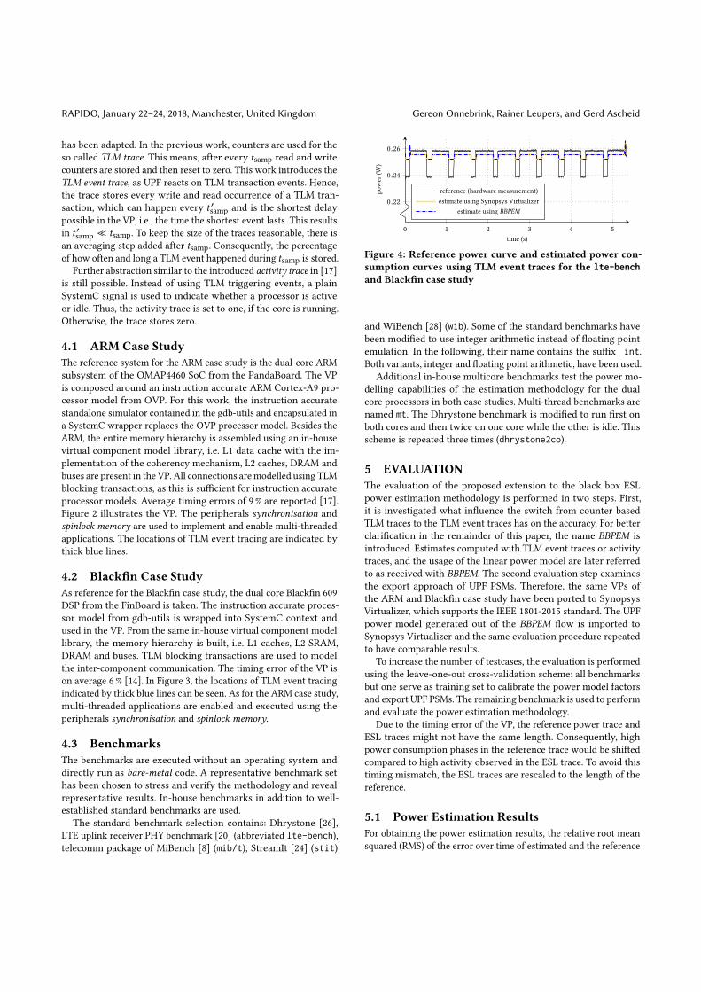
Figure 4: Reference power curve and estimated power con-sumption curves using TLM event traces for the lte-benchand Blackfin case study

and WiBench [28] (wib). Some of the standard benchmarks havebeen modified to use integer arithmetic instead of floating pointemulation. In the following, their name contains the suffix _int.Both variants, integer and floating point arithmetic, have been used.

Additional in-house multicore benchmarks test the power mo-delling capabilities of the estimation methodology for the dualcore processors in both case studies. Multi-thread benchmarks arenamed mt. The Dhrystone benchmark is modified to run first onboth cores and then twice on one core while the other is idle. Thisscheme is repeated three times (dhrystone2co).

5 EVALUATIONThe evaluation of the proposed extension to the black box ESLpower estimation methodology is performed in two steps. First,it is investigated what influence the switch from counter basedTLM traces to the TLM event traces has on the accuracy. For betterclarification in the remainder of this paper, the name BBPEM isintroduced. Estimates computed with TLM event traces or activitytraces, and the usage of the linear power model are later referredto as received with BBPEM. The second evaluation step examinesthe export approach of UPF PSMs. Therefore, the same VPs ofthe ARM and Blackfin case study have been ported to SynopsysVirtualizer, which supports the IEEE 1801-2015 standard. The UPFpower model generated out of the BBPEM flow is imported toSynopsys Virtualizer and the same evaluation procedure repeatedto have comparable results.

To increase the number of testcases, the evaluation is performedusing the leave-one-out cross-validation scheme: all benchmarksbut one serve as training set to calibrate the power model factorsand export UPF PSMs. The remaining benchmark is used to performand evaluate the power estimation methodology.

Due to the timing error of the VP, the reference power trace andESL traces might not have the same length. Consequently, highpower consumption phases in the reference trace would be shiftedcompared to high activity observed in the ESL trace. To avoid thistiming mismatch, the ESL traces are rescaled to the length of thereference.

5.1 Power Estimation ResultsFor obtaining the power estimation results, the relative root meansquared (RMS) of the error over time of estimated and the reference

ESL Black Box Power Estimation for IEEE UPF 3.0 Power Models RAPIDO, January 22–24, 2018, Manchester, United Kingdom

dhrystone

dhrystone2co

lte-bench

lte-bench

_int

mib/t/adpcm

mib/t/CR

C32

mib/t/FFT

mib/t/gsm

mt/audio_filter

mt/mandelbrot

mt/matm

ult

mt/sobel_co

arse

stit/bitonic-sortstit/fft

stit/fft_int

stit/filterban

kstit/fm

stit/matm

ul-blk

stit/matm

ul-blk_int

stit/matrixm

ult

stit/matrixm

ult_int

wib/C

hannel

wib/Equalizer

wib/LTESys

wib/M

odDemod

wib/RateMatcher

wib/SCFDM

A

wib/ScrambDescramb

wib/SubCarrierM

apDemap

wib/TransformPreDec

wib/Turbo

10

20

relativ

eRM

Spo

wer

estim

ationerror(%)

TLM event traces - ARM activity traces - ARM TLM event traces - Blackfin activity traces - Blackfin

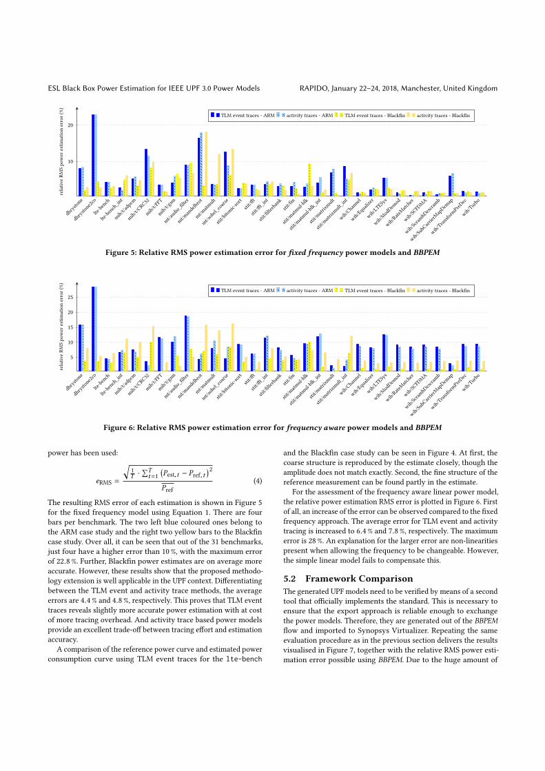
Figure 5: Relative RMS power estimation error for fixed frequency power models and BBPEM

dhrystone

dhrystone2co

lte-bench

lte-bench

_int

mib/t/adpcm

mib/t/CR

C32

mib/t/FFT

mib/t/gsm

mt/audio_filter

mt/mandelbrot

mt/matm

ult

mt/sobel_co

arse

stit/bitonic-sortstit/fft

stit/fft_int

stit/filterban

kstit/fm

stit/matm

ul-blk

stit/matm

ul-blk_int

stit/matrixm

ult

stit/matrixm

ult_int

wib/C

hannel

wib/Equalizer

wib/LTESys

wib/M

odDemod

wib/RateMatcher

wib/SCFDM

A

wib/ScrambDescramb

wib/SubCarrierM

apDemap

wib/TransformPreDec

wib/Turbo

5

10

15

20

25

relativ

eRM

Spo

wer

estim

ationerror(%)

TLM event traces - ARM activity traces - ARM TLM event traces - Blackfin activity traces - Blackfin

Figure 6: Relative RMS power estimation error for frequency aware power models and BBPEM

power has been used:

eRMS =

√1T ·∑T

t=1(Pest,t − Pref,t

)2Pref

(4)

The resulting RMS error of each estimation is shown in Figure 5for the fixed frequency model using Equation 1. There are fourbars per benchmark. The two left blue coloured ones belong tothe ARM case study and the right two yellow bars to the Blackfincase study. Over all, it can be seen that out of the 31 benchmarks,just four have a higher error than 10 %, with the maximum errorof 22.8 %. Further, Blackfin power estimates are on average moreaccurate. However, these results show that the proposed methodo-logy extension is well applicable in the UPF context. Differentiatingbetween the TLM event and activity trace methods, the averageerrors are 4.4 % and 4.8 %, respectively. This proves that TLM eventtraces reveals slightly more accurate power estimation with at costof more tracing overhead. And activity trace based power modelsprovide an excellent trade-off between tracing effort and estimationaccuracy.

A comparison of the reference power curve and estimated powerconsumption curve using TLM event traces for the lte-bench

and the Blackfin case study can be seen in Figure 4. At first, thecoarse structure is reproduced by the estimate closely, though theamplitude does not match exactly. Second, the fine structure of thereference measurement can be found partly in the estimate.

For the assessment of the frequency aware linear power model,the relative power estimation RMS error is plotted in Figure 6. Firstof all, an increase of the error can be observed compared to the fixedfrequency approach. The average error for TLM event and activitytracing is increased to 6.4 % and 7.8 %, respectively. The maximumerror is 28 %. An explanation for the larger error are non-linearitiespresent when allowing the frequency to be changeable. However,the simple linear model fails to compensate this.

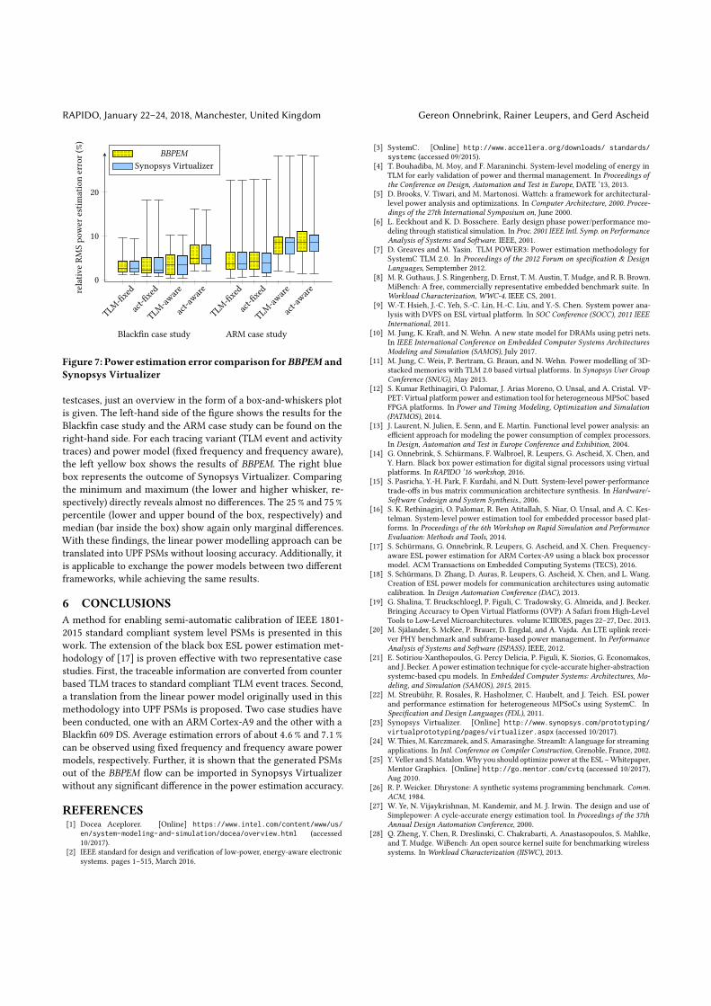
5.2 Framework ComparisonThe generated UPF models need to be verified by means of a secondtool that officially implements the standard. This is necessary toensure that the export approach is reliable enough to exchangethe power models. Therefore, they are generated out of the BBPEMflow and imported to Synopsys Virtualizer. Repeating the sameevaluation procedure as in the previous section delivers the resultsvisualised in Figure 7, together with the relative RMS power esti-mation error possible using BBPEM. Due to the huge amount of

RAPIDO, January 22–24, 2018, Manchester, United Kingdom Gereon Onnebrink, Rainer Leupers, and Gerd Ascheid

TLM-fixed

act-fixed

TLM-aware

act-aw

are

TLM-fixed

act-fixed

TLM-aware

act-aw

are0

10

20

relativ

eRM

Spo

wer

estim

ationerror(%)

BBPEMSynopsys Virtualizer

Blackfin case study ARM case study

Figure 7: Power estimation error comparison forBBPEM andSynopsys Virtualizer

testcases, just an overview in the form of a box-and-whiskers plotis given. The left-hand side of the figure shows the results for theBlackfin case study and the ARM case study can be found on theright-hand side. For each tracing variant (TLM event and activitytraces) and power model (fixed frequency and frequency aware),the left yellow box shows the results of BBPEM. The right bluebox represents the outcome of Synopsys Virtualizer. Comparingthe minimum and maximum (the lower and higher whisker, re-spectively) directly reveals almost no differences. The 25 % and 75 %percentile (lower and upper bound of the box, respectively) andmedian (bar inside the box) show again only marginal differences.With these findings, the linear power modelling approach can betranslated into UPF PSMs without loosing accuracy. Additionally, itis applicable to exchange the power models between two differentframeworks, while achieving the same results.

6 CONCLUSIONSA method for enabling semi-automatic calibration of IEEE 1801-2015 standard compliant system level PSMs is presented in thiswork. The extension of the black box ESL power estimation met-hodology of [17] is proven effective with two representative casestudies. First, the traceable information are converted from counterbased TLM traces to standard compliant TLM event traces. Second,a translation from the linear power model originally used in thismethodology into UPF PSMs is proposed. Two case studies havebeen conducted, one with an ARM Cortex-A9 and the other with aBlackfin 609 DS. Average estimation errors of about 4.6 % and 7.1 %can be observed using fixed frequency and frequency aware powermodels, respectively. Further, it is shown that the generated PSMsout of the BBPEM flow can be imported in Synopsys Virtualizerwithout any significant difference in the power estimation accuracy.

REFERENCES[1] Docea Aceplorer. [Online] https://www.intel.com/content/www/us/

en/system-modeling-and-simulation/docea/overview.html (accessed10/2017).

[2] IEEE standard for design and verification of low-power, energy-aware electronicsystems. pages 1–515, March 2016.

[3] SystemC. [Online] http://www.accellera.org/downloads/ standards/systemc (accessed 09/2015).

[4] T. Bouhadiba, M. Moy, and F. Maraninchi. System-level modeling of energy inTLM for early validation of power and thermal management. In Proceedings ofthe Conference on Design, Automation and Test in Europe, DATE ’13, 2013.

[5] D. Brooks, V. Tiwari, and M. Martonosi. Wattch: a framework for architectural-level power analysis and optimizations. In Computer Architecture, 2000. Procee-dings of the 27th International Symposium on, June 2000.

[6] L. Eeckhout and K. D. Bosschere. Early design phase power/performance mo-deling through statistical simulation. In Proc. 2001 IEEE Intl. Symp. on PerformanceAnalysis of Systems and Software. IEEE, 2001.

[7] D. Greaves and M. Yasin. TLM POWER3: Power estimation methodology forSystemC TLM 2.0. In Proceedings of the 2012 Forum on specification & DesignLanguages, Semptember 2012.

[8] M. R. Guthaus, J. S. Ringenberg, D. Ernst, T. M. Austin, T. Mudge, and R. B. Brown.MiBench: A free, commercially representative embedded benchmark suite. InWorkload Characterization, WWC-4. IEEE CS, 2001.

[9] W.-T. Hsieh, J.-C. Yeh, S.-C. Lin, H.-C. Liu, and Y.-S. Chen. System power ana-lysis with DVFS on ESL virtual platform. In SOC Conference (SOCC), 2011 IEEEInternational, 2011.

[10] M. Jung, K. Kraft, and N. Wehn. A new state model for DRAMs using petri nets.In IEEE International Conference on Embedded Computer Systems ArchitecturesModeling and Simulation (SAMOS), July 2017.

[11] M. Jung, C. Weis, P. Bertram, G. Braun, and N. Wehn. Power modelling of 3D-stacked memories with TLM 2.0 based virtual platforms. In Synopsys User GroupConference (SNUG), May 2013.

[12] S. Kumar Rethinagiri, O. Palomar, J. Arias Moreno, O. Unsal, and A. Cristal. VP-PET: Virtual platform power and estimation tool for heterogeneous MPSoC basedFPGA platforms. In Power and Timing Modeling, Optimization and Simulation(PATMOS), 2014.

[13] J. Laurent, N. Julien, E. Senn, and E. Martin. Functional level power analysis: anefficient approach for modeling the power consumption of complex processors.In Design, Automation and Test in Europe Conference and Exhibition, 2004.

[14] G. Onnebrink, S. Schürmans, F. Walbroel, R. Leupers, G. Ascheid, X. Chen, andY. Harn. Black box power estimation for digital signal processors using virtualplatforms. In RAPIDO ’16 workshop, 2016.

[15] S. Pasricha, Y.-H. Park, F. Kurdahi, and N. Dutt. System-level power-performancetrade-offs in bus matrix communication architecture synthesis. In Hardware/-Software Codesign and System Synthesis., 2006.

[16] S. K. Rethinagiri, O. Palomar, R. Ben Atitallah, S. Niar, O. Unsal, and A. C. Kes-telman. System-level power estimation tool for embedded processor based plat-forms. In Proceedings of the 6th Workshop on Rapid Simulation and PerformanceEvaluation: Methods and Tools, 2014.

[17] S. Schürmans, G. Onnebrink, R. Leupers, G. Ascheid, and X. Chen. Frequency-aware ESL power estimation for ARM Cortex-A9 using a black box processormodel. ACM Transactions on Embedded Computing Systems (TECS), 2016.

[18] S. Schürmans, D. Zhang, D. Auras, R. Leupers, G. Ascheid, X. Chen, and L. Wang.Creation of ESL power models for communication architectures using automaticcalibration. In Design Automation Conference (DAC), 2013.

[19] G. Shalina, T. Bruckschloegl, P. Figuli, C. Tradowsky, G. Almeida, and J. Becker.Bringing Accuracy to Open Virtual Platforms (OVP): A Safari from High-LevelTools to Low-Level Microarchitectures. volume ICIIIOES, pages 22–27, Dec. 2013.

[20] M. Själander, S. McKee, P. Brauer, D. Engdal, and A. Vajda. An LTE uplink recei-ver PHY benchmark and subframe-based power management. In PerformanceAnalysis of Systems and Software (ISPASS). IEEE, 2012.

[21] E. Sotiriou-Xanthopoulos, G. Percy Delicia, P. Figuli, K. Siozios, G. Economakos,and J. Becker. A power estimation technique for cycle-accurate higher-abstractionsystemc-based cpu models. In Embedded Computer Systems: Architectures, Mo-deling, and Simulation (SAMOS), 2015, 2015.

[22] M. Streubühr, R. Rosales, R. Hasholzner, C. Haubelt, and J. Teich. ESL powerand performance estimation for heterogeneous MPSoCs using SystemC. InSpecification and Design Languages (FDL), 2011.

[23] Synopsys Virtualizer. [Online] http://www.synopsys.com/prototyping/virtualprototyping/pages/virtualizer.aspx (accessed 10/2017).

[24] W. Thies, M. Karczmarek, and S. Amarasinghe. StreamIt: A language for streamingapplications. In Intl. Conference on Compiler Construction, Grenoble, France, 2002.

[25] Y. Veller and S.Matalon. Why you should optimize power at the ESL –Whitepaper,Mentor Graphics. [Online] http://go.mentor.com/cvtq (accessed 10/2017),Aug 2010.

[26] R. P. Weicker. Dhrystone: A synthetic systems programming benchmark. Comm.ACM, 1984.

[27] W. Ye, N. Vijaykrishnan, M. Kandemir, and M. J. Irwin. The design and use ofSimplepower: A cycle-accurate energy estimation tool. In Proceedings of the 37thAnnual Design Automation Conference, 2000.

[28] Q. Zheng, Y. Chen, R. Dreslinski, C. Chakrabarti, A. Anastasopoulos, S. Mahlke,and T. Mudge. WiBench: An open source kernel suite for benchmarking wirelesssystems. In Workload Characterization (IISWC), 2013.

XII

Beyond Time-TriggeredCo-simulation of Cyber-PhysicalSystems for Performance andAccuracy Improvements

XIII

Beyond Time-Triggered Co-simulation of Cyber-PhysicalSystems for Performance and Accuracy Improvements.

Giovanni LiboniUniversite Cote d’Azur, InriaSophia Antipolis, Francegiovanni.liboni@inria.fr

Julien DeantoniUniversite Cote d’Azur,

CNRS, I3S, InriaSophia Antipolis, France

deantoni@polytech.unice.fr

Antonio PortaluriEDALab SrlVerona, Italy

antonio.portulari@edalab.it

Davide QuagliaDepartment of Computer Science,

University of Verona, Italydavide.quaglia@univr.it

Robert de SimoneUniversite Cote d’Azur, InriaSophia Antipolis, Francerobert.de_simone@inria.fr

ABSTRACTCyber-Physical Systems consist of cyber components con-trolling physical entities. Their development involves dif-ferent engineering disciplines, that use different models,written in languages with different semantics. A coupledsimulation of these models is of prime importance to rapidlyunderstand the emerging system behavior. The coupling ofthe simulations is realized by a coordinator that conveysdata and ensures time consistency between the differentmodels/simulators. Existing coordinators are usually timetriggered. In this paper we show that time-triggered co-ordinators may introduce poor performance and accuracy(both temporal and functional) when used to co-simulatecyber-physical models. Therefore, we propose a new coor-dinator mixing time- and event-triggered mechanisms. Wevalidated the approach in the context of the FMI standard forco-simulation. To make possible the writing of the new coor-dinators, we implemented backward compatible extensionsto the FMI API. Also, we implemented a new FMI exporterin an industrial tool.

KEYWORDSFMI, Functional Mock-up Interface, event-driven simulation

ACM Reference Format:Giovanni Liboni, JulienDeantoni, Antonio Portaluri, DavideQuaglia,and Robert de Simone. 2018. Beyond Time-Triggered Co-simulationof Cyber-Physical Systems for Performance and Accuracy Improve-ments.. In RAPIDO: Rapid Simulation and Performance Evaluation:

Publication rights licensed to ACM. ACM acknowledges that this contribu-tion was authored or co-authored by an employee, contractor or affiliateof a national government. As such, the Government retains a nonexclusive,royalty-free right to publish or reproduce this article, or to allow others to doso, for Government purposes only.RAPIDO, January 22–24, 2018, Manchester, United Kingdom© 2018 Copyright held by the owner/author(s). Publication rights licensed toAssociation for Computing Machinery.ACM ISBN 978-1-4503-6417-1/18/01. . . $15.00https://doi.org/10.1145/3180665.3180668

Methods and Tools, January 22–24, 2018, Manchester, United King-dom. ACM, New York, NY, USA, Article x, 8 pages. https://doi.org/10.1145/3180665.3180668

1 INTRODUCTIONIn Cyber-Physical Systems (CPS) digital systems (eventuallydistributed) are in charge of controlling physical entitiesin the environment, e.g., mechanical, chemical or thermalmechanisms. Modeling and simulation are traditional tech-niques to support design but in CPS’s there is a mix of dif-ferent engineering disciplines [18] each of them using adomain-specific modeling language with its syntax and se-mantics. The simulation of such systems should addressa mix of heterogeneous models whose coupling make thebehavior of the system under modeling emerging [8]. Toensure a fast time to market, it is important to understandsuch emerging behavior early in the development process.

In this context, co-simulation is a key enabler. It consistsin the coordinated simulation of different parts of the CPS byusing specific solvers/interpreters for the different modelingapproaches. The “coordinator” among the simulators mustensure the timely exchange of data between the differentsolvers/interpreters according to a so-called “master algo-rithm”. The development of such coordinator usually relieson the graph representing the sharing of data between thedifferent models [2, 4, 5, 24]. It also depends on the natureof the interaction between the different models [10].

For instance, when the data shared between two mod-els have a causal relationship (e.g., a producer-consumerrelationship) then the coordinator must ensure that it isrespected during the co-simulation. In literature, there arecoordination languages to define a partial order between theexecution of the models [22].

This coordinator is crucial for the correctness and ef-ficiency of the co-simulation so that many master algo-rithms have been proposed [1, 2, 4, 5, 21, 23, 24, 27, 28].It is worth noticing that all the proposed algorithms aretime triggered, i.e., model execution is forced at predefined

RAPIDO, January 22–24, 2018, Manchester, United Kingdom G. Liboni et al.

time-steps. This is a surprising fact since from the 90’s workabout coordination languages and architecture descriptionlanguages (ADLs) proposed more sophisticated techniquesfor the correct and efficient coordination among softwarecomponents [13, 19, 22].

In this paper, we highlight the loss of efficiency and ac-curacy introduced by the use of pure time-triggered coordi-nators by presenting minimal illustrating examples. Then,we leverage work done in the community to introduce newmaster algorithms, especially relevant for CPS since theymix event and time trigger mechanisms. Finally, we presentexperimental results for co-simulation based on the FMI [20]industrial standard where VHDL digital models are coordi-nated with Modelica physical models. To enable the writingof new coordination algorithm, we extended the FMI stan-dard in a backward compatible way.

2 BACKGROUND ON TIME-TRIGGEREDCOORDINATORS

The most common coordinator runs each model for a step(i.e., a fixed period of time), collects the outputs from allsubsystems and conveys outputs to the inputs of themodel(s)of interest. Finally, it continues the (co-)simulation for therequired simulation time 1.

In a model, when a discontinuity appears during the sim-ulation of a step, it may reject the step or not depending onits implementation. If the step is rejected, the model returnsthe discontinuity time to the coordinator and all the modelsthat already simulated the current step need to be rolledback to their previously saved state. Then they are askedto simulate until the time of the discontinuity, values areexchanged and the simulation continues in a time-drivenfashion. If the step is not rejected, then the exact time of thediscontinuity is unknown; it occurred during the step. Notethat implementation of the rollback procedures is costly, notalways implemented, and according to [9], it may be difficultto achieve in practice, especially for cyber models.

To understand how to write a coordinator, it is importantto understand that cyber and physical models are funda-mentally different in the way they are executed (i.e., theyfollow a different Model of Computation). These differenceshave already been identified and studied in the context ofco-simulation [4, 5, 26]. However, the goal of these studieswas not to propose an appropriate coordinator but rather toproposed functional and temporal adaptation consideringthese differences.

Physical models are usually defined by equations (e.g.,ODE or DAE) which can be solved at any points in time and anumerical approach is used to choose the most appropriateddiscretization. Usually, in such physical models, smaller thediscretization step is, better the accuracy is.

1many variants of this simple abstraction are available in the literature [1, 2,4, 5, 21, 23, 24, 27, 28] but the main idea is the same.

Cyber models are based on the notion of, possibly parallel,sequences of instructions and data are read or written at spe-cific points in time which depend on the program structureand are not necessarily periodic. So it is not possible to use anumerical method to compute an appropriate constant stepsize. In the context of time-triggered simulation, each datatransfer can then be seen as a discontinuity and may involvestep rejection with state saving/restoring thus inducing apossible large overhead at runtime [9]. When step rejectionis not used it implies accuracy problems (see Section 3).

In summary, the designer can either use step rejection(when implemented) or reduce the co-simulation step; inboth cases there is a loss in simulation speed [6]. If the co-simulation step is increased, simulation accuracy is reduced.Therefore, a time-triggered coordinator in the presence of cy-ber model(s) forces to have a trade-off between performanceand accuracy.

3 MIX EVENT- AND TIME-TRIGGEREDCOORDINATOR FOR CPS

3.1 OverviewWewant to enable the use of cybermodels for the co-simulationof cyber-physical systems. Based on previous experimentson synchronous languages [3] and the coordination of het-erogeneous cyber models [7, 16, 17] we believe that coor-dinators could be more accurate and efficient if we allowevent-driven communication between the coordinator andthe models under execution. Our goal is twice. On the onehand, we want to improve the efficiency of the simulationby 1) avoiding roll back as much as possible and 2) reducingthe communication between a model under simulation andthe coordinator. On the other hand, we want to improve theaccuracy (both temporal and functional) by letting a modelsimulate until an event of interest occurs.

This is a well-known mechanism in distributed systemswhere unnecessary communications are avoided and wherelogical clocks are used to synchronize the systems [11, 15].This means that the coordinator must be tuned, accordingto both the data sharing topology and their properties toavoid as much as possible the unnecessary synchronizationsbetween the model simulations, letting them simulate untila communication is required.

In the next subsections, we describe three examples thathighlight a particular problemwithin the current time-triggeredcoordinators. We also propose a coordinator to solve theproblem2.

2All the experiments presented in this paper, the results and the implementa-tions are provided here https://project.inria.fr/fidel/rapido2018/

Beyond Time-Triggered Co-simulation of CPS RAPIDO, January 22–24, 2018, Manchester, United Kingdom

3.2 Coordination of a cyber model withdiscrete output

The first example shows limitations of the time-triggeredcoordination for a cyber model with a discrete output.

Let us consider the cyber model of a wheel encoder driver(C1), producing a discrete signal v1. A wheel encoder is asensor that allows tracking the number of wheel rotations.More precisely, the output of the driver switches from 0 to1 or conversely each time a 1/32 of revolution of a wheelis done. Signal v1 is consumed by another model (P1) (seeFigure 1), which computes the actual speed of the wheelaccording to the time spent between two successive switchesof v1. Consequently, v1 is assigned only at specific points intime, depending on the speed of the wheel. This assignmentcreates a discontinuity, which is neither a rare event orsymptomatic of a specific phenomenon like in models ofphysical systems.

In order for the co-simulation to be correct, all data assign-ments should be seen by the coordinator and transferredto P1 at the right time. More generally, such discontinu-ity implies different problems: a temporal inaccuracy, i.e.,the changes in the output values are seen by the coordi-nator at wrong points in time; a functional inaccuracy, i.e.,the coordinator is missing some of the discontinuities; or aperformance problem, i.e., the roll back mechanism is usedintensively.

Figure 1: ModelC1 produces data v1 consumed by P1.

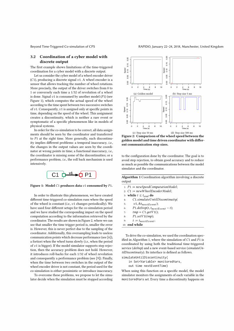
In order to illustrate this phenomenon, we have createddifferent time-triggered co-simulation runs where the speedof the wheel is constant (i.e., v1 changes periodically). Wehave used four different setups for the co-simulation periodand we have studied the corresponding impact on the speedcomputation according to the information retrieved by thecoordinator. The results are shown in Figure 2, where we cansee that smaller the time trigger period is, smaller the erroris. However, this is never perfect due to the sampling of thecoordinator. Additionally, this oversampling leads to uselesscommunication points which decrease performance (see [6]),a fortiori when the wheel turns slowly (i.e., when the periodof v1 is bigger). If the model simulator supports step rejec-tion, then the accuracy problem does not hold. However,it introduces roll-backs for each 1/32 of wheel revolutionand consequently a performance problem (see [9]). Finally,when the time between two switches in the output of thewheel encoder driver is not constant, the period used for theco-simulation is either pessimistic or introduce inaccuracy.

To overcome these problems, we propose to let the simu-lator decide when the simulation must be stopped according

(a) Golden model (b) Step size 5 ms

(c) Step size 50 ms (d) Step size 500 msFigure 2: Comparison of the wheel speed between thegoldenmodel and time driven coordinatorwith differ-ent communication step sizes.

to the configuration done by the coordinator. The goal is toavoid step rejection, to obtain good accuracy and to reduceas much as possible the communications between the modelsimulator and the coordinator.

Algorithm 1 Coordination algorithm involving a discreteoutput1: P1 := newSpeedComputationModel ;2: C1 := newWheelEncoderModel ;3: while t ≤ tend do4: C1.simulateUntilDiscontinuity(5: v1,&tnextEvent );6: P1.doStep(t , tnextEvent − t);7: tmp = C1.дetV 1();8: P1.setV 1(tmp);9: t := tnextEvent ;10: end while

To drive the co-simulation, we used the coordination spec-ified in Algorithm 1, where the simulation of C1 and P1 iscoordinated by using both the traditional time-triggeredservice (doStep) and a new event-based service (simulateUn-tilDiscontinuity). Its interface is defined as follows.simulateUntilDiscontinuity(

in Set<Variable> monitoredVars,out time nextEventTime)

When using this function on a specific model, the modelsimulator monitors the assignments of each variable in themonitoredVars set. Every time a discontinuity happens on

RAPIDO, January 22–24, 2018, Manchester, United Kingdom G. Liboni et al.

one of these variables, the function sets nextEventTimeto its current internal time and returns immediately. Thefunction takes two parameters:

• The monitoredVars input parameter is the list of vari-ables the model simulation has to monitor, lookingfor a discontinuity;

• The nextEventTime output parameter returns the in-ternal simulation time when a discontinuity occurred.

The main idea of the coordinator algorithm is that thecoordinator asks C1 to simulate until a discontinuity is de-tected on v1. When the function returns, the coordinatorknows 1) the exact time of the assignment and 2) that thisis the first assignment of interest that happened betweentime t and tnextEvent . Then the coordinator calls the doStepfunction on P1 (line 6) to simulate it until the time at whichthe discontinuity appeared inC1. Then, it retrieves the valuethat caused the discontinuity from C1 and set it to P1 (line7 and 8). By using this coordination algorithm, the numberof communication points is equal to the number of disconti-nuities in the cyber model (i.e., the smallest one to retrieveall the values of the variable) and the timestamps of thediscontinuities are precisely known. This simple coordina-tion provides no rollback, no overhead in the co-simulationexecution time and perfect temporal accuracy.

3.3 Coordination of a cyber model withinput(s)

As a second example, consider a cyber modelC1 that sensesthe environment (e.g., a room, a CPU) and computes thetemperature. Usually, in the actual implementation of suchsystem, the environment is sensed periodically. We considerhere that the environment that provides the temperatureevolution is modeled by a physical model P1whose output isread periodically byC1 (see Figure 3). In usual time-triggeredco-simulation, the co-simulation period is chosen so that thedata obtained by the physical model is fresh enough whenpropagated to the cyber model.

Figure 3: Model P1 produces data v1 consumed byC1.

There are three drawbacks here. First, the cyber modelis called several times to update its input even if this inputis not required to be read internally thus wasting simula-tion time. Second, the physical model is called several timesto compute fresh values that are actually not used by thecyber model. Third, there is no synchronization betweenthe actual reading of the input by the cyber model and itsupdate by the coordinator. This can lead to a temporal in-accuracy since the actual reading can occur at the end of asimulation step, i.e., without a fresh input. In this case, either

the designer considers that the freshness of the data is notimportant (but that can lead to wrong simulation results!) or the designer decreases the co-simulation period andconsequently decreases the performance.

As shown in the previous section, increasing the numberof communication points between models and coordinatorfor better accuracy decreases the overall performance andtherefore we aim at reducing the number of communicationpoints without reducing accuracy.

To solve this problem, we propose to enable the simula-tion of a model until the precise time when it is ready tointernally read on one of its inputs. It provides the coordina-tor with the time at which the read operation will be actuallydone. On the one hand it avoids unnecessary calls to thecyber model simulator; on the other hand, the coordinatorcan ask the physical model to compute the input data at theexact time it will be read by the cyber model (by calling thetraditional doStep method with the appropriate communi-cation step size). At the next call of the cyber model, it willread the input data that has been updated specifically for it.

Algorithm 2 describes the coordinator that implementssuch proposition. In this case, C1 is simulated first (line 4and 5). When it returns, P1 is simulated until the readingtime of C1 (line 6). Then the value retrieved from P1 is sentto C1 (line 7 and 8).

Algorithm 2 Co-simulation Master Algorithm read opera-tion1: P1 := newEnvFMU ;2: C1 := newSensorDriverFMU ;3: while t ≤ tend do4: C1.simulateUntilRead(5: v1,&tnextEvent );6: P1.doStep(t , tnextEvent − t);7: tmp = P1.дetV 1();8: C1.setV 1(tmp);9: t := tnextEvent ;10: end while

To create this coordination we used a new event-basedinterface named simulateUntilRead, defined as follows:simulateUntilRead(

in Set<Variable> inVars,out Time& nextEventTime)

It enables the simulation of a model until it is ready to do aread operation on one of the input variables in the inVarsset. The function takes two parameters:

• The inVars input parameter is a list of sensitive Vari-able for which the function should return before theircommunication;

• The nextEventTime output parameter provides theinternal simulator time just before the read occurs.

Beyond Time-Triggered Co-simulation of CPS RAPIDO, January 22–24, 2018, Manchester, United Kingdom

3.4 Conditional simulationSometimes, input values of a model internally participatein a conditional statement. Depending on the condition,different behaviors are chosen (e.g., by using a traditionalif statement). For instance, let us consider a simple counterC1 that increments a value v1 consumed by a model P1.Internally to P1, when v1 reaches a specific value, then P1changes its behavior. Usually, this is implemented in co-simulation by periodically providing the input value to themodel, which checks if the value reaches the condition ornot. To avoid previously presented drawbacks, a designercould use the coordinator presented in section 3.2 where theinput value is provided with a good temporal precision. Wego further here by defining a coordinator that asks a modelto simulate until a specific condition is reached on one of itsoutput variables. This avoids unnecessary communicationpoints between the model simulators and the coordinatorand consequently provides better performance.

The coordinator used in this case (Algorithm 3) is similarto Algorithm 1. However, during the setup phase, it retrievesthe predicates from P1 to construct the condition variablessent as a parameter of C1 simulation.

Algorithm 3 Coordination Algorithm with Predicate1: C1 := newEnvFMU ;2: P1 := newSensorFMU ;3: conds := P1.дetPredicates();4: condVars := setupVars(conds);5: while t ≤ tend do6: C1.simulateUntilCondition(7: condVars,&tnextEvent );8: ... (see Algorithm 1)9: end while

This coordinator uses a new event-based interface to han-dle conditional checks:simulateUntilCondition(

Set<CondVariable> outVars,Fmu2Time& nextEventTime)

CondVariable extends the Variable structurewith a Booleanpredicate. Using this interface, the model providing data issimulated and each time an assignment is done on one ofthe variables in outVars, then the predicate is evaluated.When a predicate is evaluated to True, then the functionreturns. This interface can have a positive effect on per-formance provided that more information about the modelinternal behavior are available with respect to traditionalco-simulation.

4 TOOL INTEGRATIONIn this section, we present the technical background used forthe experiments. We are going to present FMI, the industrial

co-simulation standard, and HIFSuite, a tool suite to performmodel manipulation.

4.1 FMI - Functional Mock-up InterfaceFMI is a tool-independent standard framework for co-simula-tion of dynamic models. The FMI standard is managed anddeveloped as a Modelica Association Project. FMI provides astandardized interface allowing different executable models(named FMU: Functional Mock-up Unit) to be controlledby an external software entity. The data exchange betweenmodels is restricted to communication points. Between twocommunication points (i.e., during a simulation step), themodels are solved independently by each FMU simulator.The coordination is implemented by the so-called MasterAlgorithm (MA). FMI standard regulates the set of interfacesprovided by each simulator (i.e., FMU) which are called bythe master algorithm. The master algorithm is not part ofthe FMI standard. It can set or get the current value of anexposed variable (according to its direction) by using thestandardized FMI API. This API is also used to simulate themodel for a specific interval of time specified in the doStepmethod. In the co-simulation mode, each FMU solver decideshow many computational steps should be done in that timeinterval to reach the desired precision.

In order to perform experiments, we implemented theproposed API as a backward compatible extension of FMI.The extended version of FMI is available on the alreadymentioned website.

4.2 HIFSuiteIn order to drive our experiments based on both the existingand the extended FMIAPI, we need cybermodels for which itis possible to adapt the FMU wrapper. We adopted EDALab’sHIFSuite3 to make the process automatic.

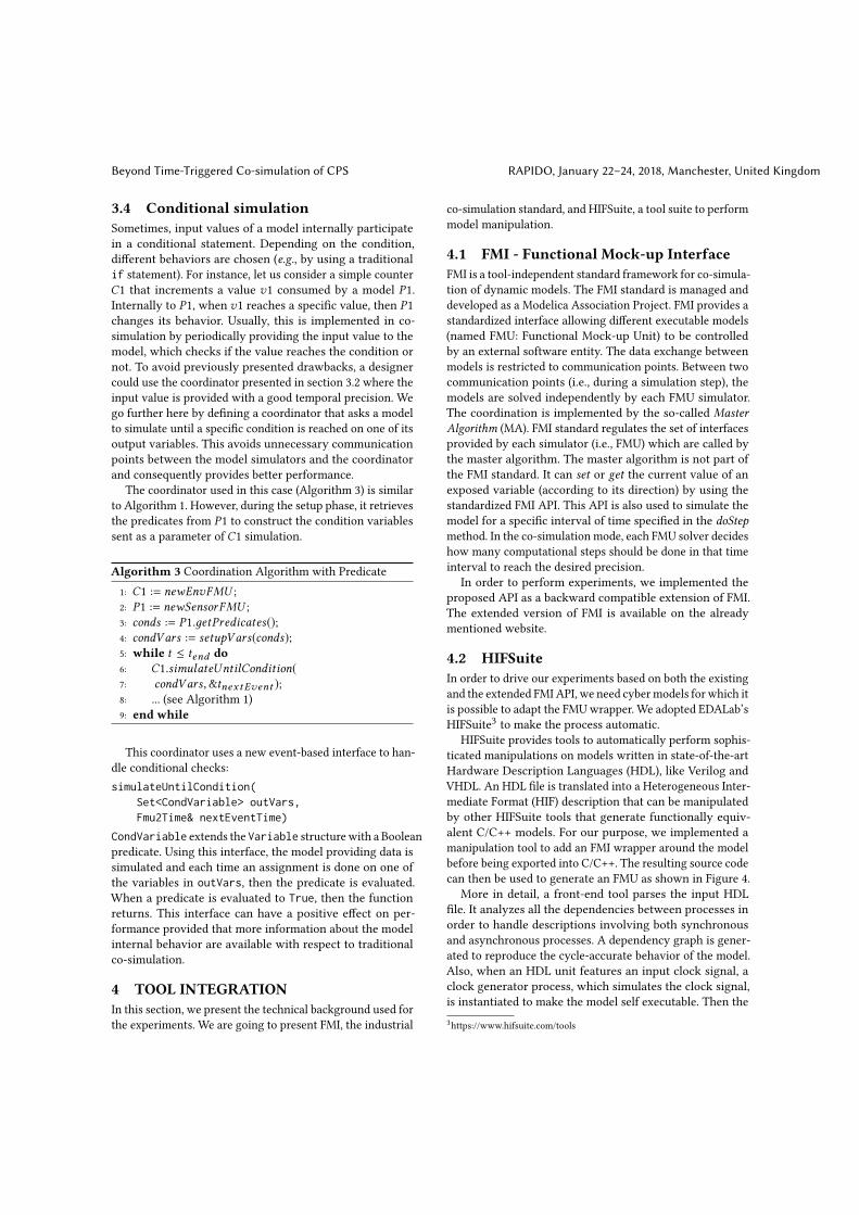
HIFSuite provides tools to automatically perform sophis-ticated manipulations on models written in state-of-the-artHardware Description Languages (HDL), like Verilog andVHDL. An HDL file is translated into a Heterogeneous Inter-mediate Format (HIF) description that can be manipulatedby other HIFSuite tools that generate functionally equiv-alent C/C++ models. For our purpose, we implemented amanipulation tool to add an FMI wrapper around the modelbefore being exported into C/C++. The resulting source codecan then be used to generate an FMU as shown in Figure 4.

More in detail, a front-end tool parses the input HDLfile. It analyzes all the dependencies between processes inorder to handle descriptions involving both synchronousand asynchronous processes. A dependency graph is gener-ated to reproduce the cycle-accurate behavior of the model.Also, when an HDL unit features an input clock signal, aclock generator process, which simulates the clock signal,is instantiated to make the model self executable. Then the3https://www.hifsuite.com/tools

RAPIDO, January 22–24, 2018, Manchester, United Kingdom G. Liboni et al.

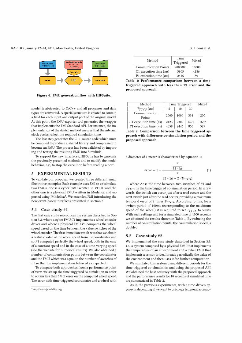
Figure 4: FMU generation flow with HIFSuite.

model is abstracted to C/C++ and all processes and datatypes are converted. A special structure is created to containa field for each input and output port of the original model.At this point, the FMU exporter tool generates the wrapperthat implements the FMI Standard API. For instance, the im-plementation of the doStep method ensures that the internalclock cycles reflect the required simulation time.

The last step generates the C++ source code which mustbe compiled to produce a shared library and compressed tobecome an FMU. The process has been validated by import-ing and testing the resulting FMU into Simulink.

To support the new interfaces, HIFSuite has to generatethe previously presented methods and to modify the modelbehavior, e.g., to stop the execution before reading a port.

5 EXPERIMENTAL RESULTSTo validate our proposal, we created three different smallillustrative examples. Each example uses FMI to co-simulatetwo FMUs, one is a cyber FMU written in VHDL and theother one is a physical FMU written in Modelica and ex-ported using JModelica4. We extended FMI introducing thenew event-based interfaces presented in section 3.

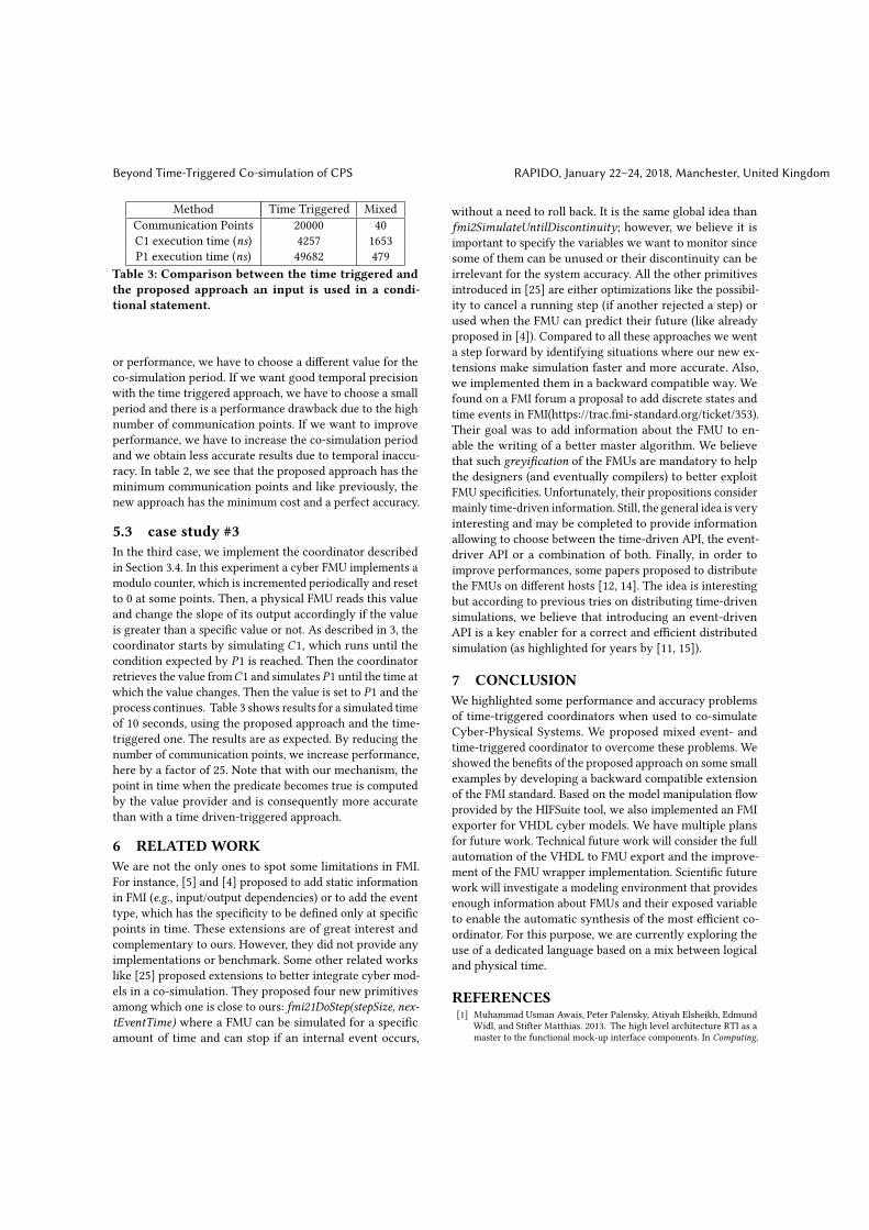
5.1 Case study #1The first case study reproduces the system described in Sec-tion 3.2, where a cyber FMUC1 implements a wheel encoderdriver and where a physical FMU P1 computes the wheelspeed based on the time between the value switches of thewheel encoder. The first immediate result was that we obtaina realistic value of the wheel speed from the coordinator andso P1 computed perfectly the wheel speed, both in the caseof a constant speed and in the case of a time-varying speed(see the website for numerical results). We also obtained anumber of communication points between the coordinatorand the FMU which was equal to the number of switches ofv1 so that the implementation behaved as expected.

To compare both approaches from a performance pointof view, we set up the time-triggered co-simulation in orderto obtain less than 1% of error on the computed wheel speed.The error with time-triggered coordinator and a wheel with

4http://www.jmodelica.org

Method TimeTriggered Mixed

Communication Points 2000000 10000C1 execution time (ms) 5805 4186P1 execution time (ms) 2455 89

Table 1: Performance comparison between a time-triggered approach with less than 1% error and theproposed approach.

Method Time Triggered MixedTTTCS (ms) 5 10 30

CommunicationPoints 2000 1000 334 200

C1 execution time (ns) 2123 2309 1491 1667P1 execution time (ns) 4058 2446 850 529

Table 2: Comparison between the time triggered ap-proach with difference co-simulation period and theproposed approach.

a diameter of 1 meter is characterized by equation 1:

error = 1 −π

32 · ∆tπ

32 · (∆t − 2 ·TTTCS )

(1)

where ∆t is the time between two switches of v1 andTTTCS is the time triggered co-simulation period. In a fewwords, the switch can occur just after a read occurs and thenext switch just after the read occurs, providing a maximumtemporal error of 2 times TTTCS . According to this, for aswitch period of 100ms (corresponding to the maximumspeed of the wheel) it is required to set TTTCS to 500ns.With such settings and for a simulated time of 1000 secondswe obtained the results shown in Table 1. By reducing thenumber of co-simulation points, the co-simulation speed isdoubled.

5.2 Case study #2We implemented the case study described in Section 3.3,i.e., a system composed by a physical FMU that implementsthe temperature of an environment and a cyber FMU thatimplements a sensor driver. It reads periodically the value ofthe environment and then uses it for further computation.

We simulated this system using different periods for thetime triggered co-simulation and using the proposed API.We obtained the best accuracy with the proposed approachand the performance results for 10 seconds of simulated timeare summarized in Table 2.

As in the previous experiments, with a time-driven ap-proach, depending if we want to privilege temporal accuracy

Beyond Time-Triggered Co-simulation of CPS RAPIDO, January 22–24, 2018, Manchester, United Kingdom

Method Time Triggered MixedCommunication Points 20000 40C1 execution time (ns) 4257 1653P1 execution time (ns) 49682 479

Table 3: Comparison between the time triggered andthe proposed approach an input is used in a condi-tional statement.

or performance, we have to choose a different value for theco-simulation period. If we want good temporal precisionwith the time triggered approach, we have to choose a smallperiod and there is a performance drawback due to the highnumber of communication points. If we want to improveperformance, we have to increase the co-simulation periodand we obtain less accurate results due to temporal inaccu-racy. In table 2, we see that the proposed approach has theminimum communication points and like previously, thenew approach has the minimum cost and a perfect accuracy.

5.3 case study #3In the third case, we implement the coordinator describedin Section 3.4. In this experiment a cyber FMU implements amodulo counter, which is incremented periodically and resetto 0 at some points. Then, a physical FMU reads this valueand change the slope of its output accordingly if the valueis greater than a specific value or not. As described in 3, thecoordinator starts by simulating C1, which runs until thecondition expected by P1 is reached. Then the coordinatorretrieves the value fromC1 and simulates P1 until the time atwhich the value changes. Then the value is set to P1 and theprocess continues. Table 3 shows results for a simulated timeof 10 seconds, using the proposed approach and the time-triggered one. The results are as expected. By reducing thenumber of communication points, we increase performance,here by a factor of 25. Note that with our mechanism, thepoint in time when the predicate becomes true is computedby the value provider and is consequently more accuratethan with a time driven-triggered approach.

6 RELATED WORKWe are not the only ones to spot some limitations in FMI.For instance, [5] and [4] proposed to add static informationin FMI (e.g., input/output dependencies) or to add the eventtype, which has the specificity to be defined only at specificpoints in time. These extensions are of great interest andcomplementary to ours. However, they did not provide anyimplementations or benchmark. Some other related workslike [25] proposed extensions to better integrate cyber mod-els in a co-simulation. They proposed four new primitivesamong which one is close to ours: fmi21DoStep(stepSize, nex-tEventTime) where a FMU can be simulated for a specificamount of time and can stop if an internal event occurs,

without a need to roll back. It is the same global idea thanfmi2SimulateUntilDiscontinuity; however, we believe it isimportant to specify the variables we want to monitor sincesome of them can be unused or their discontinuity can beirrelevant for the system accuracy. All the other primitivesintroduced in [25] are either optimizations like the possibil-ity to cancel a running step (if another rejected a step) orused when the FMU can predict their future (like alreadyproposed in [4]). Compared to all these approaches we wenta step forward by identifying situations where our new ex-tensions make simulation faster and more accurate. Also,we implemented them in a backward compatible way. Wefound on a FMI forum a proposal to add discrete states andtime events in FMI(https://trac.fmi-standard.org/ticket/353).Their goal was to add information about the FMU to en-able the writing of a better master algorithm. We believethat such greyification of the FMUs are mandatory to helpthe designers (and eventually compilers) to better exploitFMU specificities. Unfortunately, their propositions considermainly time-driven information. Still, the general idea is veryinteresting and may be completed to provide informationallowing to choose between the time-driven API, the event-driver API or a combination of both. Finally, in order toimprove performances, some papers proposed to distributethe FMUs on different hosts [12, 14]. The idea is interestingbut according to previous tries on distributing time-drivensimulations, we believe that introducing an event-drivenAPI is a key enabler for a correct and efficient distributedsimulation (as highlighted for years by [11, 15]).

7 CONCLUSIONWe highlighted some performance and accuracy problemsof time-triggered coordinators when used to co-simulateCyber-Physical Systems. We proposed mixed event- andtime-triggered coordinator to overcome these problems. Weshowed the benefits of the proposed approach on some smallexamples by developing a backward compatible extensionof the FMI standard. Based on the model manipulation flowprovided by the HIFSuite tool, we also implemented an FMIexporter for VHDL cyber models. We have multiple plansfor future work. Technical future work will consider the fullautomation of the VHDL to FMU export and the improve-ment of the FMU wrapper implementation. Scientific futurework will investigate a modeling environment that providesenough information about FMUs and their exposed variableto enable the automatic synthesis of the most efficient co-ordinator. For this purpose, we are currently exploring theuse of a dedicated language based on a mix between logicaland physical time.

REFERENCES[1] Muhammad Usman Awais, Peter Palensky, Atiyah Elsheikh, Edmund

Widl, and Stifter Matthias. 2013. The high level architecture RTI as amaster to the functional mock-up interface components. In Computing,

RAPIDO, January 22–24, 2018, Manchester, United Kingdom G. Liboni et al.

Networking and Communications (ICNC), 2013 International Conferenceon. IEEE, 315–320.

[2] Jens Bastian, Christop Clauß, Susann Wolf, and Peter Schneider. 2011.Master for co-simulation using FMI. In Proceedings of the 8th Inter-national Modelica Conference; March 20th-22nd; Technical Univeristy;Dresden; Germany. Linköping University Electronic Press, 115–120.

[3] Frédéric Boussinot and Robert De Simone. 1991. The ESTEREL language.Proc. IEEE 79, 9 (1991), 1293–1304.

[4] David Broman, Christopher Brooks, Lev Greenberg, Edward A Lee,Michael Masin, Stavros Tripakis, and Michael Wetter. 2013. Determinatecomposition of FMUs for co-simulation. In Proceedings of the EleventhACM International Conference on Embedded Software. IEEE Press, 2.

[5] David Broman, Lev Greenberg, Edward A. Lee, Michael Masin, StavrosTripakis, and Michael Wetter. 2014. Requirements for Hybrid Cosimu-lation. Technical Report UCB/EECS-2014-157. EECS Department, Uni-versity of California, Berkeley. to appear in HSCC, Seattle, WA, April14-16, 2015.

[6] Stefano Centomo, Julien Deantoni, and Robert De Simone. 2016. UsingSystemC Cyber Models in an FMI Co-Simulation Environment. In 19thEuromicro Conference on Digital System Design 31 August - 2 Septem-ber 2016 (19th Euromicro Conference on Digital System Design), Vol. 19.Limassol, Cyprus. https://doi.org/10.1109/DSD.2016.86

[7] Benoit Combemale, Cédric Brun, Joël Champeau, Xavier Crégut, JulienDeantoni, and Jérome Le Noir. 2016. A Tool-Supported Approach forConcurrent Execution of Heterogeneous Models. In 8th European Con-gress on Embedded Real Time Software and Systems (ERTS 2016).

[8] Benoit Combemale, Julien Deantoni, Benoit Baudry, Robert B. France,Jean-Marc Jézéquel, and Jeff Gray. 2014. Globalizing Modeling Lan-guages. IEEE Computer (June 2014), 10–13. https://hal.inria.fr/hal-00994551

[9] Fabio Cremona, Marten Lohstroh, Stavros Tripakis, Christopher Brooks,and Edward A. Lee. 2016. FIDE - An FMI Integrated DevelopmentEnvironment. In Symposium on Applied Computing.

[10] Julien Deantoni, Cédric Brun, Benoit Caillaud, Robert B. France, GaborKarsai, Oscar Nierstrasz, and Eugene Syriani. 2015. Domain Global-ization: Using Languages to Support Technical and Social Coordination.Springer International Publishing, Cham, 70–87. https://doi.org/10.1007/978-3-319-26172-0_5

[11] Colin Fidge. 1991. Logical time in distributed computing systems. Com-puter 24, 8 (1991), 28–33.

[12] Virginie Galtier, Stephane Vialle, Cherifa Dad, Jean-Philippe Tavella,Jean-Philippe Lam-Yee-Mui, and Gilles Plessis. 2015. FMI-based Dis-tributed Multi-simulation with DACCOSIM. In Proceedings of the Sym-posium on Theory of Modeling & Simulation: DEVS Integrative M&SSymposium (DEVS ’15). Society for Computer Simulation International,San Diego, CA, USA, 39–46.

[13] David Garlan and Mary Shaw. 1993. An introduction to software archi-tecture. Advances in software engineering and knowledge engineering 1,3.4 (1993).

[14] Abir Ben Khaled, Mongi Ben Gaid, Nicolas Pernet, and Daniel Simon.2014. Fast multi-core co-simulation of Cyber-Physical Systems: Applica-tion to internal combustion engines. Simulation Modelling Practice andTheory 47 (2014), 79 – 91. https://doi.org/10.1016/j.simpat.2014.05.002

[15] Leslie Lamport. 1978. Time, clocks, and the ordering of events in adistributed system. Commun. ACM 21, 7 (1978), 558–565.

[16] Matias Ezequiel Vara Larsen, Julien Deantoni, Benoit Combemale, andFrédéric Mallet. 2015. A behavioral coordination operator language(BCOoL). InModel Driven Engineering Languages and Systems (MODELS),2015 ACM/IEEE 18th International Conference on. IEEE, 186–195.

[17] Matias Ezequiel Vara Larsen, Julien Deantoni, Benoit Combemale, andFrédéric Mallet. 2015. A Model-Driven Based Environment for Auto-matic Model Coordination. In Models 2015 demo and posters.

[18] Edward A Lee. 2008. Cyber physical systems: Design challenges. InObject Oriented Real-Time Distributed Computing (ISORC), 2008 11th IEEEInternational Symposium on. IEEE, 363–369.

[19] Nenad Medvidovic and Richard N Taylor. 1997. A framework for classi-fying and comparing architecture description languages. ACM SIGSOFTSoftware Engineering Notes 22, 6 (1997), 60–76.

[20] Modelisar. 2014. FMI for Model Exchange and Co-Simulation. (July2014). https://fmi-standard.org/downloads#version2

[21] Himanshu Neema, Jesse Gohl, Zsolt Lattmann, Janos Sztipanovits, GaborKarsai, Sandeep Neema, Ted Bapty, John Batteh, Hubertus Tummescheit,and Chandraseka Sureshkumar. 2014. Model-based integration platform

for FMI co-simulation and heterogeneous simulations of cyber-physicalsystems. In Proceedings of the 10 th International Modelica Conference;Lund; Sweden. Linköping University Electronic Press, 235–245.

[22] George A Papadopoulos and Farhad Arbab. 1998. Coordination modelsand languages. Advances in computers 46 (1998), 329–400.

[23] Vitaly Savicks, Michael Butler, and John Colley. 2014. Co-simulatingEvent-B and continuous models via FMI. In Proceedings of the 2014Summer Simulation Multiconference. Society for Computer SimulationInternational, 37.

[24] Tom Schierz, Martin Arnold, and Christoph Clauß. 2012. Co-simulationwith communication step size control in an FMI compatible masteralgorithm. In Proceedings of the 9th International MODELICA Conference;Munich; Germany. Linköping University Electronic Press, 205–214.

[25] Jean-Philippe Tavella, Mathieu Caujolle, Charles Tan, Gilles Plessis,Mathieu Schumann, Stéphane Vialle, Cherifa Dad, Arnaud Cuccuru, andSébastien Revol. 2016. Toward an Hybrid Co-simulation with the FMI-CS Standard. (April 2016). https://hal-centralesupelec.archives-ouvertes.fr/hal-01301183 Research Report.

[26] S. Tripakis. 2015. Bridging the semantic gap between heterogeneousmodeling formalisms and FMI. In 2015 International Conference onEmbedded Computer Systems: Architectures, Modeling, and Simulation(SAMOS). 60–69. https://doi.org/10.1109/SAMOS.2015.7363660

[27] Bert Van Acker, Joachim Denil, Hans Vangheluwe, and Paul De Meu-lenaere. 2015. Generation of an Optimised Master Algorithm for FMICo-simulation. In Proceedings of the Symposium on Theory of Modeling& Simulation: DEVS Integrative M&S Symposium (DEVS ’15). Society forComputer Simulation International, San Diego, CA, USA, 205–212.

[28] Baobing Wang and John S. Baras. 2013. HybridSim: A Modeling andCo-simulation Toolchain for Cyber-physical Systems. In Proceedings ofthe 2013 IEEE/ACM 17th International Symposium on Distributed Simu-lation and Real Time Applications (DS-RT ’13). IEEE Computer Society,Washington, DC, USA, 33–40. https://doi.org/10.1109/DS-RT.2013.12

XXII

Real-Time Capable Retargeting ofXilinx MicroBlaze Binaries usingQEMU

XXIII

Real-Time Capable Retargeting of Xilinx MicroBlazeBinaries using QEMU – A Feasibility Study

Irune Yarza Mikel Azkarate-askasua

IK4-Ikerlan Technology Research Centre, Dependable Embedded SystemsPo J.M. Arizmendiarrieta, 2

20500 Arrasate-Mondragón, Spainiyarza@ikerlan.es, emailmazkarateaskasua@ikerlan.es

Kim GrüttnerOFFIS - Institute for

Information TechnologyEschwerweg 2

26121 Oldenburg, Germanykim.gruettner@offis.de

Wolfgang NebelC.v.O. Universität Oldenburg

Ammerländer Heerstr.114-118

26121 Oldenburg, Germanynebel@informatik.uni-

oldenburg.de

ABSTRACTThe great expansion and fast evolution of embedded systems mar-ket and the known advantages of the use of multi-core processorsin this area are generating interest on improved embedded systemstechnologies (e.g., shrinking transistor size, new on-chip architec-tures), which at the same time are shortening the obsolescence pe-riods of the underlying hardware. As a consequence, software de-signed for those platforms (a.k.a legacy code), that might be func-tionally correct and validated code, will be lost when changingthe underlying Instruction Set Architecture (ISA) and peripherals.Given that many embedded systems execute Real-Time (RT) ap-plications, the legacy code migration problem directly affects RTsystems. Dynamic Binary Translation (DBT) techniques have beenwidely used for the migration of legacy code to a new hardwareplatform. However, there are no works which consider their use forRT legacy code migration. Therefore, this paper analyzes the suit-ability of a DBT based emulator, Quick EMUlator (QEMU), as amean for RT legacy code migration, mainly focusing on its tempo-ral capacities. To this end, a test framework has been constructed tocheck and compare the timing behavior of a bare-metal executionon a Xilinx MicroBlaze processor against a QEMU emulated Mi-croBlaze running on an ARM Cortex-A9 processor. Results showthat the proposed approach could provide hard RT performance in55% and soft RT performance in 74% of our considered bench-marks.

KeywordsDynamic Binary Translation, legacy code, Real-Time Systems, re-targeting

Permission to make digital or hard copies of all or part of this work for personal orclassroom use is granted without fee provided that copies are not made or distributedfor profit or commercial advantage and that copies bear this notice and the full cita-tion on the first page. Copyrights for components of this work owned by others thanACM must be honored. Abstracting with credit is permitted. To copy otherwise, or re-publish, to post on servers or to redistribute to lists, requires prior specific permissionand/or a fee. Request permissions from permissions@acm.org.

RAPIDO, January 22–24, 2018, Manchester, United Kingdom© 2018 ACM. ISBN 978-1-4503-6417-1/18/01. . . $15.00

DOI: https://doi.org/10.1145/3180665.3180671

1. INTRODUCTIONNext generation embedded systems must provide better per-

formance, increased dependability, and energy efficiency, whileachieving a cost effective product withing a reduced time-to-market. This transition is being encouraged by the important roleof multi-core processors in the area of embedded systems, provid-ing concurrent resources and increased performance rates at lowerclock frequencies and lower power consumption [7].

The continuous demand for improved embedded system tech-nologies and the fact that processor manufacturers are universallymoving to multi-core solutions has provoked the shortening of theobsolescence period of embedded systems hardware and, as a con-sequence, the need to deal with legacy code. Legacy code is char-acterized by some particular properties: usually runs on obsoletehardware which is slow and expensive to maintain [23], has no oroutdated documentation [21], and is essential for the company [5]since it comprises business knowledge [22].

Due to the fact that classical process models focus on the firststage of software life cycle (development) instead of operation ormaintenance stages, the process of updating legacy systems is usu-ally complex, error-prone, time consuming and requires high costinvestments. One of the existing forms to deal with legacy codeis binary translation. The aim of binary translation is to transformexisting binaries (for the legacy ISA) into binaries for the new ar-chitecture, either statically or dynamically (during emulation). Thisway, the legacy system is transformed into a new form that will im-prove its operation, system capability, functionality, performanceor evolvability at a lower cost, schedule or risk to the customer[19].

1.1 MotivationIndustry needs a RT software re-targeting approach that can be

easily ported to different target and host processors and we seebinary translation technologies as a good candidate to implementthose needs. Although binary translation techniques have been suc-cessfully applied to non-RT applications, only [11] and [15] con-sider RT systems in their proposed approaches. When dealing withthe migration process of legacy RT systems, not only the functionalbehavior of the software, but also the temporal behavior has to be

preserved. This is a typical pattern of a reactive RT system, foundin many control applications. One example is a plant controllersystem, where the controller is periodically triggered, obtains new(sensor) data and updates its (actuator) outputs within a specificperiod of time, which has to be smaller than its triggering period.

1.2 ContributionsThe overall goal of this research is to enable the migration of

RT embedded legacy code to a new hardware platform with guar-anteed RT performance. This paper describes the first steps of thisresearch. To this end, this work analyzes the suitability of QEMU,as a machine-adaptable DBT tool, for its use in a RT property con-serving re-targeting process. This approach is applicable when theoriginal source-code is not available or there is a need to keep itunmodified.

The main contribution of this paper is the construction of a testenvironment to check if the timing behavior on the legacy archi-tecture can be fulfilled on the new architecture. Due to the multi-host and -target quality of QEMU, our proposed test framework caneasily be ported and used in other guest/host combinations. The de-tailed technical contributions of this paper are:• Overview of the state of the art in static and dynamic code

translation techniques heeding portability, embedded sys-tems or RT legacy code.• Establishment of a Xilinx MircoBlaze QEMU environment

on a Xilinx Zynq ARM Cortex-A9 processing system.• Setup of a high-resolution execution time measurement for

periodically triggered software running on QEMU.• A feasibility study for RT capable re-targeting of Xilinx

MicroBlaze binaries using QEMU on a Xilinx Zynq ARMCortex-A9 processing system.

1.3 OutlineThe remainder of the paper is organized as follows. An overview

of related work in the area of machine-adaptable static and dynamiccode translation techniques for embedded systems is provided inSection 2. Then, Section 3 presents the proposed solution and de-scribes the implementation details of the MircoBlaze QEMU en-vironment on a Xilinx Zynq ARM Cortex-A9 processing system.Section 4 describes the construction of the test framework with ahigh-resolution execution time measurement of a periodically trig-gered software. Section 5 executes the feasibility study and dis-cusses the experimental results. An outlook on future work and aconclusion is given in Section 6.

2. RELATED WORKBinary translation techniques have been widely studied and de-

veloped in the last two decades. Some of the utilities of binarytranslation techniques include fast simulation of instruction sets, re-source protection and management (safety), and software securityenforcement. Moreover, binary translation appears to be a standardapproach for legacy software migration, as the software that runson the legacy hardware can be migrated to a new hardware plat-form without a considerable expense of time, effort and money.

The first binary translation techniques were developed in the late1980s for academic researches and commercial products [10]. In1987, HP developed one of the earliest commercial binary transla-tion systems to migrate source HP 3000 programs to the new Preci-sion Architecture [6]. Followed by the IBM System/370 simulatorrunning on top of an IBM RT(RISC) PC, MIMIC [17]. Later, bi-nary translation techniques were used by many other affiliationsaiming a migration path for existing software.

Software based binary translation systems can be classified into

two categories: Static Binary Translation (SBT) and DBT. Theformer translates the binary code offline, before the program is ex-ecuted, while the later translates the binary code at runtime, duringprogram execution.

Nowadays, most binary translation approaches adopt dynamictranslation, since this technique can easily handle indirect branchesand can perform optimization based on program’s run-time behav-ior. However, as translation and optimization time counts for a partof the execution time (which incurs execution overhead), dynamictranslation approaches cannot perform aggressive optimizations.On the contrary, static translation approaches can perform wholeprogram optimization without influence on run-time overhead butthey must deal with code discovery, code location and self modi-fying code issues. Some researches have even implemented hybridbinary translation techniques to take advantage of the strengths ofboth methods.

Given the great amount of binary translation systems, just thoseheeding portability, embedded systems and/or RT applications willbe considered here.

2.1 Static Binary TranslationThe TIBBIT project [11] was the first binary translation ap-

proach developed for embedded RT applications (which are not as-sumed to be user-level processes) that needed to be migrated to adifferent processor but still maintaining the externally observabletiming behavior. To this end, both, the legacy application and theoperating system code, used by the application, are packed in ablack box that is executed on top of the host operating system.During the translation process, timing code is inserted into eachtranslation block, to maintain the timing behavior the same as inthe original processor. If the execution is running faster than it didin the old processor, other tasks are run until the execution is backon schedule.

The UQBT [9] was the first SBT tool designed with portability inmind. UQBT translates the user-level target binary into a Higher-Level Register Transfer Language (HRTL), which is a machine-independent representation, and then the HRTL is translated intohost machine binary code, what makes the tool easily and inex-pensively portable to new target and host architectures. To handleindirect calls that could not be discovered at static time, the UQBTuses an interpreter.

Chen et al. [8] developed a SBT solution for embedded systems.Their tool directly migrated ARM binaries to a MIPS-like archi-tecture, without using an Intermediate Representation (IR), whichenabled applying architecture specific optimization but at the sametime hindered translator’s retargetability. Their translation tool wasable to migrate user-level ARM binaries without using a run-timeemulator or DBT support.

Heinz [15] proposed a system-level SBT approach for the migra-tion of RT legacy software. However, instead of dynamically com-puting a delay, as Cowsgell and Zary did on the TIBBIT project,the computation of the delay is shifted from run-time to compile-time. The translator selects from a set of precomputed delays theappropriate value according to the context of a program point, sothere is no need to keep track of the execution time on the sourcemachine.

DisIRer [16] is a multi-platform SBT tool based on the GNUCompiler Collection (GCC) compiler infrastructure. DisIRer con-verts user-mode target binary programs into GCC IR and thentranslates IR into host binary code using GCC optimizer and backend. The fact that it is based on GCC makes the translator costeffective and retargetable.

Shen et al. [18] worked out a Low Level Virtual Machine

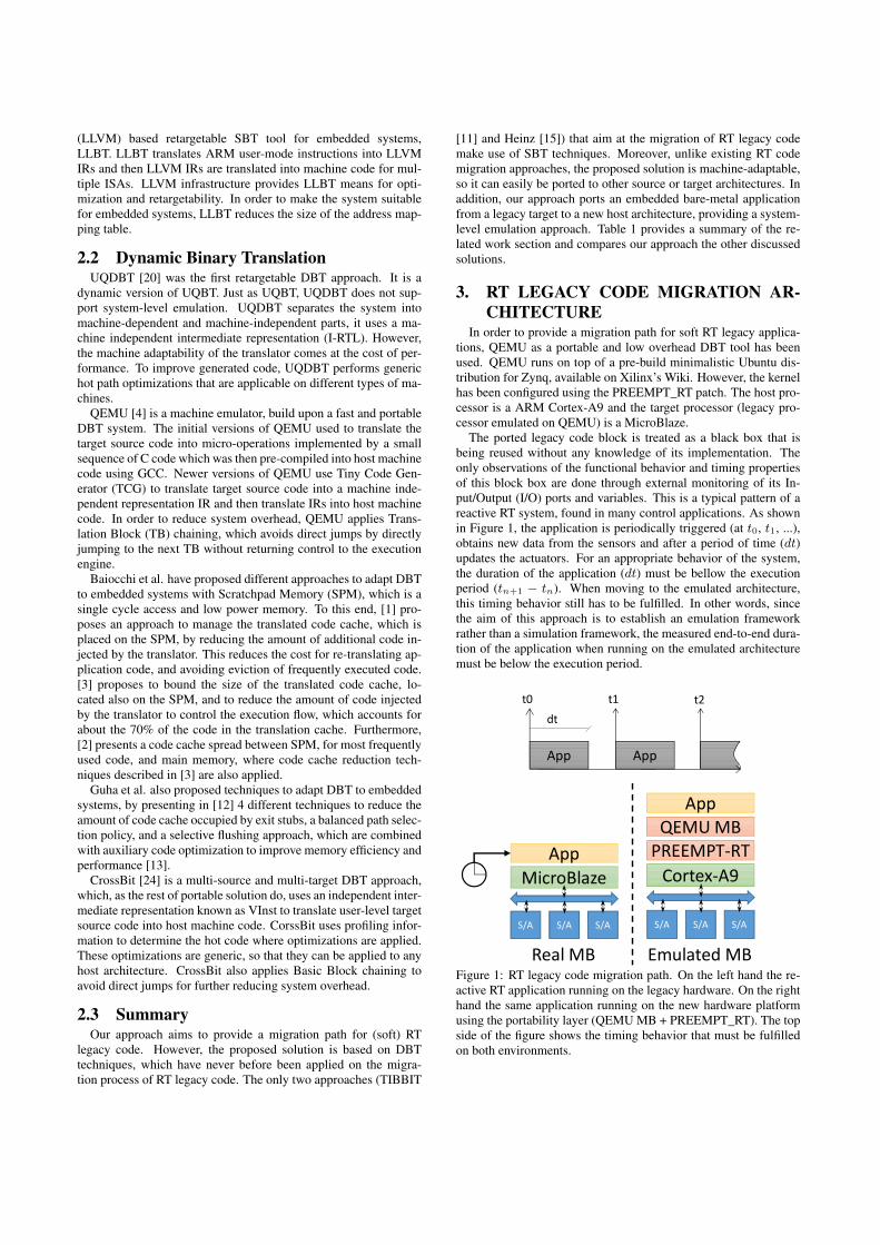
(LLVM) based retargetable SBT tool for embedded systems,LLBT. LLBT translates ARM user-mode instructions into LLVMIRs and then LLVM IRs are translated into machine code for mul-tiple ISAs. LLVM infrastructure provides LLBT means for opti-mization and retargetability. In order to make the system suitablefor embedded systems, LLBT reduces the size of the address map-ping table.

2.2 Dynamic Binary TranslationUQDBT [20] was the first retargetable DBT approach. It is a

dynamic version of UQBT. Just as UQBT, UQDBT does not sup-port system-level emulation. UQDBT separates the system intomachine-dependent and machine-independent parts, it uses a ma-chine independent intermediate representation (I-RTL). However,the machine adaptability of the translator comes at the cost of per-formance. To improve generated code, UQDBT performs generichot path optimizations that are applicable on different types of ma-chines.

QEMU [4] is a machine emulator, build upon a fast and portableDBT system. The initial versions of QEMU used to translate thetarget source code into micro-operations implemented by a smallsequence of C code which was then pre-compiled into host machinecode using GCC. Newer versions of QEMU use Tiny Code Gen-erator (TCG) to translate target source code into a machine inde-pendent representation IR and then translate IRs into host machinecode. In order to reduce system overhead, QEMU applies Trans-lation Block (TB) chaining, which avoids direct jumps by directlyjumping to the next TB without returning control to the executionengine.

Baiocchi et al. have proposed different approaches to adapt DBTto embedded systems with Scratchpad Memory (SPM), which is asingle cycle access and low power memory. To this end, [1] pro-poses an approach to manage the translated code cache, which isplaced on the SPM, by reducing the amount of additional code in-jected by the translator. This reduces the cost for re-translating ap-plication code, and avoiding eviction of frequently executed code.[3] proposes to bound the size of the translated code cache, lo-cated also on the SPM, and to reduce the amount of code injectedby the translator to control the execution flow, which accounts forabout the 70% of the code in the translation cache. Furthermore,[2] presents a code cache spread between SPM, for most frequentlyused code, and main memory, where code cache reduction tech-niques described in [3] are also applied.

Guha et al. also proposed techniques to adapt DBT to embeddedsystems, by presenting in [12] 4 different techniques to reduce theamount of code cache occupied by exit stubs, a balanced path selec-tion policy, and a selective flushing approach, which are combinedwith auxiliary code optimization to improve memory efficiency andperformance [13].

CrossBit [24] is a multi-source and multi-target DBT approach,which, as the rest of portable solution do, uses an independent inter-mediate representation known as VInst to translate user-level targetsource code into host machine code. CorssBit uses profiling infor-mation to determine the hot code where optimizations are applied.These optimizations are generic, so that they can be applied to anyhost architecture. CrossBit also applies Basic Block chaining toavoid direct jumps for further reducing system overhead.

2.3 SummaryOur approach aims to provide a migration path for (soft) RT

legacy code. However, the proposed solution is based on DBTtechniques, which have never before been applied on the migra-tion process of RT legacy code. The only two approaches (TIBBIT

[11] and Heinz [15]) that aim at the migration of RT legacy codemake use of SBT techniques. Moreover, unlike existing RT codemigration approaches, the proposed solution is machine-adaptable,so it can easily be ported to other source or target architectures. Inaddition, our approach ports an embedded bare-metal applicationfrom a legacy target to a new host architecture, providing a system-level emulation approach. Table 1 provides a summary of the re-lated work section and compares our approach the other discussedsolutions.

3. RT LEGACY CODE MIGRATION AR-CHITECTURE

In order to provide a migration path for soft RT legacy applica-tions, QEMU as a portable and low overhead DBT tool has beenused. QEMU runs on top of a pre-build minimalistic Ubuntu dis-tribution for Zynq, available on Xilinx’s Wiki. However, the kernelhas been configured using the PREEMPT_RT patch. The host pro-cessor is a ARM Cortex-A9 and the target processor (legacy pro-cessor emulated on QEMU) is a MicroBlaze.

The ported legacy code block is treated as a black box that isbeing reused without any knowledge of its implementation. Theonly observations of the functional behavior and timing propertiesof this block box are done through external monitoring of its In-put/Output (I/O) ports and variables. This is a typical pattern of areactive RT system, found in many control applications. As shownin Figure 1, the application is periodically triggered (at t0, t1, ...),obtains new data from the sensors and after a period of time (dt)updates the actuators. For an appropriate behavior of the system,the duration of the application (dt) must be bellow the executionperiod (tn+1 − tn). When moving to the emulated architecture,this timing behavior still has to be fulfilled. In other words, sincethe aim of this approach is to establish an emulation frameworkrather than a simulation framework, the measured end-to-end dura-tion of the application when running on the emulated architecturemust be below the execution period.

App

t0 t1

App

dt

t2

MicroBlaze

S/A S/A S/A

AppCortex-A9

S/A S/A S/A

QEMU MBApp

PREEMPT-RT

Real MB Emulated MBFigure 1: RT legacy code migration path. On the left hand the re-active RT application running on the legacy hardware. On the righthand the same application running on the new hardware platformusing the portability layer (QEMU MB + PREEMPT_RT). The topside of the figure shows the timing behavior that must be fulfilledon both environments.

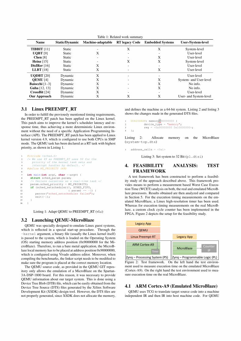
Table 1: Related work summary

Name Static/Dynamic Machine-adaptable RT legacy Code Embedded Systems User-/System-level

TIBBIT [11] Static - X X System-levelUQBT [9] Static X - - User-levelChen [8] Static - - X User-level

Heinz [15] Static - X X System-levelDisIRer [16] Static X - - User-levelLLBT [18] Static X - X User-level

UQDBT [20] Dynamic X - - User-levelQEMU [4] Dynamic X - X System- and User-level

Baiocchi [1–3] Dynamic X - X No info.Guha [12, 13] Dynamic X - X No info.CrossBit [24] Dynamic X - - User-level

Our Approach Dynamic X X X User- and System-level

3.1 Linux PREEMPT_RTIn order to fulfill the previously mentioned timing requirements,

the PREEMPT_RT patch has been applied on the Linux kernel.This patch aims to improve the kernel’s scheduler latency and re-sponse time, thus achieving a more deterministic Linux environ-ment without the need of a specific Application Programming In-terface (API). The PREEMPT_RT patch has been applied to Linuxkernel version 4.9, which is configured to use both CPUs in SMPmode. The QEMU task has been declared as a RT task with highestpriority, as shown in Listing 1.

1 #include <sched.h>2 /* We use 49 as PREEMPT_RT uses 50 for the3 priority of the kernel task sets and4 interrupt handler by default. */5 #define MY_PRIORITY (49)6

7 int main(int argc, char **argv) {8 struct sched_param param;9 /* Declare ourselves as a real-time task */

10 param.sched_priority = MY_PRIORITY;11 if (sched_setscheduler(0, SCHED_FIFO,12 & param) == -1) {13 perror("sched_setscheduler failed");14 exit(-1);15 }16 }

Listing 1: Adapt QEMU to PREEMPT_RT (vl.c)

3.2 Launching QEMU-MicroBlazeQEMU was specially designed to emulate Linux guest systems,

which is reflected in a special start-up procedure. Through the-kernel argument, a binary file (usually the Linux kernel itself)is passed to the system, which is loaded on the Operating System(OS) starting memory address position (0x90000000 for the Mi-croBlaze). Therefore, to run a bare metal application, the MicroB-laze local memory has to be placed at address position 0x90000000,which is configured using Vivado address editor. Moreover, whencompiling the benchmarks, the linker script needs to be modified tomake sure the program is placed at the correct memory location.

The QEMU source code, as provided in the QEMU GIT repos-itory only allows the emulation of a MicroBlaze on the Spartan-3A-DSP-1800 board. For this reason, it was necessary to provideQEMU information about our target system. This is done using aDevice Tree Blob (DTB) file, which can be easily obtained from theDevice Tree Source (DTS) files generated by the Xilinx SoftwareDevelopment Kit (XSDK) design tool. However, the DTS files arenot properly generated, since XSDK does not allocate the memory,

and defines the machine as a 64-bit system. Listing 2 and listing 3shows the changes made in the generated DTS files.

1 DDR2SDRAM: memory@90000000 {2 device_type = "memory";3 reg = <0x90000000 0x10000000>;4 };

Listing 2: Allocate memory on the MicroBlaze(system-top.dts)

1 address_cells = <0x1>

Listing 3: Set system to 32 Bit (pl.dtsi)

4. FEASIBILITY ANALYSIS: TESTFRAMEWORK

A test framework has been constructed to perform a feasibil-ity study of the approach described above. This framework pro-vides means to perform a measurement based Worst Case Execu-tion Time (WCET) analysis on both, the real and emulated MicroB-laze processors. Results obtained are then analyzed and comparedin Section 5. For the execution timing measurements on the em-ulated MicroBlaze, a Linux high-resolution timer has been used.Whereas for execution timing measurements on the real MicroB-laze, a custom clock cycle counter has been implemented in theFPGA. Figure 2 depicts the setup for the feasibility study.

ARM Cortex-A9

Linux Preempt-RT

QEMU

Zynq – Processing System (PS)

Legacy App

Timer

Zynq – Programmable Logic (PL)

PLPS

Legacy App

MicroBlazeCounter

IP

Figure 2: Test framework. On the left hand the test environ-ment used to measure execution time on the emulated MicroBlaze(Cortex-A9). On the right hand the test environment used to mea-sure execution time on the real MicroBlaze.

4.1 ARM Cortex-A9 (Emulated MicroBlaze)QEMU uses TCG to translate target source code into a machine

independent IR and then IR into host machine code. For QEMU

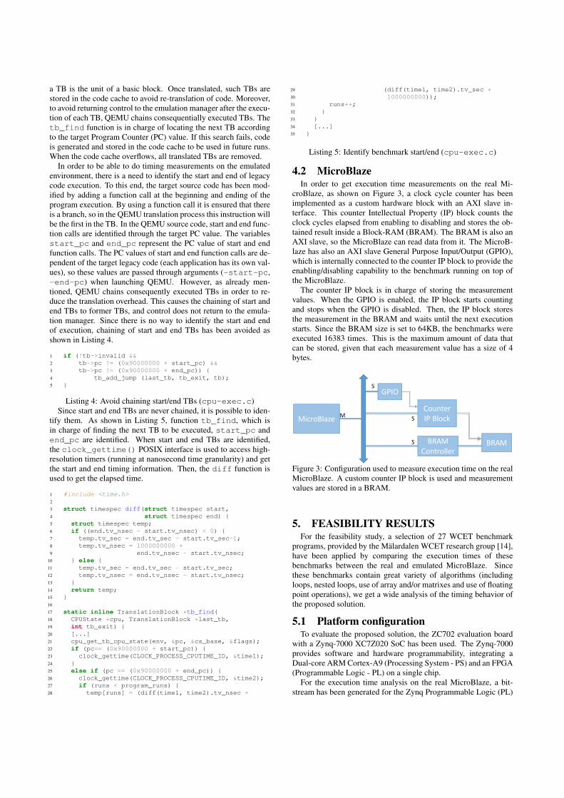
a TB is the unit of a basic block. Once translated, such TBs arestored in the code cache to avoid re-translation of code. Moreover,to avoid returning control to the emulation manager after the execu-tion of each TB, QEMU chains consequentially executed TBs. Thetb_find function is in charge of locating the next TB accordingto the target Program Counter (PC) value. If this search fails, codeis generated and stored in the code cache to be used in future runs.When the code cache overflows, all translated TBs are removed.

In order to be able to do timing measurements on the emulatedenvironment, there is a need to identify the start and end of legacycode execution. To this end, the target source code has been mod-ified by adding a function call at the beginning and ending of theprogram execution. By using a function call it is ensured that thereis a branch, so in the QEMU translation process this instruction willbe the first in the TB. In the QEMU source code, start and end func-tion calls are identified through the target PC value. The variablesstart_pc and end_pc represent the PC value of start and endfunction calls. The PC values of start and end function calls are de-pendent of the target legacy code (each application has its own val-ues), so these values are passed through arguments (-start-pc,-end-pc) when launching QEMU. However, as already men-tioned, QEMU chains consequently executed TBs in order to re-duce the translation overhead. This causes the chaining of start andend TBs to former TBs, and control does not return to the emula-tion manager. Since there is no way to identify the start and endof execution, chaining of start and end TBs has been avoided asshown in Listing 4.

1 if (!tb->invalid &&2 tb->pc != (0x90000000 + start_pc) &&3 tb->pc != (0x90000000 + end_pc)) {4 tb_add_jump (last_tb, tb_exit, tb);5 }

Listing 4: Avoid chaining start/end TBs (cpu-exec.c)Since start and end TBs are never chained, it is possible to iden-

tify them. As shown in Listing 5, function tb_find, which isin charge of finding the next TB to be executed, start_pc andend_pc are identified. When start and end TBs are identified,the clock_gettime() POSIX interface is used to access high-resolution timers (running at nanosecond time granularity) and getthe start and end timing information. Then, the diff function isused to get the elapsed time.

1 #include <time.h>2

3 struct timespec diff(struct timespec start,4 struct timespec end) {5 struct timespec temp;6 if ((end.tv_nsec - start.tv_nsec) < 0) {7 temp.tv_sec = end.tv_sec - start.tv_sec-1;8 temp.tv_nsec = 1000000000 +9 end.tv_nsec - start.tv_nsec;

10 } else {11 temp.tv_sec = end.tv_sec - start.tv_sec;12 temp.tv_nsec = end.tv_nsec - start.tv_nsec;13 }14 return temp;15 }16

17 static inline TranslationBlock *tb_find(18 CPUState *cpu, TranslationBlock *last_tb,19 int tb_exit) {20 [...]21 cpu_get_tb_cpu_state(env, &pc, &cs_base, &flags);22 if (pc== (0x90000000 + start_pc)) {23 clock_gettime(CLOCK_PROCESS_CPUTIME_ID, &time1);24 }25 else if (pc == (0x90000000 + end_pc)) {26 clock_gettime(CLOCK_PROCESS_CPUTIME_ID, &time2);27 if (runs < program_runs) {28 temp[runs] = (diff(time1, time2).tv_nsec +

29 (diff(time1, time2).tv_sec *30 1000000000));31 runs++;32 }33 }34 [...]35 }

Listing 5: Identify benchmark start/end (cpu-exec.c)

4.2 MicroBlazeIn order to get execution time measurements on the real Mi-

croBlaze, as shown on Figure 3, a clock cycle counter has beenimplemented as a custom hardware block with an AXI slave in-terface. This counter Intellectual Property (IP) block counts theclock cycles elapsed from enabling to disabling and stores the ob-tained result inside a Block-RAM (BRAM). The BRAM is also anAXI slave, so the MicroBlaze can read data from it. The MicroB-laze has also an AXI slave General Purpose Input/Output (GPIO),which is internally connected to the counter IP block to provide theenabling/disabling capability to the benchmark running on top ofthe MicroBlaze.

The counter IP block is in charge of storing the measurementvalues. When the GPIO is enabled, the IP block starts countingand stops when the GPIO is disabled. Then, the IP block storesthe measurement in the BRAM and waits until the next executionstarts. Since the BRAM size is set to 64KB, the benchmarks wereexecuted 16383 times. This is the maximum amount of data thatcan be stored, given that each measurement value has a size of 4bytes.

MicroBlaze M

GPIOS

CounterIP BlockS

BRAM Controller

S BRAM

Figure 3: Configuration used to measure execution time on the realMicroBlaze. A custom counter IP block is used and measurementvalues are stored in a BRAM.

5. FEASIBILITY RESULTSFor the feasibility study, a selection of 27 WCET benchmark

programs, provided by the Mälardalen WCET research group [14],have been applied by comparing the execution times of thesebenchmarks between the real and emulated MicroBlaze. Sincethese benchmarks contain great variety of algorithms (includingloops, nested loops, use of array and/or matrixes and use of floatingpoint operations), we get a wide analysis of the timing behavior ofthe proposed solution.

5.1 Platform configurationTo evaluate the proposed solution, the ZC702 evaluation board

with a Zynq-7000 XC7Z020 SoC has been used. The Zynq-7000provides software and hardware programmability, integrating aDual-core ARM Cortex-A9 (Processing System - PS) and an FPGA(Programmable Logic - PL) on a single chip.

For the execution time analysis on the real MicroBlaze, a bit-stream has been generated for the Zynq Programmable Logic (PL)

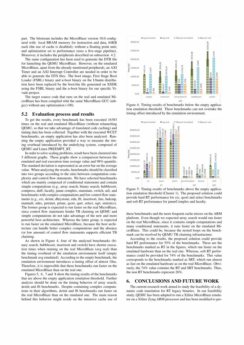
part. The bitstream includes the MicroBlaze version 10.0 config-ured with: local BRAM memory for instruction and data, 64KBeach (the use of cache is disabled); without a floating point unit;and optimization set to performance (uses a five-stage pipeline).Moreover, it includes the peripherals described on subsection 4.2.

The same configuration has been used to generate the DTB filefor launching the QEMU MicroBlaze. However, on the emulatedMicroBlaze, apart from the already mentioned peripherals, an AXITimer and an AXI Interrupt Controller are needed in order to beable to generate the DTS files. The boot image, First Stage BootLoader (FSBL) binary and u-boot binary on the Ubuntu distribu-tion have been replaced by the boot.bin file generated on XSDKusing the FSBL binary and the u-boot binary for our specific Vi-vado project.

The target source code that runs on the real and emulated Mi-croBlaze has been compiled whit the same MicroBlaze GCC (mb-gcc) without any optimization (-O0).

5.2 Evaluation process and resultsTo get the results, every benchmark has been executed 16383

times on the real and emulated MicroBlaze (without relaunchingQEMU, so that we take advantage of translated code caching) andtiming data has been collected. Together with the executed WCETbenchmarks, an empty application has also been analyzed. Run-ning the empty application provided a way to measure the tim-ing overhead introduced by the underlying system, composed ofQEMU and Linux PREEMPT_RT.

In order to solve scaling problems, result have been clustered into5 different graphs. These graphs show a comparison between theemulated and real execution time average value and 98%-quantile.The standard deviation is represented as an error bar on the averagevalue. When analyzing the results, benchmarks should be classifiedinto two groups according to the ratio between computation com-plexity and control flow statements. We have selected benchmarkswhich are mainly composed of conditional statements and containsimple computations (e.g., array search, binary search, bubblesort,compress, duff, faculty, janne complex, statemate, switch, ud), andbenchmarks with complex computations and few control flow state-ments (e.g., crc, dctint, dhrystone, edn, fft, insertsort, lms, ludcmp,matmult, ndes, petrinet, prime, qsort, qurt, select, sqrt, statistics).The former group is expected to run faster on the real MicroBlaze,since control flow statements hinder TB chaining on QEMU andsimple computations do not take advantage of the new and morepowerful host architecture. Whereas the latter group, is expectedto run faster on the emulated MicroBlaze, because the host archi-tecture can handle better complex computations and the absence(or low amount) of control flow statements supports efficient TBchaining.

As shown in Figure 4, four of the analyzed benchmarks (bi-nary search, bubblesort, insertsort and switch) have shorter execu-tion times when running on the real MicroBlaze (avg real) thanthe timing overhead of the emulation environment itself (emptybenchmark avg emulated). According to the empty benchmark, theemulation environment introduces a timing offset of almost 10us.Therefore, it is impossible that these benchmarks run faster on theemulated MicroBlaze than on the real one.

Figures 5, 6, 7 and 8 show the timing results of the benchmarksthat are above the empty application emulation threshold. Furtheranalysis should be done on the timing behavior of array search,dctint and fft benchmarks. Despite containing complex computa-tions in their algorithms, dctint and fft benchmarks run faster onthe real MicroBlaze than on the emulated one. The main reasonbehind this behavior might reside on the intensive cache use of

1087

3,95

9956

,09

1069

5,29

1455

6,88

2026

4,09

980

1144

,07

5700

3000

,08

9340

1169

7

1057

8,54

1131

9,54 15

606

2104

5

980

1140

5700

3000

9340

0,00

5000,00

10000,00

15000,00

20000,00

25000,00

30000,00

empty insertsort binarySearch bubblesort switch

NRT

Tim

e (n

s)

avg emulated avg real 98quant emulated 98quant real

Figure 4: Timing results of benchmarks below the empty applica-tion emulation threshold. These benchmarks can not overtake thetiming offset introduced by the emulation environment.

5592

3,70

2919

99,3

0

2997

29,1

1

1520

5,07

3578

0,54

1048

43,2

4

1154

47,5

2

3376

67,7

7

3702

49,5

7

1406

0

2394

0

1752

05748

9,54

3254

61,2

4

3301

13,7

1586

7,54

3840

4,86

1310

19,9

1153

40

3376

60 3704

20

1406

0

2394

0

1752

0

0,00

50000,00

100000,00

150000,00

200000,00

250000,00

300000,00

350000,00

400000,00

crc qsort select janneComplex faculty duff

RT SRT NRT

Tim

e (n

s)

avg emulated avg real 98quant emulated 98quant real

Figure 5: Timing results of benchmarks above the empty applica-tion emulation threshold (Cluster 1). The proposed solution couldprovide hard RT performance for crc, qsort and select benchmarksand soft RT performance for janneComplex and faculty.

these benchmarks and the more frequent cache misses on the ARMplatform. Even though we expected array search would run fasteron the real MicroBlaze, since it contains simple computations andmany conditional statements, it runs faster on the emulated Mi-croBlaze. This could be, because the nested loops on the bench-mark can be resolved by QEMU TB chaining infrastructure.

According to the results, the proposed solution could providehard RT performance for 55% of the benchmarks. These are thebenchmarks marked as RT in the figures, which run faster on theemulated hardware than on the real one. Whereas, soft RT perfor-mance could be provided for 74% of the benchmarks. This valuecorresponds to the benchmarks marked as SRT, which run almostas fast on the emulated hardware as on the real MicroBlaze. Obvi-ously, the 74% value contains the RT and SRT benchmarks. Thus,the non RT benchmarks represent 26%.

6. CONCLUSIONS AND FUTURE WORKThe current research work aimed to study the feasibility of a dy-

namic code translation for RT legacy binaries. In our feasibilitystudy, QEMU has been adapted to run a Xilinx MicroBlaze emula-tor on a Xilinx Zynq ARM processor and has been modified to per-

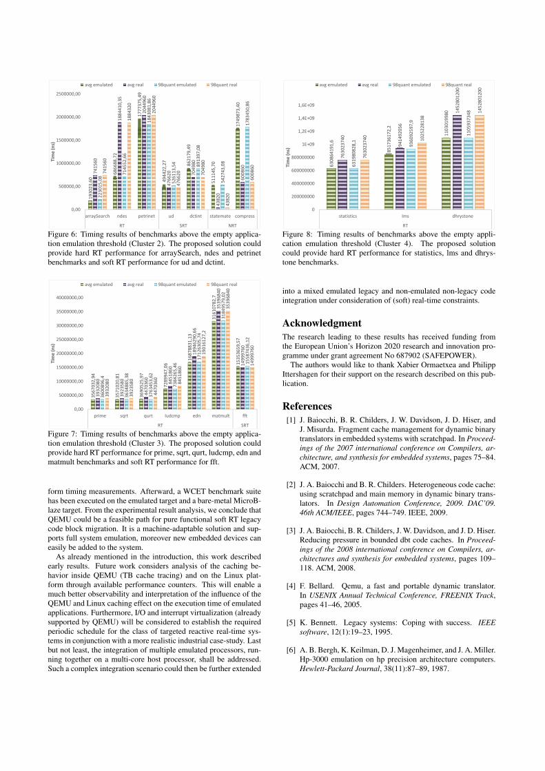
1930

23,6

0

6866

88,7

2

1777

375,

49

4944

22,2

7

8621

79,4

9

5111

45,7

0

1749

873,

40

7415

60

1884

410,

35

2044

960

4766

20 7049

80

4382

0

6008

60

2230

15,0

8

7145

52,6

6

1843

081,

86

5261

13,5

4 8913

97,0

8

5427

43,0

8

1783

450,

86

7415

60

1884

320

2044

960

4766

20 7049

80

4382

0

6008

60

0,00

500000,00

1000000,00

1500000,00

2000000,00

2500000,00

arraySearch ndes petrinet ud dctint statemate compress

RT SRT NRT

Tim

e (n

s)

avg emulated avg real 98quant emulated 98quant real

Figure 6: Timing results of benchmarks above the empty applica-tion emulation threshold (Cluster 2). The proposed solution couldprovide hard RT performance for arraySearch, ndes and petrinetbenchmarks and soft RT performance for ud and dctint.

3567

032,

94

3571

020,

81

3690

525,

97

7289

947,

06

1687

8831

,13

3161

0782

,7

1535

3659

,57

3932

080

3923

580

4470

360

8451

860

1894

6290

,66

3539

6840

1499

9760

3600

896,

4

3634

885,

38

3763

453,

62

7384

265,

46

1712

6305

,74

3184

9579

,02

1558

7436

,12

3932

080

3923

580

4470

360

8451

860

1901

6127

,2

3539

6840

1499

9760

0,00

5000000,00

10000000,00

15000000,00

20000000,00

25000000,00

30000000,00

35000000,00

40000000,00

prime sqrt qurt Iudcmp edn matmult fft

RT SRT

Tim

e (n

s)

avg emulated avg real 98quant emulated 98quant real

Figure 7: Timing results of benchmarks above the empty applica-tion emulation threshold (Cluster 3). The proposed solution couldprovide hard RT performance for prime, sqrt, qurt, ludcmp, edn andmatmult benchmarks and soft RT performance for fft.

form timing measurements. Afterward, a WCET benchmark suitehas been executed on the emulated target and a bare-metal MicroB-laze target. From the experimental result analysis, we conclude thatQEMU could be a feasible path for pure functional soft RT legacycode block migration. It is a machine-adaptable solution and sup-ports full system emulation, moreover new embedded devices caneasily be added to the system.

As already mentioned in the introduction, this work describedearly results. Future work considers analysis of the caching be-havior inside QEMU (TB cache tracing) and on the Linux plat-form through available performance counters. This will enable amuch better observability and interpretation of the influence of theQEMU and Linux caching effect on the execution time of emulatedapplications. Furthermore, I/O and interrupt virtualization (alreadysupported by QEMU) will be considered to establish the requiredperiodic schedule for the class of targeted reactive real-time sys-tems in conjunction with a more realistic industrial case-study. Lastbut not least, the integration of multiple emulated processors, run-ning together on a multi-core host processor, shall be addressed.Such a complex integration scenario could then be further extended

6308

6419

1,6

8517

3617

2,2

1103

0199

80

7630

2374

0

9414

9205

6

1452

8012

00

6319

8082

8,1

9360

9259

7,9

1105

9373

48

7630

2374

0

1025

2281

38

1452

8012

00

0

200000000

400000000

600000000

800000000

1E+09

1,2E+09

1,4E+09

1,6E+09

statistics Ims dhrystone

RT

Tim

e (n

s)

avg emulated avg real 98quant emulated 98quant real

Figure 8: Timing results of benchmarks above the empty appli-cation emulation threshold (Cluster 4). The proposed solutioncould provide hard RT performance for statistics, lms and dhrys-tone benchmarks.

into a mixed emulated legacy and non-emulated non-legacy codeintegration under consideration of (soft) real-time constraints.

AcknowledgmentThe research leading to these results has received funding fromthe European Union’s Horizon 2020 research and innovation pro-gramme under grant agreement No 687902 (SAFEPOWER).

The authors would like to thank Xabier Ormaetxea and PhilippIttershagen for their support on the research described on this pub-lication.

References[1] J. Baiocchi, B. R. Childers, J. W. Davidson, J. D. Hiser, and

J. Misurda. Fragment cache management for dynamic binarytranslators in embedded systems with scratchpad. In Proceed-ings of the 2007 international conference on Compilers, ar-chitecture, and synthesis for embedded systems, pages 75–84.ACM, 2007.

[2] J. A. Baiocchi and B. R. Childers. Heterogeneous code cache:using scratchpad and main memory in dynamic binary trans-lators. In Design Automation Conference, 2009. DAC’09.46th ACM/IEEE, pages 744–749. IEEE, 2009.

[3] J. A. Baiocchi, B. R. Childers, J. W. Davidson, and J. D. Hiser.Reducing pressure in bounded dbt code caches. In Proceed-ings of the 2008 international conference on Compilers, ar-chitectures and synthesis for embedded systems, pages 109–118. ACM, 2008.

[4] F. Bellard. Qemu, a fast and portable dynamic translator.In USENIX Annual Technical Conference, FREENIX Track,pages 41–46, 2005.

[5] K. Bennett. Legacy systems: Coping with success. IEEEsoftware, 12(1):19–23, 1995.

[6] A. B. Bergh, K. Keilman, D. J. Magenheimer, and J. A. Miller.Hp-3000 emulation on hp precision architecture computers.Hewlett-Packard Journal, 38(11):87–89, 1987.

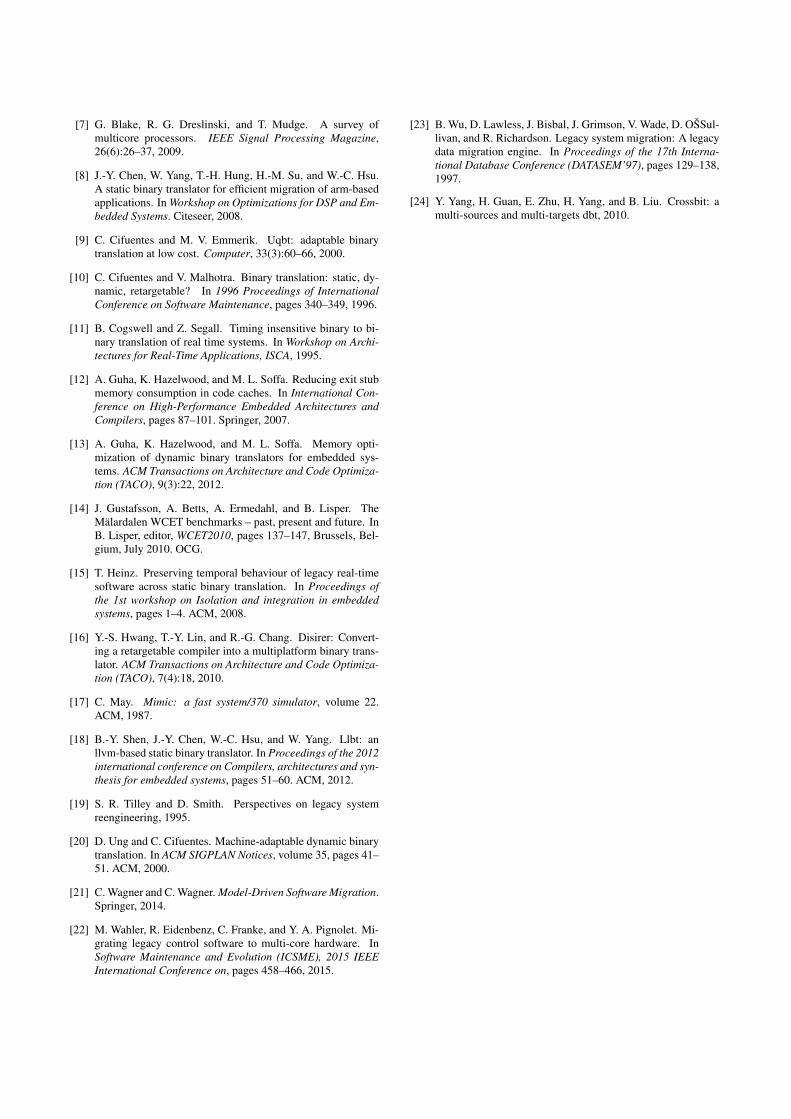
[7] G. Blake, R. G. Dreslinski, and T. Mudge. A survey ofmulticore processors. IEEE Signal Processing Magazine,26(6):26–37, 2009.

[8] J.-Y. Chen, W. Yang, T.-H. Hung, H.-M. Su, and W.-C. Hsu.A static binary translator for efficient migration of arm-basedapplications. In Workshop on Optimizations for DSP and Em-bedded Systems. Citeseer, 2008.

[9] C. Cifuentes and M. V. Emmerik. Uqbt: adaptable binarytranslation at low cost. Computer, 33(3):60–66, 2000.

[10] C. Cifuentes and V. Malhotra. Binary translation: static, dy-namic, retargetable? In 1996 Proceedings of InternationalConference on Software Maintenance, pages 340–349, 1996.

[11] B. Cogswell and Z. Segall. Timing insensitive binary to bi-nary translation of real time systems. In Workshop on Archi-tectures for Real-Time Applications, ISCA, 1995.

[12] A. Guha, K. Hazelwood, and M. L. Soffa. Reducing exit stubmemory consumption in code caches. In International Con-ference on High-Performance Embedded Architectures andCompilers, pages 87–101. Springer, 2007.

[13] A. Guha, K. Hazelwood, and M. L. Soffa. Memory opti-mization of dynamic binary translators for embedded sys-tems. ACM Transactions on Architecture and Code Optimiza-tion (TACO), 9(3):22, 2012.

[14] J. Gustafsson, A. Betts, A. Ermedahl, and B. Lisper. TheMälardalen WCET benchmarks – past, present and future. InB. Lisper, editor, WCET2010, pages 137–147, Brussels, Bel-gium, July 2010. OCG.

[15] T. Heinz. Preserving temporal behaviour of legacy real-timesoftware across static binary translation. In Proceedings ofthe 1st workshop on Isolation and integration in embeddedsystems, pages 1–4. ACM, 2008.

[16] Y.-S. Hwang, T.-Y. Lin, and R.-G. Chang. Disirer: Convert-ing a retargetable compiler into a multiplatform binary trans-lator. ACM Transactions on Architecture and Code Optimiza-tion (TACO), 7(4):18, 2010.

[17] C. May. Mimic: a fast system/370 simulator, volume 22.ACM, 1987.

[18] B.-Y. Shen, J.-Y. Chen, W.-C. Hsu, and W. Yang. Llbt: anllvm-based static binary translator. In Proceedings of the 2012international conference on Compilers, architectures and syn-thesis for embedded systems, pages 51–60. ACM, 2012.

[19] S. R. Tilley and D. Smith. Perspectives on legacy systemreengineering, 1995.

[20] D. Ung and C. Cifuentes. Machine-adaptable dynamic binarytranslation. In ACM SIGPLAN Notices, volume 35, pages 41–51. ACM, 2000.

[21] C. Wagner and C. Wagner. Model-Driven Software Migration.Springer, 2014.

[22] M. Wahler, R. Eidenbenz, C. Franke, and Y. A. Pignolet. Mi-grating legacy control software to multi-core hardware. InSoftware Maintenance and Evolution (ICSME), 2015 IEEEInternational Conference on, pages 458–466, 2015.

[23] B. Wu, D. Lawless, J. Bisbal, J. Grimson, V. Wade, D. OŠSul-livan, and R. Richardson. Legacy system migration: A legacydata migration engine. In Proceedings of the 17th Interna-tional Database Conference (DATASEM’97), pages 129–138,1997.

[24] Y. Yang, H. Guan, E. Zhu, H. Yang, and B. Liu. Crossbit: amulti-sources and multi-targets dbt, 2010.

XXXII

Design Space Pruning andComputational Workload Splittingfor Autotuning OpenCLApplications

XXXIII

Design Space Pruning and Computational WorkloadSplitting for Autotuning OpenCL Applications

Ahmet Erdem Davide Gadioli

Gianluca Palermo Cristina Silvano

Department of Electronics, Information and BioengineeringPolitecnico di Milano

e-mail: name.surname@polimi.it

ABSTRACTRecently, OpenCL standard reached much wider audiencesdue to the increasing number of devices supporting it. Atthe same time, we have observed an increase of differencesamong devices that support OpenCL. This situation offersto developers, who want to get high performance, a largespectrum of platforms. Given the additional OpenCL plat-form parameters alongside application specific parameters,the design space for exploration is seriously large. Further-more, availability of more than one kind of device allowsdistribution of computation on the heterogeneous platform.Automatic design space exploration frameworks are one ofthe recent approaches to address these problems and to re-duce the burden of programmers. In this work, we presentour automatic and efficient technique to prune the designspace before moving on to the exploration phase and wepropose a new method for splitting the computational tasksto computing devices on heterogeneous platforms.1

1. INTRODUCTIONThe recent advances in computer architecture made het-

erogeneous computer systems available to not only data cen-ters and supercomputers, but also to commercial personalcomputers. Especially, with the advent of AMD APUs andIntel CPUs which include integrated GPUs, the heterogene-ity of modern machines has increased. Furthermore, en-abling discrete GPUs for general purpose computing hasadded another type of computation device to the system.While each system has provided different granularity of par-allelism which needs to be properly exploited, the commu-nication between various computation devices must also behandled according to the requirements of application as well.

1This work is partially funded by the EU H2020 FET-HPCprogram under grant 671623 ANTAREX.

Permission to make digital or hard copies of all or part of this work for personal orclassroom use is granted without fee provided that copies are not made or distributedfor profit or commercial advantage and that copies bear this notice and the full cita-tion on the first page. Copyrights for components of this work owned by others thanACM must be honored. Abstracting with credit is permitted. To copy otherwise, or re-publish, to post on servers or to redistribute to lists, requires prior specific permissionand/or a fee. Request permissions from permissions@acm.org.

RAPIDO, January 22–24, 2018, Manchester, United Kingdomc© 2018 ACM. ISBN 978-1-4503-6417-1/18/01. . . $15.00

DOI: https://doi.org/10.1145/3180665.3180669

Open Computing Language (OpenCL), maintained by theKhronos consortium [4], is an open standard for developingparallel applications on heterogeneous systems by abstract-ing the underlying compute machine. OpenCL adopts dataparallel approach by describing the parallel computations asa group of work-items, named work-groups. In this hierar-chical mechanism, a kernel function is executed in parallelby each work-item in the work-group. A kernel function de-scribes how each work-item defines the operations carriedout on a single data. Therefore, the collection of work-itemsunder all work-groups together expresses the data paral-lelism for an application. Although OpenCL guarantees thatthe execution of the application is portable between the de-vices conforming the OpenCL standard, it does not guaran-tee the performance to be optimal. Especially, moving ap-plications to different types of architectures like from CPUto GPU may result significant loss of performance. Thisis the reason why OpenCL is not considered performanceportable. Heterogeneous platforms performance portabilityrepresents a challenging research issue.

One naive solution to performance portability is to de-velop separate kernel functions for each device the applica-tion is supposed to run. This solution makes developmentof application dramatically complicated when the system isheterogeneous, because of explicit management of multiplecommand queues and contexts in the presence of multiplevendors on the system. Moreover, this approach has moredesign flaws:

• The application developer must have knowledge of allthe device’s architectures.

• The application must be manually split between exist-ing devices on the platform.

• The developer should have access to all the devices inorder to test and profile on them.

• The number of devices targeted by the application islimited, consequently future architectures are impos-sible to target in a performance optimal way withoutmodifying the application code.

The performance portability problem of OpenCL appli-cations has been approached either by tuning significantparameters as described in [6] or by introducing Domain-specific languages to annotate kernel, to generate more spe-cialized OpenCL code[2].

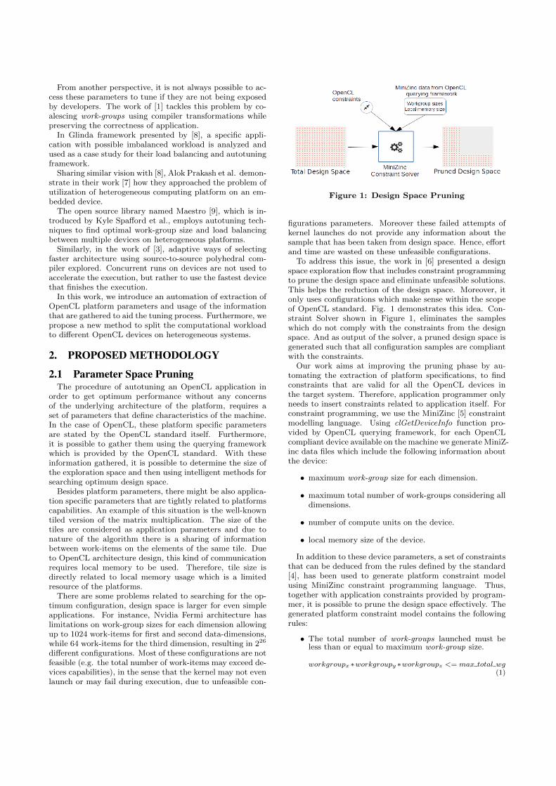
From another perspective, it is not always possible to ac-cess these parameters to tune if they are not being exposedby developers. The work of [1] tackles this problem by co-alescing work-groups using compiler transformations whilepreserving the correctness of application.

In Glinda framework presented by [8], a specific appli-cation with possible imbalanced workload is analyzed andused as a case study for their load balancing and autotuningframework.

Sharing similar vision with [8], Alok Prakash et al. demon-strate in their work [7] how they approached the problem ofutilization of heterogeneous computing platform on an em-bedded device.

The open source library named Maestro [9], which is in-troduced by Kyle Spafford et al., employs autotuning tech-niques to find optimal work-group size and load balancingbetween multiple devices on heterogeneous platforms.

Similarly, in the work of [3], adaptive ways of selectingfaster architecture using source-to-source polyhedral com-piler explored. Concurrent runs on devices are not used toaccelerate the execution, but rather to use the fastest devicethat finishes the execution.

In this work, we introduce an automation of extraction ofOpenCL platform parameters and usage of the informationthat are gathered to aid the tuning process. Furthermore, wepropose a new method to split the computational workloadto different OpenCL devices on heterogeneous systems.

2. PROPOSED METHODOLOGY

2.1 Parameter Space PruningThe procedure of autotuning an OpenCL application in

order to get optimum performance without any concernsof the underlying architecture of the platform, requires aset of parameters that define characteristics of the machine.In the case of OpenCL, these platform specific parametersare stated by the OpenCL standard itself. Furthermore,it is possible to gather them using the querying frameworkwhich is provided by the OpenCL standard. With theseinformation gathered, it is possible to determine the size ofthe exploration space and then using intelligent methods forsearching optimum design space.

Besides platform parameters, there might be also applica-tion specific parameters that are tightly related to platformscapabilities. An example of this situation is the well-knowntiled version of the matrix multiplication. The size of thetiles are considered as application parameters and due tonature of the algorithm there is a sharing of informationbetween work-items on the elements of the same tile. Dueto OpenCL architecture design, this kind of communicationrequires local memory to be used. Therefore, tile size isdirectly related to local memory usage which is a limitedresource of the platforms.

There are some problems related to searching for the op-timum configuration, design space is larger for even simpleapplications. For instance, Nvidia Fermi architecture haslimitations on work-group sizes for each dimension allowingup to 1024 work-items for first and second data-dimensions,while 64 work-items for the third dimension, resulting in 226

different configurations. Most of these configurations are notfeasible (e.g. the total number of work-items may exceed de-vices capabilities), in the sense that the kernel may not evenlaunch or may fail during execution, due to unfeasible con-

Figure 1: Design Space Pruning

figurations parameters. Moreover these failed attempts ofkernel launches do not provide any information about thesample that has been taken from design space. Hence, effortand time are wasted on these unfeasible configurations.

To address this issue, the work in [6] presented a designspace exploration flow that includes constraint programmingto prune the design space and eliminate unfeasible solutions.This helps the reduction of the design space. Moreover, itonly uses configurations which make sense within the scopeof OpenCL standard. Fig. 1 demonstrates this idea. Con-straint Solver shown in Figure 1, eliminates the sampleswhich do not comply with the constraints from the designspace. And as output of the solver, a pruned design space isgenerated such that all configuration samples are compliantwith the constraints.

Our work aims at improving the pruning phase by au-tomating the extraction of platform specifications, to findconstraints that are valid for all the OpenCL devices inthe target system. Therefore, application programmer onlyneeds to insert constraints related to application itself. Forconstraint programming, we use the MiniZinc [5] constraintmodelling language. Using clGetDeviceInfo function pro-vided by OpenCL querying framework, for each OpenCLcompliant device available on the machine we generate MiniZ-inc data files which include the following information aboutthe device:

• maximum work-group size for each dimension.

• maximum total number of work-groups considering alldimensions.

• number of compute units on the device.

• local memory size of the device.

In addition to these device parameters, a set of constraintsthat can be deduced from the rules defined by the standard[4], has been used to generate platform constraint modelusing MiniZinc constraint programming language. Thus,together with application constraints provided by program-mer, it is possible to prune the design space effectively. Thegenerated platform constraint model contains the followingrules:

• The total number of work-groups launched must beless than or equal to maximum work-group size.

workgroupx ∗workgroupy ∗workgroupz <= max total wg(1)

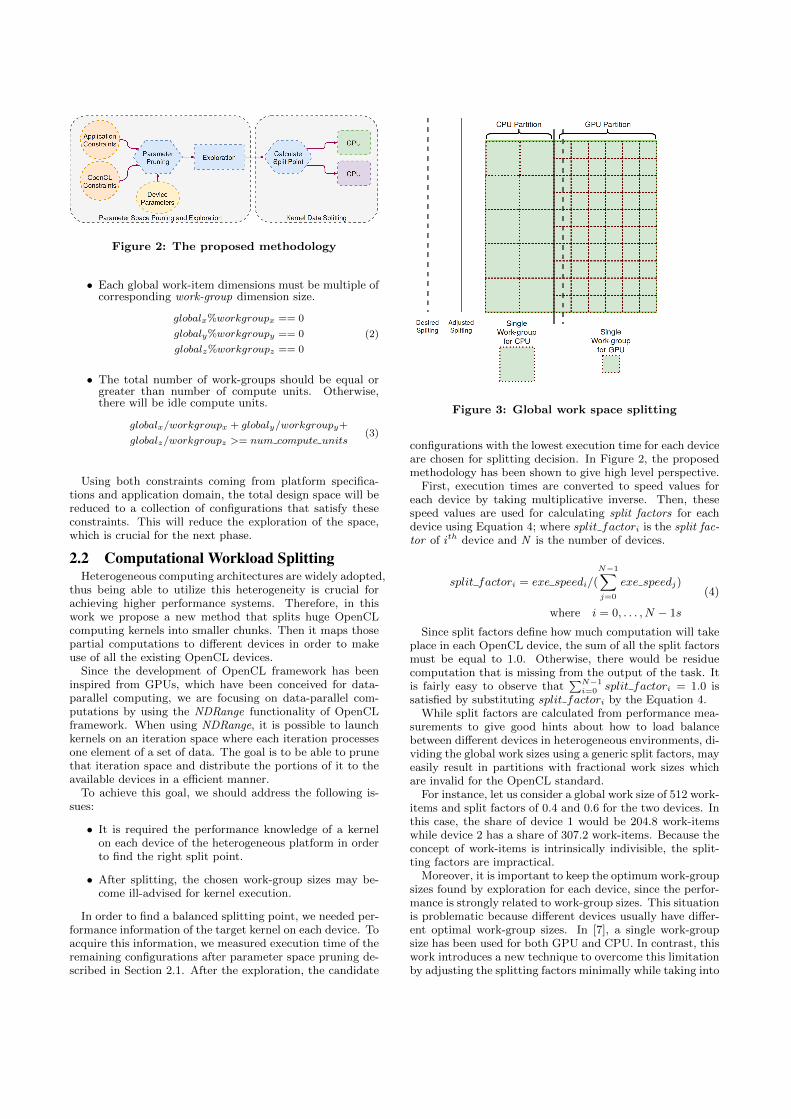
Figure 2: The proposed methodology

• Each global work-item dimensions must be multiple ofcorresponding work-group dimension size.

globalx%workgroupx == 0

globaly%workgroupy == 0

globalz%workgroupz == 0

(2)

• The total number of work-groups should be equal orgreater than number of compute units. Otherwise,there will be idle compute units.

globalx/workgroupx + globaly/workgroupy+

globalz/workgroupz >= num compute units(3)

Using both constraints coming from platform specifica-tions and application domain, the total design space will bereduced to a collection of configurations that satisfy theseconstraints. This will reduce the exploration of the space,which is crucial for the next phase.

2.2 Computational Workload SplittingHeterogeneous computing architectures are widely adopted,

thus being able to utilize this heterogeneity is crucial forachieving higher performance systems. Therefore, in thiswork we propose a new method that splits huge OpenCLcomputing kernels into smaller chunks. Then it maps thosepartial computations to different devices in order to makeuse of all the existing OpenCL devices.

Since the development of OpenCL framework has beeninspired from GPUs, which have been conceived for data-parallel computing, we are focusing on data-parallel com-putations by using the NDRange functionality of OpenCLframework. When using NDRange, it is possible to launchkernels on an iteration space where each iteration processesone element of a set of data. The goal is to be able to prunethat iteration space and distribute the portions of it to theavailable devices in a efficient manner.

To achieve this goal, we should address the following is-sues:

• It is required the performance knowledge of a kernelon each device of the heterogeneous platform in orderto find the right split point.

• After splitting, the chosen work-group sizes may be-come ill-advised for kernel execution.

In order to find a balanced splitting point, we needed per-formance information of the target kernel on each device. Toacquire this information, we measured execution time of theremaining configurations after parameter space pruning de-scribed in Section 2.1. After the exploration, the candidate

Figure 3: Global work space splitting

configurations with the lowest execution time for each deviceare chosen for splitting decision. In Figure 2, the proposedmethodology has been shown to give high level perspective.

First, execution times are converted to speed values foreach device by taking multiplicative inverse. Then, thesespeed values are used for calculating split factors for eachdevice using Equation 4; where split factori is the split fac-tor of ith device and N is the number of devices.

split factori = exe speedi/(

N−1∑

j=0

exe speedj)

where i = 0, . . . , N − 1s

(4)

Since split factors define how much computation will takeplace in each OpenCL device, the sum of all the split factorsmust be equal to 1.0. Otherwise, there would be residuecomputation that is missing from the output of the task. Itis fairly easy to observe that

∑N−1i=0 split factori = 1.0 is

satisfied by substituting split factori by the Equation 4.While split factors are calculated from performance mea-

surements to give good hints about how to load balancebetween different devices in heterogeneous environments, di-viding the global work sizes using a generic split factors, mayeasily result in partitions with fractional work sizes whichare invalid for the OpenCL standard.

For instance, let us consider a global work size of 512 work-items and split factors of 0.4 and 0.6 for the two devices. Inthis case, the share of device 1 would be 204.8 work-itemswhile device 2 has a share of 307.2 work-items. Because theconcept of work-items is intrinsically indivisible, the split-ting factors are impractical.

Moreover, it is important to keep the optimum work-groupsizes found by exploration for each device, since the perfor-mance is strongly related to work-group sizes. This situationis problematic because different devices usually have differ-ent optimal work-group sizes. In [7], a single work-groupsize has been used for both GPU and CPU. In contrast, thiswork introduces a new technique to overcome this limitationby adjusting the splitting factors minimally while taking into

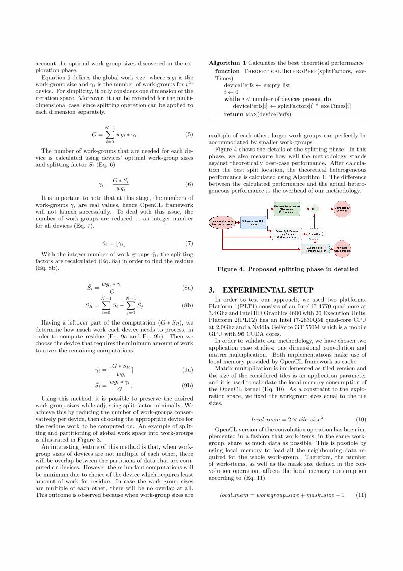
account the optimal work-group sizes discovered in the ex-ploration phase.

Equation 5 defines the global work size. where wgi is thework-group size and γi is the number of work-groups for ith

device. For simplicity, it only considers one dimension of theiteration space. Moreover, it can be extended for the multi-dimensional case, since splitting operation can be applied toeach dimension separately.

G =

N−1∑

i=0

wgi ∗ γi (5)

The number of work-groups that are needed for each de-vice is calculated using devices’ optimal work-group sizesand splitting factor Si (Eq. 6).

γi =G ∗ Si

wgi(6)

It is important to note that at this stage, the numbers ofwork-groups γi are real values, hence OpenCL frameworkwill not launch successfully. To deal with this issue, thenumber of work-groups are reduced to an integer numberfor all devices (Eq. 7).

γi = bγic (7)

With the integer number of work-groups γi, the splittingfactors are recalculated (Eq. 8a) in order to find the residue(Eq. 8b).

Si =wgi ∗ γiG

(8a)

SR =

N−1∑

i=0

Si −N−1∑

j=0

Sj (8b)

Having a leftover part of the computation (G ∗ SR), wedetermine how much work each device needs to process, inorder to compute residue (Eq. 9a and Eq. 9b). Then wechoose the device that requires the minimum amount of workto cover the remaining computations.

γi = dG ∗ SR

wgie (9a)

Si =wgi ∗ γiG

, (9b)

Using this method, it is possible to preserve the desiredwork-group sizes while adjusting split factor minimally. Weachieve this by reducing the number of work-groups conser-vatively per device, then choosing the appropriate device forthe residue work to be computed on. An example of split-ting and partitioning of global work space into work-groupsis illustrated in Figure 3.

An interesting feature of this method is that, when work-group sizes of devices are not multiple of each other, therewill be overlap between the partitions of data that are com-puted on devices. However the redundant computations willbe minimum due to choice of the device which requires leastamount of work for residue. In case the work-group sizesare multiple of each other, there will be no overlap at all.This outcome is observed because when work-group sizes are

Algorithm 1 Calculates the best theoretical performance

function TheoreticalHeteroPerf(splitFactors, exe-Times)

devicePerfs ← empty listi← 0while i < number of devices present do

devicePerfs[i] ← splitFactors[i] * exeTimes[i]

return max(devicePerfs)

multiple of each other, larger work-groups can perfectly beaccommodated by smaller work-groups.

Figure 4 shows the details of the splitting phase. In thisphase, we also measure how well the methodology standsagainst theoretically best-case performance. After calcula-tion the best split location, the theoretical heterogeneousperformance is calculated using Algorithm 1. The differencebetween the calculated performance and the actual hetero-geneous performance is the overhead of our methodology.

Figure 4: Proposed splitting phase in detailed

3. EXPERIMENTAL SETUPIn order to test our approach, we used two platforms.

Platform 1(PLT1) consists of an Intel i7-4770 quad-core at3.4Ghz and Intel HD Graphics 4600 with 20 Execution Units.Platform 2(PLT2) has an Intel i7-2630QM quad-core CPUat 2.0Ghz and a Nvidia GeForce GT 550M which is a mobileGPU with 96 CUDA cores.

In order to validate our methodology, we have chosen twoapplication case studies; one dimensional convolution andmatrix multiplication. Both implementations make use oflocal memory provided by OpenCL framework as cache.

Matrix multiplication is implemented as tiled version andthe size of the considered tiles is an application parameterand it is used to calculate the local memory consumption ofthe OpenCL kernel (Eq. 10). As a constraint to the explo-ration space, we fixed the workgroup sizes equal to the tilesizes.

local mem = 2× tile size2 (10)

OpenCL version of the convolution operation has been im-plemented in a fashion that work-items, in the same work-group, share as much data as possible. This is possible byusing local memory to load all the neighbouring data re-quired for the whole work-group. Therefore, the numberof work-items, as well as the mask size defined in the con-volution operation, affects the local memory consumptionaccording to (Eq. 11).

local mem = workgroup size+mask size− 1 (11)

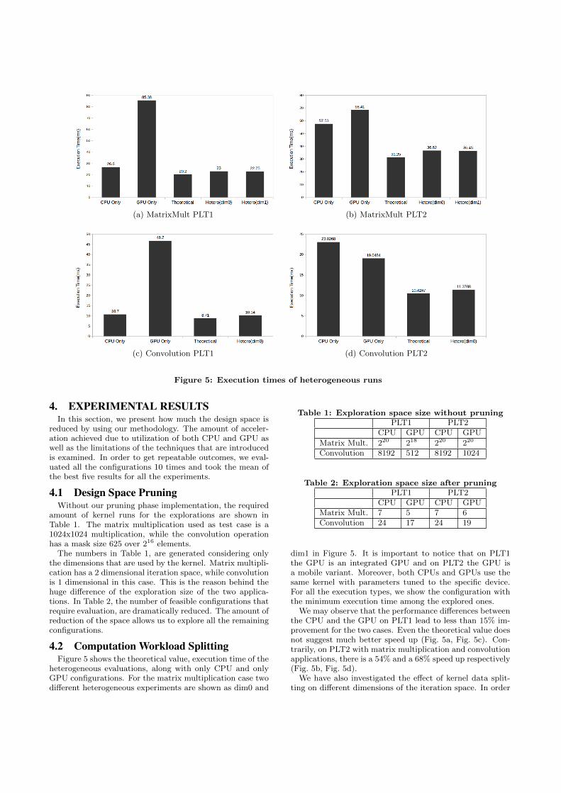
(a) MatrixMult PLT1 (b) MatrixMult PLT2

(c) Convolution PLT1 (d) Convolution PLT2

Figure 5: Execution times of heterogeneous runs

4. EXPERIMENTAL RESULTSIn this section, we present how much the design space is

reduced by using our methodology. The amount of acceler-ation achieved due to utilization of both CPU and GPU aswell as the limitations of the techniques that are introducedis examined. In order to get repeatable outcomes, we eval-uated all the configurations 10 times and took the mean ofthe best five results for all the experiments.

4.1 Design Space PruningWithout our pruning phase implementation, the required

amount of kernel runs for the explorations are shown inTable 1. The matrix multiplication used as test case is a1024x1024 multiplication, while the convolution operationhas a mask size 625 over 216 elements.

The numbers in Table 1, are generated considering onlythe dimensions that are used by the kernel. Matrix multipli-cation has a 2 dimensional iteration space, while convolutionis 1 dimensional in this case. This is the reason behind thehuge difference of the exploration size of the two applica-tions. In Table 2, the number of feasible configurations thatrequire evaluation, are dramatically reduced. The amount ofreduction of the space allows us to explore all the remainingconfigurations.

4.2 Computation Workload SplittingFigure 5 shows the theoretical value, execution time of the

heterogeneous evaluations, along with only CPU and onlyGPU configurations. For the matrix multiplication case twodifferent heterogeneous experiments are shown as dim0 and

Table 1: Exploration space size without pruningPLT1 PLT2

CPU GPU CPU GPU

Matrix Mult. 220 218 220 220

Convolution 8192 512 8192 1024

Table 2: Exploration space size after pruningPLT1 PLT2

CPU GPU CPU GPUMatrix Mult. 7 5 7 6Convolution 24 17 24 19

dim1 in Figure 5. It is important to notice that on PLT1the GPU is an integrated GPU and on PLT2 the GPU isa mobile variant. Moreover, both CPUs and GPUs use thesame kernel with parameters tuned to the specific device.For all the execution types, we show the configuration withthe minimum execution time among the explored ones.

We may observe that the performance differences betweenthe CPU and the GPU on PLT1 lead to less than 15% im-provement for the two cases. Even the theoretical value doesnot suggest much better speed up (Fig. 5a, Fig. 5c). Con-trarily, on PLT2 with matrix multiplication and convolutionapplications, there is a 54% and a 68% speed up respectively(Fig. 5b, Fig. 5d).

We have also investigated the effect of kernel data split-ting on different dimensions of the iteration space. In order

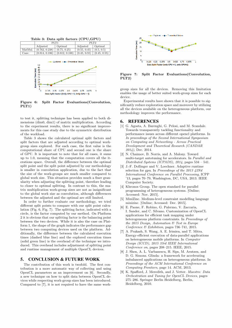
Table 3: Data split factors (CPU,GPU)PLT1 PLT2

Adjusted Optimal Adjusted OptimalMatMul. (0.762, 0.238) (0.75, 0.25) (0.55, 0.45) (0.5, 0.5)Conv. (0.814, 0.186) (0.812, 0.188) (0.45, 0.55) (0.45, 0.55)

Figure 6: Split Factor Evaluations(Convolution,PLT1)

to test it, splitting technique has been applied to both di-mensions (dim0, dim1) of matrix multiplication. Accordingto the experiment results, there is no significant improve-ments for this case study due to the symmetric distributionof the workload.

Table 3 shows the calculated optimal split factors andsplit factors that are adjusted according to optimal work-group sizes explored. For each case, the first value is thecomputational share of CPU and second one is the shareof GPU. It is important to note that for all cases, it sumsup to 1.0, meaning that the computation covers all the it-erations space. Overall, the difference between the optimalsplit point and the split point adjusted by our methodologyis smaller in convolution application, due to the fact thatthe size of the work-groups are much smaller compared toglobal work size. This situation provides much a finer gran-ularity when adjusting the splitting point, therefore leadingto closer to optimal splitting. In contrast to this, the ma-trix multiplication work-group sizes are not as insignificantto the global work size as convolution, although differencesbetween the adjusted and the optimal are still limited.

In order to further evaluate our methodology, we trieddifferent split points to compare with our split point calcu-lation (Fig. 6, Fig. 7). The splitting factor, indicated with acircle, is the factor computed by our method. On Platform2 it is obvious that our splitting factor is the balancing pointbetween the two devices. While it is also the case on Plat-form 1, the shape of the graph indicates the performance gapbetween two computing devices used on the platform. Ad-ditionally, the difference between the calculated executiontimes (dashed blue line) and the explored execution times(solid green line) is the overhead of the technique we intro-duced. This overhead includes adjustment of splitting pointand runtime management of multiple OpenCL devices.

5. CONCLUSION & FUTURE WORKThe contribution of this work is twofold. The first con-

tribution is a more automatic way of collecting and usingOpenCL parameters as an improvement on [6]. Secondly,a new technique on how to split data between OpenCL de-vices while respecting work-group sizes has been introduced.Compared to [7], it is not required to have the same work-

Figure 7: Split Factor Evaluations(Convolution,PLT2)

group sizes for all the devices. Removing this limitationenables the usage of better suited work-group sizes for eachdevice.

Experimental results have shown that it is possible to sig-nificantly reduce exploration space and moreover by utilizingall the devices available on the heterogeneous platform, ourmethodology improves the performance.

6. REFERENCES[1] G. Agosta, A. Barenghi, G. Pelosi, and M. Scandale.

Towards transparently tackling functionality andperformance issues across different opencl platforms. InIn proceedings of the Second International Symposiumon Computing and Networking - Across PracticalDevelopment and Theoretical Research (CANDAR2014), Dec. 2014.

[2] N. Chaimov, B. Norris, and A. Malony. Towardmulti-target autotuning for accelerators. In Parallel andDistributed Systems (ICPADS), 2014, pages 534 – 541.

[3] J.-F. Dollinger and V. Loechner. Adaptive runtimeselection for gpu. In Proceedings of the 2013 42NdInternational Conference on Parallel Processing, ICPP’13, pages 70–79, Washington, DC, USA, 2013. IEEEComputer Society.

[4] Khronos Group. The open standard for parallelprogramming of heterogeneous systems. [Online;Accessed: Nov. 2015].

[5] MiniZinc. Medium-level constraint modelling languageminizinc. [Online; Accessed: Dec. 2015].

[6] E. Paone, F. Robino, G. Palermo, V. Zaccaria,I. Sander, and C. Silvano. Customization of OpenCLapplications for efficient task mapping underheterogeneous platform constraints. In Proceedings ofthe 2015 Design, Automation & Test in EuropeConference & Exhibition, pages 736–741, 2015.

[7] A. Prakash, S. Wang, A. E. Irimiea, and T. Mitra.Energy-efficient execution of data-parallel applicationson heterogeneous mobile platforms. In ComputerDesign (ICCD), 2015 33rd IEEE InternationalConference on, pages 208–215. IEEE, 2015.

[8] J. Shen, A. L. Varbanescu, H. Sips, M. Arntzen, andD. G. Simons. Glinda: a framework for acceleratingimbalanced applications on heterogeneous platforms. InProceedings of the ACM International Conference onComputing Frontiers, page 14. ACM, 2013.

[9] K. Spafford, J. Meredith, and J. Vetter. Maestro: DataOrchestration and Tuning for OpenCL Devices, pages275–286. Springer Berlin Heidelberg, Berlin,Heidelberg, 2010.

XL

Compile-Time Silent StoreElimination for Energy Efficiency :an Analytic Evaluation forNon-Volatile Cache Memory

XLI

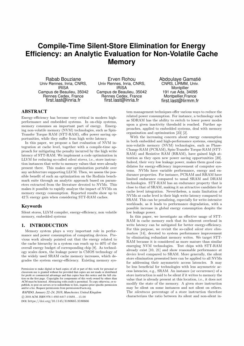
Compile-Time Silent-Store Elimination for EnergyEfficiency: an Analytic Evaluation for Non-Volatile Cache

Memory

Rabab BouzianeUniv Rennes, Inria, CNRS,

IRISACampus de Beaulieu, 35042

Rennes Cedex, Francefirst.last@inria.fr

Erven RohouUniv Rennes, Inria, CNRS,

IRISACampus de Beaulieu, 35042

Rennes Cedex, Francefirst.last@inria.fr

Abdoulaye GamatiéCNRS, LIRMM, Univ.

Montpllier191 rue Ada, 34095Montpellier,France

first.last@lirmm.fr

ABSTRACTEnergy-efficiency has become very critical in modern high-performance and embedded systems. In on-chip systems,memory consumes an important part of energy. Emerg-ing non-volatile memory (NVM) technologies, such as Spin-Transfer Torque RAM (STT-RAM), offer power saving op-portunities, while they suffer from high write latency.

In this paper, we propose a fast evaluation of NVM in-tegration at cache level, together with a compile-time ap-proach for mitigating the penalty incurred by the high writelatency of STT-RAM. We implement a code optimization inLLVM for reducing so-called silent stores, i.e., store instruc-tion instances that write to memory values that were alreadypresent there. This makes our optimization portable overany architecture supporting LLVM. Then, we assess the pos-sible benefit of such an optimization on the Rodinia bench-mark suite through an analytic approach based on param-eters extracted from the literature devoted to NVMs. Thismakes it possible to rapidly analyze the impact of NVMs onmemory energy consumption. Reported results show up to42 % energy gain when considering STT-RAM caches.

KeywordsSilent stores, LLVM compiler, energy-efficiency, non volatilememory, embedded systems

1. INTRODUCTIONMemory system plays a very important role in perfor-

mance and power consumption of computing devices. Pre-vious work already pointed out that the energy related tothe cache hierarchy in a system can reach up to 40% of theoverall energy budget of corresponding chip [8]. As technol-ogy scales down, the leakage power in CMOS technology ofthe widely used SRAM cache memory increases, which de-grades the system energy-efficiency. Existing memory sys-

Permission to make digital or hard copies of all or part of this work for personal orclassroom use is granted without fee provided that copies are not made or distributedfor profit or commercial advantage and that copies bear this notice and the full cita-tion on the first page. Copyrights for components of this work owned by others thanACM must be honored. Abstracting with credit is permitted. To copy otherwise, or re-publish, to post on servers or to redistribute to lists, requires prior specific permissionand/or a fee. Request permissions from permissions@acm.org.

RAPIDO, January 22–24, 2018, Manchester, United Kingdomc© 2018 ACM. ISBN 978-1-4503-6417-1/18/01. . .15.00

DOI: https://doi.org/10.1145/3180665.3180666

tem management techniques offer various ways to reduce therelated power consumption. For instance, a technology suchas SDRAM has the ability to switch to lower power modesupon a given inactivity threshold is reached. Further ap-proaches, applied to embedded systems, deal with memoryorganization and optimization [23] [2].

With the increasing concern about energy consumptionin both embedded and high-performance systems, emergingnon-volatile memory (NVM) technologies, such as Phase-Change RAM (PCRAM), Spin-Transfer Torque RAM (STT-RAM) and Resistive RAM (RRAM), have gained high at-tention as they open new power saving opportunities [20].Indeed, their very low leakage power, makes them good can-didates for energy-efficiency improvement of computer sys-tems. NVMs have variable performance, energy and en-durance properties. For instance, PCRAM and RRAM havelimited endurance compared to usual SRAM and DRAMtechnologies. STT-RAM has an endurance property that isclose to that of SRAM, making it an attractive candidate forcache level integration. Nevertheless, a main limitation ofNVMs at cache level is their high write latency compared toSRAM. This can be penalizing, especially for write-intensiveworkloads, as it leads to performance degradation, with apossible increase in global energy consumption despite thelow leakage power.

In this paper, we investigate an effective usage of STT-RAM in cache memory such that its inherent overhead inwrite latency can be mitigated for better energy-efficiency.For this purpose, we revisit the so-called silent store elim-ination [14], devoted to system performance improvementby eliminating redundant memory writes. We target STT-RAM because it is considered as more mature than similaremerging NVM technologies. Test chips with STT-RAMalready exist [10, 21] and show reasonable performance atdevice level compared to SRAM. More generally, the silentstore elimination presented here can be applied to all NVMsfor addressing their asymmetric access latencies. It maybe less beneficial for technologies with less asymmetric ac-cess latencies, e.g., SRAM. An instance (or occurrence) of astore instruction is said to be silent if it writes to memory thevalue that is already present at this location, i.e., it does notmodify the state of the memory. A given store instructionmay be silent on some instances and not silent on others.The silentness percentage of a store instruction thereforecharacterizes the ratio between its silent and non-silent in-

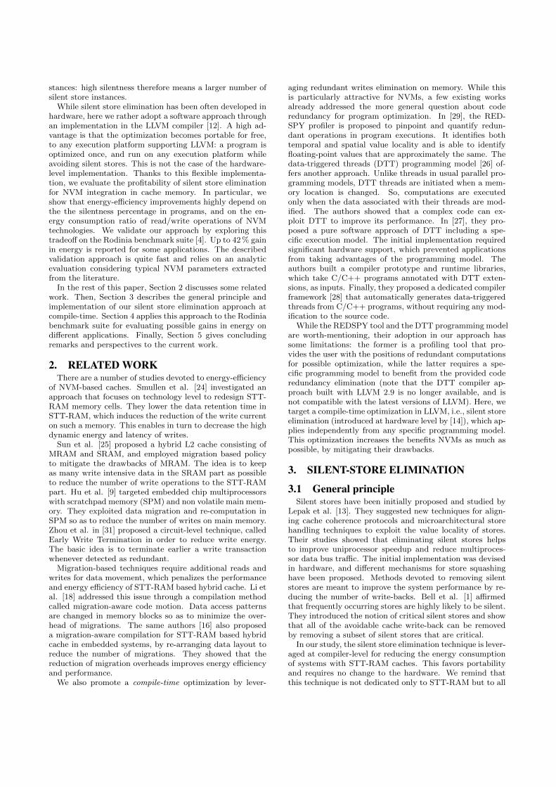
stances: high silentness therefore means a larger number ofsilent store instances.

While silent store elimination has been often developed inhardware, here we rather adopt a software approach throughan implementation in the LLVM compiler [12]. A high ad-vantage is that the optimization becomes portable for free,to any execution platform supporting LLVM: a program isoptimized once, and run on any execution platform whileavoiding silent stores. This is not the case of the hardware-level implementation. Thanks to this flexible implementa-tion, we evaluate the profitability of silent store eliminationfor NVM integration in cache memory. In particular, weshow that energy-efficiency improvements highly depend onthe the silentness percentage in programs, and on the en-ergy consumption ratio of read/write operations of NVMtechnologies. We validate our approach by exploring thistradeoff on the Rodinia benchmark suite [4]. Up to 42 % gainin energy is reported for some applications. The describedvalidation approach is quite fast and relies on an analyticevaluation considering typical NVM parameters extractedfrom the literature.

In the rest of this paper, Section 2 discusses some relatedwork. Then, Section 3 describes the general principle andimplementation of our silent store elimination approach atcompile-time. Section 4 applies this approach to the Rodiniabenchmark suite for evaluating possible gains in energy ondifferent applications. Finally, Section 5 gives concludingremarks and perspectives to the current work.

2. RELATED WORKThere are a number of studies devoted to energy-efficiency

of NVM-based caches. Smullen et al. [24] investigated anapproach that focuses on technology level to redesign STT-RAM memory cells. They lower the data retention time inSTT-RAM, which induces the reduction of the write currenton such a memory. This enables in turn to decrease the highdynamic energy and latency of writes.

Sun et al. [25] proposed a hybrid L2 cache consisting ofMRAM and SRAM, and employed migration based policyto mitigate the drawbacks of MRAM. The idea is to keepas many write intensive data in the SRAM part as possibleto reduce the number of write operations to the STT-RAMpart. Hu et al. [9] targeted embedded chip multiprocessorswith scratchpad memory (SPM) and non volatile main mem-ory. They exploited data migration and re-computation inSPM so as to reduce the number of writes on main memory.Zhou et al. in [31] proposed a circuit-level technique, calledEarly Write Termination in order to reduce write energy.The basic idea is to terminate earlier a write transactionwhenever detected as redundant.

Migration-based techniques require additional reads andwrites for data movement, which penalizes the performanceand energy efficiency of STT-RAM based hybrid cache. Li etal. [18] addressed this issue through a compilation methodcalled migration-aware code motion. Data access patternsare changed in memory blocks so as to minimize the over-head of migrations. The same authors [16] also proposeda migration-aware compilation for STT-RAM based hybridcache in embedded systems, by re-arranging data layout toreduce the number of migrations. They showed that thereduction of migration overheads improves energy efficiencyand performance.

We also promote a compile-time optimization by lever-

aging redundant writes elimination on memory. While thisis particularly attractive for NVMs, a few existing worksalready addressed the more general question about coderedundancy for program optimization. In [29], the RED-SPY profiler is proposed to pinpoint and quantify redun-dant operations in program executions. It identifies bothtemporal and spatial value locality and is able to identifyfloating-point values that are approximately the same. Thedata-triggered threads (DTT) programming model [26] of-fers another approach. Unlike threads in usual parallel pro-gramming models, DTT threads are initiated when a mem-ory location is changed. So, computations are executedonly when the data associated with their threads are mod-ified. The authors showed that a complex code can ex-ploit DTT to improve its performance. In [27], they pro-posed a pure software approach of DTT including a spe-cific execution model. The initial implementation requiredsignificant hardware support, which prevented applicationsfrom taking advantages of the programming model. Theauthors built a compiler prototype and runtime libraries,which take C/C++ programs annotated with DTT exten-sions, as inputs. Finally, they proposed a dedicated compilerframework [28] that automatically generates data-triggeredthreads from C/C++ programs, without requiring any mod-ification to the source code.

While the REDSPY tool and the DTT programming modelare worth-mentioning, their adoption in our approach hassome limitations: the former is a profiling tool that pro-vides the user with the positions of redundant computationsfor possible optimization, while the latter requires a spe-cific programming model to benefit from the provided coderedundancy elimination (note that the DTT compiler ap-proach built with LLVM 2.9 is no longer available, and isnot compatible with the latest versions of LLVM). Here, wetarget a compile-time optimization in LLVM, i.e., silent storeelimination (introduced at hardware level by [14]), which ap-plies independently from any specific programming model.This optimization increases the benefits NVMs as much aspossible, by mitigating their drawbacks.

3. SILENT-STORE ELIMINATION

3.1 General principleSilent stores have been initially proposed and studied by

Lepak et al. [13]. They suggested new techniques for align-ing cache coherence protocols and microarchitectural storehandling techniques to exploit the value locality of stores.Their studies showed that eliminating silent stores helpsto improve uniprocessor speedup and reduce multiproces-sor data bus traffic. The initial implementation was devisedin hardware, and different mechanisms for store squashinghave been proposed. Methods devoted to removing silentstores are meant to improve the system performance by re-ducing the number of write-backs. Bell et al. [1] affirmedthat frequently occurring stores are highly likely to be silent.They introduced the notion of critical silent stores and showthat all of the avoidable cache write-back can be removedby removing a subset of silent stores that are critical.

In our study, the silent store elimination technique is lever-aged at compiler-level for reducing the energy consumptionof systems with STT-RAM caches. This favors portabilityand requires no change to the hardware. We remind thatthis technique is not dedicated only to STT-RAM but to all

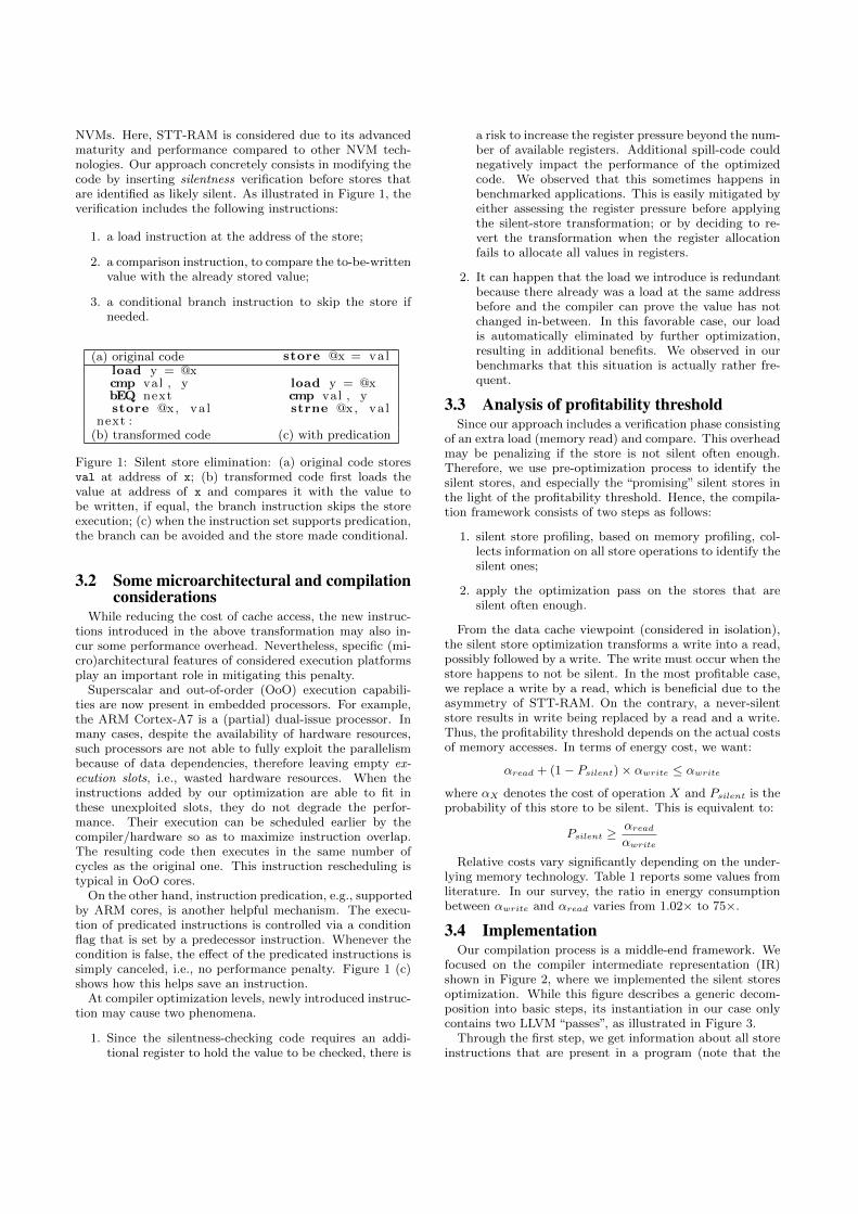
NVMs. Here, STT-RAM is considered due to its advancedmaturity and performance compared to other NVM tech-nologies. Our approach concretely consists in modifying thecode by inserting silentness verification before stores thatare identified as likely silent. As illustrated in Figure 1, theverification includes the following instructions:

1. a load instruction at the address of the store;

2. a comparison instruction, to compare the to-be-writtenvalue with the already stored value;

3. a conditional branch instruction to skip the store ifneeded.

(a) original code store @x = valload y = @xcmp val , ybEQ nextstore @x, va l

next :

load y = @xcmp val , ystrne @x, va l

(b) transformed code (c) with predication

Figure 1: Silent store elimination: (a) original code storesval at address of x; (b) transformed code first loads thevalue at address of x and compares it with the value tobe written, if equal, the branch instruction skips the storeexecution; (c) when the instruction set supports predication,the branch can be avoided and the store made conditional.

3.2 Some microarchitectural and compilationconsiderations

While reducing the cost of cache access, the new instruc-tions introduced in the above transformation may also in-cur some performance overhead. Nevertheless, specific (mi-cro)architectural features of considered execution platformsplay an important role in mitigating this penalty.

Superscalar and out-of-order (OoO) execution capabili-ties are now present in embedded processors. For example,the ARM Cortex-A7 is a (partial) dual-issue processor. Inmany cases, despite the availability of hardware resources,such processors are not able to fully exploit the parallelismbecause of data dependencies, therefore leaving empty ex-ecution slots, i.e., wasted hardware resources. When theinstructions added by our optimization are able to fit inthese unexploited slots, they do not degrade the perfor-mance. Their execution can be scheduled earlier by thecompiler/hardware so as to maximize instruction overlap.The resulting code then executes in the same number ofcycles as the original one. This instruction rescheduling istypical in OoO cores.

On the other hand, instruction predication, e.g., supportedby ARM cores, is another helpful mechanism. The execu-tion of predicated instructions is controlled via a conditionflag that is set by a predecessor instruction. Whenever thecondition is false, the effect of the predicated instructions issimply canceled, i.e., no performance penalty. Figure 1 (c)shows how this helps save an instruction.

At compiler optimization levels, newly introduced instruc-tion may cause two phenomena.

1. Since the silentness-checking code requires an addi-tional register to hold the value to be checked, there is

a risk to increase the register pressure beyond the num-ber of available registers. Additional spill-code couldnegatively impact the performance of the optimizedcode. We observed that this sometimes happens inbenchmarked applications. This is easily mitigated byeither assessing the register pressure before applyingthe silent-store transformation; or by deciding to re-vert the transformation when the register allocationfails to allocate all values in registers.

2. It can happen that the load we introduce is redundantbecause there already was a load at the same addressbefore and the compiler can prove the value has notchanged in-between. In this favorable case, our loadis automatically eliminated by further optimization,resulting in additional benefits. We observed in ourbenchmarks that this situation is actually rather fre-quent.

3.3 Analysis of profitability thresholdSince our approach includes a verification phase consisting

of an extra load (memory read) and compare. This overheadmay be penalizing if the store is not silent often enough.Therefore, we use pre-optimization process to identify thesilent stores, and especially the “promising” silent stores inthe light of the profitability threshold. Hence, the compila-tion framework consists of two steps as follows:

1. silent store profiling, based on memory profiling, col-lects information on all store operations to identify thesilent ones;

2. apply the optimization pass on the stores that aresilent often enough.

From the data cache viewpoint (considered in isolation),the silent store optimization transforms a write into a read,possibly followed by a write. The write must occur when thestore happens to not be silent. In the most profitable case,we replace a write by a read, which is beneficial due to theasymmetry of STT-RAM. On the contrary, a never-silentstore results in write being replaced by a read and a write.Thus, the profitability threshold depends on the actual costsof memory accesses. In terms of energy cost, we want:

αread + (1− Psilent)× αwrite ≤ αwritewhere αX denotes the cost of operation X and Psilent is theprobability of this store to be silent. This is equivalent to:

Psilent ≥ αreadαwrite

Relative costs vary significantly depending on the under-lying memory technology. Table 1 reports some values fromliterature. In our survey, the ratio in energy consumptionbetween αwrite and αread varies from 1.02× to 75×.

3.4 ImplementationOur compilation process is a middle-end framework. We

focused on the compiler intermediate representation (IR)shown in Figure 2, where we implemented the silent storesoptimization. While this figure describes a generic decom-position into basic steps, its instantiation in our case onlycontains two LLVM “passes”, as illustrated in Figure 3.

Through the first step, we get information about all storeinstructions that are present in a program (note that the

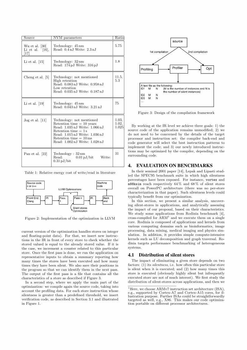
Source NVM parameters Ratio

Wu et al. [30]Li et al. [16],[17]

Technology: 45 nmRead: 0.4 nJ Write: 2.3 nJ

5.75

Li et al. [15] Technology: 32 nmRead: 174 pJ Write: 316 pJ

1.8

Cheng et al. [5] Technology: not mentionedHigh retentionRead: 0.083 nJ Write: 0.958 nJLow retentionRead: 0.035 nJ Write: 0.187 nJ

11.5,5.3

Li et al. [19] Technology: 45 nmRead: 0.043 nJ Write: 3.21 nJ

75

Jog et al. [11] Technology: not mentionedRetention time = 10 yearsRead: 1.035 nJ Write: 1.066 nJRetention time = 1 sRead: 1.015 nJ Write: 1.036 nJRetention time = 10 msRead: 1.002 nJ Write: 1.028 nJ

1.03,1.02,1.025

Pan et al. [22] Technology : 32 nmRead: 0.01 pJ/bit Write:0.31 pJ/bit

31

Table 1: Relative energy cost of write/read in literature

Figure 2: Implementation of the optimization in LLVM

current version of the optimization handles stores on integerand floating-point data). For that, we insert new instruc-tions in the IR in front of every store to check whether thestored valued is equal to the already stored value. If it isthe case, we increment a counter related to this particularstore. Once the first pass is done, we run the application onrepresentative inputs to obtain a summary reporting howmany times the stores have been executed and how manytimes they have been silent. We also save their positions inthe program so that we can identify them in the next pass.The output of the first pass is a file that contains all thecharacteristics of a store as described if Figure 3.

In a second step, where we apply the main part of theoptimization: we compile again the source code, taking intoaccount the profiling data. For each store instruction whosesilentness is greater than a predefined threshold, we insertverification code, as described in Section 3.1 and illustratedin Figure 1.

Figure 3: Design of the compilation framework

By working at the IR level we achieve three goals: 1) thesource code of the application remains unmodified; 2) wedo not need to be concerned by the details of the targetprocessor and instruction set: the compiler back-end andcode generator will select the best instruction patterns toimplement the code; and 3) our newly introduced instruc-tions may be optimized by the compiler, depending on thesurrounding code.

4. EVALUATION ON BENCHMARKSIn their seminal 2001 paper [14], Lepak and Lipasti stud-

ied the SPEC95 benchmark suite in which high silentnesspercentages have been exposed. For instance, vortex andm88ksim reach respectively 64 % and 68 % of silent storesoverall on PowerPC architecture (there was no per-storecharacterization in that paper). Such silentness levels couldtypically benefit from our optimization.

In this section, we present a similar analysis, uncover-ing silent-stores in applications, and analytically assessingthe impact of our proposal, based on their characteristics.We study some applications from Rodinia benchmark [4],cross-compiled for ARM1 and we execute them on a singlecore. Rodinia is composed of applications and kernels fromvarious computing domains such as bioinformatics, imageprocessing, data mining, medical imaging and physics sim-ulation. In addition, it provides simple compute-intensivekernels such as LU decomposition and graph traversal. Ro-dinia targets performance benchmarking of heterogeneoussystems.

4.1 Distribution of silent storesThe impact of eliminating a given store depends on two

factors: (1) its silentness, i.e. how often this particular storeis silent when it is executed; and (2) how many times thisstore is executed (obviously highly silent but infrequentlyexecuted store are not of much interest). We first study thedistribution of silent-stores across applications, and then we

1Here, we choose ARMv7 instruction set architecture (ISA),e.g., supported by Cortex-A7 and Cortex-A15 cores, for il-lustration purpose. Further ISAs could be straightforwardlytargeted as well, e.g., X86. This makes our code optimiza-tion portable on different processor architectures.

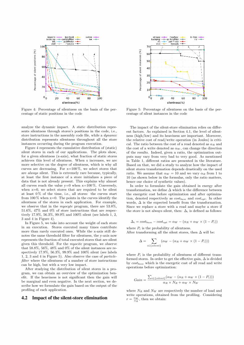
Perc

enta

ge o

f si

lent

pos

ition

s (%

)

Figure 4: Percentage of silentness on the basis of the per-centage of static positions in the code

analyze the dynamic impact. A static distribution repre-sents silentness through stores’s positions in the code, i.e.,store instructions in the assembly code file, while a dynamicdistribution represents silentness throughout all the storeinstances occurring during the program execution.

Figure 4 represents the cumulative distribution of (static)silent stores in each of our applications. The plots show,for a given silentness (x-axis), what fraction of static storesachieves this level of silentness. When x increases, we aremore selective on the degree of silentness, which is why allcurves are decreasing. For x=100 %, we select stores thatare always silent. This is extremely rare because, typically,at least the first instance of a store initializes a piece ofdata that is not already present. This explains why almostall curves reach the value y=0 when x=100 %. Conversely,when x=0, we select stores that are required to be silentat least 0 % of the time, i.e., all stores: the curves startfrom 100 % when x=0. The points in the curves identify thesilentness of the stores in each application. For example,we observe that in the myocyte program, there are 53.8%,51.6%, 47% and 0% of store instructions that are respec-tively 17.9%, 56.3%, 99.9% and 100% silent (see labels 1, 2,3 and 4 in Figure 4).

In Figure 5, we take into account the weight of each storein an execution. Stores executed many times contributemore than rarely executed ones. While the x-axis still de-notes the same threshold filter for silentness, the y-axis nowrepresents the fraction of total executed stores that are silentgiven this threshold. For the myocite program, we observethat 58.8%, 56%, 48% and 0% of the silent instances are re-spectively 17.9%, 56.3%, 99.9% and 100% silent (see labels1, 2, 3 and 4 in Figure 5). Also observe the case of particle-filter where the silentness of a number of store instructionscan be high, but with a very low impact.

After studying the distribution of silent stores in a pro-gram, we can obtain an overview of the optimization ben-efit. If the heaviness is not significant then the gain willbe marginal and even negative. In the next section, we de-scribe how we formulate the gain based on the output of theprofiling of each application.

4.2 Impact of the silent-store elimination

kmeansbackprop

heartwallX— particlefilter — ©

pathfindersrad -B— myocyte A

b+treetnw — v

bfs

70 1x x— K

60

50

40

30«

20

6810

© e0 0 20 40 60 80 100silentness klllllll(%)

Perc

enta

ge o

f si

lent

inst

ance

s (%

)

Figure 5: Percentage of silentness on the basis of the per-centage of silent instances in the code

The impact of the silent-store elimination relies on differ-ent factors. As explained in Section 4.1, the level of silent-ness (high/low) and its heaviness are important. Moreover,the relative cost of read/write operation (in Joules) is criti-cal. The ratio between the cost of a read denoted as αR andthe cost of a write denoted as αW , can change the directionof the results. Indeed, given a ratio, the optimization out-puts may vary from very bad to very good. As mentionedin Table 1, different ratios are presented in the literature.Based on that, we did a study to analyze how the impact ofsilent stores transformation depends drastically on the usedratio. We assume that αW = 10 and we vary αR from 1 to10 (as shown below in the formulas, only the ratio matters,hence our choice of synthetic values).

In order to formulate the gain obtained in energy aftertransformation, we define ∆ which is the difference betweenthe energetic cost before optimization and after optimiza-tion, denoted respectively as costbase and costopt. In otherwords, ∆ is the expected benefit from the transformation.Since we replace a store with a read and maybe a store ifthe store is not always silent, then: ∆i is defined as follows:

∆i = costbase − costopt = αW − (αR + αW × (1− Pi))where Pi is the probability of silentness.After transforming all the silent stores, then ∆ will be:

∆ =∑

i∈{silent}(αW − (αR + αW × (1− Pi)))

where Pi is the probability of silentness of different trans-formed stores. In order to get the effective gain, ∆ is dividedby costbase which is the energetic cost of all read and writeoperations before optimization:

Gain =

∑i∈{silent}(αW − (αR + αW × (1− Pi)))

αR ×NR + αW ×NW

where NR and NW are respectively the number of load andwrite operations, obtained from the profiling. Consideringr = αW

αR, then we obtain:

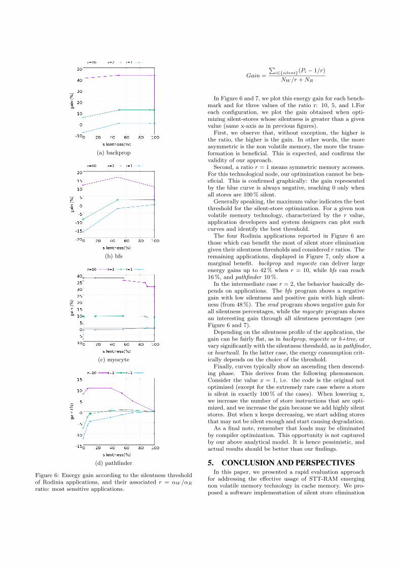
(a) backprop

(b) bfs

(c) myocyte

(d) pathfinder

Figure 6: Energy gain according to the silentness thresholdof Rodinia applications, and their associated r = αW /αRratio: most sensitive applications.

Gain =

∑i∈{silent}(Pi − 1/r)

NW /r +NR

In Figure 6 and 7, we plot this energy gain for each bench-mark and for three values of the ratio r: 10, 5, and 1.Foreach configuration, we plot the gain obtained when opti-mizing silent-stores whose silentness is greater than a givenvalue (same x-axis as in previous figures).

First, we observe that, without exception, the higher isthe ratio, the higher is the gain. In other words, the moreasymmetric is the non volatile memory, the more the trans-formation is beneficial. This is expected, and confirms thevalidity of our approach.

Second, a ratio r = 1 means symmetric memory accesses.For this technological node, our optimization cannot be ben-eficial. This is confirmed graphically: the gain representedby the blue curve is always negative, reaching 0 only whenall stores are 100 % silent.

Generally speaking, the maximum value indicates the bestthreshold for the silent-store optimization. For a given nonvolatile memory technology, characterized by the r value,application developers and system designers can plot suchcurves and identify the best threshold.

The four Rodinia applications reported in Figure 6 arethose which can benefit the most of silent store eliminationgiven their silentness thresholds and considered r ratios. Theremaining applications, displayed in Figure 7, only show amarginal benefit. backprop and myocite can deliver largeenergy gains up to 42 % when r = 10, while bfs can reach16 %, and pathfinder 10 %.

In the intermediate case r = 2, the behavior basically de-pends on applications. The bfs program shows a negativegain with low silentness and positive gain with high silent-ness (from 48 %). The srad program shows negative gain forall silentness percentages, while the myocyte program showsan interesting gain through all silentness percentages (seeFigure 6 and 7).

Depending on the silentness profile of the application, thegain can be fairly flat, as in backprop, myocite or b+tree, orvary significantly with the silentness threshold, as in pathfinder,or heartwall. In the latter case, the energy consumption crit-ically depends on the choice of the threshold.

Finally, curves typically show an ascending then descend-ing phase. This derives from the following phenomenon.Consider the value x = 1, i.e. the code is the original notoptimized (except for the extremely rare case where a storeis silent in exactly 100 % of the cases). When lowering x,we increase the number of store instructions that are opti-mized, and we increase the gain because we add highly silentstores. But when x keeps decreasing, we start adding storesthat may not be silent enough and start causing degradation.

As a final note, remember that loads may be eliminatedby compiler optimization. This opportunity is not capturedby our above analytical model. It is hence pessimistic, andactual results should be better than our findings.

5. CONCLUSION AND PERSPECTIVESIn this paper, we presented a rapid evaluation approach

for addressing the effective usage of STT-RAM emergingnon volatile memory technology in cache memory. We pro-posed a software implementation of silent store elimination

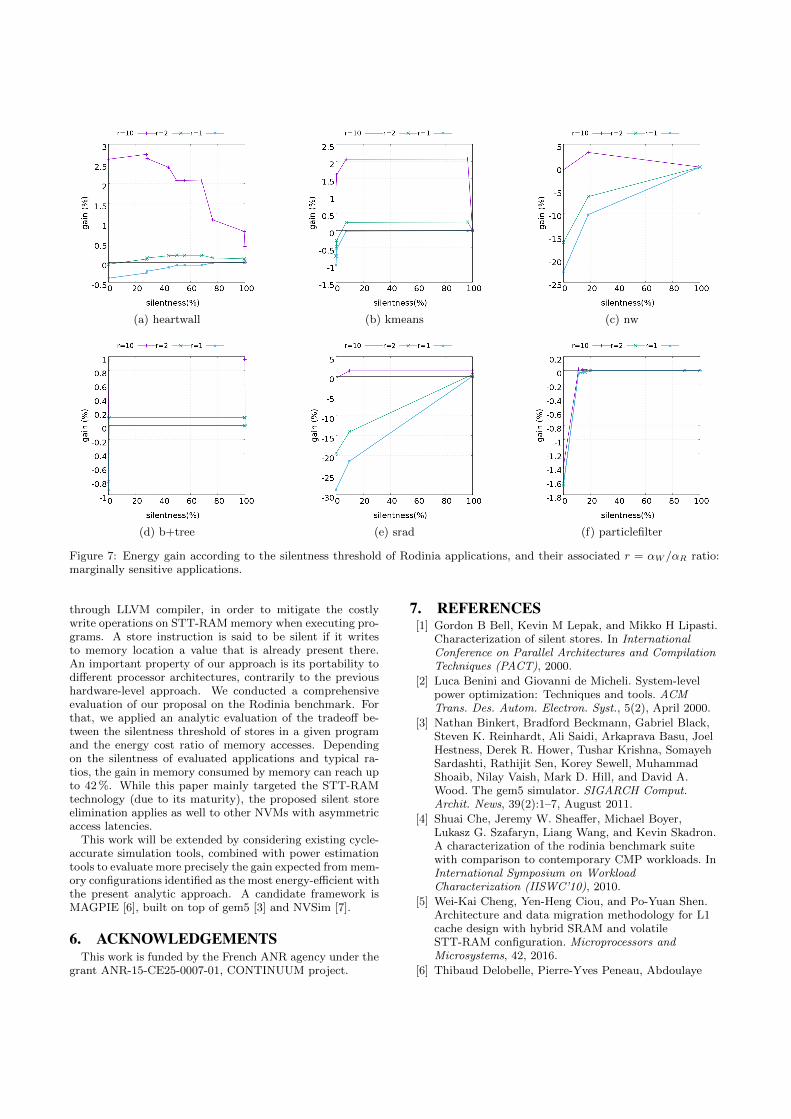
(a) heartwall (b) kmeans (c) nw

(d) b+tree (e) srad (f) particlefilter

Figure 7: Energy gain according to the silentness threshold of Rodinia applications, and their associated r = αW /αR ratio:marginally sensitive applications.

through LLVM compiler, in order to mitigate the costlywrite operations on STT-RAM memory when executing pro-grams. A store instruction is said to be silent if it writesto memory location a value that is already present there.An important property of our approach is its portability todifferent processor architectures, contrarily to the previoushardware-level approach. We conducted a comprehensiveevaluation of our proposal on the Rodinia benchmark. Forthat, we applied an analytic evaluation of the tradeoff be-tween the silentness threshold of stores in a given programand the energy cost ratio of memory accesses. Dependingon the silentness of evaluated applications and typical ra-tios, the gain in memory consumed by memory can reach upto 42 %. While this paper mainly targeted the STT-RAMtechnology (due to its maturity), the proposed silent storeelimination applies as well to other NVMs with asymmetricaccess latencies.

This work will be extended by considering existing cycle-accurate simulation tools, combined with power estimationtools to evaluate more precisely the gain expected from mem-ory configurations identified as the most energy-efficient withthe present analytic approach. A candidate framework isMAGPIE [6], built on top of gem5 [3] and NVSim [7].

6. ACKNOWLEDGEMENTSThis work is funded by the French ANR agency under the

grant ANR-15-CE25-0007-01, CONTINUUM project.

7. REFERENCES[1] Gordon B Bell, Kevin M Lepak, and Mikko H Lipasti.

Characterization of silent stores. In InternationalConference on Parallel Architectures and CompilationTechniques (PACT), 2000.

[2] Luca Benini and Giovanni de Micheli. System-levelpower optimization: Techniques and tools. ACMTrans. Des. Autom. Electron. Syst., 5(2), April 2000.

[3] Nathan Binkert, Bradford Beckmann, Gabriel Black,Steven K. Reinhardt, Ali Saidi, Arkaprava Basu, JoelHestness, Derek R. Hower, Tushar Krishna, SomayehSardashti, Rathijit Sen, Korey Sewell, MuhammadShoaib, Nilay Vaish, Mark D. Hill, and David A.Wood. The gem5 simulator. SIGARCH Comput.Archit. News, 39(2):1–7, August 2011.

[4] Shuai Che, Jeremy W. Sheaffer, Michael Boyer,Lukasz G. Szafaryn, Liang Wang, and Kevin Skadron.A characterization of the rodinia benchmark suitewith comparison to contemporary CMP workloads. InInternational Symposium on WorkloadCharacterization (IISWC’10), 2010.

[5] Wei-Kai Cheng, Yen-Heng Ciou, and Po-Yuan Shen.Architecture and data migration methodology for L1cache design with hybrid SRAM and volatileSTT-RAM configuration. Microprocessors andMicrosystems, 42, 2016.

[6] Thibaud Delobelle, Pierre-Yves Peneau, Abdoulaye

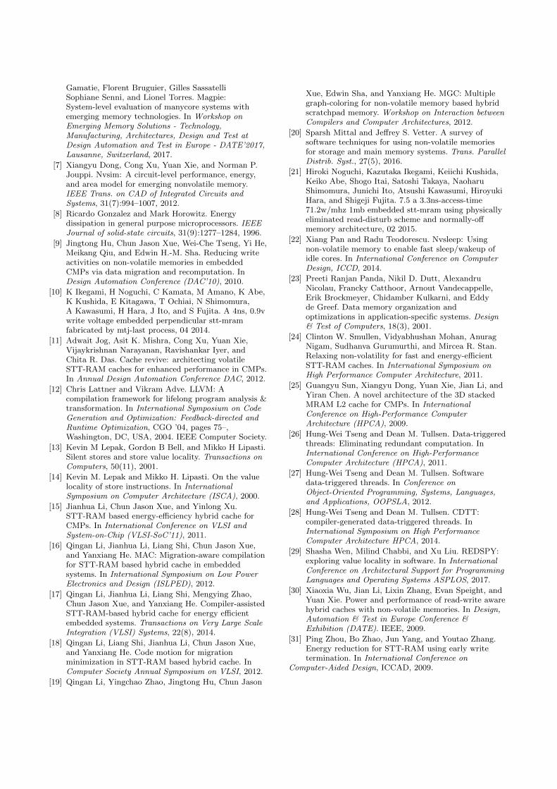
Gamatie, Florent Bruguier, Gilles SassatelliSophiane Senni, and Lionel Torres. Magpie:System-level evaluation of manycore systems withemerging memory technologies. In Workshop onEmerging Memory Solutions - Technology,Manufacturing, Architectures, Design and Test atDesign Automation and Test in Europe - DATE’2017,Lausanne, Switzerland, 2017.

[7] Xiangyu Dong, Cong Xu, Yuan Xie, and Norman P.Jouppi. Nvsim: A circuit-level performance, energy,and area model for emerging nonvolatile memory.IEEE Trans. on CAD of Integrated Circuits andSystems, 31(7):994–1007, 2012.

[8] Ricardo Gonzalez and Mark Horowitz. Energydissipation in general purpose microprocessors. IEEEJournal of solid-state circuits, 31(9):1277–1284, 1996.

[9] Jingtong Hu, Chun Jason Xue, Wei-Che Tseng, Yi He,Meikang Qiu, and Edwin H.-M. Sha. Reducing writeactivities on non-volatile memories in embeddedCMPs via data migration and recomputation. InDesign Automation Conference (DAC’10), 2010.

[10] K Ikegami, H Noguchi, C Kamata, M Amano, K Abe,K Kushida, E Kitagawa, T Ochiai, N Shimomura,A Kawasumi, H Hara, J Ito, and S Fujita. A 4ns, 0.9vwrite voltage embedded perpendicular stt-mramfabricated by mtj-last process, 04 2014.

[11] Adwait Jog, Asit K. Mishra, Cong Xu, Yuan Xie,Vijaykrishnan Narayanan, Ravishankar Iyer, andChita R. Das. Cache revive: architecting volatileSTT-RAM caches for enhanced performance in CMPs.In Annual Design Automation Conference DAC, 2012.

[12] Chris Lattner and Vikram Adve. LLVM: Acompilation framework for lifelong program analysis &transformation. In International Symposium on CodeGeneration and Optimization: Feedback-directed andRuntime Optimization, CGO ’04, pages 75–,Washington, DC, USA, 2004. IEEE Computer Society.

[13] Kevin M Lepak, Gordon B Bell, and Mikko H Lipasti.Silent stores and store value locality. Transactions onComputers, 50(11), 2001.

[14] Kevin M. Lepak and Mikko H. Lipasti. On the valuelocality of store instructions. In InternationalSymposium on Computer Architecture (ISCA), 2000.

[15] Jianhua Li, Chun Jason Xue, and Yinlong Xu.STT-RAM based energy-efficiency hybrid cache forCMPs. In International Conference on VLSI andSystem-on-Chip (VLSI-SoC’11), 2011.

[16] Qingan Li, Jianhua Li, Liang Shi, Chun Jason Xue,and Yanxiang He. MAC: Migration-aware compilationfor STT-RAM based hybrid cache in embeddedsystems. In International Symposium on Low PowerElectronics and Design (ISLPED), 2012.

[17] Qingan Li, Jianhua Li, Liang Shi, Mengying Zhao,Chun Jason Xue, and Yanxiang He. Compiler-assistedSTT-RAM-based hybrid cache for energy efficientembedded systems. Transactions on Very Large ScaleIntegration (VLSI) Systems, 22(8), 2014.

[18] Qingan Li, Liang Shi, Jianhua Li, Chun Jason Xue,and Yanxiang He. Code motion for migrationminimization in STT-RAM based hybrid cache. InComputer Society Annual Symposium on VLSI, 2012.

[19] Qingan Li, Yingchao Zhao, Jingtong Hu, Chun Jason

Xue, Edwin Sha, and Yanxiang He. MGC: Multiplegraph-coloring for non-volatile memory based hybridscratchpad memory. Workshop on Interaction betweenCompilers and Computer Architectures, 2012.

[20] Sparsh Mittal and Jeffrey S. Vetter. A survey ofsoftware techniques for using non-volatile memoriesfor storage and main memory systems. Trans. ParallelDistrib. Syst., 27(5), 2016.

[21] Hiroki Noguchi, Kazutaka Ikegami, Keiichi Kushida,Keiko Abe, Shogo Itai, Satoshi Takaya, NaoharuShimomura, Junichi Ito, Atsushi Kawasumi, HiroyukiHara, and Shigeji Fujita. 7.5 a 3.3ns-access-time71.2w/mhz 1mb embedded stt-mram using physicallyeliminated read-disturb scheme and normally-offmemory architecture, 02 2015.

[22] Xiang Pan and Radu Teodorescu. Nvsleep: Usingnon-volatile memory to enable fast sleep/wakeup ofidle cores. In International Conference on ComputerDesign, ICCD, 2014.

[23] Preeti Ranjan Panda, Nikil D. Dutt, AlexandruNicolau, Francky Catthoor, Arnout Vandecappelle,Erik Brockmeyer, Chidamber Kulkarni, and Eddyde Greef. Data memory organization andoptimizations in application-specific systems. Design& Test of Computers, 18(3), 2001.

[24] Clinton W. Smullen, Vidyabhushan Mohan, AnuragNigam, Sudhanva Gurumurthi, and Mircea R. Stan.Relaxing non-volatility for fast and energy-efficientSTT-RAM caches. In International Symposium onHigh Performance Computer Architecture, 2011.

[25] Guangyu Sun, Xiangyu Dong, Yuan Xie, Jian Li, andYiran Chen. A novel architecture of the 3D stackedMRAM L2 cache for CMPs. In InternationalConference on High-Performance ComputerArchitecture (HPCA), 2009.

[26] Hung-Wei Tseng and Dean M. Tullsen. Data-triggeredthreads: Eliminating redundant computation. InInternational Conference on High-PerformanceComputer Architecture (HPCA), 2011.

[27] Hung-Wei Tseng and Dean M. Tullsen. Softwaredata-triggered threads. In Conference onObject-Oriented Programming, Systems, Languages,and Applications, OOPSLA, 2012.

[28] Hung-Wei Tseng and Dean M. Tullsen. CDTT:compiler-generated data-triggered threads. InInternational Symposium on High PerformanceComputer Architecture HPCA, 2014.

[29] Shasha Wen, Milind Chabbi, and Xu Liu. REDSPY:exploring value locality in software. In InternationalConference on Architectural Support for ProgrammingLanguages and Operating Systems ASPLOS, 2017.

[30] Xiaoxia Wu, Jian Li, Lixin Zhang, Evan Speight, andYuan Xie. Power and performance of read-write awarehybrid caches with non-volatile memories. In Design,Automation & Test in Europe Conference &Exhibition (DATE). IEEE, 2009.

[31] Ping Zhou, Bo Zhao, Jun Yang, and Youtao Zhang.Energy reduction for STT-RAM using early writetermination. In International Conference on

Computer-Aided Design, ICCAD, 2009.

L

HEPSYCODE-RT : a Real-TimeExtension for an ESL HW/SWCo-Design Methodology

LI

HEPSYCODE-RT: a Real-Time Extension for an

ESL HW/SW Co-Design Methodology

Vittoriano Muttillo Center of Excellence DEWS

Via Vetoio, 1 L’Aquila, Italy

vittoriano.muttillo@graduate.univaq.it

Giacomo Valente Center of Excellence DEWS

Via Vetoio, 1 L’Aquila, Italy

giacomo.valente@graduate.univaq.it

Daniele Ciambrone Center of Excellence DEWS

Via Vetoio, 1 L’Aquila, Italy

daniele.ciambrone@student.univaq.it

Vincenzo Stoico Center of Excellence DEWS

Via Vetoio, 1 L’Aquila, Italy

vincenzo.stoico@student.univaq.it

Luigi Pomante Center of Excellence DEWS

Via Vetoio, 1 L’Aquila, Italy

luigi.pomante@univaq.it

ABSTRACT

This work 1 focuses on the definition of a methodology for

handling embedded real-time applications, starting from an

existing HW/SW co-design methodology able to support the

design of dedicated heterogeneous parallel systems. The state-of-

the-art related to similar tools and methodologies is presented and

the reference framework with the proposed extension to the real-

time world is introduced. A case study is then described to show a

design space exploration able to consider such an extension.

CCS CONCEPTS

• Hardware → Software tools for EDA; • Hardware →

Modeling and parameter extraction; Timing Simulation; DSE;

KEYWORDS

HW/SW Co-Design, Heterogeneous Parallel Systems, DSE, real-

time systems

1 INTRODUCTION

During the last years, the spread and importance of embedded

systems are increasing but it is still not yet possible to completely

engineer their system-level design flow. Designers commonly

adopt one or more system-level models (e.g. block diagrams,

UML, SystemC, etc.) to have a complete problem view, to

perform a check on HW/SW resources allocation and to validate

Permission to make digital or hard copies of all or part of this work for personal or

classroom use is granted without fee provided that copies are not made or distributed

for profit or commercial advantage and that copies bear this notice and the full

citation on the first page. Copyrights for components of this work owned by others

than ACM must be honored. Abstracting with credit is permitted. To copy otherwise,

or republish, to post on servers or to redistribute to lists, requires prior specific

permission and/or a fee. Request permissions from Permissions@acm.org.

RAPIDO, January 22-24, 2018, Manchester, United Kingdom

© 2018 Association for Computing Machinery.

ACM ISBN 978-1-4503-6417-1/18/01…$15.00

https://doi.org/10.1145/3180665.3180670

the design by simulating the system behavior. In this scenario, SW

tools to support designers to reduce costs and overall complexity

of systems development are even more of fundamental

importance. Unfortunately, there are no fully engineered general

methodologies defined for this purpose and often the best option

is still to refer to experienced designer indications to take

advantage of empirical criteria and qualitative assessments. For

example, systems based on heterogeneous multi-processor

architectures (Heterogeneous Multi-Processor Systems, HMPS)

have been recently exploited for a wide range of application

domains, especially in the System-on-Chip (SoC) form factor (e.g.

[2]). In particular, such architectures are often used to implement

Dedicated Systems (DS), i.e. digital electronic systems with an

application-specific HW/SW architecture designed to satisfy a

priori known application with F/NF requirements. In such a case,

they are called Dedicated Heterogeneous Multi-Processor

Systems (D-HMPS). D-HMPS are so complex that the adopted

HW/SW Co-Design Methodology plays a major role in

determining the success of a product. The situation is even worse

if the considered system is a hard/soft real-time one. In such a

case, time constraints are normally defined considering the worst

possible case (hard) or an average situation (soft).

In such a context, this work focuses on the definition of a

HW/SW co-design methodology and the development of a related

prototypal tool to improve the design time of embedded real-time

applications. Specifically, the whole framework drives the

designer from an Electronic System-Level (ESL) behavioral

model, with related NF requirements, including real-time ones, to

the final HW/SW implementation, considering specific HW

technologies, scheduling policies and Inter-Process

Communication (IPC) mechanisms. The remainder of the paper is

organized as follows: Section II provides an overview of HW/SW

co-design tools related to embedded real-time computing systems.

Section III describes the reference HW/SW Co-Design

methodology, whereas Section IV discusses the extension to adapt

it to the real-time world. Section V presents a case study that

shows a design space exploration able to consider such an

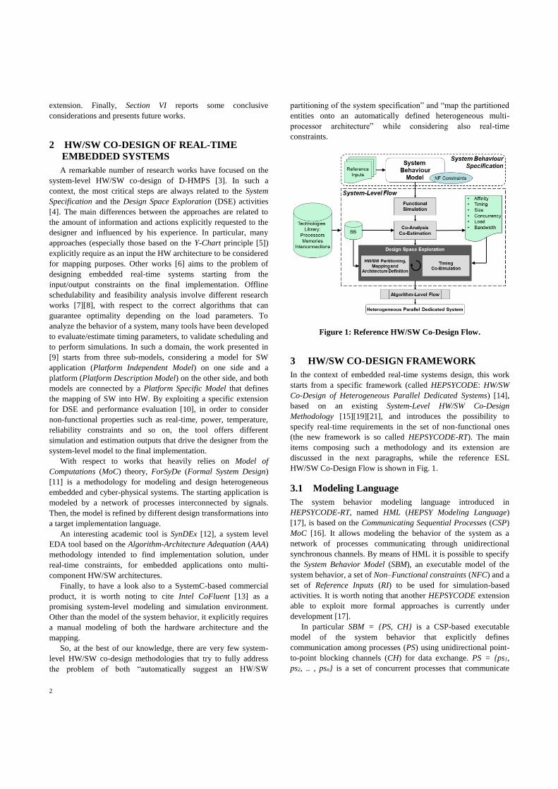
2

extension. Finally, Section VI reports some conclusive

considerations and presents future works.

2 HW/SW CO-DESIGN OF REAL-TIME

EMBEDDED SYSTEMS

A remarkable number of research works have focused on the

system-level HW/SW co-design of D-HMPS [3]. In such a

context, the most critical steps are always related to the System

Specification and the Design Space Exploration (DSE) activities

[4]. The main differences between the approaches are related to

the amount of information and actions explicitly requested to the

designer and influenced by his experience. In particular, many

approaches (especially those based on the Y-Chart principle [5])

explicitly require as an input the HW architecture to be considered

for mapping purposes. Other works [6] aims to the problem of

designing embedded real-time systems starting from the

input/output constraints on the final implementation. Offline

schedulability and feasibility analysis involve different research

works [7][8], with respect to the correct algorithms that can

guarantee optimality depending on the load parameters. To

analyze the behavior of a system, many tools have been developed

to evaluate/estimate timing parameters, to validate scheduling and

to perform simulations. In such a domain, the work presented in

[9] starts from three sub-models, considering a model for SW

application (Platform Independent Model) on one side and a

platform (Platform Description Model) on the other side, and both

models are connected by a Platform Specific Model that defines

the mapping of SW into HW. By exploiting a specific extension

for DSE and performance evaluation [10], in order to consider

non-functional properties such as real-time, power, temperature,

reliability constraints and so on, the tool offers different

simulation and estimation outputs that drive the designer from the

system-level model to the final implementation.

With respect to works that heavily relies on Model of

Computations (MoC) theory, ForSyDe (Formal System Design)

[11] is a methodology for modeling and design heterogeneous

embedded and cyber-physical systems. The starting application is

modeled by a network of processes interconnected by signals.

Then, the model is refined by different design transformations into

a target implementation language.

An interesting academic tool is SynDEx [12], a system level

EDA tool based on the Algorithm-Architecture Adequation (AAA)

methodology intended to find implementation solution, under

real-time constraints, for embedded applications onto multi-

component HW/SW architectures.

Finally, to have a look also to a SystemC-based commercial

product, it is worth noting to cite Intel CoFluent [13] as a

promising system-level modeling and simulation environment.

Other than the model of the system behavior, it explicitly requires

a manual modeling of both the hardware architecture and the

mapping.

So, at the best of our knowledge, there are very few system-

level HW/SW co-design methodologies that try to fully address

the problem of both “automatically suggest an HW/SW

partitioning of the system specification” and “map the partitioned

entities onto an automatically defined heterogeneous multi-

processor architecture” while considering also real-time

constraints.

Figure 1: Reference HW/SW Co-Design Flow.

3 HW/SW CO-DESIGN FRAMEWORK

In the context of embedded real-time systems design, this work

starts from a specific framework (called HEPSYCODE: HW/SW

Co-Design of Heterogeneous Parallel Dedicated Systems) [14],

based on an existing System-Level HW/SW Co-Design

Methodology [15][19][21], and introduces the possibility to

specify real-time requirements in the set of non-functional ones

(the new framework is so called HEPSYCODE-RT). The main

items composing such a methodology and its extension are

discussed in the next paragraphs, while the reference ESL

HW/SW Co-Design Flow is shown in Fig. 1.

3.1 Modeling Language

The system behavior modeling language introduced in

HEPSYCODE-RT, named HML (HEPSY Modeling Language)

[17], is based on the Communicating Sequential Processes (CSP)

MoC [16]. It allows modeling the behavior of the system as a

network of processes communicating through unidirectional

synchronous channels. By means of HML it is possible to specify

the System Behavior Model (SBM), an executable model of the

system behavior, a set of Non–Functional constraints (NFC) and a

set of Reference Inputs (RI) to be used for simulation-based

activities. It is worth noting that another HEPSYCODE extension

able to exploit more formal approaches is currently under

development [17].

In particular SBM = {PS, CH} is a CSP-based executable

model of the system behavior that explicitly defines

communication among processes (PS) using unidirectional point-

to-point blocking channels (CH) for data exchange. PS = {ps1,

ps2, .. , psn} is a set of concurrent processes that communicate

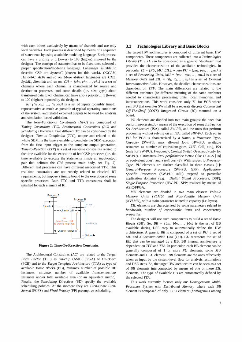
3

with each others exclusively by means of channels and use only

local variables. Each process is described by means of a sequence

of statements by using a suitable modeling language. Each process

can have a priority p: 1 (lower) to 100 (higher) imposed by the

designer. The concept of statement has to be fixed once selected a

proper specification/modeling language. Languages suitable to

describe CSP are SystemC (chosen for this work), OCCAM,

Handel-C, ADA and so on. More abstract languages are UML,

SysML, Simulink and so on. CH = {ch1, ch2, .. , chn} is a set of

channels where each channel is characterized by source and

destination processes, and some details (i.e. size, type) about

transferred data. Each channel can have also a priority p: 1 (lower)

to 100 (higher) imposed by the designer.

RI: {(i1 ,o1), …, (in ,on)} is a set of inputs (possibly timed),

representative as much as possible of typical operating conditions

of the system, and related expected outputs to be used for analysis

and simulation-based validation.

The Non–Functional Constraints (NFC) are composed of

Timing Constraints (TC), Architectural Constraints (AC) and

Scheduling Directives. Two different TC can be considered by the

designer: Time-to-Completion (TTC), unique and related to the

whole SBM, is the time available to complete the SBM execution

from the first input trigger to the complete output generation;

Time-to-Reaction (TTR) is a set of real-time constraints related to

the time available for the execution of leaf CSP processes (i.e. the

time available to execute the statements inside an input/output

pair that delimits the CPS process main body, see Fig. 2).

Different leaf processes can have different associated TTR. This

real-time constraints are not strictly related to classical RT

requirements, but impose a timing bound to the execution of some

specific processes. Both TTC and TTR constraints shall be

satisfied by each element of RI.

Figure 2: Time-To-Reaction Constrain.

The Architectural Constraints (AC) are related to the Target

Form Factor (TFF) as On-chip (ASIC, FPGA) or On-Board

(PCB) and to the Target Template Architecture (TTA) as type of

available Basic Blocks (BB), min/max number of possible BB

instances, min/max number of available Interconnections

instances and/or total available area (or an equivalent metric).

Finally, the Scheduling Directives (SD) specify the available

scheduling policies. At the moment they are First-Come First-

Served (FCFS) and Fixed Priority (FP) preemptive scheduling.

3.2 Technologies Library and Basic Blocks

The target HW architectures is composed of different basic HW

components. These components are collected into a Technologies

Library (TL). TL can be considered as a generic “database” that

provides the characterization of the available technologies. In

particular TL = {PU, MU, EIL}, where PU = {pu1, pu2, .. , pup} is

a set of Processing Units, MU = {mu1, mu2, .. , mum} is a set of

Memory Units and EIL = {il1, il2, .. , ilc} is a set of External

Interconnection Links. However, the detailed characterizations are

dependent on TFF. The main differences are related to the

different attributes (or different meaning of the same attribute)

needed to characterize processing units, local memories, and

interconnections. This work considers only TL for PCB where

each PU that executes SW shall be a separate discrete Commercial

Off-The-Shelf (COTS) Integrated Circuit (IC) mounted on a

board.

PU elements are divided into two main groups: the ones that

perform processing by means of the execution of some Instruction

Set Architecture (ISA), called SW-PU, and the ones that perform

processing without relying on an ISA, called HW-PU. Each pui in

PU for PCB is characterized by a Name, a Processor Type,

Capacity (SW-PU: max allowed load; HW-PU: available

resources as number of equivalent-gates, LUT, Cell, etc.), ISA

(only for SW-PU), Frequency, Context Switch Overhead (only for

SW-PU), a statement-level performance metric (like CC4CS [18]

or equivalent ones), and a unit cost (€). With respect to Processor

Type, PU elements are further classified in three classes [1]:

General-Purpose Processors (SW-PU: GPP); Application-

Specific Processors (SW-PU: ASP) targeted to particular

application domains (e.g. Digital Signal Processors, DSP);

Single-Purpose Processor (HW-PU: SPP; realized by means of

ASIC/FPGA.

MU elements are divided in two main classes: Volatile

Memory Units (VLMU) and Non-Volatile Memory Units

(NVLMU), with a main parameter related to capacity (i.e. bytes).

EIL elements are characterized by some parameters related to

bandwidth, number of connectable items and concurrency

properties.

The designer will use such components to build a set of Basic

Blocks (BB). So, BB = {bb1, bb2, .. , bbb} is the set of BB

available during DSE step to automatically define the HW

architecture. A generic BB is composed of a set of PU, a set of

MU and a Communication Unit (CU). CU represents the set of

EIL that can be managed by a BB. BB internal architecture is

dependent on TFF and TTA. In particular, each BB element can be

generally composed of 1 or more PU elements, some MU

elements and 1 CU element. BB elements are the ones effectively

taken as input by the system-level flow for analysis, estimations

and DSE steps. So, the target HW architecture can be seen as a set

of BB elements interconnected by means of one or more EIL

elements. The type of available BB are automatically defined by

the selected TTA.

This work currently focuses only on: Homogeneous Multi-

Processor System with Distributed Memory where each BB

element is composed of only 1 PU element (homogenous among

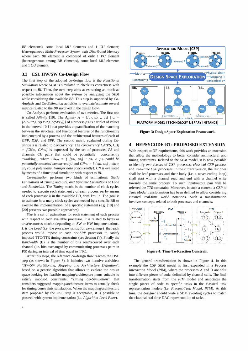
4

BB elements), some local MU elements and 1 CU element;

Heterogeneous Multi-Processor System with Distributed Memory

where each BB element is composed of only 1 PU element

(heterogeneous among BB elements), some local MU elements

and 1 CU element.

3.3 ESL HW/SW Co-Design Flow

The first step of the adopted co-design flow is the Functional

Simulation where SBM is simulated to check its correctness with

respect to RI. Then, the next step aims at extracting as much as

possible information about the system by analyzing the SBM

while considering the available BB. This step is supported by Co-

Analysis and Co-Estimation activities to evaluate/estimate several

metrics related to the BB involved in the design flow.

Co-Analysis performs evaluation of two metrics. The first one

is called Affinity [19]. The Affinity A = {[a1, a2, .. an] | ai =

[A(GPPi), A(DSPi), A(SPPi)]} of a process psi is a triplet of values

in the interval [0,1] that provides a quantification of the matching

between the structural and functional features of the functionality

implemented by a process and the architectural features of each of

GPP, DSP, and SPP. The second metric evaluated during Co-

analysis is related to Concurrency. The concurrency CN(PS, CH)

= [CNPS, CNCH] is expressed by the set of processes PS and

channels CH pairs that could be potentially concurrently

“working”, where CNPS = { [psi, psj] : psi ˄ psj could be

potentially executed concurrently} and CNCH = { [chi, chj] : chi ˄

chj could potentially transfer data concurrently}. CN is evaluated

by means of a functional simulation with respect to RI.

Co-estimation performs two kinds of estimations: Static

Estimations of Timing and Size, and Dynamic Estimations of Load

and Bandwidth. The Timing metric is the number of clock cycles

needed to execute each statement j of each process psi by means

of each processor k in the available BB, with k=1..n. The goal is

to estimate how many clock cycles are needed by a specific BB to

execute the implementation of a specific statement (e.g. [18] and

[20] presents two possible approaches).

Size is a set of estimations for each statement of each process

with respect to each available processor. It is related to bytes or

area/resources metrics depending on SW or HW implementations.

L is the Load (i.e. the processor utilization percentage) that each

process would impose to each not-SPP processor to satisfy

imposed TTC/TTR timing constraints (see Section IV). Finally the

Bandwidth (B) is the number of bits sent/received over each

channel (i.e. bits exchanged by communicating processes pairs in

PS) during an interval of time equal to TTC.

After this steps, the reference co-design flow reaches the DSE

step (as shown in Figure 3). It includes two iterative activities:

“HW/SW Partitioning, Mapping and Architecture Definition”,

based on a genetic algorithm that allows to explore the design

space looking for feasible mapping/architecture items suitable to

satisfy imposed constraints; “Timing Co-Simulation”, that

considers suggested mapping/architecture items to actually check

for timing constraints satisfaction. When the mapping/architecture

item proposed by the DSE step is acceptable, it is possible to

proceed with system implementation (i.e. Algorithm-Level Flow).

Figure 3: Design Space Exploration Framework.

4 HEPSYCODE-RT: PROPOSED EXTENSION

With respect to NF requirements, this work provides an extension

that allow the methodology to better consider architectural and

timing constraints. Related to the SBM model, it is now possible

to identify two classes of CSP processes: classical CSP process

and real-time CSP processes. In the current version, the last ones

shall be leaf processes and their body (i.e. a never-ending loop)

shall start with a channel read and end with a channel write

towards the same process. To such input/output pair will be

referred the TTR constraint. Moreover, in such a context, a CSP to

Task Model transformation has been defined to allow considering

classical real-time world notations. Such a transformation

involves concepts related to both processes and channels.

Figure 4: Time-To-Reaction Constrain.

The general transformation is shown in Figure 4. In this

example the CSP SBM model is first expanded in a Process

Interaction Model (PIM), where the processes A and B are split

into different pieces of code, delimited by channel calls. The final

transformation starts from the PIM model and associates the

single pieces of code to specific tasks in the classical task

representation models (i.e. Process-Task Model, PTM). At this

time, the designer should write a SBM avoiding cycles to match

the classical real-time DAG representation of tasks.

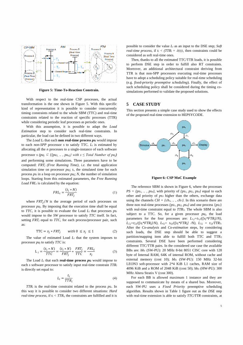
5

Figure 5: Time-To-Reaction Constrain.

With respect to the real-time CSP processes, the actual

transformation is the one shown in Figure 5. With this specific

kind of representation it is possible to consider concurrently

timing constraints related to the whole SBM (TTC) and real-time

constraints related to the reaction of specific processes (TTR)

while considering periodic leaf processes as periodic ones.

With this assumption, it is possible to adapt the Load

Estimation step to consider such real-time constraints. In

particular, the load can be defined in two different ways.

The Load Li that each non real-time process psi would impose

to each non-SPP processor s to satisfy TTC. Li is estimated by

allocating all the n processes to a single-instance of each software

processor s (puj ⊆ {[pu1, .. , pus]} with s ≤ Total Number of puj)

and performing some simulations. Three parameters have to be

computed: FRTj (Free Running Time), i.e. the total application

simulation time on processor puj; ti, the simulated time for each

process psi in a loop on processor puj; N, the number of simulation

loops. Starting from this estimated parameters, the Free Running

Load FRLi is calculated by the equation:

𝐹𝑅𝐿𝑖 =(𝑡𝑖 ∗ 𝑁)

𝐹𝑅𝑇𝑗 (1)

where 𝐹𝑅𝑇𝑗 𝑁⁄ is the average period of each processes on

processor puj. By imposing that the execution time shall be equal

to TTC, it is possible to evaluate the Load Li that processes psi

would impose to the SW processor to satisfy TTC itself. In fact,

setting FRTj equal to TTC, for each process/processor pair, such

as:

TTC = 𝑥𝑗 ∗ 𝐹𝑅𝑇𝑗 𝑤𝑖𝑡ℎ 0 ≤ 𝑥𝑗 ≤ 1 (2)

The value of estimated Load Li that the system imposes to

processor puj to satisfy TTC is:

L 𝑖 =(𝑡𝑖 ∗ 𝑁)

𝑇𝑇𝐶=

(𝑡𝑖 ∗ 𝑁)

𝐹𝑅𝑇𝑗∗

𝐹𝑅𝑇𝑗

𝑇𝑇𝐶=

𝐹𝑅𝐿𝑗

𝑥𝑗 (3)

The Load Li that each real-time process psi would impose to

each s software processor to satisfy input real-time constrain TTRi

is directly set equal to:

𝐿𝑖 =𝑡𝑖

𝑇𝑇𝑅𝑖 (4)

TTRi is the real-time constraint related to the process psi. In

this way it is possible to consider two different situations: Hard

real-time process, if ti < TTRi, the constraints are fulfilled and it is

possible to consider the value Li as an input to the DSE step; Soft

real-time process, if ti < (TTRi + δ(t)), then constraints could be

considered as soft real-time ones.

Then, thanks to all the estimated TTC/TTR loads, it is possible

to perform DSE step in order to fulfill also RT constraints.

Moreover, an additional architectural constraint deriving from

TTR is that non-SPP processors executing real-time processes

have to adopt a scheduling policy suitable for real-time scheduling

(e.g. fixed-priority preemptive scheduling). Finally, the effect of

such scheduling policy shall be considered during the timing co-

simulations performed to validate the proposed solutions.

5 CASE STUDY

This section presents a simple case study used to show the effects

of the proposed real-time extension to HEPSYCODE.

Figure 6: CSP MoC Example

The reference SBM is shown in Figure 6, where the processes

PS = {ps1, .. , ps4}, with priority of {ps1, ps2, ps4} equal to each

other and priority of ps3 higher than the others, exchange data

using the channels CH = {ch1, .. , ch7}. In this scenario there are

three non real-time processes {ps1, ps2, ps4} and one process {ps3}

with real-time constraint equal to TTR3. The whole SBM is also

subject to a TTC. So, for a given processor puj, the load

parameters for the four processes are: L1,j=t1,j/([xj*FTRj]/N),

L2,j=t2,j/([xj*FTRj]/N), L4,j= t4,j/([xj*FTRj] /N), L3,j = t3,j/TTR3.

After the Co-analysis and Co-estimation steps, by considering

such loads, the DSE step should be able to suggest a

partition/mapping item able to fulfill both TTC and TTR3

constraints. Several DSE have been performed considering

different TTC/TTR pairs. In the considered use case the available

BBs are: bb1 (SW-PU): 20 MHz 8-bit 8051 CISC core with 128

byte of Internal RAM, 64K of internal ROM, without cache and

external memory (cost 10); bb2 (SW-PU): 150 MHz 32-bit

LEON3 soft-processor with 2*4 KiB L1 caches, RAM size of

4096 KiB and a ROM of 2048 KiB (cost 50); bb3 (HW-PU): 300

MHz Altera Stratix V (cost 300).

For each BB is allowed maximum 1 instance and they are

supposed to communicate by means of a shared bus. Moreover,

each SW-PU uses a Fixed Priority preemptive scheduling

algorithm. Results shown in Table 1 figure out as the DSE step

with real-time extension is able to satisfy TTC/TTR constraints, at

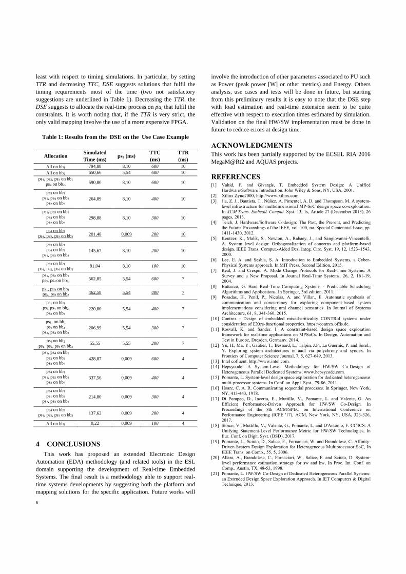
6

least with respect to timing simulations. In particular, by setting

TTR and decreasing TTC, DSE suggests solutions that fulfil the

timing requirements most of the time (two not satisfactory

suggestions are underlined in Table 1). Decreasing the TTR, the

DSE suggests to allocate the real-time process on puj that fulfil the

constraints. It is worth noting that, if the TTR is very strict, the

only valid mapping involve the use of a more expensive FPGA.

Table 1: Results from the DSE on the Use Case Example

Allocation Simulated

Time (ms) ps3 (ms)

TTC

(ms)

TTR

(ms)

All on bb1 794,88 8,10 600 10

All on bb2 650,66 5,54 600 10

ps1, ps2, ps3 on bb1

ps4 on bb2, 590,80 8,10 600 10

ps3 on bb1

ps1, ps4 on bb2

ps2 on bb3 264,89 8,10 400 10

ps1, ps3 on bb1

ps4 on bb2

ps2 on bb3 298,88 8,10 300 10

ps4 on bb1

ps1, ps2, ps3 on bb3 201,48 0,009 200 10

ps3 on bb1

ps4 on bb2

ps1, ps2 on bb3 145,67 8,10 200 10

ps3 on bb1

ps1, ps2, ps4 on bb3 81,04 8,10 100 10

ps1, ps2 on bb1

ps3, ps4 on bb2, 562,85 5,54 600 7

ps1, pu4 on bb1

ps2, ps3 on bb2 462,58 5,54 400 7

ps1 on bb1

ps3, ps4 on bb2

ps2 on bb3 220,80 5,54 400 7

ps1, on bb1

ps3 on bb2

ps2, ps4 on bb3

206,99 5,54 300 7

ps3 on bb2

ps1, ps2, ps4 on bb3 55,55 5,55 200 7

ps1, ps4 on bb1

ps2 on bb2

ps3 on bb3

428,87 0,009 600 4

ps4 on bb1

ps1, ps2 on bb2

ps3 on bb3 337,56 0,009 400 4

ps4 on bb1

ps1 on bb2

ps2, ps3 on bb3 214,80 0,009 300 4

ps4 on bb2

ps1, ps2, ps3 on bb3 137,62 0,009 200 4

All on bb3 0,22 0,009 100 4

4 CONCLUSIONS

This work has proposed an extended Electronic Design

Automation (EDA) methodology (and related tools) in the ESL

domain supporting the development of Real-time Embedded

Systems. The final result is a methodology able to support real-

time systems developments by suggesting both the platform and

mapping solutions for the specific application. Future works will

involve the introduction of other parameters associated to PU such

as Power (peak power [W] or other metrics) and Energy. Others

analysis, use cases and tests will be done in future, but starting

from this preliminary results it is easy to note that the DSE step

with load estimation and real-time extension seem to be quite

effective with respect to execution times estimated by simulation.

Validation on the final HW/SW implementation must be done in

future to reduce errors at design time.

ACKNOWLEDGMENTS

This work has been partially supported by the ECSEL RIA 2016

MegaM@Rt2 and AQUAS projects.

REFERENCES [1] Vahid, F. and Givargis, T. Embedded System Design: A Unified

Hardware/Software Introduction. John Wiley & Sons, NY, USA, 2001.

[2] Xilinx Zynq7000, http://www.xilinx.com.

[3] Jia, Z. J., Bautista, T., Núñez, A. Pimentel, A. D. and Thompson, M. A system-

level infrastructure for multidimensional MP-SoC design space co-exploration.

In ACM Trans. Embedd. Comput. Syst. 13, 1s, Article 27 (December 2013), 26

pages, 2013.

[4] Teich, J. Hardware/Software Codesign: The Past, the Present, and Predicting

the Future. Proceedings of the IEEE, vol. 100, no. Special Centennial Issue, pp.

1411-1430, 2012.

[5] Keutzer, K., Malik, S., Newton, A., Rabaey, J., and Sangiovanni-Vincentelli,

A. System level design: Orthogonalization of concerns and platform-based

design. IEEE Trans. Comput.-Aided Des. Integ. Circ. Syst. 19, 12, 1523–1543,

2000.

[6] Lee, E. A. and Seshia, S. A. Introduction to Embedded Systems, a Cyber-

Physical Systems approach. In MIT Press, Second Edition, 2015.

[7] Real, J. and Crespo, A. Mode Change Protocols for Real-Time Systems: A

Survey and a New Proposal. In Journal Real-Time Systems, 26, 2, 161-19,

2004.

[8] Buttazzo, G. Hard Real-Time Computing Systems - Predictable Scheduling

Algorithms and Applications. In Springer, 3rd edition, 2011.

[9] Posadas, H., Penil, P., Nicolas, A. and Villar., E. Automatic synthesis of

communication and concurrency for exploring component-based system

implementations considering uml channel semantics. In Journal of Systems

Architecture, 61, 8, 341-360, 2015.

[10] Contrex - Design of embedded mixed-criticality CONTRol systems under

consideration of EXtra-functional properties. https://contrex.offis.de.

[11] Rosvall, K. and Sander. I. A constraint-based design space exploration

framework for real-time applications on MPSoCs. In Design, Automation and

Test in Europe, Dresden, Germany. 2014.

[12] Yu, H., Ma, Y., Gautier, T., Besnard, L., Talpin, J.P., Le Guernic, P. and Sorel.,

Y. Exploring system architectures in aadl via polychrony and syndex. In

Frontiers of Computer Science Journal, 7, 5, 627-649, 2013.

[13] Intel cofluent. http://www.intel.com.

[14] Hepsycode: A System-Level Methodology for HW/SW Co-Design of

Heterogeneous Parallel Dedicated Systems, www.hepsycode.com.

[15] Pomante, L. System-level design space exploration for dedicated heterogeneous

multi-processor systems. In Conf. on Appl. Syst., 79-86, 2011.

[16] Hoare, C. A. R. Communicating sequential processes. In Springer, New York,

NY, 413-443, 1978.

[17] Di Pompeo, D., Incerto, E., Muttillo, V., Pomante, L. and Valente, G. An

Efficient Performance-Driven Approach for HW/SW Co-Design. In

Proceedings of the 8th ACM/SPEC on International Conference on

Performance Engineering (ICPE '17), ACM, New York, NY, USA, 323-326,

2017.

[18] Stoico, V., Muttillo, V., Valente, G., Pomante, L. and D'Antonio, F. CC4CS: A

Unifying Statement-Level Performance Metric for HW/SW Technologies, In

Eur. Conf. on Digit. Syst. (DSD), 2017.

[19] Pomante, L., Sciuto, D., Salice, F., Fornaciari, W. and Brandolese, C. Affinity-

Driven System Design Exploration for Heterogeneous Multiprocessor SoC, In

IEEE Trans. on Comp., 55, 5, 2006.

[20] Allara, A., Brandolese, C., Fornaciari, W., Salice, F. and Sciuto, D. System-

level performance estimation strategy for sw and hw, In Proc. Int. Conf. on

Comp., Austin, TX, 48-53, 1998.

[21] Pomante, L. HW/SW Co-Design of Dedicated Heterogeneous Parallel Systems:

an Extended Design Space Exploration Approach. In IET Computers & Digital

Technique, 2013.

LVIII

NVMain Extension for Multi-LevelCache Systems

LIX

NVMain Extension for Multi-Level Cache Systems

Asif Ali Khan, Fazal Hameed and Jeronimo CastrillonChair For Compiler Construction

Technische Universität Dresden, Germany{ asif_ali.khan, fazal.hameed, jeronimo.castrillon }@tu-dresden.de

ABSTRACTIn this paper, we present an extension of the NVMain mem-ory simulator. The objective is to facilitate computer ar-chitects to model complex memory designs for future com-puting systems in an accurate simulation framework. Thesimulator supports commodity memory models for DRAMas well as emerging non-volatile memories technologies suchSTT-RAM, ReRAM, PCRAM and hybrid models. The cur-rent publicly available version of NVMain, NVMain 2.0,offers support for main memory (using DRAM and NVMtechnologies) and a die-stacked DRAM cache. We extendthe cache model of the simulator by introducing an SRAMcache model and its supporting modules. With this addition,designers can model hybrid multi-level cache hierarchies byusing the die-stacked DRAM cache and SRAM caches. Weprovide a reference implementation of an optimized cache or-ganization scheme for die-stacked DRAM cache along witha tag-cache unit that, together, reduces cache miss latency.To enable integration of the new features in the existingmemory hierarchy, we make necessary changes to the mem-ory controller. We provide functional verification of the newmodules and put forward our approach for timing and powerverification. We run random mixes of the SPEC2006 bench-marks and observe±10% difference in simulation results.

CCS Concepts•Memory System Design → Memory System Hirarichy;Memory Technologies; •Memory Simulators→ SimulatorAccuracy; Design options; Simulator Speed; Extendibility;Resilience;

KeywordsMemory Simulator; SRAM Cache; Cache Organization; RowBuffer; Tag-cache

Permission to make digital or hard copies of all or part of this work for personal orclassroom use is granted without fee provided that copies are not made or distributedfor profit or commercial advantage and that copies bear this notice and the full cita-tion on the first page. Copyrights for components of this work owned by others thanthe author(s) must be honored. Abstracting with credit is permitted. To copy other-wise, or republish, to post on servers or to redistribute to lists, requires prior specificpermission and/or a fee. Request permissions from permissions@acm.org.

RAPIDO, January 22–24, 2018, Manchester, United Kingdomc© 2018 Copyright held by the owner/author(s). Publication rights licensed to ACM.

978-1-4503-6417-1/18/01. . . $15.00

DOI: https://doi.org/10.1145/3180665.3180672

1. INTRODUCTIONCPU and memory system are the two most important

components in any computing system. From the perfor-mance perspective, both components are strictly interlinked.CPU frequency has rapidly increased in the past decadewhile frequency of the memory system has not scaled upat the same pace. The memory system has always been onthe down side due its high access time and relatively lowoperating frequency, becoming a major bottleneck in mod-ern days computing systems. The rise of multi-core sys-tems has further worsened this problem and the availableper core capacity and per core bandwidth has diminishedfurther. Commodity memory technologies such as DRAMare unable to fill this ever-increasing processor memory gap.

DRAM is highly criticized for being expensive in termsof power as well. The major factor that dominates DRAMpower dissipation is its periodic refreshes, background andleakage power. The newly emerged non-volatile memory(NVM) technologies such as spin-torque-transfer random-access memory (STT-RAM), phase-change random-accessmemory (PCRAM), and resistive random-access memory(ReRAM) are believed to alleviate these limitations. Theyhave been advocated as potential DRAM replacements atvarious levels (main memory, die-stacked cache). Whilethese technologies could supplement or supersede conven-tional memory technologies at various levels in the memoryhierarchy, they have their own limitations. Simply replace-ment of DRAM with NVM technologies is not a viable op-tion because the latter suffers from high write energy andwrite endurance issues.

This opens up new research directions and calls for ex-ploration of appropriate memory technologies at each mem-ory level. An ideal memory system would use the best ofmany memory technologies and fulfill the diverse demandsof modern days applications. To design such system, it is vi-tal for computer architects to use simulation tools and studythe suitability of each technology. NVMain [24] is one suchsimulator that provides support for both DRAM and NVMtechnologies. It models energy and cycle accurate operationsof main memory system. In its extended version NVMain2.0 [25], die-stacked DRAM cache was introduced with theAlloy [26] model.

In this paper, we present extensions for the publicly avail-able version of NVMain (NVMain 2.0) simulator. We pro-vide a reference implementation of a new SRAM cache whichcould be used at various cache levels. For die-stacked cache,we provide implementation of various latency optimizations.To demonstrate this extension, we model a recently proposed

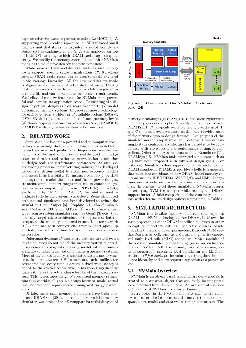
high associativity cache organization called LAMOST [9]. Asupporting module called tag-cache (an SRAM based smallmemory unit that stores the tag information of recently ac-cessed sets as explained in [14, 9, 20]) is employed on topof LAMOST to mitigate high DRAM cache tag lookup la-tency. We modify the memory controller and other NVMainmodules to make provision for the new extensions.

While some of these architectural features such as tag-cache support specific cache organizations [17, 9], otherssuch as SRAM cache model can be used to model any levelin the memory hierarchy. All the new modules are madeconfigurable and can be enabled or disabled easily. Config-uration parameters of each individual module are passed ina config file and can be varied as per design requirements.We believe these new features make NVMain more power-ful and increase its application scope. Considering the de-sign objectives, designers have more freedom to (a) modelcustomized memory systems (b) choose memory technologyfor each level from a wider list of available options (DRAM,NVM, SRAM) (c) select the number of cache/memory levels(d) choose appropriate cache organization (Alloy, LAMOST,LAMOST with tag-cache) for die-stacked memory.

2. RELATED WORKSimulation has become a powerful tool in computer archi-

tecture community that empowers designers to model theirdesired systems and predict the design objectives before-hand. Architectural simulation is mainly used for designspace exploration and performance evaluation consideringall design goals and performance parameters. As such, ev-ery leading processor manufacturing industry has developedits own simulation tool(s) to model new processor modelsand assess their feasibility. For instance, Mambo [4] by IBMis designed to model their past and future power designs.Its architectural support ranges from cell to embedded sys-tem to supercomputer (BlueGene, POWER7). Similarly,SimNow [2] by AMD and HAsim [23] by Intel are used toevaluate their future systems respectively. Some high speedarchitectural simulators have been developed to reduce thesimulation time. Sniper [5], Graphite [21], SlackSimslack-sim, P-Mambo [30] and COTSon [1] are to name a few.Open source system simulators such as Gem5 [3] exist thatnot only target micro-architecture of the processor but en-compasses the whole system architecture. In a recent work[19], Gem5 has been coupled with SystemC that opens upa whole new set of options for system level design spaceexploration.

Unfortunately, some of these micro-architecture and system-level simulators do not model the memory system in detail.They consider a simplistic memory model without consid-ering the complex organization of modern memory systems.More often, a fixed latency is associated with a memory ac-cess. In more advanced CPU simulators, bank conflicts areconsidered and every time it occurs, a fixed wait latency isadded to the overall access time. This model significantlyunderestimates the actual characteristic of the memory sys-tem. This necessitates design of specialized memory simula-tors that consider all possible design features, model actualbus latencies, and report correct timing and energy param-eters.

Of late, many such memory simulators have been pub-lished. DRAMSim [29], the first publicly available memorysimulator, was designed to offer support for multiple types of

Ranks

Command:RAS, CAS, PRE,

REF, PowerDown, PwerUp

OnchipOffchip(optical)

Address Mapping

Translator

prefetcher visualizer

Request Scheduling

Ref

resh

End

ura

nce

Simulator Interface

QueueRequest

GEM

5, T

race

File

FFindStarvedReqFindCloseBank

FindRBHitFindOldestReq

Sub Array

En

du

ran

ce

BankCache Bank

Bank

Interconnect

Memory Controller

Figure 1: Overview of the NVMain Architec-ture [24]

memory technologies (SDRAM, DDR) and allow explorationof memory system concepts. Presently, its extended versionDRAMSim2 [27] is openly available and is broadly used. Itis a C++ based cycle-accurate model that provides mostof the memory system design features. Design goals of thesimulator were to keep it small and portable. However, thissimplicity in controller architecture has barred it to be com-parable with more recent and performance optimized con-trollers. Other memory simulators such as Ramulator [16],DRAMSys [15], NVMain and integrated simulators such as[28] have been proposed with different design goals. Forinstance, Ramulator offers support for an extended list ofDRAM standards. DRAMSys provides a holistic frameworkthat takes into consideration new DRAM based memory so-lutions such as JDEC DDR4, WIDE I/O, and HMC. It cap-tures new aspects such as temperature and retention fail-ures. In contrast to all these simulators, NVMain focuseson emerging NVM technologies while keeping the DRAMsupport intact. A brief comparison of these memory simula-tors with reference to design options is presented in Table 1.

3. SIMULATOR ARCHITECTURENVMain is a flexible memory simulator that supports

DRAM and NVM technologies. For DRAM, it follows thesame approach as other DRAM specific simulators in orderto capture important features. For NVM devices, besidemodeling timing and power parameters, it models NVM spe-cific features as well; such as endurance, high write energy,and multi-level cells (MLC) capability. Major modules ofthe NVMain simulator include timing, power and endurancemodels. NVMain 2.0, the currently available version, ex-tends support for sub-array level parallelism and MLC op-erations. Object hooks are introduced to strengthen the sim-ulator hierarchy and allow requests inspection at a particularlevel.

3.1 NVMain OverviewNVMain is an object based model where every module is

created as a separate object that can easily be integratedto or detached from the simulator. An overview of the basearchitecture of NVMain is shown in Figure 1.

Every object in the NVMain simulator such as the mem-ory controller, the interconnect, the rank or the bank is re-sponsible to model and capture its timing parameters. The

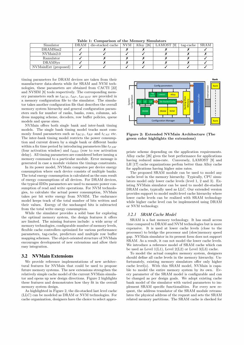
Table 1: Comparison of the Memory SimulatorsSimulator DRAM die-stacked cache NVM Alloy [26] LAMOST [9] tag-cache SRAM

DRAMSim2 3 7 7 7 7 7 3

NVMain2.0 3 3 3 3 7 7 7

Ramulator 3 7 7 7 7 7 3

DRAMSys 3 7 7 7 7 7 3

NVMainExt (proposed) 3 3 3 3 3 3 3

timing parameters for DRAM devices are taken from theirmanufacturer data-sheets while for SRAM and NVM tech-nologies, these parameters are obtained from CACTI [22]and NVSIM [8] tools respectively. The corresponding mem-ory parameters such as tRCD, tRP , tBURST are provided ina memory configuration file to the simulator. The simula-tor takes another configuration file that describes the overallmemory system hierarchy and general configuration param-eters such for number of ranks, banks, rows, columns, ad-dress mapping scheme, decoders, row buffer policies, queuemodels and queue sizes.

NVMain offers both single bank and inter-bank timingmodels. The single bank timing model tracks most com-monly found parameters such as tRCD, tRP and tCAS etc.The inter-bank timing model restricts the power consump-tion and current drawn by a single bank or different bankswithin a fix time period by introducing parameters like tFAW

(four activation window) and tRRD (row to row activationdelay). All timing parameters are considered before issuing amemory command to a particular module. Error message isgenerated in case a module violates the timings constraints.

In its power model, NVMain computes per device energyconsumption where each device consists of multiple banks.The total energy consumption is calculated as the sum resultof energy consumptions of all devices. For DRAM devices,the typical IDDx parameters are used to measure power con-sumption of read and write operations. For NVM technolo-gies, to calculate the actual power consumption, NVMaintakes per bit write energy from NVSIM. The endurancemodel keeps track of the total number of bits written andtheir values. Energy of the unchanged bits is subtractedfrom the total write energy consumption.

While the simulator provides a solid base for exploringthe optimal memory system, the design features it offersare limited. The missing features include: a wide array ofmemory technologies, configurable number of memory levels,flexible cache controllers optimized for various performanceparameters, tag-cache, predictors and multiple row buffermapping schemes. The object-oriented structure of NVMainencourages development of new extensions and allow theireasy integration.

3.2 NVMain ExtensionsWe provide reference implementations of new architec-

tural features for NVMain that could be used to proposefuture memory systems. The new extensions strengthen therelatively simple cache model of the current NVMain simula-tor and opens up new design directions. Figure 2 highlightsthese features and demonstrates how they fit in the overallmemory system design.

As highlighted in Figure 2, the die-stacked last level cache(LLC) can be modeled as DRAM or NVM technologies. Forcache organization, designers have the choice to select appro-

Inte

rco

nn

ect

LAMOST Alloy

Configuration Manager

Syst

em

Co

nfi

gura

tio

n

Config parameters

Bac

kin

g M

ain

M

emo

ry

Mem

ory

Co

ntr

olle

r

Rank

Bank

Bank

SRAM DRAM NVM

L1 L2 L3 Die-Stacked Cache

Tagcache

Figure 2: Extended NVMain Architecture (Thegreen color highlights the extensions)

priate scheme depending on the application requirements.Alloy cache [26] gives the best performance for applicationshaving reduced miss-rate. Conversely, LAMOST [9] andLH [17] cache organizations perfom better than Alloy cachefor applications having higher miss rates.

The proposed SRAM module can be used to model anycache level in the memory hierarchy. Typically, CPU simu-lators model only lower cache levels (level 1, 2 and 3). Ex-isting NVMain simulator can be used to model die-stackedDRAM cache, typically used as LLC. Our extended versionprovides support to model multi-level cache hierarchy wherelower cache levels can be realized with SRAM technologywhile higher cache level can be implemented using DRAMor NVM technology.

3.2.1 SRAM Cache ModelSRAM is a fast memory technology. It has small access

time compared to DRAM and NVM technologies but is moreexpensive. It is used at lower cache levels (close to theprocessor) to bridge the processor and (slow)memory speedgap. NVMain simulator in its present form does not supportSRAM. As a result, it can not model the lower cache levels.We introduce a reference model of SRAM cache which canbe used as Level 1(L1), Level 2(L2) or Level 3(L3) cache.

To model the actual complex memory system, designersshould define all cache levels in the memory hierarchy. Un-fortunately, existing memory simulators offer only highercache level(s). With this SRAM model, NVMain is capa-ble to model the entire memory system by its own. Ev-ery parameter of the SRAM model is configurable and canbe changed as per design goals. We adopt existing cachebank model of the simulator with varied parameters to im-plement SRAM specific functionalities. For every new re-quest, the address translator of the SRAM module retrans-lates the physical address of the request and sets the SRAMrelated memory partitions. The SRAM cache is checked for

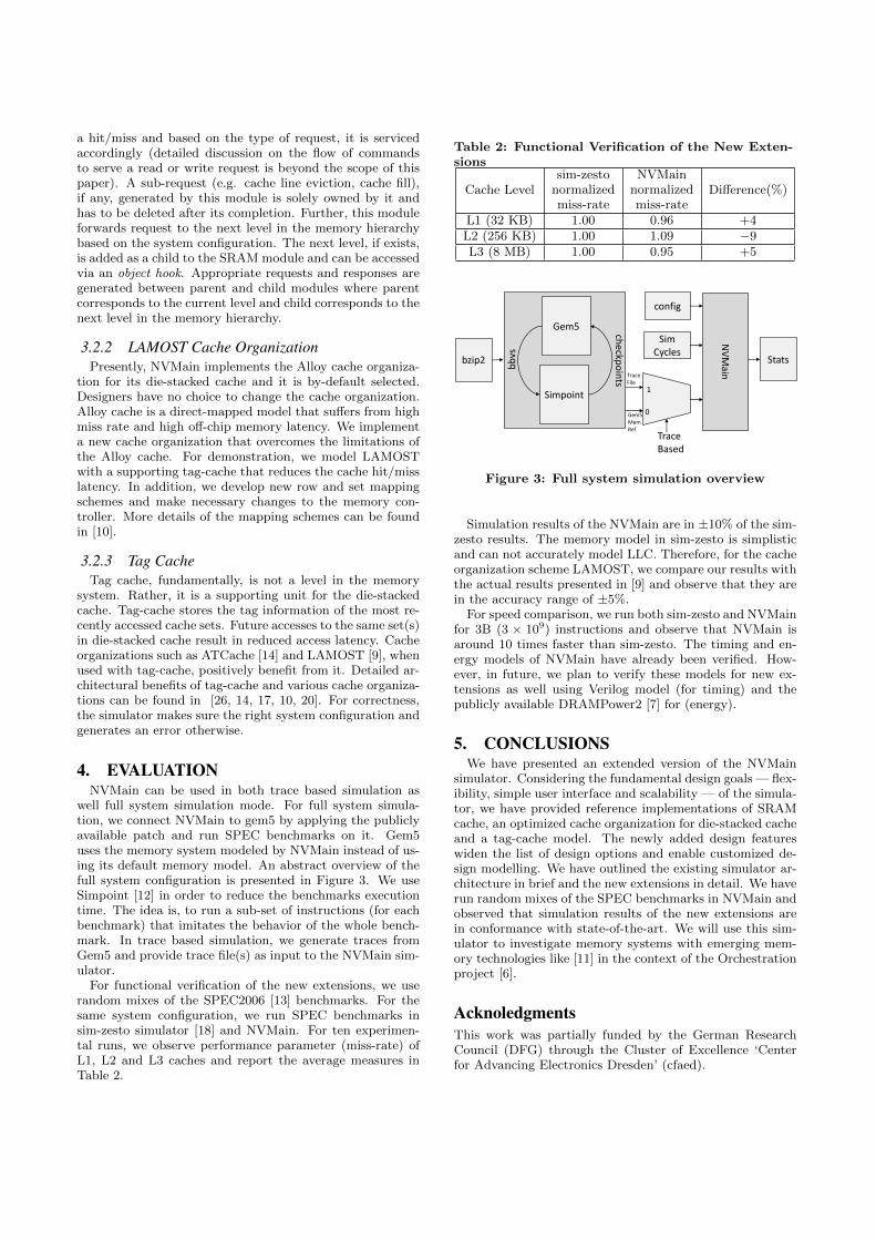
a hit/miss and based on the type of request, it is servicedaccordingly (detailed discussion on the flow of commandsto serve a read or write request is beyond the scope of thispaper). A sub-request (e.g. cache line eviction, cache fill),if any, generated by this module is solely owned by it andhas to be deleted after its completion. Further, this moduleforwards request to the next level in the memory hierarchybased on the system configuration. The next level, if exists,is added as a child to the SRAM module and can be accessedvia an object hook. Appropriate requests and responses aregenerated between parent and child modules where parentcorresponds to the current level and child corresponds to thenext level in the memory hierarchy.

3.2.2 LAMOST Cache OrganizationPresently, NVMain implements the Alloy cache organiza-

tion for its die-stacked cache and it is by-default selected.Designers have no choice to change the cache organization.Alloy cache is a direct-mapped model that suffers from highmiss rate and high off-chip memory latency. We implementa new cache organization that overcomes the limitations ofthe Alloy cache. For demonstration, we model LAMOSTwith a supporting tag-cache that reduces the cache hit/misslatency. In addition, we develop new row and set mappingschemes and make necessary changes to the memory con-troller. More details of the mapping schemes can be foundin [10].

3.2.3 Tag CacheTag cache, fundamentally, is not a level in the memory

system. Rather, it is a supporting unit for the die-stackedcache. Tag-cache stores the tag information of the most re-cently accessed cache sets. Future accesses to the same set(s)in die-stacked cache result in reduced access latency. Cacheorganizations such as ATCache [14] and LAMOST [9], whenused with tag-cache, positively benefit from it. Detailed ar-chitectural benefits of tag-cache and various cache organiza-tions can be found in [26, 14, 17, 10, 20]. For correctness,the simulator makes sure the right system configuration andgenerates an error otherwise.

4. EVALUATIONNVMain can be used in both trace based simulation as

well full system simulation mode. For full system simula-tion, we connect NVMain to gem5 by applying the publiclyavailable patch and run SPEC benchmarks on it. Gem5uses the memory system modeled by NVMain instead of us-ing its default memory model. An abstract overview of thefull system configuration is presented in Figure 3. We useSimpoint [12] in order to reduce the benchmarks executiontime. The idea is, to run a sub-set of instructions (for eachbenchmark) that imitates the behavior of the whole bench-mark. In trace based simulation, we generate traces fromGem5 and provide trace file(s) as input to the NVMain sim-ulator.

For functional verification of the new extensions, we userandom mixes of the SPEC2006 [13] benchmarks. For thesame system configuration, we run SPEC benchmarks insim-zesto simulator [18] and NVMain. For ten experimen-tal runs, we observe performance parameter (miss-rate) ofL1, L2 and L3 caches and report the average measures inTable 2.

Table 2: Functional Verification of the New Exten-sions

Cache Levelsim-zesto

normalizedmiss-rate

NVMainnormalizedmiss-rate

Difference(%)

L1 (32 KB) 1.00 0.96 +4L2 (256 KB) 1.00 1.09 −9L3 (8 MB) 1.00 0.95 +5

NV

Main

Gem5

Simpoint

bb

vs

che

ckpo

ints

config

SimCycles

Stats

Trace File

Gem5MemRef

TraceBased

0

1

bzip2

Figure 3: Full system simulation overview

Simulation results of the NVMain are in ±10% of the sim-zesto results. The memory model in sim-zesto is simplisticand can not accurately model LLC. Therefore, for the cacheorganization scheme LAMOST, we compare our results withthe actual results presented in [9] and observe that they arein the accuracy range of ±5%.

For speed comparison, we run both sim-zesto and NVMainfor 3B (3 × 109) instructions and observe that NVMain isaround 10 times faster than sim-zesto. The timing and en-ergy models of NVMain have already been verified. How-ever, in future, we plan to verify these models for new ex-tensions as well using Verilog model (for timing) and thepublicly available DRAMPower2 [7] for (energy).

5. CONCLUSIONSWe have presented an extended version of the NVMain

simulator. Considering the fundamental design goals — flex-ibility, simple user interface and scalability — of the simula-tor, we have provided reference implementations of SRAMcache, an optimized cache organization for die-stacked cacheand a tag-cache model. The newly added design featureswiden the list of design options and enable customized de-sign modelling. We have outlined the existing simulator ar-chitecture in brief and the new extensions in detail. We haverun random mixes of the SPEC benchmarks in NVMain andobserved that simulation results of the new extensions arein conformance with state-of-the-art. We will use this sim-ulator to investigate memory systems with emerging mem-ory technologies like [11] in the context of the Orchestrationproject [6].

AcknoledgmentsThis work was partially funded by the German ResearchCouncil (DFG) through the Cluster of Excellence ‘Centerfor Advancing Electronics Dresden’ (cfaed).

6. REFERENCES[1] E. Argollo, A. Falcon, P. Faraboschi, M. Monchiero,

and D. Ortega. Cotson: Infrastructure for full systemsimulation. SIGOPS Oper. Syst. Rev., 43(1):52–61,Jan. 2009.

[2] R. Bedicheck. Simnow: Fast platform simulationpurely in software. In Hot Chips 16, 2004.

[3] N. Binkert, B. Beckmann, G. Black, S. K. Reinhardt,A. Saidi, A. Basu, J. Hestness, D. R. Hower,T. Krishna, S. Sardashti, R. Sen, K. Sewell,M. Shoaib, N. Vaish, M. D. Hill, and D. A. Wood. Thegem5 simulator. SIGARCH Comput. Archit. News,39(2):1–7, Aug. 2011.

[4] P. Bohrer, J. Peterson, M. Elnozahy, R. Rajamony,A. Gheith, R. Rockhold, C. Lefurgy, H. Shafi,T. Nakra, R. Simpson, E. Speight, K. Sudeep,E. Van Hensbergen, and L. Zhang. Mambo: A fullsystem simulator for the powerpc architecture.SIGMETRICS Perform. Eval. Rev., 31(4):8–12, Mar.2004.

[5] T. E. Carlson, W. Heirman, and L. Eeckhout. Sniper:Exploring the level of abstraction for scalable andaccurate parallel multi-core simulation. In Proceedingsof 2011 International Conference for HighPerformance Computing, Networking, Storage andAnalysis, SC ’11, pages 52:1–52:12, New York, NY,USA, 2011. ACM.

[6] J. Castrillon, M. Lieber, S. Kluppelholz, M. Volp,N. Asmussen, U. Assmann, F. Baader, C. Baier,G. Fettweis, J. Frohlich, A. Goens, S. Haas, D. Habich,H. Hartig, M. Hasler, I. Huismann, T. Karnagel,S. Karol, A. Kumar, W. Lehner, L. Leuschner, S. Ling,S. Marcker, C. Menard, J. Mey, W. Nagel, B. Nothen,R. Penaloza, M. Raitza, J. Stiller, A. Ungethum,A. Voigt, and S. Wunderlich. A hardware/softwarestack for heterogeneous systems. IEEE Transactionson Multi-Scale Computing Systems, Nov. 2017.

[7] K. Chandrasekar, B. Akesson, and K. Goossens.Improved power modeling of ddr sdrams. InProceedings of the 2011 14th Euromicro Conference onDigital System Design, DSD ’11, pages 99–108,Washington, DC, USA, 2011. IEEE Computer Society.

[8] X. Dong, C. Xu, Y. Xie, and N. P. Jouppi. Nvsim: Acircuit-level performance, energy, and area model foremerging nonvolatile memory. IEEE Transactions onComputer-Aided Design of Integrated Circuits andSystems, 31(7):994–1007, July 2012.

[9] F. Hameed, L. Bauer, and J. Henkel. Simultaneouslyoptimizing dram cache hit latency and miss rate vianovel set mapping policies. In 2013 InternationalConference on Compilers, Architecture and Synthesisfor Embedded Systems (CASES), pages 1–10, Sept2013.

[10] F. Hameed, L. Bauer, and J. Henkel. Architectingon-chip dram cache for simultaneous miss rate andlatency reduction. IEEE Transactions onComputer-Aided Design of Integrated Circuits andSystems, 35(4):651–664, April 2016.

[11] F. Hameed, C. Menard, and J. Castrillon. Efficientstt-ram last-level-cache architecture to replace dramcache. In Proceedings of the International Symposiumon Memory Systems (MemSys’17), MEMSYS ’17,

pages 141–151, New York, NY, USA, Oct. 2017. ACM.

[12] G. HAMERLY. Simpoint 3.0 : Faster and moreflexible program analysis. Workshop on Modeling,Benchmarking and Simulation, 2005, 2005.

[13] J. L. Henning. Spec cpu2006 benchmark descriptions.SIGARCH Comput. Archit. News, 34(4):1–17, Sept.2006.

[14] C.-C. Huang and V. Nagarajan. Atcache: Reducingdram cache latency via a small sram tag cache. InProceedings of the 23rd International Conference onParallel Architectures and Compilation, PACT ’14,pages 51–60, New York, NY, USA, 2014. ACM.

[15] M. Jung, C. Weis, and N. Wehn. Dramsys: A flexibledram subsystem design space exploration framework.IPSJ Transactions on System LSI DesignMethodology, 8:63–74, 2015.

[16] Y. Kim, W. Yang, and O. Mutlu. Ramulator: A fastand extensible dram simulator. IEEE Comput. Archit.Lett., 15(1):45–49, Jan. 2016.

[17] G. Loh and M. D. Hill. Supporting very large dramcaches with compound-access scheduling andmissmap. IEEE Micro, 32(3):70–78, May 2012.

[18] G. H. Loh, S. Subramaniam, and Y. Xie. Zesto: Acycle-level simulator for highly detailedmicroarchitecture exploration. In 2009 IEEEInternational Symposium on Performance Analysis ofSystems and Software, pages 53–64, April 2009.

[19] C. Menard, J. Castrillon, M. Jung, and N. Wehn.System simulation with gem5 and systemc thekeystone for full interoperability. 2017.

[20] J. Meza, J. Chang, H. Yoon, O. Mutlu, andP. Ranganathan. Enabling efficient and scalablehybrid memories using fine-granularity dram cachemanagement. IEEE Computer Architecture Letters,11(2):61–64, July 2012.

[21] J. E. Miller, H. Kasture, G. Kurian, C. Gruenwald,N. Beckmann, C. Celio, J. Eastep, and A. Agarwal.Graphite: A distributed parallel simulator formulticores. In HPCA - 16 2010 The SixteenthInternational Symposium on High-PerformanceComputer Architecture, pages 1–12, Jan 2010.

[22] N. Muralimanohart and N. Balasubramonian,R.and Jouppi. Optimizing NUCA Organizations andWiring Alternatives for Large Caches with CACTI6.0. In Proceedings of the 40th Annual IEEE/ACMInternational Symposium on Microarchitecture(MICRO), pages 3–14, December 2007.

[23] M. Pellauer, M. Adler, M. Kinsy, A. Parashar, andJ. Emer. Hasim: Fpga-based high-detail multicoresimulation using time-division multiplexing. In 2011IEEE 17th International Symposium on HighPerformance Computer Architecture, pages 406–417,Feb 2011.

[24] M. Poremba and Y. Xie. Nvmain: Anarchitectural-level main memory simulator foremerging non-volatile memories. In 2012 IEEEComputer Society Annual Symposium on VLSI, pages392–397, Aug 2012.

[25] M. Poremba, T. Zhang, and Y. Xie. Nvmain 2.0: Auser-friendly memory simulator to model(non-)volatile memory systems. IEEE ComputerArchitecture Letters, 14(2):140–143, July 2015.

[26] M. K. Qureshi and G. H. Loh. Fundamental latencytrade-off in architecting dram caches: Outperformingimpractical sram-tags with a simple and practicaldesign. In Proceedings of the 2012 45th AnnualIEEE/ACM International Symposium onMicroarchitecture, MICRO-45, pages 235–246,Washington, DC, USA, 2012. IEEE Computer Society.

[27] P. Rosenfeld, E. Cooper-Balis, and B. Jacob.Dramsim2: A cycle accurate memory systemsimulator. IEEE Comput. Archit. Lett., 10(1):16–19,Jan. 2011.

[28] J. Stevens, P. Tschirhart, C. Mu-Tien, I. Bhati,P. Enns, J. Greensky, Z. Chisti, L. Shih-Lien, and

B. Jacob. An integrated simulation infrastructure forthe entire memory hierarchy: Cache , dram, nonvolatile memory, and disk. Intel Technology Journal,17(1):184 – 200, 2013.

[29] D. Wang, B. Ganesh, N. Tuaycharoen, K. Baynes,A. Jaleel, and B. Jacob. Dramsim: A memory systemsimulator. SIGARCH Comput. Archit. News,33(4):100–107, Nov. 2005.

[30] K. Wang, Y. Zhang, H. Wang, and X. Shen.Parallelization of ibm mambo system simulator infunctional modes. SIGOPS Oper. Syst. Rev.,

42(1):71–76, Jan. 2008.

LXVI

Work in progress paper : A FaultInjection Platform for Early-StageReliability Assessment

LXVII

A Fault Injection Platform for Early-Stage Reliability AssessmentAlexandre CHABOTCEA, LIST - LAMIH

Software Reliability and Security LaboratoryP.C. 174, Gif-sur-Yvette, 91191, France

alexandre.chabot@cea.fr

Reda NOUACERCEA, LIST

Software Reliability and Security LaboratoryP.C. 174, Gif-sur-Yvette, 91191, France

reda.nouacert@cea.fr

Ihsen ALOUANILAMIH

University of ValenciennesValenciennes, 59300, France

ihsen.alouani@univ-valenciennes.fr

Smail NIARLAMIH

University of ValenciennesValenciennes, 59300, France

smail.niar@univ-valenciennes.fr

ABSTRACTWith new integration rates, embedded systems sensitivity to envi-ronmental conditions has increased drastically. Thus, presentingreliable architectures is one of the major concerns for designers.During the development life-cycle of fault-tolerant computer sys-tems, the dependability insurance is a complex and critical task.This work in progress paper presents a technique for reliabilityevaluation of embedded systems at early-stage by demonstratingthe functionality and usage of simulation based fault injection. Theproposed technique takes into account both the environmentalconditions and the behavior of the application. Our results bringa flexible fault injection methodology and show its usability forreliability evaluation during simulation phase.

KEYWORDSFault injection, environmental conditions, application behavior,reliability, virtual prototypeACM Reference Format:Alexandre CHABOT, Reda NOUACER, Ihsen ALOUANI, and Smail NIAR.2018. A Fault Injection Platform for Early-Stage Reliability Assessment. InProceedings of HIPEAC RAPIDO Conference (RAPIDO’18). ACM, New York,NY, USA, 6 pages. https://doi.org/10.1145/nnnnnnn.nnnnnnn

1 INTRODUCTIONElectronics are more and more present on our daily life. In fact,smart and connected systems are expected to be present practicallyeverywhere in the future decade. This trend is made possible by theprogress manufacturers and designers performed towards provid-ing high performance platforms. However, this performance racehas led to a degradation in embedded systems reliability. In fact,the reliability is a direct reflection of systems sensitivity to tran-sient errors as well as to aging. Soft errors are caused by transientevents that corrupt sequential and combinational elements andtheir impact is increasing dramatically in mainstream computingsystems. Therefore, robustness techniques have been proposed toreach acceptable reliability levels. One of the hardware techniquesconsists of separating memory cells accessed by the same addressto avoid multiple bit flips for the same stored word [10]. We can

RAPIDO’18, January 2018, Manchester, UK2018. ACM ISBN 978-x-xxxx-xxxx-x/YY/MM. . . $15.00https://doi.org/10.1145/nnnnnnn.nnnnnnn

also cite the well-known error correcting code memory that is acomputer data storage able to detect single bit flip. At softwarelevel, techniques such as task redundancy and the work of Huanget al. [14] on scheduling algorithms. Finally, CLEAR project [8]have compared techniques at different system layers.

The evaluation of embedded systems reliability is a complex taskand different techniques are used during different developmentsteps. Usually, reliability is linked to hardware manufacturing pro-cess and environmental conditions. However, having implementedrobustness techniques at different system levels, it appears impor-tant to take it into account while evaluating the system reliabilityto avoid excessive design margins.

In this paper, we focus on transient errors and especially soft er-rors. To evaluate the system reliability, we propose a fault injectionmodel that takes into account all parameters impacting reliability.In addition, our model takes into account the link between the ap-plication behavior and the fluctuation of the memory temperature,this link is exhibited in Section 3.1.2.

The rest of this work in progress paper is organized as follows.In the state of the art, Section 2, we discuss how fault injectionassociated to virtual platforms helps to ensure the correct function-ing of critical systems. Then, in the third Section, we present ourfault injection model. In the fourth Section, we discuss the evalua-tion of the proposed approach using UNISIM-VP [18] simulationenvironment and illustrate its flexibility by implementing some as-pects of FIDES standard [11]. Finally, we present some preliminaryexperimental results.

2 STATE OF THE ARTIn the domain of reliable embedded system design, many techniqueshave been considered to measure the robustness of an architecture.We can list here after the main ones:

• Analytical models: this technique can be used in the earlyphases of the design. It uses high level modeling of the systemand approximations to determine the most critical functionsin terms of reliability. We can cite the work done in SOPHIA[4]

• Prototyping: this method is often the last step of the devel-opment and the goal is to realize as less as prototypes aspossible as it is a very expensive step [21].

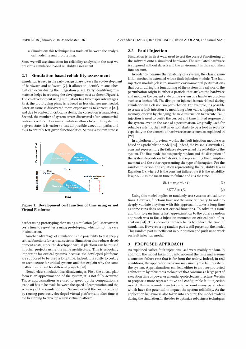
RAPIDO’18, January 2018, Manchester, UK Alexandre CHABOT, Reda NOUACER, Ihsen ALOUANI, and Smail NIAR

• Simulation: this technique is a trade-off between the analyti-cal modeling and prototyping.

Since we will use simulation for reliability analysis, in the next wepresent a simulation based reliability assessment.

2.1 Simulation based reliability assessmentSimulation is used in the early design phase to ease the co-developmentof hardware and software [7]. It allows to identify mismatchesthat can occur during the integration phase. Early identifying mis-matches helps in reducing the development cost as shown Figure 1.The co-development using simulation has two major advantages.First, the prototyping phase is reduced as less changes are needed.Later an issue is discovered more expensive is to correct it [21],and due to context of critical systems, the correction is mandatory.Second, the number of system errors discovered after commercial-ization is reduced. Because simulation allows to put the system ina given state, it is easier to test all possible execution paths andthus to entirely test given functionalities. Setting a system state is

Figure 1: Development cost function of time using or notVirtual Platforms

harder using prototyping than using simulation [23]. Moreover, itcosts time to repeat tests using prototyping, which is not the casein simulation.

Another advantage of simulation is the possibility to test deeplycritical functions for critical systems. Simulation also reduces devel-opment costs, since the developed virtual platform can be reusedin other projects using the same architecture. This is especiallyimportant for critical systems, because the developed platformsare supposed to be used a long time. Indeed, it is costly to certifyan architecture for critical systems and that explain why the sameplatform is reused for different projects [20].

Nonetheless simulation has disadvantages. First, the virtual plat-form is an approximation of the system, it is not fully accurate.Those approximations are used to speed up the computation, atrade-off has to be made between the speed of computation and theaccuracy of the simulation run. Second, even if the cost is reducedby reusing previously developed virtual platforms, it takes time atthe beginning to develop a new virtual platform.

2.2 Fault InjectionSimulation is, in first way, used to test the correct functioning ofthe software onto a simulated hardware. The simulated hardwareis supposed without defects and the environment is thus not takeninto account.

In order to measure the reliability of a system, the classic simu-lation method is extended with a fault injection module. The faultinjection module job is to simulate environmental perturbationsthat occur during the functioning of the system. In real world, theperturbation origin is either a particle that strikes the hardwareand modifies the current state of the system or a hardware problemsuch as a latches fail. The disruption injected is materialized duringsimulation by a classic run perturbation. For example, it’s possibleto create a fault injection by modifying a bus value, flipping a bit inmemory, or even by changing the next instruction to execute. Faultinjection is used to verify the correct and time limited response ofthe system, even in the case of a perturbation. Originally used forreliable systems, the fault injection starts to be a tool in securityespecially in the context of hardware attacks such as explained in[22].

In a plethora of previous works, the fault injection module wasbased on a probabilistic model [24]. Indeed, the Poison’s lawwith a λconstant representing the failure rate, governed the reliability of thesystem. The first model is thus purely random and the disruption ofthe system depends on two draws: one representing the disruptionmoment and the other representing the type of disruption. For therandom injection, the equation representing the reliability law isEquation (1), where λ is the constant failure rate R is the reliabilitylaw,MTTF is the mean time to failure and t is the time.

R(t) = exp(−λ ∗ t) (1)

MTTF = 1/λ (2)Using this model implies to randomly test systems critical func-

tions. However, functions have not the same criticality. In order todeeply validate a system with this approach it takes a long timeas some runs does not test critical functions. To solve this issueand thus to gain time, a first approximation to the purely randomapproach was to focus injection moments on critical path of ex-ecution [24]. This second approach helps to reduce the time ofsimulation. However, a big random part is still present in the model.This random part is inefficient in our opinion and push us to workon fault injection model.

3 PROPOSED APPROACHAs explained earlier, fault injections used were mainly random. Inaddition, the model takes only into account the time and assumea constant failure rate that is far from the reality. Indeed, in realconditions, the application behavior may modify the failure rate ofthe system. Approximations can lead either to an over-protectedarchitecture by robustness techniques that consumes a large part ofexecution time or power or an under-protected architecture.We aimto propose a more representative and configurable fault injectionmodel. This new model can take into account many parameterswhich have the potential to impact the system reliability. As theapplication behavior is also taken into account, the model evolvesduring the simulation. In the idea to optimize robustness techniques

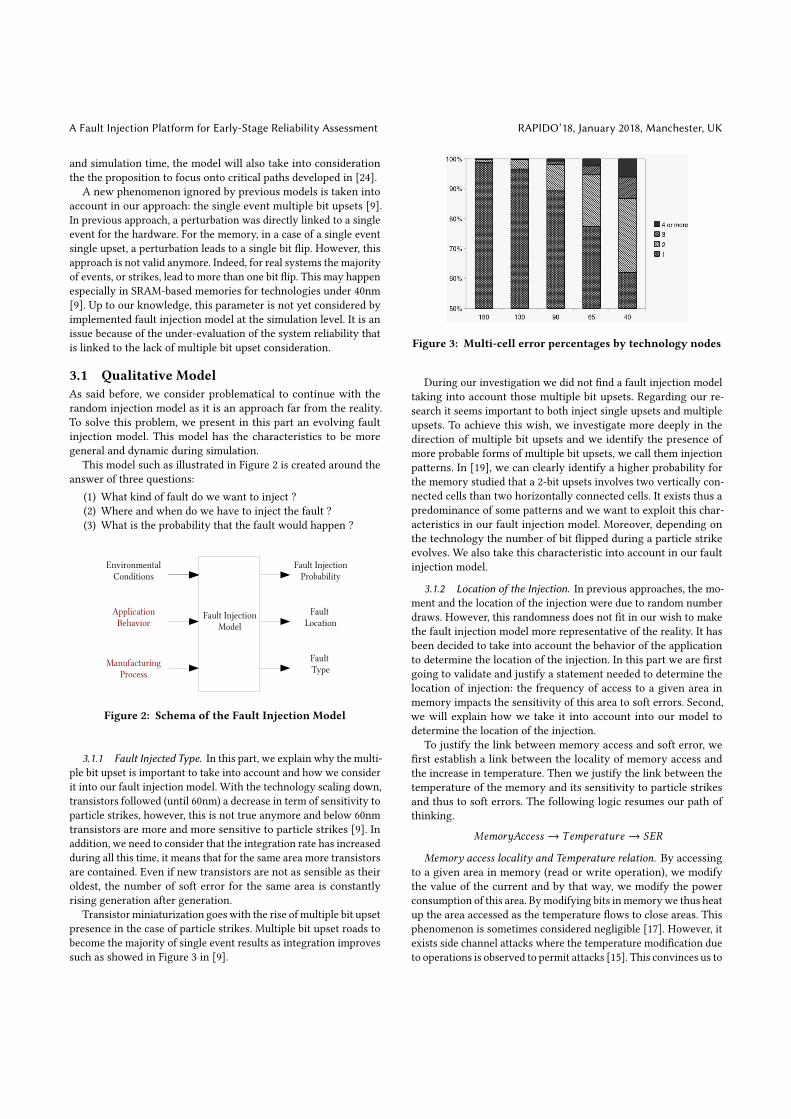
A Fault Injection Platform for Early-Stage Reliability Assessment RAPIDO’18, January 2018, Manchester, UK

and simulation time, the model will also take into considerationthe the proposition to focus onto critical paths developed in [24].

A new phenomenon ignored by previous models is taken intoaccount in our approach: the single event multiple bit upsets [9].In previous approach, a perturbation was directly linked to a singleevent for the hardware. For the memory, in a case of a single eventsingle upset, a perturbation leads to a single bit flip. However, thisapproach is not valid anymore. Indeed, for real systems the majorityof events, or strikes, lead to more than one bit flip. This may happenespecially in SRAM-based memories for technologies under 40nm[9]. Up to our knowledge, this parameter is not yet considered byimplemented fault injection model at the simulation level. It is anissue because of the under-evaluation of the system reliability thatis linked to the lack of multiple bit upset consideration.

3.1 Qualitative ModelAs said before, we consider problematical to continue with therandom injection model as it is an approach far from the reality.To solve this problem, we present in this part an evolving faultinjection model. This model has the characteristics to be moregeneral and dynamic during simulation.

This model such as illustrated in Figure 2 is created around theanswer of three questions:

(1) What kind of fault do we want to inject ?(2) Where and when do we have to inject the fault ?(3) What is the probability that the fault would happen ?

Fault Injection Model

Environmental Conditions

Application Behavior

Manufacturing Process

Fault Injection Probability

Fault Location

Fault Type

Figure 2: Schema of the Fault Injection Model

3.1.1 Fault Injected Type. In this part, we explain why the multi-ple bit upset is important to take into account and how we considerit into our fault injection model. With the technology scaling down,transistors followed (until 60nm) a decrease in term of sensitivity toparticle strikes, however, this is not true anymore and below 60nmtransistors are more and more sensitive to particle strikes [9]. Inaddition, we need to consider that the integration rate has increasedduring all this time, it means that for the same area more transistorsare contained. Even if new transistors are not as sensible as theiroldest, the number of soft error for the same area is constantlyrising generation after generation.

Transistor miniaturization goes with the rise of multiple bit upsetpresence in the case of particle strikes. Multiple bit upset roads tobecome the majority of single event results as integration improvessuch as showed in Figure 3 in [9].

Figure 3: Multi-cell error percentages by technology nodes

During our investigation we did not find a fault injection modeltaking into account those multiple bit upsets. Regarding our re-search it seems important to both inject single upsets and multipleupsets. To achieve this wish, we investigate more deeply in thedirection of multiple bit upsets and we identify the presence ofmore probable forms of multiple bit upsets, we call them injectionpatterns. In [19], we can clearly identify a higher probability forthe memory studied that a 2-bit upsets involves two vertically con-nected cells than two horizontally connected cells. It exists thus apredominance of some patterns and we want to exploit this char-acteristics in our fault injection model. Moreover, depending onthe technology the number of bit flipped during a particle strikeevolves. We also take this characteristic into account in our faultinjection model.

3.1.2 Location of the Injection. In previous approaches, the mo-ment and the location of the injection were due to random numberdraws. However, this randomness does not fit in our wish to makethe fault injection model more representative of the reality. It hasbeen decided to take into account the behavior of the applicationto determine the location of the injection. In this part we are firstgoing to validate and justify a statement needed to determine thelocation of injection: the frequency of access to a given area inmemory impacts the sensitivity of this area to soft errors. Second,we will explain how we take it into account into our model todetermine the location of the injection.

To justify the link between memory access and soft error, wefirst establish a link between the locality of memory access andthe increase in temperature. Then we justify the link between thetemperature of the memory and its sensitivity to particle strikesand thus to soft errors. The following logic resumes our path ofthinking.

MemoryAccess → Temperature → SER

Memory access locality and Temperature relation. By accessingto a given area in memory (read or write operation), we modifythe value of the current and by that way, we modify the powerconsumption of this area. Bymodifying bits inmemorywe thus heatup the area accessed as the temperature flows to close areas. Thisphenomenon is sometimes considered negligible [17]. However, itexists side channel attacks where the temperature modification dueto operations is observed to permit attacks [15]. This convinces us to

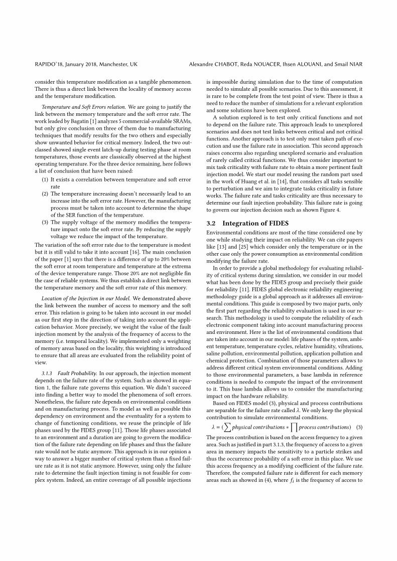
RAPIDO’18, January 2018, Manchester, UK Alexandre CHABOT, Reda NOUACER, Ihsen ALOUANI, and Smail NIAR

consider this temperature modification as a tangible phenomenon.There is thus a direct link between the locality of memory accessand the temperature modification.

Temperature and Soft Errors relation. We are going to justify thelink between the memory temperature and the soft error rate. Thework leaded by Bagatin [1] analyzes 5 commercial-available SRAMs,but only give conclusion on three of them due to manufacturingtechniques that modify results for the two others and especiallyshow unwanted behavior for critical memory. Indeed, the two out-classed showed single event latch-up during testing phase at roomtemperatures, those events are classically observed at the highestoperating temperature. For the three device remaining, here followsa list of conclusion that have been raised:

(1) It exists a correlation between temperature and soft errorrate

(2) The temperature increasing doesn’t necessarily lead to anincrease into the soft error rate. However, the manufacturingprocess must be taken into account to determine the shapeof the SER function of the temperature.

(3) The supply voltage of the memory modifies the tempera-ture impact onto the soft error rate. By reducing the supplyvoltage we reduce the impact of the temperature.

The variation of the soft error rate due to the temperature is modestbut it is still valid to take it into account [16]. The main conclusionof the paper [1] says that there is a difference of up to 20% betweenthe soft error at room temperature and temperature at the extremaof the device temperature range. Those 20% are not negligible finthe case of reliable systems. We thus establish a direct link betweenthe temperature memory and the soft error rate of this memory.

Location of the Injection in our Model. We demonstrated abovethe link between the number of access to memory and the softerror. This relation is going to be taken into account in our modelas our first step in the direction of taking into account the appli-cation behavior. More precisely, we weight the value of the faultinjection moment by the analysis of the frequency of access to thememory (i.e. temporal locality). We implemented only a weightingof memory areas based on the locality, this weighting is introducedto ensure that all areas are evaluated from the reliability point ofview.

3.1.3 Fault Probability. In our approach, the injection momentdepends on the failure rate of the system. Such as showed in equa-tion 1, the failure rate governs this equation. We didn’t succeedinto finding a better way to model the phenomena of soft errors.Nonetheless, the failure rate depends on environmental conditionsand on manufacturing process. To model as well as possible thisdependency on environment and the eventuality for a system tochange of functioning conditions, we reuse the principle of lifephases used by the FIDES group [11]. Those life phases associatedto an environment and a duration are going to govern the modifica-tion of the failure rate depending on life phases and thus the failurerate would not be static anymore. This approach is in our opinion away to answer a bigger number of critical system than a fixed fail-ure rate as it is not static anymore. However, using only the failurerate to determine the fault injection timing is not feasible for com-plex system. Indeed, an entire coverage of all possible injections

is impossible during simulation due to the time of computationneeded to simulate all possible scenarios. Due to this assessment, itis rare to be complete from the test point of view. There is thus aneed to reduce the number of simulations for a relevant explorationand some solutions have been explored.

A solution explored is to test only critical functions and notto depend on the failure rate. This approach leads to unexploredscenarios and does not test links between critical and not criticalfunctions. Another approach is to test only most taken path of exe-cution and use the failure rate in association. This second approachraises concerns also regarding unexplored scenario and evaluationof rarely called critical functions. We thus consider important tomix task criticality with failure rate to obtain a more pertinent faultinjection model. We start our model reusing the random part usedin the work of Huang et al. in [14], that considers all tasks sensibleto perturbation and we aim to integrate tasks criticality in futureworks. The failure rate and tasks criticality are thus necessary todetermine our fault injection probability. This failure rate is goingto govern our injection decision such as shown Figure 4.

3.2 Integration of FIDESEnvironmental conditions are most of the time considered one byone while studying their impact on reliability. We can cite paperslike [13] and [25] which consider only the temperature or in theother case only the power consumption as environmental conditionmodifying the failure rate.

In order to provide a global methodology for evaluating reliabil-ity of critical systems during simulation, we consider in our modelwhat has been done by the FIDES group and precisely their guidefor reliability [11]. FIDES global electronic reliability engineeringmethodology guide is a global approach as it addresses all environ-mental conditions. This guide is composed by two major parts, onlythe first part regarding the reliability evaluation is used in our re-search. This methodology is used to compute the reliability of eachelectronic component taking into account manufacturing processand environment. Here is the list of environmental conditions thatare taken into account in our model: life phases of the system, ambi-ent temperature, temperature cycles, relative humidity, vibrations,saline pollution, environmental pollution, application pollution andchemical protection. Combination of those parameters allows toaddress different critical system environmental conditions. Addingto those environmental parameters, a base lambda in referenceconditions is needed to compute the impact of the environmentto it. This base lambda allows us to consider the manufacturingimpact on the hardware reliability.

Based on FIDES model (3), physical and process contributionsare separable for the failure rate called λ. We only keep the physicalcontribution to simulate environmental conditions.λ = (

∑physical contributions ∗

∏process contributions) (3)

The process contribution is based on the access frequency to a givenarea. Such as justified in part 3.1.3, the frequency of access to a givenarea in memory impacts the sensitivity to a particle strikes andthus the occurrence probability of a soft error in this place. We usethis access frequency as a modifying coefficient of the failure rate.Therefore, the computed failure rate is different for each memoryareas such as showed in (4), where fi is the frequency of access to

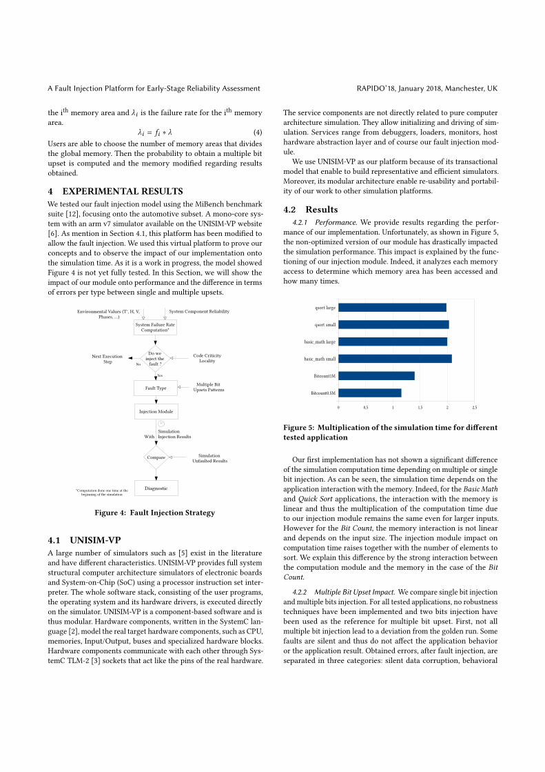
A Fault Injection Platform for Early-Stage Reliability Assessment RAPIDO’18, January 2018, Manchester, UK

the ith memory area and λi is the failure rate for the ith memoryarea.

λi = fi ∗ λ (4)Users are able to choose the number of memory areas that dividesthe global memory. Then the probability to obtain a multiple bitupset is computed and the memory modified regarding resultsobtained.

4 EXPERIMENTAL RESULTSWe tested our fault injection model using the MiBench benchmarksuite [12], focusing onto the automotive subset. A mono-core sys-tem with an arm v7 simulator available on the UNISIM-VP website[6]. As mention in Section 4.1, this platform has been modified toallow the fault injection. We used this virtual platform to prove ourconcepts and to observe the impact of our implementation ontothe simulation time. As it is a work in progress, the model showedFigure 4 is not yet fully tested. In this Section, we will show theimpact of our module onto performance and the difference in termsof errors per type between single and multiple upsets.

System Failure RateComputation*

Fault Type

Injection Module

Compare Simulation Unfaulted Results

Multiple Bit Upsets Patterns

Diagnostic

Simulation With Injection Results

*Computation done one time at the beginning of the simulation

Yes

No

Code CriticityLocality

System Component ReliabilityEnvironmental Values (T°, H, V, Phases, ...)

Do we inject the

fault ?Next Execution

Step

Figure 4: Fault Injection Strategy

4.1 UNISIM-VPA large number of simulators such as [5] exist in the literatureand have different characteristics. UNISIM-VP provides full systemstructural computer architecture simulators of electronic boardsand System-on-Chip (SoC) using a processor instruction set inter-preter. The whole software stack, consisting of the user programs,the operating system and its hardware drivers, is executed directlyon the simulator. UNISIM-VP is a component-based software and isthus modular. Hardware components, written in the SystemC lan-guage [2], model the real target hardware components, such as CPU,memories, Input/Output, buses and specialized hardware blocks.Hardware components communicate with each other through Sys-temC TLM-2 [3] sockets that act like the pins of the real hardware.

The service components are not directly related to pure computerarchitecture simulation. They allow initializing and driving of sim-ulation. Services range from debuggers, loaders, monitors, hosthardware abstraction layer and of course our fault injection mod-ule.

We use UNISIM-VP as our platform because of its transactionalmodel that enable to build representative and efficient simulators.Moreover, its modular architecture enable re-usability and portabil-ity of our work to other simulation platforms.

4.2 Results4.2.1 Performance. We provide results regarding the perfor-

mance of our implementation. Unfortunately, as shown in Figure 5,the non-optimized version of our module has drastically impactedthe simulation performance. This impact is explained by the func-tioning of our injection module. Indeed, it analyzes each memoryaccess to determine which memory area has been accessed andhow many times.

qsort_large

qsort_small

basicmath_small

basicmath_large

Bitcount0.5M

Bitcount1M

0 1 2 3 4 5 6 7 8

Bitcount0.5M

Bitcount1M

basic_math small

basic_math large

qsort small

qsort large

0 0,5 1 1,5 2 2,5

Figure 5: Multiplication of the simulation time for differenttested application

Our first implementation has not shown a significant differenceof the simulation computation time depending on multiple or singlebit injection. As can be seen, the simulation time depends on theapplication interaction with the memory. Indeed, for the Basic Mathand Quick Sort applications, the interaction with the memory islinear and thus the multiplication of the computation time dueto our injection module remains the same even for larger inputs.However for the Bit Count, the memory interaction is not linearand depends on the input size. The injection module impact oncomputation time raises together with the number of elements tosort. We explain this difference by the strong interaction betweenthe computation module and the memory in the case of the BitCount.

4.2.2 Multiple Bit Upset Impact. We compare single bit injectionand multiple bits injection. For all tested applications, no robustnesstechniques have been implemented and two bits injection havebeen used as the reference for multiple bit upset. First, not allmultiple bit injection lead to a deviation from the golden run. Somefaults are silent and thus do not affect the application behavioror the application result. Obtained errors, after fault injection, areseparated in three categories: silent data corruption, behavioral

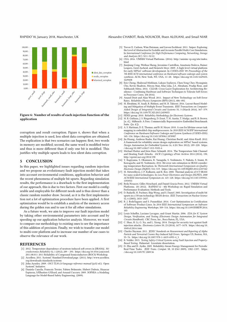
RAPIDO’18, January 2018, Manchester, UK Alexandre CHABOT, Reda NOUACER, Ihsen ALOUANI, and Smail NIAR

qsort_small

qsort_large

basicmath_small_mbu

basicmath_small

basicmath_large_mbu

basicmath_large

0,00%

10,00%

20,00%

30,00%

40,00%

50,00%

60,00%

70,00%

80,00%

90,00%100,00%

silent_data_corruptionresults_corruptionbehavioral_corruption

Figure 6: Number of results of each injection function of theapplication

corruption and result corruption. Figure 6, shows that when amultiple injection is used, less silent data corruption are obtained.The explication is that two scenarios can happen: first, two wordsin memory are modified; second, the same word is modified twiceand thus is more different than if only one bit is modified. Thisjustifies why multiple upsets leads to less silent data corruption.

5 CONCLUSIONIn this paper, we highlighted issues regarding random injectionand we propose an evolutionary fault injection model that takesinto account environmental conditions, application behavior andthe recent phenomena of multiple bit upsets. Regarding simulationresults, the performance is a drawback to the first implementationof our approach, this is due to two factors. First our model is config-urable and employable for different needs and is thus slower than aclassic random number draw. Second, as it is the first implementa-tion not a lot of optimization procedure have been applied. A firstoptimization would be to establish a analysis of the memory accessduring the golden run and to use it for all other simulations.

As a future work, we aim to improve our fault injection modelby taking other environmental parameters into account and byspeeding up our application behavior analysis. Moreover, we wantto compare our methodology to existing ones to see the importanceof this addition of precision. Finally, we wish to transfer our modelto multi-core platform and to increase our number of use cases toobserve the relevance of our work.

REFERENCES[1] 2012. Temperature dependence of neutron-induced soft errors in {SRAMs}. Mi-

croelectronics Reliability 52, 1 (2012), 289 – 293. https://doi.org/10.1016/j.microrel.2011.08.011 2011 Reliability of Compound Semiconductors (ROCS) Workshop.

[2] Accellera. 2011. SystemC Standard Download page. (2011). http://www.accellera.org/downloads/standards/systemc

[3] John Aynsley. 2009. OSCI TLM-2.0 language reference manual (ja32 ed.). OpenSystemC Initiative.

[4] Daniela Cancila, Francois Terrier, Fabien Belmonte, Hubert Dubois, HuascarEspinoza, SÃľbastien GÃľrard, and Arnaud Cuccuru. 2009. SOPHIA: a ModelingLanguage for Model-Based Safety Engineering. (2009).

[5] Trevor E. Carlson, Wim Heirman, and Lieven Eeckhout. 2011. Sniper: Exploringthe Level of Abstraction for Scalable andAccurate ParallelMulti-Core Simulations.In International Conference for High Performance Computing, Networking, Storageand Analysis (SC). 52:1–52:12.

[6] CEA. 2016. UNISIM Virtual Platforms. (2016). http://unisim-vp.org/site/index.html

[7] Jianjiang Ceng, Weihua Sheng, Jeronimo Castrillon, Anastasia Stulova, RainerLeupers, Gerd Ascheid, and Heinrich Meyr. 2009. A high-level virtual platformfor early MPSoC software development. In CODES+ISSS ’09: Proceedings of the7th IEEE/ACM international conference on Hardware/software codesign and systemsynthesis. ACM, New York, NY, USA, 11–20. https://doi.org/10.1145/1629435.1629438

[8] Eric Cheng, Shahrzad Mirkhani, Lukasz Szafaryn, Chen-Yong Cher, HyungminCho, Kevin Skadron, Mircea Stan, Klas Lilja, J.A. Abraham, Pradip Bose, andSubhasish Mitra. 2016. CLEAR: Cross-Layer Exploration for Architecting Re-silience - Combining Hardware and Software Techniques to Tolerate Soft Errorsin Processor Cores. (04 2016).

[9] Anand Dixit and Alan Wood. 2011. Impact of New Technology on Soft ErrorRates. Reliability Physics Symposim (IRPS) (2011), 486–492.

[10] M. Ebrahimi, H. Asadi, R. Bishnoi, and M. B. Tahoori. 2016. Layout-Based Model-ing and Mitigation of Multiple Event Transients. IEEE Transactions on Computer-Aided Design of Integrated Circuits and Systems 35, 3 (March 2016), 367–379.https://doi.org/10.1109/TCAD.2015.2459053

[11] FIDES group. 2010. Reliability Methodology for Electronic Systems.[12] M. R. Guthaus, J. S. Ringenberg, D. Ernst, T. M. Austin, T. Mudge, and R. B. Brown.

[n. d.]. MiBench: A Free, Commercially Representative Embedded BenchmarkSuite. ([n. d.]).

[13] A. S. Hartman, D. E. Thomas, and B. H. Meyer. 2010. A case for lifetime-aware taskmapping in embedded chip multiprocessors. In 2010 IEEE/ACM/IFIP InternationalConference on Hardware/Software Codesign and System Synthesis (CODES+ISSS).145–154. https://doi.org/10.1145/1878961.1878987

[14] Jia Huang, Andreas Raabe, Kai Huang, Christian Buckl, and Alois Knoll. 2012.A framework for reliability-aware design exploration on MPSoC based systems.Design Automation for Embedded Systems 16, 4 (01 Nov 2012), 189–220. https://doi.org/10.1007/s10617-013-9105-6

[15] Michael Hutter and Jörn-Marc Schmidt. 2014. The Temperature Side Channeland Heating Fault Attacks. IACR Cryptology ePrint Archive 2014 (2014), 190.http://eprint.iacr.org/2014/190

[16] Y. Kagiyama, S. Okumura, K. Yanagida, S. Yoshimoto, Y. Nakata, S. Izumi, H.Kawaguchi, and M. Yoshimoto. 2012. Bit error rate estimation in SRAM consider-ing temperature fluctuation. In Thirteenth International Symposium on QualityElectronic Design (ISQED). 516–519. https://doi.org/10.1109/ISQED.2012.6187542

[17] M. Meterelliyoz, J. P. Kulkarni, and K. Roy. 2008. Thermal analysis of 8-T SRAMfor nano-scaled technologies. In Low Power Electronics and Design (ISLPED), 2008ACM/IEEE International Symposium on. 123–128. https://doi.org/10.1145/1393921.1393953

[18] Reda Nouacer, Gilles Mouchard, and Daniel Gracia-Perez. 2012. UNISIM VirtualPlatforms. (01 2012). RAPIDO’12 - 4th Workshop on: Rapid Simulation andPerformance Evaluation: Methods and Tools.

[19] D. Radaelli, H. Puchner, Skip Wong, and S. Daniel. 2005. Investigation of multi-bitupsets in a 150 nm technology SRAM device. IEEE Transactions on Nuclear Science52, 6 (2005), 2433–2437.

[20] R. J. RodrÃŋguez and S. Punnekkat. 2014. Cost Optimisation in Certificationof Software Product Lines. In 2014 IEEE International Symposium on SoftwareReliability Engineering Workshops. 509–514. https://doi.org/10.1109/ISSREW.2014.103

[21] Louis Scheffer, Luciano Lavagno, and Grant Martin. 2006. EDA for IC SystemDesign, Verification, and Testing (Electronic Design Automation for IntegratedCircuits Handbook). CRC Press, Inc., Boca Raton, FL, USA.

[22] C. Shao, H. Li, G. Xu, and L. Xiong. 2014. Design for security test against faultinjection attacks. Electronics Letters 50, 23 (2014), 1677–1678. https://doi.org/10.1049/el.2014.1666

[23] Charles Slayman. 2011. JEDEC Standards on Measurement and Reporting of AlphaParticle and Terrestrial Cosmic Ray Induced Soft Errors. Springer US, Boston, MA,55–76. https://doi.org/10.1007/978-1-4419-6993-4_3

[24] B. Vedder. 2015. Testing Safety-Critical Systems using Fault Injection and Property-Based Testing. Halmstad. Licentiate dissertation.

[25] D. Zhu and H. Aydin. 2009. Reliability-Aware Energy Management for PeriodicReal-Time Tasks. IEEE Trans. Comput. 58, 10 (Oct 2009), 1382–1397. https://doi.org/10.1109/TC.2009.56