Embed Size (px)
Citation preview
Alan Clements Computer Organization and Architecture: Themes and Variations, 1st Edition
© 2014 Cengage Learning Engineering. All Rights Reserved. Computer History – An Overview Page 1
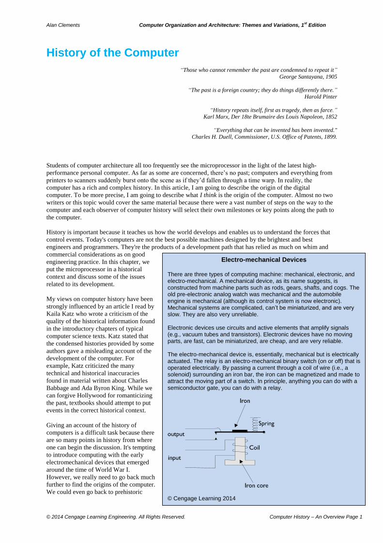
Electro-mechanical Devices There are three types of computing machine: mechanical, electronic, and electro-mechanical. A mechanical device, as its name suggests, is constructed from machine parts such as rods, gears, shafts, and cogs. The old pre-electronic analog watch was mechanical and the automobile engine is mechanical (although its control system is now electronic). Mechanical systems are complicated, can’t be miniaturized, and are very slow. They are also very unreliable. Electronic devices use circuits and active elements that amplify signals (e.g., vacuum tubes and transistors). Electronic devices have no moving parts, are fast, can be miniaturized, are cheap, and are very reliable. The electro-mechanical device is, essentially, mechanical but is electrically actuated. The relay is an electro-mechanical binary switch (on or off) that is operated electrically. By passing a current through a coil of wire (i.e., a solenoid) surrounding an iron bar, the iron can be magnetized and made to attract the moving part of a switch. In principle, anything you can do with a semiconductor gate, you can do with a relay.
© Cengage Learning 2014
History of the Computer
“Those who cannot remember the past are condemned to repeat it”
George Santayana, 1905
“The past is a foreign country; they do things differently there.”
Harold Pinter
“History repeats itself, first as tragedy, then as farce.”
Karl Marx, Der 18te Brumaire des Louis Napoleon, 1852
“Everything that can be invented has been invented."
Charles H. Duell, Commissioner, U.S. Office of Patents, 1899.
Students of computer architecture all too frequently see the microprocessor in the light of the latest high-
performance personal computer. As far as some are concerned, there’s no past; computers and everything from
printers to scanners suddenly burst onto the scene as if they’d fallen through a time warp. In reality, the
computer has a rich and complex history. In this article, I am going to describe the origin of the digital
computer. To be more precise, I am going to describe what I think is the origin of the computer. Almost no two
writers or this topic would cover the same material because there were a vast number of steps on the way to the
computer and each observer of computer history will select their own milestones or key points along the path to
the computer.
History is important because it teaches us how the world develops and enables us to understand the forces that
control events. Today's computers are not the best possible machines designed by the brightest and best
engineers and programmers. They're the products of a development path that has relied as much on whim and
commercial considerations as on good
engineering practice. In this chapter, we
put the microprocessor in a historical
context and discuss some of the issues
related to its development.
My views on computer history have been
strongly influenced by an article I read by
Kaila Katz who wrote a criticism of the
quality of the historical information found
in the introductory chapters of typical
computer science texts. Katz stated that
the condensed histories provided by some
authors gave a misleading account of the
development of the computer. For
example, Katz criticized the many
technical and historical inaccuracies
found in material written about Charles
Babbage and Ada Byron King. While we
can forgive Hollywood for romanticizing
the past, textbooks should attempt to put
events in the correct historical context.
Giving an account of the history of
computers is a difficult task because there
are so many points in history from where
one can begin the discussion. It's tempting
to introduce computing with the early
electromechanical devices that emerged
around the time of World War I.
However, we really need to go back much
further to find the origins of the computer.
We could even go back to prehistoric
Alan Clements Computer Organization and Architecture: Themes and Variations, 1st Edition
© 2014 Cengage Learning Engineering. All Rights Reserved. Computer History – An Overview Page 2
Comments on Computer History I would like to make several personal comments concerning my personal view of computer history. These may well be at odds with other histories of computing that you might read.
It is difficult, if not impossible, to assign full credit to many of those whose name is associated with a particular invention, innovation, or concept. So many inventions took place nearly simultaneously that assigning credit to one individual or team is unfair.
Often, the person or team who does receive credit for an invention does so because they are promoted for political or economic reasons. This is particularly true where patents are involved.
I have not covered the history of the theory of computing in this article. I believe that the development of the computer was largely independent of the theory of computation.
I once commented, tongue-in-cheek, that is any major computer invention from the Analytical Engine to ENIAC to Intel’s first 4004 microprocessor has not been made, the only practical effect on computing today would probably be that today’s PC’s would not be in beige boxes. In other words, the computer (as we know it) was inevitable.
times and describe the development of arithmetic and early astronomical instruments, or to ancient Greek times
when a control system was first described. Instead, I have decided to begin with the mechanical calculator that
was designed to speed up arithmetic calculations.
We then introduce some of the ideas that spurred the evolution of the microprocessor, plus the enabling
technologies that were necessary for its development; for example, the watchmaker's art in the nineteenth
century and the expansion of telecommunications in the late 1880s. Indeed, the introduction of the telegraph
network in the nineteenth century was responsible for the development of components that could be used to
construct computers, networks that could connect computers together, and theories that could help to design
computers. The final part of the first section briefly describes early mechanical computers.
The next step is to look at early
electronic mainframe computers.
These physically large and often
unreliable machines were the making
of several major players in the
computer industry such as IBM. We
also introduce the minicomputer that
was the link between the mainframe
and the microprocessor.
Minicomputers were developed in the
1960s for use by those who could not
afford dedicated mainframes (e.g.,
university CS departments).
Minicomputers are important because
many of their architectural features
were later incorporated in
microprocessors.
We begin the history of the
microprocessor itself by describing
the Intel 4004, the first CPU on a
chip and then show how more
powerful 8-bit microprocessors soon
replaced these 4-bit devices. The next
stage in the microprocessor's history
is dominated by the high-performance 16/32 bit microprocessors and the rise of the RISC processor in the
1980s. Because the IBM PC has had such an effect on the development of the microprocessor, we look at the
rise of the Intel family and the growth of Windows in greater detail. It is difficult to overstate the effect that the
80x86 and Windows have had on the microprocessor industry.
The last part of this overview looks at the PC revolution that introduced a computer into so many homes and
offices. We do not cover modern developments (i.e., post-1980s) in computer architecture because such
developments are often covered in the body of Computer Architecture: Themes and Variations.
Before the Microprocessor
It’s impossible to cover computer history in a few web pages or a short article—we could devote an entire book
to each of the numerous mathematicians and engineers who played a role in the computer's development. In any
case, the history of computing extends to prehistory and includes all those disciplines contributing to the body of
knowledge that eventually led to what we would now call the computer.
Had the computer been invented in 1990, it might well have been called an information processor or a symbol
manipulation machine. Why? Because the concept of information processing already existed – largely because
of communications systems. However, the computer wasn’t invented in 1990, and it has a very long history. The
very name computer describes the role it originally performed—carrying out tedious arithmetic operations
called computations. Indeed, the term computer was once applied not to machines but to people who carried out
calculations for a living. This is the subject of D. A. Grier’s book When Computers were Human (Princeton
University Press, 2007).
Alan Clements Computer Organization and Architecture: Themes and Variations, 1st Edition
© 2014 Cengage Learning Engineering. All Rights Reserved. Computer History – An Overview Page 3
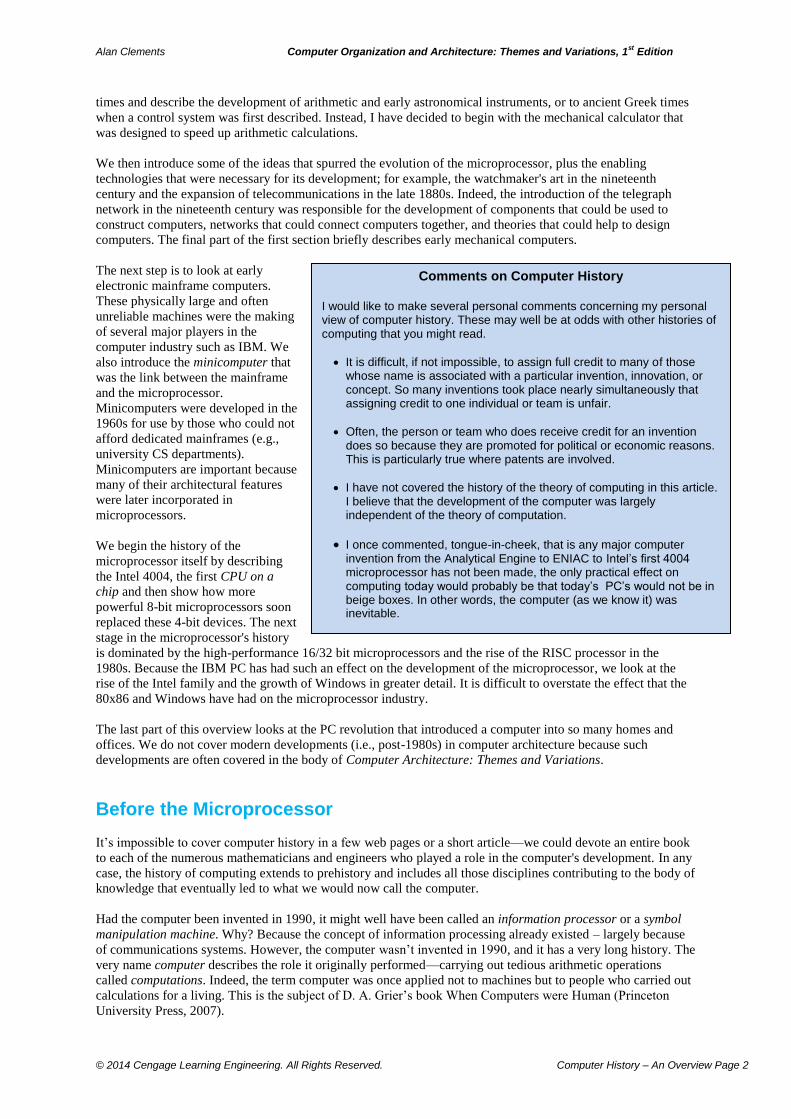
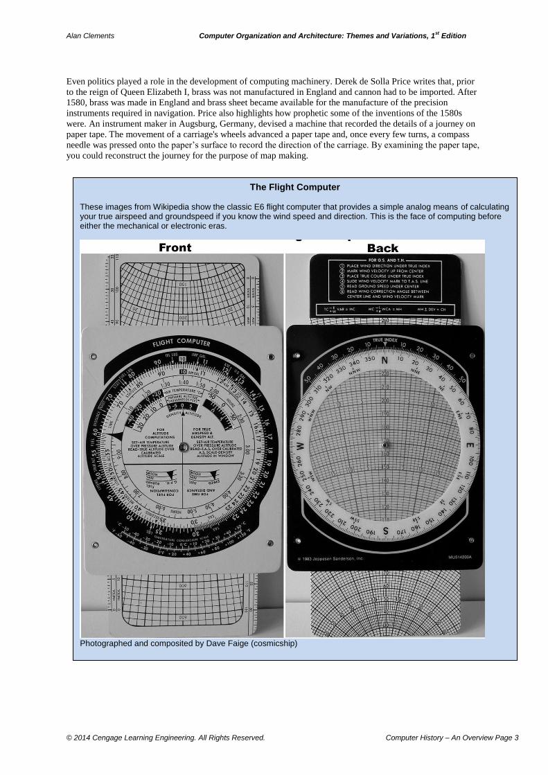
The Flight Computer These images from Wikipedia show the classic E6 flight computer that provides a simple analog means of calculating your true airspeed and groundspeed if you know the wind speed and direction. This is the face of computing before either the mechanical or electronic eras.
Photographed and composited by Dave Faige (cosmicship)
Even politics played a role in the development of computing machinery. Derek de Solla Price writes that, prior
to the reign of Queen Elizabeth I, brass was not manufactured in England and cannon had to be imported. After
1580, brass was made in England and brass sheet became available for the manufacture of the precision
instruments required in navigation. Price also highlights how prophetic some of the inventions of the 1580s
were. An instrument maker in Augsburg, Germany, devised a machine that recorded the details of a journey on
paper tape. The movement of a carriage's wheels advanced a paper tape and, once every few turns, a compass
needle was pressed onto the paper’s surface to record the direction of the carriage. By examining the paper tape,
you could reconstruct the journey for the purpose of map making.
Alan Clements Computer Organization and Architecture: Themes and Variations, 1st Edition
© 2014 Cengage Learning Engineering. All Rights Reserved. Computer History – An Overview Page 4
By the middle of the seventeenth century, several mechanical aids to calculation had been devised. These were
largely analog devices in contrast to the digital calculators we discuss shortly. Analog calculators used moving
rods, bars, or disks to perform calculations. One engraved scale was moved against another and then the result
of the calculation was read. The precision of these calculators depended on how fine the engravings on the scale
were made and how well the scale was read. Up to the 1960s, engineers used a modern version of these analog
devices called a slide rule. Even today, some aircraft pilots (largely those flying for fun in light aircraft) use a
mechanical contraption with a rotating disk and a sliding scale to calculate their true airspeed and heading from
their indicated airspeed, track, wind speed and direction (see the panel). However, since the advent of the pocket
calculator many pilots now use electronic devices to perform flight-related calculations.
Mathematics and Navigation
Mathematics was invented for two reasons. The most obvious reason was to blight the lives of generations of
high school students by forcing them to study geometry, trigonometry, and algebra. A lesser reason is that
mathematics is a powerful tool enabling us to describe the world, and, more importantly, to make predictions
about it. Long before the ancient Greek civilization flowered, humans had devised numbers, the abacus (a
primitive calculating device), and algebra. The very word digital is derived from the Latin word digitus (finger)
and calculate is derived from the Latin word calculus (pebble).
Activities from farming to building require calculations. The mathematics of measurement and geometry were
developed to enable the construction of larger and more complex buildings. Extending the same mathematics
allowed people to travel reliably from place to place without getting lost. Mathematics allowed people to predict
eclipses and to measure time.
As society progressed, trading routes grew and people traveled further and further. Longer journeys required
more reliable navigation techniques and provided an incentive to improve measurement technology. The great
advantage of a round Earth is that you don’t fall off the edge after a long sea voyage. On the other hand, a round
Earth forces you to develop spherical trigonometry to deal with navigation over distances greater than a few
miles. You also have to develop the sciences of astronomy and optics to determine your location by observing
the position of the sun, moon, stars, and planets. Incidentally, the ancient Greeks measured the diameter of the
Earth and, by 150 AD; the Greek cartographer Ptolemy had produced a world atlas that placed the prime
meridian through the Fortunate Islands (now called the Canaries, located off the west coast of Africa).
The development of navigation in the eighteenth century was probably one of the most important driving forces
towards automated computation. It’s easy to tell how far north or south of the equator you are—you simply
measure the height of the sun above the horizon at midday and then use the sun’s measured elevation (together
with the date) to work out your latitude. Unfortunately, calculating your longitude relative to the prime meridian
through Greenwich in England is very much more difficult. Longitude is determined by comparing your local
time (obtained by observing the angle of the sun) with the time at Greenwich; for example, if you find that the
local time is 8 am and your chronometer tells you that it’s 11 am in Greenwich, you must be three hours west of
Greenwich. Since the Earth rotates once is 24 hours, 3 hours is 3/24 or 1/8 of a revolution; that is, you are
360°/8 = 45° west of Greenwich.
The rush to develop a chronometer in the eighteenth century, that could keep time to an accuracy of a few
seconds during a long voyage, was as exciting as the space-race was to those of the 1960s. The technology used
to construct accurate chronometers was later used to make the first mechanical computers. Dava Sobel tells the
story of the quest to determine longitude in her book Longitude.
The mathematics of navigation uses trigonometry, which is concerned with the relationship between the sides
and the angles of a triangle. In turn, trigonometry requires an accurate knowledge of the sine, cosine, and
tangent of an angle. Not very long ago (prior to the 1970s), high school students obtained the sine of an angle in
exactly the same way as they did hundreds of years ago—by looking it up in a book containing a large table of
sines. In the 1980s, students simply punched the angle into a pocket calculator and hit the appropriate button to
calculate the appropriate since, cosine, square root, or any other common function. Today, the same students
have an application on their cell phones or iPads that does the same thing.
Those who originally devised tables of sines and other mathematical functions (e.g., square roots and
logarithms) had to do a lot of calculation by hand. If x is in radians (where 2 radians = 360) and x < 1, the
expression for sin(x) can be written as an infinite series of the form
Alan Clements Computer Organization and Architecture: Themes and Variations, 1st Edition
© 2014 Cengage Learning Engineering. All Rights Reserved. Computer History – An Overview Page 5
)!12()1(....
!7!5!3)sin(
12753
n
xxxxxx
nn
In order to calculate a sine, you convers the angle in degrees to radians and then apply the above formula.
Although the calculation of sin(x) requires the summation of an infinite number of terms, you can obtain an
approximation to sin(x) by adding just a handful of terms together, because xn tends towards zero as n increases
for x << 1.
Let’s test this formula. Suppose we wish to calculate the value of sin 15. This angle corresponds to 15/2
radians = 0.2617993877991.
Step 1: sin(x) = x = 0.2617993878
Step 2: sin(x) = x – x3/3! = 0.2588088133
Step 3: sin(x) = x – x3/3! + x
5/5! = 0.2588190618
The actual value of sin 15 is 0.2588190451, which differs from the calculated value only at the eighth decimal
position.
When the tables of values for sin(x) were compiled many years ago, armies of clerks had to do all the arithmetic
the hard way—by means of pencil and paper. As you can imagine, people looked for a better method of
compiling these tables.
An important feature of the formula for sin(x) is that it involves nothing more than the repetition of fundamental
arithmetic operations (addition, subtraction, multiplication, and division). The first term in the series is x itself.
The second term is -x3/3!, which is derived from the first term by multiplying it by x
2 and dividing it by 1 × 2 ×
3. The third term is +x5/5!, which is obtained by multiplying the second term by x
2 and dividing it by 4 × 5, and
so on. As you can see, each new term is formed by multiplying the previous term by –x2 and dividing it by
2n(2n + 1), where n is number of the term. The fundamentally easy and repetitive nature of such calculation was
not lost on people and they began to look for ways of automating alculation.
The Era of Mechanical Computers
Let’s return to the history of the computer. Although the electronic computer belongs to this century,
mechanical computing devices have existed for a very long time. The abacus was in use in the Middle East and
Asia several thousand years ago. In about 1590, the Scottish Nobleman John Napier invented logarithms and an
aid to multiplication called Napier’s Bones. These so-called bones consisted of a set of rectangular rods, each
marked with a number at the top and its multiples down its length; for example, the rod marked “6” had the
numbers 0, 12, 18, 24, etc., engraved along its length. By aligning rods (e.g., rods 2, 7, and 5) you could
multiply 275 by another number by adding the digits in the appropriate row. This reduced the complex task of
multiplication to the rather easier task of addition.
A few years later, William Oughtred invented the slide rule, a means of multiplying numbers that used scales
engraved on two wooden (and later plastic) rules that were moved against each other. The number scales were
logarithmic and converted multiplication into addition because adding the logarithms of two numbers performs
their multiplication. The slide rule became the standard means of carrying out engineering calculations and was
in common use until the 1960s. After the mid-1970s, the introduction of the electronic calculator killed off slide
rules. We’ve already mentioned that some pilots still use mechanical analog computers to calculate ground
speed from airspeed or the angle of drift due to a cross wind.
During the seventeenth century, major advances were made in watch-making; for example, in 1656 Christiaan
Huygens designed the first pendulum-controlled clock. The art of watch-making helped develop the gear wheels
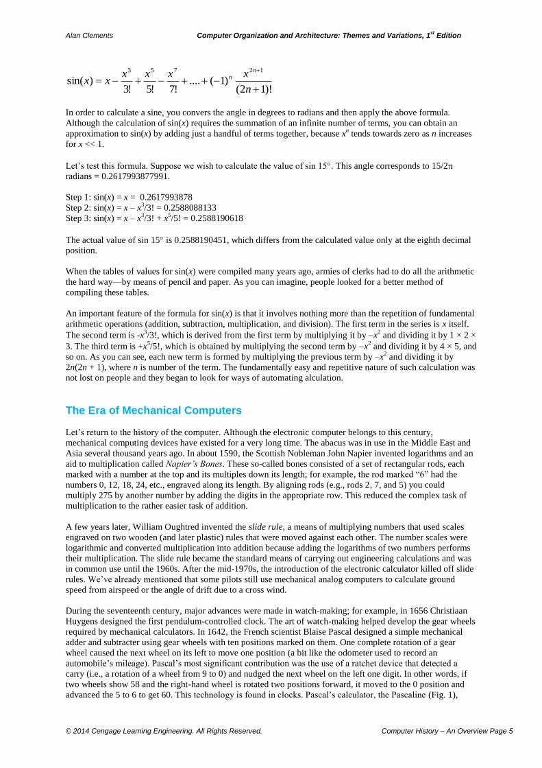
required by mechanical calculators. In 1642, the French scientist Blaise Pascal designed a simple mechanical
adder and subtracter using gear wheels with ten positions marked on them. One complete rotation of a gear
wheel caused the next wheel on its left to move one position (a bit like the odometer used to record an
automobile’s mileage). Pascal’s most significant contribution was the use of a ratchet device that detected a
carry (i.e., a rotation of a wheel from 9 to 0) and nudged the next wheel on the left one digit. In other words, if
two wheels show 58 and the right-hand wheel is rotated two positions forward, it moved to the 0 position and
advanced the 5 to 6 to get 60. This technology is found in clocks. Pascal’s calculator, the Pascaline (Fig. 1),
Alan Clements Computer Organization and Architecture: Themes and Variations, 1st Edition
© 2014 Cengage Learning Engineering. All Rights Reserved. Computer History – An Overview Page 6
could perform addition only. Subtraction was possible by the adding of complements; for example, the tens
complement of 2748 is 9999 – 2748 + 1 = 7251 + 1 = 7252. If we add this to another number, it is the same as
subtraction 2748. Consider 6551. If we add 6551 + 7252 we get 1803. If we subtract 6551 – 2748 we get 803.
These two answers are the same apart from the leading 1 in the complementary addition which is ignored. This a
technique that was later adopted by digital computers to perform binary subtraction by the addition of
compliments.
In fact, Wilhelm Schickard, rather than Pascal, is now generally credited with the invention of the first
mechanical calculator. His device, created in 1623, was more advanced than Pascal's because it could also
perform partial multiplication. Schickard died in a plague and his invention didn’t receive the recognition it
merited. Such near simultaneous developments have been a significant feature of the history of computer
hardware.
The German mathematician Gottfried Wilhelm Leibnitz was familiar with Pascal’s work and built a mechanical
calculator in 1694 that could perform addition, subtraction, multiplication, and division. Later versions of
Leibnitz's calculator were used until electronic computers became available in the 1940s.
Within a few decades, mechanical computing devices advanced to the stage where they could perform addition,
subtraction, multiplication, and division—all the operations required by armies of clerks to calculate the
trigonometric functions we mentioned earlier.
Fig. 1 Pascal’s calculator: the Pascaline (David Monniaux)
The Industrial Revolution and Early Control Mechanisms
If navigation generated a desire for mechanized computing, other developments provided important steps along
the path to the computer. By about 1800, the Industrial Revolution in Europe was well under way. Weaving was
one of the first industrial processes to be mechanized. A weaving loom passes a shuttle pulling a horizontal
thread to and fro between vertical threads held in a frame. By changing the color of the thread pulled by the
shuttle and selecting whether the shuttle passes in front of or behind the vertical threads, you can weave a
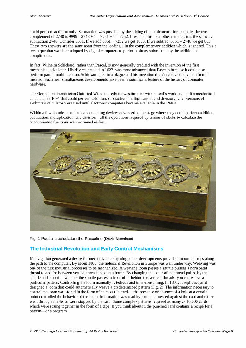
particular pattern. Controlling the loom manually is tedious and time-consuming. In 1801, Joseph Jacquard
designed a loom that could automatically weave a predetermined pattern (Fig. 2). The information necessary to
control the loom was stored in the form of holes cut in cards—the presence or absence of a hole at a certain
point controlled the behavior of the loom. Information was read by rods that pressed against the card and either
went through a hole, or were stopped by the card. Some complex patterns required as many as 10,000 cards,
which were strung together in the form of a tape. If you think about it, the punched card contains a recipe for a
pattern—or a program.
Alan Clements Computer Organization and Architecture: Themes and Variations, 1st Edition
© 2014 Cengage Learning Engineering. All Rights Reserved. Computer History – An Overview Page 7
The notion of a program appears elsewhere in the mechanical world. Consider the music box that plays a tune
when you open it. A clockwork mechanism rotates a drum whose surface is embedded with spikes or pins. A
row of thin metal strips, the teeth of a steel comb, are located along the side of the drum, but don’t quite touch
the drum’s surface. As the drum rotates, a pin sticking out of the drum meets one of the strips and drags the strip
along with it. Eventually, the pin rotates past the strip’s end and the strip falls back with a twang. By tuning each
strip to a suitable musical note, a tune can be played as the drum rotates. The location of the pegs on the surface
of the drum determines the sequence of notes played.
The computer historian Brian Randell points out that this pegged drum mechanical programmer has a long
history. Heron of Alexandria described a pegged drum control mechanism about 100 AD. A rope is wound
round a drum and then hooked around a peg on the drum's surface. Then the rope is wound in the opposite
direction. This process can be repeated as many times as you like, with one peg for each reversal of direction. If
you pull the rope, the drum will rotate. However, when a peg is encountered, the direction of rotation will
change. The way in which the string is wound round the drum (i.e., its helical pitch) determines the drum’s
speed of rotation. This mechanism allows you to predefine a sequence of operations; for example,
clockwise/slow/long; counterclockwise/slow/short. Such technology could be used to control temple doors.
Although Heron's mechanism may seem a long way from the computer, it demonstrates that the intellectual
notions of control and sequencing have existed for a very long time.
Fig. 2 The Jacquard loom (Edal Anton Lefterov)
Babbage and the Computer
Two significant advances in computing were made by Charles Babbage, a British mathematician born in 1792,
his difference engine and his analytical engine. Like other mathematicians, Babbage had to perform all
calculations by hand, and sometimes he had to laboriously correct errors in published mathematical tables.
Living in the age of steam, it was quite natural for Babbage to ask himself whether mechanical means could be
applied to arithmetic calculations. Babbage’s difference engine took mechanical calculation one step further by
performing a sequence of additions and multiplications in order to calculate the coefficients of a polynomial
using the method of finite differences.
Babbage wrote papers about concept of mechanical calculators and applied to the British Government for
funding to implement them, and received what was probably the world’s first government grant for computer
Alan Clements Computer Organization and Architecture: Themes and Variations, 1st Edition
© 2014 Cengage Learning Engineering. All Rights Reserved. Computer History – An Overview Page 8
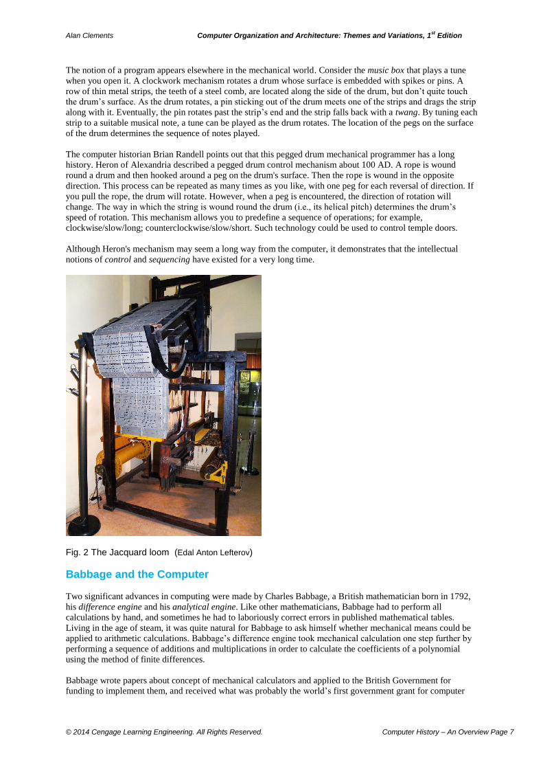
research. Unfortunately, Babbage didn’t actually build his difference engine calculating machine. However, he
and his engineer, Clement, constructed a part of the working model of the calculator between 1828 and 1833
(Fig. 3).
Babbage’s difference engine project was cancelled in 1842 because of increasing costs. He did design a simpler
difference engine using 31-digit numbers to handle 7th-order differences, but no one was interested in financing
it. However, in 1853, George Scheutz in Sweden constructed a working difference engine using 15-digit
arithmetic and 4th-order differences. Like Babbage, Scheutz’s work was government financed. Incidentally, in
1991, a team at the Science Museum in London used modern construction techniques to build Babbage’s
difference engine. It worked.
The difference engine mechanized the calculation of polynomial functions and automatically printed the result.
The difference engine was a complex array of interconnected gears and linkages that performed addition and
subtraction rather like Pascal’s mechanical adder. However, it was a calculator rather than a computer because
it could carry out only a set of predetermined operations.
Fig. 3 A portion of Babbage’s difference engine (Geni)
Babbage’s difference engine employed a technique called finite differences to calculate polynomial functions.
Remember that trigonometric functions can be expressed as polynomials in the form a0x + a1x1 + a2x
2 + … The
difference engine can evaluate such expressions automatically.
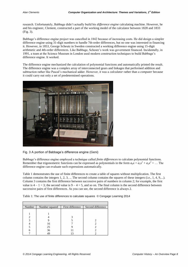
Table 1 demonstrates the use of finite differences to create a table of squares without multiplication. The first
column contains the integers 1, 2, 3, ... The second column contains the squares of these integers (i.e., 1, 4, 9,...).
Column 3 contains the first difference between successive pairs of numbers in column 2; for example, the first
value is 4 1 = 3; the second value is 9 4 = 5, and so on. The final column is the second difference between
successive pairs of first differences. As you can see, the second difference is always 2.
Table 1: The use of finite differences to calculate squares © Cengage Learning 2014
Number Number squared First difference Second difference
1 1
2 4 3
3 9 5 2
4 16 7 2
5 25 9 2
6 36 11 2
7 49 13 2
Alan Clements Computer Organization and Architecture: Themes and Variations, 1st Edition
© 2014 Cengage Learning Engineering. All Rights Reserved. Computer History – An Overview Page 9
Suppose we want to calculate the value of 82 using finite differences. We simply use this table in reverse by
starting with the second difference and working back to the result. If the second difference is 2, the next first
difference (after 72) is 13 + 2 = 15. Therefore, the value of 8
2 is the value of 7
2 plus the first difference; that is 49
+ 15 = 64. We have generated 82 without using multiplication. This technique can be extended to evaluate many
other mathematical functions.
Charles Babbage went on to design the analytical engine that was to be capable of performing any mathematical
operation automatically. This truly remarkable and entirely mechanical device was nothing less than a general-
purpose computer that could be programmed. The analytical engine included many of the elements associated
with a modern electronic computer—an arithmetic processing unit that carries out all the calculations, a memory
that stores data, and input and output devices. Unfortunately, the sheer scale of the analytical engine rendered its
construction, at that time, impossible. However, it is not unreasonable to call Babbage the father of the computer
because his machine incorporated many of the intellectual concepts at the heart of the computer.
Babbage envisaged that his analytical engine would be controlled by punched cards similar to those used to
control the operation of the Jacquard loom. Two types of punched card were required. Operation cards specified
the sequence of operations to be carried out by the analytical engine and variable cards specified the locations in
store of inputs and outputs.
One of Babbage's contributions to computing was the realization that it is better to construct one arithmetic unit
and share it between other parts of the difference engine than to construct multiple arithmetic units. The part of
the analytical engine that performed the calculations was the mill (now called the arithmetic logic unit [ALU])
and the part that held information was called the store. In the 1970s, mainframe computers made by ICL
recorded computer time in mills in honor of Babbage.
A key, if not the key, element of the computer is its ability to make a decision based on the outcome of a
previous operation; for example, the action IF x > 4, THEN y = 3 represents such a conditional action because
the value 3 is assigned to y only if x is greater than 4. Babbage described the conditional operation that was to
be implemented by testing the sign of a number and then performing one of two operations depending on the
sign.
Because Babbage’s analytical engine used separate stores (i.e., punched cards) for data and instructions, it
lacked one of the principal features of modern computers—the ability of a program to operate on its own code.
However, Babbage’s analytical engine incorporated more computer-like features than some of the machines in
the 1940s that are credited as the first computers.
One of Babbage’s collaborators was Ada Gordon, a mathematician who became interested in the analytical
engine when she translated a paper on it from French to English. When Babbage discovered the paper he asked
her to expand it. She added about 40 pages of notes about the machine and provided examples of how the
proposed Analytical Engine could be used to solve mathematical problems.
Ada worked closely with Babbage, and it’s been reported that
she even suggested the use of the binary system rather than
the decimal system to store data. She noticed that certain
groups of operations are carried out over and over again
during the course of a calculation and proposed that a
conditional instruction be used to force the analytical engine
to perform the same sequence of operations many times. This
action is the same as the repeat or loop function found in
most of today’s high-level languages.
Ada devised algorithms to perform the calculation of Bernoulli numbers, which makes her one of the founders
of numerical computation that combines mathematics and computing. Some regard Ada as the world’s first
computer programmer. She constructed an algorithm a century before programming became a recognized
discipline and long before any real computers were constructed. In the 1970s, the US Department of Defense
commissioned a language for real-time computing and named it Ada in her honor.
Mechanical computing devices continued to be used in compiling mathematical tables and performing the
arithmetic operations used by everyone from engineers to accountants until about the 1960s. The practical high-
speed computer had to await the development of the electronics industry.
Ada’s Name There is some confusion surrounding Ada's family name in articles about her. Ada was born Gordon and married William King. King was later made the Earl of Lovelace and Ada became the Countess of Lovelace. Her father was the Lord Byron. Consequently, her name is either Ada Gordon or Ada King, but never Ada Lovelace or Ada Byron.
Alan Clements Computer Organization and Architecture: Themes and Variations, 1st Edition
© 2014 Cengage Learning Engineering. All Rights Reserved. Computer History – An Overview Page 10
Before we introduce the first electromechanical computers, we describe a very important step in the history of
the computer, the growth of the technology that made electrical and electronic computers possible.
Enabling Technology—The Telegraph
In my view, one of the most important stages in the development of the computer was the invention of the
telegraph. In the early nineteenth century, King Maximilian had seen how the French visual semaphore system
had helped Napoleon's military campaigns, and in 1809 he asked the Bavarian Academy of Sciences to devise a
scheme for high-speed communication over long distances. Sömmering designed a crude telegraph that used 35
conductors, one for each character. Sömmering's telegraph transmited electricity from a battery down one of the
35 wires where, at the receiver, the current was passed through a tube of acidified water. Passing a current
resulted in the dissociation of water into oxygen and hydrogen. The bubbles that thus appeared in one of the 35
glass tubes were detected and the corresponding character was noted down. Sömmering's telegraph was
ingenious, but too slow to be practical.
In 1819, H. C. Oersted made one of the greatest discoveries of all time when he found that an electric current
creates a magnetic field round a conductor. Passing a current through a coil made it possible to create a
magnetic field at will. Since the power source and on/off switch (or key) could be miles away from the compass
needle, invention became the telegraph.
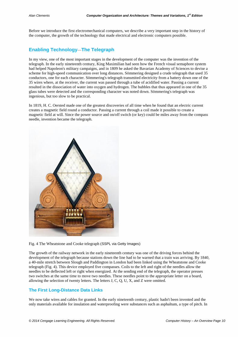
Fig. 4 The Wheatstone and Cooke telegraph (SSPL via Getty Images)
The growth of the railway network in the early nineteenth century was one of the driving forces behind the
development of the telegraph because stations down the line had to be warned that a train was arriving. By 1840,
a 40-mile stretch between Slough and Paddington in London had been linked using the Wheatstone and Cooke
telegraph (Fig. 4). This device employed five compasses. Coils to the left and right of the needles allow the
needles to be deflected left or right when energized. At the sending end of the telegraph, the operator presses
two switches at the same time to move two needles. These needles point to the appropriate letter on a board,
allowing the selection of twenty letters. The letters J, C, Q, U, X, and Z were omitted.
The First Long-Distance Data Links
We now take wires and cables for granted. In the early nineteenth century, plastic hadn't been invented and the
only materials available for insulation and waterproofing were substances such as asphaltum, a type of pitch. In
Alan Clements Computer Organization and Architecture: Themes and Variations, 1st Edition
© 2014 Cengage Learning Engineering. All Rights Reserved. Computer History – An Overview Page 11
1843, a form of rubber called gutta percha was discovered and used to insulate the signal-carrying path in
cables. The Atlantic Telegraph Company created an insulated cable for underwater use. It comprised a single
copper conductor made of seven twisted strands, surrounded by gutta percha insulation and protected by a ring
of 18 iron wires coated with hemp and tar.
Submarine cable telegraphy began with a cable crossing the English Channel to France in 1850. The cable failed
after only a few messages had been exchanged, but a more successful attempt was made the following year.
Transatlantic cable laying from Ireland began in 1857, but was abandoned when the strain of the cable
descending to the ocean bottom caused it to snap under its own weight. The Atlantic Telegraph Company tried
again in 1858. Again, the cable broke after only three miles, but the two cable-laying ships managed to splice
the two ends. The cable eventually reached Newfoundland in August 1858 after suffering several more breaks
and storm damage.
It soon became clear that this cable wasn't going to be a commercial success. The receiver used the magnetic
field from current in the cable to deflect a magnetized needle. The voltage at the transmitting end used to drive a
current down the cable was approximately 600 V. However, after crossing the Atlantic the signal was too weak
to be reliably detected, so they raised the voltage to about 2,000 V to drive more current along the cable and
improve the detection process. Unfortunately, such a high voltage burned through the primitive insulation,
shorted the cable, and destroyed the first transatlantic telegraph link after about 700 messages had been
transmitted in three months.
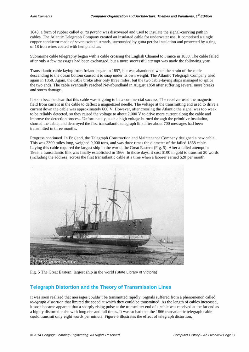
Progress continued. In England, the Telegraph Construction and Maintenance Company designed a new cable.
This was 2300 miles long, weighed 9,000 tons, and was three times the diameter of the failed 1858 cable.
Laying this cable required the largest ship in the world, the Great Eastern (Fig. 5). After a failed attempt in
1865, a transatlantic link was finally established in 1866. In those days, it cost $100 in gold to transmit 20 words
(including the address) across the first transatlantic cable at a time when a laborer earned $20 per month.
Fig. 5 The Great Eastern: largest ship in the world (State Library of Victoria)
Telegraph Distortion and the Theory of Transmission Lines
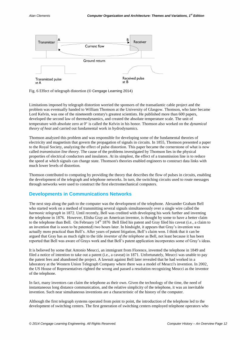
It was soon realized that messages couldn’t be transmitted rapidly. Signals suffered from a phenomenon called
telegraph distortion that limited the speed at which they could be transmitted. As the length of cables increased,
it soon became apparent that a sharply rising pulse at the transmitter end of a cable was received at the far end as
a highly distorted pulse with long rise and fall times. It was so bad that the 1866 transatlantic telegraph cable
could transmit only eight words per minute. Figure 6 illustrates the effect of telegraph distortion.
Alan Clements Computer Organization and Architecture: Themes and Variations, 1st Edition
© 2014 Cengage Learning Engineering. All Rights Reserved. Computer History – An Overview Page 12
Fig. 6 Effect of telegraph distortion (© Cengage Learning 2014)
Limitations imposed by telegraph distortion worried the sponsors of the transatlantic cable project and the
problem was eventually handed to William Thomson at the University of Glasgow. Thomson, who later became
Lord Kelvin, was one of the nineteenth century's greatest scientists. He published more than 600 papers,
developed the second law of thermodynamics, and created the absolute temperature scale. The unit of
temperature with absolute zero at 0 is called the Kelvin in his honor. Thomson also worked on the dynamical
theory of heat and carried out fundamental work in hydrodynamics.
Thomson analyzed this problem and was responsible for developing some of the fundamental theories of
electricity and magnetism that govern the propagation of signals in circuits. In 1855, Thomson presented a paper
to the Royal Society, analyzing the effect of pulse distortion. This paper became the cornerstone of what is now
called transmission line theory. The cause of the problems investigated by Thomson lies in the physical
properties of electrical conductors and insulators. At its simplest, the effect of a transmission line is to reduce
the speed at which signals can change state. Thomson's theories enabled engineers to construct data links with
much lower levels of distortion.
Thomson contributed to computing by providing the theory that describes the flow of pulses in circuits, enabling
the development of the telegraph and telephone networks. In turn, the switching circuits used to route messages
through networks were used to construct the first electromechanical computers.
Developments in Communications Networks
The next step along the path to the computer was the development of the telephone. Alexander Graham Bell
who started work on a method of transmitting several signals simultaneously over a single wire called the
harmonic telegraph in 1872. Until recently, Bell was credited with developing his work further and inventing
the telephone in 1876. However, Elisha Gray an American inventor, is thought by some to have a better claim
to the telephone than Bell. On February 14th
1876 Bell filed his patent and Gray filed his caveat (i.e., a claim to
an invention that is soon to be patented) two hours later. In hindsight, it appears that Gray’s invention was
actually more practical than Bell’s. After years of patent litigation, Bell’s claim won. I think that it can be
argued that Gray has as much right to the title inventor of the telephone as Bell, not least because it has been
reported that Bell was aware of Grays work and that Bell’s patent application incorporates some of Gray’s ideas.
It is believed by some that Antonio Meucci, an immigrant from Florence, invented the telephone in 1849 and
filed a notice of intention to take out a patent (i.e., a caveat) in 1871. Unfortunately, Meucci was unable to pay
the patent fees and abandoned the project. A lawsuit against Bell later revealed that he had worked in a
laboratory at the Western Union Telegraph Company where there was a model of Meucci's invention. In 2002,
the US House of Representatives righted the wrong and passed a resolution recognizing Meucci as the inventor
of the telephone.
In fact, many inventors can claim the telephone as their own. Given the technology of the time, the need of
instantaneous long distance communication, and the relative simplicity of the telephone, it was an inevitable
invention. Such near simultaneous inventions are a characteristic of the history of the computer.
Although the first telegraph systems operated from point to point, the introduction of the telephone led to the
development of switching centers. The first generation of switching centers employed telephone operators who
Alan Clements Computer Organization and Architecture: Themes and Variations, 1st Edition
© 2014 Cengage Learning Engineering. All Rights Reserved. Computer History – An Overview Page 13
manually plugged a subscriber's line into a line connected to the next switching center in the link. By the end of
the nineteenth century, the infrastructure of computer networks was already in place.
The inventions of the telegraph and telephone gave us signals that we could create at one place and receive at
another, and telegraph wires and undersea cables gave us point-to-point connectivity. The one thing missing was
point-to-point switching.
At the end of the nineteenth century, telephone lines were switched from center to center by human operators in
manual telephone exchanges. In 1897, an undertaker called Strowger was annoyed to find that he was not
getting the trade he expected. Strowger believed that the local telephone operator was connecting prospective
clients to his competitor. So, he cut out the human factor by inventing the automatic telephone exchange that
used electromechanical devices to route calls between exchanges. This invention required the rotary dial that has
all but disappeared today.
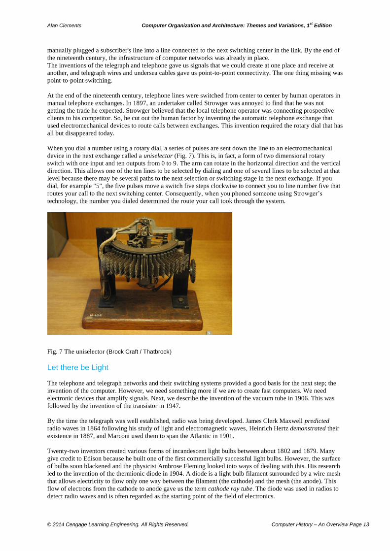
When you dial a number using a rotary dial, a series of pulses are sent down the line to an electromechanical
device in the next exchange called a uniselector (Fig. 7). This is, in fact, a form of two dimensional rotary
switch with one input and ten outputs from 0 to 9. The arm can rotate in the horizontal direction and the vertical
direction. This allows one of the ten lines to be selected by dialing and one of several lines to be selected at that
level because there may be several paths to the next selection or switching stage in the next exchange. If you
dial, for example "5", the five pulses move a switch five steps clockwise to connect you to line number five that
routes your call to the next switching center. Consequently, when you phoned someone using Strowger’s
technology, the number you dialed determined the route your call took through the system.
Fig. 7 The uniselector (Brock Craft / Thatbrock)
Let there be Light
The telephone and telegraph networks and their switching systems provided a good basis for the next step; the
invention of the computer. However, we need something more if we are to create fast computers. We need
electronic devices that amplify signals. Next, we describe the invention of the vacuum tube in 1906. This was
followed by the invention of the transistor in 1947.
By the time the telegraph was well established, radio was being developed. James Clerk Maxwell predicted
radio waves in 1864 following his study of light and electromagnetic waves, Heinrich Hertz demonstrated their
existence in 1887, and Marconi used them to span the Atlantic in 1901.
Twenty-two inventors created various forms of incandescent light bulbs between about 1802 and 1879. Many
give credit to Edison because he built one of the first commercially successful light bulbs. However, the surface
of bulbs soon blackened and the physicist Ambrose Fleming looked into ways of dealing with this. His research
led to the invention of the thermionic diode in 1904. A diode is a light bulb filament surrounded by a wire mesh
that allows electricity to flow only one way between the filament (the cathode) and the mesh (the anode). This
flow of electrons from the cathode to anode gave us the term cathode ray tube. The diode was used in radios to
detect radio waves and is often regarded as the starting point of the field of electronics.
Alan Clements Computer Organization and Architecture: Themes and Variations, 1st Edition
© 2014 Cengage Learning Engineering. All Rights Reserved. Computer History – An Overview Page 14
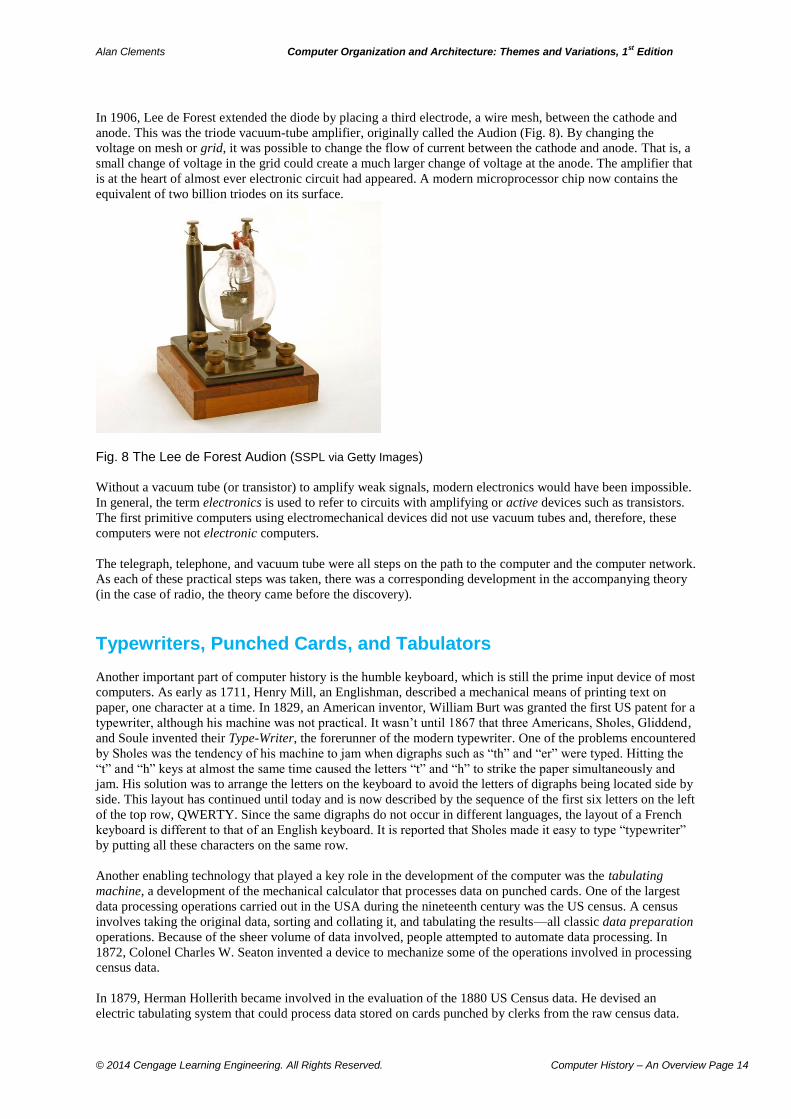
In 1906, Lee de Forest extended the diode by placing a third electrode, a wire mesh, between the cathode and
anode. This was the triode vacuum-tube amplifier, originally called the Audion (Fig. 8). By changing the
voltage on mesh or grid, it was possible to change the flow of current between the cathode and anode. That is, a
small change of voltage in the grid could create a much larger change of voltage at the anode. The amplifier that
is at the heart of almost ever electronic circuit had appeared. A modern microprocessor chip now contains the
equivalent of two billion triodes on its surface.
Fig. 8 The Lee de Forest Audion (SSPL via Getty Images)
Without a vacuum tube (or transistor) to amplify weak signals, modern electronics would have been impossible.
In general, the term electronics is used to refer to circuits with amplifying or active devices such as transistors.
The first primitive computers using electromechanical devices did not use vacuum tubes and, therefore, these
computers were not electronic computers.
The telegraph, telephone, and vacuum tube were all steps on the path to the computer and the computer network.
As each of these practical steps was taken, there was a corresponding development in the accompanying theory
(in the case of radio, the theory came before the discovery).
Typewriters, Punched Cards, and Tabulators
Another important part of computer history is the humble keyboard, which is still the prime input device of most
computers. As early as 1711, Henry Mill, an Englishman, described a mechanical means of printing text on
paper, one character at a time. In 1829, an American inventor, William Burt was granted the first US patent for a
typewriter, although his machine was not practical. It wasn’t until 1867 that three Americans, Sholes, Gliddend,
and Soule invented their Type-Writer, the forerunner of the modern typewriter. One of the problems encountered
by Sholes was the tendency of his machine to jam when digraphs such as “th” and “er” were typed. Hitting the
“t” and “h” keys at almost the same time caused the letters “t” and “h” to strike the paper simultaneously and
jam. His solution was to arrange the letters on the keyboard to avoid the letters of digraphs being located side by
side. This layout has continued until today and is now described by the sequence of the first six letters on the left
of the top row, QWERTY. Since the same digraphs do not occur in different languages, the layout of a French
keyboard is different to that of an English keyboard. It is reported that Sholes made it easy to type “typewriter”
by putting all these characters on the same row.
Another enabling technology that played a key role in the development of the computer was the tabulating
machine, a development of the mechanical calculator that processes data on punched cards. One of the largest
data processing operations carried out in the USA during the nineteenth century was the US census. A census
involves taking the original data, sorting and collating it, and tabulating the results—all classic data preparation
operations. Because of the sheer volume of data involved, people attempted to automate data processing. In
1872, Colonel Charles W. Seaton invented a device to mechanize some of the operations involved in processing
census data.
In 1879, Herman Hollerith became involved in the evaluation of the 1880 US Census data. He devised an
electric tabulating system that could process data stored on cards punched by clerks from the raw census data.
Alan Clements Computer Organization and Architecture: Themes and Variations, 1st Edition
© 2014 Cengage Learning Engineering. All Rights Reserved. Computer History – An Overview Page 15
Hollerith's electric tabulating machine could read cards, tabulate the information on the cards (i.e., count and
record), and then sort the cards. These tabulators employed a new form of electromechanical counting
mechanism. Moreover, punched cards reduced human reading errors and provided an effectively unlimited
storage capacity. By copying cards, processing could even be carried out in parallel. During the 1890s and
1900s, Hollerith made a whole series of inventions and improvements, all geared towards automatic data
collection, processing, and printing.
The Hollerith Tabulating Company, eventually became one of the three that made up the Calculating-
Tabulating-Recording Corporation (CTR). This was renamed in 1924 when it became IBM.
Three threads converged to make the computer possible: Babbage’s calculating machines that perform
arithmetic (indeed, even scientific) calculations, communications technology that laid the foundations for
electronic systems and even networking, and the tabulator. The tabulator provided a means of controlling
computers, inputting/outputting data, and storing information until low-cost peripherals were to become
available after the 1970s. Moreover, the tabulator helped lay the foundations of the data processing industry.
The Analog Computer
We now take a short detour and introduce the largely forgotten analog computer that spurred the development
of its digital sibling. When people use the term computer today, they are self-evidently referring to the digital
computer. This statement was not always true, because there was an era when some computers were analog
computers. In fact, university courses on analog computing were still being taught in the 1970s.
Although popular mythology regards the computer industry as having its origins in World War II, engineers
were thinking about computing machines within a few decades of the first practical applications of electricity.
As early as 1872, the Society of Telegraph Engineers held their Fourth Ordinary General Meeting in London to
discuss electrical calculations. One strand of computing led to the development of analog computers that
simulated systems either electrically or mechanically.
Analog computers are mechanical or electronic systems that perform computations by simulating the system
they are being used to analyze or model. Probably the oldest analog computer is the hourglass. The grains of
sand in an hourglass represent time; as time passes, the sand flows from one half of the glass into the other half
through a small constriction. An hourglass is programmed by selecting the grade and quantity of the sand and
the size of the constriction. The clock is another analog computer, where the motion of the hands simulates the
passage of time. Similarly, a mercury thermometer is an analog computer that represents temperature by the
length of a column of mercury.
An electronic analog computer represents a variable (e.g., time or distance) by an electrical quantity and then
models the system being analyzed. For example, in order to analyze the trajectory of a shell fired from a field
gun, you would construct a circuit using electronic components that mimic the effect of gravity and air
resistance, etc. The analog computer might be triggered by applying a voltage step, and then the height and
distance of the shell would be given by two voltages that change with time. The output of such an analog
computer might be a trace on a CRT screen. Analog computers lack the accuracy of digital computers because
their precision is determined by the nature of the components and the ability to measure voltages and currents.
Analog computers are suited to the solution of scientific and engineering problems such as the calculation of the
stress on a beam in a bridge, rather than, for example, financial or database problems.
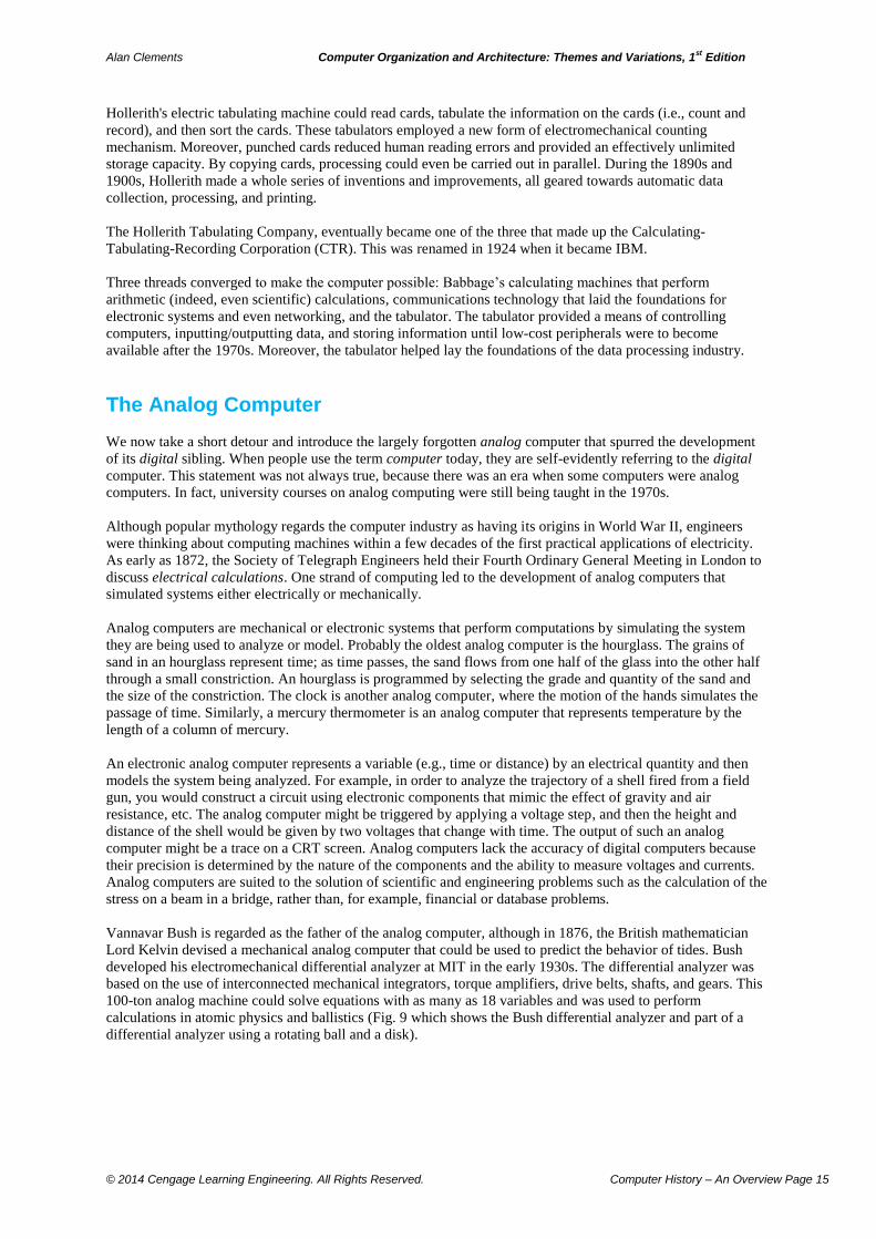
Vannavar Bush is regarded as the father of the analog computer, although in 1876, the British mathematician
Lord Kelvin devised a mechanical analog computer that could be used to predict the behavior of tides. Bush
developed his electromechanical differential analyzer at MIT in the early 1930s. The differential analyzer was
based on the use of interconnected mechanical integrators, torque amplifiers, drive belts, shafts, and gears. This
100-ton analog machine could solve equations with as many as 18 variables and was used to perform
calculations in atomic physics and ballistics (Fig. 9 which shows the Bush differential analyzer and part of a
differential analyzer using a rotating ball and a disk).
Alan Clements Computer Organization and Architecture: Themes and Variations, 1st Edition
© 2014 Cengage Learning Engineering. All Rights Reserved. Computer History – An Overview Page 16
Fig. 9 Bush's differential analyzer 1931 (public domain) Fig. 9 Harmonic analyzer disc and sphere (Andy Dingley))
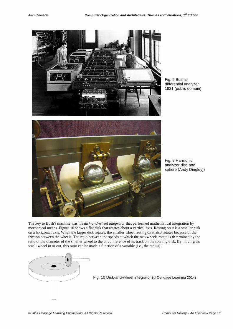
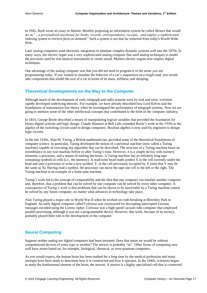
The key to Bush's machine was his disk-and-wheel integrator that performed mathematical integration by
mechanical means. Figure 10 shows a flat disk that rotates about a vertical axis. Resting on it is a smaller disk
on a horizontal axis. When the larger disk rotates, the smaller wheel resting on it also rotates because of the
friction between the wheels. The ratio between the speeds at which the two wheels rotate is determined by the
ratio of the diameter of the smaller wheel to the circumference of its track on the rotating disk. By moving the
small wheel in or out, this ratio can be made a function of a variable (i.e., the radius).
Fig. 10 Disk-and-wheel integrator (© Cengage Learning 2014)
Alan Clements Computer Organization and Architecture: Themes and Variations, 1st Edition
© 2014 Cengage Learning Engineering. All Rights Reserved. Computer History – An Overview Page 17
In 1945, Bush wrote an essay in Atlantic Monthly proposing an information system he called Memex that would
act as "…a personalized storehouse for books, records, correspondence, receipts…and employ a sophisticated
indexing system to retrieve facts on demand." Such a system is not that far removed from today's World Wide
Web.
Later analog computers used electronic integrators to simulate complex dynamic systems well into the 1970s. In
many ways, the electric organ was a very sophisticated analog computer that used analog techniques to model
the processes used by real musical instruments to create sound. Modern electric organs now employ digital
techniques.
One advantage of the analog computer was that you did not need to program it in the sense you use
programming today. If you wanted to simulate the behavior of a car’s suspension on a rough road, you would
take components that model the axis of a car in terms of its mass, stiffness, and damping.
Theoretical Developments on the Way to the Computer
Although much of the development of early telegraph and radio systems were by trial and error, scientists
rapidly developed underlying theories. For example, we have already described how Lord Kelvin laid the
foundations of transmission line theory when he investigated the performance of telegraph systems. Now we are
going to mention some of the other intellectual concepts that contributed to the birth of the computer industry.
In 1854, George Boole described a means of manipulating logical variables that provided the foundation for
binary digital systems and logic design. Claude Shannon at Bell Labs extended Boole’s work in the 1930s to the
algebra of the switching circuits used to design computers. Boolean algebra is now used by engineers to design
logic circuits.
In the late 1930s, Alan M. Turing, a British mathematician, provided some of the theoretical foundations of
computer science. In particular, Turing developed the notion of a universal machine (now called a Turing
machine) capable of executing any algorithm that can be described. The structure of a Turing machine bears no
resemblance to any real machine before or after Turing’s time. However, it is a simple device with memory
elements, a processor, and a means of making decisions. A Turing machine has an infinitely long tape
containing symbols in cells (i.e., the memory). A read/write head reads symbol X in the cell currently under the
head and uses a processor to write a new symbol, Y, in the cell previously occupied by X (note that Y may be
the same as X). Having read a symbol, the processor can move the tape one cell to the left or the right. The
Turing machine is an example of a finite state machine.
Turing’s work led to the concept of computability and the idea that one computer can emulate another computer
and, therefore, that a problem that can be solved by one computer can be solved by every other computer. A
consequence of Turing’s work is that problems that can be shown to be unsolvable by a Turing machine cannot
be solved by any future computer, no matter what advances in technology take place.
Alan Turing played a major role in World War II when he worked on code-breaking at Bletchley Park in
England. An early digital computer called Colossus was constructed for decrypting intercepted German
messages encoded using the Lorenz cipher. Colossus was a high-speed vacuum tube computer that employed
parallel processing, although it was not a programmable device. However, this work, because of its secrecy,
probably played little role in the development of the computer.
Neural Computing
Suppose neither analog nor digital computers had been invented. Does that mean we would be without
computational devices of some type or another? The answer is probably “no”. Other forms of computing may
well have arisen based on, for example, biological, chemical, or even quantum computers.
As you would expect, the human brain has been studied for a long time by the medical profession and many
attempts have been made to determine how it is constructed and how it operates. In the 1940s, scientists began
to study the fundamental element of the brain, the neuron. A neuron is a highly specialized cell that is connected
Alan Clements Computer Organization and Architecture: Themes and Variations, 1st Edition
© 2014 Cengage Learning Engineering. All Rights Reserved. Computer History – An Overview Page 18
to other neurons to form a complex network of about 1011
neurons. In 1943, a US neurophysiologist Warren
McCulloch worked with Walter Pitts to create a simple model of the neuron from analog electronic components.
Scientists have attempted to create computational devices based on networks of neurons. Such networks have
properties of both analog and digital computers. Like analog computers, they model a system and like digital
computers they can be programmed, although their programming is in terms of numerical parameters rather than
a sequence of operations. Like analog computers, they cannot be used for conventional applications such as data
processing and are more suited to tasks such as modeling the stock exchange.
The McCulloch and Pitts model of a neuron has n inputs and a single output. The ith input xi is weighted (i.e.,
multiplied) by a constant wi, so that the ith input becomes xi ∙ wi. The neuron sums all the weighted inputs to get
x0 ∙ w0. + x1 ∙ w1. +…+ xn-1 ∙ wn-1 which can be represented by xi ∙ wi. The sum of the weighted inputs is
compared with a threshold T, and the neuron fires if the sum of the weighted inputs is greater than T. A neuron
is programmed by selecting the values of the weights and T. For example, suppose that w0 = ½, w1 = ¼, x0 = 2,
x1 = 1 and T = ½. The weighted sum of the inputs is 2x ½ + 1x (– ¼) = 1 – ¼ = ¾. This is greater than T and the
neuron will fire (i.e., produce the output 1).
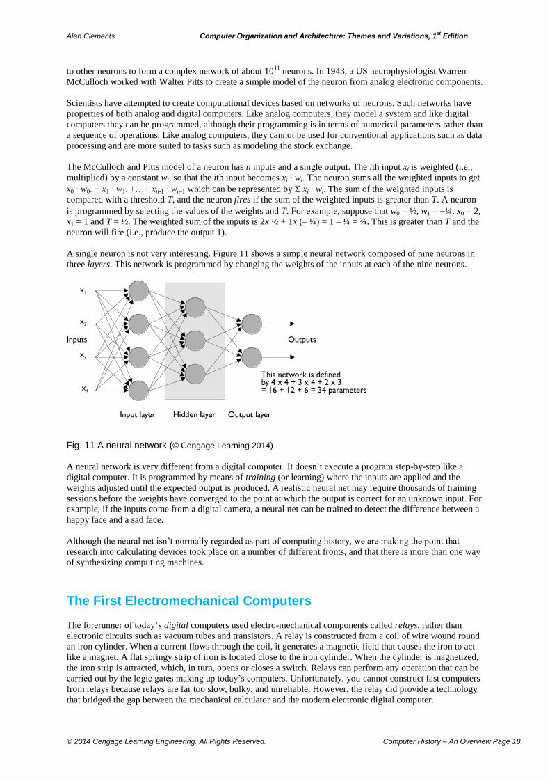
A single neuron is not very interesting. Figure 11 shows a simple neural network composed of nine neurons in
three layers. This network is programmed by changing the weights of the inputs at each of the nine neurons.
Fig. 11 A neural network (© Cengage Learning 2014)
A neural network is very different from a digital computer. It doesn’t execute a program step-by-step like a
digital computer. It is programmed by means of training (or learning) where the inputs are applied and the
weights adjusted until the expected output is produced. A realistic neural net may require thousands of training
sessions before the weights have converged to the point at which the output is correct for an unknown input. For
example, if the inputs come from a digital camera, a neural net can be trained to detect the difference between a
happy face and a sad face.
Although the neural net isn’t normally regarded as part of computing history, we are making the point that
research into calculating devices took place on a number of different fronts, and that there is more than one way
of synthesizing computing machines.
The First Electromechanical Computers The forerunner of today’s digital computers used electro-mechanical components called relays, rather than
electronic circuits such as vacuum tubes and transistors. A relay is constructed from a coil of wire wound round
an iron cylinder. When a current flows through the coil, it generates a magnetic field that causes the iron to act
like a magnet. A flat springy strip of iron is located close to the iron cylinder. When the cylinder is magnetized,
the iron strip is attracted, which, in turn, opens or closes a switch. Relays can perform any operation that can be
carried out by the logic gates making up today’s computers. Unfortunately, you cannot construct fast computers
from relays because relays are far too slow, bulky, and unreliable. However, the relay did provide a technology
that bridged the gap between the mechanical calculator and the modern electronic digital computer.
Alan Clements Computer Organization and Architecture: Themes and Variations, 1st Edition
© 2014 Cengage Learning Engineering. All Rights Reserved. Computer History – An Overview Page 19
In 1914, Torres y Quevedo, a Spanish scientist and engineer, wrote a paper describing how electromechanical
technology, such as relays, could be used to implement Babbage's analytical engine. The computer historian
Randell comments that Torres could have successfully produced Babbage’s analytical engine in the 1920s.
Torres was one of the first to appreciate that a necessary element of the computer is conditional behavior; that
is, its ability to select a future action on the basis of
a past result. Randell quotes from a paper by
Torres:
"Moreover, it is essential – being the chief objective
of Automatics – that the automata be capable of
discernment; that they can at each moment, take
account of the information they receive, or even
information they have received beforehand, in
controlling the required operation. It is necessary
that the automata imitate living beings in regulating
their actions according to their inputs, and adapt
their conduct to changing circumstances." One of the first electro-mechanical computers was
built by Konrad Zuse in Germany. Zuse’s Z2 and
Z3 computers were used in the early 1940s to
design aircraft in Germany. The heavy bombing at
the end of the Second World War destroyed Zuse’s
computers and his contribution to the development
of the computer was ignored for many years. He is
mentioned here to demonstrate that the notion of a practical computer occurred to different people in different
places. Zuse used binary arithmetic, developed floating-point-arithmetic (his Z3 computer had a 22-bit word
length, with 1 bit for the sign, 7 exponential bits and a 14-bit mantissa), and it has been claimed that his Z3
computers had all the features of a von Neumann machine apart from the stored program concept. Moreover,
because the Z3 was completed in 1941, it was the world’s first functioning programmable mechanical computer.
Zuse completed his Z4 computer in 1945. This was taken to Switzerland, where it was used at the Federal
Polytechnical Institute in Zurich until 1955.
In the 1940s, at the same time that Zuse was working on his computer in Germany, Howard Aiken at Harvard
University constructed his Harvard Mark I computer with both financial and practical support from IBM.
Aiken’s electromechanical computer, which he first envisaged in 1937, operated in a similar way to Babbage’s
proposed analytical engine. The original name for the Mark I was the Automatic Sequence Controlled
Calculator, which perhaps better describes its nature.
Aiken's programmable calculator was used by the US Navy until the end of World War II. Curiously, Aiken's
machine was constructed to compute mathematical and navigational tables, the same goal as Babbage's
machine. Just like Babbage, the Mark I used decimal counter wheels to implement its main memory, which
consisted of 72 words of 23 digits plus a sign. Arithmetic operations used a fixed-point format (i.e., each word
has an integer and a fraction part) and the operator can select the number of decimal places via a plug board.
The program was stored on paper tape (similar to Babbage’s punched cards), although operations and addresses
(i.e., data) were stored on the same tape. Input and output operations used punched cards or an electric
typewriter.
Because the Harvard Mark I treated data and instructions separately (as did several of the other early
computers), the term Harvard Architecture is now applied to any computer that has separate paths (i.e., buses)
for data and instructions. Aiken’s Harvard Mark I does not support conditional operations, and therefore his
machine is not strictly a computer. However, his machine was later modified to permit multiple paper tape
readers with a conditional transfer of control between the readers.
The First Mainframes
Relays have moving parts and can’t operate at very high speeds. Consequently, the electromechanical computers
of Zuse and Aiken had no long-term future. It took the invention of the vacuum tube by Fleming and De Lee to
What is a Computer? Before we look at the electromechanical and electronic computers that were developed in the 1930s and 1940s, we really need to remind ourselves what a computer is. A computer is a device that executes a program. A program is composed of a set of operations or instructions that the computer can carry out. A computer can respond to its input (i.e., data). This action is called conditional behavior and it allows the computer to test data and then, depending on the result or outcome of the test, to choose between two or more possible actions. Without this ability, a computer would be a mere calculator. The modern computer is said to be a stored program machine because the program and the data are stored in the same memory system. This facility allows a computer to operate on its own program.
Alan Clements Computer Organization and Architecture: Themes and Variations, 1st Edition
© 2014 Cengage Learning Engineering. All Rights Reserved. Computer History – An Overview Page 20
make possible the design of high-speed electronic computers. A vacuum tube transmits a beam of negatively
charged electrons from a heated cathode to a positively-charged anode in a glass tube. The cathode is in the
center of the tube and the anode is a concentric metal cylinder surrounding the cathode. Between the cathode
and anode lies another concentric cylinder, called the grid, composed of a fine wire mesh. The voltage on the
wire grid between the cathode and the anode controls the intensity of the electron beam from the cathode. You
can regard the vacuum tube as a type of ultra high-speed version of the relay—by applying a small voltage to
the grid, you can switch on or off the much larger current flowing between the cathode and anode.
Although vacuum tubes were originally developed for radios and audio amplifiers, they were used in other
applications. In the 1930s and 1940s, physicists required high-speed circuits such as pulse counters and ring
counters in order to investigate cosmic rays. These circuits were later adapted to use in computers.
John V. Atanasoff is now credited with the partial construction of the first completely electronic computer.
Atanasoff worked with Clifford Berry at Iowa State College on their computer from 1937 to 1942. Their
machine, which used a 50-bit binary representation of numbers plus a sign bit, was called the ABC (Atanasoff-
Berry Computer). The ABC was designed to perform a specific task (i.e., the solution of linear equations) and
wasn’t a general-purpose computer. Both Atanasoff and Berry had to abandon their computer when they were
assigned to other duties because of the war.
Although John W. Mauchly’s ENIAC (to be described next) was originally granted a patent, in 1973 US Federal
Judge Earl R. Larson declared the ENIAC patent invalid and named Atanasoff the inventor of the electronic
digital computer. Atanasoff argued that Mauchly had visited him in Aimes in 1940 and that he had shown
Mauchly his machine and had let Mauchly read his 35-page manuscript on the ABC computer. Judge Larson
found that Mauchly's ideas were derived from Atanasoff, and the invention claimed in ENIAC was derived from
Atanasoff. He declared: Eckert and Mauchly did not themselves first invent the automatic electronic digital
computer, but instead derived that subject matter from one Dr. John Vincent Atanasoff.
ENIAC
The first electronic general-purpose digital computer was John W. Mauchly’s ENIAC, Electronic Numerical
Integrator and Calculator, completed in 1945 at the Moore School of Engineering, University of Pennsylvania.
ENIAC was intended for use at the Army Ordnance Department to create firing tables (i.e., tables that relate the
range of a field gun to its angle of elevation, wind conditions, shell, and charge parameters, etc.). For many
years, ENIAC was regarded as the first electronic computer, although, as we have just seen, credit was later
given to Atanasoff and Berry, because Mauchly had visited Atanasoff and read his report on the ABC machine.
Defenders of the ENIAC point out that it was a general-purpose computer, whereas the ABC was constructed
only to solve linear equations.
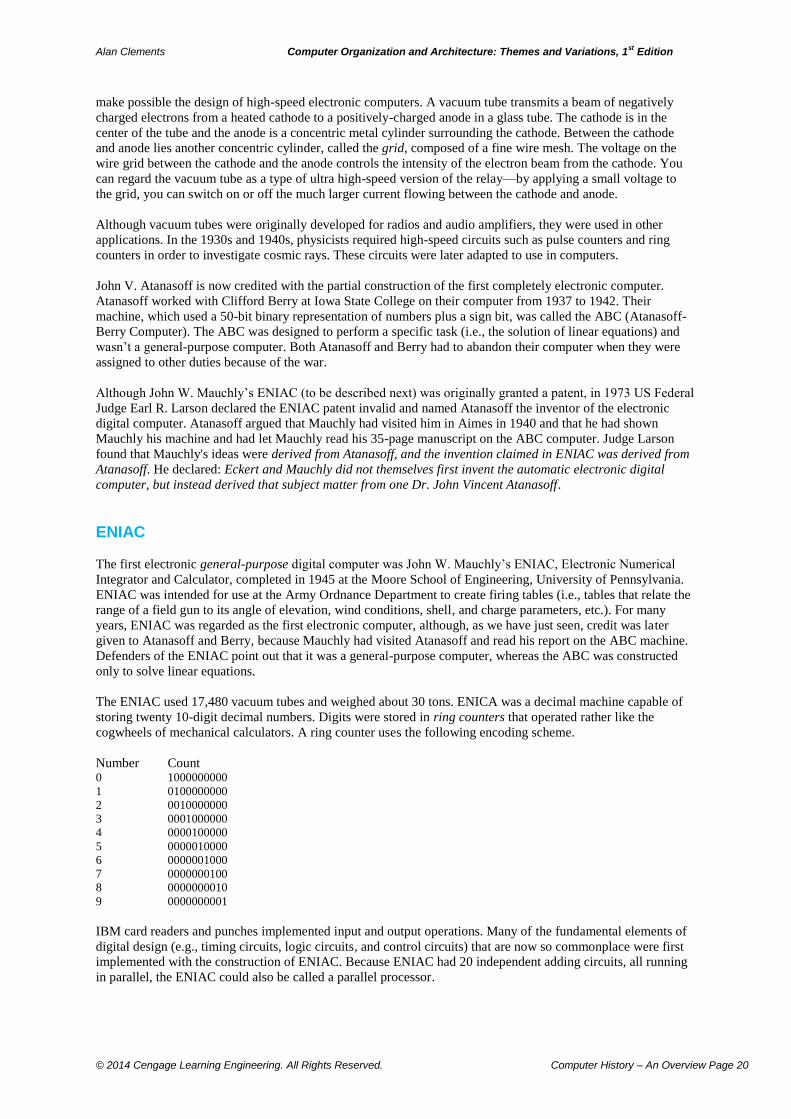
The ENIAC used 17,480 vacuum tubes and weighed about 30 tons. ENICA was a decimal machine capable of
storing twenty 10-digit decimal numbers. Digits were stored in ring counters that operated rather like the
cogwheels of mechanical calculators. A ring counter uses the following encoding scheme.
Number Count 0 1000000000
1 0100000000
2 0010000000
3 0001000000
4 0000100000
5 0000010000
6 0000001000
7 0000000100
8 0000000010
9 0000000001
IBM card readers and punches implemented input and output operations. Many of the fundamental elements of
digital design (e.g., timing circuits, logic circuits, and control circuits) that are now so commonplace were first
implemented with the construction of ENIAC. Because ENIAC had 20 independent adding circuits, all running
in parallel, the ENIAC could also be called a parallel processor.
Alan Clements Computer Organization and Architecture: Themes and Variations, 1st Edition
© 2014 Cengage Learning Engineering. All Rights Reserved. Computer History – An Overview Page 21
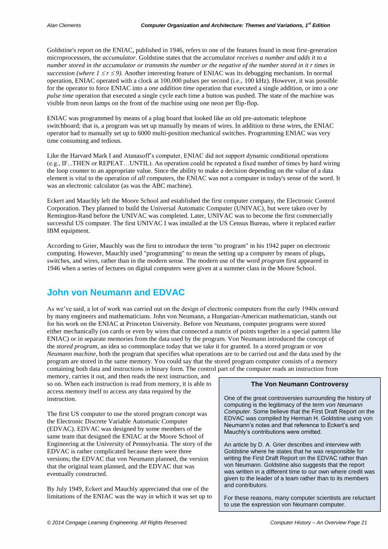
Goldstine's report on the ENIAC, published in 1946, refers to one of the features found in most first-generation
microprocessors, the accumulator. Goldstine states that the accumulator receives a number and adds it to a
number stored in the accumulator or transmits the number or the negative of the number stored in it r times in
succession (where 1 r 9). Another interesting feature of ENIAC was its debugging mechanism. In normal
operation, ENIAC operated with a clock at 100,000 pulses per second (i.e., 100 kHz). However, it was possible
for the operator to force ENIAC into a one addition time operation that executed a single addition, or into a one
pulse time operation that executed a single cycle each time a button was pushed. The state of the machine was
visible from neon lamps on the front of the machine using one neon per flip-flop.
ENIAC was programmed by means of a plug board that looked like an old pre-automatic telephone
switchboard; that is, a program was set up manually by means of wires. In addition to these wires, the ENIAC
operator had to manually set up to 6000 multi-position mechanical switches. Programming ENIAC was very
time consuming and tedious.
Like the Harvard Mark I and Atanasoff’s computer, ENIAC did not support dynamic conditional operations
(e.g., IF...THEN or REPEAT…UNTIL). An operation could be repeated a fixed number of times by hard wiring
the loop counter to an appropriate value. Since the ability to make a decision depending on the value of a data
element is vital to the operation of all computers, the ENIAC was not a computer in today's sense of the word. It
was an electronic calculator (as was the ABC machine).
Eckert and Mauchly left the Moore School and established the first computer company, the Electronic Control
Corporation. They planned to build the Universal Automatic Computer (UNIVAC), but were taken over by
Remington-Rand before the UNIVAC was completed. Later, UNIVAC was to become the first commercially
successful US computer. The first UNIVAC I was installed at the US Census Bureau, where it replaced earlier
IBM equipment.
According to Grier, Mauchly was the first to introduce the term "to program" in his 1942 paper on electronic
computing. However, Mauchly used "programming" to mean the setting up a computer by means of plugs,
switches, and wires, rather than in the modern sense. The modern use of the word program first appeared in
1946 when a series of lectures on digital computers were given at a summer class in the Moore School.
John von Neumann and EDVAC
As we’ve said, a lot of work was carried out on the design of electronic computers from the early 1940s onward
by many engineers and mathematicians. John von Neumann, a Hungarian-American mathematician, stands out
for his work on the ENIAC at Princeton University. Before von Neumann, computer programs were stored
either mechanically (on cards or even by wires that connected a matrix of points together in a special pattern like
ENIAC) or in separate memories from the data used by the program. Von Neumann introduced the concept of
the stored program, an idea so commonplace today that we take it for granted. In a stored program or von
Neumann machine, both the program that specifies what operations are to be carried out and the data used by the
program are stored in the same memory. You could say that the stored program computer consists of a memory
containing both data and instructions in binary form. The control part of the computer reads an instruction from
memory, carries it out, and then reads the next instruction, and
so on. When each instruction is read from memory, it is able to
access memory itself to access any data required by the
instruction.
The first US computer to use the stored program concept was
the Electronic Discrete Variable Automatic Computer
(EDVAC). EDVAC was designed by some members of the
same team that designed the ENIAC at the Moore School of
Engineering at the University of Pennsylvania. The story of the
EDVAC is rather complicated because there were three
versions; the EDVAC that von Neumann planned, the version
that the original team planned, and the EDVAC that was
eventually constructed.
By July 1949, Eckert and Mauchly appreciated that one of the
limitations of the ENIAC was the way in which it was set up to
The Von Neumann Controversy
One of the great controversies surrounding the history of computing is the legitimacy of the term von Neumann Computer. Some believe that the First Draft Report on the EDVAC was compiled by Herman H. Goldstine using von Neumann’s notes and that reference to Eckert’s and Mauchly’s contributions were omitted.
An article by D. A. Grier describes and interview with Goldstine where he states that he was responsible for writing the First Draft Report on the EDVAC rather than von Neumann. Goldstine also suggests that the report was written in a different time to our own where credit was given to the leader of a team rather than to its members and contributors.
For these reasons, many computer scientists are reluctant to use the expression von Neumann computer.
Alan Clements Computer Organization and Architecture: Themes and Variations, 1st Edition
© 2014 Cengage Learning Engineering. All Rights Reserved. Computer History – An Overview Page 22
solve a problem. Along with von Neumann, they realized that operating instructions should be stored in the
same memory device as the data.
By the time John von Neumann became acquainted with the ENIAC project, it was too late for him to get
involved with its design. He did participate in the EDVAC’s design and is credited with the "First Draft of a
Report on the EDVAC" that compiled the results of various design meetings. Although only von Neumann's
name appears on this document, other members of the Moore School contributed to the report. Indeed, Williams
writes that this document annoyed some members of the design team so much that they left the Moore School
and further development of the EDVAC was delayed.
The EDVAC described in von Neumann's unpublished report was a binary machine with a 32-bit wordlength.
Numbers were represented in a 31-bit signed two’s complement format and the rightmost bit was reserved as a
tag to indicate a numeric or a non-numeric value. The EDVAC that was constructed was a 44-bit machine that
didn’t use a tag bit to indicate data type. There are many other differences between the von Neumann and Moore
School EDVACs; for example, the von Neumann version had 3 registers and instructions were executed
sequentially by using a program counter to sequence them. The Moore School machine had four registers and an
instruction included a next address field (i.e., every instruction was a branch instruction). Since the memory
space was 1024 words, the instruction format called for 4 x 10-bit addresses, which left four bits to specify one
of 16 op-codes.
Although EDVAC is generally regarded as the first stored program computer, Randell states that this is not
strictly true. EDVAC did indeed store data and instructions in the same memory, but data and instructions did
not have a common format and were not interchangeable.
EDVAC also helped to promote the design of memory systems. The capacity of EDVAC's mercury delay line
memory was 1024 words of 44 bits. A mercury delay line operates by converting serial data into pulses that are
fed to an ultrasonic transducer at one end of a column of mercury in a tube. These pulses travel down the tube in
the form of ultrasonic acoustic vibrations in the mercury. A microphone at the other end of the delay line picks
up the pulses and they are regenerated into digital form. Finally, the pulses are fed back to the transducer and
sent down the delay line again. This type of memory stores data as pulses traveling through the mercury and is
no longer used. EDVAC's memory was organized as 128 individual 8-word delay lines.
Because data in a delay line memory is stored in this dynamic or sequential mode, the time taken to access an
instruction depends on where it is in the sequence of pulses. The delay lines were 58 cm long with an end-to-end
delay of 384 s. At a pulse repetition frequency of 1 MHz, each pulse had a duration of 0.3s; that is, eight 44-
bit words plus eight 4-bit interword gaps occupied 384 s. The EDVAC had the 4-address instruction format
operation source1,source2,destination,next_address
This instruction specifies the action to be carried out, the address of the two source operands, the location where
the result is to be deposited (i.e., destination), and the location of the next instruction to be executed.
The programmer would write code in such a way that the next instruction was just about to be available from the
delay line. Such code optimization techniques are not far removed from those used on modern RISC processors
to minimize the effects of data dependency and branches.
Another interesting aspect of EDVAC was the use of test routines to check its hardware; for example, the "Leap
Frog Test" executed a routine that included all its instructions, and then moved itself one location on in memory
before repeating the test. EDVAC also implemented a register that kept a copy of the last instruction executed
and its address. The operator could access this register to aid debugging when the machine crashed. Yes, the
Windows unrecoverable applications error has a very long history.
Sadly, EDVAC was not a great success in practical terms. Its construction was largely completed by April 1949,
but it didn’t run its first applications program until October 1951. Moreover, EDVAC was not very reliable and
suffered a lot of down time.
Because of its adoption of the stored program concept, EDVAC became a topic in the first lecture course given
on computers. These lectures took place before the EDVAC was actually constructed.
Alan Clements Computer Organization and Architecture: Themes and Variations, 1st Edition
© 2014 Cengage Learning Engineering. All Rights Reserved. Computer History – An Overview Page 23
IAS
An important early computer was the IAS constructed by von Neumann and his colleagues at the Institute for
Advanced Studies in Princeton. This project began in 1947 and is significant because the IAS is remarkably
similar to modern computers. The IAS supported a 40-bit word that represented data in a sign and magnitude
fixed-point format. The same wordlength was used to store two packed 20-bit instructions. Main memory was
1K words and a magnetic drum was used to provide 16K words of secondary storage. The magnetic drum was
the forerunner of today’s disk drive. Instead of recording data on the flat platter found in a hard drive, data was
stored on the surface of a rotating drum.
The IAS’s 20-bit instructions consisted of a one-address instruction of the format with an 8-bit op-code and a
12-bit address of the form
operation address
where the operation takes place between the contents of the specified memory location and the accumulator.
This format is, of course, identical to that of first generation 8-bit microprocessors. A significant feature of the
IAS was its address modify instructions that enabled you to compute a 12-bit address and then insert it into the
program as an operand. This feature enabled you to perform indexed addressing and is required to access
complex data structures such as lists, tables, and arrays. Modern architectures provide an address register or
index register to generate variable operand addresses. Modifying operands in memory the way the IAS did (self-
modifying code) is regarded as bad practice because it is error prone and makes program debugging difficult.
In the late 1940s, the first computer intended for real-time information processing was built at MIT for the US
Air Force, Whirlwind. However, its true significance was that it employed ferrite-core memory which became
the standard form of mainframe memory until the semiconductor integrated circuit came along in the late 1960s.
An Wang at Harvard University patented ferrite core memory in 1949. A ferrite core is a tiny bead of a magnetic
material that can be magnetized clockwise or counterclockwise to store a one or a zero. Ferrite core memory is
no longer widely used today, although the term remains in expressions such as core dump, which means a
printout of the contents of a region of memory.
Computers at Manchester and Cambridge Universities
In the 1940s, one of the most important centers of early computer development was Manchester University in
England where F. C. Williams used the cathode ray tube, CRT, to store binary data (2048 bits in 1947). In 1948,
T. Kilburn turned the William's memory into a prototype computer called the Manchester Baby with 32 words
of 32 bits. This was a demonstration machine that tested the concept of the stored program computer and the
Williams CRT store. CRTs were also used to implement the accumulator and logical control. Input was read
directly from switches and output had to be read from the William's tube. The first program to run on the
machine was designed to find the highest factor of an integer. Some regard the Manchester Baby as the world's
first stored-program computer. A Manchester-based firm, Ferranti Ltd., worked with Manchester University to
construct Manchester University's first practical computer, the Ferranti Mark I.
Maurice V. Wilkes at the University of Cambridge built another early computer, the Electronic Delay Storage
Automatic Calculator, EDSAC. This became operational in May 1949, used paper tape input, binary numbers,
and mercury delay line storage. Like the IAS, EDSAC allowed you to modify instructions in order to implement
indexed addressing.
Scientists sometimes make startlingly incorrect prophecies; for example, the British Astronomer Royal said,
Space travel is bunk just before the USSR launched its first sputnik. Similarly, not everyone immediately
appreciated the potential of the computer. In 1951, Professor Hartree at Cambridge University said, "We have a
computer in Cambridge; there is one in Manchester and at the NPL. I suppose that there ought to be one in
Scotland, but that's about all.”
Cooperation between Ferranti and Manchester University led to the development of the Ferranti Mercury that
pioneered the use of floating-point arithmetic and replaced the Williams CRT by ferrite core memory. In true
British tradition, the Ferranti computers had considerable technical merit, but lacked many important
commercial features required for their economic success, such as a punched card reader.
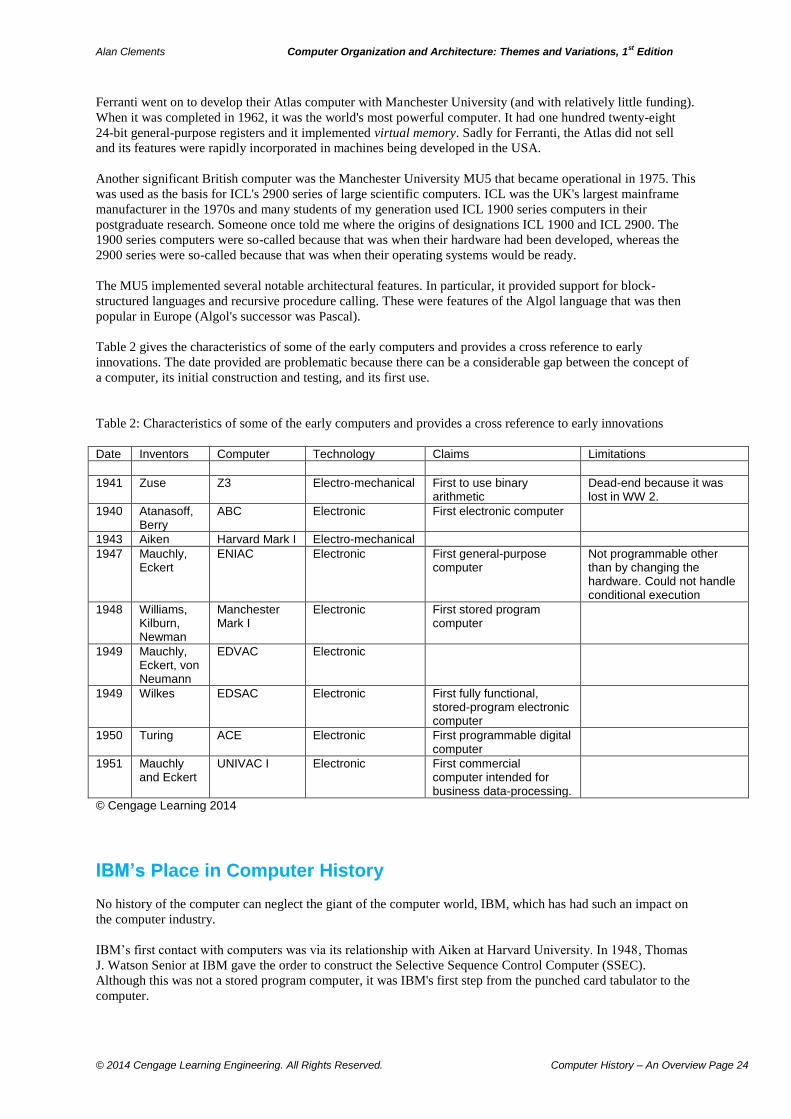
Alan Clements Computer Organization and Architecture: Themes and Variations, 1st Edition
© 2014 Cengage Learning Engineering. All Rights Reserved. Computer History – An Overview Page 24
Ferranti went on to develop their Atlas computer with Manchester University (and with relatively little funding).
When it was completed in 1962, it was the world's most powerful computer. It had one hundred twenty-eight
24-bit general-purpose registers and it implemented virtual memory. Sadly for Ferranti, the Atlas did not sell
and its features were rapidly incorporated in machines being developed in the USA.
Another significant British computer was the Manchester University MU5 that became operational in 1975. This
was used as the basis for ICL's 2900 series of large scientific computers. ICL was the UK's largest mainframe
manufacturer in the 1970s and many students of my generation used ICL 1900 series computers in their
postgraduate research. Someone once told me where the origins of designations ICL 1900 and ICL 2900. The
1900 series computers were so-called because that was when their hardware had been developed, whereas the
2900 series were so-called because that was when their operating systems would be ready.
The MU5 implemented several notable architectural features. In particular, it provided support for block-
structured languages and recursive procedure calling. These were features of the Algol language that was then
popular in Europe (Algol's successor was Pascal).
Table 2 gives the characteristics of some of the early computers and provides a cross reference to early
innovations. The date provided are problematic because there can be a considerable gap between the concept of
a computer, its initial construction and testing, and its first use.
Table 2: Characteristics of some of the early computers and provides a cross reference to early innovations
Date Inventors Computer Technology Claims Limitations
1941 Zuse Z3 Electro-mechanical First to use binary arithmetic
Dead-end because it was lost in WW 2.
1940 Atanasoff, Berry
ABC Electronic First electronic computer
1943 Aiken Harvard Mark I Electro-mechanical
1947 Mauchly, Eckert
ENIAC Electronic First general-purpose computer
Not programmable other than by changing the hardware. Could not handle conditional execution
1948 Williams, Kilburn, Newman
Manchester Mark I
Electronic First stored program computer
1949 Mauchly, Eckert, von Neumann
EDVAC Electronic
1949 Wilkes EDSAC Electronic First fully functional, stored-program electronic computer
1950 Turing ACE Electronic First programmable digital computer
1951 Mauchly and Eckert
UNIVAC I Electronic First commercial computer intended for business data-processing.
© Cengage Learning 2014
IBM’s Place in Computer History
No history of the computer can neglect the giant of the computer world, IBM, which has had such an impact on
the computer industry.
IBM’s first contact with computers was via its relationship with Aiken at Harvard University. In 1948, Thomas
J. Watson Senior at IBM gave the order to construct the Selective Sequence Control Computer (SSEC).
Although this was not a stored program computer, it was IBM's first step from the punched card tabulator to the
computer.
Alan Clements Computer Organization and Architecture: Themes and Variations, 1st Edition
© 2014 Cengage Learning Engineering. All Rights Reserved. Computer History – An Overview Page 25
IBM under T. J. Watson Senior didn’t wholeheartedly embrace the computer revolution in its early days.
However, T. J. Watson, Jr., was responsible for building the Type 701 Electronic Data Processing Machine
(EDPM) in 1953 to convince his father that computers were not a threat to IBM's conventional business. Only
nineteen models of this binary fixed-point machine that used magnetic tape to store data were built. However,
the 700 series was successful and dominated the mainframe market for a decade and, by the 1960s, IBM was the
most important computer manufacturer in the world. In 1956, IBM launched a successor, the 704 that was the
world's first super-computer and the first machine to incorporate floating-point hardware (if you are willing to
forget Zuse’s contribution). The 704 was largely designed by Gene Amdahl who later founded his own
supercomputer company in the 1990s.
Although IBM’s 700 series computers were incompatible with their punched card processing equipment, IBM
created the 650 EDPM that was compatible with the 600 series calculators and used the same card processing
equipment. This provided an upward compatibility path for existing IBM users, a process that was later to
become commonplace in the computer industry.
IBM’s most important mainframe was the 32-bit System/360, first delivered in 1965 and designed to suit both
scientific and business applications. The importance of the System/360 is that it was a member of series of
computers, each with the same architecture (i.e., programming model), but with different performance; for
example, the System/360 model 91 was 300 times
faster than the model 20. Each member of the
System/360 was software compatible with all other
members of the same series. IBM also developed a
common operating system, OS/360, for their series.
Other manufacturers built their own computers that
were compatible with System/360 and thereby began
the slow process towards standardization in the
computer industry. Incidentally, prior to the
System/360, a byte referred to a 6-bit quantity rather
than an 8-bit value.
An interesting feature of the System/360 was its ability
to run the operating system in a protected state, called
the supervisor state. Applications programs running
under the operating system ran in the user state. This
feature was later adopted by Motorola’s 680x0
microprocessor series.
In 1960, the Series/360 model 85 became the first
computer to implement cache memory, a concept
described by Wilkes in 1965. Cache memory keeps a
copy of frequently used data in very high-speed
memory to reduce the number of accesses to the slower
main store. Cache memory has become one of the most
important features of today’s high performance systems. By the early 1970s, the Series/360 had evolved to
include the virtual memory technology first used in the Manchester Atlas machine.
IBM introduced one of the first computers to use integrated circuits, ICs, in the 1970s. This was the System/370
that could maintain backward compatibility by running System/360 programs.
In August 1980, IBM became the first major manufacturer to market a personal computer. IBM had been
working on a PC since about 1979, when it was becoming obvious that IBM’s market would eventually start to
come under threat from the newly emerging personal computer manufacturers, such as Apple and Commodore.
Although IBM is widely known by the general public for its mainframes and personal computers, IBM invented
introduced the floppy disk, computerized supermarket checkouts, and the first automatic teller machines.
We now take a slight deviation into microprogramming, a technique that had a major impact on the architecture
and organization of computers in the 1960s and 1970s. Microprogramming was used to provide members of the
System/360 series with a common architecture.
IBM’s Background IBM’s origin dates back to the 1880s. The CTR Company was the result of a merger between the International Time Recording Company (ITR), the Computing Scale Company of America, and Herman Hollerith's Tabulating Machine Company (founded in 1896). ITR was founded in 1875 by clock maker Willard Bundy who designed a mechanical time recorder. CTR was a holding company for other companies that produced components or finished products; for example, weighing and measuring machines, time recorders, tabulating machines with punch cards. In 1914, Thomas J. Watson, Senior, left the National Cash Register Company to join CTR and soon became president. In 1917, a Canadian unit of CTR called International Business Machines Co. Ltd was set up. Because this name was so well suited to CTR's role, they adopted this name for the whole organization in 1924. In 1928, the capacity of a punched card was increased from 45 to 80 columns. IBM bought Electromatic Typewriters in 1933 and the first IBM electric typewriter was marketed two years later. Although IBM's principal product was punched card processing equipment, after the 1930s IBM produced their 600 series calculators.
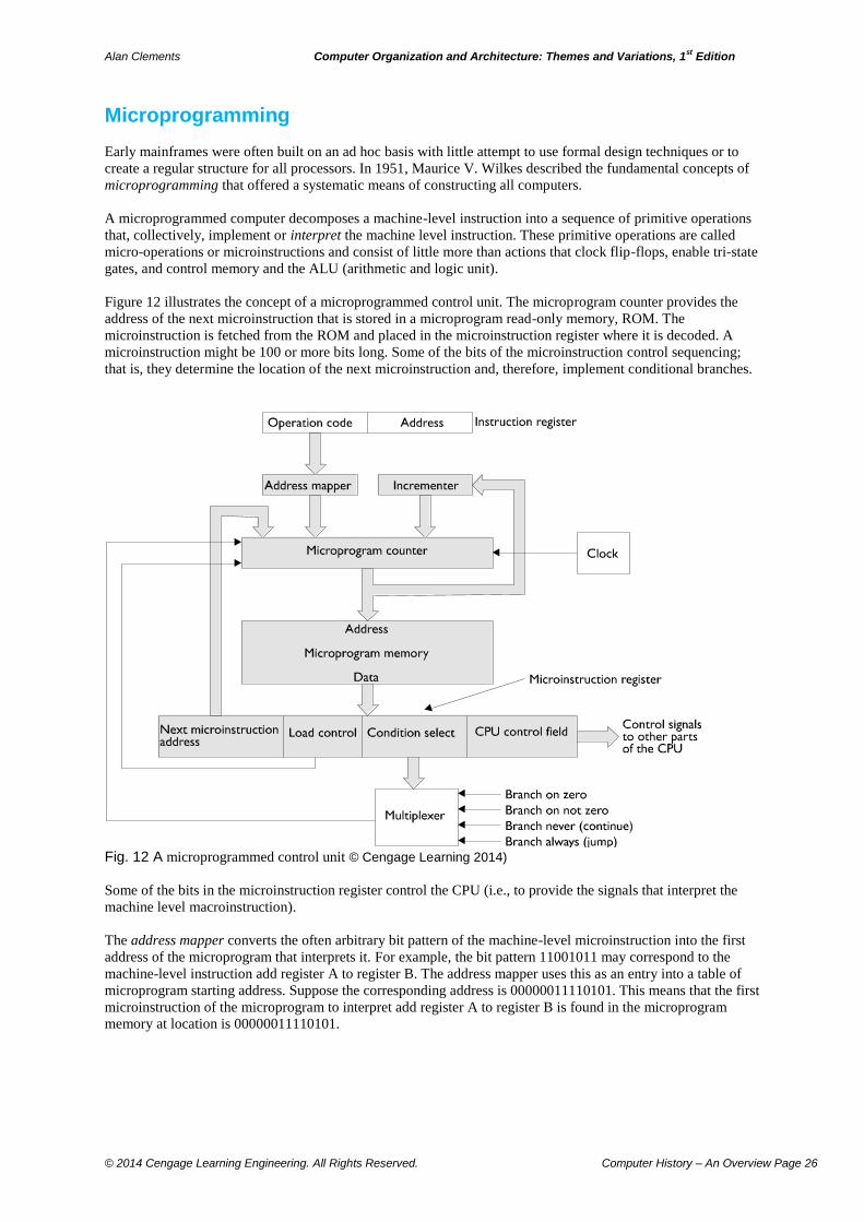
Alan Clements Computer Organization and Architecture: Themes and Variations, 1st Edition
© 2014 Cengage Learning Engineering. All Rights Reserved. Computer History – An Overview Page 26
Microprogramming
Early mainframes were often built on an ad hoc basis with little attempt to use formal design techniques or to
create a regular structure for all processors. In 1951, Maurice V. Wilkes described the fundamental concepts of
microprogramming that offered a systematic means of constructing all computers.
A microprogrammed computer decomposes a machine-level instruction into a sequence of primitive operations
that, collectively, implement or interpret the machine level instruction. These primitive operations are called
micro-operations or microinstructions and consist of little more than actions that clock flip-flops, enable tri-state
gates, and control memory and the ALU (arithmetic and logic unit).
Figure 12 illustrates the concept of a microprogrammed control unit. The microprogram counter provides the
address of the next microinstruction that is stored in a microprogram read-only memory, ROM. The
microinstruction is fetched from the ROM and placed in the microinstruction register where it is decoded. A
microinstruction might be 100 or more bits long. Some of the bits of the microinstruction control sequencing;
that is, they determine the location of the next microinstruction and, therefore, implement conditional branches.
Fig. 12 A microprogrammed control unit © Cengage Learning 2014)
Some of the bits in the microinstruction register control the CPU (i.e., to provide the signals that interpret the
machine level macroinstruction).
The address mapper converts the often arbitrary bit pattern of the machine-level microinstruction into the first
address of the microprogram that interprets it. For example, the bit pattern 11001011 may correspond to the
machine-level instruction add register A to register B. The address mapper uses this as an entry into a table of
microprogram starting address. Suppose the corresponding address is 00000011110101. This means that the first
microinstruction of the microprogram to interpret add register A to register B is found in the microprogram
memory at location is 00000011110101.
Alan Clements Computer Organization and Architecture: Themes and Variations, 1st Edition
© 2014 Cengage Learning Engineering. All Rights Reserved. Computer History – An Overview Page 27
A microprogrammed control unit can be used to implement any digital machine. In order to implement the
control unit of any arbitrary architecture, all that you have to change is the microprogram itself and the structure
of the CPU control field.
Without microprogramming, a computer has to be constructed from digital circuits that are designed to execute
the machine code instructions. Such a design is specific to a particular architecture and organization.
Microprogramming offers a general technique that can be applied to any computer; for example, you could
construct a microprogrammed control unit that is capable of implementing, say, the Intel IA32 instruction set,
the ARM processor’s instruction set, the PowerPC instruction set, or even the ENIAC’s instruction set.
Because the microprogrammed control unit is such a regular structure, it was possible to develop formal
methods for the design of microprograms and to construct tools to aid the creation, validation, and testing of
microprograms. Microprogramming also made it relatively easy to include self-diagnostic tools in the
microcode. The body of knowledge associated with microprogramming became known as firmware
engineering.
The historical significance of microprogramming is its role in separating architecture and organization. Prior to
the introduction of microprogramming, there was no real difference between architecture and organization,
because a computer was built to directly implement its architecture. Microprogramming made it possible to
divorce architecture from organization. By means of a suitable microprogram you could implement any
architecture on the simplest of CPUs.
In practical terms, a company could design a powerful architecture that, for example, supported high-level
languages and operating systems, and then use microprogramming to implement this architecture on a range of
machines. Such an approach allows you to select the most cost-effective system for your specific application. A
high-end system might use a hardware floating-point unit, whereas a lower cost system might interpret floating-
point operations in microcode. Both these systems run the same source code, the only difference being the
performance of the computer.
The microprogram store is a read-only memory because the microcode is fixed. In the mid-1970s it became
obvious that, by employing a writable microprogram control store, users could implement their own instruction
sets or even dynamically change the architecture of the computer. By changing your architecture, you could still
run your old programs on your new microprogrammed machine by emulating the old architecture in microcode.
Machine emulation was very important at a time when computers cost hundreds of thousands of dollars and the
software base was very small. Microprogramming made it possible to close the semantic gap and even directly
execute high-level languages. For a time in the 1970s, it seemed like that microprogramming was the new
solution to all problems.
By the late 1970s, companies like AMD were fabricating integrated circuits that made it easy to construct
microprogrammed control units. These devices, that also included ALUs and register files, were called bit slice
chips because they were 4 bits wide and you could wire several chips together to construct a system with any
wordlength that was a multiple of 4 bits.
In 1980, two engineers at AMD with the improbable names Mick and Brick published Bit-slice Microprocessor
Design, an impressive book that discussed the design of microprogrammed computers using AMD’s devices.
They went into considerable practical detail about microprogrammed systems and enabled anyone with a
modest computer engineering background to design their own architecture and implement it. Just as all fiction
writers dream of writing the Great American Novel, all computer engineers dreamt of building their own
microprocessor with their own instruction set.
The rise of microprogrammed bit slice architectures coincided with the introduction of 16- and 32-bit
microprocessors like the 68000. With such affordable computing power, the pressure to build your own
microprocessor rapidly diminished. Although the idea of microprogramming, writable control store and bit slice
computers was very exciting at the time, it was horribly impractical. If you create your own architecture, you are
denied the software available to those using mainstream commercial devices. That was not too bad in the early
1970s, because very little commercial software was available. Once operating systems, compilers, word
processors, and spreadsheets, etc., became widely available for popular microprocessors, the appeal of
microprogramming for the masses rapidly diminished.
Alan Clements Computer Organization and Architecture: Themes and Variations, 1st Edition
© 2014 Cengage Learning Engineering. All Rights Reserved. Computer History – An Overview Page 28
Microprogramming was still used by microprocessor manufacturers to implement CPUs; for example,
Motorola’s 16/32-bit 68000 microprocessor was one of the first microprocessors to have a microprogrammed
control unit. Even Intel’s IA32 still employs microprogramming to implement some instructions.
User-configurable microprogramming was doomed. An advantage of microprogrammed architectures was their
flexibility and ease of implementation. Another advantage was their efficient use of memory. In 1970, main
store random access memory was both slow and expensive. The typical access time of ferrite core memory was
1 s. By implementing complex-instruction architectures an interpreting the instructions in microcode, the size
of programs could be reduced to minimize the requirements of main memory. The control store was much faster
than the main memory and it paid to implement complex machine-level instructions in microcode.
By the 1980s, the cost of memory had dramatically reduced and its access time had fallen to 100 ns. Under such
circumstances, the microprogrammed architecture lost its appeal. Moreover, a new class of highly efficient non-
microprogrammed architectures arose in the 1980s called RISC processors (reduced instruction set computers).
You could almost consider RISC processors computers where the machine-level code was, essentially, the same
as microcode.
Microprogramming has come and gone, although some of today’s complex processors still use microcode to
execute some of their more complex instructions. It enabled engineers to implement architectures in a painless
fashion and was responsible for ranges of computers that shared a common architecture but different
organizations and performances. Such ranges of computer allowed companies like IBM and DEC to dominate
the computer market and to provide stable platforms for the development of software. The tools and techniques
used to support microprogramming provided a basis for firmware engineering and helped expand the body of
knowledge that constituted computer science.
The Birth of Transistors and ICs
Since the 1940s, computer hardware has become smaller and smaller and faster and faster. The power-hungry
and unreliable vacuum tube was replaced by the much smaller and more reliable transistor in the 1950s. The
transistor, invented by William Shockley, John Bardeen, and Walter Brattain at AT&T’s Bell Lab in 1947, plays
the same role as a thermionic tube. The only real
difference is that a transistor switches a current
flowing through a crystal rather than a beam of
electrons flowing through a vacuum. Transistors are
incomparably more reliable than vacuum tubes and
consume a tiny fraction of their power (remember that
a vacuum tube has a heated cathode).
If you can put one transistor on a slice of silicon, you
can put two or more transistors on the same piece of
silicon. The integrated circuit (IC), a complete
functional unit on a single chip, was an invention
waiting to be made. The idea occurred to Jack St. Clair
Kilby at Texas Instruments in 1958 who built a
working model and filed a patent early in 1959.
However, in January of 1959, Robert Noyce at
Fairchild Semiconductor was also thinking of the
integrated circuit. He too applied for a patent and it
was granted in 1961. Today, both Noyce and Kilby are
regarded as the joint inventors of the IC.
By the 1970s, entire computers could be produced on a single silicon chip. The progress of electronics has been
remarkable. Today you can put over 2,000,000,000 transistors in the same space occupied by a tube in 1945. If
human transport had evolved at a similar rate, and we assume someone could travel at 20 mph in 1900, we
would be able to travel at 40,000,000,000 mph today (i.e., about 200,000 times the speed of light!).
Who Invented the Transistor? It is traditional to ascribe the invention of the transistor to the team at Bell Labs. As in most cases of engineering innovation, the story is not so simple. Julius Edgar Lilienfeld filed a patent for what would today be called a field effect transistor in 1925. Another German inventor, Oskar Heil, also filed a British patent describing a field effect transistor in 1935. In 1947, two German physicists, Mataré and Welker independently invented the point-contact transistor in Paris. First-generation transistors used germanium as a semiconductor. It wasn’t until 1954 that the first silicon transistor was produced by Texas Instruments. The form of transistor found in today’s integrated circuits is the metal oxide field-effect transistor, MOSFET, was invented by Kahng and Atalla at Bell Labs in 1959. This operates on the same principles described by Lilienfeld a quarter of a century earlier.
Alan Clements Computer Organization and Architecture: Themes and Variations, 1st Edition
© 2014 Cengage Learning Engineering. All Rights Reserved. Computer History – An Overview Page 29
Final Thoughts on the Invention of the Computer
So, who did invent the computer? By now you should appreciate that this is, essentially, a meaningless question.
Over a long period, people attempted to design and construct calculating machines. As time passed more and
more enabling technologies were developed and computer-like machines began to emerge in the 1940s. These
machines had some of, but not all, the attributes of machines that we now call a computer. Some lacked the
stored program concept; others lacked the ability to handle conditional operations, and so on. It seems to me
unfair to declare that any one of these machines was the first computer.
It seems that we always like to associate a specific person with an invention. From 1950, Mauchly and Eckert
shared the original computer patent rights because of their work on the ENIAC. However, in 1973 Judge Larson
in Minneapolis presided over the controversial lawsuit brought by Sperry Rand against Honeywell Incorporated
for patent infringement. Judge Larson ruled that John Atanasoff should be credited with the invention of the
computer, and that the Mauchly and Eckert patent was invalid because Atanasoff met John Mauchly at a
conference in 1940 and discussed his work at Iowa State with Mauchly. Furthermore, Mauchly visited Atanasoff
and looked at his notes on his work.
Had these computers not been developed, modern computing might have taken a different path. However, the
computing industry would probably have ended up not too far from today's current state.
Table 3 provides a timescale that includes some of the key stages in the development of the computer. Some of
the dates are approximate because an invention can be characterized by the date the inventor began working on
it, the date on which the invention was first publicly described or patented, the date on which it was
manufactured, the date on which they got it working, or the date on which the inventor stopped working on it.
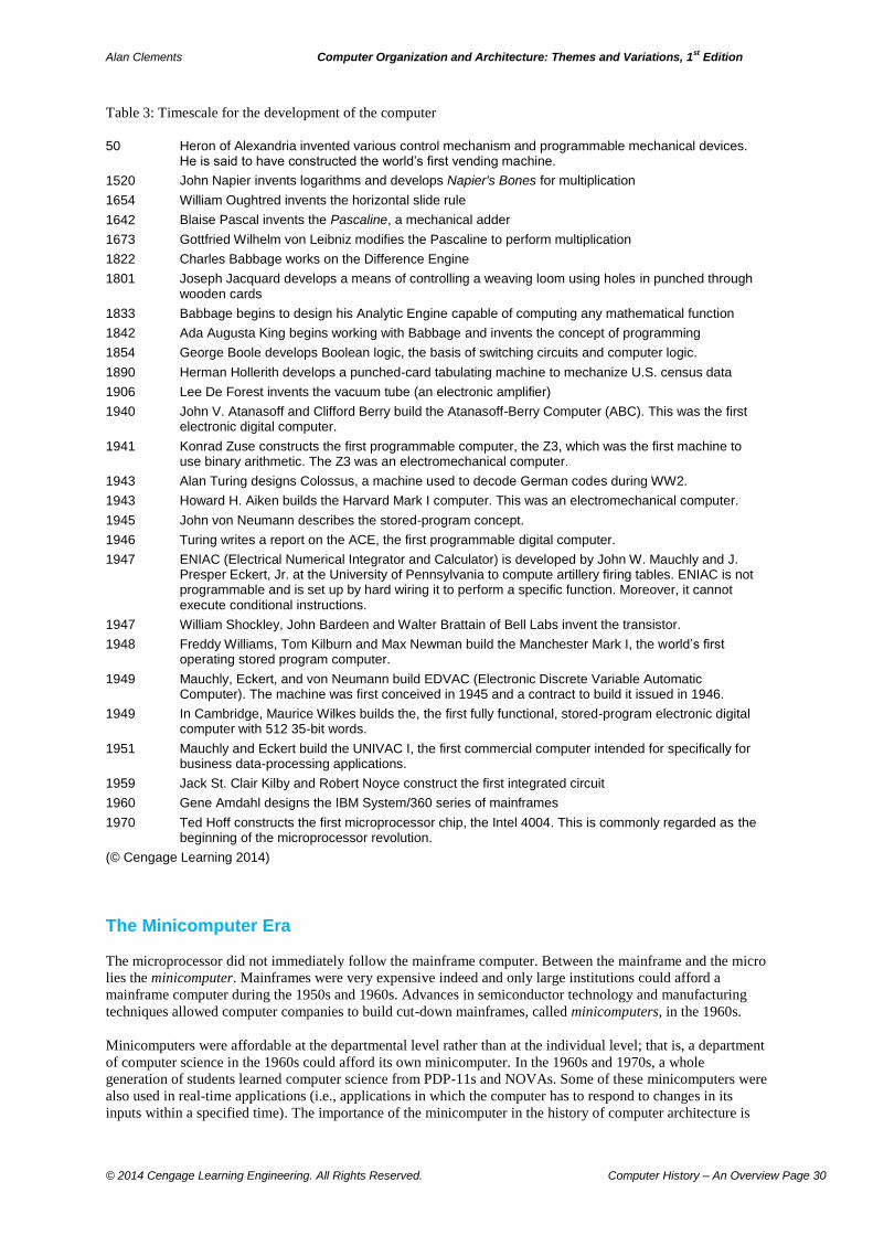
Alan Clements Computer Organization and Architecture: Themes and Variations, 1st Edition
© 2014 Cengage Learning Engineering. All Rights Reserved. Computer History – An Overview Page 30
Table 3: Timescale for the development of the computer
50 Heron of Alexandria invented various control mechanism and programmable mechanical devices.
He is said to have constructed the world’s first vending machine.
1520 John Napier invents logarithms and develops Napier's Bones for multiplication
1654 William Oughtred invents the horizontal slide rule
1642 Blaise Pascal invents the Pascaline, a mechanical adder
1673 Gottfried Wilhelm von Leibniz modifies the Pascaline to perform multiplication
1822 Charles Babbage works on the Difference Engine
1801 Joseph Jacquard develops a means of controlling a weaving loom using holes in punched through wooden cards
1833 Babbage begins to design his Analytic Engine capable of computing any mathematical function
1842 Ada Augusta King begins working with Babbage and invents the concept of programming
1854 George Boole develops Boolean logic, the basis of switching circuits and computer logic.
1890 Herman Hollerith develops a punched-card tabulating machine to mechanize U.S. census data
1906 Lee De Forest invents the vacuum tube (an electronic amplifier)
1940 John V. Atanasoff and Clifford Berry build the Atanasoff-Berry Computer (ABC). This was the first electronic digital computer.
1941 Konrad Zuse constructs the first programmable computer, the Z3, which was the first machine to use binary arithmetic. The Z3 was an electromechanical computer.
1943 Alan Turing designs Colossus, a machine used to decode German codes during WW2.
1943 Howard H. Aiken builds the Harvard Mark I computer. This was an electromechanical computer.
1945 John von Neumann describes the stored-program concept.
1946 Turing writes a report on the ACE, the first programmable digital computer.
1947 ENIAC (Electrical Numerical Integrator and Calculator) is developed by John W. Mauchly and J. Presper Eckert, Jr. at the University of Pennsylvania to compute artillery firing tables. ENIAC is not programmable and is set up by hard wiring it to perform a specific function. Moreover, it cannot execute conditional instructions.
1947 William Shockley, John Bardeen and Walter Brattain of Bell Labs invent the transistor.
1948 Freddy Williams, Tom Kilburn and Max Newman build the Manchester Mark I, the world’s first operating stored program computer.
1949 Mauchly, Eckert, and von Neumann build EDVAC (Electronic Discrete Variable Automatic Computer). The machine was first conceived in 1945 and a contract to build it issued in 1946.
1949 In Cambridge, Maurice Wilkes builds the, the first fully functional, stored-program electronic digital computer with 512 35-bit words.
1951 Mauchly and Eckert build the UNIVAC I, the first commercial computer intended for specifically for business data-processing applications.
1959 Jack St. Clair Kilby and Robert Noyce construct the first integrated circuit
1960 Gene Amdahl designs the IBM System/360 series of mainframes
1970 Ted Hoff constructs the first microprocessor chip, the Intel 4004. This is commonly regarded as the beginning of the microprocessor revolution.
(© Cengage Learning 2014)
The Minicomputer Era
The microprocessor did not immediately follow the mainframe computer. Between the mainframe and the micro
lies the minicomputer. Mainframes were very expensive indeed and only large institutions could afford a
mainframe computer during the 1950s and 1960s. Advances in semiconductor technology and manufacturing
techniques allowed computer companies to build cut-down mainframes, called minicomputers, in the 1960s.
Minicomputers were affordable at the departmental level rather than at the individual level; that is, a department
of computer science in the 1960s could afford its own minicomputer. In the 1960s and 1970s, a whole
generation of students learned computer science from PDP-11s and NOVAs. Some of these minicomputers were
also used in real-time applications (i.e., applications in which the computer has to respond to changes in its
inputs within a specified time). The importance of the minicomputer in the history of computer architecture is
Alan Clements Computer Organization and Architecture: Themes and Variations, 1st Edition
© 2014 Cengage Learning Engineering. All Rights Reserved. Computer History – An Overview Page 31
that it provided a template for its successor, the microprocessor. That is, microprocessor architectures looked
much more like minicomputer architectures than mainframes.
It is interesting to read the definition of a minicomputer made by Kraft and Toy in 1970:
A minicomputer is a small, general-purpose, stored program digital computer that:
1. has a word length ranging from 8 bits to 32 bits.
2. provides at least 4096 words of program memory.
3. sells for under $20,000 in a minimum usable configuration, consisting of a teletypewriter, a power
supply, and a front panel to be used as a programmer’s console.
One of the first minicomputers was Digital Equipment Corporation’s 12-bit PDP-5, which was introduced in
1964. This was followed by the PDP-8 in 1966, which also had a 12-bit wordlength and could address 212
=
4,096 memory locations. By using two 3-bit segment registers, the address space could be increased to two sets
of 28 = 8 pages of 4 K words. One segment register was used to access program space and one was used to
access data space. Later, the Intel 8086 family was to adopt a similar form of segmented addressing.
The PDP-8 had a single 12-bit accumulator and provided a very basic instruction set including addition,
subtraction, data movement, Boolean operations, and shifts. Program control instructions were of the form skip
on condition, where condition was limited to negative, positive, zero, and not zero accumulator (plus two skip
operations dependent on the state of the accumulator’s link bit). An important feature of the PDP-8 was its eight
12-bit index registers that were located in memory. These registers were auto-incrementing and the contents of
an index register were incremented whenever it was used to access data.
The principal limitations of the PDP-8 were its lack of registers, its lack of hardware support for a stack pointer,
its lack of byte-oriented instructions, and its lack of interrupt prioritization. The PDP-8’s relatively primitive
architecture led DEC to design a more sophisticated successor, the PDP-11, in 1969.
Because of its byte-oriented 16-bit architecture, the PDP-11 was better suited to text processing applications
than the PDP-8. The PDP-11 has eight 16-bit general-purpose registers, R0 to R7 and looked very much like the
second-generation microprocessors that would appear in under a decade. An important feature of the PDP-11
was the UNIBUS, a data highway used by the CPU to communicate with memory and peripherals. The
UNIBUS used an asynchronous protocol to allow data transfers to take place at a rate determined by the
characteristics of the bus slave being accessed. A later model, the PDP-11/70, implemented a dedicated bus
between its cache and CPU because the UNIBUS was too slow for memory traffic. Adding a dedicated bus to
get round technology problems when a standard bus began to grow obsolete was also a feature of the
development of the IBM PC.
DEC built on their success with the PDP-11 series and introduced their VAX architecture in 1978 with the
VAX-11/780. The VAX had a 32-bit architecture and was available in a range of models. Microprogramming
was used to implement its control unit. The VAX dominated the minicomputer world in the 1980s and was
sometimes called a superminicomputer. DEC replaced VAX by the 64-bit Alpha architecture (a high
performance microprocessor) in 1991. Sadly, DEC went from being one of the rising stars of the new computer
world to a footnote in computer history when it was sold off to Compaq in 1998. Compaq’s acquisition was not
successful and Compaq itself was absorbed by Hewlett-Packard in 2002.
It would be wrong to suggest that DEC was the only minicomputer manufacturer. There were several other
major players in the minicomputer market. For example, Data General produced its Nova range of computers in
the late 1960s and announced its Eclipse series of minicomputers in 1974. Hewlett-Packard’s HP2100 series
was another significant range of minicomputers, not least because of its use of microprogramming.
We next look at the development of the device that was to trigger the microprocessor revolution of the 1970s.
Birth of the Microprocessor: From 4004 to Golden Age
Before we describe the birth of the microprocessor, we need to briefly introduce the integrated circuit that made
the microprocessor possible. The transistor operates by controlling the flow of electrons through a
semiconductor. When the transistor was first invented, the semiconducting element used to fabricate it was
germanium, whereas today most transistors are made from silicon. A transistor is composed of nothing more
Alan Clements Computer Organization and Architecture: Themes and Variations, 1st Edition
© 2014 Cengage Learning Engineering. All Rights Reserved. Computer History – An Overview Page 32
than adjoining regions of silicon doped with different concentrations of impurities. These impurities are atoms
of elements like boron, phosphorous, and arsenic. Combining silicon with oxygen creates silicon dioxide, SiO2,
a powerful insulator that allows you to separate regions of differently doped silicon. Electrical contacts are made
by evaporating (or sputtering) aluminum on to the surface of a silicon chip. In other words, an integrated circuit
is made simply by modifying the properties of atoms in a semiconductor and by adding conducting and
insulating layers.
Not only is the transistor a tiny device, it is manufactured by fully automated techniques. The basic fabrication
process involves covering the silicon with a photosensitive layer. Then an image is projected onto the
photosensitive layer and developed to selectively remove parts of the photosensitive layer. The silicon is then
heated in an atmosphere containing the impurities used to dope the silicon, and the impurities diffuse into the
surface to change the silicon’s electrical properties. This entire sequence is repeated several times to build up
layers with different types of doping material, and then insulators and conductors created.
As manufacturing technology evolved, more and more transistors were fabricated on single silicon chips with
the maximum number of transistors per chip doubling every year between 1961 and 1971. The basic functional
units evolved from simple gates to arithmetic units, small memories, and special-purpose functions such as
multiplexers and decoders. In 1967, Fairchild introduced an 8-bit ALU chip that included its own accumulator.
It was inevitable that someone would eventually invent the microprocessor because, by the late 1960s,
computers built from discrete transistors and simple integrated circuits already existed. Integrated circuits were
getting more and more complex day by day and only one step remained, putting everything together on one
chip. The only real issue was when a semiconductor manufacturer would decide that a general-purpose digital
computer was worth developing economically.
The Intel 4004
Credit for creating the world's first microprocessor, the Intel 4040, goes to Ted Hoff and Federico Faggin,
although William Aspray in the Annals of the History of Computing points out that the microprocessor's
development was a more complex and interesting story than many realize. In 1969, Bob Noyce and Gordon
Moore set up the Intel Corporation to produce semiconductor memory chips for the mainframe industry. A year
later Intel began to develop a set of calculator chips for a consortium of two Japanese companies. These chips
were to be used in the Busicom range of calculators.
Three engineers from Japan worked with M. E. Hoff at Intel to implement the calculator's digital logic circuits
in silicon. Hoff had a Ph.D. from Stanford University and a background in the design of interfaces for several
IBM computers. When Hoff studied the calculator's logic, he was surprised by its complexity (in contrast to the
general-purpose circuits in digital computers). Hoff thought that the calculator was too complex and that the
packaging issues raised by the use of seven different large scale integration chips were severe.
Bob Noyce encouraged Hoff to look at the design of the calculator. One of Hoff's major contributions was to
replace the complex and slow shift registers used to store data in the calculator with the DRAM memory cells
that Intel was developing as storage elements. This step provided the system with more and faster memory. Hoff
also suggested adding subroutine calls to the calculator's instruction set in order to reduce the amount of
hardwired logic in the system.
These ideas convinced Hoff to go further and develop a general-purpose computer that could be programmed to
carry out calculator functions. By the end of 1969, Stanley Mazor, who also had computer design experience,
joined the development team. Mazor added a fetch indirect instruction and (with Shima) coded an interpreter to
execute 1-byte macroinstructions. Shima also proposed including a conditional jump based on the status of an
external pin.
Towards the end of 1969, the structure of a programmable calculator had emerged and Intel and Busicom chose
the programmable calculator in preference to Busicom's original model. However, the project was delayed until
Fredrico Faggin joined Intel in 1970 and helped transform the logic designs into silicon. In order to create a chip
of such complexity, Faggin had to develop new semiconductor design technologies. The 4004 used about 2300
transistors and is considered the first general-purpose programmable microprocessor, even though it was only a
4-bit device.
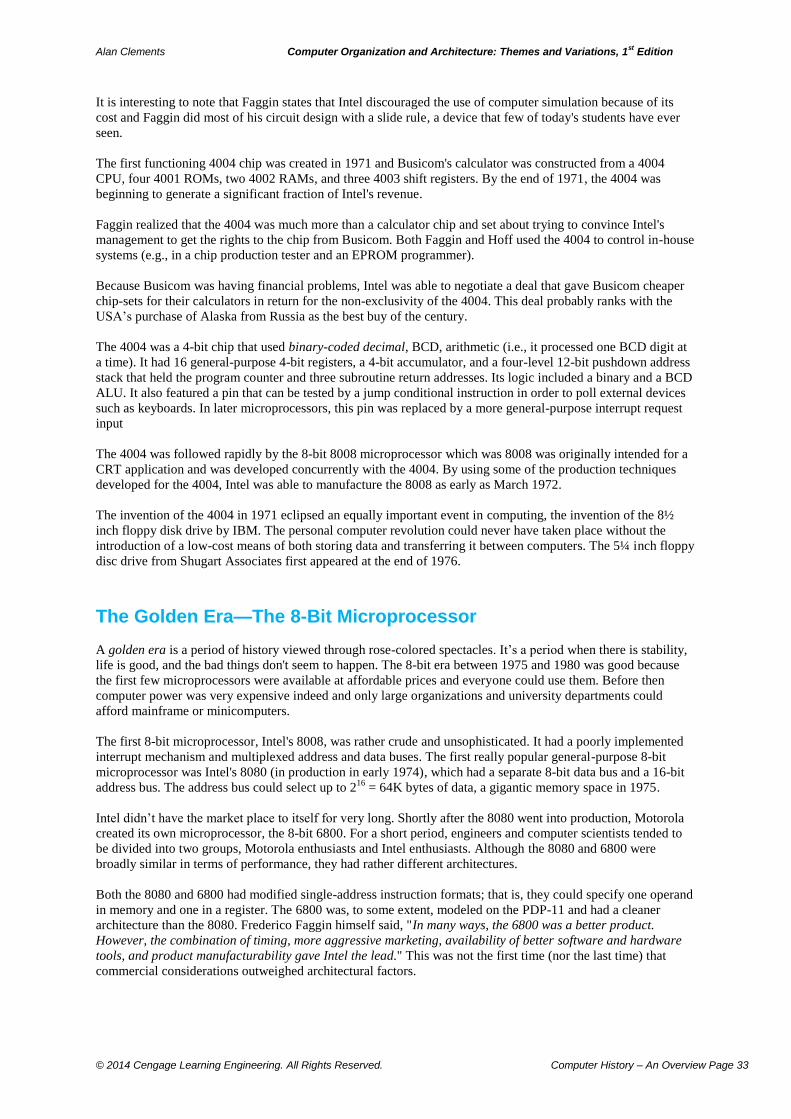
Alan Clements Computer Organization and Architecture: Themes and Variations, 1st Edition
© 2014 Cengage Learning Engineering. All Rights Reserved. Computer History – An Overview Page 33
It is interesting to note that Faggin states that Intel discouraged the use of computer simulation because of its
cost and Faggin did most of his circuit design with a slide rule, a device that few of today's students have ever
seen.
The first functioning 4004 chip was created in 1971 and Busicom's calculator was constructed from a 4004
CPU, four 4001 ROMs, two 4002 RAMs, and three 4003 shift registers. By the end of 1971, the 4004 was
beginning to generate a significant fraction of Intel's revenue.
Faggin realized that the 4004 was much more than a calculator chip and set about trying to convince Intel's
management to get the rights to the chip from Busicom. Both Faggin and Hoff used the 4004 to control in-house
systems (e.g., in a chip production tester and an EPROM programmer).
Because Busicom was having financial problems, Intel was able to negotiate a deal that gave Busicom cheaper
chip-sets for their calculators in return for the non-exclusivity of the 4004. This deal probably ranks with the
USA’s purchase of Alaska from Russia as the best buy of the century.
The 4004 was a 4-bit chip that used binary-coded decimal, BCD, arithmetic (i.e., it processed one BCD digit at
a time). It had 16 general-purpose 4-bit registers, a 4-bit accumulator, and a four-level 12-bit pushdown address
stack that held the program counter and three subroutine return addresses. Its logic included a binary and a BCD
ALU. It also featured a pin that can be tested by a jump conditional instruction in order to poll external devices
such as keyboards. In later microprocessors, this pin was replaced by a more general-purpose interrupt request
input
The 4004 was followed rapidly by the 8-bit 8008 microprocessor which was 8008 was originally intended for a
CRT application and was developed concurrently with the 4004. By using some of the production techniques
developed for the 4004, Intel was able to manufacture the 8008 as early as March 1972.
The invention of the 4004 in 1971 eclipsed an equally important event in computing, the invention of the 8½
inch floppy disk drive by IBM. The personal computer revolution could never have taken place without the
introduction of a low-cost means of both storing data and transferring it between computers. The 5¼ inch floppy
disc drive from Shugart Associates first appeared at the end of 1976.
The Golden Era—The 8-Bit Microprocessor
A golden era is a period of history viewed through rose-colored spectacles. It’s a period when there is stability,
life is good, and the bad things don't seem to happen. The 8-bit era between 1975 and 1980 was good because
the first few microprocessors were available at affordable prices and everyone could use them. Before then
computer power was very expensive indeed and only large organizations and university departments could
afford mainframe or minicomputers.
The first 8-bit microprocessor, Intel's 8008, was rather crude and unsophisticated. It had a poorly implemented
interrupt mechanism and multiplexed address and data buses. The first really popular general-purpose 8-bit
microprocessor was Intel's 8080 (in production in early 1974), which had a separate 8-bit data bus and a 16-bit
address bus. The address bus could select up to 216
= 64K bytes of data, a gigantic memory space in 1975.
Intel didn’t have the market place to itself for very long. Shortly after the 8080 went into production, Motorola
created its own microprocessor, the 8-bit 6800. For a short period, engineers and computer scientists tended to
be divided into two groups, Motorola enthusiasts and Intel enthusiasts. Although the 8080 and 6800 were
broadly similar in terms of performance, they had rather different architectures.
Both the 8080 and 6800 had modified single-address instruction formats; that is, they could specify one operand
in memory and one in a register. The 6800 was, to some extent, modeled on the PDP-11 and had a cleaner
architecture than the 8080. Frederico Faggin himself said, "In many ways, the 6800 was a better product.
However, the combination of timing, more aggressive marketing, availability of better software and hardware
tools, and product manufacturability gave Intel the lead." This was not the first time (nor the last time) that
commercial considerations outweighed architectural factors.
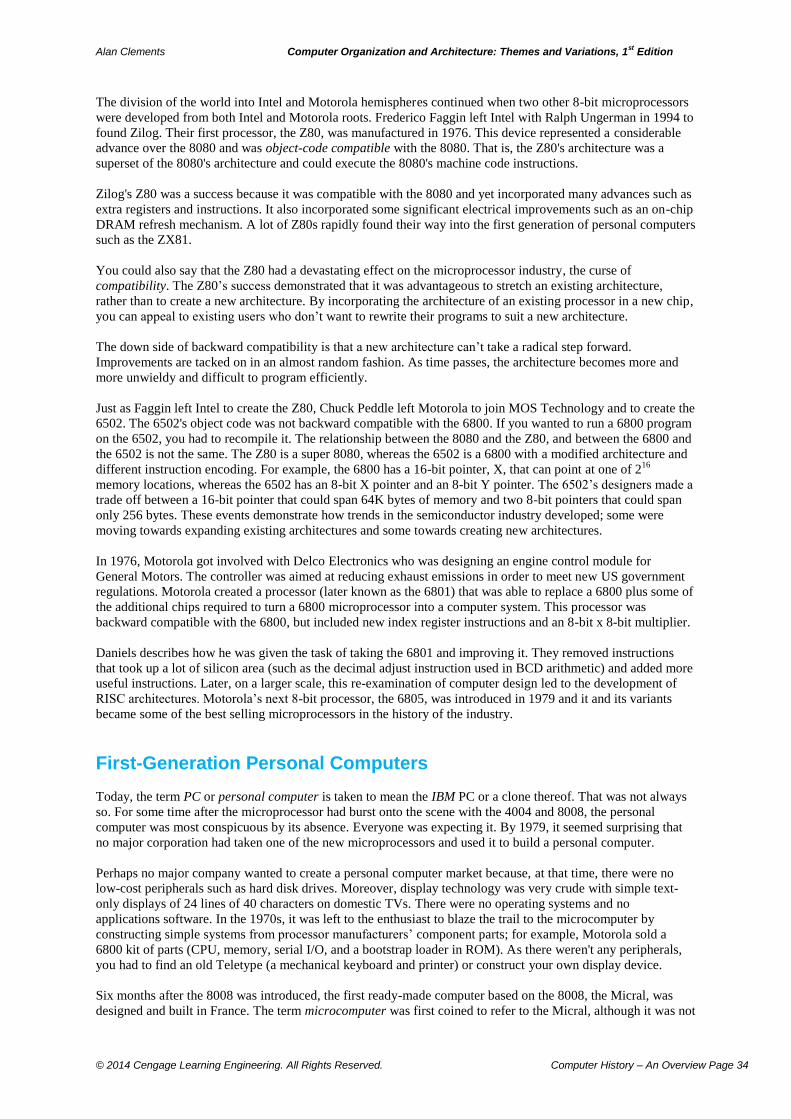
Alan Clements Computer Organization and Architecture: Themes and Variations, 1st Edition
© 2014 Cengage Learning Engineering. All Rights Reserved. Computer History – An Overview Page 34
The division of the world into Intel and Motorola hemispheres continued when two other 8-bit microprocessors
were developed from both Intel and Motorola roots. Frederico Faggin left Intel with Ralph Ungerman in 1994 to
found Zilog. Their first processor, the Z80, was manufactured in 1976. This device represented a considerable
advance over the 8080 and was object-code compatible with the 8080. That is, the Z80's architecture was a
superset of the 8080's architecture and could execute the 8080's machine code instructions.
Zilog's Z80 was a success because it was compatible with the 8080 and yet incorporated many advances such as
extra registers and instructions. It also incorporated some significant electrical improvements such as an on-chip
DRAM refresh mechanism. A lot of Z80s rapidly found their way into the first generation of personal computers
such as the ZX81.
You could also say that the Z80 had a devastating effect on the microprocessor industry, the curse of
compatibility. The Z80’s success demonstrated that it was advantageous to stretch an existing architecture,
rather than to create a new architecture. By incorporating the architecture of an existing processor in a new chip,
you can appeal to existing users who don’t want to rewrite their programs to suit a new architecture.
The down side of backward compatibility is that a new architecture can’t take a radical step forward.
Improvements are tacked on in an almost random fashion. As time passes, the architecture becomes more and
more unwieldy and difficult to program efficiently.
Just as Faggin left Intel to create the Z80, Chuck Peddle left Motorola to join MOS Technology and to create the
6502. The 6502's object code was not backward compatible with the 6800. If you wanted to run a 6800 program
on the 6502, you had to recompile it. The relationship between the 8080 and the Z80, and between the 6800 and
the 6502 is not the same. The Z80 is a super 8080, whereas the 6502 is a 6800 with a modified architecture and
different instruction encoding. For example, the 6800 has a 16-bit pointer, X, that can point at one of 216
memory locations, whereas the 6502 has an 8-bit X pointer and an 8-bit Y pointer. The 6502’s designers made a
trade off between a 16-bit pointer that could span 64K bytes of memory and two 8-bit pointers that could span
only 256 bytes. These events demonstrate how trends in the semiconductor industry developed; some were
moving towards expanding existing architectures and some towards creating new architectures.
In 1976, Motorola got involved with Delco Electronics who was designing an engine control module for
General Motors. The controller was aimed at reducing exhaust emissions in order to meet new US government
regulations. Motorola created a processor (later known as the 6801) that was able to replace a 6800 plus some of
the additional chips required to turn a 6800 microprocessor into a computer system. This processor was
backward compatible with the 6800, but included new index register instructions and an 8-bit x 8-bit multiplier.
Daniels describes how he was given the task of taking the 6801 and improving it. They removed instructions
that took up a lot of silicon area (such as the decimal adjust instruction used in BCD arithmetic) and added more
useful instructions. Later, on a larger scale, this re-examination of computer design led to the development of
RISC architectures. Motorola’s next 8-bit processor, the 6805, was introduced in 1979 and it and its variants
became some of the best selling microprocessors in the history of the industry.
First-Generation Personal Computers
Today, the term PC or personal computer is taken to mean the IBM PC or a clone thereof. That was not always
so. For some time after the microprocessor had burst onto the scene with the 4004 and 8008, the personal
computer was most conspicuous by its absence. Everyone was expecting it. By 1979, it seemed surprising that
no major corporation had taken one of the new microprocessors and used it to build a personal computer.
Perhaps no major company wanted to create a personal computer market because, at that time, there were no
low-cost peripherals such as hard disk drives. Moreover, display technology was very crude with simple text-
only displays of 24 lines of 40 characters on domestic TVs. There were no operating systems and no
applications software. In the 1970s, it was left to the enthusiast to blaze the trail to the microcomputer by
constructing simple systems from processor manufacturers’ component parts; for example, Motorola sold a
6800 kit of parts (CPU, memory, serial I/O, and a bootstrap loader in ROM). As there weren't any peripherals,
you had to find an old Teletype (a mechanical keyboard and printer) or construct your own display device.
Six months after the 8008 was introduced, the first ready-made computer based on the 8008, the Micral, was
designed and built in France. The term microcomputer was first coined to refer to the Micral, although it was not
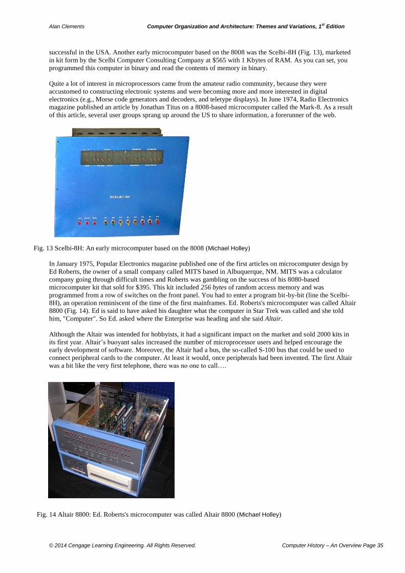
Alan Clements Computer Organization and Architecture: Themes and Variations, 1st Edition
© 2014 Cengage Learning Engineering. All Rights Reserved. Computer History – An Overview Page 35
successful in the USA. Another early microcomputer based on the 8008 was the Scelbi-8H (Fig. 13), marketed
in kit form by the Scelbi Computer Consulting Company at $565 with 1 Kbytes of RAM. As you can set, you
programmed this computer in binary and read the contents of memory in binary.
Quite a lot of interest in microprocessors came from the amateur radio community, because they were
accustomed to constructing electronic systems and were becoming more and more interested in digital
electronics (e.g., Morse code generators and decoders, and teletype displays). In June 1974, Radio Electronics
magazine published an article by Jonathan Titus on a 8008-based microcomputer called the Mark-8. As a result
of this article, several user groups sprang up around the US to share information, a forerunner of the web.
Fig. 13 Scelbi-8H: An early microcomputer based on the 8008 (Michael Holley)
In January 1975, Popular Electronics magazine published one of the first articles on microcomputer design by
Ed Roberts, the owner of a small company called MITS based in Albuquerque, NM. MITS was a calculator
company going through difficult times and Roberts was gambling on the success of his 8080-based
microcomputer kit that sold for $395. This kit included 256 bytes of random access memory and was
programmed from a row of switches on the front panel. You had to enter a program bit-by-bit (line the Scelbi-
8H), an operation reminiscent of the time of the first mainframes. Ed. Roberts's microcomputer was called Altair
8800 (Fig. 14). Ed is said to have asked his daughter what the computer in Star Trek was called and she told
him, "Computer". So Ed. asked where the Enterprise was heading and she said Altair.
Although the Altair was intended for hobbyists, it had a significant impact on the market and sold 2000 kits in
its first year. Altair’s buoyant sales increased the number of microprocessor users and helped encourage the
early development of software. Moreover, the Altair had a bus, the so-called S-100 bus that could be used to
connect peripheral cards to the computer. At least it would, once peripherals had been invented. The first Altair
was a bit like the very first telephone, there was no one to call….
Fig. 14 Altair 8800: Ed. Roberts's microcomputer was called Altair 8800 (Michael Holley)
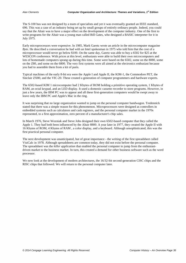
Alan Clements Computer Organization and Architecture: Themes and Variations, 1st Edition
© 2014 Cengage Learning Engineering. All Rights Reserved. Computer History – An Overview Page 36
The S-100 bus was not designed by a team of specialists and yet it was eventually granted an IEEE standard,
696. This was a case of an industry being set up by small groups of entirely ordinary people. Indeed, you could
say that the Altair was to have a major effect on the development of the computer industry. One of the first to
write programs for the Altair was a young man called Bill Gates, who designed a BASIC interpreter for it in
July 1975.
Early microprocessors were expensive. In 1985, Mark Garetz wrote an article in the microcomputer magazine
Byte. He described a conversation he had with an Intel spokesman in 1975 who told him that the cost of a
microprocessor would never go below $100. On the same day, Garetz was able to buy a 6502 for $25 at the
WESCON conference. With prices at this level, enthusiasts were able to build their own microcomputers and
lots of homemade computers sprang up during this time. Some were based on the 6502, some on the 8080, some
on the Z80, and some on the 6800. The very first systems were all aimed at the electronics enthusiast because
you had to assemble them from a kit of parts.
Typical machines of the early 8-bit era were the Apple I and Apple II, the KIM-1, the Commodore PET, the
Sinclair ZX80, and the VIC-20. These created a generation of computer programmers and hardware experts.
The 6502-based KIM 1 microcomputer had 2 Kbytes of ROM holding a primitive operating system, 1 Kbytes of
RAM, an octal keypad, and an LED display. It used a domestic cassette recorder to store programs. However, in
just a few years, the IBM PC was to appear and all these first-generation computers would be swept away to
leave only the IBM PC and Apple's Mac in the ring.
It was surprising that no large organization wanted to jump on the personal computer bandwagon. Tredennick
stated that there was a simple reason for this phenomenon. Microprocessors were designed as controllers in
embedded systems such as calculators and cash registers, and the personal computer market in the 1970s
represented, to a first approximation, zero percent of a manufacturer's chip sales.
In March 1976, Steve Wozniak and Steve Jobs designed their own 6502-based computer that they called the
Apple 1. They had both been influenced by the Altair 8800. A year later in 1977, they created the Apple II with
16 Kbytes of ROM, 4 Kbytes of RAM , a color display, and a keyboard. Although unsophisticated, this was the
first practical personal computer.
The next development was unanticipated, but of great importance - the writing of the first spreadsheet called
VisiCalc in 1978. Although spreadsheets are common today, they did not exist before the personal computer.
The spreadsheet was the killer application that enabled the personal computer to jump from the enthusiast-
driven market to the business market. In turn, this created a demand for other business software such as the word
processor.
We now look at the development of modern architectures, the 16/32-bit second-generation CISC chips and the
RISC chips that followed. We will return to the personal computer later.
Alan Clements Computer Organization and Architecture: Themes and Variations, 1st Edition
© 2014 Cengage Learning Engineering. All Rights Reserved. Computer History – An Overview Page 37
The CISC Comes of Age
Electronic engineers loved the microprocessor. Computer scientists seemed to hate it. One of my colleagues
even called it the last resort of the incompetent. Every time a new development in microprocessor architecture
excited me, another colleague said sniffily, “The Burroughs B6600 had that feature ten years ago.” From the
point of view of some computer scientists, the world seemed to be going in reverse with microprocessor features
being developed that had been around in the mainframe world for a long time. What there were missing was that
the microcomputer was being used by a very large number of people is a correspondingly large number of
applications.
The hostility shown by some computer scientists to the microprocessor was inevitable. By the mid 1970s, the
mainframe von Neumann computer had reached a high degree of sophistication with virtual memory, advanced
operating systems, 32- and 64-bit wordlengths and, in some cases, an architecture close to a high-level language.
Computer scientists regarded the new microprocessor as little more than a low-cost logic element. The 8-bit
microprocessors did not display the characteristics that computer scientists had come to expect (e.g., the ability
to manipulate complex data structures, or to implement virtual memory systems). However, electrical engineers
did not share the skepticism of their colleagues in computer science and were delighted with a device they could
Brief History of the Disk Drive A history of computing wouldn’t be complete without a mention of the disk drive that did so much to make practical computers possible. Without the ability to store large volumes of data at a low-cost per bit in a relatively small volume, computing would not have developed so rapidly. Electromagnetism, is the relationship between electricity and magnetism where a current flowing through a wire generates a magnetic field and, conversely, a moving magnetic field induces a voltage in a conductor. Hans Christian Oersted discovered that a current in a conductor created an electric field in 1819, and Michael Faraday discovered the inverse effect in 1831. Oersted’s effect can be used to magnetize materials and Faraday’s effect can be used to detect magnetization from the voltage it induces in a coil when it is moving. Electromagnetism was first used in the tape recorder to store speech and music. The first recorder that used iron wire as a storage medium was invented in the late 1890s, and the tape recorder was invented in Germany in the 1930s. The principles of the tape recorder were applied to data storage when IBM created the 305 RAMAC computer in 1956 with a 5 Mbyte disk drive. A disk drive uses a rotating platter with a read/write head that records or reads data along a circular track. The head can be stepped in or out to read one of many tracks. The amount of data stored on a disk is a function of the number of tracks and the number of bytes per inch along a track. Disk drives were very expensive initially. In the late 1960s, floppy disk drives were developed that used a removable non-rigid (floppy) plastic disc covered with a magnetic material to store data. These had a lower bit density than traditional fixed disks, but were relatively low-cost. In 1976, Shugart Associates developed the first 5¼ inch floppy disk that was to revolutionize personal computing by providing 360 KB of storage. This later became 720 KB. The adoption of the floppy disk drive by the IBM PC made the first generation of practical home computers possible. Although the 5¼ inch floppy drive gave way to 3.5 inch microfloppy drives with 1.44 MB disks in rigid plastic cases, the floppy’s days were numbered. Its capacity was very low and its access time poor. Floppy disk of all types were rendered obsolete by the much larger capacity of the optical CD drive. The hard disk drive continued to develop and by 2012 3½ inch form-factor hard drives with capacities of 3 TB were available at little more than the cost of a 3-½ inch Microdrive of three decades earlier.
Alan Clements Computer Organization and Architecture: Themes and Variations, 1st Edition
© 2014 Cengage Learning Engineering. All Rights Reserved. Computer History – An Overview Page 38
use to build powerful low-cost controllers. Electrical engineers were delighted to regain control of the device
they had invented and which they felt had been hijacked by computer scientists and their priesthood. Although a
veritable sea of computers now surrounds us, there was a time when a university's computer was located in a
special building and your only contact with it was by speaking to the operators through a glass partition.
As time passed and microprocessor technology improved, it became possible to put more and more transistors
on larger and larger chips of silicon. Microprocessors of the early 1980s were not only more powerful than their
predecessors in terms of the speed at which they could execute instructions, they were more sophisticated in
terms of the facilities they offered. For example, they supported complex addressing modes, data structures and
memory management.
The first mass-produced 16-bit microprocessor was the Texas Instruments TMS9900, a single chip version of
TI's 990 minicomputer. This device did not thrive. An interesting feature of the 9900 was its lack of on-chip user
registers. All registers were stored in memory (including the program counter, PC, and the stack pointer). A
single workspace register pointed to the set of 16 registers in RAM. Although locating registers in memory is
intrinsically slower than putting them on the chip alongside the CPU, all you have to do to change the register
set is to modify the workspace register. This feature made the TMS9900 well suited to interrupt processing and
exception handling. Although the TMS9900 was arguably superior to the 8086, it was not well supported by TI
and it never achieved the sales it deserved.
Other 16-bit processors that did not make it were the National Semiconductor Pace and the General Instruments
CP1600. The two 16-bit microprocessors that were successful were Intel's 8086 and Motorola's 68000.
Intel took the core of their 8080 microprocessor and converted it from an 8-bit into a 16-bit machine, the 8086.
In retrospect, this was a good commercial decision. However, Intel's rush to create a mass-market 16-bit
machine led to an architecture with a lot to be desired and left the world with the 640 KB memory limit on
DOS-based programs running on IBM's personal computers.
When moving from 8 bits to 16 bits, you have to deal with several issues. First, the increased instruction length
allows you to have more on-chip registers. Second, you have to decide what instructions and addressing modes
to implement. Finally, you have to decide how to expand the address space beyond 16 bits.
The 8086 had a superset of the 8080's registers; that is, all user-accessible 8080 registers were carried over to the
8086. However, the 8086 remained, essentially, a machine with a 16-bit address capable of accessing only 64K
bytes of memory. The 8080's 16-bit address bus was expanded to 20 bits by appending a 4-bit segment value;
that is, at any time the 8086 could access only one of 64 Kbytes within one of 16 segments. The total address
space was 16 × 64K = 1 Mbyte. When the 8086 was adopted by the IBM PC, 384 Kbytes were allocated to the
operating system and video display memory and the remaining 1 M – 384 K = 640 Kbytes devoted to user
programs (hence the infamous 640 Kbyte limit). We will look at the development of Intel’s 80x86 family in
more detail when we cover the IBM PC.
Motorola didn’t extend their 8-bit 6800 to create a 16-bit processor. Instead, they started again and did not
attempt to achieve either object or source code compatibility with earlier processors. By beginning with a clean
slate, Motorola created a microprocessor with an exceptionally clean architecture in 1979. We have already seen
that the 68000 had 8 general-purpose address and 8 general-purpose data registers (unlike the 8086's complex
dedicated register structure). The 68000's architecture was described as orthogonal, because an addressing mode
that could be used with one operation could also be used with a similar operation in the same class.
The 68000 was one of the first microprocessors to use microcoding to define its instruction set. The earlier
microprocessors had random logic instruction decoding and control units.
Ironically, the 68000 was not a 16-bit microprocessor, because it had a 32-bit architecture. The irony lies in the
marketing of a superior 32-bit processor as a 16-bit device in order to compete with Intel’s 16-bit 8086. The
68000 is probably the only microprocessor to have been under-hyped by its marketing department. Address and
data registers were 32 bits wide and 32-bit operations were supported. Addresses were 32-bits wide and
segmentation was not necessary. The 68000 itself had only 24 address pins and only 224
= 16 Mbytes of external
memory could be directly accessed, even though all addresses were processed as 32 bits within the chip.
At the time, the only other microprocessor in the same class was Zilog's Z8000, which had been introduced not
long after the 8086. Although nominally a 16-bit processor, the Z8000's first 8 registers could be used as sixteen

Alan Clements Computer Organization and Architecture: Themes and Variations, 1st Edition
© 2014 Cengage Learning Engineering. All Rights Reserved. Computer History – An Overview Page 39
8-bit registers, or the 16 registers could be used as eight 32-bit registers or as four 64-bit registers. The Z8000
provided a 32-bit multiplication instruction with a 64-bit product (the 68000 permitted only 16 × 16 bits to give
a 32-bit product). More importantly, the Z8000 had user and supervisor operating modes that provided the
operating system with a protection mechanism like the 68000. Due to early bugs in the Z8000's design (it had a
random logic control unit), this processor never proved successful. Zilog went on to develop a successor, the
Z80000, but by then they were too late.
Several personal computer manufacturers adopted the 68000. Apple used it in the Macintosh, and it was
incorporated in the Atari and Amiga computers. All three of these computers were regarded as technically
competent and had many very enthusiastic followers. The Macintosh was sold as a relatively high-priced black
box with the computer, software, and peripherals from a single source. This approach could not compete with
the IBM PC with an open system architecture that allowed the user to purchase hardware and software from the
supplier with the best price. The Atari and Amiga computers suffered because they had the air of the games
machine. Although the Commodore Amiga in 1985 had many of the hallmarks of a modern multimedia
machine, it was derided as a games machine because few then grasped the importance of advanced graphics and
high-quality sound. Its sophisticated operating system employed preemptive multitasking and a GUI. A few
68000-based computers were also developed for the then specialist UNIX market.
The popularity of the IBM PC and the competition between suppliers of PC clones led to ever cheaper hardware.
In turn, this led to the growth of the PC's software base.
Although the 68000 developed into the 68020, 68030, 68040, and 68060, this family ceased to be a major
contender in the personal computer world. Versions of the family were developed for the embedded processor
market, but Motorola’s 68K family played no further role in the PC world, until Apple adopted Motorola’s
PowerPC processor. The PowerPC was not a descendant of the 6800 and the 68K families.
In the early 1980s, semiconductor technology didn’t permit much more than a basic CPU on a chip. Advanced
features such as floating-pointer processors and memory management units had to be located on separate so-
called coprocessor chips that were tightly coupled to the CPU. Motorola produced both a MMU and an FFP for
its 68000 series.
In 1984, Motorola introduced the 68020 that expanded the 68000's architecture to include bit field instructions
and complex memory-indirect addressing modes. A small 256-byte instruction cache was also included on the
chip and some of the 68000's limitations preventing it from supporting true virtual memory were removed. In
many ways, you could argue that the 68020 represented the highpoint of the complex instruction set computer,
CISC, architecture development. Later members of the 68K family have concentrated on performance and have
not added to the basic architecture. Indeed, the 68060 actually dropped some of the 68020's sophisticated
instructions and emulated them in software.
Motorola's 68030, launched in 1987, was a 68020 with a larger cache and an on-chip memory management unit.
In 1989, Motorola introduced the 68040 incorporating a six-stage pipeline to improve the performance of the
underlying 68020 architecture. The 68040 also implemented a floating-point coprocessor. It is interesting that
Motorola’s 68K family not only shares architectural features of IBM’s Series/360 computers, it shares features
of their development cycle. The 68000 was developed from a basic but powerful computer into a computer with
floating point facilities, virtual memory, and on-chip cache over a decade or so.
Intel's share of the PC market ensured that it would remain heavily committed to providing a continuing upgrade
path for its old 86x family. In 1995, Motorola introduced its ColdFire line of processors. These were based on
the 68K architecture and are intended for embedded applications. Motorola eventually dropped out of the
semiconductor market and sold its processors to Freescale Semiconductor Inc. in 2004.
The RISC Challenge
A new buzzword in computer architecture arose in the 1980s, RISC. The accepted definition of RISC is reduced
instruction set computer, although the term regular instruction set computer would be more appropriate. In
practice, there is no such thing as a pure RISC processor. The term RISC simply describes a general historic
trend in computer architecture that stresses speed and simplicity over complexity. The characteristics of
processors that are described as RISC are as follows:
Alan Clements Computer Organization and Architecture: Themes and Variations, 1st Edition
© 2014 Cengage Learning Engineering. All Rights Reserved. Computer History – An Overview Page 40
Register-to-register architecture
Load and store operations are the only permitted memory accesses
Regular instruction set
Pipelined organization (instruction execution is overlapped in time)
One clock cycle per instruction goal
The origins of RISC go back to John Cocke at the IBM research center in Yorktown Heights, NY, in the mid
1970s when IBM was working on the 801 project in an attempt to improve the cost/performance ratio of
computers. IBM later used the experience gained in the 801 project when it developed its PC RT system for
small workstations in engineering and scientific applications. The RT chip had some of the characteristics of
RISC architectures, but was fabricated in relatively old MOS technology and clocked at only 6 MHz.
Consequently, the RT chip was not a commercial success, although it laid the foundations for the more
successful PowerPC.
It was the work carried out by David Paterson at the University of Berkley in the early 1980s that brought the
RISC philosophy to a wider audience. Paterson was also responsible for coining the term RISC in a paper he
wrote in 1980.
The Berkeley RISC is an interesting processor for many reasons. Although it was constructed at a university
(like many of the first mainframes, such as EDSAC), the Berkeley RISC required only a very tiny fraction of the
resources consumed by these early mainframes. Indeed, the Berkeley RISC is hardly more than an extended
graduate project. It took about a year to design and fabricate the RISC I in silicon. By 1983, the Berkeley RISC
II had been produced and that proved to be both a testing ground for RISC ideas and the start of a new industry.
The Berkeley RISC was later transformed into a commercial product, the SPARC architecture, which is one of
the few open architectures in the microprocessor world. An architecture is open if more than one manufacturer
can produce it (this is not the same as second-sourcing, where a company licenses another company to
manufacture its product).
By 1986, about ten companies were marketing processors described as RISCs.
RISC architectures were quite controversial in the 1980s, partially because the large processor manufacturers
were being told that they had been getting it wrong for the last few years and partially because a lot of the
enthusiasm for RISC architectures came out of universities rather than industry.
It is important to emphasize that at least two developments in semiconductor technology made RISC possible.
The first was the development of low-cost, high-speed memory. When memory is very expensive, complex
instructions make great sense. A complex instruction allows you to do a lot of computing for very little stored
code. Consider the 68020's instruction BFFFO ([12,A0],D1*4,8),{D4:D5},D0. This remarkably
powerful and complex instruction generates an effective address by adding 12 to the contents of pointer register
A0, reading the pointer at that address and then adding 4 times the contents of data register D1 plus 8 to the
pointer. The byte at this effective address provides the starting point for a bit field (i.e., string of bits) whose
length is in D5 and whose location is the number of bits in D4 from bit 7 of the effective address. Finally, the
processor scans the specified bit field and returns the location of the first "1" in the bit field in D0. If there's a
more complex CISC instruction than this, I'd be interested to see what it is.
This CISC instruction can do an impressive amount of computation and is specified in relatively few bits.
Carrying out the same operation with more primitive instructions would require a much larger instruction space
and hence increase system cost if memory is very expensive.
The second development that made RISC architectures possible was the increase in bus widths. An 8-bit
architecture can optimize instruction space by implementing 8-bit, 16-bit, and 24-bit instructions. Since RISC
processors have register-to-register architectures, their instructions require at least log2(op_codes) +
3log2(registers). If we assume a system with 32 registers and 265 instructions, the minimum instruction size is
log2256 + 3log232 = 8 + 15 = 23 bits.
Because RISC data processing instructions are simple, regular and don’t access memory, they can be executed
rapidly compared to CISC instructions that, for example, perform register-to-memory operations such as
ADD D1,1234 that accesses memory location 1234. Even though RSIC code is more verbose than CISC code
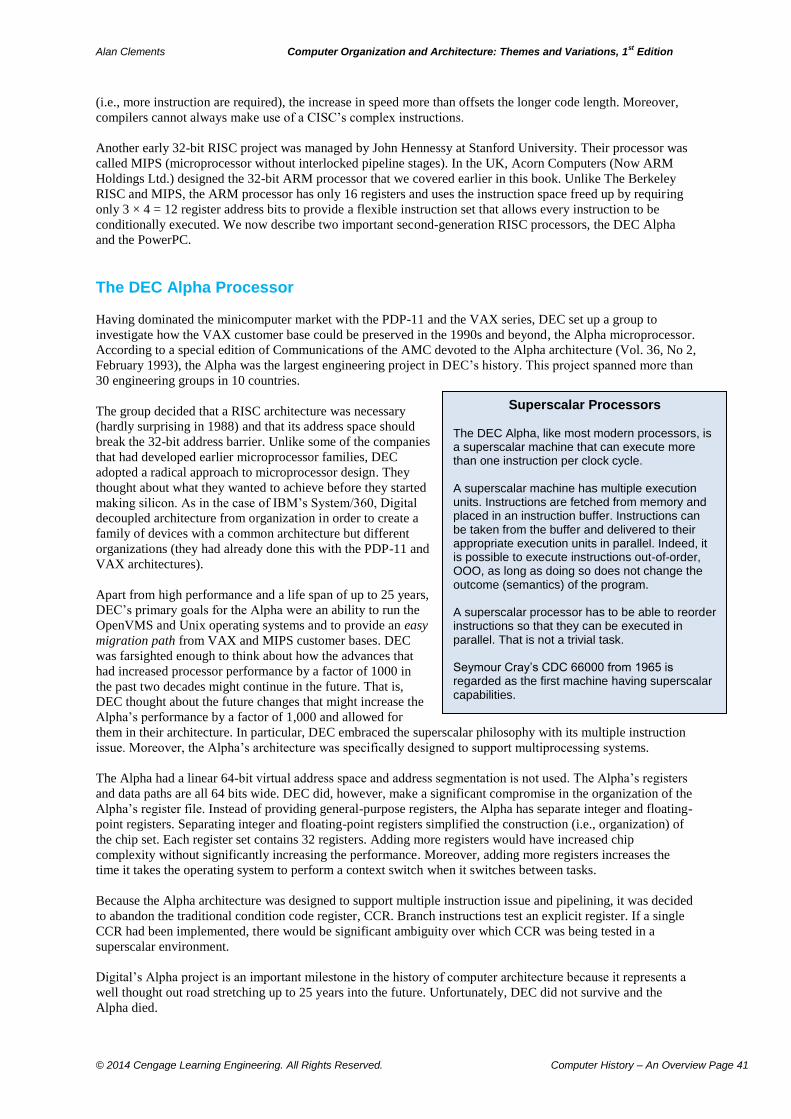
Alan Clements Computer Organization and Architecture: Themes and Variations, 1st Edition
© 2014 Cengage Learning Engineering. All Rights Reserved. Computer History – An Overview Page 41
(i.e., more instruction are required), the increase in speed more than offsets the longer code length. Moreover,
compilers cannot always make use of a CISC’s complex instructions.
Another early 32-bit RISC project was managed by John Hennessy at Stanford University. Their processor was
called MIPS (microprocessor without interlocked pipeline stages). In the UK, Acorn Computers (Now ARM
Holdings Ltd.) designed the 32-bit ARM processor that we covered earlier in this book. Unlike The Berkeley
RISC and MIPS, the ARM processor has only 16 registers and uses the instruction space freed up by requiring
only 3 × 4 = 12 register address bits to provide a flexible instruction set that allows every instruction to be
conditionally executed. We now describe two important second-generation RISC processors, the DEC Alpha
and the PowerPC.
The DEC Alpha Processor
Having dominated the minicomputer market with the PDP-11 and the VAX series, DEC set up a group to
investigate how the VAX customer base could be preserved in the 1990s and beyond, the Alpha microprocessor.
According to a special edition of Communications of the AMC devoted to the Alpha architecture (Vol. 36, No 2,
February 1993), the Alpha was the largest engineering project in DEC’s history. This project spanned more than
30 engineering groups in 10 countries.
The group decided that a RISC architecture was necessary
(hardly surprising in 1988) and that its address space should
break the 32-bit address barrier. Unlike some of the companies
that had developed earlier microprocessor families, DEC
adopted a radical approach to microprocessor design. They
thought about what they wanted to achieve before they started
making silicon. As in the case of IBM’s System/360, Digital
decoupled architecture from organization in order to create a
family of devices with a common architecture but different
organizations (they had already done this with the PDP-11 and
VAX architectures).
Apart from high performance and a life span of up to 25 years,
DEC’s primary goals for the Alpha were an ability to run the
OpenVMS and Unix operating systems and to provide an easy
migration path from VAX and MIPS customer bases. DEC
was farsighted enough to think about how the advances that
had increased processor performance by a factor of 1000 in
the past two decades might continue in the future. That is,
DEC thought about the future changes that might increase the
Alpha’s performance by a factor of 1,000 and allowed for
them in their architecture. In particular, DEC embraced the superscalar philosophy with its multiple instruction
issue. Moreover, the Alpha’s architecture was specifically designed to support multiprocessing systems.
The Alpha had a linear 64-bit virtual address space and address segmentation is not used. The Alpha’s registers
and data paths are all 64 bits wide. DEC did, however, make a significant compromise in the organization of the
Alpha’s register file. Instead of providing general-purpose registers, the Alpha has separate integer and floating-
point registers. Separating integer and floating-point registers simplified the construction (i.e., organization) of
the chip set. Each register set contains 32 registers. Adding more registers would have increased chip
complexity without significantly increasing the performance. Moreover, adding more registers increases the
time it takes the operating system to perform a context switch when it switches between tasks.
Because the Alpha architecture was designed to support multiple instruction issue and pipelining, it was decided
to abandon the traditional condition code register, CCR. Branch instructions test an explicit register. If a single
CCR had been implemented, there would be significant ambiguity over which CCR was being tested in a
superscalar environment.
Digital’s Alpha project is an important milestone in the history of computer architecture because it represents a
well thought out road stretching up to 25 years into the future. Unfortunately, DEC did not survive and the
Alpha died.
Superscalar Processors The DEC Alpha, like most modern processors, is a superscalar machine that can execute more than one instruction per clock cycle. A superscalar machine has multiple execution units. Instructions are fetched from memory and placed in an instruction buffer. Instructions can be taken from the buffer and delivered to their appropriate execution units in parallel. Indeed, it is possible to execute instructions out-of-order, OOO, as long as doing so does not change the outcome (semantics) of the program. A superscalar processor has to be able to reorder instructions so that they can be executed in parallel. That is not a trivial task. Seymour Cray’s CDC 66000 from 1965 is regarded as the first machine having superscalar capabilities.
Alan Clements Computer Organization and Architecture: Themes and Variations, 1st Edition
© 2014 Cengage Learning Engineering. All Rights Reserved. Computer History – An Overview Page 42
PowerPC
The PowerPC was the result of a joint effort between IBM, Motorola, and Apple. Essentially, IBM provided the
architecture, Motorola fabricated the chip, and Apple used it in their range of personal computers.
IBM was the first company to incorporate RISC ideas in a commercial machine, the 801 minicomputer. The 801
implemented some of the characteristics of RISC architectures and its success led IBM to develop more
powerful RISC architectures. IBM created the POWER architecture for use in their RS/6000 series
workstations. The POWER architecture had RISC features, superscalar instruction issue, but retained some
traditional CISC features such as complex bit manipulation instructions. Furthermore, POWER also provided
single-instruction multiple register transfers between the register file and memory.
A consortium of IBM, Motorola, and Apple engineers took the POWER architecture and developed it into the
PowerPC family of microprocessors. As in the case of Digital’s Alpha architecture, the PowerPC was designed
to allow for future growth and a clear distinction was made between architecture and implementation. The
POWER’s architecture was somewhat simplified and any architectural features that stood in the way of
superscalar dispatch and out-of-order executions were removed. The architecture was also extended to provide a
64-bit superset.
The first member of the PowerPC architecture was the 601, originally designed by IBM and modified by
Motorola to include some of the features of Motorola’s own RISC device, the 88110. Some of the later members
of the PowerPC family were the 603 (a low-cost, low-power processor aimed at the personal computer and
laptop market), the 604 (a high-performance version aimed at both personal computers and workstations), and
the 620 (a 64-bit version aimed at the server and workstation markets).
The PowerPC architecture never thrived in the face of Intel’s IA32 architecture. Motorola sold of its
semiconductor division, and Apple adopted Intel’s architecture. IBM continued to support the POWER
architecture for their high-end servers.
PC Revolution and the Rise of WinTel
Personal computing has been dominated by two giants, Intel and Microsoft. Just as Windows has dominated the
operating system world, Intel architectures have dominated the PC's hardware and architecture. The dominance
of the Windows operating system and the Intel family in the PC market led to the coining of the term WinTel to
describe the symbiotic relationship between the Microsoft Corporation and Intel.
The relationship between Microsoft and Intel is not entirely cosy. Although Intel's chips and Microsoft's
operating system form the foundations of the personal computer, each of these two organizations views the
world from a different perspective. Microsoft is happy to see other semiconductor manufacturers produce clones
of Intel processors. If chip prices are driven down by competition, people can afford to pay more for Microsoft's
software. Similarly, if the freely available Linux operating system becomes more widely available, Intel can sell
more chips for Linux boxes. Linux is an open-source operating system, functionally equivalent to Unix, named
after Linus Torvalds who created the first version of its kernel (core) while a student at the University of
Helsinki in 1991.
IBM PCs – The Background
The success of the first serious personal computer, the 6502-based Apple II introduced in 1977, demonstrated
that there was a potential mass market for personal computers. The development of microprocessor architectures
since 1981 has been affected as much by commercial considerations as by improvements in technology because
of the inexorable rise of the IBM PC. A cynical observer might suggest that the PC owes an immense debt of
gratitude to Apple, for failing to capitalize on its 68000-based Macintosh that so many people once regarded as
superior to the IBM PC.
Apple's failure to displace the IBM PC demonstrates that those in the semiconductor industry must realize that
commercial factors are every bit as important as architectural excellence and performance. IBM adopted open
standards, and, by making the IBM PC non-proprietary, anyone could build a copy, or clone, of the PC.
Alan Clements Computer Organization and Architecture: Themes and Variations, 1st Edition
© 2014 Cengage Learning Engineering. All Rights Reserved. Computer History – An Overview Page 43
Hundreds of manufacturers started producing parts of PCs and an entire industry sprang up. You could buy a
basic system from one place, a hard disk from another, and a graphics card from yet another supplier. Publishing
standards for the PC's bus, enables anyone to create a peripheral for the PC. What IBM lost in the form of
increased competition, they more than made up for in the rapidly expanding market. Finally, IBM’s open
standard provided an incentive for software writers to generate software for the rapidly expanding PC market.
Apple favored a very different approach. They marketed the computer. And the operating system. And the
peripherals. Apple refused to publish detailed hardware specifications or to license their BIOS and operating
system. Apple may well have had the better processor and an operating system that was regarded as more user
friendly. In particular, non-computer specialists loved the Apple because they found it so easy to use in contrast
with the PC. Even though you could buy peripherals for the PC from many sources, getting, say, a video card to
work with your operating system could sometimes prove very difficult. Of course, this applies largely to the
past. Today, more advanced operating systems, USB, and WiFi make is remarkably easy to install new
hardware and software in a PC.
As time passed, the sheer volume of PCs and their interfaces (plus the software base) pushed PC prices down
and down. The Apple was perceived as overpriced. Even though Apple adopted the PowerPC, it was too late
and Apple's role in the personal computer world was marginalized. By the mid 1990s, it was possible to joke,
"Question: What do you get if you merge Apple with IBM? Answer: IBM". Unlike many other computer
companies, Apple did not fade away. They developed stylish mobile devices, beginning with MP3 players, then
cell phones that incorporated many of the functions of a personal computer, and then tablet computers that
included everything from a camera to a satnav system to a cellphone to an electronic book.
Tredennick points out that the fundamental problem facing anyone who wishes to break into the PC field is
amortization. A manufacturer has to recover its development costs over its future sales. Intel can spread the cost
of a processor over, say, millions of units. In other words, the amortization cost of each processor is just a few
dollars and is well below its manufacturing costs. On the other hand, a competitor attempting to break into the
market will have to amortize development costs over a much smaller number of processors.
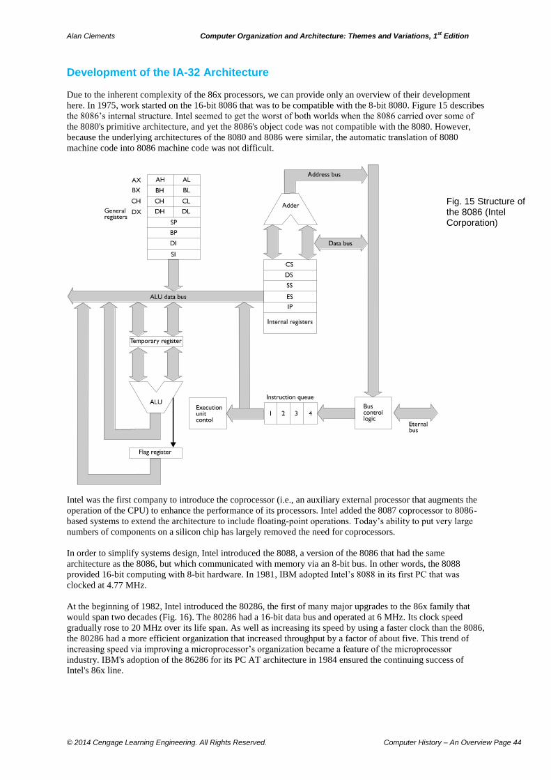
Alan Clements Computer Organization and Architecture: Themes and Variations, 1st Edition
© 2014 Cengage Learning Engineering. All Rights Reserved. Computer History – An Overview Page 44
Development of the IA-32 Architecture
Due to the inherent complexity of the 86x processors, we can provide only an overview of their development
here. In 1975, work started on the 16-bit 8086 that was to be compatible with the 8-bit 8080. Figure 15 describes
the 8086’s internal structure. Intel seemed to get the worst of both worlds when the 8086 carried over some of
the 8080's primitive architecture, and yet the 8086's object code was not compatible with the 8080. However,
because the underlying architectures of the 8080 and 8086 were similar, the automatic translation of 8080
machine code into 8086 machine code was not difficult.
Fig. 15 Structure of the 8086 (Intel Corporation)
Intel was the first company to introduce the coprocessor (i.e., an auxiliary external processor that augments the
operation of the CPU) to enhance the performance of its processors. Intel added the 8087 coprocessor to 8086-
based systems to extend the architecture to include floating-point operations. Today’s ability to put very large
numbers of components on a silicon chip has largely removed the need for coprocessors.
In order to simplify systems design, Intel introduced the 8088, a version of the 8086 that had the same
architecture as the 8086, but which communicated with memory via an 8-bit bus. In other words, the 8088
provided 16-bit computing with 8-bit hardware. In 1981, IBM adopted Intel’s 8088 in its first PC that was
clocked at 4.77 MHz.
At the beginning of 1982, Intel introduced the 80286, the first of many major upgrades to the 86x family that
would span two decades (Fig. 16). The 80286 had a 16-bit data bus and operated at 6 MHz. Its clock speed
gradually rose to 20 MHz over its life span. As well as increasing its speed by using a faster clock than the 8086,
the 80286 had a more efficient organization that increased throughput by a factor of about five. This trend of
increasing speed via improving a microprocessor’s organization became a feature of the microprocessor
industry. IBM's adoption of the 86286 for its PC AT architecture in 1984 ensured the continuing success of
Intel's 86x line.
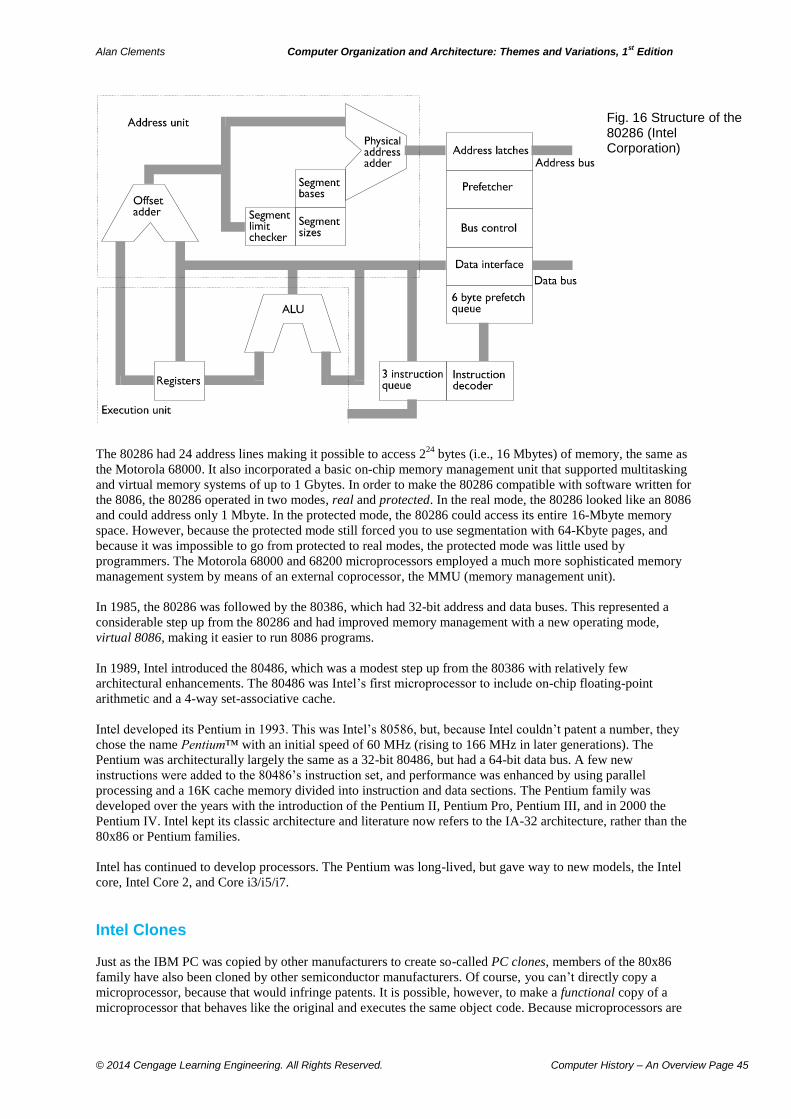
Alan Clements Computer Organization and Architecture: Themes and Variations, 1st Edition
© 2014 Cengage Learning Engineering. All Rights Reserved. Computer History – An Overview Page 45
Fig. 16 Structure of the 80286 (Intel Corporation)
The 80286 had 24 address lines making it possible to access 224
bytes (i.e., 16 Mbytes) of memory, the same as
the Motorola 68000. It also incorporated a basic on-chip memory management unit that supported multitasking
and virtual memory systems of up to 1 Gbytes. In order to make the 80286 compatible with software written for
the 8086, the 80286 operated in two modes, real and protected. In the real mode, the 80286 looked like an 8086
and could address only 1 Mbyte. In the protected mode, the 80286 could access its entire 16-Mbyte memory
space. However, because the protected mode still forced you to use segmentation with 64-Kbyte pages, and
because it was impossible to go from protected to real modes, the protected mode was little used by
programmers. The Motorola 68000 and 68200 microprocessors employed a much more sophisticated memory
management system by means of an external coprocessor, the MMU (memory management unit).
In 1985, the 80286 was followed by the 80386, which had 32-bit address and data buses. This represented a
considerable step up from the 80286 and had improved memory management with a new operating mode,
virtual 8086, making it easier to run 8086 programs.
In 1989, Intel introduced the 80486, which was a modest step up from the 80386 with relatively few
architectural enhancements. The 80486 was Intel’s first microprocessor to include on-chip floating-point
arithmetic and a 4-way set-associative cache.
Intel developed its Pentium in 1993. This was Intel’s 80586, but, because Intel couldn’t patent a number, they
chose the name Pentium™ with an initial speed of 60 MHz (rising to 166 MHz in later generations). The
Pentium was architecturally largely the same as a 32-bit 80486, but had a 64-bit data bus. A few new
instructions were added to the 80486’s instruction set, and performance was enhanced by using parallel
processing and a 16K cache memory divided into instruction and data sections. The Pentium family was
developed over the years with the introduction of the Pentium II, Pentium Pro, Pentium III, and in 2000 the
Pentium IV. Intel kept its classic architecture and literature now refers to the IA-32 architecture, rather than the
80x86 or Pentium families.
Intel has continued to develop processors. The Pentium was long-lived, but gave way to new models, the Intel
core, Intel Core 2, and Core i3/i5/i7.
Intel Clones
Just as the IBM PC was copied by other manufacturers to create so-called PC clones, members of the 80x86
family have also been cloned by other semiconductor manufacturers. Of course, you can’t directly copy a
microprocessor, because that would infringe patents. It is possible, however, to make a functional copy of a
microprocessor that behaves like the original and executes the same object code. Because microprocessors are
Alan Clements Computer Organization and Architecture: Themes and Variations, 1st Edition
© 2014 Cengage Learning Engineering. All Rights Reserved. Computer History – An Overview Page 46
so complex, it is impossible to verify that an 80x86
or Pentium clone is exactly functionally equivalent to
an actual 80x86/Pentium. For this reason, some users
have been reluctant to use 80x86 clones.
The first Intel clone was the Nx586 produced by
NextGen ,which was later taken over by AMD. This
chip provided a similar level of performance to early
Pentiums, running at about 90 MHz, but was sold at
a considerably lower price. The Nx586 had several
modern architectural features such as superscalar
execution with two integer execution units,
pipelining, branch prediction logic, and separate data
and instruction caches. The Nx586 could execute up
to two instructions per cycle.
The Nx586 didn’t attempt to execute Intel’s
instruction set directly. Instead, it translated IA32
instructions into a simpler form and executed those
instructions.
Other clones were produced by AMD and Cyrix.
AMD’s K5 took a similar approach to NexGen by
translating Intel’s variable-length instructions into
fixed-length RISC instructions before executing
them. AMD’s next processor, the K6, built on
NexGen’s experience by including two instruction
pipelines fed by four instruction decoders.
By early 1999, some of the clone manufacturers were attempting to improve on Intel’s processors rather than
just creating lower cost, functionally equivalent copies. Indeed AMD claimed that its K7 or Athlon architecture
was better than the corresponding Pentium III; for example, the Athlon provided 3DNow! technology that
boosted graphics performance, a level 1 cache four times larger than that in Intel’s then competing Pentium III,
and a system bus that was 200% faster than Intel’s (note that AMD’s processors required a different mother
board to Intel’s chips).
In 1995, Transmeta was set up specifically to market a processor called Crusoe that would directly compete with
Intel’s Pentium family, particularly in the low-power laptop market. Crusoe’s native architecture was nothing
like the IA32 family that it emulated. It used a very long instruction word format to execute instructions in
parallel. When IA32 (i.e., x68) instructions were read from memory, they were dynamically translated into
Crusoe’s own code in a process that Transmeta called code morphing). The translated code was saved in a cache
memory and the source code didn’t need to be translated the next time it was executed. Because Crusoe’s
architecture was more efficient than the IA32 family, the first version of Crusoe had about one-quarter the
number of transistors of an equivalent Intel processors. Consequently, Transmeta were able to claim that their
device was both faster and less power-hungry than Intel’s chips. In fact, Transmeta’s processors did not live up
to their claims and the company failed.
MS-DOS and Windows
Although hardware and software inhibit different universes, there are points of contact; for example, it is
difficult to create a new architecture in the absence of software, and computer designers create instruction stets
to execute real software. Users interact with operating systems in one of two ways: via a command languages
like UNIX and MS-DOS, or via a graphical user interface like Windows. The user interface is, of course, only a
means of communication between the human and the operating system; the underlying operating system that
manages files and switches between tasks is not directly affected by the user interface. Here we take a brief look
at two user interfaces: the command-line driven MS-DOS, and the Windows graphical user interface.
Clones and Patents You can’t patent or copyright a computer’s instruction set or a language. However, chip manufacturers have attempted to use patent law to limit what other companies can do. Although you can’t patent an instruction, you can patent any designs and methods necessary to implement the instruction. If you manage to do this, then a manufacturer would not be able to bring out a clone using your instruction set because they would automatically infringe your copyright if they attempted to implement the protected instruction. An interesting example is provided by Jonah Probel who worked for Lexra, a microprocessor company. Lexra built a RISC processor with the same instruction set as the MIPS. However, four MIPS instructions, lwl, lwr, swl, and swr that perform unaligned memory store and loads are protected by US patent 4,814,976. These instructions allow you to execute a memory access across word boundaries; that is, one bytes of a word might be at one word address and the second byte at the next word address.
Lexra was aware of the patent and chose not to implement these instructions in hardware, but to trap (i.e., detect) them and emulate them in software using other instructions. However, MIPS Technologies contested even this action, although the code to implement unaligned accesses was in common use.
Alan Clements Computer Organization and Architecture: Themes and Variations, 1st Edition
© 2014 Cengage Learning Engineering. All Rights Reserved. Computer History – An Overview Page 47
Operating systems have been around for a long
time and their history is as fascinating as that of
the processor architectures themselves. In the early
days of the computer when all machines were
mainframes, manufacturers designed operating
systems to run on their own computers.
One of the first operating systems that could be
used on a variety of different computers was
UNIX, which was designed by Ken Thompson and
Dennis Richie at Bell Labs. UNIX was written in
C; a systems programming language designed by
Richie. Originally intended to run on DEC’s
primitive PDP-7 minicomputer, UNIX was later
rewritten for the popular PDP-11. This proved to
be an important move, because, in the 1970s,
many university computer science departments used PDP-11s. Bell Labs licensed UNIX for a nominal fee and it
rapidly became the standard operating system in the academic world.
UNIX is a powerful and popular operating system because it operates in a consistent and elegant way. When a
user logs in to a UNIX system, a program called the shell interprets the user’s commands. These commands take
a little getting used to, because they are heavily abbreviated and the abbreviations are not always what you
might expect. UNIX’s immense popularity in the academic world has influenced the thinking of a generation of
programmers and systems designers.
The first command-line operating system designed to run on IBM’s PC was MS-DOS. In 1980, IBM
commissioned Bill Gates to produce an operating system for their new PC. IBM was aware of Bill Gates
because he had written a version of the language BASIC for the Intel 8080-based Altair personal computer.
Because IBM’s original PC had only 64K bytes of RAM and no hard disk, a powerful operating system like
UNIX could not be supported. Gates didn’t have time to develop an entirely new operating system, so his
company, Microsoft, bought an operating system called 85-DOS which was modified and renamed MS-DOS
(Microsoft Disk Operating System).
Version 1.0 of MS-DOS, released in 1981, occupied 12K bytes of memory and supported only a 160 Kbyte 5¼
in diskette. MS-DOS performed all input and output transactions by calling routines in a read-only memory
within the PC. These I/O routines are known as the BIOS (basic input/output system). MS-DOS 1.0 also
included a command processor, command.com, like UNIX’s shell.
Over the years, Microsoft refined MS-DOS to take advantage of the improved hardware of later generations of
PCs. MS-DOS 1.0 begat version 1.1, which begat version 2.0, and so on. After much begetting, which made Bill
Gates one of the richest men in the World, MS-DOS reached version 6.2 in 1994. New versions of MS-DOS
were eagerly awaited, and many PC users purchase the updates as soon as they are released. With so many
versions of MS-DOS sold in such a short time, you could be forgiven for making the comment “You don’t buy
MS-DOS. You rent it”.
MS-DOS shares many of the features of UNIX, but lacks UNIX’s consistency. More importantly, the pressure
to maintain backward compatibility with older versions of PC hardware and software meant that MS-DOS could
not handle programs larger than 640 Kbytes. MS-DOS was designed for the 8086 microprocessor with only
1 Mbyte of address space. Unlike UNIX, MS-DOS was not designed as a timesharing system and has no logon
procedure. In other words, MS-DOS has no security mechanism and the user can do anything he or she wants.
UNIX has a superuser protected by a password who has special privileges. The superuser is able to configure
and maintain the operating system.
An MS-DOS file name was restricted to eight characters (UNIX file names can be up to 255 characters). UNIX
and MS-DOS allowed the file type to be described by an extension after the filename; for example, the MS-DOS
file test.exe indicates a file called test that is in the form of executable code. Neither UNIX nor MS-DOS
enforced the way in which file extensions are used. You could give a file any extension you want.
MS-DOS could be configured for the specific system on which it is to run. When MS-DOS was first loaded into
memory, two files called CONFIG.SYS and AUTOEXEC.BAT were automatically executed. These files set up
UNIX Considered Unlovely UNIX is a very powerful and flexible, interactive, timesharing operating system that was designed by programmers for programmers. What does that mean? If I said that laws are written for lawyers, I think that a picture might be forming in your mind. UNIX is a user-friendly operating system like a brick is an aerodynamically efficient structure. However, UNIX is probably the most widely used operating system in many universities. Andrew Tanenbaum, the well-known computer scientist saw things differently and said: “While this kind of user interface [a user-friendly system] may be suitable for novices, it tends to annoy skilled programmers. What they want is a servant, not a nanny.”
Alan Clements Computer Organization and Architecture: Themes and Variations, 1st Edition
© 2014 Cengage Learning Engineering. All Rights Reserved. Computer History – An Overview Page 48
an environment to suit the structure of the computer and told the operating system where to find device drivers
for the video display, mouse, printer, sound card, and so on. The MS-DOS’s configuration files allowed the
system to be tailored to suit the actual software and hardware environment.
Some believe that one of the most important factors in encouraging the expansion of computers into non-
traditional environments was the
development of intuitive, user-friendly
interfaces. On the other hand, every time
you installed a new package, there was a
good chance that it would modify the
configuration files. After a time, the
configuration files became very difficult to
understand. Even worse, when you deleted
an application, the changes it made to the
configuration file were left behind.
Like UNIX, MS-DOS is well suited to
programmers. The need to make computers
accessible to all those who want to employ
them as a tool, forced the development of
graphical user interfaces, GUIs, like
Windows. A graphical interface lets you
access operating system functions and run
applications programs without ever reading
the user’s manual. Some programmers
didn’t like the GUI environment because
they felt that the traditional command
language was much more efficient and
concise. Graphical user interfaces are now
standard on devices such as MP3 players,
digital cameras, iPads, and smart cell
phones. Indeed, many people using these
devices don’t even realize that they are
using an operating system.
Before we discuss the history of Windows,
we have to say something about Linux.
Essentially, Linux is a public-domain clone
of AT&T’s UNIX. In 1987, Andrew
Tanenbaum designed Minix, an open-
source operating system, as a tool for study
and modification in operating system
courses. Linus Torvalds, a computer
science student in Finland, was inspired by Minix to create his own operation system, Linux. Version 0.01 of
Linux was released in 1991. Torvalds’ operating system has steadily grown in popularity and, although in the
public domain, numerous companies sell versions of it with add-ons and tools. The amount of software available
to those running Linux has steadily increased.
Apple’s operating system, OS-X, is based on UNIX with a graphical front end.
Windows
Many of today’s computers will be unaware of Microsoft’s early history and MS-DOS; all they will be aware of
is Microsoft’s user-friendly, graphical operating system known as Windows. Graphical interfaces have a long
history. The credit for the development of graphical user interfaces is usually given to Xerox for their work at
Xerox PARC at the Palo Alto Research Center in the late 1970s. They developed the Alto and the Xerox Star,
the first GUI-based computers. Xerox’s computers were not commercially successful and the first significant
computer to use a GUI interface was Apple’s Lisa and its more famous successor the Apple Macintosh.
The Serial Interface—Key to Personal Computing A computer needs peripherals such as a keyboard, mouse, display, printer, scanner, and an interface to the external world. Without these, the computer is little more than a calculator. Interfaces to the mouse, keyboard, and display were initially provided directly; that is, you plugged these peripherals into the computer. Anything else was a different story. PCs were provides with an asynchronous serial data link conforming to the RS-232 standard. This standard was introduced in 1962, long before the microprocessor age, and was intended to interface data communications equipment, CDE, to data terminal equipment, DCE operating over a relatively slow serial data link. Version of the standard, RS232C, that was most frequently used by PCs dates back to 1969. RSC32-C links connected personal computers to printers and modems (telephone network interfaces). In short, this interface was a mess. It was never intended for PC use. It belonged to a pre-microprocessor age, was dreadfully slow, and had facilities and functions that were intended for dial-up telephone networks operating at, typically, 9,600 bits/s. Moreover, you often had to configure both its hardware interface and its software for each application. In 1994 a group of seven companies including Microsoft devised a serial interface link using a lightweight 4-core shielded cable with dedicated plugs at both ends that could operate at up to 12 Mbits/s. This was the universal serial bus, USB, that was to revolutionize personal computing. Not only was USB faster than RS232C, it supported a multi-peripheral topology (RS232C was strictly point-to-point) and USB devices used software or firmware to negotiate for the serial bus and to control data exchanges. USB brought plug and play to computers where all you had to do to interface a new peripheral was to plug it in. By 2012 the USB standard had been revised several times and USB 3.0 was current with a maximum theoretical data rate of 5 Gbits/s. The practical maximum data rate was considerably less, but still sufficient for most multimedia applications. I have always argued that the two real stars of the computer world are the USB interface and flash memory.
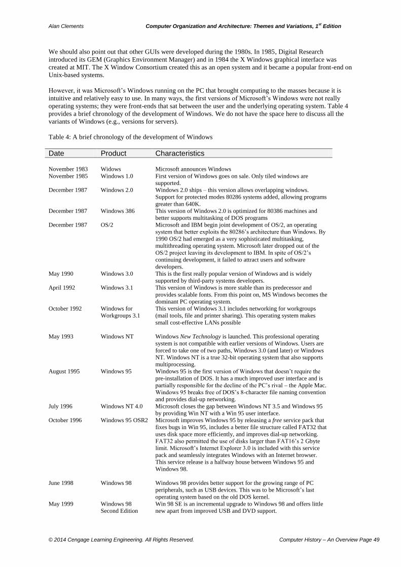
Alan Clements Computer Organization and Architecture: Themes and Variations, 1st Edition
© 2014 Cengage Learning Engineering. All Rights Reserved. Computer History – An Overview Page 49
We should also point out that other GUIs were developed during the 1980s. In 1985, Digital Research
introduced its GEM (Graphics Environment Manager) and in 1984 the X Windows graphical interface was
created at MIT. The X Window Consortium created this as an open system and it became a popular front-end on
Unix-based systems.
However, it was Microsoft’s Windows running on the PC that brought computing to the masses because it is
intuitive and relatively easy to use. In many ways, the first versions of Microsoft’s Windows were not really
operating systems; they were front-ends that sat between the user and the underlying operating system. Table 4
provides a brief chronology of the development of Windows. We do not have the space here to discuss all the
variants of Windows (e.g., versions for servers).
Table 4: A brief chronology of the development of Windows
Date Product Characteristics November 1983 Widows Microsoft announces Windows
November 1985 Windows 1.0 First version of Windows goes on sale. Only tiled windows are
supported.
December 1987 Windows 2.0 Windows 2.0 ships – this version allows overlapping windows.
Support for protected modes 80286 systems added, allowing programs
greater than 640K.
December 1987 Windows 386 This version of Windows 2.0 is optimized for 80386 machines and
better supports multitasking of DOS programs
December 1987 OS/2 Microsoft and IBM begin joint development of OS/2, an operating
system that better exploits the 80286’s architecture than Windows. By
1990 OS/2 had emerged as a very sophisticated multitasking,
multithreading operating system. Microsoft later dropped out of the
OS/2 project leaving its development to IBM. In spite of OS/2’s
continuing development, it failed to attract users and software
developers.
May 1990 Windows 3.0 This is the first really popular version of Windows and is widely
supported by third-party systems developers.
April 1992 Windows 3.1 This version of Windows is more stable than its predecessor and
provides scalable fonts. From this point on, MS Windows becomes the
dominant PC operating system.
October 1992 Windows for
Workgroups 3.1
This version of Windows 3.1 includes networking for workgroups
(mail tools, file and printer sharing). This operating system makes
small cost-effective LANs possible
May 1993 Windows NT Windows New Technology is launched. This professional operating
system is not compatible with earlier versions of Windows. Users are
forced to take one of two paths, Windows 3.0 (and later) or Windows
NT. Windows NT is a true 32-bit operating system that also supports
multiprocessing.
August 1995 Windows 95 Windows 95 is the first version of Windows that doesn’t require the
pre-installation of DOS. It has a much improved user interface and is
partially responsible for the decline of the PC’s rival – the Apple Mac.
Windows 95 breaks free of DOS’s 8-character file naming convention
and provides dial-up networking.
July 1996 Windows NT 4.0 Microsoft closes the gap between Windows NT 3.5 and Windows 95
by providing Win NT with a Win 95 user interface.
October 1996 Windows 95 OSR2 Microsoft improves Windows 95 by releasing a free service pack that
fixes bugs in Win 95, includes a better file structure called FAT32 that
uses disk space more efficiently, and improves dial-up networking.
FAT32 also permitted the use of disks larger than FAT16’s 2 Gbyte
limit. Microsoft’s Internet Explorer 3.0 is included with this service
pack and seamlessly integrates Windows with an Internet browser.
This service release is a halfway house between Windows 95 and
Windows 98.
June 1998 Windows 98 Windows 98 provides better support for the growing range of PC
peripherals, such as USB devices. This was to be Microsoft’s last
operating system based on the old DOS kernel.
May 1999 Windows 98
Second Edition
Win 98 SE is an incremental upgrade to Windows 98 and offers little
new apart from improved USB and DVD support.
Alan Clements Computer Organization and Architecture: Themes and Variations, 1st Edition
© 2014 Cengage Learning Engineering. All Rights Reserved. Computer History – An Overview Page 50
February 2000 Windows 2000 Windows 2K is really an update to Windows NT 4.0 rather than
Windows 98. However, Windows 2000 was priced at the domestic
consumer. This is a full 32-bit operating system with multiprocessing
capabilities, and with Win NT 4.0’s NTFS filing system that increases
security by protecting system files. Its initial uptake was weak because
it required new device drivers and many found that their peripherals
would not work with Windows 2K. Microsoft released both personal
and professional (i.e., server) versions of Win 2K.
September 2000 Windows ME Windows Millennium Edition was aimed at the home user who wished
to upgrade from Windows 98 SE without going to Windows 2K.
Windows ME includes strong support for the growth of multimedia
applications such as digital video and sound processing. Windows ME
still included some 16-bit code from the Win 98 era and does not
support multiprocessing.
2001 Windows XP Windows XP represented a merging of Widows NT2000 and the series
of Windows 95, 96, and ME. Microsoft developed a range of XP
operating systems, each targeted on a different market sector: Home
Edition, Professional, Media Center Edition, Tablet Edition,
Embedded, and a 64-bit edition.
November 2006 Windows Vista Vista was an improved version of XP that had a higher level of
security (i.e., greater tolerance to malware). Life XP, Vista was sold in
a range of different editions.
July 2009 Windows 7 Windows 7 was also available in multiple editions and represented
another incremental step in the Windows development cycle. Most PC
systems sold with Windows pre-installed used Windows 7 64-bit.
2012 Windows 8
Windows 8 appeared at a time when Microsoft was coming under
threat from new forms of user friendly operating systems that had been
appearing on tablet computers and in mobile phones (e.g., Android,
BlackBerry and Symbian). These operating systems are App
(application) driven. Windows 8 ventures into the mobile phone,
tablet, and touch screen territory while attempting to retain traditional
professional users.
© Cengage Learning 2014
The Phenomenon of Mass Computing and the Rise of the Internet By the late 1990s, the PC was everywhere (at least in developed countries). Manufacturers have to sell more and
more of their products in order to expand. PCs had to be sold into markets that were hitherto untouched; that is,
beyond the semiprofessional user and the games enthusiast.
Two important applications have driven the personal computer expansion, the Internet and digital multimedia.
The Internet provides interconnectivity on a scale hitherto unimagined. Many of the classic science fiction
writers of the 1940s and 1950s (such as Isaac Asimov) predicted the growth of the computer and the rise of
robots, but they never imagined the Internet and the ability of anyone with a computer to access the vast
unstructured source of information that now comprises the Internet.
Similarly, the digital revolution has extended into digital media—sound and vision. The tape-based personal
stereo system was first displaced by the minidisk and then the solid state memory-based MP3 players. The DVD
with its ability to store an entire movie on a single disk first became available in 1996 and by 1998 over one
million DVD players had been sold in the USA. The digital movie camera that once belonged to the world of the
professional filmmaker first became available to the wealthy enthusiast and now anyone with a modest income
can afford a high-resolution camcorder.
All these applications have had a profound effect on the computer world. Digital video requires truly vast
amounts of storage. Within a four- or five-year span, low-cost hard disk capacities grew from about 1 Gbytes to
60 Gbytes or more. The DVD uses highly sophisticated signal processing techniques that require very high-
performance hardware to process the signals in real-time. The MP3 player requires a high-speed data link to
download music from the Internet. By 2012, the capacity of hard disk drives had risen to 3 TBytes and Blue-ray
read/write optical disks were widely available.
Alan Clements Computer Organization and Architecture: Themes and Variations, 1st Edition
© 2014 Cengage Learning Engineering. All Rights Reserved. Computer History – An Overview Page 51
We can’t neglect the effect of computer games on computer technology. The demand for increasing reality in
video games and real-time image processing has spurred the development of special-purpose video subsystems.
Video processing requires the ability to render images, which means drawing vast numbers of polygons on the
screen and filling them with a uniform color. The more polygons used to compose an image, the more accurate
the rendition. This has led to the development of graphics engines with hundreds of independent processors
(cores) on the same chip.
The effect of the multimedia revolution has led to the commoditization of the PC, which is now just another
consumer item like a television or a stereo player. Equally, the growth of multimedia has forced the
development of higher speed processors, low-cost high-density memory systems, multimedia aware operating
systems, data communications, and new processor architectures.
It would be wrong to give the impression that the PC and the Internet are the only applications of the computer.
The largest user of the microprocessor is probably the automobile with tens of microprocessors embedded in
each machine (e.g., in radios to tune the receiver and operate the display, in CDs to perform motor control,
audio decoding, in engine control, in automatic braking systems, in lighting, door and window controls, and so
on). Similarly, one or more microprocessors are embedded in every cell phone where the system had to be
optimized for both performance and power consumption.
The Internet Revolution
No history of computers can ignore the effect of the Internet on computer development. Although the Internet is
not directly related to computer architecture, the Internet has had a major effect on the way in which the
computer industry developed because users want computers that can access the Internet easily and run video-
and sound-intensive applications.
It is impossible to do justice to the development of the Internet and the World Wide Web in a few paragraphs
and we will, therefore, describe only some of the highlights of its development.
Just as the computer itself was the result of many independent developments (the need for automated
calculation, the theoretical development of computer science, the enabling technologies of communications and
electronics, the keyboard, and data processing industries), the Internet was also the fruit of multiple
developments.
The principal ingredients of the Internet are communications, protocols, and hypertext. Communications
systems have been developed throughout human history, as we have already pointed out when discussing the
enabling technology behind the computer. The USA’s Department of Defense created a scientific organization,
Advanced Research Projects Agency (ARPA), in 1958 at the height of the Cold War. ARPA had some of the
characteristics of the Manhattan project that had preceded it during World War II; for example, large group of
talented scientists were assembled to work on a project of national importance. From its early days, ARPA
concentrated on computer technology and communications systems. Moreover, ARPA was moved into the
academic area, which meant that it had a rather different ethos to that of the commercial world. Academics tend
to cooperate and share information.
One of the reasons that ARPA concentrated on networking was the fear that a future war involving nuclear
weapons would begin with an attack on communications centers, limiting the capacity to respond in a
coordinated manner. By networking computers and ensuring that a message can take many paths through the
network to get from its source to its destination, the network can be made robust and able to cope with the loss
of some of its links or switching centers.
In 1969, ARPA began to construct a test bed for networking, a system that linked four nodes: University of
California at Los Angeles, SRI (in Stanford), University of California at Santa Barbara, and University of Utah.
Data was sent in the form of individual packets or frames rather than as complete end-to-end messages. In 1972,
ARPA was renamed DARPA (Defense Advanced Research Projects Agency).
In 1973, the transmission control/Internet protocol, TCP/IP, was developed at Stanford; this is the set of rules
that govern the routing of a packet from node to node through a computer network. Another important step on
the way to the Internet was Robert Metcalfe’s development of the Ethernet that enabled computers to
Alan Clements Computer Organization and Architecture: Themes and Variations, 1st Edition
© 2014 Cengage Learning Engineering. All Rights Reserved. Computer History – An Overview Page 52
communicate with each other over a local area network based using a simple low-cost coaxial cable. The
Ethernet made it possible to link computers in a university together, and the ARPANET allowed the universities
to be linked together. Ethernet was based on techniques developed during the construction of the University of
Hawaii’s radio-based packet-switching ALOHAnet, another ARPA-funded project.
In 1979, Steve Bellovin and others at the
University of North Carolina constructed
a news group network called USENET
based on a UUCP (Unix-to-Unix Copy
protocol) developed by AT&T’s Bell
Labs. At this point we have a network of
computers in academic institutions that
can be freely used by academics to
exchange information.
Up to 1983, ARPANET a user had to
use a numeric Internet Protocol, IP,
address to access another user. In 1983,
the University of Wisconsin created the
Domain Name System (DNS) that
routed packets to a domain name rather
than an IP address.
The world’s largest community of
physicists is at CERN in Geneva. In
1990, Tim Berners-Lee implemented a
hypertext-based system to provide
information to the other members of the
high-energy physics community. This
system was released by CERN in 1993
as the World Wide Web, WWW. In the
same year, Marc Andreessen at the
University of Illinois developed a
graphical user interface to the WWW,
called Mosaic for X. All that the Internet
and the World Wide Web had to do now was to grow.
Servers—The Return of the Mainframe Do mainframes exist in the new millennium? We still hear about super computers, the type of very specialized
highly parallel computers used for simulation in large scientific projects. Some might argue that the mainframe
has not so much disappeared as changed its name to “server”
The client–server model of computing enables users to get the best of both worlds—the personal computer and
the corporate mainframe. Users have their own PCs and all that entails (graphical interface, communications,
and productivity tools) that are connected to a server that provides data and support for authorized users.
Client–server computing facilitates open system computing by letting you create applications without regard to
the hardware platforms or the technical characteristics of the software. A user at a workstation or PC may obtain
client services and transparent access to the services provided by database, communications, and applications
servers.
The significance of the server in computer architecture is that it requires computational power to respond to
client requests; that is, it provides an impetus for improvements in computer architecture. By their nature,
servers require large, fast random access memories and very large secondary storage mechanisms. The server
provides such an important service that reliability is an important aspect of its architecture, so server system
architectures promote the development of high-reliability systems, error detection and correction mechanisms,
built in redundancy, and hot-swap techniques (i.e., the ability to change hardware configurations without
powering down).
Computer History – A Health Warning Although this material presents a very brief overview of computer history, I must make a comment about the interpretation of computer, or any other, history. In the 1930s, the British historian, Herbert Butterfield, gave a warning about the way in which we look at history in his book The Whig Interpretation of History. Butterfield stated that, “It is part and parcel of the Whig interpretation of history that it studies the past with reference to the present.” In other words, the historian sometimes views the past in the light of today’s world and, even worse, assumes that the historical figures held the same beliefs as we do today. For example, when discussing Babbage’s contributions it is tempting to describe his work as if Babbage himself was aware of modern computing concepts such as a register or scratchpad storage. In one way, Charles Babbage was the father of computing because some of his ideas can be considered relevant to the design of the modern computer. On the other hand, his work was not known by many of the pioneers of computing and therefore his work can be said to have had little or no effect on the origin of the computer. Another characteristic of Whig history is to make heroes of those in the past whose work or contribution is in-line with the growth of some idea or the development of an invention. Anyone who may have made a greater contribution but does not fit into this mold is forgotten. For example, if someone in ancient times put the earth at the center of the universe for good reasons, they would be criticized, whereas someone who put the sun at the center of the universe for poor reasons would be praised.
Alan Clements Computer Organization and Architecture: Themes and Variations, 1st Edition
© 2014 Cengage Learning Engineering. All Rights Reserved. Computer History – An Overview Page 53
Bibliography
W. Aspray, "The Intel 4004 microprocessor: What constituted invention?", IEEE Annals of the
History of Computing, Vol 19. No. 3, 1997
M. D. Bowles, "U.S. Technological Enthusiasm and British Technological Skepticism in the Age of
the Analog Brain", IEEE Annals of the History of Computing, Vol 18, No. 4, 1996
M. Croarken, "The Beginning of the Manchester Computer Phenomenon: People and Influences",
IEEE Annals of the History of Computing, Vol 15, No. 3, 1993
G. D. Crowe, S.E. Goodman, "S.A. Lebedev and the Birth of Soviet Computing", IEEE Annals of the
History of Computing, Vol. 16, No. 1, 1994
R. G. Daniels, "A Participant's Perspective", IEEE Micro. Vol. 16, No. 9, December, 1996.
K. Diefendorff, “History of the PowerPC Architecture”, Communications of the ACM, Vol. 37, No.
6, June 1994
F. Faggin, "The Birth of the Microprocessor", Byte, March 1992, pp145-150
F. Faggin, M. E. Hoff, S. Mazor, M. Shima, "The History of the 4004", IEEE Micro, Vol. 16, No. 6,
December 1996
M. Garetz, "Evolution of the Microprocessor", Byte, September, 1985
H. H. Goldstine, A. Goldstine, "The Electric Numerical Integrator and Computer (ENIAC)", IEEE
Annals of the History of Computing, Vol. 18, No. 1, 1996, (Reprinted from Mathematical Tables and
Other Aids to Computation, 1946)
D. A. Grier, "The ENIAC, the Verb to program and the Emergence of Digital Computers", IEEE
Annals of the History of Computing, Vol 18, No. 1, 1996
T. R. Halfhill, "RIP Commodore 1954-1994", Byte, August 1994
J. P. Hayes, “Computer Organization and Design”, McGraw-Hill Book Company, 1998
K. Katz, "The Present State of Historical Content in Computer Science Texts: A Concern", SIGCE
Bulletin, Vol 27, No. 4, December 1995
F. W. Kistermann, "The Way to the First Automatic Sequence-Controlled Calculator: The 1935
DEHOMAG D 11 Tabulator", IEEE Annals of the History of Computing, Vol 17, No. 2, 1995
G. D. Kraft, W. N. Toy, “Mini/Microcomputer Hardware Design”, Prentice-Hall, Inc., 1992
M. Marcus, A. Akera, "Exploring the Architecture of an Early Machine: The Historical Relevance of
the ENIAC Machine Architecture", IEEE Annals of the History of Computing, Vol. 18, No. 1, 1996,
J. Mick, J. Brick, “Bit-slice Microprocessor Design”, McGraw-Hill Book Company, 1980.
Derek de Solla Price, "A History of Calculating Machines", IEEE Micro, Vol. 4, No. 1, February
1984
Alan Clements Computer Organization and Architecture: Themes and Variations, 1st Edition
© 2014 Cengage Learning Engineering. All Rights Reserved. Computer History – An Overview Page 54
B. Randell, "The Origins of Computer Programming", IEEE Annals of the History of Computing,
Vol. 16, No. 4, 1994
R. L. Sites, “Alpha AXP Architecture”, Communications of the ACM, Vol. 36, No. 2, February 1993
D. Sobel, "Longitude", Forth Estate Ltd, 1995.
N. Tredennick, "Microprocessor Based Computers", Computer, Vol 29. No. 10, October 1996
G. Tweedale, "A Manchester Computer Pioneer: Ferranti in Retrospect", IEEE Annals of the History
of Computing, Vol 15, No. 3, 1993
A. Tympas, "From Digital to Analog and Back: The Ideology of Intelligent Machines in the History
of the Electrical Analyzer, 1870s –1960s", IEEE Annals of the History of Computing, Vol 18, No. 4,
1996
M. V. Wilkes, “Slave memories and dynamic storage allocation”, IEEE Transactions on Electronic
Computers, Vol. 14, No. 2, April 1965
M. R. Williams, "The Origin, Uses and Fate of the EDVAC", IEEE Annals of the History of
Computing, Vol. 15, No. 1, 1993
S. H. Lavington, "Manchester Computer Architectures, 1940 – 1975", IEEE Annals of the History of
Computing, Vol. 15, No. 1, 1993