3-Axis Digital Compass IC HMC5883L

The Honeywell HMC5883L is a surface-mount, multi-chip module designed for

low-field magnetic sensing with a digital interface for applications such as low-

cost compassing and magnetometry. The HMC5883L includes our state-of-the-

art, high-resolution HMC118X series magneto-resistive sensors plus an ASIC

containing amplification, automatic degaussing strap drivers, offset cancellation,

and a 12-bit ADC that enables 1° to 2° compass heading accuracy. The I2C

serial bus allows for easy interface. The HMC5883L is a 3.0x3.0x0.9mm surface

mount 16-pin leadless chip carrier (LCC). Applications for the HMC5883L

include Mobile Phones, Netbooks, Consumer Electronics, Auto Navigation

Systems, and Personal Navigation Devices.

The HMC5883L utilizes Honeywell’s Anisotropic Magnetoresistive (AMR) technology that provides advantages over other

magnetic sensor technologies. These anisotropic, directional sensors feature precision in-axis sensitivity and linearity.

These sensors’ solid-state construction with very low cross-axis sensitivity is designed to measure both the direction and

the magnitude of Earth’s magnetic fields, from milli-gauss to 8 gauss. Honeywell’s Magnetic Sensors are among the most

sensitive and reliable low-field sensors in the industry.

FEATURES BENEFITS

3-Axis Magnetoresistive Sensors and ASIC in a 3.0x3.0x0.9mm LCC Surface Mount Package

Small Size for Highly Integrated Products. Just Add a Micro- Controller Interface, Plus Two External SMT Capacitors Designed for High Volume, Cost Sensitive OEM Designs Easy to Assemble & Compatible with High Speed SMT Assembly

12-Bit ADC Coupled with Low Noise AMR Sensors Achieves 5 milli-gauss Resolution in ±8 Gauss Fields

Enables 1° to 2° Degree Compass Heading Accuracy

Built-In Self Test Enables Low-Cost Functionality Test after Assembly in Production

Low Voltage Operations (2.16 to 3.6V) and Low Power Consumption (100 μA)

Compatible for Battery Powered Applications

Built-In Strap Drive Circuits Set/Reset and Offset Strap Drivers for Degaussing, Self Test, and Offset Compensation

I2C Digital Interface

Popular Two-Wire Serial Data Interface for Consumer Electronics

Lead Free Package Construction

RoHS Compliance

Wide Magnetic Field Range (+/-8 Oe)

Sensors Can Be Used in Strong Magnetic Field Environments with a 1° to 2° Degree Compass Heading Accuracy

Software and Algorithm Support Available

Compassing Heading, Hard Iron, Soft Iron, and Auto Calibration

Libraries Available

Fast 160 Hz Maximum Output Rate Enables Pedestrian Navigation and LBS Applications

Advanced Information

HMC5883L

2 www.honeywell.com

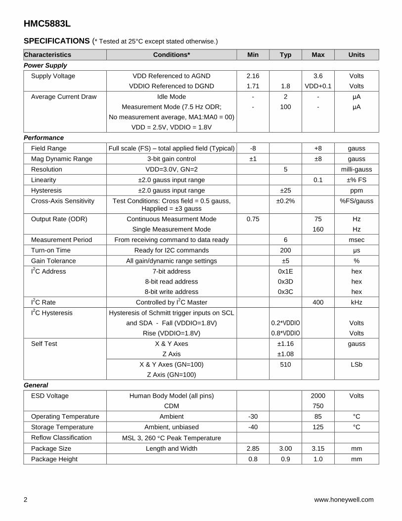
SPECIFICATIONS (* Tested at 25°C except stated otherwise.)

Characteristics Conditions* Min Typ Max Units

Power Supply

Supply Voltage VDD Referenced to AGND

VDDIO Referenced to DGND

2.16

1.71

1.8

3.6

VDD+0.1

Volts

Volts

Average Current Draw Idle Mode

Measurement Mode (7.5 Hz ODR;

No measurement average, MA1:MA0 = 00)

VDD = 2.5V, VDDIO = 1.8V

-

-

2

100

-

-

μA

μA

Performance

Field Range Full scale (FS) – total applied field (Typical) -8 +8 gauss

Mag Dynamic Range 3-bit gain control ±1 ±8 gauss

Resolution VDD=3.0V, GN=2 5 milli-gauss

Linearity ±2.0 gauss input range 0.1 ±% FS

Hysteresis ±2.0 gauss input range ±25 ppm

Cross-Axis Sensitivity Test Conditions: Cross field = 0.5 gauss, Happlied = ±3 gauss

±0.2% %FS/gauss

Output Rate (ODR) Continuous Measurment Mode

Single Measurement Mode

0.75 75

160

Hz

Hz

Measurement Period From receiving command to data ready 6 msec

Turn-on Time Ready for I2C commands 200 μs

Gain Tolerance All gain/dynamic range settings ±5 %

I2C Address 7-bit address

8-bit read address

8-bit write address

0x1E

0x3D

0x3C

hex

hex

hex

I2C Rate Controlled by I

2C Master 400 kHz

I2C Hysteresis Hysteresis of Schmitt trigger inputs on SCL

and SDA - Fall (VDDIO=1.8V)

Rise (VDDIO=1.8V)

0.2*VDDIO

0.8*VDDIO

Volts

Volts

Self Test X & Y Axes

Z Axis

±1.16

±1.08

gauss

X & Y Axes (GN=100)

Z Axis (GN=100)

510 LSb

General

ESD Voltage Human Body Model (all pins)

CDM

2000

750

Volts

Operating Temperature Ambient -30 85 °C

Storage Temperature Ambient, unbiased -40 125 °C

Reflow Classification MSL 3, 260 C Peak Temperature

Package Size Length and Width 2.85 3.00 3.15 mm

Package Height 0.8 0.9 1.0 mm

HMC5883L

www.honeywell.com 3

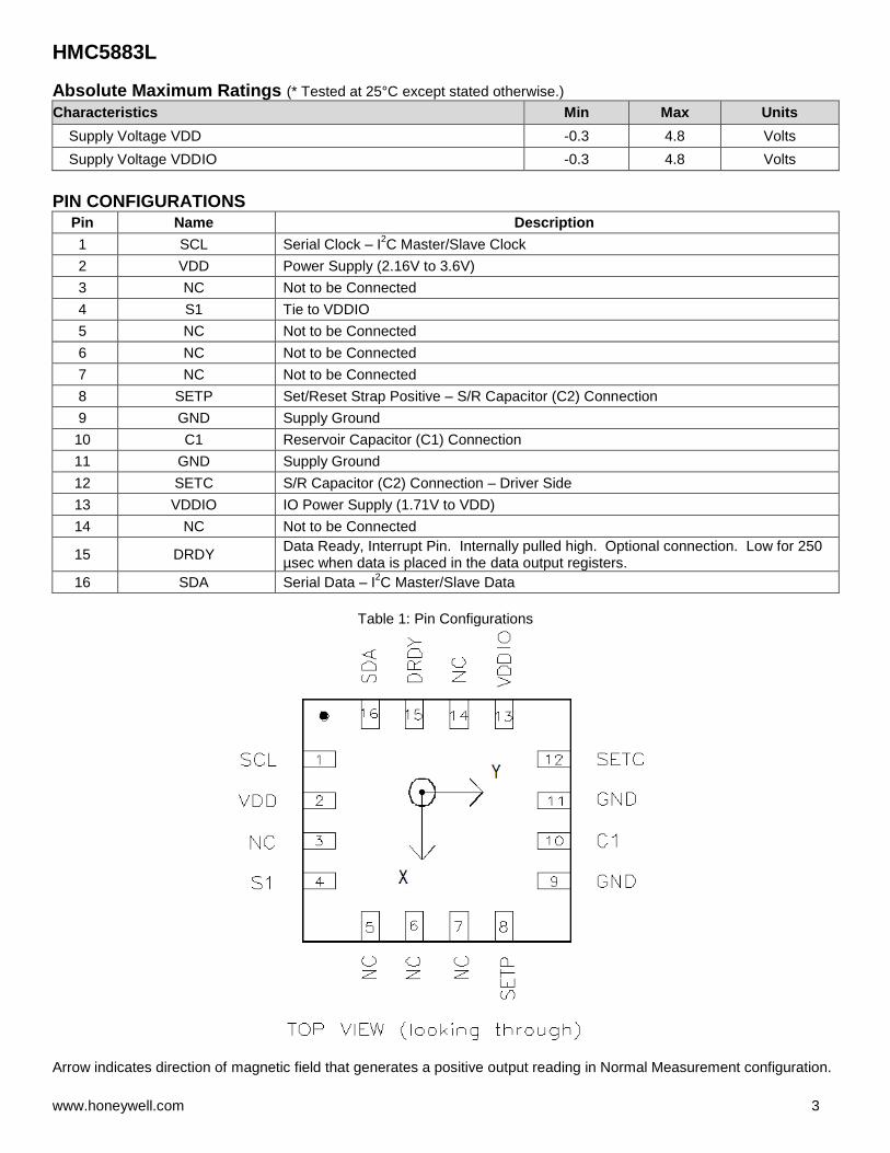
Absolute Maximum Ratings (* Tested at 25°C except stated otherwise.)

Characteristics Min Max Units

Supply Voltage VDD -0.3 4.8 Volts

Supply Voltage VDDIO -0.3 4.8 Volts

PIN CONFIGURATIONS

Pin Name Description

1 SCL Serial Clock – I2C Master/Slave Clock

2 VDD Power Supply (2.16V to 3.6V)

3 NC Not to be Connected

4 S1 Tie to VDDIO

5 NC Not to be Connected

6 NC Not to be Connected

7 NC Not to be Connected

8 SETP Set/Reset Strap Positive – S/R Capacitor (C2) Connection

9 GND Supply Ground

10 C1 Reservoir Capacitor (C1) Connection

11 GND Supply Ground

12 SETC S/R Capacitor (C2) Connection – Driver Side

13 VDDIO IO Power Supply (1.71V to VDD)

14 NC Not to be Connected

15 DRDY Data Ready, Interrupt Pin. Internally pulled high. Optional connection. Low for 250 µsec when data is placed in the data output registers.

16 SDA Serial Data – I2C Master/Slave Data

Table 1: Pin Configurations

Arrow indicates direction of magnetic field that generates a positive output reading in Normal Measurement configuration.

HMC5883L

4 www.honeywell.com

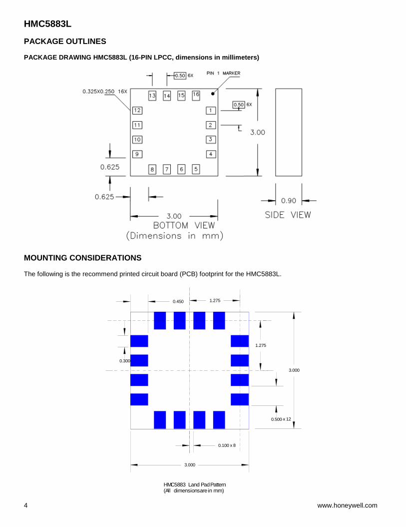
PACKAGE OUTLINES PACKAGE DRAWING HMC5883L (16-PIN LPCC, dimensions in millimeters)

MOUNTING CONSIDERATIONS The following is the recommend printed circuit board (PCB) footprint for the HMC5883L.

0.100

1.275

1.275

0.500

3.000

3.000

0.450

0.300

x 8

x 12

HMC5883 Land Pad Pattern(All dimensions are in mm)

HMC5883L

www.honeywell.com 5

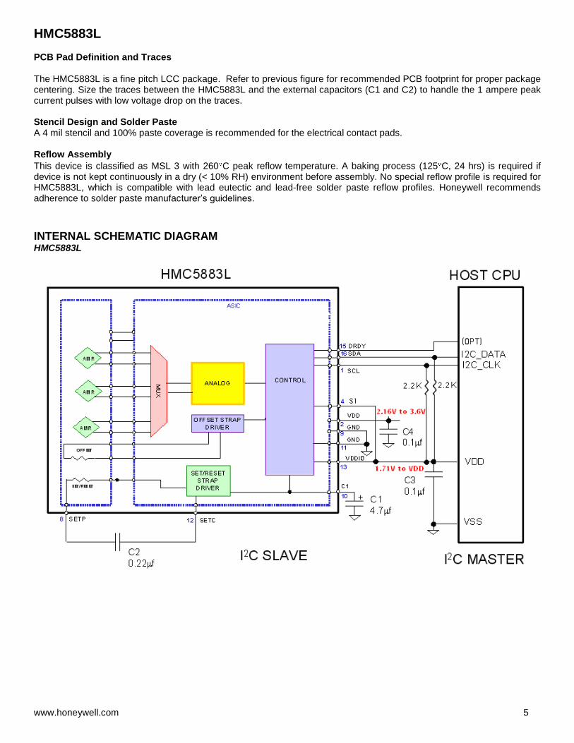
PCB Pad Definition and Traces The HMC5883L is a fine pitch LCC package. Refer to previous figure for recommended PCB footprint for proper package centering. Size the traces between the HMC5883L and the external capacitors (C1 and C2) to handle the 1 ampere peak current pulses with low voltage drop on the traces. Stencil Design and Solder Paste A 4 mil stencil and 100% paste coverage is recommended for the electrical contact pads. Reflow Assembly

This device is classified as MSL 3 with 260 C peak reflow temperature. A baking process (125 C, 24 hrs) is required if device is not kept continuously in a dry (< 10% RH) environment before assembly. No special reflow profile is required for HMC5883L, which is compatible with lead eutectic and lead-free solder paste reflow profiles. Honeywell recommends adherence to solder paste manufacturer’s guidelines.

INTERNAL SCHEMATIC DIAGRAM HMC5883L

HMC5883L

6 www.honeywell.com

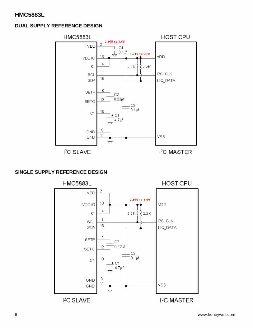
DUAL SUPPLY REFERENCE DESIGN

SINGLE SUPPLY REFERENCE DESIGN

HMC5883L

www.honeywell.com 7

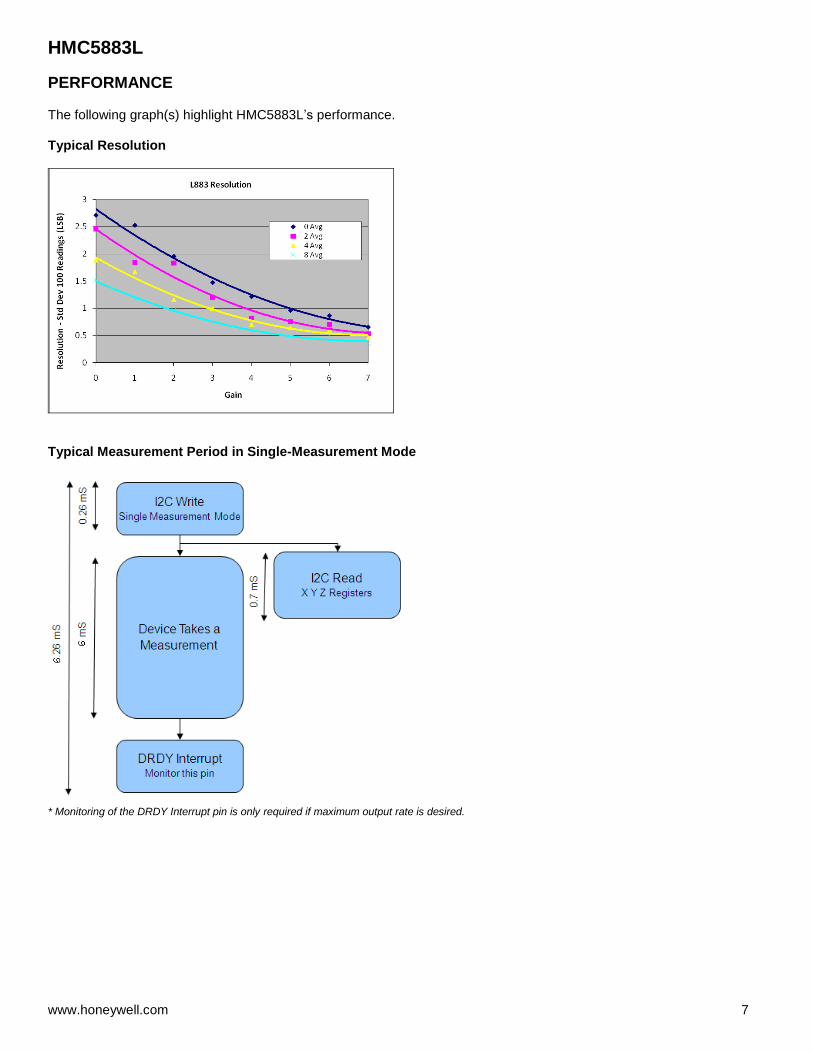
PERFORMANCE

The following graph(s) highlight HMC5883L’s performance. Typical Resolution

Typical Measurement Period in Single-Measurement Mode

* Monitoring of the DRDY Interrupt pin is only required if maximum output rate is desired.

HMC5883L

8 www.honeywell.com

BASIC DEVICE OPERATION Anisotropic Magneto-Resistive Sensors The Honeywell HMC5883L magnetoresistive sensor circuit is a trio of sensors and application specific support circuits to measure magnetic fields. With power supply applied, the sensor converts any incident magnetic field in the sensitive axis directions to a differential voltage output. The magnetoresistive sensors are made of a nickel-iron (Permalloy) thin-film and patterned as a resistive strip element. In the presence of a magnetic field, a change in the bridge resistive elements causes a corresponding change in voltage across the bridge outputs. These resistive elements are aligned together to have a common sensitive axis (indicated by arrows in the pinout diagram) that will provide positive voltage change with magnetic fields increasing in the sensitive direction. Because the output is only proportional to the magnetic field component along its axis, additional sensor bridges are placed at orthogonal directions to permit accurate measurement of magnetic field in any orientation. Self Test To check the HMC5883L for proper operation, a self test feature in incorporated in which the sensor is internally excited with a nominal magnetic field (in either positive or negative bias configuration). This field is then measured and reported. This function is enabled and the polarity is set by bits MS[n] in the configuration register A. An internal current source generates DC current (about 10 mA) from the VDD supply. This DC current is applied to the offset straps of the magneto-resistive sensor, which creates an artificial magnetic field bias on the sensor. See SELF TEST OPERATION section later in this datasheet for additional details. Power Management This device has two different domains of power supply. The first one is VDD that is the power supply for internal operations and the second one is VDDIO that is dedicated to IO interface. It is possible to work with VDDIO equal to VDD; Single Supply mode, or with VDDIO lower than VDD allowing HMC5883L to be compatible with other devices on board. I2C Interface

Control of this device is carried out via the I

2C bus. This device will be connected to this bus as a slave device under the

control of a master device, such as the processor. This device is compliant with I

2C-Bus Specification, document number: 9398 393 40011. As an I

2C compatible device,

this device has a 7-bit serial address and supports I2C protocols. This device supports standard and fast modes, 100kHz

and 400kHz, respectively, but does not support the high speed mode (Hs). External pull-up resistors are required to support these standard and fast speed modes.

Activities required by the master (register read and write) have priority over internal activities, such as the measurement. The purpose of this priority is to not keep the master waiting and the I

2C bus engaged for longer than necessary.

Internal Clock The device has an internal clock for internal digital logic functions and timing management. H-Bridge for Set/Reset Strap Drive The ASIC contains large switching FETs capable of delivering a large but brief pulse to the Set / Reset strap of the sensor. This strap is largely a resistive load. There is no need for an external Set/Reset circuit. The controlling of the Set/Reset function is done automatically by the ASIC for each measurement. One half of the difference from the measurements taken after a set pulse and after a reset pulse will be put in the data output register for each of the three axes. By doing so, the sensor’s internal offset and its temperature dependence is removed/cancelled for all measurements. Charge Current Limit The current that reservoir capacitor (C1) can draw when charging is limited for both single supply and dual supply

HMC5883L

www.honeywell.com 9

configurations. This prevents drawing down the supply voltage (VDD).

MODES OF OPERATION This device has several operating modes whose primary purpose is power management and is controlled by the Mode Register. This section describes these modes. Continuous-Measurement Mode During continuous-measurement mode, the device continuously makes measurements, at user selectable rate, and places measured data in data output registers. Data can be re-read from the data output registers if necessary; however, if the master does not ensure that the data register is accessed before the completion of the next measurement, the data output registers are updated with the new measurement. To conserve current between measurements, the device is placed in a state similar to idle mode, but the Mode Register is not changed to Idle Mode. That is, MD[n] bits are unchanged. Settings in the Configuration Register A affect the data output rate (bits DO[n]), the measurement configuration (bits MS[n]), when in continuous-measurement mode. All registers maintain values while in continuous-measurement mode. The I

2C bus is enabled for use by other devices on the network in while continuous-measurement

mode. Single-Measurement Mode This is the default power-up mode. During single-measurement mode, the device makes a single measurement and places the measured data in data output registers. After the measurement is complete and output data registers are updated, the device is placed in idle mode, and the Mode Register is changed to idle mode by setting MD[n] bits. Settings in the configuration register affect the measurement configuration (bits MS[n])when in single-measurement mode. All registers maintain values while in single-measurement mode. The I

2C bus is enabled for use by other devices on the

network while in single-measurement mode. Idle Mode During this mode the device is accessible through the I

2C bus, but major sources of power consumption are disabled,

such as, but not limited to, the ADC, the amplifier, and the sensor bias current. All registers maintain values while in idle mode. The I

2C bus is enabled for use by other devices on the network while in idle mode.

HMC5883L

10 www.honeywell.com

REGISTERS This device is controlled and configured via a number of on-chip registers, which are described in this section. In the following descriptions, set implies a logic 1, and reset or clear implies a logic 0, unless stated otherwise. Register List The table below lists the registers and their access. All address locations are 8 bits.

Address Location Name Access

00 Configuration Register A Read/Write

01 Configuration Register B Read/Write

02 Mode Register Read/Write

03 Data Output X MSB Register Read

04 Data Output X LSB Register Read

05 Data Output Z MSB Register Read

06 Data Output Z LSB Register Read

07 Data Output Y MSB Register Read

08 Data Output Y LSB Register Read

09 Status Register Read

10 Identification Register A Read

11 Identification Register B Read

12 Identification Register C Read

Table2: Register List

Register Access This section describes the process of reading from and writing to this device. The devices uses an address pointer to indicate which register location is to be read from or written to. These pointer locations are sent from the master to this slave device and succeed the 7-bit address plus 1 bit read/write identifier. To minimize the communication between the master and this device, the address pointer updated automatically without master intervention. This automatic address pointer update has two additional features. First when address 12 or higher is accessed the pointer updates to address 00 and secondly when address 08 is reached, the pointer rolls back to address 03. Logically, the address pointer operation functions as shown below. If (address pointer = 08) then address pointer = 03 Else if (address pointer >= 12) then address pointer = 0 Else (address pointer) = (address pointer) + 1 The address pointer value itself cannot be read via the I

2C bus.

Any attempt to read an invalid address location returns 0’s, and any write to an invalid address location or an undefined bit within a valid address location is ignored by this device. To move the address pointer to a random register location, first issue a “write” to that register location with no data byte following the commend. For example, to move the address pointer to register 10, send 0x3C 0x0A.

HMC5883L

www.honeywell.com 11

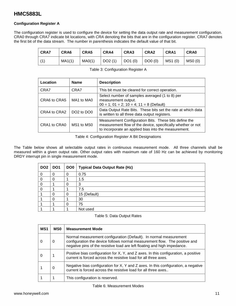
Configuration Register A The configuration register is used to configure the device for setting the data output rate and measurement configuration. CRA0 through CRA7 indicate bit locations, with CRA denoting the bits that are in the configuration register. CRA7 denotes the first bit of the data stream. The number in parenthesis indicates the default value of that bit.

CRA7 CRA6 CRA5 CRA4 CRA3 CRA2 CRA1 CRA0

(1) MA1(1) MA0(1) DO2 (1) DO1 (0) DO0 (0) MS1 (0) MS0 (0)

Table 3: Configuration Register A

Location Name Description

CRA7 CRA7 This bit must be cleared for correct operation.

CRA6 to CRA5 MA1 to MA0 Select number of samples averaged (1 to 8) per measurement output. 00 = 1; 01 = 2; 10 = 4; 11 = 8 (Default)

CRA4 to CRA2 DO2 to DO0 Data Output Rate Bits. These bits set the rate at which data is written to all three data output registers.

CRA1 to CRA0 MS1 to MS0 Measurement Configuration Bits. These bits define the measurement flow of the device, specifically whether or not to incorporate an applied bias into the measurement.

Table 4: Configuration Register A Bit Designations

The Table below shows all selectable output rates in continuous measurement mode. All three channels shall be measured within a given output rate. Other output rates with maximum rate of 160 Hz can be achieved by monitoring DRDY interrupt pin in single measurement mode.

DO2 DO1 DO0 Typical Data Output Rate (Hz)

0 0 0 0.75

0 0 1 1.5

0 1 0 3

0 1 1 7.5

1 0 0 15 (Default)

1 0 1 30

1 1 0 75

1 1 1 Not used

Table 5: Data Output Rates

MS1 MS0 Measurement Mode

0 0 Normal measurement configuration (Default). In normal measurement configuration the device follows normal measurement flow. The positive and negative pins of the resistive load are left floating and high impedance.

0 1 Positive bias configuration for X, Y, and Z axes. In this configuration, a positive current is forced across the resistive load for all three axes.

1 0 Negative bias configuration for X, Y and Z axes. In this configuration, a negative current is forced across the resistive load for all three axes..

1 1 This configuration is reserved.

Table 6: Measurement Modes

HMC5883L

12 www.honeywell.com

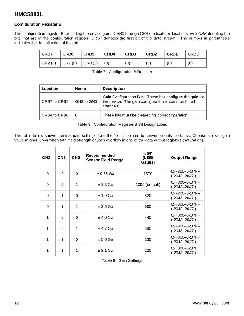
Configuration Register B The configuration register B for setting the device gain. CRB0 through CRB7 indicate bit locations, with CRB denoting the bits that are in the configuration register. CRB7 denotes the first bit of the data stream. The number in parenthesis indicates the default value of that bit.

CRB7 CRB6 CRB5 CRB4 CRB3 CRB2 CRB1 CRB0

GN2 (0) GN1 (0) GN0 (1) (0) (0) (0) (0) (0)

Table 7: Configuration B Register

Location Name Description

CRB7 to CRB5 GN2 to GN0 Gain Configuration Bits. These bits configure the gain for the device. The gain configuration is common for all channels.

CRB4 to CRB0 0 These bits must be cleared for correct operation.

Table 8: Configuration Register B Bit Designations

The table below shows nominal gain settings. Use the “Gain” column to convert counts to Gauss. Choose a lower gain value (higher GN#) when total field strength causes overflow in one of the data output registers (saturation).

GN2 GN1 GN0 Recommended Sensor Field Range

Gain (LSB/

Gauss) Output Range

0 0 0 ± 0.88 Ga 1370 0xF800–0x07FF (-2048–2047 )

0 0 1 ± 1.3 Ga 1090 (default) 0xF800–0x07FF (-2048–2047 )

0 1 0 ± 1.9 Ga 820 0xF800–0x07FF (-2048–2047 )

0 1 1 ± 2.5 Ga 660 0xF800–0x07FF (-2048–2047 )

1 0 0 ± 4.0 Ga 440 0xF800–0x07FF (-2048–2047 )

1 0 1 ± 4.7 Ga 390 0xF800–0x07FF (-2048–2047 )

1 1 0 ± 5.6 Ga 330 0xF800–0x07FF (-2048–2047 )

1 1 1 ± 8.1 Ga 230 0xF800–0x07FF (-2048–2047 )

Table 9: Gain Settings

HMC5883L

www.honeywell.com 13

Mode Register The mode register is an 8-bit register from which data can be read or to which data can be written. This register is used to select the operating mode of the device. MR0 through MR7 indicate bit locations, with MR denoting the bits that are in the mode register. MR7 denotes the first bit of the data stream. The number in parenthesis indicates the default value of that bit.

MR7 MR6 MR5 MR4 MR3 MR2 MR1 MR0

(1) (0) (0) (0) (0) (0) MD1 (0) MD0 (1)

Table 10: Mode Register

Location Name Description

MR7 to MR2

0 These bits must be cleared for correct operation. Bit MR7 bit is set internally after each single-measurement operation.

MR1 to MR0

MD1 to MD0

Mode Select Bits. These bits select the operation mode of this device.

Table 11: Mode Register Bit Designations

MD1 MD0 Operating Mode

0 0

Continuous-Measurement Mode. In continuous-measurement mode, the device continuously performs measurements and places the result in the data register. RDY goes high when new data is placed in all three registers. After a power-on or a write to the mode or configuration register, the first measurement set is available from all three data output registers after a period of 2/fDO and subsequent measurements are available at a frequency of fDO, where fDO is the frequency of data output.

0 1

Single-Measurement Mode (Default). When single-measurement mode is selected, device performs a single measurement, sets RDY high and returned to idle mode. Mode register returns to idle mode bit values. The measurement remains in the data output register and RDY remains high until the data output register is read or another measurement is performed.

1 0 Idle Mode. Device is placed in idle mode.

1 1 Idle Mode. Device is placed in idle mode.

Table 12: Operating Modes

HMC5883L

14 www.honeywell.com

Data Output X Registers A and B The data output X registers are two 8-bit registers, data output register A and data output register B. These registers store the measurement result from channel X. Data output X register A contains the MSB from the measurement result, and data output X register B contains the LSB from the measurement result. The value stored in these two registers is a 16-bit value in 2’s complement form, whose range is 0xF800 to 0x07FF. DXRA0 through DXRA7 and DXRB0 through DXRB7 indicate bit locations, with DXRA and DXRB denoting the bits that are in the data output X registers. DXRA7 and DXRB7 denote the first bit of the data stream. The number in parenthesis indicates the default value of that bit. In the event the ADC reading overflows or underflows for the given channel, or if there is a math overflow during the bias measurement, this data register will contain the value -4096. This register value will clear when after the next valid measurement is made.

DXRA7 DXRA6 DXRA5 DXRA4 DXRA3 DXRA2 DXRA1 DXRA0

(0) (0) (0) (0) (0) (0) (0) (0)

DXRB7 DXRB6 DXRB5 DXRB4 DXRB3 DXRB2 DXRB1 DXRB0

(0) (0) (0) (0) (0) (0) (0) (0)

Table 13: Data Output X Registers A and B

Data Output Y Registers A and B The data output Y registers are two 8-bit registers, data output register A and data output register B. These registers store the measurement result from channel Y. Data output Y register A contains the MSB from the measurement result, and data output Y register B contains the LSB from the measurement result. The value stored in these two registers is a 16-bit value in 2’s complement form, whose range is 0xF800 to 0x07FF. DYRA0 through DYRA7 and DYRB0 through DYRB7 indicate bit locations, with DYRA and DYRB denoting the bits that are in the data output Y registers. DYRA7 and DYRB7 denote the first bit of the data stream. The number in parenthesis indicates the default value of that bit. In the event the ADC reading overflows or underflows for the given channel, or if there is a math overflow during the bias measurement, this data register will contain the value -4096. This register value will clear when after the next valid measurement is made.

DYRA7 DYRA6 DYRA5 DYRA4 DYRA3 DYRA2 DYRA1 DYRA0

(0) (0) (0) (0) (0) (0) (0) (0)

DYRB7 DYRB6 DYRB5 DYRB4 DYRB3 DYRB2 DYRB1 DYRB0

(0) (0) (0) (0) (0) (0) (0) (0)

Table 14: Data Output Y Registers A and B

Data Output Z Registers A and B The data output Z registers are two 8-bit registers, data output register A and data output register B. These registers store the measurement result from channel Z. Data output Z register A contains the MSB from the measurement result, and data output Z register B contains the LSB from the measurement result. The value stored in these two registers is a 16-bit value in 2’s complement form, whose range is 0xF800 to 0x07FF. DZRA0 through DZRA7 and DZRB0 through DZRB7 indicate bit locations, with DZRA and DZRB denoting the bits that are in the data output Z registers. DZRA7 and DZRB7 denote the first bit of the data stream. The number in parenthesis indicates the default value of that bit. In the event the ADC reading overflows or underflows for the given channel, or if there is a math overflow during the bias measurement, this data register will contain the value -4096. This register value will clear when after the next valid measurement is made.

HMC5883L

www.honeywell.com 15

DZRA7 DZRA6 DZRA5 DZRA4 DZRA3 DZRA2 DZRA1 DZRA0

(0) (0) (0) (0) (0) (0) (0) (0)

DZRB7 DZRB6 DZRB5 DZRB4 DZRB3 DZRB2 DZRB1 DZRB0

(0) (0) (0) (0) (0) (0) (0) (0)

Table 15: Data Output Z Registers A and B

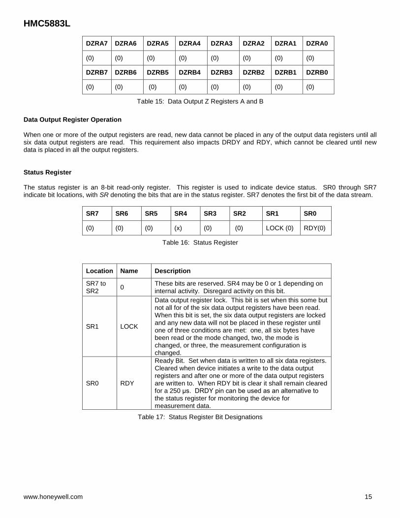
Data Output Register Operation When one or more of the output registers are read, new data cannot be placed in any of the output data registers until all six data output registers are read. This requirement also impacts DRDY and RDY, which cannot be cleared until new data is placed in all the output registers.

Status Register The status register is an 8-bit read-only register. This register is used to indicate device status. SR0 through SR7 indicate bit locations, with SR denoting the bits that are in the status register. SR7 denotes the first bit of the data stream.

SR7 SR6 SR5 SR4 SR3 SR2 SR1 SR0

(0) (0) (0) (x) (0) (0) LOCK (0) RDY(0)

Table 16: Status Register

Location Name Description

SR7 to SR2

0 These bits are reserved. SR4 may be 0 or 1 depending on internal activity. Disregard activity on this bit.

SR1 LOCK

Data output register lock. This bit is set when this some but not all for of the six data output registers have been read. When this bit is set, the six data output registers are locked and any new data will not be placed in these register until one of three conditions are met: one, all six bytes have been read or the mode changed, two, the mode is changed, or three, the measurement configuration is changed.

SR0 RDY

Ready Bit. Set when data is written to all six data registers. Cleared when device initiates a write to the data output registers and after one or more of the data output registers are written to. When RDY bit is clear it shall remain cleared for a 250 μs. DRDY pin can be used as an alternative to the status register for monitoring the device for measurement data.

Table 17: Status Register Bit Designations

HMC5883L

16 www.honeywell.com

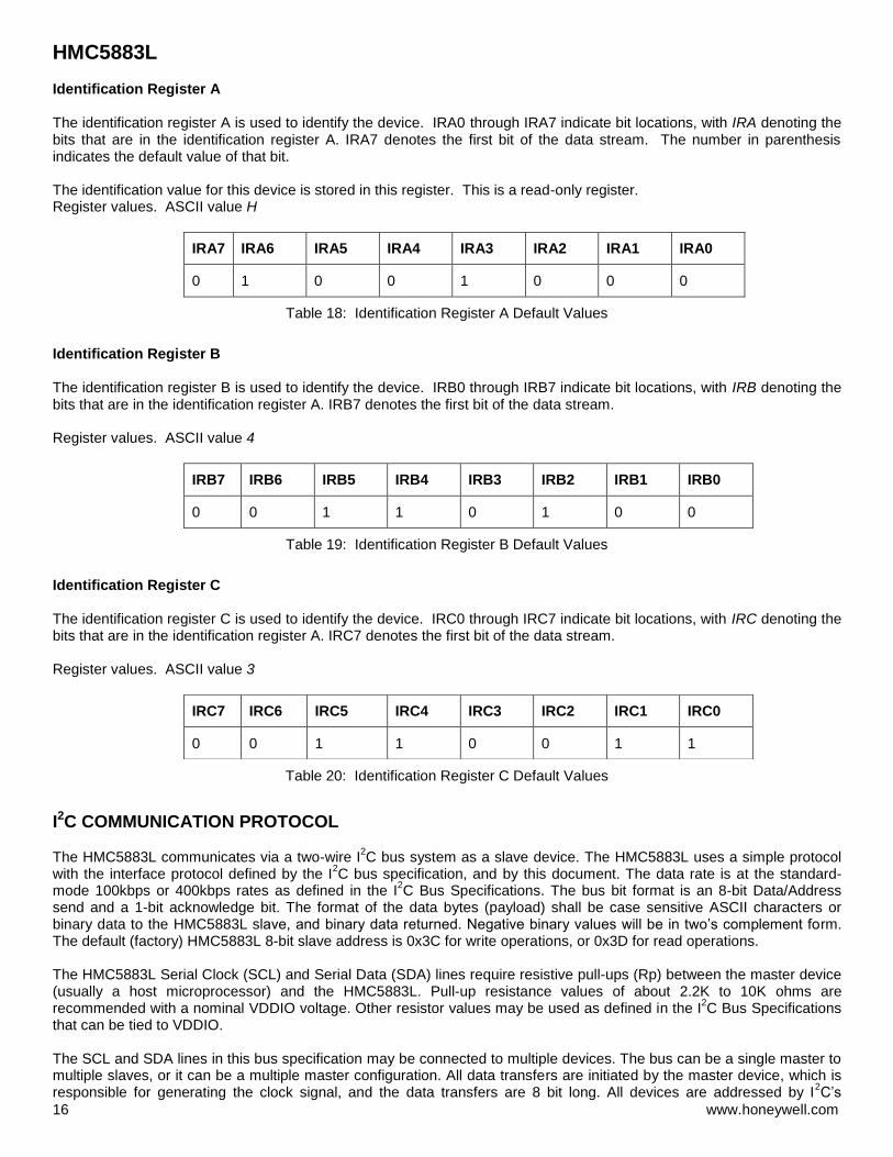
Identification Register A The identification register A is used to identify the device. IRA0 through IRA7 indicate bit locations, with IRA denoting the bits that are in the identification register A. IRA7 denotes the first bit of the data stream. The number in parenthesis indicates the default value of that bit. The identification value for this device is stored in this register. This is a read-only register. Register values. ASCII value H

IRA7 IRA6 IRA5 IRA4 IRA3 IRA2 IRA1 IRA0

0 1 0 0 1 0 0 0

Table 18: Identification Register A Default Values

Identification Register B The identification register B is used to identify the device. IRB0 through IRB7 indicate bit locations, with IRB denoting the bits that are in the identification register A. IRB7 denotes the first bit of the data stream. Register values. ASCII value 4

Table 19: Identification Register B Default Values

Identification Register C The identification register C is used to identify the device. IRC0 through IRC7 indicate bit locations, with IRC denoting the bits that are in the identification register A. IRC7 denotes the first bit of the data stream. Register values. ASCII value 3

Table 20: Identification Register C Default Values

I2C COMMUNICATION PROTOCOL

The HMC5883L communicates via a two-wire I2C bus system as a slave device. The HMC5883L uses a simple protocol

with the interface protocol defined by the I2C bus specification, and by this document. The data rate is at the standard-

mode 100kbps or 400kbps rates as defined in the I2C Bus Specifications. The bus bit format is an 8-bit Data/Address

send and a 1-bit acknowledge bit. The format of the data bytes (payload) shall be case sensitive ASCII characters or binary data to the HMC5883L slave, and binary data returned. Negative binary values will be in two’s complement form. The default (factory) HMC5883L 8-bit slave address is 0x3C for write operations, or 0x3D for read operations. The HMC5883L Serial Clock (SCL) and Serial Data (SDA) lines require resistive pull-ups (Rp) between the master device (usually a host microprocessor) and the HMC5883L. Pull-up resistance values of about 2.2K to 10K ohms are recommended with a nominal VDDIO voltage. Other resistor values may be used as defined in the I

2C Bus Specifications

that can be tied to VDDIO. The SCL and SDA lines in this bus specification may be connected to multiple devices. The bus can be a single master to multiple slaves, or it can be a multiple master configuration. All data transfers are initiated by the master device, which is responsible for generating the clock signal, and the data transfers are 8 bit long. All devices are addressed by I

2C’s

IRB7 IRB6 IRB5 IRB4 IRB3 IRB2 IRB1 IRB0

0 0 1 1 0 1 0 0

IRC7 IRC6 IRC5 IRC4 IRC3 IRC2 IRC1 IRC0

0 0 1 1 0 0 1 1

HMC5883L

www.honeywell.com 17

unique 7-bit address. After each 8-bit transfer, the master device generates a 9th clock pulse, and releases the SDA line.

The receiving device (addressed slave) will pull the SDA line low to acknowledge (ACK) the successful transfer or leave the SDA high to negative acknowledge (NACK). Per the I

2C spec, all transitions in the SDA line must occur when SCL is low. This requirement leads to two unique

conditions on the bus associated with the SDA transitions when SCL is high. Master device pulling the SDA line low while the SCL line is high indicates the Start (S) condition, and the Stop (P) condition is when the SDA line is pulled high while the SCL line is high. The I

2C protocol also allows for the Restart condition in which the master device issues a second

start condition without issuing a stop. All bus transactions begin with the master device issuing the start sequence followed by the slave address byte. The address byte contains the slave address; the upper 7 bits (bits7-1), and the Least Significant bit (LSb). The LSb of the address byte designates if the operation is a read (LSb=1) or a write (LSb=0). At the 9

th clock pulse, the receiving slave

device will issue the ACK (or NACK). Following these bus events, the master will send data bytes for a write operation, or the slave will clock out data with a read operation. All bus transactions are terminated with the master issuing a stop sequence. I2C bus control can be implemented with either hardware logic or in software. Typical hardware designs will release the

SDA and SCL lines as appropriate to allow the slave device to manipulate these lines. In a software implementation, care must be taken to perform these tasks in code.

OPERATIONAL EXAMPLES The HMC5883L has a fairly quick stabilization time from no voltage to stable and ready for data retrieval. The nominal 6 milli-seconds with the factory default single measurement mode means that the six bytes of magnetic data registers (DXRA, DXRB, DZRA, DZRB, DYRA, and DYRB) are filled with a valid first measurement. To change the measurement mode to continuous measurement mode, after the power-up time send the three bytes: 0x3C 0x02 0x00 This writes the 00 into the second register or mode register to switch from single to continuous measurement mode setting. With the data rate at the factory default of 15Hz updates, a 67 milli-second typical delay should be allowed by the I2C master before querying the HMC5883L data registers for new measurements. To clock out the new data, send:

0x3D, and clock out DXRA, DXRB, DZRA, DZRB, DYRA, and DYRB located in registers 3 through 8. The HMC5883L will automatically re-point back to register 3 for the next 0x3D query. All six data registers must be read properly before new data can be placed in any of these data registers.

SELF TEST OPERATION To check the HMC5883L for proper operation, a self test feature in incorporated in which the sensor offset straps are excited to create a nominal field strength (bias field) to be measured. To implement self test, the least significant bits (MS1 and MS0) of configuration register A are changed from 00 to 01 (positive bias) or 10 (negetive bias), e.g. 0x11 or 0x12. Then, by placing the mode register into single-measurement mode (0x01), two data acquisition cycles will be made on each magnetic vector. The first acquisition will be a set pulse followed shortly by measurement data of the external field. The second acquisition will have the offset strap excited (about 10 mA) in the positive bias mode for X, Y, and Z axes to create about a ±1.1 gauss self test field plus the external field. The first acquisition values will be subtracted from the second acquisition, and the net measurement will be placed into the data output registers. Since self test adds ~1.1 Gauss additional field to the existing field strength, using a reduced gain setting prevents sensor from being saturated and data registers overflowed. For example, if the configuration register B is set to 0x60 (Gain=3), values around +766 LSB (1.16 Ga * 660 LSB/Ga) will be placed in the X and Y data output registers and around +713 (1.08 Ga * 660 LSB/Ga) will be placed in Z data output register. To leave the self test mode, change MS1 and MS0 bit of the configuration register A back to 00 (Normal Measurement Mode), e.g. 0x10.

HMC5883L

18 www.honeywell.com

SCALE FACTOR CALIBRATION Using the self test method described above, the user can scale sensors’ sensitivity to match each other. Since placing device in positive bias mode (or alternatively negative bias mode) applies a known artificial field on all three axes, the resulting ADC measurements in data output registers can be used to scale the sensors. For example, if the expected self test value for X-axis is 766 and the actual value is 750 then a scale factor of (766/750) should be multiplied to all future readings of X-axis. Doing so for all three axes will ensure their sensitivity are well matched, The built-in self test can also be used to periodically compensate the scaling errors due to temperature variations. A compensation factor can be found by comparing the self test outputs with the ones obtained at a known temperature. For example, if the self test output is 750 at room temperature and 700 at the current temperature then a compensation factor of (750/700) should be applied to all current magnetic readings. A temperature sensor is not required using this method.

EXTERNAL CAPACITORS The two external capacitors should be ceramic type construction with low ESR characteristics. The exact ESR values are not critical but values less than 200 milli-ohms are recommended. Reservoir capacitor C1 is nominally 4.7 µF in capacitance, with the set/reset capacitor C2 nominally 0.22 µF in capacitance. Low ESR characteristics may not be in many small SMT ceramic capacitors (0402), so be prepared to up-size the capacitors to gain Low ESR characteristics.

ORDERING INFORMATION

Ordering Number Product HMC5883L-TR

Tape and Reel 4k pieces/reel

FIND OUT MORE For more information on Honeywell’s Magnetic Sensors visit us online at www.honeywell.com/magneticsensors or contact us at 800-323-8295 (763-954-2474 internationally). The application circuits herein constitute typical usage and interface of Honeywell product. Honeywell does not warranty or assume liability of customer-designed circuits derived from this description or depiction. Honeywell reserves the right to make changes to improve reliability, function or design. Honeywell does not assume any liability arising out of the application or use of any product or circuit described herein; neither does it convey any license under its patent rights nor the rights of others. U.S. Patents 4,441,072, 4,533,872, 4,569,742, 4,681,812, 4,847,584 and 6,529,114 apply to the technology described

Honeywell 12001 Highway 55 Plymouth, MN 55441 Tel: 800-323-8295 www.honeywell.com/magneticsensors

Form # 900405 Rev B October 2010 ©2010 Honeywell International Inc.

Applications of Magnetoresistive Sensors inNavigation Systems

Michael J. CarusoHoneywell Inc.

ABSTRACT

Most navigation systems today use some type ofcompass to determine heading direction. Using theearthÕs magnetic field, electronic compasses based onmagnetoresistive (MR) sensors can electrically resolvebetter than 0.1 degree rotation. Discussion of a simple 8-point compass will be described using MR sensors.Methods for building a one degree compass using MRsensors will also be discussed. Compensationtechniques are shown to correct for compass tilt anglesand nearby ferrous material disturbances.

INTRODUCTION

The magnetic compass has been used innavigation for centuries. The inventor of the compass isnot known, though evidence suggests that the Chinesewere using lodestoneÑa magnetic iron oreÑover 2000years ago to indicate horizontal directions. It appearsthat Mediterranean seamen of the 12th century were thefirst to use a magnetic compass at sea [1]. Today, thebalanced needle compass is only a slight variation of thisearly discovery. Advances in technology have led to thesolid state electronic compass based on MR magneticsensors and acceleration based tilt sensors. Electroniccompasses offer many advantages over conventionalÒneedleÓ type or gimbaled compasses such as: shockand vibration resistance, electronic compensation forstray field effects, and direct interface to electronicnavigation systems. Two types of compasses will bediscussed in this paperÑa basic eight-point compassand a one-degree compass.

EARTHÕS MAGNETIC FIELD

The earthÕs magnetic field intensity is about 0.5to 0.6 gauss and has a component parallel to the earthÕssurface that always point toward magnetic north. This isthe basis for all magnetic compasses. The key wordshere are Òparallel to the earthÕs surfaceÓ and ÒmagneticnorthÓ.

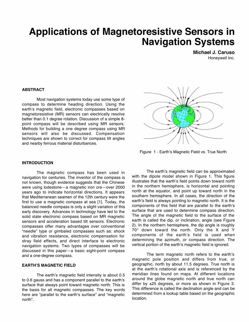
Figure 1 - EarthÕs Magnetic Field vs. True North

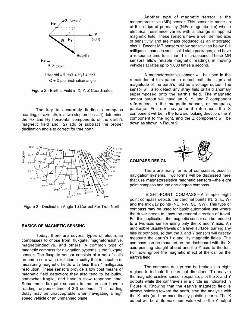
The earthÕs magnetic field can be approximatedwith the dipole model shown in Figure 1. This figureillustrates that the earthÕs field points down toward northin the northern hemisphere, is horizontal and pointingnorth at the equator, and point up toward north in thesouthern hemisphere. In all cases, the direction of theearthÕs field is always pointing to magnetic north. It is thecomponents of this field that are parallel to the earthÕssurface that are used to determine compass direction.The angle of the magnetic field to the surface of theearth is called the dip, or inclination, angle (see Figure2). In the northern hemisphere, the dip angle is roughly70¡ down toward the north. Only the X and Ycomponents of the earthÕs field is used whendetermining the azimuth, or compass direction. Thevertical portion of the earthÕs magnetic field is ignored.

The term magnetic north refers to the earthÕsmagnetic pole position and differs from true, orgeographic, north by about 11.5 degrees. True north isat the earthÕs rotational axis and is referenced by themeridian lines found on maps. At different locationsaround the globe magnetic north and true north candiffer by ±25 degrees, or more as shown in Figure 3.This difference is called the declination angle and can bedetermined from a lookup table based on the geographiclocation.

X (forward)Hx

Hz

Hy

Hearth

¯

Z (down)

Y(right)

¯ = Dip or inclination angle

|Hearth| = Hx2 + Hy2 + Hz2

Figure 2 - EarthÕs Field in X, Y, Z Coordinates

The key to accurately finding a compassheading, or azimuth, is a two step process: 1) determinethe Hx and Hy horizontal components of the earthÕsmagnetic field and 2) add or subtract the properdeclination angle to correct for true north.

22¡E

20¡E

18¡E

16¡E

14¡E

12¡E

10¡E

8¡E6¡E

2¡E0¡

4¡E

2¡W

4¡W

18¡W

16¡W14¡W

12¡W

10¡W

8¡W

6¡W

20¡W22¡W

Figure 3 - Declination Angle To Correct For True North

BASICS OF MAGNETIC SENSING

Today, there are several types of electroniccompasses to chose from: fluxgate, magnetoresistive,magnetoinductive, and others. A common type ofmagnetic compass for navigation systems is the fluxgatesensor. The fluxgate sensor consists of a set of coilsaround a core with excitation circuitry that is capable ofmeasuring magnetic fields with less than 1 milligaussresolution. These sensors provide a low cost means ofmagnetic field detection; they also tend to be bulky,somewhat fragile, and have a slow response time.Sometimes, fluxgate sensors in motion can have areading response time of 2-3 seconds. This readingdelay may be unacceptable when navigating a highspeed vehicle or an unmanned plane.

Another type of magnetic sensor is themagnetoresistive (MR) sensor. This sensor is made upof thin strips of permalloy (NiFe magnetic film) whoseelectrical resistance varies with a change in appliedmagnetic field. These sensors have a well defined axisof sensitivity and are mass produced as an integratedcircuit. Recent MR sensors show sensitivities below 0.1milligauss, come in small solid state packages, and havea response time less than 1 microsecond. These MRsensors allow reliable magnetic readings in movingvehicles at rates up to 1,000 times a second.

A magnetoresistive sensor will be used in theremainder of this paper to detect both the sign andmagnitude of the earthÕs field as a voltage output. Thesensor will also detect any stray field or field anomalysuperimposed onto the earthÕs field. The magneticsensor output will have an X, Y, and Z componentreferenced to the magnetic sensor, or compass,package. For our navigational reference: the Xcomponent will be in the forward looking direction, the Ycomponent to the right, and the Z component will bedown as shown in Figure 2.

COMPASS DESIGN

There are many forms of compasses used innavigation systems. Two forms will be discussed herethat use magnetoresistive magnetic sensorsÑthe eightpoint compass and the one-degree compass.

EIGHT-POINT COMPASSÑA simple eightpoint compass depicts the cardinal points (N, S, E, W)and the midway points (NE, NW, SE, SW). This type ofcompass may be used for basic automotive use wherethe driver needs to know the general direction of travel.For this application, the magnetic sensor can be reducedto a two-axis sensor using only the X and Y axis. Anautomobile usually travels on a level surface, barring anyhills or potholes, so that the X and Y sensors will directlymeasure the earthÕs Hx and Hy magnetic fields. Thecompass can be mounted on the dashboard with the Xaxis pointing straight ahead and the Y axis to the left.For now, ignore the magnetic effect of the car on theearthÕs field.

The compass design can be broken into eightregions to indicate the cardinal directions. To analyzethe magnetoresistive sensor response, plot the X and Youtputs while the car travels in a circle as indicated inFigure 4. Knowing that the earthÕs magnetic field isalways pointing toward the north, start the analysis withthe X axis (and the car) directly pointing north. The Xoutput will be at its maximum value while the Y output

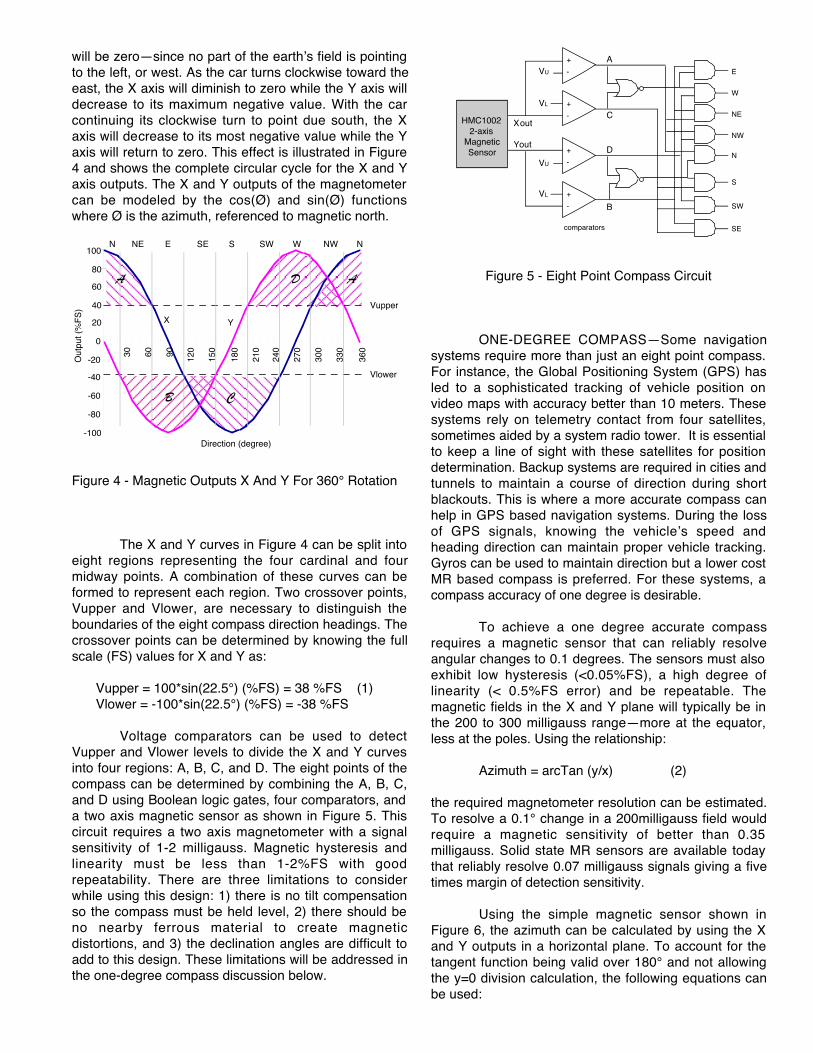
will be zeroÑsince no part of the earthÕs field is pointingto the left, or west. As the car turns clockwise toward theeast, the X axis will diminish to zero while the Y axis willdecrease to its maximum negative value. With the carcontinuing its clockwise turn to point due south, the Xaxis will decrease to its most negative value while the Yaxis will return to zero. This effect is illustrated in Figure4 and shows the complete circular cycle for the X and Yaxis outputs. The X and Y outputs of the magnetometercan be modeled by the cos(¯) and sin(¯) functionswhere ¯ is the azimuth, referenced to magnetic north.

-100

-80

-60

-40

20

40

60

80

100

Direction (degree)

Out

put (

%F

S)

N NE E SE S SW W NW N

X Y

Vupper

Vlower

-20

0

30 60 90

120

150

180

210

240

270

300

330

360

B C

A D A

Figure 4 - Magnetic Outputs X And Y For 360¡ Rotation

The X and Y curves in Figure 4 can be split intoeight regions representing the four cardinal and fourmidway points. A combination of these curves can beformed to represent each region. Two crossover points,Vupper and Vlower, are necessary to distinguish theboundaries of the eight compass direction headings. Thecrossover points can be determined by knowing the fullscale (FS) values for X and Y as:

Vupper = 100*sin(22.5¡) (%FS) = 38 %FS (1)Vlower = -100*sin(22.5¡) (%FS) = -38 %FS

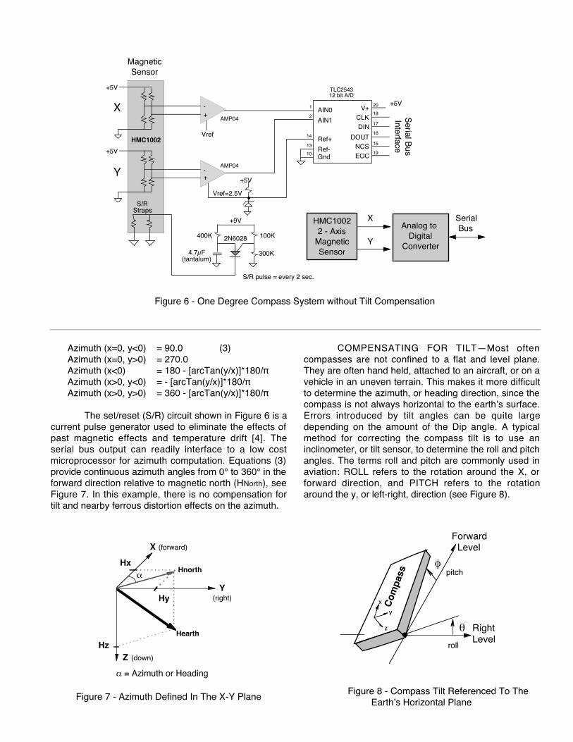
Voltage comparators can be used to detectVupper and Vlower levels to divide the X and Y curvesinto four regions: A, B, C, and D. The eight points of thecompass can be determined by combining the A, B, C,and D using Boolean logic gates, four comparators, anda two axis magnetic sensor as shown in Figure 5. Thiscircuit requires a two axis magnetometer with a signalsensitivity of 1-2 milligauss. Magnetic hysteresis andlinearity must be less than 1-2%FS with goodrepeatability. There are three limitations to considerwhile using this design: 1) there is no tilt compensationso the compass must be held level, 2) there should beno nearby ferrous material to create magneticdistortions, and 3) the declination angles are difficult toadd to this design. These limitations will be addressed inthe one-degree compass discussion below.

VU

E

VL

Yout

NE

NW

N

S

SW

SEcomparators

VU

VL

W

A

C

D

+

-HMC1002

2-axisMagneticSensor +

-

+

-

Xout

B

+

-

Figure 5 - Eight Point Compass Circuit

ONE-DEGREE COMPASSÑSome navigationsystems require more than just an eight point compass.For instance, the Global Positioning System (GPS) hasled to a sophisticated tracking of vehicle position onvideo maps with accuracy better than 10 meters. Thesesystems rely on telemetry contact from four satellites,sometimes aided by a system radio tower. It is essentialto keep a line of sight with these satellites for positiondetermination. Backup systems are required in cities andtunnels to maintain a course of direction during shortblackouts. This is where a more accurate compass canhelp in GPS based navigation systems. During the lossof GPS signals, knowing the vehicleÕs speed andheading direction can maintain proper vehicle tracking.Gyros can be used to maintain direction but a lower costMR based compass is preferred. For these systems, acompass accuracy of one degree is desirable.

To achieve a one degree accurate compassrequires a magnetic sensor that can reliably resolveangular changes to 0.1 degrees. The sensors must alsoexhibit low hysteresis (<0.05%FS), a high degree oflinearity (< 0.5%FS error) and be repeatable. Themagnetic fields in the X and Y plane will typically be inthe 200 to 300 milligauss rangeÑmore at the equator,less at the poles. Using the relationship:

Azimuth = arcTan (y/x) (2)

the required magnetometer resolution can be estimated.To resolve a 0.1¡ change in a 200milligauss field wouldrequire a magnetic sensitivity of better than 0.35milligauss. Solid state MR sensors are available todaythat reliably resolve 0.07 milligauss signals giving a fivetimes margin of detection sensitivity.

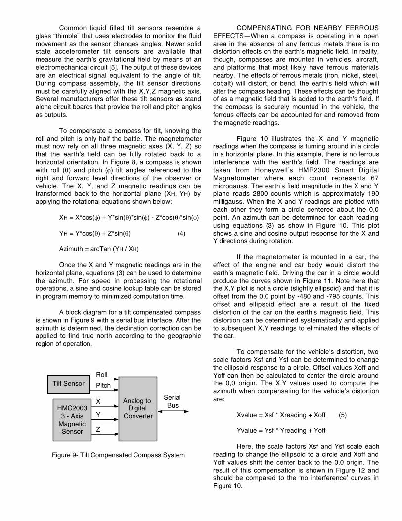
Using the simple magnetic sensor shown inFigure 6, the azimuth can be calculated by using the Xand Y outputs in a horizontal plane. To account for thetangent function being valid over 180¡ and not allowingthe y=0 division calculation, the following equations canbeÊused:

MagneticSensor

+5V

S/RStraps

-+

AMP04

+5V

-+

AMP04

HMC1002

+5V

Vref=2.5V

Vref

X

Y

+9V X

Y

Analog to Digital

Converter

SerialBus

HMC10022 - Axis

MagneticSensor

AIN0

AIN1

Ref+

Ref-

CLKDIN

DOUTNCSEOC

1

2

14

13

18

17

16

15

19

TLC254312 bit A/D

10 Gnd

V+ 20 +5V

Serial B

usInterface

100K

300K

400K

4.7µF(tantalum)

S/R pulse Å every 2 sec.

2N6028

Figure 6 - One Degree Compass System without Tilt Compensation

Azimuth (x=0, y<0) = 90.0 (3)Azimuth (x=0, y>0) = 270.0Azimuth (x<0) = 180 - [arcTan(y/x)]*180/¹Azimuth (x>0, y<0) = - [arcTan(y/x)]*180/¹Azimuth (x>0, y>0) = 360 - [arcTan(y/x)]*180/¹

The set/reset (S/R) circuit shown in Figure 6 is acurrent pulse generator used to eliminate the effects ofpast magnetic effects and temperature drift [4]. Theserial bus output can readily interface to a low costmicroprocessor for azimuth computation. Equations (3)provide continuous azimuth angles from 0¡ to 360¡ in theforward direction relative to magnetic north (HNorth), seeFigure 7. In this example, there is no compensation fortilt and nearby ferrous distortion effects on the azimuth.

X (forward)

Hx

Hz

Hy

Hearth

Z (down)

Y(right)

Hnortha

a = Azimuth or Heading

Figure 7 - Azimuth Defined In The X-Y Plane

COMPENSATING FOR TILTÑMost oftencompasses are not confined to a flat and level plane.They are often hand held, attached to an aircraft, or on avehicle in an uneven terrain. This makes it more difficultto determine the azimuth, or heading direction, since thecompass is not always horizontal to the earthÕs surface.Errors introduced by tilt angles can be quite largedepending on the amount of the Dip angle. A typicalmethod for correcting the compass tilt is to use aninclinometer, or tilt sensor, to determine the roll and pitchangles. The terms roll and pitch are commonly used inaviation: ROLL refers to the rotation around the X, orforward direction, and PITCH refers to the rotationaround the y, or left-right, direction (see Figure 8).

f

q

ForwardLevel

roll

pitch

Com

pass

RightLevel

x

y

z

Figure 8 - Compass Tilt Referenced To TheEarthÕs Horizontal Plane

Common liquid filled tilt sensors resemble aglass ÒthimbleÓ that uses electrodes to monitor the fluidmovement as the sensor changes angles. Newer solidstate accelerometer tilt sensors are available thatmeasure the earthÕs gravitational field by means of anelectromechanical circuit [5]. The output of these devicesare an electrical signal equivalent to the angle of tilt.During compass assembly, the tilt sensor directionsmust be carefully aligned with the X,Y,Z magnetic axis.Several manufacturers offer these tilt sensors as standalone circuit boards that provide the roll and pitch anglesas outputs.

To compensate a compass for tilt, knowing theroll and pitch is only half the battle. The magnetometermust now rely on all three magnetic axes (X, Y, Z) sothat the earthÕs field can be fully rotated back to ahorizontal orientation. In Figure 8, a compass is shownwith roll (q) and pitch (f) tilt angles referenced to theright and forward level directions of the observer orvehicle. The X, Y, and Z magnetic readings can betransformed back to the horizontal plane (XH, YH) byapplying the rotational equations shown below:

XH = X*cos(f) + Y*sin(q)*sin(f) - Z*cos(q)*sin(f)

YH = Y*cos(q) + Z*sin(q) (4)

Azimuth = arcTan (YH / XH)

Once the X and Y magnetic readings are in thehorizontal plane, equations (3) can be used to determinethe azimuth. For speed in processing the rotationaloperations, a sine and cosine lookup table can be storedin program memory to minimized computation time.

A block diagram for a tilt compensated compassis shown in Figure 9 with a serial bus interface. After theazimuth is determined, the declination correction can beapplied to find true north according to the geographicregion of operation.

X

YHMC2003

3 - AxisMagneticSensor

Analog to Digital

Converter

SerialBus

Tilt Sensor Pitch

Roll

Z

Figure 9- Tilt Compensated Compass System

COMPENSATING FOR NEARBY FERROUSEFFECTSÑWhen a compass is operating in a openarea in the absence of any ferrous metals there is nodistortion effects on the earthÕs magnetic field. In reality,though, compasses are mounted in vehicles, aircraft,and platforms that most likely have ferrous materialsnearby. The effects of ferrous metals (iron, nickel, steel,cobalt) will distort, or bend, the earthÕs field which willalter the compass heading. These effects can be thoughtof as a magnetic field that is added to the earthÕs field. Ifthe compass is securely mounted in the vehicle, theferrous effects can be accounted for and removed fromthe magnetic readings.

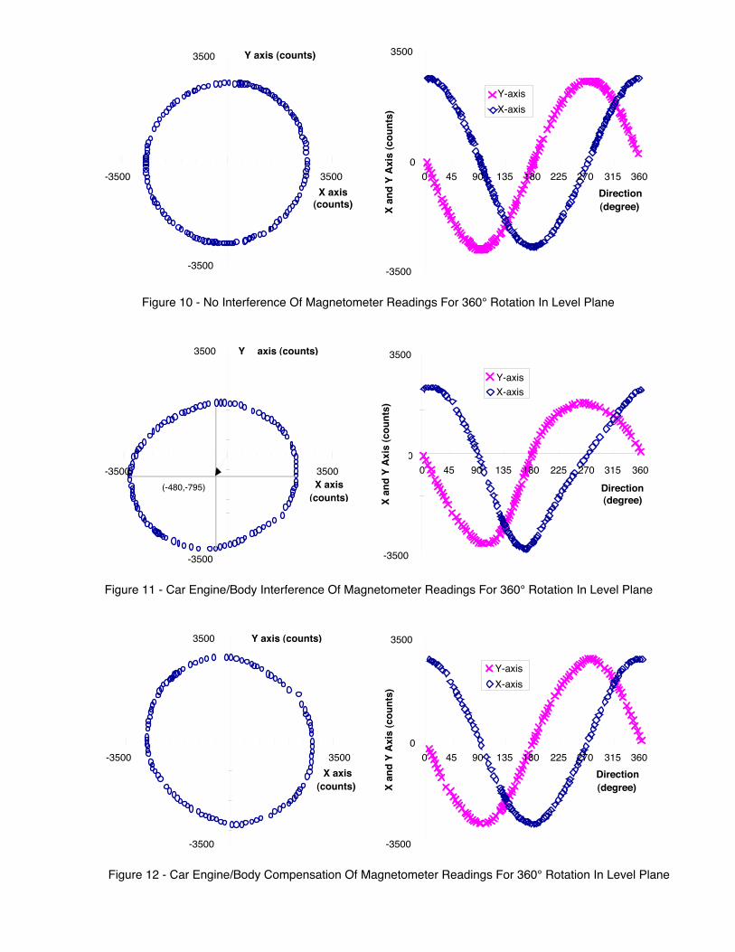
Figure 10 illustrates the X and Y magneticreadings when the compass is turning around in a circlein a horizontal plane. In this example, there is no ferrousinterference with the earthÕs field. The readings aretaken from HoneywellÕs HMR2300 Smart DigitalMagnetometer where each count represents 67microgauss. The earthÕs field magnitude in the X and Yplane reads 2800 counts which is approximately 190milligauss. When the X and Y readings are plotted witheach other they form a circle centered about the 0,0point. An azimuth can be determined for each readingusing equations (3) as show in Figure 10. This plotshows a sine and cosine output response for the X andY directions during rotation.

If the magnetometer is mounted in a car, theeffect of the engine and car body would distort theearthÕs magnetic field. Driving the car in a circle wouldproduce the curves shown in Figure 11. Note here thatthe X,Y plot is not a circle (slightly ellipsoid) and that it isoffset from the 0,0 point by -480 and -795 counts. Thisoffset and ellipsoid effect are a result of the fixeddistortion of the car on the earthÕs magnetic field. Thisdistortion can be determined systematically and appliedto subsequent X,Y readings to eliminated the effects ofthe car.

To compensate for the vehicleÕs distortion, twoscale factors Xsf and Ysf can be determined to changethe ellipsoid response to a circle. Offset values Xoff andYoff can then be calculated to center the circle aroundthe 0,0 origin. The X,Y values used to compute theazimuth when compensating for the vehicleÕs distortionare:

Xvalue = Xsf * Xreading + Xoff (5)

Yvalue = Ysf * Yreading + Yoff

Here, the scale factors Xsf and Ysf scale eachreading to change the ellipsoid to a circle and Xoff andYoff values shift the center back to the 0,0 origin. Theresult of this compensation is shown in Figure 12 andshould be compared to the Ôno interferenceÕ curves inFigure 10.

-3500

0

3500

0 45 90 135 180 225 270 315 360

Direction(degree)X

an

d Y

Axi

s (c

ou

nts

)

Y-axis

X-axis

-3500

3500

-3500 3500

X axis(counts)

Y axis (counts)

Figure 10 - No Interference Of Magnetometer Readings For 360¡ Rotation In Level Plane

-3500

0

3500

0 45 90 135 180 225 270 315 360

Direction(degree)X

an

d Y

Axi

s (c

ou

nts

)Y-axis

X-axis

-3500

3500

-3500 3500

(-480,-795) X axis(counts)

Y axis (counts)

Figure 11 - Car Engine/Body Interference Of Magnetometer Readings For 360¡ Rotation In Level Plane

-3500

0

3500

0 45 90 135 180 225 270 315 360

Direction(degree)X

an

d Y

Axi

s (c

ou

nts

)

Y-axis

X-axis

-3500

3500

-3500 3500

X axis(counts)

Y axis (counts)

Figure 12 - Car Engine/Body Compensation Of Magnetometer Readings For 360¡ Rotation In Level Plane

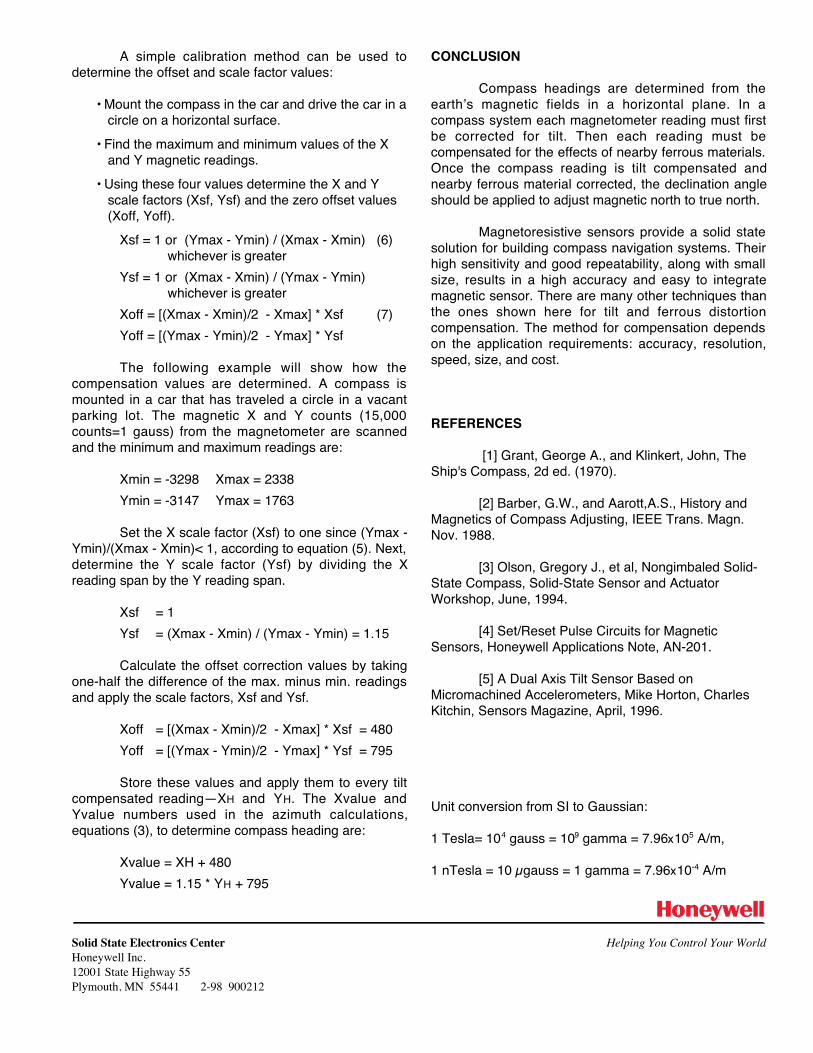
A simple calibration method can be used todetermine the offset and scale factor values:

¥ Mount the compass in the car and drive the car in acircle on a horizontal surface.

¥ Find the maximum and minimum values of the Xand Y magnetic readings.

¥ Using these four values determine the X and Yscale factors (Xsf, Ysf) and the zero offset values(Xoff, Yoff).

Xsf = 1 or (Ymax - Ymin) / (Xmax - Xmin) (6)whichever is greater

Ysf = 1 or (Xmax - Xmin) / (Ymax - Ymin) whichever is greater

Xoff = [(Xmax - Xmin)/2 - Xmax] * Xsf (7)

Yoff = [(Ymax - Ymin)/2 - Ymax] * Ysf

The following example will show how thecompensation values are determined. A compass ismounted in a car that has traveled a circle in a vacantparking lot. The magnetic X and Y counts (15,000counts=1 gauss) from the magnetometer are scannedand the minimum and maximum readings are:

Xmin = -3298 Xmax = 2338

Ymin = -3147 Ymax = 1763

Set the X scale factor (Xsf) to one since (Ymax -Ymin)/(Xmax - Xmin)< 1, according to equation (5). Next,determine the Y scale factor (Ysf) by dividing the Xreading span by the Y reading span.

Xsf = 1

Ysf = (Xmax - Xmin) / (Ymax - Ymin) = 1.15

Calculate the offset correction values by takingone-half the difference of the max. minus min. readingsand apply the scale factors, Xsf and Ysf.

Xoff = [(Xmax - Xmin)/2 - Xmax] * Xsf = 480

Yoff = [(Ymax - Ymin)/2 - Ymax] * Ysf = 795

Store these values and apply them to every tiltcompensated readingÑXH and YH. The Xvalue andYvalue numbers used in the azimuth calculations,equations (3), to determine compass heading are:

Xvalue = XH + 480

Yvalue = 1.15 * YH + 795

CONCLUSION

Compass headings are determined from theearthÕs magnetic fields in a horizontal plane. In acompass system each magnetometer reading must firstbe corrected for tilt. Then each reading must becompensated for the effects of nearby ferrous materials.Once the compass reading is tilt compensated andnearby ferrous material corrected, the declination angleshould be applied to adjust magnetic north to true north.

Magnetoresistive sensors provide a solid statesolution for building compass navigation systems. Theirhigh sensitivity and good repeatability, along with smallsize, results in a high accuracy and easy to integratemagnetic sensor. There are many other techniques thanthe ones shown here for tilt and ferrous distortioncompensation. The method for compensation dependson the application requirements: accuracy, resolution,speed, size, and cost.

REFERENCES

[1] Grant, George A., and Klinkert, John, TheShip's Compass, 2d ed. (1970).

[2] Barber, G.W., and Aarott,A.S., History andMagnetics of Compass Adjusting, IEEE Trans. Magn.Nov. 1988.

[3] Olson, Gregory J., et al, Nongimbaled Solid-State Compass, Solid-State Sensor and ActuatorWorkshop, June, 1994.

[4] Set/Reset Pulse Circuits for MagneticSensors, Honeywell Applications Note, AN-201.

[5] A Dual Axis Tilt Sensor Based onMicromachined Accelerometers, Mike Horton, CharlesKitchin, Sensors Magazine, April, 1996.

Unit conversion from SI to Gaussian:

1 Tesla= 104 gauss = 109 gamma = 7.96x105 A/m,

1 nTesla = 10 µgauss = 1 gamma = 7.96x10-4 A/m

Solid State Electronics Center Helping You Control Your WorldHoneywell Inc.12001 State Highway 55Plymouth, MN 55441 2-98 900212

1

Applications of Magnetic Sensors forLow Cost Compass Systems

Michael J. CarusoHoneywell, SSEC

Abstract—A method for heading determination isdescribed here that will include the effects of pitch and rollas well as the magnetic properties of the vehicle. Usingsolid-state magnetic sensors and a tilt sensor, a low-costcompass system can be realized. Commercial airlinestoday use attitude and heading reference systems that costtens of thousands of dollars. For general aviation, or smallprivate aircraft, this is too costly for most pilots' budget.The compass system described here will provide heading,pitch and roll outputs accurate to one degree, or better.The shortfall of this low-cost approach is that the compassoutputs are affected by acceleration and turns. A solutionto this problem is presented at the end of this paper.

BACKGROUND

The Earth’s magnetic field intensity is about 0.5 to 0.6gauss and has a component parallel to the Earth’s surfacethat always point toward magnetic north. This field can beapproximated with a dipole model—the field points downtoward north in the Northern Hemisphere, is horizontaland pointing north at the equator, and point up towardnorth in the Southern Hemisphere. In all cases, thehorizontal direction of the Earth’s field is always pointingtoward magnetic north and is used to determine compassdirection.

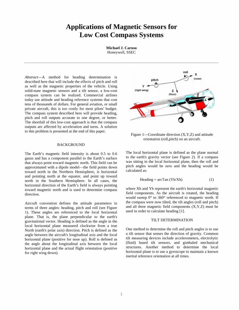
Aircraft convention defines the attitude parameters interms of three angles: heading, pitch and roll (see Figure1). These angles are referenced to the local horizontalplane. That is, the plane perpendicular to the earth'sgravitational vector. Heading is defined as the angle in thelocal horizontal plane measured clockwise from a trueNorth (earth's polar axis) direction. Pitch is defined as theangle between the aircraft's longitudinal axis and the localhorizontal plane (positive for nose up). Roll is defined asthe angle about the longitudinal axis between the localhorizontal plane and the actual flight orientation (positivefor right wing down).

Figure 1—Coordinate direction (X,Y,Z) and attitudeorientation (roll,pitch) on an aircraft.

The local horizontal plane is defined as the plane normalto the earth's gravity vector (see Figure 2). If a compasswas sitting in the local horizontal plane, then the roll andpitch angles would be zero and the heading would becalculated as:

Heading = arcTan (Yh/Xh) (1)

where Xh and Yh represent the earth's horizontal magneticfield components. As the aircraft is rotated, the headingwould sweep 0° to 360° referenced to magnetic north. Ifthe compass were now tilted, the tilt angles (roll and pitch)and all three magnetic field components (X,Y,Z) must beused in order to calculate heading [1].

TILT DETERMINATION

One method to determine the roll and pitch angles is to usea tilt sensor that senses the direction of gravity. Commontilt measuring devices include accelerometers, electrolytic(fluid) based tilt sensors, and gimbaled mechanicalstructures. Another method to determine the localhorizontal plane is to use a gyroscope to maintain a knowninertial reference orientation at all times.

2

gravityvector

local horizontal plane

pitch-roll

tilt sensor

Xh

YhX

Y3 - AxisMagneticSensor

Analog to Digital

Converter

Tilt compensatedazimuth or heading

Tilt Sensor Pitch

Roll

Z

µProcessorinterface and

algorithm

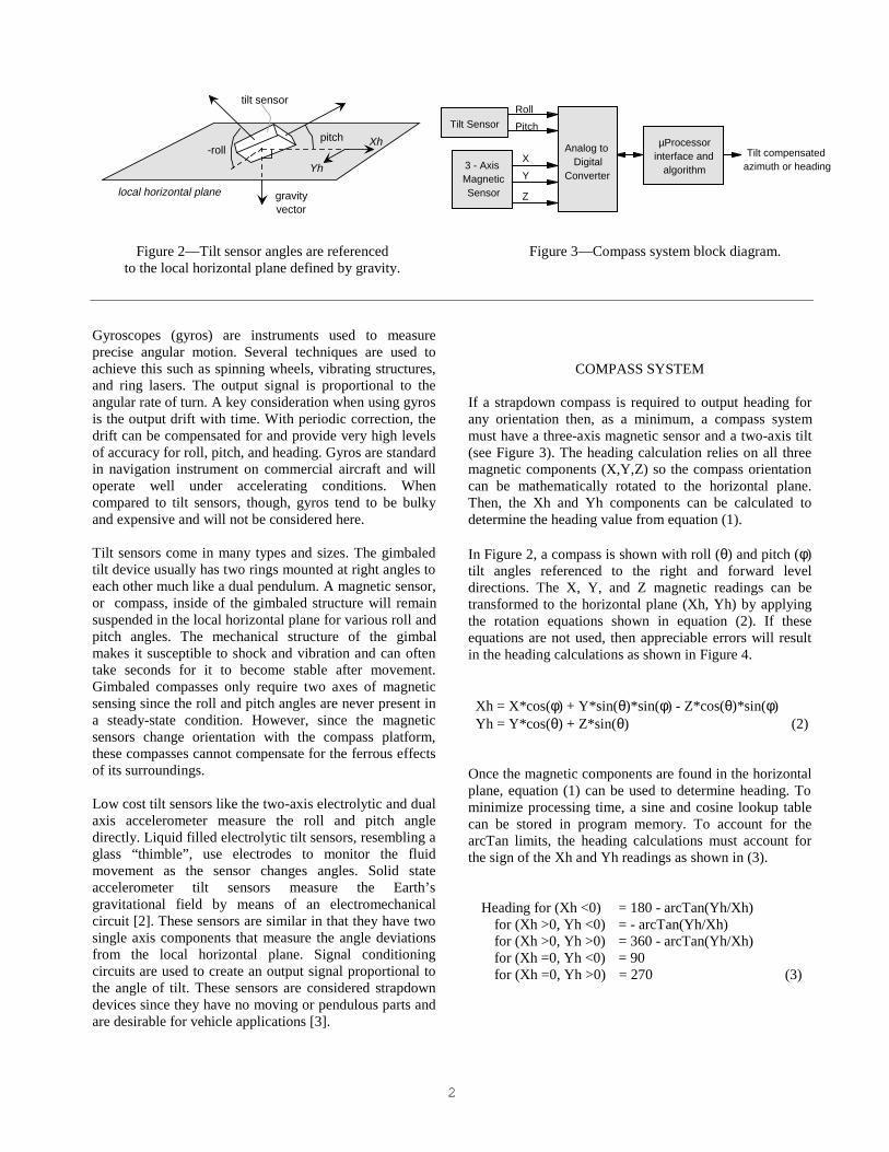
Figure 2—Tilt sensor angles are referenced Figure 3—Compass system block diagram.to the local horizontal plane defined by gravity.

Gyroscopes (gyros) are instruments used to measureprecise angular motion. Several techniques are used toachieve this such as spinning wheels, vibrating structures,and ring lasers. The output signal is proportional to theangular rate of turn. A key consideration when using gyrosis the output drift with time. With periodic correction, thedrift can be compensated for and provide very high levelsof accuracy for roll, pitch, and heading. Gyros are standardin navigation instrument on commercial aircraft and willoperate well under accelerating conditions. Whencompared to tilt sensors, though, gyros tend to be bulkyand expensive and will not be considered here.

Tilt sensors come in many types and sizes. The gimbaledtilt device usually has two rings mounted at right angles toeach other much like a dual pendulum. A magnetic sensor,or compass, inside of the gimbaled structure will remainsuspended in the local horizontal plane for various roll andpitch angles. The mechanical structure of the gimbalmakes it susceptible to shock and vibration and can oftentake seconds for it to become stable after movement.Gimbaled compasses only require two axes of magneticsensing since the roll and pitch angles are never present ina steady-state condition. However, since the magneticsensors change orientation with the compass platform,these compasses cannot compensate for the ferrous effectsof its surroundings.

Low cost tilt sensors like the two-axis electrolytic and dualaxis accelerometer measure the roll and pitch angledirectly. Liquid filled electrolytic tilt sensors, resembling aglass “thimble”, use electrodes to monitor the fluidmovement as the sensor changes angles. Solid stateaccelerometer tilt sensors measure the Earth’sgravitational field by means of an electromechanicalcircuit [2]. These sensors are similar in that they have twosingle axis components that measure the angle deviationsfrom the local horizontal plane. Signal conditioningcircuits are used to create an output signal proportional tothe angle of tilt. These sensors are considered strapdowndevices since they have no moving or pendulous parts andare desirable for vehicle applications [3].

COMPASS SYSTEM

If a strapdown compass is required to output heading forany orientation then, as a minimum, a compass systemmust have a three-axis magnetic sensor and a two-axis tilt(see Figure 3). The heading calculation relies on all threemagnetic components (X,Y,Z) so the compass orientationcan be mathematically rotated to the horizontal plane.Then, the Xh and Yh components can be calculated todetermine the heading value from equation (1).

In Figure 2, a compass is shown with roll (θ) and pitch (φ)tilt angles referenced to the right and forward leveldirections. The X, Y, and Z magnetic readings can betransformed to the horizontal plane (Xh, Yh) by applyingthe rotation equations shown in equation (2). If theseequations are not used, then appreciable errors will resultin the heading calculations as shown in Figure 4.

Xh = X*cos(φ) + Y*sin(θ)*sin(φ) - Z*cos(θ)*sin(φ) Yh = Y*cos(θ) + Z*sin(θ) (2)

Once the magnetic components are found in the horizontalplane, equation (1) can be used to determine heading. Tominimize processing time, a sine and cosine lookup tablecan be stored in program memory. To account for thearcTan limits, the heading calculations must account forthe sign of the Xh and Yh readings as shown in (3).

Heading for (Xh <0) = 180 - arcTan(Yh/Xh)for (Xh >0, Yh <0) = - arcTan(Yh/Xh)for (Xh >0, Yh >0) = 360 - arcTan(Yh/Xh)for (Xh =0, Yh <0) = 90for (Xh =0, Yh >0) = 270 (3)

3

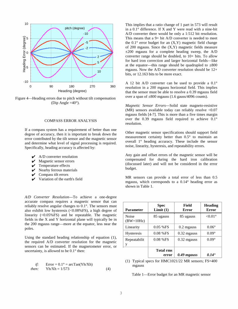
Figure 4—Heading errors due to pitch without tilt compensation(Dip Angle =40°).

COMPASS ERROR ANALYSIS

If a compass system has a requirement of better than onedegree of accuracy, then it is important to break down theerror contributed by the tilt sensor and the magnetic sensorand determine what level of signal processing is required.Specifically, heading accuracy is affected by:

✔ A/D converter resolution✔ Magnetic sensor errors✔ Temperature effects✔ Nearby ferrous materials✔ Compass tilt errors✔ Variation of the earth's field

A/D Converter Resolution—To achieve a one-degreeaccurate compass requires a magnetic sensor that canreliably resolve angular changes to 0.1°. The sensors mustalso exhibit low hysteresis (<0.08%FS), a high degree oflinearity (<0.05%FS) and be repeatable. The magneticfields in the X and Y horizontal plane will typically be inthe 200 mgauss range—more at the equator, less near thepoles.

Using the standard heading relationship of equation (1),the required A/D converter resolution for the magneticsensors can be estimated. If the magnetometer error, oruncertainty, is allowed to be 0.1° then:

if: Error = 0.1° = arcTan(Yh/Xh)then: Yh/Xh = 1/573 (4)

This implies that a ratio change of 1 part in 573 will resultin a 0.1° difference. If X and Y were read with a nine-bitA/D converter there would be only a 1:512 bit resolution.This means that a 9+ bit A/D converter is needed to meetthe 0.1° error budget for an (X,Y) magnetic field changeof 200 mgauss. Since the (X,Y) magnetic fields measure±200 mgauss for a complete heading sweep, the A/Dconverter range should be doubled, to 10+ bits. To allowfor hard iron correction and larger horizontal fields—likeat the equator—this range should be quadrupled to ±800mgauss. Now the A/D converter resolution should be 12+bits, or 12.163 bits to be more exact.

A 12 bit A/D converter can be used to provide a 0.1°resolution in a 200 mgauss horizontal field. This impliesthat the sensor must be able to resolve a 0.39 mgauss fieldover a span of ±800 mgauss (1.6 gauss/4096 counts).

Magnetic Sensor Errors—Solid state magneto-resistive(MR) sensors available today can reliably resolve <0.07mgauss fields [4-7]. This is more than a five times marginover the 0.39 mgauss field required to achieve 0.1°resolution.

Other magnetic sensor specifications should support fieldmeasurement certainty better than 0.5° to maintain anoverall 1° heading accuracy. These include the sensornoise, linearity, hysteresis, and repeatability errors.

Any gain and offset errors of the magnetic sensor will becompensated for during the hard iron calibration(discussed later) and will not be considered in the errorbudget.

MR sensors can provide a total error of less than 0.5mgauss, which corresponds to a 0.14° heading error asshown in Table 1.

ParameterSpec

Limit (1)FieldError

HeadingError

Noise(BW=10Hz)

85 ugauss 85 ugauss <0.01°

Linearity 0.05 %FS 0.2 mgauss 0.06°

Hysteresis 0.08 %FS 0.32 mgauss 0.09°

Repeatability

0.08 %FS 0.32 mgauss 0.09°

Total rmserror 0.49 mgauss 0.14°

(1) Typical specs for HMC1021/22 MR sensors; FS=400mgauss

Table 1—Error budget for an MR magnetic sensor

-10

-5

0

5

10

0 90 180 270 360Heading (degree)

Hea

ding

Err

or (

degr

ee)

pitch (degree)

-10

-5

-2

2

5

10

4

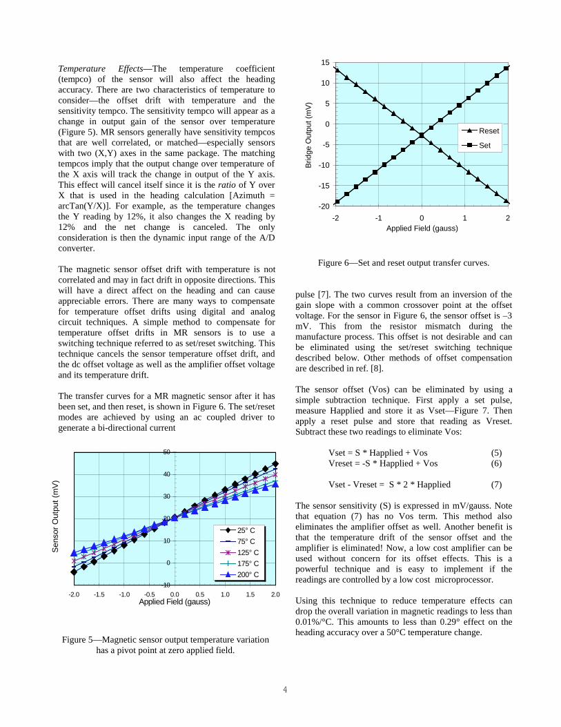
Temperature Effects—The temperature coefficient(tempco) of the sensor will also affect the headingaccuracy. There are two characteristics of temperature toconsider—the offset drift with temperature and thesensitivity tempco. The sensitivity tempco will appear as achange in output gain of the sensor over temperature(Figure 5). MR sensors generally have sensitivity tempcosthat are well correlated, or matched—especially sensorswith two (X,Y) axes in the same package. The matchingtempcos imply that the output change over temperature ofthe X axis will track the change in output of the Y axis.This effect will cancel itself since it is the ratio of Y overX that is used in the heading calculation [Azimuth =arcTan(Y/X)]. For example, as the temperature changesthe Y reading by 12%, it also changes the X reading by12% and the net change is canceled. The onlyconsideration is then the dynamic input range of the A/Dconverter.

The magnetic sensor offset drift with temperature is notcorrelated and may in fact drift in opposite directions. Thiswill have a direct affect on the heading and can causeappreciable errors. There are many ways to compensatefor temperature offset drifts using digital and analogcircuit techniques. A simple method to compensate fortemperature offset drifts in MR sensors is to use aswitching technique referred to as set/reset switching. Thistechnique cancels the sensor temperature offset drift, andthe dc offset voltage as well as the amplifier offset voltageand its temperature drift.

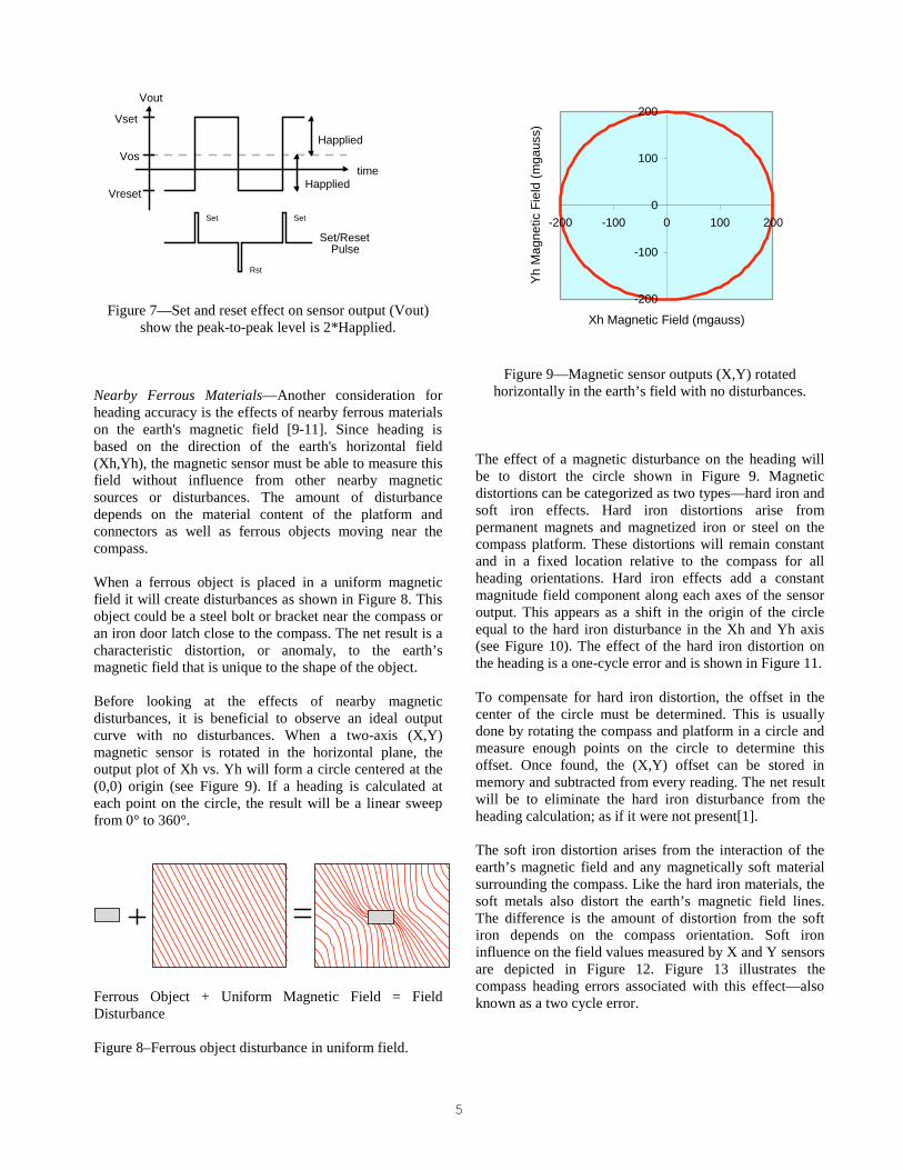
The transfer curves for a MR magnetic sensor after it hasbeen set, and then reset, is shown in Figure 6. The set/resetmodes are achieved by using an ac coupled driver togenerate a bi-directional current

-10

0

10

20

30

40

50

-2.0 -1.5 -1.0 -0.5 0.0 0.5 1.0 1.5 2.0Applied Field (gauss)

Sen

sor

Out

put (

mV

)

25° C

75° C

125° C

175° C

200° C

Figure 5—Magnetic sensor output temperature variationhas a pivot point at zero applied field.

-20

-15

-10

-5

0

5

10

15

-2 -1 0 1 2Applied Field (gauss)

Brid

ge O

utpu

t (m

V)

Reset

Set

Figure 6—Set and reset output transfer curves.

pulse [7]. The two curves result from an inversion of thegain slope with a common crossover point at the offsetvoltage. For the sensor in Figure 6, the sensor offset is –3mV. This from the resistor mismatch during themanufacture process. This offset is not desirable and canbe eliminated using the set/reset switching techniquedescribed below. Other methods of offset compensationare described in ref. [8].

The sensor offset (Vos) can be eliminated by using asimple subtraction technique. First apply a set pulse,measure Happlied and store it as Vset—Figure 7. Thenapply a reset pulse and store that reading as Vreset.Subtract these two readings to eliminate Vos:

Vset = S * Happlied + Vos (5)Vreset = -S * Happlied + Vos (6)

Vset - Vreset = S * 2 * Happlied (7)

The sensor sensitivity (S) is expressed in mV/gauss. Notethat equation (7) has no Vos term. This method alsoeliminates the amplifier offset as well. Another benefit isthat the temperature drift of the sensor offset and theamplifier is eliminated! Now, a low cost amplifier can beused without concern for its offset effects. This is apowerful technique and is easy to implement if thereadings are controlled by a low cost microprocessor.

Using this technique to reduce temperature effects candrop the overall variation in magnetic readings to less than0.01%/°C. This amounts to less than 0.29° effect on theheading accuracy over a 50°C temperature change.

5

Set/ResetPulse

VosHapplied

Happlied

Vset

Vreset

time

Vout

Set

Rst

Set

Figure 7—Set and reset effect on sensor output (Vout)show the peak-to-peak level is 2*Happlied.

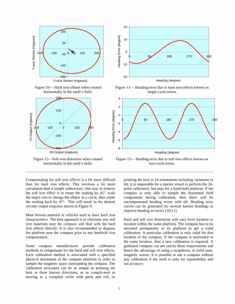
Nearby Ferrous Materials—Another consideration forheading accuracy is the effects of nearby ferrous materialson the earth's magnetic field [9-11]. Since heading isbased on the direction of the earth's horizontal field(Xh,Yh), the magnetic sensor must be able to measure thisfield without influence from other nearby magneticsources or disturbances. The amount of disturbancedepends on the material content of the platform andconnectors as well as ferrous objects moving near thecompass.

When a ferrous object is placed in a uniform magneticfield it will create disturbances as shown in Figure 8. Thisobject could be a steel bolt or bracket near the compass oran iron door latch close to the compass. The net result is acharacteristic distortion, or anomaly, to the earth’smagnetic field that is unique to the shape of the object.

Before looking at the effects of nearby magneticdisturbances, it is beneficial to observe an ideal outputcurve with no disturbances. When a two-axis (X,Y)magnetic sensor is rotated in the horizontal plane, theoutput plot of Xh vs. Yh will form a circle centered at the(0,0) origin (see Figure 9). If a heading is calculated ateach point on the circle, the result will be a linear sweepfrom 0° to 360°.

Ferrous Object + Uniform Magnetic Field = FieldDisturbance

Figure 8–Ferrous object disturbance in uniform field.

-200

-100

0

100

200

-200 -100 0 100 200

Xh Magnetic Field (mgauss)

Yh

Mag

netic

Fie

ld (

mga

uss)

Figure 9—Magnetic sensor outputs (X,Y) rotatedhorizontally in the earth’s field with no disturbances.

The effect of a magnetic disturbance on the heading willbe to distort the circle shown in Figure 9. Magneticdistortions can be categorized as two types—hard iron andsoft iron effects. Hard iron distortions arise frompermanent magnets and magnetized iron or steel on thecompass platform. These distortions will remain constantand in a fixed location relative to the compass for allheading orientations. Hard iron effects add a constantmagnitude field component along each axes of the sensoroutput. This appears as a shift in the origin of the circleequal to the hard iron disturbance in the Xh and Yh axis(see Figure 10). The effect of the hard iron distortion onthe heading is a one-cycle error and is shown in Figure 11.

To compensate for hard iron distortion, the offset in thecenter of the circle must be determined. This is usuallydone by rotating the compass and platform in a circle andmeasure enough points on the circle to determine thisoffset. Once found, the (X,Y) offset can be stored inmemory and subtracted from every reading. The net resultwill be to eliminate the hard iron disturbance from theheading calculation; as if it were not present[1].

The soft iron distortion arises from the interaction of theearth’s magnetic field and any magnetically soft materialsurrounding the compass. Like the hard iron materials, thesoft metals also distort the earth’s magnetic field lines.The difference is the amount of distortion from the softiron depends on the compass orientation. Soft ironinfluence on the field values measured by X and Y sensorsare depicted in Figure 12. Figure 13 illustrates thecompass heading errors associated with this effect—alsoknown as a two cycle error.

6

-250

-150

-50

50

150

-200 -100 0 100 200

Y-a

xis

Sen

sor

(mga

uss)

X-axis Sensor (mgauss)-20

-10

0

10

20

0 90 180 270 360

Hea

ding

Err

or (

degr

ee)

Heading (degree)

Figure 10— Hard iron offsets when rotatedhorizontally in the earth’s field.

Figure 11— Heading error due to hard iron effects known assingle-cycle errors.

-200

-100

0

100

200

-200 -100 0 100 200

Yh

Out

put (

mga

uss)

Xh Output (mgauss)-8

-6

-4

-2

0

2

4

0 90 180 270 360

Hea

ding

Err

or (

degr

ee)

Heading (degree)

Figure 12—Soft iron distortion when rotatedhorizontally in the earth’s field.

Figure 13— Heading error due to soft iron effects known astwo-cycle errors.

Compensating for soft iron effects is a bit more difficultthan for hard iron effects. This involves a bit morecalculation than a simple subtraction. One way to removethe soft iron effect is to rotate the reading by 45°, scalethe major axis to change the ellipse to a circle, then rotatethe reading back by 45°. This will result in the desiredcircular output response shown in Figure 9.

Most ferrous material in vehicles tend to have hard ironcharacteristics. The best approach is to eliminate any softiron materials near the compass and deal with the hardiron effects directly. It is also recommended to degaussthe platform near the compass prior to any hard/soft ironcompensation.

Some compass manufacturers provide calibrationmethods to compensate for the hard and soft iron effects.Each calibration method is associated with a specifiedphysical movement of the compass platform in order tosample the magnetic space surrounding the compass. Thecalibration procedure can be as simple as pointing thehost in three known directions, or as complicated asmoving in a complete circle with pitch and roll, or

pointing the host in 24 orientations including variations intilt. It is impossible for a marine vessel to perform the 24-point calibration, but easy for a hand-held platform. If thecompass is only able to sample the horizontal fieldcomponents during calibration, then there will beuncompensated heading errors with tilt. Heading errorcurves can be generated for several known headings toimprove heading accuracy [10,11].

Hard and soft iron distortions will vary from location tolocation within the same platform. The compass has to bemounted permanently to its platform to get a validcalibration. A particular calibration is only valid for thatlocation of the compass. If the compass is reoriented inthe same location, then a new calibration is required. Agimbaled compass can not satisfy these requirements andhence the advantage of using a strapdown, or solid state,magnetic sensor. It is possible to use a compass withoutany calibration if the need is only for repeatability andnot accuracy.

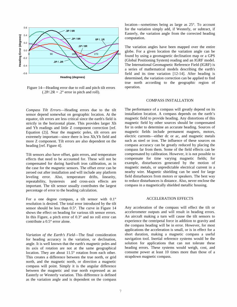
7

-0.6

-0.4

-0.2

0.0

0.2

0.4

0.6

0 90 180 270 360

Heading (degrees)

Hea

din

g E

rro

r (d

egre

es)

.1P / 0R

.2P / 0R

.3P / 0R

.2P / .2R

0P / .1R

Figure 14—Heading error due to roll and pitch tilt errors(.2P/.2R = .2° error in pitch and roll).

Compass Tilt Errors—Heading errors due to the tiltsensor depend somewhat on geographic location. At theequator, tilt errors are less critical since the earth's field isstrictly in the horizontal plane. This provides larger Xhand Yh readings and little Z component correction [ref.Equation (2)]. Near the magnetic poles, tilt errors areextremely important—since there is less Xh,Yh field andmore Z component. Tilt errors are also dependent on theheading [ref. Figure 4].

Tilt sensors also have offset, gain errors, and temperatureeffects that need to be accounted for. These will not becompensated for during hard/soft iron calibration, as inthe case for the magnetic sensors. The offset error can bezeroed out after installation and will include any platformleveling error. Also, temperature drifts, linearity,repeatability, hysteresis and cross-axis effects areimportant. The tilt sensor usually contributes the largestpercentage of error to the heading calculation.

For a one degree compass, a tilt sensor with 0.1°resolution is desired. The total error introduced by the tiltsensor should be less than 0.5°. The curve in Figure 14shows the effect on heading for various tilt sensor errors.In this Figure, a pitch error of 0.3° and no roll error cancontribute a 0.5° error alone.

Variation of the Earth’s Field—The final considerationfor heading accuracy is the variation, or declination,angle. It is well known that the earth's magnetic poles andits axis of rotation are not at the same geographicallocation. They are about 11.5° rotation from each other.This creates a difference between the true north, or gridnorth, and the magnetic north, or direction a magneticcompass will point. Simply it is the angular differencebetween the magnetic and true north expressed as anEasterly or Westerly variation. This difference is definedas the variation angle and is dependent on the compass

location—sometimes being as large as 25°. To accountfor the variation simply add, if Westerly, or subtract, ifEasterly, the variation angle from the corrected headingcomputation.

The variation angles have been mapped over the entireglobe. For a given location the variation angle can befound by using a geomagnetic declination map or a GPS(Global Positioning System) reading and an IGRF model.The International Geomagnetic Reference Field (IGRF) isa series of mathematical models describing the earth'sfield and its time variation [12-14]. After heading isdetermined, the variation correction can be applied to findtrue north according to the geographic region ofoperation.

COMPASS INSTALLATION

The performance of a compass will greatly depend on itsinstallation location. A compass depends on the earth’smagnetic field to provide heading. Any distortions of thismagnetic field by other sources should be compensatedfor in order to determine an accurate heading. Sources ofmagnetic fields include permanent magnets, motors,electric currents—either dc or ac, and magnetic metalssuch as steel or iron. The influence of these sources oncompass accuracy can be greatly reduced by placing thecompass far from them. Some of the field effects can becompensated by calibration. However, it is not possible tocompensate for time varying magnetic fields; forexample, disturbances generated by the motion ofmagnetic metals, or unpredictable electrical current in anearby wire. Magnetic shielding can be used for largefield disturbances from motors or speakers. The best wayto reduce disturbances is distance. Also, never enclose thecompass in a magnetically shielded metallic housing.

ACCELERATION EFFECTS

Any acceleration of the compass will effect the tilt oraccelerometer outputs and will result in heading errors.An aircraft making a turn will cause the tilt sensors toexperience the centripetal force in addition to gravity andthe compass heading will be in error. However, for mostapplications the acceleration is small, or is in effect for ashort duration, making a magnetic compass a usefulnavigation tool. Inertial reference systems would be thesolution for applications that can not tolerate theseheading errors. These systems would weigh, cost, andconsume power at least 10 times more than those of astrapdown magnetic compass.

8

CONCLUSION

A low cost compass has been discussed here having a onedegree accuracy requirement. At the heart of the compassis a three-axis MR magnetic sensor and a two-axiselectrolytic tilt sensor. Other circuits include a 12 to 14bit A/D converter, signal conditioning electronics and amicroprocessor. The error budget for heading accuracybreaks down as:

Magnetic sensor error 0.14°Temperature effects 0.29°Signal conditioning 0.05°Tilt sensor error 0.50°

Total Error 0.98°

The effects of nearby magnetic distortions can becalibrated out of the compass readings once it is securedto the platform. Caution must be taken in finding acompass location that is not too near varying magneticdisturbances and soft iron materials. Shielding effectsfrom speakers and high current conductors near thecompass may be necessary.

Variations in the earth's field from a true north headingcan be accounted for if the geographical location of thecompass is known. This can be achieved by using a mapmarked with the deviation angles to find the correctheading offset variation; or use a GPS system and theIGRF reference model to compute the variation angle.

Low cost compasses of the type described here aresusceptible to temporary heading errors duringaccelerations and banked turns. The heading accuracywill be restored once these accelerations diminish. With astrapdown compass there is no accuracy drift to worryabout since the heading is based on the true earth'smagnetic field. They tend to be very rugged to shock andvibration effects and consume very low power and aresmall in size.

REFERENCES

[1] M.J. Caruso, “Application of MagnetoresistiveSensors in Navigation Systems”, Sensors and Actuators1997, SAE SP-1220, (Feb. 1997) 15-21.

[2] M. Horton, C. Kitchin, “A Dual Axis Tilt SensorBased on Micromachined Accelerometers”, Sensors,(April 1996).

[3] Olson, Gregory J., et al, “Nongimbaled Solid-StateCompass”, Solid-State Sensor and Actuator Workshop,June, 1994.

[4] B.B. Pant, “Magnetoresistive Sensors”, ScientificHoneyweller, vol. 8, no.1, (Fall 1987) 29-34.

[5] J.E. Lenz, G.F.Rouse, L.K. Strandjord, B.B.Pant,A.Metze, H.B.French, E.T.Benser, D.R.Krahn, “A HighlySensitive Magnetoresistive Sensors”, Solid State Sensorsand Actuator Workshop, 1992.

[6] J.Goetz, T.Bratland, M.Caruso, “Designing withMagnetoresistive Sensors”, Sensor Expo Workshop,Philadelphia, October, 1996.

[7] Sensor Products Data Sheet, "1 and 2 AxisMagnetoresistive Microcircuits", Honeywell SSEC, 5/99,<www.magneticsensors.com>.

[8] M.J.Caruso, T.Bratland, C.H.Smith, R.Schneider, “ANew Perspective on Magnetic Field Sensing”, SensorsExpo Proceedings, October 1998, 195-213.

[9] M.J.Caruso, L.S. Withanawasam, “Vehicle Detectionand Compass Applications using AMR MagneticSensors”, Sensors Expo Proceedings, May 1999, 477-489.

[10] C.A. Lund, Compasses in Small Craft", Glasgow,Scotland: Brown, Son & Ferguson, Ltd., 1983, 39-62.

[11] W. Denne, Magnetic Compass Deviation andCorrection, Glasgow, Scotland: Brown, Son & Ferguson,Ltd., 1998.

[12] Y. Zhao, Vehicle Location and Navigation Systems,Norwood, MA: Artech House, Inc, 1997, Chapter 3.

[13] National Geomagnetic Information Center, websiteURL http://geomag.usgs.gov/

[14] National Geophysical Data Center, website URLhttp://www.ngdc.noaa.gov/

Unit conversion from SI to Gaussian: 79.6 A/m = 1 oersted 1 gauss = 1 oersted (in free air) 1 gauss = 10-4 tesla = 105 gamma 1 nanotesla = 10 microgauss = 1 gamma