Embed Size (px)
Citation preview
INFORMATICA, 2017, Vol. 28, No. 2, 303–328 303 2017 Vilnius University
DOI: http://dx.doi.org/10.15388/Informatica.2017.131
Holo-Entropy Based Categorical Data Hierarchical
Clustering
Haojun SUN1∗, Rongbo CHEN1, Yong QIN2, Shengrui WANG3
1Department of Computer Science, Shantou University, Shantou, China2State Key Laboratory of Rail Traffic Control and Safety, Beijing Jiaotong University
Beijing, China3Department of Computer Science, University of Sherbrooke, Sherbrooke, QC, Canada
e-mail: [email protected], [email protected], [email protected],
Received: January 2016; accepted: May 2017
Abstract. Clustering high-dimensional data is a challenging task in data mining, and clustering
high-dimensional categorical data is even more challenging because it is more difficult to mea-
sure the similarity between categorical objects. Most algorithms assume feature independence when
computing similarity between data objects, or make use of computationally demanding techniques
such as PCA for numerical data. Hierarchical clustering algorithms are often based on similar-
ity measures computed on a common feature space, which is not effective when clustering high-
dimensional data. Subspace clustering algorithms discover feature subspaces for clusters, but are
mostly partition-based; i.e. they do not produce a hierarchical structure of clusters. In this paper,
we propose a hierarchical algorithm for clustering high-dimensional categorical data, based on a re-
cently proposed information-theoretical concept named holo-entropy. The algorithm proposes new
ways of exploring entropy, holo-entropy and attribute weighting in order to determine the feature
subspace of a cluster and to merge clusters even though their feature subspaces differ. The algorithm
is tested on UCI datasets, and compared with several state-of-the-art algorithms. Experimental re-
sults show that the proposed algorithm yields higher efficiency and accuracy than the competing
algorithms and allows higher reproducibility.
Key words: hierarchical clustering, holo-entropy, subspace, categorical data.
1. Introduction and Problem Statement
The aim of clustering analysis is to group objects so that those within a cluster are
much more similar than those in different clusters. Clustering has been studied exten-
sively in the statistics, data-mining and database communities, and numerous algorithms
have been proposed (Schwenkera and Trentin, 2014; Sabit et al., 2011; Yu et al., 2012;
Fukunaga, 2013; Cover and Hart, 1967; Derrac et al., 2012; Santos et al., 2013). It has
been widely used for data analysis in many fields, including anthropology, biology, eco-
nomics, marketing, and medicine. Typical applications include disease classification, doc-
*Corresponding author.
304 H. Sun et al.
ument retrieval, image processing, market segmentation, scene analysis, and web ac-
cess pattern analysis (Guan et al., 2013; Li et al., 2013; Shrivastava and Tyagi, 2014;
Hruschka et al., 2006; Li et al., 2006; Lingras et al., 2005; Choi et al., 2012).
Hierarchical techniques are often used in cluster analysis. They aim to establish a hier-
archy of partition structure, using either bottom-upor top-down approaches. In the bottom-
up approach, at initialization, each object is represented by a single cluster. Clusters are
then successively merged based on their similarities until all the objects are grouped into
a single cluster, or until some special stopping conditions are satisfied. In the top-down
approach, on the other hand, larger clusters are successively divided to generate smaller
and more compact clusters until some stopping conditions are satisfied or each cluster
contains a single object. Traditionally, in the bottom-up approach, the pairwise similar-
ity (or distance) employed for merging clusters is often calculated on a common feature
space. Feature relevance or feature selection is addressed prior to the clustering process.
In this research, we will investigate feature relevance with respect to individual clusters
and cluster merging where each cluster may have its own relevant features. This is a very
important issue in hierarchical clustering of high-dimensional data. In this paper the terms
‘feature’, ‘attribute’ and sometimes ‘dimension’ are used interchangeably.
Automatically determining the relevancy of attributes in a categorical cluster will
be investigated in this paper. Conventional similarity measures, defined on the whole
feature space with the assumption that features are of equal importance, are not suit-
able for clustering high-dimensional data in many cases. In real-world applications, dif-
ferent clusters may lie in different feature subspaces with different dimensions. This
means the significance or relevance of an attribute is not the same to different clus-
ters. A cluster might be related to only a few dimensions (most relevant dimensions)
while the other dimensions (unimportant dimensions) contain random values. Attribute
weighting is employed to deal with these issues, but most weighting methods have been
designed solely for numeric data clustering (Huang et al., 2005; Lu et al., 2011). For
categorical data, the main difficulty is estimating the attribute weights based on the
statistics of categories in a cluster. In fact, in the existing methods (Bai et al., 2011a;
Xiong et al., 2011), an attribute is weighted solely according to the mode category for
that attribute. Consequently, the weights easily yield a biased indication of the relevance
of attributes to clusters. To solve this problem, it is necessary to analyse the relationship
between attributes and clusters.
In this paper, we propose a novel algorithm named Hierarchical Projected Clustering
for Categorical Data (HPCCD). The HPCCD algorithm has been designed to deal with
three main issues. The first is analysing attribute relevance based on the holo-entropy the-
ory (Wu and Wang, 2013). The holo-entropy is defined as the sum of the entropy and the
total correlation of the random vector, and can be expressed by the sum of the entropies
on all attributes. It will be used to analyse the relationship between attributes and clus-
ter structure. The second issue is how to decide to merge two clusters in the absence of
an effective pairwise similarity measure. The problem arises due to the fact that different
subclusters may have their own relevant subspaces. And finally, the third issue is find-
ing the projected clusters based on the intra-class compactness. Our algorithm has two
Holo-Entropy Based Categorical Data Hierarchical Clustering 305
phases, based on the conventional steps in agglomerative clustering. The first is to divide
the dataset into Kinit (the initial number of clusters) subclusters in an initialization step.
And the second is to iteratively merge these small clusters to yield larger ones, until all the
objects are grouped in one cluster or a desired number of clusters. Experimental results
on nine UCI real-life datasets show that our algorithm performs effectively compared to
state-of-the-art algorithms.
The rest of the paper is organized as follows: Section 2 is a brief review of related work.
In Section 3, we introduce the mutual information, total correlation, and holo-entropy
concepts used in the paper. Section 4 describes the details of our algorithm HPCCD, with
an illustrative example. In Section 5, we present experimental results, in comparison with
other state-of-the-art algorithms. Finally, we conclude our paper and suggest future work
in Section 6.
2. Related Work
In this section, we briefly review major existing works related to our research. Many
clustering algorithms for categorical data are based on the partition approach. The most
popular of these is Huangs K-modes algorithm (Huang, 1998), which is an extension of
the K-means paradigm to the categorical domain. It replaces the mean of a cluster by the
mode and updates the mode based on the maximal frequency of the value of each attribute
in a cluster. A number of partition-based algorithms have been developed based on the
K-modes approach. In Jollois and Nadif (2002), Jollois et al. develop the Classification
EM algorithm (CEM) to estimate the parameters of a mixture model based on the classi-
fication likelihood approach. In Gan et al. (2005), Gan et al. present a genetic K-modes
algorithm named GKMODE. It introduces a K-modes operator in place of the normal
crossover operator and finds a globally optimal partition of a given categorical dataset
into a specified number of clusters. Other extensions of the K-modes algorithm include
fuzzy centroids (Kim et al., 2004) using fuzzy logic, more effective initialization methods
(Cao et al., 2009; Bai et al., 2011b) for the K-modes and fuzzy K-modes, attribute weight-
ing (He et al., 2011) and the use of genetic programming techniques for fuzzy K-modes
(Gan et al., 2009).
Also proposed in addition to all the K-modes algorithms is k-ANMI (He et al.,
2005), a K-means-like clustering algorithm for categorical data that optimizes an ob-
jective function based on mutual information sharing. Most of the conventional al-
gorithms (Shrivastava and Tyagi, 2014; Hruschka et al., 2006; Xiong et al., 2011;
Wu and Wang, 2013) involve optimizing an objective function defined on a pairwise
measure of the similarity between objects. Unfortunately, this optimization problem is
usually NP-complete and requires the use of heuristic methods in practice. In such so-
lutions, the focus is primarily on the relationship between objects and clusters, while at-
tribute relevance within a cluster is often ignored (Barbar et al., 2002; Qin et al., 2014;
Ganti et al., 1999; Greenacre and Blasius, 2006). Moreover, the lack of an intuitive method
for determining the number of clusters and high time complexity are common challenges
for this type of algorithm.
306 H. Sun et al.
Projected clustering is a major technique for high-dimensional data clustering, whose
aim is to discover the clusters and their relevant attributes simultaneously. A projected
cluster is defined by both its data points and the relevant attributes (Bouguessa and Wang,
2009; Domeniconi et al., 2004; Parsons et al., 2004) forming its feature subspace. For
example, HARP (Yip et al., 2004) is a hierarchical projected clustering algorithm based
on the assumption that two data points are likely to belong to the same cluster if they are
very similar to each other along many dimensions. However, when the number of relevant
dimensions per cluster is much lower than the dataset dimensionality, such an assumption
may not be valid, because relevant information concerning these data points in a large sub-
space is lost. Some projected clustering algorithms, such as PROCLUS (Aggarwal et al.,
1999) and ORCLUS (Aggarwal and Yu, 2002), require the user to provide the average di-
mensionality of the subspaces, which is very difficult to establish in real-life applications.
PCKA (Bouguessa and Wang, 2009), a distance-based projected clustering algorithm, was
recently proposed to improve the quality of clustering when the dimensionalities of the
clusters are much lower than that of the dataset. However, it requires users to provide val-
ues for some input parameters, such as the number of nearest neighbours of a 1D point,
which may significantly affect its performance. These algorithms are dependent on pair-
wise similarity measures which do not take into account correlations between attributes.
Many clustering algorithms based on the hierarchical technique have been proposed.
ROCK (Guha et al., 1999) is an agglomerative hierarchical clustering algorithm based
on the extension of the pairwise similarity measure. It extends the Jaccard coefficient
similarity measure by exploiting the concept of neighbourhood. Its performance depends
heavily on the neighbour threshold and the time complexity depends on the number of
neighbours. However, these parameters are difficult to estimate in real applications. In-
stead of using pairwise similarity measures, the K-modes algorithm (Guha et al., 1999;
Zhang and Fang, 2013) defines a similarity between an individual categorical object and
a set of categorical objects. When the clusters are well established, this approach has the
advantage of being more meaningful. The performance of the K-modes algorithms relies
heavily on the initialization of the K modes. DHCC (Xiong et al., 2011) proposes a divi-
sive hierarchical clustering algorithm in which a meaningful object-to-clusters similarity
measure is defined. DHCC is capable of discovering clusters embedded in subspaces, and
is parameter-free with linear time complexity. However, DHCCPs space complexity is
a limitation, as it depends on the square of the number of values of all the categorical
attributes.
Information theory is also frequently used in many clustering models (Yao et al., 2000;
Barbar et al., 2002). The goal of these approaches is to seek an optimum grouping of the
objects such that the entropy is the smallest. An entropy-based fuzzy clustering algorithm
(EFC) is proposed in Yao et al. (2000). EFC calculates entropy values and implements
clustering analysis based on the degree of similarity. It requires the setting of a similar-
ity threshold to control the similarity among the data points in a cluster. This parameter,
which affects the number of clusters and the clustering accuracy, is very difficult to de-
termine. The COOLCAT algorithm (Barbar et al., 2002) employs the notion of entropy
in assigning unclustered objects. A given data object is assigned to a cluster such that
Holo-Entropy Based Categorical Data Hierarchical Clustering 307
the entropy of the resulting clustering is minimal. The incremental assignment terminates
when every object has been placed in some cluster. The clustering quality depends heav-
ily on the input order of the data objects. The LIMBO algorithm (Andritsos et al., 2004)
is a hierarchical clustering algorithm based on the concept of an Information Bottleneck
(IB) which quantifies the relevant information preserved in clustering results. It proposes
a novel measurement for the similarity among subclusters by way of the Jensen–Shannon
divergence.
Finally, the MGR algorithm (Qin et al., 2014) searches equivalence classes from at-
tribute partitions to form the clustering of objects which can share the greatest possible
quantity of information with the attribute partitions. First, MGR selects the clustering at-
tribute whose partition shares the most information with the partitions defined by other
attributes. Then, on the clustering attribute, the equivalence class with the highest intra-
class similarity is output as a cluster, and the rest of the objects form the new current
dataset. The above two steps are repeated on the new current dataset until all objects are
output. In MGR, because the attributes are selected one by one, the relevancy of attributes
(or combinations of attributes) is not considered sufficiently. For example, say attribute
A1 has the most information, and A2 is in second place. It is not necessarily true that the
combination A1, A2 has more information than some other combination A3, A4. How to
select the subcluster of attributes which shares the most information with the partitions
will be analysed in this paper.
3. The Holo-Entropy Theory
In this section, we provide a brief description of information entropy, and give a more
detailed explanation of the concepts of mutual information, total correlation and holo-
entropy (Wu and Wang, 2013) used by the algorithm proposed in this paper.
Entropy is a measure of the uncertainty of a system state. As formulated in information
theory (Shannon, 1948), the concept is often used to measure the degree of disorder or
chaos of a dataset, or to describe the uncertainty of a random variable. For a given discrete
random variable S = (s1, s2, . . . , sm), let the corresponding probability of appearance be
{p(s1),p(s2), . . . , p(sm)}, where p(si) satisfies∑m
i=1p(si) = 1. The entropy of S is de-
fined as E(S) = −∑m
i=1p(si ) ln(p(si)). The entropy allows to assess the structure of an
attribute, i.e. whether its values are distributed compactly or sparsely. Therefore, it can be
used as a criterion on an attribute that expresses the degree to which an attribute is or is
not characteristic for a cluster.
Many high-dimensional data clustering approaches are based on the attribute indepen-
dence hypothesis (Barbar et al., 2002; Ganti et al., 1999; Greenacre and Blasius, 2006).
Such a hypothesis not only ignores the degree of correlation among attributes, but also
fails to consider attribute relevance and heterogeneity in the data. Methods derived from
these approaches do not satisfy the requirements of many practical applications. The holo-
entropy (Wu and Wang, 2013) is a compactness measure that incorporates not only the
distribution of individual attributes but also correlations between attributes. It has been
effectively used in evaluating the likelihood of a data object being an outlier. There is as
308 H. Sun et al.
yet no reported work on how holo-entropy can contribute to high-dimensional categorical
data clustering. Our hypothesis in this work is that the holo-entropy may contribute to
relevant subspace detection and compactness measurement in cluster analysis. Actually,
the goal of subspace detection is to find a set of attributes on which the data of a cluster
are distributed compactly. This attribute set expresses the features of the cluster.
In this paper, we develop a new method that utilizes the holo-entropy for hierarchical
clustering. Based on the analysis of the intrinsic relevance of features and objects in sub-
clusters, we develop a principled approach for selecting clusters to merge and determining
the feature subspace of the merged cluster. The holo-entropy is used to measure the intrin-
sic relevance. The main idea is that the holo-entropy of two subclusters originating from
the same class should be much smaller than if the two subclusters originate from different
classes. Therefore, the two subclusters with minimal holo-entropy are selected to merge
in the hierarchical clustering. In order to describe our algorithm, the following notation
and definitions are introduced.
We use X = {x1, x2, . . . , xn} to represent the dataset with n samples, where each xi
has m categorical attributes. The m attributes [A1,A2, . . . ,Am]T are also repre-
sented by the attribute vector A. Each attribute Ai has a value domain defined by
[ai,1, ai,2, . . . , ai,ni ] (1 6 i 6 m), where ni is the number of distinct values in attribute Ai .
From the information-theoretic perspective, Ai is considered a random variable, and
A = [A1,A2,A3, . . . ,Am]T is considered a random vector. The entropy E(A) of the ran-
dom vector A on the set X is defined, according to the chain rule for the entropy (Cover
and Thomas, 2012), by:
E(A) = E(A1,A2, . . . ,Am) =
m∑
i=1
E(Ai | Ai−1, . . . ,A1)
= E(A1) + H(A2 | A1) + · · · + E(Am | Am−1, . . . ,A1) (1)
where E(Ai | Ai−1, . . . ,A1) = −∑
Ai ,Ai−1,...,A1p(Ai,Ai−1, . . . ,A1) lnp(Ai | Ai−1,
. . . ,A1) and the probability functions p() are estimated from X.
Definition 1 (Mutual information). The mutual information (He et al., 2005; Srinivasa,
2005) of random variables A1 and A2 is:
I (A1,A2) =∑
A1;A2
p(A1,A2) lnp(A1 | A2)
p(A1) ∗ p(A2)= E(A1) − E(A1 | A2). (2)
Definition 2 (Conditional mutual information). The conditional mutual information
(Watanabe, 1960; Filippone and Sanguinetti, 2010) between two random variables A1
and A2 on condition of A3 is:
I (A1,A2 | A3) = H(A1 | A3) − H(A1 | A2,A3). (3)
Holo-Entropy Based Categorical Data Hierarchical Clustering 309
Table 1
The example of Dataset1.
No. object A1 A2 A3 Label
1 0 1 0 C1
2 0 2 2 C1
3 0 2 1 C1
4 0 2 1 C1
5 2 3 2 C2
6 2 3 3 C2
7 1 3 0 C2
8 0 3 3 C2
Definition 3 (Total correlation). According to Watanabe’s proof (Watanabe, 1960) that
total correlation C(Y ) on the set X is equal to the sum of all mutual information among
random variables:
C(A) =
m∑
i=1
E(Ai) − E(A) (4)
where
C(A) =
m∑
i=2
∑
{r1,r2,...,ri}∈{1,2,...,m}
I (Ar1, . . . ,Ari )
=∑
{r1,r2,...,ri}∈{1,2,...,m}
I (Ar1,Ar2
) + · · · + I (Ar1, . . . ,Ari ),
r1, r2, . . . , ri are attribute numbers varying from 1 to m, I (Ar1, . . . ,Ari ) = I (Ar1
, . . . ,
Ari−1) − I (Ar1
, . . . ,Ari−1| Ari ) is the multivariate mutual information of Ar1
, . . . ,Ari ,
and I (Ar1, . . . ,Ari−1
| Ari ) = E(I (Ar1, . . . ,Ari−1
|Ari )) is the conditional mutual infor-
mation. Thus, the total correlation can be used for estimating the interrelationships among
the attributes or shared information of subclusters.
Based on Wu and Wang (2013), the definition of holo-entropy is as follows: The holo-
entropy HL(A) is defined as the sum of the entropy and the total correlation of the random
vector A, and can be expressed by the sum of the entropies on all attributes.
HL(A) = E(A) + C(A) =
m∑
i=1
E(Ai). (5)
Moreover, HL(A) = E(A) holds if and only if all the attributes are independent.
From what has been discussed above, the holo-entropy can be used to measure the com-
pactness of a dataset or a cluster more effectively, since it evaluates not only the disor-
der of the objects in the dataset but also correlation between variables. In fact, the val-
ues of HL() calculated on subsets of attributes and/or on subsets (groups) of data re-
veal cluster structures hidden in the data. As a simple example, let us look at a dataset
(Dataset1) shown in Table 1. Intuitively, this dataset has two classes (or clusters), one
310 H. Sun et al.
comprising objects {1,2,3,4} and the other objects {5,6,7,8}. We can also easily ob-
serve that the subspace {A1,A2} more strongly reflects an intrinsic cluster structure
with objects {1,2,3,4} than do other attribute combinations. Indeed, the holo-entropies
on the three non-single-dimensional subspaces are respectively HL(A1,A2) = 0.5623,
HL(A1,A3) = 1.0397, HL(A2,A3) = 1.6021 and HL(A1,A2,A3) = 1.6021. These in-
dicate clearly that {A1,A2} is the subspace of choice, given that the holo-entropy on
it is the smallest. On the other hand, if we calculate the holo-entropy on different data
subsets such as HL{1,2,3,4}(A1,A2,A3) = 1.6021, HL{3,4,5,6}(A1,A2,A3) = 2.0794,
HL{1,2,3,4,5,6}(A1,A2,A3) = 2.9776, we also observe that the subset {1,2,3,4} is clearly
a much better cluster candidate than other subsets.
From this example, we can see that the holo-entropy of two merged subclusters from
the same (homogeneous) class is much smaller than that of merged subclusters from differ-
ent (heterogeneous) classes. This indicates that holo-entropy is an effective measurement
for the compactness of a subspace in a cluster. In what follows, we will use the holo-entropy
for subspace detection. Moreover, we will employ the soft clustering method (Domeniconi
et al., 2004; Gan and Wu, 2004; Nemalhabib and Shiri, 2006) and the properties of holo-
entropy for merging subclusters in the hierarchical clustering.
4. HPCCD Algorithm
In this section, we present our Hierarchical Projected Clustering algorithm for Categorical
Data (HPCCD) in detail. To illustrate the ideas underlying the algorithm, we also provide
a working example with 11 objects from the dataset Soybean, as shown in Table 2. The
process of HPCCD draws on a conventional hierarchical clustering approach for its ma-
jor steps, including initially grouping the data into small clusters and iterating between
searching for the closest pair of subclusters and merging the pair. Our contribution is the
design of new methods based on holo-entropy for detecting the relevant subspace of each
subcluster and evaluating the structure compactness of a pair of subclusters in order to
select the most similar subclusters to merge. Our algorithm is described as follows:
Algorithm HPCCD
Input: Dataset X, threshold r and the terminal condition Kinit which is the
desired number of clusters;
Output: clusters of Dataset X.
Begin
Initialization (Grouping the data into subclusters C);
For each subcluster in set C
A: relevant subspace selection
A1: Detect the relevant subspace of each subcluster of C;
A2: Assign weights to the attributes in the relevant subspace;
B: compactness calculation (calculate compactness binding weight with
holo-entropy);
Holo-Entropy Based Categorical Data Hierarchical Clustering 311
Choose the most compact pair of subclusters to merge and update set C;
End
until satisfaction of the termination condition of K desired clusters.
The details of each step will be described in the following sub-sections.
4.1. Initialization
Cluster initialization in our approach is a necessary step as it makes it meaningful to use the
information-theoretic method to estimate attribute relevance and also reduces the number
of cluster merging steps. For the initialization of our agglomerative clustering algorithm,
the dataset is first divided into small subclusters. In order to ensure that objects in the
same subcluster are as similar as possible, we use the following categorical data similarity
measurement for initialization. The similarity between any two objects Xi and Xj can be
defined as follows:
sim(Xi,Xj ) =
∑md=1
‖ xid , xjd ‖
m, (6)
‖xid , xjd‖ =
{
1 xid = xjd ,
0 xid 6= xjd(7)
where m is the number of dimensions of object X and xid , xjd are the d th attribute values
of Xi , Xj , respectively. Drawing inspiration from Nemalhabib and Shiri (2006), we extend
this similarity measure to calculate the similarity between an object and a cluster. The
definition is as follows:
Sim(Xi,C) =
∑|C|a=1
∑md=1
‖xid , xad‖
|C| ∗ m(8)
where |C| is the size of cluster C, Xa is one of the objects in C and the first sum in the
numerator covers all the objects in C. The main phase of initialization is described as
follows:
Initialization
Input: Dataset X = {x1, x2, . . . , xn}, threshold r
Output: Kinit subclusters C = {C1,C2, . . . ,CKinit }.
Begin
Set x1 ∈ C1 and R = X − {x1}, k = 1;
For each xi in R
Use Eq. (8) to calculate similarities S1, . . . , Sk of xi to each of
the clusters {C1,C2, . . . ,Ck};
If Sl = max{S1, . . . , Sk} > r;
Allocate xi to Cl ;
312 H. Sun et al.
Table 2
11 samples from the Soybean dataset.
No. Clusters A1 A2 A3 A4 A5 Class
object label
1 C1 0 1 1 0 1 1
2 C1 0 1 2 1 1 1
3 C1 0 1 1 1 1 1
4 C1 0 1 2 0 1 1
5 C2 0 1 0 2 2 1
6 C2 0 1 1 0 2 1
7 C2 0 1 0 2 2 1
8 C3 1 0 1 4 0 2
9 C3 0 0 1 4 0 2
10 C3 0 0 1 4 0 2
11 C3 1 1 1 4 0 2
Else
k = k + 1;
Allocate xi to Ck ;
End if
End for
Kinit = k
End
In this algorithm, Eq. (8) is used to calculate the similarities S1, . . . , Sk of xi to each
of C1 to Ck . If at least one of these similarities is larger than r , then xi is assigned to an
existing cluster; otherwise, a new cluster Ck+1 will be created. The final number of initial
clusters is thus controlled by the similarity threshold r , which ranges in (0,1). In fact, the
larger r will result in more sub-clusters with less objects, on the other hand, the small r
results in less sub-clusters with more objects. In theory, the choice of r is application
dependent, however, we found from our experiments that the results are not sensitive to
the choice of r as long as its value is large enough to ensure creation of a sufficient number
of initial clusters. Our guideline is that if the attribute values of an object are the same as
those of a sub-cluster at about three quarters of the dimensions or more, the object can
be regarded as coming from the same sub-cluster. To ensure that all the objects in each
cluster are sufficiently similar to each other, we recommend choosing r between 0.7 and
0.95. In our experiments, we have chosen r to be 0.80 for different datasets.
The similarity measure of Eq. (8) coupled with a high similarity threshold r makes the
initialization procedure significantly less sensitive to the input order. This is very impor-
tant for the hierarchical clustering proposed in this paper, as the final result depends on
the initial clusters. An example is shown in Table 2 in which three clusters can be consid-
ered to reside in the two-class dataset with 11 objects. Objects 1 to 7 from class 1 form
two clusters: objects 1 to 4 as one cluster and 5 to 7 as another. The rest of the objects,
8 to 11 from class 2, form the third cluster. Each object is represented by five attributes
A1 to A5, and the corresponding class number is given in the Label column. Remark that
Holo-Entropy Based Categorical Data Hierarchical Clustering 313
significant differences exist between data objects belonging to the same cluster. After the
initialization phase, the dataset will be divided into three subclusters C1, C2 and C3, us-
ing Eqs. (6), (7), (8): objects 1 to 4, 5 to 7 and 8 to 11 are assigned to subclusters C1,C2
and C3, respectively. Such a result is obtained regardless of the order in which the data
objects are presented to the initialization procedure.
4.2. Relevant Subspace Selection
In this subsection, we address the problem of optimally determining the subspace
(Domeniconi et al., 2004; Gan and Wu, 2004) for a given cluster. The idea of our approach
is to optimally separate the attributes into two groups, of which one generates a subspace
that pertains to the cluster. In our method, the entropy is used for attribute evaluation and
holo-entropy is employed as the criterion for subspace detection.
Subspace clustering (Gan and Wu, 2004; Parsons et al., 2004) is extensively applied
for clustering high-dimensional data in the field because of the curse of dimensionality
(Parsons et al., 2004). In subspace clustering, finding the relevant subspaces in a cluster
is of great significance. Informally, a relevant or characteristic attribute of a cluster is an
attribute on which the data distribution is concentrated as compared to a non-characteristic
attribute of the cluster. Characteristic attributes of a cluster form the relevant subspace of
the cluster. Generally, different clusters have different characteristic subspaces. The non-
characteristic or noise attributes are distributed in a diffuse way; i.e. data should be sparse
in the subspace generated by noise attributes. We also call these attributes irrelevant w.r.t.
the cluster structure. How to separate the attribute space into relevant and noise subspaces
is a key issue in subspace clustering.
In order to determine the relevant attributes for each cluster, we need to find an optimal
division that separates characteristic attributes from noise ones. Although there has been a
great deal of work reported on subspace clustering, attribute relevance analysis in the exist-
ing approaches is often based on analysing the variance of each individual attribute while
assuming that attributes are mutually independent (Barbar et al., 2002; Ganti et al., 1999;
Greenacre and Blasius, 2006). Moreover, existing entropy-based algorithms such as Bar-
bar et al. (2002), Qin et al. (2014) usually use ad-hoc values of parameters to determine
the separation between relevant and non relevant attributes, and such methods lack flexi-
bility for practical applications. The proposed strategy makes use of the holo-entropy in
Eq. (5), as it provides an efficient and effective way to estimate the quality of cluster struc-
ture of a given data subset on a given set of attributes. It establishes the separation based
on an automatic process.
Let the whole feature space of a cluster (or cluster candidate) D be Q, and let Q
be separated into two feature subspaces S and N , where S is a candidate for the relevant
subspace of D and N is a candidate for its non-relevant subspace, Q = N ∪S and (N ∩S =
∅). We want to evaluate the quality of the feature-space separation in order to find an
optimal S as the relevant subspace of D. In fact, by using holo-entropy, the quality of
314 H. Sun et al.
the feature subspace S can be evaluated by HL(D|S). This measure can be equivalently
written as
qcs(D|S) =∑
i∈S
std(i) (9)
and
std(i) =entropy(i) − min
max− min(10)
where entropy(i), min and max respectively denote the entropy of attribute Ai and the
minimum and maximum values of attribute entropy in the whole space of a subcluster.
std(i) refers to the normalized information entropy of attribute Ai . An advantage of using
normalized entropies is that it allows another seemingly close function to be defined to
evaluate the quality of N as a non-relevant subspace.
qncs(D|N) =∑
i∈N
(
1 − std(i))
. (11)
In both cases, the smaller the value of qcs() (or qncs()), the better the quality of S
(or N ) as a (non-)relevant subspace. From these two functions, we define a new measure
for evaluating the quality of the feature-space separation by
AF(D,Q) =qcs(D|S)
nb_dims(S)+
qncs(D|N)
nb_dims(N). (12)
Obviously, this measure is designed to strike a balance between the sizes of the relevant
and non-relevant subspaces.
The optimization (minimization, in fact) of Eq. (12) aims to find S that leads to the
optimal value of AF(D,Q). This optimization can be performed by a demarcation detec-
tion process. In fact, if we first sort all the dimensions in increasing order of entropies; i.e.
supposing that for any pair of dimensions i and j , we have entropy(i), entropy(j), then the
optimization of (12) consists in finding a demarcation point e such that the S composed of
dimensions from 1 to e (and entropy from e + 1 to m) minimizes AF(D,Q). In this opti-
mization, we use in Eq. (12) the average of the holo-entropy measures in Eqs. (9) and (11)
to compute the demarcation point. This choice is made to favour a balanced separation.
For the Soybean dataset, after initialization, the dataset is divided into three subclusters
C1, C2, and C3. Based on the information entropy, Eq. (10) is used for normalization,
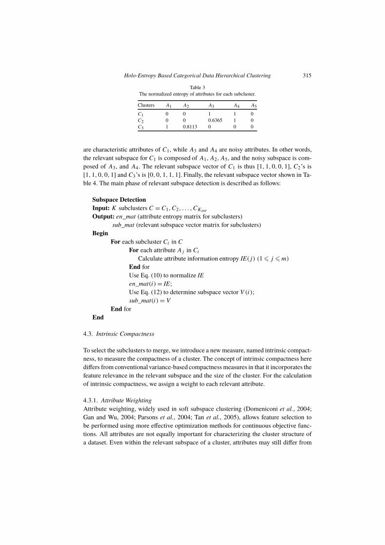
and the normalized entropy of each attribute of each subcluster is shown in Table 3. The
values in Table 3 are the related normalized entropy of the corresponding attribute of each
subcluster. For instance, the value of 0.8113 is the standard information entropy of C3’s
attribute A2.
The optimization in Eq. (12) allows us to determine the relevant subspace for each sub-
cluster. The results are shown in Table 4, where y indicates that the corresponding attribute
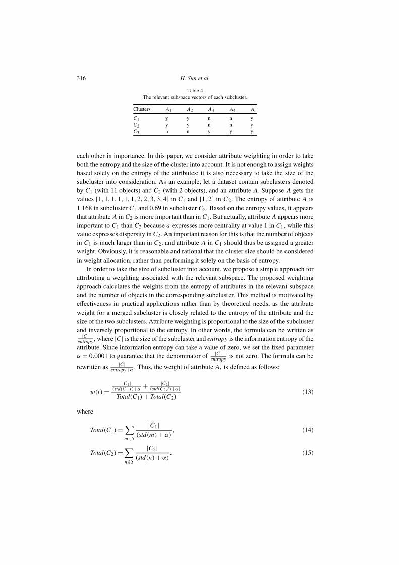
is a characteristic attribute while n indicates a noisy attribute. For instance, A1,A2,A5
Holo-Entropy Based Categorical Data Hierarchical Clustering 315
Table 3
The normalized entropy of attributes for each subcluster.
Clusters A1 A2 A3 A4 A5
C1 0 0 1 1 0
C2 0 0 0.6365 1 0
C3 1 0.8113 0 0 0
are characteristic attributes of C1, while A3 and A4 are noisy attributes. In other words,
the relevant subspace for C1 is composed of A1,A2,A5, and the noisy subspace is com-
posed of A3, and A4. The relevant subspace vector of C1 is thus [1,1,0,0,1], C2’s is
[1,1,0,0,1] and C3’s is [0,0,1,1,1]. Finally, the relevant subspace vector shown in Ta-
ble 4. The main phase of relevant subspace detection is described as follows:
Subspace Detection
Input: K subclusters C = C1,C2, . . . ,CKinit
Output: en_mat (attribute entropy matrix for subclusters)
sub_mat (relevant subspace vector matrix for subclusters)
Begin
For each subcluster Ci in C
For each attribute Aj in Ci
Calculate attribute information entropy IE(j) (1 6 j 6 m)
End for
Use Eq. (10) to normalize IE
en_mat(i) = IE;
Use Eq. (12) to determine subspace vector V (i);
sub_mat(i) = V
End for
End
4.3. Intrinsic Compactness
To select the subclusters to merge, we introduce a new measure, named intrinsic compact-
ness, to measure the compactness of a cluster. The concept of intrinsic compactness here
differs from conventional variance-based compactness measures in that it incorporates the
feature relevance in the relevant subspace and the size of the cluster. For the calculation
of intrinsic compactness, we assign a weight to each relevant attribute.
4.3.1. Attribute Weighting
Attribute weighting, widely used in soft subspace clustering (Domeniconi et al., 2004;
Gan and Wu, 2004; Parsons et al., 2004; Tan et al., 2005), allows feature selection to
be performed using more effective optimization methods for continuous objective func-
tions. All attributes are not equally important for characterizing the cluster structure of
a dataset. Even within the relevant subspace of a cluster, attributes may still differ from
316 H. Sun et al.
Table 4
The relevant subspace vectors of each subcluster.
Clusters A1 A2 A3 A4 A5
C1 y y n n y
C2 y y n n y
C3 n n y y y
each other in importance. In this paper, we consider attribute weighting in order to take
both the entropy and the size of the cluster into account. It is not enough to assign weights
based solely on the entropy of the attributes: it is also necessary to take the size of the
subcluster into consideration. As an example, let a dataset contain subclusters denoted
by C1 (with 11 objects) and C2 (with 2 objects), and an attribute A. Suppose A gets the
values [1,1,1,1,1,1,2,2,3,3,4] in C1 and [1,2] in C2. The entropy of attribute A is
1.168 in subcluster C1 and 0.69 in subcluster C2. Based on the entropy values, it appears
that attribute A in C2 is more important than in C1. But actually, attribute A appears more
important to C1 than C2 because a expresses more centrality at value 1 in C1, while this
value expresses dispersity in C2. An important reason for this is that the number of objects
in C1 is much larger than in C2, and attribute A in C1 should thus be assigned a greater
weight. Obviously, it is reasonable and rational that the cluster size should be considered
in weight allocation, rather than performing it solely on the basis of entropy.
In order to take the size of subcluster into account, we propose a simple approach for
attributing a weighting associated with the relevant subspace. The proposed weighting
approach calculates the weights from the entropy of attributes in the relevant subspace
and the number of objects in the corresponding subcluster. This method is motivated by
effectiveness in practical applications rather than by theoretical needs, as the attribute
weight for a merged subcluster is closely related to the entropy of the attribute and the
size of the two subclusters. Attribute weighting is proportional to the size of the subcluster
and inversely proportional to the entropy. In other words, the formula can be written as|C|
entropy, where |C| is the size of the subcluster and entropy is the information entropy of the
attribute. Since information entropy can take a value of zero, we set the fixed parameter
α = 0.0001 to guarantee that the denominator of|C|
entropyis not zero. The formula can be
rewritten as|C|
entropy+α. Thus, the weight of attribute Ai is defined as follows:
w(i) =
|C1|(std(C1,i)+α
+|C2|
(std(C2,i)+α)
Total(C1) + Total(C2)(13)
where
Total(C1) =∑
m∈S
|C1|
(std(m) + α), (14)
Total(C2) =∑
n∈S
|C2|
(std(n) + α). (15)
Holo-Entropy Based Categorical Data Hierarchical Clustering 317
Table 5
Relevant subspace vectors of merged subclusters.
Clusters A1 A2 A3 A4 A5
C1 ∪ C2 y y n n y
C1 ∪ C3 y y y y y
C2 ∪ C3 y y y y y
Table 6
Relevant subspace weights for each merged subcluster.
Clusters A1 A2 A3 A4 A5
C1 ∪ C2 0.3333 0.3333 * * 0.3333
C1 ∪ C3 0.1667 0.1667 0.1667 0.1667 0.3333
C2 ∪ C3 0.1429 0.1429 0.1905 0.1905 0.3333
Here w(i) refers to the weight of attribute Ai which is a member of the relevant subspace
of C1 ∪C2 , S is the union subspace of the two subclusters, |C1| and |C2| denote the respec-
tive sizes of subclusters C1 and C2, and std(C1, i) and std(C2, i) denote the normalized
entropies of subclusters C1 and C2, respectively.
With the above formulas, we consider both the attribute entropy and the size of the
subclusters in computing the weight of an attribute in a merged cluster. The initial impor-
tance of each attribute is modulated by the size of the subcluster. An important attribute
coming from a large subcluster is assigned a larger weight. On the other hand, an impor-
tant attribute coming from a small subcluster is assigned a proportionally smaller weight.
The contribution of the selected relevant subspace of each subcluster to the merged cluster
is thus better balanced.
Continuing with the example given in Section 4.2, the subspaces corresponding to the
merged subclusters are shown in Table 5. y indicates that the corresponding attribute is
a characteristic attribute while n indicates a noisy attribute. The relevant subspaces for
C1 and C2 are composed of [A1,A2,A5] and [A1,A2,A5], respectively. Choosing the
characteristic attribute union set, [A1,A2,A5] serves as the relevant subspace of C1,C2.
The relevant subspace weights for each merged subcluster, according to formulas (13),
(14) and (15), are given in Table 6 (∗ denotes that the attribute is a noise attribute for the
merged subcluster).
The main phase of weight calculation is described as follows:
Weight Calculation
Input: K subclusters C = {C1,C2, . . . ,CKinit }
en_mat (attribute entropy matrix for subclusters)
sub_mat (relevant subspace vector matrix for subclusters)
Output: w_mat (weight matrix for merged subclusters)
Begin
For each subcluster Ci in C
Calculate the size of Ci , |Ci |
318 H. Sun et al.
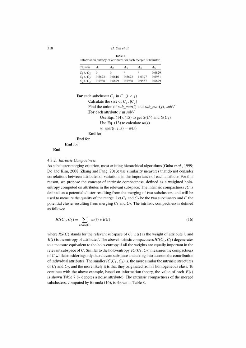
Table 7
Information entropy of attributes for each merged subcluster.
Clusters A1 A2 A3 A4 A5
C1 ∪ C2 0 0 * * 0.6829
C1 ∪ C3 0.5623 0.6616 0.5623 1.0397 0.6931
C2 ∪ C3 0.5938 0.6829 0.5938 0.9557 0.6829
For each subcluster Cj in C, (i < j)
Calculate the size of Cj , |Cj |
Find the union of sub_mat(i) and sub_mat(j), subV
For each attribute s in subV
Use Eqs. (14), (15) to get S(Ci) and S(Cj )
Use Eq. (13) to calculate w(s)
w_mat(i, j, s) = w(s)
End for
End for
End for
End
4.3.2. Intrinsic Compactness
As subcluster merging criterion, most existing hierarchical algorithms (Guha et al., 1999;
Do and Kim, 2008; Zhang and Fang, 2013) use similarity measures that do not consider
correlations between attributes or variations in the importance of each attribute. For this
reason, we propose the concept of intrinsic compactness, defined as a weighted holo-
entropy computed on attributes in the relevant subspace. The intrinsic compactness IC is
defined on a potential cluster resulting from the merging of two subclusters, and will be
used to measure the quality of the merge. Let C1 and C2 be the two subclusters and C the
potential cluster resulting from merging C1 and C2. The intrinsic compactness is defined
as follows:
IC(C1,C2) =∑
i∈RS(C)
w(i) ∗ E(i) (16)
where RS(C) stands for the relevant subspace of C, w(i) is the weight of attribute i , and
E(i) is the entropy of attribute i . The above intrinsic compactness IC(C1,C2) degenerates
to a measure equivalent to the holo-entropy if all the weights are equally important in the
relevant subspace of C. Similar to the holo-entropy, IC(C1,C2) measures the compactness
of C while considering only the relevant subspace and taking into account the contribution
of individual attributes. The smaller IC(C1,C2) is, the more similar the intrinsic structures
of C1 and C2, and the more likely it is that they originated from a homogeneous class. To
continue with the above example, based on information theory, the value of each E(i)
is shown Table 7 (∗ denotes a noise attribute). The intrinsic compactness of the merged
subclusters, computed by formula (16), is shown in Table 8.
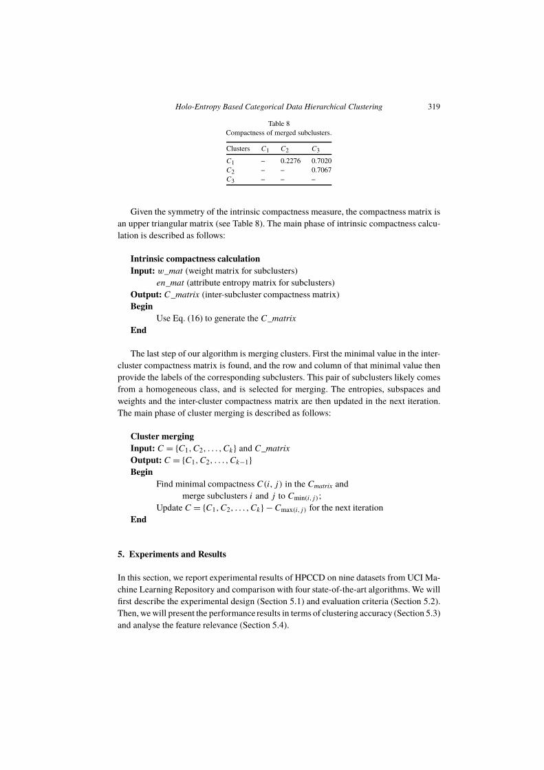
Holo-Entropy Based Categorical Data Hierarchical Clustering 319
Table 8
Compactness of merged subclusters.
Clusters C1 C2 C3
C1 – 0.2276 0.7020
C2 – – 0.7067
C3 – – –
Given the symmetry of the intrinsic compactness measure, the compactness matrix is
an upper triangular matrix (see Table 8). The main phase of intrinsic compactness calcu-
lation is described as follows:
Intrinsic compactness calculation
Input: w_mat (weight matrix for subclusters)
en_mat (attribute entropy matrix for subclusters)
Output: C_matrix (inter-subcluster compactness matrix)
Begin
Use Eq. (16) to generate the C_matrix
End
The last step of our algorithm is merging clusters. First the minimal value in the inter-
cluster compactness matrix is found, and the row and column of that minimal value then
provide the labels of the corresponding subclusters. This pair of subclusters likely comes
from a homogeneous class, and is selected for merging. The entropies, subspaces and
weights and the inter-cluster compactness matrix are then updated in the next iteration.
The main phase of cluster merging is described as follows:
Cluster merging
Input: C = {C1,C2, . . . ,Ck} and C_matrix
Output: C = {C1,C2, . . . ,Ck−1}
Begin
Find minimal compactness C(i, j) in the Cmatrix and
merge subclusters i and j to Cmin(i,j);
Update C = {C1,C2, . . . ,Ck} − Cmax(i,j) for the next iteration
End
5. Experiments and Results
In this section, we report experimental results of HPCCD on nine datasets from UCI Ma-
chine Learning Repository and comparison with four state-of-the-art algorithms. We will
first describe the experimental design (Section 5.1) and evaluation criteria (Section 5.2).
Then, we will present the performance results in terms of clustering accuracy (Section 5.3)
and analyse the feature relevance (Section 5.4).
320 H. Sun et al.
Table 9
UCI dataset description.
Dataset name Number of objects Number of attributes Number of classes
name objects attributes classes
Soybean 47 35 4
Votes 435 16 2
Mushroom 8124 22 2
Nursery 12960 8 4
Zoo 101 16 7
Chess 3196 36 2
Hayes-roth 132 4 3
Balance scale 625 4 3
Car evaluation 1728 6 4
5.1. Experimental Design
Besides the HPCCD algorithm, we tested four state-of-the-art algorithms, MGR (Qin et
al., 2014), K-modes (Aggarwal et al., 1999), COOLCAT (Barbar et al., 2002) and LIMBO
(Andritsos et al., 2004), for comparison with HPCCD. The choice of these algorithms
for comparison is based on the following considerations. MGR (Mean Gain Ratio) is a
divisive hierarchical clustering algorithm based on information theory, which performs
clustering by selecting a clustering attribute based on the mean gain ratio and detecting an
equivalence class on the clustering attribute using the entropy of clusters. The partition-
based K-modes algorithm is one of the first algorithms for clustering categorical data and is
widely considered to be the benchmark algorithm. COOLCAT is an incremental heuristic
algorithm based on information theory, which explores the relationships between dataset
and entropy, since clusters of similar POIs (Points Of Interest) yield lower entropy than
clusters of dissimilar ones. LIMBO is an Information Bottleneck (IB)-based hierarchical
clustering algorithm which quantifies the relevant information preserved when clustering.
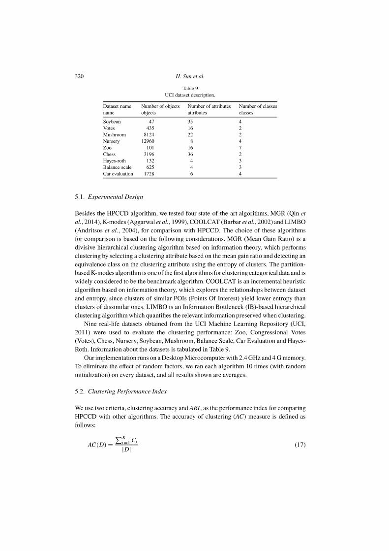
Nine real-life datasets obtained from the UCI Machine Learning Repository (UCI,
2011) were used to evaluate the clustering performance: Zoo, Congressional Votes
(Votes), Chess, Nursery, Soybean, Mushroom, Balance Scale, Car Evaluation and Hayes-
Roth. Information about the datasets is tabulated in Table 9.
Our implementation runs on a Desktop Microcomputerwith 2.4 GHz and 4 G memory.
To eliminate the effect of random factors, we ran each algorithm 10 times (with random
initialization) on every dataset, and all results shown are averages.
5.2. Clustering Performance Index
We use two criteria, clustering accuracy and ARI , as the performance index for comparing
HPCCD with other algorithms. The accuracy of clustering (AC) measure is defined as
follows:
AC(D) =
∑Ki=1
Ci
|D|(17)
Holo-Entropy Based Categorical Data Hierarchical Clustering 321
where |D| is the number of objects in the dataset, K is the number of classes in the test
dataset, and Ci is the maximum number of objects in cluster i belonging to the same
original class in the test dataset, i.e. the majority class.
For the sake of comparing clustering results against external criteria, we introduce
another clustering criterion, the Adjusted Rand Index (ARI) (Hubert and Arabie, 1985;
Yeung and Ruzzo, 2001). For better cluster validation, ARI is a measure of agreement
between two partitions, one being the clustering result and the other the original classes.
Given a dataset with n objects, suppose U = {u1, u2, . . . , us} and V = {v1, v2, . . . , vt }
represent the original classes and the clustering result, respectively. nij denotes the number
of objects that are in both class ui and cluster vi , while ui and vj are the numbers of objects
in class ui and cluster vi , respectively.
ARI =
∑
ij
( nij
2
)
−[∑
i
( ui
2
)∑
j
( vj
2
)]
/( n
2
)
1
2∗
[∑
i
( ui
2
)
+∑
j
( vj
2
)]
−[∑
i
( ui
2
)∑
j
( vj
2
)]
/( n
2
)
. (18)
The closer the clustering result is to the real classes, the larger the value of the cor-
responding ARI . Based on these two evaluation standards, we analyse the performance
of HPCCD and compare it with the other algorithms on nine real datasets from UCI. Fi-
nally, we also analyse the relationship between clusters and their relevant subspaces. By
introducing the concepts of principal features and core features, we demonstrate the ef-
fectiveness of the relevant subspaces.
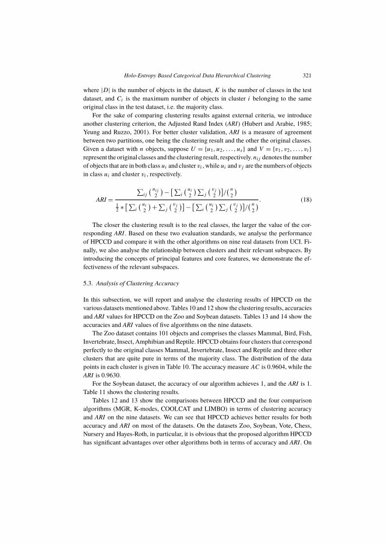
5.3. Analysis of Clustering Accuracy
In this subsection, we will report and analyse the clustering results of HPCCD on the
various datasets mentioned above. Tables 10 and 12 show the clustering results, accuracies
and ARI values for HPCCD on the Zoo and Soybean datasets. Tables 13 and 14 show the
accuracies and ARI values of five algorithms on the nine datasets.
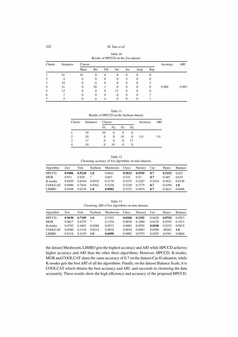
The Zoo dataset contains 101 objects and comprises the classes Mammal, Bird, Fish,
Invertebrate, Insect, Amphibian and Reptile. HPCCD obtains four clusters that correspond
perfectly to the original classes Mammal, Invertebrate, Insect and Reptile and three other
clusters that are quite pure in terms of the majority class. The distribution of the data
points in each cluster is given in Table 10. The accuracy measure AC is 0.9604, while the
ARI is 0.9630.
For the Soybean dataset, the accuracy of our algorithm achieves 1, and the ARI is 1.
Table 11 shows the clustering results.
Tables 12 and 13 show the comparisons between HPCCD and the four comparison
algorithms (MGR, K-modes, COOLCAT and LIMBO) in terms of clustering accuracy
and ARI on the nine datasets. We can see that HPCCD achieves better results for both
accuracy and ARI on most of the datasets. On the datasets Zoo, Soybean, Vote, Chess,
Nursery and Hayes-Roth, in particular, it is obvious that the proposed algorithm HPCCD
has significant advantages over other algorithms both in terms of accuracy and ARI . On
322 H. Sun et al.
Table 10
Results of HPCCD on the Zoo dataset.
Cluster Instances Classes Accuracy ARI
Mam Bir Fih Inv Ins Amp Rep
1 41 41 0 0 0 0 0 0
2 4 0 0 0 0 4 0 0
3 10 0 0 0 0 0 8 2
4 21 0 20 1 0 0 0 0 0.960 0.963
5 13 0 0 0 13 0 0 0
6 7 0 0 0 0 0 0 7
7 5 0 0 4 0 0 0 1
Table 11
Results of HPCCD on the Soybean dataset.
Cluster Instances Classes Accuracy ARI
D1 D2 D3 D4
1 10 10 0 0 0
2 10 0 0 10 0 1.0 1.0
3 17 0 0 0 17
4 10 0 10 0 0
Table 12
Clustering accuracy of five algorithms on nine datasets.
Algorithm Zoo Vote Soybean Mushroom Chess Nursery Car- Hayes- Balance-
HPCCD 0.9406 0.9218 1.0 0.8641 0.5823 0.5595 0.7 0.5152 0.652
MGR 0.931 0.828 * 0.667 0.534 0.53 0.7 0.485 0.635
K-modes 0.6930 0.8344 0.8510 0.5179 0.5475 0.4287 0.5410 0.4621 0.6336
COOLCAT 0.8900 0.7816 0.9362 0.5220 0.5228 0.3775 0.7 0.4394 1.0
LIMBO 0.9109 0.8230 1.0 0.8902 0.5222 0.4974 0.7 0.4621 0.6096
Table 13
Clustering ARI of five algorithms on nine datasets.
Algorithm Zoo Vote Soybean Mushroom Chess Nursery Car- Hayes- Balance-
HPCCD 0.9630 0.7109 1.0 0.5302 0.0260 0.2181 0.0428 0.0742 0.0923
MGR 0.9617 0.4279 * 0.1254 0.0036 0.1680 0.0129 0.0392 0.1011
K-modes 0.4782 0.4463 0.6586 0.0533 0.0082 0.0565 0.0540 0.0252 0.0915
COOLCAT 0.8586 0.3154 0.8214 0.0018 0.0018 0.0083 0.0500 .00261 1.0
LIMBO 0.8318 0.4159 1.0 0.6090 0.0082 0.0793 0.0285 0.0381 0.0684
the dataset Mushroom, LIMBO gets the highest accuracy and ARI while HPCCD achieves
higher accuracy and ARI than the other three algorithms. However, HPCCD, K-modes,
MGR and COOLCAT share the same accuracy of 0.7 on the dataset Car-Evaluation, while
K-modes gets the best ARI of all the algorithms. Finally, on the dataset Balance Scale, it is
COOLCAT which obtains the best accuracy and ARI , and succeeds in clustering the data
accurately. These results show the high efficiency and accuracy of the proposed HPCCD.
Holo-Entropy Based Categorical Data Hierarchical Clustering 323
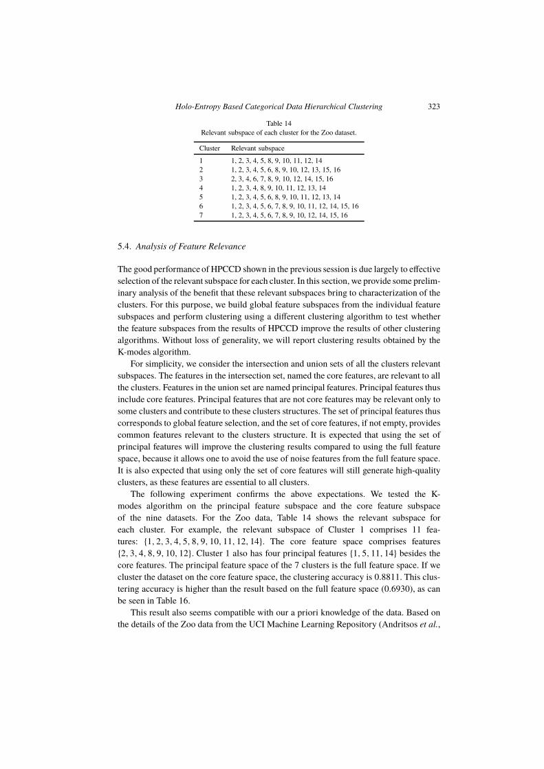
Table 14
Relevant subspace of each cluster for the Zoo dataset.
Cluster Relevant subspace
1 1, 2, 3, 4, 5, 8, 9, 10, 11, 12, 14
2 1, 2, 3, 4, 5, 6, 8, 9, 10, 12, 13, 15, 16
3 2, 3, 4, 6, 7, 8, 9, 10, 12, 14, 15, 16
4 1, 2, 3, 4, 8, 9, 10, 11, 12, 13, 14
5 1, 2, 3, 4, 5, 6, 8, 9, 10, 11, 12, 13, 14
6 1, 2, 3, 4, 5, 6, 7, 8, 9, 10, 11, 12, 14, 15, 16
7 1, 2, 3, 4, 5, 6, 7, 8, 9, 10, 12, 14, 15, 16
5.4. Analysis of Feature Relevance
The good performance of HPCCD shown in the previous session is due largely to effective
selection of the relevant subspace for each cluster. In this section, we provide some prelim-
inary analysis of the benefit that these relevant subspaces bring to characterization of the
clusters. For this purpose, we build global feature subspaces from the individual feature
subspaces and perform clustering using a different clustering algorithm to test whether
the feature subspaces from the results of HPCCD improve the results of other clustering
algorithms. Without loss of generality, we will report clustering results obtained by the
K-modes algorithm.
For simplicity, we consider the intersection and union sets of all the clusters relevant
subspaces. The features in the intersection set, named the core features, are relevant to all
the clusters. Features in the union set are named principal features. Principal features thus
include core features. Principal features that are not core features may be relevant only to
some clusters and contribute to these clusters structures. The set of principal features thus
corresponds to global feature selection, and the set of core features, if not empty, provides
common features relevant to the clusters structure. It is expected that using the set of
principal features will improve the clustering results compared to using the full feature
space, because it allows one to avoid the use of noise features from the full feature space.
It is also expected that using only the set of core features will still generate high-quality
clusters, as these features are essential to all clusters.
The following experiment confirms the above expectations. We tested the K-
modes algorithm on the principal feature subspace and the core feature subspace
of the nine datasets. For the Zoo data, Table 14 shows the relevant subspace for
each cluster. For example, the relevant subspace of Cluster 1 comprises 11 fea-
tures: {1,2,3,4,5,8,9,10,11,12,14}. The core feature space comprises features
{2,3,4,8,9,10,12}. Cluster 1 also has four principal features {1,5,11,14} besides the
core features. The principal feature space of the 7 clusters is the full feature space. If we
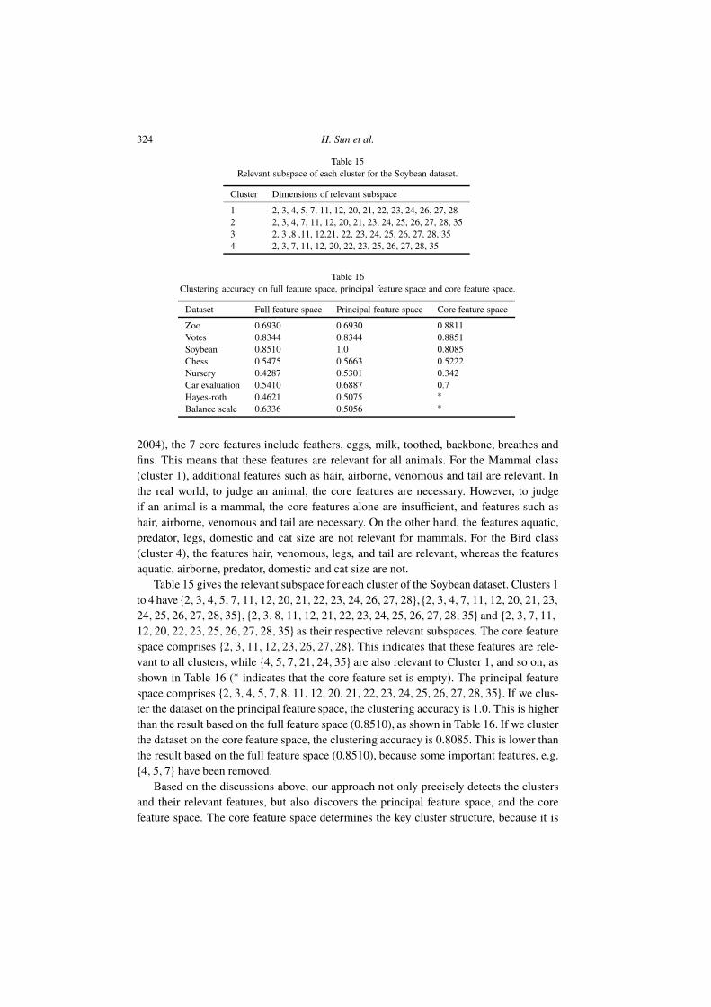
cluster the dataset on the core feature space, the clustering accuracy is 0.8811. This clus-
tering accuracy is higher than the result based on the full feature space (0.6930), as can
be seen in Table 16.
This result also seems compatible with our a priori knowledge of the data. Based on
the details of the Zoo data from the UCI Machine Learning Repository (Andritsos et al.,
324 H. Sun et al.
Table 15
Relevant subspace of each cluster for the Soybean dataset.
Cluster Dimensions of relevant subspace
1 2, 3, 4, 5, 7, 11, 12, 20, 21, 22, 23, 24, 26, 27, 28
2 2, 3, 4, 7, 11, 12, 20, 21, 23, 24, 25, 26, 27, 28, 35
3 2, 3 ,8 ,11, 12,21, 22, 23, 24, 25, 26, 27, 28, 35
4 2, 3, 7, 11, 12, 20, 22, 23, 25, 26, 27, 28, 35
Table 16
Clustering accuracy on full feature space, principal feature space and core feature space.
Dataset Full feature space Principal feature space Core feature space
Zoo 0.6930 0.6930 0.8811
Votes 0.8344 0.8344 0.8851
Soybean 0.8510 1.0 0.8085
Chess 0.5475 0.5663 0.5222
Nursery 0.4287 0.5301 0.342
Car evaluation 0.5410 0.6887 0.7
Hayes-roth 0.4621 0.5075 ∗
Balance scale 0.6336 0.5056 ∗
2004), the 7 core features include feathers, eggs, milk, toothed, backbone, breathes and
fins. This means that these features are relevant for all animals. For the Mammal class
(cluster 1), additional features such as hair, airborne, venomous and tail are relevant. In
the real world, to judge an animal, the core features are necessary. However, to judge
if an animal is a mammal, the core features alone are insufficient, and features such as
hair, airborne, venomous and tail are necessary. On the other hand, the features aquatic,
predator, legs, domestic and cat size are not relevant for mammals. For the Bird class
(cluster 4), the features hair, venomous, legs, and tail are relevant, whereas the features
aquatic, airborne, predator, domestic and cat size are not.
Table 15 gives the relevant subspace for each cluster of the Soybean dataset. Clusters 1
to 4 have {2,3,4,5,7,11,12,20,21,22,23,24,26,27,28}, {2,3,4,7,11,12,20,21,23,
24,25,26,27,28,35}, {2,3,8,11,12,21,22,23,24,25,26,27,28,35} and {2,3,7,11,
12,20,22,23,25,26,27,28,35} as their respective relevant subspaces. The core feature
space comprises {2,3,11,12,23,26,27,28}. This indicates that these features are rele-
vant to all clusters, while {4,5,7,21,24,35} are also relevant to Cluster 1, and so on, as
shown in Table 16 (∗ indicates that the core feature set is empty). The principal feature
space comprises {2,3,4,5,7,8,11,12,20,21,22,23,24,25,26,27,28,35}. If we clus-
ter the dataset on the principal feature space, the clustering accuracy is 1.0. This is higher
than the result based on the full feature space (0.8510), as shown in Table 16. If we cluster
the dataset on the core feature space, the clustering accuracy is 0.8085. This is lower than
the result based on the full feature space (0.8510), because some important features, e.g.
{4,5,7} have been removed.
Based on the discussions above, our approach not only precisely detects the clusters
and their relevant features, but also discovers the principal feature space, and the core
feature space. The core feature space determines the key cluster structure, because it is
Holo-Entropy Based Categorical Data Hierarchical Clustering 325
relevant to all clusters. This is very important in knowledge mining from high-dimensional
data.
6. Conclusions
Most hierarchical clustering algorithms tend to be based on similarity measures com-
puted on a common feature space, which is not effective for clustering high-dimensional
data. In this paper, we have proposed a new way of exploring information entropy, holo-
entropy, attribute selection and attribute weighting to extract the feature subspace and
merge clusters that have different feature subspaces. The new algorithm differs from ex-
isting mainstream hierarchical clustering algorithms in its use of a weighted holo-entropy
to replace the pairwise-similarity-based measures for merging two subclusters. The ad-
vantages of our algorithm are as follows: first, it takes interrelationships of the attributes
into account and avoids the conditional independence hypothesis, which is an implicit hy-
pothesis made by most existing hierarchical clustering algorithms. Secondly, it employs
the entropy and holo-entropy to detect the relevant subspace, and find the principal feature
space and the core feature space from the whole feature space of corresponding subclus-
ters. Thirdly, it uses intra-class compactness as a standard for merging subclusters rather
than the traditional similarity measurement. We performed experiments that demonstrate
the effectiveness of the new algorithm in terms of clustering accuracy and analysis of the
relevant subspaces obtained.
Acknowledgement. This project is supported by the National Natural Science Foundation
of China (61170130) and the State Key Laboratory of Rail Traffic Control and Safety
(Contract No. RCS2012K005), Beijing Jiaotong University).
References
Aggarwal, C.C., Yu, P.S. (2002). Redefining clustering for high dimensional applications. IEEE Transactions on
Knowledge and Data Engineering, 14(2), 210–225.
Aggarwal, C.C., Procopiuc, C., Wolf, J.L., Yu, P.S., Park, J.S. (1999). Fast algorithms for projected clustering.
In: Proceedings of the ACM SIGMOD 99, pp. 61–72.
Andritsos, P., Tsaparas, P., Miller, R.J., Sevcik, K.C. (2004). LIMBO: scalable clustering of categorical data.
Lecture Notes in Computer Science, 2992, 123–146.
Bai, L., Liang, J., Dang, C., Cao, F. (2011a). A novel attribute weighting algorithm for clustering high-
dimensional categorical data. Pattern Recognition, 44(12), 2843–2861.
Bai, L., Liang, J., Dang, C. (2011b). An initialization method to simultaneously find initial cluster and the number
of clusters for clustering categorical data. Knowledge and Information Systems, 24, 785–795.
Barbar, D., Li, Y., Couto, J. (2002). COOLCAT: an entropy-based algorithm for categorical clustering. In: Pro-
ceedings of the eleventh International Conference on Information and Knowledge Management. ACM, pp.
582–589.
Bouguessa, M., Wang, S. (2009). Mining projected clusters in high-dimensional spaces. IEEE Transactions on
Knowledge and Data Engineering, 21(4), 507–522.
Cao, F.Y., Liang, J.Y., Bai, L. (2009). A new initialization method for categorical data clustering. Expert Systems
with Applications, 33(7), 10223–10228.
326 H. Sun et al.
Choi, S., Ryu, B., Yoo, S., Choi, J. (2012). Combining relevancy and methodological quality into a single ranking
for evidence-based medicine. Information Sciences, 214, 76–90.
Cover, T., Hart, P. (1967). Nearest neighbor pattern classification. IEEE Transactions on Information Theory,
13, 21–27.
Cover, T., Thomas, J. (2012). Elements of Information Theory. John Wiley and Sons.
Derrac, J., Cornelis, C., Garca, S., Herrera, F. (2012). Enhancing evolutionary instance selection algorithms by
means of fuzzy rough set based feature selection. Information Sciences, 186, 73–92.
Do, H.J., Kim, J.Y. (2008). Categorical data clustering using the combinations of attribute values. In: Compu-
tational Science and Its Applications – ICCSA 2008, Series Lecture Notes in Computer Science, Vol. 5073.
pp. 220–231.
Domeniconi, C., Papadopoulos, D., Gunopulos, D., Ma, D. (2004), Subspace clustering of high dimensional
data. In; SDM 2004, pp. 73–93.
Filippone, M., Sanguinetti, G. (2010). Information theoretic novelty detection. Pattern Recognition, 43, 805–
814.
Fukunaga, K. (2013). Introduction to Statistical Pattern Recognition. Academic Press.
Gan, G., Wu, J. (2004). Subspace clustering for high dimensional categorical data. ACM SIGKDD Explorations
Newsletter, 6(2), 87–94.
Gan, G., Yang, Z., Wu, J. (2005). A genetic k-modes algorithm for clustering categorical data. Lecture Notes in
Computer Science, 3584, 195–202.
Gan, G., Wu, J., Yang, Z. (2009). A genetic fuzzy k-modes algorithm for clustering categorical data. Expert
Systems with Applications, 36, 1615–1620.
Ganti, V., Gehrke, J., Ramakrishnan, R. (1999). CACTUS: clustering categorical data using summaries. In:
Proceedings of the Fifth ACM SIGKDD International Conference on Knowledge Discovery and Datamining,
San Diego, CA, USA, pp. 73–83.
Greenacre. M, Blasius, J. (2006). Multiple Correspondence Analysis and Related Methods. CRC Press.
Guan, H., Zhou, J., Xiao, B., Guo, M., Yang, T. (2013). Fast dimension reduction for document classification
based on imprecise spectrum analysis. Information Sciences, 222, 147–162.
Guha, S., Rastogi, R., Shim, K. (1999). ROCK: a robust clustering algorithm for categorical attributes. In: Data
Engineering, 1999. Proceedings, 15th International Conference on IEEE, pp. 512–521.
He, Z., Xu, X., Deng, S. (2005). K-ANMI: a mutual information based clustering algorithm for categorical data.
Information Fusion, 9(2), 223–233.
He, Z., Xu, X., Deng, S. (2011). Attribute value weighting in k-modes clustering. Expert Systems with Applica-
tions, 38, 15365–15369.
Hruschka, E.R., Campello, R.J.G.B., de Castro, L.N. (2006). Evolving clusters in gene-expression data. Infor-
mation Sciences, 176(13), 1898–1927.
Huang, Z. (1998). Extensions to the k-means algorithm for clustering large data sets with categorical values.
Data Mining and Knowledge Discovery, 2(3), 283–304.
Huang, Z., Ng, M., Rong, H., Li, Z. (2005). Automated variable weighting in k-means type clustering. IEEE
Transactions on Pattern Analysis and Machine Intelligence, 27(5), 657–668.
Hubert, L., Arabie, P. (1985). Comparing partitions. Journal of Classification, 2(1), 193–218.
Jollois, F., Nadif, M. (2002). Clustering large categorical data. In: Proceedings of Pacific Asia Conference on
Knowledge Discovery in Databases (PAKDD02), pp. 257–263.
Kim, D., Lee, K., Lee, D. (2004). Fuzzy clustering of categorical data using fuzzy centroids. Pattern Recognition
Letters, 25(11), 1263–1271.
Li, Y., Zhu, S., Wang, X., Jajodia, S. (2006). Looking into the seeds of time: discovering temporal patterns in
large transaction sets. Information Sciences, 176(8), 1003–1031.
Li, H.X., Yang, J.-L., Zhang, G., Fan, B. (2013). Probabilistic support vector machines for classification of noise
affected data. Information Sciences, 221, 60–71.
Lingras, P., Hogo, M., Snorek, M., West, C. (2005). Temporal analysis of clusters of supermarket customers:
conventional versus interval set approach. Information Sciences, 172(1–2), 215–240.
Lu, Y., Wang, S., Li, S., Zhou, C. (2011). Particle swarm optimizer for variable weighting in clustering high
dimensional data. Machine Learning, 82(1), 43–70.
Nemalhabib, A., Shiri, N. (2006). Acm Symposium on Applied Computing, 2006, 637–638.
Parsons, L., Haque, E., Liu, H. (2004). Subspace clustering for high dimensional data: a review. ACM SIGKDD
Explorations Newsletter, 6(1), 90–105.
Holo-Entropy Based Categorical Data Hierarchical Clustering 327
Qin, H., Ma, X., Herawan, T., Zain, J.M. (2014). MGR: an information theory based hierarchical divisive clus-
tering algorithm for categorical data. Knowledge-Based Systems, 67, 401–411.
Sabit, H., Al-Anbuky, A., Gholamhosseini, H. (2011). Data stream mining for wireless sensor networks envi-
ronment: energy efficient fuzzy clustering algorithm. International Journal of Autonomous and Adaptive
Communications Systems, (4), 383–397.
Santos, F., Brezo, X., Ugarte-Pedrero, P., Bringas, G. (2013). Opcode sequences as representation of executables
for data-mining-based unknown malware detection. Information Sciences, 231, 64–82.
Schwenkera, F., Trentin, E. (2014). Pattern classification and clustering: a review of partially supervised learning
approaches. Pattern Recognition Letters, 37, 4–14.
Shannon, C.E. (1948). A mathematical theory of communication. The Bell System Technical Journal, XXVII(3),
379–423.
Shrivastava, N., Tyagi, V. (2014). Content based image retrieval based on relative locations of multiple regions
of interest using selective regions matching. Information Sciences, 259, 212–224.
Srinivasa, S. (2005). A review on multivariate mutual information. University of Notre Dame, Notre Dame,
Indiana, 2, 1–6.
Tan, S., Cheng, X., Ghanem, M., Wang, B., Xu, H. (2005). A novel refinement approach for text categorization.
In: Proceedings of the ACM 14th Conference on Information and Knowledge Management, pp. 469–476.
UCI Machine Learning Repository (2011). http://www.ics.uci.edu/mlearn/MLRepository.html.
Watanabe, S. (1960). Information theoretical analysis of multivariate correlation. IBM Journal of Research and
Development, 4, 66–82.
Wu, S., Wang, S. (2013). Information-theoretic outlier detection for large-scale categorical data. IEEE Transac-
tions on Knowledge and Data Engineering, 25(3), 589–601.
Xiong, T., Wang, S., Mayers, A., Monga, E. (2011). DHCC: divisive hierarchical clustering of categorical data.
Data Mining and Knowledge Discovery, 24(1), 103–135.
Yao, J., Dash, M., Tan, S.T., Liu, H. (2000). Entropy-based fuzzy clustering and fuzzy modeling. Fuzzy Sets and
Systems, 113(3), 381–388.
Yeung, K.Y., Ruzzo, W.L. (2001). Details of the adjusted Rand index and clustering algorithms, supplement to
the paper. An empirical study on principal component analysis for clustering gene expression data. Bioinfor-
matics, 17(9), 763–774.
Yip, K.Y.L., Cheng, D.W., Ng, M.K. (2004). HARP: a practical projected clustering algorithm. IEEE Transac-
tions on Knowledge and Data Engineering, 16(11), 1387–1397.
Yu, J., Lee, S.H., Jeon, M. (2012). An adaptive ACO-based fuzzy clustering algorithm for noisy image segmen-
tation. International Journal of Innovative Computing, Information and Control, 8(6), 3907–3918.
Zhang, C., Fang, Z. (2013). An improved K-means clustering algorithm. Journal of Information and Computa-
tional Science, 10(1), 193–199.
328 H. Sun et al.
H. Sun is a professor at the Department of Computer, Shantou University, China. His
main research interests are in data mining, machine learning, pattern recognition, etc.
R. Chen was awarded the candidate of master’s degree at computer science, Shantou
University, His main research interests include data mining, machine learning, pattern
recognition, etc.
Y. Qin is a professor in State Key Laboratory of Rail Traffic Control and Safety Beijing
Jiaotong University. The main research interest is intelligent transportation system, traffic
safety engineering, intelligent control theory.
S. Wang is a professor in Department of Computer Science University of Sherbrooke,
Canada. In research, he is interested in pattern recognition, data mining, bio-informatics,
neural networks, image processing, remote sensing, GIS. His current projects include
high-dimensional data clustering, categorical data clustering, data streams mining, pro-
tein and RNA sequences mining, graph matching and graph clustering, fuzzy clustering
and variable selection for data mining, location-based services, bankruptcy prediction,
business intelligence.