European

Historical

Economics

Society

EHES WORKING PAPERS IN ECONOMIC HISTORY | NO. 36

Household Debt and Economic Recovery

Evidence from the U.S. Great Depression

Katharina Gärtner

Free University Berlin, John-F.-Kennedy-Institute, Department of

Economics

MARCH 2013

EHES Working Paper | No. 36 | March 2013

Household Debt and Economic Recovery

Evidence from the U.S. Great Depression

Katharina Gärtner

Free University Berlin, John-F.-Kennedy-Institute, Department of

Economics *

Abstract The Great Recession has focused renewed attention on the role of household

leverage in the business cycle. Household debt overhang and the ensuing process of

deleveraging are often cited as factors holding back economic recovery. This paper

studies the relationship between household debt and economic performance during

the Great Depression in the U.S. on the state level. Using a newly compiled dataset,

I present evidence that debt overhang in the household sector acted as a severe drag

on economic recovery in the 1930s. States with higher initial debt-to-income ratios

recovered considerably slower. These findings point toward a close link between the

accumulation of debt and the severity and duration of recessions.

JEL codes: E2, E3, N22, R2

Keywords: Great Depression, household debt, mortgage finance, U.S.

Notice

The material presented in the EHES Working Paper Series is property of the author(s) and should be quoted as such.

The views expressed in this Paper are those of the author(s) and do not necessarily represent the views of the EHES or

its members

Acknowledgements: Versions of this paper were presented at Cambridge University (September 2012), London School

of Economics (December 2012), and Utrecht University (February 2013). The author is especially grateful

to Moritz Schularick, Irwin Collier, Martin Knoll, Ewout Frankema, and Lucais Sewell. I remain solely

responsible for the errors and interpretations.

* Katharina Gärtner, Free University Berlin, John-F.-Kennedy-Institute, Department of Economics, gaertner@gsnas.fu-

berlin.de

1 Introduction

Given the slow pace of economic recovery from the Great Recession in the U.S. andelsewhere, economists have begun examining the factors that keep economies depressedin the wake of financial crises.1 The speed of economic recovery continues to be a much-discussed topic in the media as well as in the economics profession. This debate hastypically focused on whether financial crises have been associated with deeper and moreprolonged spells of recession than other forms of crisis.

So far, two different interpretations of the historical evidence on recoveries from fi-nancial crises have been put forward. The first line of interpretation posits that financialcrises are associated with substantially weaker recoveries. Reinhart and Rogoff (2009a),for instance, argue in their widely cited work that declines in output, employment, andasset markets during recessions driven by financial crises are not only more pronouncedbut also significantly protracted (see also Reinhart and Rogoff (2009b)). Several authorssuch as Reinhart and Reinhart (2010), Cerra and Saxena (2008), and the InternationalMonetary Fund (2012) report similar findings, supporting the idea that financial criseshave a more adverse effect on economic performance during the period of recovery than“normal” recessions do.2 The second line of interpretation, however, contends that thereis little evidence for differences in output performance between different types of recessionduring the recovery period. On the contrary: it is even argued that the economy mightbounce back faster from deep recessions triggered by financial crises than recessions inwhich financial crisis has played no role (see Howard et al. (2011); Bordo and Haubrich

1In the 2012 U.S. presidential election the issue gained national importance when the economic recordof the outgoing administration became a matter of public and scholarly debate.

2Reinhart and Reinhart (2010) take a long-term perspective on financial crisis that incorporates therecovery period by examining the behavior of key macroeconomic indicators during the decade before andthe decade after the crisis. They find that financial crisis significantly adversely affect the performanceof these indicators, including slower income growth rates and elevated unemployment. Cerra and Saxena(2008), analyzing a sample of 160 countries, argue that financial crises are associated with large outputlosses that tend to be highly persistent. Based on this previous research, Reinhart and Rogoff (2012) arguethat the U.S. has performed better during the current recovery than during previous systemic financialcrises and has performed better than other countries that experienced similar systematic financial crisesin 2007–2008. Some critics, however, have pointed out that a sample such as used by Reinhart andRogoff (2009a), Reinhart and Reinhart (2010), and Cerra and Saxena (2008) comprising advanced anddeveloping economies might not offer meaningful evidence. Nevertheless, Schularick and Taylor (2012b),focusing on 14 advanced economies between the years 1870 and 2008, also stress that the recent recoveryhas been far better than could have been expected given the historical record on recoveries from financialcrises. From a sample of 21 advanced economies since 1960, the International Monetary Fund (2009)concluded that financial crisis-based recessions tend to be more severe and longer lasting than recessionsassociated with other shocks. The subsequent recovery is usually weaker, with tight credit conditionsand weak domestic demand being important features of these periods.

2

(2012)).3 Even though the general consensus is that recessions driven by financial crisisare more costly than other recessions (see for example Kaminsky and Reinhart (1999);Cerra and Saxena (2005a,b); Reinhart and Rogoff (2009b); Schularick and Taylor (2012a);Bordo and Haubrich (2010); Taylor (2012)), there remains some uncertainty about howrecoveries from financial crises differ qualitatively from recoveries associated with standardrecessions.4

While the explanatory power of the crisis type (i.e. financial or not) on the length,strength, and quality of recovery remains debated, recent research suggests that the devel-opment of certain macroeconomic variables during the pre-crisis period could be decisive.Schularick and Taylor (2012b) offer an insightful perspective using pre-crisis credit growthinstead of a binary approach to identify slumps set off by financial crises. The authorsconclude that “all recessions [and recoveries] are not created equal”: the more credit in-tense the expansion years preceding a crisis, the more severe the recession and the slowerthe recovery. This is particularly interesting because leverage has been identified as play-ing an important role in financial crises.5 In a similar vein, one strand of literature thatseeks to explain the current sluggish recovery stresses that high and persistent levels ofhousehold debt – known as a debt overhang – holds back economic recovery, becausehouseholds continue to deleverage in an attempt to repair their balance sheets (see Mianet al. (2011); Mian and Sufi (2012)).6

This paper aims to contribute to this debate. It offers a new perspective by analyzingthe link between high household indebtedness and economic performance during the re-covery from the Great Depression in the U.S. The Great Depression is an obvious placeto look. As in the run-up to the recent crisis, the years preceding the Great Depressionwere a time of marked credit expansion. Household indebtedness more than doubled inthe 1920s, from 15 percent of GDP in 1920 to 32 percent of GDP in 1929.7 After the

3Howard et al. (2011) examine 59 advanced and emerging economies since 1970. They define therecovery by indexing the level of GDP to 100 at the date of the recession trough. But they also note thatthe strength of recovery varies under certain circumstances. For instances, recessions featuring severehousing downturns are associated with slower recoveries, while deep recessions are followed by fasterrecoveries. Bordo and Haubrich (2012) analyze U.S. recessions since 1880. According to the authors,the weak current recovery is a major departure from historical precedent. Their approach, however, hasbeen criticized by Krugman (2012), who identifies several misattributions and argues that using growthfrom the recession trough as a measure of recovery success provides a blurred picture. This criticismalso applies to the approach used by Howard et al. (2011). Reinhart and Rogoff (2012) also observe thatBordo and Haubrich (2012) failed to distinguish between systemic financial crises and non-systemic ones.Schularick and Taylor (2012b) note that the implications of financial crises might be hard to identifygiven the small sample size when only focusing on U.S. experience.

4See also Brunnermeier and Sannikov (2012), who state that “[e]mpirically, the profession has notsettled the question of how fast recovery occurs after financial recessions.”

5See for example Tobin (1989), who called it the “Achilles heel of capitalism.” Sutherland et al. (2012)argue that high debt in general is associated with more pronounced vulnerabilities and thus can weakenmacroeconomic stability.

6See Konczal (2012) for an overview of studies discussing this balance sheet recession view.7Data drawn from Goldsmith (1955, Table D-1), Grebler et al. (1956, Table N4), James and Sylla

3

Great Crash in 1929, households tried to reduce their debt burdens (Temin, 1976, 171)as incomes fell.8 Aggregate demand collapsed, with consumer expenditures decreasing by18 percent between 1929 and 1933 (Temin, 1976, Table 1).9

In this paper, I use cross-sectional data for U.S. states to examine state-level variationin household indebtedness and the strength of recovery during the Great Depression. Thelevel of household debt varied substantially across states at the onset of the Depression.I look for evidence of a correlation between household debt and economic performanceduring the recovery period. The state-level focus not only allows a more detailed andnuanced study of the Great Depression in the U.S.; it is also helpful in circumventingproblems associated with unobserved heterogeneity in cross-country studies. In examiningthis relationship, I compiled a new dataset containing state-level data on credit, income,employment, and various other control variables for the period 1925–39.

I am not the first person to study state-level performance during the Depression withthe goal of understanding its specific drivers. Previous contributions have pointed outdifferences in economic structures and in initial prosperity as main factors that producespatial variation in economic performance (Wallis, 1989; Rosenbloom and Sundstrom,1997; Garrett and Wheelock, 2006). The role of New Deal spending and regional variationin banking crises has also been discussed in great detail (Fishback et al., 2003, 2005). It isthus important to control for a wide range of other factors. To the best of my knowledge,debt overhang in the household sector has not been examined systematically as a centralfactor behind the divergence in state-level economic performance in the 1930s. Therefore,this paper hopes not only to make a specific contribution to the aforementioned studieson the role of household debt in the business cycle but also to illuminate an importantaspect in the comparative development of U.S. states during the Great Depression.

The main findings of this paper are as follows. First, I demonstrate with a cross-sectional analysis that there was a close relationship between household indebtedness andeconomic performance during the recovery period. More indebted states showed worseeconomic performance than less indebted states. Second, I show that this indebted-ness/performance relationship was mostly driven by a slower pace of economic recovery,but not by a more severe recession. Thus, state-level data for the U.S. in the 1930s pro-vide strong evidence for the view that household indebtedness shapes the recovery path, a

(2006, Table 889), Schularick and Taylor (2012a).8Between 1929 and 1933, personal income per capita declined by about 35 percent in real terms (data

drawn from Schwartz and Graham (1955)).9Temin (1976) found that the collapse in aggregate consumption in 1930 was even more pronounced

than in 1921 and 1938 and argued that “the fall in consumption must be regarded as truly autonomous.”(Temin, 1976, 83). Examining the reasons of the collapse in consumption, Romer (1990) claimed that the1929 stock market crash created uncertainty about future income causing consumers to decrease spendingon durable goods. Olney (1999, 320) notes the significance of consumer debt, writing that “[t]he 1930drop in consumption resulted from the unique combination of historically high consumer indebtednessand punitive default consequences.”

4

view consistent with studies on debt overhang in the household sector during the currentrecession. Third, I present some suggestive evidence that deleveraging was an importantfactor as high debt-to-income states reduced their debts more strongly. My findings arerobust to the inclusion of controls for initial income levels, for sector-specific shocks, forbounce-back effects, for effects of fiscal and monetary policy, as well as for the degree ofbank distress. Overall, I find that household debt overhang is an important aspect inexplaining the severity and duration of the Great Depression in the U.S.

The remainder of this paper is structured as follows. Section 2 provides a theoreticaldiscussion, reviewing literature on the link between household debt, economic downturns,and subsequent recoveries. After discussing the dataset and the methodology, in section3 I analyze the relationship between household debt and economic performance duringthe 1930s. Moreover, I examine deleveraging as a possible transmission mechanism forthe adverse effect of high household indebtedness. The final section provides a summaryof my findings.

2 Household Debt and the Economy: Then and Now

In recent academic and political debates, the credit boom that preceded the Great Re-cession features prominently. This comes as no surprise, as it has been widely noted thatcountries experiencing particularly pronounced credit booms, such as the U.S. but alsothe United Kingdom and Spain, have faced more sluggish recoveries than countries likeGermany or Canada, which entered the Great Recession with low private credit levels.Using U.S. county level data, Mian, Rao, and Sufi (2011) and Mian and Sufi (2012) showhow the accumulation of household debt affected consumption and employment during therecession. They argue that the substantial accumulation of household debt between 2002and 2006 in combination with the collapse in home prices at the onset of the economiccrisis helps one to understand the onset, severity, and the length of the subsequent col-lapse in consumption (Mian et al., 2011). Faced with the strong decline in housing prices,highly leveraged counties experienced a severe shock to their balance sheets in 2007 and2008. Affected households started to reduce their debt burdens and rebuild their balancesheets. This, in turn, resulted in a significant drop in household consumption expendituresand pronounced weaknesses in aggregate demand. The researchers conclude that weakhousehold deleveraging and the resulting drop in aggregate demand were major causes ofthe high and persistent level of unemployment (Mian and Sufi, 2012).10 This relationship

10Both Mian et al. (2011) and Mian and Sufi (2012) employ U.S. county-level data for their studies.Using household survey data from the Panel Study of Income Dynamics, Dynan (2012) offers evidenceconsistent with this argument. Also Glick and Lansing (2009) make a similar point arguing that thedeleveraging by U.S. households would act as near-term drag on overall economic activity through aprolonged slowdown in consumer spending.

5

appears to apply not only to the United States but also to countries globally. Analyzinga sample of advanced economies over the past three decades, the International MonetaryFund (2012) finds that housing busts and recessions that were preceded by larger run-upsin household debt tended to be deeper and protracted.11

How can the close relationship between debt overhang in the household sector andeconomic performance be rationalized? This question is not entirely new. The role offinancial factors in the business cycle was the subject of research as far back as the 1930s.The boom leading up to the Great Depression was associated with a strong increase inhousehold indebtedness.12 While the literature emphasizes the rapid expansion of con-sumer credit during the années folles, caused by the consumer durable revolution (Vatter,1967) and the related proliferation of the installment plan (Olney, 1987; Hyman, 2011),mortgage debt as the largest component of total household liabilities increased at an evenslightly faster pace between 1920 and 1929.13 The rise in residential mortgage debt wasassociated with a nationwide real estate boom. Though prices probably peaked in 1925 –well in advance of the Great Depression – residential housing starts remained strong forthe rest of the decade, fueling a continuous rise in household mortgage debt.14

High levels of household debt accumulated during the 1920s were the principal ingre-dient to Irving Fisher’s concept of a self-enforcing debt deflationary spiral that reinforcesan initial economic shock (Fisher, 1933).15 According to Fisher, once household debt isperceived as excessive either by creditors or debtors, credit markets tighten and forcecreditors to consolidate by liquidating asset positions to reduce debt stocks. The subse-quent asset price slump increases the value of debt in real terms, enforcing another cycleof distress selling and debt-deflationary spiral. Accordingly, Fisher concludes that theGreat Depression was “an example of a debt-deflation depression of the most serious sort”(Fisher, 1933, 345).

Yet Fisher’s insights were largely forgotten in subsequent decades. Not only were thereno financial crises in advanced economies in the three decades after the Second World War.

11Already Glick and Lansing (2010) offer evidence that the link between rising leverage and rising houseprices since the late 1990s as documented by Mian and Sufi (2009) might be a global phenomenon. Thesame holds true for the link between household leverage before the crisis and the decline in consumptionduring the crisis.

12This unprecedented credit boom has been emphasized in several accounts of the 1920s (e.g. Allen(1931, 167 ff.)).

13Total consumer credit (i.e. long-term and short-term) increased from $6.07 bn in 1920 to $14.4 bnin 1929 for an average annual growth rate of 9 percent. During the same period, residential mortgagedebt rose from $7.2 bn to $18.9 bn, which amounts to an average annual growth rate of about 10 percent(data drawn from Goldsmith (1955, Table D-1), Grebler et al. (1956, Table N4), James and Sylla (2006,Table 889).

14For a discussion of the real estate boom and bust of the 1920s, see for example White (2009) andAllen (1931, 270 ff.).

15This was the first attempt to account systematically for the role of private debt in business cycletheory.

6

Fisher also neglected to discuss why changes in debt levels – which, by definition, go handin hand with equivalent changes in assets – have macroeconomic consequences. As everydebt is an asset for someone else, debt deflation episodes redistribute wealth, thoughthe aggregate asset position of the household sector remains more or less unchanged. Inshort, the unexpected price level shocks discussed by Fisher would only have redistributiveeffects within the household sector.

Tobin (1980, 10), focusing on the implications of distributional shocks between debtorsand creditors, asserts that “[a]ggregation would not matter if [...] the marginal propensityto spend from wealth were the same for creditors and debtors.” Tobin reasons that theborrower and lender status is not randomly distributed among households. Rather, thedebtor status indicates a comparably higher marginal propensity to spend. In this case,a redistribution of wealth from borrowers to lenders is not neutral in terms of demand.King (1994) further pursues Tobin’s argument, presenting suggestive evidence on the linkbetween the shortfall of consumption in the 1990s and the previous rise in the household-debt-to-income ratio by county and region for the United Kingdom. Another perspectivewas offered by Mishkin (1978), who argues that household balance sheet adjustments trig-gered by financial distress lower demand for tangible assets, which is to say, for consumerdurables and residential housing.16

The recent financial crises and the subsequent recession has precipitated renewed in-terest in these questions. Several recent contributions argue that a shock to householdbalance sheets results in a significant reduction in consumption (Hall, 2011; Eggerts-son and Krugman, 2011; Guerrieri and Lorenzoni, 2011; Philippon and Midrigan, 2011).Though this research focuses on the state of the household balance sheet, it differs fromMishkin (1978) in two regards: First, most authors define the shock to household balancesheets as a sudden credit tightening. Second, deleveraging is considered the main trans-mission mechanism linking high household debt to a decrease in consumption. In linewith Tobin (1980) and King (1994), these studies assume heterogeneous agents, i.e. thatsome households are borrowers and some are lenders.

Eggertsson and Krugman (2011) model a crisis that results from a deleveraging shocktriggered by sudden awareness that assets are overvalued and household collateral con-straints too lax, a so-called Minsky moment.17 The authors assume that households are

16In an earlier paper, Mishkin (1977) makes a similar point examining the 1973—75 recession. Inaddition to the ‘liquidity hypothesis,’ Mishkin (1978) tested Ando and Modigliani’s ‘life-cycle hypothe-sis.’ Based on this model, he reasons that a drop in a household net wealth has a significant impact onconsumption. Accordingly, the large drop in household net wealth between 1929 and 1930, further inten-sified by price deflation between 1930—32, might have contributed to the decline in aggregate demand.While this model does not distinguish between the effect of assets and the effect of liabilities on thehousehold balance sheet, debt deflation nevertheless partly explains why household net worth decreasedsubstantially during this period.

17This term goes back to Hyman Minsky and his financial instability hypothesis. Minsky argues thatthe economy is inherently unstable due to “capitalist finance” (Minsky, 1986, 219). He characterizes

7

heterogeneous: debtor households are impatient; creditor households are patient. As aconsequence of the sudden downward revision of acceptable debt levels, debtors need tocut back on current consumption to adjust to the borrowing constraint.18 Therefore, tosustain spending by the creditor so as to maintain a certain level of consumption, interestrates have to decrease. However, according to the authors, a nominal interest rate of zerocan still be too little to induce sufficient spending; hence, the economy may be stuck in aliquidity trap.19

Other models propose similar (if not identical) mechanisms. For instance, the modelof Guerrieri and Lorenzoni (2011) and the model of Eggertsson and Krugman (2011) bothassume that borrowers deleverage by reducing consumption, but the former also assumesthat lenders increase precautionary savings as well. Through the sudden reduction inthe demand for, and increase in, the supply of savings, interest rates fall and outputdeclines, with both effects being strongest in the short run.20 In related work, Philipponand Midrigan (2011) focus on housing as both a consumption good and as a meansof providing liquidity via home equity borrowing. When a shock limits the ability ofhouseholds to extract equity from their houses, leveraged households are forced to reducetheir consumption. Applying their model to the Great Recession, they conclude thata reduction in credit at the household level accounts for the decrease in output andemployment to a non-negligible extent.

While these theoretical and empirical contributions assume different transmissionmechanisms, they all agree that the buildup of debt in the household sector coupled witha shock to household balance sheets can contribute significantly to deep and prolongedeconomic downturns. The history of the Great Depression provides a fascinating testingground for these hypotheses. Before turning to the empirical evidence on the relationshipbetween household debt and state-level economic performance during the 1930s, however,

the business cycle upswing as a period of transitory tranquility that expands as economic agents becomeincreasingly optimistic, increasing the willingness to borrow and to engage in speculative and debt financepractices. As balance sheets deteriorate, financial fragility arises. The boom comes to an end when short-and long-term interest rates rise, creating the so-called the Minsky moment. Whether this later leadsto a deep recession, a financial crisis, or debt deflation depends mainly on structural characteristics andspecific policies, such as overall economic liquidity, government size, and lender-of-last-resort actions bythe central bank. The tendencies that precipitate a boom are also determined by institutional structuresand policy systems (Minsky, 1986, 197ff.). Though Minsky focuses on corporate debt, his hypothesis, orparts of it, have been applied to cases of household indebtedness by Eggertsson and Krugman (2011) andPalley (1994), among others.

18Way back in 1896 Bagehot noted that “[c]redit – the disposition of one man to trust another – issingularly varying. In England, after a great calamity, everybody is suspicious of everybody; as soon asthat calamity is forgotten, everybody again confides in everybody.”

19Hall (2011) makes a similar point, arguing that in an economy with a disabled monetary policy thedecline in aggregate demand driven by deleveraging is a major factor in understanding the nature of thecontraction.

20Contrary to the findings of Eggertsson and Krugman (2011), borrowing and lending are driven byidiosyncratic income shocks rather than by preferences, though Eggertsson and Krugman (2011) alsoincorporate a nominal debt deflation mechanism.

8

I present in the next section the dataset and discuss the methodology.

3 Estimating the Effects of Household Debt on Eco-

nomic Recovery in the 1930s

The trajectory of the Great Depression in the U.S. is well known. After the stock marketcrash in October 1929, the U.S. economy entered a sharp recession. In the second half of1932, industrial production increased slightly but a wave of banking failures in early 1933pushed the U.S. back into depression. It was only after the banking holiday in the springof 1933 that the recovery began in earnest. Until 1937, real GNP grew at an averageannual rate of over 8 percent. In the period 1937–38, the recession within the depressioninitiated new economic troubles. Despite the high growth rates throughout the recovery,the fall in output was so severe that the U.S. only returned to its pre-Depression growthpath around 1942 (see, e.g. Romer (1990, 1992)). The strength of the recovery differedsubstantially across U.S. states, however.

In this section, I study the role of household debt in the 1930s. The key question tobe addressed is whether there is systematic evidence that higher levels of indebtednesswere associated with slower recovery. The analysis will focus on state-level economic per-formance in the recovery period, i.e. from 1933 to 1939. Economic performance is definedusing four different indicators: personal income, wages, employment, and consumption.I also study other sub-periods and perform various robustness tests. The sub-periodsthat I examine are the Great Depression as a whole (1929–39), the contraction period(1929–32), as well as two periods excluding the recession within the Depression (1929–37and 1933–37). This differentiated approach reveals that the strong relationship betweenhousehold debt and economic performance is mostly due to a slower pace of economicrecovery and not to a more severe slump in the initial years of the Depression recession.

3.1 Data and Methodology

To study the effect of household debt on economic performance during the Great Depres-sion, I compiled a new dataset. The dataset covers 48 U.S. states and the District ofColumbia from the years 1929 to 1939 at annual frequency.21 For each state, it assemblesdata on household debt, on income and wages per capita, on employment for the period,on New Deal spending, on sectoral output composition, on discount rates set by the re-spective regional Federal Reserve Banks, on bank failures, and on retail sales. In doingso, I draw on a variety of data sources and the work of other scholars such as Fishback

21Alaska and Hawaii did not become U.S. states until 1959.

9

et al. (2005) and Wallis (1989). Below I briefly describe the key variables and introducethe empirical model to be estimated.22

For the period of the Great Depression and the subsequent recovery, most standardindicators for economic performance and business cycle activity (e.g. GDP, consumption)are unavailable due to lack of reliable and consistent state-level data. To circumventthis shortcoming, I use state-level per capita income (INCs) and per capita salaries andwages (WAGEs) as dependent variables. While at the national level, per capita income23

serves as a good proxy for GDP per capita (correlation coefficient of 0.98 for the period1929—39), per capita salaries and wages (the largest share of total household income)are a more sensitive income measure of economic fluctuations.24 I draw data on totalhousehold income and salaries and wages from Schwartz and Graham (1956). To studythe effects of household debt on employment, I also use the employment index providedby Wallis (1989) (EMPs) as a third dependent variable. The index is calculated fromestablishment surveys on firms undertaken by the Bureau of Labor Statistics (BLS).25

According to Fishback et al. (2005), retail sales serve as a strong proxy for consumption,both for durable and non-durable goods. As a fourth dependent variable, therefore, I usedata on retail sales supplied by Fishback et al. (2005) to examine effects on consumption(SALESs).

In the empirical literature examining the effects of indebtedness on economic perfor-mance, the household debt-to-income ratio is commonly used as key explanatory variable(see, e.g., Olney (1999), Glick and Lansing (2010), Mian et al. (2011), Philippon andMidrigan (2011), International Monetary Fund (2012), Mian and Sufi (2012)). I use theaverage state-level ratio of household debt-to-income in 1929 (DEBTs,1929) to proxy forhousehold leverage.26

As data on total household debt is unavailable at the state level, average annual debt-to-income ratios are calculated using annual state-level mortgage debt data drawn fromthe All Bank Statistics (ABS) (Board of Governors of the Federal Reserve System, 1959).In assessing the adequacy of the approximation, I calculated the share of total residentialmortgage debt, the share of national-level mortgage debt, and the share of household debt.

22For a complete description of data, see Appendix B.23Personal income comprises wages and salaries, supplementary types of labor income such as employer

contributions to private pension, net proprietor’s income for unincorporated businesses, property income,and transfer payments.

24Wage and salary disbursements accounted for on average 58.5–65.2 percent of personal income in the1930s (see Creamer and Merwin (July 1942, 23)).

25The index base year is 1929 (100) (Wallis, 1989).26I use the word leverage in a broader sense to stand for household indebtedness relative to income.

Typically, the concept of leverage relates to the ratio of household debt to household assets. In the eventof an adverse economic shock, households with an unexpected debt overhang are forced to readjust totheir targeted net asset position through deleveraging. By leverage I generally mean the debt-to-incomeratio or income leverage. “Debt overhang” also refers to the debt-to-income ratio of households.

10

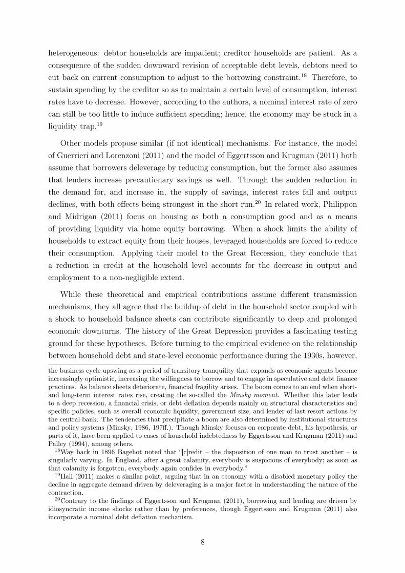
As shown in Figure 1, mortgage debt is by far the largest share of household debt duringthe period 1925–39, amounting to on average 60 percent of total household debt. At thenational level, mortgage debt reproduces the trends and fluctuations in total householddebt fairly well, with a variable correlation of 0.8.

0.2

.4.6

.81

1925 1926 1927 1928 1929 1930 1931 1932 1933 1934 1935 1936 1937 1938 1939

Residential Mortgage Debt (in % of total) Consumer Debt (in % of total)

Figure 1: Shares of Nonfarm Private Debt,1925–39 Source: James and Sylla (2006,Tables 889); Goldsmith (1955, Table D-1);Grebler et al. (1956, Table N4).

-.1-.0

50

.05

.1.1

51925 1926 1927 1928 1929 1930 1931 1932 1933 1934 1935 1936 1937 1938 1939

Annual Percentage Change - Real Estate Lending All Bank Statistics Annual Percentage Change - Total Residential Mortgage Debt Outstandin

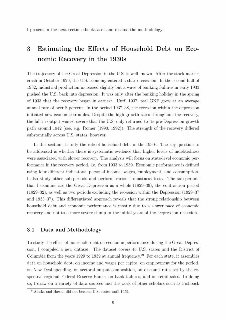
Figure 2: Total Annual PercentageChange for U.S. Mortgage Debt Out-standing and All Bank Statistics Real Es-tate Lending, 1925–39 Source: All BankStatistics; Grebler et al. (1956, Table N4)

Yet data from the ABS suffer from two constraints: First, they underestimate totalmortgage debt because they do not record household lending by all financial intermedi-aries. The ABS cover mortgages issued by national banks, chartered state banks, loanand trust companies, stock savings banks, unincorporated private banks, and mutual sav-ings banks. This neglects major lenders for mortgage credit such as building and loanassociations and life insurance companies. Second, the data series also comprises loanson farmland and other properties, as well as loans on bonds and mortgages.27

Nevertheless, real estate lending as reported by in the ABS appears to be a goodindicator for total residential mortgage lending. Figure 2 compares annual percentagechanges in the ABS on national level with annual percentage changes in total residentialmortgage debt outstanding as reported by Grebler et al. (1956). As is quite evident,the two data series follow the same trend for the national level. Both series are stronglycorrelated (approx. 0.8) for the period 1925–39.

Figure 2 also confirms the strong increase in mortgage indebtedness during the sec-27For instance, the share of farm mortgages was between 20 and 30 percent of total mortgages during

the period 1925-–39.

11

ond half of the 1920s.28 Data drawn from the ABS suggest a strong positive relationshipbetween the mortgage debt-to-income level in 1929 and the percentage change in mort-gage debt per capita from 1925 to 1928.29 Unsurprisingly, this indicates that householdshad higher debt-to-income ratios when the boom years came to an end in states with aparticularly pronounced credit growth in the 1920s.30

The key explanatory variable in the following analysis is the initial average state-levelindebtedness of households, DEBTs,1929, defined as the mortgage debt-to-income ratio asof 1929 for each state. As a robustness check, I also use the mortgage debt-to-income ratioas of 1932 (DEBTs,1932) for each state. Results for these two key variables are reportedseparately in section 3.2, but the results are very similar.

Debt levels are unlikely to be the only drivers of economic performance, however.Hence, it is crucial to account for other factors that may produce spatial inequality ineconomic performance and propose additional control variables. In selecting variables Ifollow previous literature (see for example Calomiris and Mason (2003), Romer (1993, 32ff.), Fishback et al. (2005, 38), Garrett and Wheelock (2006)). The control variables fallinto the following broad categories: income level, fiscal policy, and the effects of the NewDeal; sector specific factors; potential regional differences in monetary policy; and bankfailures.

Let me now discuss the other factors that may have induced spatial inequality andthe control variables needed to compensate for them. I have five salient points. First,the depression could have had different effects on states depending on their productivitylevels, which is why I include – state-level income per capita in 1933 relative to nation-wideincome per capita in 1933 – as a measure of aggregate productivity.

Second, since bank failure rates vary widely across states, BANKFAILs controls forthe degree of bank distress at the state level between 1929 and 1933 and is defined asthe annual average rate of bank suspensions in the period 1929—33.31 Although the ex-act transmission mechanism through which bank failures magnify the extent of economic

28This applies to all loan categories reported in the ABS: real estate loans, loans secured by collateralother than real estate, and all other loans (see Table 9). The increase in real estate loans and loans oncollateral (including loans backed by securities) stands out in particular and provides a suggestive linkbetween the real estate boom and the stock market boom and the growth of credit.

29The correlation coefficient is 0.43. The relationship remains strong (corr. 0.48) even when omittinginfluential observations (VT, MA, NH, CT, NY). This also applies when using the change in total loansp.c. as reported in the ABS 1925—28 (corr. 0.40). But because state-level income data is unavailableprior to 1929, it is impossible to determine the extent to which the increase in household debt correspondsto a comparable development in income.

30In Oklahoma, households were the lowest income levered (with a mortgage debt-to-income ratio of0.13). Households were the highest income levered in Vermont (with a mortgage debt-to-income ratio of0.43).

31While most northeastern states had low failure rates, several mid-western and southern states facedsubstantial bank distress, with failure rates exceeding ten percent in the period 1929—33.

12

decline is disputed,32 bank failures have been identified as a significant factor in explain-ing economic performance during the period of the Great Depression (see, for example,Friedman and Schwartz (1963), Bernanke (1983), Calomiris and Mason (2003), Romer(1993, 32 ff.)). Bank failures might matter particularly as an indicator of credit supply(see Calomiris and Mason (2003)).

Third, during the 1930s, particularly as part of the New Deal, the federal governmentembarked on expansionary fiscal policy and issued substantive volumes of loans and grantsthroughout the United States to revive economic activity. As a result, federal civilianspending as a share of GNP increased from about one to eight percent during this decade(Rockoff, 1998, 130). Because New Deal spending per capita differed markedly acrossstates (see for example Fishback et al. (2005, 38)), I control for cross-sectional leveleffects with the variableNEWDEALs, which measures cumulative per capita governmentspending and lending from 1933 to 1939 for each state.

Fourth, sector-specific shocks might create spatial differences in economic performancedepending on the sectoral composition of output in a respective state. Sectors particularlyaffected by the economic downturn after 1929 were agriculture, mining, construction,and durable manufacturing. By contrast, the services and transportation sector wereaffected to a lesser extent (Garrett and Wheelock, 2006, 464). Accordingly, states with aninitially unfavorable sectoral specialization can be expected to experience larger declinesin per capita income than states less dependent on these sectors. I use AGRICs,1929 andMANs,1929 to proxy for sector specific factors. These variables measure salaries and wagesreceived from agriculture and manufacturing as a share of total personal income at thestate level in 1929.33

Fifth, and finally, I aggregated states into regions based on the Federal Reserve Dis-tricts as a control variable. It measures the extent and timing of the monetary policyresponse by the respective regional Federal Reserve Bank (MONPOLs) to account forpossible differences in monetary policy. The variable is calculated using data on discountrates set by the respective regional Federal Reserve Banks in the contraction period, i.e.1929–32. Timing and scale of interest rate cuts are used as weights. Earlier and strongerinterest rate cuts are attributed a higher weight than smaller and posterior reductions indiscount rates. The results suggest that differences in monetary policy generally did notproduce spatial variation in economic outcomes.

32Friedman and Schwartz (1963), for example, point out the negative impact of banking panics onmoney supply, which led to a decline in spending, employment, and output. Bernanke (1983), by contrast,argues that the principal conduit for the transmission of shocks is that of disrupted credit flows throughthe increased cost of financial intermediation.

33In 1929, about 25 percent of national income came from salaries and wages in the manufacturingsector and about 10 percent from salaries and wages in the agricultural sector (data drawn from Carter(2006)).

13

Summary statistics for the main variables are presented in Table 1.

Table 1: Summary StatisticsMean Min Max Std. Dev. N

DEBTs,1929 0.0986 0.0130 0.4259 0.0953 49∆INCs (1929–39) 0.0107 -0.2012 0.2104 0.0836 49∆WAGEs (1929–39) 0.0626 -0.3238 0.3040 0.0956 49∆EMPs (1931–39) 0.1624 0.0812 0.0178 0.3907 48∆SALESs (1929–39) 0.0100 -0.3027 0.2302 0.1268 48DELEVs 0.0793 -0.5230 1.1480 0.3481 48NEWDEALs (in 1967$) 238.27 107.46 746.78 111.21 49BANKFAILs 0.1340 0.0081 0.3944 0.0829 49

I use a cross-sectional OLS model. The estimation equation for the baseline specifica-tion covering the period 1933–39 is:

∆Ys = α + β1DEBTs,1929 + β2INCs,1933 + β3AGRICs,1929 + β4MANs,1929

+ β5NEWDEALs + β6MONPOLs + εs (1)

with s indexing states. The error term is assumed to be well behaved. ∆Ys varies inthe regressions. I use four different dependent variables: income per capita, salaries andwages per capita, employment, and retail sales. ∆Ys is

∆Ys = lnYs,1937 − lnYs,1933 (2)

In other words, it expresses the observed percentage change of the respective dependentvariable during the recovery period. This period also covers the recession within thedepression and might thus confuse different effects. For this reason, the specification isestimated to exclude the years 1938 and 1939 as a second measure of the recovery period.

3.2 Household Debt and Recovery, 1933–39

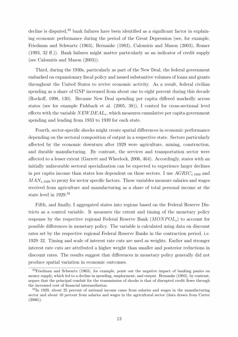
What were the implications of high ex-ante levels of household income leverage for eco-nomic performance during the recovery period? The initial visual inspection of the datasuggested a notable relationship between the level of household indebtedness as of 1929and the growth rate in personal income between 1933 and 1939. Figure 3 shows thecorrelation plot for these two variables. The plot indicates that high-debt states showedworse economic performance than lower indebted states.34

While the relationship in Figure 3 is indicative, one also needs to control for other34This negative relationship remains robust even when omitting the influential states VT, MA, NH,

NY, CT, and PA.

14

AK

AL

AZ

CACOCT

DC

DE

FL

GA

IA

ID

IL

IN

KSKY

LA

MA

MD

ME

MI

MN

MO

MS

MT

NC

ND

NE

NH

NJ

NMNV

NY

OHOK

OR

PA

RI

SC

TN

TX

UTVA

VT

WA

WIWV

WY

.2.3

.4.5

.6.7

0 .1 .2 .3 .4Mortgage Debt to Income 1929

%Change in Personal Income 1933-1939 Fitted values

Figure 3: Debt to Income 1929 and Percentage Change in Personal Income 1933–1939.Source: Board of Governors of the Federal Reserve System (1959); Schwartz and Graham(1956).

variables, as I stress above. I thus now turn to formal regression analysis using thebaseline specification outlined in the previous subsection.

Table 2 shows the regression of ex-ante household indebtedness on the percentagechange in four indicators for economic performance from 1933 to 1939: income percapita, wages per capita, employment, and retail sales. The model is estimated withheteroskedasticity-robust standard errors.35 These benchmark results show an interestingpicture: regression coefficients on DEBTs,1929 are negative and highly significant on thefive percent level for all dependent variable specifications. Everything else being equal, thecoefficients point toward a decrease in the growth rate of employment, per capita income,and per capita salaries and wages during the recovery between 2.7 and 4.2 percentagepoints for a debt-to-income ratio ten percentage points above the sample mean. At thevery least, these preliminary results suggest that in states where households initially facedrelatively high debt balances, economic performance between 1933 and 1939 was markedlyweaker.

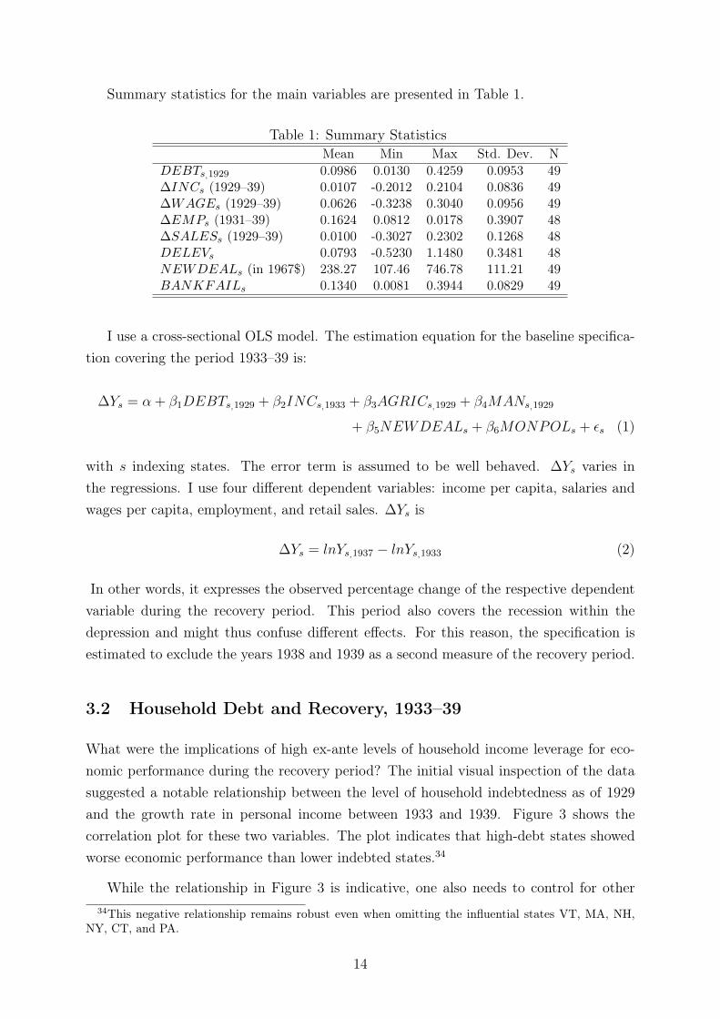
Figure 4 explores this relationship between the level of household indebtedness and thestrength of economic recovery in simple graphical form. The graphs present an index with1933=100 for all four dependent variables distinguishing between the 13 high-debt statesand the 12 low-debt states, i.e. the states in the top and bottom quartile for the 1929debt-to-income ratio. It shows a clear divergence of recovery paths in these two groups

35Standard errors and levels of significance are not distorted by heteroskedasticity because standardtest procedures (like the Breusch-Pagan test) do not detect it. This assumption is also supported by thefact that regressions with and without heteroskedasticity-robust standard errors and levels of significancedo not differ significantly. All regression results in this paper are reported with heteroskedasticity-robuststandard errors and levels of significance. For income p.c., SD has been omitted as an outlier. Wallis(1989) does not provide an employment index for DC in any given year.

15

for all economic performance indicators. Overall, low-debt states appear to recover fasterand stronger during the period 1933–39.36

100

110

120

130

140

1933 1934 1935 1936 1937 1938 1939Year

High Debt States Low Debt States

Employment Index (1933=100)

100

120

140

160

1933 1934 1935 1936 1937 1938 1939Year

High Debt States Low Debt States

Income p.c. Index (1933=100)

100

1101

2013

0140

1933 1934 1935 1936 1937 1938 1939Year

High Debt States Low Debt States

Wages p.c. Index (1933=100)

100

120

140

160

1933 1934 1935 1936 1937 1938 1939Year

High Debt States Low Debt States

Retail Sales Index (1933=100)

Figure 4: Recovery in Employment, Income p.c., Wages p.c., and Retail Sales for High-Debt and Low-Debt States Source: Board of Governors of the Federal Reserve System(1959); Schwartz and Graham (1956); Fishback et al. (2005); Wallis (1989).

According to the regression results in Table 2, the level of per capita income in 1933correlates negatively to economic performance in the recovery period. This means that theinitially less prosperous states experienced a stronger recovery. The immediate question,however, is how these less prosperous states performed during the contraction period. Ifthey performed worse than more prosperous states – due to a sectoral composition thatmade the state economy more vulnerable to shocks, say – the negative effect of incomeper capita as of 1933 may be due to catch-up or bounce-back effects. In the “pluckingmodel” of business fluctuations, Friedman (1993) argues that the size of the contractionaffects the subsequent expansion and thus hypothesizes a bounce-back effect. For thisreason, I include an additional control for a bounce-back effect (BOUNCEBACKs) thatis calculated as the percentage change (change in natural logs) of the respective dependentvariable in the period 1929–32.37

Table 3 repeats the benchmark regression of Table 2 when controlling for a bounce-backeffect. Regression coefficients on DEBTs,1929 in columns (1) to (4) remain negative andhighly significant on the five percent level for all dependent variable specifications.38 All

36Accordingly, the 12 low-debt states are CO, ID, KS, MT, NE, NM, OK, OR, PA, SD, TX, and WY.The 13 high-debt states are CA, CT, IA, MA, ME, MI, NH, NJ, NY, OH, RI, UT, and VT.

37The respective BOUNCEBACKs variables are defined as ∆INCs,1929−32 = lnINCs,1932 −lnINCs,1929, ∆SALs,1929−32 = lnSALs,1932 − lnSALs,1929 and ∆EMPs,1929−30 = lnEMPs,1930 −lnEMPs,1929. Since no data is available for retail sales in 1932, ∆INCs,1929−32 = lnINCs,1932 −lnINCs,1929 will be used as a proxy for the bounce-back effect in retail sales. The growth rates inretail sales and personal income strongly correlate for the period 1929—39 (corr. 0.64).

38To test for the robustness of this relationship, I have analyzed other periods of recovery as well:1933–36, 1934–36, and 1934–37. The negative correlation between initial household debt and economicperformance remains robust and significant.

16

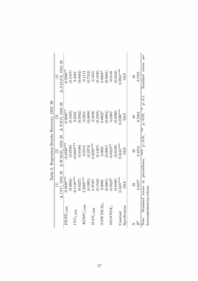
Table2:

RegressionResults

Recovery,

1933

–39

(1)

(2)

(3)

(4)

∆INCs19

33–3

9∆

WAGE

s19

33–3

9∆

EM

Ps19

33–3

9∆

SALESs19

33–3

9DEBTs ,1929

-0.282

0***

-0.232

0***

-0.388

0**

-0.320

6**

(0.086

2)(0.078

6)(0.150

5)(0.135

7)INCs ,1933

-0.112

0***

-0.088

3***

0.02

220.43

84(0.022

7)(0.016

6)(0.056

2)(0.048

2)AGRICs ,1929

2.32

08**

*-0.051

4-0.295

1-0.111

4(0.199

5)(0.237

4)(0.680

8)(0.755

2)M

AN

s ,1929

0.2726

*0.32

30**

*-0.283

0-0.105

5(0.155

6)(0.126

7)(0.250

5)(0.183

0)NEW

DEALs

0.00

000.00

010.00

02*

0.00

02*

(0.000

1)(0.000

1)(0.000

1)(0.000

1)M

ONPOLs

-0.032

3*-0.032

3**

-0.026

7-0.014

8(0.016

8)(0.013

9)(0.029

0)(0.024

4)Con

stan

t0.3427

***

0.34

45**

*0.25

96***

0.39

41***

Specification

OLS

OLS

OLS

OLS

N48

4948

48R

20.64

770.43

140.23

840.17

65Note:

Stan

dard

errors

inpa

renthe

ses;

***

p<0.01

,**

p>0.05,

*p<

0.1.

Stan

dard

errors

are

heteroskedasticity-rob

ust.

17

things being equal, the coefficients suggest a decrease in the growth rate of employment,retail sales, per capita income, and per capita salaries and wages during the recoverybetween 2.2 and 3.2 percentage points for a debt-to-income ratio ten percentage pointsabove the sample mean for the period 1933–39. Moreover, the explanatory power ofthe specification is substantive, explaining up to about 69 percent of the regressand’svariation. The null hypothesis of the F-test can clearly be rejected for all specificationsexcept for regression (4).39 Even though the model has weak explanatory power forSALESs, the results suggest a statistically significant relationship between high initialhousehold indebtedness and the decline in consumption during the period 1933–39. Yetbecause the availability of retail sales data for the period 1929–39 is insufficient for makingreliable conclusions, these findings provide suggestive evidence at best.40 Nevertheless,the results provide some indication that highly indebted households cut back consumptionmore strongly than households with lower levels of indebtedness.

The period 1933–39 includes the effects of the 1937 recession and hence might beconfusing different effects. To extend the analysis, I use regressions (5) to (7) to examinethe time period 1933–37 but excluding the effects of the 1937 recession. Since no dataon retail sales is available for 1937, SALESs is omitted as a dependent variable.41 Ascan be seen, the results hold up: regression coefficients on DEBTs,1929 are negative andstatistically significant on the one percent level for (5) and (6).42 Once again, the modelhas high explanatory power. These regressions confirm the findings presented in Table 2suggesting that in states where households initially faced comparably high debt balances,economic performance between 1933 and 1937 as well as between 1933 and 1939 wasmarkedly weaker. The results remain significant when including weights for state size, i.e.when measured by state population in 1930 (see Appendix, Table 14).

As for the other control variables in Table 3, the results indicate that there is indeed astrong bounce-back effect: states that had suffered more pronounced losses in income andemployment during the slump experienced a stronger and more rapid recovery.43 This isin line with previous findings. For instance, Rosenbloom and Sundstrom (1997) attribute

39The F-value is 27.53 in column (1), 8.34 in column (2), 5.68 in column (3), 2.48 in column (4), 22.68 incolumn (5), 4.29 in column (6) and 6.39 in column (7) with respective p-values of about 0.00. (Except forcolumn (4), where the p-value is 0.03.) The F-test is not distorted by multicollinearity because standardtest procedures (like Variance Inflation Factors (VIFs) and simple bivariate correlation) do not detect itamong explanatory variables. Most importantly, multicollinearity between MANs,1929 and AGRICs,1929

is not present. The VIFs for MANs,1929 and AGRICs,1929 remain well below any critical threshold.40Data on retail sales are available for 1929, 1933, 1935, and 1939.41For income p.c., SD has been omitted as an outlier as has been MI for salaries and wages p.c. For

employment, AZ and VT have been omitted as outliers. Wallis (1989) does not provide an employmentindex for DC in any given year.

42The p-value (0.14) for the coefficient on DEBTs,1929 in column (7) still offers suggestive evidenceagainst the null hypothesis.

43Coefficients on BOUNCEBACKs are negative and highly significant for all three economic indicatorsand both periods of recovery.

18

the strong recovery in the Mountain region to a strong bounce-back effect. Also, Gar-rett and Wheelock (2006) showed that low-income states that had suffered larger declinesduring the recession would gain faster and stronger during the recovery. At the sametime, sector-specific shocks were not a significant factor producing variation in economicoutcomes.44 This points toward the fact that the sectoral composition of output is lessrelevant in explaining scope and speed of recovery, confirming the finding by Garrett andWheelock (2006, 465) that income growth varied little across sectors during the recoveryperiod. The coefficients on NEWDEALs are economically or statistically significant inneither specification. Differences in monetary policy generally did not produce statis-tically significant variation in economic performance. If anything, a slower and weakercountercyclical response to the initial shock was associated with slightly lower growthduring the recovery.

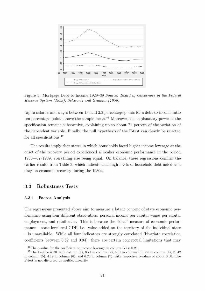
Having examined the debt ratios at the onset of the Great Depression, I now turnto the debt overhang households continued to face in 1932. This accounts for possiblechanges in household debt-to-income ratios that took place during the contraction pe-riod 1929—32. Figure 5 summarizes the changes in household debt-to-income ratios ingraphical form. Throughout the economic downturn, i.e. from 1929 to 1932, the averagestate-level mortgage debt-to-income ratio slightly increased. This applies both to high-and low-debt states. Yet though income leverage in low-debt states barely increased be-tween 1929 and 1932, income leverage in high-debt states rose by about 11 percentagepoints. Not surprisingly, this indicates that households were unable to repair their balancesheets during the years of contraction; the truth was they faced persistent high or evensignificantly increased debt levels at the onset of the recovery.45

Table 4 assesses the implications of the debt overhang with which households enteredthe period of recovery by regressing the debt-to-income ratio as of 1932 (DEBTs,1932)on the percentage change in economic indicators from 1933 to 1937 and from 1933 to1939. The results are consistent with patterns seen previously when using debt levelsas of 1929. The coefficients on income leverage remain negative and highly significant,which suggests a decrease in the growth rate of employment, per capita income, and per

44Coefficients on MANs,1929 and AGRICs,1929 differ remarkably between income p.c. and salariesand wages p.c. Total personal income p.c. also includes farm and nonfarm proprietor income. (In1929, proprietor income accounted for about 17 percent of total personal income, with farm proprietorincome accounting for seven percent of total personal income and nonfarm proprietor income accountingfor ten percent of total personal income.) In the agricultural sector, farm proprietor income increasesfar more during the period of recovery than do salaries and wages in the farm sector. This impliesthat AGRICs,1929 has a more pronounced effect on income p.c. compared with wages and salaries p.c.For manufacturing, it is impossible to disentangle these dynamics because Schwartz and Graham (1956)report salaries and wages in the manufacturing sector but not proprietor income in the manufacturingsector. I assume that comparable dynamics created the differences in magnitude to the coefficients onMANs,1929.

45As can be expected, there is a strong correlation (0.99) between the mortgage debt-to-income ratioin 1929 and in 1932.

19

Table3:

RegressionResults

Recovery,

1933

–37an

d19

33–3

9(Including

Bou

nce-BackEffe

ct).

(1)

(2)

(3)

(4)

(5)

(6)

(7)

∆INCs

∆W

AGE

s∆

EM

Ps

∆SALESs

∆INCs

∆W

AGE

s∆

EM

Ps

1933

–39

1933

–39

1933

–39

1933–3

919

33–3

719

33–3

719

33–3

7DEBTs ,1929

-0.258

0***

-0.226

6***

-0.3150*

*-0.303

4**

-0.270

8***

-0.284

4***

-0.275

8(0.0837)

(0.074

9)(0.152

0)(0.138

0)(0.098

0)(0.075

6)(0.185

2)

INCs ,1933

-0.040

7-0.060

1**

-0.014

10.08

030.00

680.02

40-0.032

2(0.035

8)(0.023

5)(0.056

2)(0.054

1)(0.039

0)(0.020

53)

(0.056

8)BOUNCEBACK

s-0.322

6**

-0.174

8-1.488

2***

-0.177

4-0.5625*

**-0.353

1***

-1.650

8***

(0.145

3)(0.084

7)(0.412

8)(0.159

5)(0.146

7)(0.113

9)(0.322

6)AGRICs ,1929

2.23

22**

*0.05

26-0.631

0-0.163

41.61

12**

*0.38

30-0.4333

(0.2550)

(0.223

9)(0.547

3)(0.789

1)(0.312

1)(0.388

0)(0.443

7)M

AN

s ,1929

0.20

96*

0.2258

*-0.406

8*-0.128

40.12

580.06

28-0.157

9(0.1292)

(0.127

1)(0.229

5)(0.182

7)(0.154

6)(0.107

5)(0.205

2)NEW

DEALs

0.00

000.00

010.00

020.00

02*

0.00

000.00

010.00

01(0.0001)

(0.000

1)(0.000

1)(0.000

1)(0.000

1)(0.000

1)(0.000

1)M

ONPOLs

-0.2907

-0.027

3**

-0.042

9-0.012

7-0.011

4-0.012

2-0.028

8(0.0179)

(0.013

2)(0.026

5)(0.025

4)(0.016

4)(0.012

0)(0.021

4)Con

stan

t0.2022

**0.30

01**

*0.18

73**

*0.31

610.14

26*

0.21

35**

*0.18

06**

*Sp

ecification

OLS

OLS

OLS

OLS

OLS

OLS

OLS

N48

4948

4848

4846

R2

0.69

520.48

610.47

060.1974

0.68

240.55

440.49

66Note:

Stan

dard

errors

inpa

renthe

ses;

***

p<0.01

,**

p>0.05,

*p<

0.1.

Stan

dard

errors

are

heteroskedasticity-rob

ust.

20

0.0

5.1

.15

.2.2

5.3

.35

1928 1930 1934 1936 19381940 1929 1931 1932 1933 1935 1937 1939Year

Mortgage Debt/Income (Mean) Mortgage Debt/Income (Mean of 13 Low Debt States)

Mortgage Debt/Income (Mean of 13 High Debt States)

Figure 5: Mortgage Debt-to-Income 1929–39 Source: Board of Governors of the FederalReserve System (1959); Schwartz and Graham (1956).

capita salaries and wages between 1.6 and 2.3 percentage points for a debt-to-income ratioten percentage points above the sample mean.46 Moreover, the explanatory power of thespecification remains substantive, explaining up to about 71 percent of the variation ofthe dependent variable. Finally, the null hypothesis of the F-test can clearly be rejectedfor all specifications.47

The results imply that states in which households faced higher income leverage at theonset of the recovery period experienced a weaker economic performance in the period1933—37/1939, everything else being equal. On balance, these regressions confirm theearlier results from Table 3, which indicate that high levels of household debt acted as adrag on economic recovery during the 1930s.

3.3 Robustness Tests

3.3.1 Factor Analysis

The regressions presented above aim to measure a latent concept of state economic per-formance using four different observables: personal income per capita, wages per capita,employment, and retail sales. This is because the “ideal” measure of economic perfor-mance – state-level real GDP, i.e. value added on the territory of the individual state– is unavailable. While all four indicators are strongly correlated (bivariate correlationcoefficients between 0.82 and 0.94), there are certain conceptual limitations that may

46The p-value for the coefficient on income leverage in column (7) is 0.26.47The F-value is 30.02 in column (1), 8.71 in column (2), 5.31 in column (3), 2.6 in column (4), 23.42

in column (5), 4.12 in column (6), and 6.23 in column (7), with respective p-values of about 0.00. TheF-test is not distorted by multicollinearity.

21

Table4:

RegressionResults

Recovery,

1933

–37an

d19

33–3

9(U

sing

DebtLe

vels

asof

1932)

(1)

(2)

(3)

(4)

(5)

(6)

(7)

∆INCs

∆W

AGE

s∆

EM

Ps

∆SALESs

∆INCs

∆W

AGE

s∆

EM

Ps

1933

–39

1933

–39

1933

–39

1933–3

919

33–3

719

33–3

719

33–3

7DEBTs ,1932

-0.197

0***

-0.155

6***

-0.2008*

*-0.224

3**

-0.203

0***

-0.193

4***

-0.156

7(0.0547)

(0.049

7)(0.102

1)(0.092

2)(0.058

3)(0.052

5)(0.134

9)INCs ,1933

-0.032

2-0.057

2**

-0.011

80.09

24*

0.01

530.02

74-0.0356

(0.033

4)(0.023

5)(0.057

2)(0.053

4)(0.038

2)(0.020

6)(0.060

2)BOUNCEBACK

s-0.333

4**

-0.178

1-1.478

5***

-0.190

1-0.5741*

**-0.357

2***

-1.645

6***

(0.141

4)(0.133

0)(0.415

6)(0.158

0)(0.143

2)(0.115

5)(0.330

4)AGRICs ,1929

2.24

70**

*0.06

95-0.617

6-0.157

31.62

57**

*0.40

35-0.4167

(0.2467)

(0.221

3)(0.555

6)(0.773

2)(0.319

3)(0.384

7)(0.457

0)M

AN

s,1929

0.23

56*

0.2356

*-0.404

7*-0.115

80.15

050.07

37-0.161

9(0.1237)

(0.125

5)(0.232

2)(0.176

8)(0.150

5)(0.106

3)(0.208

6)NEW

DEALs

0.00

000.00

010.00

020.00

02*

0.00

000.00

010.00

01(0.0001)

(0.000

1)(0.000

1)(0.000

1)(0.000

1)(0.000

1)(0.000

1)M

ONPOLs

-0.0278

-0.027

0**

-0.043

0-0.011

2-0.010

3-0.011

2-0.029

3(0.0175)

(0.012

8)(0.026

4)(0.024

9)(0.016

1)(0.011

6)(0.021

6)Con

stan

t0.19

07**

*0.29

47**

*0.18

23**

*0.30

31**

*0.13

07**

0.20

69**

*0.17

78**

*Sp

ecification

OLS

OLS

OLS

OLS

OLS

OLS

OLS

N48

4948

4848

4846

R2

0.70

750.49

270.46

790.2135

0.69

400.56

430.49

66Note:

Stan

dard

errors

inpa

renthe

ses;

***

p<0.01

,**

p>0.05,

*p<

0.1.

Stan

dard

errors

are

heteroskedasticity-rob

ust.

22

dilute their quality as proxies for real state-level GDP. Personal income per capita andwages per capita might be biased because they include out-of-state wage earnings as wellas property income from out-of-state assets. The retail sales indicator measures changesof consumption at the state level. Hence, it reflects changes in personal income as wellas changes in the propensity to consume. A further bias might result because retail salesinclude both sales of tradable as well as non-tradable goods, which means they also in-clude goods that have been produced out of state. The employment indicator is only fullyconsistent if we assume that state-level demand for labor derives entirely from the demandfor goods produced within the state. Despite these limitations, however, a substantiveshare of the variance for all four variables can be attributed to state-level fluctuations ofeconomic performance.

One way to estimate how well these indicators record state-level economic performanceis to undertake an explanatory factor analysis. This method identifies the extent towhich the variance of these four measures is caused by a set of common, underlying (orunobservable) factors.

The analysis suggests that one dominant factor – state economic performance – drives90 percent of existing cross-state variance in personal income per capita, wages per capita,employment, and retail sales in the period 1929–39.48 The loading patterns in Table 5(see Appendix) confirm the substantive influence of this factor on all four indicators.Hence, using the factor scores calculated from this analysis as a dependent variable offersan additional way to scrutinize the effect of high levels of household debt on economicperformance so as to examine the robustness of earlier findings.49

3.3.2 Dynamics in Recession and Recovery

The results presented above suggest a statistically significant negative relationship be-tween household indebtedness and economic performance during the period of recovery,i.e. from 1933 to 1937 and from 1933 to 1939, respectively. Yet it is possible that dynamicsdiffer when it comes to recession and recovery. Previous contributions (e.g. Wallis (1989)and Garrett and Wheelock (2006)) point out the important role of industrial structurevariation in determining differences in economic performances during the 1930s. Accord-ing to their findings, adverse economic effects of high levels of household indebtednessmay vary in recession and recovery depending on the significance of other shocks, such asthose affecting the agricultural sector or manufacturing industries. Hence, I use a more

48As data for retail sales is only available for the years 1929, 1933, 1935, and 1939, the analysis is basedon observations for these years. (At that time there were only 48 states.) The corresponding eigenvalue ofthis factor is 3.6, compared with 0.2 for the second (see Appendix, Table 10). For the respective scoringcoefficients, see Table 10 (see the Appendix).

49Summary statistics for the factor score in 1929, 1933, and 1939 are presented in Table 13 (see theAppendix).

23

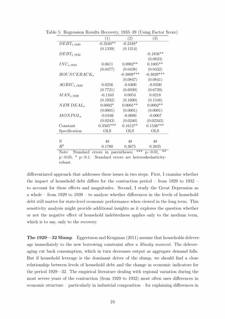
Table 5: Regression Results Recovery, 1933–39 (Using Factor Score)(1) (2) (3)

DEBTs,1929 -0.3240** -0.2348*(0.1339) (0.1214)

DEBTs,1932 -0.1856**(0.0823)

INCs,1933 0.0611 0.0902** 0.1005**(0.0477) (0.0438) (0.0432)

BOUNCEBACKs -0.3809*** -0.3829***(0.0847) (0.0841)

AGRICs,1929 0.0256 -0.0400 -0.0330(0.7721) (0.6939) (0.6739)

MANs,1929 -0.1163 0.0054 0.0218(0.1932) (0.1600) (0.1548)

NEWDEALs 0.0002* 0.0001** 0.0002**(0.0001) (0.0001) (0.0001)

MONPOLs -0.0166 -0.0080 -0.0067(0.0243) (0.0240) (0.02343)

Constant 0.3505*** 0.1612** 0.1536***Specification OLS OLS OLS

N 48 48 48R2 0.1780 0.3675 0.3835Note: Standard errors in parentheses; *** p<0.01, **p>0.05, * p<0.1. Standard errors are heteroskedasticity-robust.

differentiated approach that addresses these issues in two steps. First, I examine whetherthe impact of household debt differs for the contraction period – from 1929 to 1932 –to account for these effects and magnitudes. Second, I study the Great Depression asa whole – from 1929 to 1939 – to analyze whether differences in the levels of householddebt still matter for state-level economic performance when viewed in the long term. Thissensitivity analysis might provide additional insights as it explores the question whetheror not the negative effect of household indebtedness applies only to the medium term,which is to say, only to the recovery.

The 1929—32 Slump Eggertsson and Krugman (2011) assume that households delever-age immediately to the new borrowing constraint after a Minsky moment. The delever-aging cut back consumption, which in turn decreases output as aggregate demand falls.But if household leverage is the dominant driver of the slump, we should find a closerelationship between levels of household debt and the change in economic indicators forthe period 1929—32. The empirical literature dealing with regional variation during themost severe years of the contraction (from 1929 to 1932) most often uses differences ineconomic structure – particularly in industrial composition – for explaining differences in

24

economic performance (see for example Wallis (1989)). According to Garrett and Whee-lock (2006, 464), for example, states that derived a high percentage of personal incomefrom sectors facing severe shocks50 during the contraction years experienced larger de-clines in per capita income than did more diversified states or states depending mainlyon sectors that performed comparably well during the slump.

For the contraction phase, the specification is slightly altered. NEWDEALs wasomitted because New Deal spending did not start until 1933. Instead, the specificationincludes BANKFAILs because the series of four banking panics identified by Friedmanand Schwartz (1963) began in fall 1930 and only ended with Roosevelt’s banking holidayin March 1933. The initial prosperity is defined as state-level income per capita as a shareof total U.S. income p.c. in 1929 (INCs,1929).

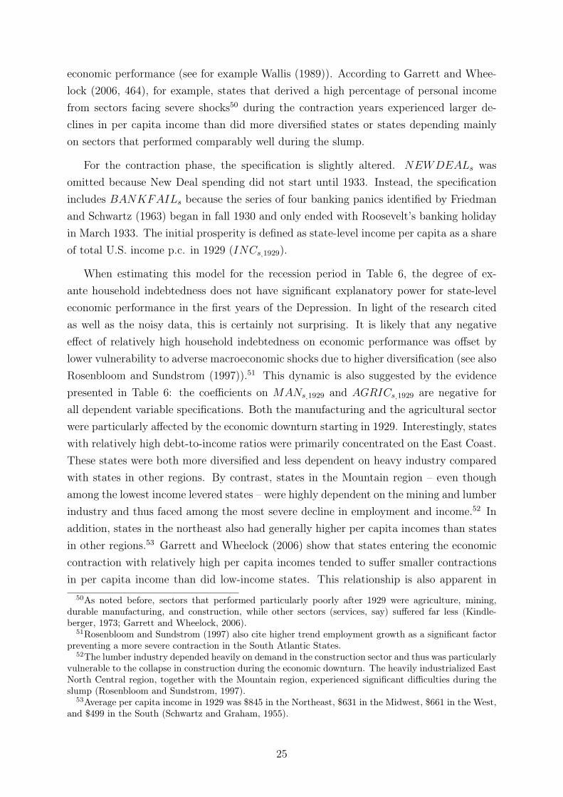
When estimating this model for the recession period in Table 6, the degree of ex-ante household indebtedness does not have significant explanatory power for state-leveleconomic performance in the first years of the Depression. In light of the research citedas well as the noisy data, this is certainly not surprising. It is likely that any negativeeffect of relatively high household indebtedness on economic performance was offset bylower vulnerability to adverse macroeconomic shocks due to higher diversification (see alsoRosenbloom and Sundstrom (1997)).51 This dynamic is also suggested by the evidencepresented in Table 6: the coefficients on MANs,1929 and AGRICs,1929 are negative forall dependent variable specifications. Both the manufacturing and the agricultural sectorwere particularly affected by the economic downturn starting in 1929. Interestingly, stateswith relatively high debt-to-income ratios were primarily concentrated on the East Coast.These states were both more diversified and less dependent on heavy industry comparedwith states in other regions. By contrast, states in the Mountain region – even thoughamong the lowest income levered states – were highly dependent on the mining and lumberindustry and thus faced among the most severe decline in employment and income.52 Inaddition, states in the northeast also had generally higher per capita incomes than statesin other regions.53 Garrett and Wheelock (2006) show that states entering the economiccontraction with relatively high per capita incomes tended to suffer smaller contractionsin per capita income than did low-income states. This relationship is also apparent in

50As noted before, sectors that performed particularly poorly after 1929 were agriculture, mining,durable manufacturing, and construction, while other sectors (services, say) suffered far less (Kindle-berger, 1973; Garrett and Wheelock, 2006).

51Rosenbloom and Sundstrom (1997) also cite higher trend employment growth as a significant factorpreventing a more severe contraction in the South Atlantic States.

52The lumber industry depended heavily on demand in the construction sector and thus was particularlyvulnerable to the collapse in construction during the economic downturn. The heavily industrialized EastNorth Central region, together with the Mountain region, experienced significant difficulties during theslump (Rosenbloom and Sundstrom, 1997).

53Average per capita income in 1929 was $845 in the Northeast, $631 in the Midwest, $661 in the West,and $499 in the South (Schwartz and Graham, 1955).

25

column (1) and (2). The results suggest that states with high per capita incomes as of1929 performed better when compared with states that had lower levels of per capitaincome.

Table 6: Regression Results Contraction, 1929–32(1) (2) (3)

∆ INCs 1929–32 ∆ SALs 1929–32 ∆ EMPs 1931–32DEBTs,1929 0.0980 0.0624 0.1592

(0.1508) (0.1235) (0.0963)INCs,1929 0.1508** 0.0942* -0.0164

(0.0610) (0.0551) (0.02815)AGRICs,1929 -0.7673* -0.0215 -0.4437

(0.4600) (0.4671) (0.4995)MANs,1929 -0.2011 -0.5631** -0.0240

(0.2259) (0.2263) (0.1343)BANKFAILs -0.3001* -0.0597 0.1653

(0.1757) (0.1635) (0.1197)MONPOLs -0.0035 0.0128 0.0116

(0.0241) (0.0222) (0.0166)Constant -0.3910*** -0.2416*** -0.1010***Specification OLS OLS OLS

N 49 48 47R2 0.4312 0.2580 0.1362Note: Standard errors in parentheses; *** p<0.01, ** p>0.05, * p<0.1.Standard errors are heteroskedasticity-robust.

The Great Depression, 1929–39 The results so far indicate the important role ofdebt overhang in the recovery, but not in the slump period. Highly indebted statesrecovered more slowly but did not suffer from a worse recession. The natural next stepis to look at the entire Great Depression episode. Reassuringly, the detrimental effects ofdebt overhang become clearly visibly once the time frame is enlarged.

Table 7 regresses DEBTs,1929 on the percentage change in the four indicators of eco-nomic performance: income per capita, salaries and wages per capita, employment, andconsumption on ex-ante household indebtedness.54 Seven separate estimations ((1)-(7))are reported. Regressions over 1929–39 and 1929–37 produce essentially similar results.In all cases, the coefficients on the key regressor of interest – household debt – show the

54The model controls for both BANKFAILs and NEWDEALs since the period covers the series ofbanking panics between 1930 and 1933 as well as the years of the New Deal. Just as in Table 6 for thecontraction phase, initial prosperity is defined as income per capita at the state level in 1929 as the shareof total U.S. income p.c. in 1929 (INCs,1929). For percentage change in employment, the model is slightlyaltered due to data specifics (see column (3)). The employment index by Wallis (1989), though it startsin 1929, uses only state-level data from 1931 on. Before 1931, the indices are based on regional data.This means that state-level estimates reflect differences in the composition of employment regarding theshare of nonmanufacturing and manufacturing employment; they do not reflect specific state-level trends.

26

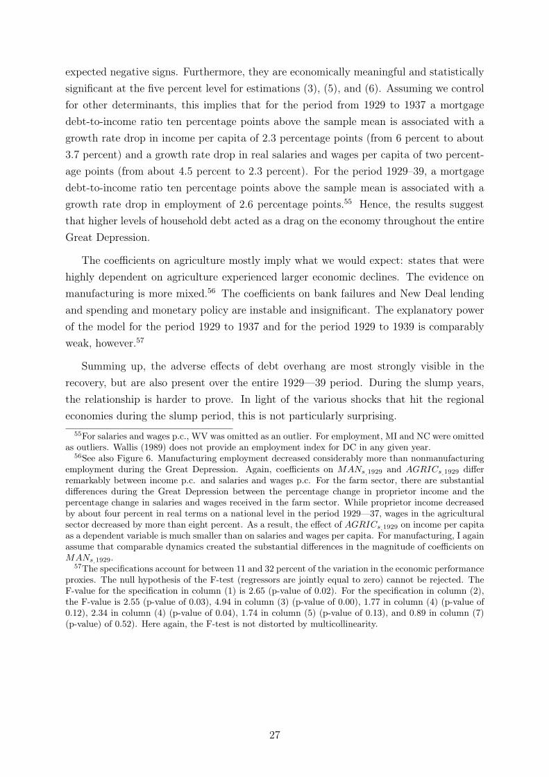
expected negative signs. Furthermore, they are economically meaningful and statisticallysignificant at the five percent level for estimations (3), (5), and (6). Assuming we controlfor other determinants, this implies that for the period from 1929 to 1937 a mortgagedebt-to-income ratio ten percentage points above the sample mean is associated with agrowth rate drop in income per capita of 2.3 percentage points (from 6 percent to about3.7 percent) and a growth rate drop in real salaries and wages per capita of two percent-age points (from about 4.5 percent to 2.3 percent). For the period 1929–39, a mortgagedebt-to-income ratio ten percentage points above the sample mean is associated with agrowth rate drop in employment of 2.6 percentage points.55 Hence, the results suggestthat higher levels of household debt acted as a drag on the economy throughout the entireGreat Depression.

The coefficients on agriculture mostly imply what we would expect: states that werehighly dependent on agriculture experienced larger economic declines. The evidence onmanufacturing is more mixed.56 The coefficients on bank failures and New Deal lendingand spending and monetary policy are instable and insignificant. The explanatory powerof the model for the period 1929 to 1937 and for the period 1929 to 1939 is comparablyweak, however.57

Summing up, the adverse effects of debt overhang are most strongly visible in therecovery, but are also present over the entire 1929—39 period. During the slump years,the relationship is harder to prove. In light of the various shocks that hit the regionaleconomies during the slump period, this is not particularly surprising.

55For salaries and wages p.c., WV was omitted as an outlier. For employment, MI and NC were omittedas outliers. Wallis (1989) does not provide an employment index for DC in any given year.

56See also Figure 6. Manufacturing employment decreased considerably more than nonmanufacturingemployment during the Great Depression. Again, coefficients on MANs,1929 and AGRICs,1929 differremarkably between income p.c. and salaries and wages p.c. For the farm sector, there are substantialdifferences during the Great Depression between the percentage change in proprietor income and thepercentage change in salaries and wages received in the farm sector. While proprietor income decreasedby about four percent in real terms on a national level in the period 1929—37, wages in the agriculturalsector decreased by more than eight percent. As a result, the effect of AGRICs,1929 on income per capitaas a dependent variable is much smaller than on salaries and wages per capita. For manufacturing, I againassume that comparable dynamics created the substantial differences in the magnitude of coefficients onMANs,1929.

57The specifications account for between 11 and 32 percent of the variation in the economic performanceproxies. The null hypothesis of the F-test (regressors are jointly equal to zero) cannot be rejected. TheF-value for the specification in column (1) is 2.65 (p-value of 0.02). For the specification in column (2),the F-value is 2.55 (p-value of 0.03), 4.94 in column (3) (p-value of 0.00), 1.77 in column (4) (p-value of0.12), 2.34 in column (4) (p-value of 0.04), 1.74 in column (5) (p-value of 0.13), and 0.89 in column (7)(p-value) of 0.52). Here again, the F-test is not distorted by multicollinearity.

27

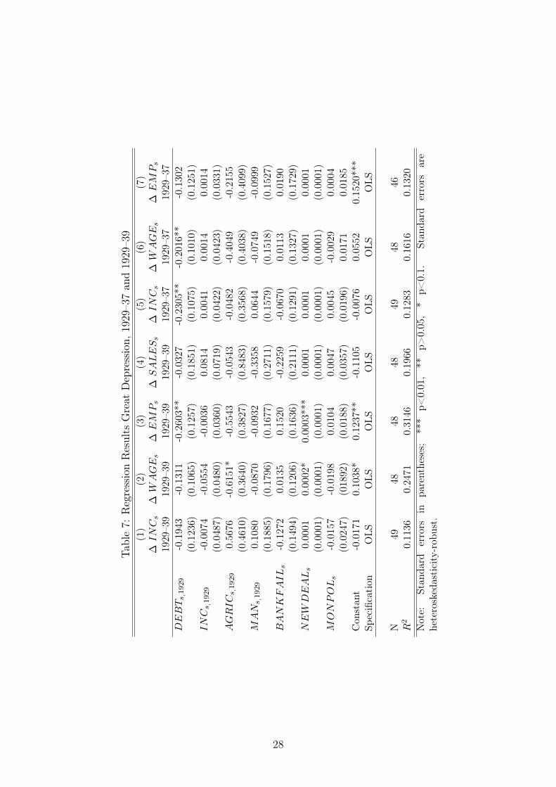
Table7:

RegressionResults

Great

Depression,

1929

–37an

d19

29–3

9(1)

(2)

(3)

(4)

(5)

(6)

(7)

∆INCs

∆W

AGE

s∆

EM

Ps

∆SALESs

∆INCs

∆W

AGE

s∆

EM

Ps

1929

–39

1929

–39

1929

–39

1929

–39

1929

–37

1929

–37

1929

–37

DEBTs ,1929

-0.194

3-0.131

1-0.260

3**

-0.032

7-0.2305*

*-0.201

6**

-0.130

2(0.123

6)(0.106

5)(0.125

7)(0.185

1)(0.107

5)(0.101

0)(0.125

1)INCs ,1929

-0.007

4-0.055

4-0.003

60.08

140.0041

0.00

140.00

14(0.048

7)(0.048

0)(0.036

0)(0.071

9)(0.042

2)(0.042

3)(0.033

1)AGRICs ,1929

0.56

76-0.615

1*-0.554

3-0.054

3-0.048

2-0.404

9-0.215

5(0.461

0)(0.364

0)(0.382

7)(0.848

3)(0.356

8)(0.403

8)(0.409

9)M

AN

s ,1929

0.10

80-0.087

0-0.093

2-0.335

80.06

44-0.074

9-0.099

9(0.188

5)(0.179

6)(0.167

7)(0.271

1)(0.157

9)(0.151

8)(0.152

7)BANKFAILs

-0.127

20.01

350.15

20-0.225

9-0.067

00.01

130.01

90(0.149

4)(0.120

6)(0.163

6)(0.211

1)(0.129

1)(0.132

7)(0.172

9)NEW

DEALs

0.00

010.00

02*

0.0003

***

0.00

010.00

010.00

010.00

01(0.000

1)(0.000

1)(0.000

1)(0.000

1)(0.000

1)(0.000

1)(0.000

1)M

ONPOLs

-0.015

7-0.019

80.01

040.00

470.00

45-0.002

90.00

04(0.024

7)(018

92)

(0.0188)

(0.035

7)(0.019

6)0.0171

0.01

85Con

stan

t-0.017

10.10

38*

0.12

37**

-0.110

5-0.007

60.05

520.15

20**

*Sp

ecification

OLS

OLS

OLS

OLS

OLS

OLS

OLS

N49

4848

4849

4846

R2

0.11

360.24

710.31

460.19

660.12

830.16

160.13

20Note:

Stan

dard

errors

inpa

renthe

ses;

***

p<0.01

,**

p>0.05,

*p<

0.1.

Stan

dard

errors

are

heteroskedasticity-rob

ust.

28

3.4 Deleveraging in the 1930s

The previous subsections have revealed an important feature of the recovery from theU.S. Great Depression. High debt balances in the household sector had an adverse effecton state economic performance. This was predominantly a recovery effect. Can we saysomething about the particular channels through which high household debt held backthe economy?

Eggertsson and Krugman (2011) and Guerrieri and Lorenzoni (2011) propose that inresponse to the deleveraging shock – the sudden downward revision of acceptable debtlevels – households decrease indebtedness to arrive at the new borrowing constraint. Ac-cording to the theoretical and empirical studies discussed in section 2, an important aspectin the process of deleveraging is a decline in consumption, as households are forced tocut back on expenditures to repair their balance sheets (see also Mian et al. (2011)).For the period of the Great Depression, several authors documented a strong decrease inconsumption (for example, Romer (1993) and Olney (1999)). Moreover, Mishkin (1978)argued that household debt had an important role in explaining the consumption col-lapse during the 1930s. The evidence presented in the previous subsections also providessuggestive evidence for a negative relationship between high initial debt levels and thegrowth rates in retail sales between 1933 and 1939. This negative relationship suggeststhat consumption was weaker in high-income leveraged households during this period. Inthis section, I explore deleveraging as a potential channel in greater detail.

The immediate question is whether high debt-to-income states reduced their indebt-edness more during the period of recovery. The assumption that deleveraging may bean important transmission mechanism implies that states with higher pre-recession debtratios deleverage more when adjusting to their targeted net debt position in response toan economic crisis. Figure 5 already provides a first indication. Between 1933 and 1937,the average state-level mortgage debt-to-income ratio dropped by about 50 percent. Yetthe dynamics were substantively different between states with high household debt ratiosand states with lower household debt ratios, particularly during the recovery, Between1932 and 1937, the mortgage debt-to-income ratio fell by 13 percentage points in the 13states with the highest debt-to-income ratios in the sample but only by two percentagepoints in the 13 states with the lowest debt-to-income ratios in the sample.

Table 8 takes a more formal approach by regressing DEBTs,1932 on the change in realmortgage debt per capita (DELEVs) for the two periods of recovery examined earlier,1933—37 and 1933—39.58 The results confirm what Figure 5 intimates: highly indebtedhouseholds reduced debt more aggressively than low-income levered households. Regres-

58DELEVs is defined as lnDEBTs,1937 − lnDEBTs,1933 or lnDEBTs,1939 − lnDEBTs,1933. respec-tively.

29

sion coefficients on debt to income are negative and statistically significant on the five(column (1)) and one percent level (column (2)), respectively. For the period 1933 to1937, the coefficient in column (1) implies a 5.5 percentage point lower growth rate of percapita mortgage debt (from -9 percent to about -15 percent) for a 1932 debt-to-incomeratio ten percentage points above the sample mean. This variation across states in thereduction of debt is pronounced. Between 1933 and 1937, the 13 states with the highestdebt-to-income ratios significantly reduced their per capita mortgage debt stock in realterms by 30 percent. By contrast, the amount of per capita mortgage debt only decreasedby about 6 percent in the 13 states that had the lowest debt-to-income ratios at the on-set of the recovery.59 On balance, the findings provide some support for the theory thatindebted households need to deleverage significantly if they are to repair their balancesheets.60

Table 8: Debt and Deleveraging(1) (2)

∆ DELEVs 1933–37 ∆ DELEVs 1933–39DEBTs,1932 -0.5507** -1.0506***

(0.2284) (0.3045)Constant -0.0214 0.2288***Specification OLS OLS

N 49 49R2 0.1100 0.2020

‚

4 Conclusion

Using U.S. state-level data, this paper examines the relationship between variation in lev-els of household debt and economic performance during the 1930s. The evidence suggeststhat high debt levels were associated with worse economic performance, as recovery wasconsiderably weaker in states with high initial debt-to-income ratios. Everything else be-ing equal, the total growth rate of per capita income, per capita wages, and employmentwas between 2.2 and 3.2 percentage points lower when the household debt-to-income ra-tios were ten percentage points higher than the U.S. average. These results are robust

59The 13 bottom quartile debt-to-income ratio states are CO, FL, ID, IL, MT, NC, NE, NM, OK, PA,SC, TX, and WY; the 13 top quartile debt-to-income ratio states are CA, CT, DE, MA, ME, MI, NH,NJ, NY, RI, UT, and VT.

60For a comprehensive survey of studies contributing to the balance sheet recession view, see Konczal(2012) for. Table 15 (Appendix) shows the regression results for the period 1933-–37 and 1933—39when substituting DEBTs,1929 and DEBTs,1932 with DELEVs as the key explanatory variable. Thecoefficients on deleveraging are positive and statistically significant except for employment in column (7).The model has relatively high explanatory power. It explains between 23 and 69 percent of the variationin real outcomes. These regressions provide suggestive evidence for the fact that the more households ina state reduced their p.c. debt burdens, the weaker the state performed economically.

30

to the inclusion of various controls as well as for different time periods. I interpret thisas evidence that debt overhang created a significant drag for the recovery. Deleveragingof households appears to be an important force driving this trend, as states with higherinitial debt-to-income levels reduced debt at a higher rate. Moreover, though the adverseeffects of high household indebtedness are strongest for the recovery years, they are alsopresent over the entire Depression period 1929–39.

These findings for the Great Depression in the U.S. are consistent with other studiesrelying on cross-sectional variation in household leverage such as Mian et al. (2011) forthe U.S. or King (1994) and the International Monetary Fund (2012) for internationalcontexts. The similarity of the results for very different periods of crisis suggests a closelink between the accumulation of household indebtedness and economic recovery paths.

31

References

Allen, F. L. (1931): Only Yesterday: An Informal History of the Nineteen-Twenties,Blue Ribbon Books, New York.

Bank of Governors of the Federal Reserve System (1943): Banking and Mon-etary Statistics, 1914-1941, Washington, D.C.

Bernanke, B. S. (1983): “Nonmonetary Effects of the Banking Crisis in the Propaga-tionof the Great Depression,” American Economic Review, 70, 257–76.

Board of Governors of the Federal Reserve System (1959): All Bank Statistics1896 - 1955, Washington, D.C.

Bordo, M. D. and J. G. Haubrich (2010): “Credit Crises, Money, and Contractions:A Historical View,” Journal of Monetary Economics, 57, 1–18.

——— (2012): “Deep Recessions, Fast Recoveries, and Financial Crises: Evidence fromthe American Record,” Federal Reserve Bank of Cleveland Working Paper 12-14.

Brunnermeier, M. K. and Y. Sannikov (2012): “Redistributive Monetary Policy,”Jackson Hole Symposium - Federal Reserve Bank of Kansas.

Calomiris, C. W. and J. R. Mason (2003): “Consequences of Bank Distress duringthe Great Depression,” The American Economic Review, 93, 937–947.

Carter, S. B. (2006): Historical Statistics of the United States Millennial Edition On-line, New York: Cambridge University Press, New York, chap. National income, byindustry group: 1929-2002, Tables Ca35-53.

Cerra, V. and S. C. Saxena (2005a): “Did Output Recover from the Asian Crisis?”IMF Staff Papers, 52, 1–23.

——— (2005b): “Eurosclerosis or Financial Collapse: Why Did Swedish Incomes FallBehind?” International Monetary Fund Working Paper.

——— (2008): “Growth Dynamics: The Myth of Economic Recovery,” American EconmicReview, 98, 439–457.

Creamer, D. and C. Merwin (July 1942): “State Distribution of Income Payments1929-41,” Survey of Current Business, 18–26.

Dynan, K. (2012): “Is a Household Debt Overhang Holding Back Consumption?” Brook-ings Papers on Economic Activity.

32

Eggertsson, G. and P. Krugman (2011): “Debt, Deleveraging, and the LiquidityTrap: A Fisher-Minsky-Koo Approach,” Federal Reserve Bank of New York, Unpub-lished Manuscript.

Federal Reserve Board (1933): Ninetheenth Annual Report of the Federal ReserveBoard Covering Operations for the Year 1932, United States Government Printing Of-fice, Washington, D.C.

Fishback, P. V., W. C. Horrace, and S. Kantor (2005): “Did New Deal GrantPrograms Stimulate Local Economies? A Study of Federal Grants and Retail Salesduring the Great Depression,” The Journal of Economic History, 65, 36–71.

Fishback, P. V., S. Kantor, and J. J. Wallis (2003): “Can the New Deal’s Three RsBe Rehabilitated? A Program-by-Program, County-by-County Analysis,” Explorationsin Economic History, 40, 278—307.

Fisher, I. (1933): “The Debt-Deflation Theory of the Great Depression,” Econometrica,1, 337–357.

Friedman, M. (1993): “The "Plucking Model" of Business Fluctuations Revisited,”Economic Inquiry, 31, 171–177.

Friedman, M. and A. J. Schwartz (1963): A Monetary History of the United States,1867-1963., Princeton University Press, Princeton, NJ.

Garrett, T. A. and D. C. Wheelock (2006): “Why Did Income Growth Vary acrossStates during the Great Depression?” The Journal of Economic History, 66, 456–466.

Glick, R. and K. J. Lansing (2009): “U.S. Household Deleveraging and Future Con-sumption Growth,” FRBSF Economic Letter.

——— (2010): “Global Household Leverage, House Prices, and Consumption,” FRBSFEconomic Letter.

Goldsmith, R. W. (1955): A Study of Saving in the United States, vol. 1: Introduction;Tables of Annual Estimates of Saving 1897-1949, Greenwood Press Publishers, NewYork.

Grebler, L., D. M. Blank, and L. Winnick (1956): Capital Formation in ResidentialReal Estate: Trends and Prospects, Princeton University Press, Princeton, NJ.

Guerrieri, V. and G. Lorenzoni (2011): “Credit Crises, Precautionary Savings, andthe Liquidity Trap,” Working Paper 17583, National Bureau of Economic Research.

33

Haines, M. R. (2006): Historical Statistics of the United States, Earliest Times to thePresent: Millennial Edition, Cambridge University Press, New York, chap. Populationby race, sex, age, nativity, and urban rural residence, Tables Aa2244-6550.

Hall, R. E. (2011): “The Long Slump,” American Econmic Review, 101, 431–469.

Howard, G., R. Martin, and B. A. Wilson (2011): “Are Recoveries from Bankingand Financial Crises Really So Different?” Board of Governors of the Federal ReserveSystem International Finance Discussion Papers.

Hyman, L. (2011): Debtor Nation: The History of America in Red Ink, Princeton Uni-versity Press, Princeton, NJ.

International Monetary Fund (2009): World Economic Outlook: Crisis and Recov-ery, World Economic and Financial Surveys, International Monetary Fund, Washing-ton, D.C.

——— (2012): World Economic Outlook: Growth Resuming, Dangers Remain, WorldEconomic and Financial Surveys, International Monetary Fund, Washington, D.C.

James, J. A. and R. Sylla (2006): Historical Statistics of the United States, EarliestTimes to the Present: Millennial Edition, Cambridge University Press, New York, chap.Net public and private debt, by major sector: 1916–1976, Tables Cj875–889.

Kaminsky, G. L. and C. M. Reinhart (1999): “The Twin Crises: The Causes ofBanking and Balance-Of-Payments Problems,” The American Economic Review, 89,473–500.

Kindleberger, C. P. (1973): The World in Depression, 1929-1939, London.

King, M. (1994): “Debt Deflation: Theory and Evidence,” European Economic Review,38, 419–445.

Konczal, M. (2012): “How Mortgage Debt is Holding Back the Recovery,” Tech. rep.,The Roosevelt Institute.

Krugman, P. (2012): “1933 and All That,” The Conscience of a Liberal [blog entry],New York Times.

Margo, R. A. (1993): “Employment and Unemployment in the 1930s,” Journal of Eco-nomic Perspectives, 7, 41–59.

Mian, A. and A. Sufi (2009): “Household Leverage and the Recession of 2007 to 2009,”University of Chicago, Booth School of Business Working Paper.

34

Mian, A. R., K. Rao, and A. Sufi (2011): “Household Balance Sheets, Consumption,and the Economic Slump,” Unpublished Working Paper.

Mian, A. R. and A. Sufi (2012): “What Explains High Unemployment? The AggregateDemand Channel,” NBER Working Paper 17830.

Minsky, H. (1986): Stabilizing an Unstable Economy, Yale University Press, New Haven,CT.

Mishkin, F. (1977): “What Depressed the Consumer? The Household Balance Sheetand the 1973-75 Recession,” Brookings Papers on Economic Activity, 123–164.

——— (1978): “The Household Balance Sheet and the Great Depression,” Journal ofEconomic History, 38, 918–937.

Olney, M. L. (1987): “Advertising, Consumer Credit, and the ’Consumer DurablesRevolution’ of the 1920s,” The Journal of Economic History, 47, 489–491.

——— (1999): “Avoiding Default: The Role of Credit in the Consumption Collapse of1930,” The Quarterly Journal of Economics, 114, 319–335.

Palley, T. I. (1994): “Debt, Aggregate Demand, and the Business Cycle: An Analysis inthe Spirit of Kaldor and Minsky,” Journal of Post Keynesian Economics, 16, 371–390.

Philippon, T. and V. Midrigan (2011): “Household Leverage and the Recession,”NBER Working Paper 16965.

Reinhart, C. M. and V. R. Reinhart (2010): “After the Fall,” NBER Working Paper16334.

Reinhart, C. M. and K. S. Rogoff (2009a): “The Aftermath of Financial Crises,”NBER Working Paper 14656.

——— (2009b): This Time Is Different: Eight Centuries of Financial Folly, PrincetonUniversity Press, Princeton, NJ.

——— (2012): “This Time is Different, Again? The US Five Years after the Onset ofSubprime,” Voxeu.org.

Rockoff, H. (1998): The Defining Moment. The Great Depression and the AmericanEconomy in the Twentieth Century, The University of Chicago Press, Chicago, chap.By Way of Analogy: The Expansion of the Federal Government in the 1930s.

Romer, C. D. (1990): “The Great Crash and the Onset of the Great Depression,” TheQuarterly Journal of Economics, 105, 597–624.

35

——— (1992): “What Ended the Great Depression?” Journal of Economic History, 52,757–784.

——— (1993): “The Nation in Depression,” Journal of Economic Perspectives, 7, 19–39.

Rosenbloom, J. L. and W. A. Sundstrom (1997): “The Sources of Regional Variationin the Severity of the Great Depression: Evidence from U.S. Manufacturing, 1919-1937,”NBER Working Paper 6288.

Schularick, M. and A. M. Taylor (2012a): “Credit Booms Gone Bust: MonetaryPolicy, Leverage Cycles, and Financial Crises 1870-2008,” American Economic Review,102, 1029–1061.

——— (2012b): “Fact-Checking Financial Recessions: US-UK Update,” Voxeu.org.

Schwartz, C. F. and R. E. Graham (1955): “Personal Income by States, 1929—54,”Survey of Current Business.

——— (1956): Personal Income by States Since 1929: A Supplement to the Survey ofCurrent Business., Greenwood Press Publishers, New York.

Sutherland, D., P. Hoeller, R. Merola, and V. Zieman (2012): “Debt andMacroeconomic Stability,” OECD Economics Department Working Paper 1003.

Taylor, A. M. (2012): “The Great Leveraging,” NBER Working Paper 18290.

Temin, P. (1976): Did Monetary Forces Cause the Great Depression?, W.W. Norton &Company, New York.

Tobin, J. (1980): Asset Accumulation and Economic Activity: Reflections on Contem-porary Macroeconomic Theory, The University of Chicago Press, Chicago, IL.

——— (1989): “Review of ’Stabilizing an Unstable Economy’ by Hyman P. Minsky,”Journal of Economic Literature, 27, 105–108.

U.S. Bureau of the Census (various years): “Current Population Reports. Series P-25,Population Estimates and Projections. Nos. 311, 917, 1095,” Series P-25, Populationestimates and projections. Nos. 311, 917, 1095.

U.S. Department of Labor: Bureau of Labor Statistics (2012): “ConsumerPrice Index for All Urban Consumers: All Items,” Federal Reserve Bank of St. Louis.

Vatter, H. G. (1967): “Has There Been A Twentieth-Century Consumer Durables Rev-olution?” The Journal of Economic History, 27, 1–16.

36

Wallis, J. J. (1989): “Employment in the Great Depression: New Data and Hypotheses,”Explorations in Economic History, 26, 45–72.

White, E. N. (2009): “Lessons from the Great American Real Estate Boom and Bust ofthe 1920s,” Working Paper 15573, National Bureau of Economic Research.

37

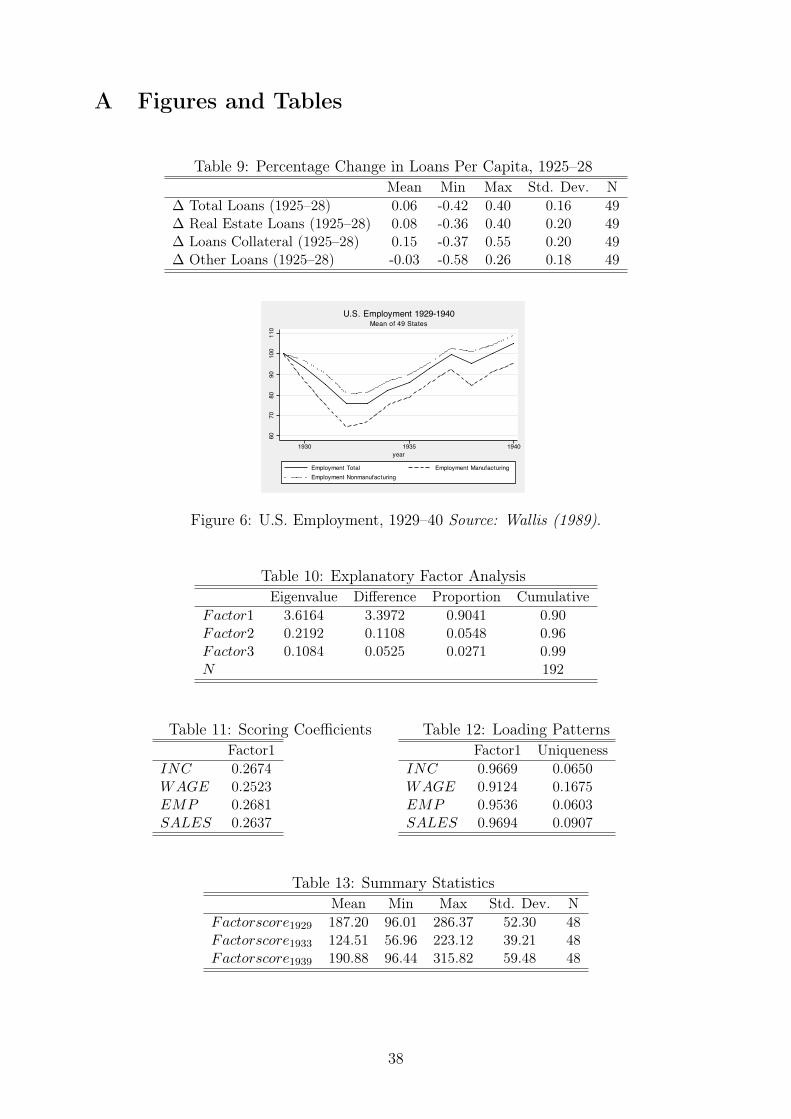
A Figures and Tables

Table 9: Percentage Change in Loans Per Capita, 1925–28Mean Min Max Std. Dev. N

∆ Total Loans (1925–28) 0.06 -0.42 0.40 0.16 49∆ Real Estate Loans (1925–28) 0.08 -0.36 0.40 0.20 49∆ Loans Collateral (1925–28) 0.15 -0.37 0.55 0.20 49∆ Other Loans (1925–28) -0.03 -0.58 0.26 0.18 49

6070

8090

100

110

1930 1935 1940year

Employment Total Employment ManufacturingEmployment Nonmanufacturing

Mean of 49 StatesU.S. Employment 1929-1940

Figure 6: U.S. Employment, 1929–40 Source: Wallis (1989).

Table 10: Explanatory Factor AnalysisEigenvalue Difference Proportion Cumulative

Factor1 3.6164 3.3972 0.9041 0.90Factor2 0.2192 0.1108 0.0548 0.96Factor3 0.1084 0.0525 0.0271 0.99N 192

Table 11: Scoring CoefficientsFactor1

INC 0.2674WAGE 0.2523EMP 0.2681SALES 0.2637

Table 12: Loading PatternsFactor1 Uniqueness

INC 0.9669 0.0650WAGE 0.9124 0.1675EMP 0.9536 0.0603SALES 0.9694 0.0907

Table 13: Summary StatisticsMean Min Max Std. Dev. N

Factorscore1929 187.20 96.01 286.37 52.30 48Factorscore1933 124.51 56.96 223.12 39.21 48Factorscore1939 190.88 96.44 315.82 59.48 48

38

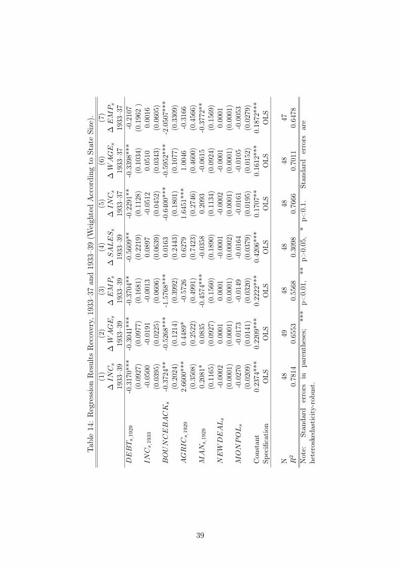
Table14

:RegressionResults

Recovery,

1933

–37an

d19

33–3

9(W

eigh

tedAccording

toStateSize).

(1)

(2)

(3)

(4)

(5)

(6)

(7)

∆INCs

∆W

AGE

s∆

EM

Ps

∆SALESs

∆INCs

∆W

AGE

s∆

EM

Ps

1933

–39

1933

–39

1933

–39

1933–3

919

33–3

719

33–3

719

33–3

7DEBTs ,1929

-0.317

0***

-0.304

1***

-0.3704*

*-0.560

9**

-0.229

1**

-0.339

8***

-0.210

7(0.0927)

(0.097

7)(0.168

1)(0.221

9)(0.112

8)(0.103

4)(0.196

2)

INCs ,1933

-0.050

0-0.019

1-0.001

30.08

97-0.051

20.05

100.00

16(0.039

5)(0.022

5)(0.060

6)(0.063

9)(0.045

2)(0.034

3)(0.060

5)BOUNCEBACK

s-0.372

4**

-0.526

8***

-1.576

8***

0.01

63-0.6400*

**-0.595

2***

-2.050

7***

(0.202

4)(0.121

4)(0.399

2)(0.244

3)(0.180

1)(0.107

7)(0.330

9)AGRICs ,1929

2.66

00**

*0.44

89*

-0.572

60.62

791.64

51**

*1.00

46-0.316

6(0.3508)

(0.252

2)(0.499

1)(0.742

3)(0.274

6)(0.460

0)(0.456

6)M

AN

s ,1929

0.20

81*

0.08

35-0.457

4***

-0.035

80.20

93-0.061

5-0.377

2**

(0.1165)

(0.092

7)(0.156

0)(0.189

0)(0.113

4)(0.092

4)(0.156

9)NEW

DEALs

-0.000

20.00

010.00

01-0.000

1-0.000

2-0.000

10.00

01(0.000

1)(0.000

1)(0.000

1)(0.000

2)(0.000

1)(0.000

1)(0.000

1)M

ONPOLs

-0.027

0-0.017

3-0.014

9-0.016

4-0.016

1-0.010

5-0.005

3(0.020

9)(0.014

1)(0.032

0)(0.037

9)(0.019

5)(0.015

2)(0.027

9)Con

stan

t0.23

74**

*0.22

09**

*0.22

22**

*0.42

06**

*0.17

07**

0.16

12**

*0.18

72**

*Sp

ecification

OLS

OLS

OLS

OLS

OLS

OLS

OLS

N48

4948

4848

4847

R2

0.78

140.65

530.55

680.3098

0.76

660.70

110.64

78Note:

Stan

dard

errors

inpa

renthe

ses;

***

p<0.01

,**

p>0.05,

*p<

0.1.

Stan

dard

errors

are

heteroskedasticity-rob

ust.

39

Table15

:RegressionResults

Recovery,

1933

–37an

d19

33–3

9-Deleverag

ing

(1)

(2)

(3)

(4)

(5)

(6)

(7)

∆INCs

∆W

AGE

s∆

EM

Ps

∆SALESs

∆INCs

∆W

AGE

s∆

EM

Ps

1933

–39

1933

–39

1933

–39

1933

–39

1933

–37

1933

–37

1933

–37

DELEVs

0.08

44**

*0.05

63**

*0.05

48*

0.08

19**

0.08

72*

0.07

02*

0.02

82(0.0249)

(0.018

6)(0.032

8)(0.038

1)(0.051

1)(0.041

1)

(0.042

6)INCs ,1933

-0.054

2-0.074

9-0.063

10.05

67-0.002

1-0.006

5-0.071

7*(0.037

2)(0.027

0)(0.042

4)(0.053

4)(0.044

8)(0.0293)

(0.042

6)BOUNCEBACK

s-0.401

1***

-0.137

8-0.407

7-0.254

6-0.657

3***

-0.248

0**

-1.687

3***

(0.145

8)(0.102

5)(0.327

6)(0.158

6)(0.161

3)(0.1194)

(0.314

4)AGRICs ,1929

2.18

19**

*-0.129

4-0.613

7*-0.212

41.63

56**

*0.10

96-0.360

5(0.245

0)(0.255

8)(0.306

2)(0.643

8)(0.392

6)(0.4020)

(0.501

7)M

AN

s,1929

0.1850

0.18

87-0.114

4-0.148

30.04

270.13

26-0.195

4(0.121

8)(0.092

4)(0.174

3)(0.161

9)(0.145

1)(0.1113)

(0.206

0)NEW

DEALs

-0.000

10.00

010.00

02**

0.00

01-0.000

10.00

000.0000

(0.000

1)(0.000

1)(0.000

1)(0.000

1)(0.000

1)(0.0001)

(0.000

1)M

ONPOLs

-0.037

7**

-0.038

9***

-0.025

9-0.021

9-0.017

3-0.026

0*-0.031

9(0.015

6)(0.013

5)(0.017

5)(0.023

6)(0.015

4)(0.0154)

(0.020

4)Con

stan

t0.1636

**0.30

99**

*0.23

73**

0.27

83**

*0.11

77*

0.20

79**

*0.2921

***

Specification

OLS

OLS

OLS

OLS

OLS

OLS

OLS

N48

4848

4849

4847

R2

0.7249

0.38

630.31

630.22

090.68

060.27

730.46

97Note:

Stan

dard

errors

inpa

renthe

ses;

***

p<0.01

,**

p>0.05

,*

p<0.1.

Stan

dard

errors

are

heteroskedasticity-rob

ust.

40

B Data Appendix

Data on credit has been drawn from Board of Governors of the Federal Reserve System(1959). The All Bank Statistics include statistics on bank balance sheets by bank class andby state for the period 1896-1955, with total loan amounts being recorded on June 30 foreach year (Board of Governors of the Federal Reserve System, 1959, 3). Real estate loansinclude loans on farm land, loans on residential properties, loans on other properties,bonds and mortgages, mortgages purchased, and mortgages owned. When using themortgage debt-to-income ratio, controlling for agricultural states is particularly importantbecause a considerable share of real estate loans might be loans on farm land. Overall,the share of farm mortgages was between 20 and 30 percent of total mortgages duringthe period in which real estate loans were reported in the All Bank Statistics (1925—37).Nevertheless, the real estate loans reported in the All Bank Statistics are a good proxyfor total residential mortgage lending (as discussed in section 3.1). Board of Governorsof the Federal Reserve System (1959) also provide data on loans on collateral and otherloans. Before 1928, loans on collateral include: loans on demand or time secured bystocks and bonds, loans on demand or time secured by other personal securities includingmerchandise, warehouse receipts, etc., loans on securities, loans on demand or time securedby collateral, and loans secured by collateral other than real estate. For the period 1929—38, however, loans on collateral only include loans with securities as collateral. All otherloans include: loans on personal security; loans on depositors’ books; acceptances or billsof exchange purchased or discounted; syndicate participations; customers’ liability onaccount or drafts paid under letters of credit; advances to trust estates; personal loans;commercial paper bought in open market; overdrafts; notes and bills rediscounted loansto banks and trust companies not secured by collateral; loans and discounts not classified.With such a variety of loans, it is difficult to explain why loans in this category mighthave decreased or increased over time.

The federal government did not initiate a monthly survey of the labor force as definedtoday until 1940 (Margo, 1993). Hence, unemployment statistics for the 1930s are notentirely reliable. The employment index as calculated by Wallis (1989) is based on es-tablishment surveys of employment done by the Bureau of Labor Statistics.61 The BLSreported changes in employment over two month periods for firms that reported for bothmonths. This means that the data is biased: it does not include reports of new firms andfirms that stopped operations. To construct a yearly index, Wallis (1989) benchmarkedthe estimated employment changes to known employment totals such as the Census ofManufactures. The author provides three employment indices: total employment, manu-facturing employment, and nonmanufacturing employment. According to the author, the

61Index base year is 1929 (100) (Wallis, 1989).

41

nonmanufacturing index is less reliable than the manufacturing index, as nonmanufac-turing indices had to be approximated while manufacturing employment was collected bythe BLS.

Income data is drawn from the series “Personal Income by States, 1929–1954” reportedin the Survey of Current Business (Schwartz and Graham, 1955). It includes five differentflows of income: i) wage and salary disbursements, ii) other labor income, iii) proprietor’sincome, iv) property income, and v) transfer payments. Wages and salary disbursementsconsist of wages and salaries including compensations of executives, commissions, tips,and bonuses. It covers all payments received in the current period, including retroactivewages. Contributions made by employees for social insurance are deducted from theincome flows. Other labor income covers the following: contributions made by employersto health and welfare funds and private pensions; pay of military reservists; compensationfor injuries; and director’s fees. Proprietor’s income includes the net business earningsfrom owners of noncorporate business both for the farm and nonfarm sector. Propertyincome refers to rental income, cash dividend disbursements by corporations, and personalinterest income. As defined here, rental income measures income received from the rentalof property, royalties on patents, copyrights and rights to natural resources, and net rentalreturns to owner-occupants of nonfarm dwellings. Schwartz and Graham (1956) providesadditional data disaggregating personal income into its components and wages and salariesby industrial sources. Wages and salaries are subdivided into disbursements received fromi) farms, ii) mining, iii) contract construction, iv) manufacturing, v) contract construction,vi) manufacturing, vii) wholesale and retail trade, viii) finance, insurance, and real estate,ix) transportation, x) communication and public utilities, xi) services, xii) government,and xiii) other industries.

Measures of the importance of the manufacturing, agricultural, and construction sectorare calculated as the average annual percentage of personal income received from therespective sector in salary and wage disbursements in 1929. The data is drawn fromSchwartz and Graham (1956).

The degree of bank distress in a state is measured by the annual average rate of banksuspensions in the period 1929—33. Data on the number of bank suspensions are drawnfrom Bank of Governors of the Federal Reserve System (1943, Tables 67, 71, 72); dataon the number of total banks, from Board of Governors of the Federal Reserve System(1959). The term “bank suspension” refers to banks closed to the public both temporarilyor permanently on account of financial difficulties. Suspended banks are closed either bysupervisory authorities or by the banks boards of directors. Banks closed during the bankholiday in 1933 have not been counted as suspensions. Banks that merged with otherbanks without closing are also not counted as suspensions. The same holds for banks thatagreed with depositors to defer the withdrawal of a part of their deposits. Banks that

42

closed and reopened later or were taken over by other institutions after having closed arecounted as suspensions (Bank of Governors of the Federal Reserve System, 1943, 281).

Data on lending and spending of the federal government as part of New Deal pro-grams 1933—39 were drawn from Fishback et al. (2003). The measure used includesNew Deal grants and loans. Grants include Federal Emergency Relief Administrationgrants, Civil Work Administration grants, Works Progress administration grants, PublicAssistance grants provided under the Social Security Act, Public Work Administrationfederal grants, Public Works Administration nonfederal grants, Public Roads Administra-tion grants, Public Buildings Administration grants, Agricultural Adjustment Act grants,Farm Security Administration grants, and U.S. Housing Administration grants. Loans in-clude Public Works Administration nonfederal loans, Farm Credit Administration loans,Rural Electrification Administration loans, Reconstruction Finance Corporation loans,Home Owners Loan Corporation loans, and U.S. Housing Administration loan contracts.For the conversion into per capita grants and loan dollars, data on the population in 1930was used.

County-level data on retail sales were drawn from Fishback et al. (2005) and convertedinto state-level data. For retail sales data for 1933, the authors used the ConsumerMarket Data Handbook as published by the U.S. Department of Commerce in 1936.For retail sales data for 1939, the authors used Historical, Demographic, Economic, andSocial Data: The United States, 1790–1970, ICPSR study number 0003, as corrected byMichael Haines. As there is no data on retail sales in 1937, the period of recovery cannotbe analyzed for consumption as has been done for per capita, salaries and wages percapita, and employment.

Federal Reserve Districts cut across state lines. If a state has two different regionalFederal Reserve Banks, the state is assigned to the District that includes the larger shareof its population (see Federal Reserve Board (1933)). Accordingly, CT is assigned to the1st District; NJ to the 2nd; PA to the 3rd; WV to the 5th; LA and TN to the 6th; IL, IN,MI and WI to the 7th; MS, MO, and KY to the 8th; NM and OK to the 10th; AZ to the12th. Discount rates set by the regional Federal Reserve Banks are drawn from (Bank ofGovernors of the Federal Reserve System, 1943).

For calculating per capita values on debt and income, annual estimates for populationby state were constructed using data drawn from Haines (2006) and U.S. Bureau of theCensus (various years). Haines (2006) provides state-level data on population for thecensus years 1920, 1930, and 1940. U.S. Bureau of the Census (various years) reportsannual national population for the whole period. Combining these two series, the averageannual percentage change in the national data was used for the interpolation of the state-level decadal census data. Even though this data might not cover short-term fluctuations,

43

it provides reliable estimates on general trends of growth or decline in population ona state level. The data was deflated using the Consumer Price Index for All UrbanConsumers (All Items) (U.S. Department of Labor: Bureau of Labor Statistics, 2012). Amajor limitation of the presented state-level analysis is the small number of observations.Nevertheless, it is possible that state-level aggregation masks important local variation.

44

European

Historical

Economics

Society

EHES Working Paper Series

Recent EHES Working Papers

2013

EHES.35

Predicting the Past: Understanding the Causes of Bank Distress in the

Netherlands in the 1920s

Christopher L. Colvin, Abe de Jong and Philip T. Fliers

EHES.34

2012

World Human Development: 1870-2007

Leandro Prados de la Escosura

EHES.33

Farmer Families at the Heart of the Educational Revolution: Which Occupational

Group Inherited Human Capital in the Early Modern Era?

Franziska Tollnek and Joerg Baten

EHES.32

EHES.31

EHES.30

EHES.29

EHES.28

Monetary policy without interest rates. Evidence from France’s Golden Age

(1948-1973) using a narrative approach.

Eric Monnet

Rearmament to the Rescue?

New Estimates of the Impact of ‘Keynesian’ Policies in 1930s’ Britain

Nicholas Crafts and Terence C. Mills

Housing Markets during the Rural-Urban Transition: Evidence from early 20th

Century Spain

Juan Carmona, Markus Lampe and Joan Ramón Rosés

Coping with Regional Inequality in Sweden: Structural Change, Migrations and

Policy, 1860-2000

Kerstin Enflo and Joan Ramón Rosés

Peasant Agriculture and Economic Growth: The Case of Southeast Europe c.

1870-1940 reinterpreted

Michael Kopsidis

All papers may be downloaded free of charge from: www.ehes.org The European Historical Economics Society is concerned with advancing education in European economic

history through study of European economies and economic history. The society is registered with the

Charity Commissioners of England and Wales number: 1052680