IZA DP No. 2976

How Disasters Affect Local Labor Markets:The Effects of Hurricanes in Florida

Ariel R. BelasenSolomon W. Polachek

DI

SC

US

SI

ON

PA

PE

R S

ER

IE

S

Forschungsinstitutzur Zukunft der ArbeitInstitute for the Studyof Labor

August 2007

How Disasters Affect Local Labor Markets:

The Effects of Hurricanes in Florida

Ariel R. Belasen Saint Louis University

Solomon W. Polachek

State University of New York at Binghamton and IZA

Discussion Paper No. 2976 August 2007

IZA

P.O. Box 7240 53072 Bonn

Germany

Phone: +49-228-3894-0 Fax: +49-228-3894-180

E-mail: iza@iza.org

Any opinions expressed here are those of the author(s) and not those of the institute. Research disseminated by IZA may include views on policy, but the institute itself takes no institutional policy positions. The Institute for the Study of Labor (IZA) in Bonn is a local and virtual international research center and a place of communication between science, politics and business. IZA is an independent nonprofit company supported by Deutsche Post World Net. The center is associated with the University of Bonn and offers a stimulating research environment through its research networks, research support, and visitors and doctoral programs. IZA engages in (i) original and internationally competitive research in all fields of labor economics, (ii) development of policy concepts, and (iii) dissemination of research results and concepts to the interested public. IZA Discussion Papers often represent preliminary work and are circulated to encourage discussion. Citation of such a paper should account for its provisional character. A revised version may be available directly from the author.

IZA Discussion Paper No. 2976 August 2007

ABSTRACT

How Disasters Affect Local Labor Markets: The Effects of Hurricanes in Florida*

Exogenous shocks often impact a local labor market more than at the national level. This study improves upon the standard Difference in Difference (DD) approach by examining exogenous shocks using a Generalized Difference in Difference (GDD) econometric approach that identifies the effects of shocks resulting from hurricanes. Based on the Quarterly Census of Employment and Wages (QCEW) data on earnings and employment, the earnings of an average worker in Florida will increase as much as four percent within the first quarter of being hit directly by a hurricane, whereas the effects of a hurricane occurring in a neighboring county move earnings per worker in the opposite direction by roughly the same percentage. As time goes by, workers in both sets of counties will experience faster growth in their earnings than workers in completely unaffected counties; however, this is coupled with a slower growth rate in employment. Powerful hurricanes have greater effects than their weaker counterparts. Additionally, the shifts in earnings and employment can be traced back, in part, to geographic features of the counties, namely that the coastal and Panhandle counties exhibit greater effects than landlocked counties. Although focus is on hurricanes in Florida, this GDD technique is applicable to a wider range of exogenous shocks. JEL Classification: J23, J49, Q54, R11 Keywords: exogenous shock, difference-in-difference estimation, local labor markets,

earnings, employment, hurricanes Corresponding author: Solomon W. Polachek Department of Economics State University of New York at Binghamton Binghamton, New York 13902-6000 USA E-mail: Polachek@binghamton.edu

* All data contained in this paper will be made available upon request. The authors would like to thank Joel Elvery, Christopher Hanes, Kajal Lahiri, and Stan Masters along with the seminar participants at: SUNY Albany; Binghamton University; the Third IZA Migrant Ethnicity Meeting, Washington, D.C. March 2007; and the Twelfth Society of Labor Economists Meetings, Chicago, IL May 2007 for their comments.

1

1. Introduction

An exogenous shock is an unexpected event that impacts a given market. Such shocks can

take many forms, ranging from unexpected new legislation, to sudden population shifts, to domestic

weather-related events, and even to terrorist attacks. A number of studies utilize Difference-in-

Difference (DD) estimation to examine the effects of exogenous shocks. For example, Card (1990)

in a well cited article used DD to examine migration and found relatively small effects on wages.

Such studies look at changes across time periods between the region of interest and a comparable

region which was unaffected by the shock to find long run effects. Angrist and Krueger (1999) call

these results into question for failing to identify an appropriate control group. Perhaps, as a result,

there is now a literature on appropriately choosing control groups, e.g. Bertrand, Duflo, and

Mullainathan (2002), Kubik and Moran (2003), and Abadie, Diamond, and Hainvellen (2007).

Another problem is the experimental group. Most papers examining exogenous shocks rely

on one experimental group; in Card’s (1990) case, this experimental group is Miami, the site of the

Mariel Boatlift. However it is not obvious that one experimental group suffices. In the Card

example, the Miami labor market might not be typical of other potential experimental sites. Perhaps

in his study Miami’s unemployment did not rise because Miami’s economy was growing more

rapidly than other similarly sized cities.

One innovation of this paper is to have many random experimental groups as well as many

random control sites. To achieve this, we use a different natural experiment, hurricanes, to examine

the effect of an exogenous shock on a local labor market. Hurricanes, in particular, are a good

choice for this study because they can affect several counties at a time, and can occur more than

once in the time period under study. By having many experiment sites, we are able to test how the

impact of exogenous shocks differs by both characteristics of the shock and characteristics of the

2

experiment group. Other papers have used weather-related events (e.g. Miguel (2005), Waldman,

Nicholson, and Adilov (2006), and Connolly (2007) all use rainfall) to obtain a purely exogenous

variable as an instrument to predict other independent variables such as how much television

children watch (in the case of Waldman, et al. (2006)), which in turn is used to predict autism using

a simultaneous equation approach. We use weather (i.e. hurricanes) directly as the exogenous

shock we want to evaluate.

To do this, we develop a Generalized Difference-in-Difference (GDD) technique in which

we compare affected regions to unaffected regions across multiple exogenous events and time

periods. In addition, exogenous shocks that are felt positively by one specific labor market can also

have an effect on nearby labor markets. Thus we can examine multiple exogenous shocks affecting

more than one locality at a time. Further, to address the issue of the appropriate definition of

treatment and control group, we compare a given hurricane-stricken county to all other unaffected

counties within that state. In addition, by using quarterly time-series data, this approach has the

advantage of distinguishing short-term and long-term effects that previously had been neglected. In

this way we can better identify the effect of an exogenous shock as well as quantify its effect over

time.

The destructive power of hurricanes worldwide can wipe out thousands of lives and cause

billions of dollars worth of infrastructure and private property losses annually. Hurricane season

runs from June 1st through November 30th each year over warm water, i.e. oceanic temperatures

exceeding 80 degrees Fahrenheit. However, the exact timing and path of the hurricanes cannot be

determined in advance. Due to the high temperatures required, most hurricanes that strike the

United States strike the Gulf States and the Southeastern States. Since Florida is a member of both

3

subsets of states, it is instructive to look at the county-level Florida labor market to examine the

exogenous shocks of hurricanes.

Over the course of an average year, the state of Florida will generally see one to two

hurricanes during the six-month hurricane season, but there are years when Florida is not hit, even

once. Over the last two years of the sample (2004 and 2005), however, the hurricanes that struck

Florida were more frequent and more powerful than ever before.1 Although hurricanes are not

completely unexpected shocks to the state of Florida, each hurricane event is exogenous to the

specific counties that are hit as well as to the degree of damage unleashed. Therefore, the events we

have identified can be used as an independent variable by comparing those counties that have been

hit to the other counties that avoided devastation.

Florida is comprised of 67 counties and, over the past 18 years, none of them have escaped

the effects of hurricanes. Five of the six most damaging Atlantic Hurricanes of all time have struck

Florida over the course of this time period. Damages to property can be estimated in direct

monetary costs, for example, 1992’s Hurricane Andrew wound up costing Southern Florida roughly

$25.5 billion ($43 billion in 2005 USD) in property losses (Rappaport, 1993). But a county,

business or person’s wealth is made up of more than just the stock of assets owned by that person.

A major portion of the flow of one’s wealth comes from earned income. Thus the question is

raised, how can the income-specific and employment-specific effects of a hurricane be measured?

In addition, when looking at the effects of a hurricane on a specific county, are there any spillovers

that need to be accounted for in neighboring counties? In addition, do more destructive hurricanes

1 The National Oceanic and Atmospheric Association retires the names of particularly devastating hurricanes. Nine of the nineteen hurricanes in the sample occurred in the 2004 and 2005 hurricane seasons. Eight of those storms have had their names retired (as opposed to just three retirees throughout the remainder of the sample), including Hurricane Wilma which set records for intensity. Note, however, that in this past 2006 season, Florida was only hit by one minor hurricane: Ernesto, so this is not necessarily a trend moving forward.

4

impact labor markets more intensely? And finally, how long are the effects of a hurricane felt in

earnings and employment?

The following section provides background on Florida and the hurricanes that struck the

state during the time period of this study. Section three describes the economic model used to

isolate and examine the effects hurricanes have had on Florida’s labor market. Section four

describes the econometric applications used to test the hypotheses of the model. The fifth section

describes extensions to the model used to further test the hypotheses. The study concludes with a

discussion of the results as well as ideas for future research.

2. Background on Florida and the Hurricanes

Over the course of the last 18 years, the state of Florida has been ravaged by 19 hurricanes.

A summary Table containing descriptive statistics for each of the hurricanes can be seen in Table 1.

Each hurricane is given a standard name by the World Meteorological Organization assigned to the

storm in alphabetical order each year based on the timing of the storm. The lists of names for

hurricanes change each year, with the gender of the initial storm also alternating each year. There

are six lists in total and any time a particularly devastating hurricane occurs, the name of that

hurricane is “retired” from the list (Padgett, Beven, and Free, 2004). After the sixth list is used, the

first is then cycled back with any retired hurricane names replaced with new names beginning with

the same letter as the retired ones.

In the late 1980s and early 1990s, there were very few hurricanes. In fact, the only

hurricanes that struck Florida between 1988 and 1995 were Hurricanes Florence (September 1988)

and Andrew (August 1992). While the frequency was low, the destruction was historically

unparalleled. The National Oceanic Atmospheric Association (1988) reports that Hurricane

5

Florence caused massive flooding to the Florida panhandle, and at the time, Hurricane Andrew was

the most expensive hurricane in US history (Rappaport, 1993).

In 1995, three more hurricanes struck Florida (Hurricane Allison in June, Erin in August,

and Opal in September), and although none compared to Andrew in magnitude, Pasch (1996)

reports that overall Allison claimed the lives of three people and Erin another six (Rappaport, 1995).

Hurricane Opal, meanwhile, led to heavy casualties and cost the state of Florida three billion dollars

in damages to the panhandle (Mayfield, 1998). The next five years were relatively busy yet not

nearly as destructive, with Hurricanes Danny (July 1997), Earl (September 1998), Irene (October

1999), and Gordon (September 2000) all causing only minor monetary damage from flooding and

rainfall (Pasch, 1997; Mayfield, 1998; Avila, 1999; and Stewart, 2001). Guiney (1999) reveals that

only Hurricane Georges (September 1998) caused much damage, with 602 deaths (mainly in the

Caribbean) and nearly six billion dollars in property damage to Southern Florida due to its extreme

105 miles per hour wind speeds.

Between 2001 and 2003 not a single hurricane struck Florida. But in each of the next two

years, four massive hurricanes hit the state. The first of these, Hurricane Charley came in August

2004 with wind speeds reaching 150 miles per hour and led to 29 deaths and roughly $14 billion in

damages to Florida (Pasch, Brown, and Blake, 2005). The next storm to hit Florida was Hurricane

Frances in late August which struck at the same intensity as Hurricane Georges did six years prior.

Close to three million Floridians evacuated their homes, making it the largest evacuation in

Florida’s history. Despite this, Beven (2004) reports that 37 Floridians died and just under $9

billion in total damage was accrued to the state due to the hurricane. The next two hurricanes were

similar in magnitude to one another and hit within days of each other in the middle of September

2004. Hurricanes Ivan and Jeanne led to a combined two dozen deaths in Florida along with $20

6

billion worth of damages to the Southeastern United States (Stewart, 2005; Lawrence and Cobb,

2005). Ivan was particularly destructive because it hit the panhandle of Florida and crossed through

several states back into the Atlantic where it recouped strength to hit Florida a second time, this

time striking the southern counties.

In July of the following year, Beven (2006) reports that Hurricane Dennis killed 14 people

and destroyed over two billion dollars worth of property and infrastructure in the Florida panhandle.

The next storm to strike Florida, Hurricane Katrina became the most costly storm in US history with

a combined $75 billion worth of damages to the Gulf States in August 2005 (Knabb, Rhome, and

Brown, 2005). Hurricane Ophelia struck in September 2005 and claimed one life on the Atlantic

coast of Florida (Beven and Cobb, 2006). Later that month, Hurricane Rita crossed over the Florida

Keys and caused relatively light damage (Knabb, Brown, and Rhome, 2006). Many people had

evacuated during Ophelia and Rita, only to find their homes unaffected by the storms, and thus

decided not to evacuate for the next storm, Wilma. Unfortunately for them, Wilma, which hit in

early October, set a record for being the most intense Atlantic hurricane ever. In the end, Pasch,

Blake, Cobb, and Roberts (2006) report that Wilma left 35 dead and caused $12.2 billion worth of

damage as it tore through the state.

Hurricanes are categorized according to the Saffir-Simpson Scale based on their wind speed.

Hurricanes Florence, Allison, Erin, Danny, Earl, Irene, Gordon, Ophelia and even the Floridian part

of Katrina were category one hurricanes at landfall, meaning they had wind speeds ranging between

74 and 95 miles per hour. Hurricanes Georges, Frances, and Rita were category two hurricanes and

had wind speeds ranging between 96 and 110 miles per hour. With wind speeds ranging between

111 and 130 miles per hour, Hurricanes Opal, Ivan, Jeanne, and Dennis were classified as category

three hurricanes. Hurricane Charley reached 150 miles per hour and became category four as it hit

7

the mainland. Hurricanes Andrew and Wilma were category five hurricanes and had winds well

above 180 miles per hour.

3. Economic Model of Hurricanes

According to Lucas and Rapping (1969), when people perceive a shock as having a

temporary effect on the economy, they will not alter their long term perception of the economic

variables that are affected by the shock. Hurricanes generally last for, at most, two or three days

once they strike land. Historically speaking, even the damages from the most destructive hurricanes

are typically repaired within two years of the hurricane. Therefore, one would expect to see

perceptions of the future remain largely unchanged in the long run as the variables return to their

steady state levels of growth. Guimaraes, Hefner, and Woodward (1993) state that while hurricanes

create an economic disturbance in the short run, oftentimes they can lead to economic gains in the

long run.

More specifically, within labor demand and labor supply, hurricanes will lead to negative

shocks on labor supply in the stricken region, along with undetermined shocks to the region’s labor

demand as some firms attempt to fill vacancies in their workforce while others leave town with the

outflow of workers. If a hurricane strikes a region and causes people to flee, the work force in that

region will decrease. Therefore, labor supply would shift downward. At the same time, if that

hurricane destroys a lot of private property and physical capital, labor demand could also decrease

as employers have to close their shops. However, Skidmore and Toya (2002) point out that the risk

of a natural disaster can reduce the expected return to physical capital (which may be destroyed

during the storm) and, in turn, there is a substitution effect towards human capital as a replacement.

8

Of course, as the demand for human capital rises, the price of human capital will also rise. This

leads to an income effect which runs counter to the substitution effect. On the other hand, if the

hurricane only destroys residential areas, labor demand could also increase as employers attempt to

fill vacant jobs. Thus, the shock on labor demand from a hurricane will most likely be positive

leading to changes in earnings and employment.

Using the standard labor market framework, with labor supply shocked negatively and labor

demand shocked positively, earnings will increase, and employment will have an ambiguous effect

depending on whether or not the demand shock outweighs the supply shock. The set of earnings

and employment that we are examining in this study are county-level average quarterly earnings per

worker in the state of Florida. In order to measure the actual earnings effects of hurricanes on

earnings, we will control for other factors that have an effect on earnings and employment.

Florida’s economy has been growing rapidly over the last half-century and every county in Florida

has benefited from this growth. Card (1990) found that immigrants in Miami had no long-term

effects on wages despite increasing the labor force by seven percent. He deduces that the Florida

labor market in the 1980s was able to simply absorb a group of 45,000 immigrants into the labor

market without a change in wages because of the rapid growth of Florida’s economy. Ewing and

Kruse (2006) isolated the specific county-level fluctuations from the overall general growth by

controlling for the trend of earnings movement across the entire state. In a subsequent paper,

Ewing, Kruse, and Thompson (2007) explained that local economies may be influenced by state

business cycles. Following their methodology, we control for the state trends of Florida.

Furthermore, Florida’s labor market is greatly influenced by seasonal shifts. During the summer

months, earnings and employment decrease in several sectors of the labor market. Thus, one must

also control for seasonality.

9

In the end, we have two equations, one for employment (Qit) and one for earnings (yit) which

sets the dependent variable equal to a function of state (Qt, yt), county-specific time-invariant effects

(Zi), seasonal trends (St) as well as hurricane effects (Hit):

itittitit uHSZQfQ += ),,,( (1)

itittitit vHSZyfy += ),,,( (2)

As stated earlier, an important question to consider when examining hurricanes and other

exogenous shocks is what kind of neighboring effects, if any, will affect the model. If a hurricane

forces workers to flee one county for a second county, then labor supply in the original county will

be negatively affected while labor supply in the second county will be positively affected. Thus, the

model is set up to include a series of hurricane dummy variables that capture direct effects and

neighboring effects. This allows us to compare three distinct sets of counties: those that were

directly hit and faced heavy destruction, those that were close by, and thus affected by heavy

rainfall, and those that were farther out, and generally unaffected by the hurricane. Assuming that

counties i and j border one another, the subscript i under HD indicates that the locus of destruction2

from the hurricane is directly passing over county i while subscript ij under HN indicates that the

locus of destruction of a hurricane is passing through county j which borders county i. In other

words, HD takes a value of one when the hurricane strikes county i; and HN takes a value of one

when the hurricane strikes county j but not county i. More specifically,

2 The locus of destruction is defined to be the area directly around the eye of the hurricane in which the radar measurements of the storm exceed 40 dBZ. For a typical hurricane, the ring’s radius can measure out between 20 and 30 kilometers.

10

itNiti

Dititiiiiitiit uHHStZZQQ ++++++= 654321 θθθθθθ (3)

itNijti

Dititiiiiitiit vHHStZZyy ++++++= 654321 φφφφφφ (4)

Since the immediate effects of hurricanes are felt in a matter of days, we will first-difference

the equations to examine the changes of average quarterly earnings per worker rather than strictly

looking at the levels of quarterly earnings per worker; and the changes in employment rather than

the level of employment. That way we can eliminate any time-invariant county-specific effects. In

addition, we also examine the change in the growth rates of employment and earnings from one

period to the next, by naturally logging each equation and rewriting them in first-difference

notation:

itNijti

Dititiiitiit uHHSZQQ Δ+Δ+Δ+Δ++Δ=Δ 6

'5

'4

'3

'1' θθθθθ (5)

itNijti

Dititiiitiit uHHSZQQ Δ+Δ+Δ+Δ++Δ=Δ 65431 lnln θθθθθ (6)

itNijti

Dititiiitiit vHHSZyy Δ+Δ+Δ+Δ++Δ=Δ 6

'5

'4

'3

'1' φφφφφ (7)

itNijti

Dititiiitiit vHHSZyy Δ+Δ+Δ+Δ++Δ=Δ 65431 lnln φφφφφ (8)

Due to space limitations, we only present the results relating to equations (6) and (8).

Results for the other equations are available upon request.

4. Application of the Model

Theoretically, employment in the average Florida county should increase by the same

percentage as employment in Florida as a whole increases. With such uniform growth, the

11

coefficient for state employment )( 1iθ should be positive and equal to one when tQ is defined as

average county employment. Thus we measure tQ as state employment in time t divided by 67 (the

number of Florida counties). Similarly, uniform growth implies i1φ in (8) should be one when ty is

defined as earnings per worker. The summer seasonal trend appears to strictly impact the labor

supply function by increasing employment and thus decreasing earnings, so we expect to see

04 >iθ and 04 <iφ . Economic theory predicting that labor supply and labor demand offset each

other with regards to employment, and/or that labor demand is highly inelastic implies that 05 <iθ

and 06 >iθ . Finally, since hurricanes negatively affect labor supply in the county that gets hit and

positively affect labor supply in nearby counties as workers relocate, i5φ should be positive and i6φ

should be negative as the equilibrium wage adjusts to the change in employment. And because

workers from the same stricken county may flee to several different counties, the magnitude of i5φ

should be greater than that of i6φ because the impact on a directly hit county will likely be greater

than on a county that was nearby a hurricane.

The hurricane data used in this analysis come from the National Hurricane Center of the

National Oceanic and Atmospheric Association (NOAA).3 The NOAA is a federal agency within

the Department of Commerce that examines the conditions of the oceans and the atmosphere. In

particular, the NOAA evaluates ecosystems, climatic changes, weather and water cycles, and

commerce and transportation. The Pew Center on Global Climate Change (2006) reports that the

strength and frequency of hurricanes have increased to unprecedented levels over the past decade.

In the last few years specifically we have seen hurricanes appear in places like the South Atlantic

that had previously been thought of as safe from hurricanes. One such storm struck Brazil in March

3 National Oceanic and Atmospheric Association, http://www.noaa.gov/

12

2004 and wreaked havoc along the coastline because people had not had any experience dealing

with hurricanes (Climate.org, 2004). Even Florida, with its high rate of storms each year, has had

difficulty dealing with the higher frequency and higher magnitude storms in the past few years.

Therefore, to balance the high intensity of the last decade we are also including hurricanes that

struck Florida in the decade prior to this one. All in all, 19 hurricanes of varying strength struck

Florida in the 18 year period between 1988 and 2005.

To coincide with this time period, quarterly employment4 and average quarterly earnings

data from the Bureau of Labor Statistics (BLS) Quarterly Census of Employment and Wages

(QCEW)5 were used, spanning the time period starting with the first quarter of 1988 and continuing

through the fourth quarter of 2005.6 The BLS surveys employers regarding their total wage bill and

employment each quarter. The employers are sorted by county, such that each report of

employment is recorded for the county in which the workers are employed.

The regression can be run using a GDD procedure which is similar to a DD approach taken

over multiple events and time periods to compare the effects of hurricanes on Florida’s counties.

The process estimates the difference between the first differenced fixed-effects transformation to

calculate the impact of hurricanes by comparing the counties that were hit to those counties that

were not hit. Thus, we force the coefficient on the state trend to be equal to one by bringing tQlnΔ

and tylnΔ to the left-hand side of the regression, and then re-label the coefficients sequentially for

ease of comparison:

4 Some employment data were available in a monthly format as well, and whenever possible, monthly data were used for employment. 5 Bureau of Labor Statistics, http://www.bls.gov/ 6 Hourly employment data would be preferable for this study, however, due to data limitations, total employment numbers were used instead.

13

Nijt

Dittitit HHSZQQ Δ+Δ+Δ+=Δ−Δ 4321)lnln( αααα (9)

Nijt

Dittitit HHSZyy Δ+Δ+Δ+=Δ−Δ 4321)lnln( δδδδ (10)

The dependent variables now measure the degree a county’s per worker wage and a country’s

employment deviate from the average Florida county.

As mentioned before, a value of one for DitHΔ implies that a hurricane passed right through

county i at time t. A value of one for NijtHΔ implies that a hurricane did not strike county i, but

instead struck a county that neighbors county i. In that way, any indirect neighboring effect from a

hurricane will be captured in the data. We used the detailed magnitudes and coordinates from the

NOAA to trace the path of destruction that the hurricanes left behind as they passed through

Florida.7 At this point we assume that all time-invariant county-specific effects will have no effect

on growth, and thus the Zi terms will take values of zero. This assumption is relaxed in the next

section where we explore geographic differences. The results are captured in the first model of

Tables 2 and 3.

The coefficients that are of interest to this study are ,,, 343 δαα and 4δ , which respectively,

are the direct and neighboring effects coefficients of hurricanes for each of the four equations. In

employment equation (9), 3α should reflect the average percent deviation in employment growth

between a county hit by a hurricane and one not hit. Likewise, 4α should represent the average

percent deviation in employment growth between a county bordering a county hit by a hurricane

and an average Florida county. We see that the number of workers falls by an average of 2.37% in

7 To trace the path, we used Google Earth (2006) software package available for download at http://earth.google.com/.

14

counties that are struck directly by hurricanes relative to other counties (see Model 1 in Table 2).8

The effect on neighboring counties is statistically insignificant, thus they do not incur a noticeable

change in the size of their employment.

The coefficients for the earnings function, equation (10), can be interpreted as the average

change in the growth rate of earnings per worker relative to the typical county. One can see from

the results in Table 3 that the growth rate of earnings will change significantly in each of these two

county types, with the directly hit counties’ growth rates of earnings increasing by 1.92% on

average in the quarter that the hurricane hits county i (see Model 1 in Table 3). Similarly, the

estimate for 4δ indicates that the growth rate of earnings will fall by 0.93% on average in the

quarter in which a hurricane strikes a county that is neighboring county i.

The underlying intuition behind these changes is that in directly hit counties labor supply

will shift inwards after a hurricane, thus leading to a decrease in employment and a subsequent

increase in earnings. Within the neighboring counties where residents will experience lighter flood

damage, it appears that earnings fall despite no overall increase in employment. Belasen and

Polachek (2007) show that this pattern is due to a change in the sectoral structure of the labor

market in these counties. High wage earners that are able to flee to safer regions will do so, leaving

the low wage earners in their wake. Finally, as expected, the seasonal variables in the employment

equation are significantly positive for the change in employment and negative for the employment

equations which accounts for the summer trend in the state of Florida.

A significant source of error in this study lies with workers who do not work in the county

they reside in. While most workers prefer to work near their homes, there will be a significant

portion of the workforce that travels a long distance to and from work each day. Additionally, if a

8 This value is computed by comparing the additional change in employment incurred by the average hurricane-stricken county relative to the average unaffected county across the quarter in which a hurricane hit

15

county is declared a disaster zone, oftentimes relief workers are brought in from out of state and are

not considered to be employed in the county they are assisting. We assume that these outliers are

evenly distributed across the state labor market and thus should not affect any single county more

than any other.9

5. Extensions of the Model

5.1. Intensity Effects

Noting that the direct effects of hurricanes lead to increases in earnings, while neighboring

effects lead to decreases in earnings, the question can be raised: Are the earnings effects similar

across all hurricanes individually or are they more pronounced when a combination strike a county

within the same time period? Equations (11) and (12) add in a dummy variable (M) to represent the

presence of multiple hurricanes. Multiple hurricane events are separated from individual hurricanes

by including an interaction term between the hurricane effect and the M dummy:

Nijt

Ditttit HHSQQ Δ+Δ+Δ=Δ−Δ 321)lnln( ααα

)*()*( 654 MHMHM Nijt

Dit Δ+Δ++ ααα (11)

Nijt

Ditttit HHSyy Δ+Δ+Δ=Δ−Δ 321)lnln( δδδ

)*()*( 654 MHMHM Nijt

Dit Δ+Δ++ δδδ (12)

9 According to Joel Elvery of the BLS, the QCEW attempts to get accurate data on the relief workers via the source of their employment.

16

M, is interacted with ΔHD and ΔHN so that when a multitude of hurricanes strike a county in

Florida, M will take a value equal to one. The derivative of the difference in employment growth

with respect to ΔHD will equal (α2 + α5), and it will equal (α3 + α6) when taken with respect to ΔHN.

The derivative of the difference in earnings growth with respect to ΔHD will equal (δ2 + δ5), and it

will equal (δ3 + δ6) when taken with respect to ΔHN. The interpretation of each of these derivatives

is the difference in the growth rate of employment (or earnings) between the average hurricane

afflicted county and the overall average county. More specifically, 5α and 5δ reflect the additional

effect on employment and earnings resulting when multiple hurricanes strike a single county within

the same quarter. One would suspect that a multitude of hurricanes will be much more destructive

than a single hurricane and thus lead to much more capital loss and potential dispersion of the labor

force, and therefore should have greater affects on labor demand and labor supply. The results of

the regression can be found in Tables 2 and 3 under Model 2.10

The coefficient for the interaction term of M with the direct effect in the employment

equation reveals no additional effect on employment growth resulting from multiple hurricanes

beyond the effect of the initial hurricane. On the other hand, we find a significant effect for

earnings. When multiple hurricanes directly strike a county, the relative growth rate of earnings in

that county will rise by 2.5% on average. Note, however, that this increase replaces the standard

direct effect which is now insignificant.11 Neighboring counties do not face any additional effects

resulting from a multitude of hurricanes.

10 To conserve space, we do not report 4α and 4δ , or other “stand alone” dummy variables that correspond to other interaction models described later in the text. 11 Models 3, 4, and 5 in Tables 2 and 3 employ alternative measures of hurricane intensity using a similar format as the multiple hurricane equations. Model 3 examines the impact of hurricane death tolls; Model 4 differentiates between hurricanes whose names have been retired from other hurricanes; and Model 5 examines the monetary damage (in billions of 2005 dollars) to the State of Florida from each hurricane. (While county-level data would be more desirable, data limitations forced us to use state-level damage data.) In each instance, the effects were minor, if at all significant.

17

Additionally, we also split up the hurricanes into two subcategories based on the Saffir-

Simpson Scale. Hurricanes which fell into categories 1, 2, or 3 made up the low intensity group

(SS1), and hurricanes in categories 4 or 5 were placed into the high intensity group (SS2). The

group variables now replace the hurricane variables from the initial model. Thus the model takes

the following form, where 1SS and 2SS correspond to the two Saffir-Simpson groups:

Nijt

Nijt

Dit

Ditttit SSSSSSSSSQQ 2121)lnln( 323122211 Δ+Δ++Δ+Δ=Δ−Δ ααααα (13)

Nijt

Nijt

Dit

Ditttit SSSSSSSSSyy 2121)lnln( 323122211 Δ+Δ+Δ+Δ+Δ=Δ−Δ δδδδδ (14)

Table 4 outlines the results of these regressions. High intensity hurricanes have a much

greater impact on earnings than we have seen in previous models, as they boost the growth rate of

earnings per worker by 4.35% on average relative to workers in the average county. There is also a

greater magnitude effect on employment, as it drops by 4.76% on average relative to the average

county. Meanwhile, counties that neighbor the directly hit county will not face an effect on

employment from the high intensity hurricanes, but will experience a 3.33% decline in wage growth

relative to the typical county. Low intensity hurricanes, on the other hand, will relatively decrease

employment by just 1.47% and boost earnings growth by 1.28% on average in directly hit counties.

In neighboring counties, they will decrease to the average earnings growth rate by 4.51%. As such,

it appears that more severe storms have a greater impact on the labor market.

5.2. Timing Effects

Another extension that can be made is to examine the impact of hurricanes over time.

Equations (9) and (10) can be augmented using a series of hurricane dummy variables that capture

18

the effects of hurricanes over time to see if there is any lasting impact. The

vector ,...),,( 21Dit

Dit

Dit

D HHHH −−=r

is used to represent the series of direct effects and

,...),,( 21Nijt

Nijt

Nijt

N HHHH −−=r

to reflect the neighboring effects. Subscript i indicates that the

hurricane is directly affecting county i, the lag indicates how far back in time the hurricane hit, and

subscript ij indicates that a hurricane from county j affects county i. The coefficients for each of

these vectors are vectors themselves, and thus the model now takes the form:

liNijtki

Dittitit HHSQQ ααα

rrrrΔ+Δ+Δ=Δ−Δ 1)lnln( (15)

liNijtki

Dittitit HHSyy δδδ

rrrrΔ+Δ+Δ=Δ−Δ 1)lnln( (16)

As mentioned, according to Lucas and Rapping (1969), one can expect the steady state

growth level of earnings to be unaffected by a hurricane event in the long run, but for there to be

temporary adjustments in the short run. Guimaraes et al. (1993) found different signs for the initial

impact of the hurricanes and for their long-run effects in which Hurricane Hugo impacted South

Carolina’s economy. The lagged effects lasted for eight quarters following the hurricane.

Furthermore, Ewing et al. (2007) (which only deals with the Oklahoma City tornado) and Ewing

and Kruse (2006) (which focuses primarily on Hurricane Bertha) each found that earnings will jump

immediately and then converge back towards pre-hurricane levels; and while hurricanes create an

economic disturbance in the short run, oftentimes they can lead to economic gains in the long run.

Therefore, the coefficients for the time delayed direct effects should, for the most part, be

negative for earnings growth as the values come back down towards their steady state from the

hurricane-induced increases, however, we expect the cumulative effect to yield a slightly positive

19

upswing in earnings to match the findings from earlier papers. Employment, on the other hand,

should increase over time as workers return to the rebuilt economy. The neighboring effects occur

primarily because labor supply rises as a spillover effect as workers flee hurricane-stricken counties.

The influx of workers looking for refuge will lead to a decline in earnings in that county; so one

would expect to see earnings rise slightly as some workers relocate back out of county i, but the

steady state growth level could still wind up lower than its initial point since many displaced people

may never return to their original county.

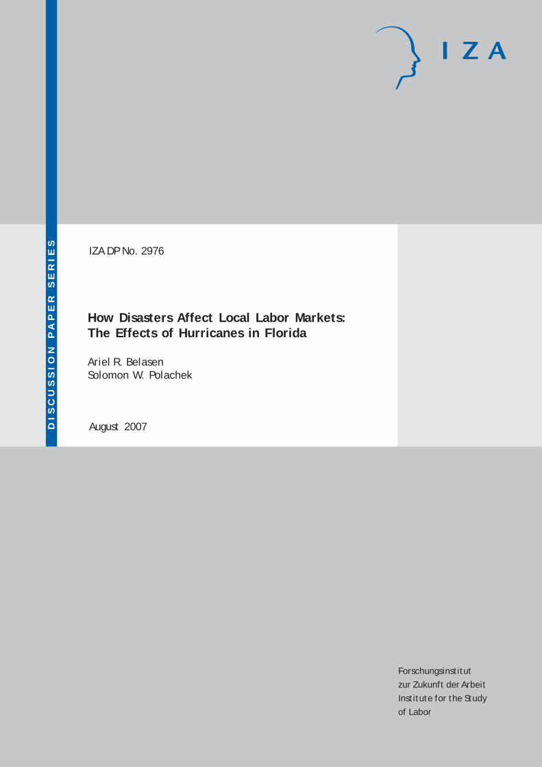
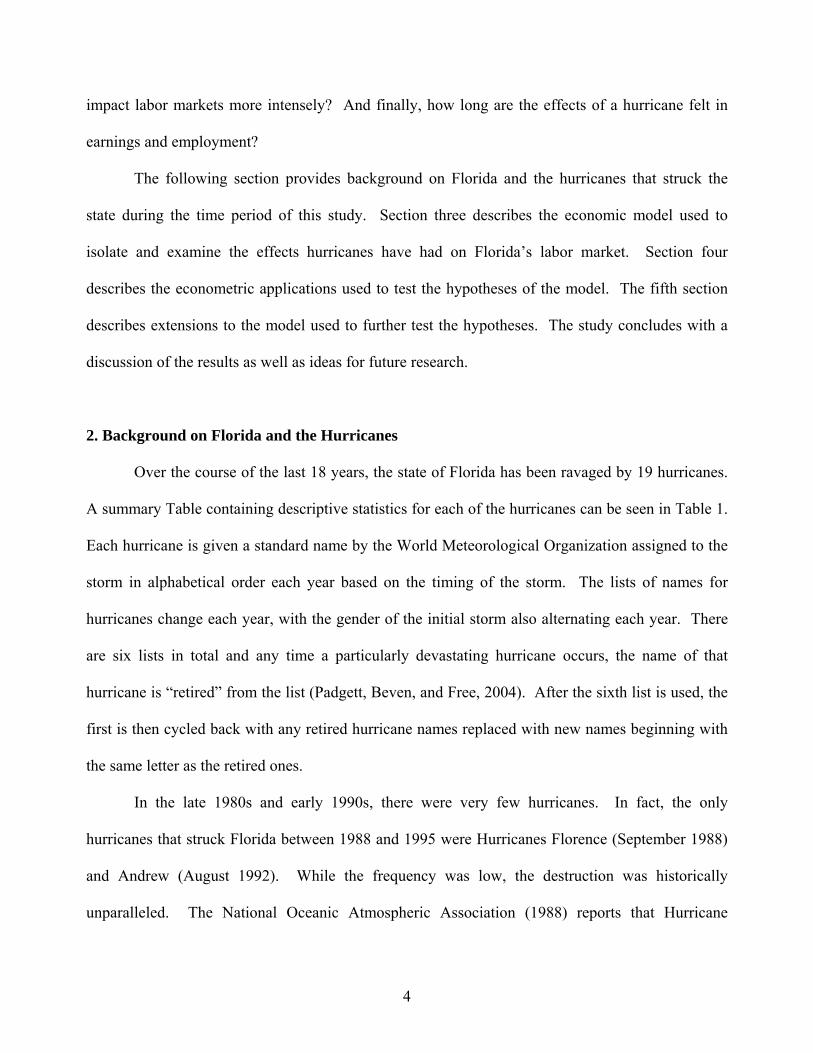
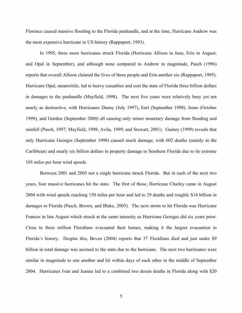
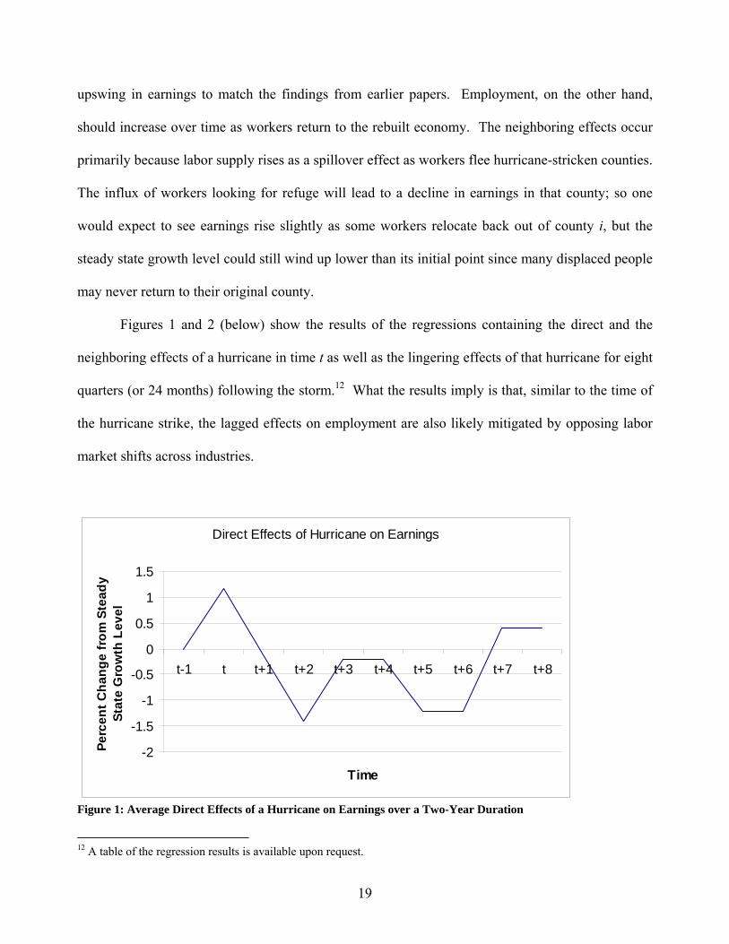
Figures 1 and 2 (below) show the results of the regressions containing the direct and the

neighboring effects of a hurricane in time t as well as the lingering effects of that hurricane for eight

quarters (or 24 months) following the storm.12 What the results imply is that, similar to the time of

the hurricane strike, the lagged effects on employment are also likely mitigated by opposing labor

market shifts across industries.

Direct Effects of Hurricane on Earnings

-2

-1.5

-1

-0.5

0

0.5

1

1.5

t-1 t t+1 t+2 t+3 t+4 t+5 t+6 t+7 t+8

Time

Perc

ent C

hang

e fr

om S

tead

y St

ate

Gro

wth

Lev

el

Figure 1: Average Direct Effects of a Hurricane on Earnings over a Two-Year Duration

12 A table of the regression results is available upon request.

20

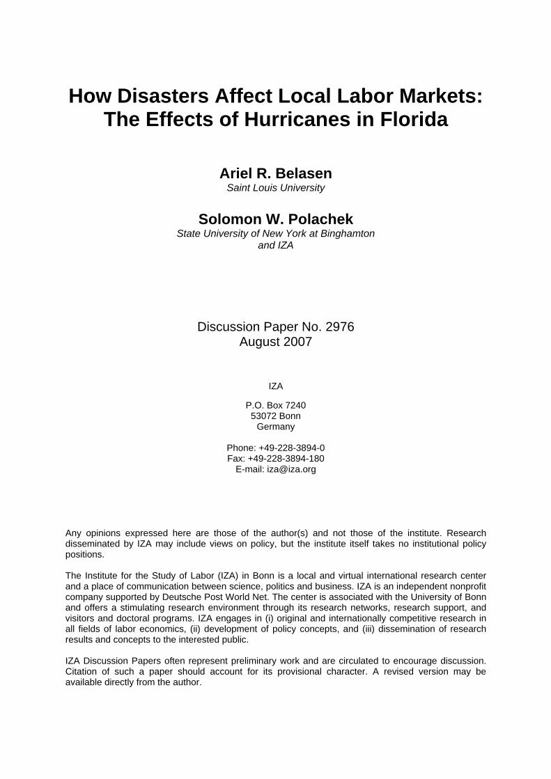
Direct Effects of Hurricane on Employment

-7

-6

-5

-4

-3

-2

-1

0

t-1 t+1 t+3 t+5 t+7 t+9 t+11

t+13

t+15

t+17

t+19

t+21

t+23

Time (monthly)

Perc

ent C

hang

e fr

om S

tead

y St

ate

Gro

wth

Lev

el

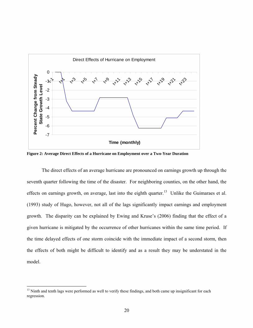
Figure 2: Average Direct Effects of a Hurricane on Employment over a Two-Year Duration

The direct effects of an average hurricane are pronounced on earnings growth up through the

seventh quarter following the time of the disaster. For neighboring counties, on the other hand, the

effects on earnings growth, on average, last into the eighth quarter.13 Unlike the Guimaraes et al.

(1993) study of Hugo, however, not all of the lags significantly impact earnings and employment

growth. The disparity can be explained by Ewing and Kruse’s (2006) finding that the effect of a

given hurricane is mitigated by the occurrence of other hurricanes within the same time period. If

the time delayed effects of one storm coincide with the immediate impact of a second storm, then

the effects of both might be difficult to identify and as a result they may be understated in the

model.

13 Ninth and tenth lags were performed as well to verify these findings, and both came up insignificant for each regression.

21

What can be seen in Figure 1 is that a hurricane will immediately boost growth in earnings

in the counties where it strikes followed by an immediate downturn one quarter later. As time goes

by, earnings growth will continue to follow this pattern before settling in at a new steady state level

roughly 0.40% above the level of growth for an average county. While this in no way indicates that

earnings growth in a hurricane stricken county will permanently remain higher than in a county that

has avoided the hurricane, it does imply that the temporary wage gains may not be as short term as

the ones Guimaraes et al. (1993) reported based on Hurricane Hugo. On the other hand, these

findings are consistent with the existing literature of Ewing et al. (2007) and Ewing and Kruse

(2006) which found that after a hurricane, earnings will jump immediately and then converge back

towards pre-hurricane levels. Additionally, they find that while hurricanes create an economic

disturbance in the short run, oftentimes they can lead to economic gains in the long run, just as we

have found in this paper.

Figure 2 illustrates the cumulative monthly growth rate of employment. We find that the

labor market takes a cobweb form in which employment jumps about a year after the hurricane

(coinciding with a decrease in earnings) and then decreases as earnings increase before settling at a

growth rate 4.32% lower than that of unaffected counties.

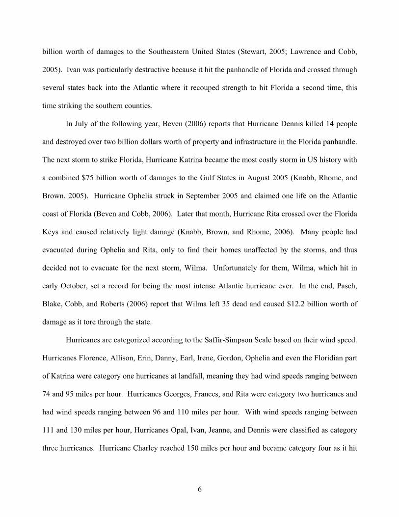
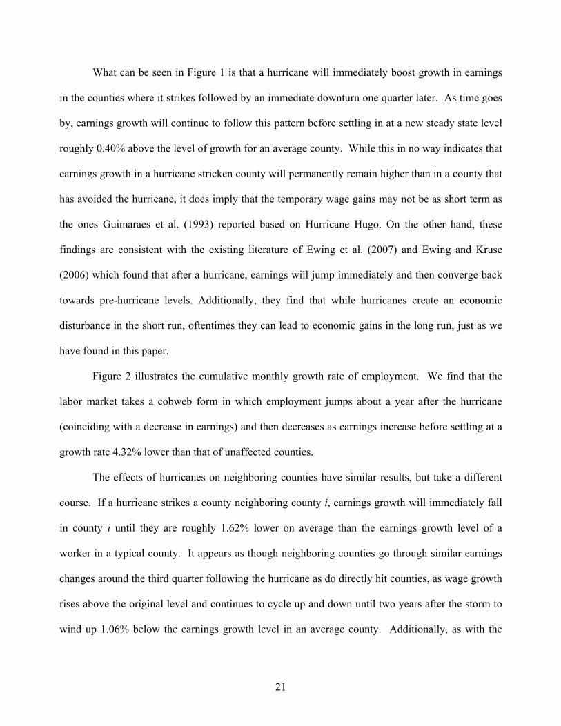
The effects of hurricanes on neighboring counties have similar results, but take a different

course. If a hurricane strikes a county neighboring county i, earnings growth will immediately fall

in county i until they are roughly 1.62% lower on average than the earnings growth level of a

worker in a typical county. It appears as though neighboring counties go through similar earnings

changes around the third quarter following the hurricane as do directly hit counties, as wage growth

rises above the original level and continues to cycle up and down until two years after the storm to

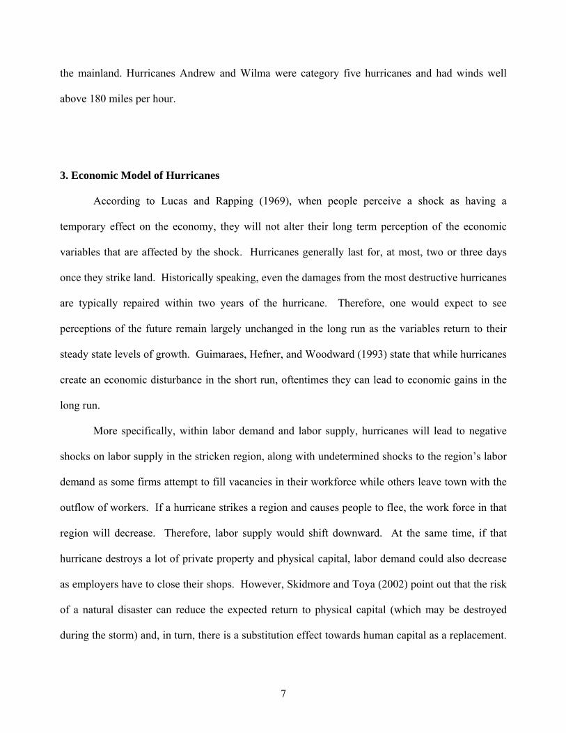
wind up 1.06% below the earnings growth level in an average county. Additionally, as with the

22

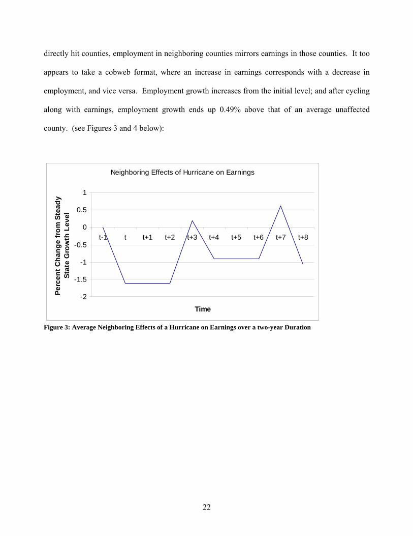
directly hit counties, employment in neighboring counties mirrors earnings in those counties. It too

appears to take a cobweb format, where an increase in earnings corresponds with a decrease in

employment, and vice versa. Employment growth increases from the initial level; and after cycling

along with earnings, employment growth ends up 0.49% above that of an average unaffected

county. (see Figures 3 and 4 below):

Neighboring Effects of Hurricane on Earnings

-2

-1.5

-1

-0.5

0

0.5

1

t-1 t t+1 t+2 t+3 t+4 t+5 t+6 t+7 t+8

Time

Perc

ent C

hang

e fr

om S

tead

y St

ate

Gro

wth

Lev

el

Figure 3: Average Neighboring Effects of a Hurricane on Earnings over a two-year Duration

23

Neighboring Effects of Hurricane on Employment

-1

-0.5

0

0.5

1

1.5

2

2.5

3

t-1 t+1 t+3 t+5 t+7 t+9 t+11

t+13

t+15

t+17

t+19

t+21

t+23

Time (monthly)

Perc

ent C

hang

e fr

om S

tead

y St

ate

Gro

wth

Lev

el

Figure 4: Average Neighboring Effects of Hurricane on Employment over a 2-year Duration

At certain points in time, earnings growth will be higher in hurricane-impacted counties than

in other counties while employment growth will remain relatively unchanged. This is likely a result

of low wage earners being replaced by high wage earners in the specified counties. Card (1990)

and Belasen and Polachek (2007) each have results that are consistent with these findings.14

5.3. Geographic Effects

Thus far, we have studied the effects of hurricanes on three separate groups of counties in

Florida: those that were directly hit by the storm, those neighboring the counties that were directly

hit, and all other counties. Theoretically speaking we expect that the neighboring effect should

diminish with distance, so a town located 100 miles away from a directly hit county should face a

14 Other time-related applications that can be drawn from this particular regression are to see if specific time-related events (such as elections or the September 11 terror attack) had any impact on the hurricane effects. As with the additional specifications for intensity effects, these additional time-related effects were also insignificant. However, it appears that timing within a quarter can alter the impact of a hurricane on the labor market, such that hurricanes that occur early on in the quarter will have less of an effect than other hurricanes. This is likely due to the fact that hurricanes last for a week at most and are typically dealt with soon after (see models 6 and 7 in tables 2 and 3).

24

stronger neighboring effect than a town located 200 miles away since the flooding will be greater as

the proximity to the locus of destruction increases. To verify this expectation, we fit equations (9)

and (10) with a “Second County Away” variable to capture the effects of hurricanes on the counties

which lay two away from the directly hit counties:

24321)lnln( ikt

Nijt

Ditttit HHHSQQ Δ+Δ+Δ+Δ=Δ−Δ αααα (17)

24321)lnln( ikt

Nijt

Ditttit HHHSyy Δ+Δ+Δ+Δ=Δ−Δ δδδδ (18)

The new variable 2iktHΔ takes a value of one for county i when a hurricane strikes county k

if that county k is two counties away from county i. In other words, it is essentially the neighboring

effect of the original neighboring effect. One would, therefore, expect to see the coefficients for the

neighboring effect and the second-county-away effect to take the same sign, but for the second-

county-away coefficient to be smaller in magnitude (or insignificant as the case may be). Model 8

in Tables 2 and 3 report the results of these regressions.

Similar to the neighboring effect, the two-away effect is insignificant for employment. In

fact, the neighboring effect and the second-county-away effect on average earnings are nearly

identical in sign and magnitude. However, the second-county-away effect is less significant, thus

one can argue that it holds up to the theoretical expectations. In addition, we find that the second-

county-away effect is insignificant which also verifies expectations. In sum, we are able to

conclude from this that the neighboring effect of hurricanes found in earnings diminishes with

distance from the path of the storm.

A final extension incorporates geographic location into the model to examine whether

certain areas of Florida are affected more heavily by hurricanes than others. To that end, we

25

differentiate between coastal and landlocked counties, as well as between counties located on the

panhandle or in the rest of the state. Coastal counties experience more flooding than landlocked

counties and generally find themselves facing higher monetary costs for rebuilding. The hurricane

effects, therefore, should be more pronounced for coastal counties. Panhandle counties draw most

of their economic growth from tourism whereas other counties tend to have a better developed

industrial infrastructure. Therefore we expect to see weaker increases in earnings for directly hit

panhandle counties and stronger decreases for neighboring panhandle counties since tourism

revenues are likely to diminish all across the panhandle after a hurricane strikes there. Equations

(9) and (10) are fit with a variable C to distinguish coastal counties from non-coastal counties and a

variable P to distinguish between those counties lying on the panhandle versus all other counties.

Furthermore, a great deal of panhandle counties lie on the coast so there is an interaction between

the two sets of geographic comparisons. To that end, we also separate out those counties that meet

both qualifications by adding in a series of interaction terms for both C and P:

Nijt

Ditttit HHSQQ Δ+Δ+Δ=Δ−Δ 321)lnln( ααα

)*(654 PCPC ααα +++ )*()*( 87 CHCH Nijt

Dit Δ+Δ+ αα

)*()*( 109 PHPH Nijt

Dit Δ+Δ+ αα )**()**( 1211 PCHPCH N

ijtDit Δ+Δ+ αα (19)

Nijt

Ditttit HHSyy Δ+Δ+Δ=Δ−Δ 321)lnln( δδδ

)*(654 PCPC δδδ +++ )*()*( 87 CHCH Nijt

Dit Δ+Δ+ δδ

)*()*( 109 PHPH Nijt

Dit Δ+Δ+ δδ )**()**( 1211 PCHPCH N

ijtDit Δ+Δ+ δδ (20)

26

Models 9, 10, and 11 in Tables 2 and 3 each fit the original model with the coastal and/or

panhandle variables (independently as well as together) and their interactions with the hurricanes.

Coastal counties and panhandle counties tend to have a lower change in employment than the rest of

the state. However, the impact of hurricanes on employment does not appear to be any different

across the different geographic classifications. Both coastal and panhandle counties also exhibit a

greater increase in earnings than the rest of the state. And while there is no discernable difference

between the different types of counties after a direct hit from a hurricane, neighboring effects

change drastically by isolating the geographic characteristics of the county.

Explicitly accounting for the panhandle in Models 10 and 11 appears to somewhat negate

the overall effects of hurricanes on the average neighboring county. Whereas the NijtHΔ coefficient

becomes insignificant, the interaction term between the panhandle and the neighboring hurricane

variables is significantly negative. This implies that neighbors of panhandle counties are the

counties most affected by hurricanes. Relative earnings in these counties fall 3.21 to 5.31% when

their neighbors in the panhandle are hit by a hurricane. Neighbors of coastal states hit by a hurricane

are negligibly affected as earnings fall only by -0.01% (Models 9 and 11). Finally, the magnitude of

employment effects is much greater for both direct and neighboring counties relative to the typical

county if those hurricane-impacted counties lie both along the coast and the Panhandle.

6. Conclusion

As illustrated by hurricanes, exogenous shocks to an economy will lead to opposing shifts in

wages and the size of the labor force across neighboring local labor markets. Therefore exogenous

factors that may not appear to have much of an impact on a macro scale, may yet play a major role

in shaping the differences across local markets.

27

The devastation and frequency of hurricanes in the North Atlantic Ocean is unparalleled

relative to other natural disasters in the United States. The widespread devastation of hurricanes

can wipe out infrastructure, private homes, businesses, and even entire communities. While the

effects can be measured by looking directly at the loss of life and damage to property, there are also

indirect results of a hurricane. One such result is the effect of hurricanes on local labor markets.

This paper developed a GDD model that, through various specifications, isolated two distinct

effects hurricanes have on labor markets. The first involves the specific counties directly struck by

hurricanes. Here the hurricane decreases employment in the stricken counties while at the same

time boosting earnings, thus appearing to negatively impact labor supply, while at the same time

changing the labor demand for certain industrial sectors. And as workers flee the devastation by

heading into neighboring counties, those counties experience a positive labor supply shock moving

the equilibrium downward along what appears to be a perfectly inelastic labor demand curve. The

result is that employment is relatively unchanged, while earnings will have decreased.

We find that as a portion of the labor force flees a hurricane-stricken county, the growth of

earnings per worker remaining in that county of Florida will increase up to 4.35% relative to

workers outside that county. Meanwhile, as workers flow into nearby counties, the growth of

earnings per worker in those regions will decrease by as much as 4.51%. Even two years after the

hurricane, earnings may still remain higher in areas hit by a hurricane than elsewhere.

Particularly in today’s age of increased intensity, duration, and sheer quantity of tropical

storms, policymakers looking to rebuild hurricane damaged economies can point to the wage

benefits for workers who relocate to regions that have been hit by hurricanes. This entails both

short-term and long-term effects on both directly hit and neighboring counties, which we find to

exhibit somewhat of a cobweb quarter-by-quarter. These findings should help policy makers assess

28

such issues as UI eligibility. In addition, it should help policy makers in areas outside of the

Southeast US such as California, Mexico, and Brazil that are now being hit by hurricanes due to

recent weather changes.

Subsequent studies related to Generalized Difference-in-Difference could include the

examination of the impact of unplanned illegal immigration on local economies or the influx of a

new disease. In addition, the exogenous effects of other natural disasters (i.e. earthquakes,

tornados, tsunamis, etc.) could also be captured by this model using the same framework. In

addition, other variables of study could include FEMA funding and other economic specifications

(such as GDP growth, consumer spending, industrial growth, etc.).

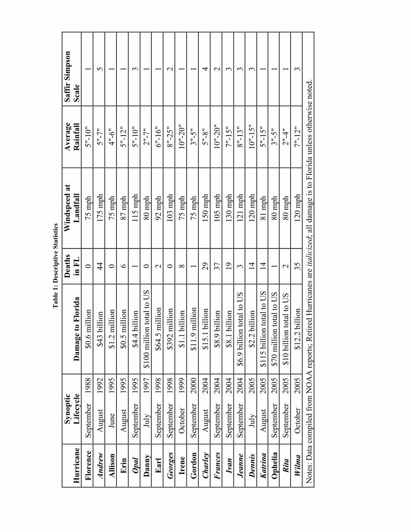
Table 1: Descriptive Statistics

Hurricane

Synoptic

Lifecycle

Damage to Florida

Deaths

in FL

Windspeed at

Landfall

Average

Rainfall

Saffir Simpson

Scale

Florence

Sep

tem

ber

1988

$0.6 m

illion

0

75 m

ph

5"-10"

1

Andrew

August

1992

$43 billion

44

175 m

ph

5"-7"

5

Allison

June

1995

$1.2 m

illion

0

75 m

ph

4"-6"

1

Erin

August

1995

$0.5 m

illion

6

87 m

ph

5"-12"

1

Opal

Sep

tem

ber

1995

$4.4 billion

1

115 m

ph

5"-10"

3

Danny

July

1997

$100 m

illion total to

US

0

80 m

ph

2"-7"

1

Earl

Sep

tem

ber

1998

$64.5 m

illion

2

92 m

ph

6"-16"

1

Georges

Sep

tem

ber

1998

$392 m

illion

0

103 m

ph

8"-25"

2

Irene

October

1999

$1.1 billion

8

75 m

ph

10"-20"

1

Gordon

Sep

tem

ber

2000

$11.9 m

illion

1

75 m

ph

3"-5"

1

Charley

August

2004

$15.1 billion

29

150 m

ph

5"-8"

4

Frances

Sep

tem

ber

2004

$8.9 billion

37

105 m

ph

10"-20"

2

Ivan

Sep

tem

ber

2004

$8.1 billion

19

130 m

ph

7"-15"

3

Jeanne

Sep

tem

ber

2004

$6.9 billion total to

US

3

121 m

ph

8"-13"

3

Dennis

July

2005

$2.2 billion

14

120 m

ph

10"-15"

3

Katrina

August

2005

$115 billion total to

US

14

81 m

ph

5"-15"

1

Ophelia

Sep

tem

ber

2005

$70 m

illion total to

US

1

80 m

ph

3"-5"

1

Rita

Sep

tem

ber

2005

$10 billion total to

US

2

80 m

ph

2"-4"

1

Wilma

October

2005

$12.2 billion

35

120 m

ph

7"-12"

3

Notes: D

ata co

mpiled

fro

m N

OAA rep

orts; R

etired

Hurrican

es are

italicized; all dam

age is to F

lorida unless

oth

erwise noted.

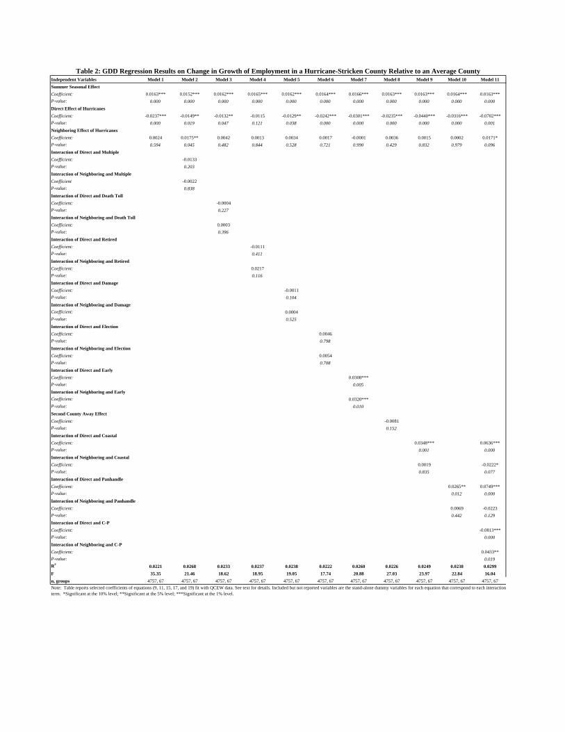
Independent Variables Model 1 Model 2 Model 3 Model 4 Model 5 Model 6 Model 7 Model 8 Model 9 Model 10 Model 11Summer Seasonal EffectCoefficient: 0.0163*** 0.0152*** 0.0162*** 0.0165*** 0.0162*** 0.0164*** 0.0166*** 0.0163*** 0.0163*** 0.0164*** 0.0163***P-value: 0.000 0.000 0.000 0.000 0.000 0.000 0.000 0.000 0.000 0.000 0.000Direct Effect of HurricanesCoefficient: -0.0237*** -0.0149** -0.0132** -0.0115 -0.0129** -0.0242*** -0.0301*** -0.0235*** -0.0440*** -0.0316*** -0.0702***P-value: 0.000 0.019 0.047 0.121 0.038 0.000 0.000 0.000 0.000 0.000 0.001Neighboring Effect of HurricanesCoefficient: 0.0024 0.0175** 0.0042 0.0013 0.0034 0.0017 -0.0001 0.0036 0.0015 0.0002 0.0171*P-value: 0.594 0.045 0.482 0.844 0.528 0.721 0.990 0.429 0.832 0.979 0.096Interaction of Direct and MultipleCoefficient: -0.0133P-value: 0.203Interaction of Neighboring and MultipleCoefficient -0.0022P-value: 0.838Interaction of Direct and Death TollCoefficient: -0.0004P-value: 0.227Interaction of Neighboring and Death TollCoefficient: 0.0003P-value: 0.396Interaction of Direct and RetiredCoefficient: -0.0111P-value: 0.411Interaction of Neighboring and RetiredCoefficient: 0.0217P-value: 0.116Interaction of Direct and DamageCoefficient: -0.0011P-value: 0.104Interaction of Neighboring and DamageCoefficient: 0.0004P-value: 0.525Interaction of Direct and ElectionCoefficient: 0.0046P-value: 0.798Interaction of Neighboring and ElectionCoefficient: 0.0054P-value: 0.708Interaction of Direct and EarlyCoefficient: 0.0308***P-value: 0.005Interaction of Neighboring and EarlyCoefficient: 0.0320***P-value: 0.010Second County Away EffectCoefficient: -0.0081P-value: 0.152Interaction of Direct and CoastalCoefficient: 0.0348*** 0.0636***P-value: 0.001 0.000Interaction of Neighboring and CoastalCoefficient: 0.0019 -0.0222*P-value: 0.835 0.077Interaction of Direct and PanhandleCoefficient: 0.0265** 0.0749***P-value: 0.012 0.000Interaction of Neighboring and PanhandleCoefficient: 0.0069 -0.0223P-value: 0.442 0.129Interaction of Direct and C-PCoefficient: -0.0813***P-value: 0.000Interaction of Neighboring and C-PCoefficient: 0.0433**P-value: 0.019R2 0.0221 0.0268 0.0233 0.0237 0.0238 0.0222 0.0260 0.0226 0.0249 0.0238 0.0299F 35.35 21.46 18.62 18.95 19.05 17.74 20.88 27.03 23.97 22.84 16.04n, groups 4757, 67 4757, 67 4757, 67 4757, 67 4757, 67 4757, 67 4757, 67 4757, 67 4757, 67 4757, 67 4757, 67

Table 2: GDD Regression Results on Change in Growth of Employment in a Hurricane-Stricken County Relative to an Average County

Note: Table reports selected coefficients of equations (9, 11, 15, 17, and 19) fit with QCEW data. See text for details. Included but not reported variables are the stand-alone dummy variables for each equation that correspond to each interaction term. *Significant at the 10% level; **Significant at the 5% level; ***Significant at the 1% level.

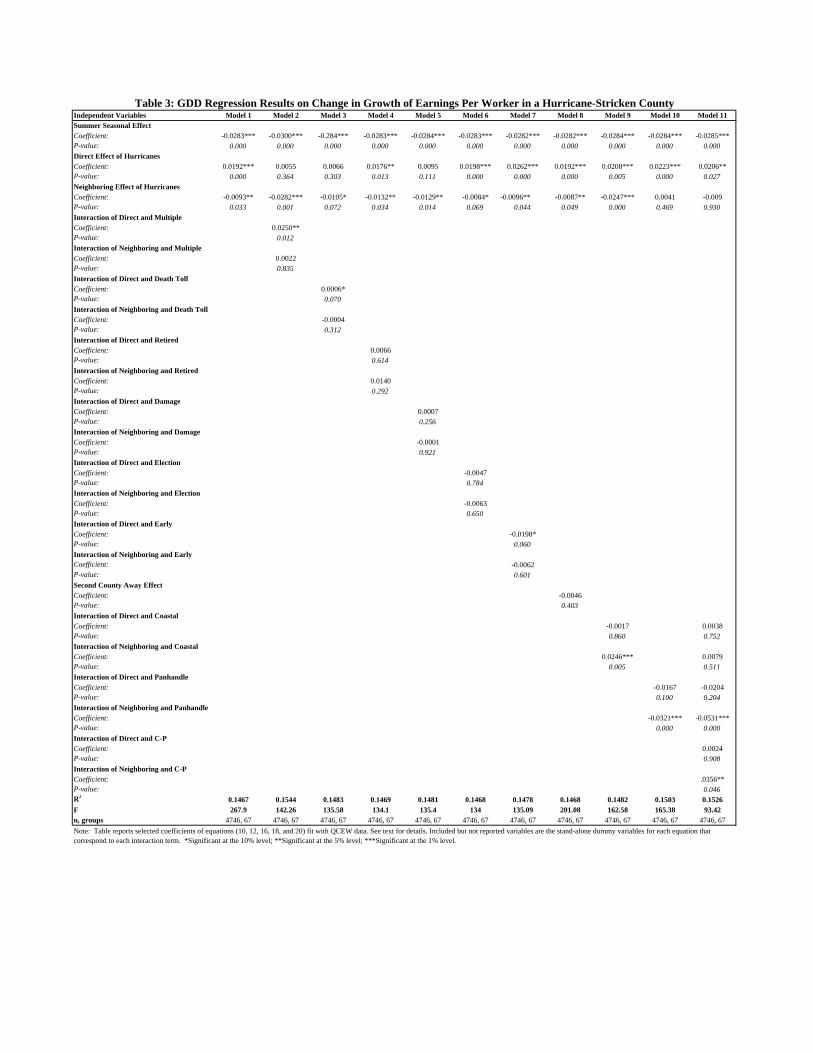
Independent Variables Model 1 Model 2 Model 3 Model 4 Model 5 Model 6 Model 7 Model 8 Model 9 Model 10 Model 11Summer Seasonal EffectCoefficient: -0.0283*** -0.0300*** -0.284*** -0.0283*** -0.0284*** -0.0283*** -0.0282*** -0.0282*** -0.0284*** -0.0284*** -0.0285***P-value: 0.000 0.000 0.000 0.000 0.000 0.000 0.000 0.000 0.000 0.000 0.000Direct Effect of HurricanesCoefficient: 0.0192*** 0.0055 0.0066 0.0176** 0.0095 0.0198*** 0.0262*** 0.0192*** 0.0208*** 0.0223*** 0.0206**P-value: 0.000 0.364 0.303 0.013 0.111 0.000 0.000 0.000 0.005 0.000 0.027Neighboring Effect of HurricanesCoefficient: -0.0093** -0.0282*** -0.0105* -0.0132** -0.0129** -0.0084* -0.0096** -0.0087** -0.0247*** 0.0041 -0.009P-value: 0.033 0.001 0.072 0.034 0.014 0.069 0.044 0.049 0.000 0.469 0.930Interaction of Direct and MultipleCoefficient: 0.0250**P-value: 0.012Interaction of Neighboring and MultipleCoefficient: 0.0022P-value: 0.835Interaction of Direct and Death TollCoefficient: 0.0006*P-value: 0.070Interaction of Neighboring and Death TollCoefficient: -0.0004P-value: 0.312Interaction of Direct and RetiredCoefficient: 0.0066P-value: 0.614Interaction of Neighboring and RetiredCoefficient: 0.0140P-value: 0.292Interaction of Direct and DamageCoefficient: 0.0007P-value: 0.256Interaction of Neighboring and DamageCoefficient: -0.0001P-value: 0.921Interaction of Direct and ElectionCoefficient: -0.0047P-value: 0.784Interaction of Neighboring and ElectionCoefficient: -0.0063P-value: 0.650Interaction of Direct and EarlyCoefficient: -0.0198*P-value: 0.060Interaction of Neighboring and EarlyCoefficient: -0.0062P-value: 0.601Second County Away EffectCoefficient: -0.0046P-value: 0.403Interaction of Direct and CoastalCoefficient: -0.0017 0.0038P-value: 0.860 0.752Interaction of Neighboring and CoastalCoefficient: 0.0246*** 0.0079P-value: 0.005 0.511Interaction of Direct and PanhandleCoefficient: -0.0167 -0.0204P-value: 0.100 0.204Interaction of Neighboring and PanhandleCoefficient: -0.0321*** -0.0531***P-value: 0.000 0.000Interaction of Direct and C-PCoefficient: 0.0024P-value: 0.908Interaction of Neighboring and C-PCoefficient: .0356**P-value: 0.046R2 0.1467 0.1544 0.1483 0.1469 0.1481 0.1468 0.1478 0.1468 0.1482 0.1503 0.1526F 267.9 142.26 135.58 134.1 135.4 134 135.09 201.08 162.58 165.38 93.42n, groups 4746, 67 4746, 67 4746, 67 4746, 67 4746, 67 4746, 67 4746, 67 4746, 67 4746, 67 4746, 67 4746, 67

Table 3: GDD Regression Results on Change in Growth of Earnings Per Worker in a Hurricane-Stricken County

Note: Table reports selected coefficients of equations (10, 12, 16, 18, and 20) fit with QCEW data. See text for details. Included but not reported variables are the stand-alone dummy variables for each equation that correspond to each interaction term. *Significant at the 10% level; **Significant at the 5% level; ***Significant at the 1% level.

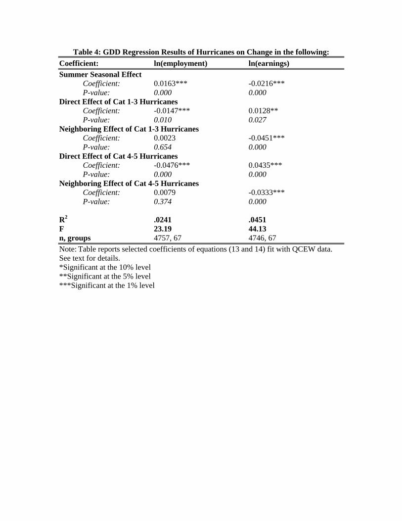
Table 4: GDD Regression Results of Hurricanes on Change in the following: Coefficient: ln(employment) ln(earnings) Summer Seasonal Effect

Coefficient: 0.0163*** -0.0216*** P-value: 0.000 0.000

Direct Effect of Cat 1-3 Hurricanes Coefficient: -0.0147*** 0.0128** P-value: 0.010 0.027

Neighboring Effect of Cat 1-3 Hurricanes Coefficient: 0.0023 -0.0451*** P-value: 0.654 0.000

Direct Effect of Cat 4-5 Hurricanes Coefficient: -0.0476*** 0.0435*** P-value: 0.000 0.000

Neighboring Effect of Cat 4-5 Hurricanes Coefficient: 0.0079 -0.0333*** P-value: 0.374 0.000

R2 .0241 .0451 F 23.19 44.13 n, groups 4757, 67 4746, 67 Note: Table reports selected coefficients of equations (13 and 14) fit with QCEW data. See text for details. *Significant at the 10% level **Significant at the 5% level ***Significant at the 1% level

References:

Abadie, A., Diamond, A., and Hainmueller, J. (2007). “Synthetic Control Methods for Comparative Case Studies: Estimating the Effect of California’s Tobacco Control Problem,” NBER Working Paper 12831.

Angrist J. A. and Krueger A. B. (1999). “Empirical Strategies in Labor

Economics,” in O. C. Ashenfelter and D. A. Card, editors, Handbook of Labor Economics, 3A, Amsterdam: Elsevier, 1277-1366.

Avila, L. (1999). “Preliminary Report: Hurricane Irene,” National Oceanic and

Atmospheric Association, http://www.nhc.noaa.gov/1999irene.html. Belasen, A. and Polachek, S. (2007). “When Oceans Attack: Using a Generalized

Difference-in-Difference Technique to Assess the Impact of Hurricanes on Local Labor Markets,” unpublished working paper, 2007.

Bertrand, M., Duflo, E., & Mullainathan, S. (2002). “How Much Should We Trust

Differences-in-Differences Estimates?,” NBER working paper 8841. Beven, J. (2004). “Tropical Cyclone Report: Hurricane Frances,” National

Oceanic and Atmospheric Association, http://www.nhc.noaa.gov/2004frances.shtml. Beven, J. (2006). “Tropical Cyclone Report: Hurricane Dennis,” National

Oceanic and Atmospheric Association, http://www.nhc.noaa.gov/pdf/TCR-AL042005_Dennis.pdf.

Beven, J. and Cobb, H. D. (2006). “Tropical Cyclone Report: Hurricane Ophelia,”

National Oceanic and Atmospheric Association, http://www.nhc.noaa.gov/pdf/TCR-AL162005_Ophelia.pdf.

Card, D. (1990). “The Impact of the Marial Boatlift on the Miami Labor Market,” Industrial and Labor Relations Review, 43 (2), 245-257. Climate.org (2004). “Brazil Hurricane,”

http://www.climate.org/topics/climate/brazil_hurricane.shtml. Connolly, M. (2007). “Here Comes the Rain Again: Weather and Intertemporal Substitution of

Leisure,” unpublished working paper, 2007. Ewing, B. T., and Kruse, J. B. (2006). “Hurricanes and Unemployment,”

Natural Hazards Review. Ewing, B. T., Kruse, J. B., Thompson, M. A. (2007). “Twister! Employment

Responses to the May 3, 1999, Oklahoma City Tornado,” Journal of Applied Economics (forthcoming).

Google (2006). “Google Earth,” http://earth.google.com. Guimaraes, P., Hefner, F., & Woodward, D. (1993). “Wealth and Income Effects

of Natural Disasters: An Econometric Analysis of Hurricane Hugo,” The Review of Regional Studies, 23, 97-114.

Guiney, J. (1999). “Preliminary Report: Hurricane Georges,” National Oceanic and Atmospheric Association, http://www.nhc.noaa.gov/1998georges.html.

Knabb, R. D., Rhome, J. R., & Brown, D. P. (2005). “Tropical Cyclone Report:

Hurricane Katrina,” National Oceanic and Atmospheric Association, http://www.nhc.noaa.gov/pdf/TCR-AL122005_Katrina.pdf.

Knabb, R. D., Brown, D. P., & Rhome, J. R., (2006). “Tropical Cyclone Report:

Hurricane Rita,” National Oceanic and Atmospheric Association, http://www.nhc.noaa.gov/pdf/TCR-AL182005_Rita.pdf.

Kubik, J. D. and Moran, J. R. (2003). “Can Policy Changes be Treated as Natural Experiments?

Evidence from Cigarette Excise Taxes,” NBER working paper 11068. Lawrence, M. and Cobb, H. D. (2005). “Tropical Cyclone Report: Hurricane

Jeanne,” National Oceanic and Atmospheric Association, http://www.nhc.noaa.gov/2004jeanne.shtml.

Lucas, R. and Rapping, L. (1969). “Price Expectations and the Phillips Curve,”

The American Economic Review, 59 (3), 342-350. Mayfield, M. (1995). “Preliminary Report: Hurricane Opal,” National Oceanic

and Atmospheric Association, http://www.nhc.noaa.gov/1995opal.html. Mayfield, M. (1998). “Preliminary Report: Hurricane Earl,” National Oceanic

and Atmospheric Association, http://www.nhc.noaa.gov/1998earl.html. Miguel, E. (2005). “Poverty and Witch Killing,” Review of Economic Studies, 72 (4), 1153-1172. National Oceanic and Atmospheric Association (1988). “Hurricane Florence,”

http://www.hpc.ncep.noaa.gov/tropical/rain/florence1988.html. National Oceanic and Atmospheric Association (2006). “Hurricanes,”

http://hurricanes.noaa.gov/. National Oceanic and Atmospheric Association (2006). “Retired Hurricane

Names,” http://www.nhc.noaa.gov/retirednames.shtml. Padgett, G., Beven, J., & Free, J. L. (2004). Atlantic Oceanographic and

Meteorological Laboratory, National Oceanic and Atmospheric

Association, http://www.aoml.noaa.gov/hrd/tcfaq/B3.html. Pasch, R. J. (1996). “Preliminary Report: Hurricane Allison,” National Oceanic

and Atmospheric Association, http://www.nhc.noaa.gov/1995allison.html. Pasch, R. J. (1997). “Preliminary Report: Hurricane Danny,” National Oceanic

and Atmospheric Association, http://www.nhc.noaa.gov/1997danny.html. Pasch, R. J., Blake, E. S., Cobb, H.D., & Roberts, D. P. (2006). “Tropical Cyclone

Report: Hurricane Wilma,” National Oceanic and Atmospheric Association, http://www.nhc.noaa.gov/pdf/TCR-AL252005_Wilma.pdf.

Pasch, R. J., Brown, D. P., & Blake, E. S. (2005). “Tropical Cyclone Report:

Hurricane Charley,” National Oceanic and Atmospheric Association, http://www.nhc.noaa.gov/2004charley.shtml.

Pew Center on Global Climate Change (2006). “Global Warming and

Hurricanes,” http://www.pewclimate.org/hurricanes.cfm/. Rappaport, E. (1993). “Preliminary Report: Hurricane Andrew,” National Oceanic

and Atmospheric Association, http://www.nhc.noaa.gov/1992andrew.html. Rappaport, E. (1995). “Preliminary Report: Hurricane Erin,” National Oceanic

and Atmospheric Association, http://www.nhc.noaa.gov/1995erin.html. Skidmore, M. and Toya, H. (2002). “Do Natural Disasters Promote Long-Run

Growth?” Economic Inquiry, 40, 664-687. Stewart, S. (2001). “Preliminary Report: Hurricane Gordon,” National Oceanic

and Atmospheric Association, http://www.nhc.noaa.gov/2000gordon.html. Stewart, S. (2005). “Tropical Cyclone Report: Hurricane Ivan,” National Oceanic

and Atmospheric Association, http://www.nhc.noaa.gov/2004ivan.shtml. US Geological Survey (2006). “SOFIA: South Florida Information Access,”

http://sofia.usgs.gov.

Waldman, M., Nicholson, S., Adilov, N. (2006). “Does Television Cause Autism?,” NBER working paper 12632.