How to Perform Optimization in HEC-HMS

1. To optimize, you should have an observed flow in at least one of the elements in your

model. In this case you will have an observed flow at the outlet of your basin. You should

enter this flow data using time series manager.

2. Select Components | Time Series data manager. Then choose Discharge Gages as the

data type click New and Enter the name. Then click on Create and close the time series

manager.

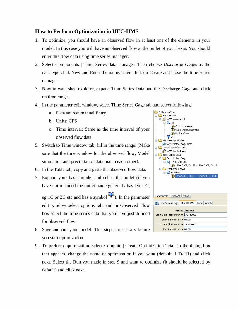
3. Now in watershed explorer, expand Time Series Data and the Discharge Gage and click

on time range.

4. In the parameter edit window, select Time Series Gage tab and select following;

a. Data source: manual Entry

b. Units: CFS

c. Time interval: Same as the time interval of your

observed flow data

5. Switch to Time window tab, fill in the time range. (Make

sure that the time window for the observed flow, Model

simulation and precipitation data match each other).

6. In the Table tab, copy and paste the observed flow data.

7. Expand your basin model and select the outlet (if you

have not renamed the outlet name generally has letter C,

eg 1C or 2C etc and has a symbol ). In the parameter

edit window select options tab, and in Observed Flow

box select the time series data that you have just defined

for observed flow.

8. Save and run your model. This step is necessary before

you start optimization.

9. To perform optimization, select Compute | Create Optimization Trial. In the dialog box

that appears, change the name of optimization if you want (default if Trail1) and click

next. Select the Run you made in step 9 and want to optimize (it should be selected by

default) and click next.

10. Click Finish You have created optimization trial but you need to define what

optimization function you want to use and which parameters you want to optimize. In the

watershed explorer, switch to Compute tab and expand Optimization Trials and Trial1.

Click on Optimization function and select the optimization method you want to use and

make sure that the Time Range is correct in properties edit window.

11. Now to define the parameters you want to optimize, right click on Trial1 under

optimization trials in the watershed explorer. Select Add parameter. This will add

Parameter 1 under objective function. You might want to add as many parameters as you

want to optimize (For eg if you want to optimize 4 parameters in your G and A model,

then you need to add 4 parameters).

12. Click on Parameter 1 and in parameter edit window, select the name of element (name of

basin in this case) and name of parameter. This will display the maximum and minimum

values of the parameter. You can edit that range. Perform the same process to define all

the parameters for optimization.

13. Save your project, right click Trial1 and select Compute. It might take a while to finish.

14. After completion, you can see optimized hydrographs (compared with the observed flow)

by switching to Results tab.

Here you should be able to distinguish between Run1 and Trial1. Run1 is for the general

hydrologic model run that you have been doing so far where as Trial1 is for the optimization

trial. So, to view the results of optimization, you should select Trial1.

15. It might not be a good idea to have all the parameters get optimized at the same time.

After few trials by changing the initial estimate of the parameters you will figure out how

each parameter affects the hydrograph. You can then choose the parameter/s to optimize

at a time.

16. Let us say you have 3 parameters (CN, time of concentration, lag time) and you do not

want CN to get optimized while you calibrate the other two. To do this, select the

parameter which you want to lock from getting optimized in the Compute tab. In the

parameter edit window, select Yes under Locked option. Then run the optimization trial

which will optimize the model while keeping the locked parameter unchanged.

17. To view the optimized parameters, select Results | Optimized Parameters which will open

Optimized Parameter Result dialog with the list of all the parameters you have optimized.