How to Solve Mathematical

Problems

Wayne A. Wickelgren

How to Solve Problems ELEMENTS OF A THEORY OF PROBLEMS

AND PROBLEM SOLVING

Wayne A. Wickelgren UNIVERSITY OF OREGON

rn w. H. FREEMAN AND COMPANY

San Francisco

The Dover reprint added "Mathematical" to the title.

Library of Congress Cataloging in Publication Data

Wic kelgren, Wayne A 1938-How to solve problems.

B i bl iography: p. 1. Mathematics- Problems, exercises, etc.

2. Problem solv i ng. I. Title. QA43.w52 511 73-15787 ISBN 0-7167-0846-9 ISBN 0-7167-0845-0 (pbk.)

Copyright @1974 by W. H. Freeman and Company

No part of this book may be reproduced by any mechan ical, ph otograph ic, or electron i c process, or in the form of a phonograph ic record i ng, nor may it be sto red in a retr ieval system, transm itted, or otherwise copied for publi c or pr ivate use without written permisS ion of the publ isher.

Pr inted in the Un ited States of America

1 2 3 4 5 6 7 8 9

For as long as I can remember, I have been more interested in reflecting on what I was doing or thinking and in thinking about ways to impro ve my methods than I have been in the particular things I was doing or thinking about. This emphasis on self-analysis and improvement reflects the influence of my m o ther and fa ther, Alma and Herman Wickelgren, to whom this book is dedicated and whose values and practical principles have contributed so much to my life.

Preface ix

1 Introduction

2 Problem Theory 7 3 Inference 21

Contents

4 Classification of Action Sequences 46 5 State Evaluation and Hill Climbing 67 6 Subgoals 91 7 Contradiction 109 8 Working Backward 137 9 Relations Between Problems 152

10 Topics in Mathematical Representation 184 11 Problems from Mathematics, Science, and

Engineering 209 References 257 Index 259

Preface

I n the mathematics and science courses I took in college, I was enor­mously irritated by the hundreds of hours that I wasted staring at problems without any good idea about what approach to try next in attempting to solve them. I thought at the time that there was no edu­cational value in those "blank" minutes , and I see no value in them today . The general problem-solving methods described in this book virtually guarantee that you wi l l never again have a b lank mind in such circumstances. They should also help you solve many more problems and solve them faster. But whether or not you solve any particular problem, you will always have lots of ideas about ways to attack the problem. Also, the use of general problem-solving methods often indi­cates the properties of the principles you need to know from the sub­ject matter that the problem is attempt ing to teach and test . Thus , whether you succeed of fai l in solving any particular prob lem, the effort wi l l be interesting and educational .

The theoretical and practical analyses of problems and problem solving presented here were heavi ly influenced by advances made over the last 20 years in the fields of artificial intel l igence and com­puter simulation of thought. My greatest intellectual debts are to Allen Newel l , Herbert Simon , and George Polya. Newell and Simon' s

x Preface

analyses of problems and problem solving constituted my starting point for working in this area, and many of the best ideas in the book are ideas they have already presented in one form or another. Many other good ideas were taken more or less directly from Polya, whose books on mathematical problem solving are a rich sou rce of methods and a stimulus for thought.

My efforts to understand and organize problem-solving methods began in 1 959 when, as an undergraduate at H arvard , I first became aware of the pioneering work of Allen Newel l , Cliff Shaw, and Herb Simon on the computer simulation of thinking. During graduate school at the U niversity of California, Berkeley , I regarded problem solving as my major research area. I do not think that my experimental studies of human problem solving ever amounted to much. However, I thought at the time (and think today) that my theoretical (mathematical) under­standing of prob lems and prob lem solving was immeasurab ly in ­creased and that th is greatly enhanced my ability to solve al l kinds of mathematical problems. Shortly after coming to M IT as a new facuIty member in the Psychology Department, I decided that one contribution I could make to the undergraduates there was to teach them this newly acquired skil l of mathematical problem solving. The students enjoyed the course and , more important, reported back to me in later years that they thought that their problem-solving abi l ity in mathematics , science , and engineering courses had been greatly increased by learning these general problem-solving methods . En­rol lment in the course went from 20 to 80 in three years , when I stopped giving it because my primary research interest had shifted to human memory . Some years later, after moving to the U niversity of Oregon, I decided that I now had the time to write a book containing al l the ideas that I had acquired from others and generated myself concerning problems and problem solving.

The purpose of the book is to improve your ability to solve all kinds of mathematical problems whether in mathematics , science , en­gineering, business, or purely recreational mathematical problems (puzzles , games , and so on). This book is primari ly intended for col­lege students who are currently taking elementary mathematics , science, or engineering courses . However, I hope that students with less mathematical background can read the book and master the methods without an undue degree of additional effort and also that more advanced readers wil l profit from it without being bored. I believe that almost everyone who solves mathematical problems can profit substantial ly from learning the general problem-solving methods

Preface xi

described here , and I have tried to write in a way that wi l l communi­cate effectively to al l such people. The approach is to define each general problem-solving method and i l l ustrate i ts application to s imple recreational mathematics problems that require no more mathematical background than that possessed by someone with a year of high school algebra and a year of plane geometry . An elementary knowledge of "new mathematics" (sets, re lations , functions, probabil ity, and so on) would be helpfu l , and some of thi s i s briefly taught in Chapter 1 0 .

The solu tions to example problems are presented gradual ly , usual ly in the form of h in t s to give the reader more and more chances to go back and solve the problem. This technique is founded on the bel ief that you wi l l remember best what you discover for yourse lf. The book aims to guide you to di scovering how to apply general prob lem-solving methods to a rich variety of problems . I believe that if you read this book and try to apply the methods to around 50 or 100 of your own problems, you wi l l improve substantial ly in problem-solving abi l i ty , with consequent benefits in job performance , school grades , and " in­te l l igence" test scores ( i nc luding SAT col lege entrance exams, and The Graduate Record Exam).

Final ly , I would l ike to make a negat ive acknowledgment . This book was written in spite of my four-year-old son, Abraham, and my s ix­year-old daughter, I ngrid , who are such del ightful people that I cannot resist spending vast amounts of t ime with them.

October 1973 Wayne A . Wicke/gren

How to Solve Problems

1

Introduction

The purpose of this book is to help you improve your ability to solve mathematical , scientific , and engineering problems. With this in mind, I will describe certain elementary concepts and principles of the theory of problems and problem solving, something we have learned a great deal about since the 1 950s, when the advent of computers made pos­sible research on artificial intel l igence and computer simulation of human problem solving. I have tried to organize the discussion of these ideas in a simple, logical way that wi l l help you understand , remember, and apply them.

You should be warned, however, that the theory of problem solving is far from being precise enough at present to provide simple cookbook instructions for solving most problems. Partly for this reason and partly for reasons of intrinsic merit, teaching by example i s the primary ap­proach used in this book. First, a problem-solv ing method wil l be discu ssed theoretical ly, then it wil l be applied to a variety of problems, so that you may see how to use the method in actual practice.

To master these methods , it i s essential to work through the examples of their appl ication to a variety of problems. Thus , much of the book is devoted to analyzing problems that exempl ify the use of different methods . You should pay careful attention to these problems and

2 Chapter 1

should not be discouraged if you do not perfectly understand the the­oretical d iscussions. The theory of problem solving will undoubtably help those students with sufficient mathematical background to under­stand it , but students who lack such a background can compensate by spending greater time on the examples.

SCOPE OF THE BOOK

This book i s primari ly a practical guide to how to solve a certain class of problems, specifically, what I call formal problems or just "prob­lems" (with the adjective formal being understood in later contexts). Formal problems include all mathematical problems of either the "to find" or the "to prove" character but do not include problems of de­fining "mathematical ly interesting" axiom systems. A student taking mathematics courses will hard ly be aware of the practical significance of this exclusion, since defining interesting axiom systems is a prob­lem not typical ly encountered except in certain areas of basic research in mathematics . Similarly, the problem of constructing a new mathe­matical theory in any field of science is not a formal problem, as I use the term, and I wil l not discuss it in thi s book. However, any other mathematical problem that comes up in any field of science, engineer­ing, or mathematics is a formal problem in the sense of this book.

Problems such as what you should eat for breakfast, whether you should marry x or y, whether you should drop out of school , or how can you get yourself to spend more time studying are not formal prob­lems. These problems are virtual ly impossible at the present time to turn into formal problems because we have no good ways of restrict­ing our thinking to a specified set of given information and operations (courses of action we might take) , nor do we often even know how to specify precisely what our goals are in solving these problems. Under­standing formal problems can undoubtedly make some contributions to your thinking in regard to these poorly specified personal problems, but the scope of the present book does not include such problems. Even if it did, it would be extremely difficult to specify any precise methods for solving them.

H owever, formal problems include a large class of practical problems that people might encounter in the real world, although they usually encounter them as games or puzzles presented by friends or appearing in magazines. A practical problem such as how to build a bridge across a river i s a formal problem if, in solving the problem, one is l imited to some specified set of materials (givens) , operations , and , of course, the goal of getting the bridge bui lt .

Introduction 3

I n actuality, you might l imit yourself in this way for a whi le and , if no solution emerged, decide to consider the use of some additional materials, if possible. Expanding the set of given materials (by means other than the use of acceptable operations) is not a part of formal prob­lem solving, but often the situation presents certain givens in sufficiently disgu ised or implicit form that recognition of all the givens i s an im­portant part of skil l in formal problem solving. That ski l l wil l be discussed later.

Practical problems or puzzles of the type we wil l consider differ from problems in mathematics , science, or engineering in that to pose them requ ires less background information and training. Thus , puzzle problems are especial ly suitable as examples of problem-solving methods in this book, because they communicate the workings of the methods most easi ly to the widest range of readers. For this reason, puzzle problems wi l l constitute a large proportion of the examples used in this book - at least prior to the last chapter.

I n principle, it might seem that most important problem-solving methods would be unique to each special ized area of mathematics, science, or engineering, but this is probably not the case. There are many extremely general problem-solving methods , though, to be sure, there are also special methods that can be of use in only a l imited range of fields .

I t may be quite difficult to learn the special methods and knowledge required in a particular field, but at least such methods and knowl­edge are the specific object of instruction in courses . By contrast, general problem-solving methods are rarely, if ever, taught, though they are quite helpful in solving problems in every field of mathematics , science, and engineering.

GENERAL VERSUS SPECIAL METHODS

The relation between specific knowledge and methods , on the one hand, and general problem-solving methods , on the other hand , ap­pears to be as fol lows. When you understand the relevant material and specific methods quite wel l and already have considerable ex­perience in applying this knowledge to s imilar problems, then in solv­ing a new problem you use the same specific methods you used before . Considering the methods used in similar problems is a general problem­solving technique. However, in cases where it is obvious that a par­ticular problem is a member of a class of problems you have solved before , you do not need to make explicit, conscious use of the method : simply go ahead and solve the problem, using methods_ that you have

4 Chapter 1

learned to apply to this class. Once you have this level of under­standing of the relevant material , general problem-solving methods are of l i tt le value in solving the vast majority of homework and examina­tion problems for mathematics, science , and engineering courses.

When problems are more complicated , in the sense of involv ing more component steps , and are not high ly simi lar to previou sly solved problems, the use of general problem-solving methods can be a sub­stantial aid in solution. However, such complex problems wi l l be en­countered only rarely by the beginning mathematics , science, and engineering students taking courses in high school and college. More important to the immediate needs of such students is the role of gen­eral problem-solving methods in simple homework and examination problems where one does not completely understand the re levant material and does not have considerable experience in solving the relevant class of problems. In such cases , general problem-solving methods serve to guide the student to recognize what relevant back­ground information needs to be understood . For example, when one understands the general problem-solving method of setting subgoal s , one can often set particular subgoal s that directly indicate what types of specific information are being tested (and thereby taught) by a particular problem. One then knows what sections of the textbook to reread in order to understand the relevant material .

I f, however, the book is not avai lable, as in many examination situations , general problem-solving methods provide one with powerful general methods for retrieving from memory the relevant background information. For example, the use of general problem-solv ing methods can indicate for which quantities one needs a formula and can provide a basis for choosing among d ifferent al ternative formulas. Frequently, a student may know all the definitions, formulas, and so on, but not have strong associations to this knowledge from the cues present in each type of problem to which this knowledge is relevant.

With experience in solving a variety of problems to which the knowledge is relevant, one will develop strong direct associations between the cues in such problems and this relevant knowledge. How­ever, in the early stages of learning the material , a student wi l l lack such direct associations and will need to u se general problem-solving methods to indicate where in one 's memory to retrieve relevant in­formation or where in the book to look it up. Assuming this idea is true (and this book aims to convince you it is) , mastering general problem-solving methods is important to you both so you can use prob­lems as a learning device and so you can achieve the maximum range of applicabil ity of the knowledge you have stored in mind - on an examination, on a job, or whatever.

Introduction 5

The goal of this book is to teach as many of these general problem­solving methods as I know about, so that if you spend the time to master these methods you can more effectivel y learn the subject matter of your courses . A l so, since the abi l i ty to u se the information given in most mathematics , science, and engineering courses is often pri­mari ly the abil ity to solve problems in these fields, the book aims to increase this abil ity to use knowledge .

RELATION TO ARTIFICIAL INTELLIGENCE

It shou ld be emphasized that this text is primari l y a practical how-to­do-it book in a field where the level of precise (mathematical) formula­tion is far below what I am sure it wi l l be in the future , perhaps even the near future . Artificial inte l l igence and computer simulation of human problem solv ing are cu rrently very active fields of research, and results from some of this work have heavi ly influenced this book. However, theoretical formulations of problem solving superior to those we currently have wi l l eventual l y make the present formulation outdated . Nevertheless, the methods described in the present book , however imperfectly, can be of substantial benefit to any student who masters them. When someone has a beautifu l mathematical theory of problems and problem solv ing sometime in the future , then c learer and more effective how-to-do-it books can be written . Meanwhile, it is my hope that th is book wil l help many people to solve problems better than they did before .

APPLYING METHODS T O PROBLEMS

As discussed previously, to master the problem-solving methods de­scribed in this book, it is necessary to study the example problems il­lu strating their u se . The problems and solutions analyzed in Chapters 3 to 1 0 i l lu strate the use of the methods discussed in the particular chapter. Chapter 1 1 considers a variety of homework and examination problems for mathematics , science, and engineering courses . Of course, you probably have lots of your own problems to solve in school or work, and you should begin u sing the methods on these problems immediately. Merely reading this book provides only the beginning concepts necessary to mastering general problem-solving methods . Practice in us ing the methods is essential to achieving a h igh level of ski l l .

6 Chapter 1

Everyone who solves problems uses many or al l of the methods described in this book, but if you are not an extremely good problem solver, you may be using the methods less effective ly or more hap­hazard ly than you could be by more expl icit training in the methods. At first , the appl ication of such expl icitly taught problem-solv ing methods involves a rather slow, conscious analysis of each problem.

There is no particular reason to engage in th is carefu l , conscious analys is of a problem when you can immediate ly get some good ideas on how to solve it. Just go ahead and sol ve the problem "natural ly ." However, after you solve i t or, even better, while you are solving it , anal yze what you are doing. I t wil l greatly deepen your understanding of problem-solving methods , and you might discover new methods or a new appl ication of an old method.

As you get extensive practice in using these problem-solv ing methods you should become so ski l led in their use that the process becomes less conscious and more automatic or natural . This is the way of al l ski l l learning, whether driving a car, playing tenni s , or solving mathematical problems.

2

Problem Theory

FOUR SAMPLE PROBLEMS

To il lustrate the concepts involved in the theory of problems described in this chapter, we will begin with four sample problems.

Instant Insanity

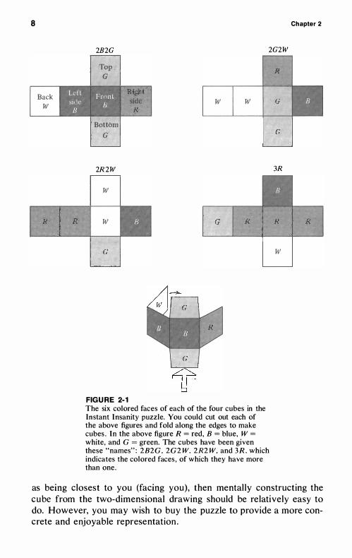
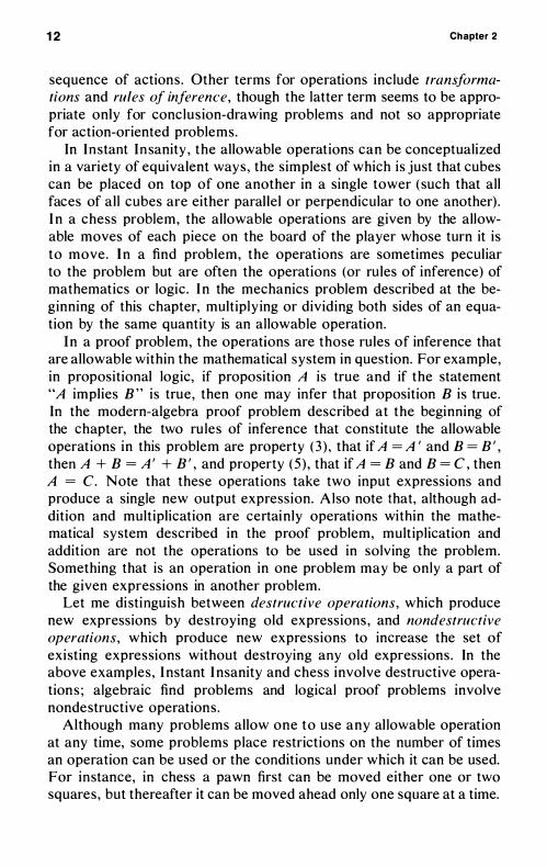
J nstant J nsanity i s the name of a popular puzzle consisting of four smal l cubes . Each face of every cube has one of four colors : red (R) , blue (B ) , green (G ) , or white ( W ) . Each cube has a t least one of its six faces with each of the four different colors, but the remaining two faces necessari ly must repeat one or two of the colors already used.

The exact configurations of colors on the faces of the cubes are shown in Fig. 2- 1 . The faces of the cubes in the figure have been cut along the edges and flattened out for easy presentation on the two­dimensional page . (To reconstruct the cube in three-dimensions, one would simply cut out the outlined figure , turn the top flap over on the top and the bottom over on the bottom, and wrap the left side and back around to join up with the right side at the rear of the cube . ) For con­venience, the faces of one cube in the figure have been labeled front, top, bottom, back, left side, right side. I f you think of the front cube

8

Back W

R:

2B2G 2G2W

I �p I Bottom

G

2R2W

W

W

G

�R�igh'""!"'""t'" side

R

FIGURE 2-1

W W

G R

The six colored faces of each of the four cubes in the Instant Insanity puzzle. You could cut out each of the above figures and fold along the edges to make cubes. In the above figure R = red, B = blue, W =

white, and G = green. The cubes have been given these "names": 2B2G. 2G2W. 2R2W. and 3R. which indicates the colored faces, of which they have more than one.

R

G

G

3R

R

W

Chapter 2

R

as being closest to you (facing you), then mental ly constructing the cube from the two-dimensional drawing should be relatively easy to do. However, you may wish to buy the puzzle to provide a more con­crete and enjoyable representation .

Problem Theory 9

The goal of the puzzle is to arrange the cubes one on top of the other in such a way that they form a stack four cubes high , with each of the four sides having exactly one red cube, one blue cube, one green cube, and one white cube.

Chess Problem

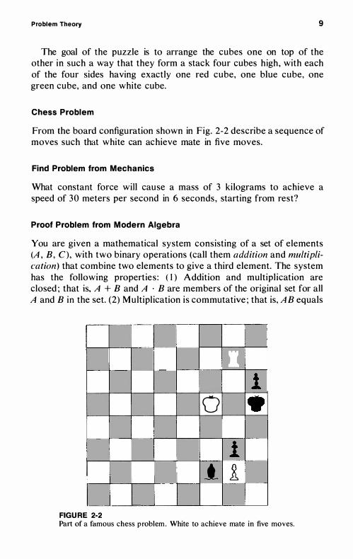
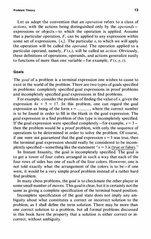
From the board configuration shown in Fig. 2-2 describe a sequence of moves such that white can achieve mate in five moves.

Find Problem from Mechanics

What constant force will cause a mass of 3 kilograms to achieve a speed of 30 meters per second in 6 seconds , starting from rest?

Proof Problem from Modern Algebra

You are given a mathematical system consisting of a set of elements (A , B, C), with two binary operations (call them addition and multipli­cation) that combine two elements to give a third element. The system has the following properties : ( I ) Addition and multiplication are closed ; that is, A + B and A . B are members of the original set for all A and B in the set. (2) Multipl ication is commutative ; that is, A B equals

o_ f

0 '"

i .t it

FIGURE 2-2 Part of a famous chess problem . White to achieve mate in five moves.

10 Chapter 2

BA for all A and B in the set. ( 3 ) Equals added to equal s are equal ; that i s , if A = A I and B = B I, then A + B = A I + B I, for all A , B , A I, B I in the set. (4) The left distributive law appl ie s ; that is , C(A + B) = CA + CB, for all A , B , C in the set. (5 ) The transitive law also applies ; that is , if A = B and B = C, then A = C. From these given assumptions, you are to prove the right distributive law - that i s , that (A + B )C = A C + BC, for all A , B , C in the set.

WHAT IS A PROBLEM?

All the formal problems of concern to us can be considered to be composed of three types of information : information concerning givens (given expressions), information concerning operations that transform one or more expressions into one or more new expressions, and in­formation concerning goals (goal expressions). There may be inter­mediate subgoal expressions mentioned explicitl y in the problem, or the problem solver may define these subgoal expressions for himself; but we wil l assume that there is only one terminal goal per problem. Any problem stated with two or more independent terminal goals could always be viewed as two or more problems with the same givens and operations and different goals .

For convenience and accuracy, I tend to take the more formal view that a problem involves expressions of information rather than actual physical objects. Even in a practical problem stated in terms of physical objects, it is always possible to consider objects or sets of properties of objects as represented by expressions. I ndeed, we must have representations in our heads of objects, properties of objects, and op­erations when we solve practical problems, since we certainly do not have the real objects there . Thus, definitions of problems, solutions, and methods need not make any distinction between practical (con­crete) and symbolic (abstract, mathematical ) . However, when dealing with a practical problem, there is no need to tal k of representations or expressions, if the problem is more easily solved without using this more abstract language.

Givens

G ivens refer to the set of expressions that we accept as being present in the world of the problem at the onset of work on the problem. I n­deed , the givens and the operations together constitute the entire world of the problem at the beginning of work on it. This definition of the givens encompasses expressions representing objects, things, pieces

Problem Theory 11

of material , and so on, as well as expressions representing assump­tions, definitions , axioms, postulates , facts, and the l ike.

In some kinds of puzzles the givens consist of the material s . For example , the givens in I nstant Insanity are four cubes , with each side of each cube having one of four colors (red, blue, green , or white) , as shown in Fig. 2- 1 .

I n the chess problem, the givens are the pieces of each player and their positions on the board plus the information concerning whose move it is. In the particular chess problem shown in Fig. 2-2, the givens are that white has a king, a rook, and a pawn at the positions indicated ; that black has a king, a bishop, and two pawns at the posi­tions indicated ; and that it is white ' s move. The implicitly specified given information consists of al l the rules of chess, including such in­formation as that a rook can move any number of squares along a row or column until blocked by another piece, that a king can move one square in any direction (horizontal ly, vertical ly, or diagonal ly) , that checkmate consists of putting the opponent's king into a position where it would be captured on the next move if it was not moved out of the square it was in and such that all squares that the king could move to would al so result in capture .

I n the find problem, the givens are the information explicitl y stated in the problem plus whatever other mathematical or scientific knowl­edge is to be implicitly assumed as part of the givens. In the physics problem described above, the explicit ly described given information includes the following: the mass of the given object is 3 kilograms, its initial speed is zero, its final speed after 6 seconds of applying a force is 30 meters per second, and the force and mass are constant. I m­plicitly specified information include Newton's second law that force equals mass times acceleration , and the rules of algebra and possibly calculus (depending upon how one solves the problem).

In a mathematical proof problem, the givens are all the axioms that one is allowed to assume. The givens in the particular proof problem described above are three of the five assumptions : ( 1 ) that the system is closed, (2) that multiplication i s commutative, and (4) that the left distributive law holds . Assumptions ( 3 ) , that equals added to equals are equal , and (5 ) , that the transitive law holds (that is, if A = B and B = C, then A = C) are real l y rules of inference rather than givens. Rules of inference are operations, discussed below.

Operations

Operations refer to the actions you are allowed to perform on the givens or on expressions derived from the givens by some previous

1 2 Chapter 2

sequence of actions . Other terms for operations include transforma­tions and rules of inference, though the latter term seems to be appro­priate only for conclusion-drawing problems and not so appropriate for action-oriented problems.

In I n stant I n sanity , the allowable operations can be conceptualized in a variety of equivalent ways , the simplest of which is just that cubes can be placed on top of one another in a single tower (such that all faces of al l cubes are either paral lel or perpendicular to one another) . I n a chess problem, the allowable operations are given by the allow­able moves of each piece on the board of the player whose turn it is to move. In a find problem, the operations are sometimes peculiar to the problem but are often the operations (or rules of inference) of mathematics or logic . I n the mechanics problem described at the be­ginning of this chapter, multiply ing or dividing both sides of an equa­tion by the same quantity is an al lowable operation.

In a proof problem, the operations are those rules of inference that are allowable within the mathematical system in question. For example, in propositional logic, if proposition A is true and if the statement "A implies B " is true, then one may infer that proposition B is true. In the modern-algebra proof problem described at the beginning of the chapter, the two ru les of inference that constitute the allowable operations in this problem are property ( 3 ) , that if A =A ' and B = B ' , then A + B = A ' + B ' , and property (5 ) , that if A = B and B = C , then A = C. Note that these operations take two input expressions and produce a single new output expression. A l so note that, although ad­dition and multiplication are certainly operations within the mathe­matical system described in the proof problem, multipl ication and addition are not the operations to be used in solving the problem. Something that is an operation in one problem may be only a part of the given expressions in another problem.

Let me di stinguish between destructive operations, which produce new expressions by destroying old expressions , and nondestructive operations, which produce new expressions to increase the set of existing expressions without destroying any old expressions . In the above examples , I nstant I nsanity and chess involve destructive opera­tions ; algebraic find problems and logical proof problems involve nondestructive operations .

Although many problems allow one to use any al lowable operation at any time, some problems place restrictions on the number of times an operation can be used or the conditions under which it can be used. For instance, in chess a pawn first can be moved either one or two squares , but thereafter it can be moved ahead only one square at a time.

Problem Theory 1 3

Let us adopt the convention that an operation refers to a c lass of actions, with the actions being distinguished only by the operands­expressions or objects - to which the operation is applied. Assume that a particular operation, F, can be applied to any expression within some set of expressions, {Xi} . The particular Xi to which we wil l apply the operation will be called the operand. The operation applied to a particular operand , namely , F (Xi), will be called an action . Obviously, these definitions of operations , operands , and actions generalize easi ly to functions of more than one variable - for example, F(x, y, z).

Goals

The goal of a problem is a terminal expression one wishes to cause to exist in the world of the problem. There are two types of goals specified in problems: completely specified goal expressions in proof problems and incompletely specified goal expressions in find problems.

For example, consider the problem of finding the value of X, given the expression 4x + 5 = 1 7 . I n this problem, one can regard the goal expression as being of the form X = ___ , where the correct number is to be found in order to fil l in the blank in the goal expression. The goal expression in a find problem of this type i s incompletely specified. I f the goal expression were specified completely - for example, X = 3 -then the problem would be a proof problem, with only the sequence of operations to be determined in order to solve the problem. Of course , if one were not guaranteed that the goal expression X = 3 was true, then the terminal goal expression should real ly be considered to be incom­pletely specified - something like the statement "x = 3 is (true or false) . "

In Instant Insanity, the goal is incompletely specified. The goal i s to get a tower of four cubes arranged in such a way that each of the four rows of sides has one of each of the four colors. H owever, one is not told exactly what the arrangement of the colors is to be - if one were, it would be a very simple proof problem instead of a rather hard find problem.

In many chess problems, the goal is to checkmate the other player in some small number of moves. This goal is clear, but it is certain ly not the same as giving a complete specification of the terminal board position.

I ncomplete specification of the goal state does not imply any am­biguity about what constitutes a correct or incorrect solution to the problem, as I shall define the term solution. There may be more than one correct solution to a problem, but all formal problems discussed in this book have the property that a solution i s either correct or in­correct, without ambiguity.

1 4 Chapter 2

One reason for discussing the completeness of specification of the goal is to clearly describe the nature of the difference between find and proof problems. Another reason is to point out that find problems have a terminal or goal expression that is specified ( in various ways and to different degrees) in a manner rather simi lar to the theorem to be proved in a proof problem. I t turns out that the degree of similarity in the specification of the goal expression is sufficient to allow most of the same problem-solving methods to be appl ied to find problems and to proof problems. Working backward from the goal is probably the only general problem-solving method that is used primari ly in proof problems and virtual ly never in find problems. All other methods dis­cussed in this book are frequently used in both find and proof prob­lems. Thus , although the d istinction between find and proof problems is perhaps the most famil iar d istinction between types of problems, it has only moderate significance for problem-solving methods .

Implicit Specification o f Givens, Operations, and Goals

Although some problems (for example, some proof problems) explicitly specify al l of the givens , operations, and goal s , other problems specify them only implicitly. For example, in solving the typical physics problem, all of the assumptions, operations, and previously proved theorems of real-variable and complex-variable mathematics are at one' s disposal in working on the problem, though this fact is generally not stated explicitly. U sually, the implicit givens, operations, and goal s of a problem are clear to the problem solver, but sometimes they are not.

Incomplete Specification of Givens,

Operations and Goals

There are often deliberately incomplete statements of givens , opera­tions, and goal s . That i s , the problem solver may have some degree of choice among a set of possible given expressions , a set of possible operations, and a set of possible goal expressions. We have already discussed the case where the terminal goal expre�sion is not specified complete ly, but instead the problem solver has to find the correct expression to fil l into a blank space in the terminal goal expression.

Many find problems, such as the example given earl ier of finding x = ___ , given 4x + 5 = 1 7 , are equivalent to a problem with a com-pletely specified goal , 4x + 5 = 1 7 , but with an incompletely specified given, x = ___ . Equivalences l ike this obtain where operations

Problem Theory 15

are uniquely reversible (that i s , where there exist inverse operations for all operations) .

In algebra problems - for instance, solving for x = ___ in a cubic equation such as x3 + 2x2 - X - 2 = O - it is probably somewhat better to view the problem as having a completely specified goal expression, r + 2X2 - X - 2 = 0, and an incompletely specified given expression, x = ___ , than the reverse . Often you are asked to determine all the values of x that sati sfy the equation, which means that you need to know all the values of x from which you could derive the complicated equation . Basically, this is a hypothesis generation (guessing) and test­ing situation, because the direction of implication (by ord inary arith-metic operations) i s from an unknown x = ___ to a known goal , r + 2x2 - X - 2 = 0, not the reverse. There are three values of x that satisfy the equation r + 2X2 - X - 2 = 0, so the latter equation cannot imply three contradictory equations, x = I , x = - I , and x = -2.

Other examples of problems with incomplete specification of givens or operations include many construction problems. Many such prob­lems require one to build something with a range of possible given materials and operations, 'but there are costs or other restrictions attached to the use of the material s (givens) and operations. The prob­lem solver must select an unordered set of materials and an ordered set of (sequence of) operations that satisfies some constraints specified in the problem and also achieves the goal .

Optimization problems are a natural extension of problems where givens or operations have costs. I n an optimization problem, one i s supposed to find the way to achieve the goal that minimizes some cost or maximizes some util ity.

WHAT IS A PROBLEM STATE?

A problem state, the state of the world of a problem, is the set of all the expressions that exist in the world of the problem at a particular time. The problem state can be changed only by applying an operation to one or more expressions existing in the previous problem state to produce one or more new expressions .

In problems that have only nondestructive operations , a problem state consists of all the expressions that have been obtained from the givens up to that moment in working on the problem. I n problems that have one or more destructive operations, the problem state in­cludes only the currently existing expressions (those obtained that have not been destroyed) . Often problems with destructive operations

16 Chapter 2

are considered to have only a single expression representing their state at the current moment, with the operations being able to change that entire state into a new state . I n such problems, there is no reason to di stinguish between state and expression.

The given problem state is the set of all given expressions . When the givens are not specified completely, there are multiple possible given states . When the givens are completely specified , there is a unique given state . A goal state is a state that includes the goal ex­pression. When the goal is not completely specified or when there are nondestructive operations, there are multiple possible goal states . When the goal is complete ly specified and al l operations are destruc­tive , there may be a unique goal state .

WHAT IS A SOLUTION?

A solution to a problem contains al l four of the fol lowing parts. (a) Com­plete specification of the givens ; that is, a unique given state from which the goal can be derived via a sequence of allowable operations. (b) Complete specification of the set of operations to be used. (c) Com­plete specification of the goals . (d) An ordered succession or sequence of problem states , starting with the given state and terminating with a goal state , such that each successive state is obtained from the pre­ceding state by means of an allowable action (operation appl ied to one or more expressions in the preceding state ) .

Part (d) real ly includes the first three parts , so it may be taken to be a sufficient definition of a problem solution. However, part (d) appears to place primary emphasis on the sequencing of actions, and in many problems it is the specification of givens or operations that constitutes the main source of difficulty in the problem. Thus , it is important to give these matters proper emphasis .

A simple and completely equivalent definition of a solution is to say that a solution is a sequence of al lowabie actions that produces a com­pletely specified goal expression.

In I nstant I nsanity, a solution could be considered to consist of some given configuration of the four cubes , fol lowed by a sequence of different configurations of the cubes, each of which was obtained by an al lowable operation from the previou s configuration, and ending with a configuration that satisfies the goal of having each of the four colors represented once on each of the four sides of the row of four cubes.

I n a chess problem, a solution consists of some given board con­figuration, fol lowed by a sequence of board configurations, each of

Problem Theory 17

which is derived from the previous configuration by an al lowable move, and ending with a checkmate configuration. I f the problem as­serts that this solution is to be accompl i shed with some restrictions on the number of moves , then the description of the problem state must include a move counter that is increased by one on every move. The terminal expression must not only be a checkmate position , but the move counter must be less than or equal to some value. Chess prob­lems are often optimization problems, in which the different solutions have different values depending upon how few moves they require .

In algebraic find problems or logical proof problems, the solution consists of a sequence of states such that (a) the given state i s the conjunction of al l the givens, (b) each successive state i s derived from the previou s state by adding an expression that has been obtained by applying an al lowable operation to one or more of the previous ly obtained expressions, (c) the goal state inc ludes a completely specified goal expression. When there are several given expressions, the most common practice i s to write down the given expressions only as soon as they are needed for some operation. This procedure makes it easier for the reader to fol low the proof, but I think it i s more logical to re­gard al l the givens as having been written down in the given problem state. If there i s some psychological benefit in writing them down again in problems involv ing only nondestructive operations , of course you should do it. But I do not think this writing exercise should influence your definition of a problem solution.

STATE-ACTION TREE

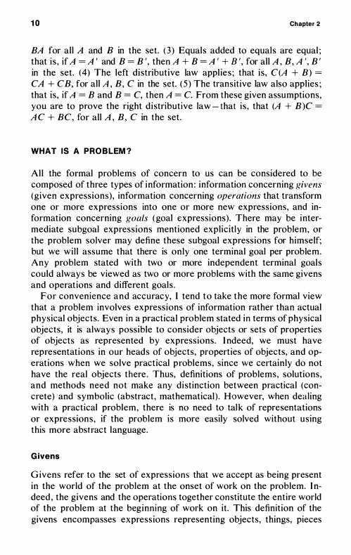
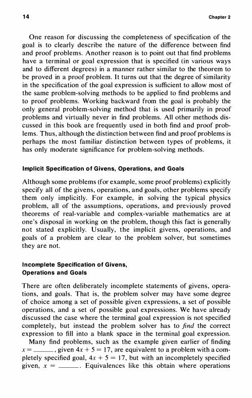
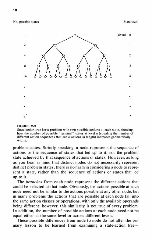
Although the solution of a problem can be defined in terms of either a sequence of actions or a sequence of states (terminating with the achievement of the goal) , it is very useful to represent both the pos­sible sequences of actions and the possible sequences of states in a common diagram, which cou ld be called a state-action tree for a prob­lem. An example of such a tree is shown in Fig. 2-3 .

I n a state-action tree, the nodes or branch points of the tree represent all the possibly different problem states that could result from al l the different action sequences. The concept of a node in a state-action tree differs from the concept of a problem state in a somewhat subtle, but important, way. To be sure , every node represents a state of the prob­lem, but two distinct nodes do not necessari ly represent two distinct or different states of the problem. That is, two or more action se­quences , which result in two different nodes, may result in two identical

18

No. possible states State level

(given ) 0

2

4 2

8 3

16 4

FIGURE 2-3 State-action tree for a problem with two possible actions at each state, showing how the number of possible "terminal" states at level n (equaling the number of d ifferent action sequences that are n actions in length) increases geometrical ly with n.

problem states . Strictly speaking, a node represents the sequence of actions or the sequence of states that led up to it, not the problem state achieved by that sequence of actions or states . However, as long as you bear in mind that distinct nodes do not necessarily represent di stinct problem states , there is no harm in considering a node to repre­sent a state , rather than the sequence of actions or states that led up to i t .

The branches from each node represent the different actions that could be selected at that node. Obvious ly, the actions possible at each node need not be similar to the actions possible at any other node, but in many problems the actions that are possible at each node fal l into the same action classes or operations, with only the avai lable operands being different ; however, this similarity is not true of every problem. I n addition, the number of possible actions at each node need not be equal either at the same level or across different levels .

These possible differences from node to node do not alter the pri­mary lesson to be learned from examining a state-action tree -

Problem Theory 19

namely, how rapidly the number of possible nodes or action sequences increases in such a tree as a function of level , that is , the length of the prior action sequence. If m actions occur at each node, then there are mil possible action (or state) sequences terminating at level n. Each of these different action (state) sequences is represented by a node at level n in the state-action tree, so there are mil different nodes at level n .

This geometric (discrete exponential) increase i s perhaps the single most important fact to consider in developing problem-solving methods . To solve a problem you must state the exact sequence of actions (states) that results in the goal , and many problems require a moder­ately long sequence of actions to accomplish the goal . Thus , we are often faced with a search among an extremely large number of al­ternative action sequences. In these cases , we must "prune the tree" so that there are not so many possible action sequences to investi­gate. But, of course , we must prune in such a manner that we do not cut off all the branches that have "fruit ," that i s , states including the goal .

If you had no basis for choosing between the alternative action'! at each node, if al l the nodes at all levels represented di stinct states (distinct sets of expressions), and if only one of the states (up to and including level n) included the goal , then there would be no way to prune the tree and reduce the search. However, in most problems, it is possible to prune the tree.

Different sequences of actions often result in equivalent problem states, allowing you to combine nodes, prune branches, construct equivalent reduced state-action trees, and so on (for example, classi­ficatory trial and error and macroaction in Chapter 4). U sually, there are good reasons for choosing certain actions at any node and ignor­ing other actions and the branches they generate (for example , state evaluation and hill cl imbing in Chapter 5) . Frequently, a large problem can be broken up into subproblems, thereby transforming a large tree into several smal ler trees , with a great reduction in the total number of branches (for example, subgoal s in Chapter 6) . Sometimes , a much smaller tree results from trying to get from the goal back to the givens, rather than the reverse (for example, working backward in Chapter 8).

Problems with mUltiple given states can be represented by as many state-action trees as there are possible given states . In some problems, the principal task i s to choose among the given states (alternative sets of givens), the one or more given states whose state-action trees con­tain a goal state . Often these problems require only a very short action sequence to achieve the goal , once the correct given state has been selected. In such problems, the main difficulty is to find the correct type of tree in a large forest ; cl imbing the tree may pose only a minor

20 Chapter 2

problem. The method of contradiction discussed in Chapter 7 is often useful for these problems.

There i s a special case of problems with mu ltiple given states that occurs quite frequently and is of particular interest. In these prob­lems, the solver has the option of considering state A to be given and state B to be the goal or of considering state B to be given and state A to be the goal . This kind of equivalence between two problems occurs where inverse operations exist for al l operations . One problem of this type was discussed earl ier in the chapter- namely, the equivalence of deriving x = 3 from 4x + 5 = 1 7 or vice versa.

3

Inference

Virtual ly al l problems present some of the relevant information in impl icit, rather than expl ic it , form. That is , some of the information concerning givens, operations, or occasional ly even goal s is presented in a subtle manner that may not strongly attract your attention, unless you know what to look for. In a sense, this situation might be said to be poor communication of the components of a problem. Why do not the people who make up problems simply do a better job of communi­cating the relevant information?

I would agree that, in some cases , problems used for teaching pur­poses could be improved by making the relevant information very clear. I n these cases the problem is difficult enough in explicit form without the added difficulty of the relevant information being presented im­pl icitly. However, when you are posing and solving mathematical , scientific , and engineering problems for yourself in some real-l ife en­deavor, your own initial posing of problems wil l contain implicit statements of information. U nless you know how to analyze a problem for implicit information, you wil l have difficulty solving actual prob­lems later on.

Problems often evolve from (a) vaguely formulated to (b) semi­precisely formulated to (c) prec isely but partly implicit ly formulated

22 Chapter 3

to (d) precisely and explicitly formulated stages . It is very important for problem solvers to know what kinds of implicit information to look for in problems, because thi s information is often a critical step in problem solving, whether in school or in l ife . Furthermore , even when all the givens and operations are explicit ly presented in the problem, it is, of course, necessary to transform the givens by means of the operations in some way in order to solve the problem. The solver must make inferences, draw conclusions, from the given information, a process that i s , in essence, rendering explicit the statements that were ( in a somewhat different sense) only implicit in the givens.

When implicit information refers to the consequences of given in­formation , it is a somewhat different use of the term than when it refers to information not contained in the explicit statement of the problem (although, by convention, one i s supposed to know that it i s part of the information in the problem). However, there are all degrees of explicit mention of implicit information found in different problems. For example, a problem might refer to even numbers. In one sense, this statement i s explicit mention of even numbers from which one can draw the inference that, if n is an integer and an even number, then it can be expressed as 2m, where m is also an integer. However, the definition of even numbers is not presented explicitly in the prob­lem and must be supplied from memory. This sort of semiexplicit, semi implicit presentation of information occurs all the time in prob­lems. Thus, it is probably not too useful to distinguish between the drawing of conclusions from different degrees of implicitly versus ex­pl icitly presented information.

Drawing inferences from implicit ly or explicit ly presented informa­tion is essential ly random trial and error, unless some criteria are specified regarding which inferences (more generally, which trans­formations of the goal or the given information) should be made first. There are essential ly two criteria that can be formulated semiprecisely, but not completely precisely, at the present time. The first criterion is that the inferences should be those that you have frequently made in the past from the same type of information. You assume that the properties that proved useful in the past wil l most l ikely prove useful in the present problem. The second criterion is that the inferences you draw should be those inferences that are concerned with properties mentioned in the goal , the givens, or in previously derived conse­quences of the goal or the givens. I nferences that sati sfy this second criterion are l ikely to combine with other information to yield sti l l further inferences.

Inference 23

Thus, the general problem-solving method described in this chapter may be stated as follows : Draw inferences from explicitly and implicitly presented information that sa tisfy one or both of the following two criteria: (a) the inferences have frequently been made in the past from the same type of information; (b) the inferences are concerned with properties ( variables, terms, expressions, and so on) that appear in the goal, the givens, or inferences from the goal and the givens. Throughout the rest of the book, the expression "drawing inferences" wil l be used to refer to the above statement of the method - namely, drawing inferences that sati sfy one or both of the previously stated criteria.

Drawing inferences (more general l y, making transformations of the goal or the givens) is probably the first problem-solving method you should employ in attempting to solve a problem. You are essential ly expanding the goal or the givens by bringing to bear a l l of the knowl­edge you have concerning this problem in your memory. Frequently, problems are quite simply solved, once all the relevant information is retrieved from memory, in the drawing of inferences from expl icit ly and implicitl y presented information. Most people do make frequent use of the inference method , at least in connection with drawing inferences from givens. (This procedure is often thought to be random trial and error, but this characterization is largely inaccurate , s ince people 's inferences usual ly do meet one or both of the stated criteria.) The general problem-solving methods discussed later in the book are somewhat less universal l y used by human problem solvers , but the discussion of them should not lead you to ignore the basic inference method. For this reason, this method i s the first general problem­solving method discussed in this book. Furthermore , a greater under­standing of how the inference method operates and an awareness of some i l lustrative use can greatly faci l i tate your proficiency in us ing the method, particularly with respect to inferences from the goal information, which people do not pay enough attention to. People have a bias to start at the beginning, which they take to mean the givens. This bias is often inappropriate in problem solving, s ince the goal is frequently a better beginning point than the givens .

So-called insight problems are often problems in which the principal step in solution is to draw the appropriate inference from certain ex­pl icit ly or impl icitl y presented information. Very few steps are required to solve the problem. What is necessary i s to make that one critical transformation of the givens that essential l y solves the problem. Difficult insight problems are often difficul t precise ly because they

24 Chapter 3

require you to draw an inference that is not too close to the top of your hierarchy of inferences from this type of given information [cri­terion (a)] . Obvious ly, the more you have stored in your memory con­cerning the principal inferences to be drawn from the types of given information contained in the problem, the more l i kely you are to be able to achieve the critical insight . However, whatever your level of specific knowledge concerning the given information, greater under­standing and experience in the u se of the inference method wil l in­crease your chances of systematical l y discovering the required insight in the course of drawing inferences concerning properties of the given information. Just knowing that what you are doing i s surely not random trial and error may cause you to go further and further down the l i st of inferences to be made from the information in the problem, rather than giving up this approach after the first few inferences fai l . With the knowledge of problem-solving methods contained in this book and experience in applying them to the solu tion of problems, you can gradual l y develop a fairly accurate intuition as to which problems are insight problems and thus most suited to the inference method and not to other problem-solving methods . If you c lassify a problem as an insight problem, then you should continue drawing inferences (rather than use other methods) for a longer period of time than if you do not c lass ify it as an insight problem.

Of course, drawing inferences ( including explicit representation of implicit information) is often an important part of solving any problem, not just insight problems. I nsight problems are simply those in which inference is the principal or only method employed in solv ing them. In noninsight problems, you shou ld stop u sing the inference method when you "run out of gas" using the method - that is , when you find it difficult to draw from the given information any new conc lusions that seem to have any l ike l ihood of being u sefu l in solving the problem. I n noninsight problems, you should then go on to consider employing other general problem-solving methods , using the expanded set of given information provided by the inference method . I n insight prob­lems, when you run out of gas , you should go back and try over and over again to look at the problem from a different point of view to yield additional new inferences.

The discussion of inference and implicit information natural ly divides into three sections . F irst, givens may be, to some extent, stated im­pl icitl y and , in any event, can usual ly be expanded considerably by use of the inference method . Second , operations are not always ex­plicit ly stated. Third , the goal of the problem is occasional ly not

Inference 25

completely clear, and the solver must get a precise and correct defini­tion of the goal . In addition , it is often helpful to specify the proper­ties of the goal in more detai l . This procedure frequently involves drawing inferences from presented information (givens and goal ) , including explicit symbolic or diagrammatic representation of informa­tion that may appear only implicitly in the problem.

GIVENS

The problems at the end of a section in a textbook are there to test the reader's knowledge of the material presented in that section. Each problem, then, includes all of the given assumptions, proved theorems, and operations that appeared in the section as wel l as the particular givens of the particular problem. In addition, some previou s material presented in the book may be relevant to solv ing the problem, and certain background knowledge from other books may also be needed. Such background information concerning givens and operations is one kind of implicit information in problems.

You should be aware of this kind of implicit information in prob­lems, and take care to master background subject matter before pro­ceeding on to courses that have this background as a prerequisite. If you have not ful ly understood what was presented previously in the course or what was presented in relevant background courses, you should face this fact and go back to learn the relevant prior material , either simultaneously with or instead of taking a subsequent course. It is lunacy to go on to more advanced courses without a reasonably clear understanding of the relevant background material . The general problem-solving methods taught in this book wil l not substitute for lack of the relevant knowledge.

I t is true that you can understand the relevant material and not be able to solve problems for lack of understanding of general problem­solving methods . However, you wil l al so fail to solve problems if you lack the relevant knowledge , no matter how skil lful a problem solver you are. In today ' s schools a C or even a B in a course may represent an inadequate level of understanding for going on to more advanced courses, and the conscientiou s student should recognize this fact and act accordingly.

In addition to background information, there i s another kind of im­plicit problem information that the skil led problem solver can come to recognize rather easily, sometimes greatly faci l itating solution. This

26 Chapter 3

other kind of implicit information concerns the properties possessed by each of the givens or operations in a problem. When a fami liar object or activity i s presented in a problem, all of the known proper­ties of that object or activity ( including all its known relations to other objects or activities) are usual ly considered to be part of the given in­formation. There may be no question that everyone who works on the problem knows all of the relevant properties of all the givens and operations in the problem. That i s , no specialized background knowl­edge i s required. However, amateur problem solvers frequently fail to ask themselves what they know about the givens and operations in a problem from their own past experience. I nsight problems are very often problems that require one to notice - which means represent explicit ly - properties of givens presented in the problem.

Of course, many of the implicit properties of the givens are irrelevant to solving the problem. We know that most people have two legs, two arms, two eyes, skin, hair, a nose, a mouth, and so on, but most of these properties are irrelevant to the solution of any single problem where people are included in the given information. Such irrelevant properties should be ignored , and problem solvers are usual ly able to reject such tru ly irrelevant implicit properties. The difficulty usual ly comes in abstracting or consciously considering the possibly relevant implicit properties. Some examples are described in the fol lowing subsections .

Numerical Properties

Whenever numbers are involved in a problem in any way, you should consider whether the known properties of the kind of numbers involved in the problem might be of any value in solving the problem. For ex­ample, if some number i s known to be a positive integer, then it cannot be negative, zero, or a fraction . If an integer, n , i s known to be even, then it can be expressed as n = 2m, where m is also an integer, or as n = 2sp, where s i s an integer and p i s an odd integer. If an integer, n, is known to be odd , then it can be expressed as n = 2m + 1 , where m is an integer, or n = 2sp + I , where s is an integer and p is an odd integer.

A somewhat famous example in the psychology of problem solving of the abstraction of numerical properties comes in the J 3 problem of Karl Duncker ( 1 945 , p. 3 1 ) . The problem can be stated as fol lows :

Prove that al l six-place numbers of the form abcabc (for example, 4 1 64 1 6 or 258258) are div is ib le (evenly) by 1 3 .

Inference 27

Stop reading and try to solve this problem, then read on. You might try a variety of special cases , verifying that in every case

the number was divis ible by 1 3 , but that would probably not suggest how to prove the theorem in general . The critical step is to inquire whether you know any numerical properties of a number of the form abcabc. If you could not sol ve this problem before , stop reading and try again by abstracting numerical properties of numbers of the form abcabc.

I f you sti l l cou ld not solve the problem, consider whether you could factor a number of the form abcabc into a product of other numbers. Now stop reading and try again .

I n factoring the number, you no doubt determined that abcabc = (abc) ( \ 00 I ) , for all numbers of the form abc and therefore for al l numbers of the form abcabc. Now, of course, 1 00 1 is d iv isible (evenly) by 1 3 , so (abc) ( 1 00 I ) i s divis ible by 1 3 , and the theorem is proved .

Furthermore , the factoring of abcabc into abc( 1 00 1 ) can be achieved qui te automatical ly by representing the numerical propert ies of abcabc in the fol lowing standard way (for which abcabc i s real l y the conven­tional abbreviation) :

abcabc = (a . 1 05) + (b · 1 04) + (c · l O:l) + (a . 1 02) + (b · 1 0) + (c)

= { / . ( 1 05 + 1 02) + b ( l 04 + 1 0) + c ( l 03 + I )

= a . 1 02 ( l O:l + I ) + b . 1 0( 1 03 + I ) + c t l O3 + I )

= ( l OO I ) (a · 1 02 + b · 1 0 + c ) = ( 1 00 1 ) (abc)

Topological Properties

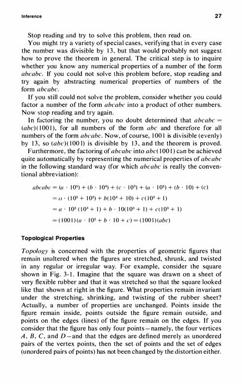
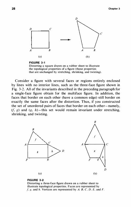
Topology is concerned with the properties of geometric figures that remain una ltered when the figures are stretched, shrunk, and twi sted in any regular or irregular way. For example, consider the square shown in Fig. 3 - 1 . Imagine that the square was drawn on a sheet of very flexible rubber and that it was stretched so that the square looked l ike that shown at right in the figure . What properties remain invariant under the stretching, shrinking, and twisting of the rubber sheet? Actual l y, a number of properties are unchanged . Points inside the figure remain inside, points outside the figure remain outside, and points on the edges ( l ines) of the figure remain on the edges . I f you consider that the figure has only four points - namely, the four vertices A , B , C , and D - and that the edges are defined mere ly as unordered pairs of the vertex points, then the set of points and the set of edges (unordered pairs of points) has not been changed by the di stortion either.

28

D C

D A

(a)

FIGURE 3-1

B

D

C

(b )

Distorting a square drawn on a rubber sheet to i l lustrate the topological properties of a figure (those propert ies that are unchanged by stretching, shrinking, and twisting).

Chapter 3

Consider a figure with several faces or regions entire ly enclosed by l ines with no interior l ines , such as the three-face figure shown in Fig. 3-2 . Al l of the invariants described in the preceding paragraph for a single-face figure obtain for the mult iface figure . I n addition, the faces that border on each other (have a common edge) sti l l border on exactly the same faces after the distortion. Thus , if you constructed the set of unordered pairs of faces that border on each other- namely, if, g) and (g, h ) - this set would remain invariant under stretching, shrinking, and twisting.

B

B

A (-------"t-:. A f------iI C

D

D (a) ( b)

FIG U R E 3-2 D istorting a three-face figure drawn on a rubber sheet to i l lustrate topological properties. Faces are represented by

f, g. and h . Vertices are represented by A. B. C . D . E. and F.

Inference 29

One of my favorite problems involves the property of the bordering (direct connection) of faces in an important way. This i s the no(ched­checkerboard problem :

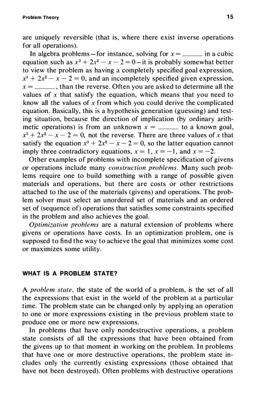
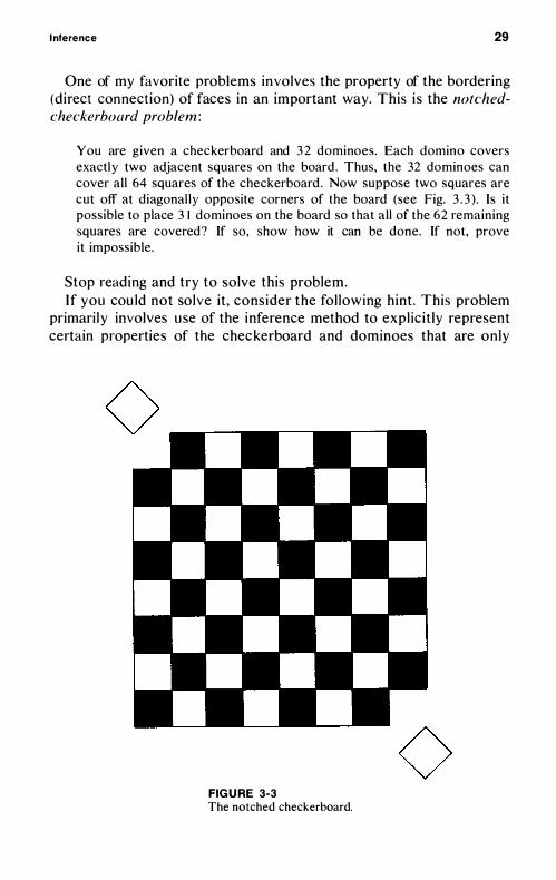
You are given a checkerboard and 3 2 dominoes. Each domino covers exactly two adjacent squares on the board . Thus, the 32 dominoes can cover al l 64 squares of the checkerboard . Now suppose two squares are cut off at diagonal ly opposite corners of the board (see Fig. 3 . 3 ) . Is i t possible to place 3 I dominoes on the board so that al l of the 62 remaining squares are covered? If so, show how it can be done. If not, prove it impossible.

Stop reading and try to solve this problem. I f you cou ld not solve it, consider the fol lowing hint. This problem

primaril y involves u se of the inference method to expl icitly represent certain properties of the checkerboard and dominoes that are only

FIGURE 3-3 The notched checkerboard.

30 Chapter 3

implicitly presented in the present problem. Once the appropriate property or properties are recognized , the solution to the problem is obvious . Now stop reading and try to solve the problem, if you could not do so before .

The critical property is that of the two squares of the checkerboard that are covered by any domino. What are some of the properties of any such two squares? If you have not yet solved the problem, stop reading and try again, considering this hint.

The critical properties of the two squares covered by any domino can be expressed in terms of the colors of these two squares . What are the colors of the two squares covered by any domino on a checkerboard? I f you have not yet solved the problem, stop reading and try again, considering this hint.

The key insight required to solve the notched-checkerboard problem is to notice that a domino covers two squares that are always of different colors (that is , one black and one white). Since the diagonal ly opposite corner squares are of the same color, there are now 30 squares of one color and 32 squares of the other color, and obviously the 62 squares cannot be covered by 3 1 dominoes .

What has intrigued me most about the problem is this : the impos­sibil ity of covering the remaining 62 squares with 3 I dominoes can be proved irrespective of whether the eight-by-eight matrix is presented as a checkerboard with a checkerboard coloring pattern and even irrespective of whether the problem solver has ever experienced a checkerboard coloring pattern. But what problem-solving methcd would lead one to d iscover the elegant proof that comes from imposing a checkerboard coloring pattern on the matrix? Is this kind of ingenious idea a chance happening, or something only very bri l l iant people can think of, using methods that are not understandable by others? I do not think so. I think that use of the problem-solving method of repre­senting all of the possibly relevant properties of the givens in a prob­lem makes it l ikely that many problem solvers would discover the elegant solution of even the notched eight-by-eight colorless matrix problem.

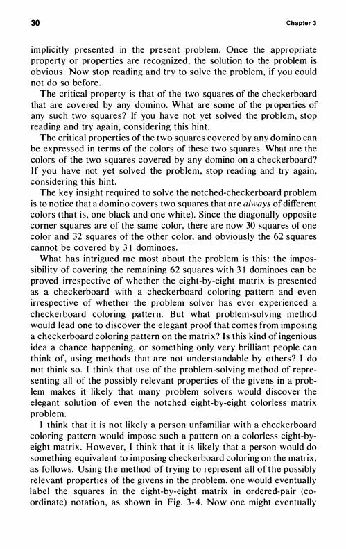
I think that it is not l ikely a person unfamil iar with a checkerboard coloring pattern would impose such a pattern on a colorless eight-by­eight matrix . However, I think that it i s l ikely that a person would do something equivalent to imposing checkerboard coloring on the matrix , as follows. U s ing the method of trying to represent a l l of the possibly relevant properties of the givens in the problem, one would eventual ly label the squares in the eight-by-eight matrix in ordered-pair (co­ord inate) notation, as shown in Fig. 3 -4. Now one might eventually

Inference

o 7 . 1 7,2 7 ,3 7,4 7 , 5 7 ,6 7 , 7

6.0 > , 1 6.2 6,3 6,4 6 ,5 6.6 6,7

5 , 0 5 . 1 5 , 2 5 . 3 5,4 5 .5 5 ,6 5 . 7

4,0 4 , 1 4 , 2 4 , 3 4,4 4 ,'- 4.6 4 ,7

3 , 0 3, 1 3,2 3 .3 3,4 3 .5 3 . 6 3 ,7

2.0 2 , 1 2 ,2 2 , 3 2.4 2,5 2 , 6 2,7

1 , 0 1 . 1 1 , 2 1 .3 1 , 4 1 , 5 1 , 6 1 .7

0,0 0, 1 0.2 0.3 0.4 0,5 0,6

FIGURE 3-4 The notched checkerboard with ordered-pair (coordinate) label ing of the squares.

31

look for some property common to all pairs of squares that a single domino could cover. If the idea occurred to one to look for this kind of property, then having labeled the squares in ordered-pair (coordi­nate) notation, it is likely that one would see that a domino must cover two squares, one of whose coordinate sums is odd and the other even. Since the diagonal ly opposite squares of the matrix both have either an odd or an even coordinate sum, the notched matrix cannot be cov­ered by the 3 1 dominoes. The solution i s in every way equivalent to that given for the notched checkerboard using the color property but in no way requires one to invent some special label ing scheme such as a checkerboard coloring pattern_ Only the very general ly useful and familiar coordinate labeling scheme is needed.

Let us examine why this problem is an example of the abstraction of the topological properties of a figure. A domino covers two faces that border on each other in a complex figure composed of faces with a very special type of bordering structure . It is the bordering structure

32 Chapter 3

of the matrix of faces that is represented by the coordinate labeling scheme (or the checkerboard coloring pattern) , and the shapes and sizes of the faces or the matrix are complete ly irrelevant. Thus , the notched eight-by-eight matrix problem is a problem where the critical properties to be represented are topological properties.

Other problems in which representing topological information is important for achiev ing solution are those in which a block is cut into component subblocks . The fol lowing cube-cutting problem i s , I guess , the c lassic such problem:

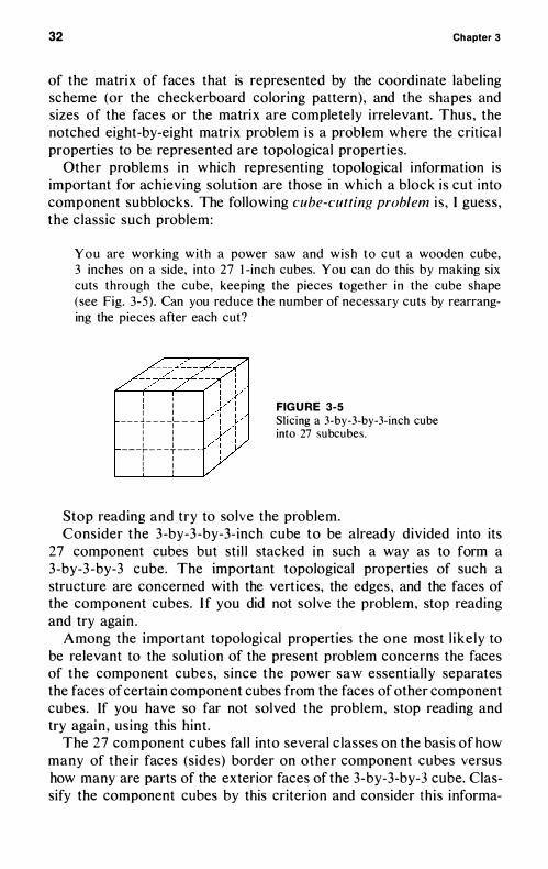
You are working wi th a power saw and wish to cut a wooden cube, 3 inches on a side, into 27 I -inch cubes. You can do this by making six cuts through the cube, keeping the pieces together in the cube shape (see Fig. 3-5) . Can you reduce the number of necessary cuts by rearrang­ing the pieces after each cut?

I I I I

_ _ _ � _ _ _ _ L _ _ I I I I I I I I - - - r - - - T - - -

I I I I I I

FIGURE 3-5

Slicing a 3-by-3-by-3-inch cube into 27 subcubes .

Stop reading and try to solve the problem. Consider the 3 -by-3 -by-3-inch cube to be already divided into its

27 component cubes but sti l l stacked in such a way as to form a 3 -by-3 -by-3 cube. The important topological properties of such a structure are concerned with the vertices, the edges , and the faces of the component cubes. I f you did not solve the problem, stop reading and try again .

Among the important topological properties the one most l ike ly to be relevant to the solution of the present problem concerns the faces of the component cubes, s ince the power saw essential ly separates the faces of certain component cubes from the faces of other component cubes. If you have so far not solved the problem, stop reading and try again , us ing this hint.

The 27 component cubes fal l into several c lasses on the basis of how many of their faces (sides) border on other component cubes versu s how many are parts of the exterior faces of the 3-by-3-by-3 cube. Clas­sify the component cubes by this criterion and consider th is informa-

Inference 33

tion in relation to the solution of the problem. If you have not solved the problem thus far, stop reading and try again .

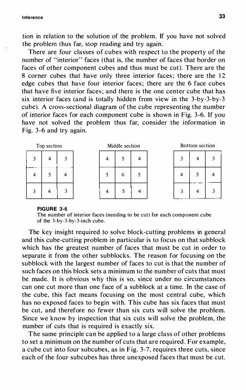
There are four classes of cubes with respect to the property of the number of "interior" faces (that is, the number of faces that border on faces of other component cubes and thus must be cut) . There are the 8 corner cubes that have on ly three interior faces ; there are the 1 2 edge cubes that have four interior faces ; there are the 6 face cubes that have five interior faces ; and there i s the one center cube that has six interior faces (and is total l y hidden from view in the 3 -by-3-by-3 cube). A cross-sectional diagram of the cube representing the number of interior faces for each component cube is shown in Fig. 3 -6. If you have not solved the problem thus far, consider the information in Fig. 3 - 6 and try again .

3

4

3

Top section Middle section Bottom section

4 3 4 5 4 3 4

5 4 5 6 5 4 5

4 3 4 5 4 3 4

FIG U R E 3-6 The number of interior faces (needing to be cut) for each component cube of the 3-by-3-by-3-inch cube.

3

4

3

The key insight required to solve block-cutting problems in general and this cube-cutting problem in particular is to focus on that subblock which has the greatest number of faces that must be cut in order to separate it from the other subblocks . The reason for focusing on the subblock with the largest number of faces to cut is that the number of such faces on this block sets a minimum to the number of cuts that must be made. I t is obvious why this is so, since under no circumstances can one cut more than one face of a subblock at a time. In the case of the cube, this fact means focusing on the most central cube, which has no exposed faces to begin with. This cube has s ix faces that must be cut, and therefore no fewer than six cuts wil l solve the problem. Since we know by inspection that s ix cuts wil l solve the problem, the number of cuts that is required is exactly s ix .

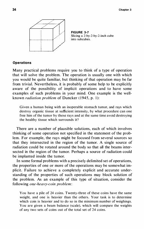
The same principle can be applied to a large c lass of other problems to set a minimum on the number of cuts that are required . For example, a cube cut into four subcubes , as in Fig . 3 -7 , requires three cuts, since each of the four subcubes has three unexposed faces that must be cut.

34

I I I I I I - - - - - - +- - - - - -I I I I I :

FIG U R E 3-7 Slic ing a 2-by-2-by-2-inch cube into subcubes .

Chapter 3

Operations

Many practical problems require you to think of a type of operation that wil l solve the problem. The operation i s usual ly one with which you would be qu ite famil iar, but thinking of that operation may be far from trivial . Nevertheless, it is probably of some help to be explicitly aware of the possibi l ity of implicit operations and to have some examples of such problems in your mind. One example is the well­known radiation problem of Duncker ( 1 945 , p. I ) :

Given a human being with an inoperable stomach tumor, and rays which destroy organic tissue at sufficient intensity, by what procedure can one free him of the tumor by these rays and at the same t ime avoid destroying the healthy tissue which surrounds it?

There are a number of plausible solutions, each of which involves thinking of some operation not specified in the statement of the prob­lem. For example, the rays might be focused from several sources so that they intersected in the region of the tumor. A single source of radiation could be rotated around the body so that all the beams inter­sected in the region of the tumor. Perhaps a source of radiation could be implanted inside the tumor.

I n some formal problems with a precise ly del imited set of operations, the properties of one or more of the operations may be somewhat im­plicit . Fai lure to achieve a completely explicit and accurate under­standing of the properties of such operations may block solution of the problem. As an example of this type of situation, consider the fol lowing one-heavy-coin problem :

You have a pi le of 24 coins . Twenty-three of these coins have the same weight, and one i s heavier than the others . Your task is to determine which coin i s heavier and to do so in the min imum number of weighings. You are given a beam balance (scale), which wil l compare the weights of any two sets of coins out of the total set of 24 coins .

Inference 35

Stop reading and try to solve the problem. Consider the properties of the weighing operation if a beam balance i s used. What kind of in­formation does the beam balance provide concerning relative weights in any two sets of coins? How many different outcomes are there to a weighing on a beam balance? I f you have not solved the problem thus far, stop reading and try again.

A beam balance actual ly has three different outcomes , not two ­namely, the left pan is heavier, l ighter, or equal in weight to the right pan . Since there are three different outcomes to weighing on a beam balance, it is at least theoretical ly possible that a beam balance could provide one with an answer as to which of three subsets of coins con­tains the heavy coin (not just deciding which of two subsets contains the heavy coin) . Consider this h int, and you should easi ly be able to solve the problem.

A beam balance has two pans and compares the weights of two sets of coins. For this reason, many people assume that the operation they have avai lable to solve the problem is essential ly to ask which of two (equal ly large) sets of coins contains the heavy coin. Accordingly, they reason that the optimal strategy must be to divide the total set of coins in half and weigh one half against the other half ( 1 2 coins against 1 2 coins). Then, having determined which set of 1 2 coins contains the heavy coin , they proceed to divide that set in half and weigh 6 coins against 6 coins, then 3 against 3, and final l y I against I , or 2 against 2 followed by I against I .

When the number of coins remaining i s only three , it might occur to a person that one 's original characterization of the operation as a two-way question was in error. However, sometimes even this simple terminal problem does not necessari ly indicate to the problem solver that the beam balance can actual l y provide one with an answer to a three-way question, if the coins are divided into three pi les (two of which are equal) on each and every weighing. This procedure i s , of course , the solution to the problem - namely, you should first weigh two sets of eight coins against each other. If one pan i s heavier than the other, then it contains the heavy coin. If the two pans balance, then the heavy coin i s in the remaining set of eight coins that was left off the pans of the balance scale. I n any case, you find out which subset of eight coins contains the heavy coin . You then continue to partition the remaining set of eight coins into three parts by weighing three coins against three coins. No matter which subset of coins contains the heavy coin , the answer wil l be found in one additional weighing, or three weighings in al l . By contrast, dividing the set into two equal parts (whenever possible) requires four weighings.

36 Chapter 3

I f you are carefu l to explicit ly state the properties of the operations avai lable in a problem, then you will be more l ikely to avoid the in­accurate characterizations that frequently occur in problems such as this one.

GOALS

Occasional ly in school and more frequently in real- l ife problems, the goal of a problem is not completely c lear. Obvious ly, an important step in representing the information in a problem is to be sure you have a precise and correct definition of the goal . I t is often worthwhi le to question whether or not you understood the goal correctly, s ince it is sometimes easy to make a mistake in this regard . As an example, con­sider the fol lowing logic problem:

The country of Marr i s inhabited by two types of people, l iars and truars (truth tellers). Liars always lie and truars always tell the truth. As the newly appointed United States ambassador to Marr, you have been invited to a local cocktail party. While consuming some of the nat ive spirits, you are engaged in conversation with three of Marr's most prominent cit izens : Joan Landi l l , Shawn Farrar, and Peter Gant. At one point in the conversation Joan remarks that Shawn and Peter are both l iars . Shawn vehemently denies that he i s a l iar, but Peter replies that Shawn i s indeed a l iar. From this information can you determine how many of the three are l iars and how many are truars?

Stop reading and try to solve this problem, then read on. In solving logic problems of this type , it is a common procedure to

l i st al l of the possibil it ies in the form of one or more tables. For ex­ample, in this problem one might attempt to fil l out the fol lowing table :

Person

Joan Shawn Peter

Liar Truar

I n a problem very simi lar to this one, a student in one of my problem­solv ing classes attempted to solve the problem by fi l l ing out just such a table . Perhaps you did this in the present problem. However, in translating the problem into this form, a subtle transformation has taken place with respect to the goal - namely, the goal has been changed

Inference 37

from determ in ing hoI\ ' many of the three are l iars to determining whether each of the three persons is a l iar or a truar. If you try to answer the new version of the problem, you wil l never be able to reach a solu tion ! A l l you must determine is how many of the three are l iars. The correct answer is a number: 0 , I , 2 , or 3. The names of the people are largely irrelevant information , added to make the problem appear more interesting and simul taneous ly to act as a distraction. If you have not yet solved the problem, stop reading and try again , then read on.

In fact, it is impossible to determine whether Shawn is a l iar and it is al so impossible to determine whether Peter is a l iar. H owever, one can conclude that either Shawn is a l iar and Peter a truar or Shawn is a truar and Peter a l iar. Either way one and only one of the men i s a l iar. Thus , Joan must be a l iar. This conc lusion implies that there are exact ly two l iars and one truar in the group of three natives to whom you are tal king. This answer solves the original problem but does not al low you to complete ly fill out the table .

In addition to reading and rereading a problem to avoid misunder­standing the goal , you shou ld have a c lear, precise statement of the goal , rather than some vague formulation of it . Sometimes vague state­ments of the goal are partly or completely due to unclear statements of the goal in the problem, and sometimes the vague formulation is due part ly or complete ly to sloppy reformulation by the problem solver. In either case, a vague formulation of the goal may do considerable harm when you attempt to solve a problem. For example , consider the cheap-necklace problem :

You are given four separate pieces of chain that are each three l inks in length. I t costs 2¢ to open a l ink and 3¢ to close a l ink . Al l l inks are closed at the beginning of the problem. Your goal is to obtain a single closed chain , us ing al l l inks , at a cost of no more than 1 5¢ .

The goal is to obtain a single c losed chain , us ing a l l l inks . But what does that mean? I s a single c losed chain a simple loop or circ le? Or would multiple loops be sati sfactory? Is it conceivable that a c losed chain might mean a long chain formed without joining the ends together in a loop? Could there be some other variations on these possibi l ities? U nti l you can decide which of the reasonable possibi l ities constitutes the actual goal of the problem, you do not real ly know what the prob­lem is and cannot expect to make much progress in solv ing it . Some people object to such deliberately vague statements of goals , but vagueness regarding goals is often a feature of real problem solving and you probably should get some experience in deal ing with this kind

38 Chapter 3

of problem. Whether in school or el sewhere , the lesson is that you should be sure you have a precisely formulated and accurate under­standing of the goal .

I n addition to having a prec ise and accurate understanding of the goal , you wil l frequently find it helpful to have a more detailed repre­sentation and understanding of the goal than may be provided in the original statement of the problem. As Polya ( 1 962, p. 7) has empha­sized , it may be useful to imagine for a moment that you have already solved the problem and ask yourself, " What would I have? " Polya variously cal ls th is exercise wishful thinking or taking the problem as solved . Whatever one cal l s this type of thinking, it involves some sort of increase in the expl icit representation of the goal either in sym­bolic (verbal) or diagrammatic form. The usefulness of increasing the specification of the goal may involve l ittle more than introducing names ( labels , symbols) for concepts that appear in the goal but are not explicit ly represented in that form in the original statement of the problem. Thus, one purpose of increasing the specification of the goal is to introduce the necessary working concepts for reaching the goal . Another purpose is to derive some additional properties possessed by the goal , either by rigorous inference from the information contained in the goal and/or the givens of the problem or by representing a rea­sonable conjecture (guess) based on one or another heuristic considera­tion . I n either case, deriving additional properties of the goal may make it easier to reach the goal because then you have a more specific idea of the d ifferent components that you are attempting to achieve.

As an example of a problem where it is useful to represent the goal explicit ly in a diagrammatic form, consider the fol lowing geometry construction problem:

G iven an acute angle U VW and a point P wi th in the angle, use a compass and straightedge to construct a segment QR passing through P, such that QP and PR stand in the ratio 2 : I , Q and R lying on U V and VW, respectively.

In solving this problem, it i s , of course, useful to represent the acute U V W and the point P within the angle as shown in Fig. 3-8 . However, although we do not yet know exactly where point Q l ies on the l ine UV or where point R l ies on the l ine VW, it i s useful to explicit ly repre­sent the goal l ine QR. This representation is done by drawing in a hypothetical dashed l ine, as shown in Fig. 3 -8 . The solution to this problem will be discussed in more detail in Chapter 4, but the advan­tage of explicit representation of the l ine QR is that you are more

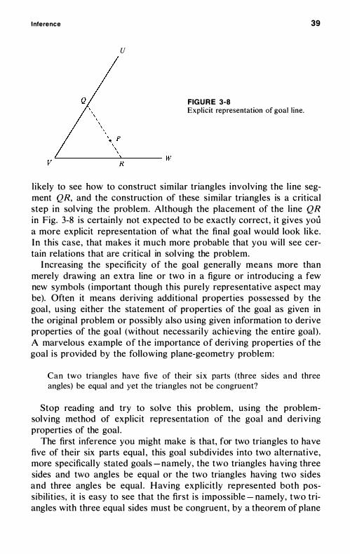
Inference 39

u

FIG U R E 3-8 Explicit representation of goal l ine.

V�----------�

R------- W

l ikely to see how to construct similar triangles involving the l ine seg­ment QR, and the construction of these similar triangles is a critical step in solving the problem. Although the placement of the l ine QR in Fig. 3-8 i s certainly not expected to be exactly correct, it gives you a more explicit representation of what the final goal would look l ike. I n this case, that makes it much more probable that you wil l see cer­tain relations that are critical in solving the problem.

I ncreasing the specificity of the goal general ly means more than merely drawing an extra line or two in a figure or introducing a few new symbols ( important though this purely representative aspect may be). Often it means deriving additional properties possessed by the goal , using either the statement of properties of the goal as given in the original problem or possibly also us ing given information to derive properties of the goal (without necessari ly achieving the entire goal ) . A marvelous example of the importance of deriving properties of the goal i s provided by the following plane-geometry problem:

Can two triangles have five of their s ix parts (three sides and three angles) be equal and yet the triangles not be congruent?

Stop reading and try to solve this problem, us ing the problem­solving method of explicit representation of the goal and deriv ing properties of the goal .

The first inference you might make is that, for two triangles to have five of their six parts equal , this goal subdivides into two alternative, more specifical ly stated goals - namely, the two triangles having three sides and two angles be equal or the two triangles having two sides and three angles be equal . Having explicit ly represented both pos­sibil it ies, it is easy to see that the first i s impossible - namely, two tri­angles with three equal sides must be congruent, by a theorem of plane

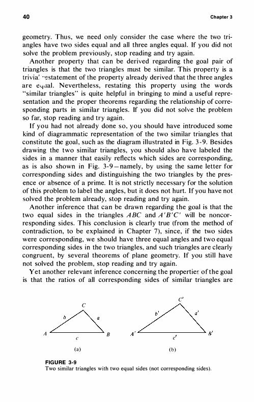
40 Chapter 3

geometry. Thu s, we need only consider the case where the two tri­angles have two sides equal and all three angles equal . If you did not solve the problem previously, stop reading and try again .

Another property that can be derived regarding the goal pair of triangles is that the two triangles must be similar. This property is a triv ia� ··t;!statement of the property already derived that the three angles are e'-tiJal . Nevertheless, restating this property using the words "s imilar triangles" is quite helpful in bringing to mind a useful repre­sentation and the proper theorems regarding the relationship of corre­sponding parts in simi lar triangles . If you did not solve the problem so far, stop reading and try again .

I f you had not already done so , you should have introduced some kind of diagrammatic representation of the two similar triangles that constitute the goal , such as the diagram i l lustrated in Fig. 3 - 9 . Besides drawing the two similar triangles, you should also have labeled the sides in a manner that easi l y reflects which sides are corresponding, as i s also shown in Fig. 3 -9 - namely, by using the same letter for corresponding sides and distinguishing the two triangles by the pres­ence or absence of a prime. It is not strictly necessary for the solution of th is problem to label the angles , but it does not hurt. If you have not solved the problem already, stop reading and try again .

Another inference that can be drawn regarding the goal is that the two equal sides in the triangles A Be and A ' B ' C ' will be noncor­responding sides. This conclusion is clearly true (from the method of contradiction, to be explained in Chapter 7) , since, if the two sides were corresponding, we should have three equal angles and two equal corresponding sides in the two triangles, and such triangles are c learly congruent, by several theorems of plane geometry. I f you sti l l have not solved the problem, stop reading and try again .

Yet another relevant inference concerning the propertie� of the goal is that the ratios of all corresponding sides of similar triangles are

c' c

� A B c

(a) (b)

FIGURE 3-9 Two similar triangles with two equal sides (not corresponding sides) .

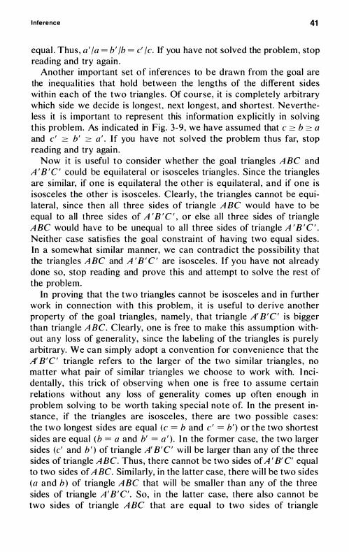
Inference 41

equal . Thus , a ' /a = b ' /b = e' /e. If you have not solved the problem, stop reading and try again .

Another important set of inferences to be drawn from the goal are the inequalit ies that hold between the lengths of the different sides within each of the two triangles . Of course, it is complete ly arbitrary which side we decide is longest , next longest, and shortest. Neverthe­less it i s important to represent this information explicit ly in solving this problem. As indicated in Fig. 3 -9 , we have assumed that e 2': b 2': a and c ' 2': b ' 2': a ' . I f you have not solved the problem thus far, stop reading and try again .

Now i t is u sefu l to consider whether the goal triangles A BC and A ' B ' C ' cou ld be equi lateral or i sosceles triangles . Since the triangles are simi lar, if one i s equilateral the other is equi lateral , and if one i s isosceles the other is i sosceles. Clearly, the triangles cannot be equi­lateral , since then all three sides of triangle A BC would have to be equal to all three sides of A ' B ' C ' , or else al l three sides of triangle A BC would have to be unequal to al l three sides of triangle A ' B ' C ' . Neither case satisfies the goal constraint of having two equal s ides. In a somewhat similar manner, we can contradict the possibi l i ty that the triangles A BC and A ' B ' C ' are isosceles . I f you have not already done so, stop reading and prove this and attempt to solve the rest of the problem.

In proving that the two triangles cannot be isosceles and in further work in connection with this problem, it i s useful to derive another property of the goal triangles, namely, that triangle A' B ' C ' is bigger than triangle A BC. Clearly, one is free to make this assumption with­out any loss of general ity, since the labeling of the triangles is purely arbitrary. We can simply adopt a convention for convenience that the A' B 'C ' triangle refers to the larger of the two similar triangles , no matter what pair of similar triangles we choose to work with. I nci­dental ly, this trick of observing when one is free to assume certain relations without any loss of general ity comes up often enough in problem solving to be worth taking special note of. In the present in­stance , if the triangles are isosceles , there are two possible cases : the two longest sides are equal (c = b and e ' = b ' ) or the two shortest sides are equal (b = a and b' = a ' ) . I n the former case, the two larger sides (e' and b ' ) of triangle A' B ' C ' wi l l be larger than any of the three sides of triangle A BC. Thus, there cannot be two sides of A ' B' C' equal to two sides of A BC. Simi larly, in the latter case, there wi l l be two sides (a and b ) of triangle A BC that wil l be smal ler than any of the three sides of triangle A ' B ' C' . So, in the latter case, there also cannot be two sides of triangle A BC that are equal to two sides of triangle

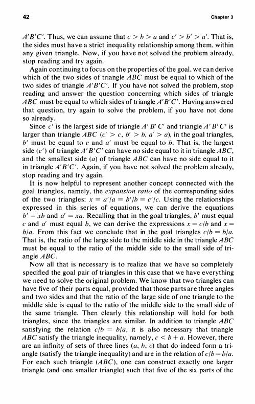
42 Chapter 3

A ' B ' C ' . Thus, we can assume that e > b > a and e ' > b ' > a ' . That is , the s ides must have a strict inequality relationship among them, within any given triangle. Now, if you have not solved the problem already, stop reading and try again .

Again continuing to focus on the properties of the goal , we can derive which of the two sides of triangle A BC must be equal to which of the two sides of triangle A ' B ' C ' . If you have not solved the problem, stop reading and answer the question concerning which sides of triangle A BC must be equal to which sides of triangle A ' B 'C ' . Having answered that question, try again to solve the problem, if you have not done so already.

Since e ' i s the largest side of triangle A I B' C' and triangle A I B ' C' is larger than triangle ABC (e' > e , b' > b, a' > a), in the goal triangles, b ' must be equal to e and a ' must be equal to b. That is, the largest side (e ' ) of triangle A ' B ' C ' can have no side equal to it in triangle A BC, and the smal lest side (a) of triangle A BC can have no side equal to it in triangle A ' B ' C ' . Again , if you have not solved the problem al ready, stop reading and try again .

I t is now helpful to represent another concept connected with the goal triangles, namely, the expansion ratio of the corresponding sides of the two triangles : x = a ' /a = b ' /b = e ' /e. U sing the relationships expressed in this series of equations, we can derive the equations b ' = xb and a' = xa. Recal l ing that in the goal triangles , b ' must equal e and a' must equal b, we can derive the expressions x = e/b and x = b/a. From this fact we conclude that in the goal triangles e/b = b/a. That is, the ratio of the large side to the middle side in the triangle A BC must be equal to the ratio of the middle side to the smal l side of tri­angle A BC.

Now al l that i s necessary is to realize that we have so completely specified the goal pair of triangles in this case that we have everything we need to solv� the original problem. We know that two triangles can have five of their parts equal , provided that those parts are three angles and two sides and that the ratio of the large side of one triangle to the middle side i s equal to the ratio of the middle side to the small side of the same triangle. Then clearly this re lationship wi I I hold for both triangles , since the triangles are s imi lar. In addition to triangle ABC satisfying the relation e/b = bfa , it is also necessary that triangle A BC sati sfy the triangle inequality, namely, c < b + a. However, there are an infinity of sets of three l ines (a , b , e) that do indeed form a tri­angle (satisfy the triangle inequality) and are in the relation of e/b = b/a. For each such triangle (A BC) , one can construct exactly one larger triangle (and one smal ler triangle) such that five of the six parts of the

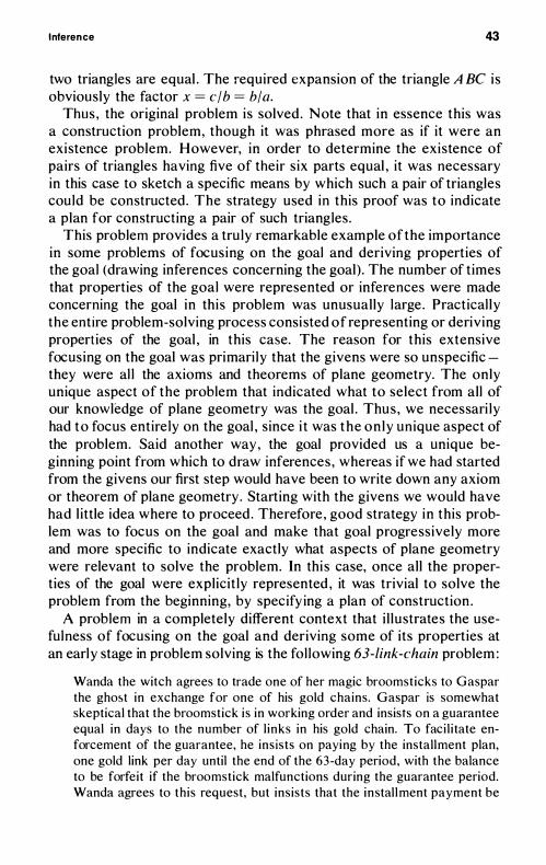
Inference 43

two triangles are equal . The required expansion of the triangle A Be i s obviously the factor x = c/b = b/a.

Thus , the original problem is solved . Note that in essence this was a construction problem, though it was phrased more as if it were an existence problem. However, in order to determine the existence of pairs of triangles having five of their s ix parts equal , it was necessary in this case to sketch a specific means by which such a pair of triangles could be constructed . The strategy used in this proof was to indicate a plan for constructing a pair of such triangles .

This problem provides a tru ly remarkable example of the importance in some problems of focusing on the goal and deriving properties of the goal (drawing inferences concerning the goal) . The number of times that properties of the goal were represented or inferences were made concerning the goal in this problem was unusually large . Practical ly the entire problem-solving process consi sted of representing or deriving properties of the goal , in this case. The reason for this extensive focusing on the goal was primari l y that the givens were so unspecific ­they were al l the axioms and theorems of plane geometry. The only unique aspect of the problem that indicated what to select from all of our knowledge of plane geometry was the goal . Thus , we necessari ly had to focus entire ly on the goal , since i t was the on ly unique aspect of the problem. Said another way , the goal provided us a unique be­ginning point from which to draw inferences , whereas if we had started from the givens our first step would have been to write down any axiom or theorem of plane geometry . Starting with the givens we would have had l ittle idea where to proceed . Therefore , good strategy in this prob­lem was to focus on the goal and make that goal progressively more and more specific to indicate exactly what aspects of plane geometry were relevant to solve the problem. In thi s case, once all the proper­ties of the goal were explicit ly represented , it was trivial to solve the problem from the beginning, by specify ing a plan of construction .

A problem in a completely different context that i l lustrates the use­fulness of focusing on the goal and deriving some of its properties at an earl y stage in problem solving is the fol lowing 63-link-chain problem :

Wanda the witch agrees to trade one of her magic broomst icks to Gaspar the gho!>t in exchange for one of his gold chains . Gaspar is somewhat skeptical that the broomstick i s in working order and insists on a guarantee equal in days to the number of l inks in his gold chain. To faci l i tate en­forcement of the guarantee, he ins ists on paying by the instal lment plan, one gold link per day until the end of the 63-day period, with the balance to be forfeit if the broomstick malfunctions during the guarantee period. Wanda agrees to th is request, but ins ists that the instal l ment payment be

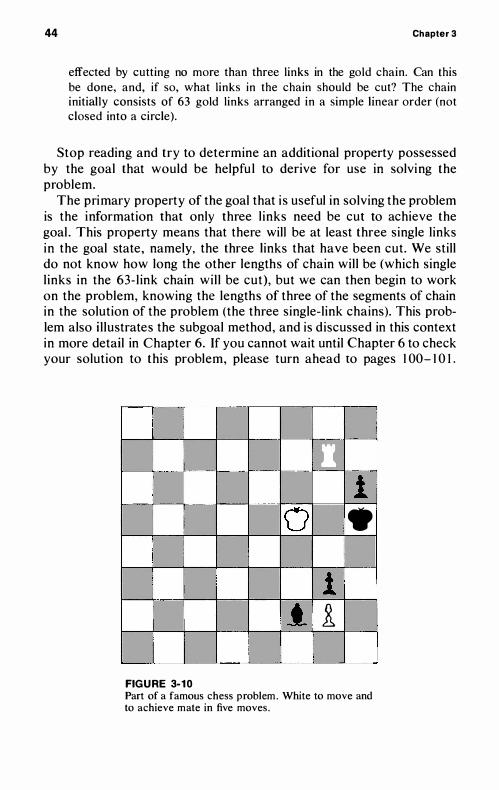
44 Chapter 3

effected by cutting no more than three links in the gold chain. Can this be done, and, if so, what l inks in the chain should be cut? The chain initial ly consists of 63 gold links arranged in a simple linear order (not closed into a circle).

Stop reading and try to determine an additional property possessed by the goal that would be helpfu l to derive for use in solving the problem.

The primary property of the goal that i s useful in solving the problem is the information that only three l inks need be cut to achieve the goal . This property means that there will be at least three single l inks in the goal state , namely, the three l inks that have been cut. We still do not know how long the other lengths of chain wil l be (which single l inks in the 63- l ink chain wi l l be cut) , but we can then begin to work on the problem, knowing the lengths of three of the segments of chain in the solution of the problem (the three single-l ink chains). This prob­lem also i l lustrates the subgoal method, and is d iscussed in this context in more detail in Chapter 6. If you cannot wait until Chapter 6 to check your solution to this problem, please turn ahead to pages 1 00- 1 0 I .

0 1

0 -

1 .t l

FIGURE 3-1 0 Part of a famous chess problem . White to move and to achieve mate in five moves .

Inference 45

I n some problems, one cannot rigorously infer additional properties possessed by the goal , but one can make reasonable conjectures based on heuristic principles. For example, consider the following chess problem, which constitutes one portion of a famous problem originated by Sam Lloyd . The problem is for white to achieve checkmate in five moves from the starting position shown in Fig. 3 - 1 0 . Stop reading and try to solve thi s problem by guessing one or more plaus ible goal posi­tions in which black is checkmated and then try to determine how you could achieve such a checkmate position.

I t seems reasonable to conjecture that the checkmate position will have white 's rook at his own king's rook one. That is, white ' s rook will be at the end of the open file where he has the black king trapped. Black has the potential opportunity to interpose his bishop at two places in that file between the conjectured position of white 's rook and black's king. However, the move sequences by which black can inter­pose his bishop between the white rook and the black king can al l be frustrated by white in one way or another. The essential strategy for solving the chess problem comes by conjecturing that you wish to have the white rook at white ' s king's rook one , without the possibil ity of black blocking the attack by his bishop, and then working forward to determine what white must do at each move in order to achieve that terminal checkmate position.

4

Classification of

Action Sequences

RANDOM TRIAL AND ERROR

The first thing that most people do when confronted with a problem is to start applying the allowable operations to the givens in the problem. Call this random trial and error. (Readers with a course in probability should understand that what I am cal l ing random trial and error is equivalent to random sampling with replacement from the population of action sequences less than or equal to some maximum length . ) If a very short sequence of such actions is sufficient to get from the givens to the goal , even randomly generated sequences of actions may yield the solution fairly quickly.

SYSTEMATIC TRIAL AND ERROR

To avoid going around in circ les , it is obviously desirable to remember what sequences of actions have been tried already with no success. In addition, it i s desirable to have a scheme for systematical ly generat­ing different sequences of actions , which guarantees that all sequences (to some maximum length) will be generated. Most desirable of all random trial-and-error schemes wou ld be a generation method that

Classification of Action Sequences 47

automatical l y produced a mutual ly exclusive and exhaustive l isting of all sequences of actions up to some maximum length. Call this sys­tematic trial and error (equivalent to random sampling without re­placement) .

From the above discussion, it should be relatively obvious that there can be different degrees of systematicness between random and completely systematic trial and error. A problem solver could have some memory for past attempts, but it could be l imited or subject to error. A problem solver could also have different degrees of effective­ness in systematical ly generating all of the different sequences of actions. The degree of systematicness in the use of trial and error is one useful indicator of the intell igence of different species of animals . I th ink it is not known whether any species of animal below human beings can be trained to be more systematic in their trial and error, but humans certainly can be. People can overcome their memory l imitations by writing things down, and they can often invent mutual l y exclusive and exhaustive generation schemes, though the difficulty of accomplishing the latter varies from problem to problem.

CLASSIFICATORY TRIAL AND ERROR

The most powerful kind of trial and error is what might be called classificatory trial and error, which requires that sequences of actions be organized into classes that are equivalent (or probably equivalent) with respect to the solution of the problem. That is, if one sequence of actions within a class will solve the problem, then all the other se­quences of actions within the same class will probably al so solve the problem. Conversely, if one sequence of actions within the class can be shown not to solve the problem, then probably every other sequence of actions in the same class will also fai l .

To appreciate the power of classificatory trial and error, consider a state-action tree with n possible actions at each node of the tree. With this representation, there are nm possible sequences of actions that are m actions in length . For even rather small values of n and m , n m can b e s o large a s to prohibit the use of systematic trial and error.

Obvious ly, if nm sequences of actions could be reduced to a small number of equivalence classes - that is, classes that are equivalent with respect to the solution of the problem - it would make the problem much simpler to solve. In this case , you could systematical ly try one sequence from each class unti l you found a class that solved the prob­lem. Such classificatory trial and error only works for problems where

48 Chapter 4

sequences of actions fal l into classes that are equ ivalent with respect to solution of the problem, but most of the problems people solve probably exhibit some such equivalences.

There are four different categories of problems in which classifica­tory trial and error is helpfu l , and within each four are two subtypes. To d iscuss these types of problems, let us imagine that the states reached by various action sequences applied to the given information can be represented by a sequence of letters , where the first letter stands for the action taken at the first node, the second letter for action at the second node, and so on. Thus , abc represents the state reached by taking action a at the first node, fol lowed by action b at the second node, fol lowed by action c at the third node in the state-action tree. The basic principle i s that two or more action sequences are equivalent if and only if they result in the same state or states thought to be equiva­lent with respect to solving the problem.

The first major type of equivalence class of action sequences i s the obvious one that results from having equivalence c lasses of actions. In this case, for example, let us imagine that a set of actions {b l , b2 , b3 , • • • } = { bi } are all identical or thought to be equivalent. I n this case , the action sequence ab;c i s equivalent to the action sequence abjc, for all i and j. People usual ly have no trouble in identifying equivalence c lasses of action sequences based on such elementary equi­valences of component actions . Such equivalent actions often arise in problems where there are a large number of equivalent givens, such as a large number of entities of the same type - for example, six sticks identical in length and every other important property. When the givens are not identical in every respect but are equivalent with respect only to the properties that are thought to be important to the problem, then recognition of such equivalences may be more difficult and subject to error. In any event, identical or equivalent actions (often resulting from identical or equivalent givens) produce the first type of equiva­lence classes of action sequences.

A second and relatively fami l iar type of equivalence class of action sequences ari ses in problems having commutative actions - that is , where the result of taking action a followed by action b yields the same result as taking action b fol lowed by action a. If three actions (abc) are all commutative with respect to one another, then action sequences abc, acb, bac, bca, cab, and cba are all equivalent, since they result in the same state when applied to the same given information or other starting point in a problem. For example, in solving for x, given the equation 5x + 17 = 3x + 2 1 , we could subtract 3x from both sides of the equation as the first step, then subtract 1 7 from both sides as the

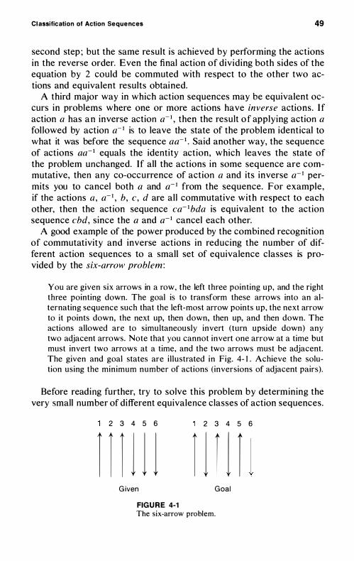
Classification of Action Sequences 49

second step ; but the same result is achieved by performing the actions in the reverse order. Even the final action of dividing both sides of the equation by 2 could be commuted with respect to the other two ac­tions and equivalent results obtained.

A third major way in which action sequences may be equivalent oc­curs in problems where one or more actions have inverse actions. I f action a has an inverse action a- I , then the result of applying action a fol lowed by action a- I is to leave the state of the problem identical to what it was before the sequence aa- 1 • Said another way, the sequence of actions aa-1 equals the identity action, which leaves the state of the problem unchanged. If all the actions in some sequence are com­mutative, then any co-occurrence of action a and its inverse a- I per­mits you to cancel both a and a- I from the sequence. For example, if the actions a, a- I , b , c , d are al l commutative with respect to each other, then the action sequence ca- 1bda is equivalent to the ac tion sequence cbd, since the a and a-I cancel each other.

A good example of the power produced by the combined recognition of commutativity and inverse actions in reducing the number of dif­ferent action sequences to a small set of equivalence classes is pro­vided by the six-arrow problem :

You are given six arrows in a row, the left three pointing up, and the right three pointing down. The goal is to transform these arrows into an al­ternating sequence such that the left-most arrow points up, the next arrow to i t points down, the next up, then down, then up, and then down. The actions al lowed are to s imultaneously invert (turn upside down) any two adjacent arrows. Note that you cannot invert one arrow at a time but must invert two arrows at a time, and the two arrows must be adjacent. The given and goal states are i l lustrated in Fig. 4- 1 . Achieve the solu­tion using the minimum number of act ions ( inversions of adjacent pairs).

Before reading further, try to solve this problem by determining the very small number of different equivalence classes of action sequences.

2 3 4 5 6 2 3 4 5 6

r r r 1 1 1 r 1 r 1 r j G iven Goal

FIG U R E 4-1 The six-arrow problem.

50 Chapter 4

I f you have not solved the problem, consider the fol lowing. I n representing the information given in the problem, you shou ld note that there are only five different possible actions that you can take at any given stage of the problem - namely, to invert arrows I and 2, 2 and 3 , 3 and 4 , 4 and 5 , or 5 and 6 , as shown i n Fig. 4- 1 . Of course , if every different sequence of actions had to be considered , and you had no way of knowing how long a possible sequence might be necessary to solve the problem, then the problem could be extraordinari l y difficult , de­spite the l imited number of actions available at each node. In fact, a l i ttle reasoning concerning the equivalence of different action se­quences reduces the number of nonequivalent action sequences to an extremely smal l number.

I n the first place, you should note that the order in which you per­form the actions makes no difference. That i s , the actions commute one with another, so that inverting arrows 3 and 4 and then inverting 4 and 5 is completely equivalent to first inverting 4 and 5 and then inverting 3 and 4. The same is true for any set of three or more actions in a sequence. Thus , you do not have to deal with ordered sets of ac­tions but only with unordered sets. This statement simply means that al l the dift'erent orderings ( permutations) of a given unordered set of action sequences are equivalent, greatly reducing the number of pos­sible solutions to be considered . Now stop reading and try to solve the problem, if you could not before .

I f you sti l l cannot solve the problem, consider the fol lowing h int. An optimal solution will contain no more than one occurrence of any given type of action. An action is its own inverse. I nverting arrows 2 and 3 twice leaves the arrows exactly the same as they were. Thus, any pair of two occurrences of a given action can be canceled (even if they are not adjacent, since the actions are complete ly commutative). Any even number of occu rrences of an action is equivalent to zero occurrences of that action, and , for the same reason , any odd number of occurrences is equivalent to a single occurrence. Thus , we need consider only combinations (unordered sets) of from one to five pos­sible actions . At this point we have reduced a potential ly infinite num­ber of different action sequences to 3 1 possible classes of action sequences. Each of the 3 1 classes can be represented by its simplest member, as fol lows : 5 single-step actions, 1 0 two-step action sequences, 1 0 three-step action sequences , 5 four-step action sequences , and 1 five-step action sequence. Stop reading and try to solve the problem, if you did not before .

We can now observe that two of the five actions - namely, inverting arrows 1 and 2 and inverting arrows 5 and 6 - cannot possibly be in­cluded in the optimal solution , since these actions change arrows 1

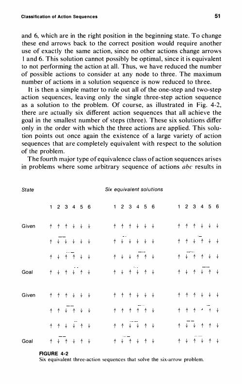
Classification of Action Sequences 51

and 6, which are in the right position in the beginning state . To change these end arrows back to the correct position would require another use of exact ly the same action, since no other actions change arrows I and 6. This solution cannot possibly be optimal , since it i s equivalent to not performing the action at al l . Thus, we have reduced the number of possible actions to consider at any node to three . The maximum number of actions in a solution sequence i s now reduced to three.

I t i s then a simple matter to ru le out all of the one-step and two-step action sequences, leaving only the s ingle three-step action sequence as a solution to the problem. Of course, as i l lustrated in Fig. 4-2, there are actual ly six different action sequences that all achieve the goal in the smal lest number of steps (three) . These s ix solutions differ only in the order with which the three actions are applied. This solu­tion points out once again the existence of a large variety of action sequences that are completely equivalent with respect to the solution of the problem.

The fourth major type of equivalence c lass of action sequences ari ses in problems where some arbitrary sequence of actions abc results in

Sta te Six equivalent solutions

1 2 3 4 5 6 1 2 3 4 5 6 1 2 3 4 5 6

G iven t t t + + + t t t + + + t t t + + +

t + + + + + t + + + + + t t + t + +

t + t t + + t + + t t + t + t t + +

Goal t + t + t + t + t + t + t + t + t +

G iven t t t + + + t t t + + + t t t + + +

t t + t + + t t t t t + t t t t +

t t + + t + t t + + t + t + + t t +

Goal t + t + t + t + t + t + t + t + t +

RGURE 4-2 Six equivalent three-act ion sequences that solve the s ix-arrow problem.

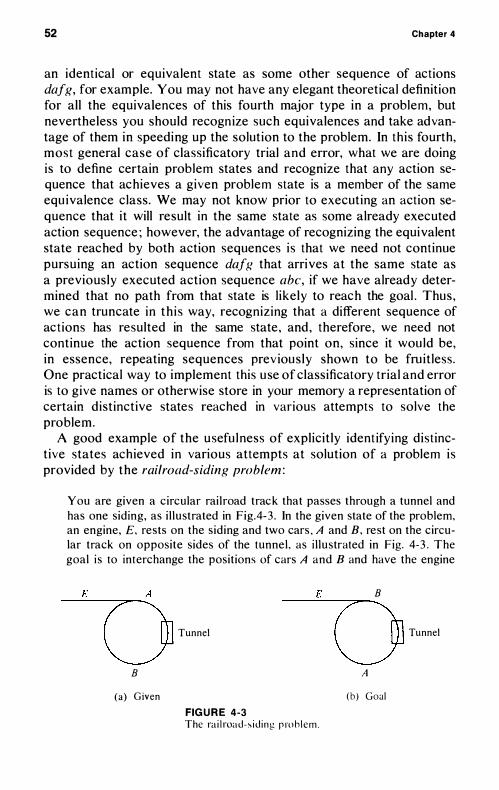
52 Chapter 4

an identical or equivalent state as some other sequence of actions dafg, for example. You may not have any elegant theoretical definition for all the equivalences of this fourth major type in a problem, but nevertheless you should recognize such equivalences and take advan­tage of them in speeding up the solution to the problem. In th is fourth, most general case of classificatory trial and error, what we are doing is to define certain problem states and recognize that any action se­quence that achieves a given problem state is a member of the same equ ivalence class . We may not know prior to executing an action se­quence that it will result in the same state as some already executed action sequence ; however, the advantage of recognizing the equivalent state reached by both action sequences is that we need not continue pursuing an action sequence dafg that arrives at the same state as a previously executed action sequence abc, if we have already deter­mined that no path from that state is l ikely to reach the goal . Thus , we can truncate in th is way, recognizing that a different sequence of actions has resulted in the same state , and , therefore , we need not continue the action sequence from that point on, since it wou ld be, in essence, repeating sequences prev iou sly shown to be fru it less. One practical way to implement this u se of classificatory trial and error is to give names or otherwise store in your memory a representation of certain distinctive states reached in various attempts to solve the problem.

A good example of the usefu lness of explicitly ident ifying distinc­tive states ach ieved in various attempts at solution of a problem is provided by the railroad-siding problem :

You are given a circular rai l road track that passes through a tunnel and has one siding, as i l lustrated in Fig.4-3 . In the given state of the problem, an engine, E, rests on the s iding and two cars , A and B, rest on the circu­lar track on opposite sides of the tunnel , as i l lustrated in Fig. 4-3 . The goal i s to interchange the posit ions of cars A and B and have the engine

B

Tunnel Tunnel

B A

(a) Given (b) Goal

FIG U R E 4-3 The ra i l roa d - � i d i n g p ro h l e m .

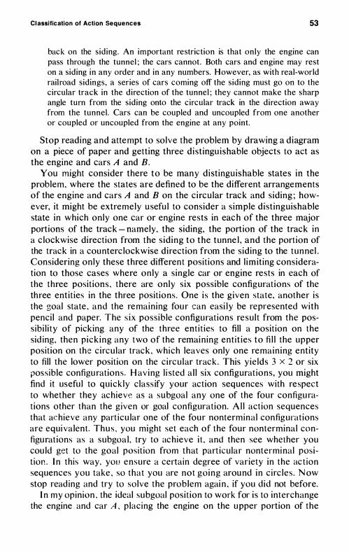
Classification of Action Sequences 53

back on the s iding. An important restrict ion is that only the engine can pass through the tunnel ; the cars cannot . Both cars and engine may rest on a siding in any order and in any numbers. However, as with real-world rail road sidings, a series of cars coming off the s iding must go on to the circular track in the d irection of the tunnel ; they cannot make the sharp angle turn from the s iding onto the circular track in the d irection away from the tunnel . Cars can be coupled and uncoupled from one another or coupled or uncoupled from the engine at any point .

Stop reading and attempt to solve the problem by drawing a diagram on a piece of paper and getting three distingu ishable objects to act as the engine and cars A and B.

You might consider there to be many distinguishable states in the problem, where the states are defined to be the different arrangements of the engine and cars A and B on the circular track and siding ; how­ever, it might be extremely usefu l to consider a simple distinguishable state in which only one car or engine rests in each of the three major portions of the track - namely, the siding, the portion of the track in a c lockwise direction from the s iding to the tunne l , and the portion of the track in a counterc lockwise direction from the siding to the tunnel . Considering only these three different positions and l imiting considera­tion to those cases where only a single car or engine rests in each of the three positions , there are only six possible configurations of the three entities in the three positions . One is the given state, another is the goal state , and the remaining four can easi l y be represented with pencil and paper. The s ix possible configurations resu l t from the pos­sibi l i ty of picking any of the three entit ies to fill a position on the sid ing, then picking any two of the remaining ent i t ies to fi l l the upper position on th·e circu lar track , which leaves only one remaining entity to fill the lower position on the circu lar track . This yie lds 3 x 2 or six possible configu rations . H aving l i sted al l six configurat ions, you might find it usefu l to quick ly class ify your action sequences with respect to whether they achieve as a subgoal any one of the four configu ra­tions other than the given or goal configuration. A l l action sequences that achieve any part icu lar one of the four nonterminal configurations are equivalent . Thu s , you might set each of the four nonterminal con­figurations as a subgoal , try to achieve i t , and then see whether you cou ld get to the goal posit ion from that part icular nonterminal posi­t ion . I n this way, you ensure a certain degree of variety in the ac t ion sequences you take , so that you are not going around in c i rc les . N ow stop read ing and try to solve the problem again , if you did not before.

I n my opinion , the ideal subgoal posit ion to work for is to interchange the engine and car A , placing the engine on the upper portion of the

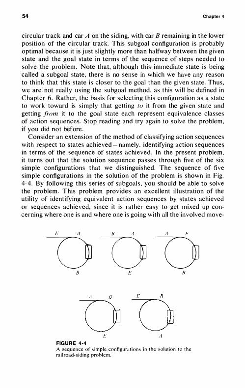
54 Chapter 4

circular track and car A on the siding, with car B remaining in the lower position of the circular track. This subgoal configuration is probably optimal becau se it is just s l ightly more than halfway between the given state and the goal state in terms of the sequence of steps needed to solve the problem. Note that, although this immediate state i s being cal led a subgoal state , there is no sense in which we have any reason to think that this state is closer to the goal than the given state . Thus , we are not real l y using the subgoal method , as this wi l l be defined in Chapter 6. Rather, the basis for selecting this configu ration as a state to work toward is s imply that getting to i t from the given state and getting from it to the goal state each represent equi valence classes of action sequences. Stop reading and try again to solve the problem, if you did not before .

Consider an extension of the method of classifying action sequences with respect to states achieved - namely, identifying action sequences in terms of the sequence of states achieved. In the present problem, it turns out that the solution sequence passes through five of the six simple configurations that we dist ingu ished. The sequence of five simple configurations in the solution of the problem is shown in Fig. 4-4. By fol lowing this series of subgoal s , you should be able to solve the problem. This problem provides an excel lent i l l u stration of the uti l ity of ident ifying equi valent action sequences by states achieved or sequences ach ieved, since i t is rather easy to get mixed up con­cerning where one i s and where one is going wi th all the involved move-

t; A B A A E

D D D B E B

D u E A

FIG U R E 4-4 A sequence of � i m p l e configura t i o n � i n the solut ion to the ra i l road- s id ing problem.

Classification of Action Sequences 55

ments of cars and engines required in order to solve the problem. I f one does not identify landmarks along the way, it i s easy to go around in circ les .

So far, the examples that have been presented have i l lustrated only cases where several different action sequences were considered equiva­lent becau se they achieved precisel y identical states . I n some prob­lems, it i s usefu l to consider action sequences to be equivalent when they ach ieve states that are considered equivalent with respect to solution of the problem, despite the fact these states may not be iden­tical in every respect. The states ( and therefore the action sequences that lead to them) are considered equ ivalent because they al l have cer­tain propert ies in common that we judge to make the states equivalent insofar as solving this particu lar problem is concerned ( though the states might wel l not be judged equivalent with respect to solv ing some other problem) . Such class ificat ion of states (and action sequences) as equi valent is , of course, more dangerous than the complete ly safe classification of states as equivalent when the states are identica l . I f our judgment i s fau l ty concerning which properties are relevant and irrelevant to the solution of the problem, then our judgment that all members of some equivalence class wi l l fai l to sol ve the problem may be fau lty. N evertheless , our judgment concerning relevant and ir­relevant properties is general l y sufficientl y good that such equivalence c lasses are general l y quite usefu l . An example of th is type of equiva­lence classification of action sequences along with some of the identity­based equi valence c lass ification of action sequences i s provided by the cheap-neck lace problem :

You are given four separate pieces of chain that are each three l inks in length ( see left side of Fig. 4-5 ) . It costs 2¢ to open a l ink and 3t to close a l ink. Al l l inks are closed at the beginning of the problem. Your goal is to join al l 1 2 l inks of chain into a s ingle c ircle (see right side of figure) at a cost of no more than 1 5t .

Stop reading and try to solve the problem by defining equivalence classes of action sequences based on the achievement of equivalent states.

I f you did not solve the problem, consider these hints. There is an impl icit operation of inserting one link into an open link that has a cost of O¢ attached to it. In addit ion, there is another impl ic i t operat ion of detaching an open l ink from a c losed l ink that also has a cost of O�. These operations are only impl ic i t ly specified. Now try to solve the

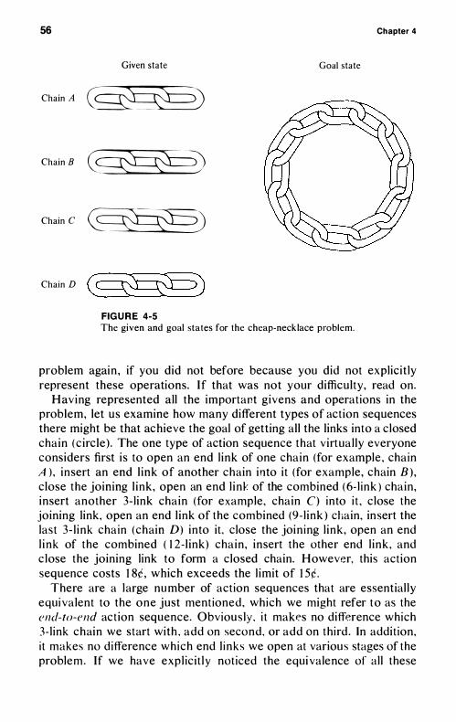
56 Chapter 4

Given state Goal state

Chain A C�)

Chain B C�)

Chain e �)

Chain D

FIG U R E 4-5

The given and goal states for the cheap-neck lace problem.

problem again , if you did not before because you did not explicit ly represent these operations. I f that was not your difficulty, read on.

Having represented all the important givens and operations in the problem, let us examine how many different types of action sequences there might be that achieve the goal of getting all the links into a c losed chain ( c ircle) . The one type of action sequence that virtua l ly everyone considers first i s to open an end l ink of one chain (for example , chain A ) , insert an end l ink of another chain into it (for example, chain B ) , close the joining l ink , open an end l ink of the combined ( 6- l ink ) chain, insert another 3- l ink chain (for example, chain C) into i t , c lose the joining l ink, open an end l ink of the combined (9- l ink ) chain, in sert the last 3 - l ink chain (chain D) into it, close the join ing l ink , open an end l ink of the combined ( 1 2- l ink) chain , insert the other end l ink , and c lose the joining link to form a closed chain. However, this action sequence costs 1 8i , which exceeds the l imit of 1 5i .

There are a l arge number of action sequences that are essential ly equ i valent to the one just mentioned, which we might refer to as the (,lld-to-(,l1d action sequence. Obvious ly , i t mak("s no difference which 3- l ink chain we start with , add on second, or add on th ird . In addit ion, i t makes no difference wh ich end l i nks we open at variou s stages of the problem. If we have expl icit l y noticed the equi valence of al l these

Classification of Action Sequences 57

different action sequences, we are in a favorable position to discover whether there are any action sequences that are not equivalent to end-to-end that might result in the solution. I f you have so far not solved the problem, stop reading and try again .

I t might occur to you that , after opening a l ink, you could insert two end l inks into it or insert a middle l ink. These actions as a part of any action sequence (which did not later essential ly reverse the effect of these actions) would undeniably result in an outcome that was not equivalent to end-to-end. However, a l i ttle inspection of the nature of the goal to be achieved reveal s that, in the final closed chain, there are no l inks that have more than two l inks inserted in them. Thus, all methods that insert two end l inks (of chains with two or more l inks) or a middle l ink (of a chain with three or more l inks) into an end l ink of any chain with two or more l inks could not produce the goal state . (This statement is true unless the critical action were later reversed, and reversing actions seems very un l ikely to be a part of the correct solution, in view of the cost l imitation . )

Assuming that we have heuristical l y rejected a l l action sequences that involve actions that result in three or more links being inserted inside another l ink, are there any other types of action sequences that are not essential l y equivalent to end-to-end? If you have not yet solved the problem, stop reading and try again , then read on.

Yes, there i s exactly one other type, and it i s the solution to the problem. For some reason, this type of action sequence does not occur to many people very quickly, but if you have ru led out al l examples of the previously mentioned two equivalence classes of action sequences, then you are in a rather favorable position for d iscovering this remain­ing type of action sequence. At least, you are not wasting time trying out many specific examples of each of the two large classes of action sequences that do not work.

Perhaps you have al ready di scovered this remaining type of action sequence and perhaps you have not. In any event, this type of action sequence could be called destroying a chain . The action sequence i s as fol lows : Open a l ink of one ( 3 - l ink) chain (for example, chain A ), detach the link from that chain (chain A ) , insert the link into ends of two different 3- l ink chains (for example, B and C) , close the joining l ink ; open another l ink of the chain one is destroying (chain A ) , insert that l ink into an end of the combined (7- l ink) chain and an end of the re­maining 3 - l ink chain (D ) , close the joining l ink ; open the last l ink of the first chain (A ) , insert the ends of the combined ( I I - l ink) chain into it, and close the joining l ink . The cost of this type of action sequence is exactly 1 5i , solv ing the problem within the cost l imitation.

Chapter 4

MACROACTIONS

Now consider a sequence of actions that starts with some given state and achieves some other state . Call that a micro{lctioll sequence. Fur­thermore , consider any other sequence of microactions that starts from the same given state and achieves the same terminal state to be a member of an equivalence class of microaction sequences. Call such an equivalence class a maeroaetion. Thus , a macroaction is defined to be an equivalence class of sequences of microactions, though in some cases the equivalence class may consist of only one member.

Defining one or more macroactions based on the microactions speci­fied in the problem is sometimes a significant aid in solution. If you l ike s i l ly analogies, it is l ike wearing seven-league boots and taking giant steps instead of baby steps. Often, when one has defined macro­actions, the number of such macroactions necessary to go from the givens to the goal is extremely smal l . This means a small state-action tree, with only a relatively small number of distinct possible macro­action sequences to test. Systematic trial and error will often be quite adequate to solve the problem from this point on.

Defining macroactions from sequences of microactions does have one possible d ifficulty, namely, that application of a macroaction might take one past the goal . I n problems with destructive operations, one would have sped past the goal much as an express subway train speeds past a local subway stop. You would not even have the op­portunity to see the goal for an instant as you passed through it, whereas at least on the express subway there is some chance that you could see your local stop as you sped through it .

Even with nondestructive operations, the effect of applying a macroaction that took you past the goal could be much the same as with destructive operations . To be sure, even when you have gone past the goal , you still have ach ieved it in some sense, when the problem involves nondestructive operat ions. However, if you do not know that the goal was achieved, because you never wrote down the goal expression, then in a practical sense , you have not achieved the goal .

As an example of the successfu l use of macroactions and classi­ficatory trial and error, consider the set of possible action sequences involved in reducing an equation of the form ax + b = ex + d to an equa-tion of the form x = ___ . There are a number of different micro-actions in different orders that wil l serve to reduce th is equation. One

Classification of Action Seq uences 59

could subtract b from both sides, then subtract ex from both sides, and then divide both sides by (a - e) , but one could also add -ex to both sides, then multiply both sides by I /(a - e) , and then subtract b/(a - e) from both sides, and so on. To someone experienced in solv­ing such simple algebra problems, this problem may seem pretty trivial , but many students learning elementary algebra for the first time find these problems difficult . One reason for this difference i s that the ex­perienced l inear-equation reducer sees al l these different action se­quences as equi valent, whi le many of the inexperienced l inear-equation reducers have yet to learn this fact . Although probably few people actual ly think in terms of a single equation for l inear-equation reduc­tion, what an experienced l inear-equation reducer has in h is head i s essentially equivalent to a single macroaction for problems of the above type, namely, ax + b = ex + d -+ x = (d - b)/(a - e) . The ex­perienced l inear-equation reducer probably goes through a short se­quence of microactions to solve such a problem, but such a person does this in one of a very small number of completely routinized ways , with, at most , a single choice of one of the equivalent microaction sequences. This statement i s what i s meant by thinking in terms of a single macro­action rather than a sequence of microactions.

Another example of the u sefulness of thinking in terms of macro­actions occurs in geometry construction problems. I n such problems, you are allowed to use a compass , an unmarked straightedge (no grada­tions as on a ruler), and , of course, pencil and paper. The microactions that you have available are then to draw arcs of circles and straight­l ine segments . In learning how to solve geometry construction prob­lems, you first learn what sequences of microactions al low you to achieve certain states , such as construct ing a perpendicular to a l ine at a given point , constructing a perpendicular bisector of a l ine seg­ment, constructing an angle bisector, or construct ing a paral lel to a given l ine through a given outside point. Thereafter, in more complex geometry construction problems, you think in terms of what sequence of these macroactions is necessary in order to solve these geometry construction problems rather than in terms of the original microactions of drawing arcs and circles and straight- l ine segments, though you must use a sequence of such microactions in achiev ing each macroaction. However, in constructing the basic plan for solv ing a more complex geometry construct ion problem, the use of a macroaction i s extremely helpfu l . As an example of how th inking in terms of such macroact ions s impl ifies geometry constru ct ion problems, consider the fo l lowing problem, which was previously discussed briefly in Chapter 3 .

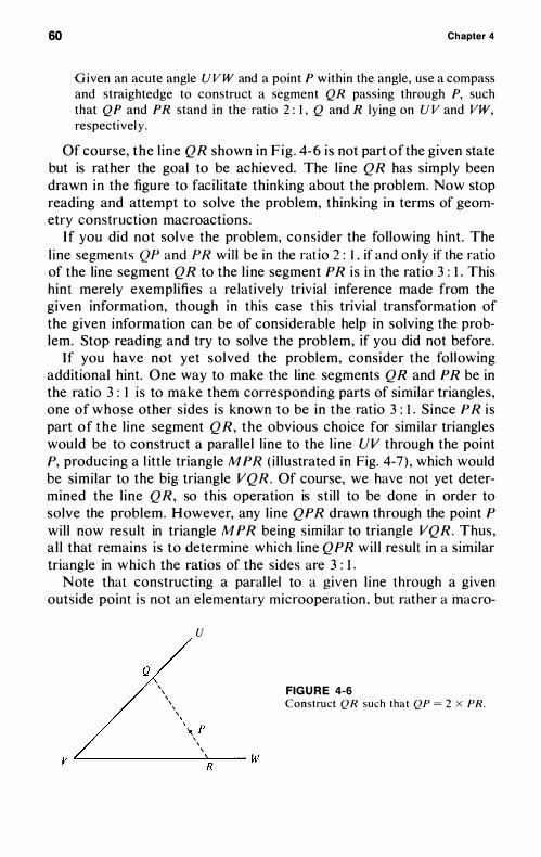
60 Chapter 4

G iven an acute angle U V W and a point P within the angle, use a compass and straightedge to construct a segment QR passing through P, such that QP and PR stand in the ratio 2 : 1 , Q and R lying on U V and VW, respectivel y .

Of course, the l ine QR shown in Fig . 4-6 i s not part of the given state but is rather the goal to be achieved. The l ine QR has simply been drawn in the figure to faci l i tate thinking about the problem. Now stop reading and attempt to solve the problem, thinking in terms of geom­etry construction macroactions.

I f you did not solve the problem, consider the following hint. The l ine segments QP and PR wi l l be in the rat io 2 : L if and only if the ratio of the line segment QR to the l ine segment PR is in the ratio 3 : I . This hint merely exemplifies a relatively triv ial inference made from the given information, though in this case this trivial transformation of the given information can be of considerable help in solving the prob­lem. Stop reading and try to solve the problem, if you did not before.

I f you have not yet solved the problem, consider the following additional hint. One way to make the line segments QR and PR be in the ratio 3 : 1 i s to make them corresponding parts of similar triangles , one of whose other sides i s known to be in the ratio 3 : 1 . Since PR is part of the l ine segment QR, the obvious choice for similar triangles would be to construct a paral lel l ine to the l ine UV through the point P, producing a l ittle triangle MPR (i l lustrated in Fig. 4-7) , which would be similar to the big triangle VQR. Of course, we have not yet deter­mined the l ine QR, so this operation is stil l to be done in order to solve the problem. However, any l ine QPR drawn through the point P wil l now result in triangle MPR being similar to triangle VQR. Thus, a l l that remains i s to determine which l ine QPR wi l l result in a similar triangle in which the ratios of the sides are 3 : I .

Note that constructing a paral lel to a given l ine through a given outside point i s not an elementary microoperation , but rather a macro-

\ , \ \ \ ,

u

\ .. p \ \ , v L..-------->..-- w

R

FIG U R E 4-6 Construct QR such that QP = 2 x PRo

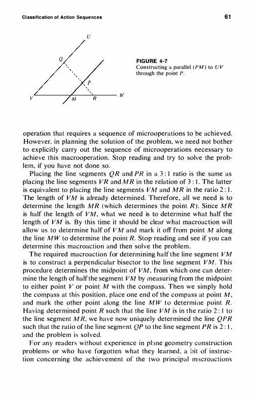
Classification of Action Sequences

u

vL--------,L---��---- W

FIGURE 4-7 Constructing a paral lel ( PM ) to U V through the point P .

61

operation that requires a sequence of microoperations to be achieved. However, in planning the solution of the problem, we need not bother to explicit ly carry out the sequence of microoperations necessary to achieve th is macrooperation . Stop reading and try to solve the prob­lem, if you have not done so.

P lacing the l ine segments QR and PR in a 3 : I ratio i s the same as placing the l ine segments V R and M R in the relation of 3 : 1 . The latter is equivalent to placing the l ine segments V M and M R in the rat io 2 : 1 . The length of VM is already determined. Therefore , al l we need is to determine the length MR ( which determines the point R ) . Since MR is half the length of VM, what we need is to determine what half the length of VM is. By th is time it should be clear what macroaction wi l l a l low us to determine half of VM and mark it off from point M along the l ine M W to determine the point R. Stop reading and see if you can determine th is macroaction and then solve the problem.

The required macroaction for determining ha lf the l ine segment V M is to construct a perpendicular bi sector to the l ine segment VM. This procedure determines the midpoint of VM, from which one can deter­mine the length of half the segment VM by measuri ng from the midpoint to either point V or point M with the compass. Then we simply hold the compass at th is position , p lace one end of the compass at point M , and mark the other point along the l ine M W t o determi ne point R . Having determined point R such that the l ine VM is in t h e rat io 2 : 1 to the l ine segment M R, we have now un iquely determined the line QPR such that the ratio of the l i ne segment QP to the l ine segment PR i s 2 : 1 , and the problem i s solved.

For any readers wi thout experience in pl ane geometry construction problems or who have forgotten what they learned , a bit of instruc­tion concerning the ach ievement of the two principal macroact ions

62 Chapter 4

used in this problem may be he lpful in making the solution of the problem complete ly concrete.

To construct a paral le l to the line UV through the point P, use the arbitrari l y drawn line QPR in Fig. 4- 6 . P lace one point of the compass at point Q and draw an arc through the l ines Q U and QP. The arc may be of any reasonable radius . Now draw an arc of the same radius around the point P. Now use the compass to measure the di stance between intersections of the arc around Q that intersects Q U and QP. To do this operation , place one point of the compass at the inter­section of this arc with the l ine Q U. Now, keeping the same radius with the compass , p lace one point of the compass at the intersection of the arc around the point P with the l ine PR and measure off the same distance along that arc . This point when connected to point P wi l l produce a l ine paral le l to the l ine VQ U.

To achieve the macroaction of bisecting l ine segment VM, place the compass at point V and draw an arc around V intersecting the l ine VM at a point more than halfway between V and M. Now draw the same radius arc around the point M, intersecting the l ine VM and intersecting the arc around V once above the l ine and once below the l ine . Connecting the two intersecting points for the arc around V and the arc around M results in a perpendicular bisector to the l ine VM and therefore determines the midpoint of l ine VM.

Considering how complex especia l ly the first of these two macro­actions i s , in terms of the sequence of required microactions, it is c lear why it fac i l i tates planning the solution of the problem to think in terms of macroactions rather than the sequences of microactions necessary to achieve them.

Knowing wh ich sequences of microactions or equivalence classes of sequences of microactions to define as macroactions appears to depend very heavi ly ( if not completely) on spec ific knowledge of the area from which the problem is taken. General problem-solving analysis makes it c lear what the potential value is in defining macroactions , but i t does not te l l you which macroactions to define in any given prob­lem area. This characteristic is very frequentl y the nature of the rela­tionsh ip between general problem-sol v ing methods and specific knowledge - that is, general problem-sol v ing methods d i rect you toward the type of specific knowledge that you should acqu i re and motivate you to acqu ire this knowledge by demonstrat ing their useful ness in the solu tion of problems .

I ncidental l y, there are other ways to so lve th i s problem, us ing other geometric macroact ions . So, if you thought of a different way to solve the problem, i t may wel l be correct .

63

GETTING OUT OF LOOPS

Beginning problem solvers frequent ly run out of ideas to apply to a problem. H igh ly sk i l led problem solvers often experience the opposite difficu lty ; they have too many ideas and are forced to choose among a variety of possible approaches to the problem. I have devoted some space in th is book to this question of decid ing among many possible problem-solv ing methods , but I have been main ly concerned with the matter of provid ing the student with a rich variety of general methods for attacking problems to ensure that you do not spend a great deal of time staring at a problem without gett ing any ideas.

Sometimes you may have no ideas at a l l as to how to solve a prob­lem, but more frequently you wi l l run out of new ideas after having tried various methods , none of which worked. I n such cases , you may repeatedly think of the inadequate methods for solv ing the problem and get the feel ing that you are going around in circ les . When you are caught in a loop l i ke th is , it is obvious ly time to do something different from what you have been doing. But how? In many cases that seems to be just the trouble : you are in a series of loops, th inking of the same inadequate ideas over and over again .

An excel lent first step in getting out of a loop and doing something different i s to analyze what you have been doing. You must determine the attributes ( properties) of the approaches you have been taking. U sual ly when you make an effort to characterize what you have been doing in try ing to solve a problem, you can immediate ly th ink of some ways to approach the problem differently. Often , what is crit ical is to step back and th ink about what you have been doing rather than think about the problem itself.

There are two basic levels at which th i s analys is of your problem­solv ing methods can take place : ( a) the level of the specific action or action sequences specified in the problem (c lassifying action sequences) and (b ) the level of general problem-solving methods (c lassifying prob­lem-solving methods ) . I n each case, after you have characterized what actions or methods you have used, you should ask what other classes of actions or methods seem remote ly appl icable to the problem.

At the level of general problem-solv ing methods , there are general l y many specific ways to implement any given general method in any part icular problem. What are the propert ies of the way you have chosen? Could you construct an alternat ive way that had different propert ies? Is there any information that i s expl ic i t ly or impl ic i t ly a part of the problem that has not been expl icitly represented? What

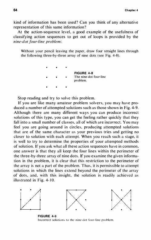
64 Chapter 4

kind of information has been used? Can you think of any alternative representation of this same information?

At the action-sequence level , a good example of the usefu lness of c lassifying action sequences to get out of loops is provided by the nine-dot four-line problem :

Without your pencil leaving the paper, draw four straight l ines through the following three-by-three array of nine dots (see Fig. 4-8).

FIG U R E 4-8 The nine-dot four-l ine problem.

Stop reading and try to sol ve this problem. If you are l ike many amateur problem solvers, you may have pro­

duced a number of attempted solu tions such as those shown in Fig. 4-9 . Although there are many different ways you can produce incorrect solu t ions of this type, you can get the feel ing rather quickly that they fal l into a smal l number of classes, al l of which are incorrect. You may feel you are going around in circ les , producing attempted solutions that are of the same character as your previou s tries and getting no c loser to solution with each attempt . When you reach such a stage, it i s well to try to determine the properties of your attempted methods of sol ut ion. If you ask what al l these action sequences have in common , one answer is that they al l keep the four l ines with in the perimeter of the three-by-three array of nine dots. If you examine the given informa­tion in the problem, it is c lear that th is restriction to the perimeter of the array is not a part of the problem. Thus , it is permiss ible to attempt solu t ions in which the l ines extend beyond the perimeter of the array of dots , and , with this insight , the solut ion is read i ly achieved as i l lu strated in Fig. 4- \ O.

FIG U R E 4-9 I ncorrect sol u t i o n , t o the n i ne-dot fou r- l i n e p robl e m .

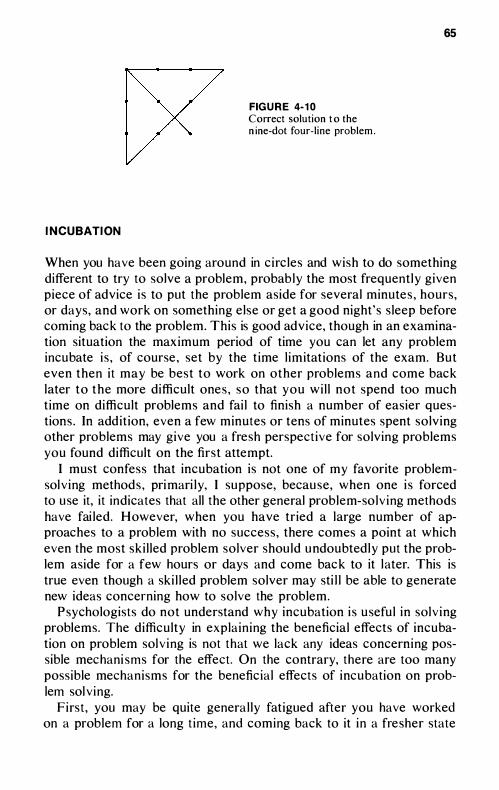
INCUBATION

FIG U R E 4- 1 0 Correct solution t o the n ine-dot four-line problem .

65

When you have been going around in circ les and wish to do something different to try to solve a problem, probably the most frequently given piece of advice is to put the problem aside for several minutes , hours, or days, and work on something else or get a good night' s sleep before coming back to the problem. This is good advice, though in an examina­tion situation the maximum period of time you can let any problem incubate is , of course , set by the time l imitations of the exam. But even then it may be best to work on other problems and come back later to the more difficult ones , so that you wi l l not spend too much time on difficult problems and fai l to finish a number of easier ques­tions . In addition, even a few minutes or tens of minutes spent solving other problems may give you a fresh perspective for solving problems you found difficult on the first attempt.

I must confess that incubation is not one of my favorite problem­solving methods , primari ly, I suppose, because, when one i s forced to use it, it indicates that all the other general problem-solv ing methods have fai led. However, when you have tried a large number of ap­proaches to a problem with no success, there comes a point at which even the most ski l led problem solver shou ld undoubtedly put the prob­lem aside for a few hours or days and come back to it l ater. This is true even though a ski l led problem solver may sti l l be able to generate new ideas concerning how to solve the problem.

Psychologists do not understand why incubation i s useful in solv ing problems. The difficulty in explaining the beneficial effects of incuba­tion on problem solv ing is not that we lack any ideas concerning pos­sible mechani sms for the effect. On the contrary, there are too many possible mechanisms for the beneficial effects of incubation on prob­lem sol ving.

First , you may be quite general ly fatigued after you have worked on a problem for a long t ime, and coming back to it in a fresher state

66 Chapter 4

of mind seems l ike ly to be beneficial (though again we do not under­stand the mechanisms of general inte l lectual fatigue or the need for sleep and so on) .

Second , there may be more specific intel lectual fatigue or inter­ference in the use of your memory because of the large number of incorrect actions you have taken in trying to solve the problem. The passage of t ime filled with intervening activit ies provides an oppor­tunity for these interfering memories to fade away. Only the most valuable lessons you have learned remain in the foreground of your mind when you go back to the problem, with a host of lesser interfering associations having decayed to a low level . It is not c lear that this sort of memory loss should necessari ly be beneficial to problem solv­ing, but it wel l might be.

Third , when you come back to the problem, you have an altered memory and new set of things on your mind as a result of the inter­vening act iv ity. These new associations and new cues may wel l result in the retrieval of new ideas from memory concerning how to solve the given problem. This explanation i s probably the s ingle most plaus ib le reason for the success of the method of incubation.

There i s a fourth , somewhat more exotic possibi l ity, namely, that a person' s mind goes on unconscious ly working the problem all during the long incubation period . Either because the unconscious mind has a long time to work on the problem or because someth ing special i s added by unconscious problem solving, the problem manages to get solved in this way, when conscious problem solv ing has fai led. I n any event, the unconscious problem solv ing may modify memory in a man­ner that faci l i tates conscious problem solv ing at a later time. There i s not one shred of evidence for thi s explanation of incubation, whereas the first three possible mechan isms are all extensions of previou s ly establ i shed psychological principles . N evertheless , many psycholo­gi sts bel ieve in unconsc ious problem solv ing. I am very skeptical on the matter, but that i s primari l y a matter of ph i losophical preference.

In any event, incubation often works, whatever the mechan ism.

THEORY

5

State Evaluation

and Hill Climbing

In the last chapter we reduced the amount of trial-and-error search in a problem by constructing equivalent state-action trees of reduced size. In this chapter, we d iscuss a very different way of reducing the number of state-action sequences that have to be searched before achieving the solut ion. The method has two parts : (a) defining an evaluation jimclion over all states inc luding the goal state and (b ) choos­ing actions at any given state to achieve a next state with an evaluation closer to that of the goal . P icking an action on the basis of such a local evaluation of i ts consequences i s known as hill climbing, s ince evaluation functions are frequent ly defined so that the goal state has the maximum value on some one-d imensional evaluation function.

Figure 5. 1 i l l u strates the appl ication of state evaluation and h i l l c l imbing to the state-action tree for some unknown problem wi th a hypothetical evaluation function defined over each state. The value of the function for each state is written inside the c i rc le for each node ( state) . This example arbitrari l y u ses an i nteger-valued evaluation function, with the begi nning state hav ing value 0 , the goal state having value 1 0 , and nongoal states having values intermediate between °

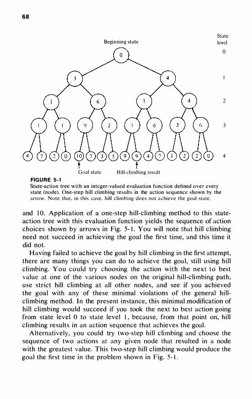
68

Begin ning state State

leve l

Goal state Hil l-cl imbing result

FIG U R E 5-1

State-action tree with an integer-valued evaluation function defined over every state (node). One-step hi l l c l imbing results in the action sequence shown by the arro w . N ote that, i n t h i s case, h i l l c l i m b i ng does not achieve the goal state .

o

2

3

4

and 1 0 . Application of a one-step hi l I-c l imbing method to this state­action tree with this evaluation function yields the sequence of action choices shown by arrows in Fig. 5- 1 . You wiII note that hi l I c l imbing need not succeed in achieving the goal the first time, and this time it did not.

H aving fai led to achieve the goal by h i l l c l imbing in the first attempt, there are many things you can do to achieve the goal , sti l l u sing h i l l c l imbing. You cou ld try choosing the action wi th the next to best value at one of the variou s nodes on the original h i l l-c l imbing path, use strict hil l c l imbing at all other nodes, and see if you achieved the goal with any of these minimal violations of the general h i l l­c l imbing method . I n the present instance, this minimal .modification of h i l l c l imbing would succeed if you took the next to best action going from state level 0 to state level l , because, from that point on, h i l l c l imbing results in an action sequence that ach ieves the goal .

A lternative ly, you could try two-step h i l l c l imbing and choose the sequence of two actions at any given node that resul ted in a node with the greatest value . This two-step h i l l c l imbing would produce the goal the first t ime in the problem shown in Fig. 5 - 1 .

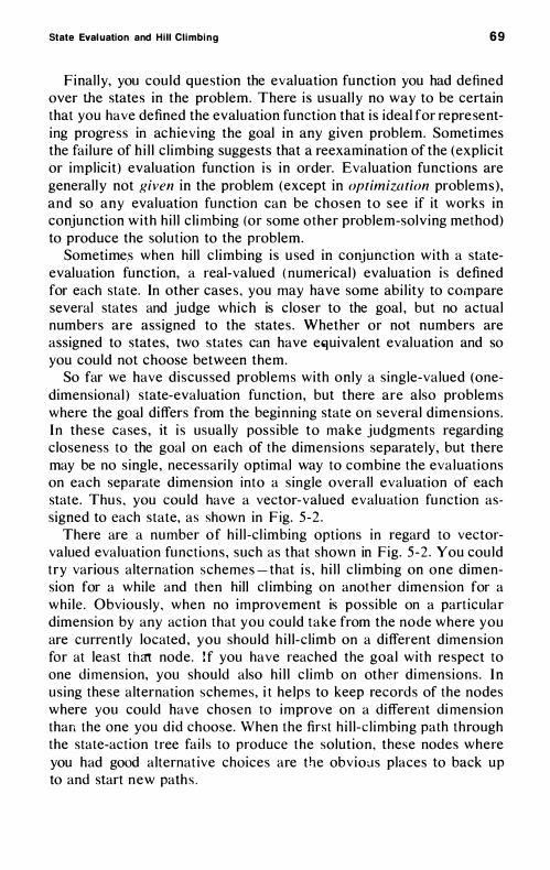
State Evaluation and Hill Climbin g 69

Final ly, you cou ld question the evaluation function you had defined over the states in the problem. There i s usual l y no way to be certain that you have defined the evaluation function that i s ideal for represent­ing progress in achieving the goal in any given problem. Sometimes the fai lure of h i l l c l imbing suggests that a reexamination of the (expl icit or impl icit) evaluation function is in order. Evaluation functions are general ly not given in the problem (except in optimization problems) , and so any evaluation function can be chosen to see if it works in conjunction with h i l l c l i mbing (or some other problem-solving method) to produce the solu tion to the problem.

Sometime.s when hi l l c l imbing i s used in conjunction with a state­evaluation function, a real-valued ( numerical ) evaluation is defined for each state. In other cases , you may have some abi l ity to compare several states and judge which is closer to the goal , but no actual numbers are assigned to the states . Whether or not numbers are assigned to states, two states can have e'luivalent evaluation and so you cou ld not choose between them.

So far we have discussed problems with only a single-valued (one­dimensional ) state-evaluation function, but there are also problems where the goal differs from the beginning state on several dimensions. I n these cases , it i s usual ly possible to make judgments regarding closeness to the goal on each of the dimensions separately, but there may be no s ingle , necessari ly optimal way to combine the evaluations on each separate dimension into a single overal l evaluation of each state. Thus , you cou ld have a vector-valued evaluat ion function as­signed to each state, as shown in F ig. 5-2 .

There are a number of h i l l -cl imbing options in regard to vector­valued evaluation functions , such as that shown in Fig. 5-2 . You cou ld try variou s alternation schemes - that i s , h i l l c l imbing on one dimen­sion for a while and then hi l l cl imbing on another dimension for a whi le . Obviously, when no improvement is possible on a part icular dimension by any action that you could take from the node where you are current ly located , you shou ld h i l l -c l imb on a different dimension for at least that node. I f you have reached the goal with respect to one dimension, you should also h i l l c l imb on other dimensions. I n using these alternation schemes, i t he lps to keep records of the nodes where you cou ld have chosen to improve on a different di mension than the one you d id choose. When the first h i l l-c l imbing path through the state-action tree fai l s to produce the solution , these nodes where you had good alternat ive choices are the obvious places to back up to and start new path s .

70

Beginning state State level

o

2

3

Goa l state FIG U R E 5-2 State-action tree with a two-dimensional vector-valued evaluation function defined over every state (node) . In this case. the goal state has the evaluation vector ( 5 . 4), and the beginning state has the evaluation vector (0, 0) . The path taken by a hi l l c l im bing method depends o n whether you h i l l c l imb on weighted s u m m e d components o r try some al ternation s c h e m e . In t h e fo rmer case. the exact weigh ing of t h e two c o m p o n e n t va lues i s a l so i m portant i n determ i n i n g the path taken by h i l l c l i mb i ng .

Another approach to mult id imensional evaluation functions i s to combine the values on the separate d imensions i nto a s ingle overal l value for each state . If there i s some s ingle most natural way to com­bine them . do i t that way first ; but remember that . no matter how natural the combination method might be, it could be the wrong way to combine the values on the different dimensions - that i s , wrong for achiev ing the solution by one-dimensional h i l l c l imbing. If the orig­inal l y chosen combination method fai l s to work , try some other method of combination, alternation schemes with the original mult id imensional evaluation function , mul t i step h i l l c l imbing, defining a new evaluation funct ion, or the l i ke .

APPLICATIONS

Examples of the u se of state-eval uation functions and h i l l c l imbing abound i n problem solv ing. For instance, when you plan a tr ip across the country on a map. you in i t ia l ly examine roads that go in nearly the right d i rection. The right d i rection is the d i rection that reduces the d i stance between where you are and where you are going at the fastest rate . Of cou rse, choos ing the road at the beginning of a tr ip that goes c losest to the right d i rect ion may prove to be a bad choice .

State Eval uation and Hil l Climbing 71

This road may eventual l y lead to a dead end or require you to go far out of the way to reach the goal . I n addition , planning a trip on a map usual ly involves other considerations - speed , scenery, or other properties - besides finding the shortest road between the starting and ending points. These considerations place you in the position of doing h i l l c l imbing on a vector-valued evaluation function. Despite al l these complications, experience suggests that h i l l c l imbing is a prominent method used in solving trip planning problems with a map.

Pencil-and-paper maze problems are rather similar to trip-planning problems on a map, and people frequently use hil l c l imbing in an at­tempt to solve them. However, chal lenging maze problems are u sua l ly del iberately constructed to frustrate a h :n-c 1 imbing approach. Maze problems frequently requ ire nonoptimal choices at early and middle stages of the solution and may even require detours ( increases in the di stance from the goa l , as measured by the most obvious evaluation function of physical di stance) . On the other hand , maze problems usual l y do not involve considerations of road speed or scenic beauty.

Defining an explicit evaluation function and employing h i l l c l imbing is also usefu l in solv ing the one-heavy-coin problem discussed in Chapter 3 :

You have a pile of 24 coins. Twenty-three of these coins have the same weight, and one i s heavier. Your task is to determine which coin i s heavier and to do so in the minimum number of weighings . You are given a beam balance ( scale ) , which will compare the weight of any two sets of coins out of the total set of 24 coins .

A su itable evaluation function for solv ing th is problem would be the number of coins whose c lassification as heavy or l ight is known. At the beginning of the problem, the value of the function is zero , since none of the 24 coins is known to be either heavy or l ight. In the goal state , the heavy-light c lassification of a l l 24 coins i s known , so the value of the function is 24 . Thus, a h i l l -c l imbing approach wou ld choose an action at each node that maximized the number of coins whose heavy­l ight classification is known.

A very large number of alternative actions are present at each node. For example , at the first node, you might weigh any one of the coins against any two of the other coins. I n general , you might weigh any set of m coins against any set of n coins, where n + m :5 24 . The num­ber of different pairs of sets of m and n coins that sati sfy the restriction that m + II :5 24 is extremely large . However, the most elementary considerat ion of the previous ly mentioned evaluation function and

72 Chapter 5

the hi l l -c l imbing approach immediate ly rules out al l actions that do not involve weighing two sets containing equal numbers of coins in the two pans of the beam balance. This exclusion reduces the number of alternative actions considerably.

Furthermore , using the method of defining equivalence c lasses of actions discussed in Chapter 4 , note that, at the first node of the problem, you have no way to distinguish different subsets of i coins ; thus , you must consider any two sets of i coins to be equivalent to each other ( in their l ike l ihood of containing the heavy coin) . This con­sideration reduces the number of different alternative actions at the first node to 1 2 - that i s , a set of 1 2 coins is weighed against a set of 1 2 coins, a set of 1 1 coins against another set of 1 1 coins , 1 0 against 1 0 , and so on, or 1 against 1 .

I f you expl icit ly inquire which of these 1 2 alternative actions results in the greatest number of known coins fol lowing the first weighing, you should be led to select the optimal action at the first node - that is , to weigh a set of 8 coins against another set of 8 coins , s ince this maximal ly increases the value of the evaluation function from 0 known coins to 1 6 known coins fol lowing the first weighing, whatever the out­come of the first weighing.

The same sort of evaluation function and h i l l -c l imbing approach can be used to solve more complex coin-weigh ing problems, such as those involving two heavy coins or one coin that might be either heavier or l ighter than the other coins . When the coins are c lassified into three or more categories (for example , heavy, medium, and l ight) , then it may be usefu l to u se as an evaluation function the number of coin-classification pairings (for example , coin I is heavy, coin 2 is medium, coin 3 i s l ight) that have been ruled out .

In a l l of the coin-weighing problems, from the simplest to the most complex , keep in mind that, after a given weighing, the value of the evaluation function may be different for the different outcomes of the weighing. In such cases , the value of the evaluation function for a particular weigh ing is usua l ly best considered to be the expected value of the evaluation function across al l different outcomes, where the value of the evaluation function for each outcome is weighted by the probabi l i ty of obtaining that outcome. Thus , after the first weigh­ing of eight coins against eight coins in the previous ly mentioned one-heavy-coin prob lem, the optimal choice in the second weighing is either to weigh two coins against two coins or three coins against three coins . In either case, the three outcomes of the weighing ( t i l t left , bal­ance, tilt right) are not equal l y l i kely, nor does each outcome resu l t in an equivalent increase in the number of known co ins . For example , wi th

State Eval uation and Hill Climbing 73

the three against three weighing (out of the eight remaining coins) , the probabil ity of their balancing evenly i s � , while the probabi l i ty of tilt left is � , and the probabi l ity of ti l t right i s � .

For simpl icity, let u s u se as the evaluation function the nu mber of unknoll 'll coins, where the goal state has a value of zero unknown coins . Thus , h i l l c l imbing, in th is case, means attempting to minimize the value of the evaluation function. U s ing this evaluation function, the value of a balanced outcome in the three-against-three weighing is two remaining unknown coi ns , whi le the value of t i l t left is 3 and the value of t i l t right is also 3 . The overal l evaluation of the three-against­three weigh ing, then, is (� . 3) + (� . 3) + (� . 2) = ¥ = 21 .

The three-against-three weighing produces the minimum expected value on the evaluation function. This fact can be seen by computing the expected value for the other three plausible weighings - namely , one against one, two against two, and four against four. The two­against-two weighing is almost as good as the three-against-three weighing, by this evaluation function. The two-against-two weighing has an expected value of (i ' 2) + (i . 2) + (4 ' 4) = 3. The four-against­four weighing has an expected value of a . 4) + (4 . 4) = 4. The one­against-one weighing has the poorest expected value of al l - namely, (� . 0) + (� . 0) + (* . 6) = 44 .

I n terms of achiev ing the goal of determining the one heavy coin out of 24 in the minimum number of weighings, either the three-against­three weighing or the two-against-two weighing i s optimal on the second weighing. Thus , in this case , hi l l c l imbing i s a successfu l prob­lem-solv ing method , since it chooses one of the two actions that wi l l lead to the goal wi th the min imum nu mber of total actions (weighings) .

Sol v ing s imple l inear equations provides another example of the possibi l i ty of successfu l use of h i l l c l imbing in problem solv ing. Con­sider the l inear equation 9x + 7 = 5x + 15 as the given, with an expres-sion of the form x = ___ being the goal . The blank, ___ , repre-sents some currently unknown real number that constitutes the value of x in the solution to the equation.

I n it ial l y, we might define a four-valued vector eval uation function for this problem, consist ing of the coefficients of the x and nu merical terms on the left-hand side of the equation and the x and numerical terms on the right-hand side. For the l inear equation above, then, the value of the evaluation function at the given state wou ld be (9 , 7, 5 , 1 5 ) . The value of the evaluation fu nction for the goal state i s ( 1 , 0, 0 , ___ ) , where ___ again ind icates that we do not current ly know what real nu mber is acceptable in th is posit ion. We might choose actions at each step designed to increase the number of terms of th i s

74 Chapter 5

four-valued vector evaluation function that are in agreement with the corresponding terms of the evaluation function for the goal . Thus , if we subtract 5x from both sides of the equation , the evaluation function is changed to (4 , 7, 0, 1 5 ) , which is known to di sagree with the evaluation function for the goal in only the first two positions (the agreement of the value in the fourth position with the desired value in the goal expression cannot be determined ) . Subsequent ly, subtracting 7 from both sides of the equation changes the evaluation function to (4 , 0, 0, 8 ) , which disagrees with the goal express ion in only one posi­tion ( the first ) . F inal l y, d iv iding both sides of the equation by 4 has an evaluation function ( 1 , 0 , 0, 2 ) , which is known to disagree with the evaluation function for the goal in zero positions. The state achieved at th i s point that includes the expression x = 2 constitutes the solut ion to the problem.

Rather than th ink of th is at al l in terms of a four-valued vector evaluation function, we can simply th ink of the number of "bad" terms in the expression. I n itial l y there are three bad terms. After subtract ing 5x from both sides of the equation (obtaining 4x + 7 = 1 5) , there are on ly two known bad terms. After subtracting 7 for both sides (obtaining 4x = 8), there is only one known bad term. Final l y, after div id ing both sides of the equation by 4 (obtaining x = 2 ) , there are no bad terms, and the problem is solved.

I t may be somewhat difficul t for someone experienced in solving such s imple l inear equations to imagine that anyone actual l y uses th is sort of evaluation function and h i l l c l imbing in order to solve so s imple a problem. H owever, th is approach cou ld be used, and , very l ike ly, many beginning algebra students unconsiou s ly use just such a method in sol v ing their in itial l inear-equation problems .

The more experienced l inear-equation sol ver very l ike ly th inks of the problem in terms of three subgoal s , namely, getting al l the x terms on the left side of the equation, getting all the numerical terms on the right side of the equation , and div iding through by the coefficient of the x term. However, th i s subgoal method ( to be described in detail in the fol lowing chapter) u ses the same sort of evaluation function as u sed by the h i l l -c l imbing approach to l i near-equation problems.

Once you are an experienced solver of l inear equat ions you probably never think of eval uation functions , subgoal s , or hi l l c l imbing at al l but simply solve the problem us ing the same type of action sequence you have used in sol ving other such p roblems - namely, subtract the x term on the right-hand side of the equation from the x term on the left-hand side of the equation , then subtract the numerical term on the left-hand side of the equation from the numerical term on the

State Evaluation and Hil l Climbing 75

right-hand side of the equation , and final ly divide through by the coefficient of the x term . (This problem-solv ing method , knowing how to solve a problem because you recognize its re lationship to other problems you solved previou s ly, will be discu ssed in Chapter 9 . ) Thus , there are many different problem-solv ing methods that can all lead to roughl y the same sequence of actions in solv ing a simple l inear­equation problem. This s imple problem is discussed primari ly to com­municate what is meant by such concepts as evaluation functions , h i l l c l imbing, subgoal s , re lations between problems , and the l i ke .

Furthermore, h i l l c l imbing i s frequent ly u sed to solve more complex equations or sets of equations , u s ing as an evaluation function some measure or measures of the di screpancy in form between some equa­tion you have produced and the goal equation. Thus , in solv ing equations involving exponential terms with the unknown in the ex­ponent, a solver often takes logs of both sides of the equation to increase the s imi larity of the resu l t ing equation to the goal equation ( since in the goal equation the unknown i s not in the exponent). I n solving differential equations , you can integrate t o get rid of the differential terms, and in sol v ing integral equations , you can solve for the integral s or else differentiate in order to get rid of integral s , and so on.

The six-arrow problem discu ssed in Chapter 4 to i l lustrate the power of noticing equivalence c lasses of action sequences provides a very good example of a problem in which you can define multiple - at least three - different evaluation functions. The three evaluation functions differ considerably in their effectiveness for a hi l l -c l imbing approach . Recal l that the six-arrow problem is as fol lows :

You are given s ix arrows in a row, the left three of which are pointing up and the right three of which are pointing down. The goal i s to transform these arrows into an alternat ing sequence such that the left-most arrow points up, the next arrow to it points down, the next up, then down, then up, and then down. The actions allowed are to s imul taneous ly invert ( turn upside down) any two adjacent arrows. Note that you may not invert one arrow at a time but must invert two arrows at a t ime, and the two must be adjacent. The given and goal states are i l lustrated in Fig. 5-3 . You are to achieve the solution using the min imum number of act ions ( i nversions of adjacent pairs ) .

Stop read ing and try to define three different evaluation functions that might be relevant to solving th is problem by hi l l c l imbing, then read on.

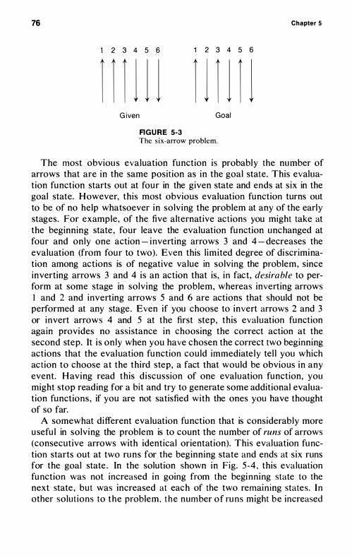
76 Chapter 5

2 3 4 5 6 2 3 4 5 6

r r r 1 1 1 r 1 r 1 r 1 G iven Goal

R G U R E 5-3 The s ix-arrow problem.

The most obviou s evaluation function is probably the number of arrows that are in the same position as in the goal state. This evalua­tion function starts out at four in the given state and ends at six in the goal state. However, this most obvious evaluation function turns out to be of no help whatsoever in solving the problem at any of the early stages. For example , of the five alternative actions you might take at the beginning state , four leave the evaluation function unchanged at four and only one action - inverting arrows 3 and 4 - decreases the evaluation (from four to two). Even this l imited degree of di scrimina­tion among actions is of negative value in solving the problem, since inverting arrows 3 and 4 is an action that is, in fact, desirable to per­form at some stage in solving the problem, whereas inverting arrows I and 2 and inverting arrows 5 and 6 are actions that should not be performed at any stage . Even if you choose to invert arrows 2 and 3 or invert arrows 4 and 5 at the first step, this evaluation function again provides no assistance in choosing the correct action at the second step. It i s only when you have chosen the correct two beginning actions that the evaluation function could immediate ly tel l you which action to choose at the third step, a fact that would be obvious in any event. Having read this d iscussion of one evaluation function, you might stop reading for a bit and try to generate some additional evalua­tion functions , if you are not satisfied with the ones you have thought of so far.

A somewhat different evaluation function that is considerably more usefu l in solving the problem is to count the number of runs of arrows (consecutive arrows with identical orientation). This evaluation func­tion starts out at two runs for the beginning state and ends at six runs for the goal state . In the solution shown in Fig. 5 -4 , this evaluation function was not increased in going from the beginning state to the next state , but was increased at each of the two remain ing states. In other solut ions to the problem, the number of runs might be increased

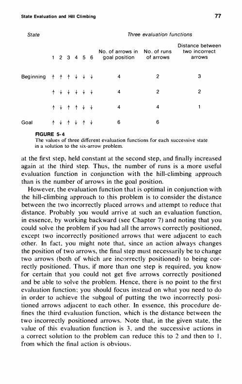
State Evaluation and Hill Cl imbing 77

State Three evalua tion functions

Distance between No. of arrows in No. of run s two incorrect

1 2 3 4 5 6 goal posit ion of arrows arrows

Begi n n i ng t t t t t t 4 2 3

t t t t t t 4 2 2

t t t t t t 4 4

Goal t t t t t t 6 6

RGURE 5- 4 The values of three different evaluation functions for each success ive state in a solution to the s ix-arrow problem.

at the first step, held constant at the second step, and final l y increased again at the third step. Thus , the number of runs i s a more useful evaluation function in conjunction with the hi l l -c l imbing approach than is the number of arrows in the goal position.

However, the evaluation function that i s optimal in conjunction with the h i l l -c l imbing approach to this problem is to consider the distance between the two incorrectly placed arrows and attempt to reduce that distance . Probably you would arrive at such an evaluation function, in essence, by working backward (see Chapter 7) and noting that you could solve the problem if you had al l the arrows correct ly positioned , except two incorrect ly positioned arrows that were adjacent to each other. In fact , you might note that, since an action always changes the position of two arrows, the final step must necessari ly be to change two arrows ( both of which are incorrect ly positioned) to being cor­rect ly positioned . Thus, if more than one step is required , you know for certain that you cou ld not get five arrows correctly positioned and be able to solve the problem. Hence, there is no point to the first evaluation function ; you should focus instead on what you need to do in order to ach ieve the subgoal of putting the two incorrect ly posi­tioned arrows adjacent to each other. In essence, this procedure de­fines the th ird evaluation function, which i s the di stance between the two incorrectly positioned arrows. N ote that , in the given state , the value of this evaluation function is 3 , and the successive actions in a correct solut ion to the problem can reduce th is to 2 and then to I , from which the final action is obviou s .

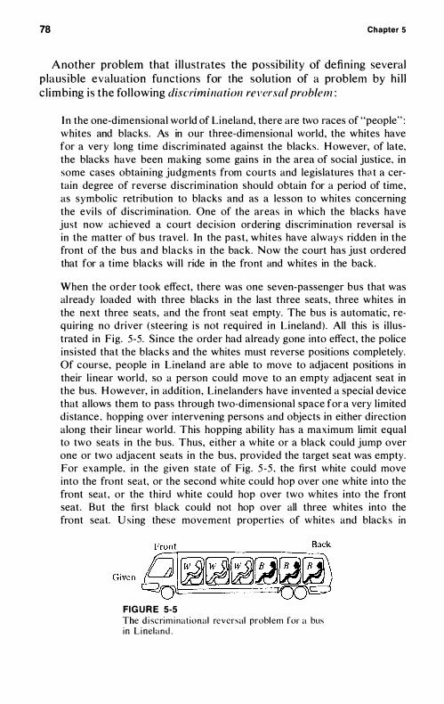
78 Chapter 5

Another problem that i l l ustrates the possibi l ity of defining several p lausible evaluation functions for the solu tion of a problem by h i l l c l imbing is the fol lowing discrimination re l 'ersal problem :

I n the one-d imensional world of Lineland, there are two races of "people" : whites and blacks . As in our three-dimensional world, the whites have for a very long t ime d iscriminated against the blacks . H owever, of late, the blacks have been making some gains in the area of social justice, in some cases obtain ing judgments from courts and legislatures that a cer­tain degree of reverse d i scrimination should obtain for a period of t ime, as symbolic retribution to blacks and as a lesson to whites concerning the evi l s of d iscrimination. One of the areas in which the blacks have just now achieved a court decis ion ordering di scrimination reversal is in the matter of bus travel . In the past , whites have always ridden in the front of the bus and blacks in the back . Now the court has just ordered that for a t ime blacks wi l l ride in the front and whites in the back.

When the order took effect, there was one seven-passenger bus that was al ready loaded with three blacks in the last three seats , three whites in the next three seats, and the front seat empty. The bus is automatic, re­quiring no driver (steering i s not required in Lineland) . All this is i l lus­trated in Fig. 5-5. S ince the order had already gone into effect, the police insi sted that the blacks and the whites must reverse positions completely. Of course, people in Lineland are able to move to adjacent positions in their l inear world , so a person could move to an empty adjacent seat in the bus. H owever, in addit ion, Linelanders have invented a special device that allows them to pass through two-d imensional space for a very l imited d i stance , hopping over intervening persons and objects in either direction along their l inear world . This hopping abi l i ty has a maximum limit equal to two seats in the bus. Thus, either a white or a black could jump over one or two adjacent seats in the bus, provided the target seat was empty. For example, in the given state of Fig. 5 -5 , the first white could move into the front seat, or the second white could hop over one white into the front seat , or the th ird white could hop over two whites into the front seat . But the first black could not hop over all three whites into the front seat. U s ing these movement propert ies of whites and blacks in

FIG U R E 5-5

The d i sc ri m i nat ional re versal probl em for a bus in L i neland .

State Evaluation and Hill Climbing 79

Lineland , solve the problem of reversing the relative posit ions of the blacks and the whites so that all three blacks are in front of al l three whites in the bus . Do this in the min imum number of moves. In solv ing the problem, note that it is i rrelevant to the sati sfaction of the court order where the empty seat occurs in the bus, so long as al l three blacks are sitt ing in front of all three whites.

I t i s not possible in this problem to write down a s ingle goal state , since a variety of possible goal states wi l l satisfy the problem. A l l we can say for sure is that, in the goal state , the first four positions in the bus will contain al l three blacks and the last four seats in the bus wi l l contain al l three whites, but one does not know where the empty seat wil l occur. This l imited specification of the goal state , however, is quite adequate for defining a variety of evaluation functions that ap­pear re levant to the solution of the problem. At this point, stop read ing and , us ing a h i l l -c l imbing approach , try to define expl ic i t ly some evalua­tion functions that might prove useful for sol ving the problem.

There appear to me to be two obvious types of evaluation functions we can define for this problem, both of which are quite satisfactory for hi l l c l imbing. One evaluation function involves numbering the positions in the bus from I at the front to 7 at the back. The evaluation function would be someth ing l ike the average position of the whites minus the average position of the blacks. We cou ld then attempt to maximize th is number. With this evaluation function , a detour i s required on the first move , but thereafter all moves in the optimal sequence do increase this evaluation function by an amount that is either greater than or equal to every other alternative action (usual ly greater than every other alternative action) . Expl icit computation of the value of this function is somewhat more difficult than the second evaluation function to be discu ssed , but al l that real ly counts is the relative difference between the current state and every alternative state that can be achieved by taking any admissible action. This difference is re lative ly easy to determine, and so th is evaluation function proves qu ite help­fu l in conjunction with a hi l l -c l imbing approach to solving the problem. If you have not yet thought of a second evaluation function for the solut ion of this problem, stop reading and try to think of another one.

A second evaluation function , which i s even easier to compute than the first , i s the sum of the number of blacks in front of each white , summed across a l l whites. The value of th i s evaluation function for every state starting with the beginning state and ending with the goal state in the optimal solution of the problem is shown in F ig. 5 - 6 . Clearly,

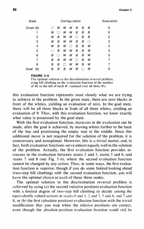
80 Chapter 5

State Configuration Evalua tion

G iven (0) D W W W B B B 0

1 W D W W B B B 0

2 W B W W D B B 2

3 W B W W B B D 2

4 W B W D B B W 4

5 D B W W B B W 5

6 B D W W B B W 5

7 B B W W D B W 7

8 B B D W W B W 7

G oa l (9) B B B W W D W 9

R G U R E 5 - 6 T h e optimal solut ion t o t h e discrimination reversal problem . us ing h i l l c l imbing on the evaluation function of the number of B s to the left of each W. summed over all three Ws.

th is evaluation function represents most closely what we are trying to ach ieve in the problem. In the given state , there are zero blacks in front of the whites , yielding an evaluation of zero. In the goal state, there wil l be all three blacks in front of all three whites , yielding an evaluation of 9. Thus , with this evaluation function , we know exactly what value i s possessed by the goal state .

With the first evaluation function , increases in the evaluation can be made, after the goal is achieved , by moving whites further to the back of the bus and positioning the empty seat in the middle. Since this additional move is not required for the solution of the problem, it is unnecessary and nonoptimal . However, this is a trivial matter, and , in fact, both evaluation functions serve almost equai ly wel l in the solution of the problem. Actual ly , the first evaluation function provides in­creases in the evaluation between states 2 and 3 , states 5 and 6, and states 7 and 8 ( see Fig. 5 - 6) , where the second evaluation function cannot be changed by any action. Thus , in some ways , the first evalua­tion function is superior, though if you do some l imited looking ahead (two-step hi l l c l imbing) with the second evaluation function , you wi l l have the optimal choice at each of these three nodes.

The optimal solution to the discrimination reversal problem is ach if.'ved by us ing (a) the second ( re lative position) evaluation function with a l imi ted degree of two-step h i l l c l imbing to decide among the equ i va lent ly valued act ions in s ta tes 0 and 1 . 2 and 3 . :; and 6. and 7 and 8 , or (b ) the first (absolute pos i t i on ) evaluat ion function wi th the tr ivial modification that you stop when the relative posit ions are correct . even though the absolu te-posit ion evaluation function could s t i i l be

State Evaluation and Hill Climbing 81

increased . It is a remarkable fact concerning the absolute-position evaluation function that it permits choice of the optimal action at each state , using a hil l-cl imbing approach. That is, hill c l imbing using the absolute-position evaluation function will produce the solution the very first time by choosing the action that maximizes the evaluation on the next state (bearing in mind that, at the first move, you must choose the action that reduces the absolute position evaluation by the least amount).

The definition of evaluation functions and the use of hill c l imbing have a substantial role in playing chess games and in the solution of many chess problems. However, there are at least two major difficul­ties in the use of hi l l c l imbing in chess. First, even the immediate evaluation of any move you take must depend to some extent on your opponent 's immediate ly fol lowing move. This fact leads to a certain degree of uncertainty, but it can be resolved in at least two ways : (a) by assigning sUbjective probabilit ies to your opponent ' s different moves and accordingly determining the expected values of your own possible moves (as was done in the "game against nature" i l lustrated by the coin-weighing problem) and (b) by assigning an evaluation to your move consistent with the best next move your opponent could produce (where this move is in any sense determinable) . Since your subjective probabi l ities for your opponent's moves are l ikely to be only approximately accurate at best and since your abil ity to judge your opponent's best response is l imited as wel l , there are substantial diffi­culties in applying hi l l cl imbing, no matter which approach is taken.

The second principal d ifficulty of using hi l l c l imbing in chess con­cerns the very large variety of different evaluation functions that are relevant to playing a good game of chess or solving many chess prob­lems. For example, you are concerned with moving your own pieces to favorable positions on the board (where they control large numbers of squares), the subsidiary goal of control of the center, preventing your opponent' s piece development, ensuring the safety of your king, jeopardizing the safety of your opponent's king, and many, many others. I t is not at all obvious what all the relevant evaluation func­tions might be in chess nor how to weight them in d ifferent situations to come up with some overal l evaluation of your next move .

Despite all these problems, the defining of evaluation functions and the use of hi l l c l imbing ( looking ahead one or more steps) are important problem-solving methods in chess. To i l lustrate , consider the fol lowing very simple end-game problem involving black's rook and king against white 's king, with the positions as i l lustrated in F ig. 5-7 and b lack to move. It is black's move and b lack's objective is to checkmate the

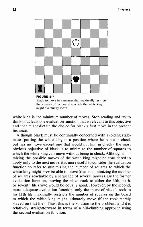
82

,

0 I

-I J

FIGURE 5-7

Black to move in a manner that maximally restricts

the squares of the board to which the white k ing

might eventual ly move.

Chapter 5

white king in the minimum number of moves . Stop reading and try to think of at least one evaluation function that is relevant to this objective and that might d ictate the choice for black's first move in the present instance.

Although black must be continual ly concerned with avoiding stale­mate ( putting the white king in a position where he is not in check but has no move except one that would put him in check), the most obvious objective of black is to minimize the number of squares to which the white king can move without being in check. Although mini­mizing the possible moves of the white king might be considered to apply only to the next move, it is more useful to consider the evaluation function to refer to minimizing the number of squares to which the white king might el'er be able to move (that i s , minimizing the number of squares reachable by a sequence of several moves) . By the former evaluation function , moving the black rook to either the fifth , sixth, or seventh fi le (row) would be equal ly good . H owever, by the second, more adequate evaluation function, only the move of black's rook to his fifth file maximally restricts the number of squares on the board to which the white king might ultimately move ( if the rook merely stayed on that file). Thus , this is the solution to the problem, and it is relatively straightforward in terms of a hi l l-cl imbing approach using the second evaluation function.

83

DIFFICULTIES WITH HILL CLIMBING

Local Maximum

One of the most common applications of hi l l c l imbing comes in opti­mization problems, where the evaluation function i s already given in the first part of the problem. For example, suppose you are attempting to determine the maximum value of some function defined over a I , 2 , 3 , . . . , n dimensional space. That i s , you have some complex function of several variables for which it is possible to compute the value of the function , given any particular set of values for the indi­vidual variables, but for which it i s not possible to determine by analytic means what the maximum of the function might be. To solve such prob­lems, it is best to begin with a particu lar set of values for the inde­pendent variables, compute the value of the function (dependent variable) for that set of independent variables, then determine the value of the function for points that are nearby in the space of the independent variables . That is, you make small variations in the values of each of the independent variables in turn and determine the value of the dependent variable (evaluation function) for each new set of independent variables. Whatever direction of movement in the space of independent variables produces the greatest increase in the value of the dependent variable is chosen as the new focus for exploration. Proceed in this manner until you find a point for which no movement in any direction produces an increase in the evaluation function. At that point, you have c l imbed to the top of some local peak ( local maximum) in the space , and hill cl imbing i s no longer of any value in searching for the h ighest peak (absolute maximum) in the space of the independent variables.

The most frequently discussed difficulty with the hi l l -cl imbing ap­proach in such optimization problems is that you can only reach a local maximum and have no guarantee that it is the absolute maximum (highest value of the dependent variable, defined over the space of the independent variables) . The only real solution to the problem is to try a large number of widely dispersed starting points in the space of the independent variables and choose the maximum of the local maxima reached by hill c l imbing. Assuming that the givens of the problem do not include information concerning the optimum value of the evaluation function , you can never be absolutely sure that you have found the absolute maximum.

However, it should be pointed out that the application of h i l l c l imb­ing to most problems other than th is class of optimization problems includes information concerning the value of the evalution function

84 Chapter 5

at the goal . In such cases, you can always know whether or not you have reached the goal by hi l l cl imbing. This greatly attenuates the seriousness of the "local maximum" difficulty.

End-bunching

Hil l cl imbing is often used in construction problems, where you start putting together some of the materials to result in a state that is closer to the goal (more similar to the object being constructed) than was the original given state . In some construction problems, this method works wel l , but in others it is not useful . For example , consider the Instant Insanity problem described in Chapter 2. Stop reading and define some possible relevant evaluation functions for Instant Insanity.

One rather natural four-dimensional evaluation function might be the number of different colors you achieved on each side of the tower. The number of blocks already placed in the tower is included in this evaluation function in what appears to be a completely satisfactory way, since to achieve the goal of having four different colors on each side, you would have to have a tower of four blocks. If you were given more than four blocks to work with , this would not be a satisfactory evaluation function unless you considered the number of blocks, since you could achieve four d ifferent colors on each side by using more than four blocks. However, in the present problem, the goal state could be characterized exactly as having each of the four colors represented on each of the four vertical sides . Hence , we may consider the beginning state to have the evaluation vector (0, 0, 0, 0) and the goal to have the evaluation vector (4, 4, 4, 4) . The four dimensions could rather naturally be combined into a one-dimensional evaluation func­tion simply by summing the four components. In obtaining this sum, it seems natural to give equal weight to each component, since each dimension has the same range of values and an analogous meaning.

Although few people are explicitly aware of it, virtual ly everyone who works on Instant Insanity attempts to use some form of hi l l c l imbing, us ing something like the above evaluation function. Sys­tematic use of this kind of hill cl imbing greatly reduces the search space (number of alternative towers to be investigated) , but the method sti l l leaves a very large number of alternatives to investigate. There are many equivalent options at each of the four nonterminal nodes of the state-action tree for Instant Insanity, so hi l l cl imbing with this evaluation function hardly yields the answer with a single series of four choices . The difficulty with this state evaluation function applied to this problem is that it is much harder to increase the evaluation

State Evaluation and Hill Climbing 85

function by the required amount at the last (fourth) choice node than at earl ier nodes. At most of the last nodes, no action will achieve the goal , even though the solver is currently at a node that has the evalua­tion ( 3 , 3 , 3 , 3 ) . Whether or not you can solve the problem is determined by the existence of such an action at the fourth node, but the evaluation function for the states that could be achieved at earl ier nodes gives very inadequate information concerning the "correct" fourth node at which to be. That is, there are many fourth nodes with the evalua­tion (3 , 3 , 3 , 3 ) , and very few of these have any action that leads to a terminal node with the evaluation (4, 4, 4, 4) .

There are many problems l ike this , where the restrictions bunch up at the end of the problem. It is as if you had many easy trail s to climb most of the way up a mountain , but the summit was attainable from only a few of these trai ls , with the rest running into unscalable preci­pices. H il l cl imbing (in the problem-solving sense) is often not a very good method to use in such cases , though it may considerably reduce the amount of trial-and-error search.

The astute reader might note that the end-bunching of restrictions i s a difficulty with h i l l climbing that is somewhat analogous to the local­maximum difficulty.

Detours and Circling

Problems with multiple equivalently valued paths at the early nodes can be difficult to solve with hi l l cl imbing, but perhaps the greatest frustration in using the method comes in detour problems, where at some node you must actually choose an action that decreases the evaluation . Somewhat less difficulty is encountered in what might be called circling problems, where at one or more nodes you must take actions that do not increase the evalutions . If the nodes where you must detour or circle have no better choices (that i s , no choices that increase the evaluation) , then you are more l ikely to try detouring or circl ing than if the critical nodes have better choices. When better choices are available , you tend to just choose them and go on without considering the possibil ity of detouring or circling. If the path you choose does not lead to the goal , you might go back and investigate alternative paths , but the first ones to be investigated wil l be those that were equivalent or almost equivalent at some previous node. Only after al l of this fai ls should you try detouring - that is , choosing an action at some node that produces a state that has a lower evaluation than the previous state had .

86 Chapter 5

The missionaries-and-cannibals problem is a famous example of the difficulties encountered by hil l cl imbing in a detour problem. The problem is as follows :

On one side of a river there are three missionaries and three cannibals. They have a boat on their side that is capable of carrying two people at a time across the river. The goal is to transport all six people across to the other side of the river. At no point can the cannibals on either side of the river outnumber the missionaries on that side of the river (or the cannibals would eat the outnumbered missionaries) . This constraint only holds when there is at least one missionary on the side of the river where there are more cannibals . That is, it is all right to have one, two, or three cannibals on the same side of the river with zero missionaries, because then they would have no missionaries to eat.

Stop reading and try to solve the problem by explicitly defining some evaluation function and using a hill cl imbing approach, then see Fig. 5-8 for a sequence of states that solves the problem.

Offhand , you might think this was an absolutely trivial problem, since the state-action tree for the problem is rather smal l , and hi l l c limbing on an evaluation function such as "the number of people on the other side of the river" reduces the number of paths to search to a very small number. But that is just the trouble ! Hi l l cl imbing on this obvious evaluation function reduces the search space in such a way as to eliminate the path that leads to the goal . Given this evaluation function (the number of people on the other side of the river) for each state , there is a critical node at which you must detour (more than usual) to solve the problem by taking two people back across the river to the original side. Of course, at every other node in the problem, there is a necessary detour, when one person must row the boat back to the original side. But, as I mentioned before, necessary detours often cause l ittle difficulty, especially in a problem like this one, where they are so obviously necessary on any path to the goal. But taking two people back to the original side is a detour that just does not occur to many people who work on this problem. If they were consciously aware that they had defined an evaluation function and were hi l l cl imbing using that evaluation function, then it would quickly occur to them that a detour might be necessary or that a new evaluation function was in order, and so on.

Incidentally, one reason why people have no difficulty with the necessary detour on every other node of the state-action tree for the missionaries-and-cannibals problem is that solvers usual ly auto­matically use two-step hi l l cl imbing ; that is , they maximize the number

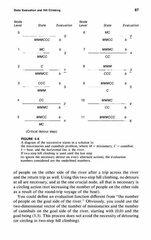
State Evaluation and Hill Climbing 87

Node Node Level Sta te Evalua tion Level Sta te Evalua tion

0 6 MC 0 2

MMMGGG b MMGG b

MG b 7 MMMG b 2 4

MMGG GG

2 G 8 MMM 3

MMMGG b GGG b

3 GGG b 9 MMMGG b 3 5

MMM G

4 GG 1 0 MMMG 2 4

MMMG b GG b

5 MMGG b 1 1 MMMGGG b 4 6

MG

(Crit ical detour step)

AGURE 5-8 A diagram of the successive states in a solution to the missionaries and cannibals problem, where M = miss ionary, C = cannibal , h = boat , and the horizontal l ine is the river. If two-step hi l l c l imbing is used until the last step (to ignore the necessary detour on every alternate action), the evaluation numbers considered are the underlined numbers.

of people on the other side of the river after a trip across the river and the return trip as wel l . U sing this two-step hill c l imbing, no detours at all are necessary, and at the one crucial node, all that is necessary is a circl ing action (not increasing the number of people on the other s ide as a result of the round-trip voyage of the boat ) .

You could define an evaluation function different from "the number of people on the goal side of the river. " Obviously, you could use the two-dimensional vector of the number of missionaries and the number of cannibals on the goal side of the river, starting with (0,0) and the goal being ( 3 ,3 ) . This process does not avoid the necessity of detouring (or circling in two-step hill c l imbing).

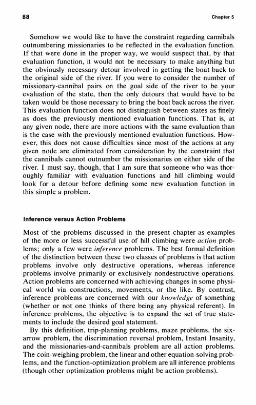
88 Chapter 5

Somehow we would l ike to have the constraint regarding cannibals outnumbering missionaries to be reflected in the evaluation function. If that were done in the proper way, we would suspect that , by that evaluation function, it would not be necessary to make anything but the obviously necessary detour involved in getting the boat back to the original side of the river. If you were to consider the number of missionary-cannibal pairs on the goal side of the river to be your evaluation of the state, then the only detours that would have to be taken would be those necessary to bring the boat back across the river. This evaluation function does not d istinguish between states as finely as does the previously mentioned evaluation functions. That is, at any given node, there are more actions with the same evaluation than is the case with the previously mentioned evaluation functions. How­ever, thi s does not cause difficulties since most of the actions at any given node are el iminated from consideration by the constraint that the cannibals cannot outnumber the missionaries on either side of the river. I must say, though, that I am sure that someone who was thor­oughly familiar with evaluation functions and hi l l c l imbing would look for a detour before defining some new evaluation function in this s imple a problem.

Inference versus Action Problems

Most of the problems discussed in the present chapter as examples of the more or less successful use of hill c l imbing were action prob­lems ; only a few were inference problems. The best formal definition of the distinction between these two classes of problems i s that action problems involve only destructive operations , whereas inference problems involve primarily or exclusively nondestructive operations. Action problems are concerned with ach ieving changes in some physi­cal world via constructions , movements, or the l ike. By contrast, inference problems are concerned with our knowledge of something (whether or not one thinks of there being any physical referent) . In inference problems, the objective is to expand the set of true state­ments to include the desired goal statement.

By this definition, trip-planning problems, maze problems, the six­arrow problem, the d iscrimination reversal problem, Instant Insanity, and the miss ionaries-and-cannibals problem are all action problems. The coin-weighing problem, the l inear and other equation-solving prob­lems, and the function-optimization problem are all inference problems (though other optimization problems might be action problems) .

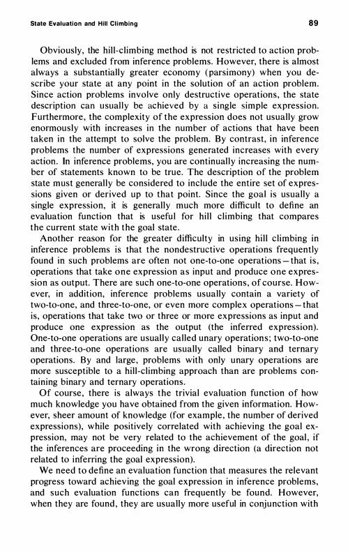
State Evaluation and Hill Climbin g 89

Obviously, the hi l l -cl imbing method is not restricted to action prob­lems and excluded from inference problems. However, there is almost always a substantial ly greater economy (parsimony) when you de­scribe your state at any point in the solution of an action problem. Since action problems involve only destructive operations , the state description can u sual l y be achieved by a s ingle simple expression. Furthermore , the complexity of the expression does not usually grow enormously with increases in the number of actions that have been taken in the attempt to solve the problem. By contrast, in inference problems the number of expressions generated increases with every action . In inference problems, you are continual ly increasing the num­ber of statements known to be true. The description of the problem state must general ly be considered to include the entire set of expres­sions given or derived up to that point. Since the goal i s usually a single expression, it is general ly much more difficult to define an evaluation function that is usefu l for hi l l c l imbing that compares the current state with the goal state .

Another reason for the greater d ifficulty in using hi l l c l imbing in inference problems i s that the nondestructive operations frequently found in such problems are often not one-to-one operations - that i s , operations that take one expression as input and produce one expres­sion as output. There are such one-to-one operations , of course. How­ever, in addition, inference problems usually contain a variety of two-to-one, and three-to-one, or even more complex operations - that is , operations that take two or three or more expressions as input and produce one expression as the output (the inferred expression) . One-to-one operations are usual ly cal led unary operations ; two-to-one and three-to-one operations are usually called b inary and ternary operations. By and large , problems with only unary operations are more susceptible to a hi l l -cl imbing approach than are problems con­taining binary and ternary operations .

Of course , there is always the trivial evaluation function of how much knowledge you have obtained from the given information. How­ever, sheer amount of knowledge (for example , the number of derived expressions), while positively correlated with achieving the goal ex­pression, may not be very related to the achievement of the goal , if the inferences are proceeding in the wrong direction (a direction not related to inferring the goal expression).

We need to define an evaluation function that measures the relevant progress toward achiev ing the goal expression in inference problems, and such evaluation functions can frequently be found. However, when they are found , they are usually more useful in conjunction with

90 Chapter 5

the subgoal method (to be discussed in the following chapter) than they are with hi l l c l imbing. The reason is that usually a sequence of several actions is required to achieve an expression that moves the evaluation function in the d irection of the evaluation characteristic of the goal . Most of the single actions taken in reaching each successive subgoal cannot themselves be identified as reducing the distance to the goal in terms of the goal evaluation function.

However, in these cases , if we define evaluation functions relevant for reaching each successive subgoal , then conceivably in a very large proportion of inference problems it is possible to use the hil l-cl imbing method to achieve various subgoals . Some examples of this combined use of hill cl imbing and subgoal methods will be discussed in the mathematics , science , and engineering problems of Chapter 1 1 .

6

Subgoals

THEORY

A problem-solving method that is important but difficult to master is that of defining subgoals in order to faci l itate solving the original problem. This method is sometimes called "analyzing a problem into subproblems," or "breaking up a problem into parts ." In essence, the purpose is to replace a s ingle difficult prob lem wi th two or more simpler problems.

Of course , if you already know how to solve some of the sub­problems, or if some of them are analogous to problems you already know how to solve, then obviously it might be easier to solve the set of simpler problems than the single original problem.

However, the fact that it is advantageous to break up a problem into subproblems does not mean you must be more fami liar with the sub­problems than with the original problem. One way to see the advantage of defining subgoals is to look at the fol lowing analysis of the state­action tree for a problem ( 1 ) with m alternative actions at each node and (2) a sequence of n actions being necessary for solution.

Let us assume that we know that the solution to some problem wil l require a sequence of n actions (or less) . By systematic trial and error there are m" alternative paths (action sequences) to be investigated

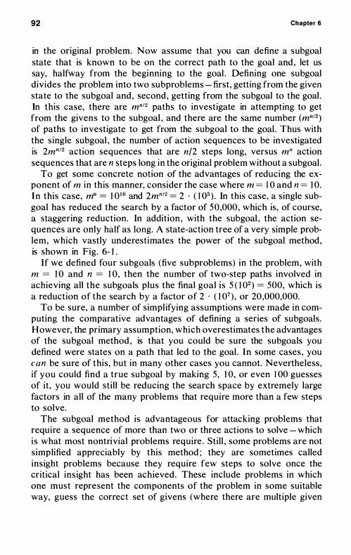
92 Chapter 6

in the original problem. Now assume that you can define a subgoal state that is known to be on the correct path to the goal and , let us say, halfway from the beginning to the goal . Defining one subgoal divides the problem into two subproblems - first, getting from the given state to the subgoal and , second , getting from the subgoal to the goal . In this case, there are mn/2 paths to investigate in attempting to get from the givens to the subgoal , and there are the same number (mn/2 ) of paths to investigate to get from the subgoal to the goal . Thus with the single subgoal , the number of action sequences to be investigated is 2mn/2 action sequences that are n/2 steps long, versus mil action sequences that are n steps long in the original problem without a subgoal .

To get some concrete notion of the advantages of reducing the ex­ponent of m in this manner, consider the case where m = 1 0 and n = 1 0. In this case, mn = 1 010 and 2mn/2 = 2 . ( 1 05 ) . In this case, a single sub­goal has reduced the search by a factor of 50,000, which is, of course, a staggering reduction. In addition , with the subgoal , the action se­quences are only half as long. A state-action tree of a very simple prob­lem, which vastly underestimates the power of the subgoal method, is shown in Fig. 6- 1 .

If we defined four subgoals (five subproblems) in the problem, with m = 1 0 and n = 1 0 , then the number of two-step paths involved in achieving all the subgoals plus the final goal i s 5 ( 1 02 ) = 500, which is a reduction of the search by a factor of 2 . ( 1 07 ) , or 20 ,000,000.

To be sure, a number of simpl ifying assumptions were made in com­puting the comparative advantages of defining a series of subgoals . However, the primary assumption, which overestimates the advantages of the subgoal method , is that you could be sure the subgoals you defined were states on a path that led to the goal . In some cases , you can be sure of this , but in many other cases you cannot. Nevertheless, if you could find a true subgoal by making 5, 1 0, or even 1 00 guesses of it , you would sti l l be reducing the search space by extremely large factors in all of the many problems that require more than a few steps to solve.

The subgoal method is advantageous for attacking problems that require a sequence of more than two or three actions to solve - which i s what most nontrivial problems require . Still , some problems are not simplified appreciably by this method ; they are sometimes called ins ight problems because they require few steps to solve once the critical ins ight has been achieved . These include problems in which one must represent the components of the problem in some suitable way, guess the correct set of givens (where there are multiple given

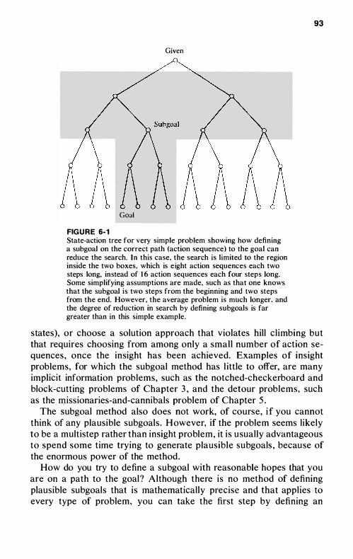
Given

Goal

FIG U R E 6·1 State-action tree for very simple problem showing how defining a subgoal on the correct path (action sequence) to the goal can reduce the search. I n this case, the search is l imited to the region inside the two boxes, which is e ight action sequences each two steps long, instead of 1 6 action sequences each four steps long. Some simplifying assumptions are made, such as that one knows that the subgoal i s two steps from the beginning and two steps from the end. However, the average problem is much longer, and the degree of reduction in search by defining subgoals is far greater than in this simple example.

93

states), or choose a solution approach that violates hill c l imbing but that requires choosing from among only a small number of action se­quences , once the insight has been achieved. Examples of insight problems, for which the subgoal method has l ittle to offer, are many implicit information problems, such as the notched-checkerboard and block-cutting problems of Chapter 3 , and the detour problems, such as the missionaries-and-cannibals problem of Chapter 5 .

The subgoal method also does not work, of course, i f you cannot think of any plausible subgoals . However, if the problem seems likely to be a multistep rather than insight problem, it i s usually advantageous to spend some time trying to generate plausible subgoals , because of the enormous power of the method.

How do you try to define a subgoal with reasonable hopes that you are on a path to the goal? Although there is no method of defining plausible subgoals that is mathematically precise and that applies to every type of problem, you can take the first step by defining an

94 Chapter 6

evaluation function over d ifferent problem states , as was done as a necessary precondition in applying the hil l-cl imbing method . Having done this, you can recognize a plausible subgoal as a problem state with an evaluation part way between the given state and the goal state. I f the evaluation function is multidimensional , then such a subgoal might have the goal values on some, but not al l , of the dimensions. Or it might just have values closer to the goal values on some, or even all , of the dimensions.

Defining an evaluation function over problem states provides not only a way to recognize a plausible subgoal but also a way to generate or define plausible subgoals . Evaluation functions are single valued in the d irection from a problem state to an evaluation vector for the problem state . (Multidimensional evaluation functions are still single valued so long as only one distinct evaluation vector is associated with each distinct problem state . ) The inverse function may be multivalued , but that does not seriously reduce the value of this approach to generating plausible subgoals .

It may be that subgoals can always be determined to have inter­mediate values between the given and goal state according to some explicitly defined evaluation function. However, a person may fre­quently define subgoals without being able to state explicitly any relevant evaluation function. Thus , this book will generally discuss the appl ication of the subgoal method to problems without attempting to describe any formal evaluation function.

I n general , there are a multiplicity of plausible subgoals , some on a correct path to the goal and some not. As mentioned , even if the probability of a plausible subgoal being a true subgoal is only 0. 1 or 0.0 1 , the method is stil l reducing the search by an enormous factor in most problems. In any event, it i s usual ly not very difficult to con­jecture a variety of reasonably plausible subgoals , but the l ikelihood of defining a good subgoal will depend upon how good an evaluation function you have defined over problem states . In turn , how good your evaluation function is, how suitable it is to solving the problem at hand, often depends upon how adequately you represented the in­formation in the problem (discussed in Chapters 3 and 1 0) , the defining of macroactions , and the use of various other problem-solving methods. Problem-solving methods are generally used in combination , and the combined power of several methods in reducing the search space can result in very fast solution of many problems with l ittle trial-and-error search being required.

When you have defined two or more subgoals to be achieved in get­ting from the given state to the goal , you can make a logical distinction

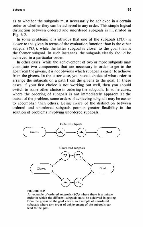
Subgoals 95

as to whether the subgoals must necessarily be ach ieved in a certain order or whether they can be achieved in any order. This simple logical d istinction between ordered and unordered subgoals i s i l lustrated in Fig. 6-2.

In some problems it i s obvious that one of the subgoals (SG , ) is closer to the given in terms of the evaluation function than i s the other subgoal (SG2 ) , while the latter subgoal i s closer to the goal than is the former subgoal . In such instances , the subgoals c learly should be achieved in a particular order.

In other cases, while the achievement of two or more subgoals may constitute two components that are necessary in order to get to the goal from the givens, it is not obvious which subgoal is easier to achieve from the givens. In the latter case , you have a choice of what order to arrange the subgoals on a path from the givens to the goal. In these cases, if your first choice i s not working out well, then you should switch to some other choice in ordering the subgoals . In some cases, where the ordering of subgoals i s not immediately apparent at the outset of the problem, some orders of achieving subgoals may be easier to accomplish than others. Being aware of the distinction between ordered and unordered subgoals permits greater flexibi lity in the solution of problems involving unordered subgoals .

Ordered subgoals

( Givens >--e -®-( GOal ) Unordered subgoals

FIG U R E 6-2 An example of ordered subgoals (SG i) where there is a unique order in which the different subgoals must be achieved in getting from the givens to the goal versus an example of unordered subgoals where any order of ach ievement of the subgoals can lead to the goal .

96 Chapter 6

If you have defined n subgoals (whether ordered or unordered) , you have automatical ly defined n + 1 subproblems to be solved - namely, getting from the givens to one of the subgoals , getting from the first subgoal to the second subgoal , and so on, from the nth subgoal to the goal . Whether any particular ordering of the subgoals is required by the original evaluation function or is optional by that evaluation function, you may often be free to choose to work on any l ink in the chain first, second, and so on. By and large , it is advantageous to start with a subproblem of getting from the givens to one of the subgoals , or else to work on the problem of getting from one of the subgoals to the goal , because subgoal s are frequently not ful ly defined problem states . I t is usually preferable to work on a subproblem in which either the beginning or end state is completely specified . In most problems, this means starting from the givens is preferable, though in some cases working backward from the goal may be just as good or better. An additional advantage of starting with the givens is that you are simultaneously drawing inferences (see discussion of this method in Chapter 3) that you know is expanding the information you have available for the solution of the problem, no matter what the ultimate success of the particular subgoal approach that you have taken. If you begin working on other subproblems that do not start from the given state , then a failure using the subgoal approach may not have generated equivalently useful information as that which would have been generated by starting from the givens. All this is perhaps rela­tively obvious , but it is nevertheless important to bear in mind.

APPLICATIONS

Planning a trip across the country is a problem to which the subgoal method can be applied in a relatively trivial manner. If you wanted to travel from San Francisco to New York City, you might select Denver and Chicago as subgoals . Selection of such reasonable subgoals de­pends upon having an evaluation function defined over such cities (such as their two-dimensional coordinates on a map) , which indicates that Denver and Chicago have intermediate values on the east-west coordinate compared to San Francisco and New York. In this case , it is primarily one of the two dimensions of the evaluation function that needs to be altered to get from the given state to the goal . But in going from Spokane , Washington , to Miami , Florida, by way of Denver and Memphis, Tennessee, you are substantial ly altering the values on both d imensions in going from the given state to the goal . Obviously, the subgoals are ordered in these trip-planning problems.

Subgoals 97

As an example of a problem that i s extremely easy to solve us ing the subgoal method (with unordered subgoals) , consider the following :

A light plane carrying three men crashes in the desert . The men decide that their best chance for survival consists of each of them setting across the desert in different directions in hopes that one of the directions wil l pass by a sufficient number of oases to permit that man to reach civiliza­tion and get help for the others. Before going their separate ways across the desert , they are faced with the problem of achieving an equal division of their stock of water and canteens . They have in their possession five canteens ful l of water, five canteens half-full of water, and five empty canteens. All canteens are the same size. Since water-carrying capacity is important should a man reach an oasis, they wish to divide both their supply of water and the number of canteens equally among themselves. How can they achieve this?

Stop reading and attempt to solve th is problem. If you were unable to solve it , consider the fol lowing hints . You

might original ly define three unordered subgoals consisting of attempt­ing to divide the ful l canteens evenly among the three men, dividing the half-ful l canteens evenly among the three men , and dividing the empty canteens evenly among the three. I t is immediately obvious that this subgoal approach wil l not work. An alternative definition of sub­goals involves first making the inferences that the total quantity of water is 5 + � or 7 4 canteens ful l of water and that the total number of canteens equals 1 5 . From this you can conclude that, in the goal state , each person wil l have 2 4 canteens ful l of water and 5 canteens . In es­sence, this defines a six-dimensional vector evaluation function such that in the given state each of the three persons has zero water and zero canteens and in the goal state each person has 24 canteens ful l of water and 5 canteens. If you have not solved the problem, stop read­ing and attempt to define relevant subgoals .

The relevant subgoals are to attempt to give first one of the men (it obviously does not matter which one) 24 canteens ful l of water d is­tributed among five canteens. There are a number of ways of doing this , only one of which wil l make it impossible to achieve the other two subgoals of giving 2 4 canteens ful l of water in 5 canteens to each of the other two men. The only way that prevents achievement of the goal is to give the first man the entire set of half-ful l canteens. Any other method of giving the first man 24 canteens ful l of water and 5 canteens wil l permit achievement of the remaining two subgoals - namely, give the first man I ful l canteen of water, 3 half fu ll canteens of water, and I empty canteen , or give the first man 2 ful l canteens of water, 1 half ful l canteen of water, and 2 empty canteens . Once the first subgoal has

98 Chapter 6

been achieved, it is trivially obvious whether or not it is possible to achieve the second and third subgoals .

Another problem that i l lustrates the power of the repeated use of the subgoal method is the fol lowing :

Nine men and two boys want to cross a river, using an inflatable raft that will carry either one man or the two boys. How many times must the boat cross the river in order to accomplish this goal? (A round trip equals two crossings. )

Stop reading and try to solve the problem, using the subgoal method. Define as a subgoal the problem of getting one man across the river

and getting the boat back to the starting side. Stop reading and attempt to solve the problem, if you have not already.

It takes exactly four crossings to get one man across the river and return the boat to the original side. First, the two boys cross the river in the boat, then one boy takes the boat back to the original side of the river, then a man takes the boat across the river, and then the second boy takes the boat back to the original side of the river. These four crossings put both boys and the boat in the same position they were when they transported the first man across the river. Thus , to transport all nine men across the river wi l l require 9 x 4 or 3 6 one-way crossings. At that point, both boys will be on the original side of the river with the boat, and one additional crossing wi l l be required for them to get to the goal side of the river with the boat. Thus , a total of 37 one-way crossings are required in all .

A n example of a somewhat similar subgoal problem in a probability context is provided by the fol lowing example :

The ace, 2 , 3 , 4, 5 , 6, 7 , and 8 of hearts are placed face up in a row on the table . Then a pack of eight cards containing the ace, 2 , 3 , 4 , 5 , 6 , 7 , and 8 of spades are shuffled and placed in front of the player. As each succes­sive spade is turned over, the corresponding heart is removed from the row. What is the probability that all the hearts can be removed without a break (hole) ever occurring in the row of hearts?

Stop reading and try to solve the problem. Consider as a subgoal the probabi l ity that the first removed heart

does not cause a break in the row. Stop reading and try to solve the problem, us ing this subgoal .

The probability of achieving the first subgoal (removing one heart without producing a break in the row) is exactly � . This probability results from the fact that there are two end positions to the row, and

Subgoals 99

only the two cards in these end positions may be removed without causing a break. Since there are eight cards in the row, the probability is �. If you d id not solve the problem before , stop reading and try to solve the original problem, having achieved the solution to the subgoal.

Once the first sub goal has been achieved of drawing one card from the end of each row (and its probabi l ity has been determined) , the second subgoal should be to compute the probabi l ity that the second card will be removed from the end of the row. If the first subgoal has been successful ly achieved, there are stil l two cards at the ends, but now only seven cards in toto. Thus , the probabi l ity of successful ly re­moving a second card from the ends of the row is �. If you have not yet solved the entire problem, stop reading and try to complete the rest of the solution on your own.

Continue in th is way, defining successive subgoals of removing cards from either end of the row until all cards have been removed. The probabil ity that each subgoal will be successful ly achieved with a random shuffling of the pack of spades is evidently � . � . i . � . � . i . � , or :1:5 ' The probabil ity of successful achievement of the entire set of necessary subgoals is simply the product of the probabi l ities of achieving each successive sub goal . Note that th is probabi l ity problem represents a rather interesting variation in the use of the subgoal method , since there are, in essence, two paral le l sets of subgoals in­volved in the problem. On the one hand , there is the series of subgoal s of removing cards from an end of the row, progressively reducing the row in length without creating a hole. On the other hand, there is the series of subgoals of computing the probabilities of achieving each of these subgoals .

Now consider this rather different problem (previously discussed in Chapter 3 ) , which also i l lu strates the use of the subgoal method :

Wanda the witch agrees to trade one of her magic broomsticks to Gaspar the ghost in exchange for one of his gold chains . Gaspar is somewhat skeptical that the broomstick is in working order and ins ists on a guaran­tee equal to the number of l inks in the gold chain. As a guarantee , he insists on paying by the installment plan , one gold link per day until the end of the 63-day period, with the balance to be forfeit if the broomstick malfunctions during the guarantee period. Wanda agrees to this arrange­ment , but ins i sts that the insta l lment payment be effected by cutt ing no more than three l inks in the gold chain . Can th is cutting be done, and , if so, what links in the chain should be cut? The chain in i t ially consi sts of 63 closed gold l inks arranged in a s imple linear order (not closed into a c ircle).

Stop reading and try to solve the problem.

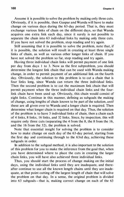
100 Chapter 6

Assume it is possible to solve the problem by making only three cuts. Obviously, if it is possible, then Gaspar and Wanda wil l have to make change on various days during the 63 -day period . That is , they must exchange various links of chain on the different days , so that Wanda acquires one extra l ink each day, since it surely is not possible to separate the chain into 63 individual l inks by making only three cuts. If you have not solved the problem, stop reading and try again.

Stil l assuming that it is possible to solve the problem, note that, if it is possible, the solution wil l result in creating at least three single l inks of chain , as well as various other longer l inks of chain. If you have not solved the problem so far, stop reading and try again.

Having three individual chain l inks wil l permit payment of one link per day from days 1 to 3. Now as the first subproblem, you should determine the longest link chain that can be used with Wanda making change , in order to permit payment of an additional link on the fourth day. Obviously, the solution to this problem is to cut a chain that is four l inks long, since Wanda can return the three individual l inks. Then the second problem is to cut the maximum link chain that will permit payment when the three individual chain l inks and the four­l ink chain have been used up. Obviously, this chain would consist of eight l inks . Continue in this manner, defining as subgoals the making of change , us ing lengths of chain known to be part of the solution , until these are all given over to Wanda and a longer chain is required. Then determine what longer chain i s required on that day. Thus, the solution of the problem is to have 3 individual l inks of chain, then a chain each of 4 l inks, 8 l inks, 1 6 l inks, and 32 l inks . Since, by inspection, this will require only three cuts (separating the 4 from the 8 , the 8 from the 1 6, and the 1 6 from the 3 2) , the problem is solved.

Note that essential insight for solving the problem is to consider how to make change on each day of the 63 -day period , starting from the first day and continuing through to the 63rd day, achieving these subgoals in order.

In addition to the subgoal method , it is also important te> the solution of this problem for you to make the inference from the goal that, when you have determined where to place the cuts in creating the larger chain l inks, you will have also achieved three individual l inks.

Thus , you should start the process of change making on the initial days , using the individual l inks unti l they are inadequate, and there­after continue to use all the known length chains until they are inade­quate , at that point cutting off the largest length of chain that wil l solve the problem on that day. In a sense, the original problem is divided into 63 subgoals - that is, making correct change on each of the 63

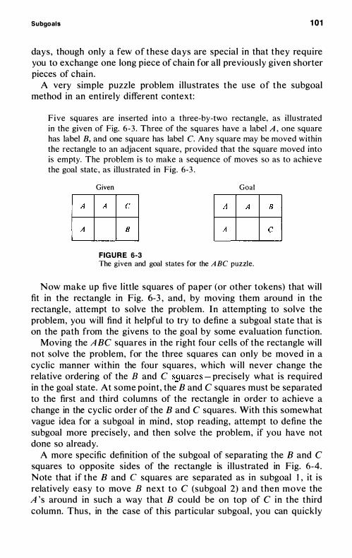
Subgoals 101

days , though only a few of these days are special in that they require you to exchange one long piece of chain for all previously given shorter pieces of chain .

A very simple puzzle problem i l lustrates the use of the subgoal method in an entirely different context :

Five squares are inserted into a three-by-two rectangle, as illustrated in the given of Fig. 6 -3 . Three of the squares have a label A , one square has label B, and one square has label C. Any square may be moved within the rectangle to an adjacent square , provided that the square moved into is empty. The problem is to make a sequence of moves so as to achieve the goal state , as illustrated in Fig. 6-3 .

Given

� �

FIG U R E 6-3

Goal

� �

The given and goal states for the A Be puzzle.

Now make up five l ittle squares of paper (or other tokens) that will fit in the rectangle in Fig. 6-3 , and , by moving them around in the rectangle, attempt to solve the problem. In attempting to solve the problem, you will find it helpful to try to define a subgoal state that is on the path from the givens to the goal by some evaluation function.

Moving the A Be squares in the right four cel ls of the rectangle will not solve the problem, for the three squares can only be moved in a cyclic manner within the four squares , which wil l never change the relative ordering of the B and e sguares - precisely what is required in the goal state . At some point, the B and e squares must be separated to the first and third columns of the rectangle in order to achieve a change in the cyclic order of the B and e squares . With this somewhat vague idea for a subgoal in mind , stop reading, attempt to define the subgoal more precisely, and then solve the problem, if you have not done so already.

A more specific definition of the subgoal of separating the B and e squares to opposite sides of the rectangle is i l lustrated in Fig. 6-4. Note that if the B and e squares are separated as in subgoal 1 , it is relatively easy to move B next to e (subgoal 2) and then move the A 's around in such a way that B could be on top of e in the third column. Thus, in the case of this particular subgoal , you can quickly

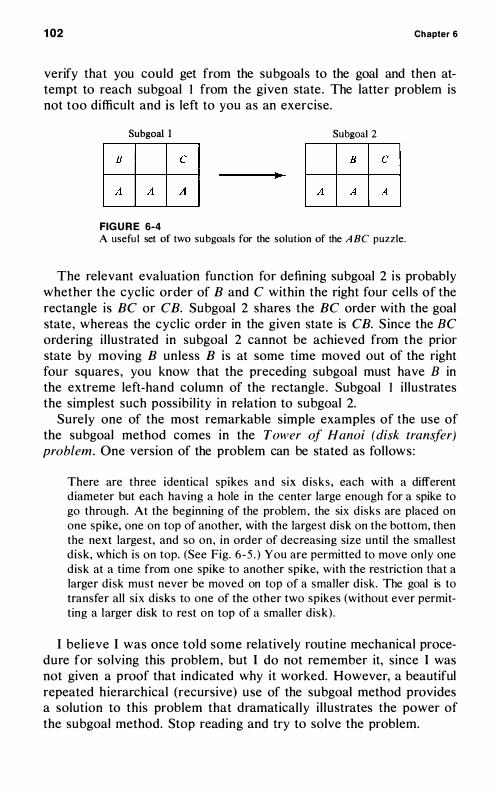
102 Chapter 6

verify that you could get from the subgoals to the goal and then at­tempt to reach subgoal 1 from the given state . The latter problem is not too difficult and is left to you as an exercise.

Subgoal l

ITE �

FIG U R E 6-4

Subgoal 2

LEE] �

A usefu l set of two subgoals for the solution of the A BC puzzle.

The relevant evaluation function for defining subgoal 2 i s probably whether the cycl ic order of B and C within the right four cel ls of the rectangle is BC or CB. Subgoal 2 shares the BC order with the goal state , whereas the cyclic order in the given state is CB. S ince the BC ordering i l lustrated in subgoal 2 cannot be achieved from the prior state by moving B unless B is at some time moved out of the right four squares , you know that the preceding subgoal must have B in the extreme left-hand column of the rectangle . Subgoal 1 i l lustrates the simplest such possibil ity in relation to subgoal 2.

Surely one of the most remarkable simple examples of the use of the subgoal method comes in the Tower of Hanoi (disk transfer) problem. One version of the problem can be stated as follows :

There are three identical spikes and s ix d i sks , each with a different diameter but each having a hole in the center large enough for a spike to go through. At the beginning of the problem , the six d isks are placed on one spike, one on top of another, with the largest disk on the bottom, then the next largest, and so on, in order of decreasing size until the smallest disk, which is on top. (See Fig. 6 -5 . ) You are permitted to move only one d isk at a time from one spike to another spike, with the restriction that a larger disk must never be moved on top of a smaller disk. The goal is to transfer all six disks to one of the other two spikes (without ever permit­ting a larger disk to rest on top of a smaller d isk) .

I bel ieve I was once told some relatively routine mechanical proce­dure for solving this problem, but I do not remember it, since I was not given a proof that indicated why it worked. However, a beautiful repeated hierarchical (recursive) use of the subgoal method provides a solution to this problem that dramatical ly i l lustrates the power of the subgoal method. Stop reading and try to solve the problem.

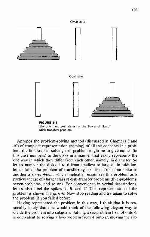
Given state

Goal state

FIG U R E 6-5 The given and goal states for the Tower of Hanoi (disk transfer) problem.

1 03

Apropos the problem-solving method (discussed in Chapters 3 and 1 0) of complete representation (naming) of all the concepts in a prob­lem, the first step in solving this problem might be to give names (in this case numbers) to the disks in a manner that easily represents the one way in which they differ from each other, namely, in diameter. So let us number the disks I to 6 from smallest to largest. In addition, let us label the problem of transferring six disks from one spike to another a six-problem, which implicitly recognizes this problem as a particular case of a larger class of disk-transfer problems (five-problems, seven-problems, and so on) . For convenience in verbal descriptions , let us also label the spikes A , B , and C. This representation of the problem is shown in Fig. 6 -6. Now stop reading and try again to solve the problem, if you failed before .

Having represented the problem in this way, I think that it is rea­sonably likely that one would think of the following e legant way to divide the problem into subgoals . Solving a s ix-problem from A onto C is equivalent to solving a five-problem from A onto B , moving the six-

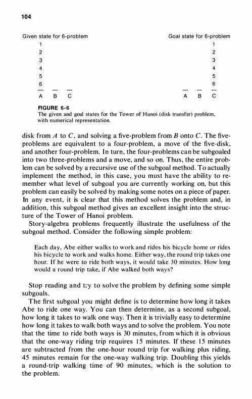
104

G iven state for 6-pro blem

1

Goal state for 6-problem

1

2

3

4

5

6

A B c

R G U R E 6 - 6

A

2

3

4

5

6

B C

The given and goal states for the Tower of H anoi (disk transfer) problem, with numerical representation.

disk from A to C, and solving a five-problem from B onto C. The five­problems are equivalent to a four-problem, a move of the five-disk, and another four-problem. In turn , the four-problems can be subgoaled into two three-problems and a move, and so on. Thus , the entire prob­lem can be solved by a recursive use of the subgoal method . To actually implement the method , in this case , you must have the ability to re­member what level of subgoal you are currently working on, but this problem can easily be solved by making some notes on a piece of paper. In any event, it is c lear that this method solves the problem and , in addition, this subgoal method gives an excellent insight into the struc­ture of the Tower of Hanoi problem.

Story-algebra problems frequently i l lustrate the usefulness of the subgoal method . Consider the following simple problem:

Each day, Abe either walks to work and rides his bicycle home or rides his bicycle to work and walks home. Either way, the round trip takes one hour. I f he were to ride both ways, i t would take 30 minutes. How long would a round trip take, if Abe walked both ways?

Stop reading and try to solve the problem by defining some simple subgoals .

The first subgoal you might define i s to determine how long it takes Abe to ride one way. You can then determine, as a second subgoal , how long it takes to walk one way. Then it is trivially easy to determine how long it takes to walk both ways and to solve the problem. You note that the time to ride both ways is 30 minutes , from which it is obvious that the one-way riding trip requires 1 5 minutes. If these 1 5 minutes are subtracted from the one-hour round trip for walking plus riding, 45 minutes remain for the one-way walking trip. Doubling this yields a round-trip walking time of 90 minutes , which is the solution to the problem.

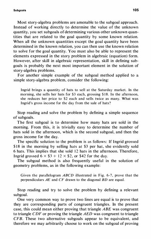
Subgoals 105

Most story-algebra problems are amenable to the subgoal approach . Instead of working directly to determine the value of the unknown quantity, you set subgoals of determining various other unknown quan­tities that are related to the goal quantity by some known relation. When all the unknown quantities except the goal quantity have been determined in the known relation, you can then use the known relation to solve for the goal quantity. You must also be able to represent the elements expressed in the story problem in algebraic (equation) form. However, after skill in algebraic representation, skill in defining sub­goal s is probably the next most important element in the solution of story-algebra problems.

For another simple example of the subgoal method applied to a simple story-algebra problem, consider the following:

I ngrid brings a quantity of hats to sell at the Saturday market . In the morning, she sells her hats for $3 each, gross ing $ 1 8 . I n the afternoon, she reduces her price to $2 each and sells twice as many. What was I ngrid's gross income for the day from the sale of hats?

Stop reading and solve the problem by defining a simple sequence of subgoals .

The first subgoal is to determine how many hats are sold in the morning. From this , it is trivially easy to determine the number of hats sold in the afternoon, which is the second subgoal , and then the gross income for the day.

The specific solution to the problem is as follows : If I ngrid grossed $ 1 8 in the morning by sel l ing hats at $3 per hat , she evidently sold 6 hats . This implies that she sold 1 2 hats in the afternoon. Therefore , I ngrid grossed 6 x $3 + 1 2 x $ 2 , or $42 for the day.

The subgoal method is also frequently usefu l in the solution of geometry problems, as in the following example :

G iven the parallelogram A BCD i l lustrated in F ig . 6 -7 , prove that the perpendiculars AE and CF drawn to the diagonal BD are equal.

Stop reading and try to solve the problem by defining a relevant subgoal .

One very common way to prove two l ines are equal is to prove that they are corresponding parts of congruent triangles . In the present case, this could mean either proving that triangle A BE was congruent to triangle CDF or proving the triangle A ED was congruent to triangle CFB. These two alternative subgoals appear to be equivalent, and therefore we may arbitrarily choose to work on the subgoal of proving

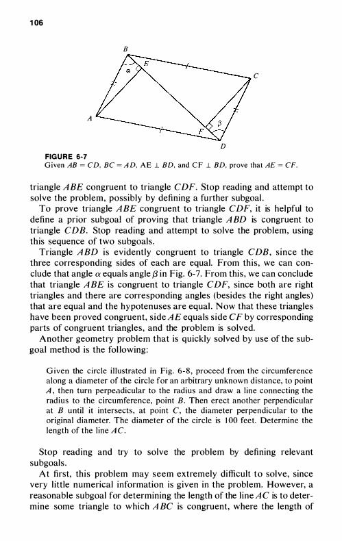
1 06

B

C

A

D FIG U R E 6-7 G iven AB = CD. BC = A D. A E � BD. and C F � BD. prove that AE = CF.

triangle A BE congruent to triangle CDF. Stop reading and attempt to solve the problem, possibly by defining a further subgoal .

To prove triangle A BE congruent to triangle CDF, it is helpful to define a prior subgoal of proving that triangle A BD is congruent to triangle CDB. Stop reading and attempt to solve the problem, using this sequence of two subgoals .

Triangle A BD is evidently congruent to triangle CDB, s ince the three corresponding sides of each are equal. From this , we can con­clude that angle a equals angle {3 in Fig. 6-7. From this , we can conclude that triangle A BE is congruent to triangle CDF, since both are right triangles and there are corresponding angles (besides the right angles) that are equal and the hypotenuses are equal . Now that these triangles have been proved congruent, s ide A E equals s ide C F by corresponding parts of congruent triangles , and the problem is solved.

Another geometry problem that is quickly solved by use of the sub­goal method is the fol lowing :

G iven the circle illustrated in Fig. 6 - 8 , proceed from the circumference along a diameter of the circle for an arbitrary unknown d istance, to point A , then turn perpeadicular to the radius and draw a line connecting the radius to the circumference, point B. Then erect another perpendicular at B until it intersects , at point C, the diameter perpendicular to the original d iameter. The diameter of the circle is 1 00 feet . Determine the length of the line A C.

Stop reading and try to solve the problem by defining relevant subgoals .

At first, this problem may seem extremely difficult to solve, since very l ittle numerical information is given in the problem. However, a reasonable subgoal for determining the length of the l ine A C is to deter­mine some triangle to which A BC is congruent, where the length of

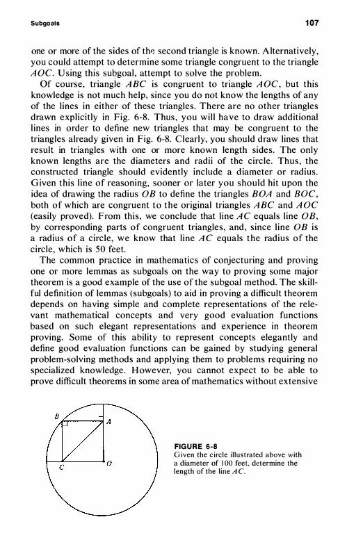
Subgoals 107

one or more of the sides of thp. second triangle is known. A lternatively, you could attempt to determine some triangle congruent to the triangle A OC. U sing this subgoal , attempt to solve the problem.

Of course, triangle A BC is congruent to triangle A �C, but this knowledge is not much help, since you do not know the lengths of any of the l ines in either of these triangles . There are no other triangles drawn explicitly in Fig. 6-8. Thus , you wil l have to draw additional l ines in order to define new triangles that may be congruent to the triangles already given in Fig. 6-8. Clearly, you should draw lines that result in triangles with one or more known length sides . The only known lengths are the diameters and radii of the circle . Thus , the constructed triangle should evidently include a d iameter or radius . Given this l ine of reasoning, sooner or later you should hit upon the idea of drawing the radius DB to define the triangles BOA and BOC, both of which are congruent to the original triangles A BC and A OC (easily proved). From this , we conclude that l ine A C equal s l ine DB, by corresponding parts of congruent triangles , and , since l ine DB is a radius of a circle, we know that l ine A C equals the radius of the circle, which is 50 feet.

The common practice in mathematics of conjecturing and proving one or more lemmas as subgoals on the way to proving some major theorem is a good example of the use of the subgoal method. The skill­ful definition of lemmas (subgoals) to aid in proving a difficult theorem depends on having simple and complete representations of the rele­vant mathematical concepts and very good evaluation functions based on such elegant representations and experience in theorem proving. Some of this ability to represent concepts elegantly and define good evaluation functions can be gained by studying general problem-solving methods and applying them to problems requiring no specialized knowledge . However, you cannot expect to be able to prove difficult theorems in some area of mathematics without extensive

FIG U R E 6-8 G iven the c ircle i l lustrated above with a diameter of 1 00 feet, determine the length of the l ine A c.

1 08 Chapter 6

studying of the concepts, assumptions , operations , and so on, in that area. To solve problems in a specialized area of knowledge , one must have learned certain elegant ways of representing concepts in that area. This knowledge is often required in order to define good evalua­tion functions for use in hill c l imbing and the subgoal method.

Another mathematical proof technique that is an ingenious use of the subgoal method is mathematical induction . Mathematical induc­tion can be used to prove theorems that in some way involve natural numbers ( positive integers). Let the goal expression you are trying to prove be represented by E(n), where n stands for any natural num­ber (n 2 I ) . The problem of proving E(n) true for any natural number, n , can be divided into two subproblems : first, proving E(n) true for n = I , and , second, proving that if E(n - 1 ) is true, then E(n) is true.

For example, consider a mathematical induction proof of the theorem that the sum of the first n positive integers, I?= 1 i, is n(n + 1 )/2 :

( 1 ) 2: � = 1 i = 1 = 1 . t so true for n = 1 .

(n - I ) n (2) Assume true for (n - I ) : 2::'=-/ i =

2

( 3 ) Add n to both sides : 2: 7= 1 i = (n -

21 ) n

+ n

(4) . (n - I ) n + 2n Put over common denominator: 2::'= 1 1 = 2

(5) F t · � /I • _ n (n - 1 + 2) ac or. L. i = 1 1 -2

(6) Simplify : 2:;'= 1 . n (n + l ) 1 = 2

Q .E.D.

Step ( 1 ) establ ishes that the theorem is true for n = 1 , and steps (2) through (6) establish that if the theorem is true for n - I , it is true for n.

7

Contradiction

As mentioned in Chapter 3 , amateur problem solvers often do not pay enough attention to the goal or the set of possible goals as part of the information in a problem. They apply operations to the givens in an attempt to get to the goal , but they frequently do not consider apply­ing operations to the possible goals in order to get to the givens or to meet the givens halfway.

In Chapter 3 we were concerned with inferences about the goal that could be made primari ly from the partial information the solver already possessed about the goal , but also from given information or from information about both givens and the goal . Here we are also concerned with inferences that can be made from the goal in conjunc­tion with the givens. H owever, the purpose of the types of inferences I will discuss here is quite d ifferent from the purpose of those in Chap­ter 3, where the purpose was to clearly specify the parts of the goal , so that we could more easily see exactly what was to be derived from the givens. By contrast , the purpose of the types of inferences to be discussed now is to derive an inference that contradicts some piece of given information.

Deriving a contradiction proves that the goal could not possibly be obtained from the givens, since it is inconsistent with the givens. This method of contradiction is appropriate for several types of problems in

1 1 0 Chapter 7

which you must decide which of two or more goals could be derived from the givens . The method of contradiction only tel l s you which goals cannot be derived from the givens. However, in some problems, the ability to decide whether a possible goal does or does not contra­dict the givens may be all that is required to solve the problem.

Problems for which the method of contradiction is appropriate include those where you must only determine whether a goal is con­sistent with the given information, not necessari ly whether it could be derived from the given information using some particular set of opera­tions. The method is al so appropriate for problems that guarantee that exactly one of several alternative goals can be derived from the given information. H ere if all alternatives but one can be ruled out, then that one must be derivable from the givens, and the method of contra­diction constitutes a sufficient proof of it .

Many problems make the guarantee that one out of several alterna­tive goals can be derived from the givens. In this chapter, I wil l discuss in four sections the problems that i l lustrate how the method of contra­diction can be applied . The four sections are as follows.

Indirect Proof The first section wil l be concerned with problems with only two or three alternative goals . It will focus on the method of indirect proof in mathematics , where the two alternative goals are usual ly that some statement is either true or fal se. We are not interested in whether we can always say a statement is either true or false but rather in the use of the method of contradiction in those cases where it is assumed that only these two alternatives can hold. In such cases, if a person can show that one of the two alternatives leads to a contra­diction , then the other alternative has been proved.

Multiple Choice - Small Search Space The second section will be concerned with the method of contradiction in problems involving a small (from two to 1 0) set of alternative goals that are mutually in­consistent (only one of the goal s can be derived from the givens). I n problems involving a small set of alternative goals , i t is feasible to systematical ly apply the method of contradiction to every alternative goal . Examples of such problems include multiple-choice examination problems and certain logic problems.

Classificatory Contradiction - Large Search Space The third sec­tion will be concerned with the use of the method of contradiction in problems in which there is a large , but discrete and finite, population of alternative goals . In these problems, it is general ly not feasible to systematical ly search every alternative. It is necessary to devise some

Contradiction 1 1 1

more efficient search procedure that contradicts large classes of alternative goals simultaneously. Problems in this category include the coin-weighing problem discussed earlier, many concept-attainment problems, and letter-arithmetic problems.

Classificatory Contradiction - Infinite Search Space The fourth section will be concerned with the use of the method of contradic­tion in problems involving infinite (often continuous) populations of goals . In these problems, it is clearly impossible to contradict each goal individual ly ; the solver must contradict infinitely large classes on the basis of some common property. An example of this case is provided by the half-interval search technique in the numerical solu­tion for roots of equations.

INDIRECT PROOF

The method of indirect proof in mathematics is an extremely important example of the problem-solving method of contradiction. To prove that a statement follows from certain givens , the method of indirect proof is to assume the contrary is true and show that the contrary statement, in combination with the givens, results in a contradiction. Therefore , since the contrary statement is false, the original statement must be true. You wil l note that, in this case, for the method of indirect proof to be valid there must be only two possible alternatives : either the goal statement is true (can be derived from the givens) or it is false (the contradiction of the statement can be derived from the givens, but the original statement cannot) . For the method of contradiction to be valid, the statement must be either true or false. The truth value of the statement cannot be undecidable. In addition , the set of given statements must themselves be free of internal contradiction ; other­wise, contradictions could be derived from a possible goal in combina­tion with the givens, not because of a contradiction between the goal and the givens, but because of a contradiction within the givens. How­ever, the beginning student need not be very concerned with these limitations on the use of the method of contradiction. By and large , whenever it appears reasonable to use the method of contradiction, it is valid to use it .

There are , of course, innumerable examples of the use of indirect proof in every area of mathematics . Here is one example :

Given that you have already proved the theorem that all squares of non­zero integers are positive, prove that equation x2 + 1 = 0 has no integer solution.

1 1 2 Chapter 7

Stop reading and attempt to prove the theorem, us ing the method of contradiction (indirect proof) .

The first step in applying the method of contradiction to this problem is to assume the contradiction of the theorem - namely, that x has an integer solution, x = c, where c i s an integer. If you have so far not solved the problem, stop reading and try again .

Given that x2 + 1 = 0, subtract 1 from both sides of the equation to get x2 = -1 . Now substitute c for x, getting c2 = -1 . This result is a contradiction to the already proved theorem that the square of any integer must be positive.

A famous proof of the existence of irrational numbers also uses the method of contradiction. Rational numbers are numbers expressible by simple fractions, min, of integers m and n , where n i s nonzero. To show the existence of irrational numbers, we need to show that there exists at least one such number - for example , \1'2.

Given an isosceles right triangle with sides of unit length, the Pythagorean Theorem asserts that the length of the hypotenuse equals the square root of the sum of the squares of the lengths of the sides ; namely, c = Vf2+12

= \12. Prove that the length of the hypotenuse of this triangle - namely, \12 - is irrational .

Stop reading and try to solve the problem, us ing the method of con­tradiction.

The contradiction of the theorem is to assume that the \1'2 is rational and therefore can be expressed as the ratio of two integers min, where both m and n are integers (greater than zero). Also, when we assume \1'2 equals min, we can assume that m and n have no common factors , since these common factors could already have been canceled out. If you have not solved the problem so far, stop reading and try again.

From the above, we derive that 2n2 = m2, which implies that m2 is even. This result in turn impl ies that m is even (m = 2p , where p is an integer) . If you have st i l l not solved the problem, stop reading and try again.

If m = 2p, we can substitute 2p for m in the equation 2n2 = m2, ob­taining 2n2 = (2p)2 = 4p2. From this result we obtain n2 = 2p2, which implies that n2 i s even. Again , this result implies that n is even (con­tains a factor of two) . However, we have now derived that both m and n are even (contain a common factor of 2) , contradicting the hypothesis that m and n have no common factors . Thus , the contradiction is false, and \1'2 must be irrational .

A common feature of both these examples of indirect proofs that is characteristic of most proof problems to which the method of in­d irect proof is well suited is that the contradiction of the theorem

Contradiction 1 1 3

permits a larger number of specific consequences to be derived from it than does the original statement of the theorem. This feature gives you a great deal more to work with by concentrating on the contradic­tion of the theorem than you would have by concentrating on the original statement of the theorem. It should be clear, then, why the method of contradiction is so useful in cases like this .

The method of contradiction is also used in proof problems where there are two or more incorrect alternatives to the correct theorem, each of which must be disproved by contradiction when combined with the givens. For example, consider a proof of the fol lowing theorem:

You are given three assumptions or previously proved theorems. ( 1 ) I f e > 0 and a = b, then ae = be. (2 ) I f e > 0 and a > b, then ae > be. ( 3 ) The law of trichotomy obtains : for any a and b, one and only one of three alternatives holds : a < b, a = b, or a > b. U sing these givens, prove that, if e > 0 and ae < be, then a < b.

Stop reading and try to prove the theorem, using the method of con­tradiction.

To prove this theorem, you must test two incorrect alternatives to show that they result in contradictions - namely, a > b and a = b . If you have not already proved the theorem, stop reading and try again.

First, let us assume a > b. If a > b , then with e > 0, we know that ae > be. But this result is a contradiction to the given information that ae < be, by the law of trichotomy. Similarly, to rule out the alternative that a = b, we derive from {/ = b and e > 0 that ae = be. which contra­dicts the given information that ae < be, by the law of trichotomy. Therefore, the only remaining possibil ity, by the law of trichotomy, i s that a < b, which was to be proved. Note that we had to rule out two alternatives before we could conclude the theorem proved , although in this case the method of contradicting each alternative was ex­tremely similar.

The method of indirect proof shows up in an enormous variety of problems. For example, recall that one essential part of the solution to the notched-checkerboard problem in Chapter 3 was to assume that there was a method of covering 62 squares with 3 1 dominoes. These 3 1 dominoes must cover 3 1 b lack squares and 3 1 white squares . From the given information, we can derive that removing the two diagonal ly opposite squares of the checkerboard wil l produce 32 squares of one color and 30 squares of the other color, resulting in a contradiction. Thus, there is no method of covering the 62 remaining squares with 3 1 dominoes.

Similarly, in the method used in Chapter 3 to establish the minimum number of cuts needed to solve various cube-cutting problems, we

1 1 4 Chapter 7

implic itly ru led out a smaller number of cuts by contradiction with the implicit given information that not more than one face of a subcube could be cut at a time.

The method of indirect proof is often useful in plane geometry proof problems. Indeed , high school plane geometry is usually the first op­portunity for most students to become acquainted with the method of indirect proof. One reason why most people are so suspicious of the method of indirect proof when they first encounter it is that they encounter it so late . I suspect they unconsciously feel that so basic a method of proof should have been explained to them much earl ier in their l ives, as indeed it should have been. Be that as it may, plane geometry proof problems often demonstrate the method of indirect proof, and the fol lowing is a particularly simple example:

G iven the assumption that two d istinct points determine one and only one straight l ine, prove that two l ines can intersect at no more than one point .

Stop reading and try to prove this theorem, using the method of contradiction.

F irst, assume the contrary - namely, that there exist two lines that intersect in at least two points , A and B . If you did not solve the prob­lem thus far, stop reading and try again.

Since the two straight l ines intersect in points A and B, there are two distinct straight l ines passing through the points A and B . How­ever, this is contrary to the assumption that two points determine one and only one straight l ine. Thus , the contrary of the theorem is con­tradicted , and so the theorem is proved .

F inally, consider the following plane geometry problem as an ex­ample of the use of indirect proof:

You are given two assumptions or previously proved theorems. ( I ) A straight l ine is a 1 800 angle. (2) Two lines are perpendicular, if they make a 900 angle where they intersect. From these assumptions, prove that from a point on a l ine, only one perpendicular line can be erected.

Stop reading and try to prove this theorem, using the method of contradiction.

To prove this geometric theorem it is useful , as it almost invariably is in plane geometry problems, to construct a figure. Consider Fig. 7- 1 . To prove that at most one l ine can be perpendicular to another line at a given point, assume the contrary - namely, that at least two lines can be drawn perpendicular to a given l ine through a given point. I n

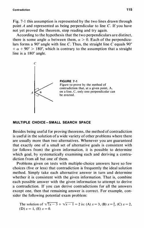
Contradiction 1 1 5

Fig. 7- 1 this assumption is represented by the two l ines drawn through point A and represented as being perpendicular to line C. If you have not yet proved the theorem, stop reading and try again.

According to the hypothesis that the two perpendiculars are distinct, there is some angle a between them, a > O. Each of the perpendicu­lars forms a 90° angle with line C. Thus, the straight l ine C equals 90° + a + 90° > 1 80°, which is contrary to the assumption that a straight l ine is a 1 80° angle .

c

A

FIG U R E 7-1 Figure to prove by the method of contradiction that, at a given point, A, on a l ine , C , only one perpendicular can be erected .

MULTIPLE CHOICE - SMALL SEARCH SPACE

Besides being useful for proving theorems, the method of contradiction is useful in the solution of a wide variety of other problems where there are usual ly more than two alternatives . Whenever you are guaranteed that exactly one of a small set of alternative goals i s consistent with (or follows from) the given information, it is possible to determine which goal , by systematicall y examining each and deriving a contra­diction from all but one of them.

Problems given on tests with multiple-choice answers have so few choices (five or less) that contradiction is frequently the ideal solution method. Simply take each alternative answer in turn and determine whether it is consistent with the given information. That is, combine each possible answer with the given information to attempt to derive a contradiction . If you can derive contradictions for all the answers except one, then that remaining answer i s correct. For example, con­sider the following potential exam problem:

The solution of V7x - 3 + vx=-T = 2 i s : (A) x = 3 , (B) x = � , (C) x = 2 , ( D ) x = I , (E) x = O.

1 1 6 Chapter 7

Stop reading and try to solve this problem, using the method of contradiction .

The slow way to solve the problem is to perform various operations on both sides of the equation (adding, subtracting, multiplying, dividing, squaring both sides of the equation) . The fast way is to substitute each of the alternative values of x into the equation and see which ones work. In this case, only x = 1 is consistent with the equation , so (D) i s the answer.

Solving for the values of one or more variables that satisfy one or more equations is a primary example of problems where often the givens and the goal should be combined. In these problems, there may be several values of a variable, or several sets of values of the several variables , that satisfy the equation or equations . You are being asked to determine one or more such solutions that satisfy the equations, which is in essence saying that consistency of the givens and goal statements is all that is demanded.

When you encounter a problem like this on a multiple-choice test, with a small number of choices for solutions of the equations, then the ideal problem-solving method is contradiction. You simply try each of the alternative solutions in turn to see if it satisfies the equa­tions - that is , gives an answer l ike a = a for all equations - when the set of values of variables is substituted into the equations . All of the incorrect answers will produce contradictions such as 5 = 3. For ex­ample, consider the fol lowing problem:

Which of the fol lowing i s a solution of the cubic equation, X1 + 4x2 - 7x - 1O = O? x equal s : (A) -2, (8) -5, (C) 4, (D) 3 , (E) none of these.

Stop reading and try to solve this problem, using the method of con­tradiction.

In this instance, you can factor the cubic into three l inear factors, yielding three real roots . However, a much faster way to solve the problem is to check each of the first four specific alternative answers for consistency with the cubic equation.

Since one of the answers - namely, x = -5 - is consistent with the cubic equation, and all the rest are not, we know that (8) is the cor­rect answer. Since all you are asked is whether a particular alternative goal is consistent with the given information (the cubic equation), determining one answer that is consistent is sufficient to solve the problem. You need not actually derive contradictions in the case of alternatives (e) and (D) , except as a check that your determination of consistency in the case of alternative (8) was correct. If alternative

Contradiction 1 17

(E) was an expression such as "several of these," it would be neces­sary to derive contradictions to all but one of the first four alterna­tive answers in order to rule out this alternative.

Contradiction is useful in examinations on a very wide variety of problems. For example, consider the following:

The base of our number system i s 1 0. I f the base were changed to four you would count as fol lows: I , 2 , 3 , 1 0, I I , 1 2 , 1 3 , 20, 2 1 , 22 , 2 3 , 30 , and so on. The 22nd number in the base-four system i s : (A) 2 2 , (B ) 37 , (C) 64 , (D) 1 04, (E) 1 1 2 .

Stop reading and try to answer th is question, us ing the method of contradiction.

In a number system with base of four, the digits 4 , 5, 6, 7, 8, and 9 cannot appear. Thus , alternative answers (B) , (C) , and (0) could not possibly be correct. In addition, the number 22 has already been used prior to ach ieving the 22nd number in the base-four system. Thus, the only possible answer of the five that could be correct is answer (E), which is 1 1 2 .

Some problems are necessari ly solved by contradiction. For ex­ample, consider the fol lowing problem:

The formula express ing the relationship between x and y in the table is :

x

y

2 3

2 3 6

4 5

1 1 1 8

(A) y = 2x + I , (B) y = -r + 2x2 + I , (C) y = x' - 2r + 3x2 - x + I , (D) y = x2 - 2x + 3, (E) y = x2 + l .

Stop reading and try to solve this problem, using the method of contradiction .

The correct answer is alternative (0), and there is really no other way to determine that (0) is the correct answer except by using the method of contradiction. Infinitely many different functions are con­sistent with any finite number of points, and infinitely many d ifferent functions are inconsistent with any finite number of points . All we can do is to determine which functions are consistent and which are in­consistent by checking for contradictions between the proposed func­tions (goals) and the given information about points on the function.

No one would object to your using the method of contradiction to solve such problems in an examination s ituation and, of course, to

1 18 Chapter 7

using it in the case of indirect proof. However, I have occasionally heard objections to its being used in some of the above examples of multiple-choice problems, where there are direct methods for deter­mining the goal from the given information. Some teachers have even protested that for students to use the answers and look for contra­dictions is mildly immoral , that it "educates people to be test takers . "

It is true that such students are not demonstrating their knowledge of the direct algorithmic methods for obtaining the goal from the given information. However, I think we must face the fact that these types of test questions simply do not adequately assess a student' s knowledge of algorithmic methods , because the method of contradiction can be used in place of the algorithms. Some students are inevitably going to use the method of contradiction whether anybody tel ls them about it or not, and this only introduces an extra source of noise in the rela­tive assessment of understanding of d ifferent students. Test questions must be made fool-proof; it will not do to ask students to be fools. Furthermore , there are many times when a teacher wants to assess students ' knowledge of certain specific mathematical concepts with questions that can be answered using the method of contradiction , and it is either not possible or the teacher does not care to assess their understanding of any algorithmic method for generating the solution.

Another class of problems that involves a search among a small population of alternative goals are the recreational logic problems that make up such a large part of problem books. In many of these problems it is difficult to make inferences from the givens to the goal , but it is generally quite easy to test any given assumption about the goal for consistency with the given information. Since the number of alternative goals is often quite smal l , the method of contradiction is ideally suited to the solution of such problems. Some of the most interesting recreational logic problems that are the most difficult to solve by inferences from the givens to the goal are problems involv­ing the possibil ity that some of the given information is false. These are the famous liar and truth-tel ler (truar) problems. We discussed one such problem in Chapter 3 in connection with the need for having a c lear understanding of the goal ; let us consider it again here from the standpoint of the method of contradiction :

The country of Marr is inhabited by two types of people, l iars and truars (truth tellers). Liars always lie and truars always tel l the truth. As the newly appointed United States ambassador to Marr, you have been in­v ited to a local cocktail party. While consuming some of the native spirits , you are engaged in conversation with three of Marr's most prominent

Contradiction 1 19

citizens: Joan Landill, Shawn Farrar, and Peter Gant. At one point in the conversation Joan remarks that Shawn and Peter are both l iars. Shawn vehemently denies that he i s a l iar, but Peter replies that Shawn is indeed a l iar. From this information , can you determine how many of the three are l iars and how many are truars?

Stop reading and try to solve this problem, using the method of contradiction. You wil l recall from Chapter 3 that all we need to deter­mine is how many of the three are l iars - namely, whether there are zero, one, two, or three l iars among the three people . However, in order to determine this number, it i s usefu l to consider all eight pos­sibil ities for the l iar-versus-truar status of Joan, Shawn, and Peter­namely, a l l three are l iars ; Joan and Shawn are truars , but Peter is a l iar ; Joan and Peter are l iars , but Shawn i s a truar ; Shawn and Peter are l iars , but Joan is a truar; Joan is a l iar, but Shawn and Peter are truars ; Shawn is a l iar, and Joan and Peter are truars ; and , finally, Peter is a l iar, and Joan and Shawn are truars . It i s easy to test the consistency of each of these eight possibilities with the given informa­tion of each of these eight possibil ities. For example , all three cannot be truars , since Joan would not then say that both Shawn and Peter were l iars. All three cannot be lying, since Peter would not then say that Shawn was a l iar. We can also rule out each of the three possibil i­ties in which there are one l iar and two truars in the group. Of the remaining three possibilities , we can rule out the possibil ity that Joan is a truar and both Shawn and Peter are l iars , but we cannot find a contradiction to either of the other two possibil ities - namely, that Joan and Shawn are l iars and Peter is a truar, or that Joan and Peter are l iars and Shawn is a truar. As discussed in Chapter 3 , the inabi l ity to decide between these two possibil ities is of no consequence to the solution of the original problem, since all we were asked to determine was how many of the three are l iars . Under either of the two possibil ities that are not contradictory with the given information, there are exactly two l iars and one truar, which is the answer to the problem.

Instead of examining all eight combinations of Iiar-and-truar status for each of the three people, it is possible to use the method of con­tradiction somewhat more efficiently by considering various classes of the eight alternatives . For instance, a judicious choice would be to consider the class of possibilities in which Joan is a truar. All of the four members of this class can be shown to be contradictory to the given information , since then both Shawn and Peter must be l iars and Shawn would then be tell ing the truth - a contradiction . This classifica­tory use of the method of contradiction is discussed more extensively in the next section. In problems involving search through only a small

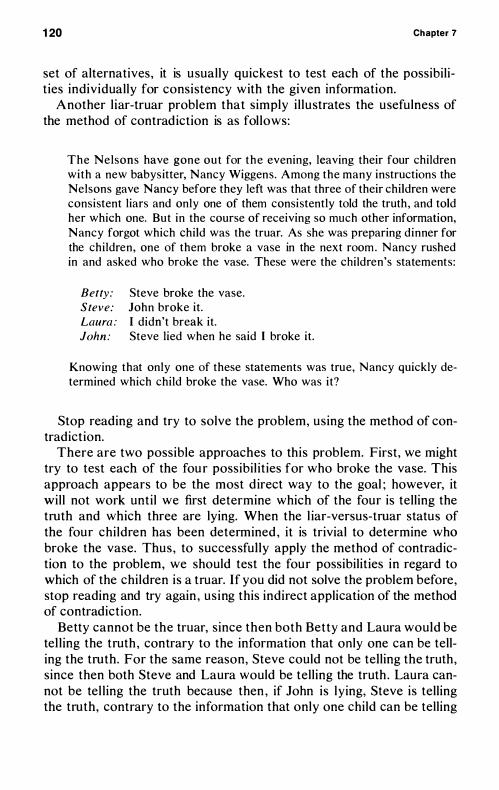
1 20 Chapter 7

set of alternatives, it is usually quickest to test each of the possibili­ties individually for consistency with the given information.

Another l iar-truar problem that simply i l lustrates the usefulness of the method of contradiction is as fol lows:

The Nelsons have gone out for the evening, leaving their four children with a new babysitter, Nancy Wiggens. Among the many instructions the Nelsons gave Nancy before they left was that three of their children were consistent liars and only one of them consistently told the truth, and told her which one. But in the course of receiving so much other information, Nancy forgot which child was the truar. As she was preparing dinner for the children, one of them broke a vase in the next room . Nancy rushed in and asked who broke the vase. These were the children's statements:

Betty: Steve: Laura : John :

Steve broke the vase. John broke it. I didn't break it. Steve lied when he said I broke it.

Knowing that only one of these statements was true, Nancy quickly de­termined which child broke the vase. Who was it?

Stop reading and try to solve the problem, using the method of con­tradiction.

There are two possible approaches to this problem. First, we might try to test each of the four possibil ities for who broke the vase. This approach appears to be the most d irect way to the goal ; however, it wil l not work until we first determine which of the four is telling the truth and which three are lying. When the l iar-versus-truar status of the four chi ldren has been determined , it is trivial to determine who broke the vase. Thus , to successfully apply the method of contradic­tion to the problem, we should test the four possibilities in regard to which of the children is a truar. If you did not solve the problem before, stop reading and try again , us ing this indirect application of the method of contradiction.

Betty cannot be the truar, since then both Betty and Laura would be tel l ing the truth , contrary to the information that only one can be tell­ing the truth. For the same reason, Steve could not be telling the truth , since then both Steve and Laura would be telling the truth . Laura can­not be tel l ing the truth because then , if John is lying, Steve is telling the truth, contrary to the information that only one child can be telling

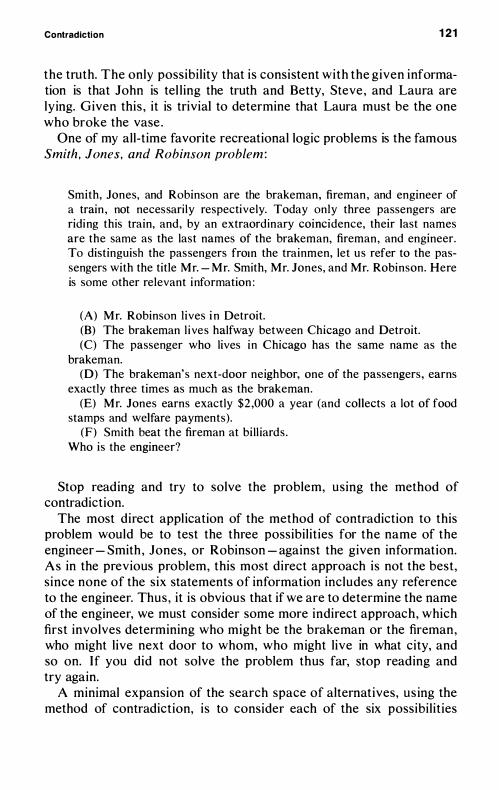
Contradiction 121

the truth. The only possibility that is consistent with the given informa­tion is that John is tel l ing the truth and Betty, Steve , and Laura are lying. Given this , it is trivial to determine that Laura must be the one who broke the vase .

One of my all-time favorite recreational logic problems is the famous Smith , Jones, and Robinson problem :

Smith, Jones, and Robinson are the brakeman, fireman , and engineer of a train , not necessari ly respectively. Today only three passengers are riding this train, and, by an extraordinary coincidence, their last names are the same as the last names of the brakeman, fireman, and engineer. To distinguish the passengers from the trainmen, let us refer to the pas­sengers with the title Mr. - Mr. Smith, Mr. Jones, and Mr. Robinson. Here is some other relevant information :

(A) Mr. Robinson lives i n Detroit. (B) The brakeman l i ves halfway between Chicago and Detroit. (C) The passenger who lives in Chicago has the same name as the

brakeman. (D) The brakeman's next-door neighbor, one of the passengers , earns

exactly three times as much as the brakeman. (E) Mr. Jones earns exactly $2 ,000 a year (and collects a lot of food

stamps and welfare payments). (F) Smith beat the fireman at bil l iards .

Who is the engineer?

Stop reading and try to solve the problem, using the method of contradiction.

The most direct appl ication of the method of contradiction to this problem would be to test the three possibil ities for the name of the engineer - Smith , Jones, or Robinson - against the given information. As in the previous problem, this most direct approach is not the best, since none of the six statements of information includes any reference to the engineer. Thus , it is obvious that if we are to determine the name of the engineer, we must consider some more indirect approach, which first involves determining who might be the brakeman or the fireman, who might live next door to whom, who might live in what city, and so on. If you did not solve the problem thus far, stop reading and try again.

A minimal expansion of the search space of alternatives, us ing the method of contradiction, is to consider each of the six possibil ities

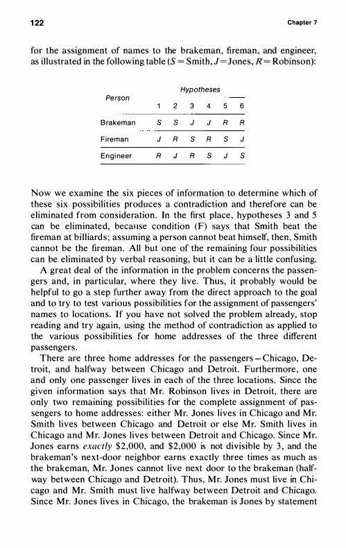
1 22 Chapter 7

for the assignment of names to the brakeman , fireman, and engineer, as i l lustrated in the fol lowing table (S = Smith , J =Jones, R = Robinson):

Person

B rakeman

F i reman

Eng i neer

Hypotheses

2 3 4 5 6

S S J J R R

J R S R S J

R J R S J S

Now we examine the six pieces of information to determine which of these six possibil ities produces a contradiction and therefore can be eliminated from consideration . In the first place , hypotheses 3 and 5 can be el iminated, because condition (F) says that Smith beat the fireman at bi l l iard s ; assuming a person cannot beat himself, then , Smith cannot be the fireman. All but one of the remaining four possibilities can be eliminated by verbal reasoning, but it can be a little confusing.

A great deal of the information in the problem concerns the passen­gers and, in particular, where they live. Thus , it probably would be helpful to go a step further away from the direct approach to the goal and to try to test various possibilities for the assignment of passengers' names to locations. If you have not solved the problem already, stop reading and try again, using the method of contradiction as applied to the various possibil ities for home addresses of the three d ifferent passengers .

There are three home addresses for the passengers - Chicago, De­troit, and halfway between Chicago and Detroit. Furthermore , one and only one passenger l ives in each of the three locations. Since the given information says that Mr. Robinson l ives in Detroit, there are only two remaining possibil ities for the complete assignment of pas­sengers to home addresses : e ither Mr. Jones l ives in Chicago and Mr. Smith l ives between Chicago and Detroit or else Mr. Smith l ives in Chicago and Mr. Jones l ives between Detroit and Chicago. Since Mr. Jones earns exactly $2 ,000, and $2 ,000 is not divisible by 3 , and the brakeman's next-door neighbor earns exactly three times as much as the brakeman, Mr. Jones cannot l ive next door to the brakeman (half­way between Chicago and Detroit). Thus , Mr. Jones must live in Chi­cago and Mr. Smith must l ive halfway between Detroit and Chicago. Since Mr. Jones l ives in Chicago, the brakeman is Jones by statement

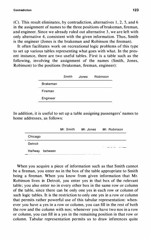
Contradiction 123

(e) . This result eliminates , by contradiction, alternatives 1 , 2 , 5, and 6 in the assignment of names to the three positions of brakeman, fireman, and engineer. Since we already ruled out alternative 3 , we are left with only alternative 4, consistent with the given information. Thus , Smith is the engineer (Jones is the brakeman and Robinson the fireman) .

It often facil itates work on recreational logic problems of this type to set up various tables representing what goes with what. In the pres­ent instance, there are two useful tables. First is a table such as the fol lowing, involving the assignment of the names (Smith , Jones, Robinson) to the positions (brakeman, fireman, engineer) :

Brakeman

F i reman

Eng ineer

Smith Jones Robinson

In addition , it is useful to set up a table assigning passengers' names to home addresses, as follows :

Mr. Smith Mr. Jones Mr. Robinson

Ch icago

Detro it

Ha l fway between

When you acquire a piece of information such as that Smith cannot be a fireman, you enter no in the box of the table appropriate to Smith being a fireman. When you know from given information that Mr. Robinson l ives in Detroit, you enter yes in that box of the relevant table ; you also enter no in every other box in the same row or column of the table, since there can be only one yes in each row or column of such logic tables. It is the restriction to only one yes in a row or column that permits rather powerful use of this tabular representation : when­ever you have a yes in a row or column, you can fill in the rest of both the row and the column with nos ; whenever you have two nos in a row or column, you can fill in a yes in the remaining position in that row or column. Tabular representation permits us to draw inferences quite

1 24 Chapter 7

mechanically from previous inferences that are recorded in the table, avoiding complicated verbal reasoning and the possibility of memory loss . The finished versions of these two tables for solution of this Smith , Jones, Robinson problem are shown in Fig. 7-2.

Smith Jones Robinson

Brakeman No Yes No

F i reman No No Yes

Eng i neer Yes No No

Mr. Sm ith Mr. Jones Mr. Robinson

C h i cag o N o Yes No

Detro it N o N o Yes

Between Yes N o No

R G U R E 7-2 Final tables for solution of Smith, Jones , and Robinson problem.

A final problem of a completely different kind that il lustrates the usefulness of the method of contradiction is a spatial-puzzle problem that I have called the bowling-pin reversal problem:

Six-year-old Heather Phillips set up the ten p ins for her bowling game at the end of the hall in a manner exactly opposite to the correct configura­tion. Before Heather could throw the bowling ball down the hall, her father informed her that she had set up the pins in the wrong manner and that the pins should have the row of one pin in front, followed by the row of two pins, followed by the row of three, and , finally, the row of four in the back. Although Heather is given to childish reversal errors of this type when she forgets to put on her thinking cap, she is actually a budding mathematical genius . So, upon being informed of her error, Heather quickly put her thinking cap back on, ran down the hall, and , by moving just three pins, was able to reverse the configuration from the given state to the goal state , as illustrated in Fig. 7-3 . How did she do it? (By the way, Heather assumed that the exact placement of the pins on the floor was not important, so long as the relative placement of the pins with respect to each other was correct. You should assume this also.)

Stop reading, put on your thinking cap (if you do not have it on al­ready), and try to solve the problem, using the method of contradiction (not just random trial and error) .

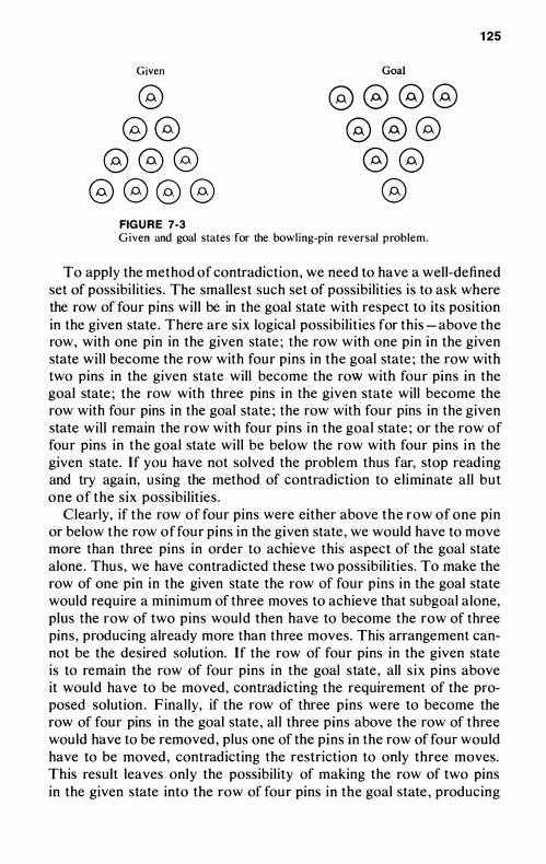
Given

@ @ @

@ @ @ @ @ @ @

FIG U R E 7-3

Goal

@ @ @ @ @ @ @

@ @ @

Given and goal states for the bowling-pin reversal problem.

125

To apply the method of contradiction , we need to have a well-defined set of possibi lities . The smallest such set of possibilities is to ask where the row of four pins wil l be in the goal state with respect to its position in the given state . There are six logical possibil ities for this - above the row, with one pin in the given state ; the row with one pin in the given state wil l become the row with four pins in the goal state ; the row with two pins in the given state will become the row with four pins in the goal state ; the row with three pins in the given state will become the row with four pins in the goal state ; the row with four pins in the given state wil l remain the row with four pins in the goal state ; or the row of four pins in the goal state wil l be below the row with four pins in the given state . If you have not solved the problem thus far, stop reading and try again, using the method of contradiction to el iminate all but one of the six possibilities .

Clearly, if the row of four pins were either above the row of one pin or below the row of four pins in the given state , we would have to move more than three pins in order to achieve this aspect of the goal state alone . Thus, we have contradicted these two possibilities. To make the row of one pin in the given state the row of four pins in the goal state would require a minimum of three moves to achieve that subgoal alone, plus the row of two pins would then have to become the row of three pins, producing already more than three moves. This arrangement can­not be the desired solution. If the row of four pins in the given state is to remain the row of four pins in the goal state , all s ix pins above it would have to be moved, contrad icting the requirement of the pro­posed solution . Finally, if the row of three pins were to become the row of four pins in the goal state , al l three pins above the row of three would have to be removed , plus one of the pins in the row of four would have to be moved , contradicting the restriction to only three moves. This result leaves only the possibility of making the row of two pins in the given state into the row of four pins in the goal state , producing

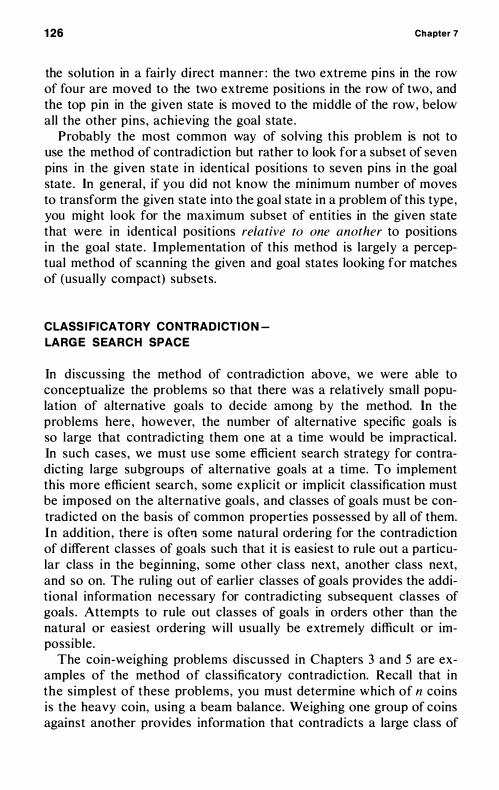
126 Chapter 7

the solution in a fairly direct manner : the two extreme pins in the row of four are moved to the two extreme positions in the row of two, and the top pin in the given state is moved to the middle of the row, below all the other pins, achieving the goal state .

Probably the most common way of solving this problem is not to use the method of contradiction but rather to look for a subset of seven pins in the given state in identical positions to seven pins in the goal state . In general , if you did not know the minimum number of moves to transform the given state into the goal state in a problem of this type , you might look for the maximum subset of entities in the given state that were in identical positions relative to one another to positions in the goal state . Implementation of this method is largely a percep­tual method of scanning the given and goal states looking for matches of (usually compact) subsets.

CLASSIFICATORY CONTRADICTION ­

LARGE SEARCH SPACE

In discussing the method of contradiction above, we were able to conceptualize the problems so that there was a relatively small popu­lation of alternative goals to decide among by the method. In the problems here , however, the number of alternative specific goals is so large that contradicting them one at a time would be impractical . In such cases , we must use some efficient search strategy for contra­dicting large subgroups of alternative goals at a time. To implement this more efficient search, some explicit or implicit classification must be imposed on the alternative goal s , and classes of goals must be con­tradicted on the basis of common properties possessed by all of them. In add ition , there i s oftell some natural ordering for the contradiction of d ifferent classes of goals such that it is easiest to rule out a particu­lar class in the beginning, some other class next, another class next, and so on. The rul ing out of earlier classes of goals provides the addi­tional information necessary for contradicting subsequent classes of goals . Attempts to rule out classes of goals in orders other than the natural or easiest ordering wil l usually be extremely difficult or im­possible.

The coin-weighing problems discussed in Chapters 3 and 5 are ex­amples of the method of classificatory contradiction. Recall that in the simplest of these problems, you must determine which of n coins is the heavy coin, using a beam balance. Weighing one group of coins against another provides information that contradicts a large class of

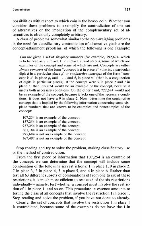
Contradiction 1 27

possibilities with respect to which coin is the heavy coin. Whether you consider these problems to exemplify the contradiction of one set of alternatives or the implication of the complementary set of al­ternatives is obviously completely arbitrary.

A class of problems somewhat similar to the coin-weighing problems in the need for classificatory contradiction of alternative goals are the concept-attainment problems, of which the fol lowing is one example:

You are given a set of six-place numbers (for example , 792 ,674, which is to be read as 7 in place I , 9 in place 2 , and so on), some of which are examples of the concept and some of which are not. Concepts are either simple concepts of the form "concept is d in place p" (that i s , a particular digit d in a particular place p) or conjunctive concepts of the form "con­cept is dl in place P I and . . . and di in place p;" (that is , a conjunction of digits in particular places). If the concept were 9 in place 2 and 7 in place 5 , then 792,674 would be an example of the concept, because it meets both necessary conditions. On the other hand , 722 ,674 would not be an example of the concept, because it lacks one of the necessary condi­tions: it does not have a 9 in place 2 . Now, determine the conjunctive concept that is implied by the following information concerning some six­place numbers that are known to be examples and nonexamples of the concept:

1 07 ,254 is an example of the concept. 1 57 ,254 is an example of the concept. 937 ,254 is an example of the concept. 867, 1 84 is an example of the concept. 295,684 is not an example of the concept. 367 ,497 is not an example of the concept.

Stop reading and try to solve the problem, making classificatory use of the method of contradiction.

From the first piece of information that 1 07 ,254 is an example of the concept, we can determine that the concept wil l include some combination of the fol lowing six restrictions : 1 in place 1 , 0 in place 2 , 7 in place 3 , 2 in place 4, 5 i n place 5 , and 4 in place 6. Rather than test all 63 different subsets of combinations of from one to six of these restrictions, it is much more efficient to test each of the six restrictions individual ly - namely, test whether a concept must involve the restric­tion of 1 in place 1 , and so on. This procedure in essence amounts to testing the class of all concepts that involve the restriction 1 in place 1 . Stop reading and solve the problem, if you have not done so already.

Clearly, the set of concepts that involve the restriction I in place 1 is contradicted , because some of the examples do not have the 1 in

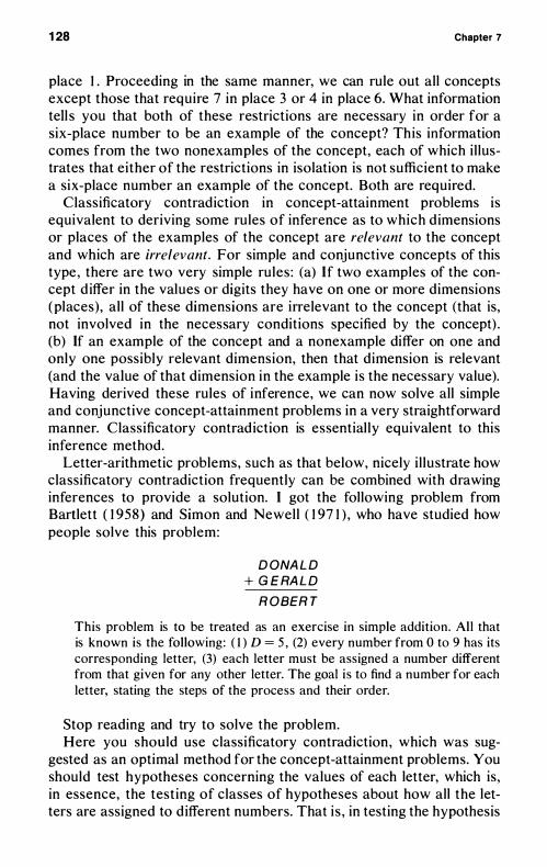
1 28 Chapter 7

place 1 . Proceeding in the same manner, we can rule out all concepts except those that require 7 in place 3 or 4 in place 6. What information tell s you that both of these restrictions are necessary in order for a six-place number to be an example of the concept? This information comes from the two nonexamples of the concept, each of which i l lus­trates that either of the restrictions in isolation is not sufficient to make a six-place number an example of the concept. Both are required.

Classificatory contradiction in concept-attainment problems is equivalent to deriving some rules of inference as to which d imensions or places of the examples of the concept are relevant to the concept and which are irrelevant. For simple and conjunctive concepts of this type , there are two very simple rules : (a) If two examples of the con­cept d iffer in the values or digits they have on one or more dimensions (places), all of these dimensions are irrelevant to the concept (that is, not involved in the necessary conditions specified by the concept) . (b) If an example of the concept and a nonexample differ on one and only one possibly relevant dimension, then that dimension is relevant (and the value of that dimension in the example is the necessary value). Having derived these rules of inference, we can now solve all simple and conjunctive concept-attainment problems in a very straightforward manner. Classificatory contradiction is essential ly equivalent to this inference method.

Letter-arithmetic problems, such as that below, nicely i l lustrate how classificatory contradiction frequently can be combined with drawing inferences to provide a solution. I got the following problem from Bartlett ( 1 958) and Simon and Newell ( 1 97 1 ) , who have studied how people solve this problem:

D ONA L D + G E RA L D

R O BER T This problem is to be treated as an exercise in simple addition. All that is known is the following : ( I ) D = 5 , (2) every number from 0 to 9 has its corresponding letter, (3) each letter must be assigned a number different from that given for any other letter. The goal is to find a number for each letter, stating the steps of the process and their order.

Stop reading and try to solve the problem. Here you should use classificatory contradiction , which was sug­

gested as an optimal method for the concept-attainment problems. You should test hypotheses concerning the values of each letter, which is, in essence, the testing of classes of hypotheses about how all the let­ters are assigned to d ifferent numbers. That i s , in testing the hypothesis

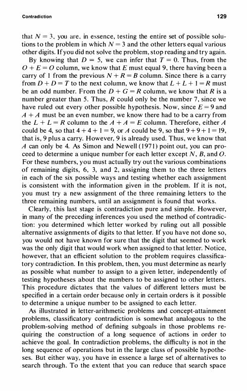
Contradiction 1 29

that N = 3 , you are , in essence, testing the entire set of possible solu ­tions to the problem in which N = 3 and the other letters equal various other digits. If you did not solve the problem, stop reading and try agai n.

By knowing that D = 5, we can infer that T = O. Thus, from the o + E = 0 column, we know that E must equal 9 , there having been a carry of 1 from the previous N + R = B column. Since there is a carry from D + D = T to the next column, we know that L + L + 1 = R must be an odd number. From the D + G = R column, we know that R is a number greater than 5 . Thus , R could only be the number 7 , since we have ruled out every other possible hypothesis . Now, since E = 9 and A + A must be an even number, we know there had to be a carry from the L + L = R column to the A + A = E column. Therefore , either A could be 4, so that 4 + 4 + 1 = 9, or A could be 9 , so that 9 + 9 + 1 = 19 , that i s , 9 p lus a carry. H owever, 9 i s already used. Thus , we know that A can only be 4. As Simon and Newell ( 1 97 1 ) point out, you can pro­ceed to determine a unique number for each letter except N, B, and O. For these numbers, you must actually try out the various combinations of remaining digits, 6 , 3, and 2 , assigning them to the three letters in each of the six possible ways and testing whether each assignment is consistent with the information given in the problem. If it is not, you must try a new assignment of the three remaining letters to the three remaining numbers, until an assignment is found that works .

C learly, this last stage is contradiction pure and simple. However, in many of the preceding inferences you used the method of contradic­tion : you determined which letter worked by ruling out all possible alternative assignments of digits to that letter. If you have not done so, you would not have known for sure that the d igit that seemed to work was the only digit that would work when assigned to that letter. Notice, however, that an efficient solution to the problem requires classifica­tory contradiction. In this problem, then, you must determine as nearly as possible what number to assign to a given letter, independently of testing hypotheses about the numbers to be assigned to other letters . This procedure dictates that the values of d ifferent letters must be specified in a certain order because only in certain orders is it possible to determine a unique number to be assigned to each letter.

As il lustrated in letter-arithmetic problems and concept-attainment problems, classificatory contradiction is somewhat analogous to the problem-solving method of defining subgoals in those problems re­quiring the construction of a long sequence of actions in order to achieve the goal . In contradiction problems, the difficulty is not in the long sequence of operations but in the large class of possible hypothe­ses. But either way, you have in essence a large set of alternatives to search through . To the extent that you can reduce that search space

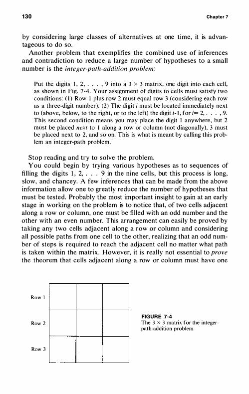
130 Chapter 7

by considering large classes of alternatives at one time, it is advan­tageous to do so.

Another problem that exemplifies the combined use of inferences and contradiction to reduce a large number of hypotheses to a small number is the integer-path-addition problem :

Put the digits I , 2 , . . . , 9 into a 3 X 3 matrix, one d igit into each cell, as shown in Fig. 7-4. Your assignment of digits to cells must satisfy two conditions : ( I ) Row I plus row 2 must equal row 3 (considering each row as a three-digit number). (2) The digit i must be located immediately next to (above, below, to the right, or to the left) the digit i- I , for i= 2, . . . , 9 . This second condition means you may place the digit I anywhere , but 2 must be placed next to I along a row or column (not diagonally), 3 must be placed next to 2, and so on. This is what is meant by calling this prob­lem an integer-path problem.

Stop reading and try to solve the problem. You could begin by trying various hypotheses as to sequences of

fil l ing the digits I , 2, . . . 9 in the nine cel l s , but this process is long, slow, and chancey. A few inferences that can be made from the above information allow one to greatly reduce the number of hypotheses that must be tested. Probably the most important insight to gain at an early stage in working on the problem is to notice that, of two cells adjacent along a row or column, one must be fil led with an odd number and the other with an even number. This arrangement can easily be proved by taking any two cells adjacent along a row or column and considering all possible paths from one cell to the other, real izing that an odd num­ber of steps is required to reach the adjacent cell no matter what path is taken within the matrix . However, it is real ly not essential to prove the theorem that cel ls adjacent along a row or column must have one

Row I

Row 2

Row 3

FIG U R E 7-4 The 3 x 3 matrix for the integer­path-addition problem.

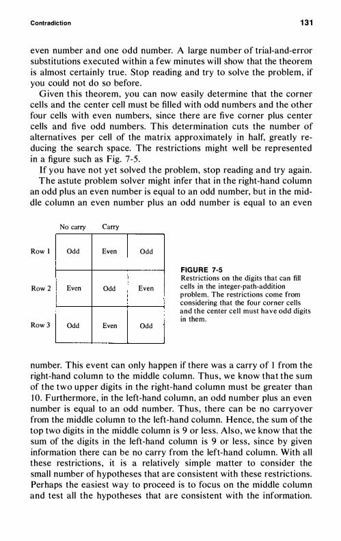
Contradiction 131

even number and one odd number. A large number of trial-and-error substitutions executed within a few minutes wil l show that the theorem is almost certainly true. Stop reading and try to solve the problem, if you could not do so before .

Given th is theorem, you can now easily determine that the corner cel ls and the center cell must be filled with odd numbers and the other four cells with even numbers, since there are five corner plus center cells and five odd numbers. This determination cuts the number of alternatives per cell of the matrix approximately in half, greatly re­ducing the search space. The restrictions might well be represented in a figure such as Fig. 7-5 .

If you have not yet solved the problem, stop reading and try again. The astute problem solver might infer that in the right-hand column

an odd plus an even number i s equal to an odd number, but in the mid­dle column an even number plus an odd number is equal to an even

Row I

Row 2

Row 3

No carry Carry

Odd Even

Even Odd

Odd Even

Odd

Even

Odd

FIG U R E 7-5 Restrictions on the digits that can fill cel ls in the integer-path-addition problem. The restrictions come from considering that the four corner cel ls and the center cel l must have odd digits in them.

number. This event can only happen if there was a carry of I from the right-hand column to the middle column. Thus , we know that the sum of the two upper digits in the right-hand column must be greater than 1 0 . Furthermore , in the left-hand column, an odd number plus an even number is equal to an odd number. Thus , there can be no carryover from the middle column to the left-hand column. Hence, the sum of the top two digits in the middle column is 9 or less . Also, we know that the sum of the digits in the left-hand column is 9 or less , since by given information there can be no carry from the left-hand column. With all these restrictions , it i s a relatively simple matter to consider the small number of hypotheses that are consistent with these restrictions. Perhaps the easiest way to proceed is to focus on the middle column and test all the hypotheses that are consistent with the information.

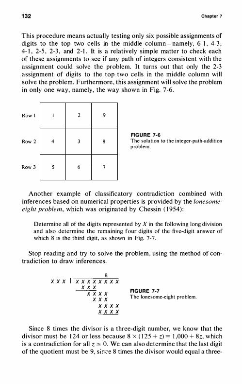
1 32 Chapter 7

This procedure means actually testing only six possible assignments of digits to the top two cel ls in the middle column - namely, 6- 1 , 4-3 , 4- 1 , 2-5 , 2-3 , and 2- 1 . It is a relatively simple matter to check each of these assignments to see if any path of integers consistent with the assignment could solve the problem. It turns out that only the 2-3 assignment of d igits to the top two cel ls in the middle column will solve the problem. Furthermore , this assignment wil l solve the problem in only one way, namely, the way shown in Fig. 7-6 .

Row I I 2

Row 2 4 3

Row 3 5 6

9

8

7

FIG U R E 7-6 The solution to the integer-path-addition problem.

Another example of classificatory contradiction combined with inferences based on numerical properties is provided by the lonesome­eight problem, which was originated by Chessin ( 1 954) :

Determine all of the d igits represented by X in the following long division and also determine the remaining four digits of the five-d igit answer of which 8 is the third digit, as shown in Fig. 7-7 .

Stop reading and try to solve the problem, using the method of con­tradiction to draw inferences.

8

x x x X X X X X X X X X X X

X X X X X X X

X X X X X X X X

R G U R E 7-7 The lonesome-eight problem.

Since 8 times the divisor i s a three-digit number, we know that the divisor must be 1 24 or less because 8 x ( 1 25 + z) = 1 ,000 + 8z, which is a contradiction for all z � o. We can also determine that the last digit of the quotient must be 9, si:-;;:e 8 times the divisor would equal a three-

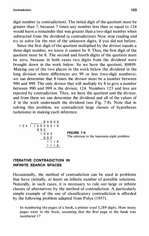
Contradiction 133

digit number (a contradiction) . The initial digit of the quotient must be greater than 7, because 7 times any number less than or equal to 1 24 would leave a remainder that was greater than a two-digit number when subtracted from the dividend (a contradiction). Now stop reading and try to solve for the rest of the unknown digits , if you did not before .

Since the first digit of the quotient multiplied by the d ivisor equal s a three-digit number, we know it cannot be 9. Thus, the first digit of the quotient must be 8 . The second and fourth digits of the quotient must be zero, because in both cases two digits from the dividend were brought down in the work below. So we have the quotient, 80809. Making u se of the two places in the work below the dividend in the long division where differences are 99 or less (two-digit numbers) , we can determine that 8 times the divisor must be a number between 990 and 999. The only divisor that will multiply by 8 to give a number between 990 and 999 is the divisor, 1 24. Numbers 1 23 and less are rejected by contradiction. Thus , we have the quotient and the divisor, and from them we can determine the dividend and all of the values of X in the work underneath the d ividend (see Fig. 7-8) . Note that in solving this problem, we contradicted large classes of hypotheses (solutions) in making each inference.

8 0 8 0 9

1 2 4 1 0 0 2 0 3 1 6

9 9 2

1 0 0 3

9 9 2

1 1 1 6

1 1 1 6

FIG U R E 7-8 The solution to the lonesome-eight problem.

ITERATIVE CONTRADICTION IN

INFINITE SEARCH SPACES

Occasionally, the method of contradiction can be used in problems that have (initial ly, at least) an infinite number of possible solutions. Natural ly, in such cases, it i s necessary to rule out large or infinite classes of alternatives by the method of contradiction . A particularly simple example of the use of classificatory contradiction is afforded by the following problem adapted from Polya ( 1 957) .

In numbering the pages of a book, a printer used 3 ,289 digits . H ow many pages were in the book, assuming that the first page in the book was numbered I ?

134 Chapter 7

Stop reading and try to solve the problem, using the method of clas­sificatory contradiction to ru le out all but one of the infinity of positive integer answers.

Of course, there are not an infinite number of solutions to the prob­lem, once one draws a relatively trivial inference. The inference is that the number of pages cannot possibly be greater than the number of digits (3 ,289) , since at least one d igit has to be used to number each page . Thus , we might well regard this problem as an example of clas­sificatory contradiction in a large , but finite, search space. However, since an inference using the method of contradiction was necessary in order to make the search space finite, it seems appropriate to con­sider the problem as having an initial ly infinite search space.

The problem provides a particularly simple example of the use of the iterative method of taking a preliminary estimate of the goal , determining the magnitude of the error of the estimate from the goal , then moving in the direction of the goal to obtain another estimate along with a magnitude of error, and so on, hoping ultimately to con­verge upon the goal . S ince the preliminary estimates are contradicted by the given information, I think it is useful to consider iterative methods as a subclass of the method of contradiction, a subclass that is particularly usefu l in solving problems with infinite (but ordered) search spaces. Now stop reading, and try again to solve the problem, if you could not before.

To make the iterative solution to this problem clear, imagine that we start with a preliminary estimate of nine pages for the book. Each page is a single d igit. Thus , nine digits in all would be used to number the book. This number is clearly too l ittle , so we move up to the end of the two-digit numbers, namely, the number 99. Numbering 99 pages requires 9 single digits plus 90 two-digit numbers , for a total of 9 + 1 80 , or 1 89 d igits. The number 1 89 is st i l l substantially below the number 3 ,289 . Thus , for our next estimate we will take the end of the three­digit numbers, namely, 999. N umbering 999 pages uses nine single­digit numbers plus 90 two-digit numbers plus 900 three-digit numbers , for a total of 9 + 1 80 + 2700, or 2 ,889 digits. This figure is quite close to the target of 3 ,289 digits , so we are encouraged perhaps to try a more direct analytic method at this point, namely, subtracting 2,889 from 3 ,289 to obtain an additional 400 digits that are needed to achieve the goal . (However, note that one could continue to use the iterative method . ) Since we are now in the four-digit numbers, each page will require four digits. Thus, to use 400 more d igits will require 1 00 ad­ditional pages . Thus , we can infer that we must add 1 00 to 999 to ob­tain an answer of 1 ,099 pages in the book , in order to use up 3 ,289 digits.

Contradiction 135

Iterative methods are frequently used in the numerical solution for roots of equations. For example, consider the fol lowing problem:

Determine the roots ( permissible values of x) that satisfy the equation x6 - 4.x" + 2x" + 3.il - 7 x2 + 1 3x - 30 = O.

Stop reading and attempt to specify an iterative method of contra­diction, by which one might determine each root (permissible value of x) for the preceding equation. You can assume that you have a com­puter at your disposal to carry out the large number of steps that might be required in order to converge upon each real solution for this equation.

For large enough positive or negative values of x, the x6 term in the expression must dominate the rest of the expression (be greater than the sum of all the other terms in the expression). Thus , for sufficiently large positive or negative values of x, the expression x6 - 4x" + 2x4 + 3x3 - 7x2 + l 3x - 30 must be greater than zero and monotonical ly in­creasing for more extreme posit ive or negative values of x. Thus , there can be no real solutions for values of x more extreme than these points at which the expression x6 - 4x5 + 2X4 + 3x3 - 7x2 + 1 3x - 30 begins from a positive value monotonical ly to increase without limit. You can either determine these points or else you can make a safe guess , based on the values of the coefficients of the terms in the expression. In this case, you might assume the function to be monotonically increasing above zero for values of x greater than 1 ,000 or less than - 1 ,000. As­suming that the function is monotonically increasing from positive val­ues beyond this range (- 1 ,000 :s x :s + 1 ,000) , we know that there can be no zero crossings (roots) beyond the interval from - 1 ,000 :s x :s + 1 ,000. Thus , by contradiction, we have ru led out all values of x greater than 1 ,000 or less than - 1 ,000. In the present case , we have not done this in a careful way, but we could. Now stop reading and try to solve the problem again , if you failed to sketch an iterative solution method before .

To determine solutions for x within the interval from x = - 1 ,000 to x = + 1 ,000, you may define a step size such that you think it unlikely that there would be two different solutions within a single step. In the present instance, we might choose a step size of unity, though if we wish to be more carefu l we might p ick steps of less than unity. Now we can evaluate the function x5 - 4x5 + 2x4 + 3x3 - 7x2 + 1 3x - 30 at all integer values of x from - 1 ,000 to + 1 ,000 to see if the value of the function changes sides (goes from minus to plus or plus to minus) over the step. If the function does change signs , we know that there

1 36 Chapter 7

is a solution (zero crossing) within the interval defined by that step. We can then proceed to use essential ly the same method (but more efficiently dividing the remaining interval in half each time) to deter­mine the value of the solution to as fine a degree of approximation as we wish. If the function does not change sign over a step, we assume that there is no solution within that interval .

This numerical method for solving higher order equations is called the half-interval search technique and is an excellent example of the iterative use of the method of contradiction . The half-interval search technique uses contradiction, because we consider all intervals over which the function does not change sign not to contain a solution to the equation, since a solution involves a zero crossing (passage from a plus value of the function to a minus value of the function) . The ab­sence of a change from plus to minus over some interval contradicts the possibil ity of a solution in that interval , provided we are justified in assuming that the function cannot have two zero crossings over that interval . If there were some reason to doubt the validity of this for the chosen step size, you could always choose a smaller step size to see if more real roots would be discovered, using the smaller step size. Naturally, if you already found n real roots for an equation of degree n, then you know you have obtained all the roots that it is possible to obtain, since there are at most n real roots for an equation of degree n .

Obviously, the same iterative method can be used to solve other types of equations involving logs, exponents, trig functions, and the l ike. In addition, you can define multidimensional analogs of the above iterative method to solve sets of several equations with several un­knowns. However, it clearly gets more and more time consuming and more and more complicated, the greater the number of unknowns or the more complex the functions.

8

Working Backward

THEORY

The method of working backward is similar to the method of contra­diction (Chapter 7) and the method of drawing inferences about the goal (Chapter 3) in that all three focus on the goal to a great extent and consider it rather than the givens as the starting point for the problem-solving process. However, working backward d iffers in the way the goal is considered in relation to the givens . With the methods of contradiction and drawing inferences from the goal , the goal i s considered to be part of the given information, and we attempt to derive consequences from the goal in conjunction with the givens. Thus, the direction of inference is from the goal statement to some new statements. In working backward, the goal is not considered to be a piece of given information. We start with the goal , but instead of draw­ing inferences from it, we try to guess a preceding statement or state­ments that, taken together, would imply the goal statement. Hence, the direction of inference is the same as in working forward - namely, from the given information to the goal. We start at the end point and

138 Chapter 8

try to determine preceding statements, which need not necessari ly be given statements but which , when taken together, wil l produce the goal . Then we try to determine other statements that will imply those statements, gradually working our way back. We hope to arrive at given information that is sufficient to derive everything in between the givens and the goal .

Why should we want to reverse direction l ike this, proceeding from the goal to the givens rather than from the givens to the goal? When is this method more appropriate than working forward , and why? That is , which problems are appropriate for working backward and which for working forward ?

The method of working backward is l ikely to be useful if a problem satisfies two criteria. The first is that the problem should have a uniquely specified goal, as is the case for all proof problems. When­ever there is a single, c learly, and completely specified goal stated in the problem, you should seriously consider the possibil ity of working backward. This approach is particularly true if, in contrast to the single goal statement, there are large numbers of given statements. Newell , Shaw, and Simon ( 1 962) have clearly stated the advantage to working backward in such problems - namely, there is no ambiguity as to what statement to start with when you work backward , whereas such am­biguity is considerable when you work forward . As they so aptly put it, working forward in such a problem is analogous to finding a needle in a haystack, whereas working backward is analogous to the needle finding its way out of the haystack. You can start from many places outside the haystack in trying to find the single location of the needle. By contrast, the needle starting in a single location can solve the problem of getting out of the haystack by getting to an extremely large number of alternative locations outside the haystack.

In the needle-in-the-haystack problem, the large number of givens have a disjunctive relationship to one another. That is, to solve the problem, you need to get from any one of these givens to the goal or by the method of working backward from the goal to any one of the large number of d ifferent givens . In many problems to which the method of working backward is appropriate, such as proof problems, the givens have a conjunctive relationship to one another. That is, you must use several of the givens to derive the goal . Thus , in the method of working backward, it wil l usually be necessary to work backward from the goal to get to several of the givens rather than to only one of the givens. Nevertheless, the method is frequently very useful in such problems, because the unique starting point so fre-

Working Backward 1 39

quently directs you to just those aspects of the given information that are relevant to the solution.

In problems where the goal i s not so c learly and completely specified and there are , in fact, a variety of possible alternative goals, the ad­vantages of working backward are often largely el iminated. In the case of inference problems (problems with nondestructive operations) , the method of working backward is suitable for proof problems but not generally for find problems. I n the case of action problems (problems with destructive operations) , essential ly the same distinction appl ies ­namely, problems with uniquely specified goals are appropriate for the method of working backward and problems in which only certain characteristics of the goal are specified are general ly not so suitable.

The second criterion of a problem as to whether the method of working backward is applicable concerns the nature of the operations specified in the problem. If all operations are unary and one-to-one operations, the method of working backward i s l ikely to be helpful . U nary operations are operations that take one given input statement and produce one output statement. One-to-one operations are opera­tions for which it is possible to uniquely determine what input state­ments produce the output statement. (These concepts wil l be discussed in more detail in Chapter 1 0. ) Since a well-defined unary operation yields a unique output statement for each input statement, there is no ambiguity concerning the result of an operation when applied to some state working forward . However, a well-defined unary operation need not be one-to-one ; several different input statements could pro­duce the same output statement. Thus , when operations are not one­to-one, working backward may lead to a more rapidly branching tree of possible action sequences than wil l working forward . I n such cases , it would generally be preferable to work forward .

The unary property of an operation is not as important as the one­to-one property for the applicability of working backward . B inary or ternary operations take two or three input statements and produce one output statement. U sing the method of working backward , it would be necessary, given the output statement, to produce two or three input statements . Superficially, this might seem similar to what happens using the method of working backward when operations are not one-to-one. However, there is an important difference - with binary or ternary operations, the inference process is essentially as compli­cated when working forward as when working backward . A conjunc­tion of inputs is related to a single output statement with binary or ternary operations , and this i s equally true working forward or back-

140 Chapter 8

ward. From one problem to another, it may be more or less difficult to work in the forward or the backward direction , but the existence of b inary or ternary operations does not necessari ly invalidate work­ing backward , and examples of working backward in just such problems wil l be given later in the chapter. In such problems, working backward general ly results in a set of subgoal statements , and then the subgoal statements are frequently derived from the givens by working either forward or backward .

By contrast, with operations that are not one-to-one , working back­ward generates a multiplicity of alternative input statements that are disjunctively related one to another (rather than conjunctively related) . Thus , you are generating a large set of alternative prior statements, using the method of working backward , which would never be present using the method of working forward , since only one of these state­ments is necessary in order to derive the goal (not a conjunction of several or all of them) . Thus , the more critical property of an operation that is beneficial for working backward is the one-to-one property, while the unary property facil itates problem solving working either forward or backward .

Another way to state the critical one-to-one property of operations desirable for working backward is to say that the operations in the problem should admit of the possibility of defining inverse operations. Inverse operations are operations that go from the output statement back to the input statement and reverse the effect of some given opera­tion. Whenever operations are one-to-one, it is possible to specify well-defined inverse operations that wil l uniquely produce the input statement from the output statement. Clearly, if the original ly specified operations were not one-to-one, a multiplicity of different input state­ments would produce the same output statement, and you would have no way of defining an inverse operation that uniquely specified a single input statement that produced some output statement.

If either action or inference problems specify a single goal and if the operations specified in the problem are one-to-one (admit the defini­tion of inverse operations) , working backward will often, though not always, be preferable to working forward. However, where one or both of these criteria are not satisfied by a problem, working backward wil l l ikely be inferior to working forward . Hence, working backward is by no means universal ly preferable to working forward . In fact, in my experience, it i s generally more difficult to work backward than to work forward . N evertheless , there is a large class of problems to which the method of working backward is appropriate , and some examples are given in the fol lowing section.

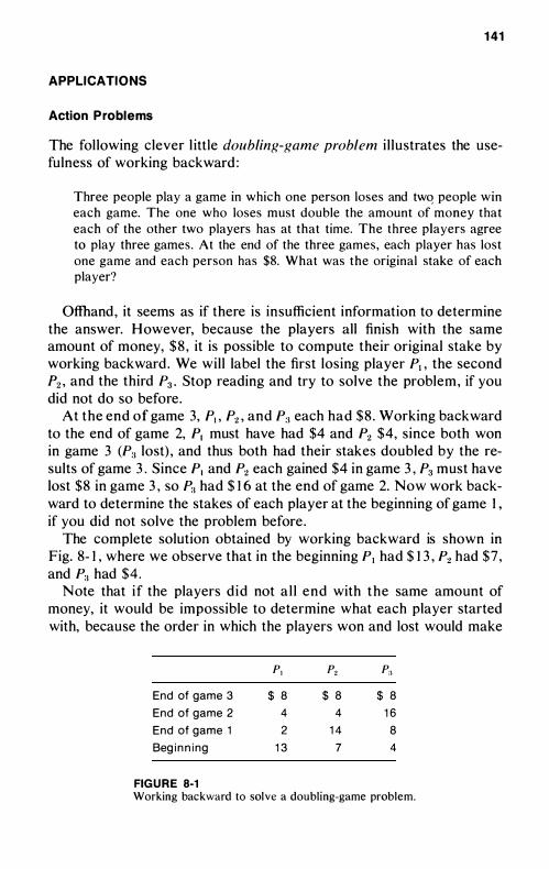
141

APPLICATIONS

Action Problems

The fol lowing clever l ittle doubling-game problem i l lustrates the use­fulness of working backward :

Three people play a game in which one person loses and twq people win each game. The one who loses must double the amount of money that each of the other two players has at that time. The three players agree to play three games . At the end of the three games, each player has lost one game and each person has $8. What was the original stake of each player?

Offhand, it seems as if there is insufficient information to determine the answer. However, because the players all finish with the same amount of money, $ 8 , it is possible to compute their original stake by working backward . We wil l label the first losing player PI , the second P2 , and the third P3 • Stop reading and try to solve the problem, if you did not do so before.

At the end of game 3, PI ' P2 , and p;! each had $8 . Working backward to the end of game 2, PI must have had $4 and P2 $4, since both won in game 3 (Pa lost) , and thus both had their stakes doubled by the re­suIts of game 3 . Since PI and P2 each gained $4 in game 3 , P3 must have lost $8 in game 3 , so Pa had $ 1 6 at the end of game 2. Now work back­ward to determine the stakes of each player at the beginning of game 1 , if you did not solve the problem before .

The complete solution obtained by working backward is shown in Fig. 8- 1 , where we observe that in the beginning PI had $ 1 3 , P2 had $7 , and Pa had $4 .

Note that i f the players d id not a l l end with the same amount of money, it would be impossible to determine what each player started with, because the order in which the players won and lost would make

PI P2 P"

End of game 3 $ 8 $ 8 $ 8

End of game 2 4 4 1 6

End of game 1 2 1 4 8

Beg i n n i ng 1 3 7 4

FIG U R E 8-1 Working backward to solve a doubling-game problem.

142 Chapter 8

a d ifference. However, in the present instance , the order in which the players won or lost games makes no difference to determining the initial stake of each player.

Also, if you had names for the players , you could not tell which player started with $ 1 3 , which with $7, and which with $4, unless you know the order in which they won. H ere I simply named the first losing player PI ' the second P2 , and the third Pa • This was completely ade­quate , since the stated goal did not require pairing stakes with named players.

This doubl ing-game problem is an extreme example of the useful­ness of working backward, since it is essential ly impossible to solve the problem, except by working backward . The reason is that there is a uniquely defined goal , but no given state is specified at al l . In fact, the problem is to derive a given state that, in conjunction with the op­erations, will produce the goal state . Although the operations are stated in a forward direction , they easily admit the definition of unique in­verse operations (in which two people have their stakes cut in half and the other person has his stake increased by the sum of the amounts the others were decreased) . Thus , it is clear we must use the method of working backward to solve thi s problem. Of course, it is equally correct to say that what we have done is to transform the operations into inverse operations and reverse the goal and the givens, taking the goal as the givens and attempting to derive the given state from the goal . Obviously, it makes l ittle difference which way we describe what was done in this problem, since what was done is precisely the same under either description .

Nim games are games in which each player takes away tokens sub­ject to a variety of restrictions and tries to be the last - or not the last - to take a token . N im games provide excellent examples of the usefulness of working backward to determine optimal strategy. One example is the following:

Fifteen pennies are placed on a table in front of two players. Each player is allowed to remove at least one penny but not more than five pennies at his tum. The p layers alternate turns , each removing from one to five pennies n number of turns, unti l one player takes the last penny on the table, and wins all 1 5 pennies . I s there a method of play that wi l l guarantee victory? I f so, what i s i t?

Stop reading and try to determine the optimal strategy by working backward .

If you conjecture yourself to be in the goal state , this state would

Working Backward 143

clearly consist of being the player whose turn it i s to move, and there being anywhere from one to five pennies on the table. I n this state, you could take all of the pennies left on the table and be the winner. Now, can you work backward from this set of possible goal states to conjecture a preceding state for the other player in which, no matter what that player does , you wil l be in one of these desirable goal states? Stop reading and try to solve the problem, i f you d id not before .

It i s c lear that if you confronted the opposing player with six pennies on the preceding turn , no matter how many pennies he or she took (from one to five, there would stil l be from one to five pennies on the table when it was your turn , giving you the victory. Thus , you should try to confront your opponent with six pennies after your move. But you cannot do this on your first move, so you must work backward again and ask what previous position you would have to put your opponent in so that, no matter what he did , you could have six pennies on the table after your move. Now stop reading and try to solve the rest of the problem, if you did not before .

Some thought reveals that i f you could confront the opposing player with 1 2 pennies after Y9ur preceding move, then no matter how many pennies he took (from 1 to 5), you would be able to take enough pennies to confront him with 6 pennies on the next turn. Thus , you want to confront your opponent with 1 2 pennies , and you can do that on your first move by removing 3 pennies from the board.

Note that in this nim problem, there was no uniquely defined goal state, since the goal is to take the last one, two, three , four, or five pen­nies on the table, and we cannot know which of these moves would con­stitute the goal in any nim game we might win. Of course, you could easily transform this into the unique goal of fac ing your opponent with a table having zero pennies on it on the other player's next move. Ob­viously, it makes no difference which way you look at this nim problem. The point is that working backward wil l frequently generate many possible preceding states , and this fact does not necessari ly invalidate the method of working backward . I n the present instance, working backward two steps yields a uniyue preceding number of pennies that you should confront your opponent with on the turn prior to your opponent 's last turn - namely, six pennies. Thus , considering only your own sequence of moves (rather than all the different moves that might be made by your opponent) , we see that the method of working backward in the present problem proceeds to get one preceding state from one succeeding state . Thus , working in the backward direction, the tree of possible states is continually being pinched back to a single state at every alternate move. The lesson in this problem is that you

1 44 Chapter 8

should not be too easily discouraged from working backward by a multiplic ity of preceding states , if this multiplicity is only a temporary phenomenon or a one-time sprouting of branches of the tree followed by no further increase. We cannot expect the method of working back­ward to always produce a single one-to-one chain of states back to the givens from the goal with no alternatives to investigate.

Working backward was preferable to working forward in the preced­ing problem because the number of d ifferent action sequences that had to be considered working backward was considerably smaller than the number that had to be considered working forward . You could, at every alternate move, determine a unique state in which you should be . This is the most general criterion for the appl icability of working backward , namely, that it produce a smaller space of alternative action sequences than would be produced by working forward . Sometimes working backward is preferable to working forward because it pro­duces a smaller set of action sequences to consider when combined with a hi l l-climbing approach . An example is provided by the fol lowing checker-rearrangement problem :

On an infinitely extended checkerboard , one is given three black checkers and two white checkers init ial ly placed in immediately adjacent squares on a single row, proceeding from left to right, as shown in Fig. 8-2 : black (B) , white ( W) , black , white, black . The problem is to transform this arrangement of alternating black and white checkers into an arrange­ment in which all three black checkers are on the left and both white checkers are on the right (BBB W W), with all checkers being in adjacent squares and in the same row (see Fig. 8-2). The al lowable operation is to move two adjacent checkers at a time, one of which must be a black checker and one a white checker. During a move, the two checkers being moved must remain together at all t imes, with no reversal of their left­to-right order. You are permitted to move a white-black or black-white pair of checkers to any adjacent pair of unoccupied squares along the same line. Note that there is no need to keep the checkers that are not being moved in immediately adjacent squares at any time. That i s , there may be unoccupied squares between checkers at various stages between the givens and the goal . Also note that the five checkers in the goal state need not occupy the same five squares on the checkerboard as they did in the given state . They may occupy any immediately adjacent five squares in the same row.

Stop reading and try to solve the problem by defining an evaluation function and then using the method of working backward in conjunc­tion with a h il l-cl imbing approach on this evaluation function .

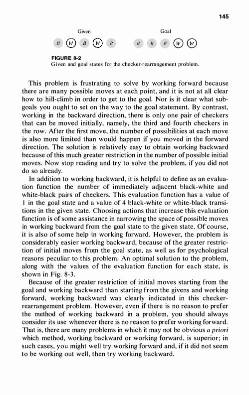
1 45

Given Goal

JJ IJ fl 0 0 FIG U R E 8-2 G iven and goal slates for the checker-rearrangement problem.

This problem is frustrating to solve by working forward because there are many possible moves at each point, and i t is not at all c lear how to h i ll-climb in order to get to the goal . Nor is it clear what sub­goals you ought to set on the way to the goal statement. By contrast, working in the backward direction, there is only one pair of checkers that can be moved initially, namely, the third and fourth checkers in the row. After the first move, the number of possibil ities at each move is also more limited than would happen if you moved in the forward direction. The solution is relatively easy to obtain working backward because of this much greater restriction in the number of possible initial moves . Now stop reading and try to solve the problem, if you d id not do so already.

In addition to working backward, it is helpfu l to define as an evalua­tion function the number of immediately adjacent black-white and white-black pairs of checkers. This evaluation function has a value of I in the goal state and a value of 4 black-white or white-black transi­tions in the given state . Choosing actions that increase this evaluation function is of some assistance in narrowing the space of possible moves in working backward from the goal state to the given state . Of course, i t i s also of some help in working forward. However, the problem is considerably easier working backward, because of the greater restric­tion of initial moves from the goal state , as wel l as for psychological reasons peculiar to this problem. An optimal solution to the problem, along with the values of the evaluation function for each state, is shown in Fig. 8-3 .

Because of the greater restriction of initial moves starting from the goal and working backward than starting from the givens and working forward , working backward was clearly indicated in this checker­rearrangement problem. However, even if there is no reason to prefer the method of working backward in a problem, you should always consider its use whenever there is no reason to prefer working forward. That is, there are many problems in which it may not be obvious a priori which method, working backward or working forward , is superior; in such cases , you might wel l try working forward and, if it did not seem to be working out well , then try working backward.

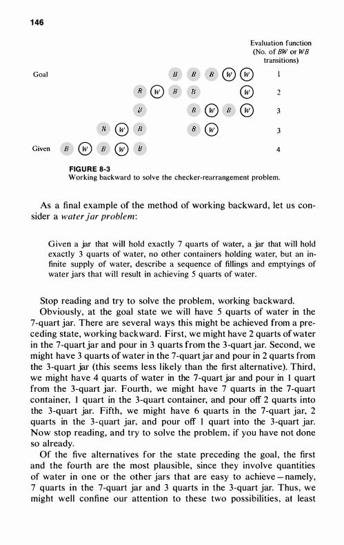
1 46

Goal B

/I e H

B

11 ® IJ

B B

f]

f] ® 11 ®

Evaluation function

(No. of BW or WB

transitions)

® ® ® 2

II ® 3

3

Given B e B ® }J 4

FIG U R E 8-3 Working backward to solve the checker-rearrangement problem.

As a final example of the method of working backward, let us con­sider a water jar problem :

Given a jar that will hold exactly 7 quarts of water, a jar that will hold exactly 3 quarts of water, no other containers holding water, but an in­finite supply of water, describe a sequence of fillings and emptyings of water jars that will result in achieving 5 quarts of water.

Stop reading and try to solve the problem, working backward. Obviously, at the goal state we wil l have 5 quarts of water in the

7-quart jar. There are several ways this might be achieved from a pre­ceding state, working backward . First, we might have 2 quarts of water in the 7 -quart jar and pour in 3 quarts from the 3 -quart jar. Second , we might have 3 quarts of water in the 7-quart jar and pour in 2 quarts from the 3 -quart jar (this seems less l ikely than the first alternative). Third , we might have 4 quarts of water in the 7 -quart jar and pour in I quart from the 3-quart jar. Fourth , we might have 7 quarts in the 7-quart container, ] quart in the 3 -quart container, and pour off 2 quarts into the 3 -quart jar. Fifth , we might have 6 quarts in the 7-quart jar, 2 quarts in the 3 -quart jar. and pour off I quart into the 3 -quart jar. Now stop reading, and try to solve the problem, if you have not done so already.

Of the five alternatives for the state preceding the goal , the first and the fourth are the most plausible, since they involve quantities of water in one or the other jars that are easy to achieve - namely, 7 quarts in the 7-quart jar and 3 quarts in the 3 -quart jar. Thus , we might well confine our attention to these two possibilities , at least

Working Backward 147

in itially. Now stop reading and try to solve the problem, if you have not done so already.

Although it is possible to achieve 2 quarts in a 7-quart jar as a sub­goal and fill up the 3 -quart jar as specified in the first alternative , the fourth alternative is actually optimal . Working backward from the fourth alternative (7 quarts in a 7-quart jar and I quart in the 3 -quart jar) , we set as the subgoal the achievement of 1 quart in either jar. It is probably not particularly usefu l to continue working backward any longer after having defined these five alternative preceding states . Rather, in attempting to achieve any one of these states , such as 7 quarts in the 7-quart jar and I quart in the 3 -quart jar, it is probably most useful to set th is as a subgoal and work forward from the given information in order to achieve it. In the present instance, it is quite easy to achieve the state of having 7 quarts in the 7-quart jar and 1 quart in the 3 -quart jar. To achieve I quart in the 3 -quart jar, fill the 7-quart jar, pour off 3 quarts two successive times to achieve 1 quart in the 7 -quart jar, then transfer this I quart to the 3 -quart jar. Now fil l up the 7-quart jar, and the subgoal is achieved. After thi s , of course , it is simple to pour off 2 quarts from the 7-quart jar into the 3 -quart jar, which already contains 1 quart. This leaves 5 quarts in the 7-quart jar, which is the goal .

This problem nicely i l lustrates how working backward can permit you to define a subgoal , which you can then achieve by working for­ward . This pattern is typical of working backward in both action prob­lems such as this one and the inference problems to be discussed next.

Inference Problems

As a simple example of the method of working backward in inference problems, consider the following proof problem:

If A > 0 and B > 0, then A 2 - AB + B2 > O. The theorem is actually true for a l l A and B, but it needless ly complicates the example of the method of working backward to consider the more general case. Thus , restrict the proof to the case where A > 0 and B > O.

Stop reading and try to solve the problem by working backward . To apply the method of working backward , we first state the conclu­

sion A2 - A B + B2 > O. A preceding statement that would imply that conclusion can be obtained by factoring the expression A 2 - A B + B2 into A (A - B) + B2 > O. If we could show this expression to be true,

148 Chapter 8

then it would imply the desired conclusion. Stop reading and try to solve the problem, if you d id not do so before .

By working backward we note that we cou ld derive the expression A (A - B ) + B2 > 0 from three previous expressions : first, A > 0, which i s given information ; second, B2 > 0 , which is true for all real numbers including B ; and , third , A - B > O. We cannot derive A - B > 0 from the given information, but we could just assume it as one case. Obviously, in some cases where both A > 0 and B > 0, A will be greater than B. So in the case where A > B, then A - B > 0, and the theorem is proved . Stop reading and try to solve the problem, if you did not before .

Now, work backward from the goal statement A 2 - A B + B2 > 0 to try to derive the goal expression in the case where B > A . I n this case, we factor the goal expression into A 2 + B ( B - A ) > 0, which will be true if, first, B > 0 (given information) ; second, A 2 > 0 (true for all real A ) ; and , third , B - A > O. Now, B - A > 0 fol lows from B > A . Thus , w e have established that the conclusion fol lows where A > B or B > A . I n addition, we have to show that the conclusion fol lows when A = B, but this matter i s trivial . This problem is so short and relatively trivial that many people may not notice how much they are working backward in solving it . H owever, a careful examination re­veals that the critical insights come from focusing on the goal statement and noticing what it can be factored into.

Frequently we use the method of working backward for only a few steps in order to derive some more congenial formulation of the state­ment to be proved, then we proceed to work in a forward direction in try ing to derive this more congenial formulation. Working backward may simply result in the substitution of a single subgoal (directly re­lated to the goal) for the original goal , or it may result in the substitu­tion of two or more subgoals in place of the original goal .

An extremely simple proof of the Pythagorean Theorem can be obtained by initially working backward from the algebraic goal state­ment to obtain a single, more geometric sub goal .

As you may remember, the Pythagorean Theorem states that, for any right triangle, c2 = {/2 + b2, where c is the length of the hypotenuse. Prove th is theorem, where the givens are , first, the axioms of Eucl idean geom­etry ; second, the definition of the area of a rectangular figure ( length times width) ; and , third , the assumption that the areas of nonoverlapping figures are additive.

Stop reading and try to prove the theorem by working backward to obtain a single subgoal .

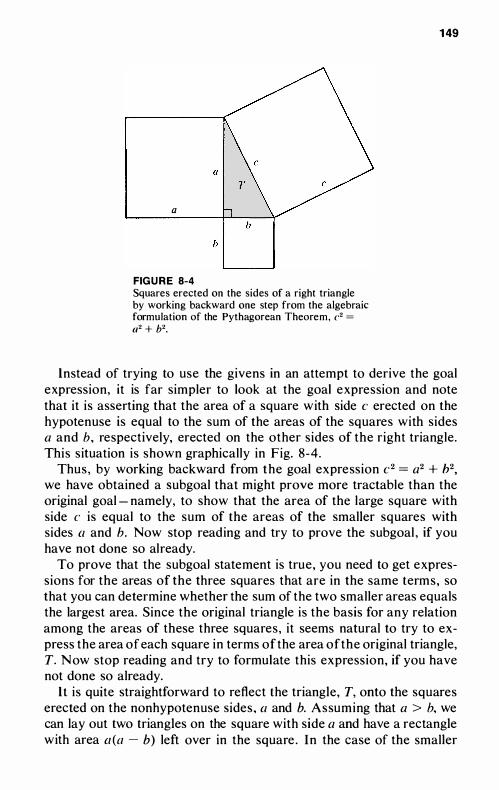
a

FIG U R E 8-4 Squares erected on the sides of a right triangle by working backward one step from the algebraic. formulation of the Pythagorean Theorem, c2 =

a2 + b2•

1 49

Instead of trying to use the givens in an attempt to derive the goal expression, it is far simpler to look at the goal expression and note that it is asserting that the area of a square with side c erected on the hypotenuse is equal to the sum of the areas of the squares with sides a and b, respectively, erected on the other sides of the right triangle. This situation is shown graphically in Fig. 8-4 .

Thus , by working backward from the goal expression c2 = a2 + b2, we have obtained a subgoal that might prove more tractable than the original goal - namely, to show that the area of the large square with side c is equal to the sum of the areas of the smaller squares with sides {/ and h. Now stop reading and try to prove the subgoal , if you have not done so already.

To prove that the subgoal statement is true, you need to get expres­sions for the areas of the three squares that are in the same terms, so that you can determine whether the sum of the two smaller areas equals the largest area. Since the original triangle is the basis for any relation among the areas of these three squares , it seems natural to try to ex­press the area of each square in terms of the area of the original triangle, T. Now stop reading and try to formulate this expression, if you have not done so already.

It is quite straightforward to reflect the triangle, T, onto the squares erected on the nonhypotenuse sides , (/ and b. Assuming that a > b, we can lay out two triangles on the square with side a and have a rectangle with area lI (a - b) left over in the square . In the case of the smaller

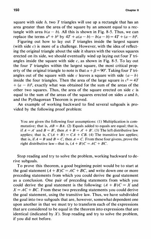
150 Chapter 8

square with side b, two T triangles wi l l u se up a rectangle that has an area greater than the area of the square by an amount equal to a rec­tangle with area b (a - b). All this is shown in Fig. 8-5 . Thus , we can replace the terms a2 + b2 by 4T + a (a - b) - b(a - b) = 4T + (a - b)2.

Figuring out how to lay out T triangles inside the largest square (with side c) is more of a challenge . However, with the idea of reflect­ing the original triangle about the side it shares with the various squares erected on its side, we should eventual ly wind up laying out four T tri­angles inside the square with side c, as shown in Fig. 8-5 . To lay out the four T triangles within the largest square , the most critical prop­erty of the original triangle to note is that ex + f3 = 90°. Taking four T tri­angles out of the square with side c leaves a square with side ( a - b ) inside the four triangles. Then the area of the large square i s c2 = 4 T + (a - b)2, exactly what was obtained for the sum of the areas of the other two squares . Thus, the area of the square erected on side c is equal to the sum of the areas of the squares erected on sides a and b, and the Pythagorean Theorem is proved .

An example of working backward to find several subgoals is pro­vided by the fol lowing proof problem:

You are given the following four assumptions : ( I ) Mult ipl ication is com­mutative ; that is, A B = BA . (2) Equals added to equals are equal ; that i s , if A = A ' and B = B' , then A + B = A' + B' . (3 ) The left distributive law applie s ; that is, C (A + B ) = CA + CB. (4) The transitive law applies ; that i s , if A = B and B = C, then A = C. From these four givens, prove the right distributive law - that is, (A + B ) C = A C + Be.

Stop reading and try to solve the problem, working backward to de­rive subgoals .

To prove this theorem, a good beginning point would be to start at the goal statement (A + B ) C =A C + BC, and write down one or more preceding statements from which you could derive the goal statement as a conclusion. One pair of preceding statements from which you could derive the goal statement is the following: (A + B ) C = X and X = A C + BC. From these two preceding statements you could derive the goal statement, using the transitive law. Thus, we have subdivided the goal into two subgoals that are , however, somewhat dependent one upon another in that we must try to transform each of the expressions that are considered to be equal in the theorem into expressions that are identical (indicated by X) . Stop reading and try to solve the problem, if you did not before.

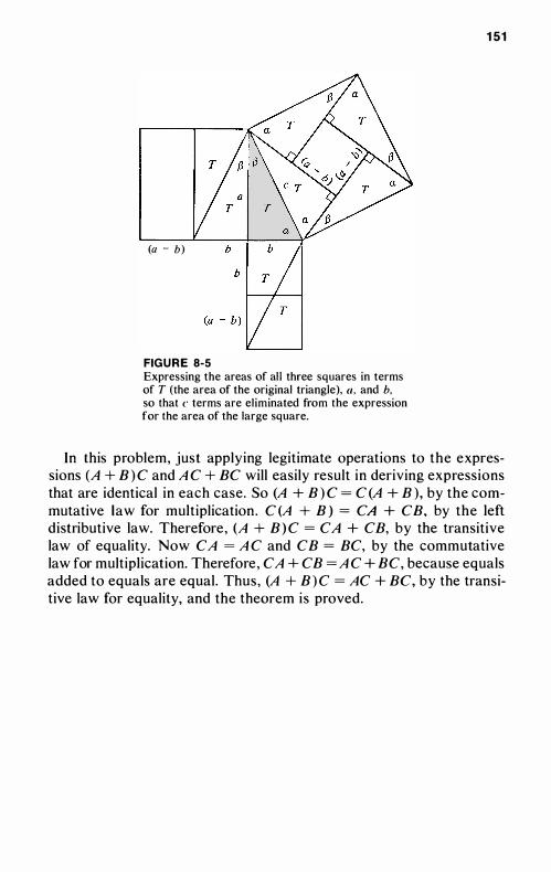
(a - b)

FIG U R E 8-5 Expressing the areas of al l three squares in terms of T (the area of the original triangle). c/ . and b. so that c terms are el iminated from the expression for the area of the large square.

151

In this problem, just applying legitimate operations to the expres­sions (A + B ) C and A C + BC will easily result in deriving expressions that are identical in each case. So (A + B ) C = C (A + B ), by the com­mutative law for multiplication . C (A + B ) = CA + CB, by the left distributive law. Therefore , (A + B ) C = CA + CB, by the transitive law of equality. Now CA = A C and CB = BC, by the commutative law for multiplication. Therefore , CA + C B = A C + BC, because equals added to equals are equal. Thus , (A + B ) C = AC + BC, by the transi­tive law for equality, and the theorem is proved.

9

Relations Between Problems

When mankind has a satisfactory theory of problems, it wil l be pos­sible to state many deep and detailed relations between d ifferent types of problems. But even without such a theory, we can stil l state certain basic types of relations between d ifferent problems.

In particular, five fundamental types of relations can obtain between two problems, a and b: First, problem a is unrelated to problem b (problem a and problem b have no common elements). Second , prob­lem a is equivalent to problem b (a and b have the same problem ele­ments, a and b are completely analogous , a and b are isomorphic). Third , problem a i s similar to problem b (problems a and b have some common e lements, problems a and b are partially analogous). Fourth , problem a is a special case of problem b (problem a is included in problem b) . Fifth , problem a is a generalization of problem b (problem b is included in problem a ) . When problems a and b are similar, they may be of approximately equivalent difficulty, b may be simpler than a, or b may be more complex than a .

EQUIVALENT PROBLE MS

In determining whether any of these five relations holds between two problems, it is important to note that the critical problem elements

Relations Between Problem s 1 53

concern the types of operations and the relations that can obtain be­tween different expressions or things, not the specific expressions or things themselves. For example, in the checker-rearrangement prob­lem described in Chapter 8, it would make no difference in the e lements of that problem, from a problem-solving viewpoint, if the black checkers were changed to quarters and the white checkers were changed to pennies, provided that all the same restrictions and opera­tions stil l applied. Alternatively, we could replace the black checkers by red poker chips and the white checkers by blue poker chips, and , i f everything else remained the same, the problem would be equivalent to the original problem. Similarly, in the nim problem of Chapter 8 , i n which from one to five pennies were removed by a player o n each turn, the pennies could be replaced by any token such as marbles, poker chips, buttons , or stones . In the Tower of Hanoi problem in Chapter 6, the disks of decreasing s ize could be replaced by any set of tokens having a simple order relation among them.

Problems that differ only with respect to the names attached to different elements of the problem, but all of whose relations and opera­tions are identical, are considered equivalent, meaning they are completely analogous or isomorphic. Recognizing that two problems are equivalent may sometimes involve realizing that many of the im­plied properties indicated by the d ifferent names attached to corre­sponding elements in the two problems are completely irrelevant to the solution of the problem. However, it is usually relatively trivial to recognize such irrelevancies of the differing properties of corre­sponding elements, and consequently the recognition of equivalent problems is frequently trivial .

SIMILAR PROBLEMS

Two problems can be extremely similar and yet not be equivalent in every respect. For example, in the Tower of Hanoi problem, you may start with 5, 6, 7, or 1 0 disks on a single spike ; the number of disks you begin with is in no way critical to the method of solving the prob­lem as outlined in Chapter 6 . You can , in fact, state a solution to the general Tower of Hanoi problem in which n disks must be transferred from one spike to another. Thus, any particular Tower of H anoi prob­lem (a problem involving the transfer of some particular number of disks from one spike to another) is a special case of the general Tower of Hanoi problem. Any two special cases of the general Tower of Hanoi problem are simi lar problems, though I would hesitate to call them equivalent problems.

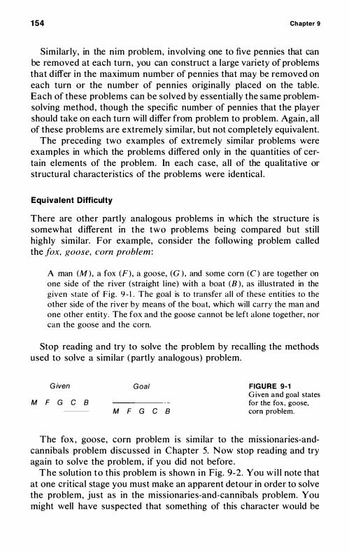
154 Chapter 9

Similarly, in the nim problem, involving one to five pennies that can be removed at each turn, you can construct a large variety of problems that d iffer in the maximum number of pennies that may be removed on each turn or the number of pennies originally placed on the table. Each of these problems can be solved by essential ly the same problem­solving method, though the specific number of pennies that the player should take on each turn will differ from problem to problem. Again , all of these problems are extremely similar, but not completely equivalent.

The preceding two examples of extremely similar problems were examples in which the problems d iffered only in the quantities of cer­tain elements of the problem. In each case, all of the qualitative or structural characteristics of the problems were identical .

Equ ivalent Difficulty

There are other partly analogous problems in which the structure is somewhat d ifferent in the two problems being compared but still highly similar. For example, consider the following problem called the fox, goose, corn problem :

A man (M ) , a fox (F) , a goose, (G ) , and some corn (C ) are together on one side of the river (straight l ine) with a boat (8 ) , as i l lustrated in the given state of Fig . 9 - \ . The goal is to transfer a l l of these entit ies to the other side of the river by means of the boat, which will carry the man and one other ent i ty . The fox and the goose cannot be left alone together, nor can the goose and the corn.

Stop reading and try to solve the problem by recalling the methods used to solve a similar (partly analogous) problem.

G iven G oal

M F G C B M F G C B

FIG U R E 9-1 G iven and goal states for the fox , goose, corn problem.

The fox , goose, corn problem is similar to the missionaries-and­cannibals problem discussed in Chapter 5. Now stop reading and try again to solve the problem, if you did not before .

The solution to this problem is shown in Fig. 9-2 . You wi l l note that at one critical stage you must make an apparent detour in order to solve the problem, just as in the missionaries-and-cannibals problem. You might well have suspected that something of this character would be

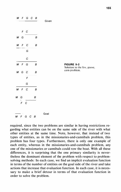
155

M F G C B G iven

F C

M G B

M F C B

G

C

M F G B FIG U R E 9 - 2 Sol ut ion to the fox , goose ,

M G C B corn p roblem.

F

G

M F C B

M G B

F C

Goal M F G C B

required , since the two problems are similar in having restrictions re­garding what entities can be on the same side of the river with what other entities at the same time. Note, however, that instead of two types of entities , as in the missionaries-and-cannibals problem, this problem has four types . Furthermore , there is only one example of each entity, whereas in the missionaries-and-cannibals problem, any one of the missionaries or cannibals could row the boat. With all these differences, it is surprising that the one primary similarity is never­theless the dominant element of the problem with respect to problem­solving methods : In each case, we find an implicit evaluation function in terms of the number of entities on the goal side of the river and take actions that increase that evaluation function. In each case , it is neces­sary to make a brief detour in terms of that evaluation function in order to solve the problem.

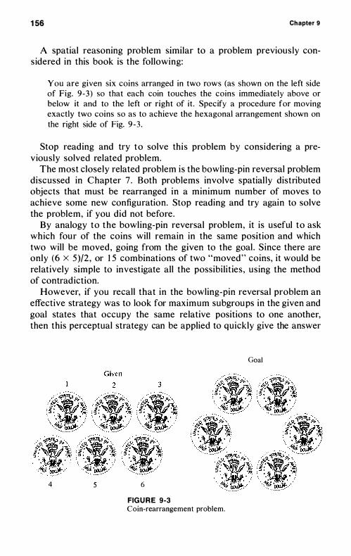
1 56 Chapter 9

A spatial reasoning problem similar to a problem previous ly con­sidered in this book is the following:

You are given six coins arranged in two rows (as shown on the left side of Fig. 9-3) so that each coin touches the coins immediately above or below it and to the left or right of it . Specify a procedure for moving exactly two coins so as to achieve the hexagonal arrangement shown on the right side of Fig. 9 -3 .

Stop reading and try to solve this problem by considering a pre­viously solved related problem.

The most closely related problem is the bowling-pin reversal problem discussed in Chapter 7 . Both problems involve spatial ly distributed objects that must be rearranged in a minimum number of moves to achieve some new configuration. Stop reading and try again to solve the problem, if you did not before .

By analogy to the bowling-pin reversal problem, it is useful to ask which four of the coins will remain in the same position and which two will be moved, going from the given to the goal . Since there are only (6 X 5)/2 , or 1 5 combinations of two "moved" coins, it would be relatively simple to investigate all the possibilities , using the method of contradiction.

However, if you recall that in the bowling-pin reversal problem an effective strategy was to look for maximum subgroups in the given and goal states that occupy the same relative positions to one another, then this perceptual strategy can be applied to quickly give the answer

4 5 6

FIG U R E 9-3 Coin-rearrangement problem.

Goal

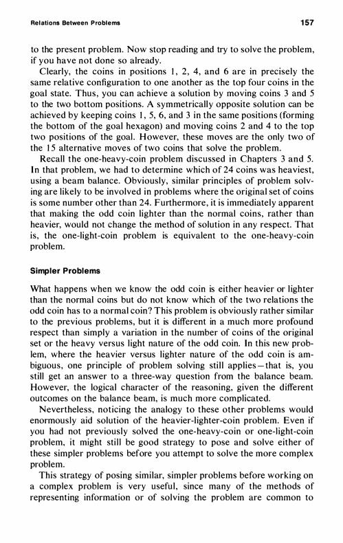
Relations Between Problems 157

to the present problem. Now stop reading and try to solve the problem, if you have not done so already.

Clearly, the coins in positions 1 , 2 , 4, and 6 are in precisely the same relative configuration to one another as the top four coins in the goal state. Thus , you can achieve a solution by moving coins 3 and 5 to the two bottom positions. A symmetrically opposite solution can be achieved by keeping coins 1 , 5, 6, and 3 in the same positions (forming the bottom of the goal hexagon) and moving coins 2 and 4 to the top two positions of the goal . H owever, these moves are the only two of the 1 5 alternative moves of two coins that solve the problem.

Recall the one-heavy-coin problem discussed in Chapters 3 and 5. In that problem, we had to determine which of 24 coins was heaviest, using a beam balance. Obviously, similar principles of problem solv­ing are likely to be involved in problems where the original set of coins is some number other than 24. Furthermore , it is immediately apparent that making the odd coin lighter than the normal coins , rather than heavier, would not change the method of solution in any respect. That is , the one-light-coin problem is equivalent to the one-heavy-coin problem.

Simpler Problems

What happens when we know the odd coin is either heavier or l ighter than the normal coins but do not know which of the two relations the odd coin has to a normal coin? This problem is obviously rather similar to the previous problems, but it is d ifferent in a much more profound respect than simply a variation in the number of coins of the original set or the heavy versus l ight nature of the odd coin. In this new prob­lem, where the heavier versus l ighter nature of the odd coin is am­biguous , one principle of problem solving sti l l applies - that is, you still get an answer to a three-way question from the balance beam. However, the logical character of the reasoning, given the d ifferent outcomes on the balance beam, is much more complicated.

Nevertheless , noticing the analogy to these other problems would enormously aid solution of the heavier-l ighter-coin problem. Even if you had not previously solved the one-heavy-coin or one-l ight-coin problem, it might sti l l be good strategy to pose and solve either of these simpler problems before you attempt to solve the more complex problem.

This strategy of posing simi lar, simpler problems before working on a complex problem is very usefu l , since many of the methods of representing information or of solving the problem are common to

1 58 Chapter 9

both . To be sure, the complex problem will invariably have some additional complications. However, if when solving the simpler prob­lem you d iscovered some of the methods for solving the complex problem, it will be easier to discover the remaining methods of solv­ing the more complex problem than if you had to solve the complex problem as a whole.

Along the same lines, when you original ly confronted the one-heavy­coin problem with a set of 24 coins, you might have tried solving a simpler problem, with the odd coin embedded in a set of only three or four coins. With a set of three coins, you have the best opportunity to real ize that the balance beam can provide a three-way partitioning of the set of alternatives .

Often , as in the heavy-coin problems, you judge the simplicity of the problem by the number of d ifferent elements or complications in it. In the one-heavy-coin problems, which differ only in the total size of the original set of coins , the complication of the problem seems to be variable in a simple way, namely, the change in the number of coins in the total set.

H owever, we have also noted that a problem in which the odd coin might be either heavier or l ighter was a substantial l y more complicated problem than the problem in which it was known definitely which weight relation the odd coin had to a normal coin. Simplicity in a prob­lem is by no means a simple quantitative concept.

Another problem similar to the one-heavy-coin problem, but simpler to solve because it has one less restriction, is the problem of three-way­question information theory. The problem is to determine which element is the unique element, in a set of n possible elements, by successively partitioning the set into three subsets , then ask which of the three subsets contains the unique element.

In ordinary (two-way-question) information theory, the optimal strategy is to divide the total set into two equal or nearly equal parts and to continue dividing the remaining set into two equal parts until the unique element i s determined . Interestingly, in three-way-question information theory, the optimal strategy is not always to divide into three equal (or nearly equal) parts , though this is not a bad strategy. If the objective is to minimize the expected number of questions to be asked in order to determine the unique element, then other kinds of partitions besides the equal partition are optimal for some set sizes. For example, if there are six elements in the original total set, the opti­mal strategy with three-way-question information theory is not to divide into 2, 2, and 2 on the first partition. Instead , the optimal strategy is to divide into 3 , 2, and 1 , because one-sixth of the time this will

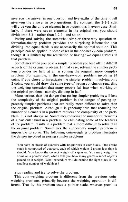
Relations Between Problems 1 59

give you the answer in one question and five-sixths of the time it wil l give you the answer in two questions. By contrast, the 2-2-2 spl it will give you the unique element in two questions in every case . Simi­larly, if there were seven elements in the original set , you should divide into 3-3- 1 rather than 3-2-2 - and so on.

Posing and solving the somewhat simpler three-way question in­formation-theory problem provides the surprising information that dividing into equal thirds is not necessari ly the optimal solution. This principle can be applied in some cases in the one-heavy-coin problem, though it is limited by the restriction of having two equal subsets in that problem.

Sometimes when you pose a simpler problem you lose all the difficult aspects of the original problem. In that case, solving the simpler prob­lem provides no help at all in solving the original , more complex problem. For example, in the one-heavy-coin problem involving 24 coins, if you chose to investigate the simpler problem involving only 2 coins, you would draw the same type of wrong conclusion regarding the weighing operation that many people fall into when working on the original problem - namely, dividing in half.

More serious than the danger that posing simpler problems wil l lose the complexity of the original problem is the danger of posing ap­parently simpler problems that are really more difficult to solve than the original problem. Although it is general ly true that reducing the number of elements in a problem reduces the complexity of the prob­blem, it is not always so. Sometimes reducing the number of elements of a particular kind in a problem, or el iminating some of the features of the problem, results in a problem that is more difficult to solve than the original problem. Sometimes the supposedly simpler problem is impossible to solve. The following coin-weighing problem i l lu strates the danger involved in posing simpler problems :

You have 10 stacks of quarters with 10 quarters in each stack. One entire stack is composed of quarters, each of which weighs 2 grams less than i t should. You know the correct weight of a quarter. You may weigh the coins on a pointer scale , which tel ls you how many grams a set of objects placed on it weighs. What procedure wi l l determine the l ight stack in the smallest number of weighings?

Stop reading and try to solve the problem. This coin-weighing problem is different from the previous coin­

weighing problems, primari ly because the weighing operation is dif­ferent. That is , this problem uses a pointer scale, whereas previous

160 Chapter 9

problems used a beam balance . A weighing operation using a beam balance provides an answer to a three-way question , but a single weighing on a pointer scale provides an enormously greater amount of information ( l imited only by the accuracy of the pointer scale) . Because of the great difference in the amount of information provided by the pointer versus beam-balance weighings, there is virtual ly no similarity between the solutions to these two types of coin-weighing problems. Thus , these two types of coin-weighing problems are not real ly related at al l , in the problem-solving sense. The presence or absence of concrete similarities , such as two problems being both concerned with coins and weighing operations, is less important than more abstract similarities concerned with the relationships among givens or between givens and operations. If you were misled into trying to apply similar methods to those used in solving the previous coin-weighing problems, stop reading and try again to solve this problem.

Another approach that fai l s is to try to simplify the problem by re­ducing the number of coins in each stack to one coin and simply deter­mining which of the 1 0 remaining coins is l ight. This actually makes the number of weighings vastly greater than in the original problem, where one had 1 0 stacks of 10 coins each. What other way is there to simplify the problem? Stop reading and try again to solve the problem, if you did not before.

The other obvious way to simplify the problem is to reduce the num­ber of stacks . Solving a problem with a reduced number of stacks could faci l itate solution of the problem. Now stop reading and try to solve the problem, using this method of simpl ification , if you did not solve it before .

The simplest problem that can be posed , reducing the number of stacks , is to decide which of two stacks is l ight. Evidently, this could be done in one weighing by weighing a single coin from one of the two stacks and determining that it is either the correct weight for a quarter or 2 grams less than the correct weight. Of itself, this solution to the two-stack problem does not indicate how you should solve the 1 0-stack problem. However, it does provide you with a basic familiarity re­garding the nature of the information provided by the pointer scale. You should then try to solve a three-stack problem. Now stop reading and try to solve the three-stack problem in a way that will allow gen­eralization to a 1 0-stack problem, if you have not solved the problem so far.

The three-stack problem can be solved in a single weighing, as can the 1 0-stack problem. However, an insight is required to accomplish this . I know of no general problem-solving method that would auto-

Relations Between Problems 161

matically provide you with the critical insight. Attempting to solve the simpler three-stack problem makes it more l ikely that you would achieve that insight, but it does not guarantee it . If you have not yet solved the problem, stop reading and try to determine what combina­tion of coins from the different stacks would allow you to determine which of the three stacks was the l ight stack in a single weighing. Once the three-stack problem is solved , the same procedure wil l im­mediately generalize to the 1 0-stack problem.

The three-stack problem can be solved in a single weighing only by including some number of coins from each stack and using the amount of underweight as measured by the pointer scale to determine which of the stacks is l ight. To make use of the information concerning the number of grams by which the weighing is underweight (from what it would be if the coins were all true quarters) , we clearly need to have some way of associating the amount of underweight with each of the three stacks. This type of reasoning is an i l lustration of drawing in­ferences from the goal (determining the l ight stack in a single weigh­ing) . Again stop reading and try to solve the problem, if you have not done so already.

The procedure required to associate each stack with an amount of underweight is to take one coin from the first stack, two from the second stack, and three from the third . If the pointer scale reads 2 grams underweight, you know that the first stack is l ight. If it reads 4 grams underweight, the second stack is light. If it reads 6 grams un­derweight, the th ird stack is light. Generalize the solution to the 1 0-stack problem, if you have not done so already.

The original 1 0-stack problem is solved in a single weighing as fol­lows : You take one coin from stack 1 , two coins from stack 2 , three coins from stack 3 , and so on, up to 1 0 coins from stack 1 0 . Now weigh this entire set of coins and determine by how many grams it is underweight. The number of grams of underweight d ivided by 2 is the number of the stack that is l ight. Thus , the solution can be achieved with only a single weighing, when you have a sufficiently large number of coins available in each stack . Reducing the number of coins in each stack does not simpl ify the problem; indeed , it makes the problem much more difficult, to the point of completely preventing you from seeing the elegant solution to the original problem. When you reduce the number of stacks rather than the number of coins in each stack, you obtain problems that are in some sense simpler, though , of course , you cannot reduce the number of weighings below 1 .

Reducing the number of elements i n a problem i s not the only way to make it simpler. Another way is to change the problem so as to allow you to use an already proved theorem in the solution. That is, you

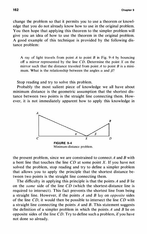
162 Chapter 9

change the problem so that it permits you to use a theorem or knowl­edge that you do not already know how to use in the original problem. You then hope that applying this theorem to the simpler problem will give you an idea of how to use the theorem in the original problem. A good example of this technique is provided by the fol lowing dis­tance problem :

A ray of l ight travels from point A to point B in Fig. 9 -4 by bouncing off a mirror represented by the line CD. Determine the point X on the mirror such that the distance traveled from point A to point B i s a mini­mum. What is the relationship between the angles a and f3?

Stop reading and try to solve this problem. Probably the most salient piece of knowledge we all have about

minimum distance is the geometric assumption that the shortest dis­tance between two points is the straight l ine connecting them. How­ever, it is not immediately apparent how to apply this knowledge in

c x FIG U R E 9-4 M inimum-di stance problem.

D

the present problem, since we are constrained to connect A and B with a bent line that touches the line CD at some point X. If you have not solved the problem, stop reading and try to define a simpler problem that allows you to apply the principle that the shortest distance be­tween two points is the straight l ine connecting them.

The difficulty in applying this principle is that the points A and B lie on the same side of the l ine CD (which the shortest-distance l ine is required to intersect ) . This fact prevents the shortest l ine from being a straight l ine . However, if the points A and B lay on opposite sides of the line CD, it would then be possible to intersect the line CD with a straight l ine connecting the points A and B. This statement suggests the definition of a simpler problem in which the points A and B lie on opposite sides of the l ine CD. Try to define such a problem, if you have not done so already.

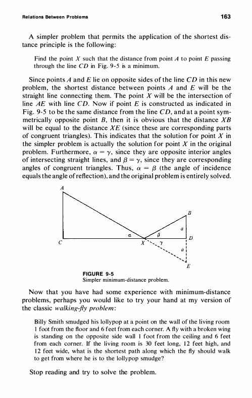
Relations Between Problems 1 63

A simpler problem that permits the application of the shortest dis­tance principle is the fol lowing :

Find the point X such that the d istance from point A t o point E pass ing through the line CD in Fig. 9 -5 is a minimum.

Since points A and E l ie on opposite sides of the l ine CD in this new problem, the shortest distance between points A and E will be the straight line connecting them. The point X will be the intersection of l ine AE with line CD. N ow if point E i s constructed as indicated in Fig . 9-5 to be the same d istance from the l ine CD, and at a point sym­metrically opposite point B, then it i s obvious that the d istance X B wil l be equal to the d istance XE (since these are corresponding parts of congruent triangles) . This ind icates that the solution for point X in the simpler problem is actual ly the solution for point X in the original problem. Furthermore , ex = y, since they are opposite interior angles of intersecting straight l ines, and f3 = y, since they are corresponding angles of congruent triangles . Thus , ex = f3 (the angle of incidence equals the angle of reflection) , and the original problem is entire ly solved.

A

a �--------------�--���------�, D

C X � � _ 'Y I

FIG U R E 9-5

... .... ... .... I ... .... a I � � � � : � �

E

Simpler minimum-distance problem.

Now that you have had some experience with minimum-distance problems, perhaps you would like to try your hand at my version of the classic walking-fly problem :

Bi l ly Smith smudged h i s lol lypop at a point on the wall of the living room I foot from the floor and 6 feet from each corner. A fly with a broken wing is standing on the opposite side wall I foot from the cei l ing and 6 feet from each corner. If the l iv ing room is 30 feet long, 1 2 feet high , and 1 2 feet wide, what is the shortest path along which the fly should walk to get from where he i s to the lollypop smudge?

Stop reading and try to solve the problem.

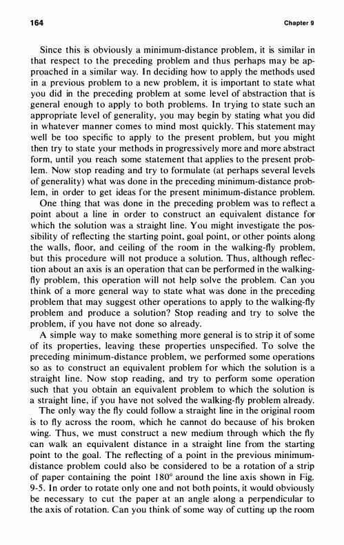
1 64 Chapter 9

Since this is obviously a minimum-distance problem, it is simi lar in that respect to the preceding problem and thus perhaps may be ap­proached in a similar way. I n deciding how to apply the methods used in a previous problem to a new problem, it is important to state what you did in the preceding problem at some level of abstraction that is general enough to apply to both problems. I n trying to state such an appropriate level of general ity, you may begin by stating what you did in whatever manner comes to mind most quickly. This statement may well be too specific to apply to the present problem, but you might then try to state your methods in progressively more and more abstract form, until you reach some statement that applies to the present prob­lem. Now stop reading and try to formulate (at perhaps several levels of general ity) what was done in the preceding minimum-di stance prob­lem, in order to get ideas for the present minimum-distance problem.

One thing that was done in the preceding problem was to reflect a point about a l ine in order to construct an equivalent di stance for which the solution was a straight l ine. You might investigate the pos­sibil ity of reflecting the starting point, goal point, or other points along the wall s , floor, and ceil ing of the room in the walking-fly problem, but this procedure wil l not produce a solution. Thus , although reflec­tion about an axis is an operation that can be performed in the walking­fly problem, this operation wil l not help solve the problem. Can you think of a more general way to state what was done in the preceding problem that may suggest other operations to apply to the walking-fly problem and produce a solution? Stop reading and try to solve the problem, if you have not done so already.

A simple way to make something more general is to strip it of some of its properties , leaving these properties unspecified . To solve the preceding minimum-distance problem, we performed some operations so as to construct an equivalent problem for which the solution is a straight l ine . Now stop reading, and try to perform some operation such that you obtain an equivalent problem to which the solution is a straight l ine, if you have not solved the walking-fly problem already.

The only way the fly could follow a straight line in the original room is to fly across the room, which he cannot do because of h is broken wing. Thus , we must construct a new medium through which the fly can walk an equivalent d istance in a straight l ine from the starting point to the goal . The reflecting of a point in the previous minimum­distance problem could also be considered to be a rotation of a strip of paper containing the point 1 800 around the l ine ax is shown in Fig. 9-5 . I n order to rotate only one and not both points, it would obviously be necessary to cut the paper at an angle along a perpendicular to the axis of rotation. Can you think of some way of cutting up the room

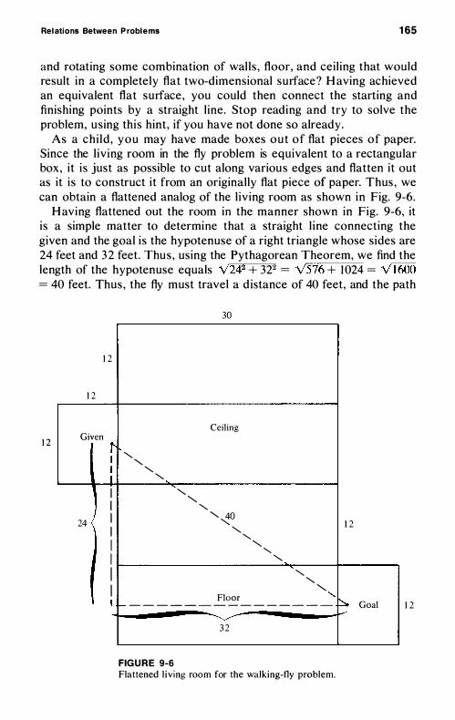
Relations Between Problems 165

and rotating some combination of wal ls , floor, and cei l ing that would result in a completely flat two-dimensional surface? H aving achieved an equivalent flat surface , you could then connect the starting and finishing points by a straight l ine. Stop reading and try to solve the problem, using this hint, if you have not done so already .

As a ch i ld , you may have made boxes out of flat pieces of paper. Since the l iv ing room in the fly problem is equivalent to a rectangular box , it i s just as possible to cut along various edges and flatten it out as it i s to construct it from an originally flat piece of paper. Thus , we can obtain a flattened analog of the l iv ing room as shown in Fig. 9-6.

H aving flattened out the room in the manner shown in Fig. 9-6, it is a simple matter to determine that a straight l ine connecting the given and the goal i s the hypotenuse of a right triangle whose sides are 24 feet and 3 2 feet. Thus , using the Pythagorean Theorem, we find the length of the hypotenuse equals v'242 + 322 = v'576 + 1 024 = v'1600 = 40 feet. Thus , the fly must travel a d istance of 40 feet, and the path

30

1 2

12

Ceiling

12 Given

i "'- "'-: "'- "'-I "'-I "'- "'-I "'- 40 24 " 1 2 I "'- " I "'- " I "'-I "'- "'-I "'-

Floor " I � _ _ _ _ _ - - - - - - - - - - f:- Goal 1 2

3 2

FIG U R E 9-6

Flattened l i v i ng room for the walking-fly problem.

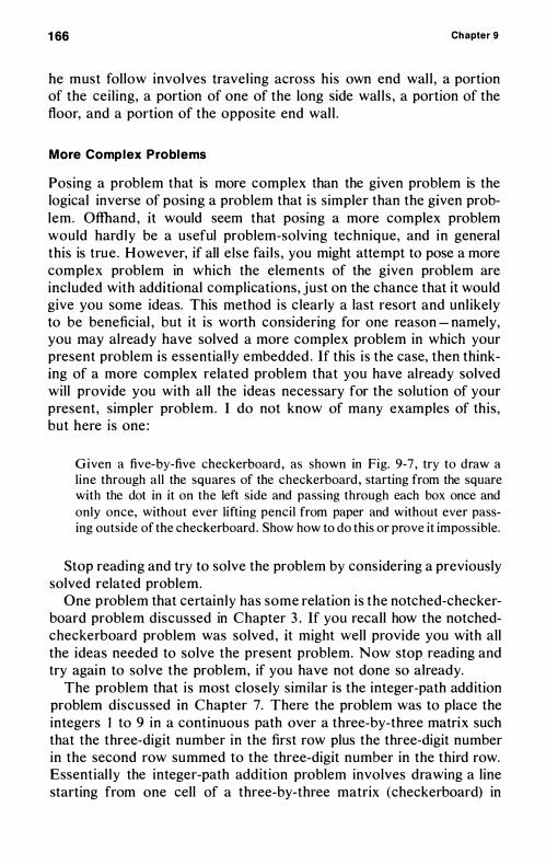
1 66 Chapter 9

he must follow involves travel ing across his own end wal l , a portion of the ceil ing, a portion of one of the long side wal ls , a portion of the floor, and a portion of the opposite end wal l .

More Complex Problems

Posing a problem that is more complex than the given problem is the logical inverse of posing a problem that is simpler than the given prob­lem. Offhand , it would seem that posing a more complex problem would hardly be a useful problem-solving technique, and in general this is true . However, if all else fai ls , you might attempt to pose a more complex problem in which the elements of the given problem are included with additional complications, just on the chance that it would give you some ideas. This method is c learly a last resort and unl ikely to be beneficial , but it is worth considering for one reason - namely, you may already have solved a more complex problem in which your present problem is essentially embedded . If this is the case, then think­ing of a more complex related problem that you have already solved will provide you with all the ideas necessary for the solution of your present, simpler problem. I do not know of many examples of this , but here is one :

Given a five-by-five checkerboard , as shown in Fig. 9-7 , try to draw a l ine through al l the squares of the checkerboard , starting from the square with the dot in it on the left side and passing through each box once and only once, without ever lifting pencil from paper and without ever pass­ing outside of the checkerboard . Show how to do this or prove it impossible.

Stop reading and try to solve the problem by considering a previously solved related problem.

One problem that certainly has some relation is the notched-checker­board problem discussed in Chapter 3 . If you recall how the notched­checkerboard problem was solved , it might well provide you with all the ideas needed to solve the present problem. Now stop reading and try again to solve the problem, if you have not done so already.

The problem that is most closely similar is the integer-path addition problem discussed in Chapter 7. There the problem was to place the integers 1 to 9 in a continuous path over a three-by-three matrix such that the three-digit number in the first row plus the three-digit number in the second row summed to the three-digit number in the third row. Essential ly the integer-path addition problem involves drawing a line starting from one cell of a three-by-three matrix (checkerboard) in

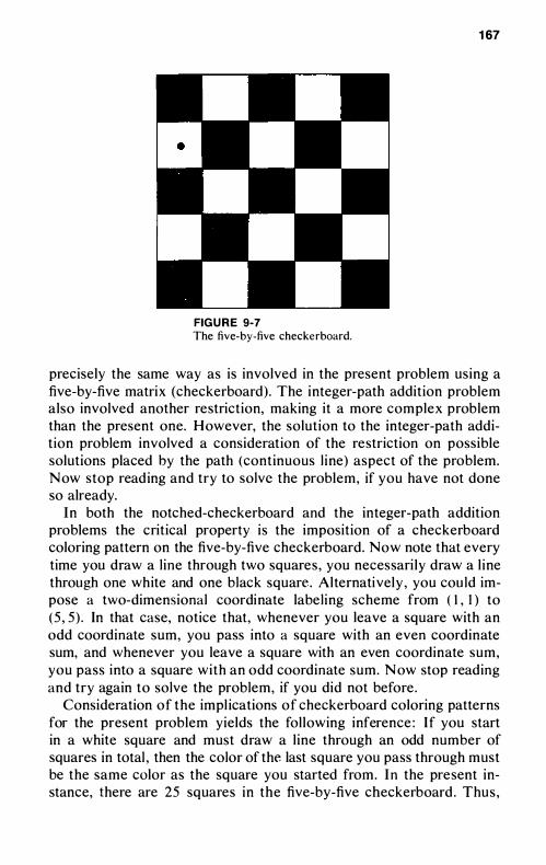
167

FIG U R E 9-7 The five-by-five checkerboard.

precisely the same way as is involved in the present problem using a five-by-five matrix (checkerboard) . The integer-path addition problem also involved another restriction, making it a more complex problem than the present one. However, the solution to the integer-path addi­tion problem involved a consideration of the restriction on possible solutions placed by the path (continuous l ine) aspect of the problem. Now stop reading and try to solve the problem, if you have not done so already.

In both the notched-checkerboard and the integer-path addition problems the critical property is the imposition of a checkerboard coloring pattern on the five-by-five checkerboard. Now note that every time you draw a l ine through two squares , you necessari ly draw a l ine through one white and one black square . Alternatively , you cou ld im­pose a two-dimensional coordinate label ing scheme from ( 1 , I ) to (5 , 5 ) . In that case, notice that, whenever you leave a square with an odd coordinate sum, you pass into a square with an even coordinate sum, and whenever you leave a square with an even coordinate sum, you pass into a square with an odd coordinate sum. N ow stop reading and try again to solve the problem, if you did not before .

Consideration of the impl ications of checkerboard coloring patterns for the present problem yields the fol lowing inference : I f you start in a white square and must draw a l ine through an odd number of squares in total , then the color of the last square you pass through must be the same color as the square you started from. In the present in­stance, there are 25 squares in the five-by-five checkerboard . Thus ,

168 Chapter 9

if you begin in a white square , you must end in a white square , and there must be exactly 1 3 white squares and 1 2 black squares in the checkerboard . However, in the checkerboard shown in Fig. 9-7 , there are 1 3 black squares and 1 2 white squares . Thus , starting from any white square on the board , it wil l be impossible to solve the problem of drawing a continuous l ine through each square once and only once.

SPECIAL CASE

Particularly in proof problems, it often happens that the theorem to be proved states a general relation that holds over a number of special cases or entities . In such problems, it is often useful to try to prove the theorem first for one or more of these special cases before an attempt is made to prove the theorem in general . The reason is that it is usually easier to prove the theorem for a special case than for the theorem in general . This argument is precisely the same one made for the advan­tages of posing and solving simpler problems in general . However, not all simpler problems are special cases of the problem you are try­ing to solve. The reverse, however, is almost invariably the case ­special cases are simpler problems than the general problem.

Proving a theorem true for one or more special cases increases the probability that the theorem is true in general , but unless you can prove the theorem true for all special cases , proving the theorem in a particular case does not, of course, prove the theorem in general .

However, disproving a special case of a conjectured theorem does di sprove the theorem in general . When you are uncertain about the truth of the theorem, it can be particularly useful to investigate the theorem in some special case, since a quick disproof of the theorem for the special case disproves the theorem in general. This exercise may save you considerable time that otherwise might be spent in fruitless attempts to prove a false theorem.

When the theorem is true, proving it true for one or more special cases may provide you with many of the elements needed in order to prove the theorem in general . This reason is perhaps the primary one for posing and solving special cases of general problems.

One use of the method of special case was discussed already in Chapter 6 on subgoals as a part of the method of mathematical induc­tion. Recall that, in the method of mathematical induction, we had to first prove the theorem true for n = 1 (a special case) and then show that if the theorem was true for n it was true for n + 1 . Thus , in proving that the sum of the first n integers equals n (n + 1 )/2 , we initial ly es­tablished that this was true for n = 1 .

Relations Belween Problems 169

Another use of the method of special case occurs sometimes in multiple-choice examination questions. For example, if you were asked to choose one of five formulas for the sum of the first n integers, the fastest method might be to investigate each formula on some special case, such as n = 5 , very l ikely determining that all but one of the answers produced a contradiction in that special case. Note that this is , in essence, a combination of the use of two problem-solving methods , namely, special case and the method of contradiction.

A similar problem often arises when you try to remember some formula you learned previously and think you recall it but are not sure . For example, in trying to recall the formula for the sum of the first n integers , you might erroneously recal l something such as n (n - 1 )/2. Such erroneous conjectures can easily be tested and re­jected by investigating their truth in one or more special cases . Since you often have a reasonably good idea of what the correct formula i s , a few rejections of incorrect statements of the formula wi l l usually be followed by a correct statement, which might simply be verified by mathematical induction.

Deriving a formula for the number of combinations of m things taken n at a time provides another good example of the use of the method of special case . U ndoubtedly you the reader have encoun­tered this formula in the past ; however, in my experience, many stu­dents fai l to remember the formula and most do not know how to derive it. Even if you do know how to solve the problem, it is useful to think of how you would go about applying the method of special case to derive the formula. Thus , consider the following:

Derive a formula for the number of combinations of m things taken n at a time (m > n) . Combinations refer to the number of different un­ordered sets of elements. That is , the set of two elements obtained by drawing X and then drawing Y is equivalent to the set obtained by draw­ing Y and then X. The set XYZ is equivalent to the set YXZ or the set ZYX. The ordering of the elements in the set is irrelevant. Furthermore, you are restricted to drawing an element only once from the underlying population of m elements. That is , you may sample from the underlying population n times without replacing the elements you sampled (sampling without replacement).

Stop reading and try to solve this problem, making use of the method of special case.

There are four specific aspects to the problem. F irst, there i s an underlying population of m elements. Second, you are picking a sample of n of these elements. Third , the sampling i s done without replace­ment; that is, every time you pick an element from the sample, you

170 Chapter 9

do not put it back in the population, so the population is reduced by one element every time you choose an element for the sample. Fourth, you are concerned with the number of different unordered sets ob­tained by this sampling procedure , rather than the number of different ordered sets .

Each of these four aspects could be changed to pose a problem related to the present one, some of them simpler than the present problem, which might faci litate its solution . If you have not yet solved the problem, stop reading and think how you might change one or more of the four aspects to derive a related problem or a special case that is simpler to solve than the original problem.

You could reduce the size of the underlying population of m ele­ments to, say, the special case of two elements. You would then also have to reduce the size of the sample to either one or two elements (n = 1 or 2). H owever, it is probably unnecessary to reduce both m and n in this way. It i s quite possible to leave m as it is and reduce the sample size to two e lements (n = 2) . You would now be considering the special case of the present problem where n = 2, namely, where one is selecting an unordered pair without replacement from the underlying population of m elements. Stop reading and try to solve the problem, if you have not done so already.

It wil l be easier to solve for the special case of the number of un­ordered pairs of elements if you consider the related problem of determining the number of ordered pairs of elements that can be selected from the population of m elements. This latter problem is quite trivial to solve : there are m ways to select the first e lement, and for each of these m ways, there are (m - 1) ways to select the second e lement ; thus , there are m (m - 1) ways to select an ordered pair of elements. Having determined the number of ordered pairs , it is quite possible to determine the number of unordered pairs . Stop reading and consider how you would do this , then generalize your answer to solve the original problem, if you have not done so already.

The critical difference between ordered and unordered pairs is that a pair of ordered elements XY is considered equivalent to the ordered pair YX, when unordered pairs are being considered . Thus , there are exactly two different ordered pairs of elements for each unordered pair. Knowing this , how can you solve the problem of determining the number of unordered pairs , if you know how many ordered pair there are? Stop reading and solve this problem and then generalize your answer to solve the original problem, if you have not done so already.

Clearly , if there are two ordered pairs for each unordered pai r and m (m - I ) ordered pairs , then there are m (m - I )/2 unordered pairs .

Relations Between Problem s 171

Now general ize this answer to the solution of the original problem, where you are selecting not a pair of e lements but a set of n elements at a time.

The relevant generalization of the solution to the special case is that the problem should be broken into two parts . First, the number of ordered sets of elements should be determined , then how many differ­ent orderings there are for each unordered set. Now use this analysis of the two subproblems to solve the original problem, if you have not done so already.

If you are not able immediately to general ize the solution of the special case to obtain a solution to the general case , then consider another special case, where n = 3. Here the number of ordered sets obtained by sampling without replacement i s m (m - I Hm - 2). The number of different orderings of each sample of three elements i s the number of permutations of three things. The number of permuta­tions of a set of three things is 3 . 2 . I , or 6, since there are three ways to pick the first element from the sample, two ways to pick the second , and one way to pick the th ird . Thus, the number of d ifferent unordered sets of three elements equals m (m - I Hm - 2)/3 . 2 . 1 = m(m - I Hm - 2)/3 ! . Stop reading and general ize the formula to the case of an unordered set of n elements, if you have not done so already.

Clearly, the general formula for the number of unordered sets of 11 elements selected from a population of m elements without replace­ment is m (m - I) . . . (m - n + I )/n ! = m !/n ! (m - n ) ! . The general principle for solving this problem comes from breaking it into two parts in order to determine, first, the number of ordered sets and , second , the number of distinct ways of ordering (reordering) the ele­ments in a particular ordered set (sample) . The number of unordered sets is equal to the number of ordered sets divided by the number of ways of ordering the e lements in a particular set. This general princi­ple is essential ly present in all special cases where n = 2 , 3, and so on. Thus , solving the problem for one or two special cases provides al l the essential ingredients for solving the problem in general .

The method of special case is also frequently usefu l in geometric problems. Consider the following proof problem in Eucl idean geometry :

You are given the fol lowing; (a) A straight l ine equal s an angle of 1 80°. (b) A right angle equals 90°. (c) If two paral lel l ines are cut by a trans­versal , the alternate interior angles are equal . Prove that the sum of the angles of any triangle equals 1 80°.

Stop reading and try to prove this theorem, making use of the method of special case.

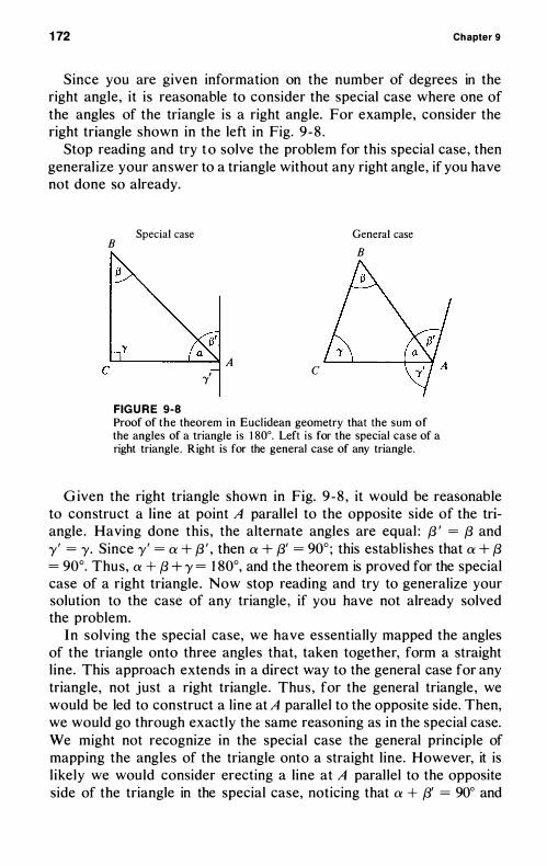
172 Chapter 9

Since you are given information on the number of degrees in the right angle, it is reasonable to consider the special case where one of the angles of the triangle is a right angle. For example, consider the right triangle shown in the left in Fig. 9 - 8 .

Stop reading and try to solve the problem for this special case , then general ize your answer to a triangle without any right angle, if you have not done so already.

B Special case General case

B

L..L. ___ --L._� A "'(' c

FIG U R E 9-8 Proof of the theorem in Eucl idean geometry that the sum of the angles of a triangle is 1 80°. Left i s for the special case of a right triangle. R ight is for the general case of any triangle .

G iven the right triangle shown in Fig. 9 - 8 , it would be reasonable to construct a line at point A parallel to the opposite side of the tri­angle . Having done this, the alternate angles are equal : f3 ' = f3 and y ' = y. Since y ' = ex + f3 ' , then ex + f3' = 90° ; this establ ishes that ex + f3 = 90°. Thus, ex + f3 + y = 1 80°, and the theorem is proved for the special case of a right triangle . Now stop reading and try to generalize your solution to the case of any triangle , if you have not already solved the problem.

In solving the special case, we have essentially mapped the angles of the triangle onto three angles that, taken together, form a straight l ine. This approach extends in a direct way to the general case for any triangle, not just a right triangle . Thus , for the general triangle , we would be led to construct a l ine at A parallel to the opposite side. Then, we would go through exactly the same reasoning as in the special case. We might not recognize in the special case the general principle of mapping the angles of the triangle onto a straight l ine. However, it is l ikely we would consider erecting a l ine at A paral lel to the opposite side of the triangle in the special case, noticing that ex + f3' = 90° and

Relations Between Problems 173

that f3 = f3 ' . This procedure includes the essential notion of construct­ing an additional line at A paral lel to the opposite side, and thus , you might think of the more general principle.

I n some instances, it turns out that proving the theorem for a small number of special cases constitutes the proof of the entire problem. Sometimes this result i s obvious in advance, and sometimes it only becomes obvious after considering a special case. For example , in Chapter 7 we considered the problem of proving that A 2 - A B + B2 > o. We considered the proof of this theorem only for the case where A > 0 and B > 0 but noted that the theorem was actually true for all A and B . Proving the theorem for a l l A and B essentially requires us to prove it for four cases : (a) A > 0 and B > 0; (b) A > 0 and B < 0; (c) A < 0 and B > 0 ; (d) A < 0 and B < O. The proof of the theorem for each of these four special cases involves breaking the problem up into three more special cases within each of the four previously mentioned special cases - namely, A > B, A = B, and A < B. Thus , in all , we have I 2 special cases for which to prove that A 2 - AB + B2 > 0 is true. But for each of these 1 2 special cases, the theorem is rather simple to prove.

An example in geometry where the general problem can be divided into two essential ly identical special cases i s provided by the proof of the following theorem:

You are g iven the fol lowing: (a) The measure of an intercepted arc i n degrees i s t he same as the measure of i t s corresponding central angle (namely, the angle determined by drawing the radi i from the center of the circle to the ends of the intercepted arc). (b) The sum of the angles of a triangle equals 1 80°. (c) The angles opposite the equal sides of an i sosceles triangle are equal . Prove that an angle inscribed in a circle has half as many degrees as i ts intercepted arc .

Stop reading and try to solve the problem by first considering a special case.

As is frequently true, there are many ways of formulating special cases of the present theorem. For example, we might consider the special case where the inscribed angle i s a right angle and try to prove that its intercepted arc i s 1 800 (that the cord for this arc i s a diameter of a circle) . Conversely, we might investigate the special case in which the intercepted arc was 1 80° and try to prove that the inscribed angle was 90°. Another type of special case would be to assume that the cords composing the inscribed angle were equal , and so on. We might consider many special cases before we hit on a special case that is

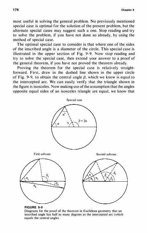
174 Chapter 9

most usefu l in solving the general problem. No previously mentioned special case is optimal for the solution of the present problem, but the alternate special cases may suggest such a one. Stop reading and try to solve the problem, if you have not done so already, by using the method of special case.

The optimal special case to consider is that where one of the sides of the inscribed angle is a diameter of the circle . This special case is i l l u strated in the upper section of Fig. 9 -9 . N ow stop reading and try to solve the special case , then extend your answer to a proof of the general theorem, if you have not proved the theorem already.

Proving the theorem for the special case is re latively straight­forward . First , draw in the dashed l ine shown in the upper circle of Fig. 9-9, to obtain the central angle {3 , which we know is equal to the intercepted arc . We can easi l y verify that the triangle shown in the figure is isosceles. N ow making use of the assumption that the angles opposite equal sides of an isosceles triangle are equal , we know that

Special case

First subcase Second subcase

FIG U R E 9-9 Diagrams for the proof of the theorem in Eucl idean geometry that an in scribed angle has half as many degrees as the intercepted arc (which equal s the central angle).

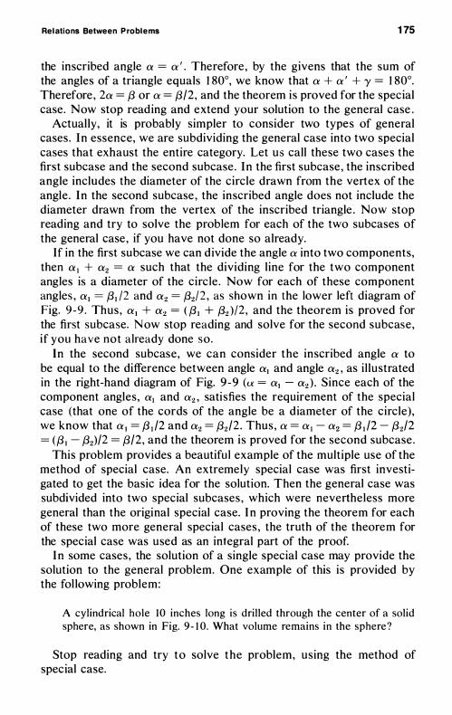
Relations Between Problems 175

the inscribed angle a = a ' . Therefore , by the givens that the sum of the angles of a triangle equals 1 80°, we know that a + a ' + '}' = 1 80°. Therefore , 2a = f3 or a = f3/2, and the theorem is proved for the special case. Now stop reading and extend your solution to the general case .

Actual ly, it is probably simpler to consider two types of general cases . In essence, we are subdividing the general case into two special cases that exhaust the entire category. Let us call these two cases the first subcase and the second subcase . In the first subcase , the inscribed angle includes the diameter of the circle drawn from the vertex of the angle . In the second subcase , the inscribed angle does not include the diameter drawn from the vertex of the inscribed triangle . Now stop reading and try to solve the problem for each of the two subcases of the general case , if you have not done so already.

If in the first subcase we can d ivide the angle a into two components, then a l + a2 = a such that the dividing l ine for the two component angles is a diameter of the circ le . Now for each of these component angles , a1 = f31 /2 and a2 = f32/2 , as shown in the lower left diagram of Fig. 9 -9 . Thus , al + a2 = ( f3 1 + f32 )/2 , and the theorem is proved for the first subcase. N ow stop reading and solve for the second subcase, if you have not already done so.

In the second subcase, we can consider the inscribed angle a to be equal to the difference between angle al and angle a2 , as i l lustrated in the right-hand diagram of Fig. 9 -9 (u = al - a2 ) ' Since each of the component angles, al and a2 ' satisfies the requirement of the special case (that one of the cords of the angle be a d iameter of the circle) , we know that a l = f3 1 /2 and a2 = f32/2 . Thus , a = al - a2 = f3 1 /2 - f32/2 = (f3 1 - f32)/2 = f3/2, and the theorem is proved for the second subcase .

This problem provides a beautifu l example of the multiple use of the method of special case. An extremely special case was first investi­gated to get the basic idea for the solution. Then the general case was subdivided into two special subcases , which were nevertheless more general than the original special case. I n proving the theorem for each of these two more general special cases , the truth of the theorem for the special case was used as an integral part of the proof.

I n some cases, the solution of a single special case may provide the solution to the general problem. One example of this is provided by the fol lowing problem:

A cylindrical hole 10 inches long i s drilled through the center of a solid sphere, as shown in Fig. 9 - 1 0 . What volume remains in the sphere?

Stop reading and try to solve the problem, using the method of special case.

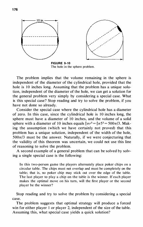
176

I�-- 1 0 in. --..-I

FIG U R E 9- 1 0 The hole i n the sphere problem.

The problem implies that the volume remaining in the sphere is independent of the d iameter of the cylindrical hole, provided that the hole is 1 0 inches long. Assuming that the problem has a unique solu­tion, independent of the diameter of the hole, we can get a solution for the general problem very simply by considering a special case . What is this special case? Stop reading and try to solve the problem, if you have not done so already.

Consider the special case where the cylindrical hole has a diameter of zero. I n this case, since the cyl indrical hole is 1 0 inches long, the sphere must have a diameter of 1 0 inches, and the volume of a solid sphere with a diameter of I O inches equals t7Tr3 = t7T53 = 5007T/3 . Mak­ing the assumption (which we have certain ly not proved) that this problem has a unique solution , independent of the width of the hole, 5007T/3 must be the answer. Natural ly, if we were conjecturing that the validity of this theorem was uncertain, we could not use this line of reasoning to solve the problem.

A second example of a general problem that can be solved by solv­ing a single special case is the following:

I n this two-person game the players alternately place poker chips on a circular table . The chips must not overlap and must be completely on the table ; that is , no poker chip may stick out over the edge of the table. The last player to play a chip on the table is the winner. I f each player makes the optimal move on h is turn , will the first player or the second player be the winner?

Stop reading and try to solve the problem by considering a special case.

The problem suggests that optimal strategy wil l produce a forced win for either player I or player 2, independent of the size of the table. Assuming this , what special case yields a quick solution?

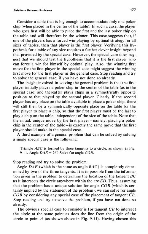
Relations Between Problem s 177

Consider a table that is big enough to accommodate only one poker chip (when placed in the center of the table) . In such a case, the player who goes first will be able to place the first and the last poker chip on the table and wil l therefore be the winner. This case suggests that, if one of the players has a forced win playing by optimal strategy for all sizes of tables, then that player is the first player. Verifying this hy­pothesis for a table of any size requires a further clever insight beyond that provided by the special case. However, the special case does sug­gest that we should test the hypothesis that it is the first player who can force a win for himself by optimal play. Also, the winning first move for the first player in the special case might suggest the winning first move for the first player in the general case. Stop reading and try to solve the general case, if you have not done so already.

The insight involved in solving the general problem is that the first player initial ly places a poker chip in the center of the table (as in the special case) and thereafter plays chips in a symmetrical ly opposite position to that played by the second player. Clearly, if the second player has any place on the table available to place a poker chip, there will sti l l then be a symmetrically opposite place on the table for the first player to place a chip, so that the first player must be the last to play a chip on the table, independent of the size of the table . Note that the initial , unique move by the first player - namely, placing a poker chip in the center of the table - is exactly the same move that the first player should make in the special case.

A third example of a general problem that can be solved by solving a single special case is the following :

Triangle A B C is formed by three tangents to a circle, as shown in Fig. 9 - 1 1 . Angle DA E = 26°. Solve for angle COB.

Stop reading and try to solve the problem. Angle DA E (which is the same as angle BA C ) is completely deter­

mined by two of the three tangents. It is impossible from the informa­tion given in the problem to determine the location of the tangent BC as it intersects the circle anywhere within the arc ED. Thus, assuming that the problem has a unique solution for angle COB (which i s cer­tainly implied by the statement of the problem) , we can solve for angle CO B by considering any special case of the placement of tangent C B. Stop reading and try to solve the problem, if you have not done so already.

The obvious special case to consider is for tangent CB to intersect the circle at the same point as does the line from the origin of the circle to point A (as shown above in Fig. 9 - 1 1 ) . Having chosen this

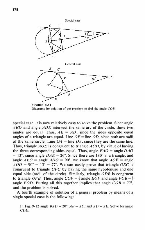
178

Special case

General case

E

�-;�------�-- A

FIG U R E 9-1 1 Diagrams for solution of the problem to find the angle COB.

special case, it is now relatively easy to solve the problem. Since angle A ED and angle A D E intersect the same arc of the circle, these two angles are equal . Thus, A E = AD, since the sides opposite equal angles of a triangle are equal . Line OE = line OD, since both are radi i of the same circle . Line OA = l ine OA , since they are the same l ine . Thus , triangle A OE is congruent to triangle A OD, by virtue of having the three corresponding sides equal. Thus , angle EA 0 = angle DA 0 = 1 3 ° , since angle DA E = 26°. Since there are 1 80° in a triangle , and angle A EO = angle ADO = 90°, we know that angle A OE = angle A OD = 90° - 1 3° = 77°. We can easily prove that triangle OEC is congruent to triangle OFC by having the same hypotenuse and one equal side (radi i of the circle) . Similarly, triangle ODB i s congruent to triangle OFB. Thus , angle COF = i angle EOF and angle FOB = i angle FOD. Putting all this together implies that angle COB = 77°, and the problem is solved.

A fourth example of solution of a general problem by means of a single special case is the following :

I n Fig. 9 - 1 2 angle BA D = 20°, A B = A C, and A D = A E. Solve for angle CDE.

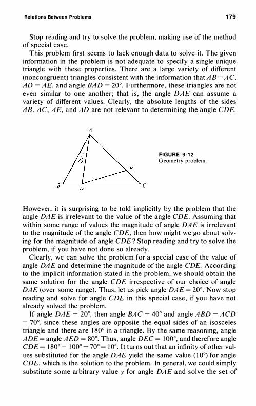
Relations Between Problems 179

Stop reading and try to solve the problem, making use of the method of special case.

This problem first seems to lack enough data to solve it . The given information in the problem is not adequate to specify a single unique triangle with these properties. There are a large variety of different (noncongruent) triangles consistent with the information that A B = A C, AD = A E, and angle BA D = 20°. Furthermore , these triangles are not even similar to one another; that i s , the angle DA E can assume a variety of different values. Clearly, the absolute lengths of the sides A B. A C, A E, and AD are not re levant to determining the angle CDE.

A

B'---........ ::......-----........ C

FIG U R E 9- 1 2 G eometry problem.

However, it i s surpris ing to be told implicitly by the problem that the angle DA E is irrelevant to the value of the angle CDE. Assuming that within some range of values the magnitude of angle DA E is irrelevant to the magnitude of the angle CDE, then how might we go about solv­ing for the magnitude of angle CDE ? Stop reading and try to solve the problem, if you have not done so al ready.

Clearly, we can solve the problem for a special case of the value of angle DA E and determine the magnitude of the angle CDE. According to the implicit information stated in the problem, we should obtain the same solution for the angle CDE irrespective of our choice of angle DA E (over some range) . Thus , let us pick angle DA E = 20°. Now stop reading and solve for angle CDE in this special case , if you have not already solved the problem.

If angle DA E = 20°, then angle BA C = 40° and angle A BD = A CD = 70°, since these angles are opposite the equal sides of an i sosceles triangle and there are 1 80° in a triangle . By the same reasoning, angle A DE = angle A ED = 80°. Thus , angle DEC = 1 00°, and therefore angle C DE = 1 80° - 1 00° - 70° = 1 0°. I t turns out that an infinity of other val­ues substituted for the angle DA E yield the same value ( 1 0°) for angle CDE, which i s the solution to the problem. In general , we could simply substitute some arbitrary value y for angle DA E and solve the set of

180 Chapter 9

equations to determine the value of angle CDE in a manner that would be independent of y. H owever, it i s considerably simpler to solve the problem by choosing a single special case, since the given information implies that the solution to the spec ial case is equ ivalent to the solu­t ion to the general problem.

GENERALIZATION

Just as it is sometimes useful to solve a special case prior to working on a more general problem, it is also frequently useful to do the opposite and generalize the problem somewhat.

G eneralization plays a role in problem solving in at least three different ways . First, as a necessary part of problem solving, we usually abstract from a problem certain properties belonging to a more general class of problems and thus relevant for determining the pre­viously establi shed principles needed for solving our present problem. Second , after we have solved the problem, it i s often useful to consider whether we could generalize a solution from it to a wider class of prob­lems in order to derive a more general conclusion or one or more corol­laries of the principle establi shed in the problem we just solved . Third , occasional ly (though in my experience not too frequently) , it may be useful to pose and attempt to solve a more general problem prior to working on the current problem, even when the solution to that more general problem is not yet known to us .

The first role that generalization plays in problem solving has really already been discussed in Chapter 3 in connection with the representa­tion of information. Recall that a critical aspect of solving many problems consists in retrieving from memory the relevant previously establi shed relations and principles with common properties needed to solve the present problem.

It may be that the current problem is real ly a special case of a general class of problems for which we already know a simple rule for solution. For example, if the present problem is the linear equation 2x + 5 = 1 3 , we know that the solution to this particular l inear equation can be achieved by using the general methods for solving any linear equation of the form ax + b = c . Similarly, if the equation were a quadratic of the form 7x2 + 2x - 4 = 0, we have a formula for solving any equation of the form ax2 + bx + c = O. A broad range of higher order equations can be solved by certain types of numerical methods . If we have a par­ticular equation that fal l s within the scope of a numerical method , we know we can apply this method to solve the particular problem.

In a geometric context, if a problem gives two sides of a right tri-

Relations Between Problems 181

angle and we are asked to solve for the third side, we know a general method that is applicable to solving all such problems - namely, use of the Pythagorean Theorem, ('2 = a2 + b2•

If we are given a problem in which we must determine the number of combinations of seven things taken four at a time, we need only retrieve the formula for the number of combinations of m things taken n at a time and substitute in the appropriate values for m and n in order to solve the problem.

Ordinari ly, to solve problems we must combine use of more than one previous ly establ i shed principle. Thus, in all proof problems, whether algebraic , geometric , or logical , the proof invariably requires a sequential application of several previous ly establ i shed principles. In a story-algebra problem, first the methods of representing the in­formation algebraical ly must be applied , then the methods appropriate for solving whatever algebraic equations are derived from the story.

The examples of general ization in this most important context could be extended indefinitely. Suffice it to say that, in this sense, general iza­tion plays an enormously important role in problem solving. H owever, as discussed in Chapter 3 , this use of the method of generalization depends critical ly on the degree of understanding you have of the pre­viously establi shed principles in the areas relevant to the current prob­lem. A few general principles regarding representation of information are discussed in Chapter 3 and Chapter 1 0 ; however, the field i s just too vast and thus is outside the scope of this book.

The second role of generalization in problem solving has l itt le use for a student in a course but is frequently valuable for a mathematician or scientist solving a new problem to see if the solution can be generalized to a larger class of problems. A long the same line, we may try to derive some additional consequences as relatively straightforward corollaries of the solution to the present problem. For example , if we had estab­l i shed that the two diagonals of a rectangle were equal , we might ask whether this result could be general ized to a larger class of situations. It would then be relatively straightforward to notice that the solution generalizes to d iagonals connecting equal and paral lel sides of any polygon, includ ing regular hexagons or octagons and parallelograms .

Another example in a geometric context i s provided by the theorem that the alternate interior angles formed by a transversal intersecting two parallel lines are equal. This result easi ly generalizes to establ ish that the other pair of alternate interior angles are equal and that both pairs of corresponding exterior angles are equal as wel l .

A final example, again in a geometric context : Assume that we have already establ ished that an inscribed angle has half as many degrees as its intercepted arc . From this result it i s relatively trivial to show

182 Chapter 9

that the angle formed by a tangent and a chord meeting it at the point of contact has also half as many degrees as its intercepted arc. In fact, the latter theorem could be thought of as simply being a l imiting case of the former theorem.

The third possible role of generalization in problem solving is , in a sense, the inverse of the previously described role of the method of special case ; namely, it might facil itate solution of a specific problem to formulate a more general problem that had not been previously solved. Then we might either solve the more general problem or, in any event, work on the solution of the more general problem for a time, before going back to working on the specific problem.

Polya ( 1 957 , pp. 1 08- 1 09) argues that this problem-solving technique is quite useful and he gives the following example :

The problem is to find a plane that passes through a given line and bisects the volume of a given octahedron.

Polya asserts that i t would be useful to formulate the more general problem of finding a plane that passes through a straight line and bisects the volume of any solid with a center of symmetry. The solution to this problem is fairly obvious, namely, a plane determined by the given l ine and the center of the solid with a center of symmetry. Since an octahedron is a special case of a solid with a center of symmetry, the original, specific problem is solved. Polya asserts that the value in formulating the more general previously unsolved problem is that it can focus the problem solver's attention on the necessary properties in the original problem that must be used in order to solve it. As Polya himself points out, however, the primary function of generalization was in the formulation of the more general problem. If we had generalized the problem in an inappropriate way - that i s , using some property that was not in fact central to the solution of the original problem ­then the formulation of the general problem would l ikely have been of no help and might even have been a hindrance in the solution of the original problem.

A two-dimensional analog of the previous example would be to deter­mine the line that passes through a given point and, say, a given square b isecting the volume of that square . A generalization of this problem would be to determine a l ine that passed through a given point and bisected the area of a given plane-figure with a center of symmetry. Again, formulating the more general problem directly suggests the solution - namely, that the line passes through the given point and the center of symmetry of the figure .

Relations Between Problem s 183

Personal ly, I am somewhat skeptical of the alleged benefits of try­ing to solve a more general problem, when the solution to the more general problem is not known to the problem solver. However, I am sure that thinking of possible generalizations of the current problem does often aid the problem solver in realizing all of the properties of the problem, some of which may be the critical properties in order to solve the problem. In this sense, the alleged third role of generaliza­tion is very similar to the first role of thinking of generalizations of the problem when the solution of the more general problems is already known. I t is a question of representing the important properties or principles that are present in a special problem, and , to do so, an abstraction process is involved . Abstracting the properties from a problem is , in essence, generalization. Thus , once again we see that the role of generalization and the role of representation of information (as discu ssed in Chapters 3 and 1 0) are very closely l inked and perhaps identical .

10

To pics in

Mathematical Representatiof'

As stated in Chapter 2 , problems contain information concerning givens, actions, and goal s . The first and most basic step in problem solving is to represent this information in either symbolic or d iagram­matic form. Symbolic form refers to the expression of information in words , letters, numbers , mathematical symbols , symbolic logic nota­tion, and so on. Diagrammatic form refers to the expression of in­formation by a collection of points, l ines, angles, figures , directed lines (vectors) , matrices, plots of functions , graphs , and the l ike. Often the same information should be represented using a variety of symbolic or d iagrammatic notations . In fact, diagrammatic representation is general ly labeled ; for example, points, l ines, and cells in a matrix have symbols attached to them in the d iagram. Of course, problems are stated originally in some form, often relying heavily upon verbal lan­guage . The first step in solving such a problem is to translate from the representation given explic itly or implicitly in the original state­ment of the problem to a more adequate representation.

Topics in Mathematical Representation 185

This chapter is concerned with selected topics in the mathematical or precise representation of information in problems. Although precise representation of the information in a problem is the first step to take in trying to solve a problem, I deferred discussing this important topic to this late chapter of the book for two reasons .

First, although some general statements can be made about the representation of information in a large variety of problems, most of the principles of representation are specific to particular problem areas. Effective representation for problems from some area of mathematics , science , or engineering depends upon knowing centuries of conceptual development in the relevant areas of mathematics , science , and en­gineering. I doubt that mankind will ever develop a general method for determining what are the useful concepts to define in any particular area. Certainly, no such general principles of how to define good con­cepts are presented in this book. The best I can do i s to present those types of concepts and the principles for representing them that have proved the most useful in a wide variety of areas of formal problem solving. This is what is done in the present chapter, without any claim to completeness (which would be preposterous) and with only minimal claim to logical organization of the concepts and the principles of mathematical representation.

Second , although some of the principles of mathematical representa­tion are reasonably simple and can be communicated to even the most minimal ly prepared student, some of the principles discussed in the latter half of this chapter are concerned with concepts from various areas of mathematics with which some readers wi l l be unfamiliar. I hope that these readers will profit from the sections on sets, relations, operations , mappings, functions, and real-valued functions of a real variable. However, it seemed wisest to put this material near the end of the book so as not to discourage readers with less mathematical sophistication .

The material in the latter portion of this chapter is real l y a brief, simple discussion of selected mathematical topics , l argely modern algebra and combinatorial mathematics . This material i s primari l y intended for students who have some background in these topics i n col lege, high school , o r grade school new math courses. For such stu­dents, these sections are intended as review of the relation of certain mathematical concepts to the general methods of problem solving dis­cussed in this book. For students with no background in set theory, modern algebra, and combinatorial mathematics , these sections may be rather hard going and require considerable study. Such students should consult regu lar mathematics books concerned with these topics ,

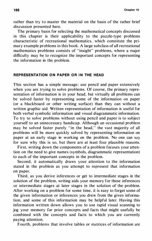
186 Chapter 1 0

rather than try to master the material on the basis of the rather brief discussion presented here .

The primary basis for selecting the mathematical concepts discussed in this chapter is their appl icabi l ity to the puzzle-type problems characteri stic of recreational mathematics , which constitute the pri­mary example problems in this book. A large subclass of all recreational mathematics problems consists of " insight" problems, where a major difficulty may be to recognize the important concepts for representing the information in the problem.

REPRESENTATION ON PAPER OR IN THE HEAD

This section has a simple message : use pencil and paper extensively when you are trying to solve problems. Of course , the primary repre­sentation of information is in your head , but virtual ly all problems can be solved faster by representing some of the information on paper (or a blackboard or other writing surface) than they can without a written graphic aid. Written representation of information is useful for both verbal symbolic information and visual diagrammatic information. To try to solve problems without using pencil and paper is to subject yourself to an unnecessary handicap. Although an occasional problem may be solved faster pure ly " in the head ," the vast majority of al l problems wi l l be more quickly solved by representing information on paper at an earl y stage in working on the problem. No one can say for sure why this i s so, but there are at least four plausible reasons.

First, writing down the components of a problem focuses your atten­tion on the need to give names (symbols , diagrammatic representation) to each of the important concepts in the problem.

Second , it automatical ly draws your attention to the information stated in the problem as you attempt to represent that information on paper.

Third , as you derive inferences or get to intermediate stages in the solution of the problem, writing aids your memory for these inferences or intermediate stages at later stages in the solution of the problem. After working on a problem for some time , it i s easy to forget some of the given information or inferences you drew from the given informa­tion, and some of th is information may be helpful later. Having this information written down allows you to use rapid visual scanning to jog your memory for prior concepts and facts that might useful ly be combined with the concepts and facts to which you are currently paying attention.

Fourth , problems that involve tables or matrices of information are

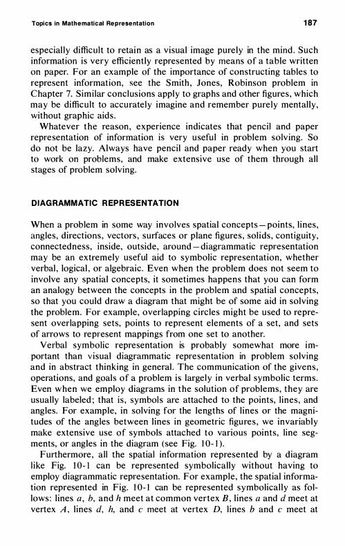
Topics in Mathematical Representation 187

especial ly difficu l t to retain as a visual image purely in the mind . Such information is very efficiently represented by means of a table written on paper. For an example of the importance of constructing tables to represent information, see the Smith , Jones, Robinson problem in Chapter 7. Similar conclusions apply to graphs and other figures, which may be difficult to accurately imagine and remember pure ly mental ly, without graphic aids .

Whatever the reason, experience indicates that pencil and paper representation of information is very useful in problem solving. So do not be lazy. Always have pencil and paper ready when you start to work on problems, and make extensive use of them through all stages of problem solving.

DIAGRAMMATIC REPRESENTATION

When a problem in some way involves spatial concepts - points, l ines, angles, directions , vectors , surfaces or plane figures , sol ids , contiguity, connectedness, inside, outside, around - diagrammatic representation may be an extremely useful aid to symbolic representation, whether verbal , logical , or algebraic. Even when the problem does not seem to involve any spatial concepts, it sometimes happens that you can form an analogy between the concepts in the problem and spatial concepts, so that you could draw a diagram that might be of some aid in solving the problem. For example, overlapping circ les might be used to repre­sent overlapping sets, points to represent elements of a set, and sets of arrows to represent mappings from one set to another.

Verbal symbolic representation is probably somewhat more im­portant than visual diagrammatic representation in problem solving and in abstract thinking in general . The communication of the givens , operations, and goals of a problem is largely in verbal symbolic terms. Even when we employ diagrams in the solution of problems, they are usually labeled ; that is , symbol s are attached to the points, l ines , and angles. For example, in solving for the lengths of l ines or the magni­tudes of the angles between l ines in geometric figures , we invariably make extensive use of symbols attached to various points, l ine seg­ments, or angles in the diagram (see Fig. 1 0- 1 ) .

Furthermore , al l the spatial information represented by a diagram l ike Fig. 1 0- 1 can be represented symbolically without having to employ diagrammatic representation. For example, the spatial informa­tion represented in Fig. 1 0- 1 can be represented symbolical ly as fol­lows : l ines a , b, and h meet at common vertex B , l ines a and d meet at vertex A , l ines d, h, and c meet at vertex D, l ines b and c meet at

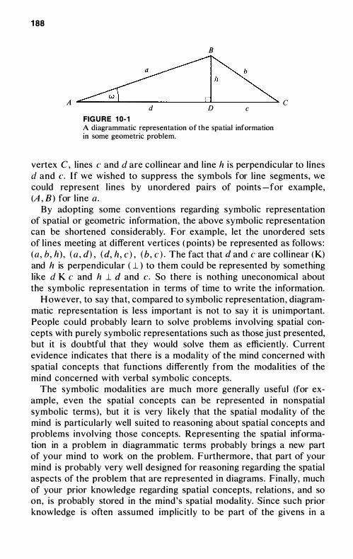
1 88

B

� A d D c

C FIG U R E 1 0- 1 A diagrammatic representation o f t h e spatial information in some geometric problem.

vertex C, lines c and d are col l inear and line h is perpendicular to l ines d and c. I f we wished to suppress the symbols for line segments, we could represent l ines by unordered pairs of points -for example, (A , B ) for l ine a.

By adopting some conventions regarding symbolic representation of spatial or geometric information, the above symbolic representation can be shortened considerably. For example, let the unordered sets of l ines meeting at different vertices ( points) be represented as follows : (a , b , h ) , ( a , d) , (d, h , c ) , ( b , c ) . The fact that d and c are coll inear (K) and h is perpendicular ( -L ) to them could be represented by something like d K c and h -L d and c. So there is noth ing uneconomical about the symbolic representation in terms of time to write the information.

H owever, to say that, compared to symbolic representation , diagram­matic representation is less important is not to say it is unimportant. People could probably learn to solve problems involving spatial con­cepts with purely symbolic representations such as those just presented, but it is doubtful that they would solve them as efficiently. Current evidence indicates that there is a modality of the mind concerned with spatial concepts that functions differently from the modal ities of the mind concerned with verbal symbolic concepts.

The symbolic modalit ies are much more generally useful (for ex­ample, even the spatial concepts can be represented in nonspatial symbolic terms), but it is very l ikely that the spatial modality of the mind is particularly well suited to reasoning about spatial concepts and problems involving those concepts. Representing the spatial informa­tion in a problem in diagrammatic terms probably brings a new part of your mind to work on the problem. Furthermore, that part of your mind i s probably very well designed for reasoning regarding the spatial aspects of the problem that are represented in diagrams. Finally, much of your prior knowledge regarding spatial concepts, relations , and so on, is probably stored in the mind 's spatial modality. Since such prior knowledge is often assumed implicit ly to be part of the givens in a

Topics in Mathematical Representation 189

problem, it is c learly important that you have access to your memory for such information.

SYMBOLIC REPRESENTATION

General Principles of Concept Representation

The simplest and most frequent step in symbolic representation of the information in problems is to choose some symbol (or sequence of sym­bols) to stand for a concept. The concept represented by a symbol can be anything the human mind can conceive. Let us take the symbol x and examine a few of the many concepts it can represent in various prob­lems. The symbol x can represent any real number or it can repre­sent a particular, but (in the present problem state) unknown, real number. Al ternatively , x can range over the integers ( . . . , -2 , - 1 , 0, I , 2, . . . ), positive integers, negative integers , rationals , irration­als , complex numbers (y + zi), the elements of some set, subsets of three elements from some given larger set, and so on. The symbol x can be the label of a particular point, l ine, or figure in a geometric problem, the label of some particular element in a practical construction problem (such as a gate , a piece of a fence, or a stump), or one of the tokens in a puzzle or game (such as ticktacktoe) .

Any symbol can be used to represent any concept, subject to one and only one restriction: the same symbol should almost never be used to represent two concepts that are not known to be equivalent through­out the present problem. There are many other principles of effective representation of concepts, but we can violate them without the ri sk of producing conc lus ions that contradict the given information in the problem. We cannot represent by the same symbol two concepts that are not equivalent in a problem, without running a substantial risk of generating contradictions to the given information and deriving incorrect answers.

By contrast, it i s perfectly safe to use different symbol s for concepts or quantities that may later prove to be equivalent or equal . H owever, it reduces the load on the memory, if you notice such equivalences or equal ities before you assign symbols to concepts or quantities , and assign the same symbol to concepts that must be equivalent. Never­theless, in view of the grave danger involved in mistakenly using the same symbol for nonequivalent concepts, it is best to always use different symbols for d ifferent concepts , unless you are absolutely certain that the concepts are equivalent throughout the problem.

190 Chapter 1 0

Mnemonics and Symbol Conventions

Although you may use any symbol you l ike to represent any concept, subject to the above-mentioned restriction, people tend to develop habits regarding the types of symbol s used for different types of con­cepts. For example, in mathematics , i , j, k , I, m , and n tend to be used for variables that range over the integers ; u, v, w, x, y , and z tend to be used for variables that range over real numbers ; p and q are usual ly used for probabilities (ranging over the real numbers between 0 and 1 ) ; and f, g , and h tend to b e used primari ly to represent unknown functions.

In scientific and engineering problems, symbols chosen to represent different concepts tend to have some easy mnemonic relation to a longer name for the concept in verbal language, usual ly being the first letter of the name (or the first letter of the key word , if the name of the concept is some phrase containing several words) . For example, f and F might be used for forces, A for area, p and P for pressures, t and T for times, r and R for rates, and w and W for work. Other sym­bolic naming conventions in science and engineering may be purely arbitrary, such as using G reek letters (8 , a , f3) for angles ; but adhering to such conventions (whether mnemonic or arbitrary) makes it easy to remember in any particular problem what concepts the symbols repre­sent. Maintaining consistency across different problems in the types of symbols you use to represent types of concepts brings long-term memory to the aid of short-term memory in recal l ing what is meant by each symbol you are using in any problem.

Single Symbols

If ease of remembering what a symbol represents is so important for efficient problem solving, why not use two or three letters from the ful l name or even the ful l name for the concept? Something l ike this is occasional ly done in problems where the names of two or more con­cepts have the same first letter ; for example, using to for total, te for tension, and ti for time, when all three concept names appear in some problem. This sort of multi symbol naming of a concept is useful in some cases, and these cases will be discussed in subsequent sections on the use of subscripts , vectors , and functions. However, in cases where the mnemonic advantages of using several symbols to represent a single concept are the only advantages , this practice is almost always a mistake . U nless there are a very large number of concept names that all have the same first letter, it is always possible to think of different single symbols to represent each concept, such that each symbol has an adequate mnemonic relation to the concept name so abbreviated .

Topics in Mathematical Representation 191

For instance, you could use some letter in the name other than the first, capital letters as well as small letters (for example, T and t), corre­sponding Greek letters (for example, T for t) , phonetical ly s imilar letter names if you know phonetics (for example, d for t), or change the con­cept name to some functional synonym (for this problem) that starts with a different first letter (for example , sum for totalJorce for tension, duration for time) .

For the purposes of unique representation in any one problem, it is unnecessary to represent concepts by a string of several symbols (as we do in verbal language) , because so few different concepts are in­volved in any given problem. You do want to maintain a strong mne­monic relation between your chosen symbol and the concept name it abbreviates, because that provides you with access to the information stored in your long-term memory concerning the concept and its pre­viou sly establ ished relations to other concepts. H owever, we have just seen that a single symbol is u sual l y adequate to accomplish this rela­tion without a lot of table lookup.

This being the case, there are substantial cognitive advantages to using single symbols to represent concepts in problem solving. It is fair to say that psychology does not know for sure the exact reasons why this is so, but the experience of problem solvers establ ishes that it is easier to work with single-symbol names for concepts . Many plausible reasons can be given. Single symbol s probably place less of a load on short-term and long-term verbal and visual memory. So, for example, it is easier to remember the visual image or verbal statement of an expression, formula, or equation that uses single symbols for each concept than one which uses more symbol s to represent each concept. Single symbols take less time to write on paper and generally have less potential for erroneous writing or reading.

Expressions

To reduce the cognitive and memory load in solving problems, you can also reduce the number of different symbols used to represent con­cepts by recognizing the relations between concepts right away when you are deciding upon representation . For example, if John i s 30 pounds heavier than Bi l l , let b represent Bi l l ' s weight and let b + 30 represent John's weight, to avoid assigning any new symbol at all to represent John' s weight. This use of expressions involving a small number of symbols to represent all the concepts in the problem can speed up the solution to the problem by immediately reducing the number of un­knowns to those having only nontrivial relations to one another. However, it must be recognized that you are performing two steps at

192 Chapter 1 0

once : representing the concepts in the problem and expressing some relatively simple relations between concepts. Trying to do these two steps at once increases the probabil ity of error, though when per­formed successful ly, it usually al lows you to solve the problem faster. My advice is to try to combine these two steps and use expressions to represent concepts. H owever, if you find yourself making lots of errors, go back to the more compulsive and systematic procedure of first assigning symbols to all different and important concepts in the prob­lem, and only then start expressing the relations between these con­cepts - for example, by equations such as j = b + 30, where j represents John 's weight.

Subscripts

I n a problem with many different quantities of the same type - such as many different t imes , rates , d istances, volumes, heights, or radi i of circular bases - it is often desirable to use two-symbol codes for representing these concepts. In these problems, the type of concept can be thought of as a property of some object, activity, or object­performing-an-activity. One of the two symbols in the two-symbol code is used to represent the property and the other symbol to represent the object, activity, or object-performing-an-activity. In addition, the mnemonic convention i s that the property is represented by the main symbol, with the object, activity, or object-performing-an-activity represented by a subscript. So, for example, the height of cyl inder A could be represented by hA and the radius of its base by rA ' Similarly, hB and rB could be used for cylinder B , and so on.

Subscripts usually appear to the right and somewhat below the main symbol, but they occasional ly appear to the lower left of the main sym­bol . So long as there are no exponents involved in solving a problem, you can use superscripts for the second symbol just as well as sub­scripts. Superscripts can appear to the upper left or upper right. How­every, since there is very frequently a danger that superscripts will be confused with exponents, it is good practice to avoid using them.

The only possible excuse for using a superscript occurs in problems where the objects to which a property appl ies are differentiated along two or more d imensions, and the values of the various dimension are completely noncomparable. For example, imagine that in some prob­lem you have various complex containers, each of which has several component containers with different shapes and dimensions. Container A might be composed of a cyl indrical subcontainer, two cubical sub­containers, and a rectangular subcontainer. There are also complex

Topics in Mathematical Representation 193

containers B and C, each composed of subcontainers. How should you represent the volume of each subcontainer in container A , for example? For ease in remembering what symbols represent what and the associated ease in retrieving formulas for volumes from your long­term memory, you might try using a notation such as the following: Let V/ be the volume of the cyl indrical subcontainer of A ; let 1 V,A be the volume of the first cubical ( square base) subcontainer of A ; let

2V,A be the volume of the second cubical subcontainer of A ; let vt be the volume of the rectangular subcontainer of A .

You encounter notations l ike the above, with both left and right subscripts and a superscript (or even two !) , but I think they are poor notations. Superscripts are dangerous because they can be confused with exponents . If a superscript is put to the upper left of the main symbol , it el iminates the possibil ity of it being confused with an ex­ponent for the main symbol ; but it is then apt to be mistaken for an exponent for the symbol to the left in a multiplication problem (for example, hA Vr for "h times A V/ ' ) . If you are always careful to put the entire three- or four-symbol complex into parentheses - for example, (2 Vf ) - you will avoid these confusions. However, you wil l then have a complex symbol with as many as six component symbols ; indeed, even four component symbols are too many.

In cases l ike the above, you should probably scrap the entire effort and use a single letter for each concept or, at most, a two-symbol code for each concept. If you can easi ly think of some single symbol s that have some reasonably good mnemonic relation to the concepts they represent, use such symbols . Or, fail ing this , make an arbitrary assignment of single symbols to concepts and write down the assign­ment in a table or diagram, for consulting when necessary. The time saved in the repeated writing of the symbols in various statements or equations usually more than compensates for the extra time spent in table or diagram lookup. Furthermore , it is rather hard to visualize, verbalize, or otherwise think about such complex symbols as the ones in the above example.

Multiple Subscripts

One important exception to the above advice regarding complex sym­bols are cases where you have an entire matrix (two-dimensional or higher dimensional) of objects or activities , each entry of which has one or more properties . In such cases , use multiple subscripts (possibly separated by commas), all on the lower right of the main symbol (for example, XUk or xu.d. Such cases ari se frequently in statistics , where

194 Chapter 1 0

X;ik might represent the wheat yield on the kth plot of land , subjected to the ith value on one treatment d imension (for example, the amount of some kind of ferti l izer), and subjected to the jth value on another treat­ment d imension (for example, the amount of water) .

Why i s use of a complex symbol with multiple subscripts recom­mended in the stati stics example and not in the previous example? I n the stati stics example there are a number of dimensions, and every combination of values on every d imension (that is, every entry in the matrix) has a defined value of the property in question (for instance, wheat yield) . I n the problem concerning volumes of complex containers, every complex container could have different shapes of subcontainers and d ifferent numbers of each shape. Suppose you defined dimensions l ike the "shape of a subcontainer" ; the complex container to which the subcontainer belonged ; and whether it was the first, second, and so on, subcontainer of this shape to be a part of the complex container. You would then have lots of cel ls in the matrix with no objects corre­sponding to them in the problem (empty cel ls in the matrix) . This is more trouble than it i s worth.

When you actual ly have a large number of objects in some multi­dimensional matrix , there is real ly no feasible alternative to using multiple subscripts. Furthermore , in matrix problems l ike the statistics example, we often do operations such as summing over all the entries in some row or column without ever having to look up in any table or diagram the meaning of each complex symbol. When subscript notation i s used, a convenient notation exists for indicating sums or products ­for instance :

and

Subscript notation i s always indicated in problems where multiple sums or products of this type are l ikely to be used in the solution. Where such multiple sums and products or some other computations or relations involving the subscripts are not likely to appear anywhere in the solution, it is questionable whether you should ever use a sym­bol with more than one subscript.

Example Problem

Tom, Dick, and H arry mow lawns in the summer to earn money. They each have a lawn mower, and one Saturday they decide to mow a 5 ,900 square foot lawn together, us ing all three lawn mowers. Tom mows 70 square feet per minute, Dick 50, and H arry 40. Dick and Harry start mowing the lawn at the same t ime, but Tom has trouble start ing h is mower and is delayed for 30 minutes. All three boys stop mowing at the same t ime, when the lawn is finished. How long does Tom mow?

Topics in Mathematical Representation 195

I n solv ing this problem, the principal step is to represent the informa­tion in algebraic notation and set up the equations . After this , the se­quence of algebraic actions (operations) i s trivial . Stop reading, and represent the information in this problem, using the principles dis­cu ssed in this chapter ; then solve the problem.

There are several steps involved in representing the information, and you should be aware of them, even though you may be able to solve such problems quickly and easi ly. The same types of steps are involved in all story-algebra problems, and similar representational steps are involved in many other types of problems as wel l .

First we have to represent the unknown quantities for which we are to solve. Here that means having some expressions represent (stand for) the times that Tom, Dick, and H arry work. It is economical and an aid to visual and verbal memory to choose a single symbol (often a letter) to stand for an unknown quantity. You may choose any sym­bols you l ike for the unknown quantities represented , provided that you do not use the same symbol to represent quantities that might not be equal .

It is perfectly safe to use different symbols for quantities that may later prove to be equal . However, it aids the memory, if you notice such equal ities before you assign symbols to quantities and assign the same symbol to quantities that must be equal . For example, in the present problem, we can use t for the time that Dick mowed and al so for the time that Harry mowed. We know that these times are equal since Dick and Harry start and stop at the same time . It would place an unnecessary strain on the memory to use to , t l , and t2 to stand for the mowing times of Tom, Dick, and H arry, respectively, though there is no mathematical reason why numerical subscripts cannot be used for these purely nominal or naming purposes.

Note that there i s a good mathematical reason for not choosing to represent Tom's mowing time by the symbol 8, because al l number symbols , including 8, are already implicitly given as concepts in a story-algebra problem, and Tom's mowing time i s not known to be equal to 8. This sort of objection does not apply to the use of numbers in a purely nominal way in subscripts , and , of course, nominal numerical subscripts are used frequently in mathematics, science, and engineer­ing. Often the problem gives only the names "first force" or " second force," and in such cases the obvious representation is it and h .

I n problems with many unknown quantities, i t i s desirable, for the same reason of minimizing the load on human memory, to choose let­ters that have easy mnemonic relations to the fu l l names of the quanti­ties represented . For example, we choose t or T for time quantities and r or R for rate quantities. If there are many different quantities of

196 Chapter 1 0

the same type, such as several different times, then i t may be best to represent them by a two-symbol code, such as tT, tn , and tH , where the t indicates a time and the subscript indicates which time. The subscript should also have some easy mnemonic relation to the ful l name of the quantity represented . In the present problem, we might initial ly have chosen tT, tn , and til to stand for the times that Tom, Dick, and H arry mow, though, as already noted , this is unnecessary.

Now here is the solution. This is a simple work-rate problem. The primary equation to use in such problems is that work equals the sum of all the rate times time components. In this problem, that means setting up an equation such as

where

70(t - 30) + SOt + 40t = 5 ,900

t = time Dick and Harry mow t-30 = time Tom mows

Solving the above equation gives t = 50, and therefore Tom mows for 20 minutes .

SOME IMPORTANT MATHEMATICAL CONCEPTS

Ordered and Unordered Pairs

Ordered pairs without replacement Each of the possible permutations of m things taken two at a time is just another name for an ordered pair of elements (i,j ) , such that both i and j are members of the set of m things and i and j are not the same thing or element of the set. This is sampling twice from a set of m elements without replacement of the element already sampled. Ordered pairs of this type ( permutations) are frequently involved in problems.

For example , consider a problem in which some group has the ritual of everyone kissing everyone else on the forehead , and you are sup­posed to determine the number of people in the group from the number of kisses or vice versa. Kissing on the forehead is represented by an ordered pair of persons in which the first member of the pair is the kisser and the second member is the person kissed. Having recognized that this is an ordered pair (permutation) problem, you can solve the problem in a manner similar to the way you solved other problems ­namely, by determining how many ways there are to fill each position in the ordered pair. I n this problem, there are m ways to fill the first position, and , with it fil led, there are m - 1 ways to fill the second

Topics In Mathematical Representation 197

position. Hence, there are m ( m - I ) ways to fil l both positions (with different elements). Thus , the m persons exchange m ( m - 1 ) forehead kisses. Of course , to determine m from m ( m - 1 ) , you have to solve a quadratic equation , but in the average problem of this type , that would be very simple.

Ordered pairs with replacement A known or unknown point in a plane is often best represented by an ordered pair of symbols repre­senting its distances from each of two (usual ly perpendicular) axes, though , of course, in many problems a point can be represented by just a single symbol such as A or a dot on a page . However, frequently the representation of a point in a plane should be by an ordered pair of symbols - an ordered pair of numbers for a known point, an ordered pair of letters for an unknown point. S ince the values of the two coordi­nates can be equal , the representation of a point in a plane by an ordered pair is an example of sampling twice with replacement from the entire population of coordinate values (whether finite or infinite). Sampl ing with replacement means that when you have chosen the value for the first coordinate , you put that value back into the population so that it can be drawn again as the value for the second coordinate . Thus , if there were m possible coordinate values, there would be m2 possible points - that is, m2 ordered pairs of coordinate values.

Unordered pairs without replacement Although forehead kisses are represented by ordered pairs of persons, l ip kisses (assuming mutual kissing ) are represented by unordered pairs. That i s , if A kisses B, B is assumed also to be kissing A. Thus, there i s no basis for distin­gu ishing between (A , B ) and ( B , A ) .

This is a combinations problem rather than a permutations problem. As we discussed in Chapter 9 , the number of combinations of m things taken two at a time i s m (m - 1 ) /2 . We derived this figure by reasoning as follows : The number of permutations is m ( m - 1 ) , and there are two permutations for every combination (two ordered pairs for each unordered pair). Thus , we should divide the number of ordered pairs (permutations) by 2 to get the number of unordered pairs (combinations) .

A l ine segment i s determined by its two end points . Often a l ine (segment) wi l l be defined as an unordered pair of (distinct) points, with every different unordered pair of points in the total set of points repre­senting a different l ine. Notice that a l ine is indeed an unordered pair of points, not an ordered pair, in most cases . H owever, it is perfectly possible to have directed l ine segments in a problem (that is, l ines with arrows on one end , or vectors), in which case the l ine (A , B ) i s different

198 Chapter 1 0

from the l ine (B, A ) , where A and B are two different points in the set of points.

The above two examples of unordered pairs are instances of un­ordered pairs where the sampling is without replacement. A person is not assumed to be able to kiss himself on the l ips . A l ine segment is determined by two end points that are distinct, that is , two different points.

Unordered pairs with replacement We can also obtain unordered pairs by sampling from a population with replacement. An example might be the di stinct combinations obtained by throwing two dice, which might produce these results : 6-6, 6 - 5 , 6-4, 6- 3 , 6-2 , 6- 1 , 5 - 5 , 5 - 4, . . . , 2-2 , 2- 1 , I - \ . T o compute the number of distinguishable throws of two dice, we reason that the order of the two dice is not important and thus 6 - 5 is the same outcome as 5 - 6.

Offhand you might think that the number of unordered pairs obtained by sampling with replacement would be equal to the number of ordered pairs sampling with replacement divided by 2, as was the case for sampl ing without replacement (permutations and combinations). How­ever, this is not the case. Most of the unordered pairs of outcomes obtained by sampling with replacement do indeed have two distinct ordered-pair counterparts, but there is a subset of the unordered pairs each of which has only a single ordered-pair counterpart. These latter pairs are 6 -6 , 5 - 5 , 4 -4 , 3 - 3 , 2-2 , and I - \ .

I n general , if you are sampling with replacement two times from a population of m elements, the number of different unordered pairs will be

+ m2 - m _ m (m + 1 ) m

2 - 2

This result is obtained by reasoning as follows : exactly m of the un­ordered pairs are of the form i-i, where i = 1 , . . . , m . The remaining m2 - m ordered pairs have exactly two ordered-pair counterparts for each unordered pair. Thus, the quantity ( m2 - m ) should be divided by 2 to get the number of unordered pairs, and m should be added to this total to get the total number of different unordered pairs.

Systematic listing of unordered pairs Occasional l y we need to l ist all the unordered pairs that can be obtained by sampling, either with or without replacement, from some population. The efficient way to accomplish such a l i sting is to put al l of the elements in the population into an ordering, whether they have any natural ordering or not. Having

TOpics In Mathematical Representation 199

ordered the elements from 1 to m, we can then l ist all of the unordered pairs by proceeding as fol lows: If the unordered pairs are being ob­tained by sampling with replacement, we take each element from the popu lation and pair it with itself and every element below it in the ordering. Thus , we would obtain pairs such as 5 - 5 , 5 - 4, 5 - 3 , 5 -2 , 5 - 1 , 4- 4, 4-3 , 4-2 , 4 - 1 , 3 - 3 , 3 -2 , 3 - 1 , 2-2, 2 - 1 , I - I . I f the unordered pairs are being obtained by sampling without replacement, we take each element in the population and pair it with each of the elements below it in the ordering. Thus , we would have li stings such as 5 - 4, 5 - 3 , 5 -2 , 5 - 1 , 4 -3 , 4-2, 4 - 1 , 3 -2 , 3 - 1 , 2 - 1 .

Importance of ordered and unordered pairs Ordered and unordered pairs are very common concepts in problems, and you should be alert for the possibility of representing concepts as ordered or unordered pairs of other concepts, frequently an important step in solving the problem. In a sense, this representation involves your recognizing a relation between different concepts and incorporating that relation into your representation of concepts in the problem, which is similar to representing concepts by expressions, as we discussed previously. You should also be careful to note whether the ordered and unordered pairs are being obtained with or without replacement, for, as stated earl ier, it makes a considerable difference in the number of such pairs.

Often you wil l real ize that some concept can be represented by a pair of other concepts before you real ize whether the pair should be considered an ordered pair or an unordered pair and whether the sampling is with or without replacement. H owever, by being explicitly aware of the di stinctions, you wil l try to decide whether the pair is ordered or unordered and whether the sampling i s with or without replacement, before trying to use the concept in solving the problem.

Ordered and Unordered Sets

Ordered and unordered pairs generalize easi ly to ordered and unor­dered sets of elements greater than two. So we can have an ordered or unordered set of three elements (A , E, C ) , four elements ( w , x, Y, z ) , and so on.

Ordered sets without replacement Each permutation of m things taken n at a time (n < m ) is an ordered set of n elements. I n getting any particular permutation, we are sampling n times without replacement from a set of m elements. Thus , there are m possible ways to fil l the first position (m possible elements that could be selected first ) , (m - I )

200 Chapter 1 0

ways to fil l the second position, . . . , and ( m - n + I ) ways to fi l l the n th ( last) position, or m ( m - I ) . . . (m - n + I ) = m !/ ( m - n ) ! different ways to select all n elements (assuming all m elements are dis­tinct) . An example of a permutation problem (ordered sets, sampling without replacement) is as follows :

A gym teacher wi shes to put on a balancing demonstration in which one of the stunts wi l l be to have four boys stand on each others shoulders in a s ingle tower. Out of the class of 20 boys, the gym teacher wishes to select the most stable tower of four boys. To do th is he plans to try each possible tower of four boys once and time how long they are able to balance successful ly on each others shoulders without fal l ing over. How many such towers of four boys must the gym teacher investigate?

Stop reading and try to solve the problem. Since there are 20 boys in the gym class and a tower of four boys

constitutes an ordered set of four elements sampled from the class without replacement, this is a permutations problem. Therefore , the number of possible towers is 20 !/(20 - 4) ! = 20 !/ 1 6 ! .

Ordered sets with replacement A point or vector in n-dimensional space can be represented by an ordered set of its n coordinates (Xl

' X2 , • • • , xn ) . Such an ordered set of n elements is obtained by sampling with replacement from a population of, say, m possible coordinate values exactly n times . The number of possible ordered sets obtained by sampling n times from a population of m elements is equal to m n .

Unordered sets without replacement A triangle is an unordered set of three different points ( sampling three times without replacement from the set of all points). A quadrilateral is an unordered set of four different points in a plane . Each combination of m things taken n at a time (n < m ) is an unordered set of elements such that none of the elements is identical ly the same element (for example, one is sampling n times without replacement from a set of m elements). The number of combinations of m thi ngs taken n at a t ime is simply the number of permutations of m things taken n at a time , divided by the number of different permutations for the same combination of n elements. Since there are n ! different permutations for each combination of n elements, there are m !1 [n ! (m - n) !] combinations of m things taken n at a time. An example of a combinations problem is as fol lows:

How many different bridge hands ( 1 3 cards) can be obtained by deal ing 1 3 cards out of a standard 52-card deck?

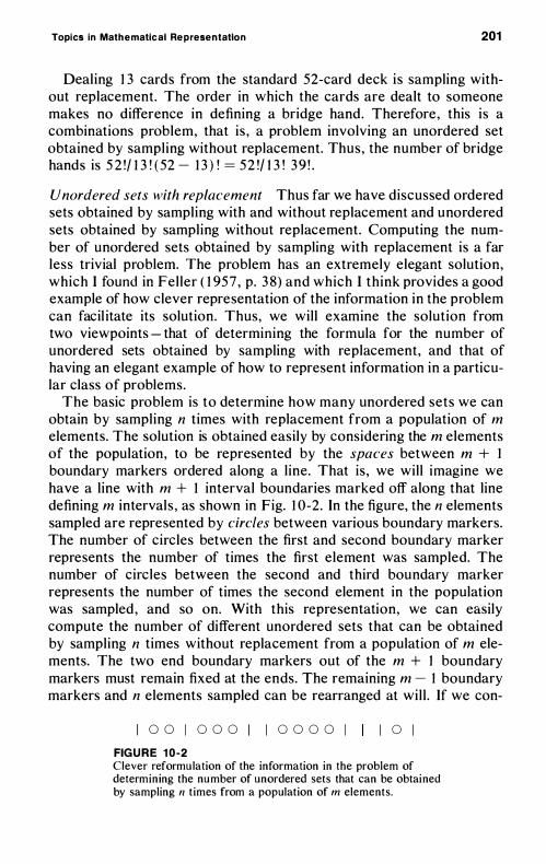
Topics in Mathematical Representation 201

Dealing 1 3 cards from the standard 52-card deck i s sampling with­out replacement. The order in which the cards are dealt to someone makes no difference in defining a bridge hand . Therefore , this is a combinations problem, that is , a problem involving an unordered set obtained by sampling without replacement. Thus, the number of bridge hands is 5 2 !/ 1 3 ! ( 52 - 1 3 ) ! = 52 !/ 1 3 ! 3 9 ! .

Unordered sets with replacement Thus far we have discussed ordered sets obtained by sampling with and without replacement and unordered sets obtained by sampling without replacement. Computing the num­ber of unordered sets obtained by sampling with replacement is a far less trivial problem. The problem has an extremely elegant solution, which I found in Fel ler ( 1 957 , p. 3 8) and which I think provides a good example of how clever representation of the information in the problem can facil itate its solution. Thus, we wil l examine the solution from two viewpoints - that of determining the formula for the number of unordered sets obtained by sampling with replacement, and that of having an elegant example of how to represent information in a particu­lar class of problems.

The basic problem is to determine how many unordered sets we can obtain by sampling n times with replacement from a population of m elements. The solution is obtained easily by considering the m elements of the population, to be represented by the spaces between m + 1 boundary markers ordered along a l ine. That is , we wil l imagine we have a line with m + 1 interval boundaries marked off along that line defining m intervals , as shown in Fig. 1 0-2 . In the figure, the n elements sampled are represented by circles between various boundary markers. The number of circles between the first and second boundary marker represents the number of times the first element was sampled. The number of circles between the second and third boundary marker represents the number of times the second element in the population was sampled , and so on. With this representation, we can easily compute the number of different unordered sets that can be obtained by sampling n times without replacement from a population of m ele­ments. The two end boundary markers out of the m + 1 boundary markers must remain fixed at the ends. The remaining m - 1 boundary markers and n elements sampled can be rearranged at wil l . If we con-

1 0 0 I 0 0 0 I 1 0 0 0 0 I FIG U R E 1 0 -2

1 0 1

Clever reformu lation of the information in the problem of determining the nu mber of unordered sets that can be obtained by sampling n times from a population of m elements.

202 Chapter 1 0

sider any particular rearrangement to be obtained by sampling n times without replacement from the population of n + m - I elements, then the number of such rearrangements of the l ines and circles i s easi ly determined , namely, ( n + m - 1 ) !In ! (m - 1 ) ! .

Thus , we have transformed the problem of sampling n times with replacement from a population of m elements to the problem of sam­pl ing n times without replacement from a population of n + m - 1 ele­ments. In both cases , we are trying to compute the number of unordered sets obtained by such a sampling. S ince we know the solution to the problem of obtaining the number of unordered sets obtained by sampl ing without replacement (combinations), we now know the answer to the problem of determining the number of unordered sets obtained by sampling with replacement.

Relations

Relations are labeled connections between concepts. Examples of relational concepts include, among others : father of, brother of, sibl ing of, descendant of, prior to , less than , equal to , identical to, heavier than , older than , beside, includes, is a member of. Relations can be written as "a R b" (meaning perhaps "a is the father of b" ) or as R (a , b ) . I n the latter case, R ( a , b ) is true (equals I ) , if and only if the relation R obtains for the ordered pair ( a , b ) , and R ( a , b ) is false (equal s zero), if and only if the relation R does not obtain for the ordered pair ( a , b ) .

Relations can be classified according to whether they satisfy cer­tain properties (axioms). For example, a relation can be reflexive (a R a, for all a in some set ) , antireflexive (a not-R a, for all a in some set), or neither. Relations can be symmetric or commutative (a R b implies b R a , for all a and b in some set ) , anti symmetric (a R b im­pl ies b not-R a, for all a and b in some set) , or neither. Relations can be transitive (a R b and b R c imply a R c, for all a, b, and c in some set ) or not. Relations that are reflexive, symmetric , and transitive form an especial ly important class of relations known as equivalence rela tions. " Equal to " and "identical to" are equivalence relations, but so are "has the same weight as," "is the same color as," and "is just as good as . "

Some students find i t difficult to distinguish the concepts of equiva­lence, equality, and identity, and indeed the meanings of these concepts are somewhat variable, especial ly in going from science to mathematics. To get an idea of why we sometimes need to distinguish them, consider the fol lowing examples.

Suppose you were thinking about your prospects for immortal ity, and you imagined that it might be possible to form a complete duplicate of

Topics in Mathematical Representation 203

yourself that was the same configuration of molecules as yourself but, of course, used different molecules. Such a duplicate would be equal to you in every respect, but the duplicate would not be identical to you , since the two of you in fact would be two different parts of the universe. I dentical twins are considered to be genetical ly equal , but they are not identical , since they are two different entities . All the molecules of some class are considered to be equal, but since there is more than one such molecule in each class, the molecules of a given class are not identical . A thing is identical only to itself, but it can be equal to all duplicates . Of course, many people fee! that it is l ikely that no two entities can be exact duplicates in every respect, but this is not too important for the definition of equal ity. We can simply say that two things are equal, if there i s no property that we can currently determine to distinguish them (except of course the fact that they are not the identical ly same entity).

Two entities may be equivalent to each other in some one respect (one property) without being equal to each other (equivalent to each other in all respects). This is pretty obvious when it is put this way. Two girl s can have the same weight (to the nearest pound ) , have the same shooting percentage in basketbal l , have the same number of points on a test, and so on. Thus , it i s clear that (a) two names of ob­jects that are identical ly the same real ly refer to the same object, (b) two names of objects that are equal refer to two different objects that are equivalent in all respects, and (c) two names of objects that are equiva­lent in some respect are not necessari ly identical or equal in all respects.

Sometimes there is no need to distinguish all three types of "same­ness" concepts. For example, in real-variable mathematics, where a symbol has only one property, its numerical value, there is no need to distinguish equivalence and equality. Furthermore , our definition of identity is not quite the same intuitively as it is when we discuss objects presumed to exist in the real world . In mathematics not viewed as applying to the real world, two expressions are identical ly equal ( == ) , if and only if they have the same values across all substitutions for free variables (for example, x2 - 1 == [x + 1 ] [x - 1 ] ) . Two expres­sions are often said to be equal (=) if and only if they have the same values for at least one substitution for free variables (for example , x2 + 2 = 6 for the substitution x = 2 ) .

Operations

I n Chapter 2 , operations were contrasted with givens . I ntuitively, operations were the things that you could do to change the state of the problem and givens were the materials you had to work with (the

204 Chapter 1 0

starting point or initial problem state) . You could attach a symbol to each operation that you could perform to change the problem state , but what would that accomplish? For one thing, it might allow you more conveniently to list the alternative actions that could be per­formed at each node in the state-action tree. However, this is not the primary reason for attaching symbols to operations.

The primary reason for using a symbol to represent an operation is that you can formulate problems in which the givens are composed of statements that involve action concepts as well as object or property concepts. Consider a problem to solve two l inear equations in the variables x and y for the values of x and y -for example, 2x + y = I and x - 6y = 20. Addition, subtraction, and multiplication operations are indicated in each of these statements, but the particular actions they indicate (for example, multiply y by 6) are not the actions you take in solving the problem. The actions you take are to add , subtract, multiply, or divide both sides of some equation by the same quantity and to substitute equals for equals .

By contrast , these are problems in which you might take the opera­tions of addit ion, subtraction , multipl ication , and so on, of two quanti­ties as the operations used at various nodes of the state-action tree. For example, water-jar problems (such as the one discussed in Chapter 8) involve presenting several jars that hold different quantities of l iquid. One is asked to produce some quantity of liquid that is different from the capacity of any jar. The method of solution involves, in es­sence, adding and subtracting the capacities of each of the jars.

I magine that you have a five-quart jar and a three-quart jar and are attempting to obtain exactly one quart of water. You could fill the three­quart jar, pour it into the five-quart jar, fill the three-quart jar, pour two quarts into the five-quart jar, and have exactly one quart left in the three-quart jar, as required.

In water-jar problems, adding and subtracting quantities are the operations in the state-action tree. In solving equations, adding and subtracting quantities are operations used in constructing statements ; adding and subtracting the same quantities to both sides of an equation are operations in the state-action tree. Perhaps there should be two different names to distinguish operations at these two different levels in a problem. In any event, it i s important for clear thinking to keep operations at the two levels distinct in your mind.

Mappings and Functions

I magine that you have the elements of some set A (the argument set), the elements of another set T (the target set), and a set of arrows, each

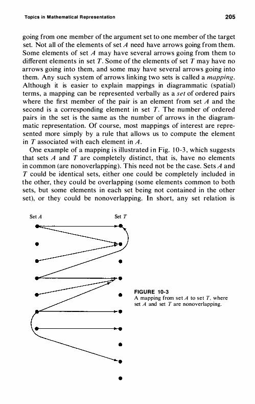
TOpics in Mathematical R epresentation 205

going from one member of the argument set to one member of the target set. Not all of the elements of set A need have arrows going from them. Some elements of set A may have several arrows going from them to different elements in set T. Some of the elements of set T may have no arrows going into them, and some may have several arrows going into them. Any such system of arrows l inking two sets is called a mapping. Although it is easier to explain mappings in diagrammatic (spatial ) terms, a mapping can be represented verbal ly as a set of ordered pairs where the first member of the pair i s an element from set A and the second i s a corresponding element in set T. The number of ordered pairs in the set is the same as the number of arrows in the diagram­matic representation. Of course, most mappings of interest are repre­sented more simply by a rule that allows us to compute the element in T associated with each element in A .

One example of a mapping i s i l lustrated i n Fig. 1 0 -3 , which suggests that sets A and T are completely d istinct, that is, have no elements in common (are nonoverlapping) . This need not be the case. Sets A and T could be identical sets, either one could be completely included in the other, they could be overlapping (some elements common to both sets, but some elements in each set being not contained in the other set), or they could be nonoverlapping. In short, any set relation is

Set A Set T

•

FIG U R E 1 0-3 A mapping from set A to set T. where set A and set T are nonoverlapping .

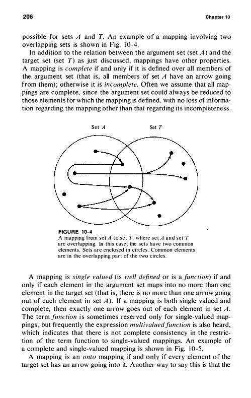
206 Chapter 1 0

possible for sets A and T. An example of a mapping involving two overlapping sets is shown in Fig. 1 0 -4.

I n addition to the relation between the argument set ( set A ) and the target set (set T) as just discussed , mappings have other properties. A mapping i s complete if and only if it is defined over al l members of the argument set (that i s , all members of set A have an arrow going from them) ; otherwise it is incomplete. Often we assume that all map­pings are complete, since the argument set could always be reduced to those elements for which the mapping is defined , with no loss of informa­tion regarding the mapping other than that regarding its incompleteness.

Set A Set T

FIG U R E 1 0-4 A mapping from set A to set T. where set A and set T are overlapping. In this case , the sets have two common elements. Sets are enclosed in c irc les . Common elements are in the overlapping part of the two circles .

A mapping i s single valued ( is well defined or is a function) if and only if each element in the argument set maps into no more than one element in the target set (that i s , there is no more than one arrow going out of each element in set A ) . If a mapping is both single valued and complete, then exactly one arrow goes out of each element in set A . The term function i s sometimes reserved only for single-valued map­pings, but frequently the expression multivalued function is also heard, which indicates that there i s not complete consistency in the restric­tion of the term function to single-valued mappings. An example of a complete and single-valued mapping is shown in Fig. 1 0 -5 .

A mapping i s an onto mapping i f and on ly i f every element of the target set has an arrow going into it. Another way to say this is that the

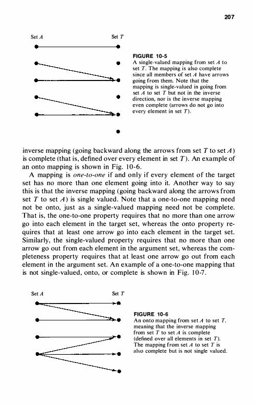
Set A Set T • •

�:

�: •

207

FIG U R E 1 0-5 A single-valued mapping from set A to set T. The mapping i s also complete s ince all members of set A have arrows going from them. Note that the mapping is single-valued in going from set A to set T but not in the inverse direction, nor is the inverse mapping even complete (arrows do not go into every element in set T) .

inverse mapping (going backward along the arrows from set T to set A ) is complete (that i s , defined over every element in set T ) . An example of an onto mapping is shown in Fig. 1 0-6 .

A mapping is one-lo-one i f and on ly i f every element of the target set has no more than one element going into it. Another way to say this is that the inverse mapping (going backward along the arrows from set T to set A ) is single valued . Note that a one-to-one mapping need not be onto, just as a single-valued mapping need not be complete. That is , the one-to-one property requires that no more than one arrow go into each element in the target set, whereas the onto property re­quires that at least one arrow go into each element in the target set. Similarly, the single-valued property requires that no more than one arrow go out from each element in the argument set, whereas the com­pleteness property requires that at least one arrow go out from each element in the argument set. An example of a one-to-one mapping that is not single-valued , onto, or complete is shown in Fig. 1 0 -7 .

Set A Set T

FIG U R E 1 0-6 An onto mapping from set A to set T, meaning that the inverse mapping from set T to set A is complete (defined over al l elements in set T). The mapping from set A to set T is also complete but is not single valued.

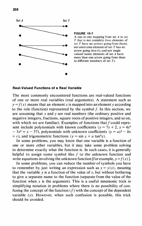
208

Set A Set T

•

FIGURE 1 0-7 A one-Io-one mapping from set A to set T thaI is not complete (two elements of sel T have no arrows going from them). not onto (one element of set T has no arrow going into i t ) . and not single valued (some elements of set A have more than one arrow going from them to d ifferent members of set T) .

Real-Valued Functions of a Real Variable

The most commonly encountered functions are real-valued functions of one or more real variables (real arguments) . A statement such as y = f(x) means that an element x i s mapped into an element y according to the ru le (function) represented by the symbol f. I n thi s section , we are assuming that x and y are real numbers (the ordinary positive and negative integers, fractions, square roots of positive integers, and so on, with which we are famil iar) . Examples of functions that f could repre­sent include polynomials with known coefficients (y = 7x + 2, y = 4r

- 3x2 + X - 37) , polynomial s with unknown coefficients (y = art - bx

+ c), and trigonometric functions (y = sin x + a tan3x) . I n some problems, you may know that one variable is a function of

one or more other variables, but it may take some problem solving to determine exactly what the function is. In such cases, it is generally helpful to assign some symbol l ike f to the unknown function and write equations involving the unknown function [for example, y = f(x) ] .

I n some problems, you can reduce the number of symbols you have to remember by just writing an expression such as y = y (x) , meaning that the variable y is a function of the value of x, but without bothering to give a separate name to the function (separate from the value of the function when x is the argument). This is a useful mnemonic trick in simpl ifying notation in problems where there i s no possibi l ity of con­fusing the concept of the function (f) with the concept of the dependent variable (y) . However, when such confusion is possible, this trick should be avoided .

1 1

Problems from Mathematics,

Science, and Engineering

This chapter is designed to establ ish the general ity of the problem­solving methods discussed throughout the book. In previous chapters, the problems used to i l lustrate the methods were deliberately selected so that they could be solved by the reader with no more background than a high school student with one year of algebra and one year of plane geometry. Many of the problems were of the puzzle (or brain teaser or recreational mathematics) variety, which require no special­ized knowledge of mathematics , science, or engineering. Although methods for solving such problems have some recreational interest, there is also a serious practical reason in mastering them, for they are also useful for solving serious problems in all areas of mathematics , science, and engineering. This chapter is designed to demonstrate this appl icabil ity and to give the reader some experience in it .

ALGEBRA

The solution of systems of simultaneous l inear equations provides a simple example of the u se of evaluation functions, hi l l c l imbing, and

210 Chapter 1 1

subgoal s . As a n example, consider the following system of three l inear equations :

or

2x + y - 3z = 1

x + 2y + 5z = 9

3x - 3y - IOz = 4

(E l )

(E2)

(E3)

The operations available for solv ing such a system are essential ly the fol lowing. We can (a) multiply both sides of an equation by the same num­ber, (b) add equal s to equal s (or subtract equal s from equals) , and (c) sub­stitute equal s for equal s . As an example of the first, consider the action of mult iplying both sides of equation (E2) by the number -2 . This yields the equation -2x - 4y - lOz = - 1 8. As an example of the second operation, consider the action of adding the equation just derived from (E2) to (E 1 ) :

2x + y - 3z =

-2x - 4y - lOz = -1 8

- 3y - 1 3z = -17

3y + 1 3z = 1 7

(E l )

( -2) . (E2)

(E4)

As an example of the third operation, consider the fol lowing substitution of an expression for x, derived from (E2), into (E I ) :

x = -2y - 5 z + 9

2 (-2y - 5z + 9) + y - 3z = 1

(E2)

(E l )

I f we were given a particular numerical value for x, we could, of course, also substitute that part icular value for x anywhere it appeared in any equat ion. The goal i s to derive three expressions of the form x = __ ,

y = __ , and z = __ , where specific numbers appear in the blanks.

Now stop reading and try to solve the problem. The solution of such a problem involves primari ly the use of an

evaluation function and the subgoal method, with perhaps a l ittle use of hi l l c l imbing. The evaluation function i s concerned with the number of variables (unknowns) in each equation and the number of indepen­dent equations involving any particular set of variables (unknowns). The original system of equations consists of three equations, each of which has three variables (unknowns). From this starting point, a more highly valued state would be one in which we had two equations involving the same two unknowns. An even more highly valued state would be one in which we had one equation involving one unknown. Still more highly valued would be a state in which we had two equa­tions, each of which involved a different, single unknown. The most

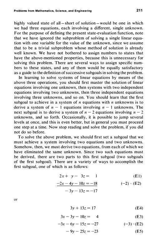
Problems from Mathematics, Science, and Engineering 2 1 1

highly valued state of all - short of solution - would be one in which we had three equations , each involving a different, s ingle unknown. For the purpose of defining the present state-evaluation function, note that we have ignored the subproblem of solving a single l inear equa­tion with one variable for the value of the unknown, since we assume that to be a trivial subproblem whose method of solution i s already well known. We have not bothered to assign numbers to states that have the above-mentioned properties, because this is unnecessary for solv ing this problem. There are several ways to assign specific num­bers to these states , and any of them would be equal ly sati sfactory as a guide to the definition of successive subgoals in solving the problem.

In learning to solve systems of l inear equations by means of the above three operations , you should first master the solution of l inear equations involving one unknown , then systems with two independent equations involving two unknowns, then three independent equations involving three unknowns , and so on. You should learn that the first subgoal to achieve in a system of n equations with n unknowns i s to derive a system of n - I equations involving n - I unknowns. The next subgoal i s to derive a system of n - 2 equations involving n - 2 unknowns , and so forth . Occasional ly, it is possible to jump several levels at once, and this is even better, but in general you must proceed one step at a time. Now stop reading and solve the problem, if you did not do so before.

To solve the above problem, we should first set a subgoal that we must achieve a system involving two equations and two unknowns. Somehow, then, we must derive two equations, from each of which we have eliminated the same unknown. Since two such equations must be derived , there are two parts to th is first subgoal (two subgoals of the first subgoal) . There are a variety of ways to accomplish the first subgoal , one of which is as fol lows:

o r

2x + y - 3z =

-2x - 4y - I Oz = - 1 8

- 3y - I 3z = -1 7

3y + I 3z = 1 7

3x - 3y - I Oz = 4

-3x - 6y - I Sz = -27

- 9y - 2Sz = -23

(E I )

(-2) . (E2)

(E4)

(E3)

(-3 ) . (E2)

(ES)

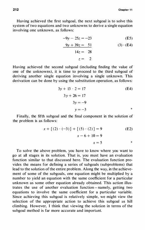
212 Chapter 1 1

Having achieved the first subgoal , the next subgoal is to solve this system of two equations and two unknowns to derive a single equation involving one unknown, as follows :

-9y - 25z = -23

9y + 39z = 5 1

1 4z = 28

z = 2

(E5)

(3 ) . (E4)

H aving achieved the second subgoal (including finding the value of one of the unknowns) , it is time to proceed to the third subgoal of deriving another single equation involving a single unknown. This derivation can be done by using the substitution operation, as follows:

3y + 13 . 2 = 1 7

3 y + 26 = 1 7

3y = -9

y = -3

(E4)

*

Finally, the fifth subgoal and the final component in the solution of the problem is as follows :

x + [ ( 2 ) . (-3 ) ] + [ ( 5 ) . ( 2 ) ] = 9

x - 6 + 1 0 = 9

x = 5

(E2)

*

To solve the above problem, you have to know where you want to go at all stages in its solution. That is , you must have an evaluation function similar to that discussed here. The evaluation function pro­vides the means for defining a series of subgoals ( subproblems) that lead to the solution of the entire problem. Along the way, in the achieve­ment of some of the subgoal s , one equation might be multiplied by a number to yield an equation with the same coefficient for a particular unknown as some other equation already obtained. This action i l lus­trates the use of another evaluation function - namely, getting two equations to involve the same coefficient for a particular variable. Since achieving this subgoal is relatively simple, we might view the selection of the appropriate action to achieve this subgoal as hi l l cl imbing. However, I think that viewing the solu tion in terms of the subgoal method is far more accurate and important.

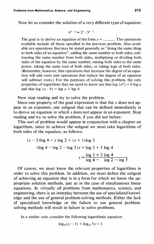
Probl em s from Mathematics, Science, and Engineering 213

N ow let us consider the solution of a very different type of equation :

The goal i s to derive an equation of the form x = __ . The operations available include all those specified in the previous problem. Also avail­able are operations that may be stated general l y as "doing the same thing to both sides of an equation" : adding the same number to both sides, sub­tracting the same number from both sides, mult iplying or div id ing both sides of the equation by the same number, rais ing both sides to the same power, taking the same root of both sides, or taking logs of both sides. (Remember, however, that operations that increase the degree of an equa­tion will add roots and operations that reduce the degree of an equation will subtract roots . ) For the purposes of solving this problem, the only properties of logarithms that we need to know are that log ( ab ) = b log a and that log ( a . b ) = log a + log b.

Now stop reading and try to solve the problem. Since one property of the goal expression is that the x does not ap­

pear in an exponent, one subgoal that can be defined immediately is to derive an equation in which x does not appear in an exponent. Stop reading and try to solve the problem, if you did not before .

This sort of problem would appear in conjunction with a chapter on logarithms, since to achieve the subgoal we must take logarithms of both sides of the equation , as fol lows:

(x - 3 ) log 4 = x log 2 + (x + I ) Iog 3

( log 4 - log 2 - log 3 )x = log 3 + 3 log 4

x = :--:lo-"g,-"3:-

+-,---,-3-;

I-,-,og,,,,--=-4_:---::­log 4 - log 2 - log 3

Of course, we must know the relevant properties of logarithms in order to solve this problem. In addition , we must define the subgoal of achieving an equation that is in a form for which we know the ap­propriate solution methods, just as in the case of simultaneous l inear equations. In virtual ly all problems from mathematics, science, and engineering, there is an interplay between the use of specialized knowl­edge and the use of general problem-solving methods . Either the lack of special ized knowledge or the fai lure to use general problem­solving methods will result in fai lure to solve problems.

I n a similar vein, consider the fol lowing logarithmic equat ion:

log l o (x - l ) + 10glO 5x = 1

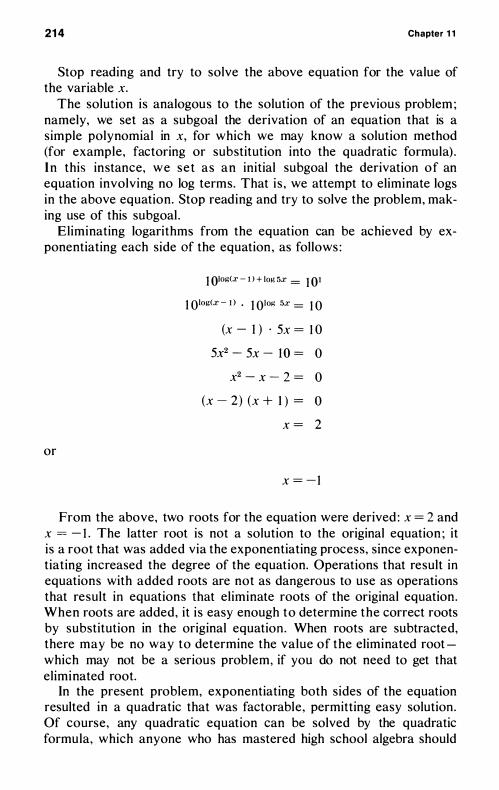
214 Chapter 1 1

Stop reading and try to solve the above equation for the value of the variable x.

The solution is analogous to the solution of the previous problem ; namely, we set as a subgoal the derivation of an equation that is a simple polynomial in x, for which we may know a solution method (for example, factoring or substitution into the quadratic formula) . In this instance, we set as an initial subgoal the derivation of an equation involving no log terms. That i s , we attempt to eliminate logs in the above equation. Stop reading and try to solve the problem, mak­ing use of this subgoal .

Eliminating logarithms from the equation can be achieved by ex­ponentiating each side of the equation , as follows :

or

1 010g(x - I ) + log 5x = 1 01

1 Olog(x - I ) • 1 Olog 5x = 1 0

(x - 1 ) . 5x = 1 0

5x2 - 5x - I O = 0

x2 - x - 2 = 0

(x - 2) (x + l ) = 0

x = 2

x = -1

From the above, two roots for the equation were derived : x = 2 and x = - 1 . The latter root is not a solution to the original equation ; it is a root that was added via the exponentiating process, since exponen­tiating increased the degree of the equation. Operations that result in equations with added roots are not as dangerous to use as operations that result in equations that eliminate roots of the original equation . When roots are added, it i s easy enough to determine the correct roots by substitution in the original equation . When roots are subtracted, there may be no way to determine the value of the eliminated root ­which may not be a serious problem, if you do not need to get that eliminated root.

In the present problem, exponentiating both sides of the equation resulted in a quadratic that was factorable , permitting easy solution . Of course, any quadratic equation can be solved by the quadratic formula, which anyone who has mastered high school algebra should

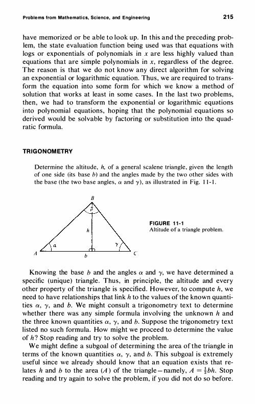
Problems from Mathematics, Science, and Engineering 215

have memorized or be able to look up. In this and the preceding prob­lem, the state evaluation function being used was that equations with logs or exponential s of polynomials in x are less highly valued than equations that are s imple polynomials in x, regardless of the degree. The reason is that we do not know any direct algorithm for solving an exponential or logarithmic equation. Thus , we are required to trans­form the equation into some form for which we know a method of solution that works at least in some cases . I n the last two problems, then , we had to transform the exponential or logarithmic equations into polynomial equations , hoping that the polynomial equations so derived wou ld be solvable by factoring or substitution into the quad­ratic formula.

TRIGONOMETRY

Determine the altitude, h, of a general scalene triangle , given the length of one side (its base b) and the angles made by the two other sides with the base (the two base angles, a and y) , as i l lustrated in Fig. 1 1 - 1 .

B

F I G U R E 1 1 - 1 Altitude o f a triangle problem.

A '-�---------u�----�� c b

Knowing the base b and the angles a and y, we have determined a specific (unique) triangle . Thus , in principle, the altitude and every other property of the triangle is specified . However, to compute h , we need to have relationships that l ink h to the values of the known quanti­ties a , y, and b. We might consu lt a trigonometry text to determine whether there was any simple formula involving the unknown h and the three known quantities a , y, and b. Suppose the trigonometry text l isted no such formula. How might we proceed to determine the value of h ? Stop reading and try to solve the problem.

We might define a subgoal of determining the area of the triangle in terms of the known quantities a , y, and b. This subgoal is extremely useful since we already should know that an equation exists that re­lates h and b to the area (A ) of the triangle - namely, A = l bh . Stop reading and try again to solve the problem, if you did not do so before .

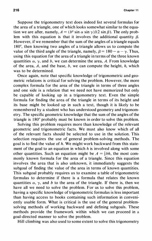
216 Chapter 1 1

Suppose the trigonometry text does indeed l ist several formulas for the area of a triangle, one of which looks somewhat similar to the equa­tion we are after, namely, A = ( b2 sin ex sin -y ) /(2 sin (3 ). The only prob­lem with this equation is that it involves the additional quantity {3. However, if we remember that the sum of the angles of a triangle equals 1 80°, then knowing two angles of a triangle allows us to compute the value of the third angle of the triangle, namely, {3 = 1 80 - ex - -y. Thus, using this equation for the area of a triangle in terms of the three known quantities ex , -y, and b, we can determine the area, A. From knowledge of the area, A , and the base, b, we can compute the height, h, which was to be determined.

Once again, note that specific knowledge of trigonometric and geo­metric relations is critical for solv ing the problem. However, the more complex formula for the area of the triangle in terms of three angles and one side i s a relation that we need not have memorized but only be capable of looking up in a trigonometry text. Even the simple formula for finding the area of the triangle in terms of its height and its base might be looked up in such a text, though it is l ikely to be remembered by a student who has understood geometry and trigonom­etry. The specific geometric knowledge that the sum of the angles of the triangle is 1 80° probably must be known in order to solve this problem.

Solving this problem requires more than knowledge of the relevant geometric and trigonometric facts. We must also know which of all of the relevant facts should be selected to use in the solution. This selection requires the use of general problem-solving methods. The goal i s to find the value of h . We might work backward from this state­ment of the goal to an equation in which h is involved along with some other quantit ies. Such an equation might be A = i bh , the most com­monly known formula for the area of a triangle . Since this equation involves the area that i s also unknown, it immediately suggests the subgoal of finding the value of the area in terms of known quantities. This subgoal probably requires us to examine a table of trigonometric formulas to determine if there is a formula that relates the known quantities ex , -y, and b to the area of the triangle. If there is, then we have all we need to solve the problem. For us to solve this problem, having a specific knowledge of trigonometric formulas i s less important than having access to books containing such information in conveni­ently usable form. What i s critical i s the use of the general problem­solv ing methods of working backward and defining subgoal s . These methods provide the framework within which we can proceed in a goal-directed manner to solve the problem.

H i l l c l imbing was also used to some extent to solve this trigonometry

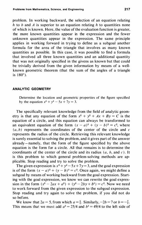
Problems from Mathematics, Science, and En gineerin g 217

problem. I n working backward , the selection of an equation relating h to h and A i s superior to an equation relating h to quantities none of which is known. H ere , the value of the evaluation function i s greater, the more known quantities appear in the expression and the fewer unknown quantities appear in the expression. The same principle appl ies in working forward in trying to define as a subgoal another formula for the area of the triangle that involves as many known quantities as possible. In this case, it was possible to find a formula that involved all three known quantities and an additional quantity that was not original l y specified in the givens as known but that could be trivial ly derived from the given information by means of a well­known geometric theorem (that the sum of the angles of a triangle i s 1 80° ) .

ANALYTIC GEOMETRY

Determine the location and geometric propert ies of the figure specified by the equation x2 + y2 - 5x + 7y = 3.

The specifical l y re levant knowledge from the field of analytic geom­etry is that any equation of the form x2 + y2 + Ax + By = C is the equation of a circ le , and this equation can always be transformed to an equivalent equation of the form (x - a ) 2 + (y - h ) 2 = ("2, where ( a , h ) represents the coordinates of the center of the circle and (" represents the radius of the circle . Retrieving this re levant knowledge is surely essential to solving the problem, and it gives part of the answer already - namely, that the form of the figure specified by the above equation is the form for a circ le . All that remains is to determine the coordinants of the center of the circle and its radius ( a , h, and c ) . I t is this problem to which general problem-solving methods are ap­pl icable. Stop reading and try to solve the problem.

The given expression is x2 + y2 - 5x + 7y = 3 , and the goal expression is of the form (x - a ) 2 + (y - h ) 2 = c2. Once again , we might define a subgoal by means of working backward from the goal expression. Start­ing with the goal expression, we know we can rewrite the goal expres­sion in the form (x2 - 2ax + a2 ) + (y2 - 2hy + h2 ) = ("2. Now we need to work forward from the given expression to the subgoal expression. Stop reading and try again to solve the problem, if you did not do so before.

We know that 2a = 5, from which a = � . Simi larly, -2h = 7 or h = -f . This means that we must add a2 = 25/4 and h2 = 49/4 to the left side of

218 Chapter 1 1

the given equation i n order to complete squares to get t o the left-hand side of the subgoal equation . The same 29/4 + 49/4 must, therefore , be added to the right side of the given equation, yielding 3 + 74/4, or 86/4. Thus , 86/4 = ('2 and (' = V86/2. Therefore , the coordinates of the center of the circle are ( i . -i ) , and the radius of the circle is V86/2, and the problem is solved .

Completing the square becomes a rather familiar specific technique in and of itself, once you have a certain degree of experience in mathematics . H owever, at some point to the beginning mathematics student, it is a new, unknown technique. To the same student, the technique of expanding a term of the form (x - a ) 2 to get (x2 - 2ax + a2 ) is famil iar. By using the general problem-solving method of working backward to get a subgoal , we can get the idea of completing the square in a completely natural way and know exactly how to do it.

Determine equations for the new coordinates of a point in a plane when the new coord inate system is obtained by translation and rotation from an old coordinate system. Translation of a coordinate system means the origin i s changed to a new point , and rotation of a coordinate system means both axes are turned through the same angle in the same direction, p ivoting about the origin .

I t makes no difference in which order the translation and rotation operations are performed ; the same new coordinate system is obtained in either case. Stop reading and try to solve the problem.

The solution of this problem results simply from breaking the prob­lem into parts, that i s , setting subgoals . First, solve the problem of characterizing the new coordinates obtained by simple translation alone. H aving achieved this subgoal , then solve the second subgoal of characterizing the final set of coordinates after a rotation has been applied to the coordinate system previously derived from the transla­tion. Stop reading and try to solve the problem again .

If x and y are the original coordinates , and the coordinates of the new origin in terms of the original (x, y) axes are (xo , Yo ) , then let the new coordinates obtained by translation be represented by XI , YI ' The formulas for simple translation of coordinates are as fol lows:

Y = Y I + Yo YI = Y - Yo

Stop reading and try to solve the rest of the problem, if you have not done so al ready.

Problems from Mathematics, Science, and Engineerin g 219

Let the coordinates obtained by rotation through the angle ex be X2 and Y2 . Formulas relating the new (X2 ' Y2 ) coordinates to the pre­vious (Xl ' Y l ) coordinates are as follows:

XI = X2 cos ex - Y2 sin ex

Yl = X2 sin ex + Y2 cos ex

To get formulas for the combined translation and rotation trans­formation, simply combine the above formulas to obtain the following :

X = X2 cos ex - Y2 sin ex + Xo

Y = X2 sin ex + Y2 cos ex + Yo

To express the new coordinates in terms of the old coordinates requires some algebra, from which yields the fol lowing:

X2 = X cos ex + Y sin ex - (xo cos ex + Yo sin ex ) Y2 = -x sin ex + Y cos ex - (-xo sin ex + Yo cos ex )

With the problem being broken into two subgoals , each of which was simpler to obtain , it was possible to obtain the solution to the original problem by simple algebraic combination of the solutions to the two subproblems.

Now let us consider the fol lowing problem involving the transforma­tion of coordinate systems :

I s it possible to transform axes such that the straight l ine 4x - 3y + 2 = 0 wi l l have the form XI = 0 and such that the straight l ine 2x + y = 4 wi l l have the form XI = aYI ? If such i s possible, derive the transformation.

Stop reading and try to solve the problem. Probably the first thing to note is that we have two equations and

two unknowns. If the equations are independent, which they are , then it will be possible to solve the equations for the value of X and y. From a geometric point of view, then, you must find the point of intersection of the two straight lines represented by these l inear equations. Solving for the point of intersection of the two straight l ines wil l prove to be an important subgoal in solving the problem, but you need not even real ize that in the beginning. Since solving these two l inear equations and two unknowns i s so simple, you should probably simply draw these

220 Chapter 1 1

inferences from the given information, without regard to the goal , at the outset of the problem (as discussed in Chapter 3 ) . This assumes, of course, that you are famil iar with the process of solving two l inear equations with two unknowns , so that this is a trivial inference. When it is easy to represent explicitly the information that is given implicitly in the problem, you should undoubtedly do so in the beginning, before even thinking about how to reach the goal from the given information. This initial step wil l y ield the information that the solution of the two equations (point of intersection of the two straight l ines) is x = I , Y = 2. Stop reading and try to solve the problem, if you did not before.

Consider the goal and derive a suitable plan for achieving the goal from the given information. H aving drawn the inference that the two straight l ines intersect at a particular known point, it is now clear that the goal is achievable. Why? Stop reading and try to solve the problem, if you sti l l have not done so.

The problem obviously indicates a division into two subproblems : (a) making the first l ine have the form Xl = 0 and (b) making the second line have the form Xl = aYI . Drawing inferences about these subgoals wil l point out the general types of transformation necessary to achieve each subgoal . Stop reading and try to solve the problem, if you did not do so.

It is somewhat easier to consider the achievement of the second subgoal first. The second subgoal equation, Xl = aYI , asserts that, in the new coordinate system, the second line will have zero Xl and Yl intercepts (being a strict proportionality) . Having zero XI and YI intercepts means that the equation of the second line must pass through the origin of the coordinate system. Having drawn this inference from the subgoal (or worked backward from the subgoal , if you wi l l ) , what transformation of the original coordinate system wil l achieve this new subgoal ? Stop reading and try to solve the problem, if you did not before.

Clearly, we can achieve the second subgoal by a simple translation of the coordinate system from the origin to any point on the second line (2x + Y = 4) . Our preceding inference concerning the point of intersection of the two straight lines might bias us to translate the origin of the coordinate system to the point of intersection of the two straight l ines, but at this stage of working on the problem we do not know for sure that this is the correct point of origin for the new coordinate system.

Now, how do we achieve the other subgoal , namely, that of trans­forming the first l ine so that it has the form XI = O? Stop reading and try to solve the problem, if you have not done so already.

Again drawing inferences from the subgoal (working backward), we

Problem s from Mathematics, Science, and Engineering 221

see that to transform the first l ine into a l ine with the equation XI = 0, we must transform the first l ine so that it is coincident with the Y axis in the new coordinate system. Such a l ine wil l always have the XI co­ordinate equal to zero for any value of the YI coordinate . Achieving this goal requires what type of transformation of the original coordinate system? Stop reading and try to complete the solution of the problem, if you have not done so already.

Clearly, to achieve this subgoal we must, first, translate the origin of the coordinate system to some point along the first line and , second , rotate the axis of the coordinate system to coincide with the first l ine . The first aspect interacts with the transformation necessary to achieve the other subgoal , so we are restricted to locating the origin of the new coordinate system at the point of intersection of the two straight l ines (since the origin of the new coordinate system must l ie on both straight lines). A second restriction in achieving the present subgoal is that the axis of the coordinate system must be rotated around this new origin until the Y axis coincides with the first straight l ine (4x - 3y + 2 = 0) . Geometric intuition indicates that this can be done and so achieving the goal is clearly possible .

Now the problem is to derive the nature of the rotation, since the translation is already obvious , that is, to move the origin to the point ( I , 2). To solve the rest of the prob lem, we now need to know the angle of rotation of the coordinate system required to line up the Y axis with the straight l ine represented by 4x - 3y + 2 = O. Stop reading and solve the rest of the problem, if you have not done so already.

To solve this subproblem let us write down the formulas for the new coordinates in terms of the old coordinates (noting that XI = X2 and YI = Y2 ) - namely, XI = X cos a + Y sin a - k, where k =Xo cos a + Yo sin a . We might also go ahead and write down the equation for YI i n terms of x, but this actual l y is unnecessary to the solution of the problem. I f we are continual ly aware of what terms represent constants and what terms represent variables in any expression, then we should note that, in the right side of the equation we have just written down, X and Y are the only variables , and cos a, sin a, and k are all constants (albeit unknown to us at present). Since given information specifies that XI = 0 and that 4x - 3y + 2 = 0, we can equate X cos a + y sin a - k to the expression 4x - 3y + 2.

Now if we take the equations for the general transformation of coordinates involving both translation and rotation and substitute them into the equation 4x - 3y + 2 = 0 we obtain

4 (xl cos a - YI sin a + xo ) - 3 (xl sin a + YI cos a + Yo ) + 2 = O.

222 Chapter 1 1

Since w e wish t o find a n a for which X l = 0 , w e can substitute X l = 0 into the above equation and also substitute the known values of Xo = 1 and Yo = 2. This yields the equation

- (4 sin a + 3 cos a )YI = 0

This equation implies that 4 sin a + 3 cos a = O. Thus , 4 sin a = -3 cos a. To determine a from this equation, simply remember the trigo­nometric identity that sin a/cos a = tan a. We can then derive from the above that tan a = -� = -0.75 . U sing the tables, this indicates that a = -3 6° 5 2 ' . Thus , the solution to the problem is to translate the origin of the coordinate system to the point ( 1 , 2) and rotate the co­ordinate system through an angle of 3 6° 52 ' in the negative direction.

One sl ightly tricky aspect of the problem is the use of the equation X l = 0 in conjunction with the equation derived by substituting into 4x - 3y + 2 = O. After we have establ i shed that it is indeed possible to derive a transformation of the coordinates so that the equation 4x - 3y + 2 = 0 can be transformed into an equation of the form X l = 0, we are not real ly trying to achieve the goal expression X l = O. Rather Xl = 0 i s part of the given information that we are using to achieve the subgoal of determining the angle of rotation a. This problem clearly points up the need to careful ly define and redefine what is given information and what i s the goal at different stages in the solution of the problem.

CALCULUS

Prove that , within the set of triangles having a constant base and constant perimeter, the isosceles triangle has the maximum area.

The specific calculus necessary to solve this problem is to know that we can often find the maximum or minimum of a function by differ­entiating it with respect to the variable(s) of which it is a function. Stop reading and try to solve the problem.

Clearly, in the present instance, the function (dependent variable) is the area of a triangle. However, the area of a triangle can be expressed as a function of a number of different independent variables. Therefore , let us set the subgoal of finding a formula for the area of a triangle that involves those quantities that are specifical ly given in this problem (either constants or the variables with respect to which we wish to find maximum area). Stop reading and try again to solve the problem, if you did not do so before .

In thi s problem, the constants and independent variables are evi­dently the sides of the triangle ( including the sum of the sides, which

Problem s from Mathematics. Science. and Engineerin g 223

i s the perimeter) . Thus , we need to find a formula that involves only these quantities. Such a formula, which can be looked up in a book, i s Heron' s Formula: A = [s ( s - a ) ( s - b) ( s - c) ] 1 12, where A is the area of a triangle ; s i s the semi perimeter, which equals l ( a + b + c ) ; and a, b, and c are the lengths of the sides. Stop reading and try to solve the problem, if you have not done so already.

Having achieved the first subgoal of finding a formula that involves the relevant constants and variables, we should note that the formula contains the semiperimeter (which is a constant, since the perimeter i s a constant) and the length of one side (which is a constant ; let i t be side a). Two variable sides remain - namely, b and c - and we might achieve the solution by simply differentiating A with respect to both b and c. However, suppose we are famil iar only with differentiating functions of single variables with respect to the single variable in order to obtain the maximum or minimum of the function with respect to that variable . I n this case, we must set a second subgoal to reduce the number of independent variables from two to one. Stop reading and try to solve the problem, if you have not already done so.

We can achieve the second subgoal , since with a constant perimeter and a constant base (a ) , the sum of the other two sides must be equal to a constant. Thus , b + c = k and c = k - b. Substituting c = k - b into Heron's Formula for the area of a triangle, we obtain the area as a function of a single variable, namely, the length of side b. This can be differentiated with respect to b and the derivative set equal to zero to determine that k = 2b. A trick that makes this a bit easier i s to note that, i f the area A i s a maximum, then A 2 i s a maximum and vice-versa. Since it is somewhat easier to differentiate A2 with respect to b than to d ifferentiate A with respect to b, th is l i ttle trick saves some work. In either case, we solve for k = 2b, from which it fol lows that b = c, and the theorem is proved . The work is given below :

A 2 = s ( s - a ) ( s - b ) ( s - c )

A 2 = s (s - a ) ( s - b ) ( s - k + b )

dA 2/ db = s ( s - a ) [ (-1 ) ( s - k + b ) + ( s - b ) ( + 1 ) ] = 0

-s + k - b + s - b = 0

k - 2b = 0

k = 2b

b + c = 2b

c = b

224 Chapter 1 1

I nc idental ly, the above problem can b e solved entire ly without cal­culus , us ing the method of contradiction in conjunction with Heron's Formula. To use the method of contradiction, we assume that the squared area (An in the case where b2 =l= C2 is greater than the squared area (An in the case where b l = C I = d. Without loss of generality, assume b2 > C2 . Since b2 + C2 = 2d, then b2 > d > C2 ' U sing these equal i­ties and inequalities and some algebraic manipulation of the equation (s - b2 ) ( s - (2 ) > (s - d) 2, we can eventual ly derive ( b2 - c2/ 2) 2 < 0, which is a contradiction since the square of any real number must be positive. The algebra i s given below for the interested reader:

Derive the form of the fol lowing indefinite integral :

y = f I +IXIl2 dx

The background i nformation that is assumed to be given includes knowl­edge of the i ntegrals of elementary functions (such as xn, eX , log x, s in x, and cos x). Other important background information are the techniques of integration by substitution and by parts , and differentiating a function of a function.

The first major choice in attacking an integration problem of this kind is whether to use the method of substitution or the method of integration by parts. Sometimes both methods must be used , but, in any event, you stil l have to decide which to apply first. Since integra-

Problems from Mathematics, Science, and Engineerin g 225

tion by substitution is the more useful technique, it is to be preferred as an initial choice of integration method , unless there is some special reason for preferring integration by parts. I ntegration by parts is usefu l primari l y when the function to be integrated is a product of two func­tions [f(x) = g(x)h (x) ] . Although al l functions of x can be written as a product of two functions - namely, f(x) = f(x) . I - this i s a trivial type of product to which the application of integration by parts is only occasional ly usefu l . Thus , in the present problem, there is no reason to use integration by parts, so we adopt integration by substi­tution as our initial operation. Stop reading and try to solve the problem.

Note that the problem-solving method considerations discussed so far in this problem are all specific to calcu lus . Substitution and inte­gration by parts are not general problem-solving methods. H owever, in deciding what type of substitution to make, general problem-solving methods play some role . In particular, hil l c l imbing i s usefu l . The hi l l climbing u ses an evaluation function concerned roughly with simplicity of functional form and the l ikel ihood of your knowing an integral for the function resulting from this substitution. At the same time , another evaluation function i s general ly working at cross purposes with the first one - namely, the simplicity of the functional form for the substi­tution u = g (x) . A good rule of thumb is to try a substitution whose functional form is less complicated than that of the original function and results in a function to be integrated that i s also less complicated than the original function. Thus , in the present problem, although a substitution of the form u = ( 1 + XI /2 ) - 1 would greatly simpl ify the original problem, the form of the substitution function would be as complicated as the original function to be integrated . Stop reading and try again to solve the problem, if you did not before .

Better substitutions would be u = Xl /2 or u = 1 + xl l2 . U sing the latter substitution, u = 1 + Xl /2 and dx = 2 ( u - 1 ) du, yields

J 1 +Ix1/2 dx = 2 J (u � 1 ) du = 2 J 1 - � du = 2 ( u - log u ) + c

= 2 ( 1 + X1/2 ) - 2 log ( 1 + x1 l2 ) + C

= 2x1 l2 - 2 log ( 1 + x1 l2 ) + K

Frequently, several substitutions wi l l be required in order to solve the problem, and , at each step you are essential ly us ing the method of hi l l cl imbing on an evaluation function concerned with simplicity of functional form. There is no precise definition of simplicity of func­tional form, but that lack sho!.I1d not prevent you from explicit ly recog­nizing that this is what you are doing and that you have rather good

226 Chapter 1 1

judgment a s t o what functions are simpler than other functions ( in the sense of being closer to functions for which you know the integral) . As long as you are able to decide that the functions resulting from certain substitutions are simpler than functions resul ting from other substitutions, you are in a position to make good use of the hil l­c l imbing method , whether or not you can explicitly define the evalua­tion function.

Derive the functional form of the fol lowing integral : f x2 eX dx. The spe­cific background knowledge includes knowledge of the integrals of the elementary functions plus the integration by parts formula - namely, f uv dx = u V - f u ' V dx, where V = f v dx and /I ' = du/dx .

Since the function to be integrated is an obvious product of two simpler functions, the method of integration by parts is suggested. Whether integration by parts i s making progress toward the goal is determined a great deal by the general problem-solving method of hi l l c l imbing on an evaluation function of simplicity of functional form and ease of integration. Stop reading and try to solve the problem.

In the present case, two applications of the method of integration by parts is necessary in order to solve the problem. At each stage the appl ication of integration by parts results in functions to be inte­grated that are simpler than the functions to be integrated prior to the application of integration by parts. The specific solution is as fol lows:

J x2eX dx = x2ex - J 2xex dx + K = x2ex - 2xe.r + 2e.l' + C

= (x2 - 2x + 2 ) eX + C

I n the present instance, it would be possible to give a precise defini­tion of the evaluation function on which the hill c l imbing is occurring ­namely, the exponent of x in the product x"eX when this product is the function to be integrated. Repeated application of the method of integration by parts results in reduction of the exponent, eventual ly to xOex or eX . However, whether or not it is possible to explicitly define the evaluation function being used , h i l l -c l imbing methods can be ex­tremely u seful in solving such a problem, so long as your judgment of simplicity i s reasonably accu rate.

Find the values of x for which the function y = f(x) i s a maximum or minimum. The function i s defined by the equation r + xy + y2 = 27. Rele­vant background information includes the chain rule for differentiat ing the function of a function, the ru le for differentiating the product of two functions, and the theorem that the derivative of a function equals zero at a minimum or maximum.

Problems from Mathematics, Science, and Engineerin g 227

When we are finding the maxima or minima of even a function of a single variable, y = f(x) , we are essential ly solving two equations for the values of two unknowns, x and y. This fact is often not apparent to students when they original ly learn the method of finding maxima and minima by differentiating f(x) , setting it equal to zero, and solving for x, because the original equation was already solved for y as a function of x. I n such a case , the derivative wil l involve only a single variable x. When the derivative is set equal to zero, the resulting equation is solved for the value of x for which the function is a maxi­mum or minimum. I n the present problem, the initial function y = f(x) i s defined implicitly by the equation .xl! + xy + y2 = 27. In this case, it is necessary to take a more general approach to the problem, in which finding the derivative and setting it equal to zero al lows us to obtain a second equation, in addition to the equation x2 + xy + y2 = 27 . We hope that these two equations wil l permit us to solve for the (x, y) points for which the function has a maximum or minimum. Stop reading and try to solve the problem.

To solve the problem, we should initial ly set a subgoal : to obtain an equation that involves the derivative y' = dy/dx. Stop reading and try again to solve the problem, if you did not before .

This subgoal can be achieved by differentiating the given equation with respect to x (employing the product and chain rules for differenti­ation). The resulting equation is 2x + xy ' + y + 2yy ' = o. This equation can be solved for y' by algebraic manipulation, yield ing the equation

, _ -(2x + y ) y - x + 2y

When this equation is set equal to zero , we obtain y = -2x. Substi­tuting this equation into the original equation, we obtain x2 - 2x2 + 4x2 = 27 or 3x2 = 27 or x = ±3 , Y = ±6, and the problem is solved . Once again, a simple definition of a single subgoal - namely, obtaining an expression for y ' in terms of x and y - resulted in straightforward solution of the problem.

DIFFERENTIAL EQUATIONS

The solutions of differential equations provide particularly good ex­amples of the use of the problem-solving methods of hi l l c l imbing, subgoals , and analogy to similar problems. Perhaps the most important specific training is the ability to place a differential equation in the proper class. Once you note what other differential equations the one in front of you is similar to (what c lass it belongs to), you can then

228 Chapter 1 1

apply the techniques associated with the solution of that class of dif­ferential equations . You need not even have much specific knowledge of how to solve equations of a particular class, so long as you can identify the class and look up in a book how to solve equations of that class . Thus , analogy to similar problems is the crucial first step in the solution of many differential equations .

When the given differential equation is a member of a c lass for which solution methods are known, the methods of hill cl imbing and sub­goals (using evaluation functions) are also quite important. For ex­ample, in solving differential equations of different forms, we often proceed by setting as a subgoal the transformation of the differential equation into another differential equation of simpler form, and then by using the known solution methods for the simpler form.

In grab-bag classes of differential equations (such as miscellaneous nonlinear differential equations) , we may attempt to define subgoals such as transforming the equation to l inear form or reducing the order or degree of the equation, but frequently we simply try out various operations on the given nonlinear differential equations to see which ones result in an equation of the s implest form. The latter is clearly an example of hi l l c l imbing, using an evaluation function that somehow weights different features of a differential equation for overall ease of solution.

For equations with order m and degree n (m , n > 1 ) , the relevant evaluation function is frequently the vector (m , n ) , with lower values of either m or n being more highly valued . Differential equations pro­vide good examples of vector evaluation functions , where there are many different properties on which hi l l c l imbing might be tried to see which, if any, approach would solve the problem. Frequently, the solution of a differential equation requires a sequence of steps in which the degree and order of the equation are progressively reduced , final ly resulting in a differential equation of the first order and first degree. The order in which the degree and order of the differential equation is progressively reduced may vary from problem to problem.

Once the stage is reached where you have a nonl inear differential equation of the first order and first degree to solve, a variety of poten­tial solution sequences can fol low, again depending on the type of first-order, first-degree differential equation .

The nonlinear differential equation may be reducible to linear form by some su itable transformation . No general rules exist for determining such transformations nor the types of nonlinear equations to which they apply, but experience with a wide variety of such problems may indicate that the present problem is similar to some problem already

Problems from Mathematics, Science, and Engineering 229

solved in this way. H aving achieved a l inear equation of the first order and first degree, you then apply solution methods appropriate to this type of equation (for example, us ing Laplace transforms or inte­grating factors) .

Another solution sequence starting with a nonlinear, first-order, first-degree differential equation (which is appropriate in some cases) i s to try to transform the equation to be a member of a particular class of d ifferential equations known as exact differential equations. Achiev­ing thi s subgoal may require you to find an appropriate integrating factor to transform the given d ifferential equation into an exact dif­ferential equation. Once an exact differential equation has been ob­tained , you simply fol low solution methods appropriate for this type of equation.

Another solution sequence is appropriate to d ifferential equations of the form

dy a 1x + b1y + CI dx = a2X + b2y + C2

where a 1b2 - a2b l ¥- O. To solve such equations, we set the subgoal of transforming this inhomogeneous equation into a homogeneous equa­tion by making a substitution. The next subgoal i s to transform this homogeneous equation into a d ifferential equation in which the variables are separated , which is then solved by direct integration.

There are other solution sequences appropriate to other types of nonlinear differential equations of the first order and first degree. However, just considering the solution sequences discussed here , note that an experienced solver of differential equations has estab­l ished an evaluation function for first-order, first-degree differential equations , which i s essential ly a partial ordering of a variety of dif­ferent forms of such differential equations. I n this partial ordering, equations with separated variables are more highly valued than homo­geneous equations in which the variables are not separated , the latter being more highly valued than the type of inhomogeneous equations described above, which in turn are more highly valued than many nonlinear differential equations not of this or any other identifiable type. At the same time, exact differential equations are more highly valued than these miscel laneous nonlinear d ifferential equations, but there i s no relative ordering of exact d ifferential equations relative to equations within another solution sequence , such as that appropri­ate for the inhomogeneous equations of the previously specified type. Along the same lines, l inear d ifferential equations are more highly

230 Chapter 1 1

valued than the miscellaneous nonlinear differential equations, but they are not necessarily more highly valued than types of equations within some other solution sequence. This is what we mean by saying that these different types of first-order, first-degree differential equa­tions have an evaluation function in the form of a partial ordering, rather than in a complete or simple rank ordering of all the different types of such equations.

I f we know a variety of such types of differential equations and the appropriate partial ordering type of evaluation function defined over them (that is, know the variety of different solution sequences), we are in a good position either to define subgoals or to recognize progress in the use of the hil l-cl imbing method . However, there is stil l the prob­lem of determining the proper operation (substitution, integrating fac­tor, and the l ike) to take in order to achieve a differential equation of the more highly evaluated (simpler) form. Perhaps general problem­solv ing methods are applicable to this aspect of solving differential equations, but, frankly, I have so little experience in solving differen­tial equations that I feel incompetent to discuss the matter further.

I n any event, once again, a solution of mathematical problems re­quires a mixture of specific knowledge of mathematics and the use of general problem-solving methods . You can, of course, learn how to solve differential equations and other mathematical problems without apprec iating that you are thereby apply ing general problem-solving methods . H owever, understanding general problem-solving methods probably facil itates your understanding the variety of techniques appl icable to such mathematical problems. A general ly accepted dogma in educational psychology is that the more you can relate new knowl­edge to old knowledge , the faster and more complete your learning will be (though how good the evidence for this is I certainly do not know). So, if you know general problem-solving methods you should be able to quickly organize many specific methods for solving differ­ential equations when these methods are introduced in terms of de­fining classes of similar problems and defining evaluation functions that permit you to use the subgoal and hil l-cl imbing methods .

To complement th is rather abstract discussion, let us consider the solution of the fol lowing differential equation , which was produced by AI Stevens, a student in one of my problem-solving classes :

2y2 ---.l!. + 2y ...1 = 1 d2 ( d ) 2 dx2 dx

Stop reading and try to solve this differential equation.

Problems from Mathematics, Science, and Engineering 231

Stevens first defined as a subgoal the transformation of this equa­tion into a l inear, second-order differential equation, but he quickly re­placed this subgoal with a different subgoal - namely, that of reducing the equation from second order, nonlinear to first order, nonlinear. Stop reading and try again to solve the problem, if you did not do so before .

The second subgoal is easi ly achieved because the differenl!ial equa­tion is of the form cPy/dx2 = f(y , dy/dx) , with cPy/dx2 not being a function of x. By recognizing the differential equation as a member of this class, Stevens made avai lable his knowledge that a standard substitution - namely, v = dy/dx- would transform the second-order differential equation into a first-order differential equation.

Since dv/dx = d2y/dx2 and dv/dx = (dv/dy ) (dy/dx) , then cPy/dx2 = v dv/dy. Substituting into the original equation yields the first-order nonl inear differential equation 2y2v dv/dy + 2yv2 = 1 . Stop reading and try again to solve the problem, if you d id not do so before.

Algebraic manipulation of the equation yields dv/dy + y- I V = ly-2V- I . Such an equation belongs to another specific class of differential equa­tions - namely, Bernoul l i equations - which are of the form

dv dy + P (y ) v = Q (y ) vR

You can look up in a book that such equations can be reduced to l inearity by the substitution w = vl-n. I n this case , that means the substitution w = v2, for which

v = wl/2

Substitution then yields

and dv _ 1 W- 1 /2 dw dy - 2 dy

dw 1W- 1 /2 - ..L y- I w1 /2 - 1y-2W- 1 /2 2 dy I - 2

Multiplying through by 2Wl /2 yields

dw - + 2y- I w = y-2 dy

which is a l inear equation in w and y. From this point, the solution i s straightforward by methods that can be looked up in a book.

I n retrospect, Stevens noticed that his first-order, nonlinear differ­ential equation, 2y2v dv/dy + 2yv2 = 1 , had the form d (y21 '2 ) /dy = 1 ,

232 Chapter 1 1

in which the variables y and y2v2 are trivially separable. Thus , the equation is easi ly solvable without it having to be reduced to l inear form. The solution is as follows :

I ntegrating,

Since v = dyjdx,

y2 (iY = y + c1

y i = (y + Cd l /2

J (y +yc1 ) 112 dy = J dx

From a table of integrals ,

-2 (2c1 - y ) ( C I + y ) l /2 = X + C2 3

PROBABILITY AND STATISTICS

A sample of two observations , x and y, are drawn from the uniform dis­tribution on the interval from zero to I , f(x) = f(y) = I , 0 "" x, y "" I . Find the rth raw moment of z, (ILr : . ) , where z = xy. Note that

ILr: . = foo zrg ( z ) dz

There are at least three different ways of solving this problem. Stop reading and try to think of as many ways as you can.

The most obvious (but also the most difficult) way i s to set two subgoal s : (a) that of finding the probabil ity density function [ g(z) ] for the new random variable z = x . y and (b) that of plugging this proba­bil ity density function into the definition for the rth raw moment of z.

Let us assume that we know a simple generalization of the above formula that extends it in order to find the rth moment of a junction of random variables, h (x, y ) , where the joint probabil ity density func-

Problems from Mathematics, Science, and Engineerin g 233

tion for the random variables x and y is represented by f(x, y ) . The formula i s

f.Lr: h(x. y ) = L"oo [h (x, y ) Y f(x, y ) dxdy

Now stop reading and try to solve the problem, if you did not do so before .

I n this case, we can compute the rth moment of the function z = x . y, provided we know the probabil ity density function of the joint distribu­tion of x and y. Thus, the first subgoal is to determine this function, f(x, y ) . We must assume as implicit information (though it was not specifical ly stated in the problem) that the two sample observations (x and y) are independent or uncorrelated . Knowing these observations are independent and knowing the density functions for each, we get the joint density function f(x, y ) = f(x)f(y ) = I , 0 S x, y s I , f(x, y ) = 0, el sewhere. From this point on, the solution is a simple integra­tion , as follows :

f.L,. : z = f.Lr: h(x. y) = l' (x yV f(x, y ) dxdy

= l' xr dx . l' yr dy ( r + 1 ) 2

Final l y, one can set a totally different subgoal of finding the moment generating function for the new variable z = xy and differentiating the moment generating function r times to find the rth moment of z. I n solving the problem b y this method, w e need to know more specific background information (such as the definition of a moment generat­ing function and the Taylor series expansion for e 8x) , but otherwise the problem is solved in a straightforward manner by this method as wel l .

The principal general problem-solving method used to solve this problem was the setting of subgoals . A variety of such subgoal s were logical ly related to the solution of the problem - namely, that of de­riving the probabi l ity density function g (z ) , that of deriving the joint distribution function f(x, y ) , or that of deriving the moment generating function for z. Setting the subgoal s in each case i s a part of an overal l calculative plan for solving the problem in each of the three cases . For example, a first step in solving the problem might be to write down

234 Chapter 1 1

the formula for the rth moment of z in terms of a double integral of (xyV and the joint probabil ity density function f(x, y ) . This would suggest that we needed to determine the joint probabi l i ty density func­tion as a subgoal in order to do the integration and solve the problem.

The lengths of two parts , A and B, are normal ly distributed with means 11-04 = 2 centimeters and I1-H = 4 centimeters and standard deviations <TA = 0.03 centimeter and <Til = 0.04 centimeter. One A piece and one B piece are randomly assembled and laid end to end to form a length about 6 centimeters long. If the assembly is to fit certain qual i ty control stan­dards , it must be between 5 .9 1 and 6 .09 centimeters long. What per­centage of such assemblies wi l l fai l to fal l within these l imits?

Stop reading and try to solve the problem. We set as a subgoal that we must determine the distribution function

for the sum of two random variables, A and B. We know from back­ground stati stical knowledge that , if A and B are normally di stributed random variables, then A + B will be a normal ly di stributed random variable with a mean equal to the sum of the means of the component random variables and a variance equal to the sum of the variances. Thus , /J-A + B = 6 centimeters and O"A + B = \1'0.032 + 0.042 = \1'0.052

= 0.05 . H aving achieved the subgoal of determining the distribution function for the random variable A + B, we now set the second and final subgoal to be to determine what percentage of the distribution lies outside a region of 0.09 on either side of the mean. This subgoal can be determined from a table of the normal distribution, provided we know how many standard deviations is represented by 0.09 centi­meter. To determine this amount we simply divide 0.09 by 0.05 to get 1 . 8 standard deviation units, tel l ing us that we are asking for the per­centage of cases fall ing in the two tai ls of a normal distribution 1 . 8 standard deviation units out from the mean. Looking up the value z = 1 . 8 in a table of the normal d istribution gives the figure of 0.036 in one tail or 7.2 percent in both tai l s . Once again, the solution of the problem proceeds from our setting a series of one or more subgoals that, taken together, constitute the solution to the entire problem.

Determine one way in which the random variable z might have been formed , where the moment generating function of z i s

e4B + ( 8'12 ) Mz«(}) = ( 1 _ 2(})312

Stop read ing and try to solve the problem.

Problems from Mathematics, Science, and Engineering 235

I n contrast to earl ier problems, in this one the goal is specified but the givens are not, and we must determine some set of givens such that the goal - namely, the moment generating function - can be de­rived as a consequence. The obvious way to check out any hypothe­sized set of givens is to use the method of contradiction. I n addition, we should use the method of working backward from the goal expres­sion, since th is is a unique starting point in the problem. The most relevant piece of background information is that the moment generat­ing function of a sum of random variables is the product of the moment generating functions of each component random variable. Stop read­ing and try again to solve the problem, if you did not before .

By examining a table of such moment generating functions, we can quickly exclude the possibil ity that the moment generating function of z is itself a random variable with a simple standard di stribution function .

The next simplest hypothesis would be that z is the sum of two ran­dom variables, each of which has a simple famil iar di stribution func­tion . This being the case, we should work backward from the goal expression by factoring it into two components, each of which is a moment generating function for a famil iar distribution function. The most obvious split of the goal moment generating function i s probably to multiply the numerator times the reciprocal of the denominator. I t turns out that the numerator is the moment generating function for a normal distribution with mean 4 and standard deviation I , and the rec iprocal of the denominator is the moment generating function for a random variable of the X 2 distribution on 3 degrees of freedom, which means that z i s the sum of these two random variables .

Had this particu lar factorization not worked , there are a number of other simple factorizations of the moment generating function that might have been matched for form against our table of moment generat­ing functions for famil iar distributions. I n many ways , the solution of the problem is terribly simple . We can ask, " H ow can we not start with the goal expression, which is the only given in the problem other than implicit given information?" I ndeed , if we start to manipulate the goal . expression and know the relevant background information about the moment generating functions, it i s difficult to sec how we can fai l to solve the problem. Nevertheless , many people do fai l to solve this problem and other equal l y simple problems, because they have no idea what to do. In many cases, they are genuinely deficient in important background information, but those who knew they had to work backward from the goal expression in the present problem wou ld l i kely look up in books the relevant information about moment

236 Chapter 1 1

generating functions that was needed in order to solve the problem. Those who have a thorough knowledge of the specific subject matter probably need to have no conscious understanding of general problem­solving methods in order to solve this and many other problems. H owever, those who are learning the specific subject matter will be aided in this learning by a thorough knowledge of general problem­solving methods , which suggest what types of information are needed in order to solve problems.

Again , in the problem with the two pieces A and B that are joined end-to-end to form a new combined piece that must fall within certain tolerance l imits, students might lack the specific background informa­tion about the d istribution function of the sum of two normal ly dis­tributed random variables. H owever, having clearly defined the subgoal of determining such a di stribution function in order to determine the percentage of cases that l ie in its tai l s , it is l ikely that students would look for the directly re levant piece of information they lacked .

Formulas for getting certain information from other information often automatically provide you with a set of subgoals - namely, that of determining the values of the various components of these formulas. Thu s, if you have enough specific background information to know the appropriate general formulas, you can often substitute that informa­tion for an understanding of general problem-solving methods in those cases where you know some general formula that encompasses all the aspects of the problem. H owever, if no such formula exists or if you do not know it, understanding general problem-solving techniques can be qu ite crucial in devising an adequate plan to solve the problem.

COMBINATORIAL ANALYSIS

How many ways can a set of contestants consist ing of four men, three women, two boys, and three girls be selected from an audience consist ing of eight men, nine women, six boys, and s ix girl s?

Stop reading and try to solve the problem. To solve the problem, we might set a series of subgoal s ; that i s , we

might determine how many ways there are to pick first the men alone, then the women alone, then the boys alone , and then the girl s alone. Let us call the solutions to these four subproblems N ] o N2 , Na , and N4 • Stop reading and try again to solve the problem, if you did not before.

The number of ways to pick an entire set of contestants is simply the product N 1 • N 2 • N:! . N 4 ' Each of the subgoal s is a simple combina-

Problems from Mathematics, Science, and Engineering 237

tions problem (unordered sets obtained by sampling without replace­ment) . Thus , the total number of ways is simply

( 8 . 7 . 6 . 5 ) ( 9 . 8 . 7 ) (�) ( 6 . 5 . 4 ) 1 · 2 · 3 · 4 1 · 2 · 3 1 · 2 1 · 2 · 3

John and Fred agree to play a tennis match , with the winner to be the person who first wins two sets in a row or a total of three sets. Find the number of ways the match can occur.

Stop reading and try to solve the problem. The most straightforward way to determine the number of ways the

match can occur is to construct a tree diagram, marking all terminals of the tree where either one of the conditions i s first satisfied and stop­ping the growth of the tree from that point on. The tree has two branches at each node - namely, A wins or B wins .

Alternatively, we can determine the answer without expl ic i t ly con­structing the tree, by the fol lowing line of reasoning. We first make certain inferences from the information given in the problem - namely, that the match cannot end before two sets have been played and must end after a max imum of five sets have been played (s ince out of five sets one player must win at least three sets) . H aving made these in­ferences, the problem of determining the number of ways the match can occur can be reduced to a set of four subproblems - namely, we must determine how many ways the match can end after two sets, three

sets, fou r sets, or five sets. Stop reading and try again to solve the prob­lem, if you did not before .

Clearl y, there are on ly two ways the match can end after two sets ­namely, A wins both sets or B wins both sets. There are also only two ways the match can end after three sets : A wins the first set and B wins the next two, or B wins the first set and A wins the next two. Now we might note that , in general , at each level of the tree, after the second , there wil l be exactly two terminal nodes and two nonterminal nodes u nder the ru le that the winning p layer must win two sets in a row. Thus , at every node prior to the last, there wi l l be e xactly two terminal nodes and two nonterminal nodes . At the last node , there wi l l be four terminal nodes , since, by the three-set rule , al l nodes mu st be terminal once five sets have been played. Thus , there are two terminal nodes after two sets, two terminal nodes after three sets , two terminal nodes after four sets , and four terminal nodes after five sets, or 1 0 termi nal nodes in all (and so 1 0 ways the match can occur).

238 Chapter 1 1

The principal general problem-solving methods used in solving the problem were inference and the subgoal method . N ote that although the spec ial ized method of expl ictIy constructing a tree diagram wi l l a lso solve this problem without the need for using the more general subgoal method , the subgoal method in combination with certain in­ferences general izes easi ly to problems in which to construct an ex­p l ic it tree would be extremely laborious.

John pays a quarter to play a simple coin-flipping game against a gambling casino. The quarter entitles h im to play a maximum of five coin flips against the house. John wins $ 1 every t ime he cal l s the coin correct ly (head or tai ls) and loses $ 1 every t ime he cal l s the coin incorrectly . John begins with $3 and wil l stop playing whenever he loses h is ent ire stake or wins $3 (that i s , has a total of $6) . Of course, he must quit after playing a maximum of five coin flips . Find the number of ways the .play­ing can occur.

Stop reading and try to solve the problem.

A first general problem-solving method we might use is to note the similarity to the previou s problem. This s imi larity leads to the conjec­ture that we could solve the problem either by constructing an explicit tree diagram or by making certain inferences about the tree diagram and then breaki ng up the problem into subproblems to determine how many ways the playing can occur, stopping after N coin flips, for all N :-s 5 . Stop reading and try again to sol ve the problem, if you did not before .

One simple inference is that John must play for at least three coin flips, since, at worst, he will loose $ 1 on each coin flip, and he has $3 to play with . S ince he can play at most for five coin flips for his original quarter, we know that we can break the problem into three sub­problems - namel y, to determine how many ways the playing wi l l stop after three , four, and five coin flips . C learly, there are exactly two ways the p laying wi l l stop after three coin flips (two terminal nodes) , leav­ing s ix nonterminal nodes after three coin flips. Another relevant in­ference is that it is impossible to be ahead or behind by an even number of dol lars after any odd number of coin flips (such as three flips) . Thus , it i s impossible for John to be either even or ahead or behind by $2 after three flips . H ence, the s ix nonterminal nodes must all in­volve d ifferent sequences of winnings and losings that total either

+$ 1 or -$ 1 , and , by symmetry, there must be three of each type. From this we can conclude that there are no terminal nodes after four coin flips and 1 2 nonterminal nodes. The 1 2 nonterminal nodes at level

Problems from Mathematics, Science, and Engineering 239

4 lead to 24 nodes at level 5 , all of which, by definition, must be ter­minal . Thus , there are precisely 26 different ways the playing can occur.

Binomial theorem. Prove that

( a + b ) /1 = � n_ ( n) all - r • br Lor - o r

( n) n ! where =

' ( _ ) ' r r . n r .

The basic problem-solving method to be used i s mathematical in­duction, which we have already noted involves a combination of the general problem-solving methods of special case ( proving the theorem true for n = I) and the subgoal method (dividing the proof of the theorem into two parts : proving it true for n = 1 and showing that , if it is true for n , the theorem is true for n + I ) .

Stop reading and try to solve the problem. The theorem is trivial ly true for n = I , so the crux of the proof con­

sists of assuming that the theorem holds for (a + b ) n and proving it is true for (a + b ) " + l . To prove this lemma, we assume the theorem is true for n and multiply both s ides of the equation by ( a + b ) . This operation yields the term ( a + b) n + 1 on the left side of the equation , a s desired . The right side o f the equation wi l l c learly i nvolve exactly

n + 2 terms of the form an - r • br, where r goes from zero to n + I , as desired. This is obvious by inspection. What remains i s to prove that

the coefficients of each a " - rbr term have the form (n � I ) . Except for

the terms a n + l and bn + l , which ari se only once in the multiplication of

( a + b ) L;= o ( ;)an - rbr, every other an - r . br term arises in two places .

The term i n the product that contains b r i s obtained from

b[ C� I )all - r+ l br- l ] + a [ (;)an - rbr] = C� l )all - r+ Ibr + (;)all - r+ Ibr = [C� I ) + (;) ]an- r+ 1br

Al l that remains is to show that [C� I ) + e)] = (n ; I ) . This re­

maining subgoal is trivial ly establi shed by algebraic combination of the two fractions , and the theorem is proved .

240 Chapter 1 1

Besides using the method of mathematical induction, which w e have noted is an applicCl.tion of two general problem-solving methods, our implementation of the proof involved breaking the problem into two parts : first, determining that there were the correct number and type of terms a" - r + lbr on the right side of the equation and , second , deter­mining that the coefficients of each such term were of the proper form,

namely , (n ; 1 ) . Achieving the final subgoal of showing that [(,� 1) + (�) ] = (n ; 1 ) could be said to involve hi l I c l i mbing on a two­

dimensional evaluation function consi sting of the number of terms in the numerator and the denominator of the coefficient of a n - r + 1br• I n the goal , the coefficient of an - r + 1 br i s a simple fraction consisting of one factorial in the numerator d ivided by two factorial s in the denomi-

nator. The expression [(, � 1 ) + (�) ] clearl y involves two separate

factorial fractions that must be combined into a s ingle factorial fraction with two factorial s in the denominator and one in the numerator. By analogy to similar problems, we first express both fractions in terms of the same denominator by multip ly ing numerator and denominator of each fraction by the appropriate numbers. Then we add the numerators , putting them over the common denominator, and factor the numerator to obtain a coefficient of a " - r + lbr of the desired form. Of course, most problem solvers engaged in solving problems of this type wiII have practiced the latter sequence of operations so well in hundreds of preceding problems that they wil l hard ly need to think of applying any general problem-sol ving method in order to implement the algebraic solution.

The evaluation function used in defining the in itial breakup into sub­problems (determining whether there were the right nu mber of a"br terms and determining whether the coefficients matched ) comes straight from characterization of the right side of the goal expression,

namel y �1I + 1 (n + l )all - rbr. After mu lt iplying ( a + b ) � II (n)an - rbr ' �r = () r �r = () r '

we obtain 2 ( n + 1 ) terms, and these terms must be re�uced to n + 2 terms of the proper form, in order to achieve the goal . This reduction cali be subdivided into two parts : first we achieve the right number of terms having the proper a "br components and then we determine if the coefficients of these terms match the desired coefficients in the goal expression. N ote that in order to define the subgoal s , it is not neces­sary to expl ic it ly define any single numerical or vectored-valued evaluation function. Al l that is necessary is that we have a more or

Problem s from Mathematics. Science. and Engineering 241

less explicit awareness of some of the dimensions on which the goal expression differs from the given expression and define subgoals on the basis that they match the goal expression on more dimensions than the given expression.

NU MBER THEORY

Prove that if (2" - 1 ) is a prime number, then n is a prime number.

This problem and its proof were given to me by AI Stevens. Stop reading and try to solve the problem.

A good general problem-solving method to apply initial ly is the method of contradiction. This method is suggested by the ex istence of two simple alternatives for n: either it i s prime or it i s not prime. If it is not prime, it i s expressible as the produce of two integer factors , neither of which equals unity. If n being not prime in conjunction with 2" - 1 being prime can be shown to yield the contradictory conclu­sion that 2" - 1 is not prime, then the original theorem wil l be estab­l ished . Stop reading and try again to solve the problem, if you did not do so before .

To implement the method we must show n i s not prime implies that 2" - 1 is not prime. If n is not prime, then 2" - 1 = 2jk - 1 , where j and k 2:: 2. U nder these circumstances 2 jk - 1 can be factored into

This latter is establ ished by simple divi sion of ( 2 j - 1 ) into (2 jk - 1 ) . Thus, 2" - 1 i s not prime, contradicting the given information.

About the only general problem-solving method I can suggest that might give you the idea of trying to u se the factor ( 2 j - 1 ) would be general experience with problems involving similar expressions ­namely, those of the form a" -

bIll. Of course, there are not too many obvious factors to try to use other than either (2 j - 1 ) or ( 2k - 1 ) , either of which wil l do. Thus , once you decide to use the method of contradiction, the rest of the problem is re latively straightforward .

MODERN ALGEBRA

Given that the positive integers are well ordered (each nonempty subset of the integers contains exactly one smal lest integer), prove that there is no integer between 0 and 1 .

242 Chapter 1 1

Stop reading and try to solve the problem. U se the method of contradiction. N ow try again to solve the problem,

if you did not do so before . Assume that there are one or more integers between 0 and I . By the

well -ordering property, there is in this nonempty set of integers be­tween 0 and I some least integer, m , for which 0 < m < I . Multipl ying

both sides of these inequalities by the number m, we have 0 < m2 < m.

Thu s , m2 must be another integer in the c lass of integers between 0 and I and , furthermore , m2 < m , which contradicts the assu mption that m

was the least integer between 0 and I . Since the contradiction was reached by assuming the existence of integers between 0 and I , this impl ies that there i s no integer between 0 and I .

G iven a set of elements, G , with a binary operation, * , defined over G such that G is a group. The definition of the group is a set of elements with a binary operation such that all of the fol lowing four properties hold. ( 1 ) Closure : for al l a , b, and c in G, a * b = d i s a member of G. (2) As­sociat iv i ty : for all a , b, and c i n G, (a*b)*c = a* (b*c) . (3) Left ident i ty : for al l a in G , there exists an e in G such that e*a = a. (4) Left inverse : for al l a in G , there exists an a- I in G such that a- I * a = e. For such a system prove the fol lowing theorem: U nique left inverse: for al l a in G, there ex ists a unique a- I i n G such that a- I * a = e .

Stop reading and try to prove the above theorem. Whenever we encounter a uniqueness proof, the method of contra­

diction is immediately suggested . That is , we should assume that there exist two different left inverses ( a - I and a � l ) such that a - I * a = e and a� l * a = e , and attempt to show that a - I = a� 1 (contradicting the as­sumption that a - I and a� 1 are different) . Stop reading and try again to solve the problem.

I t i s trivial to conc lude that, if a - I *a = e and a � l *a = e , then a - I *a = al" l *a . H owever, it may appear somewhat difficult to peel off the identical a ' s from the right-hand side of the equation (s ince we have not already proved any right cancel lation law). Therefore , we might set as a subgoal ( lemma) to prove the right cancel lation law - namely, that for al l b in G , b* a = c* a implies that b = c. H owever, this law is cer­tainly not easier to prove than the unique left inverse theorem itself. Thu s , th is subgoal appears unl ikely to be useful in the present problem. H owever, there is another subgoal (conjectured lemma) that is easier to establ ish and thus fac i l i tates solution of the present problem. This lemma does al low u s in essence to peel off the a from the equation a- I * a = {/l l * a . Try to conjecture this lemma (subgoal ) and then prove it, if you have not done so already.

The u seful lemma (subgoal) is that the left inverse of an element

Problems from Mathematics, Science, and Engineerin g 243

in a group is the same as the right inverse - namely, a - 1 *a = e implies that a*a - I = e. Clearl y, if this lemma were true, it would permit us to multiply both sides of the equation a - I * a = a)" l *a on the right by the quantity a - I and change the identical a ' s into e ' s on both sides of the equation. Since we have special given information regarding e ' s , they might be easier to peel off than a 's . Stop reading and try to prove the lemma that the left inverse equals the right inverse.

Proof of this lemma involves use of the inference method ; that i s , we simply perform substitution operations on the quantity a*a - I to attempt to show that a* ll - 1 = e. The exact proof of this lemma follows.

a*a -I = a* ( e* ll - I ) = a* (a - I *a ) *a - I = a* ( a- 1 * (a * a - I » = (a *a - I ) * ( a *a - I )

Let a* (/ - I = b, then b = b*b. There exists b- ' in G such that b- 1 * b = e.

b = e* b = ( b- ' * b ) * b = b- ' * ( b* b ) = b- ' * b = e

Thus , b = e and a*a- I = e Q . E . D .

N ow stop reading and try t o prove the rest o f the theorem , if you have not done so already.

The first lemma does not qu ite permit us to prove the theorem in a straightforward way, since what we obtain i s an expression of the form a- 1 * e = a)" l * e , and we are not yet justified in dropping the e ' s from both sides of the equation. We have been given the left identity property but not the right identity property. Therefore, it i s necessary to set a second subgoal ( lemma) of proving the right identity property for a group - namely, that e* lI = a implies that a* e = a for all a in G . Stop reading and prove this second lemma and then continue to prove the rest of the theorem, if you have not done so al ready.

The proof of the second lemma is qu ite trivial again by the inference method and is given below :

a* e = a* ( a- I * a ) = ( a * a- 1 ) * a = e* a = a Q . E. D .

G iven the above two lemmas, the proof of the original theorem concerning the un iqueness of the left inverse i s qu ite trivial and is given below :

and

( a - I * a ) * a - I = ( a )" l * a ) * a - 1

a - I * ( a * a - I ) = a. l * ( a * a - I )

244 Chapter 1 1

But, by the first lemma, a*a- l = e. Therefore , a- l * e = al l * e, and , by the second lemma, a -I = al l (Q.E. D. ) .

MECHANICS

What constant force wi l l cause a mass of 3 ki lograms to achieve the speed of 20 meters per second in 6 seconds starting from rest? Relevant back­ground information is Newton's second law : f = rna, where a = dv/dt = d2x/dt2• Also relevant is some very elementary knowledge of calculus.

Stop reading and try to solve the problem. Since we know a formula for the goal quantity (force) , the first step

is to work backward from the goal and write down the known formula for force - namely, f = rna. Since we know the mass (m), we immedi­ately define as a subgoal the determination of the acceleration (a) . Stop reading and try again to solve the problem, if you did not do so before .

B y definition , a = dv/dt and a = cPx/dt2• We choose to work with the former formula, since the given information involves velocities (v) and not positions (x) . Since we do not know dv/dt, but only certain values of the velocity at the beginning and end of the motion ( V I = 0 and V2 = 30 meters per second) , we set another subgoal of transform­ing the equation a = dv/dt into an equation relating a to the known quantities V I and v2 • Stop reading and try again to solve the problem, if you did not before .

Elementary knowledge of calculus tel l s u s that this solution is ach ieved by use of the integration operation, yielding a dt = v dv, I a dt = Iv dv, and since a i s a constant over time, at = v + c. The constant of integration C = V I = 0, since v = 0 at t = O. Thu s , we have the formula a = ( V2 - VI ) /t , which implies that a = ( 30 - 0 ) /6 = 5 meters/sec2• H aving ach ieved the su bgoal of determining the accelera­tion, the rest is simple. S ince the mass equal s 3 kilograms, force equals 3 · 5 = 1 5 newtons .

The principal problem-solving methods u sed were (a) that of working backward to determine the principal subgoal in the problem, namely, determining the (constant) acceleration , and (b) that of hi l l c l imbing in the determination of acceleration, u sing an evaluation fu nction con­cerned with how close to given quantities the quantities were on the right side of the equation. By this latter evaluation function, we choose dv/dt over cPx/dt2, since the former is at least in some way concerned with a quantity (velocity) that is known at some points. By contrast , the latter expression is concerned with position, about which nothing

Problems from Mathematics, Science, and En gineerin g 245

is known at all in the given information. Furthermore , we choose to transform dv/dl, which is a statement about the derivative of velocity, into a statement about v ' s at certain points in time, since the latter are directly known from the given information and the former is not.

HEAT

A calorimeter contains 500 grams of water and 300 grams of ice, all at a temperature of 0° C. A 1 ,000 gram mass of an unknown substance i s taken from a furnace where i t s temperature was 240° C and i s dropped immediately into the calorimeter. As a consequence, al l the ice i s just melted with the temperature of the water remaining at 0° . What would be the final temperature of the water had the mass of the unknown substance been 2 ,000 grams? Neglect heat loss from the calorimeter and the heat capacity of the calorimeter. The relevant background information for solving this problem consists of the fol lowing . The heat of fusion of water equal s 80 cal/gm , which means that 80 calories of heat must be supplied to convert I gram of ice at 0° C to I gram of water at 0° C . Materials are considered to have an approx imate ly constant specific heat capacity (c) over modest ranges of temperatures (consider the ranges d iscussed in the present experiment to be "modest") . When a body changes tempera­ture, the heat gained or lost equals the mass of the body t imes the specific heat capacity times the difference in temperature (in degrees C). Final ly , under the condit ions of calorimeter experiments, the law of conservation of heat holds - namely , heat lost equal s heat gained.

Stop reading and try to solve the problem. I t i s desirable to introduce efficient symbol ic notation to represent

the u nknown quantities in the present problem. Let 12 be the tempera­ture of the system (the 2 ,000 gram substance and the water in the calorimeter after the 2 ,000 gram substance has been dropped into the water and allowed to reach equi l ibrium). Let CH be the specific heat capacity of the u nknown substance. The goal is to solve for 12, but to do so, we must set a su bgoal . What is it? Stop reading and try to solve the problem, if you have not done so already.

The obviou s su bgoal is to determine the specific heat capacity of the u nknown substance. This subgoal can evidentl y be achieved by u sing the results from the first experiment, where a 1 ,000 gram mass of the substance was just sufficient to melt 3 00 grams of ice without changing its temperature. U sing the formula that heat lost equal s heat gained , we know that 1 000 · c .• ( 240 - 0 ) = 80 · 300 or CH = 0. 1 . Stop reading and solve the rest of the problem, if you have not done so already.

246 Chapter 1 1

H aving solved for the specific heat capacity o f the u nknown sub­stance, it is now possible to apply the heat-Iost-equals-heat-gained formula to the results of the second experiment in order to derive the final temperature of the system after the second experiment. The calcu­lation is as follows :

( 2000) (0 . 1 ) ( 240 - 12 ) = 500 ( 12 - 0) + 300 ( 12 - 0) + ( 80 ) ( 300)

This simple l inear equation in one unknown is triv ial ly solved to yield 12 = 24° C , which i s the final temperatu re of the system.

Principal general problem-sol v ing methods used in the present prob­lem were to label unknown quantities and to set a subgoal . Also, in a problem of thi s type presented in a physics book, you would have to generate the relevant background information, since it wou ld not be stated expl icit ly in the problem.

ELECTRICITY

Derive a formula for the electric-field intensity, E, establ ished by a charge d i stributed uniformly along an infinitel y long l ine with a l inear charge density A. The important background information includes the following; The magnitude of the electric field produced by a point charge of magni­tude q at a di stance r from the point charge i s E = q/41TEor, where Eo i s a known universal constant that is dependent upon the measuring units , A = dq/dl, where I represents posit ion along the l ine. The d irection of the electric-field vector i s radial ly out from the point charge. The electric field produced at a point by a set of point charges i s equal to the vector sum of the electric field produced by all component point charges at that point . A lso relevant i s some knowledge of elementary trigonometry, vectors, and calcu lus .

Stop reading and try to solve the problem.

The most re levant general problem-solving method to the solution of this problem is for u s to define subgoal s (break up the problem into parts) . What is the first subgoal , we might consider? Stop reading and try again to solve the problem, if you did not before .

Although the problem asks u s to describe the entire electric field produced by the l ine (at an infinity of points in space), we know by analogy to similar problems that this statement means we must derive a formula for the electric field at some arbitrary point in space. Thus, the problem is simpl ified by considering the electric field at only a single (variable) point in space. Fu rthermore, symmetry indicates

Problems from Mathematics, Science, and Engineering 247

that the only relevant information is the di stance of the point from the l ine , represented by h in Fig. 1 1 -2 . Clearly, the electric field set up by a charge distributed along a straight l ine must have cylindrical sym­metry (be equal at all points at the same distance h from the l ine) , s ince there is noth ing different about the given information for any such point . Stop reading and try again to solve the problem, if you did not do so before .

Another u sefu l general problem-solving technique would be to draw a diagram representing the important information in the problem.

The problem can be broken into parts by defining another subgoal . What subgoal might this be ? Stop reading and try again to solve the problem.

h axis

dE "" " " " r " h

"" " "

" " (J

____ ----lL....-___ ---..:l<....-..I....-___ I axis dl FIG U R E 1 1 -2 Electric field produced by an infinite l ine with l inear charge density A.

Since we know from a physical assumption that the e lectric field at a point i s equal to the sum of the contributions of the electric field produced by al l charges , it i s relevant to attempt to determine the individual contribution to the electric field at a point h distant from the

l ine due to any l i ttle piece of charge along the l ine. Consider the elec­

tric field produced at the point by the amount of charge present along an infinitesimal ly smal l segment of the l ine dl. The charge in this seg­ment is dq = A dl. Stop reading and try again to solve the problem by first sol ving the subgoal , if you have not done so already.

The contribution to the electric field ( dE) produced by the charge A dl in an infinites imal ly smal l segment of a l ine ( dl) is given by the

formula (which we know from background information) dE = A dl/47TEor2. N ote that dE should be a vector quantity, and we have only obtained an expression for the magnitude of the vector. It is also necessary to state the direction of the vector. According to background information,

248 Chapter 1 1

thi s direction is evidently radial ly out from the point charge at dl, as shown in Fig. 1 1 -2 . H aving achieved the first subgoal , our next sub­goal is to combine the contributions to the field from all segments dl along the infinitely long l ine. Thi s combining wil l evidently involve an integration, since the segments are infinitesimally smal l , rather than a summation where the contributions to the field are finite in number. Stop reading and try to solve the rest of the problem, if you have not done so al ready.

In attempting to combine separate contributions of each dl along the l ine , it is necessary to note that the directions of the vectors dE produced by each dl are different. Thu s, we cannot simply integrate the magnitudes of these vectors with respect to I from minus infinity to plus infinity. I nstead , we must resolve each vector into I and h com­ponents and integrate each separately with respect to I from minus infinity to plus infinity. Thus, the next subgoal is to resolve the elec­tric field produced by each dl into two components. Elementary trigo­nometry applied to the previous formula for the electric field produced by dl yields the fol lowing components :

(A dl ) (-I ) -A.[ dl -AI dl dE, = dE cos 8 = 4� - = 4� = 4 (h2 + 12 )3/2 7TEor r 7TEor 7TEo . ( A dl ) ( h ) Ah dl Ah dl dE" = dE SI n 8 = 4� - = 4--:i = 4 (h2 + 12 )3/2 7TEor r 7TEor 7TEo

N ote that in the final expressions for dE, and dE" we substituted ( 112 + 12 ) 1 /2 for r because we are intending to integrate with respect to I, and r is a function of I. Thu s , we must express r in terms of I. This sort of manipulation to e l iminate unnecessary terms by expressing them in other necessary terms is a form of h i l l c l imbing on an evaluation fu nc­tion concerned with the nu mber of u nknown terms. Stop reading and try to solve the rest of the problem, if you have not done so already.

Of course, al l that remai ns now is to actual l y perform the two inte­

grations to determine the E, and Ell components of the field at the point 11 distant from the l ine. This is shown in the work below:

-A = - [0 + 0] = 0 47TEo

Problems from Mathematics, Science, and Engi neering 249

Principal problem-solving methods used in the solution of this elec­trostatics problem were subgoals , representing information by sym­bols and diagrams , symmetry (noticing equivalence c lasses) , s imi larity to previous problems , and perhaps some l imited use of hi l l c l imbing. We might even contend that the subgoal of computing the contribution to the electric field at a point produced by a small quanti ty of charge dq distributed over a small segment of the l ine dl constituted the solution of a s impler problem and thus was an example of that general problem-solv ing method, in addition to representing the subgoal method.

ELECTRICAL ENGINEERING

Givens: You have a l imi ted supply of 2-input A N D gates and 2-input OR

gates to use in constructing a variety of control circu its . A 2-input A N D

or OR gate has two input wires and one output wire . Al l input leve l s and output levels are either 0 or I (binary d igital-logic circuits). A 2-input A N D gate has a I on the output wire, if and only if both input wires are at the I level . A 2-input O R gate has a 1 on the output wire , if and only if either one or both of its inputs is at the 1 level . In constructing control circu its , i t i s important to know that you may connect the same (source) wire to many different input wires of many different gates . Also, the out­put wire of one gate may be connected to one or more i nput wires of one or more gates in chains and even loops. In particular, the output of a gate may be connected to one of i ts own inputs. However, you may not con­nect two outputs . A somewhat related restriction i s that you must not connect two wires to the same input wire , whenever doing so would complete an undesirable circuit between the two wires. In the present problem , assume that al l such circu its are undesirable and do not connect two wires to the same input wire of a gate.

Goal: In the part of the circuit you are now constructing, there are 6 input wires and 1 5 output wires , each of which can be at the 0 level or the I level . Only 1 5 patterns of O ' s and I ' s wi l l ever occur on the 6 input wires . Your task i s to choose the set of 1 5 input patterns and construct

250 Chapter 1 1

a decoding c ircuit , using the minimum number of 2-input A N D o r O R gates, such that when any one of these 1 5 input patterns occurs , one and only one of the 1 5 output wires wi l l be at the 1 level (the rest being at 0). Natural ly, a different output wire should be at the 1 level for each of the 1 5 different input patterns.

Stop reading and try to solve the problem. The first step here , as in any problem, i s to explore the problem,

deriv ing whatever conclusions can be derived easi ly. For example, with 6 binary inputs, there are 64 possible input patterns, only 1 5 of which are being u sed. Four binary input wires would suffice to present 1 5 different input patterns , so there must be some advantage in using more i nput wires. I t would be a good guess that it simplifies the decod­ing circuit and minimizes the number of gates to employ 6 input wires, rather than 4. Along the same l ine, it would be reasonable to conjec­ture that the problem would be essential ly solved if we knew which 1 5 input patterns to use.

I f we were incl ined toward number theory, we might inquire about the properties of the numbers 6 or 1 5 . I n this particu lar problem, such an inquiry could yield an immediate idea for the correct solution , especially if the problem solver were already sufficiently famil iar with the u se of AND and OR gates in circuit problems. H owever, let us not follow up this specific approach to the problem now. You can go back to consider thi s approach, after we have gone through more straight­forward and more general method s.

Another thing we might derive i s the conclusion that the solution of the problem must require at least 1 5 gates , one for each different out­put wire. If the problem can be solved with 1 5 gates, thi s number must be the minimum. Of course, we do not know yet whether a greater

number of gates than 1 5 wil l be required . Stop reading and try again to solve the problem, if you did not do so before.

So much for deriving quick conclusions. If you are inexperienced in using AND and OR gates in c ircuit problems, you will probab ly want to spend some time thinking about their properties and using them in a more or less random way, unrelated to the problem. You are probably

somewhat famil iar with and and or as used in logical expressions, but psychological ly that i s not qu ite the same as using AND and OR gates as transformations (operators) in circuit-design problems.

N ear the beginning of your work on the problem, you should develop usefu l representations of concepts in it . Vector notation for the six­bit binary input patterns wi l l probably aid your thinking - for example, 1 1 0 I 00 or 00 I 000 . Some sort of spatial representation of the two

Problems from Mathematics, Science, and Engineering 251

different kinds of gates ( labeled boxes), and the input and output wires ( l ines) might also be helpful to you . Stop reading and try again to solve the problem, if you did not before .

These somewhat ponderou s preliminaries to real work on the prob­lem may seem completely unnecessary to some, but those for whom the prel iminaries are unnecessary are either lucky in solving thi s particular problem or e l s e are consciou sly or unconsciously accomp­l ishing these prel iminaries very quickly in their brains . Once a person becomes ski l led at problem solving, these prel iminaries , which take several paragraphs to explain , can be accompli shed in second s in the head .

H aving accomplished the prel iminaries o f fu l ly underst�nding the problem, deriving quick conclusions, and developing some useful verbal and spatial representations , it i s t ime to see if some solution to the problem just pops into your head , probably becau se it is analogous to similar problems you have solved in the past. If nothing comes to mind , you might try more actively to think about whether you have solved similar problems in the past and what specific or general methods you used then . Let us assume that th is is a fai lure ; you never encountered a circuit problem before in your life or, in any event, you have not remembered anything that seems usefu l from previous problems.

What next? You might try breaking the problem into parts (sub­problems or subgoals) . For example, you could note that three input wires can have eight different input patterns , which means that per­haps the problem could be broken down into two subgoals : that of mapping eight input patterns on wires 1 , 2, and 3 onto eight of the output wires, and that of mapping seven input patterns on wires 4, 5 , and 6 onto the remaining seven output wires . I t seems a trifle inelegant to have been given 1 5 , instead of 1 6 , codes, but in a real-world prob­lem, nothing guarantees this kind of elegance. Of course, this is a made-u p problem, and it is more elegant than thi s . Ignoring the ques­tion of inelegance, we might spend some time trying thi s approach based on the subgoal method . H owever, it happens in this case that the anal ys is into subproblems is not helpfu l . There i s a power in the combinations across the two sets of three input lines that i s being lost by this anal ys is into subproblems. I have not thought of any other analysis of this problem into subproblems that i s helpfu l , either. Thus , the subgoal method i s a complete bust on this problem, but if you tried this method you would be making a relat ively inte l l igent error. What other general problem-solving method might you use? Stop reading and try again to solve the problem, if you have not already.

252 Chapter 1 1

Many other general problem-solving methods could b e tried , but the one that real ly cracks the problem open in a systematic , straight­forward , though somewhat time-consuming, manner is to solve simpler problems. There are a large number of simpler problems. You can start as simple as you wish and work your way up through more compli­cated problems, and hope the general principle of the solution to the original problem becomes clear. Stop reading and try again to solve the problem, if you did not before .

A good subproblem to start with would be five input patterns on four input wires , to be decoded onto five output wires . There are only 1 6 possible b inary input patterns on four wires, and you are to select five of the 1 6 to achieve a circuit us ing the smallest number of gates . Presumably, in working on th is subproblem, you learn a nu mber of principles that wil l be useful in solving the original problem. For example, you learn to focus on the input wires, which are at the 1 level in any particular input pattern, because, without any invertors , it i s only the I - level inputs that can be used to turn on the correct output. Also , presumably you real ize (if you did not already) that some circuits wil l turn on the correct output but also turn on some incorrect output wires , in violation of the requirements of the problem. This type of difficulty might incl ine you against selecting binary input codes that had too many I ' s in them.

N ote that we avoided choosing a simpler problem that had no more input patterns than it had input l ines, because such a problem permits the trivial one-to-one solution that obviously will not work in the original problem and wil l give no insights into the original problem. Thu s, we may already have real ized that many or all of the input pat­terns must have more than a single 1 in them. I n the present simpler problem, the combination of not wanting too many I ' s and wanting more than a s ingle 1 in many or all of the input patterns essential ly forces us to u se different combinations of two I 's as inputs to AND gates - for example, 1 1 00, 1 0 1 0, 1 00 I , 0 1 1 0, 0 1 0 1 . At this point, we might see that this type of solution generalizes directly to the original problem, or we might solve another, slightly more difficult problem before seeing that the solution generalizes to the original problem. Stop reading and try again to solve the problem, if you did not before .

Let us back up a l ittle . M aybe we never thought expl icitl y of the princ iple that too many I ' s in an input pattern are no good. Neverthe­less , we would be apt to obtain the solution to the simpler problem because the range of possible solutions is so much reduced. To be sure, there are a lot of different combinations of 1 6 patterns taken five at a time, and we must also describe the decoding circuit for any five we

Problem s from Mathematics, Science, and Engineering 253

select. H owever, the number of logical ly different classes of potential solutions is much smaller than thi s . Without trying to enumerate all of the logical l y different c lasses of sets of five input patterns , we can

indicate the nature of the features used to define these classes ac­cording to whether the pattern used consists of al l I ' s ( 1 1 1 1 ) ; three I ' s (such as 1 1 1 0) ; two I ' s (such as 1 1 00) ; one I (such as 0 1 00) ; al l O 's (0000) ; or whether the same wire i s at the I leve l in al l of the five pat­terns , four of the five, three of the five, and so on. If you use the method of c lassificatory trial and error (being systematic about noting the features of the types of solutions you have considered and rejected), it should not take too long to hit upon the optimal solution to the simpler problem. Stop reading and try again to solve the problem, if you have not done so already.

The solution to the original problem is to choose the fol lowing set of 1 5 input patterns : 1 1 0000, 1 0 1 000, 1 00 1 00, 1 000 1 0 , 1 0000 1 , 0 1 1 000, 0 1 0 1 00 , 0 1 00 1 0 , 0 1 000 1 , 00 1 1 00 , 00 1 0 1 0 , 00 1 00 1 , 000 1 1 0 , 000 I 0 I , 0000 I I .

The decoding circuit uses just 1 5 A N D gates with input l ines I and 2 connected to the first A N D gate , input l ines I and 3 to the second , input l ines I and 4 to the third , and so on, up to input l ines 5 and 6 to the 1 5th .

What if you chose so trivial a simpler problem that no usefu l in­sights were obtained ? An example would be three input pattern s on three input wires to be decoded onto three output wires . I f you avoided the trivial one-to-one solution, you could sti l l learn the necessary princ ip les from thi s simpler problem. If you did not avoid the triv ial solution, you could then pose a somewhat more compiex problem, continu ing this process until a problem was posed that was simple enough to solve easi ly but hard enough to involve some of the im­portant princip les of the sol ution to the original problem.

What if your judgment regarding si mpler problems was fau lty, and a harder problem was selected ? For example, you might think that eight input patterns on four input wires was a simpler problem than the original problem ( 1 5 input patterns on six wires) , but it i s not. Furthermore , a solution to this problem wi l l tend to lead you away from the opti mal solution to the original problem. You must honestl y face the fact that this is a potential trap that often accompanies the u se of the simpler-problem method . Your criteria for judging the simpl icity of a problem are vital ly important for the success of the method . If you know this , expl icit ly specify criteria for problem s im­plicity within any c lass of problems, and continual ly question these criteria for problem simplicity when the supposedl y simpler problem

254 Chapter 1 1

proves difficult, then you can avoid being trapped b y the method . What if, in working on the original problem or some simpler prob­

lem, you develop mental sets (unconsciou s assumptions) about the solution to the problem that are wrong and that prevent you from ob­taining the necessary ideas for solving the problem? This often happens, especial ly when a person does not have a habit of continual ly trying to specify the method s being used and the assumptions being made.

For example, in the present problem, we can develop the working hypothesis that somehow the six input wires should be considered in three groups of two wires each . This sort of crudely formulated work­ing hypothesis could be very helpfu l , if it were correct. I n this problem it is not correct, and it can be d istinctly deleterious for getting the necessary ideas.

A s u sual , an ounce of prevention i s worth a pound of cure . If you are careful to note the working assumptions you make, it wil l be easy to question those assumptions and think of other ideas (working as­sumptions) that violate them. H owever, sometimes even the most analytical problem solvers make unconscious working assumptions and then find themselves going around in circles - that is, repeatedly trying out the same incorrect solutions within a l imited set that does not contain the correct solution. I f you are aware of this possibil ity, then you can try to characterize your implicit assumptions and make one or more contrary assumptions.

COMPUTER PROGRAMMING

Computer programming problems provide particularl y good examples of subgoals , the representation of information (naming), inference (representation of implicit information), analogy, and special case .

Computer programming problems frequently involve the solution of one or more mathematical problems, such as deriving an algorithm for the solution of an equation, in addition to the definition of a se­quence of instructions to achieve the solution of the problem by the computer. This problem solving al ready provides an example of the subgoal method , with one subgoal being the mathematical sol u tion of one or more problems and a second subgoal being the representation of this solution in a programming language .

Another basic application of the subgoal method to virtual Iy all computer programming problems i s the division of the problem into three parts : input, computation, and output. I n addition to the input of the program itself, most programming problems require the values of certain variables to be input to the machine. The computer must be told from what source to expect the input (cards , magnetic tape,

Problems from Mathematics. Science. and Engineering 255

paper tape, or whatever) and the format of the input (alphabetic , alpha­numeric , numerical , two-column fields, three-column fields, and so on). In addition, the computer must be told where to store this data and what names to give to the various subsets of input data. These instructions represent further subsubgoals of the input phase of the programming problem. Similarly, the computer must be told what values from what arrays to output, on what output medium (printer, cards , magnetic tape, paper tape, and so on), the output for­mat, and alphanumeric headings for various portions of the output.

The computational portion of any large program mu st frequently be divided further into subgoals , the solution to each of these subgoals being called a subroutine. For example, it may be that a portion of the computation involved in a computer program is to find the value of a function such as y = f(x) = a log x + b sin x + c Yx. Without con­sidering exactly where in the program this subroutine wi l l be used, a computer programmer might write up a program for the computation of this function and give that portion of the program (subroutine) a name, so that it might be called at any point during the execution of the main program. The computation of values of functions constitutes but one relatively trivial example of the appl ication of the subgoal method to computer programming problems. Other examples of sub­routines include random-number generators, shuffling programs, find­ing the maximum value in an array of values , ordering or ranking a set of numbers, and searching for a particular alphanumeric label . Fre­quently, the programmer knows a number of subroutines that wi l l be required to solve a computer programming problem, programs to achieve these subroutines can be developed relatively independently of one another and of the main program. Because of the large inde­pendence that can be achieved in writing a computer program to achieve variou s subgoals , it i s possible for a team of programmers to divide the work of writing a large program. H owever, it i s frequently necessary for certain common naming conventions to be observed and for the writer of the main program to specify to the writers of each of the component subroutines the form and location of the input to their subroutines and the desired form and location for the output from the subroutines.

The importance of giving names to al l the important concepts i n a programming problem is so obvious ly forced upon any programmer by the necessity of representing every important aspect of the problem in a computer program that it bears no extensive d iscussion.

The frequent need to represent implicit information in the solution of programming problems is almost, but not quite , as obvious as the necessity of naming important concepts. For example, assume that

256 Chapter 1 1

one required subroutine i s to sample randomly from a set without replacement. We might achieve this by simulating card shuffling in the computer. To simulate card shuffling in a computer it is necessary to represent explicit ly what we know implicitly to be involved in shuffling a deck of card s . Shuffling a deck of cards involves first making a single partition at some random point near the middle of the deck in order to divide the set into two subsets (two interval subsets). The cut might easi ly be achieved in a computer by picking a random num­ber between 0 and 9 and adding thi s to a number that is 5 less than half of the number of cards in the deck. H aving simulated the cut, we are now faced with simulating the actual shuffle. What i s evidently involved in this shuffle i s that the top card from one of the two subsets is inserted at some random point within the top few cards of the other subset and the second card is inserted randomly a few cards below the first card , and so on. This can be easi ly simulated on a computer by picking a random number between 0 and 2 for the number of cards from the other subset to intervene between any two adjacent cards from the first subset. This is not necessari ly the best shuffling routine, but it vividly i l lustrates the process of explicitly representing implicit information as a component to the sol ution of a programming problem.

Analogy i s widely used in the solution of programming problems in the relatively trivial sense that whenever a problem can be identified as being essential ly identical to a problem for which a program al ready exists , a programmer wil l obtain that program from some l ibrary and incorporate it into his own program to solve that portion of the prob­lem. This method plays an important role in solving computer program­ming problems, but its use i s so widely understood that it hardly deserves much comment here.

Final ly, the method of special case often plays an important role in the sol ution of computer programming problems. Programming prob­lems frequently involve doing certain computational jobs over and over again for some multidimensional array of values or vectors of values as the input. It simpl ifies the problem greatly to first write a program to solve the problem in a special case and then extend this solution to the entire multidimensional array. Very frequently, this method amounts to l ittle more than getting a subroutine for doing a particular job ( such as computing the value of a fu nction) and then embedding that subroutine within a set of control loops that iterate the subroutine through all of the values in an input matrix and output the results of the computation into the proper places in an output matri x . The method of special case is sometimes equ ivalent to the subgoal method .

References

Bartlett, F. Thinking: A n experiment and social study. New York : Basic Books, 1 958 .

Chessin, P . L. Problem for solution. A merican Mathematical Monthly, 1 954, 6 1 , 258-59.

Duncker, K. On problem solv ing. Psychological Monographs, 1 945 , 58 (5 , Whole No. 270).

Fel ler, W. An introduction to probability theory and its applications. ( 3 rd ed . ) Vol . I . New York : John Wiley & Sons, 1 95 7 .

Newel l , A . , Shaw, J . c . , & Simon, H . A . The processes of creative th inking. I n H. E. G ruber, G. Terrel l , & M. Wertheimer (Eds . ) , Contemporary Approaches to Creative Thinking. New York : Atherton Press , 1 962 . Pp. 63 - 1 1 O .

Polya, G . How to solve it. Garden City, N .Y. : Doubleday & Company, 1 95 7 . Polya, G . Mathematical discovery. Vol . I . O n understanding, learning, and

teaching problem solving. New York : John Wiley & Sons, 1 962 . Simon, H . A . , & Newel l , A . Human problem solv ing. A merican Psychologist,

1 97 1 , 26, 1 45 - 1 59 .

Abstraction, 2 7 , 3 1 , 1 64, I HO- 1 8 1 , I H 3 Actions, I I , 1 2 . 1 7- 1 9 , 68

commutat ive, 48-50 equivalent 4H, 72 identity, 49 inverse, 49-50

Action sequences. 46-64, 6H , 1 44 equivalence classes of. 47-64

Algori thm, I I H Analogy. See Relations between

problems, equivale n t ; Relat ions between problems, s imi lar

Argument set , 204-205 , 20H Art ificial intel l igence , 5 Assumptions without loss of general i ty ,

4 1 , 224

Bartlett , F . . 1 2 H . 2 5 7 Beginning state . S e e G iven state Breaking a problem into part s . See

Subgoals

C hess in , P . L. . 1 3 2 . 2 5 7 C i rc l ing, 85-KH Combinations . 50. 1 69- 1 7 1 . 1 97- 1 9 K ,

200-202 , 2 3 6-2 3 7 Complete specificat ion , 1 3 , 1 4- 1 5 , 1 6 Complet ing the square , 2 1 7-2 28 Computer s imu lat ion of problem so lv ing.

5 Conscious vs . automat ic problem

solving, 6 Contradict ion . 20, 40-4 1 . 1 09- 1 3 6 , 1 3 7 .

1 5 6 . 1 68- 1 69. 224 , 1 3 5 . 24 1 . 242 classificatory, applied to infi nite

search space, I I I , 1 3 3- 1 3 6

Index

c lassificatory, applied to large search space, 1 1 0- 1 1 1 , 1 26- 1 3 3

indirect proof, I 1 0- 1 1 5 mult iple-choice, applied to small

search space, I 1 0, 1 1 5- 1 26 Coordinate notation, 30-32

Detours , 7 1 , 79 , 85-88 , 9 3 , 1 5 4- 1 5 5 Diagrams . See Representation of

information, diagrammatic Do someth ing differe nt . See Loops Drawing conclusions . S ee I nference Duncker, K . , 26-27, 34, 2 5 7

End-bunch ing, 84-H5 Equal i ty v s . equivalence , 202-203 Evaluat ion funct ion, 1 9 , 67-90, 9 3-94,

95-96, 1 07- 1 08, 1 44- 1 46 , 209-2 1 2 , 2 1 5 . 2 1 7 , 2 2 5 - 2 2 6 , 2 2 8 - 2 3 1 . 240-24 1 , 244, 248

expected value, 72-73 one-d i mensional , 69 , 84-85 s ingle-valued, 94 vector-valued, 69. 7 1 , 73-74, 94

Example problems A BC puzzle, 1 0 1 - 1 02 abstract algebra, I I I - I 1 2 , I 1 2 , 1 1 3 ,

1 47- 1 48 , 1 50- 1 5 1 , 1 7 3 , 24 1 -244 analyt ic geometry, 2 1 7- 2 2 2 beam balance ( c o i n weighing) , 34-3 5 ,

7 1 -7 3 , I I I , 1 2 6- 1 2 7 , 1 5 7- 1 5 9 block (cube) cut t ing, 32-3 3 , 9 3 ,

1 1 3 - 1 1 4 bowl i ng-pin reversal . 1 24- 1 26 . 1 5 6 calc u l u s , 2 2 2 , 2 2 7 canteen d iv is ion , 9 7

260

Example problems (continued) card probabi l i ty , 98-99 cheap necklace, 5 5 - 5 7 checkerboard path , 1 66- 1 68 checker-rearrangement, 1 44- 1 46 , 1 5 3 chess, 9, I I , 1 2 , 1 3 , 1 6- 1 7 , 44-45 ,

8 1 -82 combinatorial analys is , 2 3 6-24 1 computer programming, 2 5 4-2 5 6 concept attainment, I I I , 1 2 7- 1 28 different ial equations, 7 5 , 2 2 7 - 2 3 2 discri mination reversal , 78 doubling game, 1 4 1 - 1 42 Duncker, 26-27 Duncker radiation, 34 electrical engineering, 249-254 electric i ty , 246-249 fox , goose, and corn, 1 54- 1 5 5 function " induction," 1 1 7 function optimization , 83-84 geometry construction, 38-39, 3 9-43 ,

5 9-62 geometry find, 1 06- 1 07 , 1 75 - 1 76,

1 77- 1 78 , 1 78- 1 80, 1 82 geometry proof, 1 05- 1 06, 1 1 4- 1 1 5 ,

1 7 1 - 1 7 3 , 1 7 3 - 1 75 heat, 245-246 hole-in-sphere, 1 75 - 1 76 I nstant I nsanity, 7-9, I I , 1 2 , 1 3 , 1 6 ,

84-85 integer-path addition, 1 30- 1 3 2 ,

1 66- 1 67 letter arithmetic, I I I , 1 2 8- 1 29 l iars v s . truars , 3 6- 3 7 , 1 1 8- 1 20,

1 20- 1 2 1 logic , 3 6- 3 7 , 1 1 0 , 1 1 8- 1 20, 1 20- 1 2 1 ,

1 2 1 - 1 24 lonesome eight, 1 3 2- 1 3 3 maze, 7 1 mechanics , 244-245 minimum distance, 1 62- 1 63 , 1 63- 1 66 miss ionaries and cannibals, 86-88,

9 3 , 1 54- 1 5 5 mult iple-choice, I 1 0 , 1 69 n im, 1 42- 1 44, 1 5 3 , 1 54 nine-dot four- l ine, 64-65 notched checkerboard, 29-30, 93, 1 1 3 ,

1 66 notched colorless matrix , 30- 3 2 nu mber theory, 1 08 , 1 1 7 , 24 1 page numbering, 1 3 3- 1 34 probabi l i ty , 2 3 2-234 , 2 3 4-2 3 5 Pythagorean Theorem, 1 48- 1 5 0 rai l road s iding, 5 2 - 5 5 river-cross ing raft , 98

H O W T O SOLVE PROBLEMS

roots of l inear equations, 5 8-59, 73-75 , 204, 209-2 1 2

roots of nonlinear equat ions, 7 5 , 1 1 6-: 1 1 7 , 1 3 5- 1 3 6, 2 1 3-2 1 5

scale (coin) weighing, 1 5 9- 1 6 1 s ix-arrow, 49-5 1 , 75-77 63- l ink chain, 43-44, 99- 1 0 I Smith, Jones, and Robinson, 1 2 1 - 1 24,

1 87 spatial rearrangement, 1 5 6- 1 5 7 stat ist ics, 234 , 2 3 6 story algebra, 1 04- 1 05 table, chip placement, 1 76- 1 77 th i rteen, 26-27 three-way-question i nformat ion

theory, 1 5 8- 1 5 9 Tower of H anoi (disk t ransfer) ,

1 02- 1 04, 1 5 3 trigonometry, 2 1 5-2 1 7 trip planning, 70-7 1 , 96 walking fly , 1 63 - 1 66 water jar, 1 46- 1 47 , 204 work-rate, 1 94- 1 96

Expected value, 72-73 Expression, 1 0, 1 5- 1 6 , 89, 1 9 1 - 1 92 , 1 95

Feller, W . , 20 I , 2 5 7 Figures . S e e Representat ion of

information, diagrammatic Formula, 4 Function, 206, 208

General ization, 1 80- 1 8 3 G ivens, 2f, 1 0f, 2 3 , 2 5 -3 3 , 203-204, 222

conjunctive vs . d i sjunctive , 1 3 8 G iven state, 1 6, 1 7 Goal , 1 0, 1 3- 1 5 , 2 3 , 3 6-45 , 1 09- 1 1 1 ,

1 3 7 , 2 2 2 un iquely specified, 1 3 8 , 1 3 9, 1 43

Goal state, 1 6, 1 7 , 1 9, 79 Going around in circles. See Loops

H alf-interval search technique, I I I , 1 3 5 - 1 3 6

H eurist ic approach, 5 7 H il l c l imbing, 1 9 , 67-90, 1 44- 1 46,

209-2 1 2 , 2 1 6-2 1 7 , 225-226 , 227-23 1 , 240-24 1 , 244, 248-249

I mplicit information, 2 1 -45 , 1 03 , 1 88- 1 89, 2 3 3 , 2 3 5 , 24� 254 , 2 5 5 - 2 5 6

re levant vs . irre levant, 26 , 3 2 I mpl ic i t propert ies . See I mplicit

informat ion

INDEX

I mplicit specification, 1 4 , 2 1 -4 5 , 5 5 I ncomplete specificat ion, 1 3 , 1 4- 1 5 , 1 6 ,

1 9-20, 79, 92-9 3 , 1 39 I ncubation, 65-66 I ndirect proof. See Contradiction I nduction, mathemat ical , 1 08 , 1 69 ,

2 3 9-240 I nference, 2 1 -45 , 60, 96, 1 00, 1 09 ,

1 28- 1 29 , 1 30, 1 3 1 , 1 3 3 , 1 34 , 1 3 7 , 1 6 1 , 1 86, 1 9 1 - 1 92 , 2 1 9-220, 2 3 7 , 2 3 8 , 2 4 3 , 2 4 7 , 2 5 0

I nverse mapping, 207 Inverse operat ions, 1 5 , 20, 1 40 I terative contradiction, 1 3 3- 1 3 6

Label ing , See Representation of information, symbol ic

Lemma, 1 07, 242-244 Lloyd, S., 45 Loops, 46, 5 3 - 5 5 , 63-66, 254

Macroaction , 1 9, 5 K-62 M appings, 204-20K

complete, 206 inverse , 206-207 one-to-one , 207-20K onto, 207-20K

Max imum and min imum l i mi ts absolute, K 3 local , 83-84, K 5 , 2 2 2 - 2 2 3 , 2 26-2 2 7

M icroact ion, 5 K M nemon ic symbol convent ions, 1 90 ,

1 92- 1 93 , 1 95- 1 96, 208 M u l t iple given states. See I ncomplete

specification M u l t ip le goal states . See I ncomplete

spec ificat ion

N ewel l , A., 1 2 K , 1 29, 1 3 K , 2 5 7 Node, 1 7- 1 9 , 47, 67-69 N u merical propert ies , 26-27

Operand , 1 3 , I K Ordered pairs , 30, 1 70 , 1 96- 1 97, 1 99 Ordered sets , 50, 1 7 1 , 1 99-200 Operat ions, 1 0 , 1 1 - 1 3 , 1 8 , 25-26 ,

34-3 6, 203-204 bi nary, 1 3 9- 1 40 destruct ive , 1 2 , 1 5 . 5 K . 88-K9 i nverse, 1 5 , 20, 1 40 nondestruct ive, 1 2 , 1 5 , 1 6 , 5 8 , 88-K9 one-to-one , 89 , 1 39- 1 40 u nary , 1 3 9- 1 40 well-defined, 1 3 9

Permutation, 50 , 1 7 i , 1 96- 1 97 Polya, G . , 3 8 , 1 3 3 , 1 82 , 2 5 7 Problem, 1 0- 1 5

action, 88-90, 1 3 9 , 1 4 1 construction , 1 5 , 84 find, 9, I I , 1 2 , 1 3 , i 4, 1 7 , 1 3 9 formal , 2f inference, 88-90, i 3 9 , 1 47 insight, 2 3 -24, 64, 92-9 3 , 1 60- 1 6 1 ,

1 77 , 1 86 optimization, 1 5 , 1 7 , 83 practica l , 2f, 1 0

261

proof, 9f, I I , 1 2 , i 3 , 1 4, 1 7 , 1 3 8 , 1 3 9 puzzle, 3

Problems, examples of. See Example problems

Problem state, 1 5 - 1 6, 1 7- 1 9 , 48 , 5 1 -5 5 Problem-so lv ing methods

genera l , 3f spec ific, 3f

Pruning the tree, 1 9

Recursion , 1 02 - 1 04 Reflexive re lat ions , 202 Relations , 202-203 Relat ions between prob lems, 1 5 2- 1 8 3

equivalent , 1 5 2- 1 5 3 , 2 5 6 general ization, 1 80- 1 8 3 s imi lar , 3 , 74-7 5 , 1 5 3 - 1 68 , 2 2 7 - 2 3 0 ,

2 3 8 , 2 4 � 2 4 6 , 2 4 9 , 25 1 , 2 5 2-254 special cases , 1 5 3 , i 68- 1 80 , 2 3 9 , 256

Representat ion of informat ion, 2 1 -45 , 1 80- i 8 1 , 1 8 3 , 1 84-208

diagrammat ic , 25, 3 8 , 40, 5 3 , 1 1 4- 1 1 5 , 1 84 , 1 86, 1 87- 1 89 , 247, 249, 2 5 0-25 1

symbol ic , 2 5 , 3 8 , 40, 1 03 , 1 84, 1 86 , 1 87- 1 8 8 , 1 89- 1 96, 245-246, 249, 2 5 0-25 1 , 2 54-2 5 5

tabular, 1 2 3 - 1 24, 1 3 1 , 1 86- 1 8 7 Rules of inference, I I f

Sampl ing with rep lacement, 1 96-202 without replacement , 1 69- 1 7 1 ,

1 96-202 , 2 3 6-2 3 7 Search , 1 9 , 67 , 86, 92-93 , 1 1 0- 1 1 1 ,

1 1 9- 1 20, 1 2 6 , 1 29- 1 3 0 Search space. See State-ac tion t ree Shaw, J . C , 1 3 8 , 2 5 7 S imi lar proble ms. See Relat ions between

problems, s i milar Simon , H. A., 1 28 , 1 29 , 1 3 K , 2 5 7 Si mple prob lems. S e e Relat ions between

problems , s imi lar

262

Solution, 1 3 , 1 6- 1 7 Spatial representa!ion . See

Representation of informat ion, diagrammatic

State evaluation. See Evaluation function

State-act ion tree, 1 7- 1 9 , 47, 5 8 , 67-70, 86 , 9 1 -92 , 1 44, 204

Subgoals , 4, 1 0, 1 9 , 5 3-54, 74, 7 7 , 90, 9 1 - 1 08 , 1 29, 1 40, 1 47 , 1 48- 1 49 , 1 50 , 1 7 1 , 209-2 1 2 , 2 1 3-2 1 5 , 2 1 5-2 1 7 , 2 1 7-2 1 8 , 2 1 8-2 1 9 , 2 1 9- 2 2 2 , 2 2 2 - 2 2 3 , 2 2 7 , 2 2 7 - 2 3 1 , 2 3 2-234 , 2 3 6, 2 3 6- 2 3 7 , 2 3 7- 2 3 8 , 2 3 8- 2 3 9 , 2 3 9-24 1 , 242-243 , 244, 245-246, 246-249, 2 5 1 , 2 5 4-2 5 5

ordered v s . unordered, 94-96 Subproblems. See Subgoals Subscripts, 1 92- 1 94 Superscripts , 1 92- 1 93 Symbolic representation. See

Representation of informat ion, symbolic

HOW TO SOLVE PROBLEMS

Symmetric relations , 202 Symmetry, 1 77 , 2 3 8 , 246-247 , 249

Tables . See Representat ion of information, tabular

Target set , 204-205 Topological propert ies, 27-3 3 Transformat ions, 1 2 , 22-23 Trial-and-error search, 67, 1 3 1

c lassificatory, 1 9 , 47-64, 2 5 2- 2 5 3 random, 22-2 3 , 4 6 systematic, 46-47 , 5 8

Transi t ive re lat ions . 202

Unordered pai rs , 27-2 8 , 1 70- 1 7 1 , 1 97- 1 99

U nordered sets , 50, 1 69- 1 7 1 , 200-202, 2 3 6- 2 3 7

Wishfu l t h i nking, Polya on , 3 8 Working backward, 1 4 , 1 9, 7 7 , 96,

1 3 7- 1 5 1 , 2 1 6-2 1 7 , 2 1 7-2 1 8 , 2 20, 2 3 5 , 244

Working forward , 1 3 7- 1 40, 2 1 7