1

HYBRID COORDINATE OCEAN MODEL

Quick start’s Guide

or HYCOM for Dummies

August 2011

Alexandra Bozec abozec@coaps.fsu.edu

2

Table of Contents:

Foreword ……………………………………………………………………………...……… 3

1. Presentation of the HYCOM directories………………………………………..……. 4

a. ALL directory (Pre and post processing source directory)…………………….. 6 b. ATL directory/Atlantic configuration of HYCOM (Working Directory)……………. 10

2. HYCOM model source and compilation…………………………………………….... 10 3. Forcing and initial state files…………………………………………………………… 12

4. How to run the model …………………………………………………………………… 13 5. How to visualize the result – NCAR graphics –…………………………………...... 21

a. fieldproc ……………………………………………………………………….……….... 21 b. hycomproc ………………………………………………………………………………. 28

6. Archive files ……………………………………………………………………………….. 32 Appendix A (fieldproc) ……………………………………………………………………… 35 Appendix B (hycomproc) …………………………………………………………………… 36

3

Foreword:

This guide has been written for beginners and people who are just interested in learning how to run the HYCOM model as fast as possible. This guide explains step by step how to install and run the reference version of HYCOM in, I hope, an easy way.

For more detailed information and to go further on the use of HYCOM, please refer to

the HYCOM User’s guide and more specifically for the developers and curious people refer to the HYCOM User’s manual as well as the Software Design Description for HYCOM v2.2, both available on the web at: http://hycom.org/hycom/documentation

4

1. Presentation of the HYCOM directories

The HYCOM model source code is available on the HYCOM website http://www.hycom.org. To access the sources, you will need to create an account.

Now Let’s start:

Create a directory HYCOM (you actually do not need to create this directory but to be sure where you put your tar files, let’s do it)

Download hycom_ALL.tar.gz and hycom_2.2.tar.gz (Warning, these files are actually links to the latest file versions) and put them in a HYCOM directory as follows:

~/HYCOM > gunzip hycom_ALL.tar.gz ~/HYCOM > tar xvf hycom_ALL.tar ~/HYCOM > gunzip hycom_2.2.tar.gz ~/HYCOM > tar xvf hycom_2.2.tar ~/HYCOM > ls hycom hycom _ALL.tar hycom _2.2.tar ~/HYCOM > cd hycom ~/HYCOM/hycom > ls ALL ATLb2.00 ~/HYCOM/hycom >

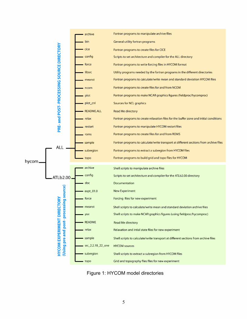
Your HYCOM directory is now built as in Figure 1. The next step is the compilation of the ALL directory. This will make the pre- and post processing source available.

5

Figure 1: HYCOM model directories

6

a. ALL directory (Pre and post processing source directory)

In this directory, you will find all the sources (written in FORTRAN) used in the shell scripts of the ATLb2.00 directory. These FORTRAN functions are able to manipulate all the kind of files needed or given by the HYCOM model.

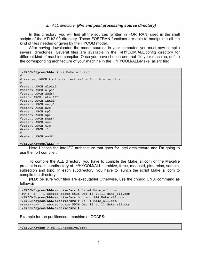
After having downloaded the model sources in your computer, you must now compile several directories. Several files are available in the ~/HYCOM/ALL/config directory for different kind of machine compiler. Once you have chosen one that fits your machine, define the corresponding architecture of your machine in the ~/HYCOM/ALL/Make_all.src file:

~/HYCOM/hycom/ALL/ > vi Make_all.src # # --- set ARCH to the correct value for this machine. # #setenv ARCH alphaL #setenv ARCH alpha #setenv ARCH amd64 setenv ARCH intelIFC #setenv ARCH intel #setenv ARCH macg5 #setenv ARCH o2k #setenv ARCH sp3 #setenv ARCH sp4 #setenv ARCH sun64 #setenv ARCH sun #setenv ARCH t3e #setenv ARCH x1 # #setenv ARCH amd64 ~/HYCOM/hycom/ALL/ >

Here I chose the intelIFC architecture that goes for Intel architecture and I’m going to use the ifort compiler.

To compile the ALL directory, you have to compile the Make_all.com or the Makefile

present in each subdirectory of ~/HYCOM/ALL : archive, force, meanstd, plot, relax, sample, subregion and topo. In each subdirectory, you have to launch the script Make_all.com to compile the directory.

(N.B: be sure your files are executable! Otherwise, use the chmod UNIX command as follows): ~/HYCOM/hycom/ALL/archive/src > ls –l Make_all.com -rw-r--r-- 1 abozec coaps 5536 Dec 18 11:11 Make_all.com ~/HYCOM/hycom/ALL/archive/src > chmod 744 Make_all.com ~/HYCOM/hycom/ALL/archive/src > ls –l Make_all.com -rwxr--r-- 1 abozec coaps 5536 Dec 18 11:11 Make_all.com ~/HYCOM/hycom/ALL/archive/src > Example for the pacificocean machine at COAPS: ~/HYCOM/hycom > cd ALL/archive/src/

7

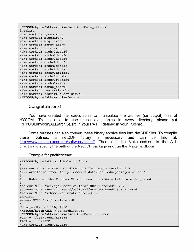
~/HYCOM/hycom/ALL/archive/src > ./Make_all.com intelIFC Make worked: hycomarchv Make worked: micomarchv Make worked: mrgl_archv Make worked: remap_archv Make worked: trim_archv Make worked: archv2data2d Make worked: archm2data2d Make worked: archv2data2t Make worked: archv2data3z Make worked: archm2data3z Make worked: archv2datasf Make worked: archv2datasfl Make worked: archv2ncombc Make worked: archv2restart Make worked: archm2restart Make worked: remap_archv Make worked: restart2archv Make worked: restart2archv_sig2a ~/HYCOM/hycom/ALL/archive/src >

Congratulations! You have created the executables to manipulate the archive (i.e output) files of

HYCOM. To be able to use these executables in every directory, please put ~/HYCOM/hycom/ALL/archive/src in your PATH (defined in your ~/.cshrc).

Some routines can also convert these binary archive files into NetCDF files. To compile

these routines, a netCDF library is necessary and can be find at: http://www.unidata.ucar.edu/software/netcdf/. Then, edit the Make_ncdf.src in the ALL directory to specify the path of the NetCDF package and run the Make_ncdf.com.

Example for pacificocean:

~/HYCOM/hycom/ALL > vi Make_ncdf.src # #--- set NCDF to the root directory for netCDF version 3.5. #--- available from: #http://www.unidata.ucar.edu/packages/netcdf/ # #--- Note that the Fortran 90 routines and module files are #required. # #setenv NCDF /net/ajax/scrf/wallcraf/NETCDF/netcdf-3.5.0 #setenv NCDF /net/ajax/scrf/wallcraf/NETCDF/netcdf-3.5.1-intel #setenv NCDF /u/home/wallcraf/netcdf-3.5.0 #PACIFIC setenv NCDF /usr/local/netcdf ~ "Make_ncdf.src" 11L, 426C ~/HYCOM/hycom/ALL > cd archive/src ~/HYCOM/hycom/ALL/archive/src > ./Make_ncdf.com NCDF = /usr/local/netcdf ARCH = intelIFC Make worked: archv2ncdf2d

8

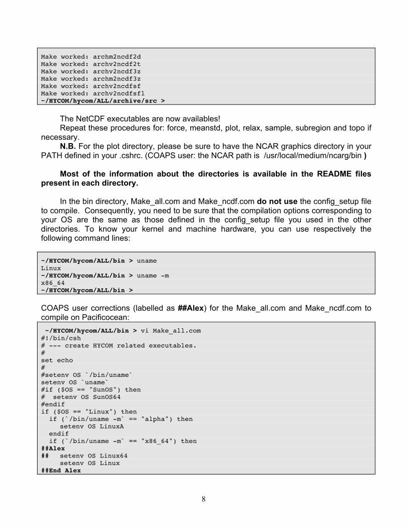
Make worked: archm2ncdf2d Make worked: archv2ncdf2t Make worked: archv2ncdf3z Make worked: archm2ncdf3z Make worked: archv2ncdfsf Make worked: archv2ncdfsfl ~/HYCOM/hycom/ALL/archive/src >

The NetCDF executables are now availables! Repeat these procedures for: force, meanstd, plot, relax, sample, subregion and topo if

necessary. N.B. For the plot directory, please be sure to have the NCAR graphics directory in your

PATH defined in your .cshrc. (COAPS user: the NCAR path is /usr/local/medium/ncarg/bin ) Most of the information about the directories is available in the README files

present in each directory. In the bin directory, Make_all.com and Make_ncdf.com do not use the config_setup file

to compile. Consequently, you need to be sure that the compilation options corresponding to your OS are the same as those defined in the config_setup file you used in the other directories. To know your kernel and machine hardware, you can use respectively the following command lines:

~/HYCOM/hycom/ALL/bin > uname Linux ~/HYCOM/hycom/ALL/bin > uname -m x86_64 ~/HYCOM/hycom/ALL/bin > COAPS user corrections (labelled as ##Alex) for the Make_all.com and Make_ncdf.com to compile on Pacificocean: ~/HYCOM/hycom/ALL/bin > vi Make_all.com #!/bin/csh # --- create HYCOM related executables. # set echo # #setenv OS `/bin/uname` setenv OS `uname` #if ($OS == "SunOS") then # setenv OS SunOS64 #endif if ($OS == "Linux") then if (`/bin/uname -m` == "alpha") then setenv OS LinuxA endif if (`/bin/uname -m` == "x86_64") then ##Alex ## setenv OS Linux64 setenv OS Linux ##End Alex

9

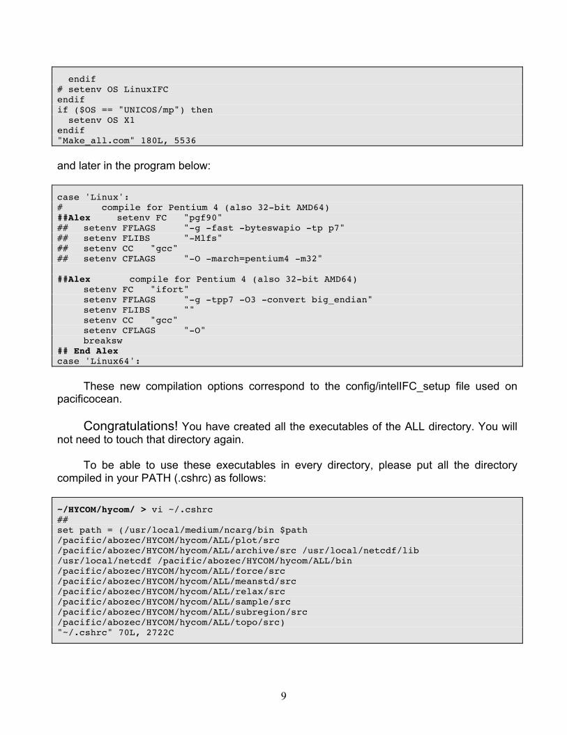
endif # setenv OS LinuxIFC endif if ($OS == "UNICOS/mp") then setenv OS X1 endif "Make_all.com" 180L, 5536 and later in the program below: case 'Linux': # compile for Pentium 4 (also 32-bit AMD64) ##Alex setenv FC "pgf90" ## setenv FFLAGS "-g -fast -byteswapio -tp p7" ## setenv FLIBS "-Mlfs" ## setenv CC "gcc" ## setenv CFLAGS "-O -march=pentium4 -m32" ##Alex compile for Pentium 4 (also 32-bit AMD64) setenv FC "ifort" setenv FFLAGS "-g -tpp7 -O3 -convert big_endian" setenv FLIBS "" setenv CC "gcc" setenv CFLAGS "-O" breaksw ## End Alex case 'Linux64':

These new compilation options correspond to the config/intelIFC_setup file used on pacificocean.

Congratulations! You have created all the executables of the ALL directory. You will

not need to touch that directory again. To be able to use these executables in every directory, please put all the directory

compiled in your PATH (.cshrc) as follows:

~/HYCOM/hycom/ > vi ~/.cshrc ## set path = (/usr/local/medium/ncarg/bin $path /pacific/abozec/HYCOM/hycom/ALL/plot/src /pacific/abozec/HYCOM/hycom/ALL/archive/src /usr/local/netcdf/lib /usr/local/netcdf /pacific/abozec/HYCOM/hycom/ALL/bin /pacific/abozec/HYCOM/hycom/ALL/force/src /pacific/abozec/HYCOM/hycom/ALL/meanstd/src /pacific/abozec/HYCOM/hycom/ALL/relax/src /pacific/abozec/HYCOM/hycom/ALL/sample/src /pacific/abozec/HYCOM/hycom/ALL/subregion/src /pacific/abozec/HYCOM/hycom/ALL/topo/src) "~/.cshrc" 70L, 2722C

10

b. ATL directory/Atlantic configuration of HYCOM (Working Directory)

In this directory, you will find the source of HYCOM model, the input and output files directory, the run directory and examples of visualisation shell script (See figure 1).

Most of the information about the directories is available in the README files present in each directory.

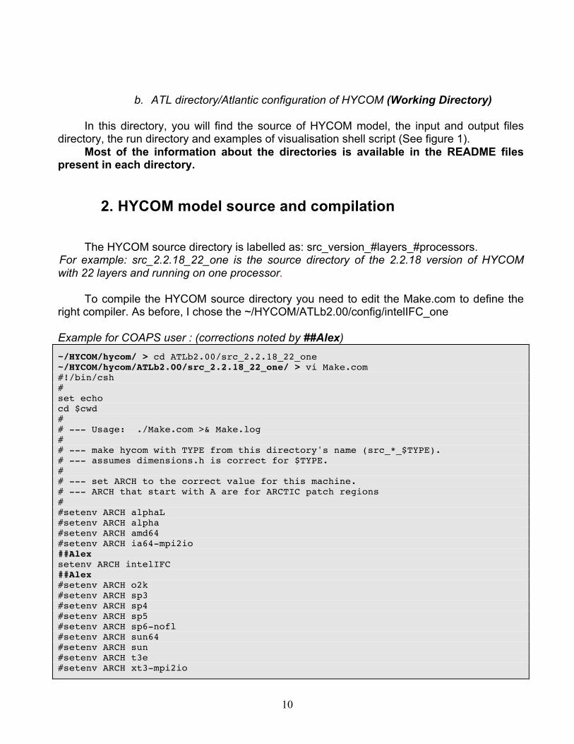
2. HYCOM model source and compilation

The HYCOM source directory is labelled as: src_version_#layers_#processors. For example: src_2.2.18_22_one is the source directory of the 2.2.18 version of HYCOM with 22 layers and running on one processor.

To compile the HYCOM source directory you need to edit the Make.com to define the

right compiler. As before, I chose the ~/HYCOM/ATLb2.00/config/intelIFC_one

Example for COAPS user : (corrections noted by ##Alex) ~/HYCOM/hycom/ > cd ATLb2.00/src_2.2.18_22_one ~/HYCOM/hycom/ATLb2.00/src_2.2.18_22_one/ > vi Make.com #!/bin/csh # set echo cd $cwd # # --- Usage: ./Make.com >& Make.log # # --- make hycom with TYPE from this directory's name (src_*_$TYPE). # --- assumes dimensions.h is correct for $TYPE. # # --- set ARCH to the correct value for this machine. # --- ARCH that start with A are for ARCTIC patch regions # #setenv ARCH alphaL #setenv ARCH alpha #setenv ARCH amd64 #setenv ARCH ia64-mpi2io ##Alex setenv ARCH intelIFC ##Alex #setenv ARCH o2k #setenv ARCH sp3 #setenv ARCH sp4 #setenv ARCH sp5 #setenv ARCH sp6-nofl #setenv ARCH sun64 #setenv ARCH sun #setenv ARCH t3e #setenv ARCH xt3-mpi2io

11

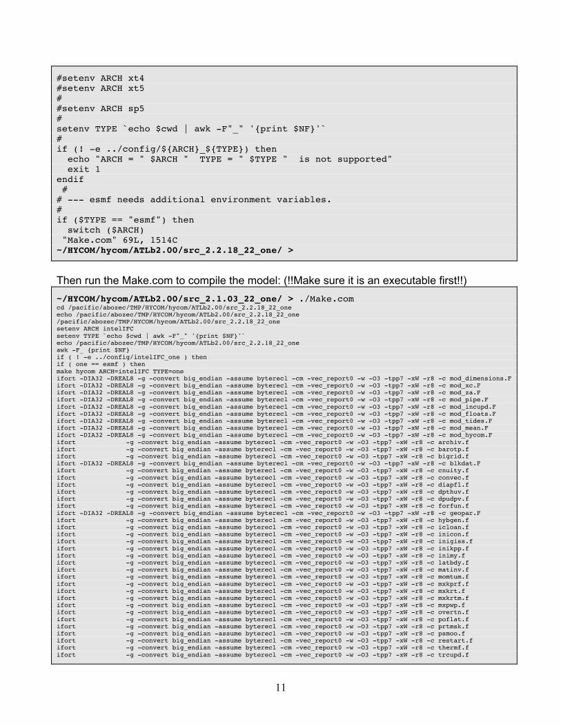
#setenv ARCH xt4 #setenv ARCH xt5 # #setenv ARCH sp5 # setenv TYPE `echo $cwd | awk -F"_" '{print $NF}'` # if (! -e ../config/${ARCH}_${TYPE}) then echo "ARCH = " $ARCH " TYPE = " $TYPE " is not supported" exit 1 endif # # --- esmf needs additional environment variables. # if ($TYPE == "esmf") then switch ($ARCH) "Make.com" 69L, 1514C ~/HYCOM/hycom/ATLb2.00/src_2.2.18_22_one/ >

Then run the Make.com to compile the model: (!!Make sure it is an executable first!!) ~/HYCOM/hycom/ATLb2.00/src_2.1.03_22_one/ > ./Make.com cd /pacific/abozec/TMP/HYCOM/hycom/ATLb2.00/src_2.2.18_22_one echo /pacific/abozec/TMP/HYCOM/hycom/ATLb2.00/src_2.2.18_22_one /pacific/abozec/TMP/HYCOM/hycom/ATLb2.00/src_2.2.18_22_one setenv ARCH intelIFC setenv TYPE `echo $cwd | awk -F"_" '{print $NF}'` echo /pacific/abozec/TMP/HYCOM/hycom/ATLb2.00/src_2.2.18_22_one awk -F_ {print $NF} if ( ! -e ../config/intelIFC_one ) then if ( one == esmf ) then make hycom ARCH=intelIFC TYPE=one ifort -DIA32 -DREAL8 -g -convert big_endian -assume byterecl -cm -vec_report0 -w -O3 -tpp7 -xW -r8 -c mod_dimensions.F ifort -DIA32 -DREAL8 -g -convert big_endian -assume byterecl -cm -vec_report0 -w -O3 -tpp7 -xW -r8 -c mod_xc.F ifort -DIA32 -DREAL8 -g -convert big_endian -assume byterecl -cm -vec_report0 -w -O3 -tpp7 -xW -r8 -c mod_za.F ifort -DIA32 -DREAL8 -g -convert big_endian -assume byterecl -cm -vec_report0 -w -O3 -tpp7 -xW -r8 -c mod_pipe.F ifort -DIA32 -DREAL8 -g -convert big_endian -assume byterecl -cm -vec_report0 -w -O3 -tpp7 -xW -r8 -c mod_incupd.F ifort -DIA32 -DREAL8 -g -convert big_endian -assume byterecl -cm -vec_report0 -w -O3 -tpp7 -xW -r8 -c mod_floats.F ifort -DIA32 -DREAL8 -g -convert big_endian -assume byterecl -cm -vec_report0 -w -O3 -tpp7 -xW -r8 -c mod_tides.F ifort -DIA32 -DREAL8 -g -convert big_endian -assume byterecl -cm -vec_report0 -w -O3 -tpp7 -xW -r8 -c mod_mean.F ifort -DIA32 -DREAL8 -g -convert big_endian -assume byterecl -cm -vec_report0 -w -O3 -tpp7 -xW -r8 -c mod_hycom.F ifort -g -convert big_endian -assume byterecl -cm -vec_report0 -w -O3 -tpp7 -xW -r8 -c archiv.f ifort -g -convert big_endian -assume byterecl -cm -vec_report0 -w -O3 -tpp7 -xW -r8 -c barotp.f ifort -g -convert big_endian -assume byterecl -cm -vec_report0 -w -O3 -tpp7 -xW -r8 -c bigrid.f ifort -DIA32 -DREAL8 -g -convert big_endian -assume byterecl -cm -vec_report0 -w -O3 -tpp7 -xW -r8 -c blkdat.F ifort -g -convert big_endian -assume byterecl -cm -vec_report0 -w -O3 -tpp7 -xW -r8 -c cnuity.f ifort -g -convert big_endian -assume byterecl -cm -vec_report0 -w -O3 -tpp7 -xW -r8 -c convec.f ifort -g -convert big_endian -assume byterecl -cm -vec_report0 -w -O3 -tpp7 -xW -r8 -c diapfl.f ifort -g -convert big_endian -assume byterecl -cm -vec_report0 -w -O3 -tpp7 -xW -r8 -c dpthuv.f ifort -g -convert big_endian -assume byterecl -cm -vec_report0 -w -O3 -tpp7 -xW -r8 -c dpudpv.f ifort -g -convert big_endian -assume byterecl -cm -vec_report0 -w -O3 -tpp7 -xW -r8 -c forfun.f ifort -DIA32 -DREAL8 -g -convert big_endian -assume byterecl -cm -vec_report0 -w -O3 -tpp7 -xW -r8 -c geopar.F ifort -g -convert big_endian -assume byterecl -cm -vec_report0 -w -O3 -tpp7 -xW -r8 -c hybgen.f ifort -g -convert big_endian -assume byterecl -cm -vec_report0 -w -O3 -tpp7 -xW -r8 -c icloan.f ifort -g -convert big_endian -assume byterecl -cm -vec_report0 -w -O3 -tpp7 -xW -r8 -c inicon.f ifort -g -convert big_endian -assume byterecl -cm -vec_report0 -w -O3 -tpp7 -xW -r8 -c inigiss.f ifort -g -convert big_endian -assume byterecl -cm -vec_report0 -w -O3 -tpp7 -xW -r8 -c inikpp.f ifort -g -convert big_endian -assume byterecl -cm -vec_report0 -w -O3 -tpp7 -xW -r8 -c inimy.f ifort -g -convert big_endian -assume byterecl -cm -vec_report0 -w -O3 -tpp7 -xW -r8 -c latbdy.f ifort -g -convert big_endian -assume byterecl -cm -vec_report0 -w -O3 -tpp7 -xW -r8 -c matinv.f ifort -g -convert big_endian -assume byterecl -cm -vec_report0 -w -O3 -tpp7 -xW -r8 -c momtum.f ifort -g -convert big_endian -assume byterecl -cm -vec_report0 -w -O3 -tpp7 -xW -r8 -c mxkprf.f ifort -g -convert big_endian -assume byterecl -cm -vec_report0 -w -O3 -tpp7 -xW -r8 -c mxkrt.f ifort -g -convert big_endian -assume byterecl -cm -vec_report0 -w -O3 -tpp7 -xW -r8 -c mxkrtm.f ifort -g -convert big_endian -assume byterecl -cm -vec_report0 -w -O3 -tpp7 -xW -r8 -c mxpwp.f ifort -g -convert big_endian -assume byterecl -cm -vec_report0 -w -O3 -tpp7 -xW -r8 -c overtn.f ifort -g -convert big_endian -assume byterecl -cm -vec_report0 -w -O3 -tpp7 -xW -r8 -c poflat.f ifort -g -convert big_endian -assume byterecl -cm -vec_report0 -w -O3 -tpp7 -xW -r8 -c prtmsk.f ifort -g -convert big_endian -assume byterecl -cm -vec_report0 -w -O3 -tpp7 -xW -r8 -c psmoo.f ifort -g -convert big_endian -assume byterecl -cm -vec_report0 -w -O3 -tpp7 -xW -r8 -c restart.f ifort -g -convert big_endian -assume byterecl -cm -vec_report0 -w -O3 -tpp7 -xW -r8 -c thermf.f ifort -g -convert big_endian -assume byterecl -cm -vec_report0 -w -O3 -tpp7 -xW -r8 -c trcupd.f

12

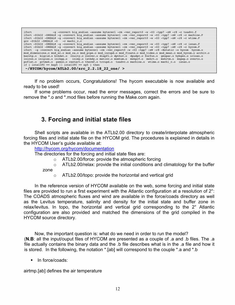
ifort -g -convert big_endian -assume byterecl -cm -vec_report0 -w -O3 -tpp7 -xW -r8 -c tsadvc.f ifort -DIA32 -DREAL8 -g -convert big_endian -assume byterecl -cm -vec_report0 -w -O3 -tpp7 -xW -r8 -c machine.F ifort -DIA32 -DREAL8 -g -convert big_endian -assume byterecl -cm -vec_report0 -w -O3 -tpp7 -xW -r8 -c wtime.F gcc -DIA32 -DREAL8 -O -c machi_c.c ifort -DIA32 -DREAL8 -g -convert big_endian -assume byterecl -cm -vec_report0 -w -O3 -tpp7 -xW -r8 -c isnan.F ifort -DIA32 -DREAL8 -g -convert big_endian -assume byterecl -cm -vec_report0 -w -O3 -tpp7 -xW -r8 -c hycom.F ifort -g -convert big_endian -assume byterecl -cm -vec_report0 -w -O3 -tpp7 -xW -r8 -Bstatic -o hycom hycom.o mod_dimensions.o mod_xc.o mod_za.o mod_pipe.o mod_incupd.o mod_floats.o mod_tides.o mod_mean.o mod_hycom.o archiv.o barotp.o bigrid.o blkdat.o cnuity.o convec.o diapfl.o dpthuv.o dpudpv.o forfun.o geopar.o hybgen.o icloan.o inicon.o inigiss.o inikpp.o inimy.o latbdy.o matinv.o momtum.o mxkprf.o mxkrt.o mxkrtm.o mxpwp.o overtn.o poflat.o prtmsk.o psmoo.o restart.o thermf.o trcupd.o tsadvc.o machine.o wtime.o machi_c.o isnan.o if ( intelIFC == Asp5 || intelIFC == sp5 ) then

~/HYCOM/hycom/ATLb2.00/src_2.2.18_22_one/ >

If no problem occurs, Congratulations! The hycom executable is now available and

ready to be used! If some problems occur, read the error messages, correct the errors and be sure to

remove the *.o and *.mod files before running the Make.com again.

3. Forcing and initial state files

Shell scripts are available in the ATLb2.00 directory to create/interpolate atmospheric forcing files and initial state file on the HYCOM grid. The procedures is explained in details in the HYCOM User’s guide available at:

http://hycom.org/hycom/documentation The directories for the forcing and initial state files are:

o ATLb2.00/force: provide the atmospheric forcing o ATLb2.00/relax: provide the initial conditions and climatology for the buffer

zone o ATLb2.00/topo: provide the horizontal and vertical grid

In the reference version of HYCOM available on the web, some forcing and initial state

files are provided to run a first experiment with the Atlantic configuration at a resolution of 2°: The COADS atmospheric fluxes and wind are available in the force/coads directory as well as the Levitus temperature, salinity and density for the initial state and buffer zone in relax/levitus. In topo, the horizontal and vertical grid corresponding to the 2° Atlantic configuration are also provided and matched the dimensions of the grid compiled in the HYCOM source directory.

Now, the important question is: what do we need in order to run the model? (N.B: all the input/ouput files of HYCOM are presented as a couple of .a and .b files. The .a file actually contains the binary data and the .b file describes what is in the .a file and how it is stored. In the following, the notation *.[ab] will correspond to the couple *.a and *.b

In force/coads:

airtmp.[ab] defines the air temperature

13

surtmp.[ab] defines the surface temperature seatmp.[ab] defines the sea temperature wndspd.[ab] defines the windspeed taunwd.[ab] defines the meridional windstress tauewd.[ab] defines the zonal windstress shwflx.[ab] defines the shortwave flux radflx.[ab] defines the radiative flux precip.[ab] defines the precipitation vapmix.[ab] defines the evaporation

In topo:

regional.grid.[ab] defines the horizontal grid of your configuration depth_ATLb2.00_01.[ab] defines the vertical grid of your configuration

In relax/nb_expt:

relax_tem.[ab] defines the temperature of the initial state and of the buffer zones relax_sal.[ab] defines the salinity of the initial state and of the buffer zones relax_int.[ab] defines the depths of the layer interface of the initial state and of the buffer zones relax_rmu.[ab] defines the locations of the buffer zones and the relaxation factor in each of them. (N.B. The number of the experiment (nb_expt) is defined as explained in N.B. section 4. This directory must be created in relax directory for each experiment!) Most of the information about the directories is available in the README files present in each directory.

4. How to run the model

In this section, we present the method to build and run a new experiment. Please keep

in mind that some parameters can change depending of the HYCOM source version used. Several examples of experiments are available in the ATLb2.00 directory: expt_01.5 that uses 2.1.03 HYCOM version, expt_01.6 that use the 2.1.34 version and finally expt_02.0 that uses the latest version 2.2.18. In each directory, you will find the shell scripts needed to run the model. Here we will create a new experiment based on expt_02.0. NB: please, follow some rules of notation:

14

A new experiment directory is defined as: expt_XX.Y such as expt_01.5 (XX=01 and Y=5).

The number of the experiment (nb_expt) is then: XXY such as 015. A new directory, nb_expt, must be created in relax for each experiment!

The most important files in the expt_XX.Y directory:

blkdat.input : parameters of the experiment (namelist) nb_expty001.limits: Time limits of the run (XXYyddd.limits with ddd the beginning year

of the run, here ddd=001) XXY.com: Shell script allowing to run the model on different OS

To create a new experiment, no need to copy all these files, just follow the following instructions:

Create a new directory in ATLb2.00: ~/HYCOM/hycom/ATLb2.00/ > mkdir expt_01.7 ~/HYCOM/hycom/ATLb2.00/ >

Copy the new_expt.com shell script from expt_02.0/ to expt_01.7/

~/HYCOM/hycom/ATLb2.00/ > cp expt_02.0/new_expt.com expt_01.7 ~/HYCOM/hycom/ATLb2.00/ > cd expt_01.7 ~/HYCOM/hycom/ATLb2.00/expt_01.7 >

Edit the DO, O, DN and N of new_expt.com as follows. This script will automatically

copy and edit with the right number of experiment all the scripts that you need into this new experiment directory.

~/HYCOM/hycom/ATLb2.00/expt_01.7 > vi new_expt.com #!/bin/csh set echo # # --- build new expt files from old. # --- some files will need additional manual editing. # # DO = old experiment directory name # O = old experiment number # DN = new experiment directory name # N = new experiment number # R = region name. # setenv DO expt_2.0 setenv O 020 setenv DN expt_01.7 setenv N 017 setenv R ATLb2.00 # "new_expt.com" 40L, 907C

15

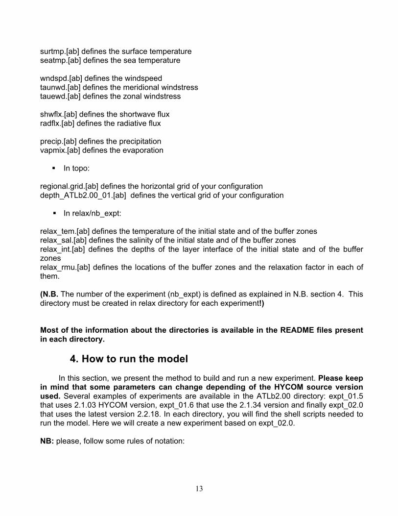
~/HYCOM/hycom/ATLb2.00/expt_01.7 > ./new_expt.com setenv DO expt_02.0 setenv O 020 setenv DN expt_01.7 setenv N 017 setenv R ATLb2.00 setenv RO ATLb2.00 setenv D ../../ATLb2.00/expt_02.0 foreach t ( .com W.com F.com P.com y001.limits cod.com lsf.com nqs.com rll.com grd.com ) sed -e s/setenv E .*020.*/setenv E 017/g -e s/expt_02.0/expt_01.7/g -e s/ATLb2.00/ATLb2.00/g ../../ATLb2.00/expt_02.0/020.com end sed -e s/setenv E .*020.*/setenv E 017/g -e s/expt_02.0/expt_01.7/g -e s/ATLb2.00/ATLb2.00/g ../../ATLb2.00/expt_02.0/020W.com end sed -e s/setenv E .*020.*/setenv E 017/g -e s/expt_02.0/expt_01.7/g -e s/ATLb2.00/ATLb2.00/g ../../ATLb2.00/expt_02.0/020F.com end sed -e s/setenv E .*020.*/setenv E 017/g -e s/expt_02.0/expt_01.7/g -e s/ATLb2.00/ATLb2.00/g ../../ATLb2.00/expt_02.0/020P.com end sed -e s/setenv E .*020.*/setenv E 017/g -e s/expt_02.0/expt_01.7/g -e s/ATLb2.00/ATLb2.00/g ../../ATLb2.00/expt_02.0/020y001.limits end sed -e s/setenv E .*020.*/setenv E 017/g -e s/expt_02.0/expt_01.7/g -e s/ATLb2.00/ATLb2.00/g ../../ATLb2.00/expt_02.0/020cod.com end sed -e s/setenv E .*020.*/setenv E 017/g -e s/expt_02.0/expt_01.7/g -e s/ATLb2.00/ATLb2.00/g ../../ATLb2.00/expt_02.0/020lsf.com end sed -e s/setenv E .*020.*/setenv E 017/g -e s/expt_02.0/expt_01.7/g -e s/ATLb2.00/ATLb2.00/g ../../ATLb2.00/expt_02.0/020nqs.com end sed -e s/setenv E .*020.*/setenv E 017/g -e s/expt_02.0/expt_01.7/g -e s/ATLb2.00/ATLb2.00/g ../../ATLb2.00/expt_02.0/020rll.com end sed -e s/setenv E .*020.*/setenv E 017/g -e s/expt_02.0/expt_01.7/g -e s/ATLb2.00/ATLb2.00/g ../../ATLb2.00/expt_02.0/020grd.com end cp -i ../../ATLb2.00/expt_02.0/020.awk 017.awk cp -i ../../ATLb2.00/expt_02.0/blkdat.input ../../ATLb2.00/expt_02.0/ports.input . cp -i ../../ATLb2.00/expt_02.0/dummyA.com ../../ATLb2.00/expt_02.0/dummyB.com ../../ATLb2.00/expt_02.0/dummyC.com ../../ATLb2.00/expt_02.0/dummyD.com . mlist 001 020 1 cp -i LIST LIST++ mkdir data ~/HYCOM/hycom/ATLb2.00/expt_01.7 > ls 017.awk 017F.com 017nqs.com 017W.com data dummyC.com LIST++ 017cod.com 017grd.com 017P.com 017y001.limits dummyA.com dummyD.com new_expt.com 017.com 017lsf.com 017rll.com blkdat.input dummyB.com LIST ports.input ~/HYCOM/hycom/ATLb2.00/expt_01.7 >

You have now all the files needed to run an experiment!! Let’s go: For a climatological run:

Check or Edit the 017.com to define: o The version of HYCOM used o The path of the HYCOM source directory o The topography used o The number of layer of the configuration o The path of the outputs directory

Lines between the two ##Alex have to be edited by the user. (Warning: the following lines are not at the beginning of the 017.com script)

16

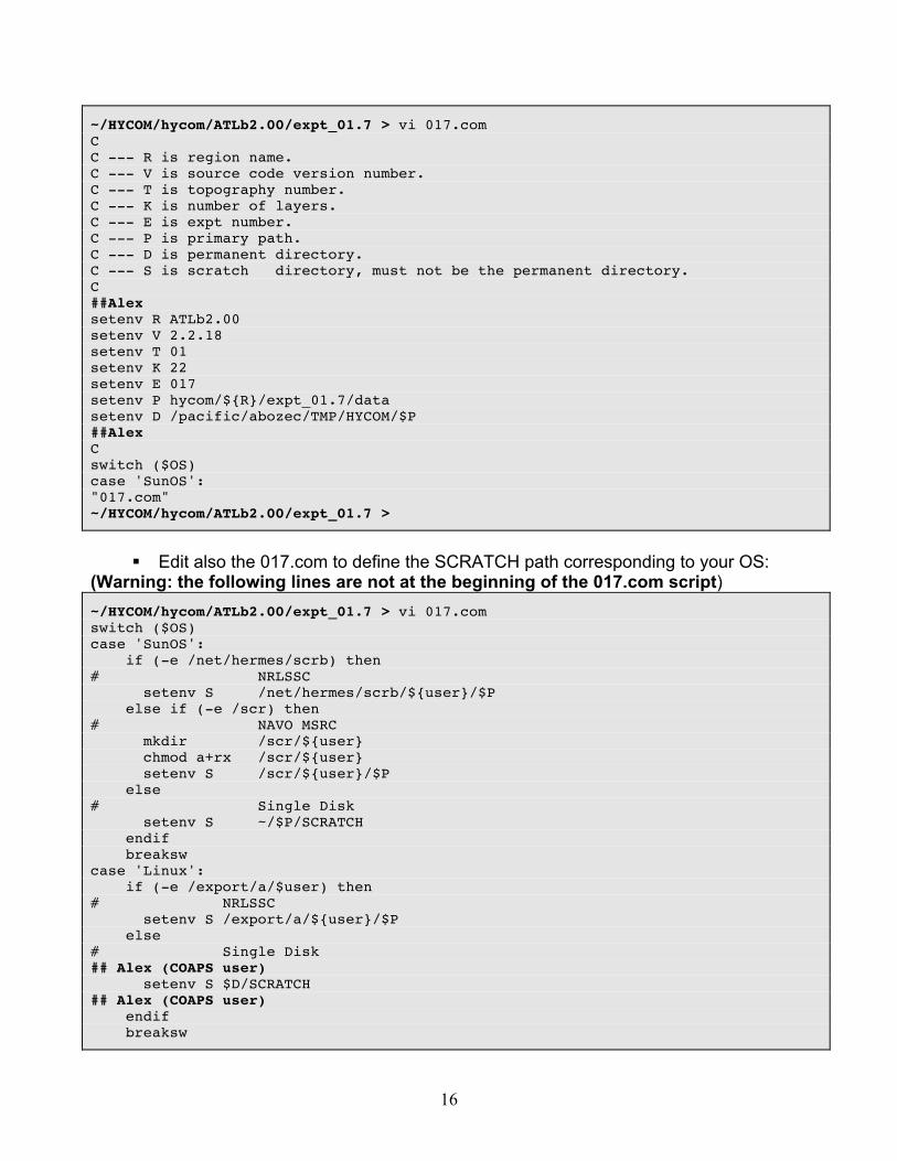
~/HYCOM/hycom/ATLb2.00/expt_01.7 > vi 017.com C C --- R is region name. C --- V is source code version number. C --- T is topography number. C --- K is number of layers. C --- E is expt number. C --- P is primary path. C --- D is permanent directory. C --- S is scratch directory, must not be the permanent directory. C ##Alex setenv R ATLb2.00 setenv V 2.2.18 setenv T 01 setenv K 22 setenv E 017 setenv P hycom/${R}/expt_01.7/data setenv D /pacific/abozec/TMP/HYCOM/$P ##Alex C switch ($OS) case 'SunOS': "017.com" ~/HYCOM/hycom/ATLb2.00/expt_01.7 >

Edit also the 017.com to define the SCRATCH path corresponding to your OS:

(Warning: the following lines are not at the beginning of the 017.com script) ~/HYCOM/hycom/ATLb2.00/expt_01.7 > vi 017.com switch ($OS) case 'SunOS': if (-e /net/hermes/scrb) then # NRLSSC setenv S /net/hermes/scrb/${user}/$P else if (-e /scr) then # NAVO MSRC mkdir /scr/${user} chmod a+rx /scr/${user} setenv S /scr/${user}/$P else # Single Disk setenv S ~/$P/SCRATCH endif breaksw case 'Linux': if (-e /export/a/$user) then # NRLSSC setenv S /export/a/${user}/$P else # Single Disk ## Alex (COAPS user) setenv S $D/SCRATCH ## Alex (COAPS user) endif breaksw

17

"017.com" ~/HYCOM/hycom/ATLb2.00/expt_01.7 >

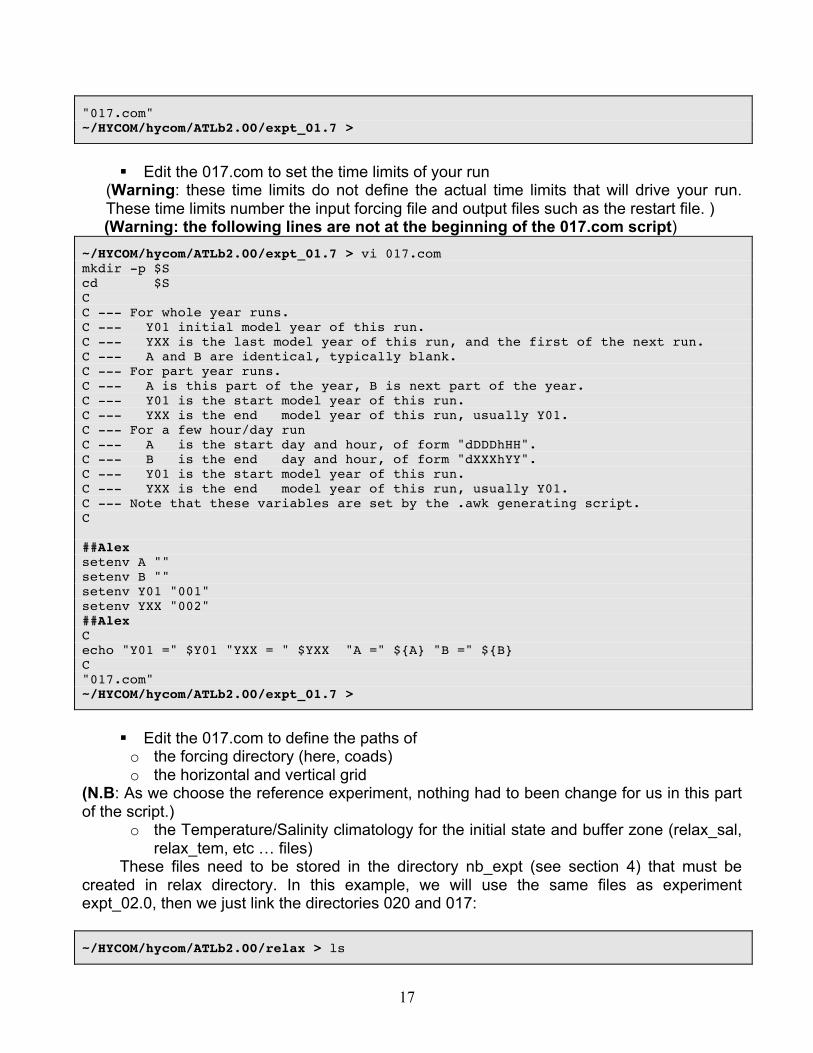
Edit the 017.com to set the time limits of your run

(Warning: these time limits do not define the actual time limits that will drive your run. These time limits number the input forcing file and output files such as the restart file. )

(Warning: the following lines are not at the beginning of the 017.com script) ~/HYCOM/hycom/ATLb2.00/expt_01.7 > vi 017.com mkdir -p $S cd $S C C --- For whole year runs. C --- Y01 initial model year of this run. C --- YXX is the last model year of this run, and the first of the next run. C --- A and B are identical, typically blank. C --- For part year runs. C --- A is this part of the year, B is next part of the year. C --- Y01 is the start model year of this run. C --- YXX is the end model year of this run, usually Y01. C --- For a few hour/day run C --- A is the start day and hour, of form "dDDDhHH". C --- B is the end day and hour, of form "dXXXhYY". C --- Y01 is the start model year of this run. C --- YXX is the end model year of this run, usually Y01. C --- Note that these variables are set by the .awk generating script. C ##Alex setenv A "" setenv B "" setenv Y01 "001" setenv YXX "002" ##Alex C echo "Y01 =" $Y01 "YXX = " $YXX "A =" ${A} "B =" ${B} C "017.com" ~/HYCOM/hycom/ATLb2.00/expt_01.7 >

Edit the 017.com to define the paths of o the forcing directory (here, coads) o the horizontal and vertical grid

(N.B: As we choose the reference experiment, nothing had to been change for us in this part of the script.)

o the Temperature/Salinity climatology for the initial state and buffer zone (relax_sal, relax_tem, etc … files)

These files need to be stored in the directory nb_expt (see section 4) that must be created in relax directory. In this example, we will use the same files as experiment expt_02.0, then we just link the directories 020 and 017:

~/HYCOM/hycom/ATLb2.00/relax > ls

18

010 012 013 015 016 999 levitus plot plot_save README.relax README.relax.plot README.relax.zonal ~/HYCOM/hycom/ATLb2.00/relax > ~/HYCOM/hycom/ATLb2.00/relax > ln –s 020 017 ~/HYCOM/hycom/ATLb2.00/relax > ls 010 012 013 015 016 017 999 levitus plot plot_save README.relax README.relax.plot README.relax.zonal ~/HYCOM/hycom/ATLb2.00/relax >

(N.B: Please refer to the HYCOM User’s guide for the method used to create these HYCOM interpolated grid files from a regular grid climatology like Levitus.)

We can now come back to our experiment directory:

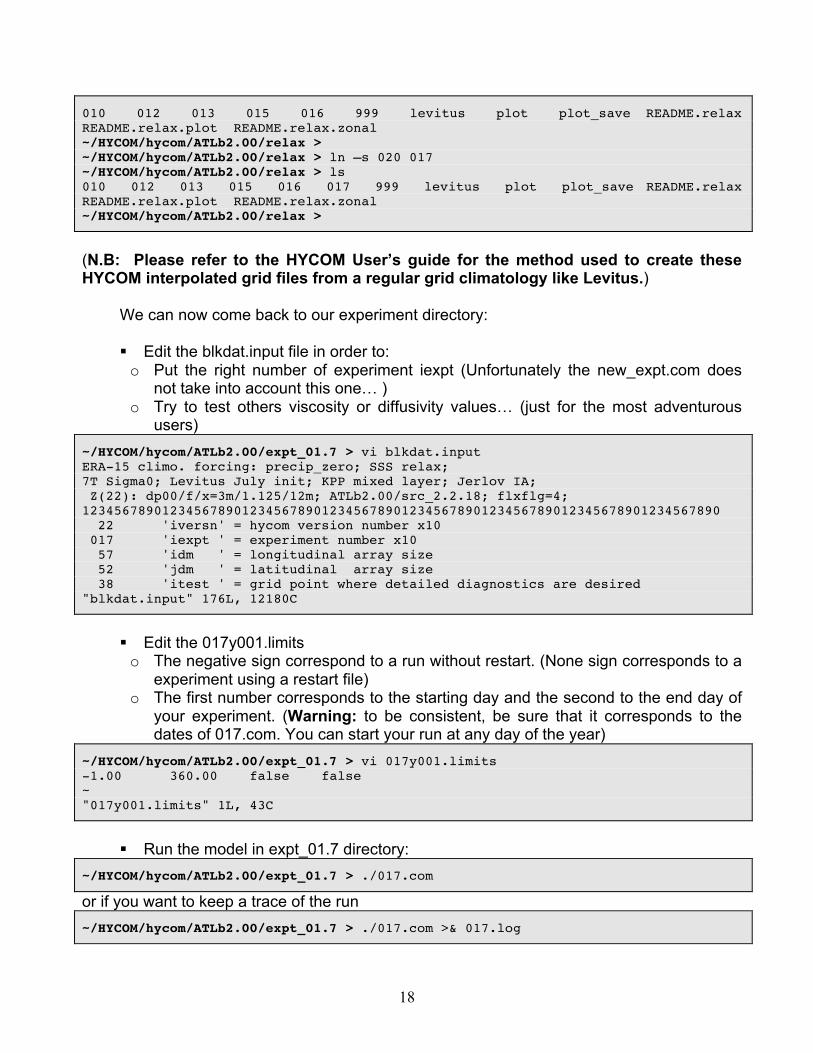
Edit the blkdat.input file in order to: o Put the right number of experiment iexpt (Unfortunately the new_expt.com does

not take into account this one… ) o Try to test others viscosity or diffusivity values… (just for the most adventurous

users) ~/HYCOM/hycom/ATLb2.00/expt_01.7 > vi blkdat.input ERA-15 climo. forcing: precip_zero; SSS relax; 7T Sigma0; Levitus July init; KPP mixed layer; Jerlov IA; Z(22): dp00/f/x=3m/1.125/12m; ATLb2.00/src_2.2.18; flxflg=4; 12345678901234567890123456789012345678901234567890123456789012345678901234567890 22 'iversn' = hycom version number x10 017 'iexpt ' = experiment number x10 57 'idm ' = longitudinal array size 52 'jdm ' = latitudinal array size 38 'itest ' = grid point where detailed diagnostics are desired "blkdat.input" 176L, 12180C

Edit the 017y001.limits o The negative sign correspond to a run without restart. (None sign corresponds to a

experiment using a restart file) o The first number corresponds to the starting day and the second to the end day of

your experiment. (Warning: to be consistent, be sure that it corresponds to the dates of 017.com. You can start your run at any day of the year)

~/HYCOM/hycom/ATLb2.00/expt_01.7 > vi 017y001.limits -1.00 360.00 false false ~ "017y001.limits" 1L, 43C

Run the model in expt_01.7 directory:

~/HYCOM/hycom/ATLb2.00/expt_01.7 > ./017.com

or if you want to keep a trace of the run ~/HYCOM/hycom/ATLb2.00/expt_01.7 > ./017.com >& 017.log

19

The output archives are put in the data/SCRATCH/tarv_ddd directory for instantaneous

outputs (ddd is 001 for our example), tarm_ddd for mean outputs and tare_ddd for ESMF outputs (From the ESMF coupler). The output archives are presented as *.a and *.b files. The results are stored in the *.a files while the description of these data are in the *.b corresponding files.

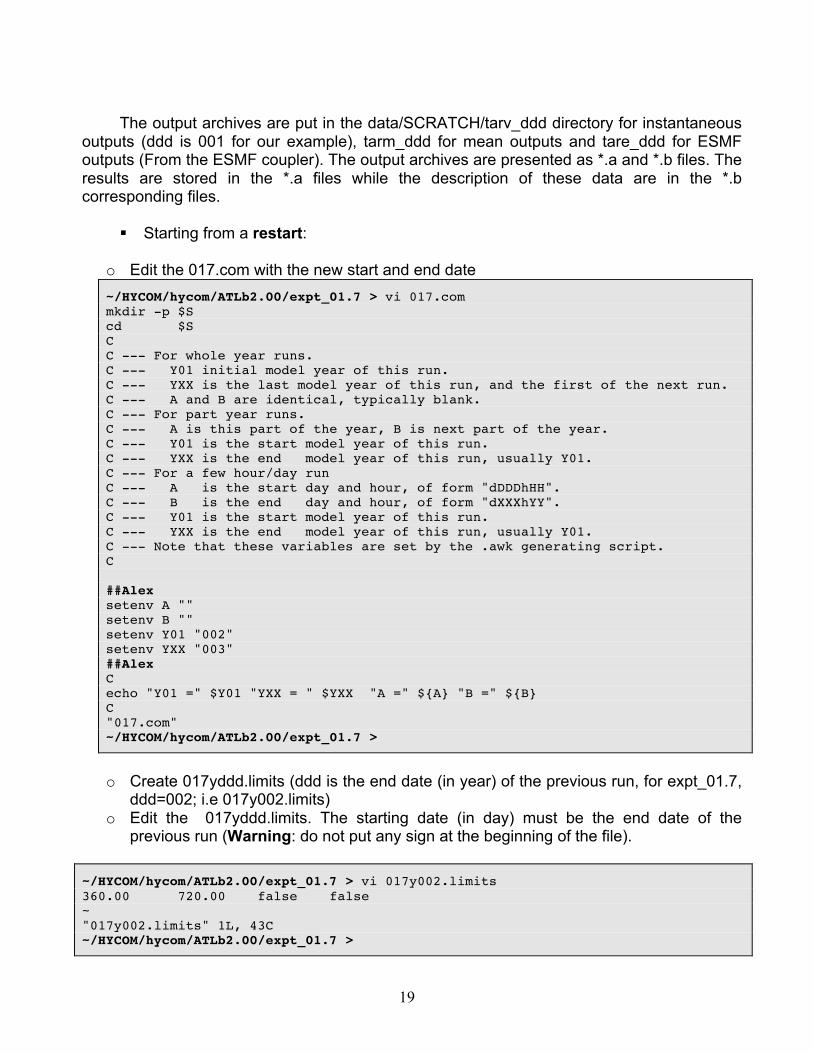
Starting from a restart:

o Edit the 017.com with the new start and end date ~/HYCOM/hycom/ATLb2.00/expt_01.7 > vi 017.com mkdir -p $S cd $S C C --- For whole year runs. C --- Y01 initial model year of this run. C --- YXX is the last model year of this run, and the first of the next run. C --- A and B are identical, typically blank. C --- For part year runs. C --- A is this part of the year, B is next part of the year. C --- Y01 is the start model year of this run. C --- YXX is the end model year of this run, usually Y01. C --- For a few hour/day run C --- A is the start day and hour, of form "dDDDhHH". C --- B is the end day and hour, of form "dXXXhYY". C --- Y01 is the start model year of this run. C --- YXX is the end model year of this run, usually Y01. C --- Note that these variables are set by the .awk generating script. C ##Alex setenv A "" setenv B "" setenv Y01 "002" setenv YXX "003" ##Alex C echo "Y01 =" $Y01 "YXX = " $YXX "A =" ${A} "B =" ${B} C "017.com" ~/HYCOM/hycom/ATLb2.00/expt_01.7 >

o Create 017yddd.limits (ddd is the end date (in year) of the previous run, for expt_01.7,

ddd=002; i.e 017y002.limits) o Edit the 017yddd.limits. The starting date (in day) must be the end date of the

previous run (Warning: do not put any sign at the beginning of the file).

~/HYCOM/hycom/ATLb2.00/expt_01.7 > vi 017y002.limits 360.00 720.00 false false ~ "017y002.limits" 1L, 43C ~/HYCOM/hycom/ATLb2.00/expt_01.7 >

20

o Run the model in expt_01.7/

~/HYCOM/hycom/ATLb2.00/expt_01.7 > ./017.com

5. HYCOM frequents error Pwall2 error: Generally happens when your climatology (relax files) are not in agreement with your topographic files. Solution: either make sure the relax files corresponds to your bathymetry or do: ~/HYCOM/hycom/ATLb2.00/expt_01.7/data/SCRATCH> touch relax.weird

21

6. How to visualize the result – NCAR graphics –

NCAR Graphics, a time-tested UNIX package, consists mainly of over two-dozen Fortran/C utilities for drawing contours, maps, vectors, streamlines, weather maps, surfaces, histograms, X/Y plots, annotations, and more.

Examples of plot script with NCAR graphic are given in ATLb2.00/plot directory. Two main routines using NCAR graphics have been developed for HYCOM:

fieldproc and hycomproc. (Warning: be sure that ALL/plot/src is in your path to use fieldproc and hycomproc)

a. fieldproc

!!!WARNING !!! fieldproc is used only for the 2D fields. If you try to use fieldproc to make a section plot you will have an error message. For sections or 3D fields use hycomproc (see section 5.b).

The command line for fieldproc is: ~/HYCOM/hycom/ATLb2.00/plot > fieldproc < depth.IN

or ~/HYCOM/hycom/ATLb2.00/plot > fp < depth.IN

You then obtain a postscript file named: gmeta1.ps fp and hp are some kind of aliases that can be used for respectively fieldproc and

hycomproc. Others aliases can be useful as hp2ps or fp2ps that named directly your postcript file as your shell script file. ~/HYCOM/hycom/ATLb2.00/plot > fp2ps depth.IN ~/HYCOM/hycom/ATLb2.00/plot > ls *.ps depth.ps ~/HYCOM/hycom/ATLb2.00/plot >

You just have to adapt or create your .IN files for your needs. In Appendix A, you find

the options and the order of these options needed in the .IN files to use fieldproc.

22

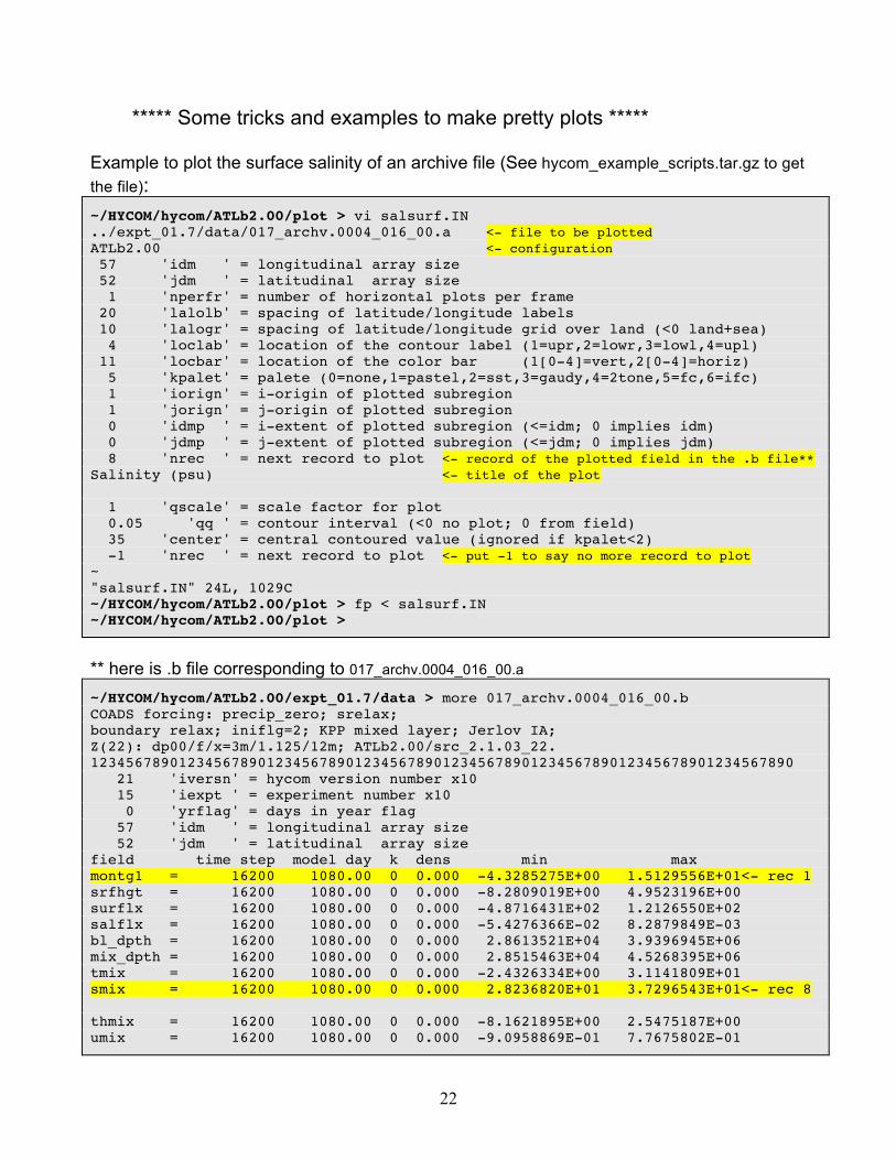
***** Some tricks and examples to make pretty plots ***** Example to plot the surface salinity of an archive file (See hycom_example_scripts.tar.gz to get the file): ~/HYCOM/hycom/ATLb2.00/plot > vi salsurf.IN ../expt_01.7/data/017_archv.0004_016_00.a <- file to be plotted ATLb2.00 <- configuration 57 'idm ' = longitudinal array size 52 'jdm ' = latitudinal array size 1 'nperfr' = number of horizontal plots per frame 20 'lalolb' = spacing of latitude/longitude labels 10 'lalogr' = spacing of latitude/longitude grid over land (<0 land+sea) 4 'loclab' = location of the contour label (1=upr,2=lowr,3=lowl,4=upl) 11 'locbar' = location of the color bar (1[0-4]=vert,2[0-4]=horiz) 5 'kpalet' = palete (0=none,1=pastel,2=sst,3=gaudy,4=2tone,5=fc,6=ifc) 1 'iorign' = i-origin of plotted subregion 1 'jorign' = j-origin of plotted subregion 0 'idmp ' = i-extent of plotted subregion (<=idm; 0 implies idm) 0 'jdmp ' = j-extent of plotted subregion (<=jdm; 0 implies jdm) 8 'nrec ' = next record to plot <- record of the plotted field in the .b file** Salinity (psu) <- title of the plot 1 'qscale' = scale factor for plot 0.05 'qq ' = contour interval (<0 no plot; 0 from field) 35 'center' = central contoured value (ignored if kpalet<2) -1 'nrec ' = next record to plot <- put -1 to say no more record to plot ~ "salsurf.IN" 24L, 1029C ~/HYCOM/hycom/ATLb2.00/plot > fp < salsurf.IN ~/HYCOM/hycom/ATLb2.00/plot >

** here is .b file corresponding to 017_archv.0004_016_00.a ~/HYCOM/hycom/ATLb2.00/expt_01.7/data > more 017_archv.0004_016_00.b COADS forcing: precip_zero; srelax; boundary relax; iniflg=2; KPP mixed layer; Jerlov IA; Z(22): dp00/f/x=3m/1.125/12m; ATLb2.00/src_2.1.03_22. 12345678901234567890123456789012345678901234567890123456789012345678901234567890 21 'iversn' = hycom version number x10 15 'iexpt ' = experiment number x10 0 'yrflag' = days in year flag 57 'idm ' = longitudinal array size 52 'jdm ' = latitudinal array size field time step model day k dens min max montg1 = 16200 1080.00 0 0.000 -4.3285275E+00 1.5129556E+01<- rec 1 srfhgt = 16200 1080.00 0 0.000 -8.2809019E+00 4.9523196E+00 surflx = 16200 1080.00 0 0.000 -4.8716431E+02 1.2126550E+02 salflx = 16200 1080.00 0 0.000 -5.4276366E-02 8.2879849E-03 bl_dpth = 16200 1080.00 0 0.000 2.8613521E+04 3.9396945E+06 mix_dpth = 16200 1080.00 0 0.000 2.8515463E+04 4.5268395E+06 tmix = 16200 1080.00 0 0.000 -2.4326334E+00 3.1141809E+01 smix = 16200 1080.00 0 0.000 2.8236820E+01 3.7296543E+01<- rec 8 thmix = 16200 1080.00 0 0.000 -8.1621895E+00 2.5475187E+00 umix = 16200 1080.00 0 0.000 -9.0958869E-01 7.7675802E-01

23

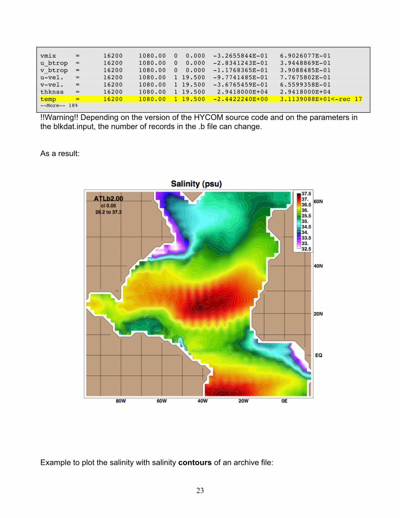
vmix = 16200 1080.00 0 0.000 -3.2655844E-01 6.9026077E-01 u_btrop = 16200 1080.00 0 0.000 -2.8341243E-01 3.9448869E-01 v_btrop = 16200 1080.00 0 0.000 -1.1768365E-01 3.9088485E-01 u-vel. = 16200 1080.00 1 19.500 -9.7741485E-01 7.7675802E-01 v-vel. = 16200 1080.00 1 19.500 -3.6765459E-01 6.5599358E-01 thknss = 16200 1080.00 1 19.500 2.9418000E+04 2.9418000E+04 temp = 16200 1080.00 1 19.500 -2.4422240E+00 3.1139088E+01<-rec 17 --More-- 18%

!!Warning!! Depending on the version of the HYCOM source code and on the parameters in the blkdat.input, the number of records in the .b file can change.

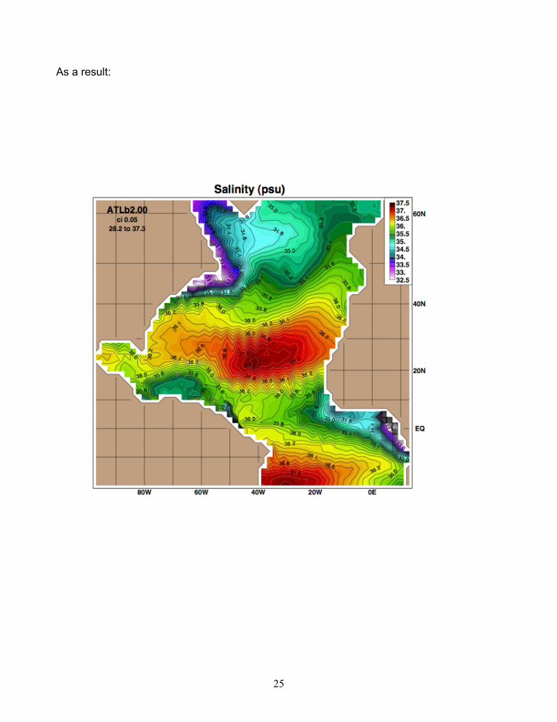
As a result:

Example to plot the salinity with salinity contours of an archive file:

24

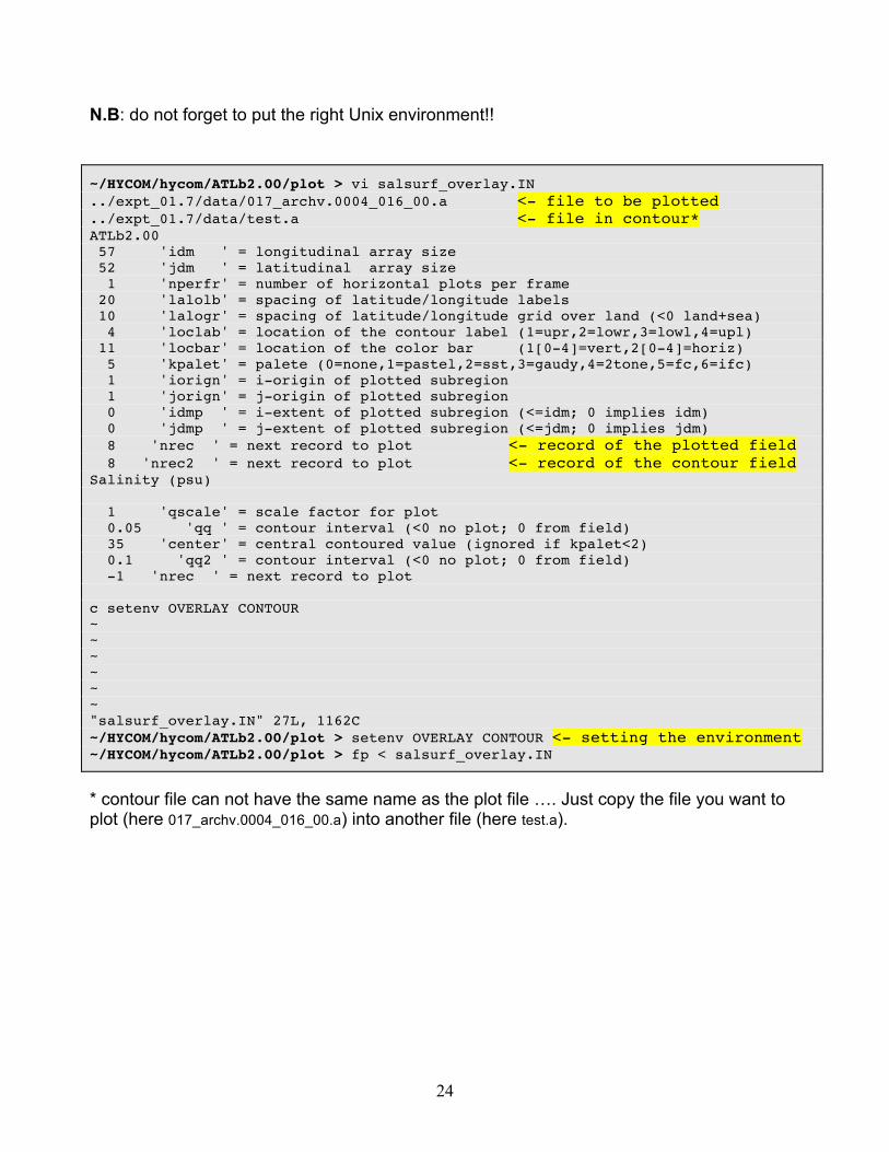
N.B: do not forget to put the right Unix environment!! ~/HYCOM/hycom/ATLb2.00/plot > vi salsurf_overlay.IN ../expt_01.7/data/017_archv.0004_016_00.a <- file to be plotted ../expt_01.7/data/test.a <- file in contour* ATLb2.00 57 'idm ' = longitudinal array size 52 'jdm ' = latitudinal array size 1 'nperfr' = number of horizontal plots per frame 20 'lalolb' = spacing of latitude/longitude labels 10 'lalogr' = spacing of latitude/longitude grid over land (<0 land+sea) 4 'loclab' = location of the contour label (1=upr,2=lowr,3=lowl,4=upl) 11 'locbar' = location of the color bar (1[0-4]=vert,2[0-4]=horiz) 5 'kpalet' = palete (0=none,1=pastel,2=sst,3=gaudy,4=2tone,5=fc,6=ifc) 1 'iorign' = i-origin of plotted subregion 1 'jorign' = j-origin of plotted subregion 0 'idmp ' = i-extent of plotted subregion (<=idm; 0 implies idm) 0 'jdmp ' = j-extent of plotted subregion (<=jdm; 0 implies jdm) 8 'nrec ' = next record to plot <- record of the plotted field 8 'nrec2 ' = next record to plot <- record of the contour field Salinity (psu) 1 'qscale' = scale factor for plot 0.05 'qq ' = contour interval (<0 no plot; 0 from field) 35 'center' = central contoured value (ignored if kpalet<2) 0.1 'qq2 ' = contour interval (<0 no plot; 0 from field) -1 'nrec ' = next record to plot c setenv OVERLAY CONTOUR ~ ~ ~ ~ ~ ~ "salsurf_overlay.IN" 27L, 1162C ~/HYCOM/hycom/ATLb2.00/plot > setenv OVERLAY CONTOUR <- setting the environment ~/HYCOM/hycom/ATLb2.00/plot > fp < salsurf_overlay.IN

* contour file can not have the same name as the plot file …. Just copy the file you want to plot (here 017_archv.0004_016_00.a) into another file (here test.a).

25

As a result:

26

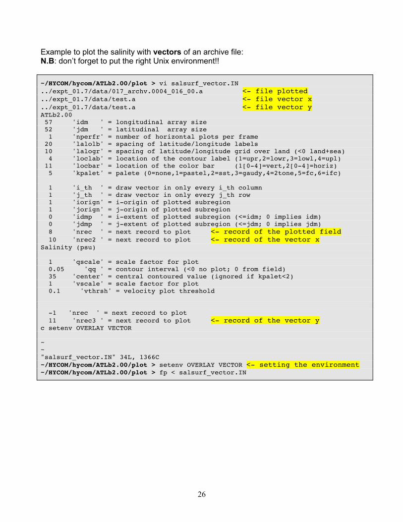
Example to plot the salinity with vectors of an archive file: N.B: don’t forget to put the right Unix environment!! ~/HYCOM/hycom/ATLb2.00/plot > vi salsurf_vector.IN ../expt_01.7/data/017_archv.0004_016_00.a <- file plotted ../expt_01.7/data/test.a <- file vector x ../expt_01.7/data/test.a <- file vector y ATLb2.00 57 'idm ' = longitudinal array size 52 'jdm ' = latitudinal array size 1 'nperfr' = number of horizontal plots per frame 20 'lalolb' = spacing of latitude/longitude labels 10 'lalogr' = spacing of latitude/longitude grid over land (<0 land+sea) 4 'loclab' = location of the contour label (1=upr,2=lowr,3=lowl,4=upl) 11 'locbar' = location of the color bar (1[0-4]=vert,2[0-4]=horiz) 5 'kpalet' = palete (0=none,1=pastel,2=sst,3=gaudy,4=2tone,5=fc,6=ifc) 1 'i_th ' = draw vector in only every i_th column 1 'j_th ' = draw vector in only every j_th row 1 'iorign' = i-origin of plotted subregion 1 'jorign' = j-origin of plotted subregion 0 'idmp ' = i-extent of plotted subregion (<=idm; 0 implies idm) 0 'jdmp ' = j-extent of plotted subregion (<=jdm; 0 implies jdm) 8 'nrec ' = next record to plot <- record of the plotted field 10 'nrec2 ' = next record to plot <- record of the vector x Salinity (psu) 1 'qscale' = scale factor for plot 0.05 'qq ' = contour interval (<0 no plot; 0 from field) 35 'center' = central contoured value (ignored if kpalet<2) 1 'vscale' = scale factor for plot 0.1 'vthrsh' = velocity plot threshold -1 'nrec ' = next record to plot 11 'nrec3 ' = next record to plot <- record of the vector y c setenv OVERLAY VECTOR ~ ~ "salsurf_vector.IN" 34L, 1366C ~/HYCOM/hycom/ATLb2.00/plot > setenv OVERLAY VECTOR <- setting the environment ~/HYCOM/hycom/ATLb2.00/plot > fp < salsurf_vector.IN

27

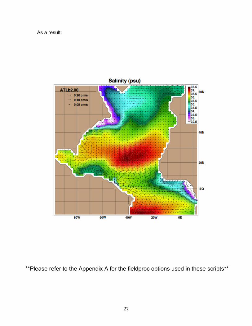
As a result:

**Please refer to the Appendix A for the fieldproc options used in these scripts**

28

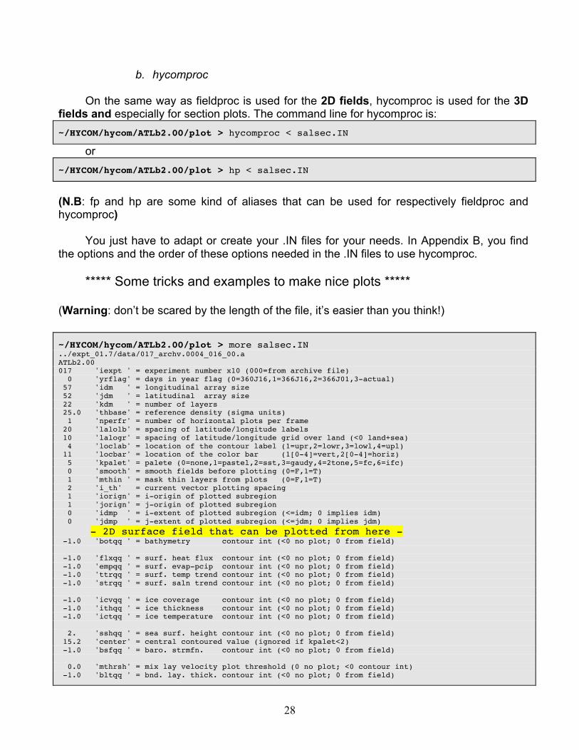
b. hycomproc

On the same way as fieldproc is used for the 2D fields, hycomproc is used for the 3D fields and especially for section plots. The command line for hycomproc is: ~/HYCOM/hycom/ATLb2.00/plot > hycomproc < salsec.IN

or ~/HYCOM/hycom/ATLb2.00/plot > hp < salsec.IN

(N.B: fp and hp are some kind of aliases that can be used for respectively fieldproc and hycomproc)

You just have to adapt or create your .IN files for your needs. In Appendix B, you find the options and the order of these options needed in the .IN files to use hycomproc.

***** Some tricks and examples to make nice plots ***** (Warning: don’t be scared by the length of the file, it’s easier than you think!) ~/HYCOM/hycom/ATLb2.00/plot > more salsec.IN ../expt_01.7/data/017_archv.0004_016_00.a ATLb2.00 017 'iexpt ' = experiment number x10 (000=from archive file) 0 'yrflag' = days in year flag (0=360J16,1=366J16,2=366J01,3-actual) 57 'idm ' = longitudinal array size 52 'jdm ' = latitudinal array size 22 'kdm ' = number of layers 25.0 'thbase' = reference density (sigma units) 1 'nperfr' = number of horizontal plots per frame 20 'lalolb' = spacing of latitude/longitude labels 10 'lalogr' = spacing of latitude/longitude grid over land (<0 land+sea) 4 'loclab' = location of the contour label (1=upr,2=lowr,3=lowl,4=upl) 11 'locbar' = location of the color bar (1[0-4]=vert,2[0-4]=horiz) 5 'kpalet' = palete (0=none,1=pastel,2=sst,3=gaudy,4=2tone,5=fc,6=ifc) 0 'smooth' = smooth fields before plotting (0=F,1=T) 1 'mthin ' = mask thin layers from plots (0=F,1=T) 2 'i_th' = current vector plotting spacing 1 'iorign' = i-origin of plotted subregion 1 'jorign' = j-origin of plotted subregion 0 'idmp ' = i-extent of plotted subregion (<=idm; 0 implies idm) 0 'jdmp ' = j-extent of plotted subregion (<=jdm; 0 implies jdm) - 2D surface field that can be plotted from here - -1.0 'botqq ' = bathymetry contour int (<0 no plot; 0 from field) -1.0 'flxqq ' = surf. heat flux contour int (<0 no plot; 0 from field) -1.0 'empqq ' = surf. evap-pcip contour int (<0 no plot; 0 from field) -1.0 'ttrqq ' = surf. temp trend contour int (<0 no plot; 0 from field) -1.0 'strqq ' = surf. saln trend contour int (<0 no plot; 0 from field) -1.0 'icvqq ' = ice coverage contour int (<0 no plot; 0 from field) -1.0 'ithqq ' = ice thickness contour int (<0 no plot; 0 from field) -1.0 'ictqq ' = ice temperature contour int (<0 no plot; 0 from field) 2. 'sshqq ' = sea surf. height contour int (<0 no plot; 0 from field) 15.2 'center' = central contoured value (ignored if kpalet<2) -1.0 'bsfqq ' = baro. strmfn. contour int (<0 no plot; 0 from field) 0.0 'mthrsh' = mix lay velocity plot threshold (0 no plot; <0 contour int) -1.0 'bltqq ' = bnd. lay. thick. contour int (<0 no plot; 0 from field)

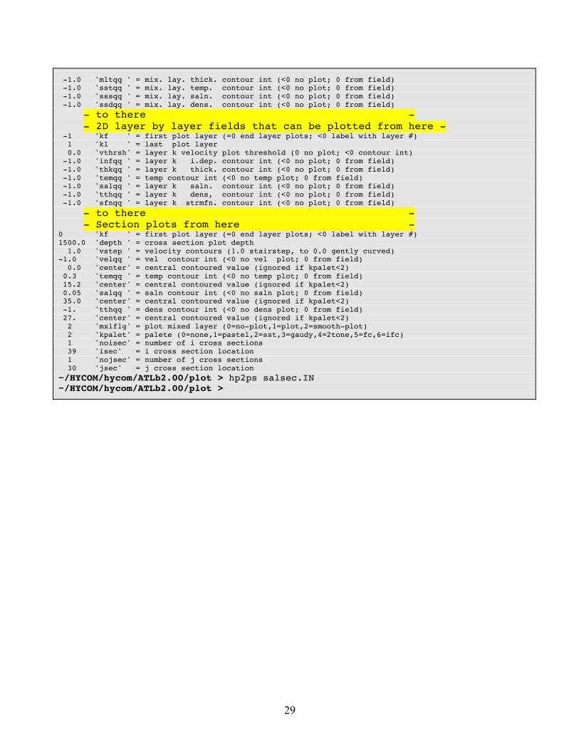
29

-1.0 'mltqq ' = mix. lay. thick. contour int (<0 no plot; 0 from field) -1.0 'sstqq ' = mix. lay. temp. contour int (<0 no plot; 0 from field) -1.0 'sssqq ' = mix. lay. saln. contour int (<0 no plot; 0 from field) -1.0 'ssdqq ' = mix. lay. dens. contour int (<0 no plot; 0 from field) - to there - - 2D layer by layer fields that can be plotted from here - -1 'kf ' = first plot layer (=0 end layer plots; <0 label with layer #) 1 'kl ' = last plot layer 0.0 'vthrsh' = layer k velocity plot threshold (0 no plot; <0 contour int) -1.0 'infqq ' = layer k i.dep. contour int (<0 no plot; 0 from field) -1.0 'thkqq ' = layer k thick. contour int (<0 no plot; 0 from field) -1.0 'temqq ' = temp contour int (<0 no temp plot; 0 from field) -1.0 'salqq ' = layer k saln. contour int (<0 no plot; 0 from field) -1.0 'tthqq ' = layer k dens, contour int (<0 no plot; 0 from field) -1.0 'sfnqq ' = layer k strmfn. contour int (<0 no plot; 0 from field) - to there - - Section plots from here - 0 'kf ' = first plot layer (=0 end layer plots; <0 label with layer #) 1500.0 'depth ' = cross section plot depth 1.0 'vstep ' = velocity contours (1.0 stairstep, to 0.0 gently curved) -1.0 'velqq ' = vel contour int (<0 no vel plot; 0 from field) 0.0 'center' = central contoured value (ignored if kpalet<2) 0.3 'temqq ' = temp contour int (<0 no temp plot; 0 from field) 15.2 'center' = central contoured value (ignored if kpalet<2) 0.05 'salqq ' = saln contour int (<0 no saln plot; 0 from field) 35.0 'center' = central contoured value (ignored if kpalet<2) -1. 'tthqq ' = dens contour int (<0 no dens plot; 0 from field) 27. 'center' = central contoured value (ignored if kpalet<2) 2 'mxlflg' = plot mixed layer (0=no-plot,1=plot,2=smooth-plot) 2 'kpalet' = palete (0=none,1=pastel,2=sst,3=gaudy,4=2tone,5=fc,6=ifc) 1 'noisec' = number of i cross sections 39 'isec' = i cross section location 1 'nojsec' = number of j cross sections 30 'jsec' = j cross section location ~/HYCOM/hycom/ATLb2.00/plot > hp2ps salsec.IN ~/HYCOM/hycom/ATLb2.00/plot >

30

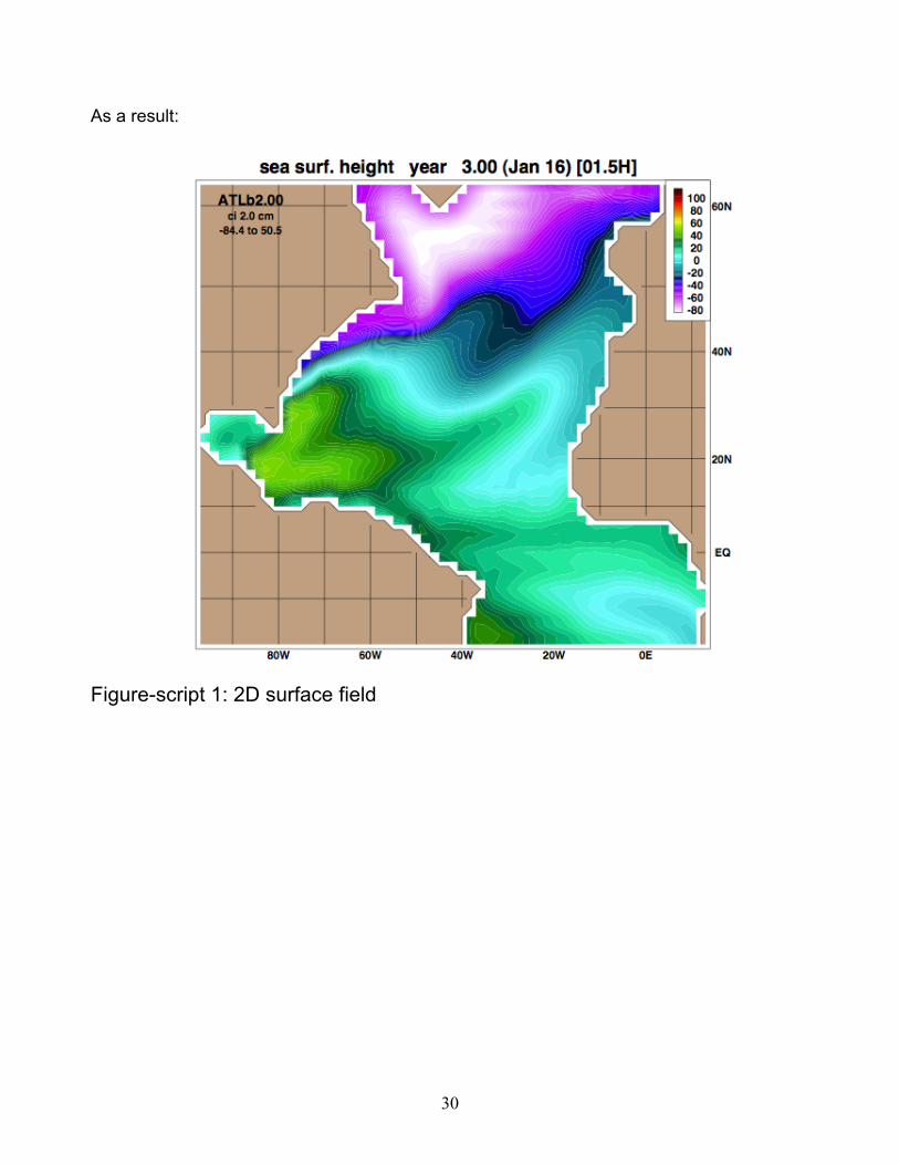
As a result:

Figure-script 1: 2D surface field

31

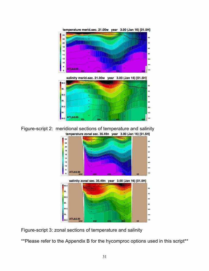
Figure-script 2: meridional sections of temperature and salinity

Figure-script 3: zonal sections of temperature and salinity **Please refer to the Appendix B for the hycomproc options used in this script**

32

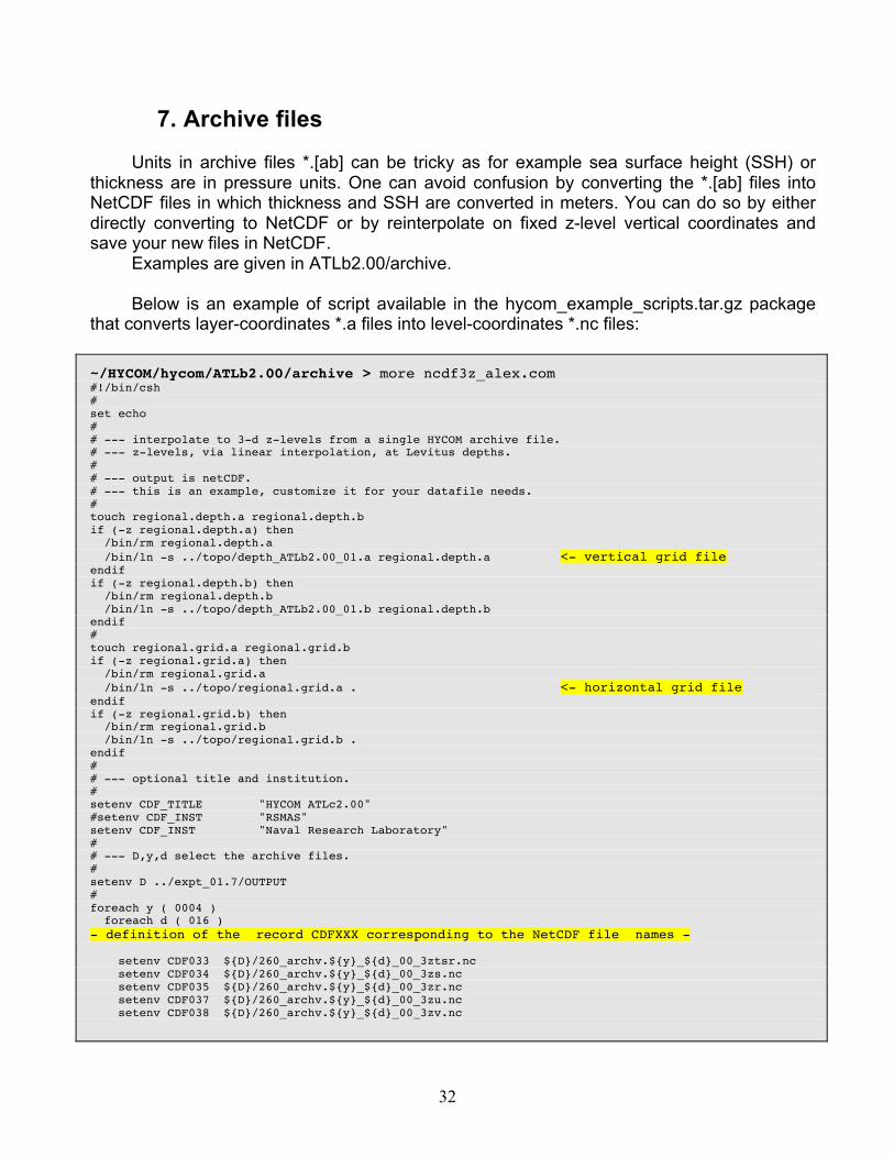
7. Archive files

Units in archive files *.[ab] can be tricky as for example sea surface height (SSH) or thickness are in pressure units. One can avoid confusion by converting the *.[ab] files into NetCDF files in which thickness and SSH are converted in meters. You can do so by either directly converting to NetCDF or by reinterpolate on fixed z-level vertical coordinates and save your new files in NetCDF.

Examples are given in ATLb2.00/archive. Below is an example of script available in the hycom_example_scripts.tar.gz package

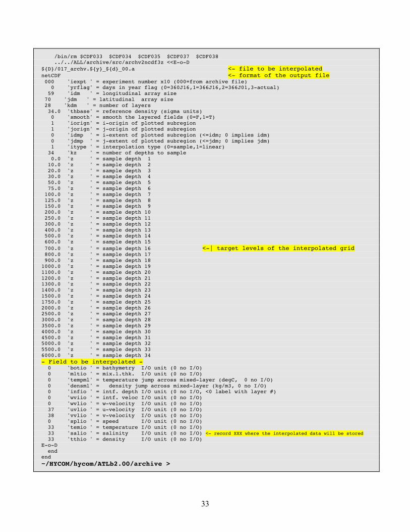
that converts layer-coordinates *.a files into level-coordinates *.nc files: ~/HYCOM/hycom/ATLb2.00/archive > more ncdf3z_alex.com #!/bin/csh # set echo # # --- interpolate to 3-d z-levels from a single HYCOM archive file. # --- z-levels, via linear interpolation, at Levitus depths. # # --- output is netCDF. # --- this is an example, customize it for your datafile needs. # touch regional.depth.a regional.depth.b if (-z regional.depth.a) then /bin/rm regional.depth.a /bin/ln -s ../topo/depth_ATLb2.00_01.a regional.depth.a <- vertical grid file endif if (-z regional.depth.b) then /bin/rm regional.depth.b /bin/ln -s ../topo/depth_ATLb2.00_01.b regional.depth.b endif # touch regional.grid.a regional.grid.b if (-z regional.grid.a) then /bin/rm regional.grid.a /bin/ln -s ../topo/regional.grid.a . <- horizontal grid file endif if (-z regional.grid.b) then /bin/rm regional.grid.b /bin/ln -s ../topo/regional.grid.b . endif # # --- optional title and institution. # setenv CDF_TITLE "HYCOM ATLc2.00" #setenv CDF_INST "RSMAS" setenv CDF_INST "Naval Research Laboratory" # # --- D,y,d select the archive files. # setenv D ../expt_01.7/OUTPUT # foreach y ( 0004 ) foreach d ( 016 ) - definition of the record CDFXXX corresponding to the NetCDF file names - setenv CDF033 ${D}/260_archv.${y}_${d}_00_3ztsr.nc setenv CDF034 ${D}/260_archv.${y}_${d}_00_3zs.nc setenv CDF035 ${D}/260_archv.${y}_${d}_00_3zr.nc setenv CDF037 ${D}/260_archv.${y}_${d}_00_3zu.nc setenv CDF038 ${D}/260_archv.${y}_${d}_00_3zv.nc

33

/bin/rm $CDF033 $CDF034 $CDF035 $CDF037 $CDF038 ../../ALL/archive/src/archv2ncdf3z <<E-o-D ${D}/017_archv.${y}_${d}_00.a <- file to be interpolated netCDF <- format of the output file 000 'iexpt ' = experiment number x10 (000=from archive file) 0 'yrflag' = days in year flag (0=360J16,1=366J16,2=366J01,3-actual) 59 'idm ' = longitudinal array size 70 'jdm ' = latitudinal array size 28 'kdm ' = number of layers 34.0 'thbase' = reference density (sigma units) 0 'smooth' = smooth the layered fields (0=F,1=T) 1 'iorign' = i-origin of plotted subregion 1 'jorign' = j-origin of plotted subregion 0 'idmp ' = i-extent of plotted subregion (<=idm; 0 implies idm) 0 'jdmp ' = j-extent of plotted subregion (<=jdm; 0 implies jdm) 1 'itype ' = interpolation type (0=sample,1=linear) 34 'kz ' = number of depths to sample 0.0 'z ' = sample depth 1 10.0 'z ' = sample depth 2 20.0 'z ' = sample depth 3 30.0 'z ' = sample depth 4 50.0 'z ' = sample depth 5 75.0 'z ' = sample depth 6 100.0 'z ' = sample depth 7 125.0 'z ' = sample depth 8 150.0 'z ' = sample depth 9 200.0 'z ' = sample depth 10 250.0 'z ' = sample depth 11 300.0 'z ' = sample depth 12 400.0 'z ' = sample depth 13 500.0 'z ' = sample depth 14 600.0 'z ' = sample depth 15 700.0 'z ' = sample depth 16 <-| target levels of the interpolated grid 800.0 'z ' = sample depth 17 900.0 'z ' = sample depth 18 1000.0 'z ' = sample depth 19 1100.0 'z ' = sample depth 20 1200.0 'z ' = sample depth 21 1300.0 'z ' = sample depth 22 1400.0 'z ' = sample depth 23 1500.0 'z ' = sample depth 24 1750.0 'z ' = sample depth 25 2000.0 'z ' = sample depth 26 2500.0 'z ' = sample depth 27 3000.0 'z ' = sample depth 28 3500.0 'z ' = sample depth 29 4000.0 'z ' = sample depth 30 4500.0 'z ' = sample depth 31 5000.0 'z ' = sample depth 32 5500.0 'z ' = sample depth 33 6000.0 'z ' = sample depth 34 - Field to be interpolated - 0 'botio ' = bathymetry I/O unit (0 no I/O) 0 'mltio ' = mix.l.thk. I/O unit (0 no I/O) 0 'tempml' = temperature jump across mixed-layer (degC, 0 no I/O) 0 'densml' = density jump across mixed-layer (kg/m3, 0 no I/O) 0 'infio ' = intf. depth I/O unit (0 no I/O, <0 label with layer #) 0 'wviio ' = intf. veloc I/O unit (0 no I/O) 0 'wvlio ' = w-velocity I/O unit (0 no I/O) 37 'uvlio ' = u-velocity I/O unit (0 no I/O) 38 'vvlio ' = v-velocity I/O unit (0 no I/O) 0 'splio ' = speed I/O unit (0 no I/O) 33 'temio ' = temperature I/O unit (0 no I/O) 33 'salio ' = salinity I/O unit (0 no I/O) <- record XXX where the interpolated data will be stored 33 'tthio ' = density I/O unit (0 no I/O) E-o-D end end ~/HYCOM/hycom/ATLb2.00/archive >

34

Now you are ready to use the HYCOM ocean model! Hope you have enjoyed the trip!

Do not hesitate to communicate some comments, corrections or contribution to this Quick start’s guide!

THE END

35

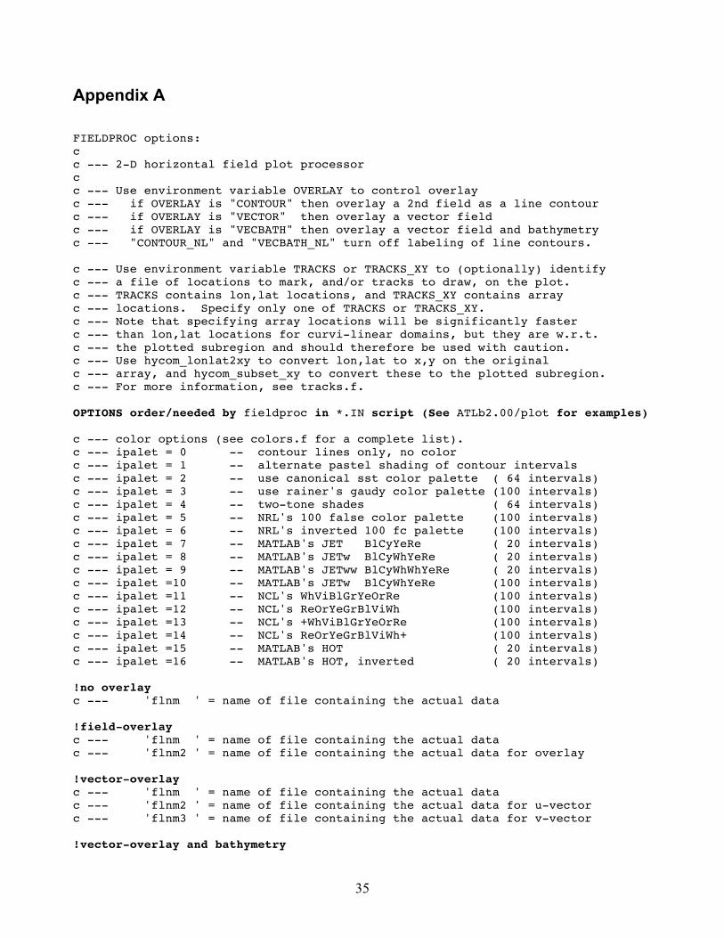
Appendix A FIELDPROC options: c c --- 2-D horizontal field plot processor c c --- Use environment variable OVERLAY to control overlay c --- if OVERLAY is "CONTOUR" then overlay a 2nd field as a line contour c --- if OVERLAY is "VECTOR" then overlay a vector field c --- if OVERLAY is "VECBATH" then overlay a vector field and bathymetry c --- "CONTOUR_NL" and "VECBATH_NL" turn off labeling of line contours. c --- Use environment variable TRACKS or TRACKS_XY to (optionally) identify c --- a file of locations to mark, and/or tracks to draw, on the plot. c --- TRACKS contains lon,lat locations, and TRACKS_XY contains array c --- locations. Specify only one of TRACKS or TRACKS_XY. c --- Note that specifying array locations will be significantly faster c --- than lon,lat locations for curvi-linear domains, but they are w.r.t. c --- the plotted subregion and should therefore be used with caution. c --- Use hycom_lonlat2xy to convert lon,lat to x,y on the original c --- array, and hycom_subset_xy to convert these to the plotted subregion. c --- For more information, see tracks.f. OPTIONS order/needed by fieldproc in *.IN script (See ATLb2.00/plot for examples) c --- color options (see colors.f for a complete list). c --- ipalet = 0 -- contour lines only, no color c --- ipalet = 1 -- alternate pastel shading of contour intervals c --- ipalet = 2 -- use canonical sst color palette ( 64 intervals) c --- ipalet = 3 -- use rainer's gaudy color palette (100 intervals) c --- ipalet = 4 -- two-tone shades ( 64 intervals) c --- ipalet = 5 -- NRL's 100 false color palette (100 intervals) c --- ipalet = 6 -- NRL's inverted 100 fc palette (100 intervals) c --- ipalet = 7 -- MATLAB's JET BlCyYeRe ( 20 intervals) c --- ipalet = 8 -- MATLAB's JETw BlCyWhYeRe ( 20 intervals) c --- ipalet = 9 -- MATLAB's JETww BlCyWhWhYeRe ( 20 intervals) c --- ipalet =10 -- MATLAB's JETw BlCyWhYeRe (100 intervals) c --- ipalet =11 -- NCL's WhViBlGrYeOrRe (100 intervals) c --- ipalet =12 -- NCL's ReOrYeGrBlViWh (100 intervals) c --- ipalet =13 -- NCL's +WhViBlGrYeOrRe (100 intervals) c --- ipalet =14 -- NCL's ReOrYeGrBlViWh+ (100 intervals) c --- ipalet =15 -- MATLAB's HOT ( 20 intervals) c --- ipalet =16 -- MATLAB's HOT, inverted ( 20 intervals) !no overlay c --- 'flnm ' = name of file containing the actual data !field-overlay c --- 'flnm ' = name of file containing the actual data c --- 'flnm2 ' = name of file containing the actual data for overlay !vector-overlay c --- 'flnm ' = name of file containing the actual data c --- 'flnm2 ' = name of file containing the actual data for u-vector c --- 'flnm3 ' = name of file containing the actual data for v-vector !vector-overlay and bathymetry

36

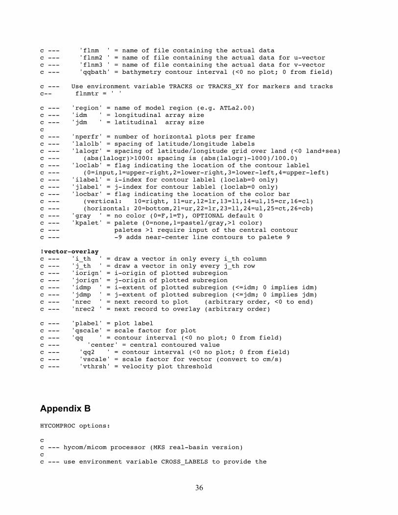
c --- 'flnm ' = name of file containing the actual data c --- 'flnm2 ' = name of file containing the actual data for u-vector c --- 'flnm3 ' = name of file containing the actual data for v-vector c --- 'qqbath' = bathymetry contour interval (<0 no plot; 0 from field) c --- Use environment variable TRACKS or TRACKS_XY for markers and tracks c-- flnmtr = ' ' c --- 'region' = name of model region (e.g. ATLa2.00) c --- 'idm ' = longitudinal array size c --- 'jdm ' = latitudinal array size c c --- 'nperfr' = number of horizontal plots per frame c --- 'lalolb' = spacing of latitude/longitude labels c --- 'lalogr' = spacing of latitude/longitude grid over land (<0 land+sea) c --- (abs(lalogr)>1000: spacing is (abs(lalogr)-1000)/100.0) c --- 'loclab' = flag indicating the location of the contour lablel c --- (0=input,1=upper-right,2=lower-right,3=lower-left,4=upper-left) c --- 'ilabel' = i-index for contour lablel (loclab=0 only) c --- 'jlabel' = j-index for contour lablel (loclab=0 only) c --- 'locbar' = flag indicating the location of the color bar c --- (vertical: 10=right, 11=ur,12=lr,13=ll,14=ul,15=cr,16=cl) c --- (horizontal: 20=bottom,21=ur,22=lr,23=ll,24=ul,25=ct,26=cb) c --- 'gray ' = no color (0=F,1=T), OPTIONAL default 0 c --- 'kpalet' = palete (0=none,1=pastel/gray,>1 color) c --- paletes >1 require input of the central contour c --- -9 adds near-center line contours to palete 9

!vector-overlay c --- 'i_th ' = draw a vector in only every i_th column c --- 'j_th ' = draw a vector in only every j_th row c --- 'iorign' = i-origin of plotted subregion c --- 'jorign' = j-origin of plotted subregion c --- 'idmp ' = i-extent of plotted subregion (<=idm; 0 implies idm) c --- 'jdmp ' = j-extent of plotted subregion (<=jdm; 0 implies jdm) c --- 'nrec ' = next record to plot (arbitrary order, <0 to end) c --- 'nrec2 ' = next record to overlay (arbitrary order) c --- 'plabel' = plot label c --- 'qscale' = scale factor for plot c --- 'qq ' = contour interval (<0 no plot; 0 from field) c --- 'center' = central contoured value c --- 'qq2 ' = contour interval (<0 no plot; 0 from field) c --- 'vscale' = scale factor for vector (convert to cm/s) c --- 'vthrsh' = velocity plot threshold

Appendix B HYCOMPROC options: c c --- hycom/micom processor (MKS real-basin version) c c --- use environment variable CROSS_LABELS to provide the

37

c --- name of a file containing a 4-character label for each c --- layer on cross-section plots. Note that CROSS_LABELS="NONE" c --- indicates no cross section plots are needed (i.e. no[ij]sec=0), c --- and can speed up the processing in such cases. c c --- Use environment variable TRACKS or TRACKS_XY to (optionally) identify c --- a file of locations to mark, and/or tracks to draw, on the lon-lat plot. c --- TRACKS contains lon,lat locations, and TRACKS_XY contains array c --- locations. Specify only one of TRACKS or TRACKS_XY. c --- Note that specifying array locations will be significantly faster c --- than lon,lat locations for curvi-linear domains, but they are w.r.t. c --- the plotted subregion and should therefore be used with caution. c --- Use hycom_lonlat2xy to convert lon,lat to x,y on the original c --- array, and hycom_subset_xy to convert these to the plotted subregion. c --- For more information, see tracks.f. OPTIONS order/needed by hycomproc in *.IN script (See ATL/plot for examples) c --- color options (see colors.f for a complete list). c --- ipalet = 0 -- contour lines only, no color c --- ipalet = 1 -- alternate pastel shading or negative gray c --- ipalet = 2 -- use canonical sst color palette ( 64 intervals) c --- ipalet = 3 -- use rainer's gaudy color palette (100 intervals) c --- ipalet = 4 -- two-tone shades ( 64 intervals) c --- ipalet = 5 -- NRL's 100 false color palette (100 intervals) c --- ipalet = 6 -- NRL's inverted 100 fc palette (100 intervals) c --- ipalet = 7 -- MATLAB's JET BlCyYeRe ( 20 intervals) c --- ipalet = 8 -- MATLAB's JETw BlCyWhYeRe ( 20 intervals) c --- ipalet = 9 -- MATLAB's JETww BlCyWhWhYeRe ( 20 intervals) c --- ipalet =10 -- MATLAB's JETw BlCyWhYeRe (100 intervals) c --- ipalet =11 -- NCL's WhViBlGrYeOrRe (100 intervals) c --- ipalet =12 -- NCL's ReOrYeGrBlViWh (100 intervals) c --- ipalet =13 -- NCL's +WhViBlGrYeOrRe (100 intervals) c --- ipalet =14 -- NCL's ReOrYeGrBlViWh+ (100 intervals) c --- ipalet =15 -- MATLAB's HOT ( 20 intervals) c --- ipalet =16 -- MATLAB's HOT, inverted ( 20 intervals) c c c --- 'region' = name of model region (e.g. ATLa2.00) c --- 'iexpt ' = experiment number x10 (000=from archive file) c --- 'yrflag' = days in year flag (-1=none,0=360,1=366J16,2=366J01,3=actual) c --- 'ntracr' = number of tracers (to plot, optional with default 0) c --- one line per tracer: 8-letter title, 8-letter format, long name c --- 'idm ' = longitudinal array size c --- 'jdm ' = latitudinal array size c --- 'kdm ' = number of layers c c --- 'thbase' = reference density (sigma units) c --- 'nperfr' = number of horizontal plots per frame c --- 'lalolb' = spacing of latitude/longitude labels (<0 use array spacing) c --- 'lalogr' = spacing of latitude/longitude grid over land (<0 land+sea) c --- (abs(lalogr)>1000: spacing is (abs(lalogr)-1000)/100.0) c --- 'loclab' = flag indicating the location of the contour lablel c --- (0=input,1=upper-right,2=lower-right,3=lower-left,4=upper-left) c --- 'ilabel' = i-index for contour lablel (loclab=0 only)

38

c --- 'jlabel' = j-index for contour lablel (loclab=0 only) c --- 'locbar' = flag indicating the location of the color bar c --- (vertical: 10=right, 11=ur,12=lr,13=ll,14=ul,15=cr,16=cl) c --- (horizontal: 20=bottom,21=ur,22=lr,23=ll,24=ul,25=ct,26=cb) c --- 'gray ' = no color (0=F,1=T), OPTIONAL default 0 c --- 'kpalet' = palete (0=none,1=pastel/gray,>1 color) c --- paletes >1 require input of the central contour c --- 'smooth' = smooth fields before plotting c --- 'mthin ' = mask thin layers from plots (0=F,1=T,2=T&mdens=T) c --- 'baclin' = plot baroclinic velocity (0=total:DEFAULT,1=baroclinic) c --- 'i_th ' = draw only every i_th vector in every (i_th/2) row c --- 'iorign' = i-origin of plotted subregion c --- 'jorign' = j-origin of plotted subregion c --- 'idmp ' = i-extent of plotted subregion (<=idm; 0 implies idm) c --- 'jdmp ' = j-extent of plotted subregion (<=jdm; 0 implies jdm) c --- ----------------------- c --- plot non-layered fields c --- ----------------------- c c --- 'botqq ' = bathymetry contour int (<0 no plot; 0 from field) c --- 'center' = central contoured value c c --- ------------------- c --- plot surface fluxes c --- ------------------- c c --- 'flxqq ' = surf. heat flux contour int (<0 no plot; 0 from field) c --- 'center' = central contoured value c --- 'empqq ' = surf. evap-pcip contour int (<0 no plot; 0 from field) c --- 'center' = central contoured value c --- 'ttrqq ' = surf. temp trend contour int (<0 no plot; 0 from field) c --- 'center' = central contoured value c --- 'strqq ' = surf. saln trend contour int (<0 no plot; 0 from field) c --- 'center' = central contoured value c c --- --------------- c --- plot ice fields c --- --------------- c * if (icegln) then c c --- 'icvqq ' = ice coverage contour int (<0 no plot; 0 from field) c --- 'center' = central contoured value c --- 'ithqq ' = ice thickness contour int (<0 no plot; 0 from field) c --- 'center' = central contoured value c --- 'ictqq ' = ice temperature contour int (<0 no plot; 0 from field) c --- 'center' = central contoured value c --- ------------------- c --- plot surface fields c --- -------------------

39

c c --- 'sshqq ' = sea surf. height contour int (<0 no plot; 0 from field) c --- 'center' = central contoured value c --- 'bkeqq ' = baro. kinetic energy contour int (<0 no plot; 0 from field) c --- 'center' = central contoured value c --- ------------------------ c --- plot barotropic velocity c --- ------------------------ c --- 'bspdqq' = barotropic speed contour interval (<0 no plot; 0 from field) c --- 'center' = central contoured value (if needed) c --- 'bthrsh' = barotropic velocity plot threshold (0 no plot; <0 contour int) c --- 'center' = central contoured value c --- also have 'vthrsh' and 'bsfqq ' c --- 'bsfqq ' = baro. strmfn. contour int (<0 no plot; 0 from field) c --- 'center' = central contoured value c c --- ----------------------- c --- plot mixed layer fields c --- ----------------------- c c --- 'mthrsh' = mix lay velocity plot threshold (0 no plot; <0 contour int) c --- 'bltqq ' = bnd. lay. thick. contour int (<0 no plot; 0 from field) c --- 'center' = central contoured value c --- 'mltqq ' = mix. lay. thick. contour int (<0 no plot; 0 from field) c --- 'center' = central contoured value c --- 'sstqq ' = mix. lay. temp. contour int (<0 no plot; 0 from field) c --- 'center' = central contoured value c --- 'sssqq ' = mix. lay. saln. contour int (<0 no plot; 0 from field) c --- 'center' = central contoured value c --- 'ssdqq ' = mix. lay. dens. contour int (<0 no plot; 0 from field) c --- 'center' = central contoured value c --- 'mkeqq ' = m.l. kinetic energy contour int (<0 no plot; 0 from field) c --- 'center' = central contoured value c c --- -------------------- c --- plot selected layers c --- -------------------- c c --- 'kf ' = first plot layer (=0 end layer plots; <0 label with layer #) c --- 'kl ' = last plot layer c c --- ------------------- c --- plot layer velocity c --- ------------------- c --- 'spdqq ' = layer k speed contour int (<0 no plot; 0 from field) c --- 'vthrsh' = layer k velocity plot threshold (0 no plot; <0 contour int) c --- 'center' = central contoured value c c --- ---------------------------- c --- plot fluid vertical velocity

40

c --- ---------------------------- c --- 'wvelqq' = lay. k w-vel. contour int (<0 no plot; 0 from field) c --- 'infqq ' = lay. k thick. contour int (<0 no plot; 0 from field) c --- 'center' = central contoured value c c --- -------------------- c --- plot interface depth c --- -------------------- c c --- 'infqq ' = lay. k thick. contour int (<0 no plot; 0 from field) c --- 'center' = central contoured value c c --- -------------------- c --- plot layer thickness c --- -------------------- c c --- 'thkqq ' = lay. k thick. contour int (<0 no plot; 0 from field) c --- 'center' = central contoured value c c --- ---------------- c --- plot temperature c --- ---------------- c c --- 'temqq ' = layer k temp contour int (<0 no plot; 0 from field) c --- 'center' = central contoured value c c --- ------------- c --- plot salinity c --- ------------- c c --- 'salqq ' = lay. k saln. contour int (<0 no plot; 0 from field) c --- 'center' = central contoured value c c --- ------------- c --- plot density c --- ------------- c c --- 'tthqq ' = layer k density contour int (<0 no plot; 0 from field) c --- 'center' = central contoured value c c --- ------------ c --- plot tracers c --- ------------ c c --- 'trcqq ' = layer k tracer contour int (<0 no plot; 0 from field) c --- 'center' = central contoured value c c --- -------------------------- c --- plot layer kinetic energy c --- -------------------------- c c --- 'keqq ' = kinetic energy contour int (<0 no plot; 0 from field) c --- 'center' = central contoured value c c --- --------------------------

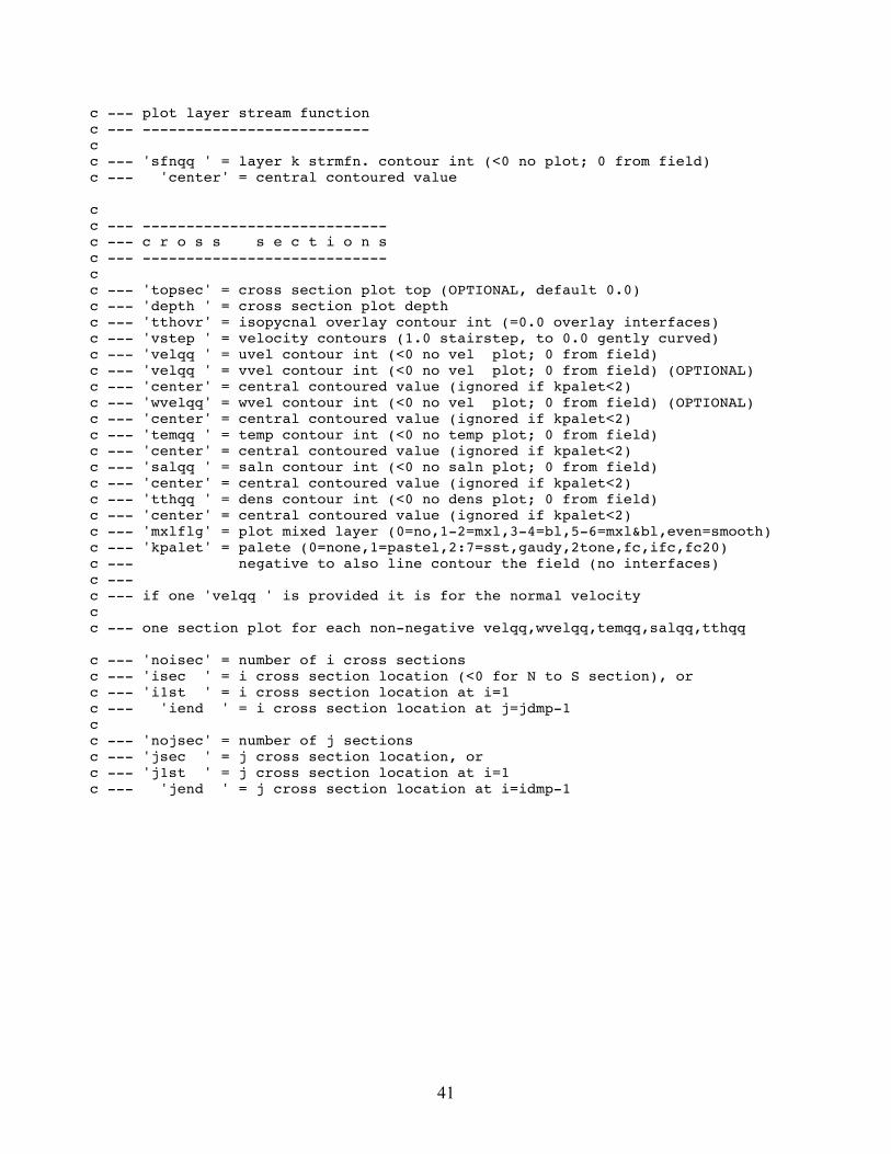
41

c --- plot layer stream function c --- -------------------------- c c --- 'sfnqq ' = layer k strmfn. contour int (<0 no plot; 0 from field) c --- 'center' = central contoured value c c --- ---------------------------- c --- c r o s s s e c t i o n s c --- ---------------------------- c c --- 'topsec' = cross section plot top (OPTIONAL, default 0.0) c --- 'depth ' = cross section plot depth c --- 'tthovr' = isopycnal overlay contour int (=0.0 overlay interfaces) c --- 'vstep ' = velocity contours (1.0 stairstep, to 0.0 gently curved) c --- 'velqq ' = uvel contour int (<0 no vel plot; 0 from field) c --- 'velqq ' = vvel contour int (<0 no vel plot; 0 from field) (OPTIONAL) c --- 'center' = central contoured value (ignored if kpalet<2) c --- 'wvelqq' = wvel contour int (<0 no vel plot; 0 from field) (OPTIONAL) c --- 'center' = central contoured value (ignored if kpalet<2) c --- 'temqq ' = temp contour int (<0 no temp plot; 0 from field) c --- 'center' = central contoured value (ignored if kpalet<2) c --- 'salqq ' = saln contour int (<0 no saln plot; 0 from field) c --- 'center' = central contoured value (ignored if kpalet<2) c --- 'tthqq ' = dens contour int (<0 no dens plot; 0 from field) c --- 'center' = central contoured value (ignored if kpalet<2) c --- 'mxlflg' = plot mixed layer (0=no,1-2=mxl,3-4=bl,5-6=mxl&bl,even=smooth) c --- 'kpalet' = palete (0=none,1=pastel,2:7=sst,gaudy,2tone,fc,ifc,fc20) c --- negative to also line contour the field (no interfaces) c --- c --- if one 'velqq ' is provided it is for the normal velocity c c --- one section plot for each non-negative velqq,wvelqq,temqq,salqq,tthqq c --- 'noisec' = number of i cross sections c --- 'isec ' = i cross section location (<0 for N to S section), or c --- 'i1st ' = i cross section location at i=1 c --- 'iend ' = i cross section location at j=jdmp-1 c c --- 'nojsec' = number of j sections c --- 'jsec ' = j cross section location, or c --- 'j1st ' = j cross section location at i=1 c --- 'jend ' = j cross section location at i=idmp-1