Hydrodynamic and sediment transport modelling in the canals of Venice (Italy)

Estuarine, Coastal and Shelf Science 75 (2007) 250e260www.elsevier.com/locate/ecss

Hydrodynamic and sediment transport modelling in thecanals of Venice (Italy)

Elisa Coraci, Georg Umgiesser*, Roberto Zonta

CNR-ISMAR, Consiglio Nazionale delle Ricerche, Istituto di Scienze Marine, San Polo, 1364, 30125 Venezia, Italy

Received 15 October 2006; accepted 8 February 2007

Available online 9 July 2007

Abstract

A framework of numerical models was applied to the canal network of Venice in order to simulate hydrodynamics and sediment transport. Atwo-dimensional finite element model (SHYFEM) was applied to the whole surrounding lagoon using water levels as a forcing. The computedlevels were extracted along the contour of the city of Venice and then a link-node model was run in the canal network. The simulated variableswere calibrated and compared with data from field measurements. Calculated water elevation displays a good agreement with the measured data,and current velocity is well reproduced. Simulations were initially carried out using a constant Manning parameter (MC) and successively a vary-ing coefficient (VMC) was adopted, in order to account for the different depths of the canals. By applying the sediment transport module anevaluation of the sediment accumulation rate in the canal network was obtained, permitting an estimation of the yearly silting up of the canalbed. Different simulations were carried out considering material input from both the city and the lagoon. The model is able to reproduce theoverall accretion rate of the canal bottom, and it is a useful tool for planning the dredging activities in the whole canal network.� 2007 Elsevier Ltd. All rights reserved.

Keywords: Venice Lagoon; Venice canals; numerical modelling; sediment transport; silting

1. Introduction

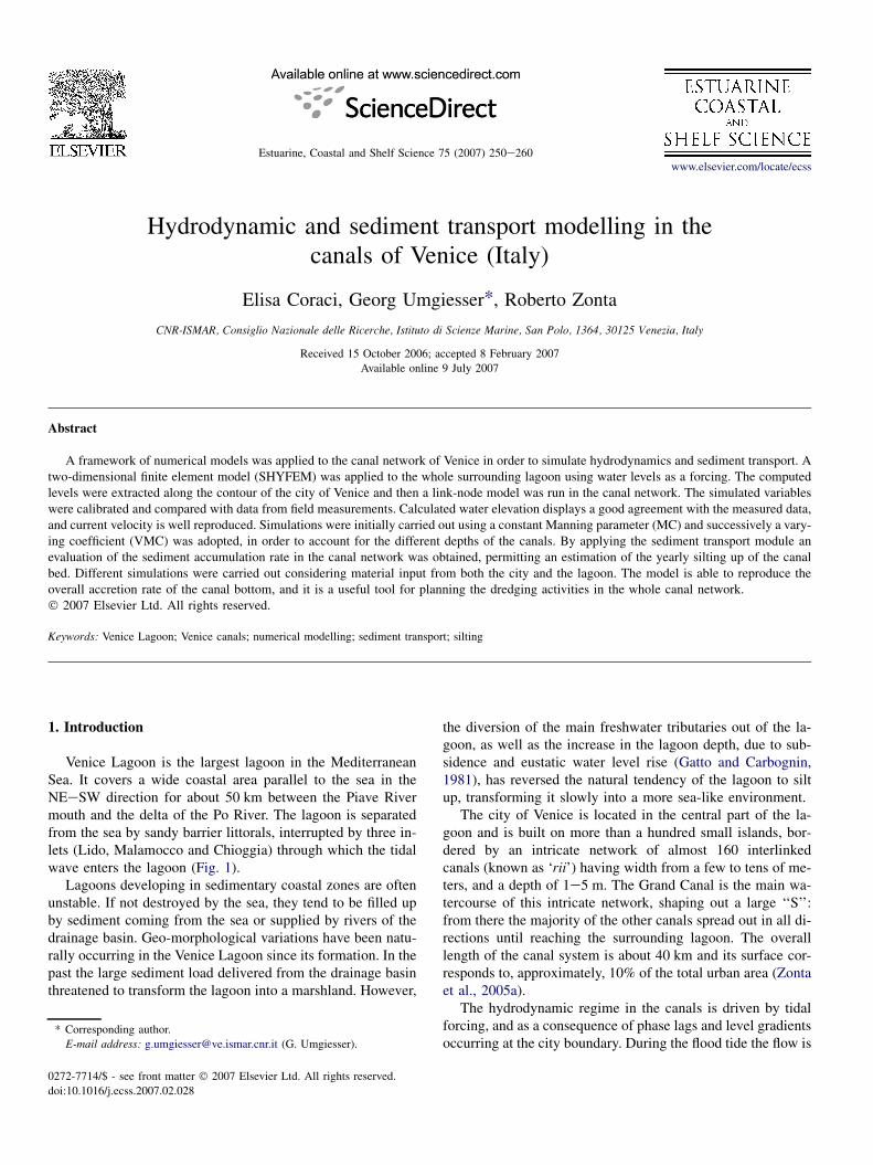
Venice Lagoon is the largest lagoon in the MediterraneanSea. It covers a wide coastal area parallel to the sea in theNEeSW direction for about 50 km between the Piave Rivermouth and the delta of the Po River. The lagoon is separatedfrom the sea by sandy barrier littorals, interrupted by three in-lets (Lido, Malamocco and Chioggia) through which the tidalwave enters the lagoon (Fig. 1).

Lagoons developing in sedimentary coastal zones are oftenunstable. If not destroyed by the sea, they tend to be filled upby sediment coming from the sea or supplied by rivers of thedrainage basin. Geo-morphological variations have been natu-rally occurring in the Venice Lagoon since its formation. In thepast the large sediment load delivered from the drainage basinthreatened to transform the lagoon into a marshland. However,

* Corresponding author.

E-mail address: [email protected] (G. Umgiesser).

0272-7714/$ - see front matter � 2007 Elsevier Ltd. All rights reserved.

doi:10.1016/j.ecss.2007.02.028

the diversion of the main freshwater tributaries out of the la-goon, as well as the increase in the lagoon depth, due to sub-sidence and eustatic water level rise (Gatto and Carbognin,1981), has reversed the natural tendency of the lagoon to siltup, transforming it slowly into a more sea-like environment.

The city of Venice is located in the central part of the la-goon and is built on more than a hundred small islands, bor-dered by an intricate network of almost 160 interlinkedcanals (known as ‘rii’) having width from a few to tens of me-ters, and a depth of 1e5 m. The Grand Canal is the main wa-tercourse of this intricate network, shaping out a large ‘‘S’’:from there the majority of the other canals spread out in all di-rections until reaching the surrounding lagoon. The overalllength of the canal system is about 40 km and its surface cor-responds to, approximately, 10% of the total urban area (Zontaet al., 2005a).

The hydrodynamic regime in the canals is driven by tidalforcing, and as a consequence of phase lags and level gradientsoccurring at the city boundary. During the flood tide the flow is

mailto:[email protected]

http://www.elsevier.com/locate/ecss

251E. Coraci et al. / Estuarine, Coastal and Shelf Science 75 (2007) 250e260

Fig. 1. The Venice Lagoon with the SHYFEM finite element grid.

predominantly from SE to NW, while the direction is reversedin the ebb. Current speed in the network is low, with averagemaximum values of up to 25 cm s�1 throughout the tidal cycle.

Besides constituting the principal way of transportation forhuman and public services, the canal network is the collectorof all types of urban refuse from untreated domestic and com-mercial sewage effluents. Venice, in fact, does not have a realsewage system. Due to the sluggish circulation, the deliveredorganic and inorganic matter, as well as materials erodedfrom the urban surfaces, reach the network, allowing for a pro-gressive silting up of the canal bottom.

After a long period (1960e1995) where no dredging oc-curred, the Municipality of Venice started an overall seriesof dredging activities to permit navigation and maintaina healthy environment. Today, a general improvement of thesewage system has commenced including septic tanks andsmall wastewater treatment plants, as well as the restorationof building foundations and consolidation of canal walls (Gar-din, 1999).

As a consequence, a reduction of the loading of particulate,organic matter and contaminants to the canal network is ex-pected to occur. Due to a growing interest towards the ecolog-ical problems of the canals, various research projectsregarding behaviour and quality of the network were per-formed in recent years (Collavini et al., 2004; Zonta et al.,2005b, 2006; D’Este et al., 2006).

Concerning hydrodynamics and modelling, De Marchi(1993) first applied a simple link-node model to the canal

network. Successively a new link-node one-dimensionalmodel (DYNHYD), that is the hydrodynamic module of thewater quality model WASP (Ambrose et al., 1993), was em-ployed and calibrated with field measurements (Zampato andUmgiesser, 2000; Umgiesser and Zampato, 2001). This canalmodel was coupled with a finite element model of the lagoon(SHYFEM). The further step was to modify the link-nodemodel from 1D to 2D structure in order to describe the sedimenttransport in the canal network (Umgiesser and Massalin, 2000).

This paper presents the results of the recent modelling ac-tivity carried out in the canal network, in the framework ofthe project QUEST (QUality, Efficiency, Sedimentation andTransport in the Venice canal network). The aforementioned2D canal model was improved creating a new link-node gridthat has a greater accuracy in reproducing the canal shape.A new data set (water level and speed) was acquired to cali-brate the model and to obtain a more complete investigationon the hydrodynamics of the canal system. Moreover, the sed-iment transport module was implemented in the erosion equa-tion and tested, allowing for a comparison with field dataderived from the bathymetric measurements. The sediment dy-namic was finally investigated to quantify the material flux toand from the canal bottom. A first attempt at estimating thecontribution of different sediment sources, both inside and out-side the city, was made in order to evaluate erosion and depo-sition rates in the canals. A further objective of this study wasto create a useful tool for planning the dredging activities inthe whole canal network.

252 E. Coraci et al. / Estuarine, Coastal and Shelf Science 75 (2007) 250e260

2. Methods

2.1. Field data

For the purpose of calibrating the model of the canal net-work, both hydrodynamic and sedimentological data wereneeded.

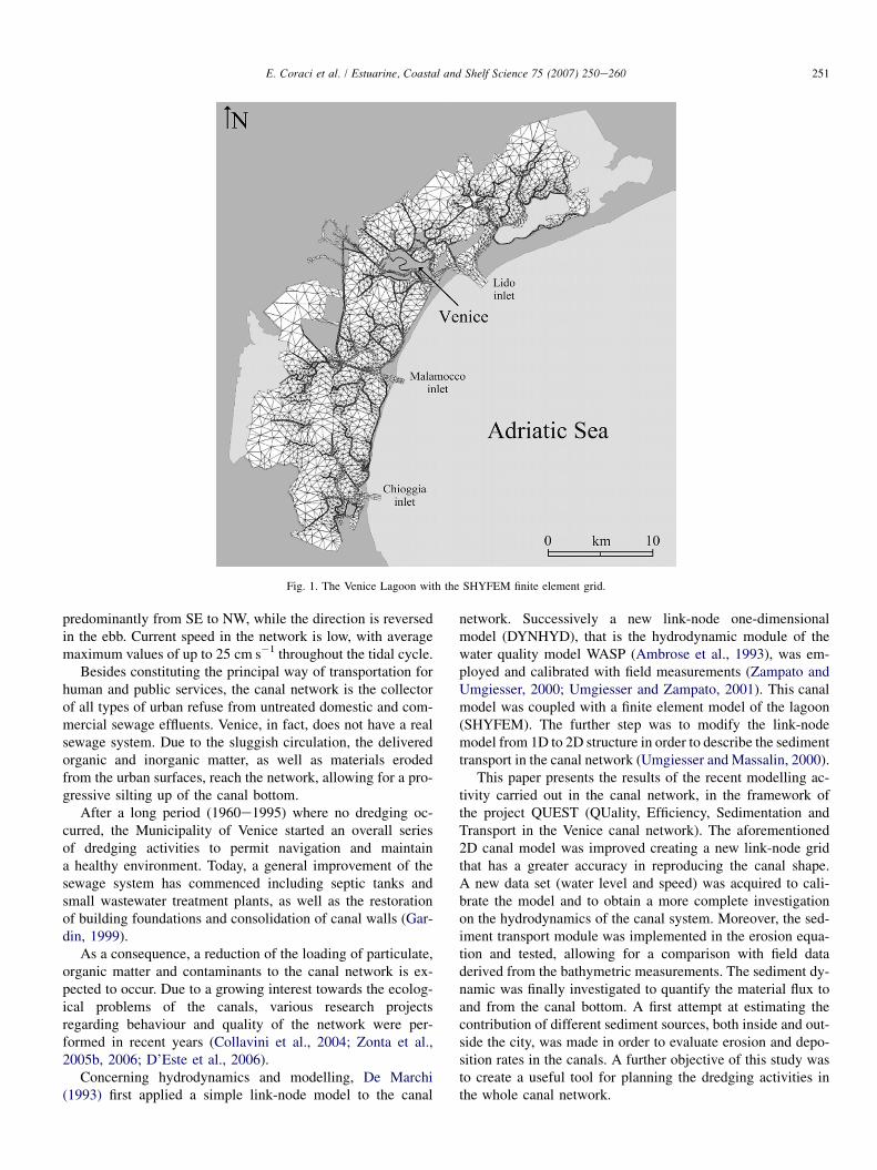
Time series of hydrodynamic data were acquired in the pe-riod from October to December 2004, in four zones of the city:San Polo, Santa Marta, Cannaregio, and Sant’Elena (Fig. 2).Three canals were chosen in every zone, and self-recordingelectromagnetic current meters (S4, InterOcean, USA) weredeployed for a time period of 15 days in each of the canalsto record water level and current speed. The sampling fre-quency of the data was 5 min. Data acquired were processedusing a 1-h moving average to smooth peaks generated bythe boat traffic.

To get a measured value of the canal bottom, the bathymet-ric data acquired by Insula (the company which is in charge ofthe interventions on the canal network) were used. The depthvariation was calculated from two field measurements carriedout in a time period which varied from two to five years. Theavailable data cover 50% of the canal network extent.

The mean value of sediment density, 1540 kg m�3, was de-rived from the available measured data regarding the sedimentcomposition in the canal network of Venice (Venice Munici-pality database).

2.2. The hydrodynamic models

The lagoon and the canal network are two environmentswith different morphological characteristics: the mean depthof the lagoon is about 1 m while the canal depth ranges aboutfrom 1 to 5 m; moreover, the canals have small width in com-parison with their length. As a consequence, two differenttypes of models were used.

2.2.1. The Venice Lagoon modelFor the lagoon, the 2D finite element shallow-water model

SHYFEM (Umgiesser and Bergamasco, 1993; Umgiesseret al., 2004) was used. The finite element method permits todescribe with a great detail the morphology and bathymetryof the area, and to represent with higher resolution the zoneswhere hydrodynamic features are more interesting. The nu-merical computation was carried out on a spatial domain thatrepresents the entire lagoon through a finite element grid(Fig. 1). The latter contains 4237 nodes and 7666 triangularelements. The model considers the three lagoon inlets as openboundaries, while the rest of the perimeter of the lagoon asa closed boundary.

The model resolves, with a semi-implicit time steppingscheme, the vertically integrated shallow-water equations intheir formulations with level and transports:

vU

vtþ gH

vh

vxþRUþX ¼ 0 ð1Þ

vV

vtþ gH

vh

vyþRV þ Y ¼ 0 ð2Þ

vh

vtþ vU

vxþ vV

vy¼ 0; ð3Þ

where h [m] is the water level, g is the gravitational accelera-tion [m s�2], H ¼ hþ h the total water depth, h is the undis-turbed water depth, t is the time and R [s�1] is the friction termthat is expressed through a Manning formulation (see below).U and V [m2 s�1] are the vertical integrated velocities (total orbarotropic transports) defined as:

U ¼Z n

�h

u dz; V ¼Z n

�h

v dz; ð4Þ

where u and v [m s�1] are the velocities in x and y directions.The terms X, Y in Eqs. (1) and (2) contain all other terms like

Fig. 2. The city of Venice with the link-node grid. In black are shown the 12 canals where the hydrodynamic data were measured. The four zones are pointed out by

letters: A e San Polo; B e Santa Marta; C e Cannaregio; and D e Sant’Elena.


the Coriolis terms, the wind stress, the non-linear convectiveterms and Reynolds stresses that need not to be treated implic-itly in the time discretization.

At open boundaries the water levels are prescribed. TheSHYFEM model has been calibrated and reproduces the tidaloscillation well in most parts of the lagoon (Umgiesser et al.,2004).

2.2.2. The link-node model of the Venice canal networkThe model of the canal network has been developed start-

ing from the one employed in a previous study about the cir-culation and sediment transport in the inner canals (Umgiesserand Massalin, 2000). It is a shallow-water 2D (i.e. along lon-gitudinal canal axis and vertical directions) link-node model.

The hydrodynamic module of the model computes watersurface elevation and horizontal water velocity in the canal,whereas a sediment transport module calculates current bot-tom stress, erosionedeposition strengths, sediment concentra-tion and bottom thickness.

A new grid of the model was set up in order to reproduceaccurately the canal shapes (Fig. 2). It is made out of 505 canalelements (links) and 431 nodes that connect the canals; eachnode is set in the intersection between two or more canalsor in the points where there is an angle. Each canal is splitinto one or more links depending on its length and shape,therefore the number of links is higher than the number of ca-nals. It has been supposed that each link is sufficiently repre-sented by a constant width and consequently Coriolisacceleration is negligible, as well as other accelerations per-pendicular to the flow direction.

The model has a vertical structure implemented as s-coor-dinates that are based on a linear transformation function asdescribed in Burchard and Petersen (1997). However, sincethe model has been used only in a one-layer approximation,the barotropic equations are reported here.

The link-node model solves the layer-integrated equationswhere the horizontal diffusion terms have been neglected(Burchard and Baumert, 1998). All the equations are listedbelow.

The continuity equation is:

vh

vtþ vðHuÞ

vx¼ 0; ð5Þ

where H [m] is the total height of the water column and u[m s�1] is the horizontal velocity (x direction).

The momentum equation (horizontal advection and pres-sure gradient) reads:

vðHuÞvtþ vðuHuÞ

vx� t[

z ðuÞ þ tYz ðuÞ ¼ Px; ð6Þ

where tz is the vertical diffusive fluxes described below. Thearrows [ and Y indicate that the quantity is calculated at thesurface and the bottom of the water column, respectively.The depth-integrated pressure force term Px has the form:

Px ¼ gHvh

vxþ gH2

2r0

vr

vx: ð7Þ

The first term on the right-hand side represents the externalpart (barotropic term) of the pressure gradient; the second termis the internal part (baroclinic term) that results from integrat-ing the horizontal varying density over the total water depth. Herer [kg m�3] is the density and r0 [kg m�3] is a reference density.

The term tzðf Þ describes the vertical diffusive flux of thequantity f: on f depends the meaning of nt (vertical turbulentdiffusion coefficient) and nm (kinematics viscosity if f hu ormolecular diffusivity if f is concentration or salinity).

The salinity S [psu] transport equation is:

vðHSÞvtþ vðuHSÞ

vx¼ 0: ð8Þ

The simplified equation of state that gives the density infunction of the salinity for a constant temperature value of10 �C is:

r¼ r0

�1þ aSþ bS2

�; ð9Þ

where a and b are numerical coefficients (a ¼ 7:776� 10�4

and b ¼ �3:351� 10�9).The suspended particulate matter (SPM) transport equation

reads:

vðHCÞvtþ vðuHCÞ

vxþFe �Fd ¼ 0; ð10Þ

where C [kg m�3] is the SPM concentration.The erosion and deposition equation is:

vzb

vt¼ 1

rs

ðFd�FeÞ; ð11Þ

where

Fe ¼( ce

rs

ðjtbj � tceÞ if tb > tce

0 elsewhere

Fd ¼(

wsCb

tcd

ðtcd� jtbjÞ if tb < tcd and Cb > 0

0 elsewhere

ð12Þ

are the erosion and deposition strengths [kg m�2 s�1], respec-tively, and ws [m s�1] is the constant settling velocity. In theseequations zb [m] is the sediment bed thickness, rs [kg m�3] isthe sediment density, Cb [kg m�3] is the near-bottom SPMconcentration, tb [kg m�1 s�2] is the bottom shear stress, tcd

and tce [kg m�1 s�2] are the critical stress threshold for depo-sition and erosion, respectively, and ce [kg s m�4] is the pro-portionality factor.

A new equation, proposed by Li and Amos (2001), of thecritical stress for erosion was employed: therefore the erosionthreshold value is not constant but increases as sediment iseroded away. Its variation with the down core depth z is calcu-lated by:

tceðzÞ ¼ tceð0Þ þAðrs� rÞgz tan fi; ð13Þ


where tceð0Þ is the critical erosion stress at the sediment sur-face, A is an empirical coefficient for down core sediment re-sistance and is equal to 0.01, and fi [degrees] is the internalfriction angle of cohesive sediment. The further sedimentsare eroded, the more difficult it becomes to continue erosion.The new deposits are considered as superficial sediment with-out consolidation, so their erosion threshold is the critical ero-sion at the sediment surface tceð0Þ.

The bottom shear stress is calculated using the followingparameterization:

tb ¼ rCDjuju; ð14Þ

where CD is the drag coefficient given by (barotropicassumption):

CD ¼gMC2

H4=3; ð15Þ

where MC [m�1/3 s] is the Manning coefficient (Zampato andUmgiesser, 2000).

2.2.3. Implementation of the modelsThe two hydrodynamic models are coupled in a way that

the lagoon model provides the boundary conditions for the ca-nal model. The coupling occurs on the boundary of the city inthe points where the canals flow into the lagoon: in such pointsthe surface elevation values calculated by the lagoon modelare imposed for the whole duration of the simulation, provid-ing realistic boundary conditions. The latter include the phys-ics of tidal propagation in the lagoon such as phase shift, tidalamplification and the effect of wind stress. SPM concentrationvalues have to be imposed at the lagoonecanal interface whenthe external load has to be simulated. In the SHYFEM simu-lation the Manning coefficient was used in the friction termof the momentum equations: the coefficient values variedfrom 0.023 to 0.031 for the lagoon, depending on the charac-teristics of the area, e.g. canals, mud flat and vegetation. Thedrag coefficient for the momentum transfer of wind was setto 2:5� 10�3. All the simulations were run with a time stepof 5 min. The lagoon model reproduces accurate water levels,and there was no need for further calibration. The time step ofintegration for the canal network model was set to 3 s. Thewind forcing was neglected in the city canals and it is onlytaken into account through the simulated water levels of thelagoon model since many buildings of Venice hinder thewind action on the canal flow. All the simulations of the canalmodel were run with only one vertical layer, since the SHY-FEM is a barotropic model. The calibration of the link-nodemodel was performed varying the MC, as described in thenext section.

3. Results and discussion

The results of the simulations in the canal network are pre-sented. The first part of the discussion involves water elevationand current velocity in the 12 canals where the field

measurements were carried out. In the second part, resultsconcerning the erosion and sedimentation rates are described.

3.1. Hydrodynamic calibration

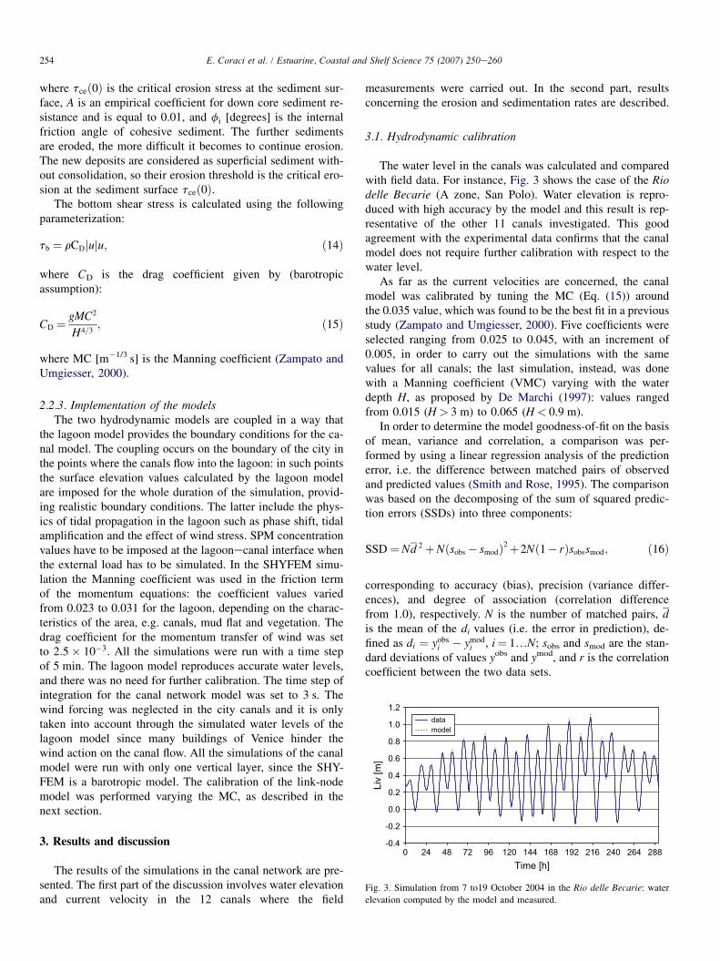
The water level in the canals was calculated and comparedwith field data. For instance, Fig. 3 shows the case of the Riodelle Becarie (A zone, San Polo). Water elevation is repro-duced with high accuracy by the model and this result is rep-resentative of the other 11 canals investigated. This goodagreement with the experimental data confirms that the canalmodel does not require further calibration with respect to thewater level.

As far as the current velocities are concerned, the canalmodel was calibrated by tuning the MC (Eq. (15)) aroundthe 0.035 value, which was found to be the best fit in a previousstudy (Zampato and Umgiesser, 2000). Five coefficients wereselected ranging from 0.025 to 0.045, with an increment of0.005, in order to carry out the simulations with the samevalues for all canals; the last simulation, instead, was donewith a Manning coefficient (VMC) varying with the waterdepth H, as proposed by De Marchi (1997): values rangedfrom 0.015 (H> 3 m) to 0.065 (H< 0.9 m).

In order to determine the model goodness-of-fit on the basisof mean, variance and correlation, a comparison was per-formed by using a linear regression analysis of the predictionerror, i.e. the difference between matched pairs of observedand predicted values (Smith and Rose, 1995). The comparisonwas based on the decomposing of the sum of squared predic-tion errors (SSDs) into three components:

SSD¼ Nd 2þNðsobs � smodÞ2þ2Nð1� rÞsobssmod; ð16Þ

corresponding to accuracy (bias), precision (variance differ-ences), and degree of association (correlation differencefrom 1.0), respectively. N is the number of matched pairs, dis the mean of the di values (i.e. the error in prediction), de-fined as di ¼ yobs

i � ymodi , i¼ 1.N; sobs and smod are the stan-

dard deviations of values yobs and ymod, and r is the correlationcoefficient between the two data sets.

-0.4

-0.2

0.0

0.2

0.4

0.6

0.8

1.0

1.2

0 24 48 72 96 120 144 168 192 216 240 264 288Time [h]

Liv

[m]

datamodel

Fig. 3. Simulation from 7 to19 October 2004 in the Rio delle Becarie: water

elevation computed by the model and measured.


The statistical results are represented in a 2D plot on whichthe correlation coefficient and the root-mean-square differencebetween the two data sets (observed and calculated) are indi-cated by a single point (Taylor, 2001). This type of diagramsummarizes the degree of correspondence between the fielddata and the model. In fact, Taylor proposed a similar methodto quantify the differences in two data sets using the root-mean-square difference E, defined as:

E¼

ffiffiffiffiffiffiffiffiffiffiffiffiffiffiffiffiffiffiffiffiffiffiffiffiffiffiffiffiffiffiffiffiffiffiffiffiffiPNi¼1ðyi

obs � yimodÞ

2

N:

sð17Þ

The quantity E can be resolved into two components to iso-late differences in phase and amplitude from differences in themeans of the two fields:

E2 ¼ d 2þE02; ð18Þ

where d is the bias, and E0 is computed by standard deviationsand the correlation coefficient, which are the second and thirdterms in Eq. (16) Therefore Eqs. (16) and (18) are equivalentwith the exception of a factor N.

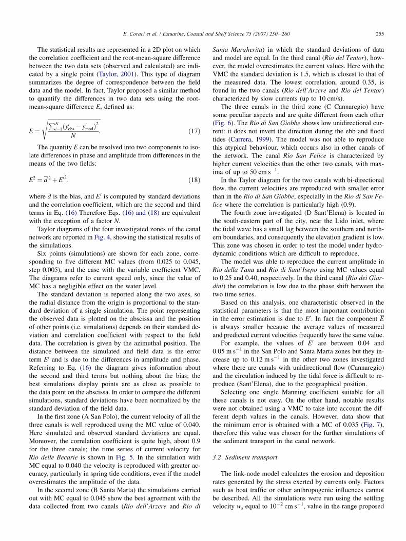
Taylor diagrams of the four investigated zones of the canalnetwork are reported in Fig. 4, showing the statistical results ofthe simulations.

Six points (simulations) are shown for each zone, corre-sponding to five different MC values (from 0.025 to 0.045,step 0.005), and the case with the variable coefficient VMC.The diagrams refer to current speed only, since the value ofMC has a negligible effect on the water level.

The standard deviation is reported along the two axes, sothe radial distance from the origin is proportional to the stan-dard deviation of a single simulation. The point representingthe observed data is plotted on the abscissa and the positionof other points (i.e. simulations) depends on their standard de-viation and correlation coefficient with respect to the fielddata. The correlation is given by the azimuthal position. Thedistance between the simulated and field data is the errorterm E0 and is due to the differences in amplitude and phase.Referring to Eq. (16) the diagram gives information aboutthe second and third terms but nothing about the bias; thebest simulations display points are as close as possible tothe data point on the abscissa. In order to compare the differentsimulations, standard deviations have been normalized by thestandard deviation of the field data.

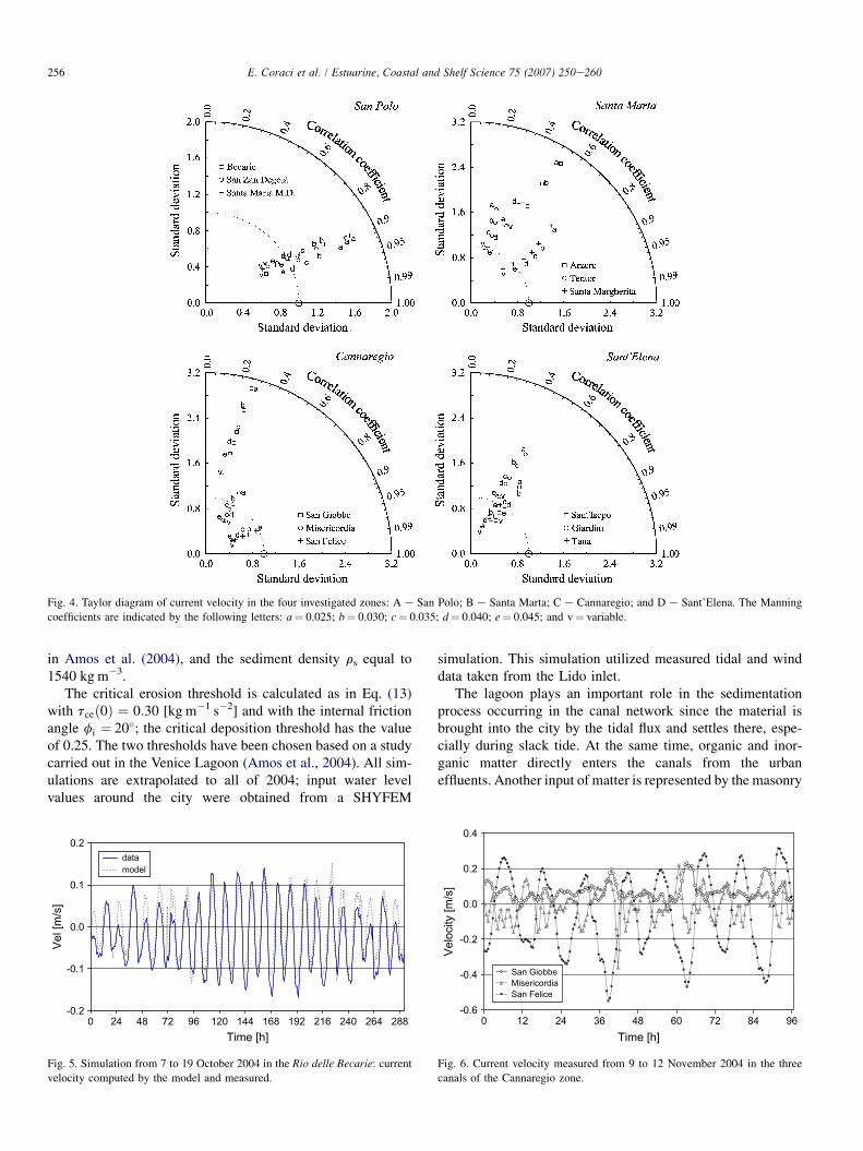
In the first zone (A San Polo), the current velocity of all thethree canals is well reproduced using the MC value of 0.040.Here simulated and observed standard deviations are equal.Moreover, the correlation coefficient is quite high, about 0.9for the three canals; the time series of current velocity forRio delle Becarie is shown in Fig. 5. In the simulation withMC equal to 0.040 the velocity is reproduced with greater ac-curacy, particularly in spring tide conditions, even if the modeloverestimates the amplitude of the data.

In the second zone (B Santa Marta) the simulations carriedout with MC equal to 0.045 show the best agreement with thedata collected from two canals (Rio dell’Arzere and Rio di

Santa Margherita) in which the standard deviations of dataand model are equal. In the third canal (Rio del Tentor), how-ever, the model overestimates the current values. Here with theVMC the standard deviation is 1.5, which is closest to that ofthe measured data. The lowest correlation, around 0.35, isfound in the two canals (Rio dell’Arzere and Rio del Tentor)characterized by slow currents (up to 10 cm/s).

The three canals in the third zone (C Cannaregio) havesome peculiar aspects and are quite different from each other(Fig. 6). The Rio di San Giobbe shows low unidirectional cur-rent: it does not invert the direction during the ebb and floodtides (Carrera, 1999). The model was not able to reproducethis atypical behaviour, which occurs also in other canals ofthe network. The canal Rio San Felice is characterized byhigher current velocities than the other two canals, with max-ima of up to 50 cm s�1.

In the Taylor diagram for the two canals with bi-directionalflow, the current velocities are reproduced with smaller errorthan in the Rio di San Giobbe, especially in the Rio di San Fe-lice where the correlation is particularly high (0.9).

The fourth zone investigated (D Sant’Elena) is located inthe south-eastern part of the city, near the Lido inlet, wherethe tidal wave has a small lag between the southern and north-ern boundaries, and consequently the elevation gradient is low.This zone was chosen in order to test the model under hydro-dynamic conditions which are difficult to reproduce.

The model was able to reproduce the current amplitude inRio della Tana and Rio di Sant’Isepo using MC values equalto 0.25 and 0.40, respectively. In the third canal (Rio dei Giar-dini) the correlation is low due to the phase shift between thetwo time series.

Based on this analysis, one characteristic observed in thestatistical parameters is that the most important contributionin the error estimation is due to E0. In fact the component Eis always smaller because the average values of measuredand predicted current velocities frequently have the same value.

For example, the values of E0 are between 0.04 and0.05 m s�1 in the San Polo and Santa Marta zones but they in-crease up to 0.12 m s�1 in the other two zones investigatedwhere there are canals with unidirectional flow (Cannaregio)and the circulation induced by the tidal force is difficult to re-produce (Sant’Elena), due to the geographical position.

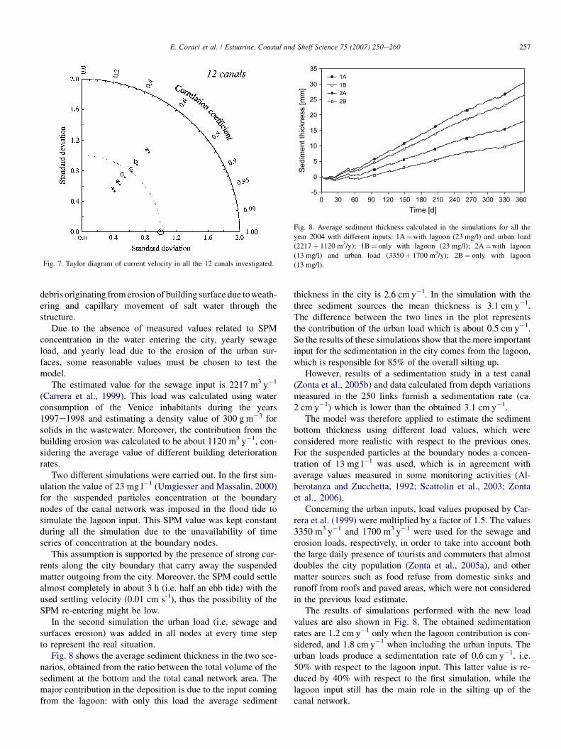
Selecting one single Manning coefficient suitable for allthese canals is not easy. On the other hand, notable resultswere not obtained using a VMC to take into account the dif-ferent depth values in the canals. However, data show thatthe minimum error is obtained with a MC of 0.035 (Fig. 7),therefore this value was chosen for the further simulations ofthe sediment transport in the canal network.

3.2. Sediment transport

The link-node model calculates the erosion and depositionrates generated by the stress exerted by currents only. Factorssuch as boat traffic or other anthropogenic influences cannotbe described. All the simulations were run using the settlingvelocity ws equal to 10�2 cm s�1, value in the range proposed


Fig. 4. Taylor diagram of current velocity in the four investigated zones: A e San Polo; B e Santa Marta; C e Cannaregio; and D e Sant’Elena. The Manning

coefficients are indicated by the following letters: a¼ 0.025; b¼ 0.030; c¼ 0.035; d¼ 0.040; e¼ 0.045; and v¼ variable.

in Amos et al. (2004), and the sediment density rs equal to1540 kg m�3.

The critical erosion threshold is calculated as in Eq. (13)with tceð0Þ ¼ 0:30 [kg m�1 s�2] and with the internal frictionangle fi ¼ 20�; the critical deposition threshold has the valueof 0.25. The two thresholds have been chosen based on a studycarried out in the Venice Lagoon (Amos et al., 2004). All sim-ulations are extrapolated to all of 2004; input water levelvalues around the city were obtained from a SHYFEM

-0.2

-0.1

0.0

0.1

0.2

0 24 48 72 96 120 144 168 192 216 240 264 288Time [h]

Vel [

m/s

]

datamodel

Fig. 5. Simulation from 7 to 19 October 2004 in the Rio delle Becarie: current

velocity computed by the model and measured.

simulation. This simulation utilized measured tidal and winddata taken from the Lido inlet.

The lagoon plays an important role in the sedimentationprocess occurring in the canal network since the material isbrought into the city by the tidal flux and settles there, espe-cially during slack tide. At the same time, organic and inor-ganic matter directly enters the canals from the urbaneffluents. Another input of matter is represented by the masonry

-0.6

-0.4

-0.2

0.0

0.2

0.4

0 12 24 36 48 60 72 84 96Time [h]

Velo

city

[m/s

]

San GiobbeMisericordiaSan Felice

Fig. 6. Current velocity measured from 9 to 12 November 2004 in the three

canals of the Cannaregio zone.


debris originating from erosion of building surface due to weath-ering and capillary movement of salt water through thestructure.

Due to the absence of measured values related to SPMconcentration in the water entering the city, yearly sewageload, and yearly load due to the erosion of the urban sur-faces, some reasonable values must be chosen to test themodel.

The estimated value for the sewage input is 2217 m3 y�1

(Carrera et al., 1999). This load was calculated using waterconsumption of the Venice inhabitants during the years1997e1998 and estimating a density value of 300 g m�3 forsolids in the wastewater. Moreover, the contribution from thebuilding erosion was calculated to be about 1120 m3 y�1, con-sidering the average value of different building deteriorationrates.

Two different simulations were carried out. In the first sim-ulation the value of 23 mg l�1 (Umgiesser and Massalin, 2000)for the suspended particles concentration at the boundarynodes of the canal network was imposed in the flood tide tosimulate the lagoon input. This SPM value was kept constantduring all the simulation due to the unavailability of timeseries of concentration at the boundary nodes.

This assumption is supported by the presence of strong cur-rents along the city boundary that carry away the suspendedmatter outgoing from the city. Moreover, the SPM could settlealmost completely in about 3 h (i.e. half an ebb tide) with theused settling velocity (0.01 cm s-1), thus the possibility of theSPM re-entering might be low.

In the second simulation the urban load (i.e. sewage andsurfaces erosion) was added in all nodes at every time stepto represent the real situation.

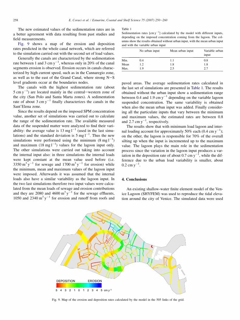
Fig. 8 shows the average sediment thickness in the two sce-narios, obtained from the ratio between the total volume of thesediment at the bottom and the total canal network area. Themajor contribution in the deposition is due to the input comingfrom the lagoon: with only this load the average sediment

Fig. 7. Taylor diagram of current velocity in all the 12 canals investigated.

thickness in the city is 2.6 cm y�1. In the simulation with thethree sediment sources the mean thickness is 3.1 cm y�1.The difference between the two lines in the plot representsthe contribution of the urban load which is about 0.5 cm y�1.So the results of these simulations show that the more importantinput for the sedimentation in the city comes from the lagoon,which is responsible for 85% of the overall silting up.

However, results of a sedimentation study in a test canal(Zonta et al., 2005b) and data calculated from depth variationsmeasured in the 250 links furnish a sedimentation rate (ca.2 cm y�1) which is lower than the obtained 3.1 cm y�1.

The model was therefore applied to estimate the sedimentbottom thickness using different load values, which wereconsidered more realistic with respect to the previous ones.For the suspended particles at the boundary nodes a concen-tration of 13 mg l�1 was used, which is in agreement withaverage values measured in some monitoring activities (Al-berotanza and Zucchetta, 1992; Scattolin et al., 2003; Zontaet al., 2006).

Concerning the urban inputs, load values proposed by Car-rera et al. (1999) were multiplied by a factor of 1.5. The values3350 m3 y�1 and 1700 m3 y�1 were used for the sewage anderosion loads, respectively, in order to take into account boththe large daily presence of tourists and commuters that almostdoubles the city population (Zonta et al., 2005a), and othermatter sources such as food refuse from domestic sinks andrunoff from roofs and paved areas, which were not consideredin the previous load estimate.

The results of simulations performed with the new loadvalues are also shown in Fig. 8. The obtained sedimentationrates are 1.2 cm y�1 only when the lagoon contribution is con-sidered, and 1.8 cm y�1 when including the urban inputs. Theurban loads produce a sedimentation rate of 0.6 cm y�1, i.e.50% with respect to the lagoon input. This latter value is re-duced by 40% with respect to the first simulation, while thelagoon input still has the main role in the silting up of thecanal network.

-5

0

5

10

15

20

25

30

35

0 30 60 90 120 150 180 210 240 270 300 330 360Time [d]

Sedi

men

t thi

ckne

ss [m

m]

1A1B2A2B

Fig. 8. Average sediment thickness calculated in the simulations for all the

year 2004 with different inputs: 1A¼with lagoon (23 mg/l) and urban load

(2217þ 1120 m3/y); 1B¼ only with lagoon (23 mg/l); 2A¼with lagoon

(13 mg/l) and urban load (3350þ 1700 m3/y); 2B¼ only with lagoon

(13 mg/l).


The new estimated values of the sedimentation rates are ina better agreement with data resulting from past studies andfield measurements.

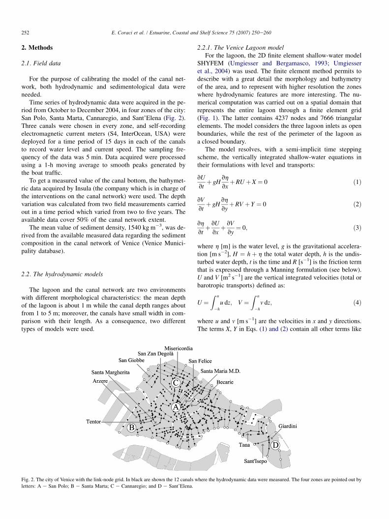
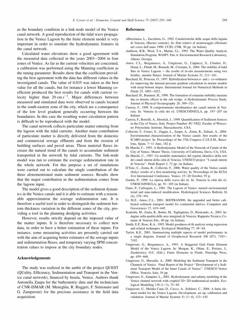
Fig. 9 shows a map of the erosion and depositionrates predicted in the whole canal network, which are referredto the simulation carried out with the second set of load values.

Generally the canals are characterized by the sedimentationrate between 1 and 3 cm y�1, whereas only in 20% of the canalsegments erosion is observed. Erosion occurs in canals charac-terized by high current speed, such as in the Cannaregio zone,as well as to the east of the Grand Canal, where strong NeSlevel gradients occur at the boundaries nodes.

The canals with the highest sedimentation rate (about5 cm y�1) are located mainly in the centralewestern zone ofthe city (San Polo and Santa Marta zones). A sedimentationrate of about 3 cm y�1 finally characterizes the canals in theSant’Elena zone.

Since the results depend on the imposed SPM concentrationvalue, another set of simulations was carried out to calculatethe range of the sedimentation rate. The available measureddata of the suspended matter were analyzed to find their vari-ability: the average value is 13 mg l�1 (used in the last simu-lations) and the standard deviation is 5 mg l�1. Thus the newsimulations were performed using the minimum (8 mg l�1)and maximum (18 mg l�1) values for the lagoon input only.The other simulations were carried out taking into accountthe internal input also: in three simulations the internal loadswere kept constant at the mean value used before (i.e.3350 m3 y�1 for sewage and 1700 m3 y�1 for erosion) whilethe minimum, mean and maximum values of the lagoon inputwere imposed. Afterwards it was assumed that the internalloads also have a similar variability as the lagoon input. Inthe two last simulations therefore two input values were calcu-lated from the mean loads of sewage and erosion contributionsand they are 2080 and 4600 m3 y�1 for the sewage effluents,1050 and 2340 m3 y�1 for erosion and runoff from roofs and

paved areas. The average sedimentation rates calculated inthe last set of simulations are presented in Table 1. The resultsobtained without the urban input show a sedimentation rangebetween 0.4 and 1.9 cm y�1 depending on the variable lagoonsuspended concentration. The same variability is obtainedwhen also the mean urban input was added. Finally consider-ing all the particulate inputs that vary between the minimumand maximum values, the estimated rates are between 0.8and 2.7 cm y�1, respectively.

The results show that with minimum load lagoon and inter-nal loading account for approximately 50% each (0.4 cm y�1);on the other, the lagoon is responsible for 70% of the overallsilting up when the input is incremented up to the maximumvalue. The lagoon plays the main role in the sedimentationprocess since the variation in the lagoon input produces a var-iation in the deposition rate of about 0.7 cm y�1, while the dif-ference due to the urban load variability is smaller, about0.2 cm y�1.

4. Conclusions

An existing shallow-water finite element model of the Ven-ice Lagoon (SHYFEM) was used to reproduce the tidal eleva-tion around the city of Venice. The simulated data were used

Table 1

Sedimentation rates [cm y�1] calculated by the model with different inputs,

depending on the imposed concentration coming from the lagoon. The col-

umns show the results obtained without urban input, with the mean urban input

and with the variable urban input

No urban input Mean urban input Variable urban

input

Min. 0.4 1.1 0.8

Mean 1.2 1.8 1.8

Max. 1.9 2.5 2.7

Fig. 9. Map of the erosion and deposition rates calculated by the model in the 505 links of the grid.


as the boundary condition in a link-node model of the Venicecanal network. A good reproduction of the tidal wave propaga-tion in the Venice Lagoon by the finite element model is veryimportant in order to simulate the hydrodynamic features inthe canal network.

Calculated water elevations show a good agreement withthe measured data collected in the years 2003e2004 in fourzones of Venice. As far as the current velocities are concerned,a calibration was performed using the Manning coefficient asthe tuning parameter. Results show that the coefficient provid-ing the best agreement with the data has different values in theinvestigated canals. The value of 0.035 was taken as the bestvalue for all the canals, but for instance a lower Manning co-efficient produced the best results for canals with current ve-locity higher than 20 cm s�1. Major differences betweenmeasured and simulated data were observed in canals locatedin the south-eastern zone of the city, which are a consequenceof the low level gradient generally occurring between theboundaries. In this case the resulting water circulation patternis difficult to be reproduced with the model.

The canal network collects particulate matter entering fromthe lagoon with the tidal currents. Another main contributionof particulate matter is directly delivered from the domesticand commercial sewage effluents and from the erosion ofbuilding surfaces and paved areas. These material fluxes in-crease the natural trend of the canals to accumulate sedimenttransported in the network by tidal currents. The link-nodemodel was run to estimate the average sedimentation rate inthe whole network. For this purpose a set of simulationswere carried out to calculate the single contribution of thethree aforementioned main sediment sources. Results showthat the major contribution in the sedimentation comes fromthe lagoon input.

The model gives a good description of the sediment dynam-ics in the Venice canals and it is able to estimate with a reason-able approximation the average sedimentation rate. It istherefore a useful tool in order to distinguish the sediment bot-tom thickness variation in the different zones of the city, pro-viding a tool in the planning dredging activities.

However, results strictly depend on the imposed value ofthe matter inputs. It is therefore necessary to collect newdata, in order to have a better estimation of these inputs. Forinstance, some measuring activities are presently carried outwith the aim of acquiring better estimates of the sewage inputsand sedimentation fluxes, and temporary varying SPM concen-tration values to impose at the city boundary nodes.

Acknowledgements

The study was realized in the ambit of the project QUEST(QUality, Efficiency, Sedimentation and Transport in the Ven-ice canal network), financed by Insula, Venice. Authors thankAntonella Zaupa for the bathymetric data and the techniciansof CNR-ISMAR (M. Meneghin, R. Ruggeri, F. Simionato andG. Zamperoni) for the precious assistance in the field dataacquisition.

References

Alberotanza, L., Zucchetta, G., 1992. Caratteristiche delle acque della laguna

di Venezia, (Bacino centrale). In: Dati relativi al monitoraggio effettuato

nel corso dell’anno 1990. CCID, CNR, 50 pp. (in Italian).

Ambrose, R.B., Wool, T.A., Martin, J.L., 1993. The Water Quality Analysis

Simulation Program, WASP5. Part A. Environmental Research Laboratory,

Athens, Georgia.

Amos, C.L., Bergamasco, A., Umgiesser, G., Cappucci, S., Cloutier, D.,

Denat, L., Flindt, M., Bonardi, M., Cristante, S., 2004. The stability of tidal

flats in Venice Lagoon e the results of in-situ measurements using two

benthic, annular flumes. Journal of Marine Systems 51, 211e241.

Burchard, H., Petersen, O., 1997. Hybridization between s- and z- co-ordinates

for improving the internal pressure gradient calculation in marine models

with steep bottom slopes. International Journal for Numerical Methods in

Fluids 25, 1003e1023.

Burchard, H., Baumert, H., 1998. The formation of estuarine turbidity maxima

due to density effects in the salt wedge. A Hydrodynamic Process Study.

Journal of Physical Oceanography 28, 309e321.

Carrera, F., 1999. Il comportamento idrodinamico dei canali interni di Ven-

ezia. In: Venezia la citta dei rii. UNESCO/INSULA, pp. 197e207 (in

Italian).

Carrera, F., Borrelli, A., Horstick, J., 1999. Quantification of Sediment Sources

in the City of Venice, Italy. Project Number: FC-VEI2. Faculty of Worces-

ter Polytechnic Institute, Massachusetts, USA.

Collavini, F., Coraci, E., Zaggia, L., Zaupa, A., Zonta, R., Zuliani, A., 2004.

Environmental characterisation of the Venice canals: first results of the

ICARO project. In: Proceedings of the 37th Congress C.I.E.S.M., Barce-

lona, Spain, 7e11 June, 182 p.

De Marchi, C., 1993. A Hydrodynamic Model of the Network of Canals of the

City of Venice. Master Thesis, University of California, Davis, CA, USA.

De Marchi, C., 1997. Un modello matematico del regime idraulico della rete

dei canali interni della citta di Venezia. UNESCO project ‘‘I canali interni

di Venezia’’. Draft Report 2, 72 pp. (in Italian).

D’Este, C., Zonta, R., Collavini, F., 2006. Water quality of the Venice canals

(Italy): results of a first monitoring activity. In: Proceedings of the ECSA

41st International Conference, Venice, 15e20 October, 93 p.

Gardin, P., 1999. La ripresa dello scavo dei rii. In: Venezia la citta dei rii.

UNESCO/INSULA, pp. 91e105 (in Italian).

Gatto, P., Carbognin, L., 1981. The Lagoon of Venice: natural environmental

trend and man-induced modification. Hydrological Sciences Bulletin 26

(4), 379e391.

Li, M.Z., Amos, C.L., 2001. SEDTRANS96: the upgraded and better cali-

brated sediment transport model for continental shelves. Computers and

Geosciences 27, 619e645.

Scattolin, M., Zonta, R., Botter, M., Tagliapietra, D., Rismondo, A., 2003. In-

dagine sulla qualita delle aree marginali di Venezia. Rapporto Tecnico, Co-

mune di Venezia Eds., 80 pp. (in Italian).

Smith, E.P., Rose, K.A., 1995. Model goodness-of-fit analysis using regression

and related techniques. Ecological Modelling 77, 49e64.

Taylor, K.E., 2001. Summarizing multiple aspects of model performance in

a single diagram. Journal of Geophysical Research 106 (D7), 7183e

7192.

Umgiesser, G., Bergamasco, A., 1993. A Staggered Grid Finite Element

Model of the Venice Lagoon. In: Morgan, K., Ofiate, E., Periaux, J.,

Zienkiewicz, O.C. (Eds.), Finite Elements in Fluids. Pineridge Press,

pp. 659e668.

Umgiesser, G., Massalin, A., 2000. Modeling the Sediment Transport in the

Channels of Venice. Final Report of the Project ‘‘Development of a Sedi-

ment Transport Model of the Inner Canals of Venice’’. UNESCO Venice

Office, Venezia, Italy, 54 pp.

Umgiesser, G., Zampato, L., 2001. Hydrodynamic and salinity modeling of the

Venice channel network with coupled 1De2D mathematical models. Eco-

logical Modelling 138 (1e3), 75e85.

Umgiesser, G., Melaku Canu, D., Cucco, A., Solidoro, C., 2004. A finite ele-

ment model for the Venice Lagoon. Development, set up, calibration and

validation. Journal of Marine Systems 51 (1e4), 123e145.


Zampato, L., Umgiesser, G., 2000. Hydrodynamic modeling in the channel

network of Venice. Il Nuovo Cimento C 23 (3), 263e284.

Zonta, R., Zaggia, L., Collavini, F., Costa, F., Scattolin, M., 2005a. Sediment

contamination assessment of the Venice canal network (Italy). In:

Fletcher, C.A., Spencer, T. (Eds.), Flooding and Environmental Challenges

for Venice and Its Lagoon: State of Knowledge. Cambridge University

Press, pp. 603e615.

Zonta, R., Cochran, J.K., Collavini, F., Costa, F., Scattolin, M., Zaggia, L.,

2005b. Sediment and heavy metal accumulation in a small canal, Venice,

Italy. Aquatic Ecosystem Health & Management 8 (1), 63e71.

Zonta, R., Zuliani, A., Coraci, E., D’Este, C., Pesce, A., 2006. Fluxes of par-

ticulate, metals and nutrients in a test canal of Venice (Italy). In: Proceed-

ings of the ECSA 41st International Conference, Venice, 15e20 October,

106 p.

Documents

Hydrodynamic and sediment transport modelling in the canals of Venice (Italy)