Embed Size (px)
DESCRIPTION
04/04/2006. Hydrologic Statistics. Reading: Chapter 11, Sections 12-1 and 12-2 of Applied Hydrology. Probability. A measure of how likely an event will occur A number expressing the ratio of favorable outcome to the all possible outcomes Probability is usually represented as P(.) - PowerPoint PPT Presentation
Citation preview
Hydrologic Statistics
Reading: Chapter 11, Sections 12-1 and 12-2 of Applied Hydrology
04/04/2006
2
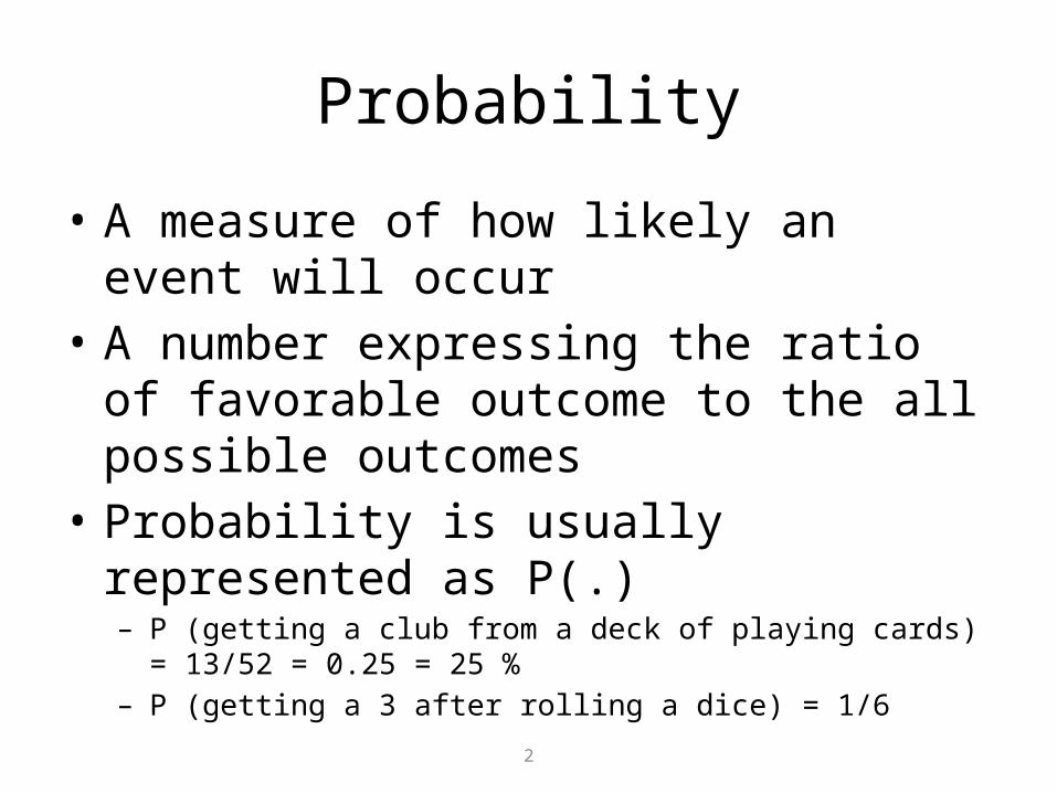
Probability
• A measure of how likely an event will occur• A number expressing the ratio of favorable
outcome to the all possible outcomes • Probability is usually represented as P(.)
– P (getting a club from a deck of playing cards) = 13/52 = 0.25 = 25 %– P (getting a 3 after rolling a dice) = 1/6
3
Random Variable
• Random variable: a quantity used to represent probabilistic uncertainty– Incremental precipitation – Instantaneous streamflow– Wind velocity
• Random variable (X) is described by a probability distribution
• Probability distribution is a set of probabilities associated with the values in a random variable’s sample space
5
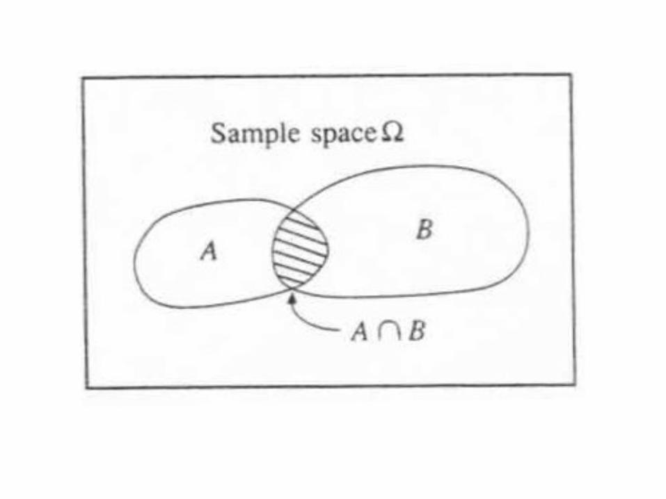
Sampling terminology• Sample: a finite set of observations x1, x2,….., xn of the random
variable• A sample comes from a hypothetical infinite population
possessing constant statistical properties• Sample space: set of possible samples that can be drawn from a
population• Event: subset of a sample space Example
Population: streamflow Sample space: instantaneous streamflow, annual
maximum streamflow, daily average streamflow Sample: 100 observations of annual max. streamflow Event: daily average streamflow > 100 cfs
6
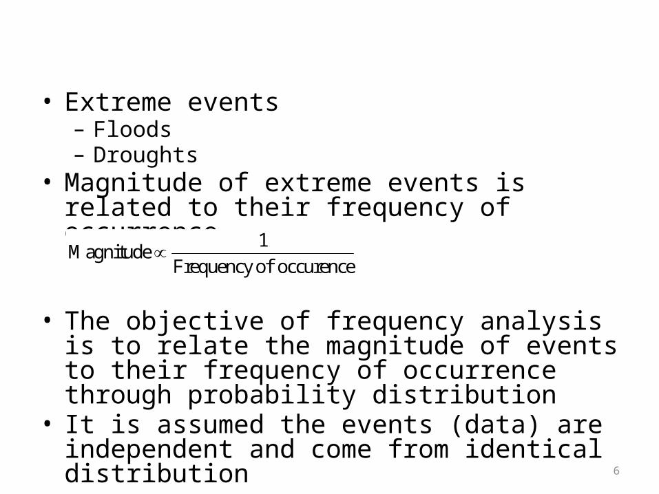
Hydrologic extremes
• Extreme events– Floods – Droughts
• Magnitude of extreme events is related to their frequency of occurrence
• The objective of frequency analysis is to relate the magnitude of events to their frequency of occurrence through probability distribution
• It is assumed the events (data) are independent and come from identical distribution
occurence ofFrequency
1Magnitude
7
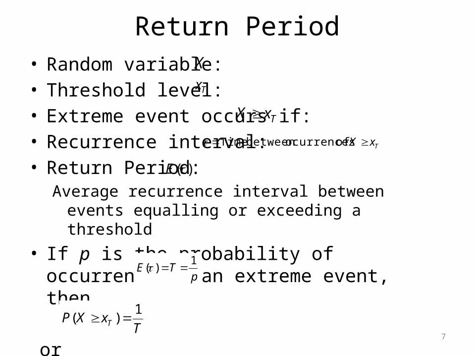
Return Period• Random variable:• Threshold level:• Extreme event occurs if: • Recurrence interval: • Return Period:
Average recurrence interval between events equalling or exceeding a threshold
• If p is the probability of occurrence of an extreme event, then
or
TxX
Tx
X
TxX of ocurrencesbetween Time
)(E
pTE
1)(
TxXP T
1)(
8
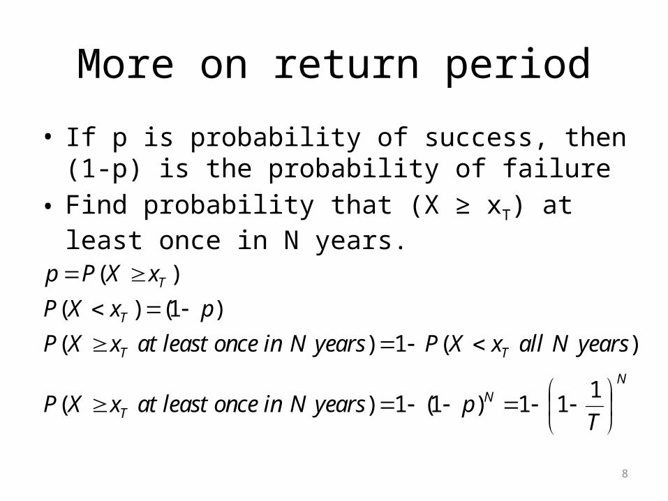
More on return period
• If p is probability of success, then (1-p) is the probability of failure
• Find probability that (X ≥ xT) at least once in N years.
NN
T
TT
T
T
TpyearsNinonceleastatxXP
yearsNallxXPyearsNinonceleastatxXP
pxXP
xXPp
111)1(1)(
)(1)(
)1()(
)(
9
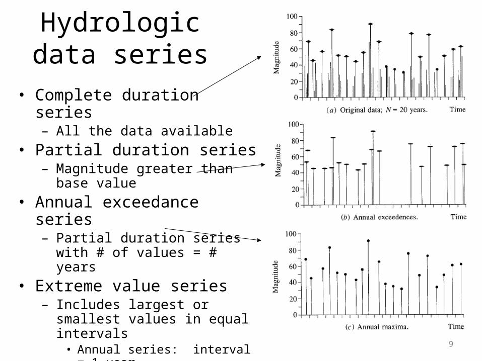
Hydrologic data series
• Complete duration series– All the data available
• Partial duration series– Magnitude greater than base value
• Annual exceedance series– Partial duration series with # of
values = # years• Extreme value series
– Includes largest or smallest values in equal intervals
• Annual series: interval = 1 year• Annual maximum series: largest
values• Annual minimum series : smallest
values
10
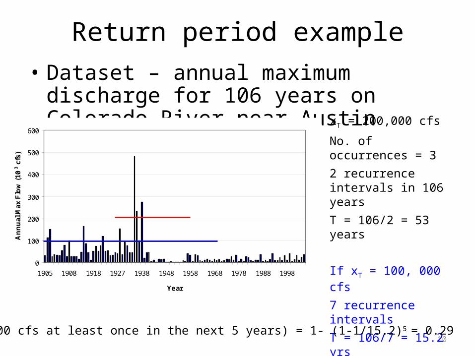
Return period example• Dataset – annual maximum discharge for 106
years on Colorado River near Austin
0
100
200
300
400
500
600
1905 1908 1918 1927 1938 1948 1958 1968 1978 1988 1998
Year
An
nu
al M
ax F
low
(10
3 c
fs)
xT = 200,000 cfs
No. of occurrences = 3
2 recurrence intervals in 106 years
T = 106/2 = 53 years
If xT = 100, 000 cfs
7 recurrence intervals
T = 106/7 = 15.2 yrs
P( X ≥ 100,000 cfs at least once in the next 5 years) = 1- (1-1/15.2)5 = 0.29
11
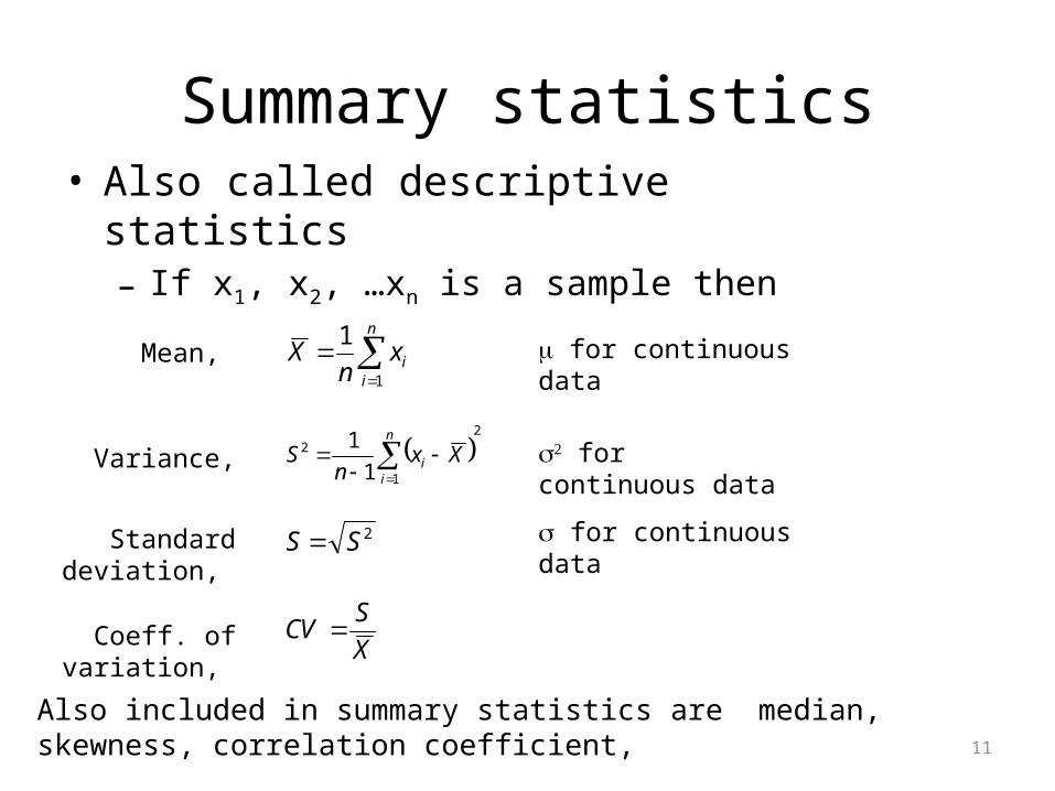
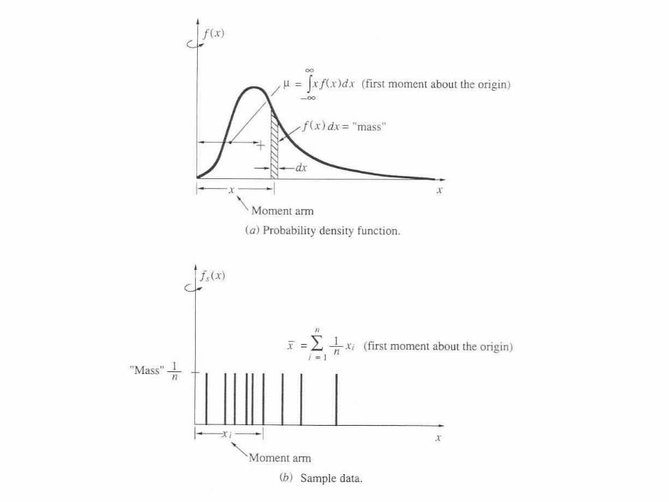
Summary statistics• Also called descriptive statistics
– If x1, x2, …xn is a sample then
n
iix
nX
1
1
2
1
2
1
1
n
ii Xx
nS
2SS
X
SCV
Mean,
Variance,
Standard deviation,
Coeff. of variation,
m for continuous data
s2 for continuous data
s for continuous data
Also included in summary statistics are median, skewness, correlation coefficient,
13
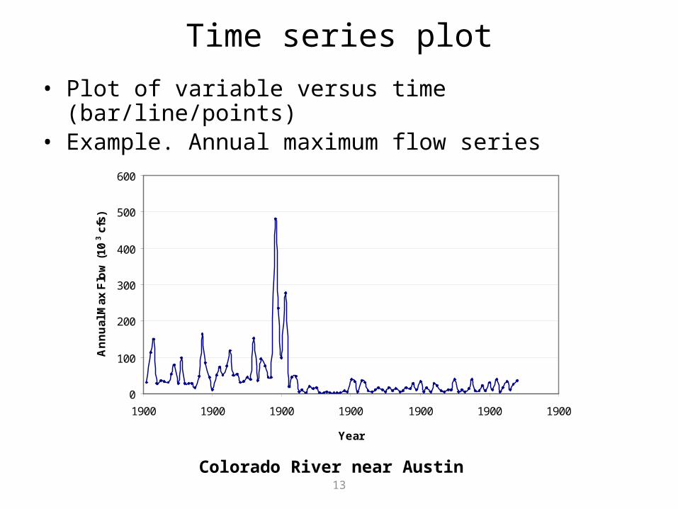
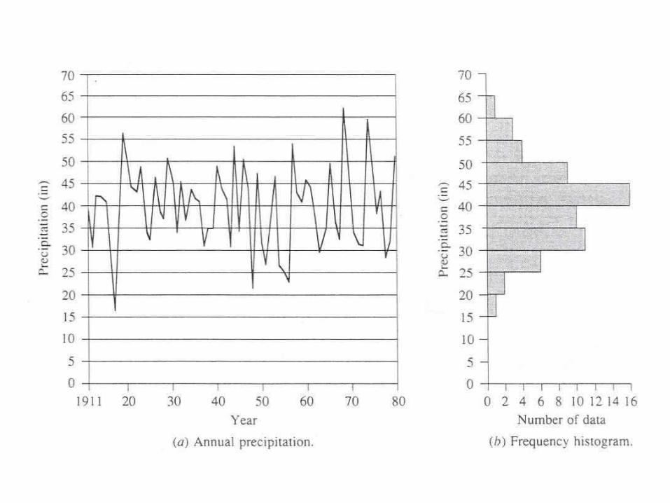
Time series plot• Plot of variable versus time (bar/line/points)• Example. Annual maximum flow series
0
100
200
300
400
500
600
1905 1908 1918 1927 1938 1948 1958 1968 1978 1988 1998
Year
An
nu
al M
ax F
low
(10
3 c
fs)
Colorado River near Austin
0
100
200
300
400
500
600
1900 1900 1900 1900 1900 1900 1900
Year
An
nu
al M
ax F
low
(10
3 c
fs)
14
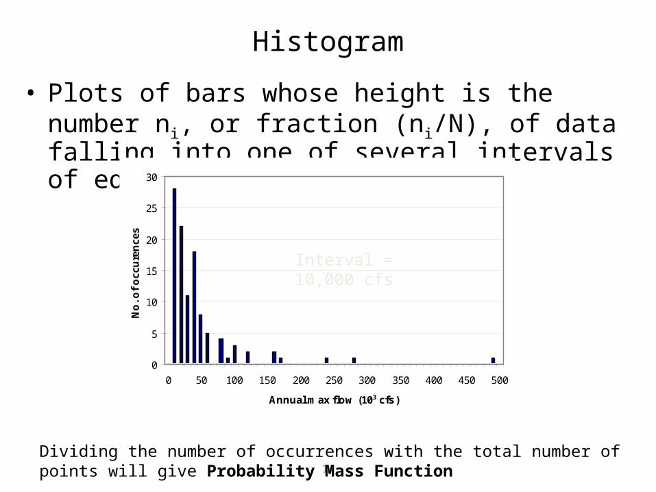
Histogram
• Plots of bars whose height is the number ni, or fraction (ni/N), of data falling into one of several intervals of equal width
0
10
20
30
40
50
60
70
80
90
100
0 50 100 150 200 250 300 350 400 450 500
Annual max flow (103 cfs)
No
. of
occ
ure
nce
s Interval = 50,000 cfs
0
10
20
30
40
50
60
Annual max flow (103 cfs)
No
. of
occ
ure
nce
s
Interval = 25,000 cfs
0
5
10
15
20
25
30
0 50 100 150 200 250 300 350 400 450 500
Annual max flow (103 cfs)
No
. of
occ
ure
nce
s
Interval = 10,000 cfs
Dividing the number of occurrences with the total number of points will give Probability Mass Function
16
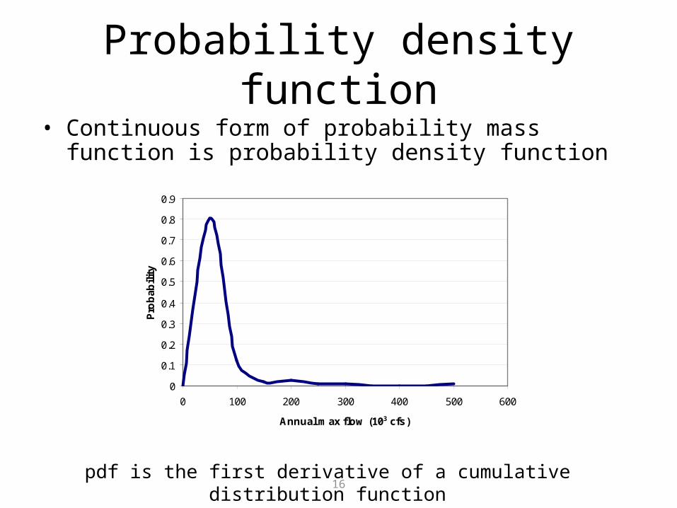
Probability density function• Continuous form of probability mass function is probability
density function
0
10
20
30
40
50
60
70
80
90
100
0 50 100 150 200 250 300 350 400 450 500
Annual max flow (103 cfs)
No
. of
occ
ure
nce
s
0
0.1
0.2
0.3
0.4
0.5
0.6
0.7
0.8
0.9
0 100 200 300 400 500 600
Annual max flow (103 cfs)
Pro
bab
ility
pdf is the first derivative of a cumulative distribution function
18
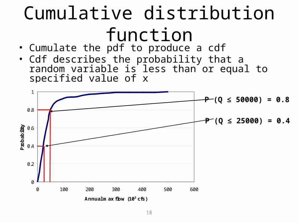
Cumulative distribution function• Cumulate the pdf to produce a cdf• Cdf describes the probability that a random variable is less
than or equal to specified value of x
0
0.2
0.4
0.6
0.8
1
0 100 200 300 400 500 600
Annual max flow (103 cfs)
Pro
bab
ility
P (Q ≤ 50000) = 0.8
P (Q ≤ 25000) = 0.4
22
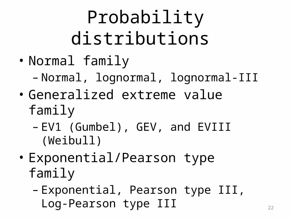
Probability distributions
• Normal family– Normal, lognormal, lognormal-III
• Generalized extreme value family– EV1 (Gumbel), GEV, and EVIII (Weibull)
• Exponential/Pearson type family– Exponential, Pearson type III, Log-Pearson type
III
23
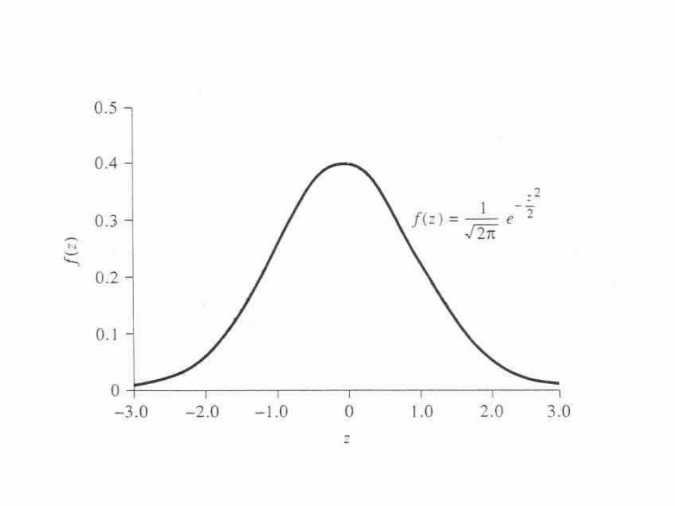
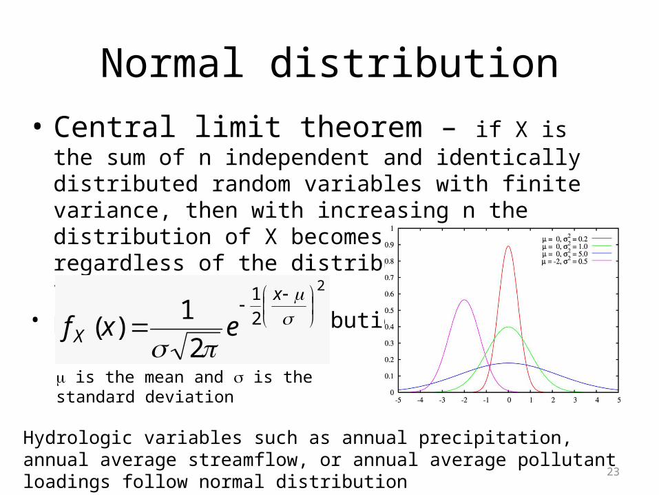
Normal distribution• Central limit theorem – if X is the sum of n
independent and identically distributed random variables with finite variance, then with increasing n the distribution of X becomes normal regardless of the distribution of random variables
• pdf for normal distribution2
2
1
2
1)(
sm
s
x
X exf
m is the mean and s is the standard deviation
Hydrologic variables such as annual precipitation, annual average streamflow, or annual average pollutant loadings follow normal distribution
24
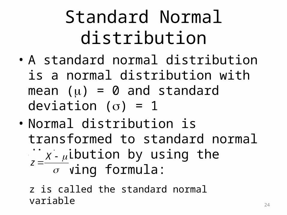
Standard Normal distribution
• A standard normal distribution is a normal distribution with mean (m) = 0 and standard deviation (s) = 1
• Normal distribution is transformed to standard normal distribution by using the following formula:
sm
X
z
z is called the standard normal variable
25
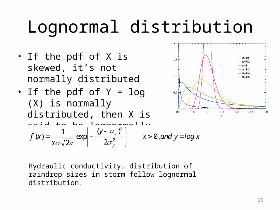
Lognormal distribution
• If the pdf of X is skewed, it’s not normally distributed
• If the pdf of Y = log (X) is normally distributed, then X is said to be lognormally distributed.
x log y and xy
xxf
y
y
,0
2
)(exp
2
1)(
2
2
sm
s
Hydraulic conductivity, distribution of raindrop sizes in storm follow lognormal distribution.
26
Extreme value (EV) distributions
• Extreme values – maximum or minimum values of sets of data
• Annual maximum discharge, annual minimum discharge
• When the number of selected extreme values is large, the distribution converges to one of the three forms of EV distributions called Type I, II and III
27
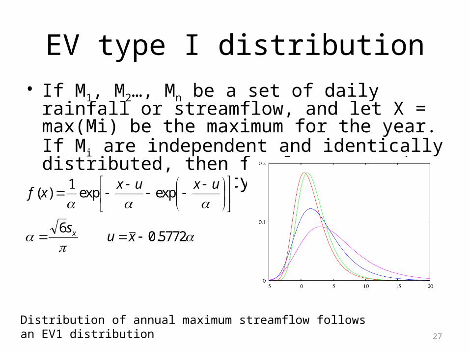
EV type I distribution• If M1, M2…, Mn be a set of daily rainfall or streamflow,
and let X = max(Mi) be the maximum for the year. If Mi are independent and identically distributed, then for large n, X has an extreme value type I or Gumbel distribution.
Distribution of annual maximum streamflow follows an EV1 distribution
5772.06
expexp1
)(
xus
uxuxxf
x
28
EV type III distribution
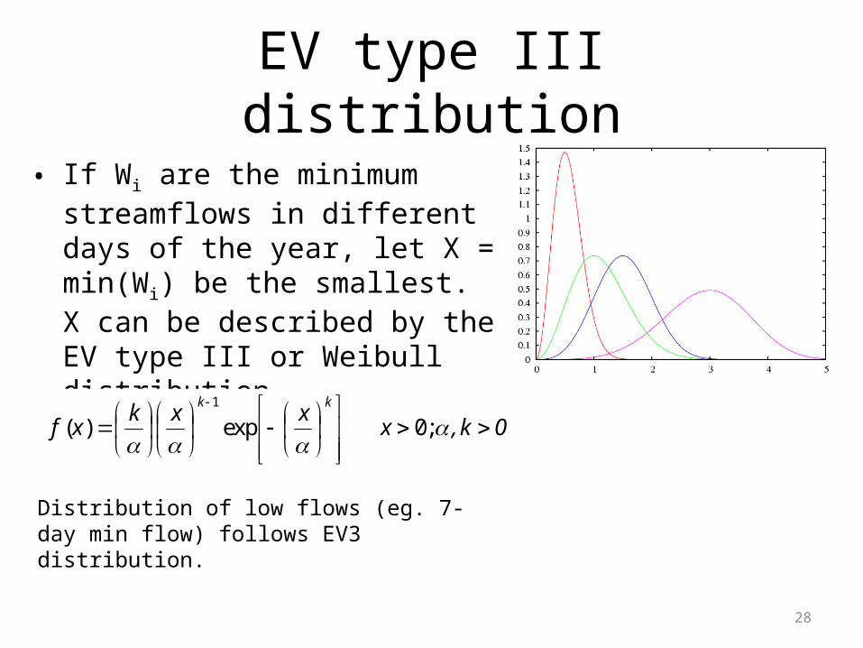
• If Wi are the minimum streamflows in different days of the year, let X = min(Wi) be the smallest. X can be described by the EV type III or Weibull distribution.
0k , xxxk
xfkk
;0exp)(1
Distribution of low flows (eg. 7-day min flow) follows EV3 distribution.
29
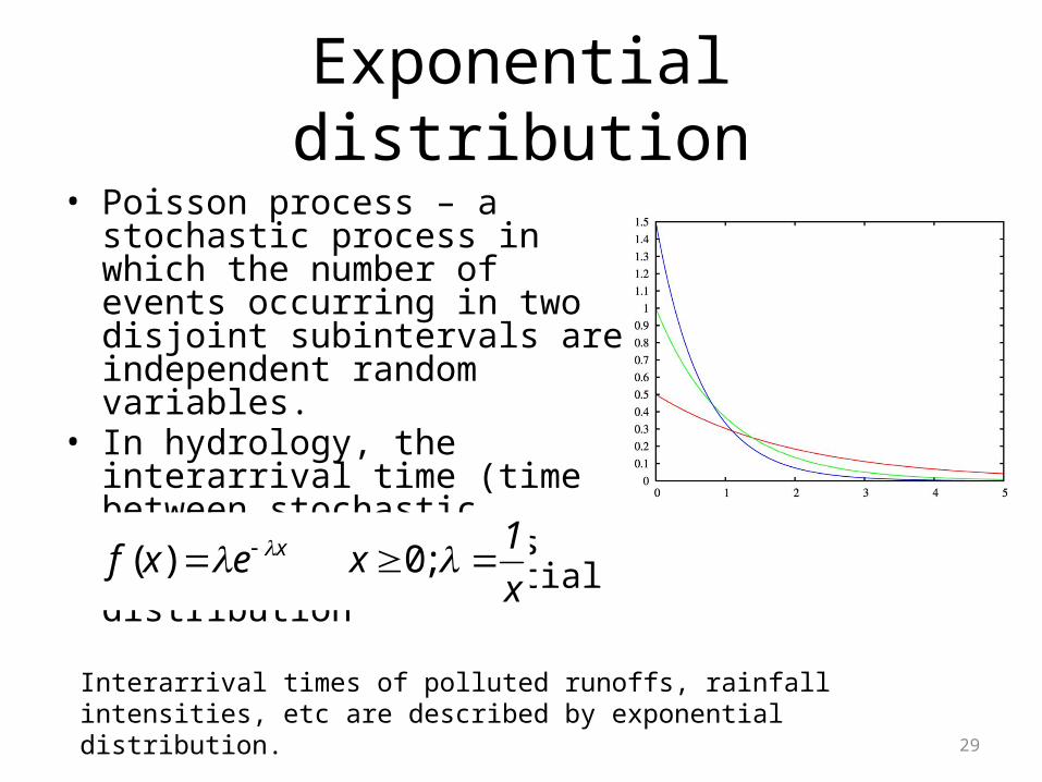
Exponential distribution• Poisson process – a stochastic
process in which the number of events occurring in two disjoint subintervals are independent random variables.
• In hydrology, the interarrival time (time between stochastic hydrologic events) is described by exponential distribution
x
1 xexf x ;0)(
Interarrival times of polluted runoffs, rainfall intensities, etc are described by exponential distribution.
30
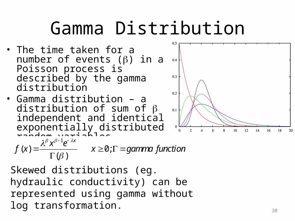
Gamma Distribution• The time taken for a number of
events (b) in a Poisson process is described by the gamma distribution
• Gamma distribution – a distribution of sum of b independent and identical exponentially distributed random variables.
Skewed distributions (eg. hydraulic conductivity) can be represented using gamma without log transformation.
function gamma xex
xfx
;0)(
)(1
31
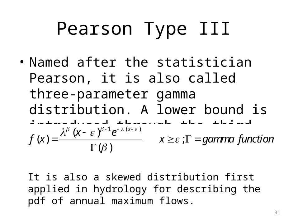
Pearson Type III
• Named after the statistician Pearson, it is also called three-parameter gamma distribution. A lower bound is introduced through the third parameter (e)
function gamma xex
xfx
;)(
)()(
)(1
It is also a skewed distribution first applied in hydrology for describing the pdf of annual maximum flows.
32
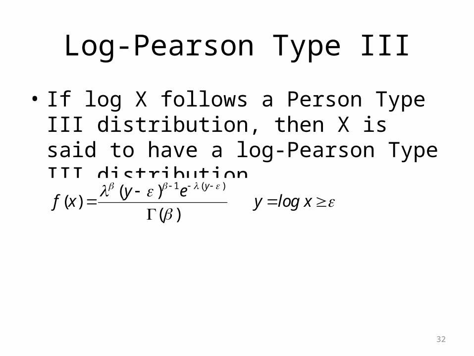
Log-Pearson Type III
• If log X follows a Person Type III distribution, then X is said to have a log-Pearson Type III distribution
x log yey
xfy
)(
)()(
)(1