Embed Size (px)
Citation preview
arX
iv:0
908.
3428
v1 [
mat
h.ST
] 2
4 A
ug 2
009
The Annals of Statistics
2009, Vol. 37, No. 5A, 2523–2542DOI: 10.1214/08-AOS651c© Institute of Mathematical Statistics, 2009
HYPOTHESIS TEST FOR NORMAL MIXTURE MODELS:
THE EM APPROACH
By Jiahua Chen1 and Pengfei Li
University of British Columbia and University of Alberta
Normal mixture distributions are arguably the most importantmixture models, and also the most technically challenging. The likeli-hood function of the normal mixture model is unbounded based on aset of random samples, unless an artificial bound is placed on its com-ponent variance parameter. Moreover, the model is not strongly iden-tifiable so it is hard to differentiate between over dispersion causedby the presence of a mixture and that caused by a large variance, andit has infinite Fisher information with respect to mixing proportions.There has been extensive research on finite normal mixture models,but much of it addresses merely consistency of the point estimationor useful practical procedures, and many results require undesirablerestrictions on the parameter space. We show that an EM-test forhomogeneity is effective at overcoming many challenges in the con-text of finite normal mixtures. We find that the limiting distributionof the EM-test is a simple function of the 0.5χ2
0 + 0.5χ21 and χ2
1 dis-tributions when the mixing variances are equal but unknown andthe χ2
2 when variances are unequal and unknown. Simulations showthat the limiting distributions approximate the finite sample distri-bution satisfactorily. Two genetic examples are used to illustrate theapplication of the EM-test.
1. Introduction. The class of finite normal mixture models has many ap-plications. More than a hundred years ago, Pearson (1894) modeled a set ofcrab observations with a two-component normal mixture distribution. In ge-netics, such models are often used for quantitative traits influenced by majorgenes. Roeder (1994) discusses an example in which the blood chemical con-centration of interest is influenced by a major gene with additive effects [see
Received March 2008; revised August 2008.1Supported in part by the Natural Sciences and Engineering Research Council of
Canada and by Mathematics of Information Technology and Complex Systems and thestart-up grant of University of Alberta.
AMS 2000 subject classifications. Primary 62F03; secondary 62F05.Key words and phrases. Chi-square limiting distribution, compactness, normal mixture
models, homogeneity test, likelihood ratio test, statistical genetics.
This is an electronic reprint of the original article published by theInstitute of Mathematical Statistics in The Annals of Statistics,2009, Vol. 37, No. 5A, 2523–2542. This reprint differs from the original inpagination and typographic detail.
1
2 J. CHEN AND P. LI
Schork, Allison and Thiel (1996)] for additional examples in human genet-ics. Normal mixture models are also used to account for heterogeneity in theage of onset for male and female schizophrenia patients [Everitt (1996)], andused in hematology studies [McLaren (1996)]. They play a fundamental rolein cluster analysis [Tadesse, Sha and Vannucci (2005) and Raftery and Dean(2006)], and in the study of the false discovery rate [Efron (2004), McLach-lan, Bean and Ben-Tovim (2006), Sun and Cai (2007) and Cai, Jin and Low(2007)]. In financial economics they are used for daily stock returns [Kon(1984)].
Contrary to intuition, of all the finite mixture models, the normal mix-ture models have the most undesirable mathematical properties. Their likeli-hood functions are unbounded unless the component variances are assumedequal or constrained, the Fisher information can be infinite and the strongidentifiability condition is not satisfied. We demonstrate these points in thefollowing example.
Example 1. Let X1, . . . ,Xn be a random sample from the followingnormal mixture model:
(1−α)N(θ1, σ21) + αN(θ2, σ
22).(1.1)
Let f(x, θ, σ) be the density function of a normal distribution with mean θand variance σ2. The likelihood function is given by
ln(α, θ1, θ2, σ1, σ2) =n∑
i=1
log{(1−α)f(Xi;θ1, σ1) + αf(Xi;θ2, σ2)}:(1.2)
1. Unbounded likelihood function. The log-likelihood function is unboundedfor any given n because when θ1 = X1, 0 < α < 1, it goes to infinity whenσ1 → 0.
2. Infinite Fisher information. For each given θ1, θ2, σ21 and σ2
2 , we have
Sn =∂ln(α, θ1, θ2, σ1, σ2)
∂α
∣
∣
∣
∣
α=0=
n∑
i=1
{
f(Xi;θ2, σ2)
f(Xi;θ1, σ1)− 1
}
.
Under the homogeneous model in which θ1 = 0, σ1 = 1 and α = 0, thatis, N(0,1), the Fisher information
E{S2n} =∞, whenever σ2
2 > 2.
3. Loss of strong identifiability. It can be seen that
∂2f(x;θ,σ)
∂θ2
∣
∣
∣
∣
(θ,σ2)=(0,1)= 2
∂f(x;θ,σ)
∂(σ2)
∣
∣
∣
∣
(θ,σ2)=(0,1).
This is in violation of the strong identifiability condition introduced inChen (1995).
EM APPROACH FOR NORMAL MIXTURES 3
The above properties of finite normal mixture models are in addition toother undesirable properties of general finite mixture models. In Hartigan(1985), Liu, Pasarica and Shao (2003) and Liu and Shao (2004), the likeli-hood ratio statistic is shown to diverge to infinity as the sample size in-creases, which forces most researchers to restrict the mixing parameter (θ)into some compact space. Without which, Hall and Stewart (2005) find thelikelihood ratio test can only consistently detect alternative models at dis-tance (n−1 log logn)1/2 rather than at the usual distance n−1/2. The partialloss of identifiability, when θ1 = θ2, once forced in a technical separate con-dition, |θ1 − θ2| ≥ ε > 0 [Ghosh and Sen (1985)]. This condition has recentlybeen shown to be unnecessary by many authors, for instance, Garel (2005).
The unbounded likelihood prevents straightforward use of maximum like-lihood estimation. Placing an additional constraint on the parameter space[e.g., Hathaway (1985)] or adding a penalty function [Chen, Tan and Zhang(2008)] to the log likelihood regains the consistency and efficiency of themaximum constrained or penalized likelihood estimators.
The loss of strong identifiability results in a lower best possible rateof convergence [Chen (1995) and Chen and Chen (2003)]. Furthermore,it invalidates many elegant asymptotic results such as those inDacunha-Castelle and Gassiat (1999), Chen, Chen and Kalbfleisch (2001)and Charnigo and Sun (2004). Finite Fisher information is a common hid-den condition of these papers, but it did not gain much attention until thepaper of Li, Chen and Marriott (2008).
Due to the indisputable importance of finite normal mixture models, de-veloping valid and useful statistical procedures is an urgent task, particu-larly for the test of homogeneity. Yet the task is challenging for the reasonspresented. Many existing results used simulated quantiles of the correspond-ing statistics [see Wolfe (1971), McLachlan (1987) and Feng and McCulloch(1994)]. Without rigorous theory, however, it is difficult to reconcile theirvarying recommendations.
In this paper, we investigate the application of the EM-test[Li, Chen and Marriott (2008)] to finite normal mixture models and showthat this test provides a most satisfactory and general solution to the prob-lem. Interestingly, our asymptotic results do not require any constraints onthe mean and variance parameters or compactness of the parameter space.
In Section 2, we present the result for the normal mixture model (1.1)when σ2
1 = σ22 = σ2. The limiting distribution of the EM-test is shown to be a
simple function of the 0.5χ20 +0.5χ2
1 and the χ21 distributions. In Section 3, we
present the result for the general normal mixture model (1.1). The limitingdistribution of the EM-test is found to be the χ2
2. Both results are stunninglysimple and convenient to apply. In both cases, we conduct simulation studiesand the outcomes are in good agreement with the asymptotic results. InSection 4, we give two genetic examples. For convenience of the presentation,
4 J. CHEN AND P. LI
the proofs are outlined in the Appendix and included in a technical report[Chen and Li (2008)].
2. Normal mixture models in the presence of the structural parameter.
When σ1 = σ2 = σ and σ is unknown in model (1.1), we call σ the structuralparameter. We are interested in the test of the homogeneity null hypothesis
H0 :α(1− α)(θ1 − θ2) = 0
under this assumption. Without loss of generality, we assume 0≤ α≤ 0.5.Because the population variance Var(X1) is the sum of the component
variance σ2 and the variance of the mixing distribution α(1 − α)(θ1 − θ2)2,
σ2 is often underestimated by straight likelihood methods. Furthermore,most asymptotic results are obtained by approximating the likelihood func-tion with some form of quadratic function [Liu and Shao (2003), Marriott(2007)]. The approximation is most precise when the fitted α value is awayfrom 0 and 1. Based on these considerations, we recommend using the mod-ified log likelihood
pln(α, θ1, θ2, σ) = ln(α, θ1, θ2, σ, σ) + pn(σ) + p(α)
with ln(·) given in (1.2). We usually select pn(σ) such that it is boundedwhen σ is large, but goes to negative infinity as σ goes to 0, and p(α) suchthat it is maximized at α = 0.5 and goes to negative infinity as α goes to 0or 1. Concrete recommendations will be given later.
To construct the EM-test, we first choose a set of αj ∈ (0,0.5], j = 1,2, . . . , J ,
and a positive integer K. For each j = 1,2, . . . , J , let α(1)j = αj and compute
(θ(1)j1 , θ
(1)j2 , σ
(1)j ) = argmax
θ1,θ2,σpln(α
(1)j , θ1, θ2, σ).
For i = 1,2, . . . , n and the current k, we use an E-step to compute
w(k)ij =
α(k)j f(Xi;θ
(k)j2 , σ
(k)j )
(1−α(k)j )f(Xi;θ
(k)j1 , σ
(k)j ) + α
(k)j f(Xi;θ
(k)j2 , σ
(k)j )
and then update α and other parameters by an M-step such that
α(k+1)j = argmax
α
{(
n−n∑
i=1
w(k)ij
)
log(1−α) +n∑
i=1
w(k)ij log(α) + p(α)
}
and
(θ(k+1)j1 , θ
(k+1)j2 , σ
(k+1)j ) = arg
[
maxθ1,θ2,σ
2∑
h=1
n∑
i=1
w(k)ij log{f(Xi;θh, σ)}+ pn(σ)
]
.
The E-step and the M-step are iterated K − 1 times.

EM APPROACH FOR NORMAL MIXTURES 5
For each k and j, we define
M (k)n (αj) = 2{pln(α
(k)j , θ
(k)j1 , θ
(k)j2 , σ
(k)j )− pln(1/2, θ̂0, θ̂0, σ̂0)},
where (θ̂0, σ̂0) = argmaxθ,σ pln(1/2, θ, θ, σ).The EM-test statistic is then defined as
EM (K)n = max{M (K)
n (αj) : j = 1, . . . , J}.
We reject the null hypothesis when EM(K)n exceeds some critical value to be
determined.Consider the simplest case where J = K = 1 and α1 = 0.5. In this case,
the EM-test is the likelihood ratio test against the alternative models withknown α = 0.5. The removal of one unknown parameter in the model sim-plifies the asymptotic property of the (modified) likelihood ratio test, andthe limiting distribution becomes the 0.5χ2
0 + 0.5χ21 which does not require
the parameter space of θ to be compact. The price of this simplicity is aloss of efficiency when the data are from an alternative model with α 6= 0.5.Choosing J > 1 initial values of α reduces the efficiency loss because the trueα value can be close to one of the initial values. The EM-iteration updatesthe value of αj and moves it toward the true α-value while retaining thenice asymptotic property.
Specific choice of initial set of α values is not crucial in general. This is an-other benefit of the EM-iteration. The updated α-values from either α = 0.3or α = 0.4 are likely very close after two iterations. Hence, we recommend{0.1,0.3,0.5}. If some prior information indicates that the potential α valueunder the alternative model is low, then choosing {0.01,0.025,0.05,0.1} canimprove the power of the test. We do not investigate the potential refine-ments further but leave them as a future research project at this stage.
The idea of the EM-test was introduced by Li, Chen and Marriott (2008)for mixture models with a single mixing parameter. Yet finite normal mix-ture models do not fit into the general theory and pose specific technicalchallenges. The asymptotic properties of the EM-test will be presented inthe next section. The recommendation for penalty functions will be given inSection 2.2.
2.1. Asymptotic properties. We study the asymptotic properties of theEM-test under the following conditions on the penalty functions p(α) andpn(σ):
C0. p(α) is a continuous function such that it is maximized at α = 0.5and goes to negative infinity as α goes to 0 or 1.
C1. sup{|pn(σ)| :σ > 0} = o(n).C2. The derivative p′n(σ) = op(n
1/4) at any σ > 0.
6 J. CHEN AND P. LI
We allow pn to be dependent on the data. To ensure that the EM-testhas the invariant property, we recommend choosing a pn that also satisfiesthe following:
C3. pn(aσ;aX1 + b, . . . , aXn + b) = pn(σ;X1, . . . ,Xn).
The following intermediate results reveal some curious properties of thefinite normal mixture model.
Theorem 1. Suppose conditions C0, C1, and C2 hold. Under the null
distribution N(θ0, σ20) we have, for j = 1, . . . , J and any k ≤ K, the follow-
ing:
(a) if αj = 0.5, then:
θ(k)j1 − θ0 = Op(n
−1/8), θ(k)j2 − θ0 = Op(n
−1/8),
α(k)j −αj = Op(n
−1/4), σ(k)j − σ0 = Op(n
−1/4),
(b) if 0 < αj < 0.5, then:
θ(k)j1 − θ0 = Op(n
−1/6), θ(k)j2 − θ0 = Op(n
−1/6),
α(k)j −αj = Op(n
−1/4), σ(k)j − σ0 = Op(n
−1/3).
Note that the convergence rates of (θ(k)j1 , θ
(k)j2 , σ
(k)j ) depend on the choice
of initial α value, and it singles out α = 0.5. Even when α1 = 0.5, α(k)1 6= 0.5
when k > 1. However, this does not reduce case (a) to case (b) because
α(k)1 = 0.5 + op(1) rather than equaling a nonrandom constant α1 6= 0.5.
Theorem 2. Suppose conditions C0, C1, and C2 hold and α1 = 0.5.Then, under the null distribution N(θ0, σ
20) and for any finite K as n →∞,
Pr(EM (K)n ≤ x)→ F (x−∆){0.5 + 0.5F (x)},
where F (x) is the cumulative density function (CDF ) of the χ21 and
∆ = 2 maxαj 6=0.5
{p(αj)− p(0.5)}.
To shed some light on the nonconventional results, we reveal some help-ful momental relationships. Without loss of generality, assume that underthe null model θ1 = θ2 = 0 and σ2 = 1. The EM-test or other likelihood-based methods fit the data from the null model with an alternative model(1− α)N(θ1, σ
2) + αN(θ2, σ2). Asymptotically, the fit matches the first few
sample moments. When α = 0.5 is presumed, the first three moments of a
EM APPROACH FOR NORMAL MIXTURES 7
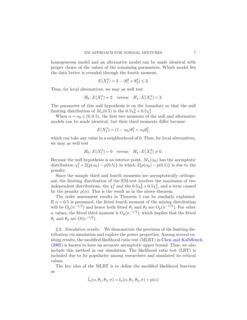
homogeneous model and an alternative model can be made identical withproper choice of the values of the remaining parameters. Which model fitsthe data better is revealed through the fourth moment,
E(X41 ) = 3− (θ4
1 + θ42) ≤ 3.
Thus, for local alternatives, we may as well test
H0 :E(X41 ) = 3 versus Ha :E(X4
1 ) < 3.
The parameter of this null hypothesis is on the boundary so that the nulllimiting distribution of Mn(0.5) is the 0.5χ2
0 + 0.5χ21.
When α = α0 ∈ (0,0.5), the first two moments of the null and alternativemodels can be made identical, but their third moments differ because
E(X31 ) = (1−α0)θ
31 + α0θ
32,
which can take any value in a neighborhood of 0. Thus, for local alternatives,we may as well test
H0 :E(X31 ) = 0 versus Ha :E(X3
1 ) 6= 0.
Because the null hypothesis is an interior point, Mn(α0) has the asymptoticdistribution χ2
1 + 2{p(α0)− p(0.5)} in which 2{p(α0)− p(0.5)} is due to thepenalty.
Since the sample third and fourth moments are asymptotically orthogo-nal, the limiting distribution of the EM-test involves the maximum of twoindependent distributions, the χ2
1 and the 0.5χ20 + 0.5χ2
1, and a term causedby the penalty p(α). This is the result as in the above theorem.
The order assessment results in Theorem 1 can be similarly explained.If α = 0.5 is presumed, the fitted fourth moment of the mixing distributionwill be Op(n
−1/2) and hence both fitted θ1 and θ2 are Op(n−1/8). For other
α values, the fitted third moment is Op(n−1/2), which implies that the fitted
θ1 and θ2 are O(n−1/6).
2.2. Simulation results. We demonstrate the precision of the limiting dis-tribution via simulation and explore the power properties. Among several ex-isting results, the modified likelihood ratio test (MLRT) in Chen and Kalbfleisch(2005) is known to have an accurate asymptotic upper bound. Thus, we alsoinclude this method in our simulation. The likelihood ratio test (LRT) isincluded due to its popularity among researchers and simulated its criticalvalues.
The key idea of the MLRT is to define the modified likelihood functionas
l̃n(α, θ1, θ2, σ) = ln(α, θ1, θ2, σ) + p(α)
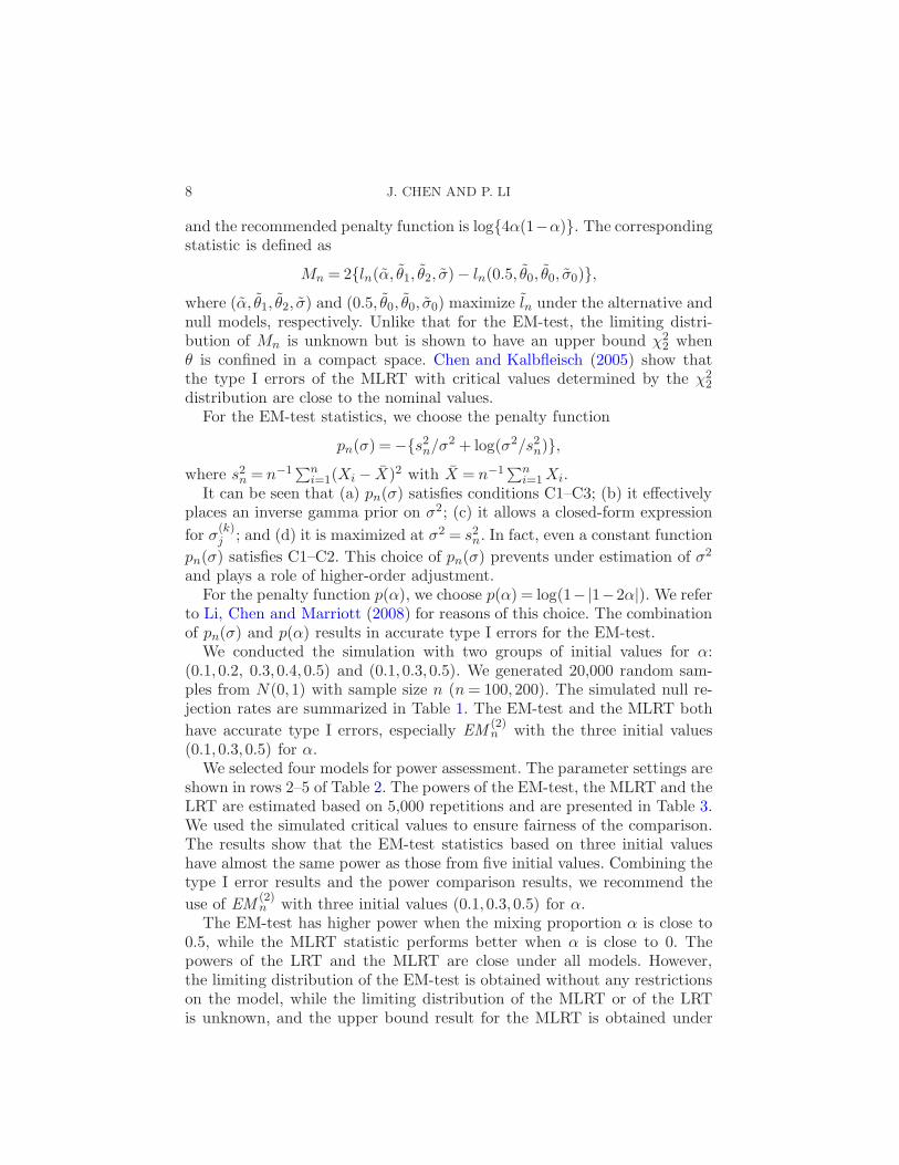
8 J. CHEN AND P. LI
and the recommended penalty function is log{4α(1−α)}. The correspondingstatistic is defined as
Mn = 2{ln(α̃, θ̃1, θ̃2, σ̃)− ln(0.5, θ̃0, θ̃0, σ̃0)},where (α̃, θ̃1, θ̃2, σ̃) and (0.5, θ̃0, θ̃0, σ̃0) maximize l̃n under the alternative andnull models, respectively. Unlike that for the EM-test, the limiting distri-bution of Mn is unknown but is shown to have an upper bound χ2
2 whenθ is confined in a compact space. Chen and Kalbfleisch (2005) show thatthe type I errors of the MLRT with critical values determined by the χ2
2
distribution are close to the nominal values.For the EM-test statistics, we choose the penalty function
pn(σ) = −{s2n/σ2 + log(σ2/s2
n)},where s2
n = n−1∑ni=1(Xi − X̄)2 with X̄ = n−1∑n
i=1 Xi.It can be seen that (a) pn(σ) satisfies conditions C1–C3; (b) it effectively
places an inverse gamma prior on σ2; (c) it allows a closed-form expression
for σ(k)j ; and (d) it is maximized at σ2 = s2
n. In fact, even a constant function
pn(σ) satisfies C1–C2. This choice of pn(σ) prevents under estimation of σ2
and plays a role of higher-order adjustment.For the penalty function p(α), we choose p(α) = log(1−|1−2α|). We refer
to Li, Chen and Marriott (2008) for reasons of this choice. The combinationof pn(σ) and p(α) results in accurate type I errors for the EM-test.
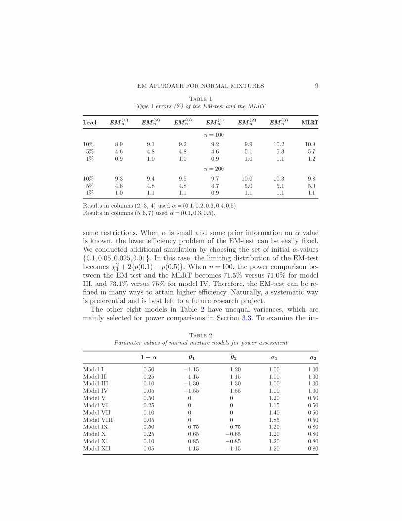
We conducted the simulation with two groups of initial values for α:(0.1,0.2, 0.3,0.4,0.5) and (0.1,0.3,0.5). We generated 20,000 random sam-ples from N(0,1) with sample size n (n = 100,200). The simulated null re-jection rates are summarized in Table 1. The EM-test and the MLRT both
have accurate type I errors, especially EM(2)n with the three initial values
(0.1,0.3,0.5) for α.We selected four models for power assessment. The parameter settings are
shown in rows 2–5 of Table 2. The powers of the EM-test, the MLRT and theLRT are estimated based on 5,000 repetitions and are presented in Table 3.We used the simulated critical values to ensure fairness of the comparison.The results show that the EM-test statistics based on three initial valueshave almost the same power as those from five initial values. Combining thetype I error results and the power comparison results, we recommend the
use of EM(2)n with three initial values (0.1,0.3,0.5) for α.
The EM-test has higher power when the mixing proportion α is close to0.5, while the MLRT statistic performs better when α is close to 0. Thepowers of the LRT and the MLRT are close under all models. However,the limiting distribution of the EM-test is obtained without any restrictionson the model, while the limiting distribution of the MLRT or of the LRTis unknown, and the upper bound result for the MLRT is obtained under
EM APPROACH FOR NORMAL MIXTURES 9
Table 1
Type I errors (%) of the EM-test and the MLRT
Level EM(1)n EM
(2)n EM
(3)n EM
(1)n EM
(2)n EM
(3)n MLRT
n = 100
10% 8.9 9.1 9.2 9.2 9.9 10.2 10.95% 4.6 4.8 4.8 4.6 5.1 5.3 5.71% 0.9 1.0 1.0 0.9 1.0 1.1 1.2
n = 200
10% 9.3 9.4 9.5 9.7 10.0 10.3 9.85% 4.6 4.8 4.8 4.7 5.0 5.1 5.01% 1.0 1.1 1.1 0.9 1.1 1.1 1.1
Results in columns (2, 3, 4) used α = (0.1,0.2,0.3,0.4,0.5).Results in columns (5,6,7) used α = (0.1,0.3,0.5).
some restrictions. When α is small and some prior information on α valueis known, the lower efficiency problem of the EM-test can be easily fixed.We conducted additional simulation by choosing the set of initial α-values{0.1,0.05,0.025,0.01}. In this case, the limiting distribution of the EM-testbecomes χ2
1 + 2{p(0.1) − p(0.5)}. When n = 100, the power comparison be-tween the EM-test and the MLRT becomes 71.5% versus 71.0% for modelIII, and 73.1% versus 75% for model IV. Therefore, the EM-test can be re-fined in many ways to attain higher efficiency. Naturally, a systematic wayis preferential and is best left to a future research project.
The other eight models in Table 2 have unequal variances, which aremainly selected for power comparisons in Section 3.3. To examine the im-
Table 2
Parameter values of normal mixture models for power assessment
1 − α θ1 θ2 σ1 σ2
Model I 0.50 −1.15 1.20 1.00 1.00Model II 0.25 −1.15 1.15 1.00 1.00Model III 0.10 −1.30 1.30 1.00 1.00Model IV 0.05 −1.55 1.55 1.00 1.00Model V 0.50 0 0 1.20 0.50Model VI 0.25 0 0 1.15 0.50Model VII 0.10 0 0 1.40 0.50Model VIII 0.05 0 0 1.85 0.50Model IX 0.50 0.75 −0.75 1.20 0.80Model X 0.25 0.65 −0.65 1.20 0.80Model XI 0.10 0.85 −0.85 1.20 0.80Model XII 0.05 1.15 −1.15 1.20 0.80
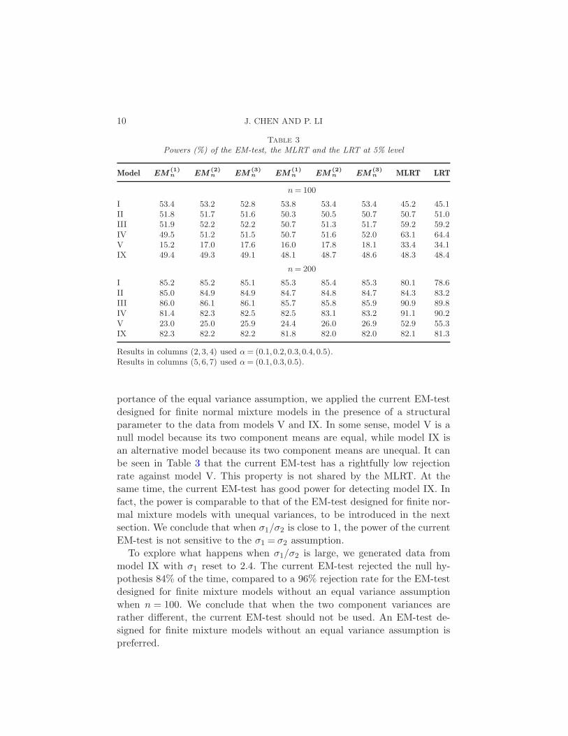
10 J. CHEN AND P. LI
Table 3
Powers (%) of the EM-test, the MLRT and the LRT at 5% level
Model EM(1)n EM
(2)n EM
(3)n EM
(1)n EM
(2)n EM
(3)n MLRT LRT
n = 100
I 53.4 53.2 52.8 53.8 53.4 53.4 45.2 45.1II 51.8 51.7 51.6 50.3 50.5 50.7 50.7 51.0III 51.9 52.2 52.2 50.7 51.3 51.7 59.2 59.2IV 49.5 51.2 51.5 50.7 51.6 52.0 63.1 64.4V 15.2 17.0 17.6 16.0 17.8 18.1 33.4 34.1IX 49.4 49.3 49.1 48.1 48.7 48.6 48.3 48.4
n = 200
I 85.2 85.2 85.1 85.3 85.4 85.3 80.1 78.6II 85.0 84.9 84.9 84.7 84.8 84.7 84.3 83.2III 86.0 86.1 86.1 85.7 85.8 85.9 90.9 89.8IV 81.4 82.3 82.5 82.5 83.1 83.2 91.1 90.2V 23.0 25.0 25.9 24.4 26.0 26.9 52.9 55.3IX 82.3 82.2 82.2 81.8 82.0 82.0 82.1 81.3
Results in columns (2,3,4) used α = (0.1,0.2,0.3,0.4,0.5).Results in columns (5,6,7) used α = (0.1,0.3,0.5).
portance of the equal variance assumption, we applied the current EM-test
designed for finite normal mixture models in the presence of a structural
parameter to the data from models V and IX. In some sense, model V is a
null model because its two component means are equal, while model IX is
an alternative model because its two component means are unequal. It can
be seen in Table 3 that the current EM-test has a rightfully low rejection
rate against model V. This property is not shared by the MLRT. At the
same time, the current EM-test has good power for detecting model IX. In
fact, the power is comparable to that of the EM-test designed for finite nor-
mal mixture models with unequal variances, to be introduced in the next
section. We conclude that when σ1/σ2 is close to 1, the power of the current
EM-test is not sensitive to the σ1 = σ2 assumption.
To explore what happens when σ1/σ2 is large, we generated data from
model IX with σ1 reset to 2.4. The current EM-test rejected the null hy-
pothesis 84% of the time, compared to a 96% rejection rate for the EM-test
designed for finite mixture models without an equal variance assumption
when n = 100. We conclude that when the two component variances are
rather different, the current EM-test should not be used. An EM-test de-
signed for finite mixture models without an equal variance assumption is
preferred.
EM APPROACH FOR NORMAL MIXTURES 11
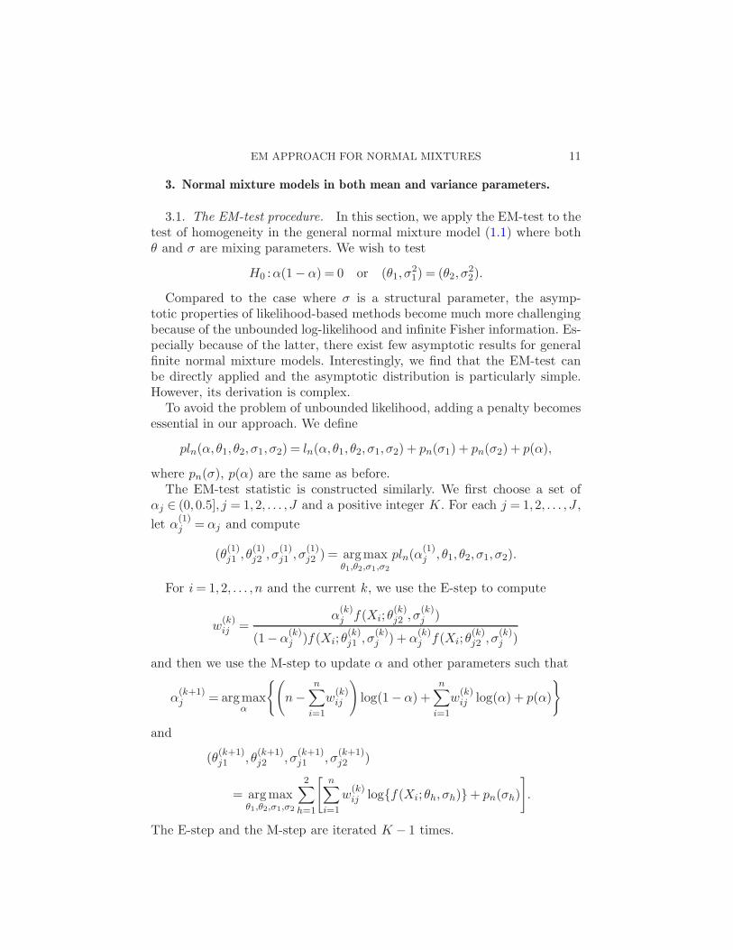
3. Normal mixture models in both mean and variance parameters.
3.1. The EM-test procedure. In this section, we apply the EM-test to thetest of homogeneity in the general normal mixture model (1.1) where bothθ and σ are mixing parameters. We wish to test
H0 :α(1− α) = 0 or (θ1, σ21) = (θ2, σ
22).
Compared to the case where σ is a structural parameter, the asymp-totic properties of likelihood-based methods become much more challengingbecause of the unbounded log-likelihood and infinite Fisher information. Es-pecially because of the latter, there exist few asymptotic results for generalfinite normal mixture models. Interestingly, we find that the EM-test canbe directly applied and the asymptotic distribution is particularly simple.However, its derivation is complex.
To avoid the problem of unbounded likelihood, adding a penalty becomesessential in our approach. We define
pln(α, θ1, θ2, σ1, σ2) = ln(α, θ1, θ2, σ1, σ2) + pn(σ1) + pn(σ2) + p(α),
where pn(σ), p(α) are the same as before.The EM-test statistic is constructed similarly. We first choose a set of
αj ∈ (0,0.5], j = 1,2, . . . , J and a positive integer K. For each j = 1,2, . . . , J ,
let α(1)j = αj and compute
(θ(1)j1 , θ
(1)j2 , σ
(1)j1 , σ
(1)j2 ) = argmax
θ1,θ2,σ1,σ2
pln(α(1)j , θ1, θ2, σ1, σ2).
For i = 1,2, . . . , n and the current k, we use the E-step to compute
w(k)ij =
α(k)j f(Xi;θ
(k)j2 , σ
(k)j )
(1−α(k)j )f(Xi;θ
(k)j1 , σ
(k)j ) + α
(k)j f(Xi;θ
(k)j2 , σ
(k)j )
and then we use the M-step to update α and other parameters such that
α(k+1)j = argmax
α
{(
n−n∑
i=1
w(k)ij
)
log(1−α) +n∑
i=1
w(k)ij log(α) + p(α)
}
and
(θ(k+1)j1 , θ
(k+1)j2 , σ
(k+1)j1 , σ
(k+1)j2 )
= argmaxθ1,θ2,σ1,σ2
2∑
h=1
[
n∑
i=1
w(k)ij log{f(Xi;θh, σh)}+ pn(σh)
]
.
The E-step and the M-step are iterated K − 1 times.
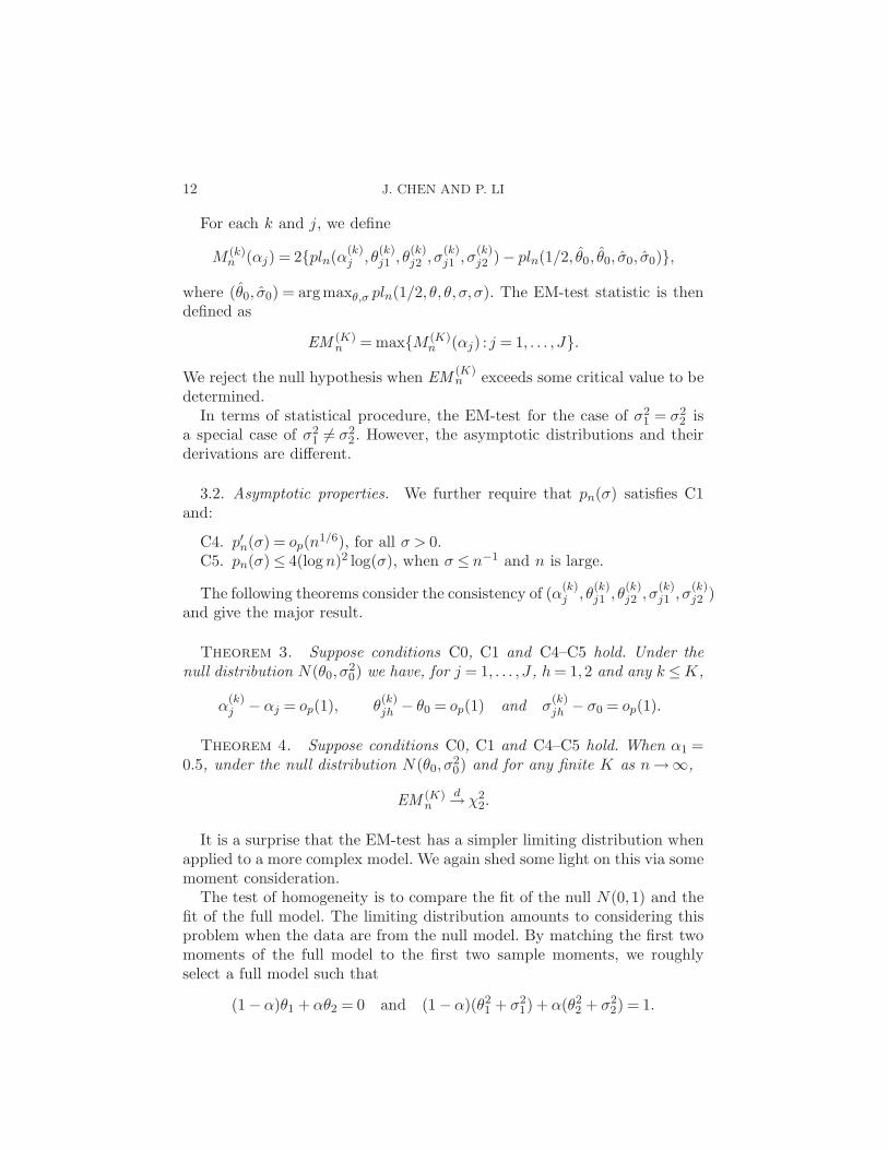
12 J. CHEN AND P. LI
For each k and j, we define
M (k)n (αj) = 2{pln(α
(k)j , θ
(k)j1 , θ
(k)j2 , σ
(k)j1 , σ
(k)j2 )− pln(1/2, θ̂0, θ̂0, σ̂0, σ̂0)},
where (θ̂0, σ̂0) = argmaxθ,σ pln(1/2, θ, θ, σ,σ). The EM-test statistic is thendefined as
EM (K)n = max{M (K)
n (αj) : j = 1, . . . , J}.
We reject the null hypothesis when EM(K)n exceeds some critical value to be
determined.In terms of statistical procedure, the EM-test for the case of σ2
1 = σ22 is
a special case of σ21 6= σ2
2 . However, the asymptotic distributions and theirderivations are different.
3.2. Asymptotic properties. We further require that pn(σ) satisfies C1and:
C4. p′n(σ) = op(n1/6), for all σ > 0.
C5. pn(σ) ≤ 4(log n)2 log(σ), when σ ≤ n−1 and n is large.
The following theorems consider the consistency of (α(k)j , θ
(k)j1 , θ
(k)j2 , σ
(k)j1 , σ
(k)j2 )
and give the major result.
Theorem 3. Suppose conditions C0, C1 and C4–C5 hold. Under the
null distribution N(θ0, σ20) we have, for j = 1, . . . , J , h = 1,2 and any k ≤ K,
α(k)j − αj = op(1), θ
(k)jh − θ0 = op(1) and σ
(k)jh − σ0 = op(1).
Theorem 4. Suppose conditions C0, C1 and C4–C5 hold. When α1 =0.5, under the null distribution N(θ0, σ
20) and for any finite K as n →∞,
EM (K)n
d→ χ22.
It is a surprise that the EM-test has a simpler limiting distribution whenapplied to a more complex model. We again shed some light on this via somemoment consideration.
The test of homogeneity is to compare the fit of the null N(0,1) and thefit of the full model. The limiting distribution amounts to considering thisproblem when the data are from the null model. By matching the first twomoments of the full model to the first two sample moments, we roughlyselect a full model such that
(1−α)θ1 + αθ2 = 0 and (1−α)(θ21 + σ2
1) + α(θ22 + σ2
2) = 1.
EM APPROACH FOR NORMAL MIXTURES 13
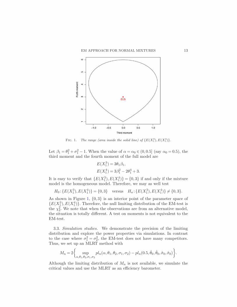
Fig. 1. The range (area inside the solid line) of {E(X31 ),E(X4
1 )}.
Let β1 = θ21 + σ2
1 − 1. When the value of α = α0 ∈ (0,0.5] (say α0 = 0.5), thethird moment and the fourth moment of the full model are
E(X31 ) = 3θ1β1,
E(X41 ) = 3β2
1 − 2θ41 + 3.
It is easy to verify that {E(X31 ),E(X4
1 )} = {0,3} if and only if the mixturemodel is the homogeneous model. Therefore, we may as well test
H0 :{E(X31 ),E(X4
1 )} = {0,3} versus Ha :{E(X31 ),E(X4
1 )} 6= {0,3}.As shown in Figure 1, {0,3} is an interior point of the parameter space of{E(X3
1 ),E(X41 )}. Therefore, the null limiting distribution of the EM-test is
the χ22. We note that when the observations are from an alternative model,
the situation is totally different. A test on moments is not equivalent to theEM-test.
3.3. Simulation studies. We demonstrate the precision of the limitingdistribution and explore the power properties via simulations. In contrastto the case where σ2
1 = σ22 , the EM-test does not have many competitors.
Thus, we set up an MLRT method with
Mn = 2
{
supα,θ1,θ2,σ1,σ2
pln(α, θ1, θ2, σ1, σ2)− pln(0.5, θ̂0, θ̂0, σ̂0, σ̂0)
}
.
Although the limiting distribution of Mn is not available, we simulate thecritical values and use the MLRT as an efficiency barometer.

14 J. CHEN AND P. LI
We suggest using the penalty function pn(σ) =−0.25{s2n/σ2+log(σ2/s2
n)},which is almost the same as before except for the coefficient because we havetwo penalty terms in this problem. Our simulation shows that this choiceworks well in terms of providing accurate type I errors. We use p(α) =log(1−|1−2α|) according to the recommendation of Li, Chen and Marriott(2008).
In the simulations, the type I errors were calculated based on 20,000samples from N(0,1). As in Section 2.2, we used two groups of initial val-
ues (0.1,0.2,0.3,0.4,0.5) and (0.1,0.3,0.5) to calculate EM(K)n . The simu-
lation results are summarized in Table 4. The EM-test statistics based on(0.1,0.3,0.5) give accurate type I errors.
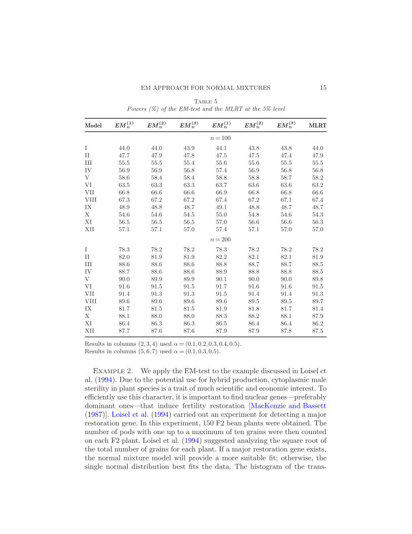
The powers of the EM-test and the MLRT for the models in Table 2 arecalculated based on 5,000 repetitions and presented in Table 5. Since thelimiting distribution of the MLRT is unavailable and hence is not a viablemethod, the simulated critical values were used for power calculation. The
simulation results show that the EM(2)n and EM
(3)n based on three initial
values (0.1,0.3,0.5) for α have almost the same power as the MLRT. Furtherincreasing the number of iterations or the number of initial values for α doesnot increase the power of the EM-test statistics. We therefore recommend
the use of EM(2)n or EM
(3)n based on three initial values (0.1,0.3,0.5) for α.
We note that when σ1 = σ2, the current EM-test loses some power com-pared to the EM-test designed for finite mixture models in the presence ofa structural parameter if the mixing parameter α is close to 0.5, but it hashigher power when α is near 0 or 1. Nevertheless, we recommend the use ofthe current EM-test if the equal variance assumption is likely violated.
4. Genetic applications.
Table 4
Type I errors (%) of the EM-test
Level EM(1)n EM
(2)n EM
(3)n EM
(1)n EM
(2)n EM
(3)n
n = 100
10% 10.8 10.9 10.9 10.5 10.6 10.65% 5.5 5.5 5.6 5.3 5.4 5.41% 1.2 1.2 1.2 1.1 1.2 1.2
n = 200
10% 10.7 10.7 10.7 10.4 10.5 10.55% 5.4 5.4 5.4 5.1 5.2 5.21% 1.1 1.1 1.1 1.0 1.0 1.0
Results in columns (2,3,4) used α = (0.1,0.2,0.3,0.4,0.5).Results in columns (5,6,7) used α = (0.1,0.3,0.5).
EM APPROACH FOR NORMAL MIXTURES 15
Table 5
Powers (%) of the EM-test and the MLRT at the 5% level
Model EM(1)n EM
(2)n EM
(3)n EM
(1)n EM
(2)n EM
(3)n MLRT
n = 100
I 44.0 44.0 43.9 44.1 43.8 43.8 44.0II 47.7 47.9 47.8 47.5 47.5 47.4 47.9III 55.5 55.5 55.4 55.6 55.6 55.5 55.5IV 56.9 56.9 56.8 57.4 56.9 56.8 56.8V 58.6 58.4 58.4 58.8 58.8 58.7 58.2VI 63.5 63.3 63.3 63.7 63.6 63.6 63.2VII 66.8 66.6 66.6 66.9 66.8 66.8 66.6VIII 67.3 67.2 67.2 67.4 67.2 67.1 67.4IX 48.9 48.8 48.7 49.1 48.8 48.7 48.7X 54.6 54.6 54.5 55.0 54.8 54.6 54.3XI 56.5 56.5 56.5 57.0 56.6 56.6 56.3XII 57.1 57.1 57.0 57.4 57.1 57.0 57.0
n = 200
I 78.3 78.2 78.2 78.3 78.2 78.2 78.2II 82.0 81.9 81.9 82.2 82.1 82.1 81.9III 88.6 88.6 88.6 88.8 88.7 88.7 88.5IV 88.7 88.6 88.6 88.9 88.8 88.8 88.5V 90.0 89.9 89.9 90.1 90.0 90.0 89.8VI 91.6 91.5 91.5 91.7 91.6 91.6 91.5VII 91.4 91.3 91.3 91.5 91.4 91.4 91.3VIII 89.6 89.6 89.6 89.6 89.5 89.5 89.7IX 81.7 81.5 81.5 81.9 81.8 81.7 81.4X 88.1 88.0 88.0 88.3 88.2 88.1 87.9XI 86.4 86.3 86.3 86.5 86.4 86.4 86.2XII 87.7 87.6 87.6 87.9 87.9 87.8 87.5
Results in columns (2,3,4) used α = (0.1,0.2,0.3,0.4,0.5).Results in columns (5,6,7) used α = (0.1,0.3,0.5).
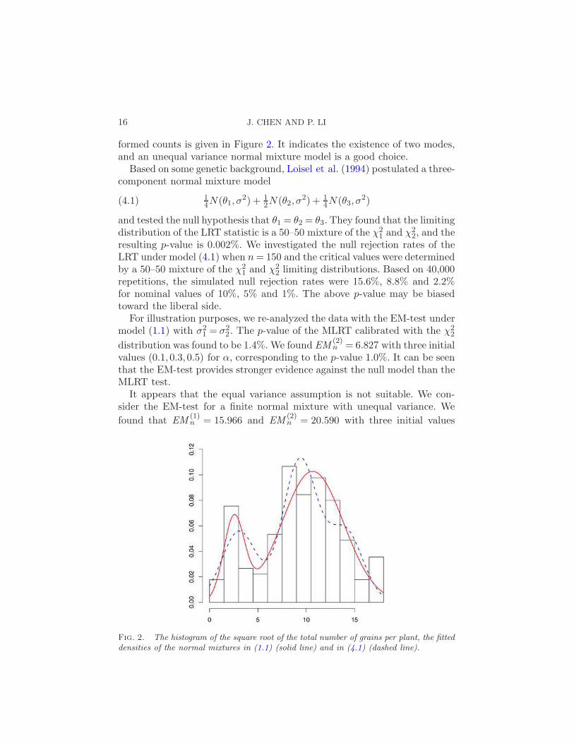
Example 2. We apply the EM-test to the example discussed in Loisel etal. (1994). Due to the potential use for hybrid production, cytoplasmic malesterility in plant species is a trait of much scientific and economic interest. Toefficiently use this character, it is important to find nuclear genes—preferablydominant ones—that induce fertility restoration [MacKenzie and Bassett(1987)]. Loisel et al. (1994) carried out an experiment for detecting a majorrestoration gene. In this experiment, 150 F2 bean plants were obtained. Thenumber of pods with one up to a maximum of ten grains were then countedon each F2 plant. Loisel et al. (1994) suggested analyzing the square root ofthe total number of grains for each plant. If a major restoration gene exists,the normal mixture model will provide a more suitable fit; otherwise, thesingle normal distribution best fits the data. The histogram of the trans-
16 J. CHEN AND P. LI
formed counts is given in Figure 2. It indicates the existence of two modes,and an unequal variance normal mixture model is a good choice.
Based on some genetic background, Loisel et al. (1994) postulated a three-component normal mixture model
14N(θ1, σ
2) + 12N(θ2, σ
2) + 14N(θ3, σ
2)(4.1)
and tested the null hypothesis that θ1 = θ2 = θ3. They found that the limitingdistribution of the LRT statistic is a 50–50 mixture of the χ2
1 and χ22, and the
resulting p-value is 0.002%. We investigated the null rejection rates of theLRT under model (4.1) when n = 150 and the critical values were determinedby a 50–50 mixture of the χ2
1 and χ22 limiting distributions. Based on 40,000
repetitions, the simulated null rejection rates were 15.6%, 8.8% and 2.2%for nominal values of 10%, 5% and 1%. The above p-value may be biasedtoward the liberal side.
For illustration purposes, we re-analyzed the data with the EM-test undermodel (1.1) with σ2
1 = σ22 . The p-value of the MLRT calibrated with the χ2
2
distribution was found to be 1.4%. We found EM(2)n = 6.827 with three initial
values (0.1,0.3,0.5) for α, corresponding to the p-value 1.0%. It can be seenthat the EM-test provides stronger evidence against the null model than theMLRT test.
It appears that the equal variance assumption is not suitable. We con-sider the EM-test for a finite normal mixture with unequal variance. We
found that EM(1)n = 15.966 and EM
(2)n = 20.590 with three initial values
Fig. 2. The histogram of the square root of the total number of grains per plant, the fitteddensities of the normal mixtures in (1.1) (solid line) and in (4.1) (dashed line).
EM APPROACH FOR NORMAL MIXTURES 17
(0.1,0.3,0.5) for α, resulting in the p-values 0.03% and 0.003%, respectively.Further iteration does not change the p-value much. This result is in line withthe outcome of Loisel et al. (1994). The modified MLES of (α, θ1, θ2, σ1, σ2)are (0.175,10.663,2.535,3.203,1.080), confirming that σ1 6= σ2 and explain-ing why the EM-test under the general model gives much stronger evidenceagainst the null model.
Figure 2 shows the fitted density functions of models (1.1) and (4.1). Ouranalysis indicates that a two-component mixture model can fit the data justas well as the model suggested by Loisel et al. (1994). The question of whichmodel is more appropriate is not the focus of this paper.
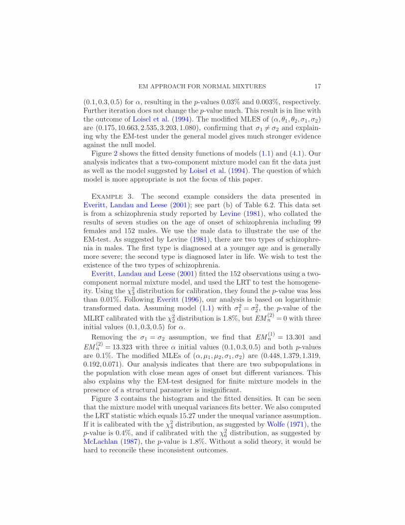
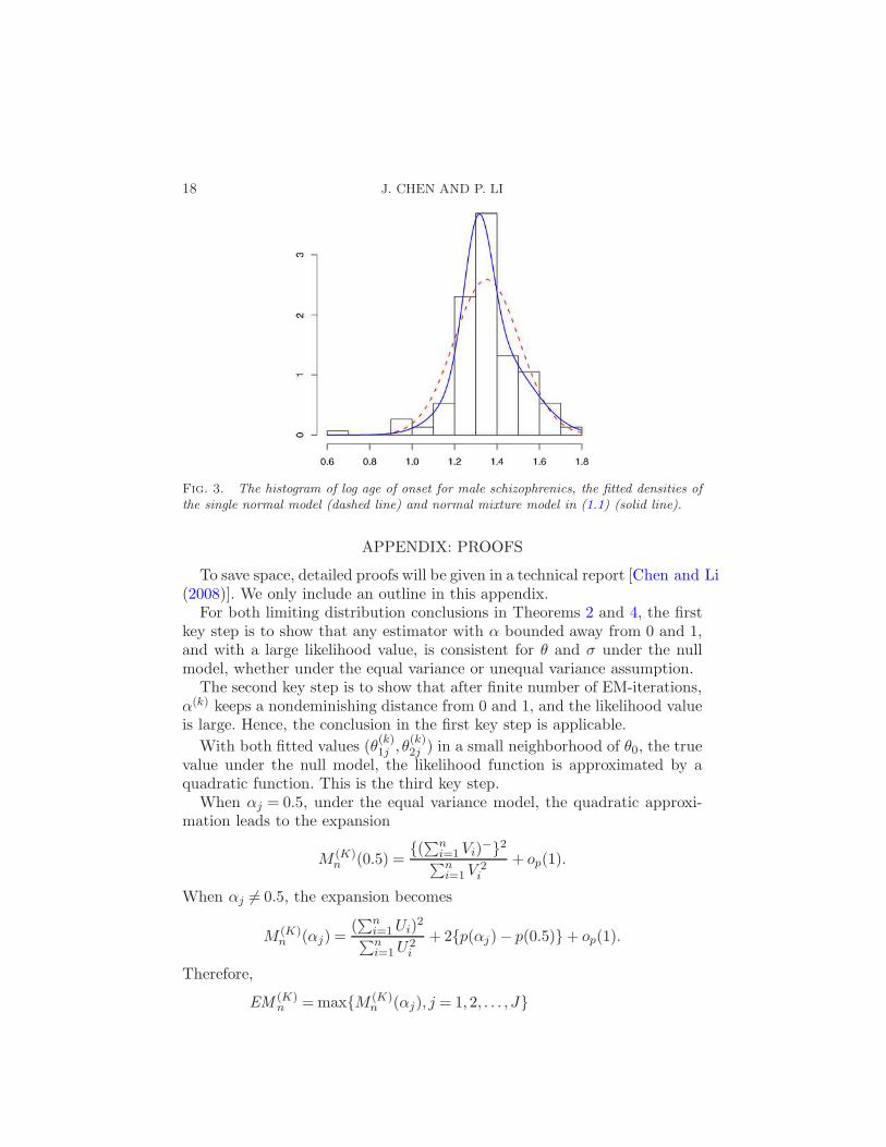
Example 3. The second example considers the data presented inEveritt, Landau and Leese (2001); see part (b) of Table 6.2. This data setis from a schizophrenia study reported by Levine (1981), who collated theresults of seven studies on the age of onset of schizophrenia including 99females and 152 males. We use the male data to illustrate the use of theEM-test. As suggested by Levine (1981), there are two types of schizophre-nia in males. The first type is diagnosed at a younger age and is generallymore severe; the second type is diagnosed later in life. We wish to test theexistence of the two types of schizophrenia.
Everitt, Landau and Leese (2001) fitted the 152 observations using a two-component normal mixture model, and used the LRT to test the homogene-ity. Using the χ2
3 distribution for calibration, they found the p-value was lessthan 0.01%. Following Everitt (1996), our analysis is based on logarithmictransformed data. Assuming model (1.1) with σ2
1 = σ22 , the p-value of the
MLRT calibrated with the χ22 distribution is 1.8%, but EM
(2)n = 0 with three
initial values (0.1,0.3,0.5) for α.
Removing the σ1 = σ2 assumption, we find that EM(1)n = 13.301 and
EM(2)n = 13.323 with three α initial values (0.1,0.3,0.5) and both p-values
are 0.1%. The modified MLEs of (α,µ1, µ2, σ1, σ2) are (0.448,1.379,1.319,0.192,0.071). Our analysis indicates that there are two subpopulations inthe population with close mean ages of onset but different variances. Thisalso explains why the EM-test designed for finite mixture models in thepresence of a structural parameter is insignificant.
Figure 3 contains the histogram and the fitted densities. It can be seenthat the mixture model with unequal variances fits better. We also computedthe LRT statistic which equals 15.27 under the unequal variance assumption.If it is calibrated with the χ2
4 distribution, as suggested by Wolfe (1971), thep-value is 0.4%, and if calibrated with the χ2
6 distribution, as suggested byMcLachlan (1987), the p-value is 1.8%. Without a solid theory, it would behard to reconcile these inconsistent outcomes.
18 J. CHEN AND P. LI
Fig. 3. The histogram of log age of onset for male schizophrenics, the fitted densities ofthe single normal model (dashed line) and normal mixture model in (1.1) (solid line).
APPENDIX: PROOFS
To save space, detailed proofs will be given in a technical report [Chen and Li(2008)]. We only include an outline in this appendix.
For both limiting distribution conclusions in Theorems 2 and 4, the firstkey step is to show that any estimator with α bounded away from 0 and 1,and with a large likelihood value, is consistent for θ and σ under the nullmodel, whether under the equal variance or unequal variance assumption.
The second key step is to show that after finite number of EM-iterations,α(k) keeps a nondeminishing distance from 0 and 1, and the likelihood valueis large. Hence, the conclusion in the first key step is applicable.
With both fitted values (θ(k)1j , θ
(k)2j ) in a small neighborhood of θ0, the true
value under the null model, the likelihood function is approximated by aquadratic function. This is the third key step.
When αj = 0.5, under the equal variance model, the quadratic approxi-mation leads to the expansion
M (K)n (0.5) =
{(∑ni=1 Vi)
−}2
∑ni=1 V 2
i
+ op(1).
When αj 6= 0.5, the expansion becomes
M (K)n (αj) =
(∑n
i=1 Ui)2
∑ni=1 U2
i
+ 2{p(αj)− p(0.5)} + op(1).
Therefore,
EM (K)n = max{M (K)
n (αj), j = 1,2, . . . , J}
EM APPROACH FOR NORMAL MIXTURES 19
= max
[
(∑n
i=1 Ui)2
∑ni=1 U2
i
+ ∆,{(∑n
i=1 Vi)−}2
∑ni=1 V 2
i
]
+ op(1).
We omit the definitions of Ui and Vi but point out that∑n
i=1 Ui/√
n and∑n
i=1 Vi/√
n are jointly asymptotical bivariate normal and independent. Con-
sequently, the limiting distribution of EM (K) is given by F (x − ∆){0.5 +0.5F (x)} with F (x) being the CDF of the χ2
1 distribution.Under the unequal variance assumption, the asymptotic expansion is
found to be
EM (K)n =
(∑n
i=1 Ui)2
∑ni=1U
2i
+(∑n
i=1 Vi)2
∑ni=1V
2i
+ op(1).
Consequently, the limiting distribution of EM(K)n is the χ2
2.
REFERENCES
Cai, T., Jin, J. and Low, M. (2007). Estimation and confidence sets for sparse normalmixtures. Ann. Statist. 35 2421–2449. MR2382653
Charnigo, R. and Sun, J. (2004). Testing homogeneity in a mixture distribution viathe L2-distance between competing models. J. Amer. Statist. Assoc. 99 488–498.MR2062834
Chen, H. and Chen, J. (2003). Tests for homogeneity in normal mixtures with presenceof a structural parameter. Statist. Sinica 13 351–365. MR1977730
Chen, H., Chen, J. and Kalbfleisch, J. D. (2001). A modified likelihood ratio forhomogeneity in finite mixture models. J. R. Stat. Soc. Ser. B Stat. Methodol. 63 19–29.MR1811988
Chen, J. (1995). Optimal rate of convergence in finite mixture models. Ann. Statist. 23
221–234. MR1331665Chen, J. and Kalbfleisch, J. D. (2005). Modified likelihood ratio test in finite mix-
ture models with a structural parameter. J. Statist. Plann. Inference 129 93–107.MR2126840
Chen, J. and Li, P. (2008). Homogeneity test in normal mixture models: The EM ap-proach. Technical report, Univ. British Columbia.
Chen, J., Tan, X. and Zhang, R. (2008). Inference for normal mixtures in mean andvariance. Statist. Sinica. 18 443–465.
Dacunha-Castelle, D. and Gassiat, E. (1999). Testing the order of a model usinglocally conic parametrization: Population mixtures and stationary ARMA processes.Ann. Statist. 27 1178–1209. MR1740115
Efron, B. (2004). Large-scale simulation hypothesis testing: The choice of a null hypoth-esis. J. Amer. Statist. Assoc. 99 96–104. MR2054289
Everitt, B. S. (1996). An introduction to finite mixture distributions. Statist. MethodsMed. Research 5 107–127.
Everitt, B. S., Landau, S. and Leese, M. (2001). Cluster Analysis, 4th ed. OxfordUniv. Press, New York, NY. MR1217964
Feng, Z. D. and McCulloch, C. E. (1994). On the likelihood ratio test statistic forthe number of components in a normal mixture with unequal variances. Biometrics 50
1158–1162.Garel, B. (2005). Asymptotic theory of the likelihood ratio test for the identification of
a mixture. J. Statist. Plann. Inference 131 271–296. MR2139373
20 J. CHEN AND P. LI
Ghosh, J. K. and Sen, P. K. (1985). On the asymptotic performance of the log-likelihood
ratio statistic for the mixture model and related results. In Proceedings of the Berkeley
Conference in Honor of Jerzy Neyman and Jack Kiefer (L. LeCam and R. A. Olshen,
eds.) 2 789–806. Wadsworth, Monterey, CA. MR0822065
Hall, P. and Stewart, M. (2005). Theoretical analysis of power in a two-component
normal mixture model. J. Statist. Plann. Inference 134 158–179. MR2146091
Hartigan, J. A. (1985). A failure of likelihood asymptotics for normal mixtures. In
Proceedings of the Berkeley Conference in Honor of Jerzy Neyman and Jack Kiefer (L.
LeCam and R. A. Olshen, eds.) 2 807–810. Wadsworth, Monterey, CA. MR0822066
Hathaway, R. J. (1985). A constrained formulation of maximum-likelihood estimation
for normal mixture distributions. Ann. Statist. 13 795–800. MR0790575
Kon, S. (1984). Models of stock returns—A comparison. J. Finance 39 147–165.
Levine, R. (1981). Sex differences in schizophrenia: Timing or subtypes? Psychological
Bulletin 90 432–444.
Li, P., Chen, J. and Marriott, P. (2008). Nonfinite Fisher information and homogene-
ity: The EM approach. Biometrika. In press.
Liu, X., Pasarica, C. and Shao, Y. (2003). Testing homogeneity in gamma mixture
models. Scand. J. Statist. 30 227–239. MR1965104
Liu, X. and Shao, Y. Z. (2004). Asymptotics for likelihood ratio tests under loss of
identifiability. Ann. Statist. 31 807–832. MR1994731
Liu, X. and Shao, Y. Z. (2004). Asymptotics for the likelihood ratio test in a two-
component normal mixture model. J. Statist. Plann. Inference 123 61–81. MR2058122
Loisel, P., Goffinet, B., Monod, H. and Montes De Oca, G. (1994). Detecting a
major gene in an F2 population. Biometrics 50 512–516. MR1294684
MacKenzie, S. A. and Bassett, M. J. (1987). Genetics of fertility restoration in cy-
toplasmic sterile Phaseolus vulgaris L. I. Cytoplasmic alteration by a nuclear restorer
gene. Theoretical and Applied Genetics 74 642–645.
Marriott, P. (2007). Extending local mixture models. Ann. Inst. Statist. Math. 59 95–
110. MR2405288
McLachlan, G. J. (1987). On bootstrapping the likelihood ratio test statistic for the
number of components in a normal mixture. Applied Statistics 36 318–324.
McLachlan, G. J., Bean, R. W. and Ben-Tovim Jones, L. (2006). A simple imple-
mentation of a normal mixture approach to differential gene expression in multiclass
microarrays. Bioinformatics 22 1608–1615.
McLaren, C. E. (1996). Mixture models in haematology: A series of case studies. Stat.
Methods Med. Res. 5 129–153.
Pearson, K. (1894). Contributions to the mathematical theory of evolution. Philosophical
Transactions of the Royal Society of London A 185 71–110.
Raftery, A. E. and Dean, N. (2006). Variable selection for model-based clustering. J.
Amer. Statist. Assoc. 101 168–178. MR2268036
Roeder, K. (1994). A graphical technique for determining the number of components in
a mixture of normals. J. Amer. Statist. Assoc. 89 487–495. MR1294074
Schork, N. J., Allison, D. B. and Thiel, B. (1996). Mixture distributions in human
genetics research. Stat. Methods Med. Res. 5 155–178.
Sun, W. and Cai, T. T. (2007). Oracle and adaptive compound decision rules for false
discovery rate control. J. Amer. Statist. Assoc. 102 901–912. MR2411657
Tadesse, M., Sha, N. and Vannucci, M. (2005). Bayesian variable selection in clustering
high-dimensional data. J. Amer. Statist. Assoc. 100 602–617. MR2160563

EM APPROACH FOR NORMAL MIXTURES 21
Wolfe, J. H. (1971). A Monte Carlo study of the sampling distribution of the likelihoodratio for mixtures of multinormal distributions. Technical Bulletin STB 72-2, NavalPersonnel and Training Research Laboratory, San Diego.
Department of Statistics
University of British Columbia
Vancouver
British Columbia, V6T 1Z2
Canada
E-mail: [email protected]
Department of Mathematical
and Statistical Sciences
University of Alberta
Edmonton
T6G 2G1
Canada
E-mail: [email protected]