Ideal Hash Trees

Phil Bagwell

Hash Trees with nearly ideal characteristics are described. These Hash Trees require no initialroot hash table yet are faster and use significantly less space than chained or double hash trees.Insert, search and delete times are small and constant, independent of key set size, operations areO(1). Small worst-case times for insert, search and removal operations can be guaranteed andmisses cost less than successful searches. Array Mapped Tries(AMT), first described in Fast andSpace Efficient Trie Searches, Bagwell [2000], form the underlying data structure. The concept isthen applied to external disk or distributed storage to obtain an algorithm that achieves singleaccess searches, close to single access inserts and greater than 80 percent disk block load factors.Comparisons are made with Linear Hashing, Litwin, Neimat, and Schneider [1993] and B-Trees,R.Bayer and E.M.McCreight [1972]. In addition two further applications of AMTs are brieflydescribed, namely, Class/Selector dispatch tables and IP Routing tables. Each of the algorithmshas a performance and space usage that is comparable to contemporary implementations butsimpler.

Categories and Subject Descriptors: H.4.m [Information Systems]: Miscellaneous

General Terms: Hashing,Hash Tables,Row Displacement,Searching,Database,Routing,Routers

1. INTRODUCTION

The Hash Array Mapped Trie (HAMT) is based on the simple notion of hashinga key and storing the key in a trie based on this hash value. The AMT is usedto implement the required structure efficiently. The Array Mapped Trie (AMT) isa versatile data structure and yields attractive alternative to contemporary algo-rithms in many applications. Here I describe how it is used to develop Hash Treeswith near ideal characteristics that avoid the traditional problem, setting the size ofthe initial root hash table or incurring the high cost of dynamic resizing to achievean acceptable performance. Tries were first developed by Fredkin [1960] recentlyimplemented elegantly by Bentley and Sedgewick [1997] as the Ternary SearchTrees(TST), and by Nilsson and Tikkanen [1998] as Level Path Compressed(LPC)tries. AMT performs 3-4 times faster than TST using 60 percent less space and arefaster than LPC tries.

During a search bits are progressively used from the hash to traverse the trie untila key/value pair is found. During insert the AMT levels are extended using morehash bits until a new hash is differentiated from previously stored ones. It will beshown that the methods for Insert, Search and Delete are fast and independent ofkey set size. All these may be realized yet still guarantee that worst case operationtimes are no more than a few times the average case.

Linear Hash (LH), Litwin, Neimat, and Schneider [1993] derived from DynamicHash Tables, Larson [1988] offer an effective solution to collision management and

Address: Es Grands Champs, 1195-Dully, Switzerland

1

2 · Phil Bagwell

external storage growth by maintaining blocks with an acceptable load factor andsplitting on collisions. The underlying principle of HAMT, partitioning using ahash, has been developed and combined with the conceptual foundations of LH togive an algorithm that has better performance. The new Partition Hashing(PH)algorithm splits buckets evenly by the number of records and uses adjacent bucketsharing to improve load factor. A hash partition value is maintained for each bucketthat guides inserts and searches to the correct bucket. This results in a single accesssearch, inserts costing less than 1.1 accesses for a load factor exceeding 80 percent.If load factor is more critical than insert times for a given application the algorithmcan be optimized to give a load factor up to 100 percent with increased accessesper insert.

Adapting the algorithm to distributed processing is discussed briefly. The con-ceptual framework being adapted from LH*.

Further examples of the utility of AMT are covered in the section giving briefoverview of their application to Class/Selector dispatch tables, and IP Routingtables.

First I start with a brief summary of the AMT data structure before covering theHAMT and PH in more detail. Performance comparisons are included by section.

A more detailed description of the benchmark method can be found at the endof the paper.

2. ESSENTIALS OF THE ARRAY MAPPED TRIE

It should be noted that all the algorithms that follow have been optimized for a 32bit architecture and hence the AMT implementation has a natural cardinality of32. However it is a trivial matter to adapt the basic AMT to a 64 bit architecture.AMT’s for other alphabet cardinalities are covered in the paper, Fast and SpaceEfficient Trie Searches Bagwell [2000].

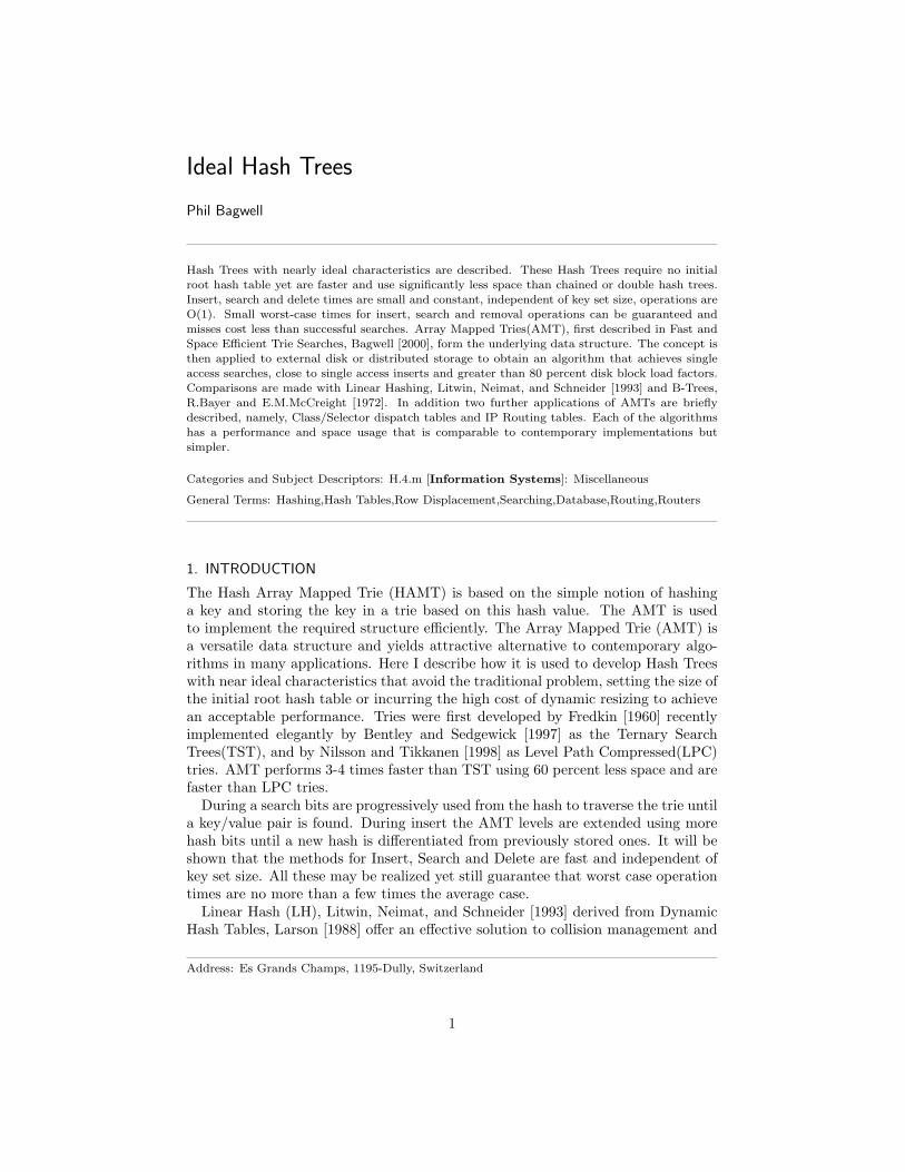
A trie is represented by a node and number of arcs leading to sub-tries and eacharc represents a member of an alphabet of possible alternatives. Here, to matchthe natural structure of a 32 bit system architecture, the alphabet is restricted toa cardinality 32 limiting the arcs to the range 0 to 31. The central dilemma inrepresenting such tries is to strike an acceptable balance between the desire for fasttraversal speed and minimizing the space lost for empty arcs.

The AMT data structure uses just two 32 bit words per node for a good compro-mise, achieving fast traversal at a cost of only one bit per empty arc. An integer bitmap is used to represent the existence of each of the 32 possible arcs and an associ-ated table contains pointers to the appropriate sub-tries or terminal nodes. A onebit in the bit map represents a valid arc, while a zero an empty arc. The pointersin the table are kept in sorted order and correspond to the order of each one bit inthe bit map. The tree is depicted in Fig 1. Note that map entries correspond tothe non-empty table entries of the next level down sub-trie.

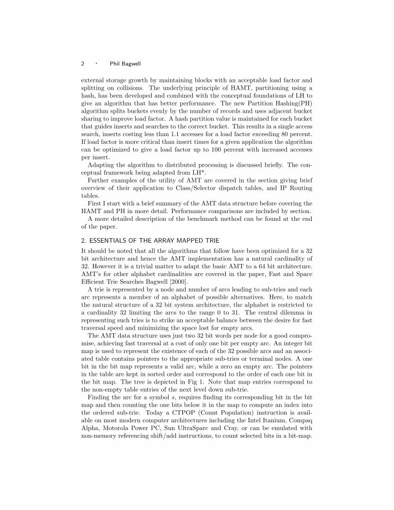
Finding the arc for a symbol s, requires finding its corresponding bit in the bitmap and then counting the one bits below it in the map to compute an index intothe ordered sub-trie. Today a CTPOP (Count Population) instruction is avail-able on most modern computer architectures including the Intel Itanium, CompaqAlpha, Motorola Power PC, Sun UltraSparc and Cray, or can be emulated withnon-memory referencing shift/add instructions, to count selected bits in a bit-map.

Ideal Hash Trees With AMT’s · 3

-Map SubTrie Map SubTrieMap SubTrieMap SubTrieMap SubTrie

Fig. 1. Array Mapped Trie

const unsigned int SK5=0x55555555,SK3=0x33333333;const unsigned int SKF0=0xF0F0F0F,SKFF=0xFF00FF;

int CTPop(int Map){Map-=((Map>>1)&SK5);Map=(Map&SK3)+((Map>>2)&SK3);Map=(Map&SKF0)+((Map>>4)&SKF0);Map+=Map>>8;return (Map+(Map>>16))&0x3F;}

Fig. 2. Emulation of CTPOP

3. IDEAL HASHING

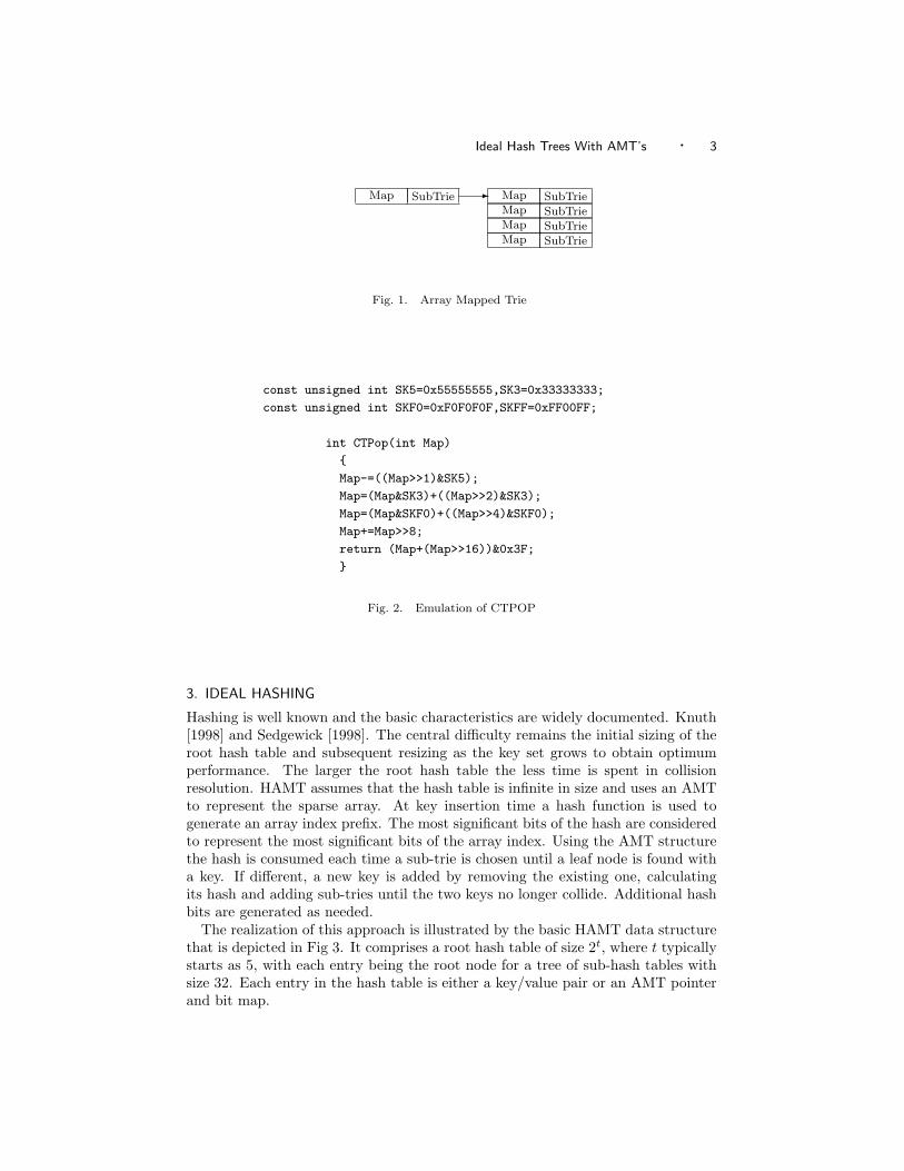
Hashing is well known and the basic characteristics are widely documented. Knuth[1998] and Sedgewick [1998]. The central difficulty remains the initial sizing of theroot hash table and subsequent resizing as the key set grows to obtain optimumperformance. The larger the root hash table the less time is spent in collisionresolution. HAMT assumes that the hash table is infinite in size and uses an AMTto represent the sparse array. At key insertion time a hash function is used togenerate an array index prefix. The most significant bits of the hash are consideredto represent the most significant bits of the array index. Using the AMT structurethe hash is consumed each time a sub-trie is chosen until a leaf node is found witha key. If different, a new key is added by removing the existing one, calculatingits hash and adding sub-tries until the two keys no longer collide. Additional hashbits are generated as needed.

The realization of this approach is illustrated by the basic HAMT data structurethat is depicted in Fig 3. It comprises a root hash table of size 2t, where t typicallystarts as 5, with each entry being the root node for a tree of sub-hash tables withsize 32. Each entry in the hash table is either a key/value pair or an AMT pointerand bit map.

4 · Phil Bagwell

Root Hash Table

-

Map BaseKey ValueMap BaseKey ValueMap Base -

Sub-Hash TableKey ValueMap BaseMap BaseMap Base

Sub-Hash TableKey ValueKey Value

Fig. 3. Hash Array Mapped Trie (HAMT)

3.1 Search for a key

Compute a full 32 bit hash for the key, take the most significant t bits and usethem as an integer to index into the root hash table. One of three cases may beencountered. First, the entry is empty indicating that the key is not in the hashtree. Second the entry is a Key/Value pair and the key either matches the desiredkey indicating success or not, indicating failure. Third, the entry has a 32 bit mapsub-hash table and a sub-trie pointer, Base, that points to an ordered list of thenon-empty sub-hash table entries.

Take the next 5 bits of the hash and use them as an integer to index into the bitMap. If this bit is a zero the hash table entry is empty indicating failure, otherwise,it’s a one, so count the one bits below it using CTPOP and use the result as theindex into the non-empty entry list at Base. This process is repeated taking fivemore bits of the hash each time until a terminating key/value pair is found or thesearch fails. Typically, only a few iterations are required and it is important tonote that the key is only compared once and that is with the terminating nodekey. This contributes significantly to the speed of the search since many memoryaccesses are avoided. Notice too that misses are detected early and rarely requirea key comparison.

Unlike Dynamic Perfect Hashing Dietzfelbinger, Karlin, Mehlhorn, auf der Heide,Rohnert, and Tarjan [1994]no effort is taken to minimize the size of the sub-hashtables. Instead the AMT data structure has been used to minimize the cost ofempty table entries. As the tree grows there is a small but increasing probabilitythat the number of iterations will cause the 32 bits in the hash to be exhausted anda new one must be computed. This is covered further in the following descriptionof the insertion algorithm.

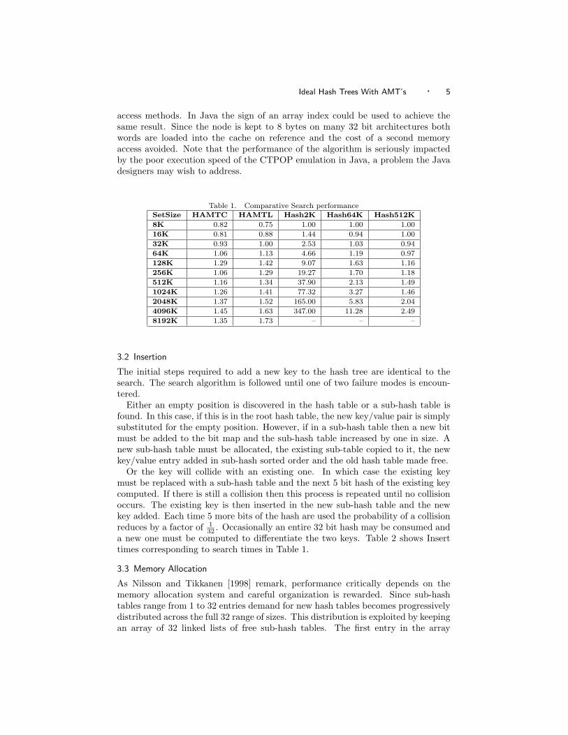
Assuming that the hash function generates a random distribution of keys thenon average the key hash will uniquely define a terminal node after lgN bits. Withan AMT 5 bits of the hash are taken at each iteration giving a search cost of 1

5 lgNor O(lgN). As will be shown later this can be reduced to an O(1) cost. Table 1shows search times for HAMTC with O(1) cost, HAMTL with O(lgN) and then achained hash tree with a root hash table of 2000, 64000 and 512000 entries. (Thebenchmark system memory capacity limited the Hash tests to 4096000 keys.)

A small, but important implementation consideration is the identification of sub-tries or key/value nodes by a bit flag in the data structure. Using C++ the bituses the least significant bit of the pointer and encapsulates this within the pointer

Ideal Hash Trees With AMT’s · 5

access methods. In Java the sign of an array index could be used to achieve thesame result. Since the node is kept to 8 bytes on many 32 bit architectures bothwords are loaded into the cache on reference and the cost of a second memoryaccess avoided. Note that the performance of the algorithm is seriously impactedby the poor execution speed of the CTPOP emulation in Java, a problem the Javadesigners may wish to address.

Table 1. Comparative Search performanceSetSize HAMTC HAMTL Hash2K Hash64K Hash512K8K 0.82 0.75 1.00 1.00 1.0016K 0.81 0.88 1.44 0.94 1.0032K 0.93 1.00 2.53 1.03 0.9464K 1.06 1.13 4.66 1.19 0.97128K 1.29 1.42 9.07 1.63 1.16256K 1.06 1.29 19.27 1.70 1.18512K 1.16 1.34 37.90 2.13 1.491024K 1.26 1.41 77.32 3.27 1.462048K 1.37 1.52 165.00 5.83 2.044096K 1.45 1.63 347.00 11.28 2.498192K 1.35 1.73 – – –

3.2 Insertion

The initial steps required to add a new key to the hash tree are identical to thesearch. The search algorithm is followed until one of two failure modes is encoun-tered.

Either an empty position is discovered in the hash table or a sub-hash table isfound. In this case, if this is in the root hash table, the new key/value pair is simplysubstituted for the empty position. However, if in a sub-hash table then a new bitmust be added to the bit map and the sub-hash table increased by one in size. Anew sub-hash table must be allocated, the existing sub-table copied to it, the newkey/value entry added in sub-hash sorted order and the old hash table made free.

Or the key will collide with an existing one. In which case the existing keymust be replaced with a sub-hash table and the next 5 bit hash of the existing keycomputed. If there is still a collision then this process is repeated until no collisionoccurs. The existing key is then inserted in the new sub-hash table and the newkey added. Each time 5 more bits of the hash are used the probability of a collisionreduces by a factor of 1

32 . Occasionally an entire 32 bit hash may be consumed anda new one must be computed to differentiate the two keys. Table 2 shows Inserttimes corresponding to search times in Table 1.

3.3 Memory Allocation

As Nilsson and Tikkanen [1998] remark, performance critically depends on thememory allocation system and careful organization is rewarded. Since sub-hashtables range from 1 to 32 entries demand for new hash tables becomes progressivelydistributed across the full 32 range of sizes. This distribution is exploited by keepingan array of 32 linked lists of free sub-hash tables. The first entry in the array

6 · Phil Bagwell

Table 2. Comparative Insert performanceSetSize HAMTC HAMTL Hash2 Hash64 Hash5128K 3.55 3.56 3.00 3.38 2.7516K 3.58 3.54 3.44 2.75 2.8132K 3.83 3.78 4.56 3.16 2.9764K 4.06 4.01 6.80 3.27 2.86128K 3.92 3.90 11.42 3.38 2.95256K 4.10 3.93 21.08 3.99 3.31512K 4.31 4.18 40.96 4.44 3.621024K 4.72 4.63 80.55 5.46 3.442048K 4.94 4.95 175.00 7.83 3.824096K 4.87 5.00 343.00 13.31 4.518192K 5.22 5.37 – – –

contains the list of all free sub-hash tables of length one, the second the list of all sub-hash tables of length two and so on. Thus allocating a new sub-hash table requiresthe minimum of work, either remove one from the appropriate free list or allocatea new one from free memory pool. The memory pool is allocated from systemmemory in blocks. A freed sub-hash table is simply attached to the appropriatefree list.

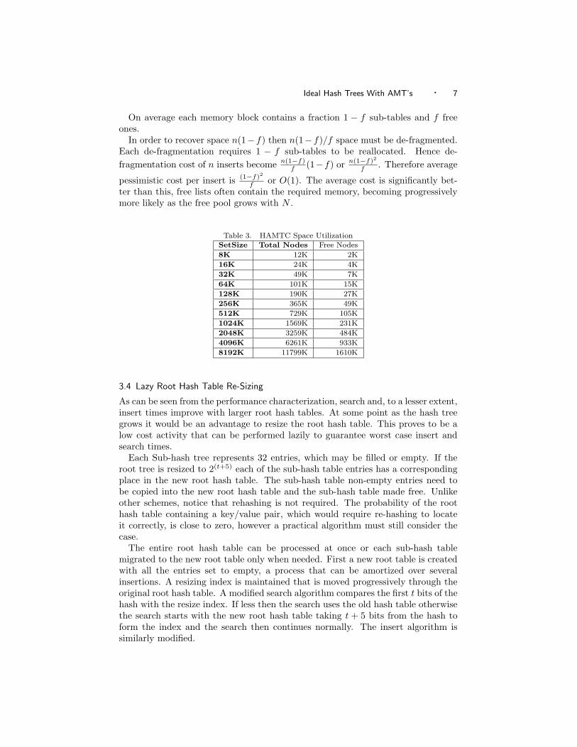
Clearly the distribution is not quite perfectly balanced, as the key set grows moresmall sub-hash trees are freed than are required later. Unchecked this leads to aset of free lists that are typically 3 times the used space, however with a littleingenuity memory pool blocks can be de-fragmented to recover the lost free space.A de-fragmentation threshold is set as a percentage of waste free memory allowed.If this is exceeded a memory pool block will be de-fragmented during the nextkey insertion. With this modification, space wasted is restricted to a few percentwith minor impact on insertion times. Table 3 shows total node usage, includingfree and the amount free, but excluding key string storage, with a threshold of 15percent. The variance in node consumption is also small when compared across alarge number of key sets.

The pool block size partially determines the time for insert or removal. In generalthe larger the pool blocks the better the amortized insertion time however blocksbeyond 2000 nodes give marginal improvement. When a pool block is de-fragmentedall the allocated sub-hash tables must be moved. Although not a costly activity itcould represent many insert times in the worst case. However, the de-fragmentationcan be carried out progressively, moving only one sub-hash table at each insert untilthe complete block is de-fragmented. With this modification the worst case becomesa few average insert times.

A pessimistic average de-fragmentation cost can be shown to be O(1). Supposethe free space ratio is set to a fraction f of the total space used S and a further nkeys are added. Note f=0.15 implies that 15% space is reserved in the linked freelists.

When a key is added a sub-table is freed with e entries, placed on the appropriatefree list and a new one is required with e + 1 entries. Hence after n inserts n sub-tables are freed and n new ones required. In order to keep the free space a constantthe de-fragmentation must recover worst case n(1 − f) trie nodes if they are notavailable on free lists in the required size.

Ideal Hash Trees With AMT’s · 7

On average each memory block contains a fraction 1 − f sub-tables and f freeones.

In order to recover space n(1− f) then n(1− f)/f space must be de-fragmented.Each de-fragmentation requires 1 − f sub-tables to be reallocated. Hence de-fragmentation cost of n inserts become n(1−f)

f (1−f) or n(1−f)2

f . Therefore average

pessimistic cost per insert is (1−f)2

f or O(1). The average cost is significantly bet-ter than this, free lists often contain the required memory, becoming progressivelymore likely as the free pool grows with N .

Table 3. HAMTC Space UtilizationSetSize Total Nodes Free Nodes8K 12K 2K16K 24K 4K32K 49K 7K64K 101K 15K128K 190K 27K256K 365K 49K512K 729K 105K1024K 1569K 231K2048K 3259K 484K4096K 6261K 933K8192K 11799K 1610K

3.4 Lazy Root Hash Table Re-Sizing

As can be seen from the performance characterization, search and, to a lesser extent,insert times improve with larger root hash tables. At some point as the hash treegrows it would be an advantage to resize the root hash table. This proves to be alow cost activity that can be performed lazily to guarantee worst case insert andsearch times.

Each Sub-hash tree represents 32 entries, which may be filled or empty. If theroot tree is resized to 2(t+5) each of the sub-hash table entries has a correspondingplace in the new root hash table. The sub-hash table non-empty entries need tobe copied into the new root hash table and the sub-hash table made free. Unlikeother schemes, notice that rehashing is not required. The probability of the roothash table containing a key/value pair, which would require re-hashing to locateit correctly, is close to zero, however a practical algorithm must still consider thecase.

The entire root hash table can be processed at once or each sub-hash tablemigrated to the new root table only when needed. First a new root table is createdwith all the entries set to empty, a process that can be amortized over severalinsertions. A resizing index is maintained that is moved progressively through theoriginal root hash table. A modified search algorithm compares the first t bits of thehash with the resize index. If less then the search uses the old hash table otherwisethe search starts with the new root hash table taking t + 5 bits from the hash toform the index and the search then continues normally. The insert algorithm issimilarly modified.

8 · Phil Bagwell

The hash table should be resized when the new hash table represents a reasonablefraction, say, 1

f of the total allocated space. This means that the first 15 lg N

f accesseswill be replaced by a single access in the hash table. Hence the average search andinsert costs become 1

5 lgN − 15 lg(N

f ) or 15 (lgf), i.e. O(1). Note, table resizing will

only occur when the new table is 32 times the size of the old one or when theoriginal table is 1

32f in size. It is sufficient therefore to move entries from the old to

the new root table once every, say, 32f2 inserts to complete this process before the

next resize could be required. Since one root table entry move is equivalent to afew average insert times this becomes the worse case insert time. All the HAMTCtimes in Table 1 and 2 result from using this lazy resizing algorithm.

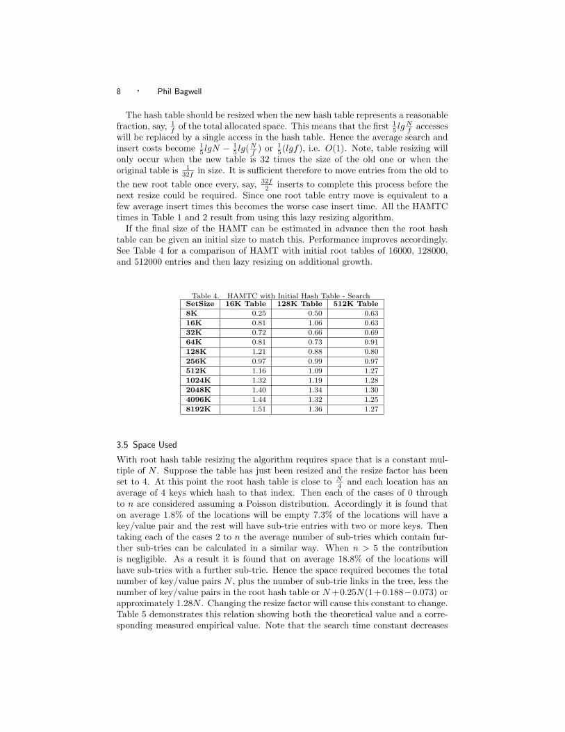
If the final size of the HAMT can be estimated in advance then the root hashtable can be given an initial size to match this. Performance improves accordingly.See Table 4 for a comparison of HAMT with initial root tables of 16000, 128000,and 512000 entries and then lazy resizing on additional growth.

Table 4. HAMTC with Initial Hash Table - SearchSetSize 16K Table 128K Table 512K Table8K 0.25 0.50 0.6316K 0.81 1.06 0.6332K 0.72 0.66 0.6964K 0.81 0.73 0.91128K 1.21 0.88 0.80256K 0.97 0.99 0.97512K 1.16 1.09 1.271024K 1.32 1.19 1.282048K 1.40 1.34 1.304096K 1.44 1.32 1.258192K 1.51 1.36 1.27

3.5 Space Used

With root hash table resizing the algorithm requires space that is a constant mul-tiple of N . Suppose the table has just been resized and the resize factor has beenset to 4. At this point the root hash table is close to N

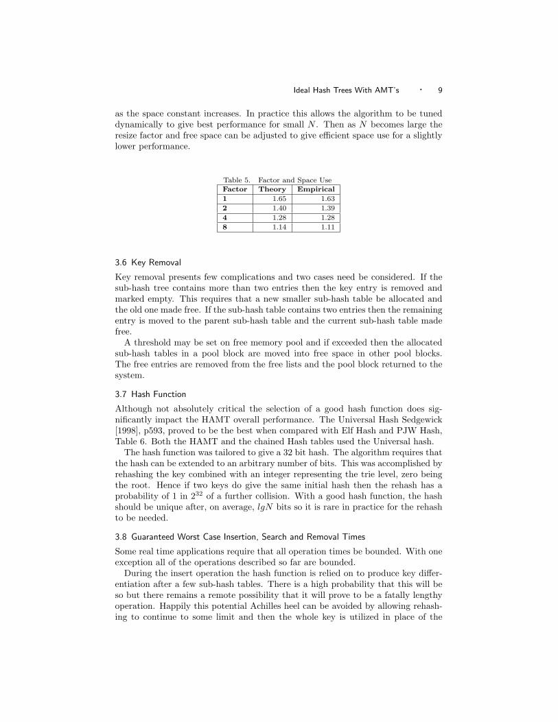
4 and each location has anaverage of 4 keys which hash to that index. Then each of the cases of 0 throughto n are considered assuming a Poisson distribution. Accordingly it is found thaton average 1.8% of the locations will be empty 7.3% of the locations will have akey/value pair and the rest will have sub-trie entries with two or more keys. Thentaking each of the cases 2 to n the average number of sub-tries which contain fur-ther sub-tries can be calculated in a similar way. When n > 5 the contributionis negligible. As a result it is found that on average 18.8% of the locations willhave sub-tries with a further sub-trie. Hence the space required becomes the totalnumber of key/value pairs N , plus the number of sub-trie links in the tree, less thenumber of key/value pairs in the root hash table or N +0.25N(1+0.188−0.073) orapproximately 1.28N . Changing the resize factor will cause this constant to change.Table 5 demonstrates this relation showing both the theoretical value and a corre-sponding measured empirical value. Note that the search time constant decreases

Ideal Hash Trees With AMT’s · 9

as the space constant increases. In practice this allows the algorithm to be tuneddynamically to give best performance for small N . Then as N becomes large theresize factor and free space can be adjusted to give efficient space use for a slightlylower performance.

Table 5. Factor and Space UseFactor Theory Empirical1 1.65 1.632 1.40 1.394 1.28 1.288 1.14 1.11

3.6 Key Removal

Key removal presents few complications and two cases need be considered. If thesub-hash tree contains more than two entries then the key entry is removed andmarked empty. This requires that a new smaller sub-hash table be allocated andthe old one made free. If the sub-hash table contains two entries then the remainingentry is moved to the parent sub-hash table and the current sub-hash table madefree.

A threshold may be set on free memory pool and if exceeded then the allocatedsub-hash tables in a pool block are moved into free space in other pool blocks.The free entries are removed from the free lists and the pool block returned to thesystem.

3.7 Hash Function

Although not absolutely critical the selection of a good hash function does sig-nificantly impact the HAMT overall performance. The Universal Hash Sedgewick[1998], p593, proved to be the best when compared with Elf Hash and PJW Hash,Table 6. Both the HAMT and the chained Hash tables used the Universal hash.

The hash function was tailored to give a 32 bit hash. The algorithm requires thatthe hash can be extended to an arbitrary number of bits. This was accomplished byrehashing the key combined with an integer representing the trie level, zero beingthe root. Hence if two keys do give the same initial hash then the rehash has aprobability of 1 in 232 of a further collision. With a good hash function, the hashshould be unique after, on average, lgN bits so it is rare in practice for the rehashto be needed.

3.8 Guaranteed Worst Case Insertion, Search and Removal Times

Some real time applications require that all operation times be bounded. With oneexception all of the operations described so far are bounded.

During the insert operation the hash function is relied on to produce key differ-entiation after a few sub-hash tables. There is a high probability that this will beso but there remains a remote possibility that it will prove to be a fatally lengthyoperation. Happily this potential Achilles heel can be avoided by allowing rehash-ing to continue to some limit and then the whole key is utilized in place of the

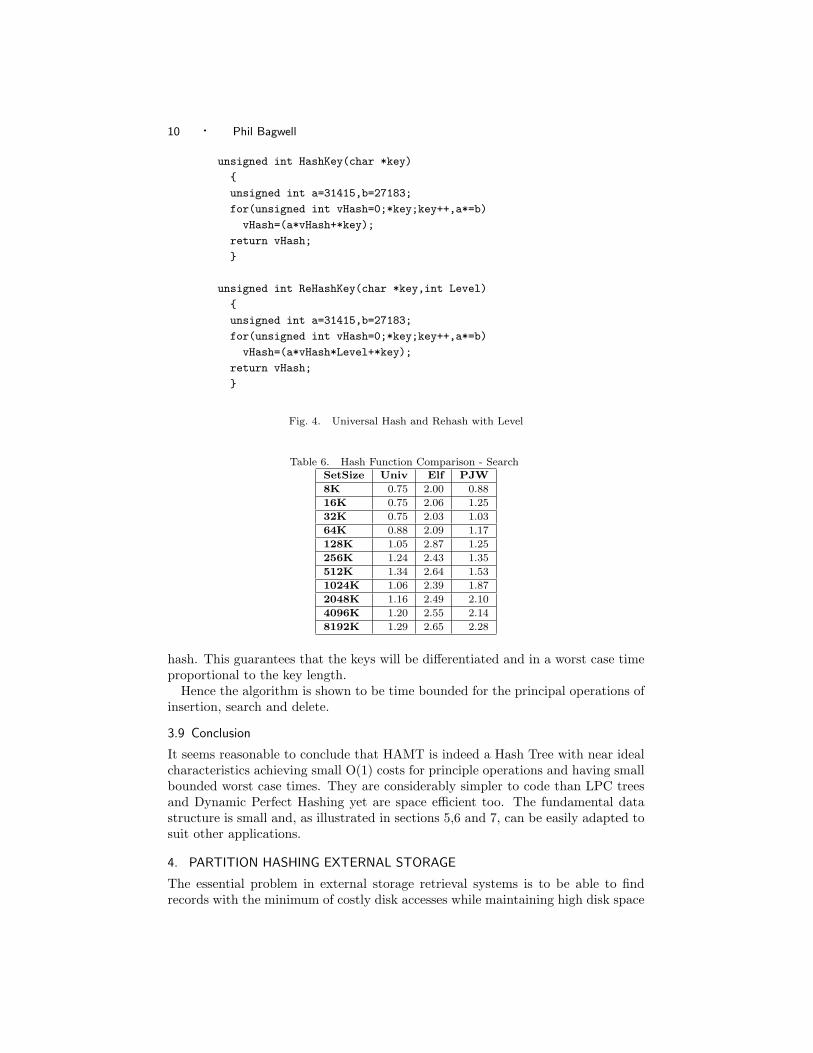
10 · Phil Bagwell

unsigned int HashKey(char *key){unsigned int a=31415,b=27183;for(unsigned int vHash=0;*key;key++,a*=b)

vHash=(a*vHash+*key);return vHash;}

unsigned int ReHashKey(char *key,int Level){unsigned int a=31415,b=27183;for(unsigned int vHash=0;*key;key++,a*=b)

vHash=(a*vHash*Level+*key);return vHash;}

Fig. 4. Universal Hash and Rehash with Level

Table 6. Hash Function Comparison - SearchSetSize Univ Elf PJW8K 0.75 2.00 0.8816K 0.75 2.06 1.2532K 0.75 2.03 1.0364K 0.88 2.09 1.17128K 1.05 2.87 1.25256K 1.24 2.43 1.35512K 1.34 2.64 1.531024K 1.06 2.39 1.872048K 1.16 2.49 2.104096K 1.20 2.55 2.148192K 1.29 2.65 2.28

hash. This guarantees that the keys will be differentiated and in a worst case timeproportional to the key length.

Hence the algorithm is shown to be time bounded for the principal operations ofinsertion, search and delete.

3.9 Conclusion

It seems reasonable to conclude that HAMT is indeed a Hash Tree with near idealcharacteristics achieving small O(1) costs for principle operations and having smallbounded worst case times. They are considerably simpler to code than LPC treesand Dynamic Perfect Hashing yet are space efficient too. The fundamental datastructure is small and, as illustrated in sections 5,6 and 7, can be easily adapted tosuit other applications.

4. PARTITION HASHING EXTERNAL STORAGE

The essential problem in external storage retrieval systems is to be able to findrecords with the minimum of costly disk accesses while maintaining high disk space

Ideal Hash Trees With AMT’s · 11

utilization. The ideal would be 1 access for search (success/failure) or insertionand 100 percent disk space usage for data records. External Hashing, Fagin, Niev-ergelt, Pippenger, and Strong [1979] , B-Trees, R.Bayer and E.M.McCreight [1972]and more recently Linear Hashing, Litwin, Neimat, and Schneider [1993],[Litwinand Schwarz 2000], have striven to do this, Linear Hashing coming close to theideal. Partition Hashing comes closest of all, achieving 1 access for search (suc-cess/failure), 1.1 access for insertion at 80 percent load factor or 2 accesses for loadfactor approaching 90 percent.

In Linear Hashing (LH) a h(C) = C mod N ∗2i hash function is used to distributerecords between buckets and hence control the subsequent splitting required on dataset growth. When a bucket needs to be split i is is set to i + 1 and the recordsdistributed into the new and old bucket accordingly. The problematical issue oflow load factor is offset by using chained overflow buckets to delay splitting at thecost of very few access times to achieve an impressive performance.

In Partition Hashing(PH) a bucket is split into two buckets by moving half ofthe records from the old bucket to the new one. To do this a list of the records iscreated in their key hash order. The mid-point of this list, called the Hash PartitionPoint, has the hash value that divides the number of records equally in two. Therecords in the top half are moved to the new bucket, those in the bottom stay inthe existing one. The Hash Partition value then is kept in a Hash Partition tableassociating this value with the bucket address. If buckets are non-contiguous thenone entry is needed per Bucket. Note that the precision of this partition valueonly needs to be about 5 + lgN bits, where N is the maximum key set size, tosatisfactorily maintain split accuracy.

Partition Hash Table entries may be reduced to the bucket address plus a fewbits by eliminating the redundancy in the leading bits of successive partition hashvalues, Knuth [1998]page 512 and using a single bit indicating free space.

4.1 Search

To find a given record, first compute the keys’ hash. Then find the entry in theHash Partition table where the key hash lies between its Hash Partition value andthe one in the entry above. The desired record is in bucket with the correspondingaddress.

Finding the entry in the Hash Partition table is simpler than it first appears.Because the keys are well distributed, the initial entry e can be found by e = h

hmaxb

and then making a linear search to find the correct record. Here h is the key hash,hmax is the maximum hash value and b the number of bucket entries in the table.Simulation shows the first entry is typically the correct one while in fewer than 10percent of the cases the search continues to an adjacent entry. Note this propertycan be used to remove the requirement for the Hash Partition Table if the bucketsare contiguous and more accesses can be tolerated on search or insert operations.Using a small table of correction offsets improves the hit rate.

4.2 Insert

First a search is performed to find the correct bucket as described in the previoussection. If there is space the new record can be added. However, if the bucket isfull additional space must be found.

12 · Phil Bagwell

Rather than just splitting the bucket on overflow, first a check is made to ascertainif the adjacent Hash Partition table entries have buckets with available space toshare. Then the one with most space is shared with the full bucket by redistributingthe records over the two buckets and updating the Hash Partition value in thetable. The process is identical to the splitting described previously. First a list ofthe records for the two buckets is created in key hash order. The Hash PartitionPoint is defined and then records are moved from the full bucket to the less full onebased on this hash partition value. This simple device delays the need to split andincreases the overall load factor. Only if sharing fails to find space is a split finallyperformed. Simulation shows that about 10 percent of the inserts will need a shareor a split and the load factor stabilizes at just over 80 percent independent of bucketsize. Though using larger buckets extends the number of inserts to stabilization.

At the cost of additional insert assesses load factors approaching 100 percent arepractical. To achieve this the sharing is extended beyond the immediate neighborswhen a full bucket is encountered. The Partition Hash Table is search for up to tplaces above and below the full bucket to find space available in a bucket perhapsa distance s from it. Bucket s is then shared with bucket s − 1, then s − 1 withs − 2, and so on, always moving at least one record, until a space for at least onerecord is finally created in the full bucket. The sharing process will tend to balancethe load factor in the s buckets manipulated in this way.

Table 7 shows the load factors achieved while varying the value of r and thebucket size. The average number of insert accesses that correspond to these loadfactors are shown too. By setting the one parameter t the load factor of the file maybe set to achieve a desired load factor and insert cost relationship. Alternativelya maximum size available for buckets could be set and t increased as the limit isapproached. In this way while the file is small fastest insert times are achieved butas the file limit approached insert times progressively degrade until the file is finallyfull but with a load factor close to 100 percent. These additional insert accessesdoes not change the search cost, remaining constant at one access.

Note that duplicate keys represent a small complication. A single bit flag mustbe added to the Partition Hash Table entry to indicate if the partition Point isa duplicate key. Then, when adding a new record with a duplicate key it can becorrectly positioned at the end of the existing duplicate records. While searching fora record the search can correctly be terminated at the first of the duplicate entries.During shares order is preserved so correct sequencing of records is maintained inthe file.

4.3 Bucket Searches

It has been assumed that the records are stored in a bucket with no particular order.This assumption follows from the fact that a linear search after a bucket has beenloaded from disk still takes a small fraction of the load time. However, buckets canbecome large enough that significant processor time is lost in this linear search orthe buckets are RAM resident. Other methods are then appropriate. For example,records can be placed using linear probe hashing or, for a small space overhead,a list, sorted by hash value, of record pointers can be added to the beginning ofa bucket. Note pointers in this structure need only be lg r bits long where r isthe number of records in the bucket, giving a small overhead of int((lg r) + 1) bits

Ideal Hash Trees With AMT’s · 13

Table 7. Average Insert Accesses and Load Factor %Range(t) r = 2 r = 5 r = 10 r = 20 r = 50 r = 100 r = 5001 1.00/74 1.22/80 1.24/82 1.19/84 1.10/86 1.07/88 1.02/892 1.49/85 1.45/85 1.39/85 1.27/87 1.15/88 1.09/90 1.03/893 1.82/88 1.79/89 1.69/89 1.55/90 1.35/92 1.23/90 1.09/924 2.13/89 2.08/90 1.99/91 1.85/91 1.60/92 1.43/91 1.21/935 2.44/91 2.39/91 2.31/91 2.12/93 1.82/92 1.60/94 1.34/946 2.72/91 2.73/91 2.58/92 2.38/93 2.05/94 1.84/93 1.47/957 3.04/92 2.96/93 2.86/93 2.59/93 2.20/94 1.88/96 1.68/958 3.33/93 3.29/93 3.18/93 2.90/95 2.47/95 2.19/95 1.87/969 3.59/93 3.56/93 3.43/94 3.15/95 2.76/96 2.44/95 2.00/9510 3.91/94 3.89/94 3.59/94 3.42/95 2.97/95 2.50/96 2.32/9720 6.53/96 6.38/96 6.10/95 5.51/97 4.78/95 4.11/97 4.12/9630 8.59/96 8.49/97 8.24/97 7.57/95 6.63/97 5.06/97 5.47/9740 10.77/96 10.14/97 9.85/96 8.99/97 8.57/99 6.54/99 7.00/9750 12.42/97 13.04/97 11.63/98 11.05/98 9.66/96 7.36/98 8.78/97

per record. A given record can then be found using the same method as with theHash Partition Table, namely, the initial entry e is found by e = h−hl

hh−hlr and then

making a linear search to find the correct record. Here r is the number of recordsin a bucket, hl the lower hash partition value and hh the higher partition boundary.Notice too that this is exactly the table needed to support shares and splits.

Where r is large and record length small the overhead of this table may becomeexcessive. An obvious solution is to treat each bucket as a collection of sub-bucketsand create a Hash Partition table for it. The overhead then reduces to one HashPartition Table entry for each sub-bucket and a sub-bucket is found in the sameway as a bucket.

4.4 Client and Server Distributed Files

In Linear Hashing for Distributed Files it is shown how to create large data basesdistributed over any number of servers. Here an outline is given on how to achievethe same functional characteristics using Partition Hashing.

Each server may be considered a ’super bucket’ and the distribution of recordsacross n servers done in the same way as for buckets. A server maintains a ServerPartition Table for all servers. Each entry has the server address, Hash Partitionboundary and the size of its free space.

To use the database the client first requests the Server Partition Table from anyserver, the server addresses and corresponding Hash Partition Values are returned.Then to search for a record the client computes the hash and dispatches the requestto the appropriate server via the Server Partition Table. The server finds the recordusing its own Bucket Partition Table and returns the requested data to the client.

Suppose that a server is running out of storage space. Reference is made to theServer Partition Table to find which Server Hash Partition Table adjacent partnerhas the most available space. A request to share space is made to that partner,the partner agrees and replies with a size to move. The requester now transfersthe buckets, starting from the end of its Bucket Partition Table, to the partner onebucket at a time, until the agreed size is reached. After each bucket transfer hasbeen completed successfully the corresponding Server Partition Entries are sent

14 · Phil Bagwell

to the Partner who adds them to its own Partition Table. Then the requesterremoves the Server Partition Table entry and frees up the bucket and notifies itsother adjacent partner of the Hash Partition change. Any search, insert or deleterequests for the moved bucket are forwarded to the partner who services them oncompletion of the move and returns them. These are then returned to the clientwith the Hash Partition update. A boundary change message is propagated toall the other servers at completion of the share. Notice that this redistributionnegotiation is entirely local to the two servers involved and does not involve theclient or the other servers, although it may cause a knock-on request from thepartner to its adjacent server. In fact any number of servers could be undergoingredistribution simultaneously.

The client meanwhile, unaware of this update makes a further request to find akey using its now out of date Server Partition Table. Doing so it sends the requestto the wrong server, the requested record has been moved to a partner duringthe previous space balancing transaction. The server redirects the request to itsadjacent partner and returns the result of the request to the client together with aServer Partition Table boundary update. The client modifies its Server PartitionTable so that future requests will be directed correctly.

As with bucket load balancing, server load balancing is an asynchronous processand can proceed independently as a background task. Server balancing activitycan be expected to be infrequent and hence Server Partition Table updates rare.A new server coming on line would be added into the Server Partition table whereconvenient and load sharing triggered with adjacent servers. Taking a server off-lineis managed by first moving occupied buckets to adjacent servers and then removingit from the Server Partition Table.

Notice that as with Linear Hashing Server Partition Tables do not need to beperfectly synchronized, differences can be resolved at service request time.

4.5 Conclusion

Partition Hashing builds on the conceptual framework provided by Linear Hash-ing to create algorithms for dynamic external storage more closely approaching theideal. Searches both successful and unsuccessful require just one access while in-serts cost 1.1 accesses for an 80 percent load factor or by varying one parameterload factors approaching 100 percent can be achieved at the cost of extra assesseson insert. When used in a multi-processor environment the distributed updatemechanism appears to be better matched to the ideals outlined by Devine. Devine[1993]

5. SORTED ORDER AMT

In the HAMT the key is hashed before insertion into the tree. However, the entirekey can be treated as a hash. In this case keys will be stored in the trie in sortedorder and become the familiar character trie.

This is a special case of the more general AMT algorithm included in Bagwell[2000]. However, it is still a valuable algorithm as it has a speed and space occu-pancy comparable to the more general algorithm yet uses exactly the same efficientmemory allocation as HAMT. The structure supports all the expected sorted orderfunctions such as ranges, ordered iteration and so on. Table 8 gives times space

Ideal Hash Trees With AMT’s · 15

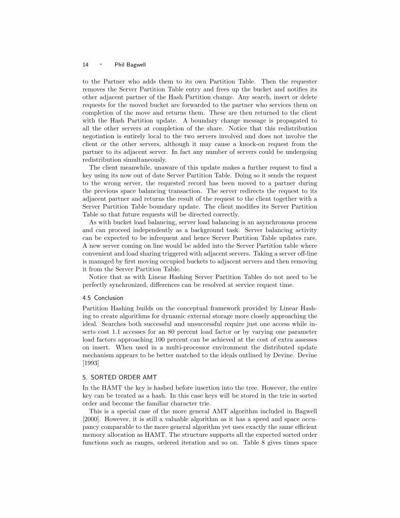
utilization using the same benchmark sets as the HAMT benchmarks in previoustables and can be compared with the TST. The times are expected to be compa-rable and faster than HAMT as with randomly distributed keys they are uniqueafter about logsN characters on average, where s is the cardinality of the alphabet,and this is equivalent to the lgN bits of the hash. However, the key is not hashedfirst, saving the key hashing time and the costly memory accesses to the rest ofthe characters in the key. However, if the keys are not randomly distributed thenthe depth of the trie will grow, requiring more space, take more trie levels andconsequentially more access time.

The root table may be resized automatically too and gains in speed made. How-ever, more care must be taken as typical key sets, symbol tables for example, usea small part of the available alphabet. As an alternative the first n characterscould be hashed and used to index the root hash table. Subsequent characters aretaken without hashing and the sort order is retained. An additional two pointersare required in the root hash table entries, a pointer to the next ordered entry anda pointer to a key containing at least the n character prefix. Then sorted orderfunctions can be undertaken and dynamic shrinking feasible. Since the root tableis infrequently restructured the cost of maintaining the additional order informa-tion is negligible and performance is improved. Further the full key does not needto be examined during resizing. n can be set dynamically allowing the root tableto be resized automatically as with HAMT. This arrangement has not yet beencharacterized.

5.1 Ordered Distributed External Storage

Unsurprisingly the Partition Hashing structure can be adapted for sorted orderrecord storage. If in the above discussion of Partition Hashing and DistributedFiles the lower key is substituted for lower Hash Partition then the same PartitionTables structure and splitting may be used to give a distributed ordered data base.The result provides an interesting alternative to B-Trees but with smoother perfor-mance, higher load factor and no stored dictionary. Performance will be the sameas Partition Hashing but more space could be required in the Partition Table tostore a full key and rapid searches can no longer use direct table indexing. However,replacing the table with a Ordered AMT resolves this problem nicely. Similarly thelist in each bucket is replaced by an AMT too. In both cases no keys then needto be stored in the trie hence making it only a little more costly than PartitionHashing.

Further research is needed to complete the characterization. However, the struc-ture looks promising.

6. IP ROUTING

IP routers must select an appropriate outgoing route based on the IP address of anincoming packet. The IP address is 32 bits long and for public routing, for classA, B and C sub-nets only the first 24 bits need be considered in order to route amessage to the appropriate sub-net. The problem therefore becomes to associatetarget route for each of the incoming packets from the first 24 bits of the address.Nilsson and Karlsson [1998] describe a high performance algorithm to do just thiswhile here I demonstrate that a comparable performance algorithm can be created

16 · Phil Bagwell

Table 8. Ordered Insert, Search and SizeAMT AMT AMT AMT TST TST

SetSize Insert Search Total Pool Free Pool Insert Search8K 3.40 0.59 14K 2K 10.23 2.7816K 3.74 0.69 27K 4K 11.08 2.9932K 3.67 0.78 50K 8K 12.67 3.2764K 3.62 0.86 88K 13K 14.72 3.57128K 3.95 1.02 171K 25K 14.59 3.87256K 4.76 1.05 382K 58K 13.76 4.16512K 5.16 1.20 860K 117K 13.07 4.511024K 4.59 1.27 1670K 238K 12.26 4.862048K 4.68 1.31 2927K 425K – –4096K 5.19 1.30 5646K 839K – –8192K 6.33 1.34 12006K 1755K – –

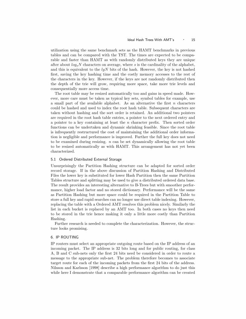
simply with the AMT data structure.Fig 6 illustrates the data structure to be used and is clearly a special case of the

hash tree previously described. The root table is created with a length of 224

32 thatis to have 219 entries requiring 4 Mb. Each entry is either empty, contains a routeor is a 32 entry sub-trie and pointer. To identify a route for an IP address thefirst 19 bits are used as an index into the root table and then the remaining 5 bitsused to select the entry in the sub-trie. Unknown addresses can be identified anddropped with just the index and a bit test on the bit map.

The IP routing table can be updated using the same basic insertion algorithmsdescribed in the hash tree above while the non-critical memory allocation is left tothe system.

For the new address format with IPV6 using 128 bit addresses a HAMT wouldprovide an efficient solution with O(1) access.

// IP is the IP addressif((E=RootTbl[IP>>13])&&(E->Map&(1<<((IP>>8)&0x1F)))Route=E->Base+CTPOP(E->Map&(~((~0)<<((IP>>8)&0x1F));

else // Failed

Fig. 5. Code fragment for IP dispatch

7. CLASS-SELECTOR DISPATCH

In modern object oriented language design it is desirable to be able to create Class-Selector tables dynamically. As classes inherit from super classes the compiler mustmaintain a table valid method selectors. At run time it must be a fast operationto map a class-selector pair to an actual method and verify that it is also validor perhaps dynamically load new classes with their associated methods. A goodsolution to the compilers static task is described in Driesen [1993] and Driesen andHolzle [1995]. A comparable solution to the problem is simply constructed with anAMT data structure yet has the added property of being dynamically updateable.

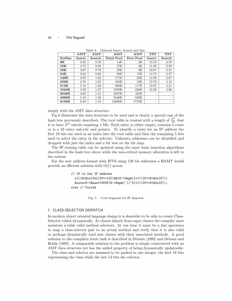
The class and selector are assumed to be packed in one integer, the first 18 bitsrepresenting the class while the last 14 bits the selector.

Ideal Hash Trees With AMT’s · 17

Root Route Table

-

Map BaseRoute RouteMap BaseRoute RouteMap Base

Sub-Table

RouteRouteRouteRoute

Fig. 6. IP Routing Table

Root Class-Selector Table

-

Empty EmptyMap BaseMap BaseMap BaseMap Base

Sub-Table

MethodMethodMethodMethod

Fig. 7. Class-Selector Table

It is initially assumed that there will be 2c classes with any of 2s selectors. Anempty root table is then created of length 2(c+s−5). As classes and methods arecompiled they are added to the table. The last c bits of the class is combined withthe last s bits of the selector and the method pointer entry made in the appropriatenode of the sub-trie. For method pointer look up the same process is followed. cclass bits are combined with s selector bits. The first c+s−5 bits are used to indexinto the root table while the last 5 bits index into the sub-trie. Either the methodpointer is retrieved or the class/selector is invalid.

// Class C, Selector SIndex= (C<<(s-5))|(S>>5);if((E=RootTbl[Index])&&(E->Map&(1<<(S&0x1F)))MethodPtr=E->Base+CTPOP(E->Map&(~((~0)<<(S&0x1F));

else // Failed

Fig. 8. Code fragment for Method dispatch

The class-selector table can be updated using the same basic insertion algorithmsdescribed in the hash tree above while the non-critical memory allocation is left tothe system.

However, the number of classes or selectors may overflow the allocate 2c or 2s

entries initially reserved. When this occurs the table can be easily restructuredto accommodate the additional entries. Suppose for the moment that the classes

18 · Phil Bagwell

exceed 2c. The new class limit is set to c′ where c′ = c + 1 and thereby double thenumber of allowed classes. A new root table is created with a length of 2(c′+s−5),the old root table entries are copied to the new one and the old table deleted. Futuresearches will use c’ bits to identify the class. Similarly if the selectors overflow 2s

the new selector limit is set to s′ where s′ = s+1. A new root table is created withlength c + s′ − 5 and the entries copied from the old table to the new one, taking sentries at a time from the old table and inserting these in the new one. After eachmove s entries are left empty, for future selector insertions, before copying the nextblock.

Although apparently longer this algorithm makes the same number of memoryaccesses as the row displacement algorithm referred to above, yet is dynamic, allowsrun time updating and using memory progressively. With an additional memoryaccess, more memory may be conserved by allowing the trie one more level.

8. PERFORMANCE COMPARISONS

All the algorithms were tested with the same wide variety of unique key sets. Thesets were in random, sorted order or semi-ordered sequence. The test sets wereproduced using a custom pseudo random number generator. These were createdby first generating a random prime number which was repetitively added to aninteger to produce a sequence of 32 bit integer keys. For high value prime numbersthis sequence is pseudo random while for low value prime numbers the sequence isordered. Values in between generate semi-ordered sequences.

An alphabet cardinality of 250 was used as a radix to convert the integer key to astring of characters. Additional characters were added to create an eight-characterkey. All the test results were for 8 character key sets created in this manner.

The technique ensures unique key production and allows search test key sets tobe generated with different sequences to those used during insertion yet from thesame key set.

Each algorithm’s performance was measured on an Intel P2, 400 MHz with 512Mbof memory, NT4 and VC6. Times shown are in µS per insert or search for 8character keys averaged across 50 test key sets. CTPOP was emulated using thealgorithm in Fig 2.

The external disk and distributed storage algorithms were tested by simulation.No actual timings were made but the critical characteristic of disk accesses persearch and insert together with load factor was monitored in the simulation modelover a large number of runs.

ACKNOWLEDGMENTS

I would like to thank Prof. Martin Odersky and Christoph Zenger at the Labo.Des Methodes de Programmation (LAMP), EPFL, Switzerland for their review ofthe draft paper and valuable comments.

REFERENCES

Bagwell, P. 2000. Fast and space efficient trie searches. Technical Report, EPFL Swtzer-land .

Bentley, J. and Sedgewick, R. 1997. Fast algorithms for sorting and searching strings.In Eighth Annual ACM-SIAM Symposium on Discrete Algorithms (1997), SIAM Press

Ideal Hash Trees With AMT’s · 19

(1997).Devine, R. 1993. Design and implementation of DDH: A distributed dynamic hashing

algorithm. Lecture Notes in Computer Science 730, 101–114.Dietzfelbinger, M., Karlin, A., Mehlhorn, K., auf der Heide, F. M., Rohnert, H.,

and Tarjan, R. E. 1994. Dynamic perfect hashing: Upper and lower bounds. SIAMJournal on Computing 23, 4, 738–761.

Driesen, K. 1993. Selector table indexing sparse arrays. In Conference on Object-Oriented(1993), pp. 259–270.

Driesen, K. and Holzle, U. 1995. Minimizing row displacement tables. In OOPSLA 95(1995).

Fagin, R., Nievergelt, J., Pippenger, N., and Strong, H. R. 1979. Extendible hashing— A fast access method for dynamic files. ACM Transactions on Database Systems 4, 3,315–344.

Fredkin, E. 1960. Trie memory. Communications of the ACM 3, 490–499.Knuth, D. 1998. The Art of Computer Programming, volume 3: Sorting and Searching,

2nd Ed. Addison-Wesley, Reading, MA.Larson, P. 1988. Dynamic hash tables. In Comm. of ACM (CACM), Volume 31 (1988),

pp. 446–457.Litwin, W., Neimat, M., and Schneider, D. 1993. Linear hashing for distributed files.

ACM-SIGMOD Intl. Conf. on Management of Data, 1993.Litwin, W. and Schwarz, T. 2000. LH* RS : A high-availability scalable distributed data

structure using reed solomon codes. In SIGMOD Conference (2000), pp. 237–248.Nilsson, S. and Karlsson, G. 1998. Fast address look up for internet routers. In Proceed-

ings of IEEE Broadband Communications 98 (April 1998).Nilsson, S. and Tikkanen, M. 1998. Implementing a dynamic compressed trie. In 2nd

Workshop on Algorithm Engineering WAE 98 Saarbruecken Germany (August 1998).R.Bayer and E.M.McCreight. 1972. Organization and maintenance of large ordered in-

dices. Acta Informatica 1, 3, 173–189.Sedgewick, R. 1998. Algorithms in C++, 3rd Ed. Addison-Wesley, Reading, MA.