Embed Size (px)
Citation preview
Automation and Remote Control, Vol. 63, No. 3, 2002, pp. 433–448. Translated from Avtomatika i Telemekhanika, No. 3, 2002, pp. 97–113.Original Russian Text Copyright c© 2002 by Karasev, Solozhentsev.
DISCRETE SYSTEMS
Identification of the Logical-and-Probabilistic
Risk Models of Structurally Complex Systems with
Groups of Inconsistent Events
V. V. Karasev and E. D. Solozhentsev
Institute of Mechanical Engineering Problems, Russian Academy of Sciences, St. Petersburg, RussiaReceived October 30, 2000
Abstract—The theory of identification of the logical-and-probabilistic risk models of struc-turally complex systems with groups of inconsistent events was presented. For the logical-and-probabilistic risk models, their high precision and stability based on the groups of inconsistentevents (Bayes formulas) and a well-organized risk polynomial was substantiated. Precision andstability of the logical-and-probabilistic risk models was compared with the well-known methodsof classification of objects. For systems of various logical complexity, examples of identificationand analysis of the logical-and-probabilistic models were presented.
1. INTRODUCTION
The theory of identification of the logical-and-probabilistic (LP) risk models is regarded as anextension of the reliability theory as applied to the system elements and output characteristics thathave more than one level of values. This path of research which is known as “Reliability Analysis andOptimization of Multi-state Systems” [1] is developed mostly for forecasting the possible extensionof life of the technical systems.
Consideration is given to the structurally complex systems such as banks, business, or diagnosticsystems where risk is an everyday event and where a sufficient statistics about the risk objects hasbeen accumulated. By risk is meant the probability of failure. Consideration is given to the staticrisk problem. Dynamics of the processes is taken into account by retraining the risk model withthe arrival of new information about the risk objects. The discrete nonparametric probabilitydistributions for the events from the groups of inconsistent events (GIE) are used.
The propositions presented below extend the well-known I.A. Ryabinin’s engineering LP-theoryof reliability and safety [2–4]. However, new notions are introduced and new risk problems forbusiness and engineering are formulated:
(1) consideration is given to the initializing events at many levels; their number is finite andamounts to ten; the resulting event can also have more than one level;
(2) the logical risk models (L-models) are considered as associative models based on the commonsense of relations between events;
(3) the problems of parametric and structural identification of the risk LP-models—determina-tion of the probabilities of initiating events and modification of the L-model (L-function) itself—aresolved using the statistical data;
(4) new analytic problems are tackled by analyzing the contributions of initiating events in themean risk of the objects, precision of the risk LP-model, and so on; and
(5) the problems of risk control are formulated.Risk will be considered as a complex problem [5] consisting of (1) evaluation of the failure
risk; (2) classification of the object or its state on the “good–bad” scale by the value of risk;
0005-1179/02/6303-0433$27.00 c© 2002 MAIK “Nauka/Interperiodica”
434 KARASEV, SOLOZHENTSEV
(3) determination of the risk cost; (4) analysis of the contributions of events into the risk of theobject; (5) analysis of the contributions of events into the mean risk of the objects; and (6) analysisof the contributions of events into the precision of the risk LP-model.
Consideration is given to the uniform risk objects (for example, credit risks) or states of thesame system at different time instants (the system is up and operable; the system is down butoperable; the system is down but restorable; the system is up but its operation is inadvisable). Therisk object is described by a large set of attributes (up to 100). The least number of attributesis chosen so as to provide their weak correlation and enable one to regard them as independent.Each attribute has more than one gradation (numbers of values), their number varying from 2to 20. Gradations are linearly unordered; for example, it is impossible to assert that gradation 3 isinferior or superior to gradation 4. The final event also has more than one—in the simplest case,two, failure or success—gradations. Information about the risk objects can be conveniently definedas a tabular “object–attributes” database whose rows contain the objects, columns, the attributes,and the entries, the attribute gradations [5]. For example, if the jth attribute has four gradations 1,2, 3, and 4, then the entry for the ith row (object) and the jth column (attribute) contains one ofthem. After identification of the risk LP-model by the statistical data, it is used to evaluate therisks of new objects and to solve the problems of analysis and risk control.
2. BASIC DEFINITIONS
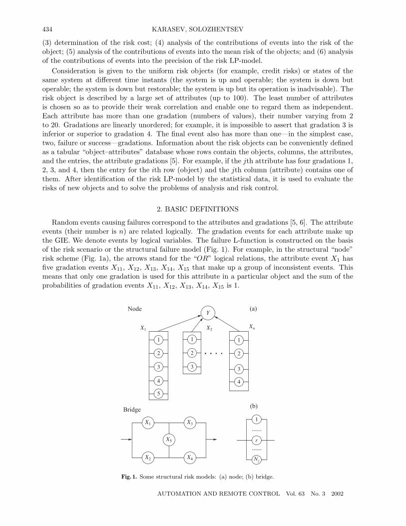
Random events causing failures correspond to the attributes and gradations [5, 6]. The attributeevents (their number is n) are related logically. The gradation events for each attribute make upthe GIE. We denote events by logical variables. The failure L-function is constructed on the basisof the risk scenario or the structural failure model (Fig. 1). For example, in the structural “node”risk scheme (Fig. 1a), the arrows stand for the “OR” logical relations, the attribute event X1 hasfive gradation events X11, X12, X13, X14, X15 that make up a group of inconsistent events. Thismeans that only one gradation is used for this attribute in a particular object and the sum of theprobabilities of gradation events X11, X12, X13, X14, X15 is 1.
Fig. 1. Some structural risk models: (a) node; (b) bridge.
AUTOMATION AND REMOTE CONTROL Vol. 63 No. 3 2002
IDENTIFICATION OF THE LOGICAL-AND-PROBABILISTIC RISK MODELS 435
The structural risk model can be equivalent to a physical (electrical, for instance) system,associative if based on the common sense, or mixed. The common sense in the “node” failure riskmodel (Fig. 1a) lies in that a failure appears upon occurrence of one, any two, . . . , or all initiatingevents. The L-functions of various complexity related by ANDs, ORs, and NOT s and having cyclesand repeated elements correspond to the structural risk schemes. After orthogonalization, any riskL-function is representable as the probabilistic polynomial or probabilistic model (P-model) or theprobabilistic function enabling one to calculate the risk if the probabilities of the initiating eventsare known.
The binary logical variable Xj is 1 with the probability Pj if the jth attribute resulted in failureand 0 with the probability Qj = 1− Pj, otherwise. The binary logical variable Xjr correspondingto the r-gradation of the jth attribute is 1 with the probability Pjk and 0 with the probabilityQjr = 1 − Pjr, otherwise. The vector X(i) = (X1,X2, . . . ,Xj , . . . ,Xn) describes an arbitraryith object from the “object–attributes” table. When defining a particular ith object, one mustreplace the logical variables X1, X2, . . . ,Xj , . . . ,Xn by the corresponding logical variables Xjr forthe gradations of the attributes of the specific object under study. Therefore, the particular objectX(i) is defined by the gradations of its attributes. One can readily see that the maximal numberof different objects is Nmax = N1 × N2 × · · · × Nj × · · · × Nn, where N1, N2, . . . , Nj , . . . are thenumbers of gradations in the attributes. The table mostly contains different objects, that is, objectsdescribed by different sets of gradations.
We set down in the general form the L-function of object failure
Y = Y (X1,X2, . . . ,Xj , . . . ,Xn) (1)
and the P-function
Pi{Y = 1 |X(i)} = Ψ(P1, P2, . . . , Pj , . . . , Pn), i = 1, N, (2)
of failure of the object defined by the vector X(i).For each gradation event, we consider three probabilities in the GIE: the relative frequency Wjr
of gradation in the objects of the “object–attributes” table; the probability P1jr of the gradationevent in the GIE; and the probability Pjr of the gradation event substituted into (2) for Pj. Wedetermine these probabilities for the j-GIE:
Wjr = P{Xjr = 1};Nj∑r=1
Wjr = 1; r = 1, Nj ; (3)
P1jr = P{Xjr = 1 |Xj = 1};Nj∑r=1
P1jr = 1; r = 1, Nj ; (4)
Pjr = {Xj = 1 |Xjr = 1}; r = 1, Nj . (5)
The mean values of the of the probabilities Wjr, P1jr, and Pjr for the gradations in the GIE areas follows:
Wjm = 1/Nj ; Pjm =Nj∑r=1
PjrWjr; P1jm =Nj∑r=1
P1jrWjr; (6)
the mean a priori risk Paν and the mean calculated risk Pm of the objects are as follows:
Paν = Nb/N ; Pm =
(N∑i=1
Pi
)/N, (7)
where N and Nb are, respectively, the total number of objects in the table and the number of “bad”ones.
AUTOMATION AND REMOTE CONTROL Vol. 63 No. 3 2002
436 KARASEV, SOLOZHENTSEV
Relationship between the probabilities Pjr and P1jr. The risk of object Pi obey formula (2)where the probabilities Pjr are substituted for Pj . The probabilities Pjr will be evaluated foralgorithmic iterative learning (identification) of the risk P-model from the data of the “object–attributes” table. The risk P-model can be trained with or without regard for the GIE.
If training disregards the GIE, then the probabilities Pjr and P1jr are trivially related as
P1jr = Pjr/
Nj∑r=1
Pjr; r = 1, Nj , (8)
that is, in the optimization problem of the algorithmic iterative training of the risk P-model by thedata of the “object–attributes” table it is assumed that the probabilities Pjr are evaluated directlyand the probabilities P1jr are calculated from (8) for reference. Here, the number of independentevaluated probabilities Pjr is as follows:
Nind =n∑j=1
Nj. (9)
If the GIE is taken into account for training, then one has first to determine the probabilities P1jrmeeting condition (4) and then go from them to the probabilities Pjr, the number of independentevaluated probabilities Pjr being as follows:
Nind =n∑j=1
Nj − n. (10)
Let us consider the possible relationships between the probabilities Pjr and P1jr for one GIEupon training the risk P-model. At each step of iterative training of the risk P-model from thestatistical data, the relation between the probabilities Pjr and P1jr of gradation events can beconstructed on the basis of expressions (3–5) using the well-known rule for conditional probabilities(Bayes formula):
P1jr = (Pjr ×Wjr)/Pjm; r = 1, Nj . (11)
If the “object–attributes” table contained all possible different objects (their maximum numberwas noted above to be Nmax), then for each attribute in the GIE the frequencies of gradationswould be the same and equal to the mean value of frequencies in the GIE (6). In effect, the numberof objects in the “object–attributes” table always is much smaller, and therefore, gradations withzero or negligible frequencies Wjr occur. Hence, the Bayes formula is unsuitable for relating theprobabilities Pjr and P1jr, and other formulas will be established to this end.
In distinction to (11), in the first formula the frequency Wjr is replaced by the mean gradationfrequency Wjm in the GIE to which Wjr tends with the number of objects in the table:
P1jr = (Pjr ×Wjm)/Pjm; r = 1, Nj . (12)
In distinction to (11), in the second formula the mean frequency Wjm in the GIE was introducednot only instead of Wjr, but to calculate Pjm. Then, we get the well-known formula (8).
The third formula was obtained under the assumption that the relationship between the prob-abilities P1jr and Pjr is constant for the GIE. Then, the relationship between the probabilitiesPjr and P1jr for gradations is expressed in terms of the mean values of the probabilities Pjm andP1jm:
P1jr = (Pjr × P1jm)/Pjm = Kj × Pjr; r = 1, Nj , (13)
where Kj = P1jm/Pjm. Formulas (11) and (12) are unsuitable for a limited amount of statisticaldata. In what follows, we make use only of (13) relating the probabilities P1jr and Pjr.
AUTOMATION AND REMOTE CONTROL Vol. 63 No. 3 2002
IDENTIFICATION OF THE LOGICAL-AND-PROBABILISTIC RISK MODELS 437
3. GIE AND THE BAYES FORMULA
According to what was said above, a special discussion is required to establish a relationshipbetween the GIE and the Bayes formula. In the Bayes formula, the following notation is usuallyused. After the event A, the hypothesis Hk has the probability
P (Hk/A) = (P (Hk)× P (A/Hk))/P (A), (14)
where P (A) =m∑i=1
P (Hi) × P (A/Hi), the hypotheses Hi(i = 1, 2, . . . , k, . . . ,m) making up a
complete GIE.The risk problems usually deal with many GIEs (1, 2, . . . , j, . . . , n), each group making for Xj
the complete GIE of Xjr (r = 1, 2, . . . , Nj). Therefore, the following notation equivalent to (14)and (3–6) was introduced for the jth GIEs for simplicity:
Event A ≡ Attribute event Xj ; Probability P (Hk/A) ≡ P1jr;Hypothesis Hk ≡ Gradation event Xjr; Probability P (A/Hk) ≡ Pjr;Probability P (Hk) ≡Wjr; Probability P (A) ≡ Pjm.
With this notation, the Bayes formula (14) is representable for the jth GIE as (11). To tackle theproblem of optimization (identification) of the risk LP-model by the statistical data, formula (11)is represented differently: in the left side of the equality we set down the a posteriori and not thea priori probability of the hypothesis (gradation event):
Pjr = (P1jr × Pjm)/Wjr. (15)
We already took note of the fact that if the probabilities Wjr for some gradation events in theGIE are zero or negligible (because of insufficiency of the statistical data), then one encountersdifficulties in using the Bayes formula because the denominator in (15) can turn out to be zero.
Example 1. Let us consider a complete set of uniform “node” risk objects with three attributeevents X1, X2, X3 having two gradations 1 and 2 each. The number of different objects in thecomplete set is N = 23 = 8. The logical and probabilistic risk functions for each of the objects areas follows:
Y = X1 ∨X2 ∨X3; P{Y = 1} = P1 + P2(1− P1) + P3(1− P1)(1− P2).
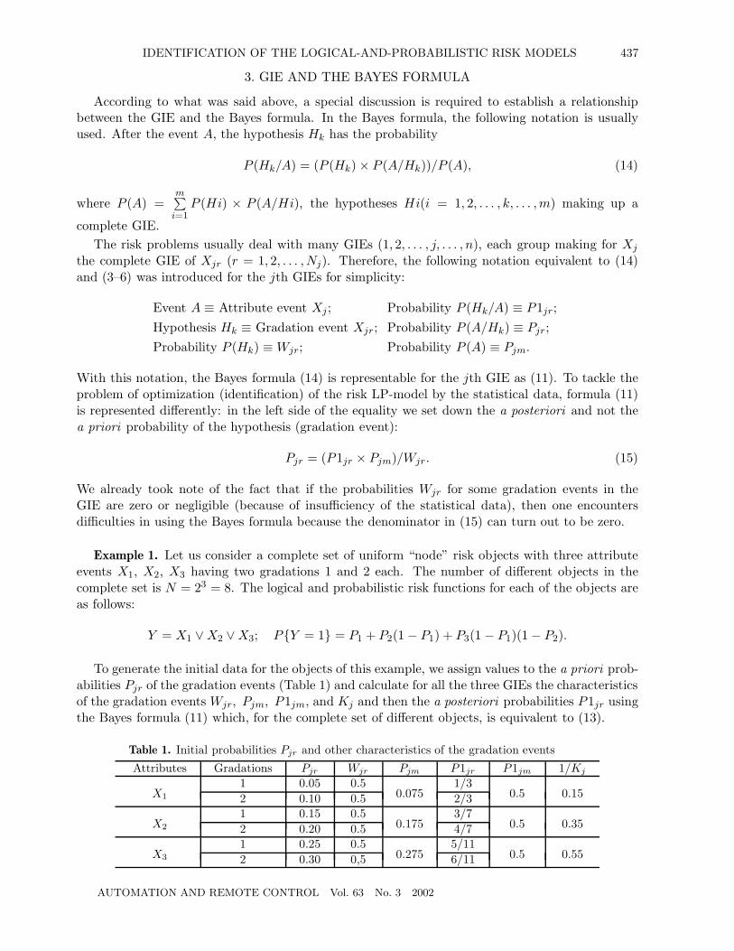
To generate the initial data for the objects of this example, we assign values to the a priori prob-abilities Pjr of the gradation events (Table 1) and calculate for all the three GIEs the characteristicsof the gradation events Wjr, Pjm, P1jm, and Kj and then the a posteriori probabilities P1jr usingthe Bayes formula (11) which, for the complete set of different objects, is equivalent to (13).
Table 1. Initial probabilities Pjr and other characteristics of the gradation events
Attributes Gradations Pjr Wjr Pjm P1jr P1jm 1/Kj
X1
1 0.05 0.50.075
1/30.5 0.152 0.10 0.5 2/3
X2
1 0.15 0.50.175
3/70.5 0.352 0.20 0.5 4/7
X3
1 0.25 0.50.275
5/110.5 0.552 0.30 0,5 6/11
AUTOMATION AND REMOTE CONTROL Vol. 63 No. 3 2002
438 KARASEV, SOLOZHENTSEV
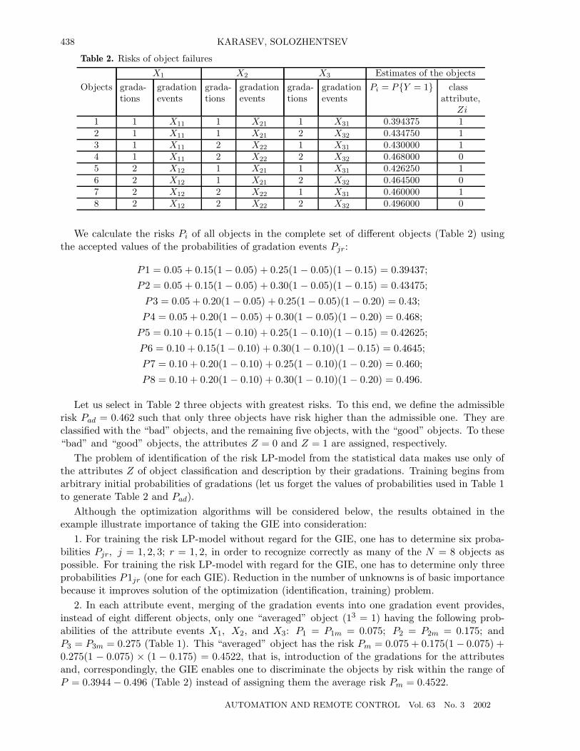
Table 2. Risks of object failures
X1 X2 X3 Estimates of the objectsObjects grada-
tionsgradationevents
grada-tions
gradationevents
grada-tions
gradationevents
Pi = P{Y = 1} classattribute,
Zi1 1 X11 1 X21 1 X31 0.394375 12 1 X11 1 X21 2 X32 0.434750 13 1 X11 2 X22 1 X31 0.430000 14 1 X11 2 X22 2 X32 0.468000 05 2 X12 1 X21 1 X31 0.426250 16 2 X12 1 X21 2 X32 0.464500 07 2 X12 2 X22 1 X31 0.460000 18 2 X12 2 X22 2 X32 0.496000 0
We calculate the risks Pi of all objects in the complete set of different objects (Table 2) usingthe accepted values of the probabilities of gradation events Pjr:
P1 = 0.05 + 0.15(1 − 0.05) + 0.25(1 − 0.05)(1 − 0.15) = 0.39437;P2 = 0.05 + 0.15(1 − 0.05) + 0.30(1 − 0.05)(1 − 0.15) = 0.43475;P3 = 0.05 + 0.20(1 − 0.05) + 0.25(1 − 0.05)(1 − 0.20) = 0.43;P4 = 0.05 + 0.20(1 − 0.05) + 0.30(1 − 0.05)(1 − 0.20) = 0.468;P5 = 0.10 + 0.15(1 − 0.10) + 0.25(1 − 0.10)(1 − 0.15) = 0.42625;P6 = 0.10 + 0.15(1 − 0.10) + 0.30(1 − 0.10)(1 − 0.15) = 0.4645;P7 = 0.10 + 0.20(1 − 0.10) + 0.25(1 − 0.10)(1 − 0.20) = 0.460;P8 = 0.10 + 0.20(1 − 0.10) + 0.30(1 − 0.10)(1 − 0.20) = 0.496.
Let us select in Table 2 three objects with greatest risks. To this end, we define the admissiblerisk Pad = 0.462 such that only three objects have risk higher than the admissible one. They areclassified with the “bad” objects, and the remaining five objects, with the “good” objects. To these“bad” and “good” objects, the attributes Z = 0 and Z = 1 are assigned, respectively.
The problem of identification of the risk LP-model from the statistical data makes use only ofthe attributes Z of object classification and description by their gradations. Training begins fromarbitrary initial probabilities of gradations (let us forget the values of probabilities used in Table 1to generate Table 2 and Pad).
Although the optimization algorithms will be considered below, the results obtained in theexample illustrate importance of taking the GIE into consideration:
1. For training the risk LP-model without regard for the GIE, one has to determine six proba-bilities Pjr, j = 1, 2, 3; r = 1, 2, in order to recognize correctly as many of the N = 8 objects aspossible. For training the risk LP-model with regard for the GIE, one has to determine only threeprobabilities P1jr (one for each GIE). Reduction in the number of unknowns is of basic importancebecause it improves solution of the optimization (identification, training) problem.
2. In each attribute event, merging of the gradation events into one gradation event provides,instead of eight different objects, only one “averaged” object (13 = 1) having the following prob-abilities of the attribute events X1, X2, and X3: P1 = P1m = 0.075; P2 = P2m = 0.175; andP3 = P3m = 0.275 (Table 1). This “averaged” object has the risk Pm = 0.075 + 0.175(1 − 0.075) +0.275(1 − 0.075) × (1 − 0.175) = 0.4522, that is, introduction of the gradations for the attributesand, correspondingly, the GIE enables one to discriminate the objects by risk within the range ofP = 0.3944 − 0.496 (Table 2) instead of assigning them the average risk Pm = 0.4522.
AUTOMATION AND REMOTE CONTROL Vol. 63 No. 3 2002
IDENTIFICATION OF THE LOGICAL-AND-PROBABILISTIC RISK MODELS 439
3. The modified Bayes formula (13) relating the probabilities in the GIE under limited amountof statistical information must be used for training the risk LP-model. It is namely this noveltythat makes training of the risk LP-model successful and optimal in a sense.
4. RISK MEASURES AND RISK COST
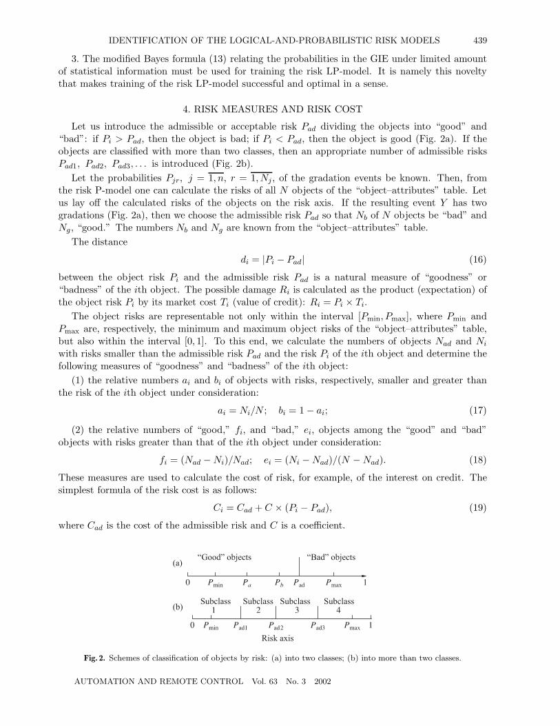
Let us introduce the admissible or acceptable risk Pad dividing the objects into “good” and“bad”: if Pi > Pad, then the object is bad; if Pi < Pad, then the object is good (Fig. 2a). If theobjects are classified with more than two classes, then an appropriate number of admissible risksPad1, Pad2, Pad3, . . . is introduced (Fig. 2b).
Let the probabilities Pjr, j = 1, n, r = 1, Nj , of the gradation events be known. Then, fromthe risk P-model one can calculate the risks of all N objects of the “object–attributes” table. Letus lay off the calculated risks of the objects on the risk axis. If the resulting event Y has twogradations (Fig. 2a), then we choose the admissible risk Pad so that Nb of N objects be “bad” andNg, “good.” The numbers Nb and Ng are known from the “object–attributes” table.
The distance
di = |Pi − Pad| (16)
between the object risk Pi and the admissible risk Pad is a natural measure of “goodness” or“badness” of the ith object. The possible damage Ri is calculated as the product (expectation) ofthe object risk Pi by its market cost Ti (value of credit): Ri = Pi × Ti.
The object risks are representable not only within the interval [Pmin, Pmax], where Pmin andPmax are, respectively, the minimum and maximum object risks of the “object–attributes” table,but also within the interval [0, 1]. To this end, we calculate the numbers of objects Nad and Ni
with risks smaller than the admissible risk Pad and the risk Pi of the ith object and determine thefollowing measures of “goodness” and “badness” of the ith object:
(1) the relative numbers ai and bi of objects with risks, respectively, smaller and greater thanthe risk of the ith object under consideration:
ai = Ni/N ; bi = 1− ai; (17)
(2) the relative numbers of “good,” fi, and “bad,” ei, objects among the “good” and “bad”objects with risks greater than that of the ith object under consideration:
fi = (Nad −Ni)/Nad; ei = (Ni −Nad)/(N −Nad). (18)
These measures are used to calculate the cost of risk, for example, of the interest on credit. Thesimplest formula of the risk cost is as follows:
Ci = Cad + C × (Pi − Pad), (19)
where Cad is the cost of the admissible risk and C is a coefficient.
Fig. 2. Schemes of classification of objects by risk: (a) into two classes; (b) into more than two classes.
AUTOMATION AND REMOTE CONTROL Vol. 63 No. 3 2002
440 KARASEV, SOLOZHENTSEV
5. IDENTIFICATION OF THE RISK LP-MODEL
Identification of the risk P-model lies in determining the optimal probabilities Pjr, j = 1, n;r = 1, Nj , corresponding to the gradation events. The problem of identification (training) of therisk P-model is stated as follows.
Formulation of the problem. Given are the “object–attributes” table with Ng “good” and Nb
“bad” objects and the risk P-model (2). Needed is to determine the probabilities Pjr, j = 1, n;r = 1, Nj , for the gradation events and the admissible risk Pad dividing the objects into “good”and “bad.”
The target function (TF): the number of correctly classified objects must be as high as possible:
F = Nbs +Ngs = MAX, (20)
where Nbs and Ngs are the respective numbers of objects classified as “good” and “bad” both bythe statistics and the P-model (coinciding estimates). We note that it is apparent from (20) thatthe errors or precision indices of the risk P-model in classifying the “good,” Eg, and “bad,” Eb,objects and the model in the whole, Em, are as follows:
Eg = (Ng −Ngs)/Ng; Eb = (Nb −Nbs)/Nb; Em = (N − F )/N. (21)
Constraints:(1) the probabilities Pjr must satisfy the condition
0 < Pjr < 1, j = 1, n; r = 1, Nj ; (22)
(2) the mean risks of the objects by the model, Pm, and table, Paν , must be equal; in the courseof training step, we correct the probabilities Pjr by the formula
Pjr = Pjr × (Paν/Pm); j = 1, n; r = 1, Nj ; (23)
(3) the admissible risk Pad must be determined for the given ratio of incorrectly classified “good”and “bad” objects (this requirement stems from the nonequivalence of the losses of assets underincorrect classification of “good” and “bad” objects):
Egb = (Ng −Ngs)/(Nb −Nbs); and (24)
(4) according to the well-known results of the recognition theory, the minimum admissiblenumber of different objects (with different gradations) in the table must meet the conditionNmin > 20× n.
Algorithm of solution. The formulated problem of identification of the risk P-models has somedistinctions and difficulties: (1) the TF depends on many positive real parameters Pjr (for instance,there were 94 parameters in one of the risk problems); (2) the TF assumes integer values and isstepwise; (3) its derivatives with respect to Pjr is noncomputable; (4) owing to the structure of therisk P-models, the TF has local extrema; and (5) upon seeking the optimum Fmax, it is impossibleto give positive/negative increments to all parameters Pjr because this affects the mean risk.
The problem of identification will be solved algorithmically. An iterative algorithm generatesP1jr to maximize F . We choose appropriate values for the calculated number of “good,” Ngc, and“bad,” Nbc = N − Ngc, objects. For the procedure below, these values are constant. We denotethe numbers of optimizations by 0, 1, . . . , ν, . . . ,Nopt.
Initial values. Let us define the initial values P 0jr and P10
jr, j = 1, n; r = 1, Nj , calculateP 0jm and P10
jm from (6), assign to the TF a small value, for example, F = PaνN , and calculateKj = P 0
jm/P10jm.
AUTOMATION AND REMOTE CONTROL Vol. 63 No. 3 2002
IDENTIFICATION OF THE LOGICAL-AND-PROBABILISTIC RISK MODELS 441
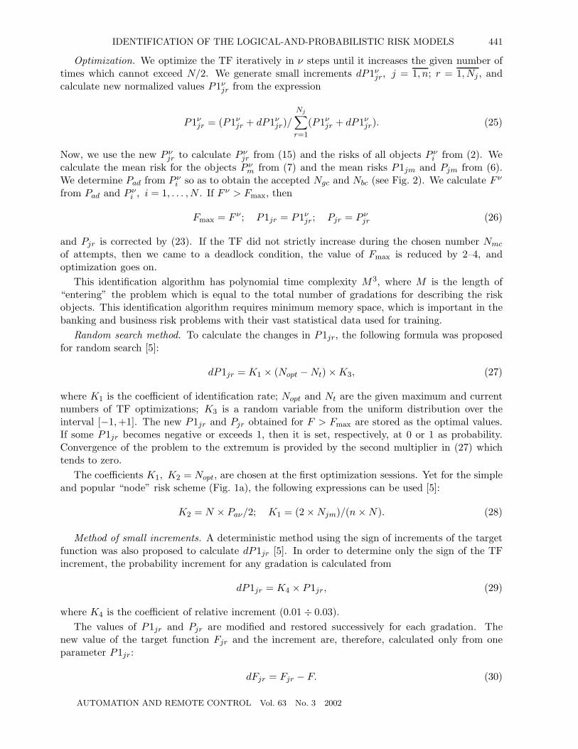
Optimization. We optimize the TF iteratively in ν steps until it increases the given number oftimes which cannot exceed N/2. We generate small increments dP1νjr, j = 1, n; r = 1, Nj , andcalculate new normalized values P1νjr from the expression
P1νjr = (P1νjr + dP1νjr)/Nj∑r=1
(P1νjr + dP1νjr). (25)
Now, we use the new P νjr to calculate P νjr from (15) and the risks of all objects P νi from (2). Wecalculate the mean risk for the objects P νm from (7) and the mean risks P1jm and Pjm from (6).We determine Pad from P νi so as to obtain the accepted Ngc and Nbc (see Fig. 2). We calculate F ν
from Pad and P νi , i = 1, . . . , N . If F ν > Fmax, then
Fmax = F ν ; P1jr = P1νjr; Pjr = P νjr (26)
and Pjr is corrected by (23). If the TF did not strictly increase during the chosen number Nmc
of attempts, then we came to a deadlock condition, the value of Fmax is reduced by 2–4, andoptimization goes on.
This identification algorithm has polynomial time complexity M3, where M is the length of“entering” the problem which is equal to the total number of gradations for describing the riskobjects. This identification algorithm requires minimum memory space, which is important in thebanking and business risk problems with their vast statistical data used for training.
Random search method. To calculate the changes in P1jr, the following formula was proposedfor random search [5]:
dP1jr = K1 × (Nopt −Nt)×K3, (27)
where K1 is the coefficient of identification rate; Nopt and Nt are the given maximum and currentnumbers of TF optimizations; K3 is a random variable from the uniform distribution over theinterval [−1,+1]. The new P1jr and Pjr obtained for F > Fmax are stored as the optimal values.If some P1jr becomes negative or exceeds 1, then it is set, respectively, at 0 or 1 as probability.Convergence of the problem to the extremum is provided by the second multiplier in (27) whichtends to zero.
The coefficients K1, K2 = Nopt, are chosen at the first optimization sessions. Yet for the simpleand popular “node” risk scheme (Fig. 1a), the following expressions can be used [5]:
K2 = N × Paν/2; K1 = (2×Njm)/(n ×N). (28)
Method of small increments. A deterministic method using the sign of increments of the targetfunction was also proposed to calculate dP1jr [5]. In order to determine only the sign of the TFincrement, the probability increment for any gradation is calculated from
dP1jr = K4 × P1jr, (29)
where K4 is the coefficient of relative increment (0.01 ÷ 0.03).The values of P1jr and Pjr are modified and restored successively for each gradation. The
new value of the target function Fjr and the increment are, therefore, calculated only from oneparameter P1jr:
dFjr = Fjr − F. (30)
AUTOMATION AND REMOTE CONTROL Vol. 63 No. 3 2002
442 KARASEV, SOLOZHENTSEV
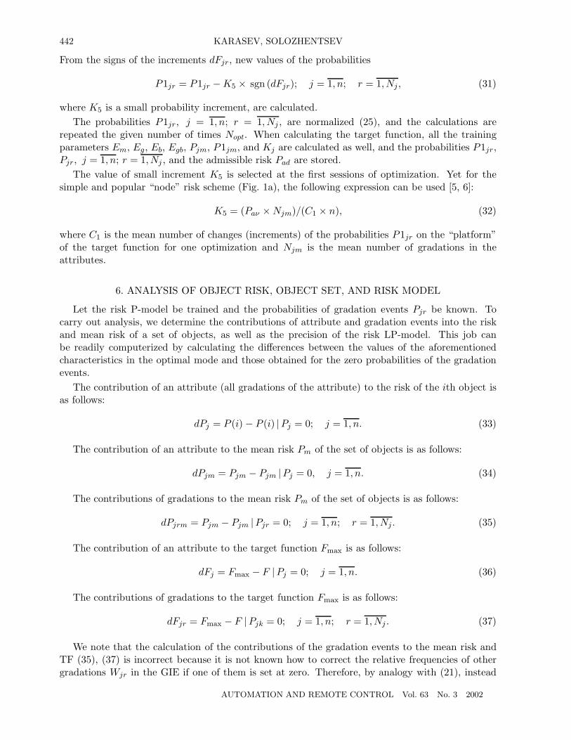
From the signs of the increments dFjr, new values of the probabilities
P1jr = P1jr −K5 × sgn (dFjr); j = 1, n; r = 1, Nj , (31)
where K5 is a small probability increment, are calculated.The probabilities P1jr, j = 1, n; r = 1, Nj , are normalized (25), and the calculations are
repeated the given number of times Nopt. When calculating the target function, all the trainingparameters Em, Eg, Eb, Egb, Pjm, P1jm, and Kj are calculated as well, and the probabilities P1jr,Pjr, j = 1, n; r = 1, Nj , and the admissible risk Pad are stored.
The value of small increment K5 is selected at the first sessions of optimization. Yet for thesimple and popular “node” risk scheme (Fig. 1a), the following expression can be used [5, 6]:
K5 = (Paν ×Njm)/(C1 × n), (32)
where C1 is the mean number of changes (increments) of the probabilities P1jr on the “platform”of the target function for one optimization and Njm is the mean number of gradations in theattributes.
6. ANALYSIS OF OBJECT RISK, OBJECT SET, AND RISK MODEL
Let the risk P-model be trained and the probabilities of gradation events Pjr be known. Tocarry out analysis, we determine the contributions of attribute and gradation events into the riskand mean risk of a set of objects, as well as the precision of the risk LP-model. This job canbe readily computerized by calculating the differences between the values of the aforementionedcharacteristics in the optimal mode and those obtained for the zero probabilities of the gradationevents.
The contribution of an attribute (all gradations of the attribute) to the risk of the ith object isas follows:
dPj = P (i) − P (i) |Pj = 0; j = 1, n. (33)
The contribution of an attribute to the mean risk Pm of the set of objects is as follows:
dPjm = Pjm − Pjm |Pj = 0, j = 1, n. (34)
The contributions of gradations to the mean risk Pm of the set of objects is as follows:
dPjrm = Pjm − Pjm |Pjr = 0; j = 1, n; r = 1, Nj . (35)
The contribution of an attribute to the target function Fmax is as follows:
dFj = Fmax − F |Pj = 0; j = 1, n. (36)
The contributions of gradations to the target function Fmax is as follows:
dFjr = Fmax − F |Pjk = 0; j = 1, n; r = 1, Nj . (37)
We note that the calculation of the contributions of the gradation events to the mean risk andTF (35), (37) is incorrect because it is not known how to correct the relative frequencies of othergradations Wjr in the GIE if one of them is set at zero. Therefore, by analogy with (21), instead
AUTOMATION AND REMOTE CONTROL Vol. 63 No. 3 2002
IDENTIFICATION OF THE LOGICAL-AND-PROBABILISTIC RISK MODELS 443
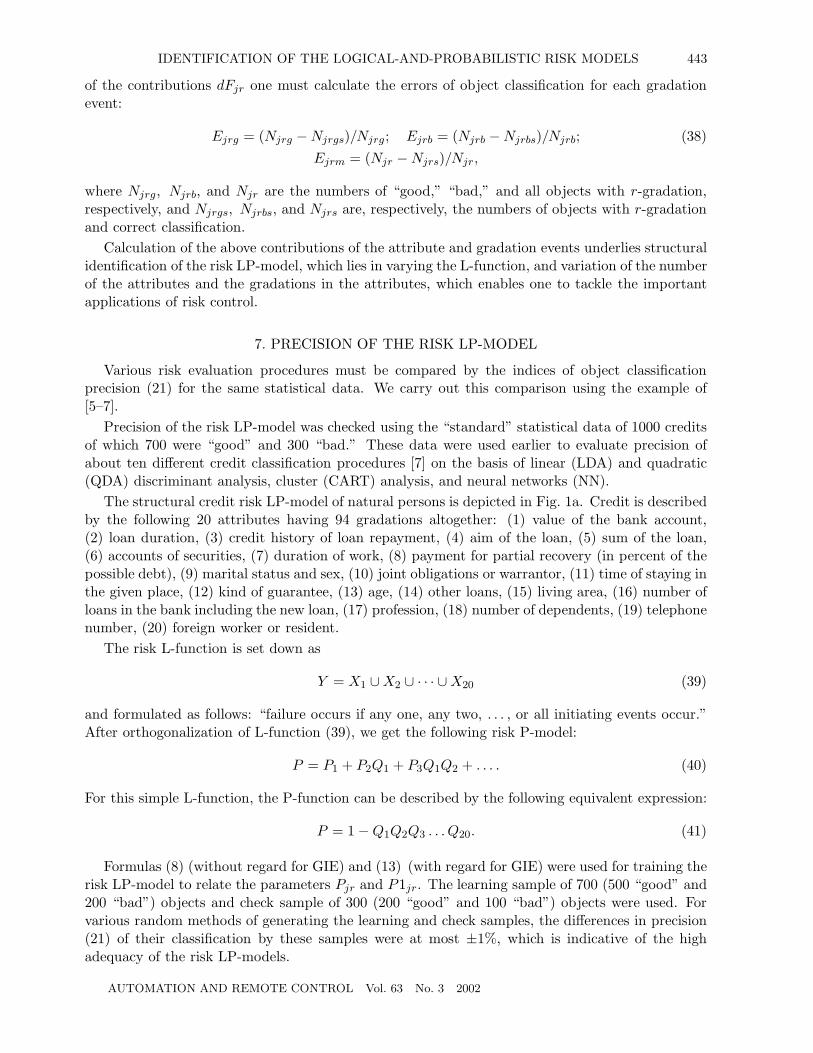
of the contributions dFjr one must calculate the errors of object classification for each gradationevent:
Ejrg = (Njrg −Njrgs)/Njrg; Ejrb = (Njrb −Njrbs)/Njrb; (38)Ejrm = (Njr −Njrs)/Njr,
where Njrg, Njrb, and Njr are the numbers of “good,” “bad,” and all objects with r-gradation,respectively, and Njrgs, Njrbs, and Njrs are, respectively, the numbers of objects with r-gradationand correct classification.
Calculation of the above contributions of the attribute and gradation events underlies structuralidentification of the risk LP-model, which lies in varying the L-function, and variation of the numberof the attributes and the gradations in the attributes, which enables one to tackle the importantapplications of risk control.
7. PRECISION OF THE RISK LP-MODEL
Various risk evaluation procedures must be compared by the indices of object classificationprecision (21) for the same statistical data. We carry out this comparison using the example of[5–7].
Precision of the risk LP-model was checked using the “standard” statistical data of 1000 creditsof which 700 were “good” and 300 “bad.” These data were used earlier to evaluate precision ofabout ten different credit classification procedures [7] on the basis of linear (LDA) and quadratic(QDA) discriminant analysis, cluster (CART) analysis, and neural networks (NN).
The structural credit risk LP-model of natural persons is depicted in Fig. 1a. Credit is describedby the following 20 attributes having 94 gradations altogether: (1) value of the bank account,(2) loan duration, (3) credit history of loan repayment, (4) aim of the loan, (5) sum of the loan,(6) accounts of securities, (7) duration of work, (8) payment for partial recovery (in percent of thepossible debt), (9) marital status and sex, (10) joint obligations or warrantor, (11) time of staying inthe given place, (12) kind of guarantee, (13) age, (14) other loans, (15) living area, (16) number ofloans in the bank including the new loan, (17) profession, (18) number of dependents, (19) telephonenumber, (20) foreign worker or resident.
The risk L-function is set down as
Y = X1 ∪X2 ∪ · · · ∪X20 (39)
and formulated as follows: “failure occurs if any one, any two, . . . , or all initiating events occur.”After orthogonalization of L-function (39), we get the following risk P-model:
P = P1 + P2Q1 + P3Q1Q2 + . . . . (40)
For this simple L-function, the P-function can be described by the following equivalent expression:
P = 1−Q1Q2Q3 . . . Q20. (41)
Formulas (8) (without regard for GIE) and (13) (with regard for GIE) were used for training therisk LP-model to relate the parameters Pjr and P1jr. The learning sample of 700 (500 “good” and200 “bad”) objects and check sample of 300 (200 “good” and 100 “bad”) objects were used. Forvarious random methods of generating the learning and check samples, the differences in precision(21) of their classification by these samples were at most ±1%, which is indicative of the highadequacy of the risk LP-models.
AUTOMATION AND REMOTE CONTROL Vol. 63 No. 3 2002
444 KARASEV, SOLOZHENTSEV
Table 3. Characteristics of object classification by different methodsError Eb of Error Eg of Mean error,
Method used classifying classifying Em“bad” objects “good” objects
LDA Resubstitution 0.2600 0.279 0.273LDA Leaving-one-out 0.2870 0.291 0.290QDA Resubstitution 0.1830 0.283 0.253QDA Leaving-one-out 0.2830 0.340 0.323CART 0.2730 0.289 0.285Neural Network NN1 0.3800 0.240 0.282Neural Network NN2 0.2400 0.312 0.290LP-model without regard for the GIE—Var. 1 0.1670 0.201 0.191LP-model with regard for the GIE—Var. 2 0.1433 0.190 0.176LP-model with regard for the GIE after 0.1260 0.174 0.155structural identification—Var. 3
In contrast to the recognition and classification theory, the identification theory makes use ofanother approach to estimating the adequacy of models based on the statistical data. It determinesefficiency, consistency, and unbiasedness of the estimates of the parameters of the constructedmodel. Some studies that were done in [5] attest to high and controllable adequacy of the riskLP-model. It seems that the test sample is not required for the risk LP-models, which allows oneto improve precision of the risk LP-model by using more information in the learning sample.
With regard for the GIE, the risk LP-model (Table 3, Var. 2) has the following characteristicsafter training: Fmax = 824; Ngs = 567; Nbs = 257; Egb = 3.05; minimum risk Pmin = 0.230;maximum risk Pmax = 0.379; admissible risk Pad = 0.306; and number of independent variables(probabilities) Nind = 74. This risk LP-model has much smaller object classification errors Em =0.176, Eg = 0.190, and Eb = 0.1433 as compared with the existing Western methods whereFmax = 750− 720 and Em = 0.25 − 0.28 [6, 7].
Without regard for the GIE, the risk LP-model (Table 3, Var. 1) after training has the followingcharacteristics: Fmax = 809 and Nind = 94. This risk LP-model has worse classification precision.Importantly, the risk LP-model without regard for the GIE has mush lower stability in objectclassification.
Precision comparison of different procedures based on the same statistical data demonstrated(Table 3) that with regard for the GIE the risk LP-model is almost twice as precise as the objectclassification methods based on the discriminant analysis and neural networks.
Analysis and structural identification (Var. 3, Table 3) even more improve precision of the riskLP-model. As the result, the following decisions can be made: change the size of the gradationintervals; choose the optimal number of attribute gradations; or eliminate some attributes. Thefollowing trend was established for varying number of attribute gradations: the more gradations,the more precise the risk LP-model (the value of the target function Fmax). For example, for theattribute of credit duration, the trend was as follows: 0 gradations (no attribute)—Fmax = 800; 2gradations—Fmax = 814; 4 gradations—Fmax = 822; 10 gradations (initial variant)—Fmax = 824;and 32 gradations—Fmax = 828.
The risk model cannot be absolutely adequate. There exists no algorithm to construct the surfaceseparating the “good” and “bad” objects. It is impossible to prove in mathematical terms whichmethod is superior or inferior to the rest of the methods. One can do this only through examplesusing the same statistical data for training different models. However, it is mathematically evidentthat the probabilistic risk polynomial is much more complex than the equation of plane or convexseparating surface in the discriminant analysis-based methods and is organized much better owingto the GIE than the weighed polynomial in the neural networks.
AUTOMATION AND REMOTE CONTROL Vol. 63 No. 3 2002
IDENTIFICATION OF THE LOGICAL-AND-PROBABILISTIC RISK MODELS 445
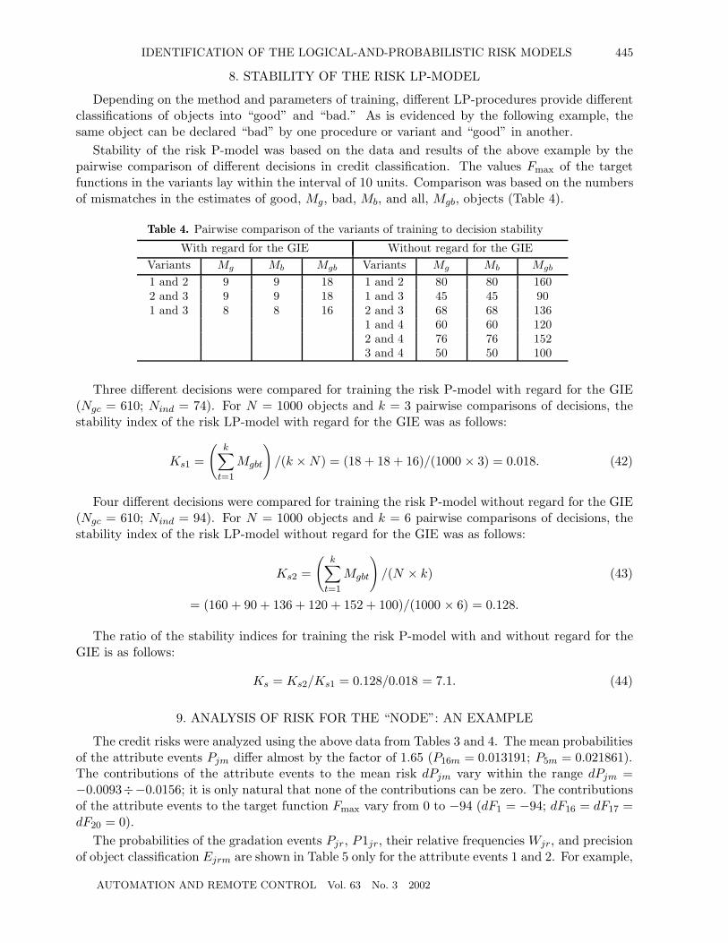
8. STABILITY OF THE RISK LP-MODEL
Depending on the method and parameters of training, different LP-procedures provide differentclassifications of objects into “good” and “bad.” As is evidenced by the following example, thesame object can be declared “bad” by one procedure or variant and “good” in another.
Stability of the risk P-model was based on the data and results of the above example by thepairwise comparison of different decisions in credit classification. The values Fmax of the targetfunctions in the variants lay within the interval of 10 units. Comparison was based on the numbersof mismatches in the estimates of good, Mg, bad, Mb, and all, Mgb, objects (Table 4).
Table 4. Pairwise comparison of the variants of training to decision stability
With regard for the GIE Without regard for the GIEVariants Mg Mb Mgb Variants Mg Mb Mgb
1 and 2 9 9 18 1 and 2 80 80 1602 and 3 9 9 18 1 and 3 45 45 901 and 3 8 8 16 2 and 3 68 68 136
1 and 4 60 60 1202 and 4 76 76 1523 and 4 50 50 100
Three different decisions were compared for training the risk P-model with regard for the GIE(Ngc = 610; Nind = 74). For N = 1000 objects and k = 3 pairwise comparisons of decisions, thestability index of the risk LP-model with regard for the GIE was as follows:
Ks1 =
(k∑t=1
Mgbt
)/(k ×N) = (18 + 18 + 16)/(1000 × 3) = 0.018. (42)
Four different decisions were compared for training the risk P-model without regard for the GIE(Ngc = 610; Nind = 94). For N = 1000 objects and k = 6 pairwise comparisons of decisions, thestability index of the risk LP-model without regard for the GIE was as follows:
Ks2 =
(k∑t=1
Mgbt
)/(N × k) (43)
= (160 + 90 + 136 + 120 + 152 + 100)/(1000 × 6) = 0.128.
The ratio of the stability indices for training the risk P-model with and without regard for theGIE is as follows:
Ks = Ks2/Ks1 = 0.128/0.018 = 7.1. (44)
9. ANALYSIS OF RISK FOR THE “NODE”: AN EXAMPLE
The credit risks were analyzed using the above data from Tables 3 and 4. The mean probabilitiesof the attribute events Pjm differ almost by the factor of 1.65 (P16m = 0.013191; P5m = 0.021861).The contributions of the attribute events to the mean risk dPjm vary within the range dPjm =−0.0093÷−0.0156; it is only natural that none of the contributions can be zero. The contributionsof the attribute events to the target function Fmax vary from 0 to −94 (dF1 = −94; dF16 = dF17 =dF20 = 0).
The probabilities of the gradation events Pjr, P1jr, their relative frequencies Wjr, and precisionof object classification Ejrm are shown in Table 5 only for the attribute events 1 and 2. For example,
AUTOMATION AND REMOTE CONTROL Vol. 63 No. 3 2002
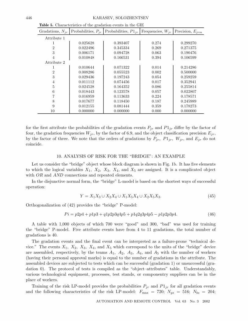
446 KARASEV, SOLOZHENTSEV
Table 5. Characteristics of the gradation events in the GIE
Gradations, Njr Probabilities, Pjr Probabilities, P1jr Frequencies, Wjr Precision, Ejrm
Attribute 11 0.025628 0.393407 0.274 0.2992702 0.022496 0.345334 0.269 0.2713753 0.006171 0.094728 0.063 0.1904764 0.010848 0.166531 0.394 0.106599
Attribute 21 0.010644 0.071322 0.014 0.2142862 0.008286 0.055523 0.002 0.5000003 0.029436 0.197243 0.054 0.2592594 0.011112 0.074456 0.017 0.3529415 0.024528 0.164352 0.086 0.2558146 0.018443 0.123578 0.057 0.0228077 0.016959 0.113633 0.224 0.1785718 0.017677 0.118450 0.187 0.2459899 0.012155 0.081444 0.359 0.178273
10 0.000000 0.000000 0.000 0.000000
for the first attribute the probabilities of the gradation events Pjr and P1jr differ by the factor offour, the gradation frequencies Wjr, by the factor of 6.9, and the object classification precision Ejr,by the factor of three. We note that the orders of gradations by Pjr, P1jr, Wjr, and Ejr do notcoincide.
10. ANALYSIS OF RISK FOR THE “BRIDGE”: AN EXAMPLE
Let us consider the “bridge” object whose block diagram is shown in Fig. 1b. It has five elementsto which the logical variables X1, X2, X3, X4, and X5 are assigned. It is a complicated objectwith OR and AND connections and repeated elements.
In the disjunctive normal form, the “bridge” L-model is based on the shortest ways of successfuloperation:
Y = X1X3 ∪X2X4 ∪X1X5X4 ∪X2X5X3. (45)
Orthogonalization of (42) provides the “bridge” P-model:
Pi = p2p4 + p1p3 + q1p2p3q4p5 + p1q2q3p4p5− p1p2p3p4. (46)
A table with 1,000 objects of which 700 were “good” and 300, “bad” was used for trainingthe “bridge” P-model. Five attribute events have from 4 to 11 gradations, the total number ofgradations is 40.
The gradation events and the final event can be interpreted as a failure-prone “technical de-vice.” The events X1, X2, X3, X4, and X5 which correspond to the units of the “bridge” deviceare assembled, respectively, by the teams A1, A2, A3, A4, and A5 with the number of workers(having their personal approval marks) is equal to the number of gradations in the attribute. Theassembled devices are subjected to tests which can be successful (gradation 1) or unsuccessful (gra-dation 0). The protocol of tests is compiled as the “object–attributes” table. Understandably,various technological equipment, processes, test stands, or componentry suppliers can be in theplace of workers.
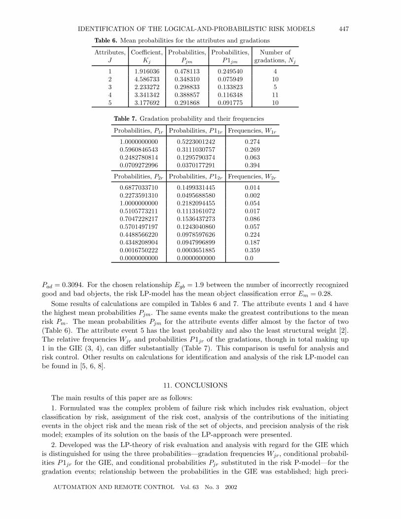
Training of the risk LP-model provides the probabilities Pjr and P1jr for all gradation eventsand the following characteristics of the risk LP-model: Fmax = 720; Ngs = 516; Nbs = 204;
AUTOMATION AND REMOTE CONTROL Vol. 63 No. 3 2002
IDENTIFICATION OF THE LOGICAL-AND-PROBABILISTIC RISK MODELS 447
Table 6. Mean probabilities for the attributes and gradations
Attributes, Coefficient, Probabilities, Probabilities, Number ofJ Kj Pjm P1jm gradations, Nj
1 1.916036 0.478113 0.249540 42 4.586733 0.348310 0.075949 103 2.233272 0.298833 0.133823 54 3.341342 0.388857 0.116348 115 3.177692 0.291868 0.091775 10
Table 7. Gradation probability and their frequencies
Probabilities, P1r Probabilities, P11r Frequencies, W1r
1.0000000000 0.5223001242 0.2740.5960846543 0.3111030757 0.2690.2482780814 0.1295790374 0.0630.0709272996 0.0370177291 0.394
Probabilities, P2r Probabilities, P12r Frequencies, W2r
0.6877033710 0.1499331445 0.0140.2273591310 0.0495688580 0.0021.0000000000 0.2182094455 0.0540.5105773211 0.1113161072 0.0170.7047228217 0.1536437273 0.0860.5701497197 0.1243040860 0.0570.4488566220 0.0978597626 0.2240.4348208904 0.0947996899 0.1870.0016750222 0.0003651885 0.3590.0000000000 0.0000000000 0.0
Pad = 0.3094. For the chosen relationship Egb = 1.9 between the number of incorrectly recognizedgood and bad objects, the risk LP-model has the mean object classification error Em = 0.28.
Some results of calculations are compiled in Tables 6 and 7. The attribute events 1 and 4 havethe highest mean probabilities Pjm. The same events make the greatest contributions to the meanrisk Pm. The mean probabilities Pjm for the attribute events differ almost by the factor of two(Table 6). The attribute event 5 has the least probability and also the least structural weight [2].The relative frequencies Wjr and probabilities P1jr of the gradations, though in total making up1 in the GIE (3, 4), can differ substantially (Table 7). This comparison is useful for analysis andrisk control. Other results on calculations for identification and analysis of the risk LP-model canbe found in [5, 6, 8].
11. CONCLUSIONS
The main results of this paper are as follows:1. Formulated was the complex problem of failure risk which includes risk evaluation, object
classification by risk, assignment of the risk cost, analysis of the contributions of the initiatingevents in the object risk and the mean risk of the set of objects, and precision analysis of the riskmodel; examples of its solution on the basis of the LP-approach were presented.
2. Developed was the LP-theory of risk evaluation and analysis with regard for the GIE whichis distinguished for using the three probabilities—gradation frequencies Wjr, conditional probabil-ities P1jr for the GIE, and conditional probabilities Pjr substituted in the risk P-model—for thegradation events; relationship between the probabilities in the GIE was established; high preci-
AUTOMATION AND REMOTE CONTROL Vol. 63 No. 3 2002
448 KARASEV, SOLOZHENTSEV
sion and stability of the risk LP-model based on the GIE (Bayes formulas) and well-organized riskpolynomial was substantiated.
3. Formulated was the problem of identification of the risk LP-model from the statistical data;an algorithm to solve it was proposed; and methods of identification of the risk P-model based onrandom search and small probability increments by the sign of variation of the target function weredeveloped.
4. Examples of training and analyzing the risk LP-models of different logical complexities werepresented. They demonstrated that the risk LP-models have twice as high precision and seven-foldstability of object classification as compared with the methods based on discriminant analysis andneural networks.
REFERENCES
1. Aven, T. and Jensen, U., Stochastic Models in Reliability, New York: Springer, 1999.
2. Ryabinin, I.A. and Cherkessov, G.N., Logiko-veroyatnostnyi metod issledovaniya nadezhnosti strukturno-slozhnykh sistem (Logical-and-Probabilistic Method of Studying Structurally Complex Systems), Moscow:Radio i Svyaz’, 1981.
3. Henly, E.I. and Kumamoto, H., Reliability Engineering and Risk Assessment, New York: Prentice Hall,1985.
4. Volik, B.G. and Ryabinin, I.A., Control Systems: Efficiency, Reliability, and Survivability, Avtom. Tele-mekh., 1984, no. 12, pp. 151–160.
5. Solozhentsev, E.D., Karasev, V.V., and Solozhentsev, V.E., Logiko-veroyatnostnye modeli riska v bankakh,biznese i kachestve (Logical-and-Probabilistic Risk Models in Banks, Business, and Quality), St. Peters-burg: Nauka, 1999.
6. Solojentsev, E.D. and Karasev, V.V., Risk Logic and Probabilistic Models in Business and Identificationof Risk Models, Informatica, 2001, vol. 25, pp. 49–55.
7. Seitz, J. and Stickel, E., Consumer Loan Analysis Using Neural Network. Adaptive Intelligent Systems,in Proc. Bankai Workshop, Brussels: Elsevier, 1993, pp. 177–192.
8. Solozhentsev, E.D., Parametrical and Structural Identification of the Logical-and-Probabilistic Risk Mod-els in Banks, Business, and Quality, Int. Conf. “System Identification and Control Problems,” Moscow,2000.
This paper was recommended for publication by B.G. Volik, a member of the Editorial Board
AUTOMATION AND REMOTE CONTROL Vol. 63 No. 3 2002


![NeoPHOX a structurally tunable ligand system for ... · PDF fileNeoPHOX – a structurally tunable ligand ... [4-12]. One of the major areas of application ... NeoPHOX a structurally](https://img.pdfslide.net/doc/110x75/5aba21307f8b9af27d8b514a/neophox-a-structurally-tunable-ligand-system-for-a-structurally-tunable.jpg)