Embed Size (px)
Citation preview
Chapter 1
IMAGE COMPRESSION USING SPLINEBASED WAVELET TRANSFORMS
Amir Z. AverbuchSchool of Computer Science, Tel Aviv UniversityTel Aviv 69978, [email protected]
Valery A. ZheludevSchool of Computer Science, Tel Aviv UniversityTel Aviv 69978, [email protected]
Abstract In paper we describe a successful applications of the wavelet transformsto still image compression. The wavelet transforms were designed bythe usage of discrete interpolatory splines. These filters outperform thetraditional biorthogonal 9/7 filters which are frequenty used in waveletbased compression. The new filters and the biorthogonal 9/7 are incor-porated into SPIHT in order to measure and compare their performancewith one well known codec.
Keywords: Sample, edited book
IntroductionThe three fundamental building blocks of compression systems, are
transformation (such as Discrete Cosine Transform, wavelets), quanti-zation (SQ, UTQ, etc.), and symbol modeling and encoding (Huffman,and arithmetic). In this paper we present new wavelet based filterswhich have good performance for still image compression and outper-forms the traditional biorthogonal 9/7 filters which are frequenty usedin wavelet based compression. The new filters and the biorthogonal 9/7
1
2
are incorporated into SPIHT [34] in order to measure and compare theirperformance with one well known codec.
0.1. Wavelet Based Image CodersWavelet transforms provide very good energy compaction: the trans-
form decreases the correlation between the transformed coefficients. Eventhough the correlation between wavelet coefficients across scale is verysmall, the coefficients are not independent (there is no contradiction,since the probability density function of wavelet coefficients of naturalimage are not Gaussian). In fact, a visual inspection of the wavelet co-efficients of an image will reveal that there are still coherent structuresin the higher frequency bands. Furthermore these structures have a selfsimilar structure across the different subbands.
While the wavelet coders are based on the wavelet decomposition andits multiresolution, the JPEG is based on 8×8 windowed Fourier trans-form. Therefore, JPEG ignores correlations among pixels over largerareas. This causes “blocking” effect in deep compression. Also, whilethe DCT-based image coders perform very well at moderate bit rates, athigher compression ratios image quality degrades because of the artifactsresulting from the block-based DCT scheme. Wavelet-based coding onthe other hand provides substantial improvement in picture quality atlow bit rates. Because of the inherent multiresolution nature, wavelet-based coders facilitate progressive transmission of images thereby allow-ing variable bit rates.
Over the past few years, a variety of novel and sophisticated wavelet-based image coding schemes have been developed. A family of al-gorithms, known as zerotree coders, exploit both the inter-band self-similarity, as well as the intraband coherent structure, and the depen-dencies across subbands. These include wavelet codecs ([2, 5, 6, 24, 3]),Embedded Zero Tree Wavelet (EZW) [36], Set Partitioning in Hierar-chical Trees (SPIHT) [34], which uses the 9-7 biorthogonal filters [21],instead of the 9 tap filters of [1]), Space-Frequency Quantization forWavelet Image Coding (SFQ) [44], which addresses the problem of howspatial quantization modes and standard scalar quantization can be ap-plied in a jointly optimal fashion in an image coder, Efficient Pre-CodingTechniques for Wavelet-Based Image Compression (PACC) [29], intro-duces a coding method using a fast wavelet transform and an uniformquantizer combined with a framework of preceding techniques whichare based on the concepts of partitioning, aggregation and conditionalcoding- PACC. Following these concepts, the data object emerging fromthe quantizer is first partitioned into different subsources. Parts of cor-
Image compression using spline based wavelet transforms 3
relations within and between different subsources are then captured byaggregating homogeneous elements into data structures like run-lengthcodes or zerotrees), EQ[28], (Image Coding Based on Mixture Modelingof Wavelet Coefficients and a Fast Estimation-Quantization Frameworkintroduces an image compression paradigm that combines compressionefficiency with speed, and is based on an independent “infinite” mix-ture model which accurately captures the space-frequency characteri-zation of the wavelet image representation), Morphological Represen-tation of Wavelet Data (MRWD) [35], (presents both an experimentalstudy of the statistics of wavelet data, as well as the design of two differ-ent morphology-based coding algorithms, that make use of these statis-tics), SLCCA[12], (Significance-Linked Connected Component Analy-sis for Wavelet Image Coding, is a wavelet image coder which extendsMRWD by exploiting both within-subband clustering of significant co-efficients and cross-subband dependency in significant fields), ContextBased (C/B)[16], (Context-Based Entropy Coding for Lossy WaveletImage Compression which is an adaptive image coding algorithm basedon backward adaptive quantization-classification techniques using a sim-ple uniform scalar quantizer to quantize the image subbands), OC [26],Optimal Classification in Subband Coding of Images investigates variousclassification techniques, applied to subband coding of images, as a wayof exploiting the non-stationary nature of image subbands), CREW[13],EPWIC[14], EBCOT[38], (Scalable Image Compression which is basedon independent Embedded Block Coding with Optimized Truncation ofthe embedded bit-streams, which identifies some of the major contri-butions of the algorithm. The EBCOT algorithm [38] uses a wavelettransform to generate the subband coefficients which are then quantizedand coded. Although the usual dyadic wavelet decomposition is typi-cal, other “packet” decompositions are also supported and occasionallypreferable), SR([39]), Image Coding using Adaptive Wavelets[41] (thewavelet filter should be chosen adaptively depending on the statisticalnature of image being coded), Second Generation Image Coding[24],Image Coding using Wavelet Packets ([4, 19]), (larger libraries of wave-forms which have been developed in order to describe long oscillatorypatterns. The selected collection of patterns is called the “best basis”.It is demonstrated that, despite this difficulty, the freedom to choose anadapted basis remains an enormous advantage), Wavelet Image Codingusing VQ ([3]), and Lossless Image Compression using Integer Lifting[15], and hybrid codec that combine wavelet and waveletpacket [10] orany other combination.
The emerging standard, called JPEG-2000 [46], is being developed intwo parts and is based upon wavelet decomposition. Combined with
4
powerful quantization and encoding strategies such as embedded quan-tization and context based arithmetic coding, the use of wavelets inJPEG-2000 provides the potential for numerous advantages over the ex-isting JPEG standard. Performance gains include improved compressionefficiency at low bit rates or for large images, while new functionalitiesinclude multi-resolution representation, SNR scalability and embeddedbit stream architecture, lossy to lossless progression, region-of-interest(ROI) coding, and a rich file format, random access and processing ofseparate parts of picture, robustness to bit errors, open architecture,content based description and interface with MPEG-4 [47].
0.2. Usage of splines for wavelet designBy now two ways were pursued for the construction of wavelet schemes
via the usage of splines. One is to construct orthogonal and semi-orthogonal wavelets in the spline spaces (Battle-Lemarie [11, 27], Chui-Wang [17], Unser-Aldroubi-Eden [40]), Zheludev [45]. Another way wasintroduced by Cohen, Daubechies and Feauveau [20] who constructedsymmetric compactly supported spline wavelets whose duals, remainingcompactly supported and symmetric, do not belong to a spline space.However, since the introduction of the lifting scheme for the design ofwavelet transforms [37], a new way was opened to use splines as a toolfor devising a full discrete scheme of wavelet transforms.
The basic lifting scheme for wavelet transform of a discrete -timesignal x consists of three steps:
Split – The signal is split into even and odd subarrays: s = {s(k) =x(2k)}, d = {d(k) = x(2k + 1)}, k ∈ Z.
Predict - Some linear combinations of terms of the even array s areused to predict the odd array d . Then, the array d is redefined asthe difference between the existing array and the predicted one. Ifthe predictor is chosen correctly, this step decorrelates the signaland reveals its high-frequency component.
Update – To eliminate aliasing, which appears while downsamplingthe original signal x into s and, by this means, to obtain the low-frequency component of the signal, the even array is updated usingthe new odd array.
The newly produced even and odd subarrays are the coefficients ofone decomposition step of a wavelet transform s (low-frequency) andd (high-frequency). The inverse transform is implemented in a reverseorder. The transform generates biorthogonal wavelet bases for the signal
Image compression using spline based wavelet transforms 5
space. The specifics of the transform and its generated wavelets aredetermined by the choice of the predicting and updating aggregates.
In the construction by Donoho [23], which later was modified bySweldens [37], an odd sample is predicted from a polynomial interpo-lation of neighboring even samples. Wavelets, which were generated bythese transforms, are symmetric and compactly supported. Since thetransform is interpolating, it operates immediately on the samples ofthe signal. However, these wavelet transforms are not efficient in appli-cations.
New opportunities for design of wavelet transforms become availableby usage of splines instead of polynomials as the predicting and updatingaggregates in the lifting schemes.
Continuous interpolatory splines. The interpolatory spline ofodd order 2m − 1 (even degree) with equidistant nodes possesses a re-markable property of super-convergence in the midpoints of the intervalsbetween grid points k/N [43]. In these points it approximates the smoothfunction f with an accuracy of N−2m whereas the global approximationaccuracy is N−(2m−1). Thus we build the spline of an odd order 2m− 1which interpolates the even samples of the signal x and predict the oddsamples by the values of the spline in the midpoints of the intervals be-tween the grid points. The prediction is exact on the polynomials ofdegrees up to 2m. This leads to the decomposition wavelets with 2m+1vanishing moments. To supply the reconstruction wavelets with similarproperty, the even array can be updated by adding the values in themidpoints between the grid points of the spline, which interpolates thenew odd samples (divided by two). The order of the update spline maydiffer from the order of the spline, which was employed for prediction.This scheme is described in our paper [9].
Discrete interpolatory splines. Another option is to use thediscrete rather than continuous interpolatory splines. We describe thediscrete splines construction in [7, 8]. In this case explicit formulasfor the transforms with any number of vanishing moments are estab-lished. Moreover, our investigation revealed an interesting relation be-tween the discrete splines and the Butterworth filters commonly usedin signal processing. The filter banks, which are used in our scheme,comprise filters which act as a bi-directional half-band Butterworth fil-ters. The frequency response of Butterworth filters are maximally flatand we succeeded in construction of the dual filters with similar prop-erty. Unlike the construction in [23], the designed transforms are usingcausal and anti-causal linear phase filters with infinite impulse response
6
(IIR). However , the transfer functions of the employed filters are ratio-nal. Therefore, filtering can be performed in a recursive manner. Weestablished explicit formulas which enable fast cascade or parallel imple-mentation. The boundaries are handled using symmetric extensions ofthe signals. The one-pass Butterworth filters were used already for de-vising orthogonal non-symmetric wavelets [25]. The computations therewere conducted in time domain using recursive filtering. A scheme usingrecursive filters for the construction of biorthogonal symmetric waveletswas presented in [32], [30].
In the present paper we describe application of the wavelet transformsdesigned with usage of the discrete interpolatory splines to image com-pression. Details of construction and proofs of formulated propositionscan be found in [8]. The rest of the paper is organized as follows. InSection 1 we recall the notion and outline necessary properties of thez-transform, Butterworth filters and interpolatory discrete splines. InSection 2 we introduce a family of biorthogonal wavelet-type transformsof discrete-time signals, which we construct through lifting steps. InSection 3 we interpret devised scheme as a transformation of the signalsby a filter bank that possesses the perfect reconstruction properties. Wereveal relation of this filter bank to Butterworth filters. In Section 3.2we discuss choosing the control filter which is used in the update step.In Section 4 we describe recursive implementation of the transforms.We present general formulas which allow fast cascade or parallel imple-mentation of transforms of any order. Then we give examples of mostpractical filters. The perfect reconstruction filter banks, that were con-structed in previous sections, are associated with the biorthogonal pairsof of wavelet-type bases in the space of discrete-time signals. We de-scribe these bases in Section 5. In Section 6 we explain one multiscaleadvance of the devised wavelet transforms. Section 7 is devoted to thepresenta of results of experiments on image compression using devisedbiorthogonal transforms. In Section 7.1 we describe in details the trans-forms, which we employed in the experiments. In Section 7.2 we discusscomputational complexity of the transforms. In Section 7.3 we presentresults of compression of four well-known benchmark images.
1. Preliminaries
1.1. z-transformThe sequences {a(k)}∞k=−∞, which belong to the space l1, we call the
discrete-time signals. The space of discrete-time signals we denote by S.The z−transform of a signal {a(k)} ∈ S is defined as follows:
Image compression using spline based wavelet transforms 7
a(z) =∞∑
k=−∞z−k a(k).
Throughout the paper we assume that z = eiω. We recall the followingproperties of the z−transform:
a(k) =∞∑
l=−∞b(k − l)c(l) ⇐⇒ a(z) = b(z) c(z)
ae(z2) ∆=∞∑
k=−∞z−2k a(2k) =
12
(a(z) + a(−z))
ao(z2) ∆=∞∑
k=−∞z−2k a(2k + 1) =
z
2(a(z)− a(−z))
a(z) = ae(z2) + z−1ao(z2).
za(z) =∞∑
k=−∞z−k a(k + 1),
that is za(z) is the z−transform of the shifted signal {a(k + 1)}.
1.2. Discrete splinesThe discrete B-spline of the first order is defined by the following
sequence:
B1,n(j) =
{1 if j = 0, . . . , 2n− 1, n ∈N,
0, otherwise, j ∈ Z.
We define the higher order B-splines as the discrete convolutions byrecurrence: Bp,n = B1,n ∗ Bp−1,n. Obviously, the z-transform of the B-spline of order p is
Bp,n(z) = (1 + z−1 + z−2 + . . . + z−2n+1)p p = 1, 2, . . . .
In this paper we are interested only in the case when p = 2r, r ∈ Nand n = 1. The corresponding splines are denoted as Br = B2r,1. Inthis case we have Br(z) = (1 + z−1)2r. The B-spline Br(j) is symmetricabout the point j = r where it attains its maximal value. We define thecentral B-spline Qr(j) of order 2r as a shift of the B-spline:
Qr(j)∆= Br(j + r), Qr(z) = zrBr(z) = zr(1 + z−1)2r.
8
The discrete spline of order 2r is defined as a linear combination, withreal-valued coefficients, of shifts of the central B-spline of order 2r:
Sr(k) ∆=∞∑
l=−∞c(l)Qr(k − 2l).
Definition 1.1 Let {e(k)} ∈ S be a given sequence.The discrete splineSr is called the interpolatory spline if the following relations hold:
Sr(2k) = e(k), k ∈ Z. (1.1)
The points {2k} are called the nodes of the spline.
The following proposition shows how interpolatory splines of anyorder can be constructed. Moreover, for further development we needto know the values of the splines in the midpoints between the nodes,which we denote as σ(k) = Sr(2k + 1), k ∈ Z.
Proposition 1.1 The interpolatory spline which satisfies the condi-tions (1.1) is represented as follows
Sr(k) =∞∑
l=−∞c(l)Qr(k − 2l), c(z2) =
2e(z2)zr (1 + z−1)2r + (−z)r (1− z−1)2r .
The z−transform of the interpolatory spline in the midpoints are
σ(z2) = zUr(z)e(z2), Ur(z) ∆=(1 + z−1
)2r − (−1)r(1− z−1
)2r
(1 + z−1)2r + (−1)r (1− z−1)2r . (1.2)
In addition, Ur(−z) = −Ur(z).
1.3. Discrete-time Butterworth filtersWe recall briefly the notion of Butterworth filter. For details we refer
to [31]. The input x(n) and the output y(n) of a linear discrete timeshift-invariant system are linked as
y(n) =∞∑
k=−∞f(k)x(n− k). (1.3)
Such a processing of the signal x(n) is called digital filtering and the se-quence f(n) is called the impulse response of the filter. Its z−transformf(z) =
∑∞n=−∞ z−nf(n) is called the transfer function of the filter. De-
note by X(ω) =∑∞
n=−∞ e−iωnx(n), Y (ω) =∑∞
n=−∞ e−iωny(n), F (ω) =∑∞n=−∞ e−iωnf(n) the discrete Fourier transforms of the sequences. Then,
Image compression using spline based wavelet transforms 9
we have from (1.3) Y (ω) = F (ω)X(ω). The function F (ω) is called thefrequency response of the digital filter. The digital Butterworth filteris a filter with a maximally flat frequency response. The magnitudesquared frequency responses Fl(ω) and Fh(ω) of the digital low-pass andhigh-pass Butterworth filters of order r, respectively, are given by theformulas
|Fl(ω)|2 =1
1 + (tan ω2 / tan ωc
2 )2r,
|Fh(ω)|2 = 1− |Fl(ω)|2 =1
1 + (tan ωc2 / tan ω
2 )2r
where ωc is the cutoff frequency.We are interested in the half-band Butterworth filters that is ωc =
π/2. In this case
|Fl(ω)|2 =1
1 + (tan ω2 )2r
, |Fh(ω)|2 = 1− |Fl(ω)|2 =1
1 + (cot ω2 )2r
.
If we put z = eiω then we obtain the magnitude squared transfer functionof the low-pass filter:
|fl(z)|2 =(1 + z−1
)2r
(1 + z−1)2r + (−1)r (1− z−1)2r (1.4)
Similarly, we have the magnitude squared transfer function of the high-pass filter:
|fh(z)|2 =(−1)r
(1− z−1
)2r
(1 + z−1)2r + (−1)r (1− z−1)2r (1.5)
It is readily seen that the function Ur defined in (1.2), is related to thesetransfer functions:
1 + Ur(z) = 2|fl(z)|2, 1− Ur(z) = 2|fh(z)|2. (1.6)
2. Biorthogonal transformsWe introduce a family of biorthogonal wavelet-type transforms that
operate on the signal x = {x(k)}∞k=−∞, which we construct throughlifting steps. We carry out the construction in the z− domain and discussthe time-domain implementation in subsequent sections.
The lifting scheme can be implemented in a primal or dual modes. Weconsider only the primal mode because this scheme steadily outperformsthe dual one in image processing applications.
10
2.1. DecompositionGenerally, the primal lifting scheme for decomposition of signals con-
sists of three steps: 1. Split. 2. Predict. 3. Update or lifting. Let usconstruct our proposed schemes in terms of these steps.
Split - We split the array x into an even and odd sub-arrays:
e1 = {e1(k) = x(2k)}, d1 = {d1(k) = x(2k + 1)}, k ∈ Z.
Predict - We use the even array e1 to predict the odd array d1 andredefine the array d1 as the difference between the existing arrayand the predicted one. To be specific, we use the spline Sr whichinterpolates the sequence e1 and predict the function d1(z2) whichis the z2−transform of d1. It is predicted by the function σ(z)defined in (1.2). The z−transform of the new d−array is definedas follows:
du1(z2) = d1(z2)− zUr(z)e1(z2). (1.7)
From now on the superscript u means an update operation of thearray.
Lifting - We update the even array using the new odd array:
eu1(z2) = e1(z2) + β(z)z−1 du
1(z2). (1.8)
Generally, the goal of this step is to eliminate aliasing which ap-pears while downsampling the original signal x into e1. By doingso we have that e1 is transformed into a low-pass filtered and down-sampled replica of x. In Section 3.2 we will discuss how to achievethis effect by a proper choice of the control filter β , but for nowwe only require the function β(z) to be real-valued and obey thecondition β(−z) = −β(z), so the product β(z)z−1 is a function ofz2.
2.2. ReconstructionThe reconstruction of the signal x from the arrays eu
1 and du1 is im-
plemented in reverse order: 1. Undo Lifting. 2. Undo Predict. 3.Unsplit.
Undo Lifting - We restore the even array:
e1(z2) = eu1(z2)− β(z)z−1 du
1(z2). (1.9)
Image compression using spline based wavelet transforms 11
Undo Predict - We restore the odd array:
d1(z2) = du1(z2) + zUr(z)e1(z2). (1.10)
Unsplit - The last step represents the standard restoration of the sig-nal from its even and odd components. In the z− domain it looksas:
x(z) = e1(z2) + z−1d1(z2). (1.11)
3. Filter banks
3.1. Relation to Butterworth filtersLifting schemes, that were presented above, yield efficient algorithms
for the implementation of the forward and backward transform of x ←→eu1 ∪ du
1 . But these operations can be interpreted as transformations ofthe signals by a filter bank that possesses the perfect reconstructionproperties.
First we define two filter transfer functions
Φl,r(z) ∆= (1 + Ur(z))/2, Φh,r(z) ∆= (1− Ur(z))/2. (1.12)
¿From (1.6) it is clear that the linear phase filter with the transfer func-tion Φl,r(z) is equal to the magnitude squared transfer function of thediscrete-time low-pass half-band Butterworth filter of order r. The linearphase filter with the transfer function Φh,r(z) is equal to the magnitudesquared transfer function of the high-pass half-band Butterworth filter.It means that application of these filters on a signal is equivalent totwo passes applications (causal and anti-causal) of the correspondingButterworth filters. We call these filters the bi-directional Butterworthfilters.
Define the filter functions
gr(z) ∆= 2z−1Φh,r(z), hrβ(z) ∆= 1 + 2β(z)Φh,r(z) = 1 + β(z) zgr(z),
(1.13)
hr(j) ∆= 2Φl,r(z) grβ(z) ∆= z−1 (1− 2β(z)Φl,r(z)) = z−1 (1− β(z) hr(z)) .
(1.14)We call hr
β(z) and gr(z) the transfer functions of the low-pass and high-pass primal decomposition filters, respectively. We call hr(z) and gr
β(j)
12
the transfer functions of the low-pass and high-pass primal reconstruc-tion filters, respectively. These four filters form a perfect reconstructionfilter bank ([42]).
Theorem 1 The decomposition and reconstruction formulas can be rep-resented as follows:
eu1(z2) =
12
(hr
β(z) x(z) + hrβ(−z) x(−z)
)(1.15)
du1(z2) =
12
(gr(z) x(z) + gr(−z) x(−z)
)(1.16)
x(z) = hr(z)eu1(z2) + gr
β(z) du1(z2). (1.17)
If β(−z) = −β(z) then the functions hrβ(j), gr(j), hr(j) and gr
β(j)satisfy the perfect reconstruction conditions
hr(z) hrβ(z) + gr
β(z) gr(z) = 2
hr(z) hrβ(−z) + gr
β(z) gr(−z) = 0. (1.18)
The following is an obvious observation.
Proposition 3.1 The filter functions are linked to each other in thefollowing way:
gr(z) = z−1hr(−z); grβ(z) = z−1 hr
β(−z)
Remark . We notice that the reconstruction filter hr(z) is equal(up to constant factors) to the transfer function of the bi-directional low-pass half-band Butterworth filter of order r. The decomposition filtergr(z) multiplied by z is equal to the bi-directional high-pass half-bandButterworth filter.
3.2. Choosing the control filterSo far we did not specify how to choose the filter β, which occurs
during the construction of the primal filters grβ and hr
β and the dual onesGR
β and HRβ . The only imposed requirements were that the function
β(z) be real-valued and β(−z) = −β(z). Therefore, we are free to usethe function β1 for custom design of these filters and the correspondingwavelets. We consider here only one approach how to choose the controlfilter β(j) which results in retaining the maximal flatness of the filters.
As was mentioned above, the reconstruction filter hr and the decom-position filter gr are equal to the bi-directional low- and high-pass half-band Butterworth filters of order r, Φl,r and Φh,r, respectively. These
Image compression using spline based wavelet transforms 13
filters are linear phase and maximally flat in their pass- and stop-bandsdue to the factors
(1 + z−1
)2r for the low-pass filters and(1− z−1
)2r
for the high-pass filters (see(1.4) (1.5)). Moreover, since Φh,r(z) hasroot of order 2r at z = 1, filtering with Φh,r eliminates discrete poly-nomials up to degree 2r − 1. Consequently, the corresponding analysiswavelets have 2r vanishing moments (we will discuss this in Section 5.)The low-pass transfer function linked to the high-pass one as follows:Φl,r(z) = 1− Φh,r(z). Thus, filtering with Φl,r restores discrete polyno-mials up to degree 2r − 1. We retain similar properties for filters whichdepend on β: hr
β and grβ. To achieve it, we choose for filters of order r:
β(z) = Up(z)/2 = Φl,p(z)− 12
=12− Φh,p(z). (1.19)
Proposition 3.2 If filter β is chosen as in (1.19), where p is a naturalnumber, then the analysis filter hr
β restores discrete polynomials up todegree 2r − 1 and the synthesis filter gr
β eliminates discrete polynomialsup to degree 2q − 1, where q = min{p, r}.
Proof: Consider first the analysis filter
hrβ(z) = 1 +
12Up(z)
(1− Ur(z)
)= 1 + Φh,r(z)− 2Φh,p(z)Φh,r(z).
Since Φh,r eliminates polynomials up to degree 2r− 1, it is clear that hrβ
restores such polynomials. Similarly
grβ(z) = z−1
(1− 1
2Up(z)
(1 + Ur(z)
))
= z−1 [Φh,r(z) + 2Φh,p(z)− 2Φh,p(z)Φh,r(z)] .
We mark the special case when p = r. Then
hβ(z) = Φl,r(z)(1 + 2Φh,r(z))
gβ(z) = z−1 [Φh,r(z)(1 + 2Φl,r(z))] .
We see that, as in the case of the filters hr and gr, the filters hrβ and gr
βare also mirrored replicas of each other. They differ from bi-directionalButterworth filters of order r by the term 2Φl,r(z)Φh,r(z) which affectsonly the central part of the frequency domain.
14
4. Recursive implementation of the transforms
4.1. General formulasOnce we have chosen the control filter β as in (1.19), the decomposi-
tion procedure is the following (see (1.7), (1.8)):
du1(z2) = d1(z2)− zUr(z)e1(z2) (1.20)
eu1(z2) = e1(z2) +
12z−1Up(z) du
1(z2). (1.21)
The transfer function z−1Up(z)/2 differs from zUp(z)/2 only by the fac-tor z−2 that is the impulse responses of the corresponding filters areidentical up to a shift. Thus both operations of the decomposition are,in principle, identical. For the reconstruction the same operation areconducted in a reverse order.
Therefore, it is sufficient to describe implementation of filtering withthe function zUr(z). From (1.2) one can see that the function zUr(z)depends actually on z2 and we denote it as
Fr(z2) ∆= zUr(z) = z(1 + z)2r − (−1)r (z − 1)2r
(1 + z)2r + (−1)r (z − 1)2r . (1.22)
We introduce a few notation. We distinguish between two cases.
Odd case: Let r = 2q + 1. Then we denote for k = 1, . . . , q :
αrk = cot2
(q + k)π2r
< 1, γrk = cot2
(2q + 2k + 1)π4r
< 1 (1.23)
Even case: Let r = 2q. Then we denote for k = 1, . . . , q :
αrk = cot2
(2q + 2k − 1)π4r
< 1, γrk = cot2
(q + k)π2r
< 1. (1.24)
Proposition 4.1 If r = 2q + 1 then the function Fr(z) is representedas follows:
Fr(z) =αr
1αr2 . . . αr
q(1 + z)∏q
k=1(1 + γrkz−1)(1 + γr
kz)2rγr
1γr2 . . . γr
q
∏qk=1(1 + αr
kz−1)(1 + αr
kz)
= Ar(1 + z)q∏
k=1
Rr(z, k)q∏
k=1
Rr(z−1, k) where (1.25)
Ar∆=
αr1α
r2 . . . αr
q
2rγr1γ
r2 . . . γr
q
, Rr(z, k) ∆=1 + γr
kz
1 + αrkz
.
Image compression using spline based wavelet transforms 15
If r = 2q then
Fr(z) =2rαr
1αr2 . . . αr
q(1 + z)∏q−1
k=1(1 + γrkz−1)(1 + γr
kz)γr
1γr2 . . . γr
q−1
∏qk=1(1 + αr
kz−1)(1 + αr
kz)
= Ar(1 + z)q∏
k=1
Rr(z, k)q∏
k=1
Rr(z−1, k), where (1.26)
Ar∆=
2rαr1α
r2 . . . αr
q
γr1γ
r2 . . . γr
q−1
, Rr(z, q) ∆=1
1 + αrqz
, Rr(z, k) ∆=1 + γr
kz
1 + αrkz
,
k = 1, . . . , q − 1.
To illustrate the implementation we consider the primal decomposi-tion procedure. Since zU(z) = Fr(z2) then the decomposition formulas(1.20), and (1.21) are equivalent to the following
du1(z) = d1(z)− Fr(z)e1(z) (1.27)
eu1(z) = e1(z) +
12z
Fp(z) du1(z). (1.28)
Equation (1.27) means that in order to obtain the detail array du1 , we
must process the even array e1 by the filter Fr with the transfer functionFr(z) and extract the filtered array from the odd array d1. Equation(1.28) means that in order to obtain the smoothed array eu
1 , we mustprocess the detail array du
1 by the filter Φr that has the transfer functionΦr(z) = z−1Fr(z)/2 and add the filtered array to the even array e1. Butthe filter Φr differs from Fr/2 only by one-sample delay and it operatessimilarly.
Proposition 4.1 implies that either of even and odd order filters F2q
and F2q+1 can be split into a cascade of q elementary causal recursivefilters, denoted by
−−−→Rr(k), with the transfer function Rr(z−1, k), q ele-
mentary anti-causal recursive filters, denoted by←−−−Rr(k), with the trans-
fer function Rr(z, k) and the FIR filter Q with the transfer function1 + z. On the other hand, the filters can be decomposed into sums ofelementary recursive filters. Such a decomposition also allows parallelimplementation of the transform.
The causal, anti-causal and the FIR filters operate as follows:
y =−−−→Rr(k)x ⇐⇒ y(l) = x(l) + γr
kx(l − 1)− αrky(l − 1), (1.29)
y =←−−−Rr(k)x ⇐⇒ y(l) = x(l) + γr
kx(l + 1)− αrky(l + 1), (1.30)
y = Qx ⇐⇒ y(l) = x(l) + x(l + 1). (1.31)
Since the reconstruction in the lifting scheme differs from the decom-position only by the order of operations, its implementation is completelyexplained above.
16
4.2. Examples of recursive filtersNow we present a few particular cases with filters of various orders.
r = 1. This is the simplest case. We have F1(z) = (1+ z)/2. The filterF1 is reduced to the FI R filter Q/2.
r = 2. In this case α21 = 3− 2
√2 ≈ 0.172 and
F2(z) = 4α21
1 + z
(1 + α21z)(1 + α2
1z−1)
.
The filter can be implemented with the following cascade:
x0(k) = 4α21(x(k) + x(k + 1))
x1(k) = x0(k)− α21x1(k − 1) y(k) = x1(k)− α2
1y(k + 1).
(1.32)
Another option stems from the following decomposition of thefunction F2(z):
F2(z) =4α2
1
1 + α21
(1
1 + α21z−1
+z
1 + α21z
).
Then the filter is implemented in parallel mode:
y1(k) = x(k)− α21y1(k − 1)
y2(k) = x(k + 1)− α21y2(k + 1) y =
4α21
1 + α21
(y1 + y2) .
(1.33)We note that elementary filters, which produce y1 and y2, areoperating in opposite directions.
r = 3. In this case γ31 = 7− 4
√3 ≈ 0.0718, α3
1 = 1/3 and
F3(z) =1
18γ31
· 1 + γ31z
1 + z/3· 1 + γ3
1z−1
1 + z−1/3· (1 + z). (1.34)
This formula leads to a cascade implementation of the transform.For the parallel implementation we use the following decompositionof the transfer function:
F3(z) =16
[− 8
1 + z/3− 8
9z−1
1 + z−1/3+ z +
353
]. (1.35)
r = 4. Now γ41 = 3 − 2
√2 ≈ 0.1716, α4
1 = 7 − 4√
2 − 2√
20− 14√
2 ≈0.4465,
Image compression using spline based wavelet transforms 17
α42 = 7 + 4
√2− 2
√20− 14
√2 ≈ 0.0396. So, we have the cascade
representation:
F4(z) =8α4
1α42
γ41
· 1 + γ41z
1 + α41z· 1 + γ4
1z−1
1 + α41z−1· 11 + α4
2z· 11 + α4
2z−1· (1+ z).
Denote r1 = −20.751762964438, r2 = −0.226770684430, r3 =−0.020180988365, r4 = −0.001285362767. Then, the transfer func-tion is represented as follows:
F4(z) = 8
[r1α
42
1 + α42z
+r2α
41
1 + α41z
+r3z
−1
1 + α41z−1
+r4z
−1
1 + α42z−1
+ 1
].
5. Bases for the signal spaceThe perfect reconstruction filter banks, that were constructed above,
are associated with the biorthogonal pairs of bases in the space S ofdiscrete-time signals.
In section 3 we introduced a family of filters by their transfer functionsh(z), gr
β(z), hrβ(z), gr(z). We denote by ϕr,1(k), ψr,1
β (k), ϕr,1β (k), ψr,1(k)
the impulse response functions of the corresponding filters, respectively.It means that, for example
hr(z) =∑
k∈Zz−kϕr,1(k)
and similarly for the other functions.
Theorem 2 The shifts of the functions ϕr,1(k), ψr,1β (k), ϕr,1
β (k) andψr,1(k) form a biorthogonal pair of bases for the signal space S. Thismeans that any signal x ∈ S can be represented as:
x(l) =∑
k∈Zeu1(k) ϕr,1(l − 2k) +
∑
k∈Zdu
1 ψr,1β (l − 2k).
The coordinates eu1(k) and du
1(k) can be represented as inner products:
eu1(k) = 〈x, ϕ1
β,k〉, where ϕ1β,k(l) = ϕr,1
β (l − 2k) (1.36)
du1(k) = 〈x, ψr,1
k 〉, where ψr,1k (l) = ψr,1(l − 2k). (1.37)
The following biorthogonal relations hold:
〈ϕr,1β,k, ϕ
r,1l 〉 = 〈ψr,1
β,k, ψr,1l 〉 = δl
k, 〈ϕr,1β,k, ψ
r,1β,l〉 = 〈ψr,1
l , ϕr,1k 〉 = 0, ∀l, k.
18
The formulated theorem justifies the following definition.
Definition 5.1 The functions ϕr,1 and ψr,1β , which belong to the space
S, are called the low-frequency and high-frequency synthesis wavelets ofthe first scale, respectively. The functions ϕr,1
β and ψr,1, which belongto the space S, are called the primal low-frequency and high-frequencyanalysis wavelets of the first scale, respectively.
Definition 5.2 We say that a wavelet ψ has m vanishing moments ifthe following relations hold
∑
k∈Zksψ(k) = 0, s = 0, 1, . . . ,m− 1.
Proposition 5.1 The high-frequency analysis wavelets of order r ψr,1
have 2r vanishing moments. If the control filter β is chosen as in (1.19),i.e. β(z) = Up(z)/2, then the synthesis wavelet ψr,1
b has 2q vanishingmoments , where q = min{p, r}.
6. Multiscale wavelet transformsRepeated applications of the transform can be achieved in an iterative
way. It can be implemented by either a linear invertible transform of awavelet type or by a wavelet packet type transform which results in anovercomplete representation of the signal. In this section we explain onemultiscale advance of the wavelet transform.
In this transform we store the array du1 and decompose the array
eu1 . The transformed arrays eu
2 and du2 of the second decomposition
scale are derived from the even and odd sub-arrays of the array eu1 by
the same lifting steps as those described in Section 2. The transformis implemented using the recursive filters presented in Section 4. Asa result we get that the signal x is transformed into three subarrays:x ↔ du
1
⋃du
2
⋃eu
2 . The reconstruction is performed in the reverse order.Again, the transform leads to expansions of the signal with the biorthog-
onal pair of bases. As in Section 5, we present the z−transform of thesignal as follows:
x(z) = xh(z) + xg(z) where xh(z) = hr(z)eu1(z2), xg(z) = gr
β(z) du1(z2).(1.38)
But, in turn,
eu1(z) = eu
1,h(z)+eu1,g(z) where eu
1,h(z) = hr(z)eu2(z2), eu
1,g(z) = grβ(z) du
2(z2).(1.39)
Image compression using spline based wavelet transforms 19
Substituting (1.39) into (1.38), we get
x(z) = xhh(z) + xgh(z) + xg(z) where xhh(z) = hr(z)hr(z2)eu2(z4),
xgh(z) = hr(z)grβ(z2) du
2(z4).
Hence, the signal is expanded as follows
x(l) =∑
k∈Zeu2(k) ϕr,2(l−4k)+
∑
k∈Zdu
2(k) ψr,2β (l−4k)+
∑
k∈Zdu
1(k) ψr,1β (l−2k)
(1.40)where low- and high-frequency reconstruction wavelets of the secondscale are defined as
ϕr,2(l) =∑
k∈Zϕr,1(k)ϕr,1(l − 2k), ψr,2
β (l) =∑
k∈Zψr,1
β (k)ϕr,1(l − 2k).
The coordinates in (1.40) are inner products with 4-sample shifts ofthe decomposition wavelets of the second scale:
ϕr,2β (l) =
∑
k∈Zϕr,1
β (k)ϕr,1β (l − 2k), ψr,2
β (l) =∑
k∈Zψr,1(k)ϕr,1
β (l − 2k).
Namely,
eu2(k) = 〈x, ϕ2
β,k〉, where ϕr,2β,k(l) = ϕr,2
β (l − 4k)
du2(k) = 〈x, ψr,2
β,k〉, where ψr,2β,k(l) = ψr,2
β (l − 4k).
7. Experimental resultsWe conducted a wide series of experiments on compression of various
images using a number of wavelet transforms constructed above.
7.1. Employed wavelet transformsIn this section we specify the transforms which we employed in our
experiments. The transforms are implemented in a lifting mode as it isdescribed in Section 2. For prediction we used splines of orders 2, 4 and6. For the lifting step we chose the control filter β as it was explainedin Section 3.2. We denote by T r
p the transform where the decompositionis: follows:
du1(z) = d1(z)− zFr(z)e1(z) (1.41)
eu1(z) = e1(z) +
12Fp(z)z−1 du
1(z) (1.42)
20
and the reconstruction – in reverse order. Here, Fq(z2) = zUq(z).We conducted experiments using seven types of devised wavelet trans-
forms: T 11 , T 1
2 , T 21 , T 2
2 , T 23 , T 3
2 , T 33 . In Figure 1.1 we display impulse
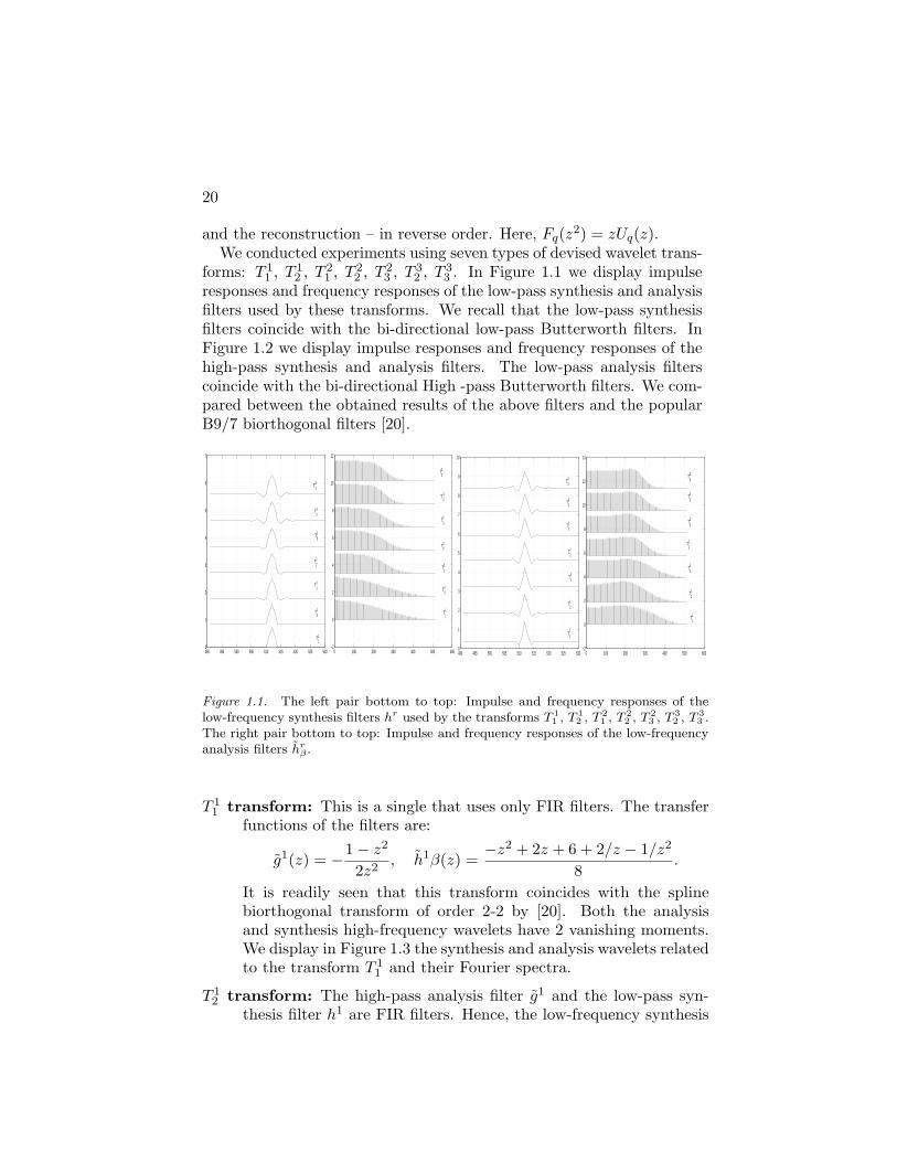
responses and frequency responses of the low-pass synthesis and analysisfilters used by these transforms. We recall that the low-pass synthesisfilters coincide with the bi-directional low-pass Butterworth filters. InFigure 1.2 we display impulse responses and frequency responses of thehigh-pass synthesis and analysis filters. The low-pass analysis filterscoincide with the bi-directional High -pass Butterworth filters. We com-pared between the obtained results of the above filters and the popularB9/7 biorthogonal filters [20].
490 495 500 505 510 515 520 525 5300
1
2
3
4
5
6
7
T11
T12
T21
T22
T23
T32
T33
0 100 200 300 400 500 600−2
0
2
4
6
8
10
12
T33
T 32
T23
T22
T21
T12
T11
490 495 500 505 510 515 520 525 5300
1
2
3
4
5
6
7
8
9
10
T22
T23
T32
T33
T21
T12
T11
0 100 200 300 400 500 600−2
0
2
4
6
8
10
12
14
T22
T23
T32
T33
T21
T12
T11
Figure 1.1. The left pair bottom to top: Impulse and frequency responses of thelow-frequency synthesis filters hr used by the transforms T 1
1 , T 12 , T 2
1 , T 22 , T 2
3 , T 32 , T 3
3 .The right pair bottom to top: Impulse and frequency responses of the low-frequencyanalysis filters hr
β .
T 11 transform: This is a single that uses only FIR filters. The transfer
functions of the filters are:
g1(z) = −1− z2
2z2, h1β(z) =
−z2 + 2z + 6 + 2/z − 1/z2
8.
It is readily seen that this transform coincides with the splinebiorthogonal transform of order 2-2 by [20]. Both the analysisand synthesis high-frequency wavelets have 2 vanishing moments.We display in Figure 1.3 the synthesis and analysis wavelets relatedto the transform T 1
1 and their Fourier spectra.
T 12 transform: The high-pass analysis filter g1 and the low-pass syn-
thesis filter h1 are FIR filters. Hence, the low-frequency synthesis
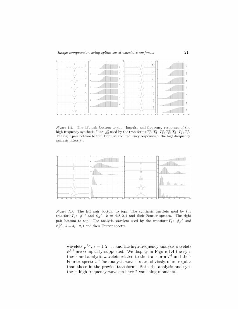
Image compression using spline based wavelet transforms 21
490 495 500 505 510 515 520 525 5300
2
4
6
8
10
12
T22
T21
T12
T11
T23
T32
T33
0 100 200 300 400 500 600−2
0
2
4
6
8
10
12
14
T22
T23
T32
T33
T21
T12
T11
490 495 500 505 510 515 520 525 5300
1
2
3
4
5
6
7
8
9
10
T22
T21
T12
T11
T23
T32
T33
0 100 200 300 400 500 6000
2
4
6
8
10
12
T22
T23
T32
T33
T21
T12
T11
Figure 1.2. The left pair bottom to top: Impulse and frequency responses of thehigh-frequency synthesis filters gr
β used by the transforms T 11 , T 1
2 , T 21 , T 2
2 , T 23 , T 3
2 , T 33 .
The right pair bottom to top: Impulse and frequency responses of the high-frequencyanalysis filters gr.
440 460 480 500 520 540 560 5800
0.5
1
1.5
2
2.5
3
3.5
4
4.5
0 100 200 300 400 500 6000
2
4
6
8
10
12
14
16
440 460 480 500 520 540 560 5800
1
2
3
4
5
6
7
8
0 100 200 300 400 500 6000
2
4
6
8
10
12
14
16
18
20
Figure 1.3. The left pair bottom to top: The synthesis wavelets used by thetransformT 1
2 : ϕ1,4 and ψ1,kβ , k = 4, 3, 2, 1 and their Fourier spectra. The right
pair bottom to top: The analysis wavelets used by the transformT 11 : ϕ1,4
β and
ψ1,kβ , k = 4, 3, 2, 1 and their Fourier spectra.
wavelets ϕ1,s, s = 1, 2, . . . and the high-frequency analysis waveletsψ1,1 are compactly supported. We display in Figure 1.4 the syn-thesis and analysis wavelets related to the transform T 1
1 and theirFourier spectra. The analysis wavelets are obviosly more regularthan those in the previos transform. Both the analysis and syn-thesis high-frequency wavelets have 2 vanishing moments.
22
440 460 480 500 520 540 560 5800
0.5
1
1.5
2
2.5
3
3.5
4
4.5
0 100 200 300 400 500 6000
2
4
6
8
10
12
14
16
18
440 460 480 500 520 540 560 5800
1
2
3
4
5
6
7
0 100 200 300 400 500 600−5
0
5
10
15
20
25
Figure 1.4. The left pair bottom to top: The synthesis wavelets used by thetransformT 1
2 : ϕ1,4 and ψ1,kβ , k = 4, 3, 2, 1 and their Fourier spectra. The right
pair bottom to top: The analysis wavelets used by the transformT 12 : ϕ1,4
β and
ψ1,kβ , k = 4, 3, 2, 1 and their Fourier spectra.
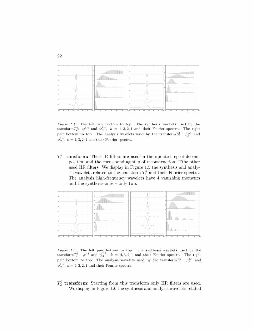
T 21 transform: The FIR filters are used in the update step of decom-
position and the corresponding step of reconstruction. Tthe otherused IIR filters. We display in Figure 1.5 the synthesis and analy-sis wavelets related to the transform T 2
1 and their Fourier spectra.The analysis high-frequency wavelets have 4 vanishing momentsand the synthesis ones – only two.
440 460 480 500 520 540 560 5800
0.5
1
1.5
2
2.5
3
3.5
4
4.5
0 100 200 300 400 500 600−2
0
2
4
6
8
10
12
14
16
18
440 460 480 500 520 540 560 5800
1
2
3
4
5
6
7
0 100 200 300 400 500 600−2
0
2
4
6
8
10
12
14
16
18
Figure 1.5. The left pair bottom to top: The synthesis wavelets used by thetransformT 2
1 : ϕ2,4 and ψ2,kβ , k = 4, 3, 2, 1 and their Fourier spectra. The right
pair bottom to top: The analysis wavelets used by the transformT 21 : ϕ2,4
β and
ψ2,kβ , k = 4, 3, 2, 1 and their Fourier spectra.
T 22 transform: Starting from this transform only IIR filters are used.
We display in Figure 1.6 the synthesis and analysis wavelets related
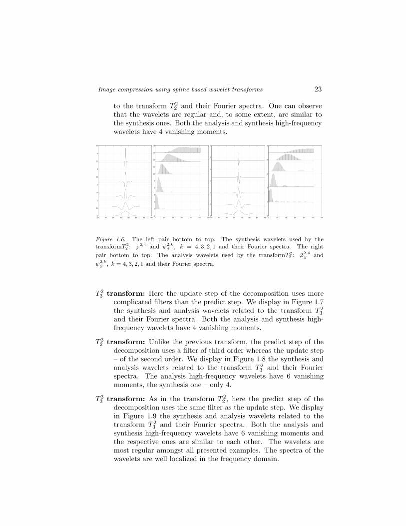
Image compression using spline based wavelet transforms 23
to the transform T 22 and their Fourier spectra. One can observe
that the wavelets are regular and, to some extent, are similar tothe synthesis ones. Both the analysis and synthesis high-frequencywavelets have 4 vanishing moments.
440 460 480 500 520 540 560 5800
0.5
1
1.5
2
2.5
3
3.5
4
4.5
0 100 200 300 400 500 600−2
0
2
4
6
8
10
12
14
16
18
440 460 480 500 520 540 560 5800
1
2
3
4
5
6
0 100 200 300 400 500 600−5
0
5
10
15
20
Figure 1.6. The left pair bottom to top: The synthesis wavelets used by thetransformT 2
2 : ϕ2,4 and ψ2,kβ , k = 4, 3, 2, 1 and their Fourier spectra. The right
pair bottom to top: The analysis wavelets used by the transformT 22 : ϕ2,4
β and
ψ2,kβ , k = 4, 3, 2, 1 and their Fourier spectra.
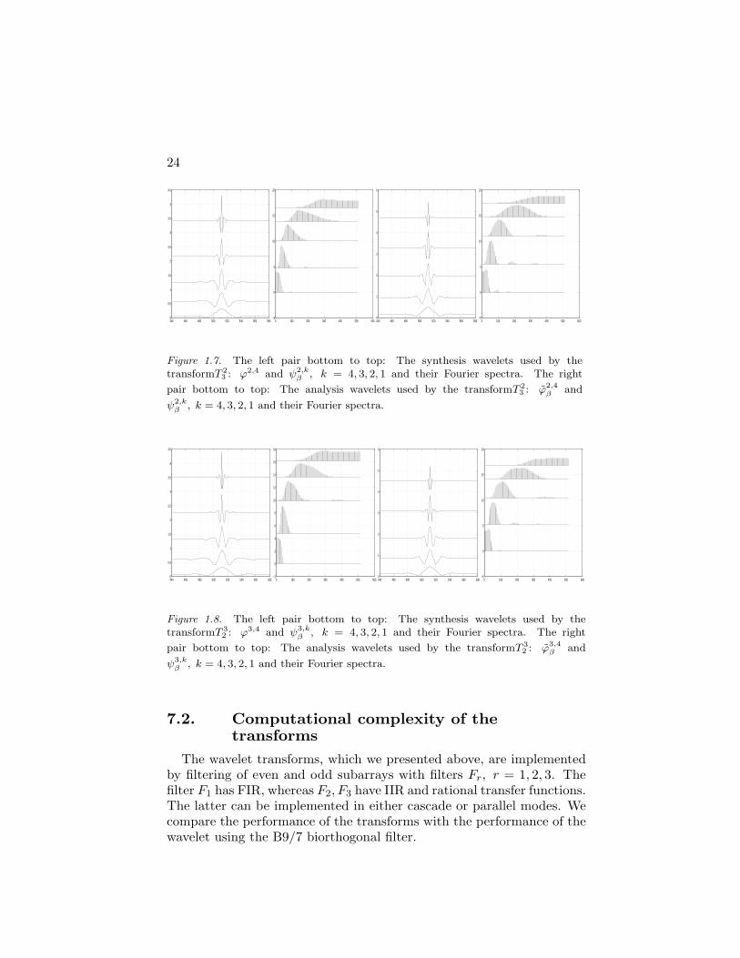
T 23 transform: Here the update step of the decomposition uses more
complicated filters than the predict step. We display in Figure 1.7the synthesis and analysis wavelets related to the transform T 2
3
and their Fourier spectra. Both the analysis and synthesis high-frequency wavelets have 4 vanishing moments.
T 32 transform: Unlike the previous transform, the predict step of the
decomposition uses a filter of third order whereas the update step– of the second order. We display in Figure 1.8 the synthesis andanalysis wavelets related to the transform T 2
3 and their Fourierspectra. The analysis high-frequency wavelets have 6 vanishingmoments, the synthesis one – only 4.
T 33 transform: As in the transform T 2
2 , here the predict step of thedecomposition uses the same filter as the update step. We displayin Figure 1.9 the synthesis and analysis wavelets related to thetransform T 2
3 and their Fourier spectra. Both the analysis andsynthesis high-frequency wavelets have 6 vanishing moments andthe respective ones are similar to each other. The wavelets aremost regular amongst all presented examples. The spectra of thewavelets are well localized in the frequency domain.
24
440 460 480 500 520 540 560 5800
0.5
1
1.5
2
2.5
3
3.5
4
4.5
0 100 200 300 400 500 600−5
0
5
10
15
20
440 460 480 500 520 540 560 5800
1
2
3
4
5
6
0 100 200 300 400 500 600−5
0
5
10
15
20
Figure 1.7. The left pair bottom to top: The synthesis wavelets used by thetransformT 2
3 : ϕ2,4 and ψ2,kβ , k = 4, 3, 2, 1 and their Fourier spectra. The right
pair bottom to top: The analysis wavelets used by the transformT 23 : ϕ2,4
β and
ψ2,kβ , k = 4, 3, 2, 1 and their Fourier spectra.
440 460 480 500 520 540 560 5800
0.5
1
1.5
2
2.5
3
3.5
4
4.5
0 100 200 300 400 500 600−2
0
2
4
6
8
10
12
14
16
18
440 460 480 500 520 540 560 5800
1
2
3
4
5
6
0 100 200 300 400 500 600−5
0
5
10
15
20
Figure 1.8. The left pair bottom to top: The synthesis wavelets used by thetransformT 3
2 : ϕ3,4 and ψ3,kβ , k = 4, 3, 2, 1 and their Fourier spectra. The right
pair bottom to top: The analysis wavelets used by the transformT 32 : ϕ3,4
β and
ψ3,kβ , k = 4, 3, 2, 1 and their Fourier spectra.
7.2. Computational complexity of thetransforms
The wavelet transforms, which we presented above, are implementedby filtering of even and odd subarrays with filters Fr, r = 1, 2, 3. Thefilter F1 has FIR, whereas F2, F3 have IIR and rational transfer functions.The latter can be implemented in either cascade or parallel modes. Wecompare the performance of the transforms with the performance of thewavelet using the B9/7 biorthogonal filter.
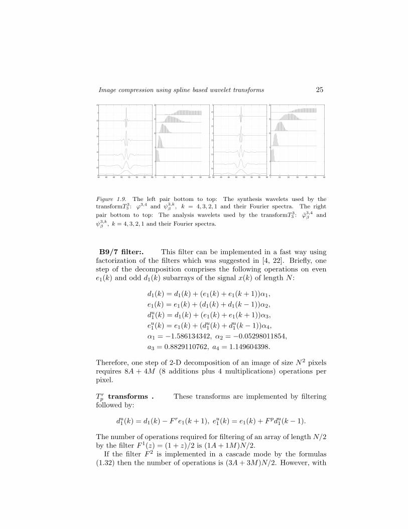
Image compression using spline based wavelet transforms 25
440 460 480 500 520 540 560 5800
0.5
1
1.5
2
2.5
3
3.5
4
4.5
0 100 200 300 400 500 600−5
0
5
10
15
20
440 460 480 500 520 540 560 5800
0.5
1
1.5
2
2.5
3
3.5
4
4.5
5
0 100 200 300 400 500 600−5
0
5
10
15
20
Figure 1.9. The left pair bottom to top: The synthesis wavelets used by thetransformT 3
3 : ϕ3,4 and ψ3,kβ , k = 4, 3, 2, 1 and their Fourier spectra. The right
pair bottom to top: The analysis wavelets used by the transformT 33 : ϕ3,4
β and
ψ3,kβ , k = 4, 3, 2, 1 and their Fourier spectra.
B9/7 filter:. This filter can be implemented in a fast way usingfactorization of the filters which was suggested in [4, 22]. Briefly, onestep of the decomposition comprises the following operations on evene1(k) and odd d1(k) subarrays of the signal x(k) of length N :
d1(k) = d1(k) + (e1(k) + e1(k + 1))α1,
e1(k) = e1(k) + (d1(k) + d1(k − 1))α2,
du1(k) = d1(k) + (e1(k) + e1(k + 1))α3,
eu1(k) = e1(k) + (du
1(k) + du1(k − 1))α4,
α1 = −1.586134342, α2 = −0.05298011854,a3 = 0.8829110762, a4 = 1.149604398.
Therefore, one step of 2-D decomposition of an image of size N2 pixelsrequires 8A + 4M (8 additions plus 4 multiplications) operations perpixel.
T rp transforms . These transforms are implemented by filtering
followed by:
du1(k) = d1(k)− F re1(k + 1), eu
1(k) = e1(k) + F pdu1(k − 1).
The number of operations required for filtering of an array of length N/2by the filter F 1(z) = (1 + z)/2 is (1A + 1M)N/2.
If the filter F 2 is implemented in a cascade mode by the formulas(1.32) then the number of operations is (3A + 3M)N/2. However, with
26
two processors the filtering can be implemented in a parallel which cor-responds to (1.33). Then, each processor performs only (2A + 2M)N/2operations.
Implementation of the filter F 3 in a cascade mode using (1.34) re-quires (5A + 5M)N/2 operations. With three processors the filteringis implemented in a parallel which corresponds to Eq. (1.35). Theneach processor performs only (3A+2M)N/2 operations. Moreover, thisfiltering can be conducted with integers.
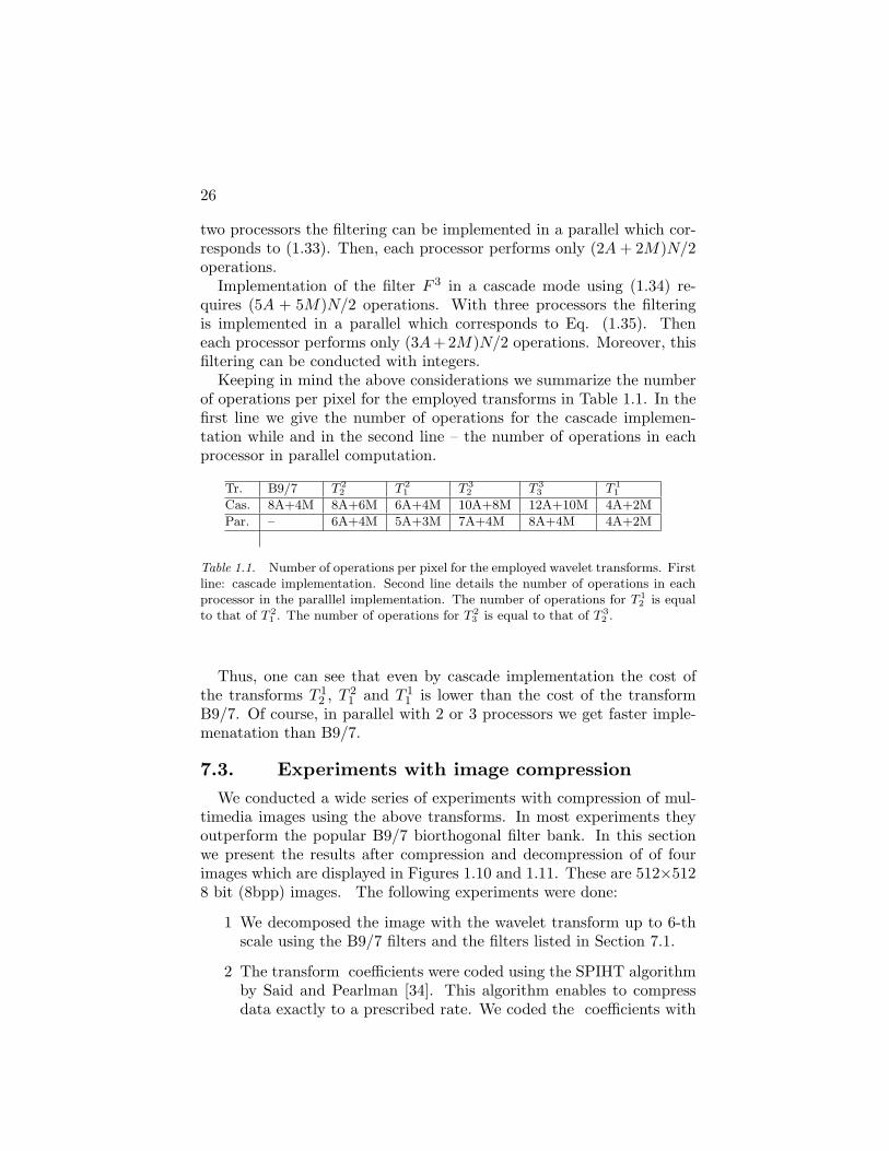
Keeping in mind the above considerations we summarize the numberof operations per pixel for the employed transforms in Table 1.1. In thefirst line we give the number of operations for the cascade implemen-tation while and in the second line – the number of operations in eachprocessor in parallel computation.
Tr. B9/7 T 22 T 2
1 T 32 T 3
3 T 11
Cas. 8A+4M 8A+6M 6A+4M 10A+8M 12A+10M 4A+2M
Par. – 6A+4M 5A+3M 7A+4M 8A+4M 4A+2M
Table 1.1. Number of operations per pixel for the employed wavelet transforms. Firstline: cascade implementation. Second line details the number of operations in eachprocessor in the paralllel implementation. The number of operations for T 1
2 is equalto that of T 2
1 . The number of operations for T 23 is equal to that of T 3
2 .
Thus, one can see that even by cascade implementation the cost ofthe transforms T 1
2 , T 21 and T 1
1 is lower than the cost of the transformB9/7. Of course, in parallel with 2 or 3 processors we get faster imple-menatation than B9/7.
7.3. Experiments with image compressionWe conducted a wide series of experiments with compression of mul-
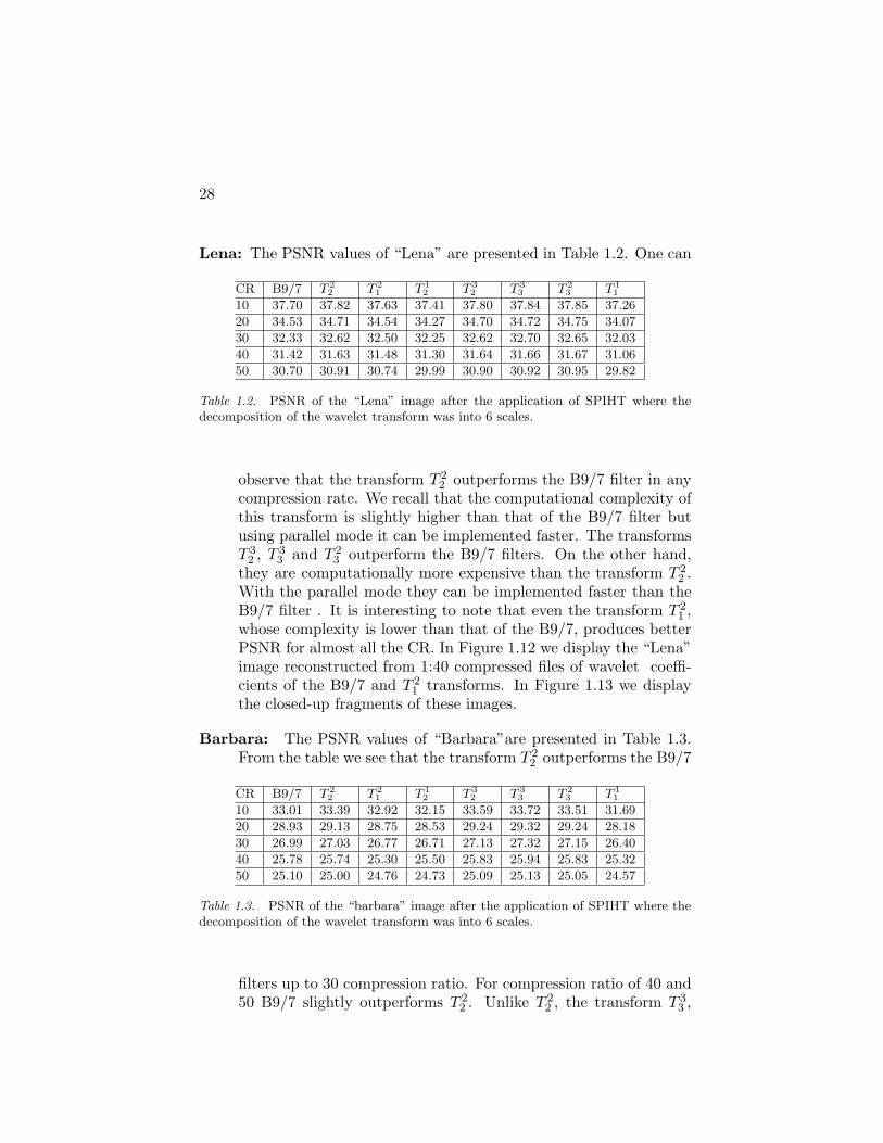
timedia images using the above transforms. In most experiments theyoutperform the popular B9/7 biorthogonal filter bank. In this sectionwe present the results after compression and decompression of of fourimages which are displayed in Figures 1.10 and 1.11. These are 512×5128 bit (8bpp) images. The following experiments were done:
1 We decomposed the image with the wavelet transform up to 6-thscale using the B9/7 filters and the filters listed in Section 7.1.
2 The transform coefficients were coded using the SPIHT algorithmby Said and Pearlman [34]. This algorithm enables to compressdata exactly to a prescribed rate. We coded the coefficients with
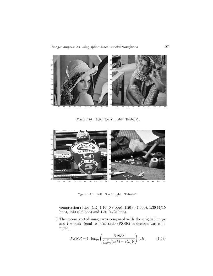
Image compression using spline based wavelet transforms 27
50 100 150 200 250 300 350 400 450 500
50
100
150
200
250
300
350
400
450
500
50 100 150 200 250 300 350 400 450 500
50
100
150
200
250
300
350
400
450
500
Figure 1.10. Left: “Lena”, right: “Barbara”.
50 100 150 200 250 300 350 400 450 500
50
100
150
200
250
300
350
400
450
500
50 100 150 200 250 300 350 400 450 500
50
100
150
200
250
300
350
400
450
500
Figure 1.11. Left: “Car”, right: “Fabrics”.
compression ratios (CR) 1:10 (0.8 bpp), 1:20 (0.4 bpp), 1:30 (4/15bpp), 1:40 (0.2 bpp) and 1:50 (4/25 bpp).
3 The reconstructed image was compared with the original imageand the peak signal to noise ratio (PSNR) in decibels was com-puted.
PSNR = 10 log10
(N 2552
∑Nk=1(x(k)− x(k))2
)dB, (1.43)
28
Lena: The PSNR values of “Lena” are presented in Table 1.2. One can
CR B9/7 T 22 T 2
1 T 12 T 3
2 T 33 T 2
3 T 11
10 37.70 37.82 37.63 37.41 37.80 37.84 37.85 37.26
20 34.53 34.71 34.54 34.27 34.70 34.72 34.75 34.07
30 32.33 32.62 32.50 32.25 32.62 32.70 32.65 32.03
40 31.42 31.63 31.48 31.30 31.64 31.66 31.67 31.06
50 30.70 30.91 30.74 29.99 30.90 30.92 30.95 29.82
Table 1.2. PSNR of the “Lena” image after the application of SPIHT where thedecomposition of the wavelet transform was into 6 scales.
observe that the transform T 22 outperforms the B9/7 filter in any
compression rate. We recall that the computational complexity ofthis transform is slightly higher than that of the B9/7 filter butusing parallel mode it can be implemented faster. The transformsT 3
2 , T 33 and T 2
3 outperform the B9/7 filters. On the other hand,they are computationally more expensive than the transform T 2
2 .With the parallel mode they can be implemented faster than theB9/7 filter . It is interesting to note that even the transform T 2
1 ,whose complexity is lower than that of the B9/7, produces betterPSNR for almost all the CR. In Figure 1.12 we display the “Lena”image reconstructed from 1:40 compressed files of wavelet coeffi-cients of the B9/7 and T 2
1 transforms. In Figure 1.13 we displaythe closed-up fragments of these images.
Barbara: The PSNR values of “Barbara”are presented in Table 1.3.From the table we see that the transform T 2
2 outperforms the B9/7
CR B9/7 T 22 T 2
1 T 12 T 3
2 T 33 T 2
3 T 11
10 33.01 33.39 32.92 32.15 33.59 33.72 33.51 31.69
20 28.93 29.13 28.75 28.53 29.24 29.32 29.24 28.18
30 26.99 27.03 26.77 26.71 27.13 27.32 27.15 26.40
40 25.78 25.74 25.30 25.50 25.83 25.94 25.83 25.32
50 25.10 25.00 24.76 24.73 25.09 25.13 25.05 24.57
Table 1.3. PSNR of the “barbara” image after the application of SPIHT where thedecomposition of the wavelet transform was into 6 scales.
filters up to 30 compression ratio. For compression ratio of 40 and50 B9/7 slightly outperforms T 2
2 . Unlike T 22 , the transform T 3
3 ,
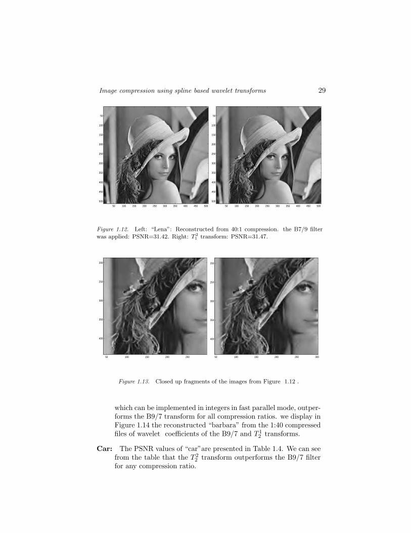
Image compression using spline based wavelet transforms 29
50 100 150 200 250 300 350 400 450 500
50
100
150
200
250
300
350
400
450
500
50 100 150 200 250 300 350 400 450 500
50
100
150
200
250
300
350
400
450
500
Figure 1.12. Left: “Lena”: Reconstructed from 40:1 compression. the B7/9 filterwas applied: PSNR=31.42. Right: T 2
1 transform: PSNR=31.47.
50 100 150 200 250
200
250
300
350
400
50 100 150 200 250 300
200
250
300
350
400
Figure 1.13. Closed up fragments of the images from Figure 1.12 .
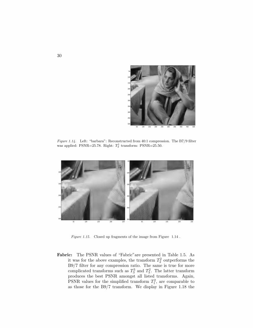
which can be implemented in integers in fast parallel mode, outper-forms the B9/7 transform for all compression ratios. we display inFigure 1.14 the reconstructed “barbara” from the 1:40 compressedfiles of wavelet coefficients of the B9/7 and T 1
2 transforms.
Car: The PSNR values of “car”are presented in Table 1.4. We can seefrom the table that the T 2
2 transform outperforms the B9/7 filterfor any compression ratio.
30
50 100 150 200 250 300 350 400 450 500
50
100
150
200
250
300
350
400
450
500
Figure 1.14. Left: “barbara”: Reconstructed from 40:1 compression. The B7/9 filterwas applied: PSNR=25.78. Right: T 1
2 transform: PSNR=25.50.
50 100 150 200 250
100
150
200
250
300
50 100 150 200 250
50
100
150
200
250
300
Figure 1.15. Closed up fragments of the image from Figure 1.14 .
Fabric: The PSNR values of “Fabric”are presented in Table 1.5. Asit was for the above examples, the transform T 2
2 outperforms theB9/7 filter for any compression ratio. The same is true for morecomplicated transforms such as T 3
3 and T 23 . The latter transform
produces the best PSNR amongst all listed transforms. Again,PSNR values for the simplified transform T 2
1 , are comparable toas those for the B9/7 transform. We display in Figure 1.18 the
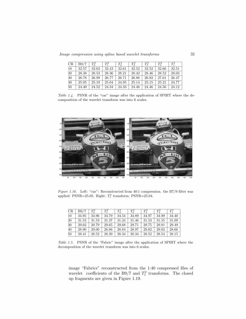
Image compression using spline based wavelet transforms 31
CR B9/7 T 22 T 2
1 T 12 T 3
2 T 33 T 2
3 T 11
10 32.57 32.63 32.43 32.61 32.52 32.52 32.66 32.51
20 28.38 28.53 28.36 28.21 28.42 28.46 28.52 28.03
30 26.78 26.99 26.77 26.71 26.88 26.92 27.01 26.47
40 25.05 25.19 25.04 24.95 25.14 25.15 25.21 24.77
50 24.40 24.52 24.34 24.33 24.46 24.46 24.56 24.12
Table 1.4. PSNR of the “car” image after the application of SPIHT where the de-composition of the wavelet transform was into 6 scales.
50 100 150 200 250 300 350 400 450 500
50
100
150
200
250
300
350
400
450
500
50 100 150 200 250 300 350 400 450 500
50
100
150
200
250
300
350
400
450
500
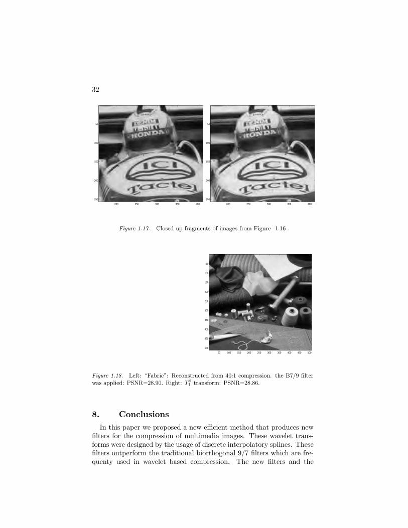
Figure 1.16. Left: “car”: Reconstructed from 40:1 compression. the B7/9 filter wasapplied: PSNR=25.05. Right: T 2
1 transform: PSNR=25.04.
CR B9/7 T 22 T 2
1 T 12 T 3
2 T 33 T 2
3 T 11
10 34.95 34.96 34.79 34.54 34.89 34.97 34.99 34.40
20 31.53 31.53 31.37 31.24 31.46 31.53 31.55 31.09
30 29.62 29.79 29.65 29.68 29.71 29.75 29.81 29.49
40 28.90 29.00 28.86 28.84 28.97 29.02 29.02 28.66
50 28.41 28.52 28.39 28.34 28.34 28.52 28.54 28.15
Table 1.5. PSNR of the “Fabric” image after the application of SPIHT where thedecomposition of the wavelet transform was into 6 scales.
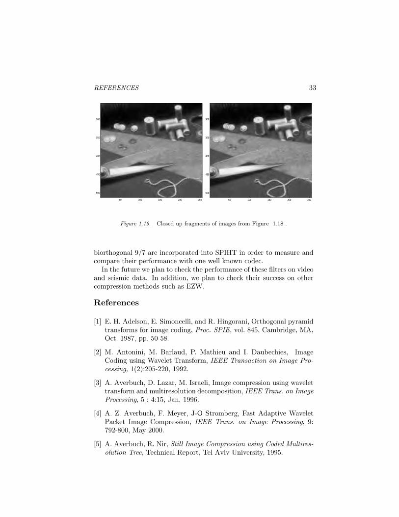
image “Fabrics” reconstructed from the 1:40 compressed files ofwavelet coefficients of the B9/7 and T 2
1 transforms. The closedup fragments are given in Figure 1.19.
32
200 250 300 350 400
50
100
150
200
250
200 250 300 350 400
50
100
150
200
250
Figure 1.17. Closed up fragments of images from Figure 1.16 .
50 100 150 200 250 300 350 400 450 500
50
100
150
200
250
300
350
400
450
500
Figure 1.18. Left: “Fabric”: Reconstructed from 40:1 compression. the B7/9 filterwas applied: PSNR=28.90. Right: T 2
1 transform: PSNR=28.86.
8. ConclusionsIn this paper we proposed a new efficient method that produces new
filters for the compression of multimedia images. These wavelet trans-forms were designed by the usage of discrete interpolatory splines. Thesefilters outperform the traditional biorthogonal 9/7 filters which are fre-quenty used in wavelet based compression. The new filters and the
REFERENCES 33
50 100 150 200 250
300
350
400
450
500
50 100 150 200 250
300
350
400
450
500
Figure 1.19. Closed up fragments of images from Figure 1.18 .
biorthogonal 9/7 are incorporated into SPIHT in order to measure andcompare their performance with one well known codec.
In the future we plan to check the performance of these filters on videoand seismic data. In addition, we plan to check their success on othercompression methods such as EZW.
References
[1] E. H. Adelson, E. Simoncelli, and R. Hingorani, Orthogonal pyramidtransforms for image coding, Proc. SPIE, vol. 845, Cambridge, MA,Oct. 1987, pp. 50-58.
[2] M. Antonini, M. Barlaud, P. Mathieu and I. Daubechies, ImageCoding using Wavelet Transform, IEEE Transaction on Image Pro-cessing, 1(2):205-220, 1992.
[3] A. Averbuch, D. Lazar, M. Israeli, Image compression using wavelettransform and multiresolution decomposition, IEEE Trans. on ImageProcessing, 5 : 4:15, Jan. 1996.
[4] A. Z. Averbuch, F. Meyer, J-O Stromberg, Fast Adaptive WaveletPacket Image Compression, IEEE Trans. on Image Processing, 9:792-800, May 2000.
[5] A. Averbuch, R. Nir, Still Image Compression using Coded Multires-olution Tree, Technical Report, Tel Aviv University, 1995.
34
[6] A. Averbuch, M. Israeli, F. Meyer, Speed vs. Quality in Low Bit-RateStill Image Compression, it Signal Processing: Image Communica-tion, 15:231-254, 1999.
[7] A. Averbuch, A. Pevnyi, V. Zheludev A lifting scheme of biorthogo-nal wavelet transform based on discrete interpolatory splines, Proc.SPIE Wavelet Applications in Signal and Image Processing VIII, (A.Aldroubi, A. F. Laine; M. A. Unser; Eds.) 4119:564–575, 2000.
[8] A. Z. Averbuch, A. B. Pevnyi and V. A. Zheludev But-terworth wavelets derived from discrete interpolatory splines:Recursive implementation, to appear in Signal Processing.,www.math.tau.ac.il/∼amir (∼zhel).
[9] A. Averbuch, V. Zheludev Construction of biorthogonal discretewavelet transforms using interpolatory splines, to appear in Appliedand Comp. Harmonic Analysis, www.math.tau.ac.il/∼amir (∼zhel).
[10] A. Averbuch, R. Coifman, F. Meyer, Multi-layered Image Transcrip-tion: Application to a Universal Lossless, submitted.
[11] G. Battle, A block spin construction of ondelettes. Part I. Lemariefunctions, Comm. Math. Phys. 110:601–615, 1987.
[12] Bing-Bing Chai, Jozsef Vass, and Xinhua Zhuang, Significance-Linked Connected Component Analysis for Wavelet Image Coding,IEEE Transaction on Image Processing 8:774-784, June 1999.
[13] M. Boliek, M. J. Gormish , E. L. Schwartz and A. Keith, NextGeneration Image Compression and Manipulation Using CREW,Proc. IEEE ICIP , 1997, http://www.crc.ricoh.com/CREWhttp://www.crc.ricoh.com/ gormish/pdfhttp://www.crc.ricoh.com/CREW/CREW.summary.html
[14] R. Buccigrossi and E. P. Simoncelli, EPWIC: Embedded Predic-tive Wavelet Image Coder, GRASP Laboratory, TR number 414,http://www.cis.upenn.edu/butch/EPWIC/index.html.
[15] Calderbank, R. C., Daubechies, I., Sweldens, W., and Yeo, B. L.Wavelet Transforms that Map Integers to Integers, Applied and Com-putational Harmonic Analysis (ACHA), vol. 5, no. 3, pp. 332-369,1998, http://cm.bell-labs.com/who/wim/papers/integer.pdf.
[16] C. Chrysafis and A. Ortega, Efficient context-based entropy codingfor lossy wavelet image compression, DCC, Data Compression Con-ference, Snowbird, UT, March 25 - 27, 1997. (.ps version availablefrom http://biron.usc.edu/ chrysafi/Publications.html)
[17] C. K. Chui and J. Z. Wang, On compactly supported spline waveletsand a duality principle, Trans. Amer. Math. Soc. 330:903-915, 1992.
REFERENCES 35
[18] R. L. Claypoole Jr., J. M. Davis, W. Sweldens, R. Baraniuk, Non-linear wavelet transforms for image coding via lifting, submitted toIEEE Trans. Image Proc..
[19] Coifman, R. R. and Wickerhauser, M. V., Entropy Based Algo-rithms for Best Basis Selection, IEEE Trans. Information Theory,38:713-718, Mar. 1992.
[20] A. Cohen, I. Daubechies and J.-C. Feauveau, Biorthogonal bases ofcompactly supported wavelets, Commun. on Pure and Appl. Math.’45:485-560, 1992.
[21] I. Daubechies, Ten lectures on wavelets, SIAM. Philadelphia, PA,1992.
[22] I. Daubechies, W. Sweldens, Factoring wavelet transforms into lift-ing steps, J. Fourier Anal. Appl. 4: 247–269, 1998.
[23] D. L. Donoho, Interpolating wavelet transform, Preprint 408, De-partment of Statistics, Stanford University, 1992.
[24] J. Froment and S. Mallat, Second generation compact image codingwith wavelets. in: Wavelets: A Tutorial in Theory and Applications,C.K. Chui, editor, vol. 2, Academic Press, NY, 1992.
[25] C. Herley and M. Vetterli, Wavelets and recursive filter banks,IEEE Trans. Signal Proc.,’ 41(12):2536-2556 1993.
[26] R. Joshi, H. Jafarkhani, J. Kasner, T. Fischer, N. Farvardin, M.Marcellin and R. Bamberger, Comparison of Different Methods ofClassification in Subband Coding of Images, IEEE Trans. ImageProc., 6:1473-1487, November 1997.
[27] P. G. Lemarie, Ondelettes a localisation exponentielle, J. de Math.Pures et Appl. 67:227-236, 1988.
[28] S. M. LoPresto, K. Ramchandran, and M.T. Orchard, Image cod-ing based on mixture modeling of wavelet coefficients and a fastestimation-quantization framework, it IEEE Data Compression Con-ference ’97 Proceedings, pp. 221-230, March 1997.
[29] D. Marpe and H.L. Cycon, Efficient Pre-Coding Tech-niques for Wavelet-Based Image Compression, submitted to PCS,Berlin, 1997. For more information, please see http://www.fhtw-berlin.de/Projekte/Wavelet/
[30] D. Marpe, G. Heising, A. P. Petukhov, and H. L. Cycon, Videocoding using a bilinear image warping motion model and wavelet-based residual coding, Proc. SPIE Conf. on Wavelet Applications inSignal and Image Processing, 3813: 401 – 408, 1999.
[31] A. V. Oppenheim, R. W. Shafer, Discrete-time signal processing,Englewood Cliffs, New York, Prentice Hall, 1989.
36
[32] A. P. Petukhov, Biorthogonal wavelet bases with rational masks andtheir applications, Proc. of St. Petersburg Math. Soc., Vol. 7:168 –193, 1999 (Russian).
[33] A. B. Pevnyi and V. A. Zheludev, On the interpolation by discretesplines with equidistant nodes, J. Appr. Th., 102:286-301, 2000.
[34] A. Said and W. W. Pearlman, A new, fast and efficient image codecbased on set partitioning in hierarchical trees, IEEE Trans. on Circ.and Syst. for Video Tech., 6: 243-250, June 1996.
[35] S. Servetto, K. Ramchandran, M. Orchard, Image Coding Based ona Morphological Representation of Wavelet Data, IEEE Transactionson Image Processing, 8:1161 -1174 Sept. 1999.
[36] J. Shapiro, Embedded image coding using zerotrees of wavelet coef-ficients, IEEE Tran. on Signal Processing, 41: 3445-3462, December1993.
[37] W. Sweldends The lifting scheme: A custom design constructionof biorthogonal wavelets, Appl. Comput. Harm. Anal. 3(2):186-200,1996.
[38] Taubman, D. High Performance Scalable Image Compression withEBCOT, IEEE Tran. on Image Processing, 9:1158 -1170, July 2000.
[39] Tsai, M. J., Villasenor, J. D., and Chen, F. Stack-Run Image Cod-ing, IEEE Trans. CSVT, 6(5):519-521, Oct. 1996.
[40] M. Unser, A. Aldroubi and M. Eden, A family of polynomial splinewavelet transforms, Signal Processing, 30:141-162, 1993.
[41] Saha, S. and Vemuri, R. Adaptive Wavelet Coding of MultimediaImages, Proc. ACM Multimedia Conference, Nov. 1999.
[42] G. Strang, and T. Nguen, Wavelets and filter banks, Wellesley-Cambridge Press, 1996.
[43] V. A. Zheludev, Periodic splines and the fast Fourier transform,Comput. Math. Math. Phys., 32(2):149-165, 1992.
[44] Xiong, Z., Ramachandran, K. and Orchard, M. T. Space-FrequencyQuantization for Wavelet Image Coding, IEEE Trans. IP, vol. 6, no.5, May 1997, pp. 677-693,
[45] V. A. Zheludev, Wavelet analysis in spaces of slowly growing splinesvia integral representation, Real Analysis Exchange, 24:229-261,1998/99.
[46] W/IEC JTC1/SC29/WG1 N505, Call for contributions forJPEG2000 (ITC 1.29.14, 15444): Image coding system, 1997.
[47] International Organisation for Standardisation (ISO). Call for con-tributions for JPEG 2000 (JTC 1.29.14, 15444): Image Coding Sys-tem, March 1997. ISO/IEC JTCI/SC29/WG1 N505.