NBER WORKING PAPER SERIES

IMPERFECT SUBSTITUTION BETWEEN IMMIGRANTS AND NATIVES:A REAPPRAISAL

George J. BorjasJeffrey Grogger

Gordon H. Hanson

Working Paper 13887http://www.nber.org/papers/w13887

NATIONAL BUREAU OF ECONOMIC RESEARCH1050 Massachusetts Avenue

Cambridge, MA 02138March 2008

We are grateful to Giovanni Peri for providing us with the underlying programs and data used in theOttaviano and Peri (2007) study, and to Alberto Abadie for clarifying an issue regarding alternativeweighting schemes in STATA. All of the programs and data that underlie our analysis are availableon request from the authors. The views expressed herein are those of the author(s) and do not necessarilyreflect the views of the National Bureau of Economic Research.

NBER working papers are circulated for discussion and comment purposes. They have not been peer-reviewed or been subject to the review by the NBER Board of Directors that accompanies officialNBER publications.

© 2008 by George J. Borjas, Jeffrey Grogger, and Gordon H. Hanson. All rights reserved. Short sectionsof text, not to exceed two paragraphs, may be quoted without explicit permission provided that fullcredit, including © notice, is given to the source.

Imperfect Substitution between Immigrants and Natives: A ReappraisalGeorge J. Borjas, Jeffrey Grogger, and Gordon H. HansonNBER Working Paper No. 13887March 2008JEL No. J01,J61

ABSTRACT

In a recent paper, Ottaviano and Peri (2007a) report evidence that immigrant and native workers arenot perfect substitutes within narrowly defined skill groups. The resulting complementarities haveimportant policy implications because immigration may then raise the wage of many native-born workers.We examine the Ottaviano-Peri empirical exercise and show that their finding of imperfect substitutionis fragile and depends on the way the sample of working persons is constructed. There is a great dealof heterogeneity in labor market attachment among workers and the finding of imperfect substitutiondisappears once the analysis adjusts for such heterogeneity. As an example, the finding of immigrant-nativecomplementarity evaporates simply by removing high school students from the data (under the Ottavianoand Peri classification, currently enrolled high school juniors and seniors are included among highschool dropouts, which substantially increases the counts of young low-skilled workers ). More generally,we cannot reject the hypothesis that comparably skilled immigrant and native workers are perfect substitutesonce the empirical exercise uses standard methods to carefully construct the variables representingfactor prices and factor supplies.

George J. BorjasKennedy School of GovernmentHarvard University79 JFK StreetCambridge, MA 02138and NBERgborjas@harvard.edu

Jeffrey GroggerIrving B. Harris Professor of Urban PolicyHarris School of Public PolicyUniversity of Chicago1155 E. 60th StreetChicago, IL 60637and NBERjgrogger@uchicago.edu

Gordon H. HansonIR/PS 0519University of California, San Diego9500 Gilman DriveLa Jolla, CA 92093-0519and NBERgohanson@ucsd.edu

2

Imperfect Substitution between Immigrants and Natives: A Reappraisal

George J. Borjas, Jeffrey Grogger, and Gordon H. Hanson* I. Introduction

A central issue in the ongoing immigration debate is how immigrants affect the economic

opportunities of American workers. Because immigration increases labor supply, there is a

concern that immigration puts downward pressure on natives' wages. Despite an enormous

volume of research on the subject, however, the literature has yet to reach a consensus.1 In

influential recent work, Card (2001) suggests that the effects of immigrants on wages are small,

whereas Borjas (2003) finds that recent immigration has reduced wages, particularly for low-

skill natives.

If immigration increases labor supply, how could it fail to lower wages? One possibility

is that immigrants and natives are imperfect substitutes in employment. Under imperfect

substitutability, immigrants complement native workers, thereby raising the marginal product of

native labor.

Here again, the literature offers conflicting results. Ottaviano and Peri (2007a; hereafter,

OP) find evidence of imperfect substitutability, estimating a “median” elasticity of substitution

between comparably skilled immigrants and natives of around 6.6.2 Jaeger (1996. revised 2007),

Borjas, Grogger, and Hanson, (2006; hereafter, BGH), and Aydemir and Borjas (2007), in

*We are grateful to Giovanni Peri for providing us with the underlying programs and data used in the

Ottaviano and Peri (2007) study, and to Alberto Abadie for clarifying an issue regarding alternative weighting schemes in STATA. All of the programs and data that underlie our analysis are available on request from the authors.

1 See Borjas (1999) for a review of the literature. 2 For related work, see Ottaviano and Peri (2007b, 2007c).

3

contrast, find evidence of perfect substitutability, which implies that the elasticity of substitution

is infinite.

The elasticity of substitution between comparably skilled immigrants and natives is a

critical parameter for assessing the wage effects of immigration. OP's estimate implies that the

immigrant influx that entered the United States between 1990 and 2004 would have raised native

wages by 1.8 percent in the long run. In contrast, OP also show that if the elasticity of

substitution were infinite, the 1990-2004 immigrant influx would have barely changed the long-

run wage of native workers, but would have reduced the wage of low-skill natives by 4 percent.3

In short, the value of the elasticity of substitution between immigrants and natives is more than

an academic curiosity. The notion that immigration might raise native wages has attracted

considerable attention in the debate over U.S. immigration policy.4 The U.S. Council of

Economic Advisors, in its defense of Bush administration proposals to overhaul how the country

regulates its borders, emphasized findings on the complementarity between immigrants and

natives as evidence that current U.S. immigration benefits native workers.5

In this paper, we reassess the evidence regarding the substitutability of native and

immigrant labor. First, using data from the 1960 to 2000 U.S. censuses and the 2004 American

Community Survey (ACS), we attempt to replicate the OP results. We then show that their

finding of imperfect substitutability is sensitive to the inclusion of workers who have low levels

3 These estimates allow for long-run adjustment in the capital stock in response to immigration. In the

constant returns framework used by OP, it is necessarily the case that immigration does not change the average wage of pre-existing workers in the long run.

4 For coverage of OP’s results in the press and by policy organizations, see Virginia Postrel, “Yes, Immigration May Lift Wages,” The New York Times, November 3, 2005; “Myths and migration, Economics focus,” The Economist, April 8, 2006; Diana Furchtgott-Roth, “Do Immigrants Drive Down Citizens’ Wages? No,” Hudson Institute, April 20, 2006 (http://emp.hudson.org); Daniel Griswold, “Comprehensive Immigration Reform: Finally Getting it Right,” Free Trade Bulletin, No. 29, May 16, 2007, Cato Institute; Fareed Zakaria, “America’s New Know-Nothings,” The Washington Post, May 21, 2007. See also Ottaviano and Peri (2007b, c).

5 The U.S. Council of Economic Advisors concludes, “Our review of economic research finds immigrants not only help fuel the nation's economic growth, but also have an overall positive effect on the income of native-born workers" (“Immigration’s Economic Impact,” CEA White Paper, http://www.whitehouse.gov/cea/pubs.html).

4

of attachment to the workforce. The problem is that the wages of such workers confound demand

and supply factors, whereas the estimating equation used to test for perfect substitution stems

from equations implied by the theory of factor demand, equations that call for data on the rental

price of labor.

We illustrate our critique with a stark example of this problem. We begin by showing that

OP’s finding of imperfect substitutability is sensitive to the inclusion of young students in the

sample. Indeed, merely dropping from the OP sample those 17- and 18-year-olds who were

enrolled in school—the vast majority of whom are high school juniors and seniors—is sufficient

to overturn the OP finding of imperfect substitution between immigrant and native men.

The reason is that OP misclassify such students as high school dropouts. This artificially

inflates the number of native dropouts, which in turn reduces the relative immigration shock

facing such low-skill workers. At the same, it raises the wage of low-skill immigrants in relation

to low-skill natives, since working high school students earn even less than true high school

dropouts. In a regression of relative immigrant wages on the relative immigration shock, this

negatively biases the coefficient on the relative immigration shock. Since the coefficient on the

relative immigration shock is equal to (minus) the inverse elasticity of substitution between

immigrants and natives, the result is a downward-biased estimate of the elasticity of substitution.

Although this simple example is sufficient to illustrate the fragility of the OP result, there

is a conceptually more important issue at the core of our critique. To obtain valid estimates of the

elasticities of substitution underlying a system of factor demand equations, it is crucial to pay

careful attention to how the theoretical variables match with the available data. We show that

evidence in favor of imperfect substitution is strongest for samples where average wages depart

the most from the theoretical ideal of the rental price of labor. For instance, the estimated

5

substitution elasticity is sensitive to whether we use annual earnings or weekly earnings to define

wages, whether we focus on men or include women in the sample, and to the extent to which

part-time workers are represented in the sample. Overall, the evidence of labor-market

complementarities between comparably skilled immigrants and natives is fragile. In general, a

carefully designed empirical exercise that matches the theoretical concepts from factor demand

theory with observable measures of prices and supplies fails to reject the hypothesis that

comparably skilled immigrants and native workers are perfect substitutes.

II. Theory and the Estimating Equation

The starting point of the OP study is the three-level CES framework describing the

relation among various factors of production set out in Borjas (2003).6 In that paper, Borjas

argues that the impact of immigration on the labor market can be measured by examining the

wage evolution of workers in narrowly defined skill groups in the national labor market. Skill

groups are defined in terms of both educational attainment and work experience. After

documenting the existence of a strong negative correlation between wages for a particular group

and immigration-induced supply shocks for that group in the national-level data, Borjas

estimates a structural model that allows for cross-effects among groups. The estimated

elasticities of substitution are then used to simulate how wages for each skill group are affected

by immigration-induced supply shocks in all groups.

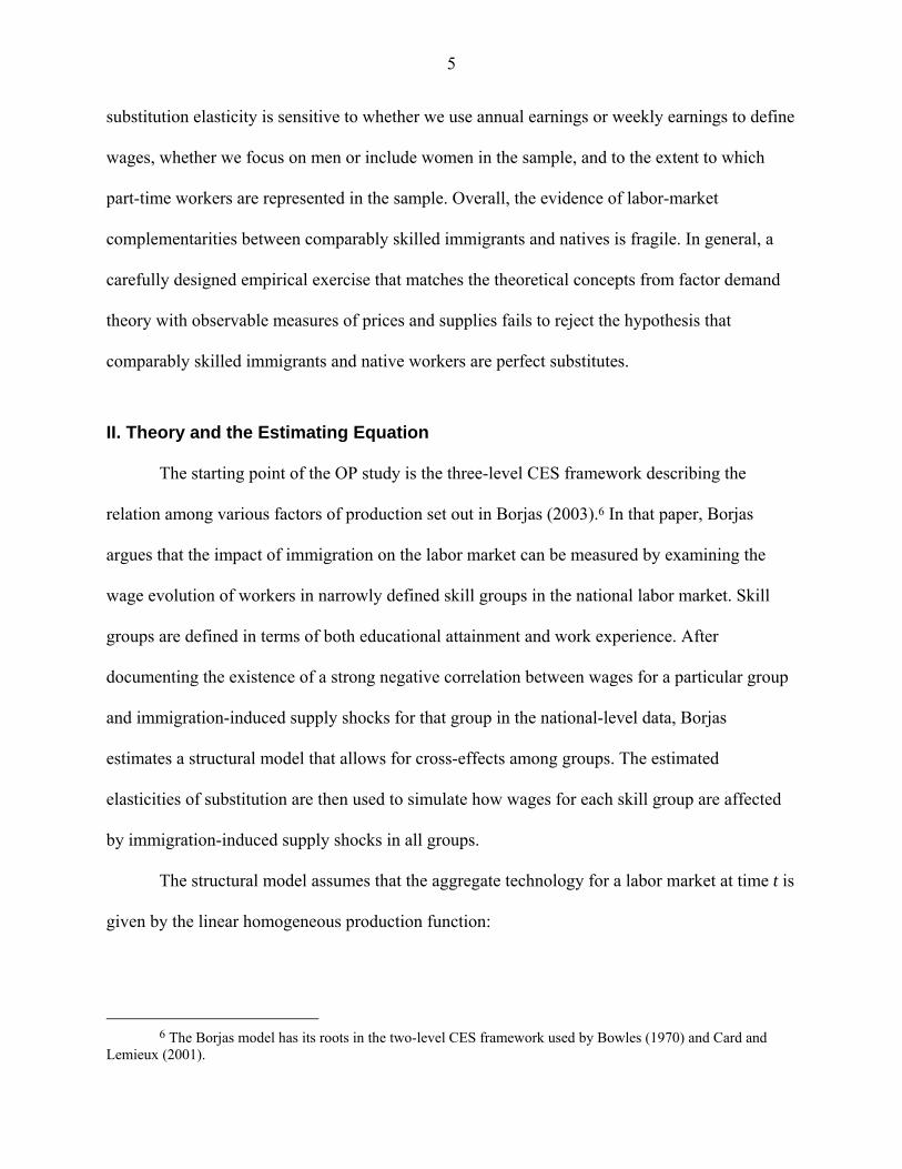
The structural model assumes that the aggregate technology for a labor market at time t is

given by the linear homogeneous production function:

6 The Borjas model has its roots in the two-level CES framework used by Bowles (1970) and Card and

Lemieux (2001).

6

(1) 1/

(1 ) ,vv v

t Lt t Lt tQ K L⎡ ⎤= − λ + λ⎣ ⎦

where Q is output, K is capital, L denotes the aggregate labor input, and v = 1 – 1/σKL, with σKL

being the elasticity of substitution between capital and labor (–∞ < v ≤ 1). For convenience, the

price of the (single) aggregate output is set as the numeraire. Both Borjas (2003) and OP assume

that σKL = 1, so that the aggregate CES production function collapses to a Cobb-Douglas.

The aggregate Lt incorporates the contributions of workers who differ in both educational

attainment and labor market experience. Let:

(2) 1/

t st sts

L Lρ

ρ⎡ ⎤= θ⎢ ⎥⎣ ⎦

∑ ,

where Lst gives the number of workers with education s at time t, and ρ = 1 – 1/σE, with σE being

the elasticity of substitution across these education aggregates (–∞ < ρ ≤ 1). The θst give

technology parameters that shift the relative productivity of education groups, with Σi θst = 1.

Finally, the supply of workers in each education group is itself an aggregation of similarly

educated workers with different years of labor market experience. In particular:

(3) 1/

st sx sxtx

L Lη

η⎡ ⎤= α⎢ ⎥⎣ ⎦∑ ,

where Lsxt gives the number of workers in education group s and experience group x at time t;

and η = 1 – 1/σX, with σX being the elasticity of substitution across experience classes within an

education group (–∞ < η ≤ 1), and Σx αsx = 1. In the Borjas (2003) study, equation (3) imposes

7

the restriction that native (Nsxt) and immigrant (Msxt) workers with the same education and

experience are perfect substitutes in production, and defines Lsxt = Nsxt + Msxt.

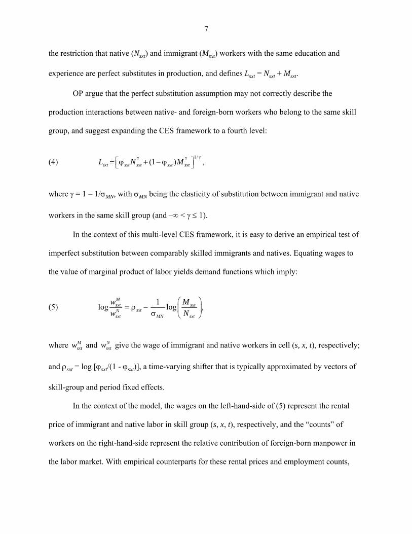
OP argue that the perfect substitution assumption may not correctly describe the

production interactions between native- and foreign-born workers who belong to the same skill

group, and suggest expanding the CES framework to a fourth level:

(4)

1/(1 ) ,sxt sxt sxt sxt sxtL N M

γγ γ⎡ ⎤= ϕ + − ϕ⎣ ⎦

where γ = 1 – 1/σMN, with σMN being the elasticity of substitution between immigrant and native

workers in the same skill group (and –∞ < γ ≤ 1).

In the context of this multi-level CES framework, it is easy to derive an empirical test of

imperfect substitution between comparably skilled immigrants and natives. Equating wages to

the value of marginal product of labor yields demand functions which imply:

(5) 1log log ,Msxt sxt

sxtNsxt MN sxt

w Mw N

⎛ ⎞= ρ − ⎜ ⎟σ ⎝ ⎠

where M

sxtw and Nsxtw give the wage of immigrant and native workers in cell (s, x, t), respectively;

and ρsxt = log [ϕsxt/(1 - ϕsxt)], a time-varying shifter that is typically approximated by vectors of

skill-group and period fixed effects.

In the context of the model, the wages on the left-hand-side of (5) represent the rental

price of immigrant and native labor in skill group (s, x, t), respectively, and the “counts” of

workers on the right-hand-side represent the relative contribution of foreign-born manpower in

the labor market. With empirical counterparts for these rental prices and employment counts,

8

equation (5) can then be used to estimate the parameter σMN and test for perfect substitution

between immigrants and natives. In what follows, we will consider alternative definitions of the

critical price and quantity measures needed to test for perfect substitution and document the

fragility of the OP finding of immigrant-native complementarity.

III. Data

OP and BGH use similar data and analyze it similarly. For example, BGH pool data

aggregated from microdata samples of the 1960-2000 decennial U.S. Censuses; OP add an

additional cross-section drawn from the 2004 American Community Survey (ACS). As has

become standard in this literature, both OP and BGH aggregate individual workers into skill

groups defined by education and experience. Workers are classified into one of four education

groups: high school dropouts, high school graduates, workers with some college, and college

graduates. Workers in each of these education groups are then classified into groups that differ

by their amount of labor market experience. Experience is defined by “labor market exposure,”

or the number of years elapsed since the worker entered the labor market (i.e., current age minus

age at time of labor market entry). Workers who are high school dropouts are assumed to enter

the labor market at age 17; workers who are high school graduates at age 19; workers who have

some college at age 21; and workers who are college graduates at age 23. Workers in each

education group are then classified into one of eight groups depending on the labor market

experience (OP classify these bands as 0 to 4 years or experience, 5 to 9 years of experience, and

so on). These definitions of the education and experience categories define a total of 32 skill

groups at a point in time. OP and BGH then calculate mean wages and the number of working

natives and immigrants for each of the 32 skill groups in each of the available cross-sections.

9

In order to be included in these calculations, OP impose four key restrictions on the

individual-level Census observations. Their sample inclusion criteria restrict the calculation of

mean wages and the counts of working natives and immigrants to persons who:

1. are not residing in group quarters;

2. are aged 17-65, inclusive;

3. worked at least one week in the calendar year prior to the Census, had positive hours

worked per week, and reported positive wage and salary earnings;7

4. have between 0 and 40 years of work experience, inclusive.

After accounting for sampling weights, the mean wage of immigrants and natives in a particular

cell is defined by the simple average of the earnings of immigrant or native workers in the group,

while the number of working immigrants and natives is given by the simple sum of the number

of such workers in the cell. We provide a detailed description of the selection rules used by OP

in the Data Appendix.

Giovanni Peri provided us with the aggregate (cell-level) data used in OP and with the

programs used to construct those data from the Census/ACS microdata. We were able to exactly

replicate the OP mean wages and counts of workers for the 1960, 1970, and 2004 cross-sections.

Despite having access to the underlying programs, we were unable to exactly replicate the OP

cell-level data for the 1980, 1990, and 2000 cross-sections.8 However, the differences between

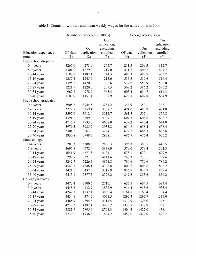
the OP data and the data in our attempted replication are small. Table 1 reports the number of

native workers as well as the mean weekly wage of native workers for each of the 32 skill groups

in the 2000 Census cross-section. Columns (1) and (4) of the table report the statistics in the

7 One relatively minor problem with this restriction is that in some surveys OP use usual hours of work in

the previous calendar year, while in other surveys they use hours worked during the reference week. 8 Giovanni Peri informs us that OP used 1% samples for 1980, 1990, and 2000, even though their text

indicated that they had used the 5% samples. We suspect that this explains our inability to replicate their results exactly.

10

original OP data. Columns (2) and (5) report the respective statistics from our attempted

replication. The counts of native workers in the OP analysis and in our replication differ by an

average of 0.05 percent and the average weekly wage differs by an average of 0.3 percent.

The OP data reported in the first column of Table 1 has one striking feature: there are a

large number of native workers who are classified as high school dropouts with 0-4 years of

experience. In fact, in both the original OP data and in our attempted replication, there are 4.3

million such workers. According to OP, there were more “young” (i.e., workers with 0 to 4 years

of labor market experience) native high school dropouts in the 2000 Census than there were

young high school graduates or young college graduates. Indeed, 25 percent of the native

workers in the youngest experience group appear to be high school dropouts.

These counts of young high school dropouts greatly exceed published totals (2008

Statistical Abstract, Table 265, p. 172). Published sources enumerate all persons (not only

workers) who lack a high school credential and are no longer enrolled in school. Whereas OP

report 4.8 million working high school dropouts (both native- and foreign-born) aged 17-21 in

2000, the Statistical Abstract reports a total of only 2.5 million high school dropouts aged 16-

21.9

How could OP estimate that one-fourth of young native workers are high school dropouts

at a time when dropout rates for young adults averaged only 10.6 percent?10 The answer lies in

the way that they construct their sample. To be counted as a worker in the sample of young high

school dropouts, OP include anyone in the 2000 Census who had not yet received a high school

credential, was between 17 and 21 years old, worked at least one week in 1999, had positive

usual hours of work, and reported positive wage-and-salary earnings for the 1999 calendar year.

9 The OP enumeration of workers for the cell of high school dropouts with 0-4 years of experience is 4.27 million natives and 0.57 million immigrants.

10 This figure is for natives aged 19-28 in 2000 (calculated from the 5 percent 2000 IPUMS sample).

11

This includes many teenagers who work part time. Of course, most of the people who were 17

and 18 years old when the Census enumeration took place on April 1, 2000 were students, and

the vast majority of them were high school students (either juniors or seniors). Many high school

students work, but both their hours of work and their earnings tend to be low.

Compounding the problem, the OP definition of education groups classifies these high

school students as high school dropouts. The reason is that the Census measures completed

schooling. A teenager who is attending 12th grade in April 2000 has only completed 11th grade.

Thus, he will be classified as a high school dropout, even though he is slated to graduate from

high school in the following month or two. Similarly, every 17-year-old high school junior who

works part-time for a few hours a week is classified as a high school dropout in the OP analysis.

As a result, the least-skilled group in the analysis (i.e., workers who are labeled as high

school dropouts and have 0 to 4 years of experience) contains a large number of workers with

low levels of labor market attachment who have little in common with “high school dropouts” as

that term is typically used. Column (3) of Table 1 shows what happens to the enumerated

number of workers when we exclude students (i.e., persons currently enrolled) from the

calculation. The number of native workers in the least-skilled group falls from 4.3 million to less

than 1.3 million. Counts for some of the other skill groups fall significantly as well—mainly in

the skill group of workers with some college and less than 4 years of experience. Note, however,

that the exclusion of students clearly affects the counts in the least-skilled cell the most, because

almost all 17- and 18-year-olds are attending high school.

Table 1 shows another implication of treating high school students as if they were high

school dropouts. Column (4) reports the mean weekly wage of native workers in the OP data;

column (5) reports the slightly different wage data from our replication; and column (6) reports

12

the mean weekly wage if we exclude persons who are enrolled in school. The data show that the

earnings of true high school dropouts—workers who have fewer than 12 years of schooling and

are not enrolled in school—are higher than those of young workers who are still enrolled in high

school. When we exclude the enrolled, the average weekly earnings of the young high school

dropouts rise from around $210 to $310.

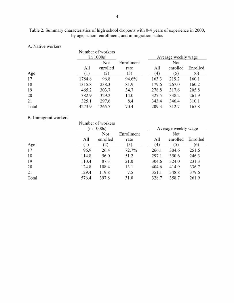
Table 2 shows how the problems introduced by including high school students

differentially affect the samples of immigrant and native workers. Column (1) displays (by age)

the number of workers classified as high school dropouts with 0-4 years of experience, while

column (2) displays the number not enrolled. The exclusion of the enrolled from the OP sample

of high school dropouts aged 17-21 cuts the number of native workers in this low-skill group by

more than two-thirds, while raising their average weekly earnings by nearly 50 percent. In

contrast, the exclusion of the enrolled reduces the number of foreign-born high school dropouts

only by about a third, from 576 thousand to 398 thousand, and raises the average weekly wage

by only about 10 percent, from $329 to $359. In short, the inclusion of the enrolled skews the

data differentially for native and foreign-born workers. We show in the next section that this is

directly responsible for OP's conclusion that immigrant and native men are imperfect substitutes.

Although we have focused on the high school dropout issue to illustrate our point, the

discussion highlights a general problem. The average wage of a skill group in the OP data is

contaminated by the heterogeneity in work attachment among the persons who form that skill

group. As a result, the data on the average wage of a skill group may bear only a weak relation to

the rental price for their labor. Similarly, the number of workers in the skill group does not

reflect the “true” supply of that group. In other words, it does not seem sensible to count a high

school junior as much as a 20-year-old high school dropout (as that term is usually used), and

13

neither does it seem sensible to infer that the average wage of a high school junior is somehow

representative of what the typical high school dropout can command in the labor market.

IV. The Fragility of Immigrant-Native Complementarity

As we have emphasized, the estimation of equation (5) requires that careful attention be

paid to the empirical construction of the two key variables in the analysis—relative wages and

relative supplies. We now document the fragility of the OP finding of imperfect substitution to

this issue.

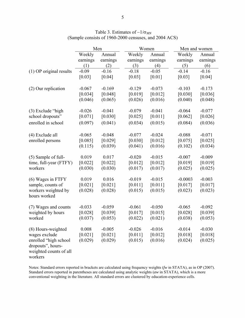
Table 3 reports weighted least squares estimates of the parameter −1/σMN from equation

(5). Each entry in the table comes from a separate regression estimated using the 192

observations that result from stacking the cell-level data for each of the 32 skill groups across the

six Census/ACS cross-sections from 1960 to 2004. In each regression, the dependent variable is

the log of the ratio of mean immigrant wages to mean native wages.11 Following OP, we use two

alternative measures of earnings to calculate the dependent variable: weekly earnings and annual

earnings. In each regression, the key explanatory variable is the log of the ratio of the number of

immigrants to the number of natives. All regressions also include fixed effects for education

groups, experience groups, time periods, education interacted with time periods, experience

interacted with time periods, and education interacted with experience.

Columns (1) and (2) of the table calculate wages and employment counts using the

sample of working men; columns (3) and (4) do the same calculations using the sample of

working women; and columns (5) and (6) do the calculations using the pooled sample of

working men and women. Following OP, all observations in the regression analysis are weighted

11 Following OP, we estimate the regression using the log of the ratio of mean earnings rather than the

more natural difference in the mean of log earnings. The use of the latter variable typically weakens OP’s results.

14

by total employment in the skill group (which is defined by the sum of the number of immigrants

and natives in the cell). Finally, standard errors are clustered by education and experience.

The first row reports estimates from Table 3 of OP, where we have reversed their

reported sign for consistency with our convention of reporting the actual regression coefficient

(i.e., the estimate of −1/σMN). The estimated coefficients for men imply an elasticity of

substitution of 11 (= 1/0.09) when wages are measured by weekly earnings and 6.3 (=1/0.16)

when wages are measured by annual earnings. The second row of Table 4 reports our attempt to

replicate OP’s results. Because we were unable to duplicate their data exactly in three of the

cross-sections, we were also unable to fully replicate their estimates. Nevertheless, our estimated

regression coefficients have similar magnitudes to those reported in the OP paper. Our estimate

of the elasticity of substitution based on annual earnings and the pooled sample of mean and

women is close to the OP “median” estimate of 6.6, which they use to produce their widely cited

simulation results regarding the beneficial effect of immigration on native wages.12 OP designate

the results from the regressions based on annual earnings and the pooled samples as their

preferred specification.

There are two issues related to the OP preferred specification that are worth noting before

we proceed further. First, there is a theoretical difficulty with OP’s preference for using annual

earnings as the wage measure on the left-hand-side of equation (5). As emphasized above, the

relative demand function implied by the CES functional form results from equating the value of

marginal product to the rental price of the worker’s human capital. The ideal wage measure for

this test thus would be one that best represents this rental price. For instance, one might turn to

12 More precisely, in the male-only (female-only) regressions, both the dependent variable and the log of

relative supplies in each cell are calculated using only the sample of working men (women); in the “male and female” regressions, both the dependent variable and the log of relative supplies are calculated using both male and female workers.

15

an hourly measure of the wage, but OP do not analyze hourly wage data. Short of hourly wages,

however, annual earnings confound supply and demand factors to a much greater extent than the

weekly earnings often used to measure wages in the immigration literature. To see this, let yi be

the annual earnings of immigrants in a particular skill cell and yn be the annual earnings of

natives in that cell (for expositional convenience, we omit the subscripts indicating the skill

group and the time period). The ratio of log annual earnings can be written as:

(6) log yi

yn

= log wi

wn

+ log hi

hn

,

where w is the wage rate and h denotes annual hours of work. Substituting from (5), this can be

written as:

(7) 1log log log ,i i

n MN n

y M hy N h

⎛ ⎞= ρ − +⎜ ⎟σ⎝ ⎠

where ρ is a cell-specific constant.

Hours of work for group j depend on a labor supply function that can be written as:

(8) log hj = αj + βj log wj,

where βj is the group-specific labor supply elasticity. The core of the question being analyzed in

this paper presumes that an immigration-induced supply shift influences the wage of the skill

group, so that we can posit the existence of a reduced-form equation that relates the wage of the

group to the size of the immigrant supply shock. In the literature, this type of reduced-form

equation often relates the wage of the group to the immigrant share in the relevant labor market

(where the immigrant share is defined as the fraction of the workforce that is foreign-born). The

16

immigrant share can be approximated by the log ratio of immigrants to natives, log(M/N), so that

the reduced-form relation between the group’s wage and immigration-induced supply shifts can

be written as:

(9) log log ,j jMw dN

= + δ

where δj is the factor price elasticity that relates the wage of natives or immigrants to the

immigrant influx. Combining terms we obtain:

(10) 1log * log .ii i n n

n MN

y My N

⎛ ⎞= ρ + − + β δ − β δ⎜ ⎟σ⎝ ⎠

Equation (10) shows that the regression of the ratio of log annual earnings on log relative

quantities does not identify the parameter of interest, σMN. For instance, the coefficient relating

relative annual earnings to relative quantities could be more negative than that relating relative

wage rates to relative quantities if the native labor supply elasticity is smaller than that of

immigrants. The literature provides no guidance on the size of these labor supply elasticities, but

equation (10) makes clear that annual earnings regressions fail to identify the elasticity of

substitution between immigrants and natives.

A second problem with OP’s reported regression results lies in the calculation of the

standard error. Our replication results in row 2 of Table 4 report two sets of standard errors. In

brackets, we report the standard errors that result when total employment in the cell is treated as

a frequency weight, or “fweight” in STATA. These are the types of standard errors reported in

OP. In parentheses, we report the standard errors that result when the employment counts are

17

treated as so-called analytic weights, or “aweights” in STATA. The use of “fweights” results in

smaller standard errors than the more commonly used "aweights."

Which type of weighting should be preferred? A frequency weight equal to W treats the

corresponding observation as if it represented W identical persons in the population. Frequency

weighting by W is equivalent to duplicating the observation W times and estimating without

weights. Frequency weights are typically used to estimate population marginal distributions

from sample data. In contrast, analytic weights are used to account for differential precision

across observations. Since our observations are based on different numbers of underlying

individual observations, it makes sense to account for differences in precision. However, because

none of the cell-level observations is meant to exactly represent some larger number of persons,

it is difficult to justify using frequency weights.13 As a result of frequency weighting, OP

understate the standard error of their estimated coefficients by about a third.14

The remaining rows of the first two columns of Table 4 present our estimates of the key

regression coefficient from equation (5) as we attempt to deal with the within-cell heterogeneity

noted in the previous section in the sample of working men. We begin with the easiest way of

handling the problem: we simply exclude from the calculation all workers who have not

completed high school, who are enrolled in school, and who are 17 or 18 years old. In other

words, we begin by excluding high school juniors and seniors from the sample of high school

dropouts. Note that this sample restriction only affects the mean wages and employment counts

13 The discussion also raises the question of whether employment in the cell is the correct weighting

variable that should be used, even with analytic weights. The issue of precision suggests that it is the sample size used in calculating the dependent variable—rather than the population estimate of the number of workers in the cell—that should be used as a weight. We will return to this issue below.

14 In fact, there is an exact numerical relationship in the clustered standard errors estimated using the two different types of weights. In personal correspondence, Alberto Abadie has shown that, in the current context, the ratio of the standard error provided by frequency weights to the standard error provided by analytic weights equals the square root of [(J-1)/(J-k)/(N-1)/(N-k)], where J is the number of cells, k is the number of parameters to be estimated, and N is the sum of the frequency weights. In our analysis for men, J = 192, k = 88, and N = 295,622,679 so that the ratio of the two standard errors will be exactly equal to 1.36.

18

in the cell of the youngest high school dropouts in each cross-section. Nevertheless, this change

in the sample definition overturns the conclusion that immigrants and natives are imperfect

substitutes in the sample of working men. As row 3 shows, the regression coefficient based on

male weekly earnings falls to -0.026 with a standard error of 0.097. In other words, the

hypothesis that comparably skilled immigrants and natives are perfect substitutes cannot be

rejected either numerically or statistically.

It is easy to see why the misclassification of high school students as high school dropouts

is such a crucial determinant of OP’s findings. Consider the descriptive statistics summarized in

Tables 1 and 2. The inclusion of high school students in the construction of the sample of

working persons simultaneously increases the number of natives in the cell of native young high

school dropouts and decreases the earnings of that group. Consider now the functional form of

the regression model in equation (5). The inclusion of the high school students effectively creates

a number of cells with a very high count of native workers (hence lowering the value of the

independent variable) and a very low level of weekly earnings (hence raising the value of the

dependent variable). This spurious negative correlation lies at the core of the OP finding that

equally skilled immigrant and native working men are not perfect substitutes.

Of course, the problems raised by the inclusion of high school students extend to other

cells, such as the cells of young workers with some college. Many college students work, but

their attachment to the labor market is tenuous, their hours of work are low, and their wages

partly reflect compensating differentials associated with flexibility. To deal with these problems,

some of the earlier studies in the literature (e.g., Borjas, 2003; BGH, Card, 2001) exclude

enrolled workers from the analysis, either implicitly or explicitly. Row 4 of Table 4 shows the

impact of excluding all workers who are enrolled in school. The estimated regression coefficient

19

in the male weekly earnings regression is -0.065, but has a standard error of 0.115, while the

coefficient in the male annual earnings regression falls to -0.048, with a standard error of 0.039.

In short, differentiating students from the rest of the workforce overturns the conclusion that

immigrant and native men are imperfect substitutes.

Of course, students pose a special case of a more general problem, which is how to

measure rental prices and quantities of labor in a manner that is consistent with labor demand

theory. These problems also arise in the wage structure literature, which typically asks how

rental prices of the human capital embodied in particular skill groups have changed as a result of

various supply and demand shocks. We turn to the wage structure literature for guidance on

alternative approaches to the general problem.

One solution is to focus on the sample of workers who work full-time, on the grounds

that their earnings should provide a more reliable measure of the rental price for labor (see, e.g.,

Juhn, Murphy, and Pierce 1993; Autor, Katz, and Kearney, 2008).15 We used the Autor, Katz,

and Kearney (2008) definition of full-time, full year (i.e., persons who work at least 35 hours per

week and at least 40 weeks per year; hereafter, FTFY) to calculate mean wages and employment

counts in each of the 192 skill groups. Estimates based on the sample of FTFY workers again

overturn the OP finding of imperfect substitution between immigrant and native men. As row 5

of Table 4 shows, the estimated regression coefficient in the regression is 0.019, with a standard

error of 0.030.

Although full-time workers may provide a good measure of the rental price of human

capital, their counts clearly understate total employment. Ideally, the supply variable should

reflect the total manpower provided by all immigrants and natives in the cell, not simply by

15 This is also approximately the approach taken by Bound and Johnson (1992), since they include controls

for part-time workers in their micro-data regressions.

20

those who happened to work full-time. It is common in the wage structure literature, therefore, to

define wages in terms of full-time workers but to define the supply variable in terms of total

hours worked annually by a particular skill group (see, for example, Murphy and Welch, 1992;

Katz and Murphy, 1992; Card and Lemieux 2001). In other words, the employment counts in the

original OP analysis would be simply weighted by annual hours worked. As shown in row 6 of

Table 3, the regression of relative rental prices (as measured by the weekly earnings of FTFY

workers) on the relative quantities (as measured by total hours worked) again yields a regression

coefficient that is numerically and statistically equal to zero. The hypothesis of perfect

substitution between comparably skilled immigrants and natives cannot be rejected.

Other studies in the wage structure literature (e.g., Lemieux, 2007) use a rental price for

the skill group that is defined as the average earnings calculated over all workers in the group,

but where each worker is weighted according to the number of annual hours supplied to the labor

market. This weighting, of course, would again imply that persons with weak labor market

attachment—such as enrolled workers—would count less when calculating a measure of the

rental price of human capital of the skill group. Although this approach begs the important

question of whether workers with weak labor market attachment should count at all when

constructing an empirical proxy for the rental price, row (6) of Table 3 presents the regression

coefficients obtained when no exclusions are made in the OP sample, but the within-cell mean

wages and employment counts are weighted by annual hours worked by each person. The

regression coefficient in the weekly earnings regression is -0.033, with a standard error of

0.037.16

16 We also estimated the regressions using weeks worked as the weight. The coefficient in the weekly

earnings regression is -0.074, with a standard error of 0.050, and in the male annual earnings regression it is -0.107, with a standard error of 0.068. The use of weeks worked as the weights does not change the coefficient as much because students tend to work many fewer hours per week, rather than many fewer weeks.

21

Of course, weighting by hours does not eliminate the problem of high school students

misclassified as dropouts, but merely reduces it. The last line of the table shows what happens

when we weight by annual hours after dropping the misclassified high school students from the

wage calculations. The coefficients are indistinguishable from zero. In short, we reach the same

conclusion using any of the approaches that are common in the wage structure literature to

approximate relative prices or relative supplies: the hypothesis that comparably skilled natives

and immigrants are perfect substitutes cannot be rejected.

The remaining columns of Table 4 report the regression coefficient when we re-estimate

the model using the sample of working women, or the pooled sample of working men and

women.17 At the outset, it is important to emphasize that the inclusion of working women in this

type of empirical exercise is problematic. First, there is the difficulty of classifying women into

the various skill groups based on their years of work experience. Because many women drop out

of the labor market during the child-raising years, labor market exposure (i.e., current age minus

age at time of labor market entry) and actual labor market experience may be different. The

classification of men and women into skill groups based on labor market exposure misclassifies

millions of working women, leading to incorrect counts of workers. The impact of this non-

random misclassification on the estimates of the underlying parameters of the CES framework

has not been investigated.

Furthermore, the inclusion of women in the analysis contaminates the within-group

trends in the relative wage of native and immigrant workers in ways that are difficult to assess.

Women's labor force participation grew dramatically between 1960 and 2000. The changing

nonrandom selection of women into the workforce (and the immigrant-native differences in such

17 Some of the regression coefficients reported by OP for the sample of working women are transposed in

their original table. Our summary of the OP results corrects for this minor problem.

22

selection) likely influences trends in the average wage of working women during the period. In

addition, the increase in the female labor force participation rate itself had an impact on rental

prices—and particularly those of competing female workers.18 Finally, there is a strong

compositional effect that contaminates trends in average wages calculated in the pooled sample

of working men and women. The mean wage of a skill group when only 30 percent of the

women participate in the labor market will necessarily differ from the mean wage when 70

percent of the women participate. OP do not address the selection problems created by the rising

female labor force participation, nor do they control for the compositional effect of this trend on

the average pooled wage. Because the timing of the resurgence of large-scale immigration partly

coincided with a rapid increase in the number of working women, it would seem crucial to

account for these problems when analyzing the evolution of group-specific mean wages in an

exercise that includes working women. In the absence of such controls (some of which would

obviously be difficult to implement properly), we would argue that the preferred specification

should be one that focuses exclusively on the sample of working men—where the evolution of

mean wages over the period is far less susceptible to these issues. In fact, many studies in the

wage structure literature (e.g., Murphy and Welch 1992; Juhn, Murphy, and Pierce 1995) focus

specifically on male wage trends in order to avoid the issues noted above.

Despite these caveats, the regression results reported in the last four columns of Table 3

display fragility similar to the results for men. Perhaps most telling are the results summarized in

rows (5) and (6), which define the rental price of human capital in terms of the weekly wage

observed in the sample of full-time workers. The regression coefficient is uniformly zero—

regardless of whether the analysis focuses on men, on women, or on men and women together.

18 See Acemoglu, Autor, and Lyle (2004) for historical evidence on how changing female labor force

participation affects the wage structure.

23

In sum, OP's conclusions regarding complementarities between comparably skilled

immigrants and natives are driven by the presence of large numbers of workers in their samples

who have low levels of labor market attachment and whose wages reflect not only the rental

price of their labor but also supply-side factors. Indeed, their widely cited results disappear

entirely when we merely remove high school students from their sample of working men. More

generally, OP's finding of imperfect substitution largely vanishes when we employ any of several

widely used approaches that allow us to provide a better empirical approximation for the

underlying theoretical concepts that measure the relative price and the relative quantity of

immigrants and natives in a skill group.

V. Our Preferred Estimates of the Elasticity of Substitution

The previous section documented the sensitivity of the OP results to the various methods

of addressing the problems introduced by the within-cell heterogeneity in labor market

attachment among similarly skilled workers. All of these sensitivity tests, however, were

conducted using the OP sample selection rules as a takeoff point. However, in addition to the key

issue emphasized above, there are a number of less crucial inconsistencies and irregularities in

the OP data that should be corrected before we can reach a definitive conclusion about the value

of the elasticity of substitution between comparably skilled immigrants and natives.

The Data Appendix contains a more detailed description of the changes that we made in

the original OP programs. These changes include:

1. Because of changes in the Census coding of educational attainment beginning with the

1990 Census (Jaeger, 1997), the time series on education is not consistently defined in the OP

data. A variable created by the IPUMS (educrec) attempts to provide a consistent definition of

24

completed educational attainment across Censuses. We use this IPUMS recode of educational

attainment to define the four education groups in the analysis.

2. OP do not address problems raised by the topcoding of earnings data prior to the 1990

Census. We adopt a widely used method in the literature for adjusting the earnings in the

topcoded observations, multiplying the topcoded earnings value by 1.5.

3. The original OP specification focuses on wage-and-salary income, but does not restrict

the analysis to persons who are wage-and-salary workers. The OP sample, therefore, includes

some workers who are mainly self-employed, but who may have a very weak attachment to the

wage-and-salary sector and happen to report a small amount of earnings in that sector. We

restrict the calculation of mean wages to persons who are not self-employed.19

4. The OP definition of immigration status is not consistent over time. The OP sample of

immigrants in 1960 includes persons who were born in Puerto Rico and other U.S. territories.

We apply a consistent definition of immigration status across censuses and classify these persons

as natives.

5. We restrict the study to workers aged 18-64, use the assumed age-of-entry into the

labor market defined earlier, and restrict the sample to workers who have between 1 and 40 years

of experience. The five-year experience bands then refer to workers who have 1-5 years of

experience, 6 to 10 years, 11 to 15 years, and so on.20

6. We use weekly earnings throughout and define the dependent variable in equation (5)

as the difference in the mean log weekly wage between immigrants and natives in a particular

cell.

19 We also estimated the relative demand function using total earned income (the sum of wage-and-salary

income and self-employment income) in the sample of all workers. The estimated coefficients were similar to those reported below.

20 This construction of the experience groups avoids a minor inconsistency in the OP data where seven of the eight experience groups represent 5-year experience bands, but one experience group represents a 6-year band.

25

Table 4 reports the estimated coefficients when equation (5) is estimated using the data

resulting from this preferred set of sample selection rules. In all specifications, we use the same

measure of supply to define the log ratio of relative quantities—the total number of hours

worked by immigrants or natives in the cell. This sum, of course, is the most encompassing

measure of supply available. To assess the sensitivity of our estimates, we estimated the

regression model using three alternative measures of the weekly wage: the mean log weekly

wage in the sample of non-enrolled workers; the mean log weekly wage in the sample of workers

who work full-time; and the mean log weekly wage across all workers in the cell, but weighted

by the number of annual hours worked by the person.

We also allow for the presence of a potential endogeneity in the relative supply measure.

After all, the total number of hours worked by natives or immigrants in a particular skill group

may depend on the market wage. We use the log ratio of the total number of immigrants and

natives in the relevant population as the instrument for the estimates presented in panel B of the

Table. Finally, we update the results by using the 2006 cross-section of the ACS (which is

substantially larger than the 2004 cross-section used by OP).

As before, the regressions are estimated using weighted least squares, but the analytic

weights are defined by the inverse of the variance of the dependent variable:

(11) 2 2 1i n

i n

WN N

−⎛ ⎞σ σ

= +⎜ ⎟⎝ ⎠

,

where 2

jσ is the variance of log weekly earnings for immigrants and natives in a particular skill

group, and Nj is the sample size used to calculate mean log weekly earnings in that cell. This is

26

the correct weight to account for differential precision across cells. Note that the weighting is a

function of sample size—not of total employment in the cell (as assumed by OP).

The evidence presented in Table 4 is clear. In the sample of working men, the estimated

coefficient is always numerically small, sometimes wrong-signed, and never statistically

different from zero. In other words, there is no evidence of complementarities between

comparably skilled immigrant and native working men.

Although it is difficult to interpret the evidence when the sample of working women is

included in the analysis, most of the results confirm the conclusions from the male sample. For

example, when the rental price of human capital is approximated by the weekly earnings of full-

time, full-year workers, the regression coefficient is numerically and statistically equal to zero,

regardless of the gender composition of the sample.

The estimates presented in rows 3 and 4 for the pooled sample of men and women show

evidence of the gender composition effects discussed above. The hours-weighted wages from the

pooled sample yield an IV estimate of -0.049 (0.038). Yet when we employ fixed weights to

account for the changing gender composition of the workforce over our sample period, that

estimate falls to -0.024 (0.032).21

Finally, even if one were to put aside all of the serious caveats regarding the inclusion of

women in this type of analysis, it is worth noting that the most negative coefficient in Table 4

has a magnitude of -0.049, implying an elasticity of substitution between immigrants and natives

21 Katz and Murphy (1992) and Autor, Katz, and Kearney (2008) also use fixed weights to adjust for

composition effects. We define the fixed weights as follows: for each skill and immigration status group we added the total number of hours worked by men and the total number of hours worked by women over the entire sample period. We used these totals to calculate the fraction of hours worked by men and women in each skill-immigration status group. These proportions are the fixed weights used to calculate the average wage for each cell in the pooled sample of men and women. We treat the fixed weights as constants when we calculate the sampling variance of the dependent variable in equation (5).

27

of 20.4. In other words, there is simply no evidence of strong complementarities between

comparably skilled immigrants and natives.

VI. Implications

Perfect substitution between immigrants and natives has important policy implications.

These implications can be grasped by looking at the simulated wage impacts of immigration

reported in the concluding section of the OP paper. Table 5 summarizes some of the OP

simulation results and shows the sensitivity of the inferences drawn by OP (and others) to the

absence of production complementarities between immigrants and natives.

The OP simulation follows the pattern set out in Borjas (2003) and Borjas and Katz

(2007). They use the elasticities of substitution estimated for each level of the CES framework to

calculate factor price elasticities (i.e., elasticities giving the wage impact of immigration-induced

supply shifts). One can then simulate the model by tracing out the wage effects of a particular

immigration-induced supply shift. OP choose the immigrant influx that occurred between 1990

and 2004 to carry out the simulation, and estimate the impact of this influx on the wage of pre-

existing native and foreign-born workers. Following the earlier studies, OP report simulation

results for both the short run (i.e., the capital stock is fixed) and the long run (i.e., the rate of

return to capital is fixed).22

Columns 1-3 of Table 5 summarize the long-run wage effects from the OP simulation

using their preferred estimate of the elasticity of substitution between immigrants and natives

(σMN = 6.6), as well as other assumed values for this elasticity. The complementarities implied by

the 6.6 estimate are substantial. The 1990-2004 immigrant influx is predicted to have raised the

22 In a constant returns framework, economic theory implies that the long-run effect of immigration on the average wage of the pre-existing workforce must be zero.

28

earnings of the average native-born worker by an average of about 1.8 percent, and lowered the

earnings of native-born high school dropouts by only 1.1 percent.

OP also report the results of the simulation when they constrain the elasticity of

substitution between immigrants and natives to be infinity (i.e., immigrants and natives are

perfect substitutes). Column 3 of Table 5 reports the predicted long-run effects when this

restriction is imposed. The assumption of perfect substitution implies that the wage of the typical

native-born worker rose by only 0.1 percent as a result of the 1990-2004 immigrant influx, while

the wage of the typical immigrant worker fell by almost 1 percent, and that of the typical high

school dropout (both native- and foreign-born) fell by about 4 percent.

Our replication has shown that, in fact, the evidence supporting the notion of

complementarities between comparably skilled immigrants and natives is extremely fragile. If

we use our estimate of the elasticity of substitution σMN (namely that it is infinity), the OP

simulations themselves predict that the wage of low-skill workers fell by a non-trivial 4 percent

in the long run.

Of course, the OP simulation that restricts σMN to be infinity is not entirely right—as it

estimates the other elasticities of substitution in the CES model (i.e., across experience groups

and across education groups) ignoring the work attachment problem that lies at the core of our

critique. Despite this problem, however, it is worth noting that the OP simulation results

summarized in column 3 of Table 5 closely resemble those obtained by Borjas and Katz (2007)

in a study that excludes enrolled workers from the analysis and that imposes the restriction that

equally skilled immigrants and natives are perfect substitutes.

Although the Borjas-Katz simulation traces out the impact of a different immigrant influx

(the immigrants who arrived between 1980 and 2000), the results are comparable.

29

Coincidentally, the size of the supply shifts in the two simulations is similar despite the different

time periods being analyzed. For example, the OP simulation uses an immigrant influx that

increased the size of the total workforce by 11.0 percent and that of high school dropouts by 20.0

percent. In contrast, the Borjas-Katz simulation uses an immigrant influx that increased the size

of the total workforce by 11.3 percent and that of high school dropouts by 22.3 percent. A

comparison of columns 3 and 4 in Table 5 show that despite the difference in the construction of

the samples, the assumption that the elasticity of substitution σMN equals infinity leads to similar

wage effects for the sample of high school dropouts. The OP simulation predicts a wage drop of

4.0 percent in the long run for pre-existing immigrants and natives, while Borjas and Katz

predict a 4.8 percent wage drop for that group. It seems, therefore, that the operational

significance of the problems introduced by within-cell heterogeneity in work attachment problem

lies mainly in the estimation of the parameter σMN.23

VII. Conclusion

The impact of immigration on the earnings of U.S. native workers is of central concern in

the ongoing debate over U.S. immigration policy. Ottaviano and Peri’s (2007) finding that

immigrants and natives are imperfect substitutes in employment has raised the prospect that

foreign labor inflows could benefit nearly all U.S. workers. Our evaluation of the evidence finds

no empirical support for such labor-market complementarities. Under conventional

classifications of workers by education and experience, the data fail to reject the hypothesis that

23 We also estimated the other elasticities of substitution in the CES model using the “preferred” sample

introduced in the previous section. Although the presentation of the full-blown set of results is beyond the scope of this paper, the simulation results implied by these estimates would be roughly similar to those presented by OP when σMN is restricted to be infinity or by Borjas and Katz. This exercise confirms that the within-cell heterogeneity in work attachment mainly affects the estimate of the elasticity of substitution between immigrants and natives.

30

immigrants and natives are perfect substitutes. Even allowing for long-run adjustments in the

capital stock, immigration appears likely to lower the wages of those native workers most

affected by immigration-induced supply shifts.

References

Autor, David H., Daron Acemoglu and David Lyle. 2004. “Women, War and Wages: The Effect of Female Labor Supply on the Wage Structure at Mid-Century.” Journal of Political Economy, 112(3): 497-551.

Autor, David H., Lawrence F. Katz and Melissa S. Kearney. 2008. “Trends in U.S. Wage Inequality: Revising the Revisionists.” Review of Economics and Statistics, forthcoming.

Aydemir, Abdurrahman and George J. Borjas. 2007. “A Comparative Analysis of the Labor Market Impact of International Migration: Canada, Mexico, and the United States.” Journal of the European Economic Association 5(4): 663-708.

Borjas, George J. 1999. “The Economic Analysis of Immigration.” In Orley C. Ashenfelter and David Card, eds., Handbook of Labor Economics, Amsterdam: North-Holland, pp. 1697-1760.

Borjas, George J. 2003. “The Labor Demand Curve Is Downward Sloping: Reexamining the Impact of Immigration on the Labor Market,” Quarterly Journal of Economics 118(4): 1335-1374. Borjas, George J., Jeffrey Grogger, and Gordon H. Hanson. 2006. “Immigration and African-American Employment Opportunities: The Response of Wages, Employment, and Incarceration to Labor Supply Shocks,” NBER Working Paper No. 12518. Borjas, George J. and Lawrence F. Katz. 2007. “The Evolution of the Mexican-Born Workforce in the U.S. Labor Market,” in Mexican Immigration to the United States, edited by George J. Borjas, University of Chicago Press, 2007, pp. 13-55. Bound, John and George Johnson. 1992. "Changes in the Structure of Wages in the 1980's: An Evaluation of Alternative Explanations," The American Economic Review, 82( 3): 371-392.

Card, David. 2001. “Immigrant Inflows, Native Outflows, and the Local Labor Market Impacts of Higher Immigration,” Journal of Labor Economics 19(1): 22-64.

Card, David, and Thomas Lemieux. 2001. “Can Falling Supply Explain the Rising Return to College for Young Men?” Quarterly Journal of Economics May: 705-746.

Jaeger, David. 1996, revised 2007. “Skill Differences and the Effect of Immigrants on the Wages of Natives,” Working Paper, U.S. Bureau of Labor Statistics. Jaeger, David A. 1997. “Reconciling the Old and New Census Education Questions: Recommendations for Researchers.” Journal of Business and Economic Statistics, 15(3): 300-309.

1

Juhn Chinhui, Kevin M. Murphy, and Brooks Pierce. 1993. "Wage Inequality and the Rise in Returns to Skill," Journal of Political Economy, 101( 3): 410-442. Katz, Lawrence F., and Kevin M. Murphy. 1992. "Changes in Relative Wages, 1963-1987: Supply and Demand Factors," Quarterly Journal of Economics, 107( 1):. 35-78. Lemieux, Thomas. 2006. "Increasing Residual Wage Inequality: Composition Effects, Noisy Data, or Rising Demand for Skill?" The American Economic Review, 96(1): 1- 64. Murphy, Kevin M. and Finis Welch. 1992. "The Structure of Wages," Quarterly Journal of Economics, 107( 1): 285-326. Ottaviano, Gianmarco, and Giovanni Peri. 2007a. “Rethinking the Effects of Immigration on Wages.” Mimeo, UC Davis.

Ottaviano, Gianmarco, and Giovanni Peri. 2007b. “America’s Stake in Immigration: Why Almost Everybody Wins.” Milken Institute Review, 3rd Quarter, 2007.

Ottaviano, Gianmarco, and Giovanni Peri. 2007c. “How Immigrants Affect California’s Employment and Wages.” California Counts, Volume 8 Number 3, Public Policy Institute of California, February, 2007.

DATA APPENDIX 1. Replicating Ottaviano-Peri

The data used to replicate the OP analysis are drawn from the 1960, 1970, 1980, 1990, and 2000 Integrated Public Use Microdata Samples (IPUMS) of the U.S. Census, and the 2004 American Community Survey. These data were downloaded from the IPUMS website in January 2008. In the 1960 and 1970 Censuses, the data extract forms a 1 percent sample of the population (the 1970 Census data uses the Form 1 State sample). In the 1980, 1990, and 2000, the data extracts form a 5 percent sample. OP apply the following selection rules in each of the cross-sections:

1. Restrict the sample to persons aged 17-65. 2. Restrict the sample to persons not in group quarters (i.e., exclude persons where the

IPUMS variable gq equals 0, 3, or 4). 3. Restrict the sample to persons who have positive values for weeks worked and a

positive value for hours worked. In the cross-sections between 1960 and 1990, the hours worked restriction is based on the information provided by the IPUMS variable hrswork, which measures hours worked in the reference week. Beginning with the 2000 Census, the hours of work restriction is based on the information provided by the IPUMS variable uhrswork, which measures usual hours worked weekly.

4. Exclude persons for whom wage-and-salary income (IPUMS variable incwage) is zero or not available.

Definition of immigration status: Beginning in 1970, OP classify a person as an immigrant if the code for the IPUMS variable indicating place of birth (bpl) exceeds 100 and if the person is either a naturalized citizen or not a citizen (IPUMS variable citizen exceeds 1). In 1960, the citizenship information is not available, so OP classify immigrants based only on whether the variable bpl exceeds 100. This definition creates a minor inconsistency because persons born in Puerto Rico and other U.S. territories are defined as immigrants in 1960, but not in 1970 and beyond.

Classification into education groups: In the 1960, 1970, and 1980 Censuses, OP define the four education groups based on information from the IPUMS variable higrade, which measures highest grade completed. The four groups are high school dropout (higrade ≤ 14); high school graduates (higrade = 15), some college (16 ≤ higrade ≤ 18), and college graduates (higrade ≥ 19). Beginning in 1990, the classification into education groups uses the information provided by the IPUMS variable educ99, which also gives highest grade completed but uses a different method to classify workers into various groups. The groups are then defined as follows: high school dropout (educ99 ≤ 9), high school graduate (educ99 = 10), some college (11 ≤ educ99 ≤ 13), and college graduates (educ99 ≥ 14). It is well known that there is a break in the time series of educational attainment provided by the variables higrade and educ99. We address this issue when we define our preferred sample specification below.

Classification into experience groups: Following Borjas (2003), OP define the workers into experience groups by assuming that high school dropouts enter the labor market at age 17, high school graduates at age 19, persons with some college at age 21, and college graduates at age 23, and define work experience as the worker’s age at the time of the survey minus the assumed age of entry into the labor market. They restrict the analysis to persons who have between 0 and 40 years of experience. Workers are classified into one of 8 experience groups: 0-4 years, 5-9, 10-14, 15-19, 20-24, 25-29, 30-34, and 35-40.

1

Calculation of weekly earnings: To calculate weekly earnings, OP take the ratio of annual wage-and-salary income (incwage) to weeks worked (wkswork1) during the calendar. In the 1960 and 1970 Censuses, weeks worked are reported as a categorical variable. OP imputed weeks worked for each worker as follows: 6.5 weeks for 13 weeks or less, 20 for 14-26 weeks, 33 for 27-39 weeks, 43.5 for 40-47 weeks, 48.5 for 48-49 weeks, and 51 for 50-52 weeks. OP calculate mean weekly earnings for each of the skill groups in each cross-section, and define the dependent variable in equation (5) as the log of the ratio of mean weekly earnings of immigrants to mean weekly earnings of natives. In part of our replication, we calculate the mean wages and counts of workers in a cell by weighting the data by annual hours worked, defined as the product of weeks worked and hours worked weekly. (More precisely, the individual level data are weighted by the product of the IPUMS weight perwt and annual hours worked). Beginning in 1980, we use usual hours worked weekly (uhrswork) to create the annual hours worked variable. In 1960 and 1970, we use hours worked in the reference week (hrswork2) to create the variable. In these censuses, however, hours worked are reported as a categorical variable. We imputed hours worked for each worker as follows: 7.5 hours for 14 or less, 22 for 15-29 hours, 32 for 30-34 hours, 37 for 35-39 hours, 40 for 40 hours exactly, 44.5 for 41 to 48 hours, 54 for 49 to 59 hours, and 70 for 60 or more hours.

School enrollment: Our analysis of the role of school enrollment uses the information provided by the IPUMS variable school. A person is enrolled if school takes on a value of 2. The variable school is not available in the 1970 Census. In that cross-section, we use the last digit of the variable higraded to identify persons enrolled in school. A person is enrolled in school if the last digit of the variable higraded is equal to 2.

OP use the Census sampling weights (perwt) in all the calculations that generate the cell-level data on mean earnings and counts of workers. 2. Our preferred specification We start with the same IPUMS Census extracts, and also use the 2006 ACS. We apply the following sample selection rules to each of the cross-sections:

1. Restrict the sample to persons aged 18-64. 2. Restrict the sample to persons not in group quarters (i.e., exclude persons where the

IPUMS variable gq equals 0, 3, or 4). 3. Restrict the sample to persons who have positive values for weeks worked. 4. Exclude persons for whom wage-and-salary income (IPUMS variable incwage) is zero

or not available and exclude self-employed workers (i.e., to be in the sample the IPUMS variable classwkrd must be between 20 and 28).

Definition of immigration status: Beginning in 1970, a person is classified as an immigrant if he is either a non-citizen or a naturalized citizen; all other persons are classified as natives. In the 1960 Census, the classification uses information on place of birth. A person is an immigrant if the IPUMS variable bpld takes on a value of at least 15000, except that persons with bpld codes equal to 90011 or 90021 are classified as natives.

Definition of education and experience: We use the IPUMS variable educrec. The IPUMS documentation notes: “educrec was created to facilitate analysis of data from the 1990-2000 censuses, the ACS, and the PRCS (educ99) in conjunction with data from earlier years contained in higrade.” We classify workers into four education groups: high school dropouts (educrec ≤ 6), high school graduates (educrec = 7), persons with some college (educrec = 8), and college graduates (educrec = 9). We also assume that high school dropouts enter the labor market

2

at age 17, high school graduates at age 19, persons with some college at age 21, and college graduates at age 23, and define work experience as the worker’s age at the time of the survey minus the assumed age of entry into the labor market. We restrict the analysis to persons who have between 1 and 40 years of experience. Workers are classified into one of 8 experience groups, defined in five-year intervals: 1-5, 6-10, 11-15, 16-20, 21-25, 26-30, 31-35, 36-40. Calculation of weekly earnings: In our analysis of workers in the wage-and-salary sector, weekly earnings are defined by the ratio of IPUMS variable incwage to weeks worked, where we use the same midpoints as OP to impute weeks worked to the bracketed categories in the 1960 and 1970 censuses. In the 1960, 1970, and 1980 Censuses, the topcodes in incwage are multiplied by 1.5. The average log weekly earnings for a particular education-experience cell is defined as the mean of log weekly earnings over all workers in the relevant population. The dependent variable in equation (5) is then defined as the difference in mean log weekly earnings between immigrants and natives.

We use the Census sampling weights (perwt) in all the calculations that generate the cell-level data on mean earnings and counts of workers.

3

Table 1. Counts of workers and mean weekly wages for the native-born in 2000

Number of workers (in 1000s) Average weekly wage

Education-experience group:

OP data (1)

Our replication

(2)

Our replication, excluding enrolled

(3)

OP data (4)

Our replication

(5)

Our replication, excluding enrolled

(6) High school dropouts

0-4 years 4267.0 4273.9 1265.7 211.5 209.3 312.7 5-9 years 1301.0 1279.9 1219.0 411.7 406.2 407.7 10-14 years 1188.9 1182.1 1144.3 487.3 483.7 483.7 15-19 years 1257.4 1245.9 1215.6 535.5 519.6 514.4 20-24 years 1395.2 1420.6 1392.6 577.0 559.9 560.0 25-29 years 1221.9 1229.0 1209.5 568.2 586.2 586.2 30-34 years 967.2 978.9 965.4 603.4 614.7 614.3 35-40 years 1109.9 1151.4 1139.9 629.8 607.8 604.9

High school graduates 0-4 years 3905.8 3944.5 3284.2 346.9 350.1 366.1 5-9 years 3272.8 3259.4 3107.7 494.0 489.9 491.0 10-14 years 3597.0 3612.4 3512.7 561.5 557.1 556.8 15-19 years 4391.2 4399.3 4307.7 607.3 608.6 608.7 20-24 years 4715.7 4733.0 4658.0 639.2 645.4 644.0 25-29 years 3979.5 3985.2 3935.8 654.8 658.4 658.4 30-34 years 3301.5 3263.3 3234.1 672.2 665.3 665.6 35-40 years 2950.8 2948.2 2928.1 686.9 676.4 676.2

Some college 0-4 years 5283.3 5308.6 2866.3 395.3 389.5 446.5 5-9 years 4695.8 4672.4 3838.0 579.0 579.4 591.3 10-14 years 4641.9 4673.8 4134.1 678.1 672.1 679.9 15-19 years 5298.8 5321.0 4841.6 743.3 733.1 737.6 20-24 years 5242.7 5226.3 4851.8 780.6 779.6 784.2 25-29 years 4543.1 4548.1 4308.8 806.7 806.6 808.2 30-34 years 3421.5 3437.3 3318.9 836.9 835.7 837.4 35-40 years 2413.1 2377.3 2326.2 847.5 853.6 854.2

College graduates 0-4 years 3472.4 3500.5 2710.1 655.5 664.5 694.4 5-9 years 4448.3 4432.7 3837.9 916.4 915.6 935.4 10-14 years 4242.1 4232.4 3850.4 1164.8 1163.4 1184.4 15-19 years 4434.1 4374.7 4051.5 1292.4 1292.7 1315.0 20-24 years 4465.9 4394.8 4117.5 1310.9 1328.0 1345.1 25-29 years 4218.2 4192.4 3985.2 1330.8 1337.9 1352.1 30-34 years 2881.6 2895.6 2791.3 1404.3 1427.0 1438.1 35-40 years 1739.2 1736.8 1694.2 1452.0 1422.0 1426.7

4

Table 2. Summary characteristics of high school dropouts with 0-4 years of experience in 2000, by age, school enrollment, and immigration status

A. Native workers

Number of workers

(in 1000s) Average weekly wage

Age

All (1)

Not enrolled

(2)

Enrollment rate (3)

All (4)

Not enrolled

(5) Enrolled

(6) 17 1784.8 96.8 94.6% 163.3 219.2 160.1 18 1315.8 238.3 81.9 179.6 267.0 160.2 19 465.2 303.7 34.7 278.8 317.6 205.8 20 382.9 329.2 14.0 327.5 338.2 261.9 21 325.1 297.6 8.4 343.4 346.4 310.1 Total 4273.9 1265.7 70.4 209.3 312.7 165.8 B. Immigrant workers

Number of workers

(in 1000s) Average weekly wage

Age

All (1)

Not enrolled

(2)

Enrollment rate (3)

All (4)

Not enrolled

(5) Enrolled

(6) 17 96.9 26.4 72.7% 266.1 304.6 251.6 18 114.8 56.0 51.2 297.1 350.6 246.3 19 110.4 87.3 21.0 304.6 324.0 231.3 20 124.8 108.4 13.1 404.6 414.9 336.7 21 129.4 119.8 7.5 351.1 348.8 379.6 Total 576.4 397.8 31.0 328.7 358.7 261.9

5

Table 3. Estimates of −1/σMN (Sample consists of 1960-2000 censuses, and 2004 ACS)

Men Women Men and women

Weekly earnings

(1)

Annual earnings

(2)

Weekly earnings

(3)

Annual earnings

(4)

Weekly earnings

(5)

Annual earnings

(6) (1) OP original results -0.09 -0.16 -0.18 -0.05 -0.14 -0.16 [0.03] [0.04] [0.03] [0.01] [0.03] [0.04] (2) Our replication -0.067 -0.169 -0.129 -0.073 -0.103 -0.173 [0.034] [0.048] [0.019] [0.012] [0.030] [0.036] (0.046) (0.065) (0.026) (0.016) (0.040) (0.048) (3) Exclude “high -0.026 -0.041 -0.079 -0.041 -0.064 -0.077 school dropouts” [0.071] [0.030] [0.025] [0.011] [0.062] [0.026] enrolled in school (0.097) (0.041) (0.034) (0.015) (0.084) (0.036) (4) Exclude all -0.065 -0.048 -0.077 -0.024 -0.088 -0.071 enrolled persons [0.085] [0.029] [0.030] [0.012] [0.075] [0.025] (0.115) (0.039) (0.041) (0.016) (0.102) (0.034) (5) Sample of full- 0.019 0.017 -0.020 -0.015 -0.007 -0.009 time, full-year (FTFY) [0.022] [0.022] [0.012] [0.012] [0.019] [0.019] workers (0.030) (0.030) (0.017) (0.017) (0.025) (0.025) (6) Wages in FTFY 0.019 0.016 -0.019 -0.015 -0.0003 -0.003 sample, counts of [0.021] [0.021] [0.011] [0.011] [0.017] [0.017] workers weighted by hours worked

(0.028) (0.028) (0.015) (0.015) (0.023) (0.023)

(7) Wages and counts -0.033 -0.059 -0.061 -0.050 -0.065 -0.092 weighted by hours [0.028] [0.039] [0.017] [0.015] [0.028] [0.039] worked (0.037) (0.053) (0.022) (0.021) (0.038) (0.053) (8) Hours-weighted 0.008 -0.005 -0.026 -0.016 -0.014 -0.030 wages exclude [0.021] [0.021] [0.011] [0.012] [0.018] [0.018] enrolled “high school dropouts”, hours-weighted counts of all workers

(0.029) (0.029) (0.015) (0.016) (0.024) (0.025)

Notes: Standard errors reported in brackets are calculated using frequency weights (fw in STATA), as in OP (2007). Standard errors reported in parentheses are calculated using analytic weights (aw in STATA), which is a more conventional weighting in the literature. All standard errors are clustered by education-experience cells.

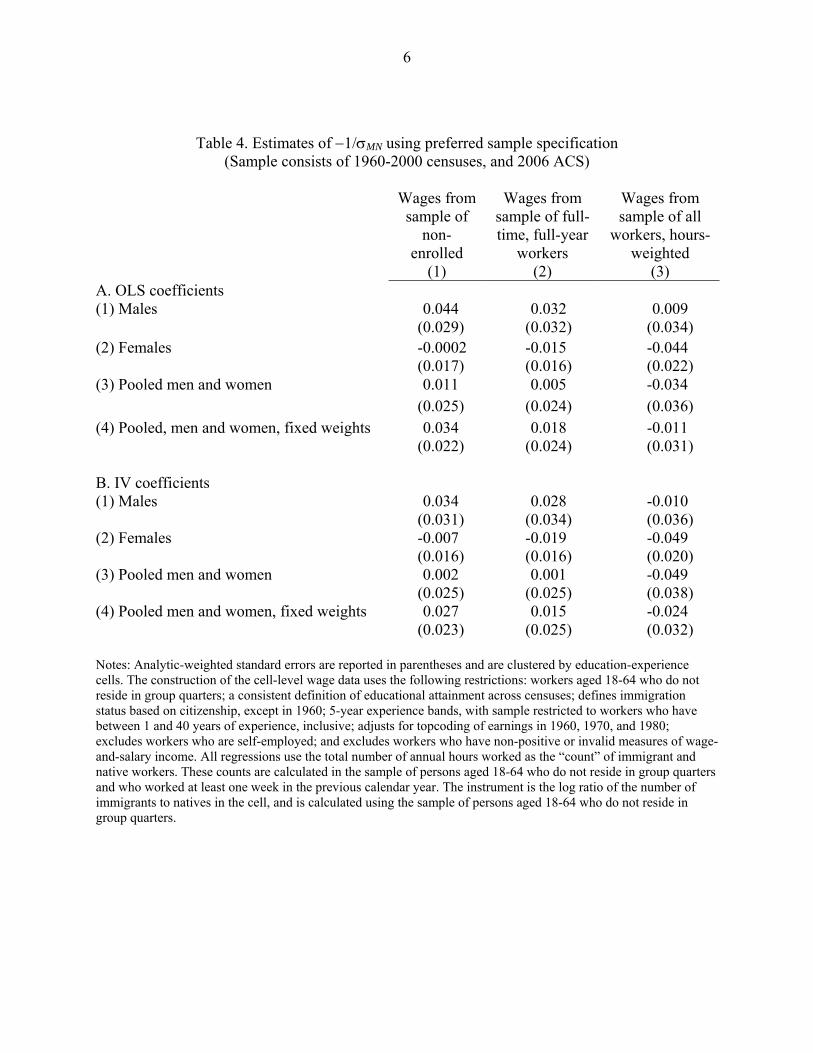
6

Table 4. Estimates of −1/σMN using preferred sample specification (Sample consists of 1960-2000 censuses, and 2006 ACS)

Wages from

sample of non-

enrolled (1)

Wages from sample of full-time, full-year

workers (2)

Wages from sample of all

workers, hours-weighted

(3) A. OLS coefficients (1) Males 0.044 0.032 0.009 (0.029) (0.032) (0.034) (2) Females -0.0002 -0.015 -0.044 (0.017) (0.016) (0.022) (3) Pooled men and women 0.011 0.005 -0.034 (0.025) (0.024) (0.036) (4) Pooled, men and women, fixed weights 0.034 0.018 -0.011 (0.022) (0.024) (0.031) B. IV coefficients

(1) Males 0.034 0.028 -0.010 (0.031) (0.034) (0.036) (2) Females -0.007 -0.019 -0.049 (0.016) (0.016) (0.020) (3) Pooled men and women 0.002 0.001 -0.049 (0.025) (0.025) (0.038) (4) Pooled men and women, fixed weights 0.027 0.015 -0.024 (0.023) (0.025) (0.032) Notes: Analytic-weighted standard errors are reported in parentheses and are clustered by education-experience cells. The construction of the cell-level wage data uses the following restrictions: workers aged 18-64 who do not reside in group quarters; a consistent definition of educational attainment across censuses; defines immigration status based on citizenship, except in 1960; 5-year experience bands, with sample restricted to workers who have between 1 and 40 years of experience, inclusive; adjusts for topcoding of earnings in 1960, 1970, and 1980; excludes workers who are self-employed; and excludes workers who have non-positive or invalid measures of wage-and-salary income. All regressions use the total number of annual hours worked as the “count” of immigrant and native workers. These counts are calculated in the sample of persons aged 18-64 who do not reside in group quarters and who worked at least one week in the previous calendar year. The instrument is the log ratio of the number of immigrants to natives in the cell, and is calculated using the sample of persons aged 18-64 who do not reside in group quarters.

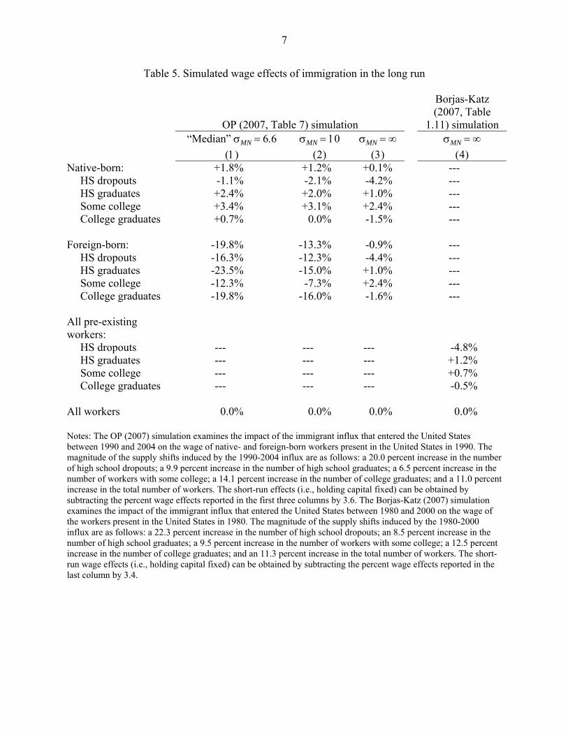
7

Table 5. Simulated wage effects of immigration in the long run

OP (2007, Table 7) simulation

Borjas-Katz (2007, Table

1.11) simulation “Median” σMN = 6.6

(1) σMN = 10

(2) σMN = ∞

(3)

σMN = ∞ (4)

Native-born: +1.8% +1.2% +0.1% --- HS dropouts -1.1% -2.1% -4.2% --- HS graduates +2.4% +2.0% +1.0% --- Some college +3.4% +3.1% +2.4% --- College graduates +0.7% 0.0% -1.5% ---

Foreign-born: -19.8% -13.3% -0.9% ---

HS dropouts -16.3% -12.3% -4.4% --- HS graduates -23.5% -15.0% +1.0% --- Some college -12.3% -7.3% +2.4% --- College graduates -19.8% -16.0% -1.6% ---

All pre-existing workers:

HS dropouts --- --- --- -4.8% HS graduates --- --- --- +1.2% Some college --- --- --- +0.7% College graduates --- --- --- -0.5%

All workers 0.0% 0.0% 0.0% 0.0% Notes: The OP (2007) simulation examines the impact of the immigrant influx that entered the United States between 1990 and 2004 on the wage of native- and foreign-born workers present in the United States in 1990. The magnitude of the supply shifts induced by the 1990-2004 influx are as follows: a 20.0 percent increase in the number of high school dropouts; a 9.9 percent increase in the number of high school graduates; a 6.5 percent increase in the number of workers with some college; a 14.1 percent increase in the number of college graduates; and a 11.0 percent increase in the total number of workers. The short-run effects (i.e., holding capital fixed) can be obtained by subtracting the percent wage effects reported in the first three columns by 3.6. The Borjas-Katz (2007) simulation examines the impact of the immigrant influx that entered the United States between 1980 and 2000 on the wage of the workers present in the United States in 1980. The magnitude of the supply shifts induced by the 1980-2000 influx are as follows: a 22.3 percent increase in the number of high school dropouts; an 8.5 percent increase in the number of high school graduates; a 9.5 percent increase in the number of workers with some college; a 12.5 percent increase in the number of college graduates; and an 11.3 percent increase in the total number of workers. The short-run wage effects (i.e., holding capital fixed) can be obtained by subtracting the percent wage effects reported in the last column by 3.4.