Improved Wide-Angle, Fisheye and OmnidirectionalCamera Calibration

Steffen Urban, Jens Leitloff, Stefan Hinz

Karlsruhe Institute of Technology (KIT), Institute of Photogrammetry and Remote Sensing,Englerstr. 7, 76131 Karlsruhe

Abstract

In this paper an improved method for calibrating wide-angle, fisheye and omni-

directional imaging systems is presented. We extend the calibration procedure

proposed by Scaramuzza et al. by replacing the residual function and joint re-

finement of all parameters. In doing so, we achieve a more stable, robust and

accurate calibration (up to factor 7) and can reduce the number of necessary

calibration steps from five to three. After introducing the camera model and

highlighting the differences from the current calibration procedure, we perform

a comprehensive performance evaluation using several data sets and show the

impact of the proposed calibration procedure on the calibration results.

Keywords: Camera, Calibration, Accuracy, Precision, Geometric, Robotics,

Bundle, Fisheye, Omnidirectional

1. INTRODUCTION

In this paper we extend an existing method to calibrate wide-angle, fisheye

and omnidirectional cameras based on the generalized camera model introduced

in [1]. In the following, we propose contributions that not only enhance the meth-

ods implemented in [2], but also the underlying calibration procedure. Our main

contribution will be the reformulation of the two step non-linear optimization to

∗Corresponding authorEmail address: steffen.urban@kit.edu (Steffen Urban, Jens Leitloff, Stefan Hinz)URL: www.ipf.kit.edu (Steffen Urban, Jens Leitloff, Stefan Hinz)

Preprint submitted to Journal of LATEX Templates March 24, 2015

jointly refine all calibration parameters. We then perform various calibrations

on data sets provided by the authors [2] and own data sets. Afterwards, we

elaborately analyze the results and detail the significant gain in performance

and accuracy. In addition, we calibrated all cameras with another calibration

method proposed by [3] which is also available as a Matlab toolbox [4]. The

Matlab implementation of all proposed contributions as well as test data sets

and evaluation scripts will be made available online1.

1.1. Related Work

Wide-angle, omnidirectional and fisheye cameras are nowadays popular in

many fields of computer vision, robotics and photogrammetric tasks such as

navigation, localization, tracking, mapping and so on. As soon as metric infor-

mation needs to be extracted, camera calibration is the first necessary step to

determine the relation between a 3D ray and its corresponding mapping on the

image plane.

In general, camera calibration consists of two steps. The first involves the

choice of an appropriate model that describes the behavior of the imaging sys-

tem. In recent years various such models for dioptric (fisheye) and catadioptric

(omnidirectional) cameras have been proposed [1, 5, 3, 6, 7, 8]. In [9] a compre-

hensive overview is given. The second step is the estimation of all parameters

that a certain model incorporates, i.e. interior and exterior orientation of the

system as well as distortion parameters that model the differences from an ideal

imaging process. Several methods for calibration have been proposed, that can

be classified into three categories [10] starting with the most general one.

The first is auto- or self-calibration, where epipolar-constraints and point

correspondences between multiple views are used [6, 11, 12]. In [11] the auto-

calibration for fisheye and catadioptric systems is based on the robust estab-

lishment of the epipolar geometry from few correspondences in two images by

solving a polynomial eigenvalue problem. Using this model, Ransac is employed

1http://www.ipf.kit.edu/code.php

2

to remove outliers and no prior knowledge about the scene is necessary. Sub-

sequently, bundle block adjustment can be employed, to estimate all camera

parameters and reconstruct the scene except for a similarity transformation.

The second is space resection of one image from a non-planar object with

known 3D world coordinates [13, 14]. [13] investigate the validity of geometric

projections for fisheye lenses. The camera is calibrated using one image of a

room prepared with 3D-passpoints, that cover the field of view of the fisheye

lens. To enhance the model quality and compensate for real world deviations

from the geometric model, radial as well as tangential distortion parameters are

subsequently added to the projection model. A camera calibration approach for

catadioptric cameras using space resection is proposed in [14]. Lifted coordinates

are used to linearily project scene points to the image plane. After the projection

matrix is estimated from scene points distributed over a 3D-calibration object a

final non-linear refinement is applied.

The third calibration method involves the observation of a planar object

(e.g. checkerboard) with known 3D object coordinates [1, 3, 10] where at least

two images of the planar object are necessary [10]. The calibration procedure

of [3] involves the manual selection of mirror border and center, respectively.

For fisheye lenses the image center is used. The generalized focal length, which

is part of the exact projection model, is estimated from at least three points

on a line. To automatically extract all checkerboard corners, a planar homog-

raphy is estimated from four manually selected points. Then the remaining

checkerboard points are projected to their estimated location and a local sub-

pixel corner search is performed. The initially estimated homography is based

on start values such as the generalized focal length and the center of distor-

tion and thus already imposes model assumptions. If the initial assumptions

are highly biased the subsequent procedure can hardly recover. The projection

model of [3] include tangential distortion parameters, whereas [1] models only

radial symmetric effects. [1] initially extracts all checkerboard corners using the

algorithm of [15]. The calibration procedure is based on multiple observations of

3

a planar calibration object [10], is fully automatic and does not require further

user interaction or prior knowledge. A potential disadvantage are wrong point

extractions, that can bias the calibration result. Also the two-step refinement

of interior and exterior orientation is critical, as all parameters are strongly cor-

related. Our proposed approach tries to avoid both possible disadvantages, but

does not change the underlying projection model.

1.2. Contributions

In this paper we extend and improve the widespread calibration procedure

of [1] and its online available implementation [2] as this does not provide an

optimal solution. The camera model proposed in [1] is general and does not

require prior knowledge about the imaging function. The calibration procedure

is almost fully automatic, online available [2] and is conducted in five consecutive

steps.

We analyzed the two step refinement of interior and exterior orientation and

replaced the employed residual function in order to be able to jointly refine all

parameters. Thereby we obtain better convergence behaviours of the non-linear

least squares optimization and it shows that the original five step calibration

procedure can be conducted in three steps. In addition, we change the original

implementation to a consistent use of subpixel accurate point measurements.

All changes are available online and can be used as an add-on to the original

toolbox at hand.

Previous work for improving [1] was conducted by [16]. They extended the

camera model by replacing the affine transformation between image and sen-

sor plane coordinates with a perspective transformation and also proposed a

new method to estimate the center of distortion. They indicate that a bun-

dle adjustment was performed in the end without providing details. Then they

conducted calibrations on several data sets and compared the results to the orig-

inal implementation. They observed slight improvements of the mean squared

reprojection error (MSE in pixel) but did not discuss why the standard devia-

tion of the reprojection error was partly larger than the MSE and even larger

4

than the standard deviation of the original implementation. Further, only the

reprojection error was investigated to assess the calibration quality. This paper

additionally examines the quality of the estimated calibration parameters.

In the remainder of this paper, we first recapitulate the camera model as well

as the calibration procedure as proposed in [1]. Then, we detail our contributions

to the existing approach and perform a comprehensive evaluation using data sets

provided by the authors [2] as well as own data sets and show that we achieve a

significant accuracy increase. The improved results are subsequently compared

to a different calibration method proposed by [3].

2. Camera Model and Calibration

In the following and for the sake of the self-containedness of this paper, we

include a condensed compilation of the generalized camera model of [1] and the

five consecutive steps that it takes to estimate all model parameters. For a

detailed description and insight we refer to [1],[5]. We use a similar notation as

[1] to facilitate the comparison, i.e. vectors and matrices are typed in boldface,

e.g. R, m, thereby vectors are lowercase and matrices are uppercase. In addition

parameters to be estimated are indicated by a hat, e.g. R, a.

Subsequently, we detail the procedure that is employed to estimate all cal-

ibration related parameters. In Section 3 we propose our improvements to the

given procedure and their implementation.

2.1. Generalized Camera Model

Let m′ = [u′, v′]T be a point on the image plane, i.e. the coordinates are

measured from the upper left corner of the image. Its corresponding point on the

sensor plane, i.e. measured from the image center, is denoted by m = [u, v]T .

Those two points, are related by an affine transformation m′ = Am + Oc:u′v′

=

c d

e 1

uv

+

ouov

(1)

5

The transformation matrix A accounts for small misalignments between sensor

and lens axes and the digitization process. The translation Oc = [ou, ov]T relates

all coordinates to the center of distortion. Now let Xc = [Xc, Yc, Zc]T be a scene

point in the camera coordinate system. Then, the following forward mapping

from a 2D image point to its corresponding 3D ray is described through the

imaging function g.

λg(m) = λ(u, v, f(u, v))T = λ(u, v, f(ρ))T = Xc (2)

with λ > 0 and ρ =√u2 + v2 being the radial euclidean distance from the

image center. Thus, the mapping g is assumed to be rotationally symmetric.

Function f usually depends on the mirror or lens of the system and models the

projection. In literature and practical applications various projection models can

be found (see Section 1.1). Instead of modelling the projection with a specific

mapping function, [1] chose to approximate it with a Taylor expansion making

it applicable for various lenses without prior knowledge:

f(ρ) = a0 + a2ρ2 + ...+ anρ

n (3)

In the next section the calibration procedure is detailed which is aimed at an

accurate estimation of the mapping function g.

2.2. Camera Calibration

For this particular camera model, the goal of calibration is to estimate the

parameters of the imaging function g, i.e. the N − 1 coefficients a0, a2, ..., aN

that describe the shape of the projection function, as well as the parameters of

the affine transformation A and the center of distortion Oc. During the first

calibration steps A is set to be an identity matrix I2,2, thus the eccentricity

of the mirror boundary is set to 0. The inital estimate of the center of distor-

tion Oc is always set to the image center. During camera calibration, a planar

calibration pattern (Zi = 0) is observed j = 1, ..,K times from an unknown

position Pj = [r1, r2, r3, t]j . The i = 1, .., L object coordinates are denoted by

6

Xi =[Xi, Yi, 0, 1

]T. The corresponding image points mij = [u′ij − ou, v′ij − ov]T

are extracted in each image. This leads to the following relation:

λijg(m)ij = λij

u

v

a0, .., aNρN

ij

= PjXi =[r1 r2 t

]j

X

Y

1

i

(4)

Observe that the third column vector r3 of P is omitted because Zi = 0.

2.2.1. Linear Estimation of the Exterior and Iinterior Orientation

In order to solve Eq. 4 for all interior orientation parameters, the K exterior

orientations are estimated in advance. First the scale factor λ is eliminated

for each equation by vectorially multiplying both sides of Eq. 4 with g(m)ij

yielding: vi(r31Xi + r32Yi + t3)− f(ρi)(r21Xi + r22Yi + t2)

f(ρi)(r11Xi + r12Yi + t1)− ui(r31Xi + r32Yi + t3)

ui(r21Xi + r22Yi + t2)− vi(r11Xi + r12Yi + t1)

= 0 (5)

Then, and since Xi, Yi, ui, vi are the known observations, the third equation

which is linear in all unknowns and does not depend on f , can be used to get

an initial estimate of the parameters of the exterior orientation. Subsequently,

latter are substituted into Eq. 5 and the resulting system is solved for the

interior orientation parameters. At this point a linear estimate of all involved

parameters, i.e. U = [R, T, a0, a2, ..., aN ]T is found.

2.2.2. Center of Distortion

Until now the linear calibration procedure is carried out with the assump-

tions that the image center is identical to the center of distortion. To find a

better estimate of the center, [5] carry out an iterative search procedure, prior

to performing the non-linear refinement of all parameters. First a regular grid

is placed over the image around a given Oc, where each grid point corresponds

to a potential Oc. Then a the linear calibration procedure is conducted for each

grid point and the Sum of Squared Reprojection Errors (SSRE) is calculated.

7

The grid point with the minimum SSRE is taken as the potential Oc and the

process is repeated until the change between two potential Oc is less than 0.5

pixels ([5]).

2.2.3. Linear Refinement of Exterior and Interior Orientation

Finally the linear estimation of interior and exterior orientation is conducted

once more with the updated center point Oc, yielding the initial start values for

the two-step non-linear refinement with all parameters.

2.2.4. Two-Step Non-linear Refinement

The last step in the calibration procedure of [5] is a non-linear refinement

involving all calibration parameters, i.e. the exterior orientation of each camera

w.r.t the calibration pattern as well as the interior orientation parameters. In-

stead of jointly optimizing all parameters, [5] split the estimation in two steps,

i.e. interior and exterior orientation are estimated separately. They state that

the convergence is not affected but the runtime is decreased. The following

residual is calculated for each point correspondence:

rs(m′, m′) =

√(u′ − u′)2 + (v′ − v′)2 (6)

and the non-linear least squares problem is solved:

1. Exterior orientation

In a first step the exterior orientation of all camera poses is optimized.

The interior orientation parameters are fixed to the values obtained from

the last linear estimation, thus:

minP‖rs‖2 = min

P

K∑j=1

L∑i=1

rs(m′ij , m

′ij(P,a,A,Oc,X))2 (7)

where a = [a0, a2, ..., aN ] are the polynomial coefficients. The affine matrix

A is initialized with the identity matrix for the first iteration.

2. Interior orientation

Now the exterior orientation is fixed to the values from the previous step

8

and the interior orientation is refined, thus

mina,A,Oc

‖rs‖2 = mina,A,Oc

K∑j=1

L∑i=1

rs(m′ij , m

′ij(P, a, A, Oc,X))2 (8)

Observe also, that the affine matrix A is now estimated for the first time.

3. Proposed Camera Calibration

3.1. Analysis of the Two-Step Non-Linear Refinement

We conducted various test calibrations with different data sets and iteratively

repeated the two step refinement proposed in [5], but could not reproduce a

converging solution. After each iteration, we calculate the RMS (root mean

square):

RMS =

√∑ni=1 ‖(m′i − m′i)‖2

2n(9)

where n is the total number of point correspondences over all images.

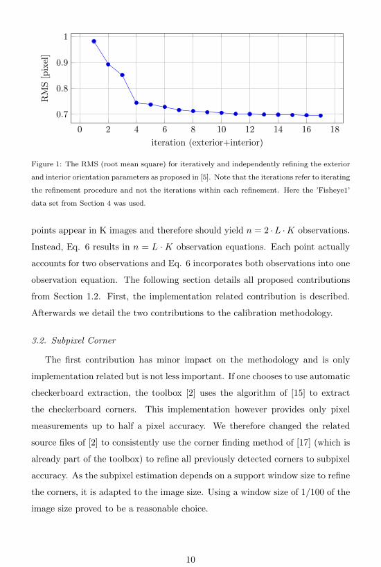
Figure 1 depicts the effect of alternately refining exterior and interior orien-

tation for the ’Fisheye1’ data set (see Section 4), i.e. each iteration represents

the result of one two-step refinement as detailed in the previous chapter. The

result of each iteration is used for the next iteration. This example shows, that

the iterative two-step procedure would not even stop after the 17-th iteration

as the error still decreases. Moreover the RMS after the 17-th iteration is still

above our, in the following presented method (compare to Table 1).

As one set of the parameters (Eq. 7: A,a,Oc) is always fixed while the other

set of parameters (Eq. 7: P) is optimized and the RMS value is still decreasing,

it is very likely that these two sets of parameters are correlated, i.e. it is unlikely

that the algorithm will converge to a correct minimum by alternating Eq. 7 and

Eq. 8. We also observed, that the two-step refinement yielded slightly different

results (e.g. in the order of pixels for the principal point) for slightly different

initial distortion centers. This indicates, that a global minimum is not attained.

Considering again Eq. 7 and Eq. 8 and the respective residual function Eq.

6, we can observe a potential disadvantage of the proposed error function. L

9

0 2 4 6 8 10 12 14 16 18

0.7

0.8

0.9

1

iteration (exterior+interior)

RM

S[p

ixel

]

Figure 1: The RMS (root mean square) for iteratively and independently refining the exterior

and interior orientation parameters as proposed in [5]. Note that the iterations refer to iterating

the refinement procedure and not the iterations within each refinement. Here the ’Fisheye1’

data set from Section 4 was used.

points appear in K images and therefore should yield n = 2 ·L ·K observations.

Instead, Eq. 6 results in n = L ·K observation equations. Each point actually

accounts for two observations and Eq. 6 incorporates both observations into one

observation equation. The following section details all proposed contributions

from Section 1.2. First, the implementation related contribution is described.

Afterwards we detail the two contributions to the calibration methodology.

3.2. Subpixel Corner

The first contribution has minor impact on the methodology and is only

implementation related but is not less important. If one chooses to use automatic

checkerboard extraction, the toolbox [2] uses the algorithm of [15] to extract

the checkerboard corners. This implementation however provides only pixel

measurements up to half a pixel accuracy. We therefore changed the related

source files of [2] to consistently use the corner finding method of [17] (which is

already part of the toolbox) to refine all previously detected corners to subpixel

accuracy. As the subpixel estimation depends on a support window size to refine

the corners, it is adapted to the image size. Using a window size of 1/100 of the

image size proved to be a reasonable choice.

10

3.3. Non-linear Refinement

Instead of using the original two-step optimization method of [5], we propose

a method that jointly refines all calibration parameters. Using the image center,

together with the linear estimated parameters obtained in Section 2.2 as initial

values is sufficient for the non-linear least squares minimization to converge

quickly.

The first step is to reformulate Eq. 6 and introduce a different residual

function that lets us fully exploit the information at each point:

rnew(m′, m′, k) = m′k − m′k (10)

where k = 1, 2 is either the u′ or the v′ component of the coordinate pair m′.

Now we can substitute Eq. 10 to Eq. 7 or Eq. 8 respectively which now yields

n = 2 · L ·K observation equations:

minU‖rnew‖2 = min

U

K∑j=1

L∑i=1

2∑k=1

rnew(m′ij , m′ij(U,X), k)2 (11)

with U = [P, a, A, Oc] being the parameter vector. Following the original im-

plementation, we minimize the non-linear least squares problem Eq. 11 using

Matlab’s lsqnonlin function.

At first glance, the expanded observation equations Eq. 7 and Eq. 11 should

be equal. The major difference lies in the residual function and the resulting

normal equations. As emphasized in Section 3.1, the original residual frunction

incorporates both observations of one image point into one observation equation.

Hence the finite differencing step of lsqnonlin leads to different derivations at

the point of the respective unknowns. In addition, the original residual function

Eq. 6 is not differentiable at the point of zero residual.

Performing several calibrations with different data sets (see Section 4) has

shown, that the search for the center of distortion can be completely omitted,

since the global minimum of all parameters is always found. We hereby reduce

the number of necessary calibration steps to three, i.e. linear estimation of

exterior and interior orientation and non-linear refinement of all parameters.

11

Furthermore, the total runtime of the calibration procedure decreases as well

(see Section 4.3), although the runtime of the proposed one step refinement is

slightly higher than the two step refinement. Besides, latter is only true if the

two step refinement is carried out only once. To obtain an adequate calibration

with [5] the two step procedure has to be iterated multiple times.

3.4. Robust Non-linear Refinement

Usually it is not necessary to apply a robust optimization method to camera

calibration. But by analyzing the extracted points from [15] we found that wrong

corner points are extracted from time to time. Figure 2 depicts an example.

Instead of leaving the removal of such points up to the user, we can downweight

their influence during iterative application of the non-linear optimization and

treat them as outliers. We do that by applying a robust M-estimator to our

proposed method and performing iterative reweighted least squares:

minU‖rnew‖2 = min

U

K∑j=1

L∑i=1

2∑k=1

ωc(rnewh−1)rnew(m′ij , m

′ij(U,X), k)2 (12)

where the superscript h indicates the h-th iteration. For the weight function ω

we chose Huber’s function:

ωc(r) =

1, |r| ≤ c

c/|r|, |r| > c. (13)

with c = 1 is the tuning constant. For residuals below 1 pixel the function

behaves like normal least squares. All pixels with residuals larger than 1 pixel

get downweighted.

4. Performance Evaluation

In the following, we evaluate the impact of the contributions on the calibra-

tion results. In order to provide a comprehensive evaluation, images provided by

[2] containing omnidirectional and fisheye cameras as well as three own data sets

of fisheye and wide-angle cameras are used. We hereby covered different camera

12

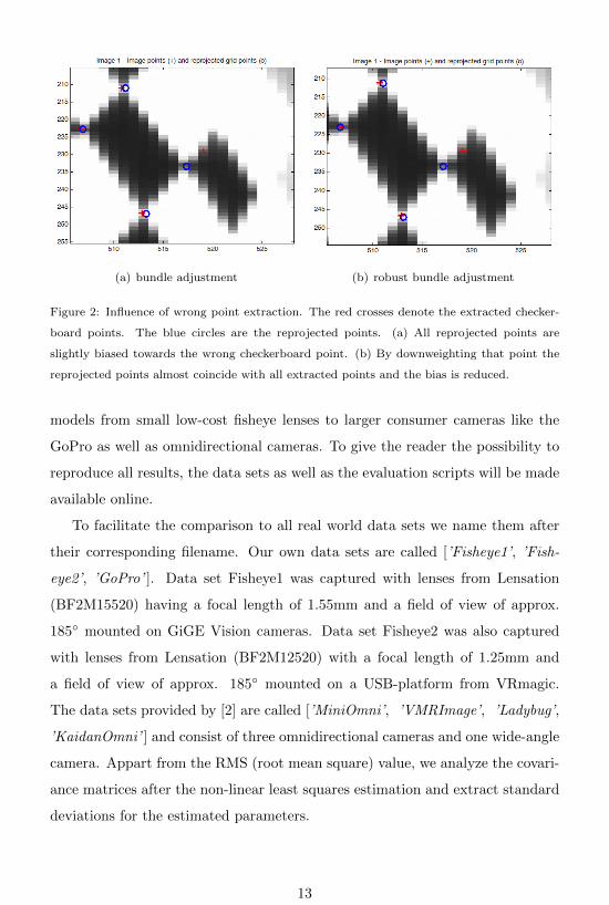
(a) bundle adjustment (b) robust bundle adjustment

Figure 2: Influence of wrong point extraction. The red crosses denote the extracted checker-

board points. The blue circles are the reprojected points. (a) All reprojected points are

slightly biased towards the wrong checkerboard point. (b) By downweighting that point the

reprojected points almost coincide with all extracted points and the bias is reduced.

models from small low-cost fisheye lenses to larger consumer cameras like the

GoPro as well as omnidirectional cameras. To give the reader the possibility to

reproduce all results, the data sets as well as the evaluation scripts will be made

available online.

To facilitate the comparison to all real world data sets we name them after

their corresponding filename. Our own data sets are called [’Fisheye1’, ’Fish-

eye2’, ’GoPro’ ]. Data set Fisheye1 was captured with lenses from Lensation

(BF2M15520) having a focal length of 1.55mm and a field of view of approx.

185◦ mounted on GiGE Vision cameras. Data set Fisheye2 was also captured

with lenses from Lensation (BF2M12520) with a focal length of 1.25mm and

a field of view of approx. 185◦ mounted on a USB-platform from VRmagic.

The data sets provided by [2] are called [’MiniOmni’, ’VMRImage’, ’Ladybug’,

’KaidanOmni’ ] and consist of three omnidirectional cameras and one wide-angle

camera. Appart from the RMS (root mean square) value, we analyze the covari-

ance matrices after the non-linear least squares estimation and extract standard

deviations for the estimated parameters.

13

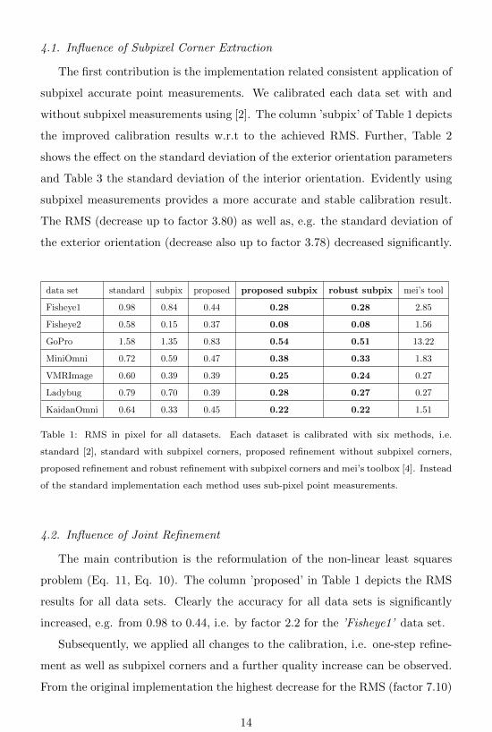
4.1. Influence of Subpixel Corner Extraction

The first contribution is the implementation related consistent application of

subpixel accurate point measurements. We calibrated each data set with and

without subpixel measurements using [2]. The column ’subpix’ of Table 1 depicts

the improved calibration results w.r.t to the achieved RMS. Further, Table 2

shows the effect on the standard deviation of the exterior orientation parameters

and Table 3 the standard deviation of the interior orientation. Evidently using

subpixel measurements provides a more accurate and stable calibration result.

The RMS (decrease up to factor 3.80) as well as, e.g. the standard deviation of

the exterior orientation (decrease also up to factor 3.78) decreased significantly.

data set standard subpix proposed proposed subpix robust subpix mei’s tool

Fisheye1 0.98 0.84 0.44 0.28 0.28 2.85

Fisheye2 0.58 0.15 0.37 0.08 0.08 1.56

GoPro 1.58 1.35 0.83 0.54 0.51 13.22

MiniOmni 0.72 0.59 0.47 0.38 0.33 1.83

VMRImage 0.60 0.39 0.39 0.25 0.24 0.27

Ladybug 0.79 0.70 0.39 0.28 0.27 0.27

KaidanOmni 0.64 0.33 0.45 0.22 0.22 1.51

Table 1: RMS in pixel for all datasets. Each dataset is calibrated with six methods, i.e.

standard [2], standard with subpixel corners, proposed refinement without subpixel corners,

proposed refinement and robust refinement with subpixel corners and mei’s toolbox [4]. Instead

of the standard implementation each method uses sub-pixel point measurements.

4.2. Influence of Joint Refinement

The main contribution is the reformulation of the non-linear least squares

problem (Eq. 11, Eq. 10). The column ’proposed’ in Table 1 depicts the RMS

results for all data sets. Clearly the accuracy for all data sets is significantly

increased, e.g. from 0.98 to 0.44, i.e. by factor 2.2 for the ’Fisheye1’ data set.

Subsequently, we applied all changes to the calibration, i.e. one-step refine-

ment as well as subpixel corners and a further quality increase can be observed.

From the original implementation the highest decrease for the RMS (factor 7.10)

14

can be observed for the ’Fisheye2’ data set. Furthermore, for all data sets that

contained outlier corners, i.e. where a reprojected point does not lie within

the radius of 1 pixel from the extracted checkerboard corner, the robust bundle

adjustment yielded even better results. From Table 1 we can derive a mean

RMS decrease for each column compared to the standard implementation. The

mean RMS decrease to ’subpix’ is 1.27, to ’proposed’ it’s 1.75, to ’proposed sub-

pix’ it’s 3.37 and to ’robust subpix’ it’s 3.45. This proofs the validity of each

contribution. The overall performance gain for the RMS between the standard

implementation [2] and our proposed method is also graphically visualized in

Figure 3.

As the RMS is only an indication of how well the estimated model describes

the observations, we also assessed the quality of the estimated parameters. Since

the redundancy of our proposed bundle adjustment is large, we can calculate the

empirical covariance matrix Σxx [18]. The main diagonal of Σxx contains the

variance information of all unknowns parameters U. As the standard implemen-

tation separates the refinement into two steps, we extract one covariance matrix

after each step separately, i.e. yielding a covariance matrix for interior and ex-

terior orientation. Note, that the separated covariance matrices do not contain

the aforementioned correlations between the calibration parameters. This sta-

tistical fact additionally reveals the disadvantage of refining interior and exterior

orientation separately. Hence, a comparison of the covariance matrices between

the standard and our proposed approach should only be cautiously interpreted.

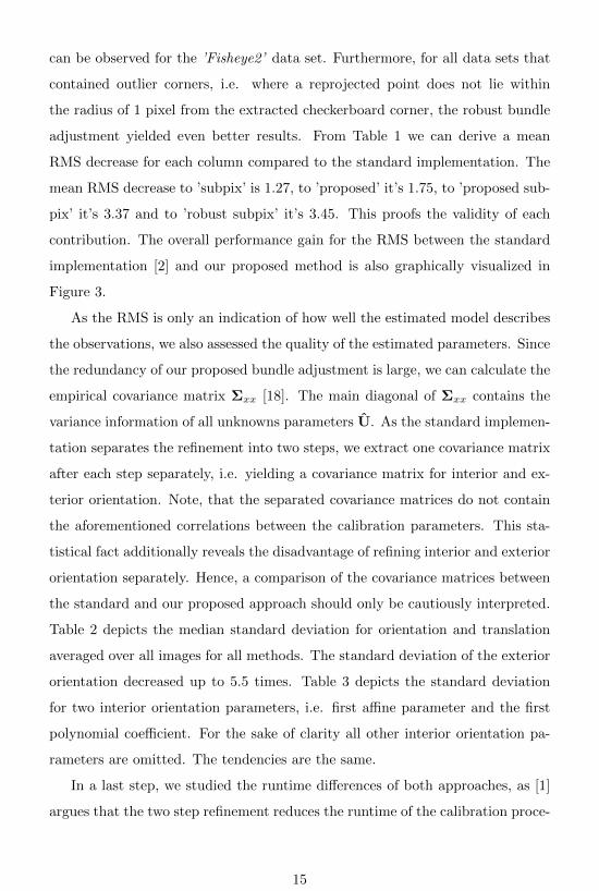
Table 2 depicts the median standard deviation for orientation and translation

averaged over all images for all methods. The standard deviation of the exterior

orientation decreased up to 5.5 times. Table 3 depicts the standard deviation

for two interior orientation parameters, i.e. first affine parameter and the first

polynomial coefficient. For the sake of clarity all other interior orientation pa-

rameters are omitted. The tendencies are the same.

In a last step, we studied the runtime differences of both approaches, as [1]

argues that the two step refinement reduces the runtime of the calibration proce-

15

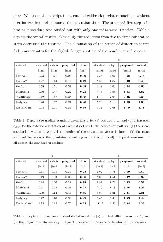
dure. We assembled a script to execute all calibration related functions without

user interaction and measured the execution time. The standard five step cali-

bration procedure was carried out with only one refinement iteration. Table 4

depicts the overall results. Obviously the reduction from five to three calibration

steps decreased the runtime. The elimination of the center of distortion search

fully compensates for the slightly longer runtime of the non-linear refinement.

(a)

data set standard subpix proposed robust

[mm] [mm] [mm] [mm]

Fisheye1 0.23 0.21 0.09 0.09

Fisheye2 1.27 0.34 0.19 0.19

GoPro 0.58 0.51 0.39 0.38

MiniOmni 0.56 0.47 0.27 0.23

VMRImage 0.42 0.27 0.38 0.38

Ladybug 0.26 0.22 0.27 0.26

KaidanOmni 0.63 0.31 0.39 0.39

(b)

standard subpix proposed robust

[mrad] [mrad] [mrad] [mrad]

2.36 2.07 0.68 0.73

2.39 0.87 0.40 0.40

1.12 1.00 0.64 0.63

4.77 3.93 1.83 1.62

6.19 3.95 2.36 2.35

3.23 3.18 1.68 1.63

5.24 2.68 1.79 1.78

Table 2: Depicts the median standard deviations σ for (a) position σxyz and (b) orientation

σφκγ for the exterior orientation of each dataset w.r.t. the calibration pattern. (a) the mean

standard deviation in x,y and z direction of the translation vector in [mm]. (b) the mean

standard deviation of the orientation about x,y and z axis in [mrad]. Subpixel were used for

all exepct the standard procedure.

(a)

data set standard subpix proposed robust

[1e-3] [1e-3] [1e-3] [1e-3]

Fisheye1 0.41 0.35 0.13 0.23

Fisheye2 0.49 0.13 0.08 0.08

GoPro 0.24 0.20 0.18 0.18

MiniOmni 0.41 0.33 0.26 0.23

VMRImage 0.39 0.24 0.45 0.45

Ladybug 0.72 0.60 0.30 0.29

KaidanOmni 1.72 0.83 0.72 0.72

(b)

standard subpix proposed robust

[1e-3] [1e-3] [1e-3] [1e-3]

2.02 1.71 0.69 0.69

2.06 0.51 0.32 0.32

0.92 0.79 0.53 0.52

7.30 6.13 3.66 3.27

5.28 3.21 2.31 2.31

2.65 2.40 1.53 1.48

18.47 8.59 5.24 5.22

Table 3: Depicts the median standard deviations σ for (a) the first affine parameter σc and

(b) the polynom coefficient σa0 . Subpixel were used for all except the standard procedure.

16

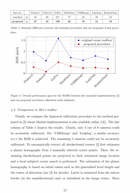
data set: Fisheye1 Fisheye2 GoPro MiniOmni VMRImage Ladybug KaidanOmni

standard [s] 48 68 211 77 35 28 32

proposed [s] 37 43 196 58 18 12 18

Table 4: Runtime difference between the standard procedure and our proposed 3-step proce-

dure.

Fishey

e1

Fishey

e2

GoP

ro

Min

iOm

ni

VM

RIm

age

Ladyb

ug

Kaida

nOm

ni0

0.5

1

1.5

RM

S[p

ixel

]

original ocam toolboxproposed procedure

Figure 3: Overall performance gain for the RMSE between the standard implementation [2]

and our proposed non-linear refinement with subpixels.

4.3. Comparison to Mei’s toolbox

Finally, we compare the improved calibration procedure to the method pro-

posed in [3] whose Matlab implementation is also available online ([4]). The last

column of Table 1 depicts the results. Clearly, only 3 out of 8 cameras could

be accurately calibrated. For ’VMRImage’ and ’Ladybug’, a similar accuracy

w.r.t the RMS is achievied. The remaining 5 cameras could not be accurately

calibrated. To automatically extract all checkerboard corners [3] first estimates

a planar homography from 4 manually selected corner points. Then, the re-

maining checkerboard points are projected to their estimated image location

and a local subpixel corner search is performed. The estimation of the planar

homography is based on initial values such as the generalized focal length and

the center of distortion (see [3] for details). Latter is estimated from the mirror

border (in the omnidirectional case) or initialized as the image center. Since

17

some of the cameras are low-cost and the center of distortion can have a large

offset to the image center, the initial estimates are significantly biased and the

calibration procedure can obviously not recover from that. This is confirmed

by the fact, that we were not able to accurately calibrate our fisheye cameras

’Fisheye1’, ’Fisheye2’. For both cameras the center of distortion deviates more

than 10 pixels from the image center. After performing several calibrations on

all data sets, we found that a large percentage of points are falsely extracted.

For some data sets, we improved the calibration result by manual tuning of the

search window of the subpixel corner search or by using better initial estimates,

e.g. for the center of distortion but this is not desirable in the sense of a fully

automatic calibration routine. Note, that our proposed calibration procedure

does not depend on any manual interaction.

5. Conclusions

In this paper, we extended the widely used method and implementation for

fisheye and omnidirectional camera calibration of [1, 2, 5]. Apart from using sub-

pixel accurate corner measurements we reformulated the non-linear least squares

refinement and applied a residual function that allows to jointly optimize all cali-

bration parameters. We further reduced the necessary calibration steps to three

and evaluated the results with various data sets including wide-angle, fisheye

and omnidirectional imaging systems. It showed that a significant performance

increase (RMS up to factor 7.1) could be achieved. Since the automatic corner

extraction yields false locations from time to time, we extended the non-linear re-

finement with an M-estimator to make it robust against outliers. Finally, Figure

4 depicts a visual comparison of the reprojected corners between the standard

method on the left side and our proposed method on the right. Evidently, after a

calibration with the proposed method, the reprojected points (magenta circles)

coincide much better with the extracted corner points (red crosses). A Matlab

implementation of all contributions is available online (see Section 1) and can

be used as an addon to the existing toolbox [2].

18

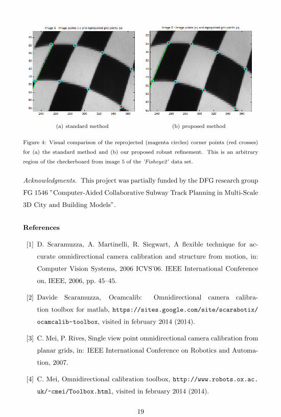
(a) standard method (b) proposed method

Figure 4: Visual comparison of the reprojected (magenta circles) corner points (red crosses)

for (a) the standard method and (b) our proposed robust refinement. This is an arbitrary

region of the checkerboard from image 5 of the ’Fisheye2’ data set.

Acknowledgments. This project was partially funded by the DFG research group

FG 1546 ”Computer-Aided Collaborative Subway Track Planning in Multi-Scale

3D City and Building Models”.

References

[1] D. Scaramuzza, A. Martinelli, R. Siegwart, A flexible technique for ac-

curate omnidirectional camera calibration and structure from motion, in:

Computer Vision Systems, 2006 ICVS’06. IEEE International Conference

on, IEEE, 2006, pp. 45–45.

[2] Davide Scaramuzza, Ocamcalib: Omnidirectional camera calibra-

tion toolbox for matlab, https://sites.google.com/site/scarabotix/

ocamcalib-toolbox, visited in february 2014 (2014).

[3] C. Mei, P. Rives, Single view point omnidirectional camera calibration from

planar grids, in: IEEE International Conference on Robotics and Automa-

tion, 2007.

[4] C. Mei, Omnidirectional calibration toolbox, http://www.robots.ox.ac.

uk/~cmei/Toolbox.html, visited in february 2014 (2014).

19

[5] D. Scaramuzza, A. Martinelli, R. Siegwart, A toolbox for easily calibrat-

ing omnidirectional cameras, in: Intelligent Robots and Systems, 2006

IEEE/RSJ International Conference on, IEEE, 2006, pp. 5695–5701.

[6] B. Micusık, Two-view geometry of omnidirectional cameras, Ph.D. thesis,

Czech Technical University (2004).

[7] J. Kannala, S. S. Brandt, A generic camera model and calibration method

for conventional, wide-angle, and fish-eye lenses, Pattern Analysis and Ma-

chine Intelligence, IEEE Transactions on 28 (8) (2006) 1335–1340.

[8] C. Geyer, K. Daniilidis, A unifying theory for central panoramic systems

and practical implications, in: Computer VisionECCV 2000, Springer, 2000,

pp. 445–461.

[9] L. Puig, J. Bermudez, P. Sturm, J. Guerrero, Calibration of om-

nidirectional cameras in practice: A comparison of methods, Com-

puter Vision and Image Understanding 116 (1) (2012) 120 – 137.

doi:http://dx.doi.org/10.1016/j.cviu.2011.08.003.

URL http://www.sciencedirect.com/science/article/pii/

S1077314211001858

[10] Z. Zhang, Flexible camera calibration by viewing a plane from unknown

orientations, in: Computer Vision, 1999. The Proceedings of the Seventh

IEEE International Conference on, Vol. 1, IEEE, 1999, pp. 666–673.

[11] B. Micusık, T. Pajdla, Structure from motion with wide circular field of view

cameras, Pattern Analysis and Machine Intelligence, IEEE Transactions on

28 (7) (2006) 1135–1149.

[12] O. D. Faugeras, Q.-T. Luong, S. J. Maybank, Camera self-calibration: The-

ory and experiments, in: Computer VisionECCV’92, Springer, 1992, pp.

321–334.

20

[13] D. Schneider, E. Schwalbe, H.-G. Maas, Validation of geometric models

for fisheye lenses, ISPRS Journal of Photogrammetry and Remote Sensing

64 (3) (2009) 259–266.

[14] L. Puig, Y. Bastanlar, P. Sturm, J. J. Guerrero, J. Barreto, Calibration of

central catadioptric cameras using a dlt-like approach, International Journal

of Computer Vision 93 (1) (2011) 101–114.

[15] M. Rufli, D. Scaramuzza, R. Siegwart, Automatic detection of checker-

boards on blurred and distorted images, in: Intelligent Robots and Systems,

2008. IROS 2008. IEEE/RSJ International Conference on, IEEE, 2008, pp.

3121–3126.

[16] O. Frank, R. Katz, C.-L. Tisse, H. F. Durrant-Whyte, Camera calibration

for miniature, low-cost, wide-angle imaging systems., in: BMVC, Citeseer,

2007, pp. 1–10.

[17] J. Bouguet, Camera calibration toolbox for matlab, http:

//www.vision.caltech.edu/bouguetj/calib_doc/index.html, vis-

ited february 2014 [cited 26.02.2014].

URL http://www.vision.caltech.edu/bouguetj/calib_doc/index.

html

[18] C. D. Ghilani, Adjustment computations: spatial data analysis, John Wiley

& Sons, 2010.

21