Embed Size (px)
Citation preview
IMPROVING BATCH REACTORS USING ATTAINABLE REGIONS: TOWARDSAUTOMATED CONSTRUCTION OF THE ATTAINABLE REGION AND ITSAPPLICATION TO BATCH REACTORS
David Ming
A thesis submitted to the Faculty of Engineering and the Built Environment, Universityof the Witwatersrand, Johannesburg, in fulfillment of the requirements for the degreeof Doctor of Philosophy in Engineering.
Johannesburg, 2014

Declaration
I declare that this thesis is my own unaided work. It is being submitted for the
degree Doctor of Philosophy in Engineering to the University of the Witwatersrand,
Johannesburg. It has not been submitted before for any degree or examination to
any other university.
David Ming
day of year
i
Abstract
The Attainable Region is the set of all achievable states, for all possible reactorconfigurations, obtained by reaction and mixing alone. It is a geometric methodthat is effective in addressing problems found in reactor network synthesis. For thisreason, Attainable Region theory assists towards a better understanding of systemsof complex reaction networks and the issues encountered by these systems.
This thesis aims to address two areas in Attainable Region theory:
1. To help improve the design and operation of batch reactors using AttainableRegions.
2. To further advance knowledge and understanding of efficient Attainable Regionconstruction methods.
Using fundamental concepts of mixing and attainability established by AttainableRegion theory, a graphical method of identifying opportunities for improving theproduction rate from batch reactors is first presented. It is found that by modi-fying the initial concentration of the batch, overall production performance maybe improved. This may be achieved in practice by retaining a fraction of the finalproduct volume and mixing with fresh feed material for subsequent cycles. This res-ult is counter-intuitive to the normal method of batch operation. Bypassing of feedmay also be used to improve production rate for exit concentrations not associatedwith the optimal concentration. The graphical approach also allows optimisation ofbatches where only experimental data are given.
An improved method of candidate Attainable Region construction, based onan existing bounding hyperplanes approach is then presented. The method uses aplane rotation about existing extreme points to eliminate unachievable regions froman initial bounding set. The algorithm is shown to be faster and has been extendedto include construction of candidate Attainable Regions involving non-isothermalkinetics in concentration and concentration-time space.
With the ideas obtained above, the application of Attainable Regions to batchreactor configurations is finally presented. It is shown that with the appropriatetransformation, results developed from a continuous Attainable Region may be usedto form a related batch structure. Thus, improvement of batch reactor structures isalso possible using Attainable Regions. Validation of candidate Attainable Regionsis carried out with the construction algorithm developed in this work.
ii

To my parentsChuck and Loraine
To Michelle

Acknowledgements
I would like to thank my supervisors, Professor David Glasser and Professor DianeHildebrandt, for their knowledge, encouragement and guidance over the years. Iknow that many students tend to thank their supervisors at the end of a good re-search meeting. I am still not sure how many of those supervisors acknowledge thestatement and follow up with a thank you of their own. I have enjoyed working withboth of you very much.
I would also like to thank Professor Benjamin Glasser for acting as my surrog-ate supervisor and mentor during the final stages of this work. You were never tooshy to ‘crack the whip’ to ensure that I kept going, but you always did it in a politeway. I am grateful for your guidance and knowledge as well. Thank you.
I would like to thank the University of the Witwatersrand, the National ResearchFoundation and the Centre of Materials and Process Synthesis (currently known asMaPS) for their support.
iv
Contents
Declaration . . . . . . . . . . . . . . . . . . . . . . . . . . . . . . . . . . . iAbstract . . . . . . . . . . . . . . . . . . . . . . . . . . . . . . . . . . . . . iiAcknowledgements . . . . . . . . . . . . . . . . . . . . . . . . . . . . . . . ivList of figures . . . . . . . . . . . . . . . . . . . . . . . . . . . . . . . . . . xList of tables . . . . . . . . . . . . . . . . . . . . . . . . . . . . . . . . . . xiNomenclature . . . . . . . . . . . . . . . . . . . . . . . . . . . . . . . . . . xiii
1 Introduction and literature review 11.1 Introduction . . . . . . . . . . . . . . . . . . . . . . . . . . . . . . . . 11.2 Literature review . . . . . . . . . . . . . . . . . . . . . . . . . . . . . 3
1.2.1 The Attainable Region (AR) . . . . . . . . . . . . . . . . . . 31.2.2 Batch optimisation . . . . . . . . . . . . . . . . . . . . . . . . 11
1.3 Motivation . . . . . . . . . . . . . . . . . . . . . . . . . . . . . . . . 181.3.1 AR construction algorithms . . . . . . . . . . . . . . . . . . . 181.3.2 Batch reactors . . . . . . . . . . . . . . . . . . . . . . . . . . 19
1.4 Conclusion and scope of this work . . . . . . . . . . . . . . . . . . . 201.5 Copyright permissions . . . . . . . . . . . . . . . . . . . . . . . . . . 21
2 Preliminaries 282.1 The Attainable Region . . . . . . . . . . . . . . . . . . . . . . . . . . 282.2 Concentration, mixing and reaction . . . . . . . . . . . . . . . . . . . 28
2.2.1 Concentration . . . . . . . . . . . . . . . . . . . . . . . . . . . 282.2.2 Mixing . . . . . . . . . . . . . . . . . . . . . . . . . . . . . . . 292.2.3 Concavities and mixing . . . . . . . . . . . . . . . . . . . . . 302.2.4 Convex Hulls . . . . . . . . . . . . . . . . . . . . . . . . . . . 312.2.5 Rate vectors and rate fields . . . . . . . . . . . . . . . . . . . 32
2.3 Fundamental reactor types . . . . . . . . . . . . . . . . . . . . . . . . 322.3.1 The Plug Flow Reactor (PFR) . . . . . . . . . . . . . . . . . 322.3.2 The Continuously-Stirred Tank Reactor (CSTR) . . . . . . . 342.3.3 The Differential Side-stream Reactor (DSR) . . . . . . . . . . 35
2.4 Higher dimensional considerations . . . . . . . . . . . . . . . . . . . 372.4.1 Dimension of the AR . . . . . . . . . . . . . . . . . . . . . . . 372.4.2 Stoichiometric subspace . . . . . . . . . . . . . . . . . . . . . 37
v
2.4.3 PFRs on the AR boundary . . . . . . . . . . . . . . . . . . . 382.4.4 Connectors and critical reactors . . . . . . . . . . . . . . . . . 392.4.5 Simplifications for R3 . . . . . . . . . . . . . . . . . . . . . . 43
2.5 AR construction guidelines . . . . . . . . . . . . . . . . . . . . . . . 442.5.1 General procedure for constructing the AR . . . . . . . . . . 442.5.2 Remarks . . . . . . . . . . . . . . . . . . . . . . . . . . . . . . 47
2.6 On non-isothermal and heterogeneous systems . . . . . . . . . . . . . 472.6.1 Variable density systems . . . . . . . . . . . . . . . . . . . . . 472.6.2 Temperature and other parameters . . . . . . . . . . . . . . . 50
2.7 Conclusion . . . . . . . . . . . . . . . . . . . . . . . . . . . . . . . . 51
3 Graphically improving batch production rate 533.1 Introduction . . . . . . . . . . . . . . . . . . . . . . . . . . . . . . . . 533.2 Standard batch operation . . . . . . . . . . . . . . . . . . . . . . . . 54
3.2.1 Problem formulation . . . . . . . . . . . . . . . . . . . . . . . 543.2.2 Initial observations and modifications . . . . . . . . . . . . . 56
3.3 Improving production rate . . . . . . . . . . . . . . . . . . . . . . . . 583.3.1 Improvement 1: Partial emptying and filling . . . . . . . . . . 583.3.2 Improvement 2: Improving production rates for other exit con-
centrations . . . . . . . . . . . . . . . . . . . . . . . . . . . . 623.3.3 Experimental data . . . . . . . . . . . . . . . . . . . . . . . . 643.3.4 Method . . . . . . . . . . . . . . . . . . . . . . . . . . . . . . 65
3.4 Examples . . . . . . . . . . . . . . . . . . . . . . . . . . . . . . . . . 663.4.1 Hydrolysis of propylene oxide . . . . . . . . . . . . . . . . . . 663.4.2 Penicillin production . . . . . . . . . . . . . . . . . . . . . . . 683.4.3 Lysine fermentation . . . . . . . . . . . . . . . . . . . . . . . 71
3.5 Further remarks . . . . . . . . . . . . . . . . . . . . . . . . . . . . . 733.5.1 Transfer time . . . . . . . . . . . . . . . . . . . . . . . . . . . 733.5.2 Fed-batch operation . . . . . . . . . . . . . . . . . . . . . . . 753.5.3 Improving production rate for ci > copt
i . . . . . . . . . . . . 763.6 Conclusion . . . . . . . . . . . . . . . . . . . . . . . . . . . . . . . . 77
4 AR construction using rotated bounding hyperplanes 814.1 Introduction . . . . . . . . . . . . . . . . . . . . . . . . . . . . . . . . 814.2 Mathematical preliminaries . . . . . . . . . . . . . . . . . . . . . . . 82
4.2.1 Hyperplanes . . . . . . . . . . . . . . . . . . . . . . . . . . . . 824.2.2 Orthogonal and tangent vectors . . . . . . . . . . . . . . . . . 834.2.3 Extreme points . . . . . . . . . . . . . . . . . . . . . . . . . 834.2.4 Facets and edges . . . . . . . . . . . . . . . . . . . . . . . . . 844.2.5 Vertex and facet enumeration . . . . . . . . . . . . . . . . . . 844.2.6 Stoichiometric constraints . . . . . . . . . . . . . . . . . . . 84
vi
4.3 AR construction via hyperplanes . . . . . . . . . . . . . . . . . . . . 854.3.1 The method of bounding hyperplanes . . . . . . . . . . . . . 854.3.2 A revised method of AR construction . . . . . . . . . . . . . 88
4.4 Examples . . . . . . . . . . . . . . . . . . . . . . . . . . . . . . . . . 914.4.1 Isothermal constructions . . . . . . . . . . . . . . . . . . . . 914.4.2 Temperature dependent kinetics . . . . . . . . . . . . . . . . 964.4.3 Unbounded construction . . . . . . . . . . . . . . . . . . . . 99
4.5 Example of numerical sufficiency . . . . . . . . . . . . . . . . . . . . 1004.6 Remarks . . . . . . . . . . . . . . . . . . . . . . . . . . . . . . . . . . 104
4.6.1 Introduction . . . . . . . . . . . . . . . . . . . . . . . . . . . 1044.6.2 Rotations in Rn . . . . . . . . . . . . . . . . . . . . . . . . . . 1044.6.3 Additional mathematical details . . . . . . . . . . . . . . . . 1054.6.4 n-dimensional rotations . . . . . . . . . . . . . . . . . . . . . 1074.6.5 Proposed method . . . . . . . . . . . . . . . . . . . . . . . . . 1084.6.6 Difficulties and unknowns . . . . . . . . . . . . . . . . . . . . 111
4.7 Conclusion . . . . . . . . . . . . . . . . . . . . . . . . . . . . . . . . 113
5 Applying AR theory to batch reactors 1175.1 Introduction . . . . . . . . . . . . . . . . . . . . . . . . . . . . . . . . 1175.2 AR overview . . . . . . . . . . . . . . . . . . . . . . . . . . . . . . . 118
5.2.1 AR construction from three fundamental reactor types . . . 1185.2.2 Necessary conditions of the AR . . . . . . . . . . . . . . . . . 1205.2.3 Dimensional considerations . . . . . . . . . . . . . . . . . . . 121
5.3 Batch and continuous similarities . . . . . . . . . . . . . . . . . . . . 1225.3.1 The standard batch . . . . . . . . . . . . . . . . . . . . . . . 1235.3.2 Fed-batch reaction . . . . . . . . . . . . . . . . . . . . . . . . 123
5.4 Examples . . . . . . . . . . . . . . . . . . . . . . . . . . . . . . . . . 1295.4.1 2D autocatalytic reaction . . . . . . . . . . . . . . . . . . . . 1295.4.2 3D van de Vusse kinetics . . . . . . . . . . . . . . . . . . . . . 1425.4.3 Residence time example . . . . . . . . . . . . . . . . . . . . . 155
5.5 Conclusions . . . . . . . . . . . . . . . . . . . . . . . . . . . . . . . . 160
6 Conclusions and future research 1696.1 Conclusions . . . . . . . . . . . . . . . . . . . . . . . . . . . . . . . . 1696.2 Future research . . . . . . . . . . . . . . . . . . . . . . . . . . . . . . 175
A Batch production rate 180A.1 The effect of transfer time on batch production rate . . . . . . . . . 180
B Bounding hyperplanes 182B.1 A worked example . . . . . . . . . . . . . . . . . . . . . . . . . . . . 182B.2 Stoichiometric subspace calculation . . . . . . . . . . . . . . . . . . . 187
vii

B.2.1 Example: Methane steam reforming . . . . . . . . . . . . . . 190
viii
List of Figures
1.2.1 Geometric representation CSTRs in the complement space . . . . . 71.2.2 IDEAS framework . . . . . . . . . . . . . . . . . . . . . . . . . . . 9
2.2.1 Geometric representation of concentration and mixing . . . . . . . 302.2.2 Concavities and mixing . . . . . . . . . . . . . . . . . . . . . . . . . 312.2.3 Rate field for a system of kinetics in R2 . . . . . . . . . . . . . . . 332.3.1 Rate vectors on a PFR trajectory . . . . . . . . . . . . . . . . . . . 342.3.2 Rate vectors on a CSTR locus . . . . . . . . . . . . . . . . . . . . . 352.3.3 Schematic of DSR. . . . . . . . . . . . . . . . . . . . . . . . . . . . 362.3.4 The space spanned by a rate vector and mixing vector . . . . . . . 362.4.1 Connectors . . . . . . . . . . . . . . . . . . . . . . . . . . . . . . . 422.4.2 Critical CSTRs . . . . . . . . . . . . . . . . . . . . . . . . . . . . . 432.6.1 Overall viewpoint for variable density systems . . . . . . . . . . . . 482.6.2 Hypothetical reactor for mixing mass fractions . . . . . . . . . . . 49
3.2.1 Standard batch production rate and graphical interpretation . . . . 553.2.2 Comparing production rate lines for different initial concentrations 583.3.1 Production rate by partial emptying and filling . . . . . . . . . . . 603.3.2 Production rates for partial emptying and filling and the standard
batch . . . . . . . . . . . . . . . . . . . . . . . . . . . . . . . . . . . 623.3.3 Identifying opportunities for improving production rate . . . . . . . 633.3.4 Improved structure for ci < copt
i . . . . . . . . . . . . . . . . . . . . 643.4.1 Hydrolysis of propylene oxide. . . . . . . . . . . . . . . . . . . . . . 693.4.2 Concentration profile for penicillin production . . . . . . . . . . . . 703.4.3 Production of penicillin in a bio-reactor . . . . . . . . . . . . . . . 723.4.4 Lysine fermentation. . . . . . . . . . . . . . . . . . . . . . . . . . . 743.5.1 Influence of transfer time on batch production rate . . . . . . . . . 753.5.2 Possible improved structure for ci > copt
i when ∆t2 = ∆t1/2 . . . . 77
4.2.1 Geometric representation of vertex and facet enumeration . . . . . 854.3.1 Eliminating unachievable space via hyperplanes . . . . . . . . . . . 864.3.2 Unattainable region elimination via bounding hyperplanes . . . . . 884.3.3 Unattainable region elimination via rotating hyperplanes . . . . . . 89
ix
4.4.1 Construction comparison for van de Vusse kinetics . . . . . . . . . 924.4.2 Construction comparison for non-linear van de Vusse kinetics . . . 944.4.3 Construction comparison for multiple steady states . . . . . . . . . 974.4.4 Temperature dependent kinetics . . . . . . . . . . . . . . . . . . . . 994.4.5 Unbounded AR construction . . . . . . . . . . . . . . . . . . . . . . 1004.5.1 Comparison of methods for hybrid AR construction. . . . . . . . . 1024.6.1 Rotations in higher dimensions . . . . . . . . . . . . . . . . . . . . 1094.6.2 Example of eliminations in R3 . . . . . . . . . . . . . . . . . . . . . 112
5.3.1 Graphical interpretation for various fed-batch reactor trajectories . 1245.3.2 Comparison between continuous and batch reactive equipment . . 1295.4.1 Multiplicity features of the autocatalytic reaction of Brooks (1988) 1315.4.2 CSTR loci for different feed points . . . . . . . . . . . . . . . . . . 1325.4.3 AR and optimal reactor structures for the autocatalytic reaction of
Brooks (1988) . . . . . . . . . . . . . . . . . . . . . . . . . . . . . . 1335.4.4 Comparison of continuous and batch structures for the autocatalytic
reaction in R2 . . . . . . . . . . . . . . . . . . . . . . . . . . . . . . 1365.4.5 α policy and concentration profile for the autocatalytic system . . 1395.4.6 DSR map for the autocatalytic system . . . . . . . . . . . . . . . . 1405.4.7 Convex hull for CSTR-PFR reactor structure. . . . . . . . . . . . . 1435.4.8 Λ (C) as a function of CSTR residence time . . . . . . . . . . . . . 1455.4.9 Optimal reactor structures for the 3D van de Vusse system . . . . . 1475.4.10 Continuous and batch structure comparison for the van de Vusse
system . . . . . . . . . . . . . . . . . . . . . . . . . . . . . . . . . . 1505.4.11 Paths followed corresponding to two separate objective functions . 1515.4.12 AR and batch structures for two different outcomes . . . . . . . . . 1525.4.13 ARs generated for the van de Vusse system compared to the open
literature . . . . . . . . . . . . . . . . . . . . . . . . . . . . . . . . 1545.4.14 Production rate profile for the autocatalytic system . . . . . . . . . 1565.4.15 AR for the autocatalytic reaction given in chapter 3 . . . . . . . . 1585.4.16 Optimal continuous and batch structures for an unbounded batch
system . . . . . . . . . . . . . . . . . . . . . . . . . . . . . . . . . . 161
6.2.1 Hybrid AR construction . . . . . . . . . . . . . . . . . . . . . . . . 177
B.1.1 2D van de Vusse constructions . . . . . . . . . . . . . . . . . . . . . 184B.2.1 Stoichiometric subspace for the steam reforming system projected
in different component spaces . . . . . . . . . . . . . . . . . . . . . 193
x
List of Tables
3.1 Summary of batch production rate after four cycles . . . . . . . . . . 573.2 Rate constants for penicillin production. . . . . . . . . . . . . . . . . 80
4.1 Arrhenius constants for temperature dependent van de Vusse kinetics 964.2 Comparison of AR volumes generated by the RCC and rotated hy-
perplanes method for hybrid AR construction . . . . . . . . . . . . . 103
5.1 Summary of fed-batch operating parameters. . . . . . . . . . . . . . 1285.2 Performance comparison for autocatalytic reaction . . . . . . . . . . 1385.3 Performance summary for 3D van de Vusse kinetics . . . . . . . . . . 153
xi
Nomenclature
Roman Symbols
∆H0rxn Enthalpy of reaction
∆t∗ Partial emptying and filling reaction time
∆t0 Standard batch reaction time
P Production rate including transfer time
copt Batch exit concentration associated with ϕopt
cout Batch exit concentration
Cpi Constant pressure heat capacity of component i
E Reaction activation energy
P∗ Production rate (partial emptying and filling)
P Production rate (standard batch)
R Universal gas constant
tT Transfer time
T Reactor temperature
Vtot Total volume of batch reactor
ci Concentration of component i in a mixture
F Fed-batch feeding rate
H (n,C0) Hyperplane passing through point C0 on the plane
Q Volumetric flowrate
r Batch emptying and filling rate (transfer rate)
ri Rate of reaction for component i
xii
S Stoichiometric subspace
x Reactor conversion
Greek Symbols
α DSR feeding policy parameter OR fed-batch feeding policy parameter (F/V)
λ Mixing fraction
Λ (C) Critical CSTR determinant function
νij Stoichiometric coefficient of component i participating in reaction j
ϕ Retained volume fraction
τ Reactor residence time
ε Extent of reaction
φ (C) VdelR function φ (C) = [J (C) (C0 − C)]T [(C0 − C)× r (C)]
ξ Transfer time deviation
Vectors and Matrices
A Stoichiometric coefficient matrix
Cf Feed vector concentration
C∗ Mixture concentration vector
C0 DSR side-stream concentration
Ci Concentration vector of stream i
e Orthogonal complement to the plane of rotation
I Identity matrix
J Jacobian matrix of r (C)
N Null space of stoiciometric coefficient matrix N = null(AT)
n Hyperplane normal vector
P Projection matrix
r (C) Rate vector evaluated at C
R Rotation matrix
v Mixing vector
zi Mass fraction vector of stream i
xiii
Chapter 1
Introduction and literaturereview
1.1 Introduction: optimisation in reactor design
Chemical reaction is at the heart of chemical engineering. Whereas the majority oftotal plant expenditure and complexity is attributed to separations operations andpre-processing, they typically exist as a consequence of reaction. Chemical reactorsplay a central role in the transformation of less valuable materials into products of ahigher social and economic value. As a component of this transformation, reactionsmay also be critical in converting harmful and dangerous by-products into benign,and even potentially beneficial, side commodities. Environmental considerationsfurther influence and, as of late, dominate decisions in process design. The man-ner in which materials are processed consequently influences the quality and typeof waste produced, and hence it also shapes their associated environmental impact.The gasification of municipal waste into Fischer-Tropsch products and electricity(Hildebrandt et al., 2009; Metzger et al., 2012), or the production of CaSO4.2H2O(Gypsum), a highly valuable product used in the building and construction industry,from acid mine drainage (Matlock et al., 2002) are two model examples of this. Al-though economic considerations justify the proper design and execution of chem-ical reactors, they are no longer of sole concern to the modern process engineer.Moreover, chemical reaction differentiates the chemical engineering profession fromother similarly related science and engineering fields. It is not only that chemicalengineers design reactors correctly for the benefit of the population, it is their re-sponsibility to do so when they are the ones trained to carry out the task. It isfor this reason that great care is taken to ensure that chemical reactors, and moregenerally chemical reactor networks, are operated as close to optimal as possible.
A large portion of chemical engineering is attributed to process optimisation,attempting to achieve the best yields in the most efficient manner possible. Optim-isation is broad however, ranging in application from the traditional fields of physics
1
1.1 Introduction D. Ming
and finance (Hartmann and Rieger, 2001; Cornuejols and Tutuncu, 2007), to thosefound in economics and sociology (Grass et al., 2008). Many topics in optimisationcan be found in the scientific literature. Within this field, a subset of work targetedspecifically to the optimisation of chemical reactors can be found. Thus, althoughthe topic of mathematical optimisation is reasonably broad, specific application tochemical reactor design and and chemical plant operation is somewhat more narrow.
Optimisation in reactors can also be difficult. Practitioners historically tend toconcentrate on classic optimisation methods – a process model and objective func-tion are formed, and then adjustments are carried out until no further improvementcan be realised. This approach is generalised for many problems (and often in manyfields of expertise), but may not always be well suited for the problems specific-ally related to reaction. The influence of multiple steady states associated withreaction kinetics and mixing introduce discontinuities in the operating model, com-plicating the optimisation and making interpretation difficult. If the optimisationmodel does not thoroughly reflect its actual physical performance, then the recom-mendations produced by the optimisation may be equally inaccurate. The quality ofthe optimisation result is hence a strong function of the quality of the model itself.Furthermore, this is also under the condition that there is good convergence to theoptimisation problem. If multiple optima exist, then solutions may also be subjectto uncertainty. An alternate, simpler, solution may exist for the same outcome.Thus, two common questions in optimisation arise:
1. Is the solution globally optimal?
2. Are there other solutions that achieve the same objective performance in asimpler manner?
Unless the problem is well understood, these answers are generally not easily re-solved. The former could be addressed if knowledge of the limits of the currentdesign are established, whereas the latter requires, to some extent, a better un-derstanding of optimal reactor structures. Thus, the need to develop a method fordetermining ‘the best’ or establishing the outer most limitations of the problem (andhow to get there) should first be established.
Given a set of reaction kinetics and feed conditions, there are potentially manyways in which to design a reactor that satisfies all requirements of the designer. Atthe very early stages of design, when there is typically more freedom at play, thisperiod might serve to provide the largest gains in performance. However, a typicalapproach is to rather first choose a reactor based on operating and design constraints,and then optimise. The final design is then a direct consequence of the reactorthat was chosen. Even if multiple reactors in series and parallel configurations areconsidered, one can always ask whether some other configuration of reactors orsome other new reactor might have done better. Thus, traditional simulation andoptimisation may not always be sufficient in chemical reactor design.
2
1.2 Literature review D. Ming
A different approach to optimisation, proposed by Horn (1964), was to determineall outcomes or solutions of the problem simultaneously, as a unified set. Thisset would contain every possible physically realisable outcome, both known andunknown. Horn termed this the Attainable Region. The Attainable Region thusrepresents the entirety of all possible combinations and their associated outcomesfor a specified set of initial conditions. By acknowledging the full set of outputs fora prescribed set of initial constraints in the present, one is better placed to makemore effective design decisions in the future. Although simple in concept, Horn’sidea was an abstract one that required greater refinement and interpretation thanwhat was initially proposed. This is particularly true for how all outcomes might begenerated in practice, particularly for those that were yet to be imagined.
1.2 Literature review
1.2.1 The Attainable Region (AR)
Initial developments
Pioneering work by Glasser et al. (1987); Feinberg and Hildebrandt (1997); Glasserand Hildebrandt (1997) set out to provide an unambiguous definition of the AR.Viewed as a constrained geometric region in space that is chosen to appropriatelycharacterise the nature of the system, the AR is the n-dimensional volume in whichall achievable processes and their associated consequences must lie. In this work, wespecifically associate the AR to be the region that all reactors and reactor networksmust occupy. The boundary of the AR then acts as a border between all that isachievable to all that is not. It will be shown later that determination of the ARultimately depends on the correct determination of its boundary.
Initial work in the area allowed for the understanding that, when reaction andmixing are the two allowable processes, it is possible to construct the AR using onlycombinations of three archetypal reactors – the Continuously-Stirred Tank Reactor(CSTR), the Plug Flow Reactor (PFR) and the Differential Side-stream Reactor(DSR). Glasser et al. (1987) provided several early 2D AR constructions, demon-strating the power of the AR approach to reactor synthesis. These constructionsinvolved highly non-linear kinetics, were optimisation of a reactor network is typic-ally difficult to perform by standard methods. For two dimensional problems, theAR can be constructed by use of only PFRs and CSTRs. In three dimensions andhigher, DSRs have been shown to play an important role in the construction of theAR boundary.
Additionally, the AR constructions considered here are generally associated withthe assumption that the system undergoes no change in density, and exists in a singlephase. In the case of gaseous systems, the ideal gas assumption holds. Isothermalsystems are also generally preferred, although many results may be generalised to
3
1.2 Literature review D. Ming
allow for the relaxing of this constraint (Feinberg and Hildebrandt, 1997; Feinberg,1999, 2000b,a). With these assumptions in mind, under consideration of the threearchetypal reactors, several important necessary conditions can be deduced. Theseare summarised as follows: for the Attainable Region, A, generated by the twoprocesses of reaction and mixing, the following properties must hold:
• A is a convex polytope.
• No rate vector on the boundary of A must point outwards.
• No rate vector in the complement of A when extrapolated backwards mayintersect A.
• No two points on a PFR in the complement of A when extrapolated mayintersect A.
Work by Feinberg and Hildebrandt (1997) laid down a mathematical framework forthe study of the AR in a more formal context. The authors detailed the significanceof extreme points, i.e. specific AR boundary points, and introduced key conceptsand definitions. The most notable of these is the introduction of the complementprinciple. This allowed the authors to deduce elementary geometric properties ofthe AR. In turn, this provides proof that PFRs act as highways to the extremepoints of the AR, and also shows how CSTRs and DSRs act as connectors to thesePFR highways. Existence and uniqueness arguments of the AR were also provided.Thus, this work essentially demonstrates the necessary role that classical reactortypes play in construction of the AR. There is no need to devise new reactor typesin other words.
Subsequent papers by Feinberg (1999, 2000b,a), provided further mathematicaland geometric properties that the AR boundary must include. The papers alsodetailed the type of special CSTR and DSR combinations required to achieve it,termed critical reactors. These typically included elaborate control policies under-lying an exceptionally intricate and non-linear mathematical structure for whichreaction and mixing processes must follow. Even under seemingly ideal settingsof isothermal kinetics with only two or three species, the required control policiesgenerally produce an irrational expression containing hundreds of terms (Feinberg,2000b,a).
Feinberg’s work introduced very specific rules by which the boundary of all ARsmust follow. These constraints made it possible, at least conceptually, to predict thetype of reactors that must be employed before AR construction is undertaken. Thisprovided clues as to the behaviour of a given system of kinetics. When viewed in thismanner, the work of Feinberg was the first of its kind to develop methods of reactornetwork behaviour and characterisation, with the ultimate goal of discovering a validsufficiency condition. At the time of writing, the current set of AR literature still
4
1.2 Literature review D. Ming
does not contain any new substantial developments to these ideas. We still do nothave a valid sufficiency condition for the AR.
Application of AR to industrial problems
AR theory has successfully been used as a tool for the determination of optimal re-actor structures for a variety of industrial processes. Hildebrandt (1989) and Seodi-geng (2006) both provided case studies of the industrial manufacture of ammoniausing the AR. Recommended cold-shot cooling schemes utilised in industry havebeen shown to agree with the optimal designs found from AR analysis. Optimalreactor networks for the industrial manufacture of methanol have been investigatedby Seodigeng (2006) whilst Kauchali et al. (2004) used the AR to generate can-didate reactor network schemes for the water-gas-shift (WGS) reaction. Khumaloet al. (2006) investigated the applicability of attainable regions for use in commin-ution and the design of comminution circuits in which the particle size distributionof the milling circuit, comprised of n size classes, can be used to construct an n-dimensional attainable region. ARs associated with separations processes (Nisoliet al., 1997; Agarwal et al., 2008) have also been determined in the past. Milne(2008) provided extensive work on the application of Attainable Region theory inmembrane reactors for the oxidative dehydrogenation of n-butanes.
Recently, Scott et al. (2013) applied AR analysis for the production of bioeth-anol from lignocellulose. Reaction kinetics for first enzymatic saccharification ofcellulose and fermentation of glucose to ethanol steps are provided. These are usedto construct a number of three-dimensional candidate ARs involving species yield,species conversion and reactor residence time. The authors find that optimal reactorstructures involving critical DSRs, CSTRs and manifolds of PFRs are all presenton the boundary. This is similar to the optimal reactor structures obtained forthree-dimnensional van de Vusse kinetics. Although the findings are interesting, thespecific choice of component axes used to generate the AR are questionable, for itis unclear whether the linear mixing relations, fundamental to AR construction, areenforced or not. Be that as it may, the work is nevertheless useful as it is anotherexample demonstrating of the use of AR theory to realistic systems of industrial andeconomic significance.
AR construction methods
Early developments Subsequent work in the field of AR research has focusedon the development of algorithms for the automatic construction of candidate ARs.Initially, these methods have focused on ‘brute-force’ computation – enumerating allconceivable combinations of the three reactor configurations and then checking forany expansion in the AR. One of the first algorithms of this type is that proposedby McGregor et al. (1999). It is considered essentially a direct application of the AR
5
1.2 Literature review D. Ming
necessary conditions. The method is initiated by first solving for the PFR trajectoryand the CSTR locus from the feed. The convex hull of these points is then calculated.This forms the first candidate AR. From this, points on the convex hull are checkedto determine whether any rate vectors point out of the region. PFR trajectoriesestablished from these points are able to extend the region. Points belonging tothe PFR trajectory are checked to see if any CSTR can extend the region also. Ifnew PFR and CSTR points are found, then they are included in the attainable setand a newer, larger, convex hull can be generated. With each new expansion, theAR necessary conditions are checked. If all points satisfy the conditions, a newcandidate AR is proposed. The process is repeated until no further extension of theconvex hull can be achieved. The final result is a convex attainable set satisfying allsufficiency conditions. In addition to this, the reactor structures required to buildthe boundary are also known.
The process of AR construction and subsequent visualisation and interpreta-tion is a relatively straightforward exercise in 2D. For higher dimensional problemshowever, the construction of candidate regions is cumbersome. In R3, visualisa-tion is possible but interpretation is difficult. In higher dimensions, visualisationis only possible if lower dimensional projections are taken. This is time consum-ing and awkward. The large number of available directions with which the regioncould expand also becomes increasingly problematic and computationally intensive.Direction enumeration of all states is simply not practical for higher dimensionalproblems.
Iso-state method The Iso-state method introduced by Rooney et al. (2000)aimed at addressing this problem by decomposing the problem into several easier2D construction and convexification steps. By projecting the higher dimensionalcandidate region onto many 2D spaces, the problem of identifying possible pointsfor further expansion is made easier. Once additional points for extension are iden-tified, the region is expanded in the full space and the process is repeated. Themethod composes of four steps. The first step, much like the method of McGregoret al. (1999), begins by populating the initial set of attainable points with thosegenerated by the PFR trajectory and CSTR locus from the feed point. Next, then-dimensional space is ‘sliced’ into smaller 2D planes holding all but two compos-itions constant. Initial points for these subspaces are found by the intersection ofpoints in the initial attainable set with each subspace, once all intersection pointswith the subspace are found, the convex hull is computed resulting in a candidateregion for the subspace. The third stage of the algorithm extends each subspaceby use of iso-compositional PFRs and CSTRs. These are PFRs and CSTRs thatonly operate within the subspace of choice. This is achieved by mixing of materialfrom other attainable subspaces that are both obtained from the DSR. The finalstep utilises the newly extended points to recombine with the previous points into
6
1.2 Literature review D. Ming
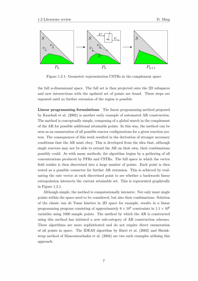
Figure 1.2.1: Geometric representation CSTRs in the complement space
the full n-dimensional space. The full set is then projected onto the 2D subspacesand new intersections with the updated set of points are found. These steps arerepeated until no further extension of the region is possible.
Linear programming formulations The linear programming method proposedby Kauchali et al. (2002) is another early example of automated AR construction.The method is conceptually simple, composing of a global search in the complementof the AR for possible additional attainable points. In this way, the method can beseen as an enumeration of all possible reactor configurations for a given reaction sys-tem. The consequences of this work resulted in the derivation of stronger necessaryconditions that the AR must obey. This is developed from the idea that, althoughsingle reactors may not be able to extend the AR on their own, their combinationspossibly could. As with many methods, the algorithm begins by a gathering of allconcentrations produced by PFRs and CSTRs. The full space in which the vectorfield resides is then discretised into a large number of points. Each point is thentested as a possible connector for further AR extension. This is achieved by eval-uating the rate vector at each discretised point to see whether a backwards linearextrapolation intersects the current attainable set. This is represented graphicallyin Figure 1.2.1.
Although simple, the method is computationally intensive. Not only must singlepoints within the space need to be considered, but also their combinations. Solutionof the classic van de Vusse kinetics in 2D space for example, results in a linearprogramming program consisting of approximately 6× 10³ constraints in 1.1× 10⁶
variables using 1000 sample points. The method by which the AR is constructedusing this method has initiated a new sub-category of AR construction schemes.These algorithms are more sophisticated and do not require direct enumerationof all points in space. The IDEAS algorithm by Burri et al. (2002) and Shrink-wrap method of Manousiouthakis et al. (2004) are two such examples utilising thisapproach.
7
1.2 Literature review D. Ming
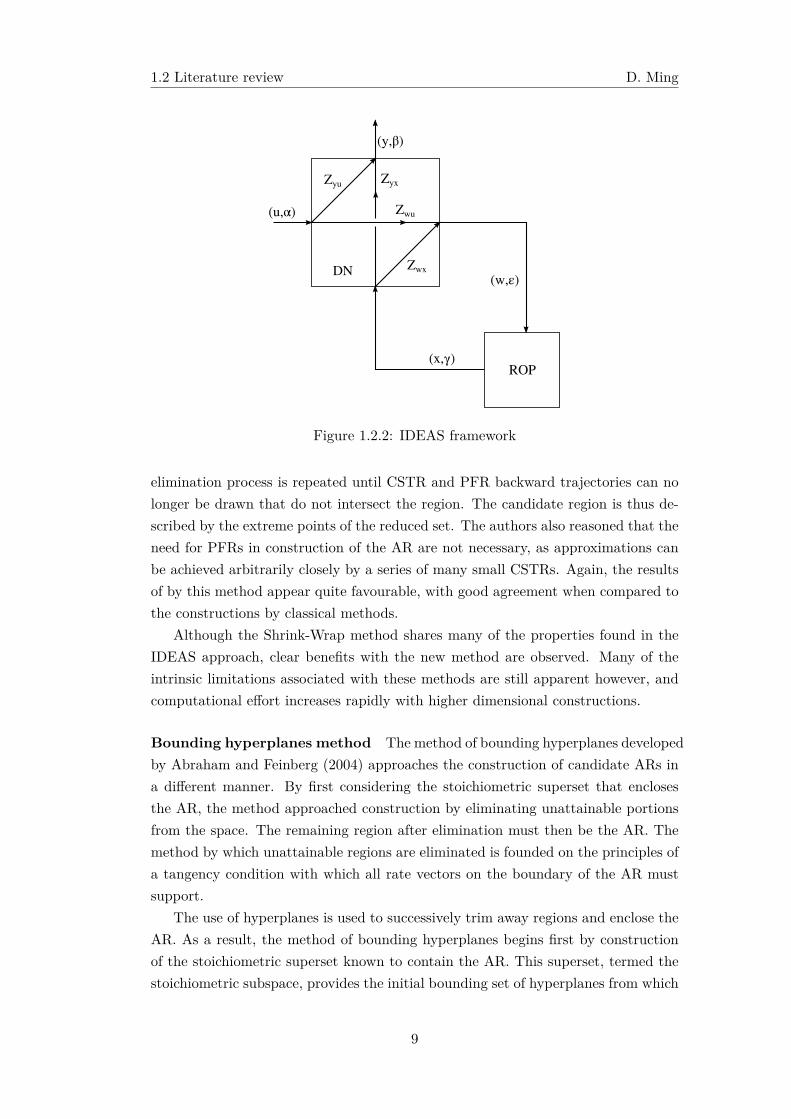
IDEAS and Shrink-wrap methods The Infinite DimEnsionAl State-space ap-proach (IDEAS) considers the problem of AR construction by solution of an infinitedimensional linear optimisation problem. Reactor networks are represented as thecombination of two blocks, shown in Figure 1.2.2. The first, termed the reactoroperator (ROP), aims to describe all actions undertaken by all reactors on processstreams. The second block, referred to as the distribution network (DN), is rep-resentative of all actions undertaken by mixing, splitting, recycling and bypassingof process streams. The ROP and DN are linked together by a number of streamsconnecting the inlets and outlets of each block to each other as well as to themselves.This network is used as the generalised representation of an arbitrary reactor sys-tem. Both the ROP and DN blocks produce linear constraints,. These form thebasis of a large linear optimisation procedure.
Construction of the AR occurs by solution of an infinite dimensional linear pro-gramming problem. Since, the solution of this kind of problem cannot be solvedanalytically, the authors propose an approximate solution by replacing the infin-ite dimensional problem with the solution of a series of finite dimensional linearproblems of increasing size. It is shown that the solution of the finite problem isguaranteed to converge to the infinite dimensional case and hence this provides ameans of AR construction. The results of the finite dimensional case approximatethe AR arbitrarily closely. The authors were able to construct 2D ARs for the wellunderstood van de Vusse kinetics using a number of finite approximations. Althoughmany simple lower dimensional constructions were achievable, the IDEAS algorithmsuffered from many of the challenges associated with point-sampling (linear program-ming) methods. A large number of number of constraints require consideration. Thisnumber increases rapidly for higher dimensional problems. Even under these cir-cumstances however, the IDEAS formulation is a generalised and flexible frameworkthat can be used to formulate and solve many other reactor synthesis problems thatare not related to the AR.
Based on the IDEAS framework, Manousiouthakis et al. (2004) proposed a num-ber of feasibility properties that reactor networks must obey. The properties wereemployed as a basis for the development of a new AR construction algorithm knownas the Shrink-Wrap method. Using these ideas, the authors proposed both a ne-cessary and sufficient condition for feasible concentrations founded on their formu-lations of new terms. These terms are referred to as inactive, active and isolatedsub-networks. The Shrink-Wrap method begins by constructing a convex supersetthat is known to contain the AR. The superset is then discretised into a number offinite points. From these points, extreme points of the superset are determined byway of a convex hull algorithm. The extreme points are used as generating pointsfrom which CSTR and PFR backward trajectories can be drawn. The superset is re-duced if a backward trajectory is found that does not intersect the current polytope.In this way, the method acts to trim away unachievable regions from the set. The
8
1.2 Literature review D. Ming
ROP
DN
Zyu Zyx
Zwu
Zwx
(u,α)
(y,β)
(x,γ)
(w,ε)
Figure 1.2.2: IDEAS framework
elimination process is repeated until CSTR and PFR backward trajectories can nolonger be drawn that do not intersect the region. The candidate region is thus de-scribed by the extreme points of the reduced set. The authors also reasoned that theneed for PFRs in construction of the AR are not necessary, as approximations canbe achieved arbitrarily closely by a series of many small CSTRs. Again, the resultsof by this method appear quite favourable, with good agreement when compared tothe constructions by classical methods.
Although the Shrink-Wrap method shares many of the properties found in theIDEAS approach, clear benefits with the new method are observed. Many of theintrinsic limitations associated with these methods are still apparent however, andcomputational effort increases rapidly with higher dimensional constructions.
Bounding hyperplanes method The method of bounding hyperplanes developedby Abraham and Feinberg (2004) approaches the construction of candidate ARs ina different manner. By first considering the stoichiometric superset that enclosesthe AR, the method approached construction by eliminating unattainable portionsfrom the space. The remaining region after elimination must then be the AR. Themethod by which unattainable regions are eliminated is founded on the principles ofa tangency condition with which all rate vectors on the boundary of the AR mustsupport.
The use of hyperplanes is used to successively trim away regions and enclose theAR. As a result, the method of bounding hyperplanes begins first by constructionof the stoichiometric superset known to contain the AR. This superset, termed thestoichiometric subspace, provides the initial bounding set of hyperplanes from which
9
1.2 Literature review D. Ming
additional bounding hyperplanes can be introduced. Corners of the polytope arecalculated and used as starting points for the trimming process. At each corner ofthe current polytope, a new hyperplane is introduced. Its orientation is calculatedfrom the orientation of the other hyperplanes which contribute to the corner andcan be thought of as an average orientation of the hyperplanes passing through thecorner point. The hyperplane is then moved into the current polytope until either atangency point is found, or the feed vector is excluded. The hyperplane is then addedto the set of bounding planes, and the corners the new polytope are determined.This process is repeated until no additional hyperplane can be added to trim awaya region. The resulting region is then generally a fairly accurate approximation tothe AR.
The bounding hyperplanes method is fairly robust but is computationally ex-pensive to perform. The method has shown to be particularly effective in handlingkinetics that involve multiple steady states. Construction occurs as an eliminationof infeasible regions, rather than an addition of potentially feasible points. Themethod does not appear to scale very well with increasing dimension. A comparisonof construction times for the van de Vusse problem in 2D and 3D shows that the3D problem may take up to ten times longer to complete (Abraham, 2005). As aresult, construction accuracy may suffer if higher dimensional problems are to beaccomplished in reasonable time. These issues are in part due to the extra com-putational workload associated with the calculation of the corners in the currentpolytope (vertex enumeration).
Recursive constant control policy method The recursive constant control(RCC) policy algorithm developed by Seodigeng et al. (2009) is one of the mostrecent contributions to the field of AR construction algorithms. By exploiting thedual nature of the DSR equation and with knowledge that DSRs provide final accessto the boundary of the AR (Feinberg, 2000b), candidate ARs may be constructedfairly easily in an iterative manner by use of a single reactor equation. The algorithmis particularly fast. Unlike the other methods discussed, the RCC algorithm does notappear to suffer from higher dimensional constructions in the way that discretisation-type algorithms do. This may be due to fact that the algorithm does not attempt toperform a search over the entire region. However, since the method only performs alocal search, method generally does not produce the correct result for kinetics withmultiple steady states. The method of construction is simple. Construction beginswith the integration of the DSR equation from the feed for multiple values of thecontrol policy parameter α. Here the value of α is fixed for a given integration andtakes on values between 0 and ∞. For the range of α values chosen, a family of DSRtrajectories are produced. Feed and equilibrium points are chosen as mixing pointsin the DSR equation. The convex hull of the points from this family is determinedand this constitutes the first candidate AR approximation. The second stage of the
10
1.2 Literature review D. Ming
algorithm utilises the extreme points of the convex hull as generating points for newDSR trajectories. For each extreme point, the above procedure is repeated, with arange of constant α values chosen and their respective trajectories calculated. Thepoints belonging to these new trajectories are then combined with the existing setof extreme points and the convex hull of the new set of points is found. The thirdstage further populates the region with additional DSR trajectories belonging to α
values chosen to increase the number of α values in the specified range of α values.This procedure is repeated until no further growth is achieved. The convex hullresulting from this serves to represent the AR candidate.
1.2.2 Batch optimisation
Batch reactors and batch operation are common in many industries where highvalue, low volume products are produced. Batch reaction is also often consideredto be more versatile than continuous operation, and lends itself well to small-scalework, such as that developed in experimental and piloting operations. The useof batch and semi-batch reactors thus forms an important part in the processingof many specialist chemicals, pharmaceuticals, and food-related products. For thisreason, significant effort has been undertaken over the years towards the appropriatesynthesis (Allgor et al., 1996; Zhang and Smith, 2004), optimisation (Levien, 1992;Vassiliadis et al., 1994) and understanding (Brooks, 1988; Bonvin, 1998; Luus andOkongwu, 1999; Puigjaner, 1999; Yi and Reklaitis, 2006) of batch processes.
It follows that a large amount of research on batch optimisation and reactionalready exists, and the scope of work in this area is vast. In general, two broad areasof batch optimisation exist:
1. Batch unit optimisation, in which batch unit operations are investigated andimproved. Batch reactor optimisation is accordingly a subset of this.
2. Batch process optimisation, in which interactions between different processingstages are analysed and improved. The entire batch plant is optimised as awhole.
The first category is concerned with the optimisation of individual batch units. Thisoften leads to the development of kinetic and transfer models with respect to timethat are then optimised, often in isolation, to the remainder of the batch plant. Theoptimisation of batch reactors necessarily falls within this category, although interestin this specific field is understandably still vast, due to the importance of batchreaction as a whole. Issues such as component production and yield maximisationare often areas of interest within this scope.
In contrast, batch process optimisation deals with optimisation of the entirebatch plant. This includes not only the selection and integration of all batch unitswithin the plant (mixing, reaction and separation unit operations), but also factors
11
1.2 Literature review D. Ming
related to the transfer and timing of material throughout the plant within the pro-duction campaign must be considered. Since batch equipment is far more versatilethan continuous equipment, the appropriate and optimal use of batch equipment isoften far more challenging, resulting a much more complex problem than the op-timisation of a single batch unit operation. This requires the spatial arrangementof batch equipment on the plant floor, as well as the organisation and schedulingof batch equipment in time. Issues such as changeovers resulting from multipleproducts, trade-offs from multiple objectives, product order changes and demandpatterns, minimising makespan (the total time for all jobs to complete), optimalallocation of resources, changeovers, inventory sizes, sanitisation, shelf-life etc. arereadily encountered in a multi-product batch plants. Honkomp et al. (2000) discusshow even when mathematically sound scheduling models have been developed, thescheduler may still invest a large amount of time adjusting the model to accountfor unexpected details that spoil the production plan. Batch process synthesis (thedesign of batch process), may also fall within the scope of this field. Indeed, the spanof batch process research is vast, covering many fields of expertise under a singlebranch.
Furthermore, the advancement of computer technology has allowed for a greatersurge of interest in batch optimisation, where easily accessible computational powercan be paired with numerical non-linear optimisation techniques. To this end, suchtechniques often employ traditional optimisation and optimal control methods, andare common in reactor design and modelling. Similar to that discussed in section1.1, these works tend to focus on the optimisation of a problem given a specificmodel, but do not always exploit structure in a system, an approach that the ARexcels in. A cursory overview of the efforts made to batch improvement is givenbelow.
Batch process scheduling and optimisation
For the optimisation of batch processes, scheduling is fundamental to the adequateoperation of the plant by optimal allocation of a fixed number of resources, over aset time from a potentially a number of desired products from a batch recipe. Differ-ent products may then be produced on common pieces of equipment, with sharingof intermediate products. Batch plants are generally classifiable into two funda-mental types, based on the nature of production within the facility: multiproduct(or flow-show) problems are those belonging a production facility where all productsundergo the same set of tasks in the same order (such as a conventional productionline). All products must undertake the same path through the production line. Themultipurpose (job-shop) representation is a generalisation of flow-shop scheduling.Here, different jobs require a different order of tasks, and so each job may undergoa different sequence within the plant. Orders may even visit the same task multiple
12
1.2 Literature review D. Ming
times(Li and Ierapetritou, 2008). The path of each product is then different to otherpaths for other products.
The representation of time is important in batch scheduling, as often objectivefunctions for the plant optimisations are formulated around issues often related tomakespan, tardiness, earliness, etc. The modelling of batch schedules is handled bytwo common approaches in time. Discrete time modelling of batches is the class ofproblems that attempt to divide the scheduling horizon into a discrete number oftime intervals of fixed size. Tasks are then initiated and completed only at discretepoints defined by the boundaries of the discretised time intervals. This simplifies thecomplexity of the resulting model, as only a discrete number of points and variablesare considered, although this also limits the possible solution set and may also resultin degenerate or infeasible solutions depending on the grid size. The accuracy andquality of solution is then strongly correlated to the number of time intervals chosenfor the scheduling horizon. A further drawback of discrete time modelling is thatthe resulting model is typically large, encompassing a large number of variablesassociated with each discrete time interval. This limits the application of discretetime formulations to realistic problems. Continuous time representations aim tomitigate these issues by allowing timing decisions in the corresponding model tooccur over a continuous time range. Decisions are then modelled as continuousvariables indicating the exact time when tasks are completed or initiated. Typically,this results in more complex model formulations resulting from more sophisticatedresource constraints(Mendez et al., 2006).
Similarly, the representation of material flows in the batch plant is handled bytwo common models. Network flow equations often either follow State Task Network(STN) or Resource Task Network (RTN) approaches. In STN based models, thebatch plant is assumed to consume or produce materials (states) at processing nodes.The plant is then represented as a directed graph containing two distinct node types:state nodes (feed, intermediate and final products), task nodes (process operationsthat transform feed material into one or more output state), and arcs connectingstate nodes to task nodes. This representation fits closely to that of a conventionalprocess flow diagram. In RTN based models, the batch plant is represented as aset of nodes in which both material and processing resources such as storage arecarried by the node. That is, nodes not only represent material and equipment, butalso utility resources such as heating and storage. Processing and storage tasks areassumed to consume and release resources at their starting and ending times(Mendezet al., 2006). Pinto et al. (2008) provides a detailed analysis between the relativestrengths of STN and RTN based models.
Furthermore, batch schedules can be distinguished based on their usage cases.Two modes are identified. Online applications refer to those that are used frequentlyto guide process operations over a constantly changing horizon time. In this way,online schedules are similar to plant controller problems (Honkomp et al., 2000). By
13
1.2 Literature review D. Ming
comparison, offline applications are used to make process decisions in a simulationenvironment in which several scenarios can be investigated and used to guide theactions of the management team.
Capon-Garcia et al. (2011) provide a complex mathematical batch schedulingmodel involving both economic and environmental constraints including, but notlimited to, equipment changeover environmental interventions, raw material andproduct manufacturing environmental interventions. This leads to a multi-objectiveMINLP problem that provides a range of feasible solutions depending on the decisionmaker’s criteria. Environmental assessments are mathematically formulated by useof Life Cycle Inventories (LCI), which are directly associated with the product andchangeover recipes of the plant. A case study involving the manufacture of acrylicfibres in a multi-product batch plant is provided.
The area of dynamic scheduling (schedules that may be adjusted in real-time)has attracted the attention of of many batch researchers due to its practical focus onproduction. Scheduling of this type is often also referred to as reactive scheduling.Novas and Henning (2010) discuss a scheduling methodology for repair-based events.Cott and Macchietto (1989) introduce the idea of a real-time controller that measuresdeviations from the schedule and then forecasts the potential delays in production.Starting times for subsequent batches are then modified to minimise disruptions.Kanakamedala et al. (1994) provide a similar treatment to multipurpose batch plantsbased on a look-ahead heuristic that chooses alternatives which minimise impact tothe rest of the schedule. Since it is a heuristic method, computation complexity maybe reduced, however a completely theoretical approach may provide better solutions.A review of common reactive scheduling techniques is also discussed in (Ouelhadjand Petrovic, 2009).
Indeed, scheduling operations are broad enough to include many aspects ofscheduling. These ideas may be transferred to related fields in operations research.For instance, Shah (2004) provides a general treatment for scheduling to the phar-maceuticals industry specific for supply chain modelling. The author provides anoverview of challenges faced as well as describes how scheduling theory can be formu-lated and applied. Many of the ideas discussed in the work relate to the continuoustime modelling scheduling problems utilised in batch plant scheduling models.
Similarly, Grossmann (2005) details the use of scheduling techniques to an emer-ging field of operations research termed enterprise-wide optimisation (EWO), inwhich optimisation of not only the plant, but more generally the entire supplychain, such as the operations of supply and distribution are included in the for-mulation. The author describes key challenges, such as the adequate formulationof non-linear mathematical models that describe the entire supply chain includinguncertainties, the solution of these models, and the eventual implementation of theproposed solutions over a large time horizon (potentially involving many years).EWO is a new field where existing scheduling techniques and expertise may be ex-
14
1.2 Literature review D. Ming
panded into related and enterprise-centric interest areas. Wassick (2009) provides arelated discussion to EWO, whereas Biegler and Zavala (2009); Grossmann (2012)propose a number of possible solution methods theories suitable for EWO prob-lems. Varma et al. (2007) provide an interesting and extensive discussion on EWOaspects, incorporating strategic and tactical R&D management decisions into themodel formulation. The authors highlight mathematical strategic and tactical en-terprise models, and discuss a generalised enterprise wide network model consistingof planning and process functions. The integration of financial and operational de-cision models is also considered.
Li and Ierapetritou (2008) review a number of strategies for the mathematicalformulation of uncertainties in the batch schedule. Whereas a number of traditionalscheduling approaches adopt the view of deterministic models for their optimisation,the authors indicate how uncertainties in scheduling present different problems withtheir own solution strategies. Within this work, the authors describe how problemssuch as demand changes (rush orders), unexpected breakdowns, processing and re-cipe variability, and price changes might be handled. The work details how thismay achieved via three distinct representations of uncertainty: placing bounds onthe uncertain variables, probability distributions and fuzzy representations. Eachof these is associated with a specific solution technique, although all methods oftenassume the form of a complex MILP or MINLP problem after reformulation.
Although scheduling problems are often solved in well developed commercialoptimisation software (GAMS, AMPL, etc.), Wang et al. (1996); Chunfeng and Xin(2002); Ponsich et al. (2008a,b); Liu et al. (2010) describe various alternate methodsfor determining optimal batch schedules via a number of evolutionary algorithmsincluding genetic algorithms and particle swarm optimisation.
The complexity of batch scheduling has attracted the attention of many aca-demics over the years. Several batch process literature reviews have been producedas a result. Mendez et al. (2006) is considered the most recent contribution on thesubject, discussing the issue of short-term scheduling problems in batch plants. Thework provides a thorough treatment of dominant mathematical equations used todescribe sequential batch and batch network plants. The authors categorise thebreadth of batch scheduling problems, and discusses their solution by two workedcase studies. Notably, the authors describe how scheduling problems may be for-mulated in different ways (through time and event representation, material balancesand objective function formulations) which may make solution easier or more diffi-cult depending on the representation adopted. Two real-world examples are givendemonstrating the challenges faced by batch processes. The authors also provide alist of commercial and academic software used for short-term batch scheduling. Flou-das and Lin (2004) provide an extensive comparison between continuous-time anddiscrete-time formulations in batch scheduling. The authors highlight the strengthsand weaknesses of each approach, and also provide common mathematical formula-
15
1.2 Literature review D. Ming
tions for describing generalised batch schedules with each approach. Performancecomparisons between the two are also briefly highlighted, and topics related to react-ive scheduling and uncertainty are also briefly discussed. Kallrath (2002); Reklaitis(1996); Shah (1998) all provide many other excellent reviews related to aspects ofbatch scheduling and modellilng.
Batch reactor optimisation
Graphical methods Batch optimisation using graphical methods, particularlywith regard to the problem of efficient waste-water allocation are already known.Notable contributions include (Wang and Smith, 1995b,a; Dhole et al., 1996; Hallale,2002; El-Halwagi et al., 2003; Manan et al., 2004; Majozi et al., 2006; Chen and Lee,2008) in which many include formulations are based upon mass transfer operations.Hallale (2002) utilises a graphical approach similar to pinch analysis in heat ex-changer network synthesis for the minimisation of water in what is referred to theauthor as a surplus water diagram. A graphical optimisation based on dynamic pro-gramming has also been investigated by Staniskis and Levisauskas (1983), whereasseveral analyses using graphical methods to fermentation processes are discussed byShioya and Dunn (1979).
O’Reilly (2002) considers a batch reactor operating under the hypothetical re-action scheme I + R → A + 2D and A + R → IMPS in which A and D are saleableproducts and IMPS is a waste product. The formulation includes a detailed un-steady state mass and energy balance including aspects of mixing efficiency in theform of impeller speed, as well as heat transfer efficiency from fouling. Notably,the author describes a short-cut method for producing the results when detailedkinetic data for the reaction is not available. This is achieved using thermochemicaldata and a yield profile with respect to time. Solution trajectories and temperatureprofiles are generated using Microsoft Excel.
Optimal control theory and Pontryagin’s maximum principle The ap-plication of Pontryagin’s maximum principle to batch optimisation is commonlyfound in literature. Use of the technique, specifically to optimal batch operationin fermentation processes, has been performed by Modak et al. (1986); Modak andLim (1989, 1992). In particular, the authors investigated general characteristicsof feeding rate profiles for fed-batch operation, and later expanded the theory fortwo control variables (Modak et al., 1986; Modak and Lim, 1989). The problem ofmaximising metabolite yield and productivity in these systems was also later ex-plored by Modak and Lim (1992). Similarly, Srinivasan and Bonvin (2003) usedthe maximum principle to identify conditions for optimal feed rate and temperaturepolicies for systems of batch and fed-batch reactors with two reactions. The authorsconclude that it may be difficult to find a general analytic theory for systems in-volving more than two reactions. Filippi-Bossy et al. (1989) considered the use of
16
1.2 Literature review D. Ming
tendency models to batch reactor optimisation. The method involved the joint useof experimental data and a suggested dynamic model to systematically improve theproposed model estimate with each successive experimental run. The authors usedPontryagin’s maximum principle to calculate optimal trajectories that were usedto anticipate the optimal trajectory of the next run. However, the authors notedthat a priori knowledge of the reaction order was necessary, and that the success ofthe method relied on the accuracy of the base model. Uhlemann et al. (1994) alsoconsidered the use of tendency models and suggested that optimisation of fed-batchreactors be viewed as a two-step process first involving the determination of off-linecontrol variables followed by an optimal control phase. Although the applicationof Pontryagin’s maximum principle is popular in batch optimisation, the determin-ation of optimal solutions with the technique is difficult, particularly if analyticalsolutions are required. Shukla and Pushpavanam (1998) observe that this may beas a result of numerical instability and a priori knowledge of the sequence of controlactions for adequate convergence.
Non-linear programming methods Optimisation of batch processes by dy-namic optimisation has been investigated by Dhir et al. (2000); Aziz and Mujtaba(2002). Conversion of the problem and solution via non-linear programming meth-ods are also common (Garcia et al., 1995; Allgor and Barton, 1997), with broaderformulations to include separation processes for example (Allgor and Barton, 1999).Cuthrell and Biegler (1989) used sequential quadratic programming to obtain op-timal operating policies in fed-batch reactors involving discontinuous profiles. Push-pavanam et al. (1999) applied the same approach for determining optimal feedingprofile, also in fermentation processes.
The use of non-linear programming methods are discussed by Allgor et al. (1999)and Allgor and Barton (1999). Cuthrell and Biegler (1989) used sequential quadraticprogramming to obtain optimal operating policies in fed-batch reactors involvingdiscontinuous profiles. Pushpavanam et al. (1999) applied the same approach fordetermining optimal feeding profile in fermentation processes. Garcia et al. (1995)demonstrated how the optimisation of batch reactors could be achieved by convertingan optimal control problem into an equivalent non-linear programming problem. Thesolution is then found by a generalised reduced gradient approach and a golden searchmethod for determination of the optimal final time. The practical implementationof optimal feeding profiles in fed-batch reactors is also considered by Shukla andPushpavanam (1998). The authors approximated optimal profiles using discretepulses and constant flow rates over both equal and unequal sub-intervals.
The optimisation of batch processes by dynamic optimisation has been invest-igated by Allgor et al. (1999); Dhir et al. (2000); Aziz and Mujtaba (2002). Peterset al. (2006) considered the design of an online controller for the optimal control ofbatch reactors using dynamic optimisation. In this way, changes in plant dynamics
17
1.3 Motivation D. Ming
are adjusted to provide an optimal control loop without the need for offline analysis.
Stochastic optimisation methods Recently, the successful use of stochasticmethods to batch optimisation has also been investigated. In particular, the useof genetic algorithms for the determination of optimal feeding profile have beeninvestigated by Ronen et al. (2002); Sarkar and Modak (2003); Zuo and Wu (2000).Zuo and Wu (2000) in particular modelled the cultivation of biological productswith hybrid neural networks and then optimised the production rate using geneticalgorithms. Faber et al. (2005) utilised a simulated annealing technique to improvethe convergence of dynamic optimisation methods. The method was applied tothe maximisation of intermediate species concentrations. Zhang and Smith (2004)considered the determination of optimal, non-ideal batch and fed-batch systemsvia a superstructure approach; optimal optimisation parameters were then solvedalso using simulated annealing. In addition to determining optimal control policies,the statistical nature of stochastic methods also allows for the discovery of similarnear-optimal control policies. Slow convergence may still be an issue with thesealgorithms however.
1.3 Motivation
1.3.1 AR construction algorithms
In section 1.2.1, we indicated how recent developments in AR theory have tended tofocus on formulating efficient and accurate methods for numerical AR construction.The existence of these methods are important, mainly for two reasons: firstly forthe advancement of fundamental AR theory, and secondly for the application thesemethods to modern problems.
Despite there being a large body of work on AR theory, an adequate sufficiencycondition for the AR still does not exist. The application of AR theory to manyproblems is still subject to uncertainty. It is still not well understood whether a givenregion is the true AR, or only a subset of it. AR constructions are still referred toas candidate attainable regions as a result.
Furthermore, development of efficient AR construction methods is required be-cause current approaches are still computationally strenuous for modern problemsof interest. Constructions in four dimensions and higher are cumbersome to viewand work with, and so graphical techniques are either slow or not well suited forthis purpose. In this regard, the often termed ‘curse of dimensionality’ by Bellman(2010) is appropriate for AR construction schemes. Current methods often rely ona discretisation of concentration space followed by either a direct search or somevariant on traditional optimisation. The successful development of faster, more ef-ficient methods, and a better understanding of the challenges involved would allow
18
1.3 Motivation D. Ming
for more confidence in the recommendations suggested by AR algorithms.AR construction methods therefore are necessary, not only because of the com-
plexity of higher dimensional problems, but also because they facilitate developmentof conventional AR theory towards a sufficiency condition.
1.3.2 Batch reactors
Similarly, there also exists a need for improved techniques in batch reactor synthesisproblems. Irrespective of the specific numerical technique employed, the underlyingmethodology to batch improvement of current methods is generally consistent. Amathematical model describing the system is formulated and then solved by ad-justing operating parameters, such as feed addition rate and temperature, until anassigned performance index is optimised. Optimisation is thus carried out by de-termination of an optimal combination of parameters for a fixed method of batchoperation. The solution to the problem is then resultant from a mathematical formu-lation of a non-linear optimisation problem. The success and quality of the solutionis often also dependent on an initial guess, which, may be linked to one of manylocal optima. In order for convergence to the true global optimum to be established,one must choose a starting guess that is sufficiently close to the answer. This iscommon to both batch and continuous optimisation problems. Specific examplesof this to reactor synthesis arise when mixtures are introduced (McGregor et al.,1999; Godorr et al., 1999). Certain objective functions may be difficult to formulatemathematically given particular time and event representations, which may lead toadditional auxiliary variables and complex constraints that ultimately influences thesolution and solution performance.
Often, fed-batch reactors are utilised specifically in batch reactor optimisation,as this allow for flexibility in the problem types and optimisation routines employed.Little is currently found in the scientific literature detailing how other reactor typesmight be employed for the improvement of batch reactors, or even how combinationsof different reactors may be arranged together to form a complex structure thatachieves the desired task. This aspect of batch reactors specifically is still missingin the field.
In this regard, further improvements might be realised by also considering batchstructure, in a similar manner to that achieved in continuous reactors. By batchstructure, we mean the specific selection and sequencing of batch reactive equip-ment that produces a particular output state. Once the appropriate structure isestablished, optimisations may be carried out in the usual manner, offering furtherimprovement to the problem. Following from arguments related to the continuouscase, the first goal in batch optimisation should be to arrive at the correct reactorstructure before optimisations are performed. With this in mind, use of the ARapproach to batch reactors could be helpful in providing a better understanding of
19
1.4 Conclusion and scope of work D. Ming
optimal batch reaction sequence.Even as the benefits of AR theory have been clearly demonstrated with con-
tinuous reactors, the method has seen little adoption in a batch setting. In almost40 years since its initial development, only a single paper on the application of ARtheory in batch reactors (Davis et al., 2008) exists excluding this work. This is duein large part to the fact that AR theory has historically developed with continuousreaction in mind.
1.4 Conclusion and scope of this work
Earlier in section 1.2.2, we discussed how the field of batch optimisation may becategorised into two broad fields: batch unit optimisation, and batch process optim-isation. In this work we will be specifically focussed on the reactive portion of batchprocesses. That is, although the breadth of batch optimisation problems is vast,encompassing many different operations and scheduling problems, the particularbenefit offered by AR theory necessitates that improvements to batch processes arefocussed specifically on batch reactors, and not on the entire batch plant. With thebackground of improvement through structure discussed, and motivation of thesedetailed above, this thesis aims to address two areas in AR and batch reactor theory:
1. To continue the development of robust AR construction methods: providing adeeper insight into the challenges and potential improvements of these meth-ods.
2. Towards the improvement of batch reactors via structure: utilising the in-sights gained from AR theory and applying them to batch operations. In laterchapters, it will be our specific aim to exploit the benefits of continuous ARresults, and apply it directly to equivalent batch systems.
The AR is a powerful method that has seen little adoption other than to prob-lems mainly posed in R2 and R3 with continuous processes in mind. Although itis currently possible to address non-adiabatic systems, unbounded constructions,comminution and basic separation operations, little work has been attempted to ap-proach related problems in batch reactors. Most of these methods are also held backby slow construction times or limited to lower dimensions. The use of the methodto a wider audience may help to spread its use to broader fields, but it is our viewthat the above two points limit adoption of AR methods and ideas as a generallyaccepted, and easily accessible theory. Further research into this theory is requiredin order to make it more accessible. This should be done rather with an emphasison graphical meaning as opposed to mathematical rigour. It is the goal of this thesisto help close these two gaps. In this way, this thesis essentially communicates theideas of alternative methods to traditional process optimisation. The emphasis inthis work will be towards reactor structure, rather than on optimisation alone.
20
References D. Ming
In order for this to be done, the reader should first be familiar with basic ARtheory. This can be found in chapter 2, where a brief overview of the AR is discussed.From there, the benefit in exploiting reactor structure should be more apparentas a means for improvement, so that the same way of thinking can be appliedto batch reactors. This is partly achieved in chapter 3, where improvements instructure ultimately bring about an improvement in production rate. In chapter4, improvements to an existing outside-in AR construction algorithm are discussed.The direct application of AR theory to batch reactors is given treatment in chapter5. Final conclusions and recommendations for future research are then made inchapter 6. Where appropriate, specific theory and definitions have been split intothe relevant chapters and used when necessary so that the reader is not required toread this work in a linear fashion.
1.5 Copyright permissions
The majority of this work has been formed from the compilation of published work(chapters 3, 4 and 5 respectively). Copyright permissions have been granted by thepublishers for these chapters as a result. The content in these chapters has beenadapted for use in this thesis from their respective papers given below.
• Chapter 3: Ming, D., Hildebrandt, D., Glasser, D., 2012. A Graphical Methodof Improving the Production Rate from Batch Reactors. Ind. Eng. Chem.Res. 51, 13562–13573.
• Chapter 4: Ming, D., Hildebrandt, D., Glasser, D., 2010. A revised methodof attainable region construction utilizing rotated bounding hyperplanes. Ind.Eng. Chem. Res. 49, 10549–10557.
• Chapter 5: Ming, D., Glasser, D., Hildebrandt, D., 2013. Application ofAttainable Region theory to batch reactors. Chem. Eng. Sci. 99, 203 – 214.
References
Abraham, T. K., 2005. Kinetic bounds on attainability in the reactor synthesisproblem. Ph.D. thesis, Ohio State University, Ohio.
Abraham, T. K., Feinberg, M., 2004. Kinetic bounds on attainability in the reactorsynthesis problem. Industrial & Engineering Chemistry Research 43 (2), 449–457.
Agarwal, V., Thotla, S., Mahajani, S. M., 2008. Attainable regions of reactivedistillation-part i. single reactant non-azeotropic systems. Chemical EngineeringScience 63 (11), 2946–2965.
Allgor, R. J., Barrera, M. D., Barton, P. I., Evans, L. B., 1996. Optimal batchprocess development. Computers & Chemical Engineering 20 (6-7), 885–896.
21
References D. Ming
Allgor, R. J., Barton, P. I., 1997. Mixed-integer dynamic optimization. Computers& Chemical Engineering 21, Supplement (0), S451–S456.
Allgor, R. J., Barton, P. I., 9 1999. Screening models for batch process development:Part ii. case studies. Chemical Engineering Science 54 (18), 4065–4087.
Allgor, R. J., Evans, L. B., Barton, P. I., 10 1999. Screening models for batch processdevelopment: Part i. design targets for reaction/distillation networks. ChemicalEngineering Science 54 (19), 4145–4164.
Aziz, N., Mujtaba, I. M., 1 2002. Optimal operation policies in batch reactors.Chemical Engineering Journal 85 (2-3), 313–325.
Bellman, R., July 2010. Dynamic Programming. Princeton Landmarks in Mathem-atics. Princeton University Press.
Biegler, L. T., Zavala, V. M., 2009. Large-scale nonlinear programming using ipopt:An integrating framework for enterprise-wide dynamic optimization. Computers& Chemical Engineering 33 (3), 575–582.
Bonvin, D., 1998. Optimal operation of batch reactors - a personal view. Journal ofProcess Control 8 (5-6), 355–368.
Brooks, B. W., 1988. Semi-batch reactors and their use for autocatalytic reactions.Chemical Engineering Science 43 (6), 1287–1290.
Burri, J. F., Wilson, S. D., Manousiouthakis, V. I., 2002. Infinite dimensional state-space approach to reactor network synthesis: Application to attainable regionconstruction. Computers & Chemical Engineering 26 (6), 849–862.
Capon-Garcia, E., Bojarski, A. D., Espuna, A., Puigjaner, L., 2011. Multiobjectiveoptimization of multiproduct batch plants scheduling under environmental andeconomic concerns. AIChE Journal 57 (10), 2766–2782.
Chen, C., Lee, J., 7 2008. A graphical technique for the design of water-using net-works in batch processes. Chemical Engineering Science 63 (14), 3740–3754.
Chunfeng, W., Xin, Z., 2002. Ants foraging mechanism in the design of multiproductbatch chemical process. Industrial & Engineering Chemistry Research 41 (26),6678–6686.
Cornuejols, G., Tutuncu, R., January 2007. Optimization Methods in Finance(Mathematics, Finance and Risk). Cambridge University Press.
Cott, B., Macchietto, S., 1989. Minimizing the effects of batch process variabilityusing online schedule modification. Computers & Chemical Engineering 13 (1),105–113.
Cuthrell, J. E., Biegler, L. T., 1989. Simultaneous optimization and solution methodsfor batch reactor control profiles. Computers & Chemical Engineering 13 (1-2),49–62.
Davis, B. J., Taylor, L. A., Manousiouthakis, V. I., 2008. Identification of the at-tainable region for batch reactor networks. Industrial & Engineering ChemistryResearch 47 (10), 3388–3400.
22
References D. Ming
Dhir, S., Jr., K. J. M., Rhinehart, R. R., Wiesner, T., 2000. Dynamic optimizationof hybridoma growth in a fed-batch bioreactor. Biotechnology and bioengineering67 (2), 197–205.
Dhole, V. R., Ramchandani, N., Tainsh, R. A., Wasilewski, M., 1996. Make yourprocess water pay for itself. Chemical Engineering 103 (1), 100–103.
El-Halwagi, M., Gabriel, F., Harell, D., 2003. Rigorous graphical targeting for re-source conservation via material recycle/reuse networks. Industrial & EngineeringChemistry Research 42 (19), 4319–4328.
Faber, R., Jockenhovel, T., Tsatsaronis, G., 1 2005. Dynamic optimization withsimulated annealing. Computers & Chemical Engineering 29 (2), 273–290.
Feinberg, M., 1999. Recent results in optimal reactor synthesis via attainable regiontheory. Chemical Engineering Science 54 (13-14), 2535–2543.
Feinberg, M., 2000a. Optimal reactor design from a geometric viewpoint - iii. criticalcfstrs. Chemical Engineering Science 55 (17), 3553–3565.
Feinberg, M., 2000b. Optimal reactor design from a geometric viewpoint. part ii.critical sidestream reactors. Chemical Engineering Science 55 (13), 2455–2479.
Feinberg, M., Hildebrandt, D., 1997. Optimal reactor design from a geometricviewpoint- i. universal properties of the attainable region. Chemical EngineeringScience 52 (10), 1637–1665.
Filippi-Bossy, C., Bordet, J., Villermaux, J., Marchal-Brassely, S., Georgakis, C.,1989. Batch reactor optimization by use of tendency models. Computers & Chem-ical Engineering 13 (1-2), 35–47.
Floudas, C. A., Lin, X., 2004. Continuous-time versus discrete-time approaches forscheduling of chemical processes: a review. Computers & Chemical Engineering28 (11), 2109–2129.
Garcia, V., Cabassud, M., Lann, M. V. L., Pibouleau, L., Casamatta, G., 11 1995.Constrained optimization for fine chemical productions in batch reactors. TheChemical Engineering Journal and The Biochemical Engineering Journal 59 (3),229–241.
Glasser, D., Hildebrandt, D., 1997. Reactor and process synthesis. Computers &Chemical Engineering 21 (Supplement 1), S775–S783.
Glasser, D., Hildebrandt, D., Crowe, C., 1987. A geometric approach to steady flowreactors: The attainable region and optimization in concentration space. Industrial& Engineering Chemistry Research 26 (9), 1803–1810.
Godorr, S., Hildebrandt, D., Glasser, D., McGregor, C., 1999. Choosing optimalcontrol policies using the attainable region approach. Industrial & EngineeringChemistry Research 38 (3), 639–651.
Grass, D., Caulkins, J. P., Feichtinger, G., Tragler, G., Behrens, D. A., Septem-ber 2008. Optimal Control of Nonlinear Processes: With Applications in Drugs,Corruption, and Terror, 1st Edition. Springer.
23
References D. Ming
Grossmann, I., 2005. Enterprise-wide optimization: A new frontier in process sys-tems engineering. AIChE Journal 51 (7), 1846–1857.
Grossmann, I. E., 2012. Advances in mathematical programming models forenterprise-wide optimization. Computers & Chemical Engineering 47 (0), 2 – 18.
Hallale, N., 9 2002. A new graphical targeting method for water minimisation. Ad-vances in Environmental Research 6 (3), 377–390.
Hartmann, A. K., Rieger, H., September 2001. Optimization Algorithms in Physics,1st Edition. Wiley-VCH.
Hildebrandt, D., October 1989. The attainable region generated by reaction andmixing. Ph.D. thesis, University of the Witwatersrand, Johannesburg.
Hildebrandt, D., Glasser, D., Hausberger, B., Patel, B., Glasser, B. J., 2009. Pro-ducing transportation fuels with less work. Science 323 (5922), 1680–1681.
Honkomp, S., Lombardo, S., Rosen, O., Pekny, J., 2000. The curse of reality–whyprocess scheduling optimization problems are difficult in practice. Computers &Chemical Engineering 24 (2), 323–328.
Horn, F., 1964. Attainable and non-attainable regions in chemical reaction tech-nique. Pergamon Press, London.
Kallrath, J., 2002. Planning and scheduling in the process industry. OR spectrum24 (3), 219–250.
Kanakamedala, K. B., Reklaitis, G. V., Venkatasubramanian, V., 1994. Reactiveschedule modification in multipurpose batch chemical plants. Industrial & Engin-eering Chemistry Research 33 (1), 77–90.
Kauchali, S., Hausberger, B., Hildebrandt, D., Glasser, D., Biegler, L. T., 2004.Automating reactor network synthesis: Finding a candidate attainable region forthe water-gas shift (wgs) reaction. Computers & Chemical Engineering 28 (1-2),149–160.
Kauchali, S., Rooney, W. C., Biegler, L. T., Glasser, D., Hildebrandt, D., 2002.Linear programming formulations for attainable region analysis. Chemical Engin-eering Science 57 (11), 2015–2028.
Khumalo, N., Glasser, D., Hildebrandt, D., Hausberger, B., Kauchali, S., 2006. Theapplication of the attainable region analysis to comminution. Chemical Engineer-ing Science 61 (18), 5969–5980.
Levien, K. L., 5 1992. Maximizing the product distribution in batch reactors: reac-tions in parallel. Chemical Engineering Science 47 (7), 1751–1760.
Li, Z., Ierapetritou, M., 2008. Process scheduling under uncertainty: Review andchallenges. Computers & Chemical Engineering 32 (4), 715–727.
Liu, B., Wang, L., Liu, Y., Qian, B., Jin, Y.-H., 2010. An effective hybrid particleswarm optimization for batch scheduling of polypropylene processes. Computers& Chemical Engineering 34 (4), 518–528.
Luus, R., Okongwu, O. N., 8 1999. Towards practical optimal control of batchreactors. Chemical Engineering Journal 75 (1), 1–9.
24
References D. Ming
Majozi, T., Brouckaert, C. J., Buckley, C. A., 3 2006. A graphical technique forwastewater minimisation in batch processes. Journal of environmental manage-ment 78 (4), 317–329.
Manan, Z. A., Tan, Y. L., Foo, D. C. Y., 2004. Targeting the minimum water flowrate using water cascade analysis technique. AIChE Journal 50 (12), 3169–3183.
Manousiouthakis, V. I., Justanieah, A. M., Taylor, L. A., 2004. The shrink-wrapalgorithm for the construction of the attainable region: An application of theideas framework. Computers & Chemical Engineering 28 (9), 1563–1575.
Matlock, M. M., Howerton, B. S., Atwood, D. A., 11 2002. Chemical precipitationof heavy metals from acid mine drainage. Water research 36 (19), 4757–4764.
McGregor, C., Glasser, D., Hildebrandt, D., 1999. The attainable region and pontry-agin’s maximum principle. Industrial & Engineering Chemistry Research 38 (3),652–659.
Mendez, C. A., Cerda, J., Grossmann, I. E., Harjunkoski, I., Fahl, M., 2006. State-of-the-art review of optimization methods for short-term scheduling of batch pro-cesses. Computers & Chemical Engineering 30 (6-7), 913–946.
Metzger, M. J., Glasser, B. J., Patel, B., Fox, J., Sempuga, B. C., Hildebrandt, D.,Glasser, D., 2012. Liquid fuels from alternative carbon sources minimizing carbondioxide emissions. AIChE Journal.
Milne, A. D., July 2008. The application of the attainable region cocept to theoxidative dehydrogenation of n-butaes in inert porous membrane reactors. Ph.D.thesis, University of the Witwatersrand, Johannesburg.
Modak, J. M., Lim, H. C., 1989. Optimal operation of fed-batch bioreactors withtwo control variables. The Chemical Engineering Journal 42 (2), B15–B24.
Modak, J. M., Lim, H. C., 1992. Optimal mode of operation of bioreactor for fer-mentation processes. Chemical Engineering Science 47 (15-16), 3869–3884.
Modak, J. M., Lim, H. C., Tayeb, Y. J., 1986. General characteristics of optimalfeed rate profile for various fed-batch fermentation processes. Biotechnology andbioengineering 28 (9), 1396–1407.
Nisoli, A., Malone, M. F., Doherty, M. F., 1997. Attainable regions for reaction withseparation. AIChE Journal 43 (2), 374–386.
Novas, J. M., Henning, G. P., 2010. Reactive scheduling framework based on do-main knowledge and constraint programming. Computers & Chemical Engineering34 (12), 2129–2148.
O’Reilly, A. J., 9 2002. Batch reactor optimization, profitability vs waste minimiz-ation. Chemical engineering research & design 80 (6), 587–596.
Ouelhadj, D., Petrovic, S., 2009. A survey of dynamic scheduling in manufacturingsystems. Journal of Scheduling 12 (4), 417–431.
Peters, N., Guay, M., DeHaan, D., 2006. Real-time dynamic optimization of non-linear batch systems. Canadian Journal of Chemical Engineering 84 (3), 338–348.
25
References D. Ming
Pinto, T., Barbósa-Póvoa, A. P. F., Novais, A. Q., 2008. Design of multipurposebatch plants: A comparative analysis between the stn, m-stn, and rtn represent-ations and formulations. Industrial & Engineering Chemistry Research 47 (16),6025–6044.
Ponsich, A., Azzaro-Pantel, C., Domenech, S., Pibouleau, L., 2008a. Constrainthandling strategies in genetic algorithms application to optimal batch plant design.Chemical Engineering and Processing: Process Intensification 47 (3), 420–434.
Ponsich, A., Touche, I., Azzaro-Pantel, C., Domenech, S., Pibouleau, L., Daydé,M., et al., 2008b. A grid-based environment for multiparametric pse applications:batch plant design case study. In: VECPAR 2008: 8th International ConferenceHigh Performance Computing for Computational Science. Vol. 5336.
Puigjaner, L., 1999. Handling the increasing complexity of detailed batch processsimulation and optimisation. Computers & Chemical Engineering 23 (Supplement1), S929–S943.
Pushpavanam, S., Rao, S., Khan, I., 1999. Optimization of a biochemical fed-batchreactor using sequential quadratic programming. Industrial & Engineering Chem-istry Research 38 (5), 1998–2004.
Reklaitis, G. V., 1996. Overview of scheduling and planning of batch process oper-ations. In: Batch processing systems engineering. Springer, pp. 660–705.
Ronen, M., Shabtai, Y., Guterman, H., 2002. Optimization of feeding profile fora fed-batch bioreactor by an evolutionary algorithm. Journal of Biotechnology97 (3), 253–263.
Rooney, W. C., Hausberger, B. P., Biegler, L. T., Glasser, D., 2000. Convex at-tainable region projections for reactor network synthesis. Computers & ChemicalEngineering 24 (2-7), 225–229.
Sarkar, D., Modak, J. M., 2003. Optimisation of fed-batch bioreactors using geneticalgorithms. Chemical Engineering Science 58 (11), 2283–2296.
Scott, F., Conejeros, R., Aroca, G., et al., 2013. Attainable region analysis forcontinuous production of second generation bioethanol. Biotechnology for biofuels6 (1), 171.
Seodigeng, T., Hausberger, B., Hildebrandt, D., Glasser, D., 2009. Recursive con-stant control policy algorithm for attainable regions analysis. Computers & Chem-ical Engineering 33 (1), 309–320.
Seodigeng, T. G., January 2006. Numerical formulations for attainable region ana-lysis. Ph.D. thesis, University of the Witwatersrand, Johannesburg.
Shah, N., 1998. Planning and scheduling-single-and multisite planning and schedul-ing: Current status and future challenges. In: AIChE Symposium Series. Vol. 94.New York, NY: American Institute of Chemical Engineers, 1971-c2002., pp. 75–90.
Shah, N., 2004. Pharmaceutical supply chains: key issues and strategies for optim-isation. Computers & Chemical Engineering 28 (6), 929–941.
26
References D. Ming
Shioya, S., Dunn, I. J., 1979. Analysis of fed-batch fermentation processes by graph-ical methods. Journal of Chemical Technology and Biotechnology 29 (3), 180–192.
Shukla, P. K., Pushpavanam, S., 1 1998. Optimisation of biochemical reactors – ananalysis of different approximations of fed-batch operation. Chemical EngineeringScience 53 (2), 341–352.
Srinivasan, B., Bonvin, D., 2003. Characterization of optimal temperature and feed-rate policies for discontinuous two-reaction systems. Industrial & EngineeringChemistry Research 42 (22), 5607–5616.
Staniskis, J., Levisauskas, D., 1983. Optimization of batch fermentation processesby graphical method. Biotechnology and bioengineering 25 (4), 985–990.
Uhlemann, J., Cabassud, M., Lann, M.-V. L., Borredon, E., Casamatta, G., 9 1994.Semi-batch reactor optimization and control for the epoxidation of furfural. Chem-ical Engineering Science 49 (18), 3169–3191.
Varma, V. A., Reklaitis, G. V., Blau, G., Pekny, J. F., 2007. Enterprise-wide model-ing & optimizatio–an overview of emerging research challenges and opportunities.Computers & Chemical Engineering 31 (5), 692–711.
Vassiliadis, V. S., Pantelides, C. C., Sargent, R. W. H., 1994. Optimization of dis-crete charge batch reactors. Computers & Chemical Engineering 18 (Supplement1), S415–S419.
Wang, C., Quan, H., Xu, X., 1996. Optimal design of multiproduct batch chemicalprocess using genetic algorithms. Industrial & Engineering Chemistry Research35 (10), 3560–3566.
Wang, Y., Smith, R., 1995a. Time pinch analysis. Chemical engineering research &design 73 (8), 905–914.
Wang, Y., Smith, R., 1995b. Waste-water minimization with flow-rate constraints.Chemical engineering research & design 73 (8), 889–904.
Wassick, J. M., 2009. Enterprise-wide optimization in an integrated chemical com-plex. Computers & Chemical Engineering 33 (12), 1950–1963.
Yi, G., Reklaitis, G. V., 2006. Optimal design of batch-storage network with uncer-tainty and waste treatments. AIChE Journal 52 (10), 3473–3490.
Zhang, J., Smith, R., 2004. Design and optimisation of batch and semi-batch react-ors. Chemical Engineering Science 59 (2), 459–478.
Zuo, K., Wu, W. T., 2000. Semi-realtime optimization and control of a fed-batchfermentation system. Computers & Chemical Engineering 24 (2-7), 1105–1109.
27
Chapter 2
Preliminaries
2.1 The Attainable Region
In chapter 1, we described how the AR represents, in a geometric sense, the set of allachievable points, for all possible reactor configurations, obtained by reaction andmixing alone. The AR is commonly constructed in concentration space, althoughconstructions involving residence time are also often found in the literature (Glasseret al., 1994; Godorr et al., 1994; Hildebrandt and Glasser, 1990; Hildebrandt et al.,1990). With the exception of unique conditions containing irregular kinetics or statevectors, the AR is typically composed of surfaces generated from reaction and mixingprocesses only. Reaction surfaces are the result of distinct combinations of threespecific reactor types. These shall be described below. The particular combinationof reactors and their arrangement with respect to one another is termed a reactorstructure. Whereas reaction operations may be viewed to enlarge the AR, the linearnature of mixing operations ensures that any set of compositions may always beformed by a convex combination of achievable points. In this way, the AR also actsas a boundary between all that is achievable to all that is not.
In the following chapters, we discuss the nature of concentration and reactionin geometric terms. Although these discussions are best visualised in R2 and R3,the results below are still applicable in Rn. As such, vector notation will be usedthroughout. All vectors are, unless specified otherwise, assumed to be column vec-tors.
2.2 Geometric representation of concentration, mixingand reaction
2.2.1 Concentration
Most representations of the AR are performed in concentration space, and thus anadequate understanding of the geometric properties of concentration and mixing is
28
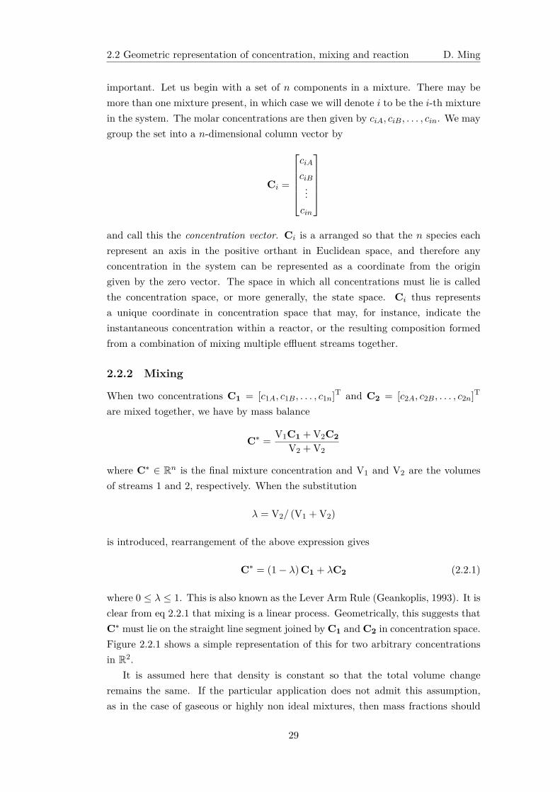
2.2 Geometric representation of concentration, mixing and reaction D. Ming
important. Let us begin with a set of n components in a mixture. There may bemore than one mixture present, in which case we will denote i to be the i-th mixturein the system. The molar concentrations are then given by ciA, ciB, . . . , cin. We maygroup the set into a n-dimensional column vector by
Ci =
ciA
ciB...cin
and call this the concentration vector. Ci is a arranged so that the n species eachrepresent an axis in the positive orthant in Euclidean space, and therefore anyconcentration in the system can be represented as a coordinate from the origingiven by the zero vector. The space in which all concentrations must lie is calledthe concentration space, or more generally, the state space. Ci thus representsa unique coordinate in concentration space that may, for instance, indicate theinstantaneous concentration within a reactor, or the resulting composition formedfrom a combination of mixing multiple effluent streams together.
2.2.2 Mixing
When two concentrations C1 = [c1A, c1B, . . . , c1n]T and C2 = [c2A, c2B, . . . , c2n]
T
are mixed together, we have by mass balance
C∗ =V1C1 + V2C2
V2 + V2
where C∗ ∈ Rn is the final mixture concentration and V1 and V2 are the volumesof streams 1 and 2, respectively. When the substitution
λ = V2/ (V1 + V2)
is introduced, rearrangement of the above expression gives
C∗ = (1− λ)C1 + λC2 (2.2.1)
where 0 ≤ λ ≤ 1. This is also known as the Lever Arm Rule (Geankoplis, 1993). It isclear from eq 2.2.1 that mixing is a linear process. Geometrically, this suggests thatC∗ must lie on the straight line segment joined by C1 and C2 in concentration space.Figure 2.2.1 shows a simple representation of this for two arbitrary concentrationsin R2.
It is assumed here that density is constant so that the total volume changeremains the same. If the particular application does not admit this assumption,as in the case of gaseous or highly non ideal mixtures, then mass fractions should
29
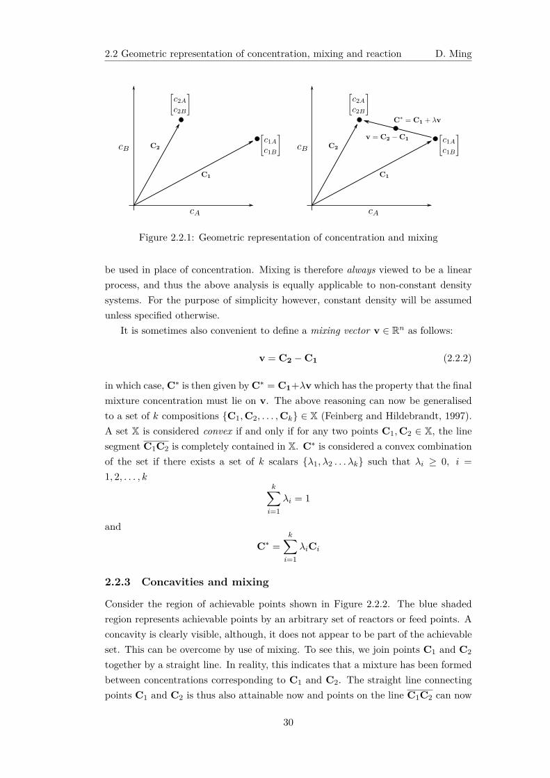
2.2 Geometric representation of concentration, mixing and reaction D. Ming
Figure 2.2.1: Geometric representation of concentration and mixing
be used in place of concentration. Mixing is therefore always viewed to be a linearprocess, and thus the above analysis is equally applicable to non-constant densitysystems. For the purpose of simplicity however, constant density will be assumedunless specified otherwise.
It is sometimes also convenient to define a mixing vector v ∈ Rn as follows:
v = C2 − C1 (2.2.2)
in which case, C∗ is then given by C∗ = C1+λv which has the property that the finalmixture concentration must lie on v. The above reasoning can now be generalisedto a set of k compositions {C1,C2, . . . ,Ck} ∈ X (Feinberg and Hildebrandt, 1997).A set X is considered convex if and only if for any two points C1,C2 ∈ X, the linesegment C1C2 is completely contained in X. C∗ is considered a convex combinationof the set if there exists a set of k scalars {λ1, λ2 . . . λk} such that λi ≥ 0, i =
1, 2, . . . , kk∑
i=1
λi = 1
and
C∗ =k∑
i=1
λiCi
2.2.3 Concavities and mixing
Consider the region of achievable points shown in Figure 2.2.2. The blue shadedregion represents achievable points by an arbitrary set of reactors or feed points. Aconcavity is clearly visible, although, it does not appear to be part of the achievableset. This can be overcome by use of mixing. To see this, we join points C1 and C2
together by a straight line. In reality, this indicates that a mixture has been formedbetween concentrations corresponding to C1 and C2. The straight line connectingpoints C1 and C2 is thus also attainable now and points on the line C1C2 can now
30
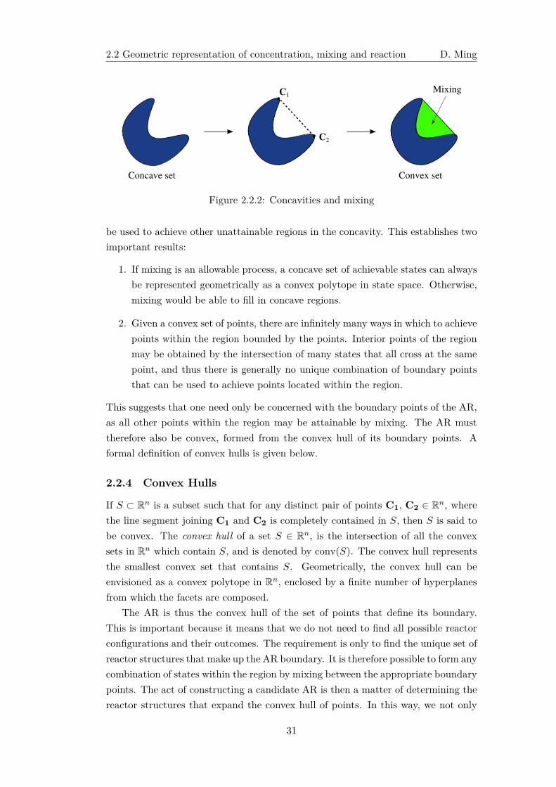
2.2 Geometric representation of concentration, mixing and reaction D. Ming
Concave set Convex set
Mixing
C2
C1
Figure 2.2.2: Concavities and mixing
be used to achieve other unattainable regions in the concavity. This establishes twoimportant results:
1. If mixing is an allowable process, a concave set of achievable states can alwaysbe represented geometrically as a convex polytope in state space. Otherwise,mixing would be able to fill in concave regions.
2. Given a convex set of points, there are infinitely many ways in which to achievepoints within the region bounded by the points. Interior points of the regionmay be obtained by the intersection of many states that all cross at the samepoint, and thus there is generally no unique combination of boundary pointsthat can be used to achieve points located within the region.
This suggests that one need only be concerned with the boundary points of the AR,as all other points within the region may be attainable by mixing. The AR musttherefore also be convex, formed from the convex hull of its boundary points. Aformal definition of convex hulls is given below.
2.2.4 Convex Hulls
If S ⊂ Rn is a subset such that for any distinct pair of points C1, C2 ∈ Rn, wherethe line segment joining C1 and C2 is completely contained in S, then S is said tobe convex. The convex hull of a set S ∈ Rn, is the intersection of all the convexsets in Rn which contain S, and is denoted by conv(S). The convex hull representsthe smallest convex set that contains S. Geometrically, the convex hull can beenvisioned as a convex polytope in Rn, enclosed by a finite number of hyperplanesfrom which the facets are composed.
The AR is thus the convex hull of the set of points that define its boundary.This is important because it means that we do not need to find all possible reactorconfigurations and their outcomes. The requirement is only to find the unique set ofreactor structures that make up the AR boundary. It is therefore possible to form anycombination of states within the region by mixing between the appropriate boundarypoints. The act of constructing a candidate AR is then a matter of determining thereactor structures that expand the convex hull of points. In this way, we not only
31
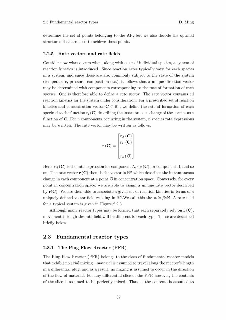
2.3 Fundamental reactor types D. Ming
determine the set of points belonging to the AR, but we also decode the optimalstructures that are used to achieve these points.
2.2.5 Rate vectors and rate fields
Consider now what occurs when, along with a set of individual species, a system ofreaction kinetics is introduced. Since reaction rates typically vary for each speciesin a system, and since these are also commonly subject to the state of the system(temperature, pressure, composition etc.), it follows that a unique direction vectormay be determined with components corresponding to the rate of formation of eachspecies. One is therefore able to define a rate vector. The rate vector contains allreaction kinetics for the system under consideration. For a prescribed set of reactionkinetics and concentration vector C ∈ Rn, we define the rate of formation of eachspecies i as the function ri (C) describing the instantaneous change of the species as afunction of C. For n components occurring in the system, n species rate expressionsmay be written. The rate vector may be written as follows:
r (C) =
rA (C)
rB (C)...
rn (C)
Here, rA (C) is the rate expression for component A, rB (C) for component B, and soon. The rate vector r (C) then, is the vector in Rn which describes the instantaneouschange in each component at a point C in concentration space. Conversely, for everypoint in concentration space, we are able to assign a unique rate vector describedby r(C). We are then able to associate a given set of reaction kinetics in terms of auniquely defined vector field residing in Rn.We call this the rate field. A rate fieldfor a typical system is given in Figure 2.2.3.
Although many reactor types may be formed that each separately rely on r (C),movement through the rate field will be different for each type. These are describedbriefly below.
2.3 Fundamental reactor types
2.3.1 The Plug Flow Reactor (PFR)
The Plug Flow Reactor (PFR) belongs to the class of fundamental reactor modelsthat exhibit no axial mixing – material is assumed to travel along the reactor’s lengthin a differential plug, and as a result, no mixing is assumed to occur in the directionof the flow of material. For any differential slice of the PFR however, the contentsof the slice is assumed to be perfectly mixed. That is, the contents is assumed to
32
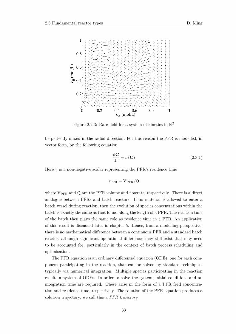
2.3 Fundamental reactor types D. Ming
Figure 2.2.3: Rate field for a system of kinetics in R2
be perfectly mixed in the radial direction. For this reason the PFR is modelled, invector form, by the following equation
dCdτ = r (C) (2.3.1)
Here τ is a non-negative scalar representing the PFR’s residence time
τPFR = VPFR/Q
where VPFR and Q are the PFR volume and flowrate, respectively. There is a directanalogue between PFRs and batch reactors. If no material is allowed to enter abatch vessel during reaction, then the evolution of species concentrations within thebatch is exactly the same as that found along the length of a PFR. The reaction timeof the batch then plays the same role as residence time in a PFR. An applicationof this result is discussed later in chapter 5. Hence, from a modelling perspective,there is no mathematical difference between a continuous PFR and a standard batchreactor, although significant operational differences may still exist that may needto be accounted for, particularly in the context of batch process scheduling andoptimisation.
The PFR equation is an ordinary differential equation (ODE), one for each com-ponent participating in the reaction, that can be solved by standard techniques,typically via numerical integration. Multiple species participating in the reactionresults a system of ODEs. In order to solve the system, initial conditions and anintegration time are required. These arise in the form of a PFR feed concentra-tion and residence time, respectively. The solution of the PFR equation produces asolution trajectory; we call this a PFR trajectory.
33
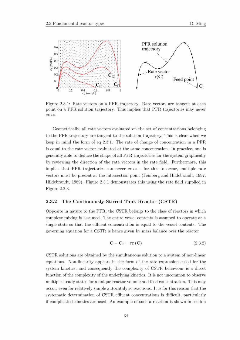
2.3 Fundamental reactor types D. Ming
Cf3
Cf2
Cf1
Rate vectorFeed point
PFR solutiontrajectory
Cf
r(C)
Figure 2.3.1: Rate vectors on a PFR trajectory. Rate vectors are tangent at eachpoint on a PFR solution trajectory. This implies that PFR trajectories may nevercross.
Geometrically, all rate vectors evaluated on the set of concentrations belongingto the PFR trajectory are tangent to the solution trajectory. This is clear when wekeep in mind the form of eq 2.3.1. The rate of change of concentration in a PFRis equal to the rate vector evaluated at the same concentration. In practice, one isgenerally able to deduce the shape of all PFR trajectories for the system graphicallyby reviewing the direction of the rate vectors in the rate field. Furthermore, thisimplies that PFR trajectories can never cross – for this to occur, multiple ratevectors must be present at the intersection point (Feinberg and Hildebrandt, 1997;Hildebrandt, 1989). Figure 2.3.1 demonstrates this using the rate field supplied inFigure 2.2.3.
2.3.2 The Continuously-Stirred Tank Reactor (CSTR)
Opposite in nature to the PFR, the CSTR belongs to the class of reactors in whichcomplete mixing is assumed. The entire vessel contents is assumed to operate at asingle state so that the effluent concentration is equal to the vessel contents. Thegoverning equation for a CSTR is hence given by mass balance over the reactor
C − Cf = τr (C) (2.3.2)
CSTR solutions are obtained by the simultaneous solution to a system of non-linearequations. Non-linearity appears in the form of the rate expressions used for thesystem kinetics, and consequently the complexity of CSTR behaviour is a directfunction of the complexity of the underlying kinetics. It is not uncommon to observemultiple steady states for a unique reactor volume and feed concentration. This mayoccur, even for relatively simple autocatalytic reactions. It is for this reason that thesystematic determination of CSTR effluent concentrations is difficult, particularlyif complicated kinetics are used. An example of such a reaction is shown in section
34
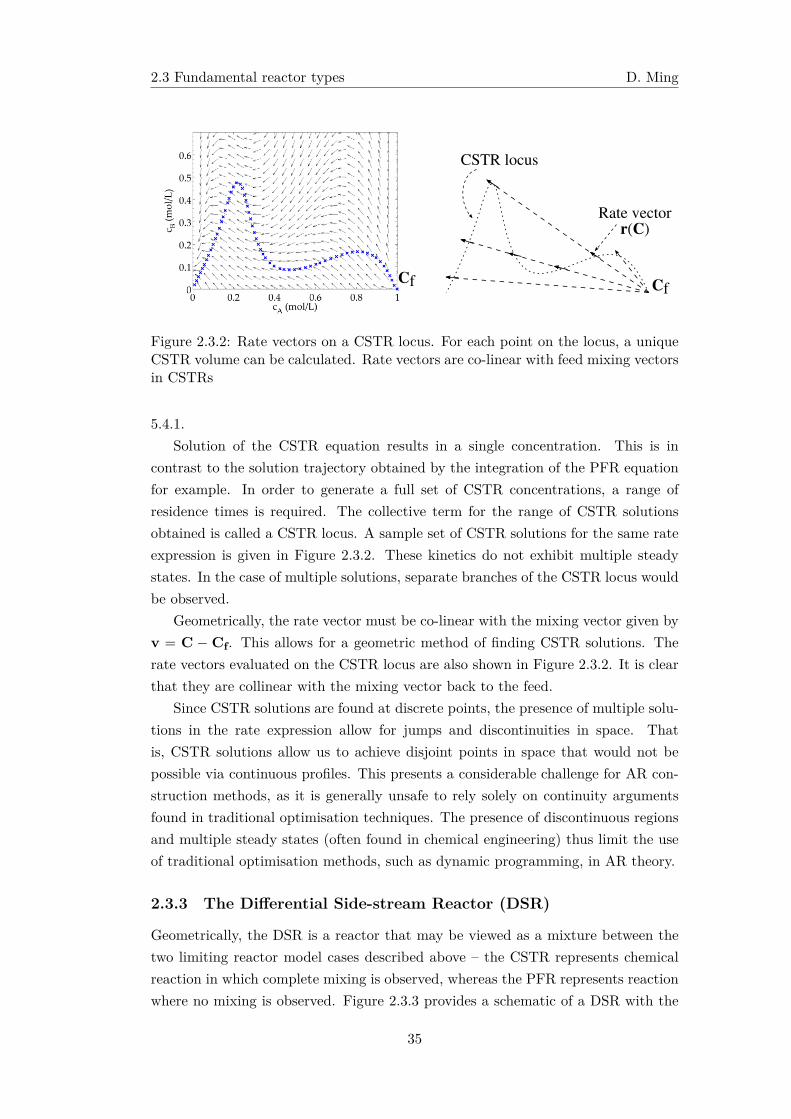
2.3 Fundamental reactor types D. Ming
Cf Cf
CSTR locus
Rate vectorr(C)
Figure 2.3.2: Rate vectors on a CSTR locus. For each point on the locus, a uniqueCSTR volume can be calculated. Rate vectors are co-linear with feed mixing vectorsin CSTRs
5.4.1.Solution of the CSTR equation results in a single concentration. This is in
contrast to the solution trajectory obtained by the integration of the PFR equationfor example. In order to generate a full set of CSTR concentrations, a range ofresidence times is required. The collective term for the range of CSTR solutionsobtained is called a CSTR locus. A sample set of CSTR solutions for the same rateexpression is given in Figure 2.3.2. These kinetics do not exhibit multiple steadystates. In the case of multiple solutions, separate branches of the CSTR locus wouldbe observed.
Geometrically, the rate vector must be co-linear with the mixing vector given byv = C − Cf. This allows for a geometric method of finding CSTR solutions. Therate vectors evaluated on the CSTR locus are also shown in Figure 2.3.2. It is clearthat they are collinear with the mixing vector back to the feed.
Since CSTR solutions are found at discrete points, the presence of multiple solu-tions in the rate expression allow for jumps and discontinuities in space. Thatis, CSTR solutions allow us to achieve disjoint points in space that would not bepossible via continuous profiles. This presents a considerable challenge for AR con-struction methods, as it is generally unsafe to rely solely on continuity argumentsfound in traditional optimisation techniques. The presence of discontinuous regionsand multiple steady states (often found in chemical engineering) thus limit the useof traditional optimisation methods, such as dynamic programming, in AR theory.
2.3.3 The Differential Side-stream Reactor (DSR)
Geometrically, the DSR is a reactor that may be viewed as a mixture between thetwo limiting reactor model cases described above – the CSTR represents chemicalreaction in which complete mixing is observed, whereas the PFR represents reactionwhere no mixing is observed. Figure 2.3.3 provides a schematic of a DSR with the
35
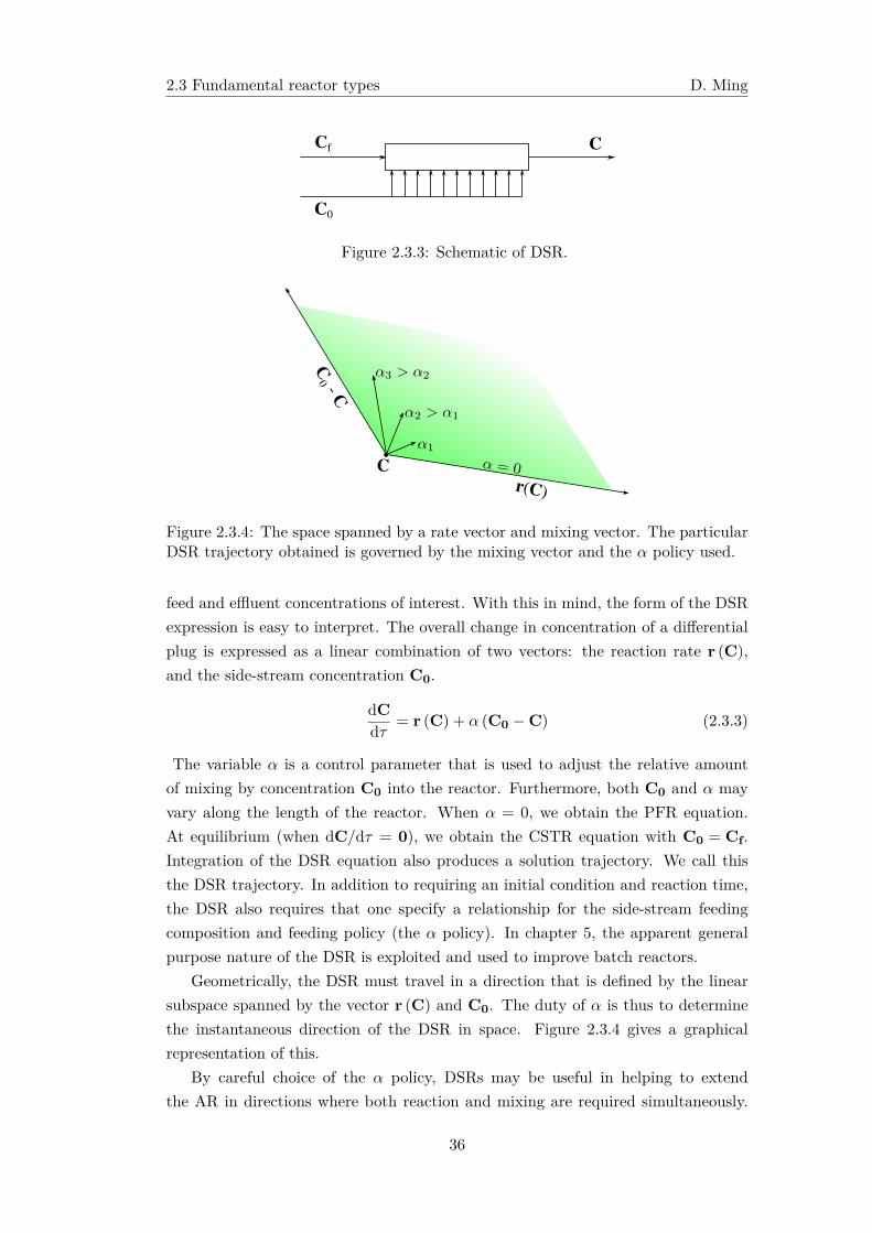
2.3 Fundamental reactor types D. Ming
CCf
C0
Figure 2.3.3: Schematic of DSR.
r(C)C
C0 - C
Figure 2.3.4: The space spanned by a rate vector and mixing vector. The particularDSR trajectory obtained is governed by the mixing vector and the α policy used.
feed and effluent concentrations of interest. With this in mind, the form of the DSRexpression is easy to interpret. The overall change in concentration of a differentialplug is expressed as a linear combination of two vectors: the reaction rate r (C),and the side-stream concentration C0.
dCdτ = r (C) + α (C0 − C) (2.3.3)
The variable α is a control parameter that is used to adjust the relative amountof mixing by concentration C0 into the reactor. Furthermore, both C0 and α mayvary along the length of the reactor. When α = 0, we obtain the PFR equation.At equilibrium (when dC/dτ = 0), we obtain the CSTR equation with C0 = Cf.Integration of the DSR equation also produces a solution trajectory. We call thisthe DSR trajectory. In addition to requiring an initial condition and reaction time,the DSR also requires that one specify a relationship for the side-stream feedingcomposition and feeding policy (the α policy). In chapter 5, the apparent generalpurpose nature of the DSR is exploited and used to improve batch reactors.
Geometrically, the DSR must travel in a direction that is defined by the linearsubspace spanned by the vector r (C) and C0. The duty of α is thus to determinethe instantaneous direction of the DSR in space. Figure 2.3.4 gives a graphicalrepresentation of this.
By careful choice of the α policy, DSRs may be useful in helping to extendthe AR in directions where both reaction and mixing are required simultaneously.
36
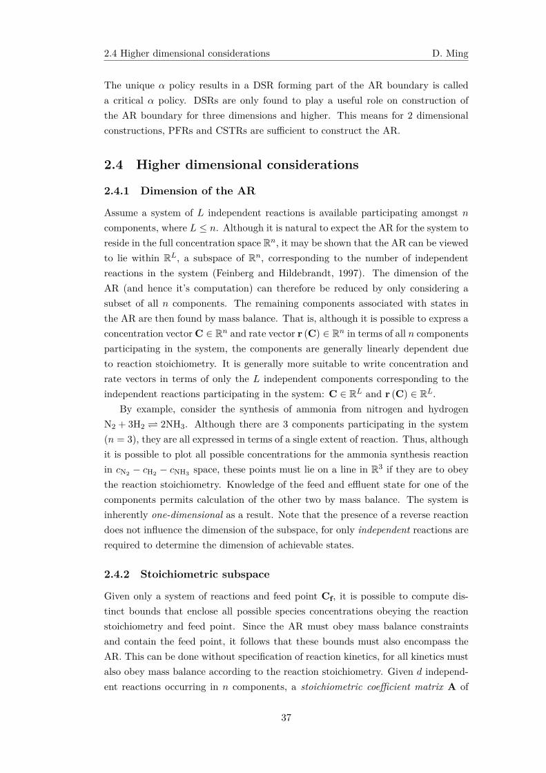
2.4 Higher dimensional considerations D. Ming
The unique α policy results in a DSR forming part of the AR boundary is calleda critical α policy. DSRs are only found to play a useful role on construction ofthe AR boundary for three dimensions and higher. This means for 2 dimensionalconstructions, PFRs and CSTRs are sufficient to construct the AR.
2.4 Higher dimensional considerations
2.4.1 Dimension of the AR
Assume a system of L independent reactions is available participating amongst n
components, where L ≤ n. Although it is natural to expect the AR for the system toreside in the full concentration space Rn, it may be shown that the AR can be viewedto lie within RL, a subspace of Rn, corresponding to the number of independentreactions in the system (Feinberg and Hildebrandt, 1997). The dimension of theAR (and hence it’s computation) can therefore be reduced by only considering asubset of all n components. The remaining components associated with states inthe AR are then found by mass balance. That is, although it is possible to express aconcentration vector C ∈ Rn and rate vector r (C) ∈ Rn in terms of all n componentsparticipating in the system, the components are generally linearly dependent dueto reaction stoichiometry. It is generally more suitable to write concentration andrate vectors in terms of only the L independent components corresponding to theindependent reactions participating in the system: C ∈ RL and r (C) ∈ RL.
By example, consider the synthesis of ammonia from nitrogen and hydrogenN2 + 3H2 2NH3. Although there are 3 components participating in the system(n = 3), they are all expressed in terms of a single extent of reaction. Thus, althoughit is possible to plot all possible concentrations for the ammonia synthesis reactionin cN2 − cH2 − cNH3 space, these points must lie on a line in R3 if they are to obeythe reaction stoichiometry. Knowledge of the feed and effluent state for one of thecomponents permits calculation of the other two by mass balance. The system isinherently one-dimensional as a result. Note that the presence of a reverse reactiondoes not influence the dimension of the subspace, for only independent reactions arerequired to determine the dimension of achievable states.
2.4.2 Stoichiometric subspace
Given only a system of reactions and feed point Cf, it is possible to compute dis-tinct bounds that enclose all possible species concentrations obeying the reactionstoichiometry and feed point. Since the AR must obey mass balance constraintsand contain the feed point, it follows that these bounds must also encompass theAR. This can be done without specification of reaction kinetics, for all kinetics mustalso obey mass balance according to the reaction stoichiometry. Given d independ-ent reactions occurring in n components, a stoichiometric coefficient matrix A of
37
2.4 Higher dimensional considerations D. Ming
size (n× d) can be formed, housing the species reaction coefficients participating ineach reaction in the system
A =
ν11 · · · νd1... . . . ...
ν1n · · · νdn
where νij is the stoichiometric coefficient of component i participating in reactionj. It is straightforward to show how all species concentrations C in the system canbe expressed in terms of linear combination of an initial feed vector Cf and thestoichiometric coefficient matrix A
C = Cf + Aε (2.4.1a)
ε is a (d× 1) vector corresponding to each extent of reaction. Indeed, the columnsof A correspond to the individual reactions participating in the system. The spacespanned by eq 2.4.1a is hence determined by A offset by Cf. Furthermore, feasibleconcentrations must also be non-negative
C ≥ 0 (2.4.1b)
Concentrations obeying eq 2.4.1a and eq 2.4.1b are said to be stoichiometricallycompatible with the feed point Cf. We term the space spanned by eq 2.4.1a thestoichiometric subspace and often denoted by the symbol S. The dimension of S ishence determined by the dimension of A, in particular. This provides a simple wayof calculating the dimension of the stoichiometric subspace since this is equivalentto finding the rank of A, rank (A). If there are d independent reactions, it followsthat rank (A) = d.
In section 2.4.1, we discussed how the AR exists as a subspace of Rn. The dimen-sion of this space is determined by the number of independent reactions present inthe system. Computing the dimension of the AR is hence achieved by computationof the stoichiometric subspace, which is directly related to the number of independ-ent reactions, from rank (A). Since AR theory has typically come about from 2Dconstructions, the stoichiometric subspace is generally represented as a triangle. Itis for this reason that the stoichiometric subspace is commonly also referred to asthe mass balance triangle. A worked example demonstrating how to compute thestoichiometric subspace given reaction stoichiometry and a feed is given in AppendixB.2.
2.4.3 PFRs on the AR boundary
From section 2.2.3, a concave set of achievable points can always be made convexthrough mixing. A set X containing k points produced by a reactive network will
38
2.4 Higher dimensional considerations D. Ming
have points in or on the boundary defined by the convex hull of X, conv (X). If apoint Ci satisfies the relation
Ci = λ1C1 + λ2C2 + · · ·+ λkCk
in which at least one of the λ’s is non-negative, then Ci must lie on the interior ofa line segment joining points in X. Hence, Ci can be formed from a mixture of theboundary points in X given by conv (X). It follows that if a point Ci can be formedfrom a mixture of two or more other points, then it cannot be an extreme point ofconv (X) and thus it also cannot be formed as a result of reaction. From this, we notethat the extreme points of X are those that arise from reaction alone, for otherwisethey would satisfy the above mixing relation. It follows that the boundary of the ARis generated from reaction and mixing processes only. Linear (flat) sections of theAR boundary are those resulting from mixing process whereas as convex (curved)sections of the boundary are those generated from reaction alone.
An important result of this arises in the form of theorem 1 in Feinberg andHildebrandt (1997). Using the above result, along with the complement principlediscussed in chapter 1, the theorem states that any set of extreme points disjointfrom the feed are the result of the union of PFR trajectories (solutions to eq 2.3.1).Though the AR boundary may typically be composed of a complex set of multiplereactor types with intermediate mixing, the final reactor type used to achieve ex-treme points on the AR boundary arise from PFR trajectories alone. This is usefulas a design guideline in reactor network synthesis problems, for terminating reactortype will always be that of a PFR.
2.4.4 Connectors and critical reactors
Connectors
Although it is known that only PFR trajectories produce extreme points on the ARboundary, other special reactor types must be employed in order to reach them. Aconnector is used in the terminology of AR theory to describe a special manifoldof points residing on the AR boundary which allow for connection to the manifoldof extreme PFR trajectories. In Feinberg (2000b), they are described as ‘serviceroads’ that link to PFR highways. Although a precise mathematical definition ofconnectors can be found in Feinberg and Hildebrandt (1997), it is sufficient for oursake to only have a qualitative understanding of their duty in the formation of theAR boundary. In simple terms, connectors are points on the AR boundary whichare disjoint from the feed that originate from mixing lines. Connectors leave mixinglines to connect to PFR trajectories smoothly. Moreover, connectors are formedspecifically from the solution of the CSTR and DSR equations only.
39
2.4 Higher dimensional considerations D. Ming
Critical DSRs
A DSR solution trajectory contained entirely on the AR boundary is termed a crit-ical DSR trajectory. Critical DSR trajectories result from highly specific α feedingpolicies, termed critical α policies, that allow for traversal on the AR boundary.Critical DSR trajectories act as connectors to PFR trajectories on the boundary. Inorder to understand why these are special, we must understand that the AR bound-ary plays special physical significance in the context of achievability. By simplyresiding on the boundary, the corresponding reactor must be controlled in a highlyspecialised manner.
It is possible to compute critical α policies from this understanding using ideasfrom geometric control theory (Feinberg, 1999). To see this, suppose that a criticalDSR trajectory is available, controlled by a critical α policy. Since it is critical, itmust lie entirely on the AR boundary. Since it resides on the boundary, it bor-ders between all achievable states to all unachievable states. If a perturbation isintroduced into the control policy, then the resulting trajectory will deviate fromthe path prescribed by the critical trajectory. Since the trajectory is critical, thisperturbation may serve only to produce a deviation into the AR, for else the originalDSR trajectory would not be critical in the first place. We can see from this thatcontrollability arguments dictate the form of critical DSR trajectories and hencethe computation of critical α policies. Indeed, whereas we often attempt to seekcompletely controllable solution trajectories in practice, it is the absence of controlthat must be used as a condition for residing on the AR boundary (Feinberg, 1999).In the theory of optimal control, the resulting α policy corresponds to a singularcontrol profile.
A condition for computing critical reactors is then possible. Since the nature ofthe DSR equation is inherently non-linear, the use of iterated Lie Brackets is requiredin order to calculate the condition. Specifically, rewriting the DSR equation in theform
f (C) = r (C) + αv (C)
wherev (C) = C − C0
we may then define the Lie bracket, z[1] (C), in terms of f (C) and v (C)
z[1] (C) = [f (C) ,v (C)]
= dv (C) f (C)− df (C)v (C)
where df (C), dv (C) and dz[i] (C) are the Jacobians of vector functions f (C), v (C)
and z[i] (C), respectively. From this we may define iterated Lie brackets
z[2] (C) =[f (C) , z[1] (C)
]40
2.4 Higher dimensional considerations D. Ming
= dz[1] (C) f (C)− df (C) z[1] (C)
which may be generalised in a recursive fashion
z[k] (C) =[f (C) , z[k−1] (C)
]= dz[k−1] (C) f (C)− df (C) z[k−1] (C)
It is then possible to show that for a DSR to produce effluent concentrations thatreside on the AR boundary, vectors
{f (C) ,v (C) , z[1] (C) , . . . , z[k] (C)
}must be
linearly dependent. In practice, this is achieved by computing the determinant ofthe matrix whose columns are composed of the above vectors as well as vectors form-ing an orthogonal basis to the stoichiometric subspace S, and setting the resultingexpression to zero:
Det[f (C) ,v (C) , z[1] (C) , z[2], . . . , z[k],N
]= 0 (2.4.2)
Here, N is a matrix containing columns orthogonal to S. Note that we only providethese definitions here for completeness. A detailed description of the procedure,with worked examples, can again be found in (Feinberg, 2000b). Even if we donot wish to know specific details of the method, it is still possible to understandthe general procedure: observe that eq 2.4.2 is in fact a function of α. Solutionand rearrangement of eq 2.4.2 may then be used to determine a critical α policycorresponding to a critical DSR.
An important consequence of the fact that critical DSR trajectories must lieentirely on the AR boundary is that these trajectories must then also originate onthe boundary. Thus points on the true AR boundary must be used as starting pointsfor critical DSRs. This places a large constraint on the number of possible initiatingpoints for critical DSR trajectories. Furthermore, the side-stream concentration C0
is also specialised. Similar to starting points of critical trajectories, C0 must also besourced from extreme points on the AR boundary. This again places a limitation onthe possible side-stream concentrations used in critical DSRs, and raises questionsas to how one should search for these during construction, when the full AR has notbeen identified yet. In practice, the value of C0 is often taken to be the same of thefeed point C0 = Cf.
Critical CSTRs
The above control arguments may now be extended to include critical CSTRs. Sup-pose that a CSTR is available that produces effluent concentrations on the ARboundary (it is a critical CSTR). If a DSR is connected in series directly after theCSTR, then the DSR must also start on the AR boundary. In order for the DSRto also be critical, it’s trajectory must satisfy eq 2.4.2. This provides a link for
41
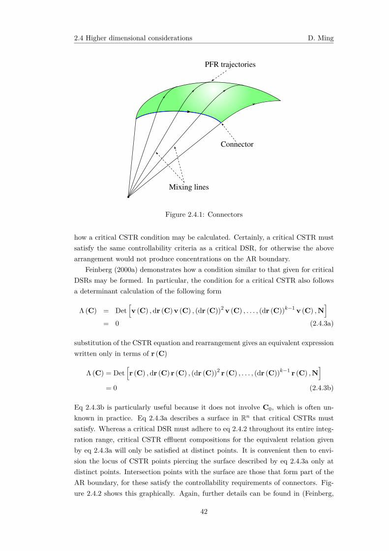
2.4 Higher dimensional considerations D. Ming
PFR trajectories
Mixing lines
Connector
Figure 2.4.1: Connectors
how a critical CSTR condition may be calculated. Certainly, a critical CSTR mustsatisfy the same controllability criteria as a critical DSR, for otherwise the abovearrangement would not produce concentrations on the AR boundary.
Feinberg (2000a) demonstrates how a condition similar to that given for criticalDSRs may be formed. In particular, the condition for a critical CSTR also followsa determinant calculation of the following form
Λ (C) = Det[v (C) ,dr (C)v (C) , (dr (C))2 v (C) , . . . , (dr (C))k−1 v (C) ,N
]= 0 (2.4.3a)
substitution of the CSTR equation and rearrangement gives an equivalent expressionwritten only in terms of r (C)
Λ (C) = Det[r (C) ,dr (C) r (C) , (dr (C))2 r (C) , . . . , (dr (C))k−1 r (C) ,N
]= 0 (2.4.3b)
Eq 2.4.3b is particularly useful because it does not involve C0, which is often un-known in practice. Eq 2.4.3a describes a surface in Rn that critical CSTRs mustsatisfy. Whereas a critical DSR must adhere to eq 2.4.2 throughout its entire integ-ration range, critical CSTR effluent compositions for the equivalent relation givenby eq 2.4.3a will only be satisfied at distinct points. It is convenient then to envi-sion the locus of CSTR points piercing the surface described by eq 2.4.3a only atdistinct points. Intersection points with the surface are those that form part of theAR boundary, for these satisfy the controllability requirements of connectors. Fig-ure 2.4.2 shows this graphically. Again, further details can be found in (Feinberg,
42
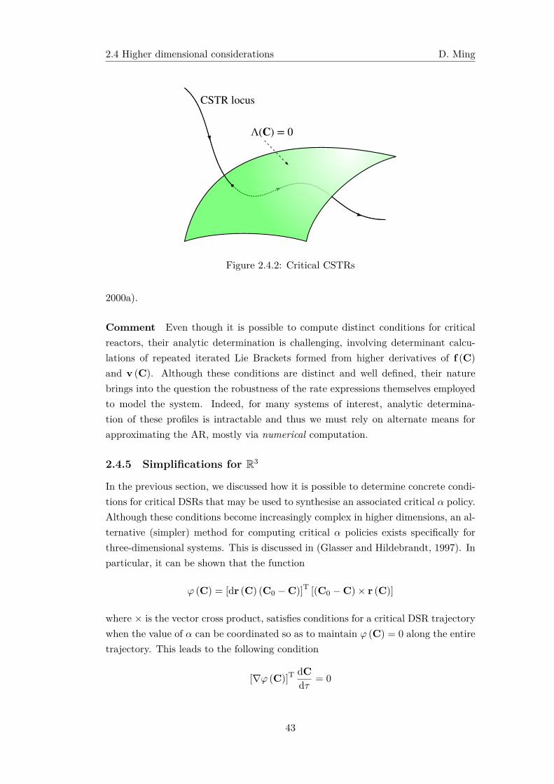
2.4 Higher dimensional considerations D. Ming
CSTR locus
Λ(C) = 0
Figure 2.4.2: Critical CSTRs
2000a).
Comment Even though it is possible to compute distinct conditions for criticalreactors, their analytic determination is challenging, involving determinant calcu-lations of repeated iterated Lie Brackets formed from higher derivatives of f (C)
and v (C). Although these conditions are distinct and well defined, their naturebrings into the question the robustness of the rate expressions themselves employedto model the system. Indeed, for many systems of interest, analytic determina-tion of these profiles is intractable and thus we must rely on alternate means forapproximating the AR, mostly via numerical computation.
2.4.5 Simplifications for R3
In the previous section, we discussed how it is possible to determine concrete condi-tions for critical DSRs that may be used to synthesise an associated critical α policy.Although these conditions become increasingly complex in higher dimensions, an al-ternative (simpler) method for computing critical α policies exists specifically forthree-dimensional systems. This is discussed in (Glasser and Hildebrandt, 1997). Inparticular, it can be shown that the function
φ (C) = [dr (C) (C0 − C)]T [(C0 − C)× r (C)]
where × is the vector cross product, satisfies conditions for a critical DSR trajectorywhen the value of α can be coordinated so as to maintain φ (C) = 0 along the entiretrajectory. This leads to the following condition
[∇φ (C)]TdCdτ = 0
43
2.5 AR construction from fundamental processes D. Ming
where ∇φ (C) is the gradient of the scalar function φ (C), and dC/dτ is the vec-tor differential equation describing the DSR expression. Substituting eq 2.3.3 andfurther simplification leads to an explicit expression for α
α = − [∇φ (C)]T r (C)
[∇φ (C)]T (C0 − C)(2.4.4)
The scalar function given by eq 2.4.4 represents a critical α policy for systems in R3
specifically. This result is commonly referred to as the ‘VdelR’ condition.
2.5 AR construction from fundamental processes
Once the fundamental process vectors of reaction and mixing are known, AR con-struction may begin. By optimal structures, we mean the reactor configurationsthat are able to expand the region of attainable points in the greatest manner pos-sible. The convex hull of these points is then the AR. Since all interior points can beachieved by mixing, only boundary points are required to achieve all points in theregion. Hence, the task of finding the AR reduces to finding the unique set of struc-tures that form its boundary. The solution to subsequent optimisation problemsthus only involves combinations of these optimal structures with mixing.
2.5.1 General procedure for constructing the AR
Unless the system kinetics under consideration is simple, AR construction is cur-rently still not straightforward, requiring previous AR knowledge and constructionexperience. In general, a fair amount of time and skill is involved whenever theAR for a system is to be determined. AR practitioners often spend a large amountof time visualising and interpreting the AR boundary to identify sections for howto expand the candidate region further. Nevertheless, even if the full AR cannotbe determined, it is always possible to generate a candidate region representing alarge portion of the true AR. Although analytic determination of the AR is difficult,this does not prohibit the practice of a generalised, common-sense, approach to ARconstruction. Indeed, all constructions generally follow a similar procedure, evenif the final polytope is substantially different. A typical construction procedure isprovided below as a guideline for how one might generate at least a candidate AR.
Specify system kinetics and feed point (or convex hull of feed points)Since the AR is defined in terms of its kinetics and feed point, these must both beinitially specified. The system of reactions must be known along with the reactionstoichiometry. Specification of the feed point is usually determined by economic oroperating constraints. If there are more than one feed points available, then theconvex hull of all feed points is used as the initial candidate AR.
44
2.5 AR construction from fundamental processes D. Ming
Determine dimension of problem and (optional) stoichiometric subspace.From the reaction stoichiometry and feed point, it is possible to compute the dimen-sion of the problem by calculating the rank of the stoichiometric coefficient matrixA. This determines the complexity of the solution procedure: 2D problems willnot require DSRs or the calculation of critical reactors, 3D problems may exploitthe ‘VdelR’ condition of section 2.4.5 to determine critical α policies easier, andhigher dimensional problems will need to be visualised as projections onto differentcomponent spaces in R2 and R3.
It is also advantageous to compute the stoichiometric subspace from the reactionstoichiometry and feed point. This establishes limits in space in which the AR isknown to reside that may guide the search for other reactor structures that extendthe region.
Generate PFR trajectories and CSTR locus from the feed The simplestmethod for expanding the initial set of achievable concentrations is to determinethe PFR trajectory and CSTR locus from the feed points. Solving the PFR is de-termined by integration of a system of ordinary differential equations whereas theCSTR locus involves the solution of a system on non-linear equations. Dependingon the complexity of the rate expressions, multiple CSTR steady-states may existthat will also need to be accounted for. Otherwise, the full set of achievable concen-trations may not be discovered. Under certain reactions, the PFR trajectory maybe completely convex, indicating that a PFR from the feed is the optimal reactorstructure. In this case, construction may be terminated here as the convex hull ofthe PFR trajectory corresponds to the true AR. This situation, although seeminglyrare, is observed for linear kinetics (Glasser and Horn, 1980).
Every point on the CSTR locus may be used as an initiating point for a PFRtrajectory. From section 2.4.3, it is known that PFR trajectories make up the finalextreme points of the AR and therefore it is sensible to always include PFRs as thefinal reactor type. Thus PFR trajectories may be generated from all CSTR points.Once this has been achieved, the convex hull associated with the PFR trajectoriesand CSTR from the feed may be computed with a standard convex hull algorithm.The resulting polytope generally constitutes a reasonable first approximation to theAR.
Inspect the boundary for expansion The convex polytope resulting from PFRtrajectories and CSTR points may now be checked for possible extensions. Fortwo-dimensional systems, it is convenient to plot the rate field and overlay it ontothe region. In this way, we are able to visually inspect the candidate region forany possible rate vectors pointing out of the boundary. For higher dimensions, itmay be possible to visualise sections of the boundary and plot rate vectors in asimilar manner, however manipulation, visualisation and interpretation of the data
45
2.5 AR construction from fundamental processes D. Ming
is inherently more complex. Nevertheless, if rate vectors on the boundary can befound that point out of the region, then the region may be extended further withPFR trajectories from those particular boundary points. If it is difficult to inspectrate vectors on the boundary, then an attempt should be made to expand the regionby use of DSR trajectories.
Compute the critical α policy For systems involving three or more independ-ent reactions, the AR boundary may be composed of reactor structures containingcritical DSRs. The guidelines discussed in section 2.4.4 may be followed to computecritical α policies that may form part of the AR boundary. These expressions in-volve the evaluation and solution of iterated Lie brackets which, depending on thecomplexity of the rate expression and dimension of the system, may allow for ananalytic expression for the critical α policy. For systems specifically cast in R3, thecritical α policy may be determined by use of the ‘VdelR’ condition instead. Theparticular expression obtained for α will depend on the side-stream composition C0
specified. As already mentioned, C0 must originate from a point on the true ARboundary which may be difficult to know seeing as this precludes determination ofthe AR. In practice we often use C0 = Cf.
Once an expression for the critical α policy has been found, it can be substitutedinto the DSR expression and integrated given an appropriate initial condition. Initialpoints of integration for critical DSR trajectories are again constrained to lie on thetrue AR boundary, which is unknown up to this point. The feed set and equilibriumpoints from the CSTR locus and PFR trajectories are typically utilised in practice.
Compute the critical CSTR surface Λ (C) = 0 Connectors on the AR bound-ary might also arise from critical CSTR effluent compositions. Thus, determinationof the critical CSTR surface described by Λ (C) = 0 may also help to expand theregion. Eq 2.4.3b can be solved and plotted resulting in a surface in Rn. Eq 2.4.3bis often employed over eq 2.4.3a seeing as it does not involve specification of C0,which is also unknown. CSTR solutions that intersect the surface generated by eq2.4.3b are then critical CSTR solutions.
PFR trajectories from critical reactor solutions PFRs initiated from thecritical reactor effluent concentrations are special as these form part of the trueAR boundary. The resulting region generated by computing the convex hull ofall points generate up to this point represents a good approximation to the AR.Depending on whether the above steps are followed to completion, there may stillexist points that could expand the region further - often regions are obtained thatsatisfy all AR properties but which are not the true AR dues to multiple CSTRsteady-states. Again, analytic determination of the AR is often difficult, requiringmany visualisation and boundary interpretation steps in order to obtain a sense of
46
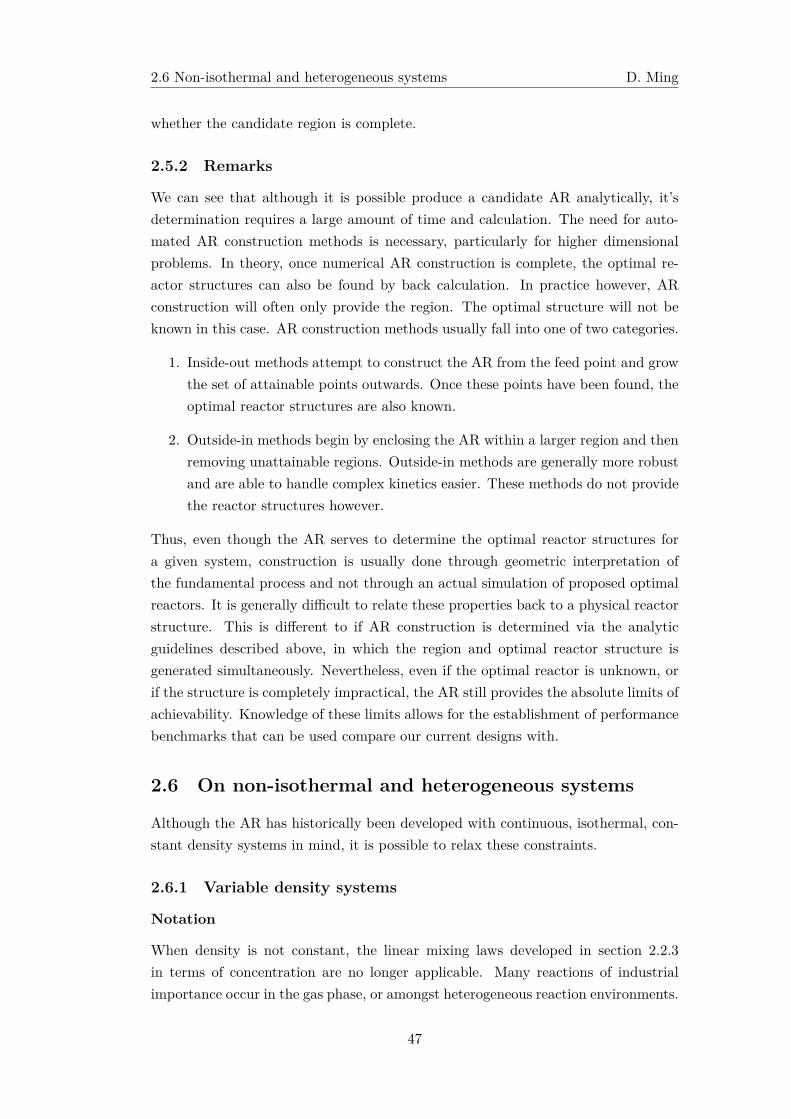
2.6 Non-isothermal and heterogeneous systems D. Ming
whether the candidate region is complete.
2.5.2 Remarks
We can see that although it is possible produce a candidate AR analytically, it’sdetermination requires a large amount of time and calculation. The need for auto-mated AR construction methods is necessary, particularly for higher dimensionalproblems. In theory, once numerical AR construction is complete, the optimal re-actor structures can also be found by back calculation. In practice however, ARconstruction will often only provide the region. The optimal structure will not beknown in this case. AR construction methods usually fall into one of two categories.
1. Inside-out methods attempt to construct the AR from the feed point and growthe set of attainable points outwards. Once these points have been found, theoptimal reactor structures are also known.
2. Outside-in methods begin by enclosing the AR within a larger region and thenremoving unattainable regions. Outside-in methods are generally more robustand are able to handle complex kinetics easier. These methods do not providethe reactor structures however.
Thus, even though the AR serves to determine the optimal reactor structures fora given system, construction is usually done through geometric interpretation ofthe fundamental process and not through an actual simulation of proposed optimalreactors. It is generally difficult to relate these properties back to a physical reactorstructure. This is different to if AR construction is determined via the analyticguidelines described above, in which the region and optimal reactor structure isgenerated simultaneously. Nevertheless, even if the optimal reactor is unknown, orif the structure is completely impractical, the AR still provides the absolute limits ofachievability. Knowledge of these limits allows for the establishment of performancebenchmarks that can be used compare our current designs with.
2.6 On non-isothermal and heterogeneous systems
Although the AR has historically been developed with continuous, isothermal, con-stant density systems in mind, it is possible to relax these constraints.
2.6.1 Variable density systems
Notation
When density is not constant, the linear mixing laws developed in section 2.2.3in terms of concentration are no longer applicable. Many reactions of industrialimportance occur in the gas phase, or amongst heterogeneous reaction environments.
47
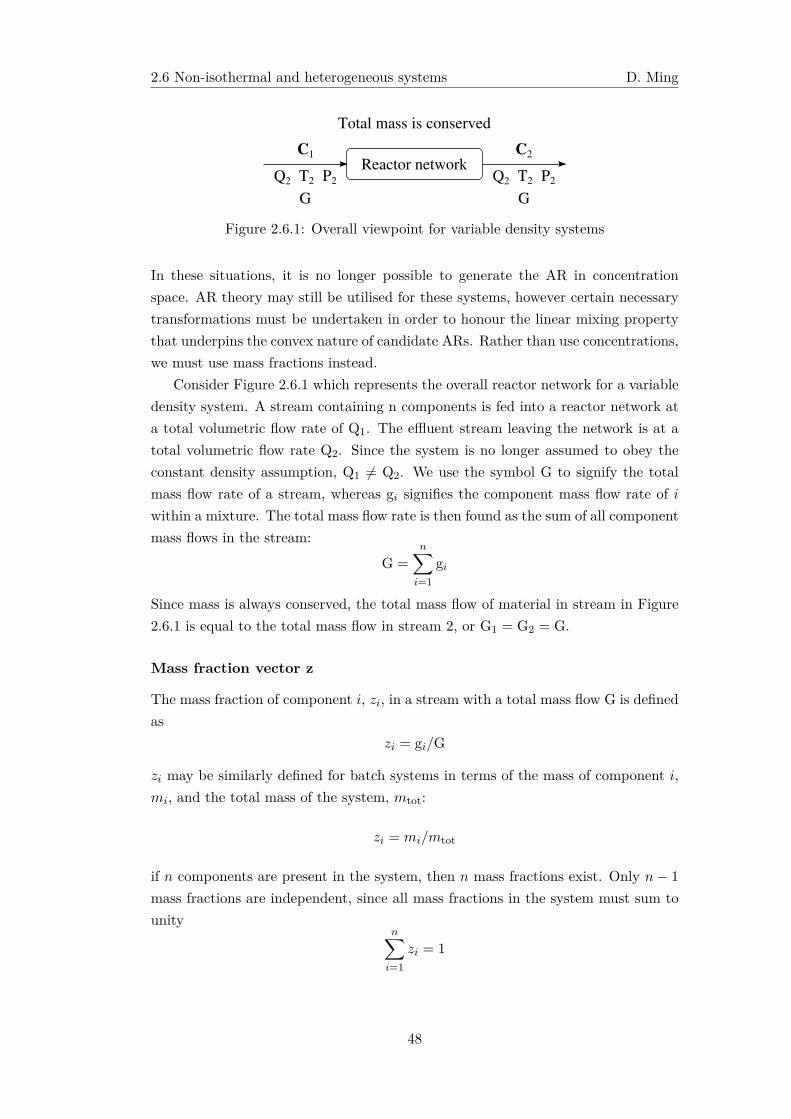
2.6 Non-isothermal and heterogeneous systems D. Ming
G G
Total mass is conservedC1
Q2 T2 P2Reactor network
C2
Q2 T2 P2
Figure 2.6.1: Overall viewpoint for variable density systems
In these situations, it is no longer possible to generate the AR in concentrationspace. AR theory may still be utilised for these systems, however certain necessarytransformations must be undertaken in order to honour the linear mixing propertythat underpins the convex nature of candidate ARs. Rather than use concentrations,we must use mass fractions instead.
Consider Figure 2.6.1 which represents the overall reactor network for a variabledensity system. A stream containing n components is fed into a reactor network ata total volumetric flow rate of Q1. The effluent stream leaving the network is at atotal volumetric flow rate Q2. Since the system is no longer assumed to obey theconstant density assumption, Q1 ̸= Q2. We use the symbol G to signify the totalmass flow rate of a stream, whereas gi signifies the component mass flow rate of iwithin a mixture. The total mass flow rate is then found as the sum of all componentmass flows in the stream:
G =
n∑i=1
gi
Since mass is always conserved, the total mass flow of material in stream in Figure2.6.1 is equal to the total mass flow in stream 2, or G1 = G2 = G.
Mass fraction vector z
The mass fraction of component i, zi, in a stream with a total mass flow G is definedas
zi = gi/G
zi may be similarly defined for batch systems in terms of the mass of component i,mi, and the total mass of the system, mtot:
zi = mi/mtot
if n components are present in the system, then n mass fractions exist. Only n− 1
mass fractions are independent, since all mass fractions in the system must sum tounity
n∑i=1
zi = 1
48
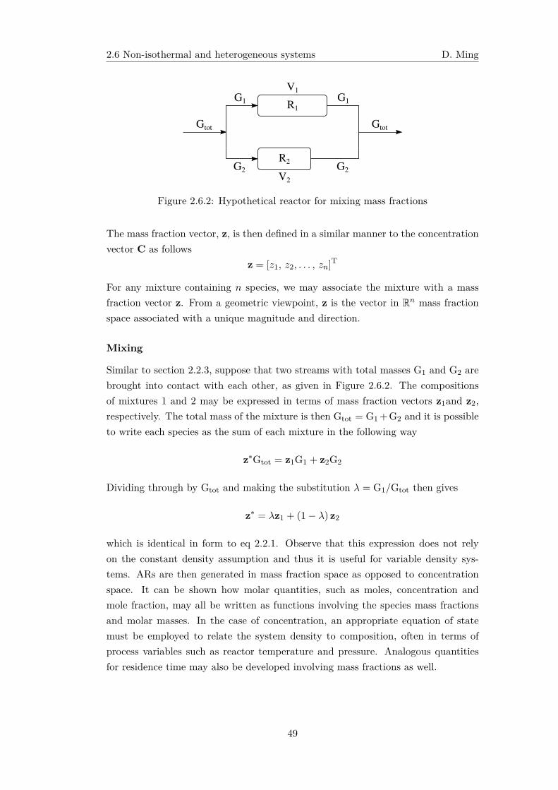
2.6 Non-isothermal and heterogeneous systems D. Ming
R2
R1
V1
V2
Gtot
G1
G2
G1
G2
Gtot
Figure 2.6.2: Hypothetical reactor for mixing mass fractions
The mass fraction vector, z, is then defined in a similar manner to the concentrationvector C as follows
z = [z1, z2, . . . , zn]T
For any mixture containing n species, we may associate the mixture with a massfraction vector z. From a geometric viewpoint, z is the vector in Rn mass fractionspace associated with a unique magnitude and direction.
Mixing
Similar to section 2.2.3, suppose that two streams with total masses G1 and G2 arebrought into contact with each other, as given in Figure 2.6.2. The compositionsof mixtures 1 and 2 may be expressed in terms of mass fraction vectors z1and z2,respectively. The total mass of the mixture is then Gtot = G1+G2 and it is possibleto write each species as the sum of each mixture in the following way
z∗Gtot = z1G1 + z2G2
Dividing through by Gtot and making the substitution λ = G1/Gtot then gives
z∗ = λz1 + (1− λ) z2
which is identical in form to eq 2.2.1. Observe that this expression does not relyon the constant density assumption and thus it is useful for variable density sys-tems. ARs are then generated in mass fraction space as opposed to concentrationspace. It can be shown how molar quantities, such as moles, concentration andmole fraction, may all be written as functions involving the species mass fractionsand molar masses. In the case of concentration, an appropriate equation of statemust be employed to relate the system density to composition, often in terms ofprocess variables such as reactor temperature and pressure. Analogous quantitiesfor residence time may also be developed involving mass fractions as well.
49
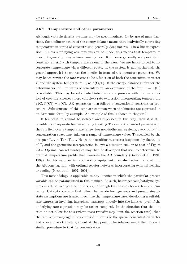
2.7 Conclusion D. Ming
2.6.2 Temperature and other parameters
Although variable density systems may be accommodated for by use of mass frac-tions, the nonlinear nature of the energy balance means that analytically expressingtemperature in terms of concentration generally does not result in a linear expres-sion. Unless simplifying assumptions can be made, this means that temperaturedoes not generally obey a linear mixing law. It it hence generally not possible toconstruct an AR with temperature as one of the axes. We are hence forced to in-corporate temperature via a different route. If the system is non-isothermal, thegeneral approach is to express the kinetics in terms of a temperature parameter. Wemay hence rewrite the rate vector to be a function of both the concentration vectorC and the system temperature T, as r (C,T). If the energy balance allows for thedetermination of T in terms of concentration, an expression of the form T = T (C)
is available. This may be substituted into the rate expression with the overall ef-fect of creating a newer (more complex) rate expression incorporating temperaturer (C,T (C)) = r (C). AR generation then follows a conventional construction pro-cedure. Substitutions of this type are common when the kinetics are expressed inan Arrhenius form, by example. An example of this is shown in chapter 3.
If temperature cannot be isolated and expressed in this way, then it is stillpossible to incorporate temperature by treating T as an extra control parameter inthe rate field over a temperature range. For non-isothermal systems, every point i inconcentration space may take on a range of temperature values Ti specified by thedesigner Tmin ≤ Ti ≤ Tmax. Hence, the resulting rate vector is spanned by the valuesof Ti and the geometric interpretation follows a situation similar to that of Figure2.3.4. Optimal control strategies may then be developed that seek to determine theoptimal temperature profile that traverses the AR boundary (Godorr et al., 1994,1999). In this way, heating and cooling equipment may also be incorporated intothe AR construction, with optimal reactor networks incorporating external heatingor cooling (Nicol et al., 1997, 2001).
This methodology is applicable to any kinetics in which the particular processvariable can be parametrised in this manner. As such, heterogeneous/catalytic sys-tems might be incorporated in this way, although this has not been attempted cur-rently. Catalytic systems that follow the pseudo homogeneous and pseudo steady-state assumptions are treated much like the temperature case: developing a suitablerate expression involving interphase transport directly into the kinetics (even if theunderlying rate expression may be rather complex). In the situation that the kin-etics do not allow for this (where mass transfer may limit the reaction rate), thenthe rate vector may again be expressed in terms of the spatial concentration vectorand a local mass transfer gradient at that point. The solution might then follow asimilar procedure to that for concentration.
50
References D. Ming
2.7 Conclusion
In this chapter, we reviewed some of the basic theory associated with AttainableRegions. We saw that by interpretation of the basic processes of reaction and mix-ing, one is able to construct a region in space that represents the attainable set ofoutcomes from a given reactor structure. This is the true benefit of the AR. TheAR not only allows one to gain more information into the limits of achievability, thereactor structure associated with this limit can also be determined at the same time.Optimisation of the problem is carried out first by determining the best structure inthis sense. This is often overlooked as most optimisations rely on the improvementof a object function based on a fixed structure.
The idea of mixing will come up often in this text, and it is important to mentionit here. Mixing allows one to fill in concavities in concentration space and turn curvedline segments into filled areas or regions. When concavities are present, mixing alsoallows us to obtain new concentrations or states by mixing between two concavepoints. These points might then foreseeably be used as starting points from whichnew structures could be formed. Again, the use of mixing allows one to exploit theinherent structure of the problem and improve the performance of the system. Thisis only generally observed when there is a nonlinearity (specifically a concavity) inthe solution trajectory. In the next chapter this idea will be used and applied to acommon production problem in a batch environment. Specifically, this will entailimproving the production rate of a batch reactor by mixing feed material with finalproduct.
References
Feinberg, M., 1999. Recent results in optimal reactor synthesis via attainable regiontheory. Chemical Engineering Science 54 (13-14), 2535–2543.
Feinberg, M., 2000a. Optimal reactor design from a geometric viewpoint - iii. criticalcfstrs. Chemical Engineering Science 55 (17), 3553–3565.
Feinberg, M., 2000b. Optimal reactor design from a geometric viewpoint. part ii.critical sidestream reactors. Chemical Engineering Science 55 (13), 2455–2479.
Feinberg, M., Hildebrandt, D., 1997. Optimal reactor design from a geometricviewpoint- i. universal properties of the attainable region. Chemical EngineeringScience 52 (10), 1637–1665.
Geankoplis, C. J., March 1993. Transport Processes and Unit Operations, 3rd Edi-tion. Prentice Hall PTR.
Glasser, D., Hildebrandt, D., 1997. Reactor and process synthesis. Computers &Chemical Engineering 21 (Supplement 1), S775–S783.
Glasser, D., Hildebrandt, D., Godorr, S., 1994. The attainable region for segregated,
51
References D. Ming
maximum mixed, and other reactor models. Industrial & Engineering ChemistryResearch 33 (5), 1136–1144.
Glasser, D., Horn, F., 1980. The response of linear cascades to variations of holdingtimes. Chemical Engineering Science 35 (11), 2281–2285.
Godorr, S., Hildebrandt, D., Glasser, D., McGregor, C., 1999. Choosing optimalcontrol policies using the attainable region approach. Industrial & EngineeringChemistry Research 38 (3), 639–651.
Godorr, S. A., Hildebrandt, D., Glasser, D., 1994. The attainable region for systemswith mixing and multiple-rate processes: finding optimal reactor structures. TheChemical Engineering Journal and The Biochemical Engineering Journal 54 (3),175–186.
Hildebrandt, D., October 1989. The attainable region generated by reaction andmixing. Ph.D. thesis, University of the Witwatersrand, Johannesburg.
Hildebrandt, D., Glasser, D., 1990. The attainable region and optimal reactor struc-tures. Chemical Engineering Science 45 (8), 2161–2168.
Hildebrandt, D., Glasser, D., Crowe, C. M., 1990. Geometry of the attainable regiongenerated by reaction and mixing: With and without constraints. Industrial &Engineering Chemistry Research 29 (1), 49–58.
Nicol, W., Hernier, M., Hildebrant, D., Glasser, D., 2001. The attainable region andprocess synthesis: Reaction systems with external cooling and heating. the effectof relative cost of reactor volume to heat exchange area on the optimal processlayout. Chemical Engineering Science 56 (1), 173–191.
Nicol, W., Hildebrandt, D., Glasser, D., 1997. Process synthesis for reaction systemswith cooling via finding the attainable region. Computers & Chemical Engineering21 (Supplement 1), S35–S40.
52
Chapter 3
Graphically improving batchproduction rate
The following chapter has been adapted from published work with permission. Theassociated paper is (Ming, D., Hildebrandt, D., Glasser, D., 2012. A GraphicalMethod of Improving the Production Rate from Batch Reactors. Ind. Eng. Chem.Res. 51, 13562–13573.) Copyright (2012) American Chemical Society. D. Ming (thepresent author) compiled the manuscript and contributed to the ideas in this work.D. Hildebrandt and D. Glasser supervised this work.
3.1 Introduction
In this work, we shall be concerned with graphically identifying opportunities forimprovement, particularly through batch structure. Although similar aims havebeen developed in the past, these techniques are often complex and mathematicalin nature (such as superstructure approaches), which make it difficult for someonewithout the appropriate knowledge or resources to carry out. The work describedhere then, may be viewed to fit within the larger framework of batch process syn-thesis as a dedicated graphical approach to the improvement of batch reactors. Inparticular, we shall be concerned with maximising the production rate for a desiredfinal product concentration. We will aim to demonstrate, that by graphical inter-pretation of the reaction profile, opportunities for improving production rate maybe identified.
The organisation of the chapter is as follows: discussion of the method will begiven by way of an illustrative example, beginning in section 3.2, and followed onin section 3.3. Examples demonstrating the technique are then provided in section3.4. Remarks regarding operational considerations are given in section 3.5, beforeconclusions are provided in section 3.6. We shall summarise important results andobservations throughout the discussion when appropriate.
53
3.2 Standard batch operation D. Ming
3.2 Standard batch operation
3.2.1 Problem formulation
We begin our discussion with the following autocatalytic reaction
A + B → 2B
For convenience, we shall assume constant density and isothermal operation so thatthe change in the concentration of component B, cB, under standard batch operationis modelled by
dcBdt = rB (3.2.1)
By standard batch operation, we mean that an empty reactor vessel is chargedwith feed material of concentration c0i and filled to a volume Vtot. The vessel is thengiven time ∆t0 to react, after which, the entire contents are removed thus ending thebatch cycle. The corresponding final concentration is denoted by ci. The next cycleis again charged with feed material, and the procedure is repeated until a desiredtotal amount of product is produced. Note that no restriction regarding operatingvariables such as temperature, pressure and density are made in our interpretationof the standard batch. In this example, the rate of formation of component B, rB,is second order overall and expressed in terms of both components
rB = kc0A (1− x)(c0B + c0Ax
)Concentrations are expressed in terms of the conversion of reaction, x, such that x
may take on values between 0 (no reaction) and 1 (complete reaction). The rateconstant is given as k = 2× 10⁻³ L/ (mol · s). Initial concentrations are specified asc0A = 20mol/L and c0B = 1 × 10⁻⁶ mol/L respectively and Vtot = 20L. Integrationof eq 3.2.1 produces the profile in Figure 3.2.1a in cB–time space. Similar to theresidence time AR plots highlighted in the chapter 2, batch reaction time is placedon the y-axis. Note that the shape of the profile is attributed to the rise and fall ofthe reaction rate, as a quadratic function of x.
The production rate, P, for a single batch cycle is then defined as follows
P =Vtot
(cB − c0B
)∆t0
(3.2.2)
where ∆t0 = t (cB) − t(c0B
). Although batch reactors do not operate continuously,
it is still possible to determine the rate of production over the entire batch periodinvolving multiple reaction cycles. We assume that the time taken to empty and fillthe vessel is small in relation to the reaction time, and so the entire cycle period ismade up exclusively by the reaction time. This assumption can be relaxed withoutsignificant modification to the proposed method, or the results (see section 3.5). The
54
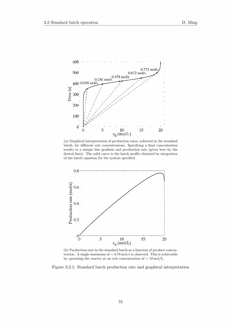
3.2 Standard batch operation D. Ming
(a) Graphical interpretation of production rates, achieved in the standardbatch, for different exit concentrations. Specifying a final concentrationresults in a unique line gradient and production rate (given here by thedotted lines). The solid curve is the batch profile obtained by integrationof the batch equation for the system specified.
(b) Production rate in the standard batch as a function of product concen-tration. A single maximum of ∼ 0.78mol/s is observed. This is achievableby operating the reactor at an exit concentration of ∼ 19mol/L.
Figure 3.2.1: Standard batch production rate and graphical interpretation
55
3.2 Standard batch operation D. Ming
overall production rate for a standard batch over multiple cycles is thus identical tothe production rate for a single batch reaction.
Figure 3.2.1a also shows the production rate for various exit conditions markedoff as coordinate points. When the two points are joined, the gradient of the straightline segment is m = �t0/
(cB − c0B
)and, according to eq 3.2.2, is proportional to the
inverse of the production rate P = Vtot/m. The rate of production is therefore atits highest when the gradient of the line is minimised.
Observation 1: Production rate can be associated with a straight line in concen-tration – time space. This value is highest when the gradient of the line isminimised.
3.2.2 Initial observations and modifications
Let us observe the effect of mixing product with feed for subsequent cycles. Thefollowing conditions will be assumed for purposes of illustration:
• The exit concentration of component B is fixed at cB = 19.0mol/L.
• The starting mixture concentration of component B is c∗B = 1.5mol/L. Bymass balance, it is found that ∼7.89 % of the product volume must be retainedin order to achieve the desired mixture concentration. The correspondingconcentration of component A is then calculated to be 18.5mol/L accordingly.The corresponding reaction time for the new initial condition is then 136 s.
The order of tasks is then as follows:
1. Run a standard batch with initial concentrations of c0A = 20mol/L and c0B =
1× 10⁻⁶ mol/L until the concentration of B is cB = 19.0mol/L. Using Figure3.2.1a or solving eq 3.2.1 directly, the reaction time for this cycle is found tobe ∼ 492 s.
2. Empty the contents of the vessel but retain 7.89% of the volume for the nextcycle. If the vessel volume is 20L, then approximately 1.578L of product isheld back; the remaining 18.422L may then be transferred as product. Since18.422L of product is transferred, 350.018mol of B is produced in the cycle.
3. Refill the vessel again to 20L with fresh feed. That is, since 1.578L of thevessel is already taken by the previous product, only 18.422L of the feed isrequired. By mass balance, the concentrations of A and B in the vessel afterfilling are then c∗A = 18.5mol/L and c∗B = 1.5mol/L, respectively.
4. Run the second cycle until the concentration of B again reaches cB = 19.0mol/L.Since the starting concentration in this cycle differs to the first, the reactiontime to reach final product is also different. Again, eq 3.2.1 can be solvedgiving a reaction time of 136 s for the second cycle.
56
3.2 Standard batch operation D. Ming
Table 3.1: Production rate with mixing after four cycles for an exit concentrationof cB = 19.0mol/L and 7.89 % of product retained for mixing. For each successivebatch, the production rate is improved. By comparison, the production rate in thestandard batch for the same exit concentration is fixed at 0.772mol/s.
Production per cycle (mol)Stages i ii iii iv Total
time(s)
Overallproduction
rate (mol/s)1 380 - - - 492 0.7722 350.018 380 - - 628 1.163 350.018 350.018 380 - 764 1.414 350.018 350.018 350.018 380 900 1.59
5. Repeat steps 2 to 4 until the desired amount of product is reached.
Table 3.1 summarises the results for four successive batches using this approach.Notice that even though the amount of product produced per cycle is less (350.018mol
for 7.89% retained, as opposed to 380mol for the full volume), the reaction timesper cycle are decreased as a result of the different starting concentration. After suf-ficiently many batches, the effect of the first and last batch on the overall productionrate is small, and hence the average production rate is influenced by the intermediatecycles, which for the specific scenario here is given by P∗ = 350.018/136mol/s. Wecan then determine the limiting production rate after many batches as that given bythe intermediate cycles. This production rate may also be represented graphicallyon the concentration profile. The final concentration is the same as that previously,however the initial point is modified to a new point on the profile, which is a functionof the retained fraction. The straight line joining these two points in c-t space thusrepresents the steady state production rate for the retained case.
The gradient of the new line is shallower than the original, which by eq 3.2.2,indicates a higher production rate. By graphical interpretation, maximising theproduction rate for a specified exit concentration on the curve indicates searchingfor the starting concentration on the profile that is associated with the straight linehaving minimal gradient.
Inasmuch as the production rate for the standard batch can be expressed interms of a line gradient, P∗ is also expressible in this manner
P∗ =Vtotm∗
where m∗ = ∆t∗/ (ci − c∗i ). The relative gain in production rate is thus also givenin terms of line gradients by (P∗/P) = (m/m∗). Thus, the results of this exampleindicate that the production rate in a standard batch may be improved by retaining
57
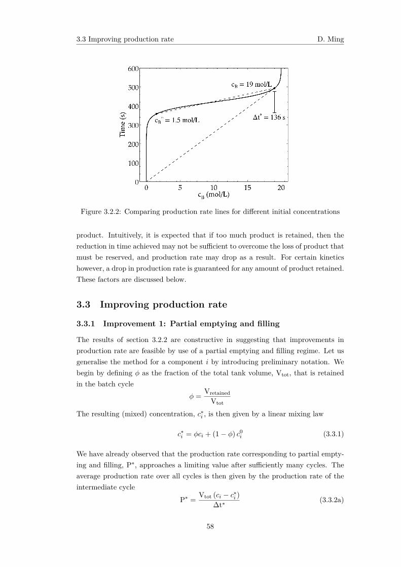
3.3 Improving production rate D. Ming
Figure 3.2.2: Comparing production rate lines for different initial concentrations
product. Intuitively, it is expected that if too much product is retained, then thereduction in time achieved may not be sufficient to overcome the loss of product thatmust be reserved, and production rate may drop as a result. For certain kineticshowever, a drop in production rate is guaranteed for any amount of product retained.These factors are discussed below.
3.3 Improving production rate
3.3.1 Improvement 1: Partial emptying and filling
The results of section 3.2.2 are constructive in suggesting that improvements inproduction rate are feasible by use of a partial emptying and filling regime. Let usgeneralise the method for a component i by introducing preliminary notation. Webegin by defining ϕ as the fraction of the total tank volume, Vtot, that is retainedin the batch cycle
ϕ =Vretained
Vtot
The resulting (mixed) concentration, c∗i , is then given by a linear mixing law
c∗i = ϕci + (1− ϕ) c0i (3.3.1)
We have already observed that the production rate corresponding to partial empty-ing and filling, P∗, approaches a limiting value after sufficiently many cycles. Theaverage production rate over all cycles is then given by the production rate of theintermediate cycle
P∗ =Vtot (ci − c∗i )
∆t∗ (3.3.2a)
58
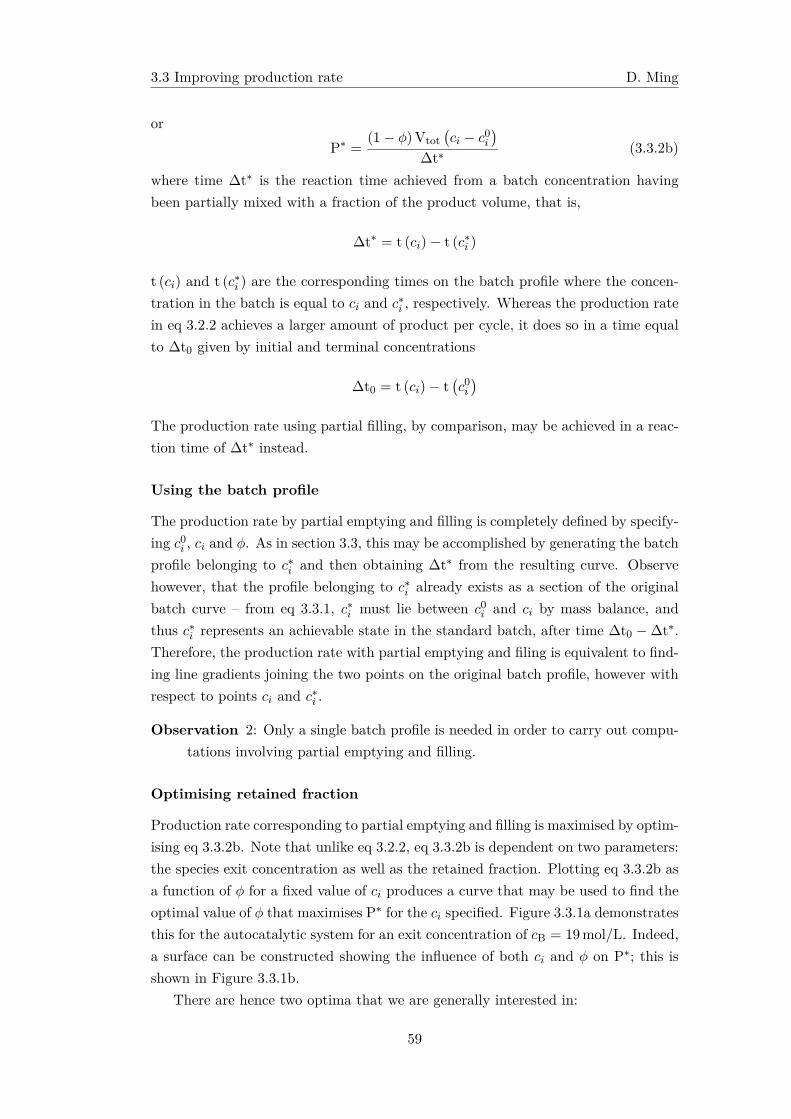
3.3 Improving production rate D. Ming
orP∗ =
(1− ϕ)Vtot(ci − c0i
)∆t∗ (3.3.2b)
where time ∆t∗ is the reaction time achieved from a batch concentration havingbeen partially mixed with a fraction of the product volume, that is,
∆t∗ = t (ci)− t (c∗i )
t (ci) and t (c∗i ) are the corresponding times on the batch profile where the concen-tration in the batch is equal to ci and c∗i , respectively. Whereas the production ratein eq 3.2.2 achieves a larger amount of product per cycle, it does so in a time equalto ∆t0 given by initial and terminal concentrations
∆t0 = t (ci)− t(c0i)
The production rate using partial filling, by comparison, may be achieved in a reac-tion time of ∆t∗ instead.
Using the batch profile
The production rate by partial emptying and filling is completely defined by specify-ing c0i , ci and ϕ. As in section 3.3, this may be accomplished by generating the batchprofile belonging to c∗i and then obtaining ∆t∗ from the resulting curve. Observehowever, that the profile belonging to c∗i already exists as a section of the originalbatch curve – from eq 3.3.1, c∗i must lie between c0i and ci by mass balance, andthus c∗i represents an achievable state in the standard batch, after time ∆t0 −∆t∗.Therefore, the production rate with partial emptying and filing is equivalent to find-ing line gradients joining the two points on the original batch profile, however withrespect to points ci and c∗i .
Observation 2: Only a single batch profile is needed in order to carry out compu-tations involving partial emptying and filling.
Optimising retained fraction
Production rate corresponding to partial emptying and filling is maximised by optim-ising eq 3.3.2b. Note that unlike eq 3.2.2, eq 3.3.2b is dependent on two parameters:the species exit concentration as well as the retained fraction. Plotting eq 3.3.2b asa function of ϕ for a fixed value of ci produces a curve that may be used to find theoptimal value of ϕ that maximises P∗ for the ci specified. Figure 3.3.1a demonstratesthis for the autocatalytic system for an exit concentration of cB = 19mol/L. Indeed,a surface can be constructed showing the influence of both ci and ϕ on P∗; this isshown in Figure 3.3.1b.
There are hence two optima that we are generally interested in:
59
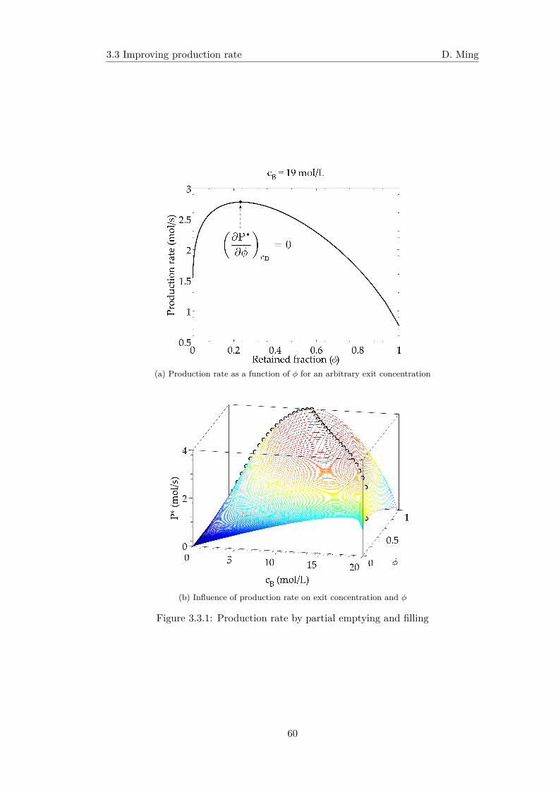
3.3 Improving production rate D. Ming
(a) Production rate as a function of ϕ for an arbitrary exit concentration
(b) Influence of production rate on exit concentration and ϕ
Figure 3.3.1: Production rate by partial emptying and filling
60
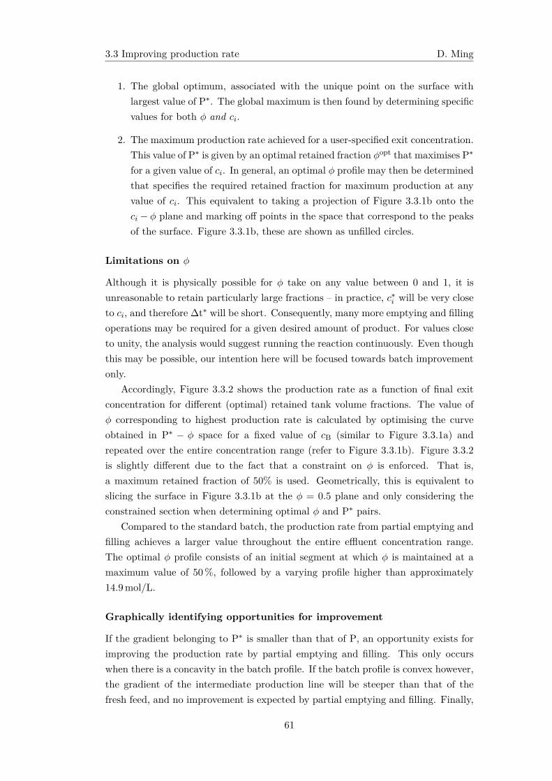
3.3 Improving production rate D. Ming
1. The global optimum, associated with the unique point on the surface withlargest value of P∗. The global maximum is then found by determining specificvalues for both ϕ and ci.
2. The maximum production rate achieved for a user-specified exit concentration.This value of P∗ is given by an optimal retained fraction ϕopt that maximises P∗
for a given value of ci. In general, an optimal ϕ profile may then be determinedthat specifies the required retained fraction for maximum production at anyvalue of ci. This equivalent to taking a projection of Figure 3.3.1b onto theci − ϕ plane and marking off points in the space that correspond to the peaksof the surface. Figure 3.3.1b, these are shown as unfilled circles.
Limitations on ϕ
Although it is physically possible for ϕ take on any value between 0 and 1, it isunreasonable to retain particularly large fractions – in practice, c∗i will be very closeto ci, and therefore ∆t∗ will be short. Consequently, many more emptying and fillingoperations may be required for a given desired amount of product. For values closeto unity, the analysis would suggest running the reaction continuously. Even thoughthis may be possible, our intention here will be focused towards batch improvementonly.
Accordingly, Figure 3.3.2 shows the production rate as a function of final exitconcentration for different (optimal) retained tank volume fractions. The value ofϕ corresponding to highest production rate is calculated by optimising the curveobtained in P∗ − ϕ space for a fixed value of cB (similar to Figure 3.3.1a) andrepeated over the entire concentration range (refer to Figure 3.3.1b). Figure 3.3.2is slightly different due to the fact that a constraint on ϕ is enforced. That is,a maximum retained fraction of 50% is used. Geometrically, this is equivalent toslicing the surface in Figure 3.3.1b at the ϕ = 0.5 plane and only considering theconstrained section when determining optimal ϕ and P∗ pairs.
Compared to the standard batch, the production rate from partial emptying andfilling achieves a larger value throughout the entire effluent concentration range.The optimal ϕ profile consists of an initial segment at which ϕ is maintained at amaximum value of 50 %, followed by a varying profile higher than approximately14.9mol/L.
Graphically identifying opportunities for improvement
If the gradient belonging to P∗ is smaller than that of P, an opportunity exists forimproving the production rate by partial emptying and filling. This only occurswhen there is a concavity in the batch profile. If the batch profile is convex however,the gradient of the intermediate production line will be steeper than that of thefresh feed, and no improvement is expected by partial emptying and filling. Finally,
61
3.3 Improving production rate D. Ming
Figure 3.3.2: Comparison of production rates for partial emptying and filling (solidline), and the standard batch (−o−); the associated optimal ϕ profile (-×-) has alsobeen plotted for bounds 0% ≤ ϕ ≤ 50%. The production rate by partial emptying issignificantly higher than what is available from the standard batch production rate(ϕ = 0.0) by the appropriate choice of ϕ value.
if the batch profile is linear, the production rate by both methods is expected to beequal, although emptying and filling may favour standard batch operation. This issummarised in Figure 3.3.3.
Observation 3: If the batch profile contains a concavity, then production rate canbe improved by partial emptying and filling.
3.3.2 Improvement 2: Improving production rates for other exitconcentrations
In addition to providing recommendations for when opportunities for improvementexist, Figure 3.3.2 also offers insight into identification of an optimal sequence ofoperation, or structure; such insight may be difficult to achieve by ordinary optim-isation methods alone. Note also that this procedure is equally applicable to thestandard batch, but we shall remain with partial emptying for illustration.
To begin, observe that a maximum production rate of ∼ 3.85mol/s is achievedby partial emptying and filling, corresponding to a 50 % retained volume fraction.Although it is clear from the graph that this production rate is obtained for adistinct (optimal) exit concentration ci, our motivation here is to show how the batchstructure may be modified to improve production rate for concentrations differentto copt
i . In particular, our approach will be to utilise the maximum production rate
62
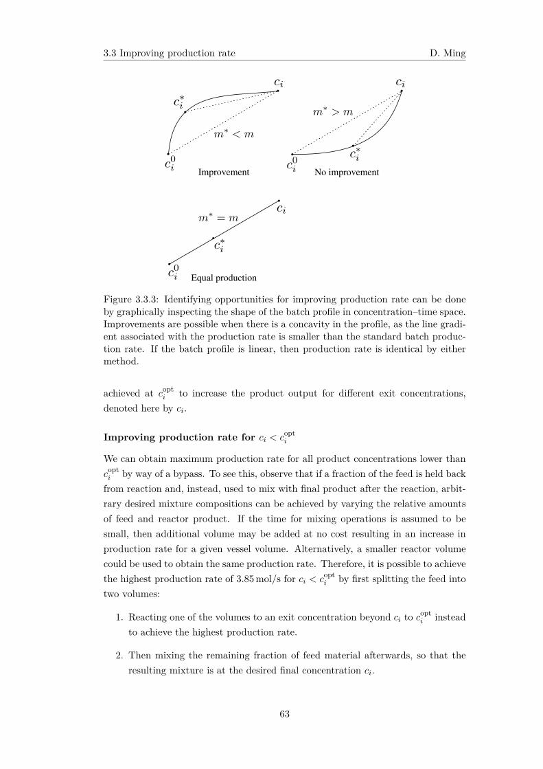
3.3 Improving production rate D. Ming
Improvement No improvement
Equal production
Figure 3.3.3: Identifying opportunities for improving production rate can be doneby graphically inspecting the shape of the batch profile in concentration–time space.Improvements are possible when there is a concavity in the profile, as the line gradi-ent associated with the production rate is smaller than the standard batch produc-tion rate. If the batch profile is linear, then production rate is identical by eithermethod.
achieved at copti to increase the product output for different exit concentrations,
denoted here by ci.
Improving production rate for ci < copti
We can obtain maximum production rate for all product concentrations lower thancopti by way of a bypass. To see this, observe that if a fraction of the feed is held back
from reaction and, instead, used to mix with final product after the reaction, arbit-rary desired mixture compositions can be achieved by varying the relative amountsof feed and reactor product. If the time for mixing operations is assumed to besmall, then additional volume may be added at no cost resulting in an increase inproduction rate for a given vessel volume. Alternatively, a smaller reactor volumecould be used to obtain the same production rate. Therefore, it is possible to achievethe highest production rate of 3.85mol/s for ci < copt
i by first splitting the feed intotwo volumes:
1. Reacting one of the volumes to an exit concentration beyond ci to copti instead
to achieve the highest production rate.
2. Then mixing the remaining fraction of feed material afterwards, so that theresulting mixture is at the desired final concentration ci.
63
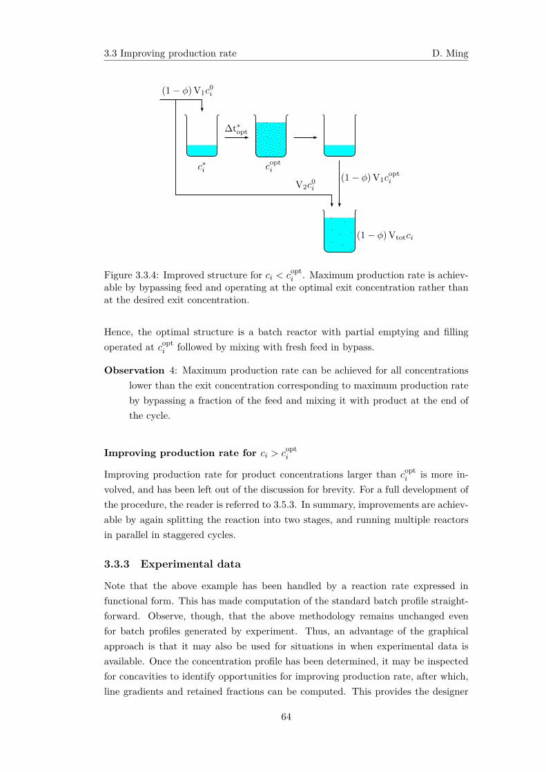
3.3 Improving production rate D. Ming
Figure 3.3.4: Improved structure for ci < copti . Maximum production rate is achiev-
able by bypassing feed and operating at the optimal exit concentration rather thanat the desired exit concentration.
Hence, the optimal structure is a batch reactor with partial emptying and fillingoperated at copt
i followed by mixing with fresh feed in bypass.
Observation 4: Maximum production rate can be achieved for all concentrationslower than the exit concentration corresponding to maximum production rateby bypassing a fraction of the feed and mixing it with product at the end ofthe cycle.
Improving production rate for ci > copti
Improving production rate for product concentrations larger than copti is more in-
volved, and has been left out of the discussion for brevity. For a full development ofthe procedure, the reader is referred to 3.5.3. In summary, improvements are achiev-able by again splitting the reaction into two stages, and running multiple reactorsin parallel in staggered cycles.
3.3.3 Experimental data
Note that the above example has been handled by a reaction rate expressed infunctional form. This has made computation of the standard batch profile straight-forward. Observe, though, that the above methodology remains unchanged evenfor batch profiles generated by experiment. Thus, an advantage of the graphicalapproach is that it may also be used for situations in when experimental data isavailable. Once the concentration profile has been determined, it may be inspectedfor concavities to identify opportunities for improving production rate, after which,line gradients and retained fractions can be computed. This provides the designer
64
3.3 Improving production rate D. Ming
quantitative information regarding the potential improvement in the system over thestandard batch without the need for a detailed model, or before a detailed modelhas been developed.
Remark
Since line gradients and optimal retained fractions are directly determined by pointson the concentration profile, the quality of the recommendations is influenced sig-nificantly by the quality of the experimentally measured data. The resulting pro-duction rate calculations may be adversely affected by ‘noisy’ data, in which suddenand steep changes in the gradient of the measured data are observed over time.In practice, when experimentally measured data are used with the method, an ap-proximating function is employed to provide smoothed approximations of the data,suitable for gradient calculations. In this work, cubic spline interpolation is usedwhen the method is operated on experimental data. Production rates and retainedfractions are then calculated based on the cubic spline interpolant of the data. Thisallows for both a slightly more smoothed data set, as well as prediction of productionrates for points that are not given at the discrete points of measurement obtainedduring experiment.
Observation 5: Calculations can be performed in the absence of a detailed modelsince only points from the batch profile are required.
A note should be made regarding the production of undesired products. If we runthe reactor at conditions that are optimal for the production rate of the desiredcomponent, then we may also incur the risk of overproducing undesired species aswell. In this case, there may be benefit to measuring the concentrations of bothspecies so that two separate batch profiles can be obtained. It is easy then tocompute production rates for both species to determine the best compromise betweenthe two. Bypassing feed may also give a more favourable concentration in undesiredcomponents if we can afford to run the reactor at lower product concentrations.Nevertheless, it may be more practical to change operating variables such as theoperating temperature to control the reactions for example. Again, benefit may befound from using these methods as a simple method of improving the production ratefor a specific purity constraint, and then using traditional optimisation for furtherimprovement.
3.3.4 Method
In order to generate the optimal P∗ and ϕ profiles in Figure 3.3.2, the followingprocedure is followed:
1. Generate the concentration profile (concentration versus time plot) for thespecies of interest. This may be achieved with a kinetic model by integrat-
65
3.4 Examples D. Ming
ing the batch equation using the available reaction kinetics. Otherwise, theconcentration profile is obtained from experimentally measured data.
2. For each concentration ci in the measured concentration range, an optimalvalue of ϕ exists that maximises P∗. In order to find the optimal value of ϕ,a curve, such as that given in Figure 3.3.1a, must be optimised for each valueof ci:
(a) This is achieved by performing a constrained optimisation – maximisingeq 3.3.2b for the value of ci specified, bounded by 0 ≤ ϕ ≤ ϕmax, whereϕmax is the maximum allowed retained fraction per cycle. If a stand-ardised optimisation routine is employed for the optimisation, then in-terpolation may be required. In general, we aim to find the ϕ profilecorresponding to following condition(
∂P∗
∂ϕ
)ci
= 0
where P∗ is given by eq 3.3.2b. The value of ∆t∗ used in eq 3.3.2b isdetermined by interpolating the concentration profile to find t (ci) andt (c∗i ).
(b) Record the value of ϕ and P∗ obtained from the optimisation.
3. Repeat step 2 until all points in the concentration profile have been calculated.The set of ϕ’s and P∗’s corresponding to each value of ci on the concentrationprofile are thus the optimal retained fraction and partial emptying productionrate, respectively.
The procedure described above only requires concentration and time data and iseasily programmed on a computer as a compact function. Optimisations requiredin point 2(a) above may still be carried out numerically with experimental data ifinterpolation of the data (with a suitable interpolating function) is used.
3.4 Examples
3.4.1 Hydrolysis of propylene oxide
The production of propylene glycol is produced by the hydrolysis of propylene oxidein the following reaction (Fogler, 2006)
CH2OCHCH3 + H2O → CH2OCHOHCH3
A + D → B
66
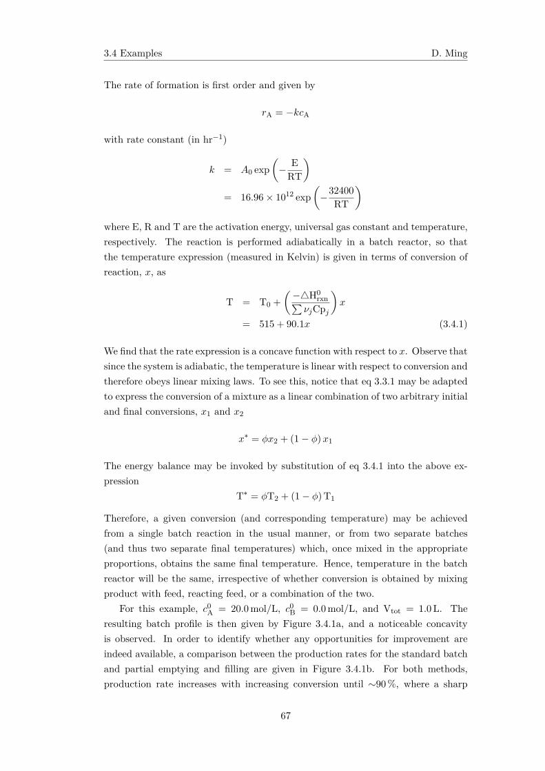
3.4 Examples D. Ming
The rate of formation is first order and given by
rA = −kcA
with rate constant (in hr−1)
k = A0 exp(− E
RT
)= 16.96× 10¹² exp
(−32400
RT
)where E, R and T are the activation energy, universal gas constant and temperature,respectively. The reaction is performed adiabatically in a batch reactor, so thatthe temperature expression (measured in Kelvin) is given in terms of conversion ofreaction, x, as
T = T0 +
(−△H0
rxn∑νjCpj
)x
= 515 + 90.1x (3.4.1)
We find that the rate expression is a concave function with respect to x. Observe thatsince the system is adiabatic, the temperature is linear with respect to conversion andtherefore obeys linear mixing laws. To see this, notice that eq 3.3.1 may be adaptedto express the conversion of a mixture as a linear combination of two arbitrary initialand final conversions, x1 and x2
x∗ = ϕx2 + (1− ϕ)x1
The energy balance may be invoked by substitution of eq 3.4.1 into the above ex-pression
T∗ = ϕT2 + (1− ϕ)T1
Therefore, a given conversion (and corresponding temperature) may be achievedfrom a single batch reaction in the usual manner, or from two separate batches(and thus two separate final temperatures) which, once mixed in the appropriateproportions, obtains the same final temperature. Hence, temperature in the batchreactor will be the same, irrespective of whether conversion is obtained by mixingproduct with feed, reacting feed, or a combination of the two.
For this example, c0A = 20.0mol/L, c0B = 0.0mol/L, and Vtot = 1.0L. Theresulting batch profile is then given by Figure 3.4.1a, and a noticeable concavityis observed. In order to identify whether any opportunities for improvement areindeed available, a comparison between the production rates for the standard batchand partial emptying and filling are given in Figure 3.4.1b. For both methods,production rate increases with increasing conversion until ∼90 %, where a sharp
67
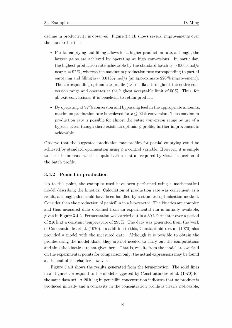
3.4 Examples D. Ming
decline in productivity is observed. Figure 3.4.1b shows several improvements overthe standard batch:
• Partial emptying and filling allows for a higher production rate, although, thelargest gains are achieved by operating at high conversions. In particular,the highest production rate achievable by the standard batch is ∼ 0.006mol/snear x = 92%, whereas the maximum production rate corresponding to partialemptying and filling is ∼ 0.01367mol/s (an approximate 220 % improvement).The corresponding optimum ϕ profile (-×-) is flat throughout the entire con-version range and operates at the highest acceptable limit of 50 %. Thus, forall exit conversions, it is beneficial to retain product.
• By operating at 92 % conversion and bypassing feed in the appropriate amounts,maximum production rate is achieved for x ≤ 92% conversion. Thus maximumproduction rate is possible for almost the entire conversion range by use of abypass. Even though there exists an optimal ϕ profile, further improvement isachievable.
Observe that the suggested production rate profiles for partial emptying could beachieved by standard optimisation using ϕ a control variable. However, it is simpleto check beforehand whether optimisation is at all required by visual inspection ofthe batch profile.
3.4.2 Penicillin production
Up to this point, the examples used have been performed using a mathematicalmodel describing the kinetics. Calculation of production rate was convenient as aresult, although, this could have been handled by a standard optimisation method.Consider then the production of penicillin in a bio-reactor. The kinetics are complexand thus measured data obtained from an experimental run is initially available,given in Figure 3.4.2. Fermentation was carried out in a 30L fermenter over a periodof 216h at a constant temperature of 295K. The data was generated from the workof Constantinides et al. (1970). In addition to this, Constantinides et al. (1970) alsoprovided a model with the measured data. Although it is possible to obtain theprofiles using the model alone, they are not needed to carry out the computationsand thus the kinetics are not given here. That is, results from the model are overlaidon the experimental points for comparison only; the actual expressions may be foundat the end of the chapter however.
Figure 3.4.3 shows the results generated from the fermentation. The solid linesin all figures correspond to the model suggested by Constantinides et al. (1970) forthe same data set. A 20 h lag in penicillin concentration indicates that no product isproduced initially and a concavity in the concentration profile is clearly noticeable,
68
3.4 Examples D. Ming
(a) Batch profile for the hydrolysis of propylene oxide.
(b) Production rate comparison for propylene oxide. The production rateby partial emptying (black solid line) may be improved significantly for allconversions by operating at the maximum retained volume fraction, seenhere by the constant optimum ϕ profile (-×-). The gain in production rateby mixing over the standard batch increases with higher conversions.
Figure 3.4.1: Hydrolysis of propylene oxide.
69
3.4 Examples D. Ming
Figure 3.4.2: Concentration profile for penicillin production. No penicillin is pro-duced in the first 20 h of operation.
although there is in fact a small, approximately linear section, up to 0.03 g/L. Dueto the concavity, production rate is expected to be improved by retaining product.
The data were therefore used to compute the production rates of both the stand-ard batch and partial emptying and filling; this is given in Figure 3.4.3a. Throughoutthe entire concentration range, the production rate by partial emptying is larger thanthe standard batch. In particular, this value is ∼ 8.7mg/h at maximum productionrate compared to ∼ 6.0mg/h for the standard batch. The corresponding retainedfractions generated using the experimental points are also shown in Figure 3.4.3b.As discussed above, there is a small linear section in the profile near the start andthus the optimum ϕ profile initially shows a section where no product is retained.For exit concentrations less than approximately 7 g/L, the profile is flat. This sug-gests that production rate is maximised by retaining as much product as possible.For product concentrations beyond this value, the optimum retained fraction followsa varying profile that steadily decreases to 0 %. Again, the curve calculated fromthe rate expressions is fairly close to the experimental points. Partial emptying andfilling allows one to eliminate the initial 20h lag phase, and thus production rate islarger when compared to the standard batch. For this reason, it is recommendedthat at least trace amounts of product be retained.
It is interesting to note that these recommendations are what are done in prac-tice. It is common in biological reactions to recycle a fraction of cells from theproduct to allow sufficient time for cells to reproduce, and to minimise washout(Crueger and Crueger, 1984). Fed-batch operation is also a common method of im-proving production rate in practice and could be used to achieve an intermediateconcentration within the batch. In this regard, the results of the graphical analysis
70
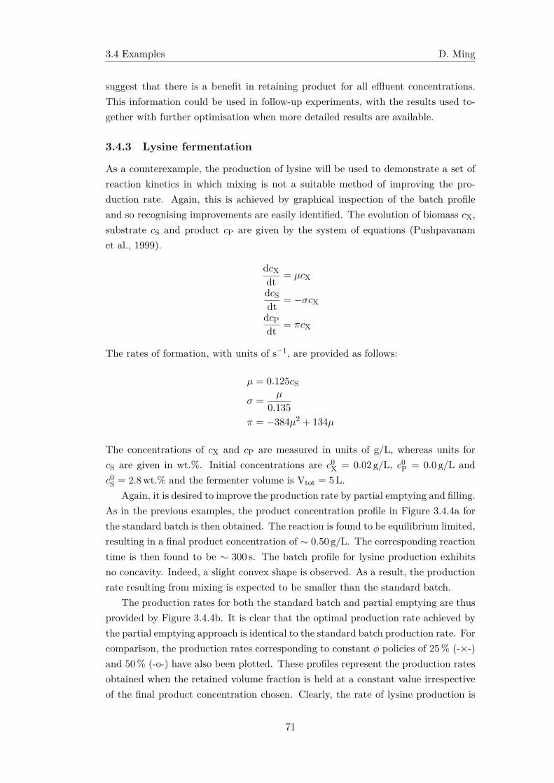
3.4 Examples D. Ming
suggest that there is a benefit in retaining product for all effluent concentrations.This information could be used in follow-up experiments, with the results used to-gether with further optimisation when more detailed results are available.
3.4.3 Lysine fermentation
As a counterexample, the production of lysine will be used to demonstrate a set ofreaction kinetics in which mixing is not a suitable method of improving the pro-duction rate. Again, this is achieved by graphical inspection of the batch profileand so recognising improvements are easily identified. The evolution of biomass cX,substrate cS and product cP are given by the system of equations (Pushpavanamet al., 1999).
dcXdt = µcX
dcSdt = −σcX
dcPdt = πcX
The rates of formation, with units of s−1, are provided as follows:
µ = 0.125cS
σ =µ
0.135
π = −384µ2 + 134µ
The concentrations of cX and cP are measured in units of g/L, whereas units forcS are given in wt.%. Initial concentrations are c0X = 0.02 g/L, c0P = 0.0 g/L andc0S = 2.8wt.% and the fermenter volume is Vtot = 5L.
Again, it is desired to improve the production rate by partial emptying and filling.As in the previous examples, the product concentration profile in Figure 3.4.4a forthe standard batch is then obtained. The reaction is found to be equilibrium limited,resulting in a final product concentration of ∼ 0.50 g/L. The corresponding reactiontime is then found to be ∼ 300 s. The batch profile for lysine production exhibitsno concavity. Indeed, a slight convex shape is observed. As a result, the productionrate resulting from mixing is expected to be smaller than the standard batch.
The production rates for both the standard batch and partial emptying are thusprovided by Figure 3.4.4b. It is clear that the optimal production rate achieved bythe partial emptying approach is identical to the standard batch production rate. Forcomparison, the production rates corresponding to constant ϕ policies of 25 % (-×-)and 50 % (-o-) have also been plotted. These profiles represent the production ratesobtained when the retained volume fraction is held at a constant value irrespectiveof the final product concentration chosen. Clearly, the rate of lysine production is
71
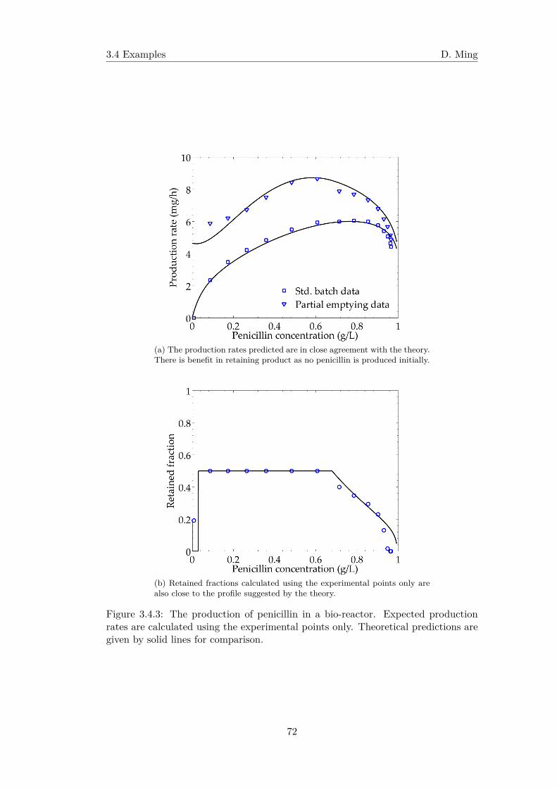
3.4 Examples D. Ming
(a) The production rates predicted are in close agreement with the theory.There is benefit in retaining product as no penicillin is produced initially.
(b) Retained fractions calculated using the experimental points only arealso close to the profile suggested by the theory.
Figure 3.4.3: The production of penicillin in a bio-reactor. Expected productionrates are calculated using the experimental points only. Theoretical predictions aregiven by solid lines for comparison.
72
3.5 Further remarks D. Ming
reduced for increasing retained volume fractions and hence for 0% ≤ ϕ ≤ 100%, thecorresponding production rate by partial emptying is smaller than a standard batch.
It follows that there exists no opportunity for improvement by mixing for thesekinetics. Although no improvement is possible, the graphical approach has stillprovided insight into an optimal operating policy. This is still useful in itself. ϕ = 0%
3.5 Further remarks
3.5.1 Transfer time
The contribution of emptying and filling times, or transfer time, may be accountedfor by the addition of extra terms in the production rate equations. In general, thisquantity must be added to each cycle, and as a result, may be regarded as constant.The production rate equations are then adapted as follows
P =Vtot
(ci − c0i
)(�t0 + tT)
P∗ =(1− ϕ)Vtot (ci − c∗i )(
�t∗ + t∗T)
Where tT denotes transfer time. Here, use of the overbar signals that productionrate under consideration of transfer time has been accounted for. Two observationscan be made with respect to its inclusion:
1. Clearly, tT serves to increase the gradients of the production lines, suggestinga decrease in production rate.
2. Since tT is associated with an emptying and filling rate, given here by r,transfer time is a function of the volume transferred, and by association, ϕ.As a result, the transfer time for partial emptying and filling is smaller thanthe standard batch. The ratio of the production rates defined above can bewritten in terms of filling rate and retained fraction as follows
P∗
P=
(P∗
P
)ξ (3.5.1)
whereξ =
[r
Vtot+
1
∆t0
]/
[r
Vtot+
(1− ϕ)
∆t∗
](3.5.2)
The derivation of eq 3.5.1 can be found in appendix A.1. The relative gainin production efficiency can be viewed as the product of two factors: a stand-ard ratio of production performance where no allowance for transfer time isaccounted for, multiplied by a transfer time factor. Due to the dependence onϕ, this factor is approximately equal to unity. The relative gain in productionrate therefore might not be significantly influenced by transfer time. Figure3.5.1 provides a plot of this ratio for different filling rates.
73
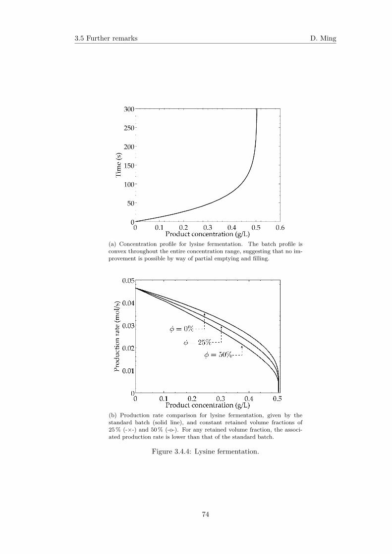
3.5 Further remarks D. Ming
(a) Concentration profile for lysine fermentation. The batch profile isconvex throughout the entire concentration range, suggesting that no im-provement is possible by way of partial emptying and filling.
(b) Production rate comparison for lysine fermentation, given by thestandard batch (solid line), and constant retained volume fractions of25 % (-×-) and 50 % (-o-). For any retained volume fraction, the associ-ated production rate is lower than that of the standard batch.
Figure 3.4.4: Lysine fermentation.
74
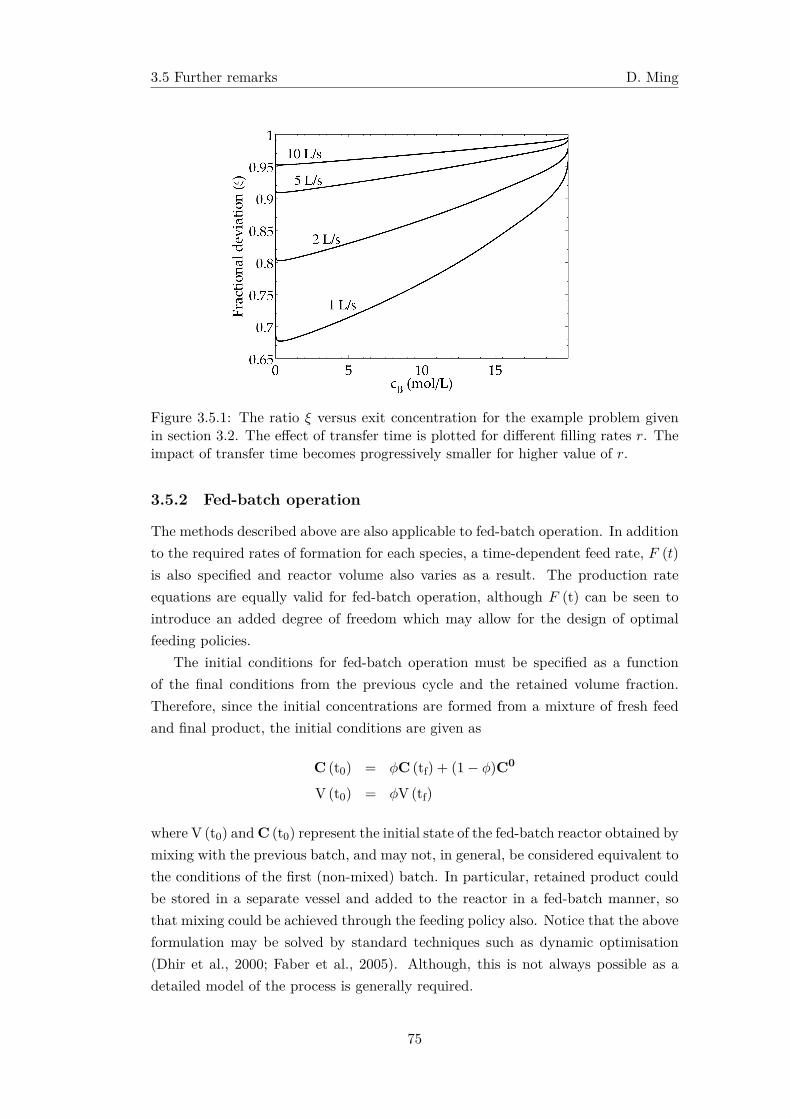
3.5 Further remarks D. Ming
Figure 3.5.1: The ratio ξ versus exit concentration for the example problem givenin section 3.2. The effect of transfer time is plotted for different filling rates r. Theimpact of transfer time becomes progressively smaller for higher value of r.
3.5.2 Fed-batch operation
The methods described above are also applicable to fed-batch operation. In additionto the required rates of formation for each species, a time-dependent feed rate, F (t)
is also specified and reactor volume also varies as a result. The production rateequations are equally valid for fed-batch operation, although F (t) can be seen tointroduce an added degree of freedom which may allow for the design of optimalfeeding policies.
The initial conditions for fed-batch operation must be specified as a functionof the final conditions from the previous cycle and the retained volume fraction.Therefore, since the initial concentrations are formed from a mixture of fresh feedand final product, the initial conditions are given as
C (t0) = ϕC (tf) + (1− ϕ)C0
V (t0) = ϕV (tf)
where V (t0) and C (t0) represent the initial state of the fed-batch reactor obtained bymixing with the previous batch, and may not, in general, be considered equivalent tothe conditions of the first (non-mixed) batch. In particular, retained product couldbe stored in a separate vessel and added to the reactor in a fed-batch manner, sothat mixing could be achieved through the feeding policy also. Notice that the aboveformulation may be solved by standard techniques such as dynamic optimisation(Dhir et al., 2000; Faber et al., 2005). Although, this is not always possible as adetailed model of the process is generally required.
75
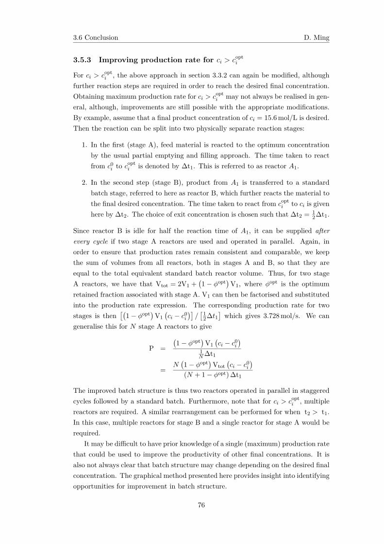
3.6 Conclusion D. Ming
3.5.3 Improving production rate for ci > copti
For ci > copti , the above approach in section 3.3.2 can again be modified, although
further reaction steps are required in order to reach the desired final concentration.Obtaining maximum production rate for ci > copt
i may not always be realised in gen-eral, although, improvements are still possible with the appropriate modifications.By example, assume that a final product concentration of ci = 15.6mol/L is desired.Then the reaction can be split into two physically separate reaction stages:
1. In the first (stage A), feed material is reacted to the optimum concentrationby the usual partial emptying and filling approach. The time taken to reactfrom c0
i to copti is denoted by ∆t1. This is referred to as reactor A1.
2. In the second step (stage B), product from A1 is transferred to a standardbatch stage, referred to here as reactor B, which further reacts the material tothe final desired concentration. The time taken to react from copt
i to ci is givenhere by ∆t2. The choice of exit concentration is chosen such that ∆t2 = 1
2∆t1.
Since reactor B is idle for half the reaction time of A1, it can be supplied afterevery cycle if two stage A reactors are used and operated in parallel. Again, inorder to ensure that production rates remain consistent and comparable, we keepthe sum of volumes from all reactors, both in stages A and B, so that they areequal to the total equivalent standard batch reactor volume. Thus, for two stageA reactors, we have that Vtot = 2V1 +
(1 − ϕopt)V1, where ϕopt is the optimum
retained fraction associated with stage A. V1 can then be factorised and substitutedinto the production rate expression. The corresponding production rate for twostages is then
[(1− ϕopt)V1
(ci − c0i
)]/[12∆t1
]which gives 3.728mol/s. We can
generalise this for N stage A reactors to give
P =
(1− ϕopt)V1
(ci − c0i
)1N∆t1
=N
(1− ϕopt)Vtot
(ci − c0i
)(N + 1− ϕopt)∆t1
The improved batch structure is thus two reactors operated in parallel in staggeredcycles followed by a standard batch. Furthermore, note that for ci > copt
i , multiplereactors are required. A similar rearrangement can be performed for when �t2 > �t1.In this case, multiple reactors for stage B and a single reactor for stage A would berequired.
It may be difficult to have prior knowledge of a single (maximum) production ratethat could be used to improve the productivity of other final concentrations. It isalso not always clear that batch structure may change depending on the desired finalconcentration. The graphical method presented here provides insight into identifyingopportunities for improvement in batch structure.
76
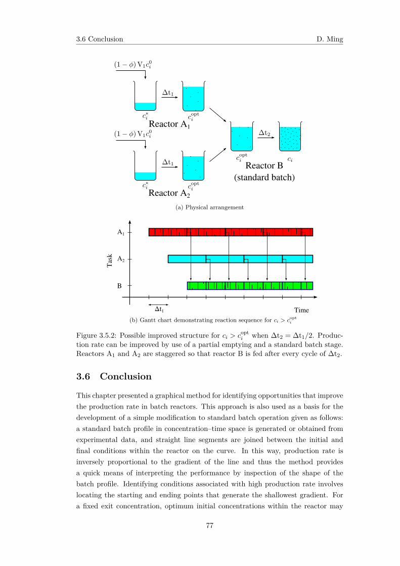
3.6 Conclusion D. Ming
Reactor A1
Reactor A2
Reactor B(standard batch)
(a) Physical arrangement
A1
A2
B
Time
Task
Δt1
(b) Gantt chart demonstrating reaction sequence for ci > copti
Figure 3.5.2: Possible improved structure for ci > copti when ∆t2 = ∆t1/2. Produc-
tion rate can be improved by use of a partial emptying and a standard batch stage.Reactors A1 and A2 are staggered so that reactor B is fed after every cycle of ∆t2.
3.6 Conclusion
This chapter presented a graphical method for identifying opportunities that improvethe production rate in batch reactors. This approach is also used as a basis for thedevelopment of a simple modification to standard batch operation given as follows:a standard batch profile in concentration–time space is generated or obtained fromexperimental data, and straight line segments are joined between the initial andfinal conditions within the reactor on the curve. In this way, production rate isinversely proportional to the gradient of the line and thus the method providesa quick means of interpreting the performance by inspection of the shape of thebatch profile. Identifying conditions associated with high production rate involveslocating the starting and ending points that generate the shallowest gradient. Fora fixed exit concentration, optimum initial concentrations within the reactor may
77
3.6 Conclusion D. Ming
be determined by locating the point associated with smallest slope. This suggeststhat the standard batch cycle can be improved by changing the initial conditionsto produce more favourable gradients. It also follows that production rate canbe improved when the batch profile contains concavities, and hence it is easy todetermine these opportunities by graphical inspection.
From this, it can be shown that instead of withdrawing the full product volumefrom the reactor at the end of each cycle, it is potentially more advantageous to re-tain a fraction of the product volume and mix with fresh feed in the following cycle.This may appear to be counter-intuitive to the normal method of batch operation.The graphical approach also provides a better understanding into identification ofimproved batch structures. In particular, the batch procedure may change depend-ing on the desired final product concentration. For all concentrations less thanthe optimal concentration, maximum production rate is achievable by bypassing afraction of the feed and mixing afterwards. For concentrations greater than theoptimum, further improvements may be achieved by distributing feed over multiplereactors operating in parallel in staggered cycles.
Several industrial examples were demonstrated to improve over the standardbatch when concavities in the batch profile were observed. For lysine productionhowever, no improvement was achieved. Inasmuch as these cases have not shown anyenhancement in production efficiency, the graphical approach still provides relevantinformation regarding the nature of the kinetics, and therefore allows for screeningof potentially productive batch structures before more complex optimisations areundertaken. Subsequent optimisation may also be easier if an appropriate structureis used in the optimisation model.
Consideration of how the production rate equations may be further applied fornon-standard batch operation was also briefly discussed. The method is equallyvalid for fed-batch operation and no alteration to the equations is required. Fur-thermore, the added flexibility of fed-batch operation provides opportunities to tailorproduction performance by variation of the feed policy.
The graphical methods described here are simple enough that they may be per-formed by those who do not have the required knowledge or resources to carry outtraditional optimisations. Additionally, this approach may also be used as a short-cut method before more sophisticated techniques are employed. Considering thatthe method only requires data points from the batch profile before meaningful in-formation can be obtained, it is possible to use these methods on experimental datain the absence of a detailed model, or before a model has been developed. Althoughthis could be viewed as an optimisation of the initial condition with splitting andmixing constraints, identifying these opportunities are not always apparent from theequations alone. The ideas presented here have come about from an understandingthat structure is an important component to the overall performance of a system.The need for simple graphical methods is therefore incredibly useful, even in modern
78
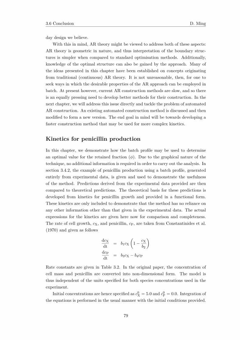
3.6 Conclusion D. Ming
day design we believe.With this in mind, AR theory might be viewed to address both of these aspects:
AR theory is geometric in nature, and thus interpretation of the boundary struc-tures is simpler when compared to standard optimisation methods. Additionally,knowledge of the optimal structure can also be gained by the approach. Many ofthe ideas presented in this chapter have been established on concepts originatingfrom traditional (continuous) AR theory. It is not unreasonable, then, for one toseek ways in which the desirable properties of the AR approach can be employed inbatch. At present however, current AR construction methods are slow, and so thereis an equally pressing need to develop better methods for their construction. In thenext chapter, we will address this issue directly and tackle the problem of automatedAR construction. An existing automated construction method is discussed and thenmodified to form a new version. The end goal in mind will be towards developing afaster construction method that may be used for more complex kinetics.
Kinetics for penicillin production
In this chapter, we demonstrate how the batch profile may be used to determinean optimal value for the retained fraction (ϕ). Due to the graphical nature of thetechnique, no additional information is required in order to carry out the analysis. Insection 3.4.2, the example of penicillin production using a batch profile, generatedentirely from experimental data, is given and used to demonstrate the usefulnessof the method. Predictions derived from the experimental data provided are thencompared to theoretical predictions. The theoretical basis for these predictions isdeveloped from kinetics for penicillin growth and provided in a functional form.These kinetics are only included to demonstrate that the method has no reliance onany other information other than that given in the experimental data. The actualexpressions for the kinetics are given here now for comparison and completeness.The rate of cell growth, cX, and penicillin, cP, are taken from Constantinides et al.(1970) and given as follows
dcXdt = b1cX
(1− cX
b2
)dcPdt = b3cX − b4cP
Rate constants are given in Table 3.2. In the original paper, the concentration ofcell mass and penicillin are converted into non-dimensional form. The model isthus independent of the units specified for both species concentrations used in theexperiment.
Initial concentrations are hence specified as c0X = 5.0 and c0P = 0.0. Integration ofthe equations is performed in the usual manner with the initial conditions provided.
79
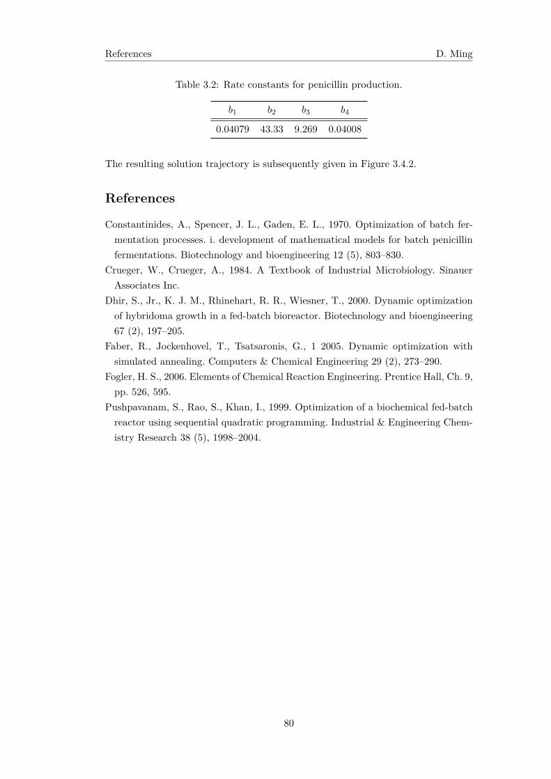
References D. Ming
Table 3.2: Rate constants for penicillin production.
b1 b2 b3 b4
0.04079 43.33 9.269 0.04008
The resulting solution trajectory is subsequently given in Figure 3.4.2.
References
Constantinides, A., Spencer, J. L., Gaden, E. L., 1970. Optimization of batch fer-mentation processes. i. development of mathematical models for batch penicillinfermentations. Biotechnology and bioengineering 12 (5), 803–830.
Crueger, W., Crueger, A., 1984. A Textbook of Industrial Microbiology. SinauerAssociates Inc.
Dhir, S., Jr., K. J. M., Rhinehart, R. R., Wiesner, T., 2000. Dynamic optimizationof hybridoma growth in a fed-batch bioreactor. Biotechnology and bioengineering67 (2), 197–205.
Faber, R., Jockenhovel, T., Tsatsaronis, G., 1 2005. Dynamic optimization withsimulated annealing. Computers & Chemical Engineering 29 (2), 273–290.
Fogler, H. S., 2006. Elements of Chemical Reaction Engineering. Prentice Hall, Ch. 9,pp. 526, 595.
Pushpavanam, S., Rao, S., Khan, I., 1999. Optimization of a biochemical fed-batchreactor using sequential quadratic programming. Industrial & Engineering Chem-istry Research 38 (5), 1998–2004.
80
Chapter 4
AR construction using rotatedbounding hyperplanes
The following chapter has been adapted from published work with permission. Theassociated paper is (Ming, D., Hildebrandt, D., Glasser, D., 2010. A revised methodof attainable region construction utilizing rotated bounding hyperplanes. Ind. Eng.Chem. Res. 49, 10549–10557.) Copyright (2010) American Chemical Society. D.Ming (the present author) compiled the manuscript and contributed to the ideas inthis work. D. Hildebrandt and D. Glasser supervised this work.
4.1 Introduction
For the past three decades, knowledge of the Attainable Region (AR) has allowedone to approach the problem of optimal reactor network design from a geometricviewpoint. Originally introduced by F.J.M Horn in 1967 (Horn, 1964) but laterpioneered by the work of Glasser et al. (1987), Hildebrandt (1989) and Hildebrandtand Glasser (1990), Feinberg and Hildebrandt (1997) and Feinberg (2000b,a), theAR has addressed the problem of optimal reactor design by determining all possibleoutputs for a given set of feed conditions, reaction kinetics and operating constraints.In doing so, the AR approach has allowed for the solution of a large variety of reactornetwork synthesis and optimisation problems.
In chapter 2, we discuss how many of the most recent developments in the fieldhave focused toward the advancement of algorithms for the automatic constructionof candidate ARs. Current methods of construction fall into two categories:
1. Methods which attempt to generate the AR from a known starting feed condi-tion and grow the region outwards (Rooney et al., 2000; Kauchali et al., 2002;Seodigeng et al., 2009), referred to as inside-out methods.
2. Methods that compute an initial (and possibly large) superset in which theAR is known to reside, and then progressively shrink the region inwards (Burri
81
4.2 Mathematical preliminaries D. Ming
et al., 2002; Manousiouthakis et al., 2004; Abraham and Feinberg, 2004), re-ferred to here as outside-in methods.
In this chapter, we shall be concerned with a variation of an existing outside-inalgorithm originally developed by Abraham and Feinberg (Abraham and Feinberg,2004). This procedure constructs candidate regions using a large number of bound-ing hyperplanes. Our chief objective will be to first present the necessary changesmade to the original method, and then demonstrate its application to problems inconcentration and concentration-time space, particularly in R2. We aim to showthat by a change in hyperplane placement, AR construction efficiency may be im-proved by a significant margin. We shall only be concerned with the construction ofcandidate ARs in which density and, unless specified otherwise, temperature maybe assumed constant. As in chapter 2, this allows us to assert special geometriccharacteristics of the process of mixing and hence the shape of the AR boundary.
Sections 4.2.1 to 4.2.6 provide the necessary mathematical background and gen-eral results required for the proper understanding of the modified algorithm. Sec-tions 4.3.1 and 4.3.2 introduce the reader to the original and modified constructionmethods respectively. The main motivations for improvement are also discussedat the end of section 4.3.2. Section 4.4 provides several examples for classical iso-thermal problems as well as non-standard problems that have not been implementedby the original bounding hyperplanes algorithm. These examples allow for the de-termination of the AR for a wider variety of systems and kinetics. Section 4.4.1,in particular, provides a comparison between the two approaches. Finally, section4.6 provides several remarks regarding higher dimensional constructions before con-cluding remarks are supplied in section 4.7.
4.2 Mathematical preliminaries
In chapter 2, an overview of the geometric nature of concentration and mixing isprovided. These properties are then used to define the AR by exploiting the convexnature of mixing in conjunction with the use of three fundamental reactor types.The AR construction algorithm outlined next relies on a basic understanding ofhyperplanes, as well as the geometric constituents (facets, edges, vertices) that areformed when multiple hyperplanes are arranged in space to form a convex polytope.Definitions and brief descriptions for these are also given below.
4.2.1 Hyperplanes
A hyperplane H (n,C0) is defined as one that obeys the following equation
H (n,C0) ={
C ∈ Rn : nT (C − C0) = 0}
(4.2.1)
82
4.2 Mathematical preliminaries D. Ming
where vectors C and C0 are points lying in H (n,C0) and where n is a vectororthogonal to (C − C0). A hyperplane separates a space Rn into two half-spaces.The positive and negative closed half spaces are defined by
H≥ ={
C ∈ Rn : nT (C − C0) ≥ 0}
H≤ ={
C ∈ Rn : nT (C − C0) ≤ 0} (4.2.2)
and similarly for the open half spaces
H> ={
C ∈ Rn : nT (C − C0) > 0}
H< ={
C ∈ Rn : nT (C − C0) < 0} (4.2.3)
Clearly, n forms an orthogonal subspace to H (n,C0) and may be used as a test fortangency to the plane.
4.2.2 Orthogonal and tangent vectors
The inner product of two vectors x, y may be defined by the following relation
xTy = ∥x∥ ∥y∥ cos (θ)
where θ is the angle between x and y. This relation may be used to signal when thetwo vectors are orthogonal (cos (θ) = 0) or tangent (|cos (θ)| = 1) to one another.Hence, x and y are orthogonal, if there is at least one non-zero element in x and yand where
xTy = 0 (4.2.4)
where 0 is the zero vector. Similarly, x and y are tangent if
xTy = ∥x∥ ∥y∥ (4.2.5)
where ∥x∥ and ∥y∥ represent the magnitudes of x and y, respectively. If x and yare unit vectors, then the above reduces to
xTy = 1
4.2.3 Extreme points
A point x ∈ Rn is an extreme point if it is a vertex of the convex hull. Extremepoints may not lie in the interior of the convex hull, nor in the interior of the linesegment bounding the facets of the convex polytope.
83
4.2 Mathematical preliminaries D. Ming
4.2.4 Facets and edges
A hyperplane is said to a n-face or n-facet of the convex polytope conv(P ), if n
linearly independent points in P lie on H (n,C0). An n-edge of the convex polytopeconv(P ) is one which contains n − 1 linearly independent points that make up then-face (Chand and Kapur, 1970).
4.2.5 Vertex and facet enumeration
A convex polyhedron P in Rn may be described independently both in terms of itsvertices, and in terms of its facets. P is said to be given in the vertex representation(the V-representation), when the polytope is described in terms of a collection ofvertices. Similarly, the same polyhedron is said to given in the hyperplane repres-entation (the H-representation) when the polytope is described by a collection ofhyperplane constraints of the following form:
Ax ≥ b
Notice that imposing non-negativity constraints on the component concentrationsis equivalent to expressing the system in the above form. The vertex enumerationproblem constitutes finding the vertices (corners) of P when P is described by theH-representation. Conversely, the facet enumeration problem arises when P is de-scribed by the V-representation and we wish to determine the associated hyperplaneconstraints in H-representation. We have already encountered the facet enumerationproblem on numerous occasions, disguised under the form of the convex hull of aset of points. Vertex and facet enumeration are, in the sense of convex optimiz-ation, dual problems. Solution of the one automatically results in solution of theother. It is clear that computing the convex hull of a set of points is equivalent tosolving the facet enumeration problem for a given convex polytope describing a setof achievable states in state space. Similarly, computing the extreme points of thestoichiometric subspace is equivalent to finding the intersection points that producefeasible vertices from a system of inequality constraints; we are in fact solving thevertex enumeration problem. Figure 4.2.1 gives a visual representation of the twoproblems.
4.2.6 Stoichiometric constraints
Given a system of chemical reactions and associated kinetics and feed point, weaim to determine the limits to which a given concentration may be achieved bystoichiometry alone. Knowledge of an upper bound on attainability allows one toestablish that the AR will lie in a smaller subspace in Rn (Feinberg, 2000b). Clearly,non-negativity constraints restrict the subspace to lie within the positive orthant inRn. From chapter 2, it is simple to show that tighter bounds on attainability may be
84
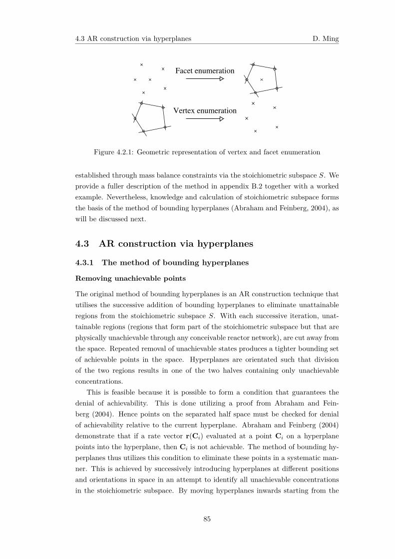
4.3 AR construction via hyperplanes D. Ming
Figure 4.2.1: Geometric representation of vertex and facet enumeration
established through mass balance constraints via the stoichiometric subspace S. Weprovide a fuller description of the method in appendix B.2 together with a workedexample. Nevertheless, knowledge and calculation of stoichiometric subspace formsthe basis of the method of bounding hyperplanes (Abraham and Feinberg, 2004), aswill be discussed next.
4.3 AR construction via hyperplanes
4.3.1 The method of bounding hyperplanes
Removing unachievable points
The original method of bounding hyperplanes is an AR construction technique thatutilises the successive addition of bounding hyperplanes to eliminate unattainableregions from the stoichiometric subspace S. With each successive iteration, unat-tainable regions (regions that form part of the stoichiometric subspace but that arephysically unachievable through any conceivable reactor network), are cut away fromthe space. Repeated removal of unachievable states produces a tighter bounding setof achievable points in the space. Hyperplanes are orientated such that divisionof the two regions results in one of the two halves containing only unachievableconcentrations.
This is feasible because it is possible to form a condition that guarantees thedenial of achievability. This is done utilizing a proof from Abraham and Fein-berg (2004). Hence points on the separated half space must be checked for denialof achievability relative to the current hyperplane. Abraham and Feinberg (2004)demonstrate that if a rate vector r(Ci) evaluated at a point Ci on a hyperplanepoints into the hyperplane, then Ci is not achievable. The method of bounding hy-perplanes thus utilizes this condition to eliminate these points in a systematic man-ner. This is achieved by successively introducing hyperplanes at different positionsand orientations in space in an attempt to identify all unachievable concentrationsin the stoichiometric subspace. By moving hyperplanes inwards starting from the
85
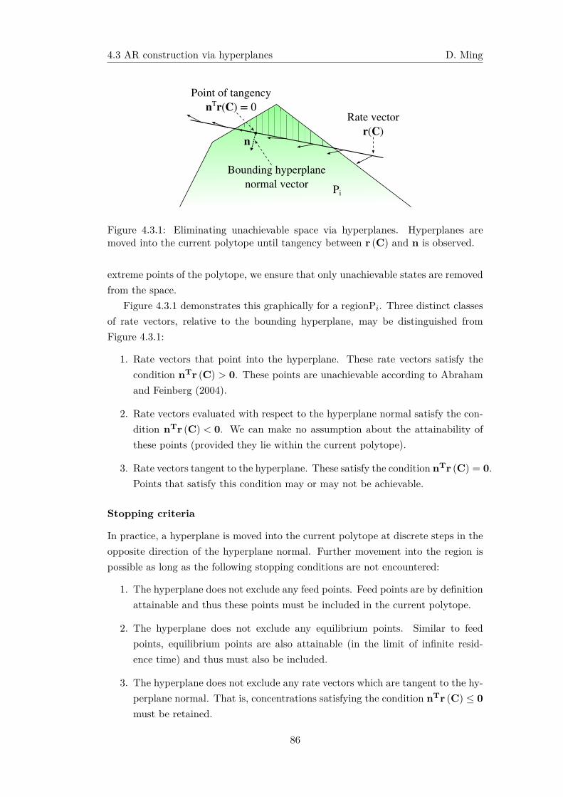
4.3 AR construction via hyperplanes D. Ming
n
Point of tangencynTr(C) = 0
Rate vectorr(C)
Bounding hyperplanenormal vector Pi
Figure 4.3.1: Eliminating unachievable space via hyperplanes. Hyperplanes aremoved into the current polytope until tangency between r (C) and n is observed.
extreme points of the polytope, we ensure that only unachievable states are removedfrom the space.
Figure 4.3.1 demonstrates this graphically for a regionPi. Three distinct classesof rate vectors, relative to the bounding hyperplane, may be distinguished fromFigure 4.3.1:
1. Rate vectors that point into the hyperplane. These rate vectors satisfy thecondition nTr (C) > 0. These points are unachievable according to Abrahamand Feinberg (2004).
2. Rate vectors evaluated with respect to the hyperplane normal satisfy the con-dition nTr (C) < 0. We can make no assumption about the attainability ofthese points (provided they lie within the current polytope).
3. Rate vectors tangent to the hyperplane. These satisfy the condition nTr (C) = 0.Points that satisfy this condition may or may not be achievable.
Stopping criteria
In practice, a hyperplane is moved into the current polytope at discrete steps in theopposite direction of the hyperplane normal. Further movement into the region ispossible as long as the following stopping conditions are not encountered:
1. The hyperplane does not exclude any feed points. Feed points are by definitionattainable and thus these points must be included in the current polytope.
2. The hyperplane does not exclude any equilibrium points. Similar to feedpoints, equilibrium points are also attainable (in the limit of infinite resid-ence time) and thus must also be included.
3. The hyperplane does not exclude any rate vectors which are tangent to the hy-perplane normal. That is, concentrations satisfying the condition nTr (C) ≤ 0must be retained.
86
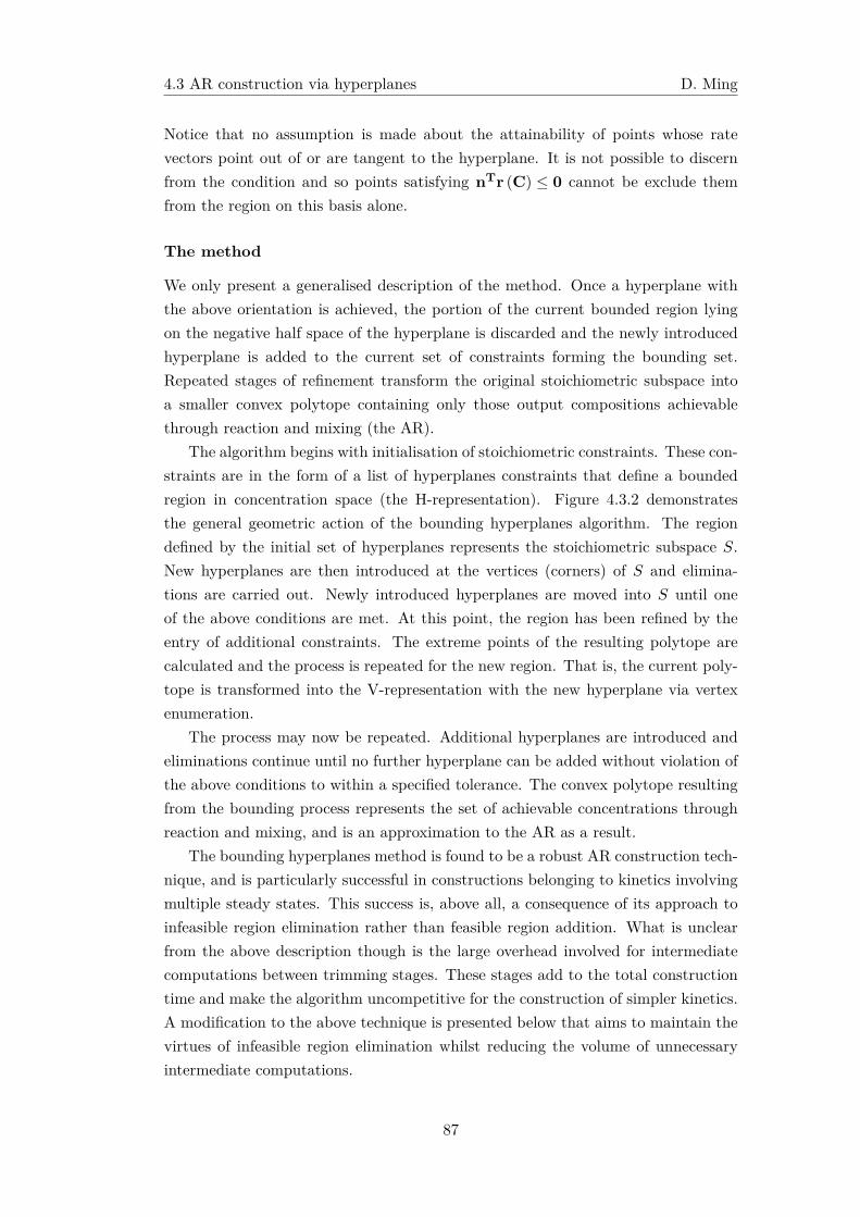
4.3 AR construction via hyperplanes D. Ming
Notice that no assumption is made about the attainability of points whose ratevectors point out of or are tangent to the hyperplane. It is not possible to discernfrom the condition and so points satisfying nTr (C) ≤ 0 cannot be exclude themfrom the region on this basis alone.
The method
We only present a generalised description of the method. Once a hyperplane withthe above orientation is achieved, the portion of the current bounded region lyingon the negative half space of the hyperplane is discarded and the newly introducedhyperplane is added to the current set of constraints forming the bounding set.Repeated stages of refinement transform the original stoichiometric subspace intoa smaller convex polytope containing only those output compositions achievablethrough reaction and mixing (the AR).
The algorithm begins with initialisation of stoichiometric constraints. These con-straints are in the form of a list of hyperplanes constraints that define a boundedregion in concentration space (the H-representation). Figure 4.3.2 demonstratesthe general geometric action of the bounding hyperplanes algorithm. The regiondefined by the initial set of hyperplanes represents the stoichiometric subspace S.New hyperplanes are then introduced at the vertices (corners) of S and elimina-tions are carried out. Newly introduced hyperplanes are moved into S until oneof the above conditions are met. At this point, the region has been refined by theentry of additional constraints. The extreme points of the resulting polytope arecalculated and the process is repeated for the new region. That is, the current poly-tope is transformed into the V-representation with the new hyperplane via vertexenumeration.
The process may now be repeated. Additional hyperplanes are introduced andeliminations continue until no further hyperplane can be added without violation ofthe above conditions to within a specified tolerance. The convex polytope resultingfrom the bounding process represents the set of achievable concentrations throughreaction and mixing, and is an approximation to the AR as a result.
The bounding hyperplanes method is found to be a robust AR construction tech-nique, and is particularly successful in constructions belonging to kinetics involvingmultiple steady states. This success is, above all, a consequence of its approach toinfeasible region elimination rather than feasible region addition. What is unclearfrom the above description though is the large overhead involved for intermediatecomputations between trimming stages. These stages add to the total constructiontime and make the algorithm uncompetitive for the construction of simpler kinetics.A modification to the above technique is presented below that aims to maintain thevirtues of infeasible region elimination whilst reducing the volume of unnecessaryintermediate computations.
87
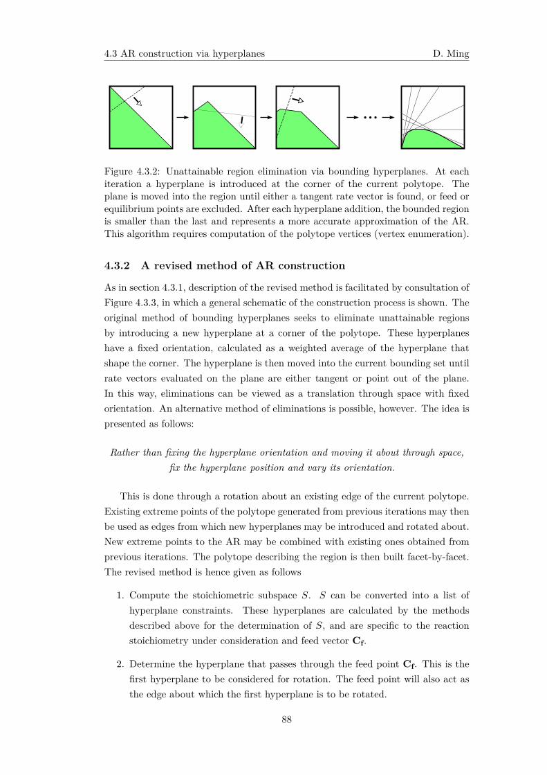
4.3 AR construction via hyperplanes D. Ming
...
Figure 4.3.2: Unattainable region elimination via bounding hyperplanes. At eachiteration a hyperplane is introduced at the corner of the current polytope. Theplane is moved into the region until either a tangent rate vector is found, or feed orequilibrium points are excluded. After each hyperplane addition, the bounded regionis smaller than the last and represents a more accurate approximation of the AR.This algorithm requires computation of the polytope vertices (vertex enumeration).
4.3.2 A revised method of AR construction
As in section 4.3.1, description of the revised method is facilitated by consultation ofFigure 4.3.3, in which a general schematic of the construction process is shown. Theoriginal method of bounding hyperplanes seeks to eliminate unattainable regionsby introducing a new hyperplane at a corner of the polytope. These hyperplaneshave a fixed orientation, calculated as a weighted average of the hyperplane thatshape the corner. The hyperplane is then moved into the current bounding set untilrate vectors evaluated on the plane are either tangent or point out of the plane.In this way, eliminations can be viewed as a translation through space with fixedorientation. An alternative method of eliminations is possible, however. The idea ispresented as follows:
Rather than fixing the hyperplane orientation and moving it about through space,fix the hyperplane position and vary its orientation.
This is done through a rotation about an existing edge of the current polytope.Existing extreme points of the polytope generated from previous iterations may thenbe used as edges from which new hyperplanes may be introduced and rotated about.New extreme points to the AR may be combined with existing ones obtained fromprevious iterations. The polytope describing the region is then built facet-by-facet.The revised method is hence given as follows
1. Compute the stoichiometric subspace S. S can be converted into a list ofhyperplane constraints. These hyperplanes are calculated by the methodsdescribed above for the determination of S, and are specific to the reactionstoichiometry under consideration and feed vector Cf.
2. Determine the hyperplane that passes through the feed point Cf. This is thefirst hyperplane to be considered for rotation. The feed point will also act asthe edge about which the first hyperplane is to be rotated.
88
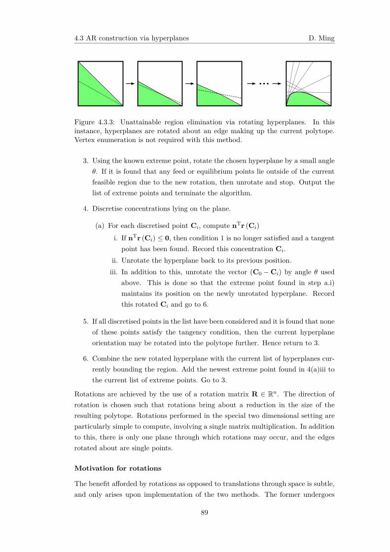
4.3 AR construction via hyperplanes D. Ming
...
Figure 4.3.3: Unattainable region elimination via rotating hyperplanes. In thisinstance, hyperplanes are rotated about an edge making up the current polytope.Vertex enumeration is not required with this method.
3. Using the known extreme point, rotate the chosen hyperplane by a small angleθ. If it is found that any feed or equilibrium points lie outside of the currentfeasible region due to the new rotation, then unrotate and stop. Output thelist of extreme points and terminate the algorithm.
4. Discretise concentrations lying on the plane.
(a) For each discretised point Ci, compute nTr (Ci)
i. If nTr (Ci) ≤ 0, then condition 1 is no longer satisfied and a tangentpoint has been found. Record this concentration Ci.
ii. Unrotate the hyperplane back to its previous position.iii. In addition to this, unrotate the vector (C0 − Ci) by angle θ used
above. This is done so that the extreme point found in step a.i)maintains its position on the newly unrotated hyperplane. Recordthis rotated Ci and go to 6.
5. If all discretised points in the list have been considered and it is found that noneof these points satisfy the tangency condition, then the current hyperplaneorientation may be rotated into the polytope further. Hence return to 3.
6. Combine the new rotated hyperplane with the current list of hyperplanes cur-rently bounding the region. Add the newest extreme point found in 4(a)iii tothe current list of extreme points. Go to 3.
Rotations are achieved by the use of a rotation matrix R ∈ Rn. The direction ofrotation is chosen such that rotations bring about a reduction in the size of theresulting polytope. Rotations performed in the special two dimensional setting areparticularly simple to compute, involving a single matrix multiplication. In additionto this, there is only one plane through which rotations may occur, and the edgesrotated about are single points.
Motivation for rotations
The benefit afforded by rotations as opposed to translations through space is subtle,and only arises upon implementation of the two methods. The former undergoes
89
4.3 AR construction via hyperplanes D. Ming
two computationally intensive, yet entirely necessary, stages.
1. The first, which is common to both approaches, is the act of hyperplane discret-isation (computing distinct points lying on the hyperplane and then checkingthe rate vector at each point). Since a hyperplane represents an n − 1 di-mensional subspace in Rn, hyperplane discretisation may be viewed as a com-putational process of degree n − 1. Adopting Big-O notation, the number offloating point operations (flops) for such a process is proportional to approx-imately O(Mn−1), where M is the number of discretised points for each axisin space and n is the dimension of the computational space (the dimension ofS).
2. The second intensive computation is altogether suppressed during the earlystages of refinement but quickly emerges as the number of bounding hyper-planes increases throughout construction. In order for new hyperplanes to beintroduced, we must know the locations of the extreme points of the polytope,defined by the current list of hyperplanes. That is, for each iteration of theelimination process, the vertex enumeration problem must be solved. This is anon-trivial problem, particularly for higher dimensional spaces involving manyhyperplanes. A brute-force implementation can be achieved by computing theintersection of each plane with every other hyperplane in the region: Given L
hyperplanes in Rn, brute-force computation results in at most L!/ [n! (L− n)!]
total intersections that must be calculated, and hence this method is not re-commended. More efficient methods exist that solve the problem in polynomialtime (Dyer, 1983), potentially alleviating part of the computational burden,although a vertex enumeration step is nevertheless required in order for elim-inations to be carried out.A final consideration is the issue of redundant hyperplanes, that is, hyperplanesthat play no useful role in defining the feasible region. It is wise to excludethese from the set of bounding constraints as quickly as possible though, asthe numbers of redundant hyperplanes can quickly outnumber the number ofuseful planes describing the feasible region. This ultimately affects the vertexenumeration step in an undesirable manner. As a result, the additional expenseof redundant hyperplane removal contributes further to the total computationtime of the bounding process.
The benefit of utilising hyperplane rotations as opposed to translations is that theformer does not require the enumeration of vertices (point 2). As a result, the costlyexercise of redundant hyperplane removal and vertex enumeration stages may beavoided. This is accomplished by the addition policy of the revised method. Sincerotations are done about existing, known attainable points, the hyperplane tangencycondition guarantees that the new extreme point found is (in R2) attainable byCSTR from eq 2.3.2. Hence, at every stage of construction, boundary points of the
90
4.4 Examples D. Ming
AR are found, and intermediate points never enter the problem. The enumeration ofvertices is still an unnecessary computation however. We refer the reader to section4.6 for a discussion on how constructions might be carried out in higher dimensions.
Although it is the aim to achieve candidate AR constructions via an eliminationof unachievable space, this can be carried in a number of ways. The use of hyperplanerotations is one such method which is, in principle, no different to the method ofbounding hyperplanes – both methods ultimately rely on the tangency conditionwith the rate vector, as discussed above. However, the use of rotations is observedto be faster in practice. We demonstrate this with a number of examples below.
4.4 Examples
4.4.1 Isothermal constructions
van de Vusse kinetics
We now demonstrate how the method of bounding hyperplanes may be improved byplane rotations for various examples. In all the examples presented, we have assumedthat the systems are operated isothermally and under constant density. Althoughwe shall later present an example in which the isothermal assumption is relaxed, wehonour this restriction for purposes of comparison to the original method.
We begin with the well understood van de Vusse reaction scheme. The systemis given by the following set of reactions:
Ak1k2
B k3→ C
2A →k4
D(4.4.1)
Several variations of the above kinetics exist but only the simplest scenario is presen-ted here, that is a 2D system in cA − cB space with mass action kinetics given bythe following constants k1 = 1.0, k2 = 0.0, k3 = 1.0 and k4 = 20.0, such that
r (C) =
[−k1cA + k2cB − 2k4c
2A
k1cA − k2cB − k3cB
]
The AR is then found to be produced by a CSTR followed in series by a PFR.Unfortunately this arrangement cannot be established by the algorithm, but hasbeen included to demonstrate the accuracy to which constructions may agree withtheir theoretical predictions. A worked example for the first iteration of this problemcan be found in appendix B.1. Here, the reader will find details discussing thenecessary set-up steps required before the algorithm can be initialised. The resultsof the construction are given by Figure 4.4.1 below where a comparison is madebetween the original (translated) and revised (rotated) methods.
91
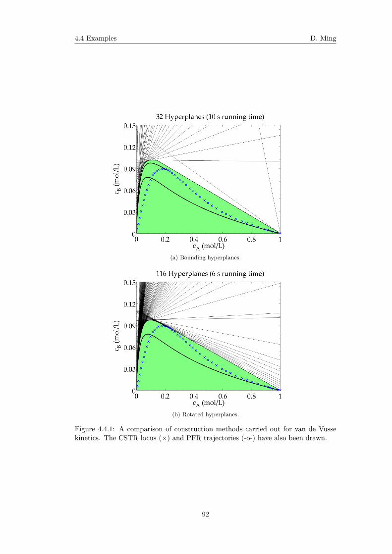
4.4 Examples D. Ming
(a) Bounding hyperplanes.
(b) Rotated hyperplanes.
Figure 4.4.1: A comparison of construction methods carried out for van de Vussekinetics. The CSTR locus (×) and PFR trajectories (-o-) have also been drawn.
92
4.4 Examples D. Ming
The total running time for the original method took 10 seconds and is boundedby 32 hyperplanes. The shape of the boundary produced by the original methodagrees with the analytical solution although a distinct difference between the two isnoticeable near the CSTR-PFR junction. In particular, the maximum concentrationof component B is overestimated slightly with the original method. The resultsachieved with the revised approach by comparison are in close agreement with thetheory. The time taken to construct the new region took 6 seconds and is constructedwith 116 hyperplanes. Although running time is of a similar order to the former,the region is assembled with a significantly larger number of hyperplanes, allowingfor a more precise bound to be established.
The results highlight an important consideration associated with both methods.That is, there is no claim that the resulting polytope obtained from construction isindeed the true AR. Rather, the results provide an upper bound on kinetic attainab-ility. Certainly there is evidence to suggest that in the limit as more hyperplanes areused to bound the region, we approach the true AR boundary, however the regionsobtained by either method are necessarily always larger than the true solution. Ifboth an inside-out and outside-in method are available, then comparison betweenthe two candidate ARs may allow for the determination of the true AR boundary. Ifthe results of the two do not correspond, then a closer bound on the true boundaryis reached as we know that the true region must lie between the two constructions.
Complex van de Vusse kinetics
Next we study a fairly artificial example, one in which highly non-linear behaviouris observed. This may be produced by the following rates of formation
rA (C) = f (cA)2 + cAcB
df (cA)
dcArB (C) = cAf (cA)
wheref (cA) = 6c6A − 6c5A + 9c4A − 16c3A + 9c2A − 2cA
The reaction scheme is identical to the one posed for regular van de Vusse kineticsby eq 4.4.1, although the actual rate expressions are more complicated now. APFR trajectory associated with the kinetics given above show multiple concavities,indicating that both reaction and mixing processes will feature prominently in theformation of the AR boundary. Indeed, it is found that for a feed concentration ofCf = [1, 0]T, the AR is constructed from a four reactor series network of CSTR-PFR-CSTR-PFR (Glasser et al., 1987). Figure 4.4.2 provides results obtained fromboth methods of construction.
Once again, both the original and revised methods allow for an accurate approx-imation of the AR boundary, even for highly non-linear kinetics. The efficiency by
93
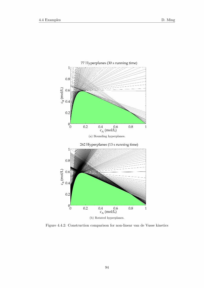
4.4 Examples D. Ming
(a) Bounding hyperplanes.
(b) Rotated hyperplanes.
Figure 4.4.2: Construction comparison for non-linear van de Vusse kinetics
94
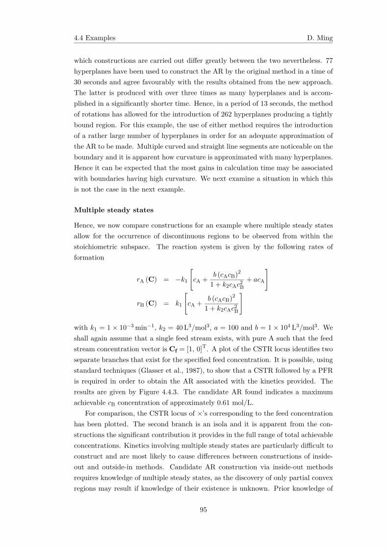
4.4 Examples D. Ming
which constructions are carried out differ greatly between the two nevertheless. 77hyperplanes have been used to construct the AR by the original method in a time of30 seconds and agree favourably with the results obtained from the new approach.The latter is produced with over three times as many hyperplanes and is accom-plished in a significantly shorter time. Hence, in a period of 13 seconds, the methodof rotations has allowed for the introduction of 262 hyperplanes producing a tightlybound region. For this example, the use of either method requires the introductionof a rather large number of hyperplanes in order for an adequate approximation ofthe AR to be made. Multiple curved and straight line segments are noticeable on theboundary and it is apparent how curvature is approximated with many hyperplanes.Hence it can be expected that the most gains in calculation time may be associatedwith boundaries having high curvature. We next examine a situation in which thisis not the case in the next example.
Multiple steady states
Hence, we now compare constructions for an example where multiple steady statesallow for the occurrence of discontinuous regions to be observed from within thestoichiometric subspace. The reaction system is given by the following rates offormation
rA (C) = −k1
[cA +
b (cAcB)2
1 + k2cAc2B+ acA
]
rB (C) = k1
[cA +
b (cAcB)2
1 + k2cAc2B
]
with k1 = 1 × 10⁻³ min−1, k2 = 40L3/mol3, a = 100 and b = 1 × 10⁴ L3/mol3. Weshall again assume that a single feed stream exists, with pure A such that the feedstream concentration vector is Cf = [1, 0]T. A plot of the CSTR locus identifies twoseparate branches that exist for the specified feed concentration. It is possible, usingstandard techniques (Glasser et al., 1987), to show that a CSTR followed by a PFRis required in order to obtain the AR associated with the kinetics provided. Theresults are given by Figure 4.4.3. The candidate AR found indicates a maximumachievable cB concentration of approximately 0.61 mol/L.
For comparison, the CSTR locus of ×’s corresponding to the feed concentrationhas been plotted. The second branch is an isola and it is apparent from the con-structions the significant contribution it provides in the full range of total achievableconcentrations. Kinetics involving multiple steady states are particularly difficult toconstruct and are most likely to cause differences between constructions of inside-out and outside-in methods. Candidate AR construction via inside-out methodsrequires knowledge of multiple steady states, as the discovery of only partial convexregions may result if knowledge of their existence is unknown. Prior knowledge of
95
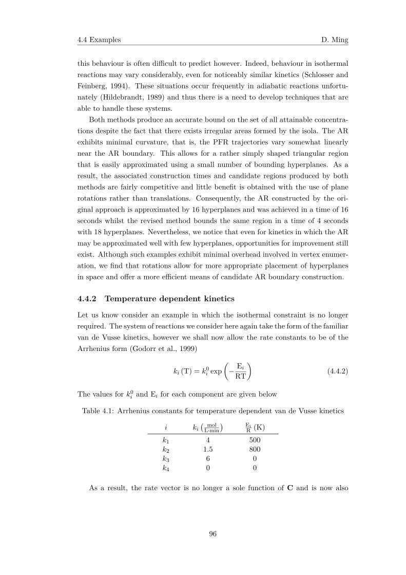
4.4 Examples D. Ming
this behaviour is often difficult to predict however. Indeed, behaviour in isothermalreactions may vary considerably, even for noticeably similar kinetics (Schlosser andFeinberg, 1994). These situations occur frequently in adiabatic reactions unfortu-nately (Hildebrandt, 1989) and thus there is a need to develop techniques that areable to handle these systems.
Both methods produce an accurate bound on the set of all attainable concentra-tions despite the fact that there exists irregular areas formed by the isola. The ARexhibits minimal curvature, that is, the PFR trajectories vary somewhat linearlynear the AR boundary. This allows for a rather simply shaped triangular regionthat is easily approximated using a small number of bounding hyperplanes. As aresult, the associated construction times and candidate regions produced by bothmethods are fairly competitive and little benefit is obtained with the use of planerotations rather than translations. Consequently, the AR constructed by the ori-ginal approach is approximated by 16 hyperplanes and was achieved in a time of 16seconds whilst the revised method bounds the same region in a time of 4 secondswith 18 hyperplanes. Nevertheless, we notice that even for kinetics in which the ARmay be approximated well with few hyperplanes, opportunities for improvement stillexist. Although such examples exhibit minimal overhead involved in vertex enumer-ation, we find that rotations allow for more appropriate placement of hyperplanesin space and offer a more efficient means of candidate AR boundary construction.
4.4.2 Temperature dependent kinetics
Let us know consider an example in which the isothermal constraint is no longerrequired. The system of reactions we consider here again take the form of the familiarvan de Vusse kinetics, however we shall now allow the rate constants to be of theArrhenius form (Godorr et al., 1999)
ki (T) = k0i exp(− Ei
RT
)(4.4.2)
The values for k0i and Ei for each component are given below
Table 4.1: Arrhenius constants for temperature dependent van de Vusse kinetics
i ki( mol
L·min) Ei
R (K)
k1 4 500k2 1.5 800k3 6 0k4 0 0
As a result, the rate vector is no longer a sole function of C and is now also
96
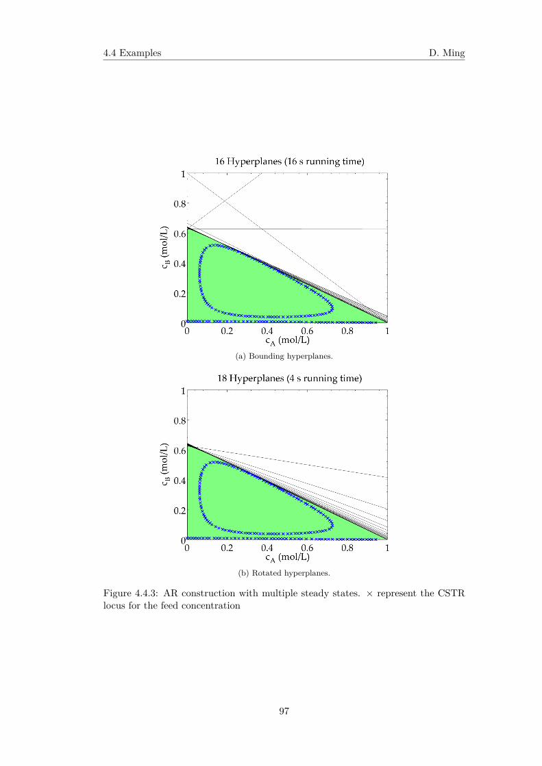
4.4 Examples D. Ming
(a) Bounding hyperplanes.
(b) Rotated hyperplanes.
Figure 4.4.3: AR construction with multiple steady states. × represent the CSTRlocus for the feed concentration
97
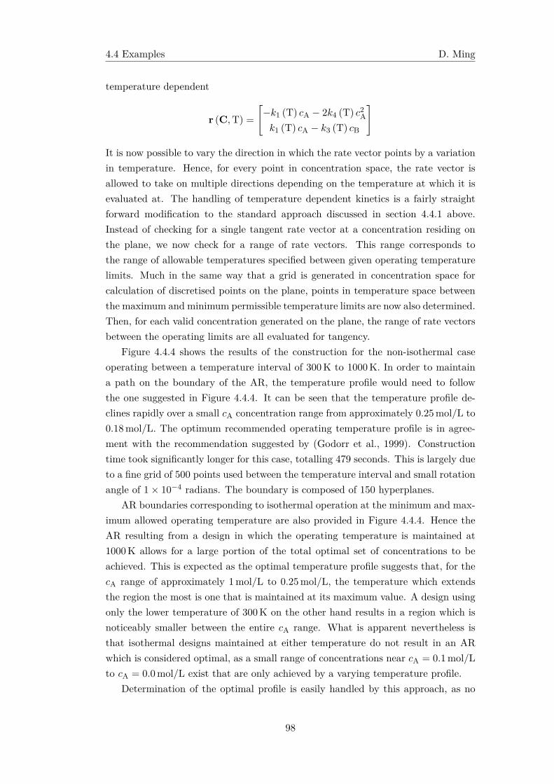
4.4 Examples D. Ming
temperature dependent
r (C,T) =
[−k1 (T) cA − 2k4 (T) c2Ak1 (T) cA − k3 (T) cB
]
It is now possible to vary the direction in which the rate vector points by a variationin temperature. Hence, for every point in concentration space, the rate vector isallowed to take on multiple directions depending on the temperature at which it isevaluated at. The handling of temperature dependent kinetics is a fairly straightforward modification to the standard approach discussed in section 4.4.1 above.Instead of checking for a single tangent rate vector at a concentration residing onthe plane, we now check for a range of rate vectors. This range corresponds tothe range of allowable temperatures specified between given operating temperaturelimits. Much in the same way that a grid is generated in concentration space forcalculation of discretised points on the plane, points in temperature space betweenthe maximum and minimum permissible temperature limits are now also determined.Then, for each valid concentration generated on the plane, the range of rate vectorsbetween the operating limits are all evaluated for tangency.
Figure 4.4.4 shows the results of the construction for the non-isothermal caseoperating between a temperature interval of 300 K to 1000 K. In order to maintaina path on the boundary of the AR, the temperature profile would need to followthe one suggested in Figure 4.4.4. It can be seen that the temperature profile de-clines rapidly over a small cA concentration range from approximately 0.25 mol/L to0.18 mol/L. The optimum recommended operating temperature profile is in agree-ment with the recommendation suggested by (Godorr et al., 1999). Constructiontime took significantly longer for this case, totalling 479 seconds. This is largely dueto a fine grid of 500 points used between the temperature interval and small rotationangle of 1× 10⁻⁴ radians. The boundary is composed of 150 hyperplanes.
AR boundaries corresponding to isothermal operation at the minimum and max-imum allowed operating temperature are also provided in Figure 4.4.4. Hence theAR resulting from a design in which the operating temperature is maintained at1000 K allows for a large portion of the total optimal set of concentrations to beachieved. This is expected as the optimal temperature profile suggests that, for thecA range of approximately 1 mol/L to 0.25 mol/L, the temperature which extendsthe region the most is one that is maintained at its maximum value. A design usingonly the lower temperature of 300 K on the other hand results in a region which isnoticeably smaller between the entire cA range. What is apparent nevertheless isthat isothermal designs maintained at either temperature do not result in an ARwhich is considered optimal, as a small range of concentrations near cA = 0.1mol/Lto cA = 0.0mol/L exist that are only achieved by a varying temperature profile.
Determination of the optimal profile is easily handled by this approach, as no
98
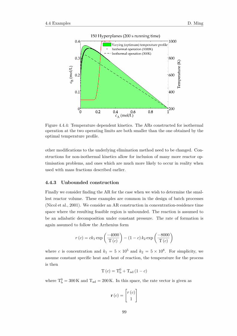
4.4 Examples D. Ming
Figure 4.4.4: Temperature dependent kinetics. The ARs constructed for isothermaloperation at the two operating limits are both smaller than the one obtained by theoptimal temperature profile.
other modifications to the underlying elimination method need to be changed. Con-structions for non-isothermal kinetics allow for inclusion of many more reactor op-timisation problems, and ones which are much more likely to occur in reality whenused with mass fractions described earlier.
4.4.3 Unbounded construction
Finally we consider finding the AR for the case when we wish to determine the smal-lest reactor volume. These examples are common in the design of batch processes(Nicol et al., 2001). We consider an AR construction in concentration-residence timespace where the resulting feasible region is unbounded. The reaction is assumed tobe an adiabatic decomposition under constant pressure. The rate of formation isagain assumed to follow the Arrhenius form
r (c) = ck1 exp(−4000T (c)
)− (1− c) k2 exp
(−8000T (c)
)where c is concentration and k1 = 5 × 10⁵ and k2 = 5 × 10⁸. For simplicity, weassume constant specific heat and heat of reaction, the temperature for the processis then
T (c) = T0b + Tad (1− c)
where T0b = 300K and Tad = 200K. In this space, the rate vector is given as
r (c) =[r (c)
1
]
99
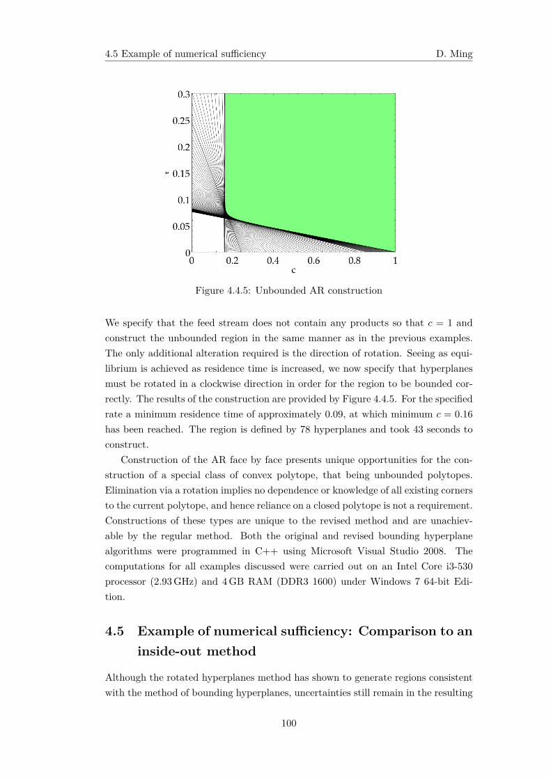
4.5 Example of numerical sufficiency D. Ming
Figure 4.4.5: Unbounded AR construction
We specify that the feed stream does not contain any products so that c = 1 andconstruct the unbounded region in the same manner as in the previous examples.The only additional alteration required is the direction of rotation. Seeing as equi-librium is achieved as residence time is increased, we now specify that hyperplanesmust be rotated in a clockwise direction in order for the region to be bounded cor-rectly. The results of the construction are provided by Figure 4.4.5. For the specifiedrate a minimum residence time of approximately 0.09, at which minimum c = 0.16
has been reached. The region is defined by 78 hyperplanes and took 43 seconds toconstruct.
Construction of the AR face by face presents unique opportunities for the con-struction of a special class of convex polytope, that being unbounded polytopes.Elimination via a rotation implies no dependence or knowledge of all existing cornersto the current polytope, and hence reliance on a closed polytope is not a requirement.Constructions of these types are unique to the revised method and are unachiev-able by the regular method. Both the original and revised bounding hyperplanealgorithms were programmed in C++ using Microsoft Visual Studio 2008. Thecomputations for all examples discussed were carried out on an Intel Core i3-530processor (2.93GHz) and 4GB RAM (DDR3 1600) under Windows 7 64-bit Edi-tion.
4.5 Example of numerical sufficiency: Comparison to aninside-out method
Although the rotated hyperplanes method has shown to generate regions consistentwith the method of bounding hyperplanes, uncertainties still remain in the resulting
100
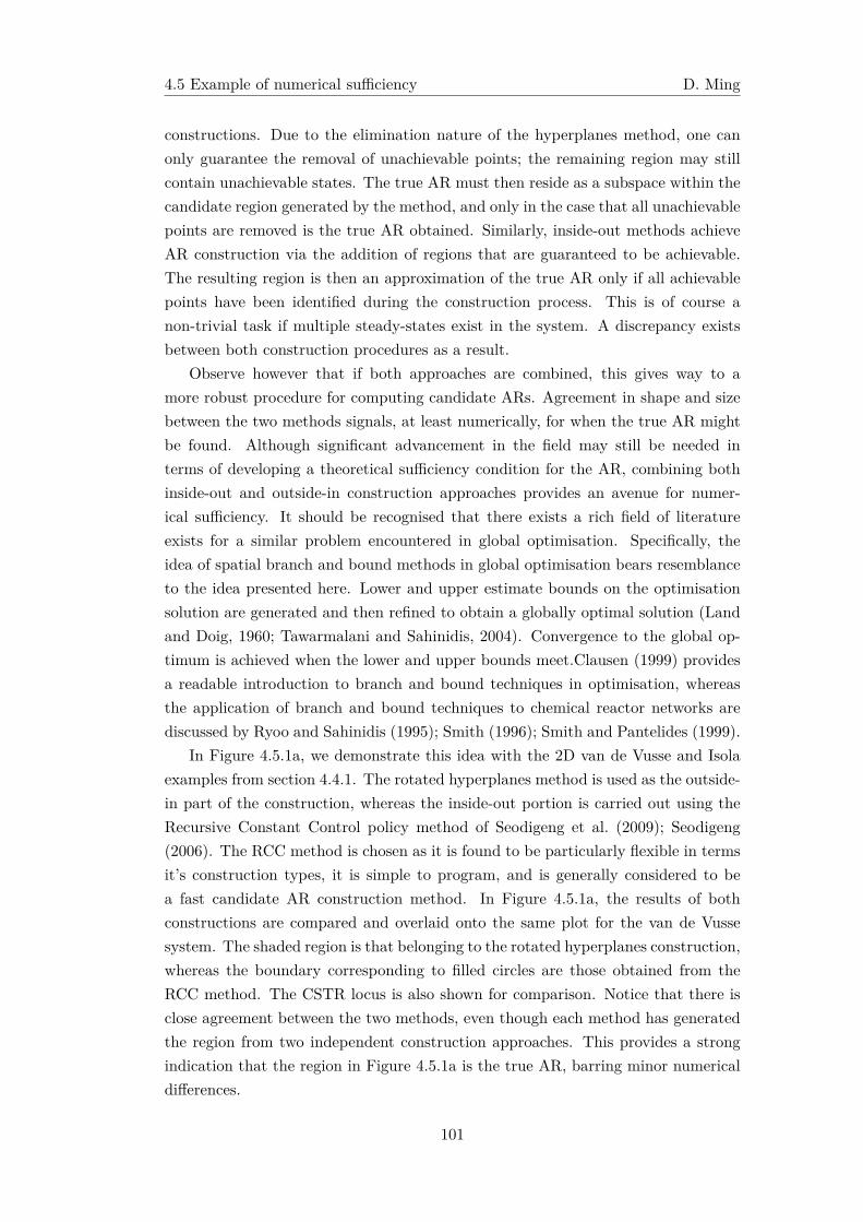
4.5 Example of numerical sufficiency D. Ming
constructions. Due to the elimination nature of the hyperplanes method, one canonly guarantee the removal of unachievable points; the remaining region may stillcontain unachievable states. The true AR must then reside as a subspace within thecandidate region generated by the method, and only in the case that all unachievablepoints are removed is the true AR obtained. Similarly, inside-out methods achieveAR construction via the addition of regions that are guaranteed to be achievable.The resulting region is then an approximation of the true AR only if all achievablepoints have been identified during the construction process. This is of course anon-trivial task if multiple steady-states exist in the system. A discrepancy existsbetween both construction procedures as a result.
Observe however that if both approaches are combined, this gives way to amore robust procedure for computing candidate ARs. Agreement in shape and sizebetween the two methods signals, at least numerically, for when the true AR mightbe found. Although significant advancement in the field may still be needed interms of developing a theoretical sufficiency condition for the AR, combining bothinside-out and outside-in construction approaches provides an avenue for numer-ical sufficiency. It should be recognised that there exists a rich field of literatureexists for a similar problem encountered in global optimisation. Specifically, theidea of spatial branch and bound methods in global optimisation bears resemblanceto the idea presented here. Lower and upper estimate bounds on the optimisationsolution are generated and then refined to obtain a globally optimal solution (Landand Doig, 1960; Tawarmalani and Sahinidis, 2004). Convergence to the global op-timum is achieved when the lower and upper bounds meet.Clausen (1999) providesa readable introduction to branch and bound techniques in optimisation, whereasthe application of branch and bound techniques to chemical reactor networks arediscussed by Ryoo and Sahinidis (1995); Smith (1996); Smith and Pantelides (1999).
In Figure 4.5.1a, we demonstrate this idea with the 2D van de Vusse and Isolaexamples from section 4.4.1. The rotated hyperplanes method is used as the outside-in part of the construction, whereas the inside-out portion is carried out using theRecursive Constant Control policy method of Seodigeng et al. (2009); Seodigeng(2006). The RCC method is chosen as it is found to be particularly flexible in termsit’s construction types, it is simple to program, and is generally considered to bea fast candidate AR construction method. In Figure 4.5.1a, the results of bothconstructions are compared and overlaid onto the same plot for the van de Vussesystem. The shaded region is that belonging to the rotated hyperplanes construction,whereas the boundary corresponding to filled circles are those obtained from theRCC method. The CSTR locus is also shown for comparison. Notice that there isclose agreement between the two methods, even though each method has generatedthe region from two independent construction approaches. This provides a strongindication that the region in Figure 4.5.1a is the true AR, barring minor numericaldifferences.
101
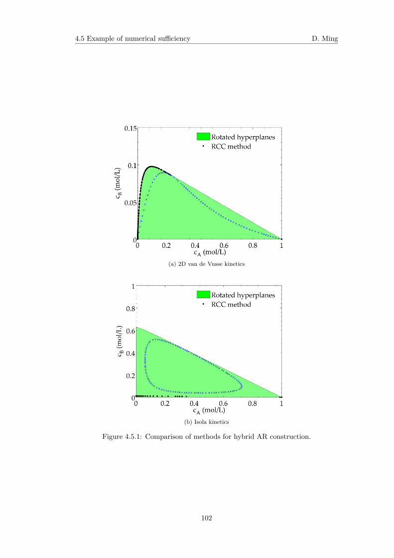
4.5 Example of numerical sufficiency D. Ming
(a) 2D van de Vusse kinetics
(b) Isola kinetics
Figure 4.5.1: Comparison of methods for hybrid AR construction.
102
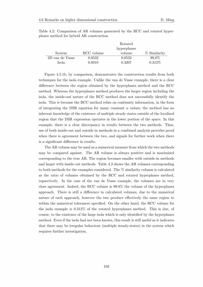
4.6 Remarks on higher dimensional construction D. Ming
Table 4.2: Comparison of AR volumes generated by the RCC and rotated hyper-planes method for hybrid AR construction
System RCC volume
Rotatedhyperplanes
volume % Similarity2D van de Vusse 0.0532 0.0533 99.8%
Isola 0.0010 0.3207 0.312%
Figure 4.5.1b, by comparison, demonstrates the construction results from bothtechniques for the isola example. Unlike the van de Vusse example, there is a cleardifference between the region obtained by the hyperplanes method and the RCCmethod. Whereas the hyperplanes method produces the larger region including theisola, the inside-out nature of the RCC method does not successfully identify theisola. This is because the RCC method relies on continuity information, in the formof integrating the DSR equation for many constant α values; the method has noinherent knowledge of the existence of multiple steady states outside of the localisedregion that the DSR expression operates in the lower portion of the space. In thisexample, there is a clear discrepancy in results between the two methods. Thus,use of both inside-out and outside in methods in a combined analysis provides proofwhen there is agreement between the two, and signals for further work when thereis a significant difference in results.
The AR volume may be used as a numerical measure from which the two methodsmay be compared against. The AR volume is always positive and is maximisedcorresponding to the true AR. The region becomes smaller with outside-in methodsand larger with inside-out methods. Table 4.2 shows the AR volumes correspondingto both methods for the examples considered. The % similarity column is calculatedas the ratio of volumes obtained by the RCC and rotated hyperplanes method,repsectively. In the case of the van de Vusse example, the volumes are in veryclose agreement. Indeed, the RCC volume is 99.8% the volume of the hyperplanesapproach. There is still a difference in calculated volumes, due to the numericalnature of each approach, however the two produce effectively the same region towithin the numerical tolerances specified. On the other hand, the RCC volume forthe isola example is 0.312% of the rotated hyperplanes method. This is due, ofcourse, to the existence of the large isola which is only identified by the hyperplanesmethod. Even if the isola had not been known, this result is still useful as it indicatesthat there may be irregular behaviour (multiple steady-states) in the system whichrequires further investigation.
103
4.6 Remarks on higher dimensional construction D. Ming
4.6 Remarks on higher dimensional construction
4.6.1 Introduction
Constructions in Rn are currently not yet fully developed, however several ideasare provided below for how they might be carried out. The expected complicationsinvolved in generalised n-dimensional constructions are also discussed. In order toextend the method of rotation to higher dimensions, we must first have an under-standing of how these may be generalised, in spaces that cannot be easily visualised.First, a generalised description of rotations is discussed which describes how thisis achieved in Rn. Next, supporting mathematical details are given, followed bya proposed method for extension to higher dimensions. A brief discussion on thepotential difficulties and uncertainties with the approach is then supplied at the end.
4.6.2 Rotations in Rn
Facets and ridges
Before a generalised discussion can be done, a basic understanding of the facetsand ridges, associated with an n-dimensional convex polytope, must be known. Wesymbolise the convex polytope associated with the a candidate AR construction byconv(X). From section 4.2.4, a facet of conv(X) is a collection of extreme points suchthat n linearly independent points in conv(X) lie on a hyperplane H (n,C0) residingin Rn. A facet is hence a (n− 1)-dimensional polytope in Rn and a subspace ofconv(X) – two vertices define a facet in R2, three in R3, and so on.
Ridges (edges) of conv(X) are similar in structure to facets. Indeed, a ridgeis composed of vertices from a facet and hence it is a linear subspace of a facet.Specifically, n − 1 linearly independent points of a facet create a ridge. A ridge ishence a (n− 2)-dimensional polytope, and for any facet containing n vertices, thereare n − 1 ridges that are associated with it. The intersection of two facets createsa ridge. This is show in Figure 4.6.1a for two and three dimensions. A distinctionis made between ridges and edges since edges are generally viewed with specificreference to three dimensions, whereas ridges are generalised for all dimensions.
General understanding
Rotations in higher dimensions are more challenging than those cast in R2 alone.This originates primarily from the fact there are more ways in which to rotate aplane in higher dimensional space. By example, in R3 there are three principle axisthat a hyperplane can be rotated about (the standard basis involving x, y and zaxes are an example of this). In general, there are
(n2
)principle axes in Rn and thus
rotations in higher dimensions are not uniquely defined (Aguilera and Perez-Aguila,2004). Moreover, the view of rotations in R2 and R3 can be misleading. That is,
104
4.6 Remarks on higher dimensional construction D. Ming
rotations are often viewed to occur about an axis of rotation (a one-dimensionalsubspace of Rn). From the previous statements, simply fixing the dimension forrotation only reduces the number of degrees of freedom for rotation by one, but forspaces greater than three, there are more principle axes from which rotations maystill occur. Hence the understanding of rotations to occur about an axis of rotation(an edge) is only convenient for systems in R3.
Instead, it is better to view rotations in terms of a rotation in a plane. Pointsin space are then transformed with respect to the plane of rotation and a spaceorthogonal to the plane. The component of the point in the orthogonal subspaceis hence unchanged by the action of a rotation. Rotations are therefore still twodimensional in nature, even when considered in higher dimensions. In Figure 4.6.1bwe show this for R3, although the method is true for all dimensions.
We can generalise the idea of an edge and instead view rotations to occur abouta ridge. Since a ridge is a n − 2 dimensional subspace of Rn, this leaves a twodimensional subspace about which points may be rotated in. Rotation are then notarbitrary, but rather are aligned with ridges from existing facets.
4.6.3 Additional mathematical details
Change of basis
A vector x viewed under one coordinate system can be written with respect toanother by a change of basis. That is, given an general matrix A containing k
linearly independent vectors forming a basis
A = [a1, a2, . . . , ak]
where k ≤ n, the matrix multiplication
Ay = x
implies that x can be written as a linear combination of the columns of matrix A.Elements in y are then scalar ‘weights’ that give the relative proportions of thecolumns of A used to express x. Vector y is hence a k-dimensional vector thatre-expresses x with respect to the new basis defined by A. Observe that A need notbe square (the columns of A form a subspace of Rn) and the columns of A need notbe orthogonal (although it is useful is the columns of A form an orthonormal basis).
Rotation matrix
The rotation matrix
R =
[cos (θ) −sin (θ)
sin (θ) cos (θ)
](4.6.1)
105
4.6 Remarks on higher dimensional construction D. Ming
rotates a vector Ci ∈ R2 by an angle θ in the plane when R is multiplied to Ci. Itfollows that a rotated vector C′
i ∈ R2 is given by
C′i = RCi
By definition, rotations preserve lengths and angles. We can see that the action of Rmight also be viewed as a change of basis in which lengths and angles are preserved.
Projections onto a plane and the orthogonal complement
Suppose that A is a matrix containing k linearly independent vectors in Rn (A isa matrix of size n × k). An arbitrary vector Ci ∈ Rn can be projected onto thesubspace spanned by the columns of A with the following matrix
P = A(ATA
)−1 AT
We call matrix P the projection matrix and the matrix product PCi the projection ofCi onto the subspace spanned by A. If A contains two linearly independent vectors(k = 2), the subspace spanned by A is a two-dimensional plane in Rn. In general,we can express vector Ci as the sum of two vectors:
Ci = PCi + e
where PCi is the projection of Ci onto a subspace, and e is a vector orthogonal tothe subspace. Vectore is said to be the orthogonal complement of Ci. Given A andCi, the orthogonal complement can be found by rearranging the above expressionfor e
e = Ci − PCi
= (I − P)Ci (4.6.2)
where I is the identity matrix. Observe that if the columns of A form an orthonormalbasis, then the projection matrix P may be simplified:
P = AAT
sinceATA = I (4.6.3)
if A is an orthogonal matrix.
106
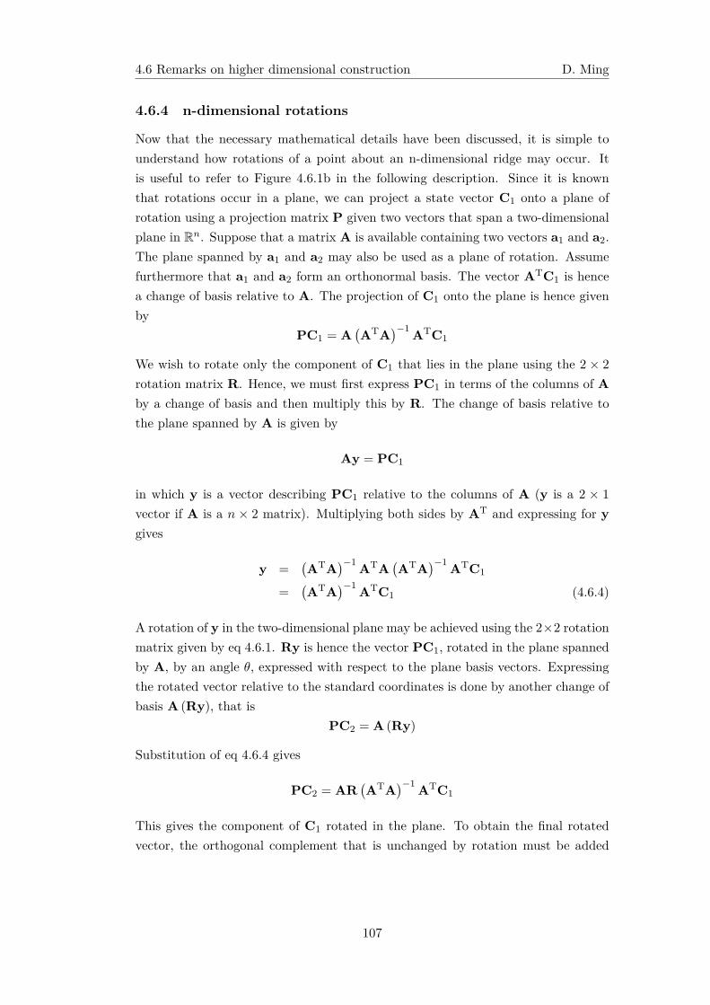
4.6 Remarks on higher dimensional construction D. Ming
4.6.4 n-dimensional rotations
Now that the necessary mathematical details have been discussed, it is simple tounderstand how rotations of a point about an n-dimensional ridge may occur. Itis useful to refer to Figure 4.6.1b in the following description. Since it is knownthat rotations occur in a plane, we can project a state vector C1 onto a plane ofrotation using a projection matrix P given two vectors that span a two-dimensionalplane in Rn. Suppose that a matrix A is available containing two vectors a1 and a2.The plane spanned by a1 and a2 may also be used as a plane of rotation. Assumefurthermore that a1 and a2 form an orthonormal basis. The vector ATC1 is hencea change of basis relative to A. The projection of C1 onto the plane is hence givenby
PC1 = A(ATA
)−1 ATC1
We wish to rotate only the component of C1 that lies in the plane using the 2 × 2
rotation matrix R. Hence, we must first express PC1 in terms of the columns of Aby a change of basis and then multiply this by R. The change of basis relative tothe plane spanned by A is given by
Ay = PC1
in which y is a vector describing PC1 relative to the columns of A (y is a 2 × 1
vector if A is a n × 2 matrix). Multiplying both sides by AT and expressing for ygives
y =(ATA
)−1 ATA(ATA
)−1 ATC1
=(ATA
)−1 ATC1 (4.6.4)
A rotation of y in the two-dimensional plane may be achieved using the 2×2 rotationmatrix given by eq 4.6.1. Ry is hence the vector PC1, rotated in the plane spannedby A, by an angle θ, expressed with respect to the plane basis vectors. Expressingthe rotated vector relative to the standard coordinates is done by another change ofbasis A (Ry), that is
PC2 = A (Ry)
Substitution of eq 4.6.4 gives
PC2 = AR(ATA
)−1 ATC1
This gives the component of C1 rotated in the plane. To obtain the final rotatedvector, the orthogonal complement that is unchanged by rotation must be added
107
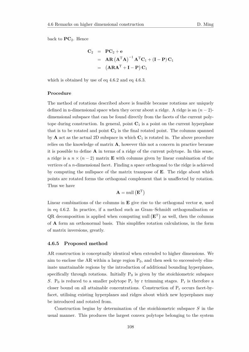
4.6 Remarks on higher dimensional construction D. Ming
back to PC2. Hence
C2 = PC2 + e= AR
(ATA
)−1 ATC1 + (I − P)C1
=(ARAT + I − P
)C1
which is obtained by use of eq 4.6.2 and eq 4.6.3.
Procedure
The method of rotations described above is feasible because rotations are uniquelydefined in n-dimensional space when they occur about a ridge. A ridge is an (n− 2)-dimensional subspace that can be found directly from the facets of the current poly-tope during construction. In general, point C1 is a point on the current hyperplanethat is to be rotated and point C2 is the final rotated point. The columns spannedby A act as the actual 2D subspace in which C1 is rotated in. The above procedurerelies on the knowledge of matrix A, however this not a concern in practice becauseit is possible to define A in terms of a ridge of the current polytope. In this sense,a ridge is a n × (n− 2) matrix E with columns given by linear combination of thevertices of a n-dimensional facet. Finding a space orthogonal to the ridge is achievedby computing the nullspace of the matrix transpose of E. The ridge about whichpoints are rotated forms the orthogonal complement that is unaffected by rotation.Thus we have
A = null(ET)
Linear combinations of the columns in E give rise to the orthogonal vector e, usedin eq 4.6.2. In practice, if a method such as Gram–Schmidt orthogonalisation orQR decomposition is applied when computing null
(ET) as well, then the columns
of A form an orthonormal basis. This simplifies rotation calculations, in the formof matrix inversions, greatly.
4.6.5 Proposed method
AR construction is conceptually identical when extended to higher dimensions. Weaim to enclose the AR within a large region P0, and then seek to successively elim-inate unattainable regions by the introduction of additional bounding hyperplanes,specifically through rotations. Initially P0 is given by the stoichiometric subspaceS. P0 is reduced to a smaller polytope Pr by r trimming stages. Pr is therefore acloser bound on all attainable concentrations. Construction of Pr occurs facet-by-facet, utilising existing hyperplanes and ridges about which new hyperplanes maybe introduced and rotated from.
Construction begins by determination of the stoichiometric subspace S in theusual manner. This produces the largest convex polytope belonging to the system
108
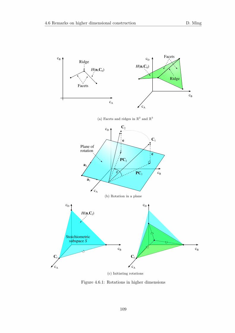
4.6 Remarks on higher dimensional construction D. Ming
cA
cB
cB
cA
cDRidge
FacetsRidge
Facets
H(n,C0)H(n,C0)
(a) Facets and ridges in R2 and R3
e
e C1
C2
cB
cA
cD
PC1
PC2
a1
a2
Plane ofrotation
(b) Rotation in a plane
cB
cA
cD
cB
cA
cD
Cf Cf
H(n,Cf)
Stoichiometricsubspace S
(c) Initiating rotations
Figure 4.6.1: Rotations in higher dimensions
109
4.6 Remarks on higher dimensional construction D. Ming
under consideration, and is the simplest approximation of the AR (S represents allconcentrations satisfying mass balance constraints). The extreme points belongingto S are determined so that the facets and ridges associated with the region maybe constructed. The orientation of a facet in Rn provides an initial orientation ofthe new bounding plane, whilst the ridges of the face provide an orthogonal spaceabout which rotations may be achieved.
Additional hyperplanes are aligned to an existing facet and rotated around theridges associated with the facet. For a problem residing in Rd then, d points must beknown before a facet may be determined. It follows that d possible edges belongingto the face may be chosen for rotations.
The first elimination stage begins by identifying a face passing through the feedpoint Cf which is used to orientate the first bounding hyperplane. The hyperplaneis rotated until a tangent rate vector lying in H (n,Cf) is found, at which pointthe position in space is recorded and a new face is constructed from the remainingd−1 points. In general, hyperplane discretisation and tangency evaluation are easilyextended to higher dimensions. These functions of the elimination step follow untilone of the stopping criteria detailed in section 4.3.1 are met. Creating of a new facetestablishes an orientation for the next hyperplane rotation, whilst a new rotationedge is obtained from the establishment of further edges belonging to the new facet.This is shown in Figure 4.6.1c. The identification of a new vertex in the plane allowsfor the introduction of additional ridges connected to that point. A choice must bemade as to which ridge to utilise next for subsequent rotations, and also a directionof rotation must be specified. These decisions must also take into consideration thefollowing movement criteria:
1. Rotations must not exclude feed or equilibrium points.
2. Rotations may not result in an increase in the size of the feasible region.
After each successive elimination steps, a new facet, or potentially many facets, ofa smaller convex polytope is determined. Nevertheless, selection criteria must bemade established to determine which facet to rotate next. Construction continuesuntil no further rotations are achievable to within a specified tolerance.
Initially, only feed points are known to be achievable and construction of thefirst face is determined by computing the initial extreme points of S. From section4.3.1, the tangency condition exists only to remove unattainable states from theregion; there is no assumption that the tangent point is achievable. Therefore,tangent points that are found from rotations may not, in general, be satisfied byeq 2.3.2. These points may not be physically achievable in a steady state reactornetwork as a consequence. Be that as is may, so long as it is possible to continueintroducing hyperplanes and rotating them into the region, then unachievable statescan be removed from the the set. In Figure 4.6.2, we demonstrate this with a samplepolytope. The region shown in Figure 4.6.2a represents an intermediate polytope
110
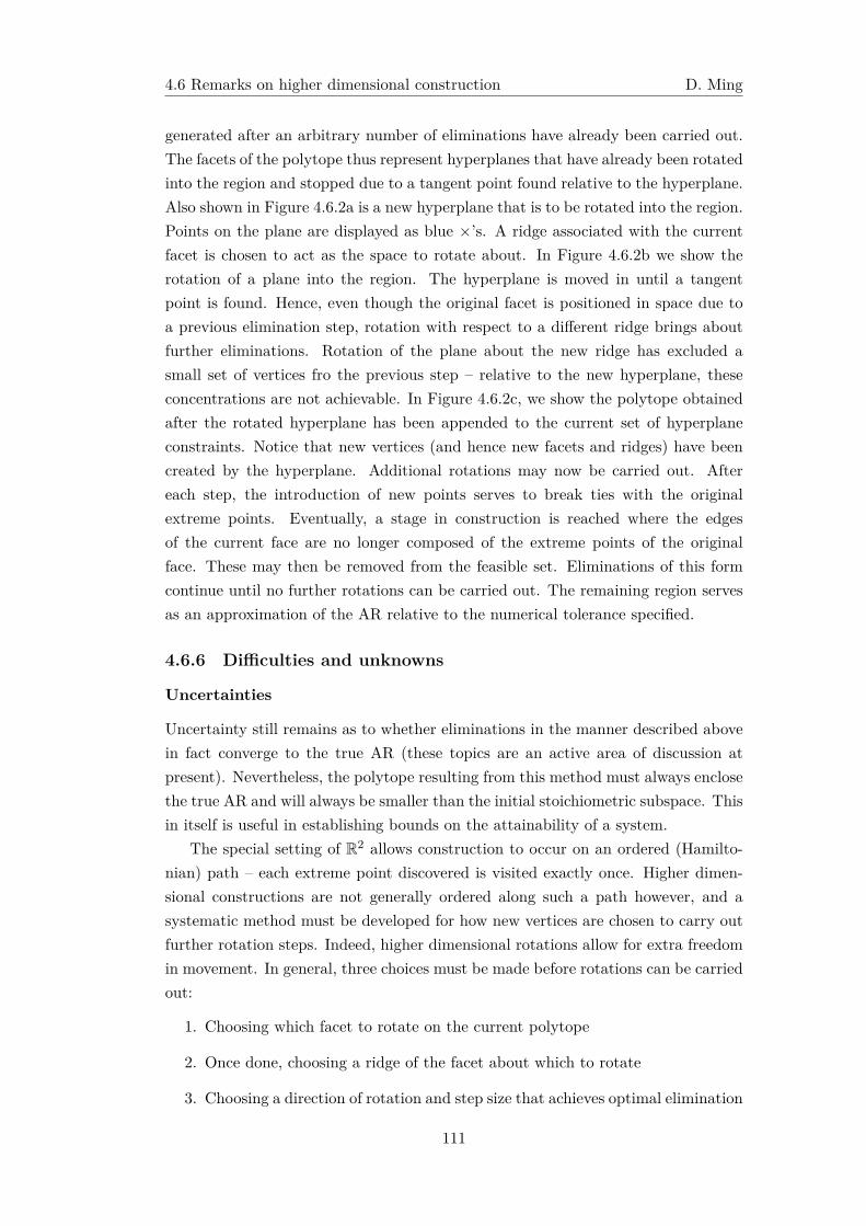
4.6 Remarks on higher dimensional construction D. Ming
generated after an arbitrary number of eliminations have already been carried out.The facets of the polytope thus represent hyperplanes that have already been rotatedinto the region and stopped due to a tangent point found relative to the hyperplane.Also shown in Figure 4.6.2a is a new hyperplane that is to be rotated into the region.Points on the plane are displayed as blue ×’s. A ridge associated with the currentfacet is chosen to act as the space to rotate about. In Figure 4.6.2b we show therotation of a plane into the region. The hyperplane is moved in until a tangentpoint is found. Hence, even though the original facet is positioned in space due toa previous elimination step, rotation with respect to a different ridge brings aboutfurther eliminations. Rotation of the plane about the new ridge has excluded asmall set of vertices fro the previous step – relative to the new hyperplane, theseconcentrations are not achievable. In Figure 4.6.2c, we show the polytope obtainedafter the rotated hyperplane has been appended to the current set of hyperplaneconstraints. Notice that new vertices (and hence new facets and ridges) have beencreated by the hyperplane. Additional rotations may now be carried out. Aftereach step, the introduction of new points serves to break ties with the originalextreme points. Eventually, a stage in construction is reached where the edgesof the current face are no longer composed of the extreme points of the originalface. These may then be removed from the feasible set. Eliminations of this formcontinue until no further rotations can be carried out. The remaining region servesas an approximation of the AR relative to the numerical tolerance specified.
4.6.6 Difficulties and unknowns
Uncertainties
Uncertainty still remains as to whether eliminations in the manner described abovein fact converge to the true AR (these topics are an active area of discussion atpresent). Nevertheless, the polytope resulting from this method must always enclosethe true AR and will always be smaller than the initial stoichiometric subspace. Thisin itself is useful in establishing bounds on the attainability of a system.
The special setting of R2 allows construction to occur on an ordered (Hamilto-nian) path – each extreme point discovered is visited exactly once. Higher dimen-sional constructions are not generally ordered along such a path however, and asystematic method must be developed for how new vertices are chosen to carry outfurther rotation steps. Indeed, higher dimensional rotations allow for extra freedomin movement. In general, three choices must be made before rotations can be carriedout:
1. Choosing which facet to rotate on the current polytope
2. Once done, choosing a ridge of the facet about which to rotate
3. Choosing a direction of rotation and step size that achieves optimal elimination
111
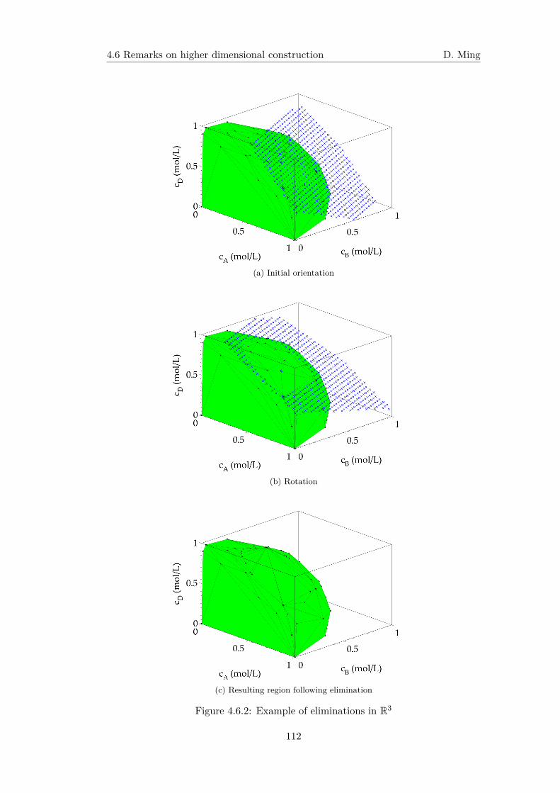
4.6 Remarks on higher dimensional construction D. Ming
(a) Initial orientation
(b) Rotation
(c) Resulting region following elimination
Figure 4.6.2: Example of eliminations in R3
112
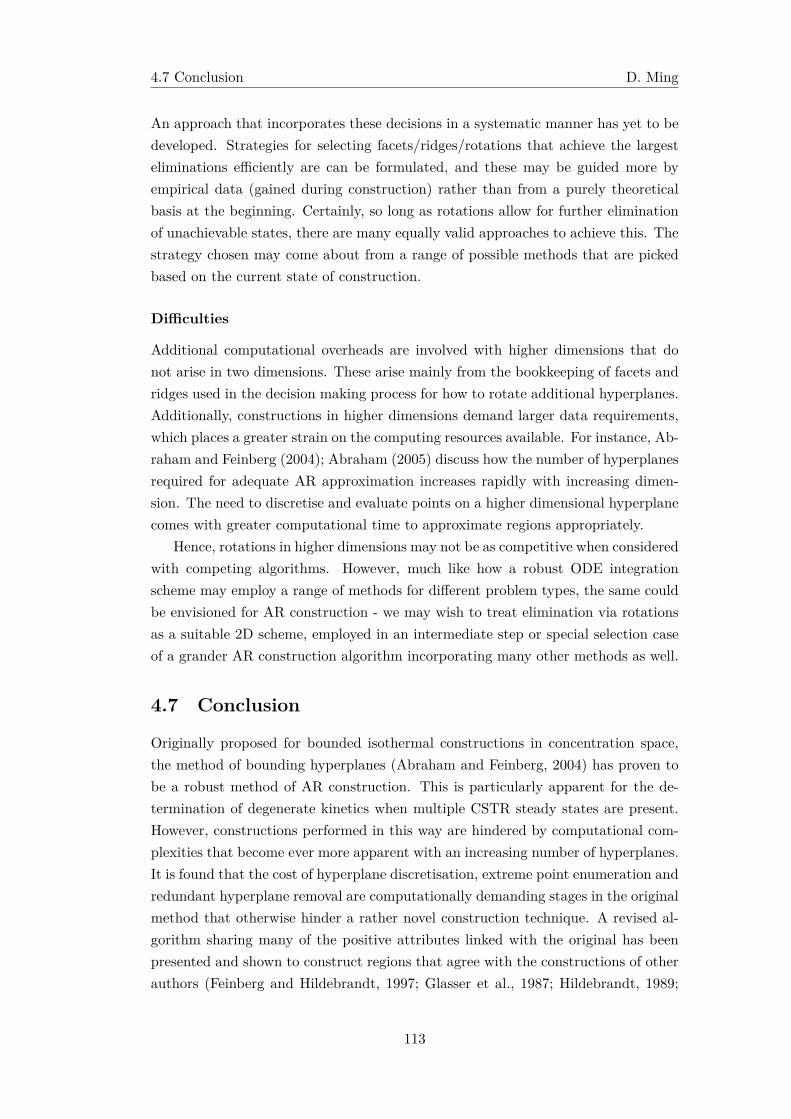
4.7 Conclusion D. Ming
An approach that incorporates these decisions in a systematic manner has yet to bedeveloped. Strategies for selecting facets/ridges/rotations that achieve the largesteliminations efficiently are can be formulated, and these may be guided more byempirical data (gained during construction) rather than from a purely theoreticalbasis at the beginning. Certainly, so long as rotations allow for further eliminationof unachievable states, there are many equally valid approaches to achieve this. Thestrategy chosen may come about from a range of possible methods that are pickedbased on the current state of construction.
Difficulties
Additional computational overheads are involved with higher dimensions that donot arise in two dimensions. These arise mainly from the bookkeeping of facets andridges used in the decision making process for how to rotate additional hyperplanes.Additionally, constructions in higher dimensions demand larger data requirements,which places a greater strain on the computing resources available. For instance, Ab-raham and Feinberg (2004); Abraham (2005) discuss how the number of hyperplanesrequired for adequate AR approximation increases rapidly with increasing dimen-sion. The need to discretise and evaluate points on a higher dimensional hyperplanecomes with greater computational time to approximate regions appropriately.
Hence, rotations in higher dimensions may not be as competitive when consideredwith competing algorithms. However, much like how a robust ODE integrationscheme may employ a range of methods for different problem types, the same couldbe envisioned for AR construction - we may wish to treat elimination via rotationsas a suitable 2D scheme, employed in an intermediate step or special selection caseof a grander AR construction algorithm incorporating many other methods as well.
4.7 Conclusion
Originally proposed for bounded isothermal constructions in concentration space,the method of bounding hyperplanes (Abraham and Feinberg, 2004) has proven tobe a robust method of AR construction. This is particularly apparent for the de-termination of degenerate kinetics when multiple CSTR steady states are present.However, constructions performed in this way are hindered by computational com-plexities that become ever more apparent with an increasing number of hyperplanes.It is found that the cost of hyperplane discretisation, extreme point enumeration andredundant hyperplane removal are computationally demanding stages in the originalmethod that otherwise hinder a rather novel construction technique. A revised al-gorithm sharing many of the positive attributes linked with the original has beenpresented and shown to construct regions that agree with the constructions of otherauthors (Feinberg and Hildebrandt, 1997; Glasser et al., 1987; Hildebrandt, 1989;
113
4.7 Conclusion D. Ming
Seodigeng et al., 2009; Abraham and Feinberg, 2004; Godorr et al., 1999).In much the same way as its predecessor, the method relies on the successive
addition of bounding hyperplanes to separate a region (containing both achievableand unachievable parts) into two half spaces, such that one half contains unattain-able concentrations only. Orientation of the cutting plane has been revised to allowfor a rotation about an axis, rather than a fixed orientation and translation throughspace. This allows for the same trimming mechanism found desirable in the ori-ginal approach, whilst simultaneously eliminating the need for vertex enumerationand redundant hyperplane removal after the introduction of each elimination stage.The method demonstrates an improvement in both running time and constructionaccuracy when compared to the original for the same problem, however the mostgains are observed for kinetics where the AR boundary is composed of many hyper-planes. This might arise when curvature is introduced by PFR solution trajectoriesfor example. These situations involve a large overhead in costly vertex enumerationstages. Construction via rotations of a plane has allowed for the approximation ofunbounded ARs in concentration–time space. The method has also been extendedto allow for determination of non-isothermal ARs and shown to agree with the re-gions obtained via traditional methods. Extension of the method for the inclusionof these cases has allowed for the determination of a rather more broad set of re-actor network optimisation problems that occur frequently in many common reactordesigns.
A discussion of how the algorithm may be extended to n-dimensions was alsopresented. The ideas that characterise construction in R2 take on familiar roles in Rn.Extreme points of existing facets provide starting orientations (positions in space)whilst the edges of the same facet provide an edge about which the bounding planemay be rotated. Eliminations performed in this way allow for the creation of newfacets and edges, about which new hyperplanes may be introduced and rotated tofurther advance the elimination process. Higher dimensional constructions are not assimple to perform as those determined in two dimensions unfortunately. Discussionsas to how these methods may be improved are still actively being investigated. Thisis in part due to the need for additional bookkeeping of facets and edges, but chieflydue to tangent points that are not generally guaranteed to be achievable.
Nevertheless, the performance gain and extended flexibility afforded by non-isothermal and unbounded constructions can now be used in a wider range of reactornetwork problems. It has already been discussed previously how the AR has observeda small adoption in batch. In the next chapter, we will provide simple transforma-tion guidelines for converting continuous reactor structures, used in traditional ARtheory, so that they may be applied to batch directly. We will apply the methoddescribed in this chapter to assist in determining the correct AR boundary belongingto a particular set of kinetics in which multiple steady states occur. These kineticswould otherwise be difficult for traditional inside-out AR construction schemes to
114
References D. Ming
perform. As a result, direct application of the transformation rules from continuousto batch may result in sub-optimal results if the incorrect boundary structure isemployed. The rotated hyperplanes construction method developed in this chapterthus provides a sanity check on the AR. This allows for greater confidence in therecommendations that are obtained from it.
References
Abraham, T. K., 2005. Kinetic bounds on attainability in the reactor synthesisproblem. Ph.D. thesis, Ohio State University, Ohio.
Abraham, T. K., Feinberg, M., 2004. Kinetic bounds on attainability in the reactorsynthesis problem. Industrial & Engineering Chemistry Research 43 (2), 449–457.
Aguilera, A., Perez-Aguila, R., 2004. General n-dimensional rotations. InternationalConference in Central Europe on Computer Graphics, Visualization and ComputerVision.
Burri, J. F., Wilson, S. D., Manousiouthakis, V. I., 2002. Infinite dimensional state-space approach to reactor network synthesis: Application to attainable regionconstruction. Computers & Chemical Engineering 26 (6), 849–862.
Chand, D. R., Kapur, S. S., 1970. Algorithm for convex polytopes. J Ass ComputMach 17 (1), 78–86.
Clausen, J., 1999. Branch and bound algorithms-principles and examples. Depart-ment of Computer Science, University of Copenhagen, 1–30.
Dyer, M. E., 1983. Complexity of vertex enumeration methods. Mathematics ofOperations Research 8 (3), 381–402.
Feinberg, M., 2000a. Optimal reactor design from a geometric viewpoint - iii. criticalcfstrs. Chemical Engineering Science 55 (17), 3553–3565.
Feinberg, M., 2000b. Optimal reactor design from a geometric viewpoint. part ii.critical sidestream reactors. Chemical Engineering Science 55 (13), 2455–2479.
Feinberg, M., Hildebrandt, D., 1997. Optimal reactor design from a geometricviewpoint- i. universal properties of the attainable region. Chemical EngineeringScience 52 (10), 1637–1665.
Glasser, D., Hildebrandt, D., Crowe, C., 1987. A geometric approach to steady flowreactors: The attainable region and optimization in concentration space. Industrial& Engineering Chemistry Research 26 (9), 1803–1810.
Godorr, S., Hildebrandt, D., Glasser, D., McGregor, C., 1999. Choosing optimalcontrol policies using the attainable region approach. Industrial & EngineeringChemistry Research 38 (3), 639–651.
Hildebrandt, D., October 1989. The attainable region generated by reaction andmixing. Ph.D. thesis, University of the Witwatersrand, Johannesburg.
Hildebrandt, D., Glasser, D., 1990. The attainable region and optimal reactor struc-tures. Chemical Engineering Science 45 (8), 2161–2168.
115
References D. Ming
Horn, F., 1964. Attainable and non-attainable regions in chemical reaction tech-nique. Pergamon Press, London.
Kauchali, S., Rooney, W. C., Biegler, L. T., Glasser, D., Hildebrandt, D., 2002.Linear programming formulations for attainable region analysis. Chemical Engin-eering Science 57 (11), 2015–2028.
Land, A. H., Doig, A. G., 1960. An automatic method of solving discrete program-ming problems. Econometrica: Journal of the Econometric Society, 497–520.
Manousiouthakis, V. I., Justanieah, A. M., Taylor, L. A., 2004. The shrink-wrapalgorithm for the construction of the attainable region: An application of theideas framework. Computers & Chemical Engineering 28 (9), 1563–1575.
Nicol, W., Hernier, M., Hildebrant, D., Glasser, D., 2001. The attainable region andprocess synthesis: Reaction systems with external cooling and heating. the effectof relative cost of reactor volume to heat exchange area on the optimal processlayout. Chemical Engineering Science 56 (1), 173–191.
Rooney, W. C., Hausberger, B. P., Biegler, L. T., Glasser, D., 2000. Convex at-tainable region projections for reactor network synthesis. Computers & ChemicalEngineering 24 (2-7), 225–229.
Ryoo, H. S., Sahinidis, N. V., 1995. Global optimization of nonconvex nlps andminlps with applications in process design. Computers & Chemical Engineering19 (5), 551–566.
Schlosser, P. M., Feinberg, M., 1994. A theory of multiple steady states in isothermalhomogeneous cfstrs with many reactions. Chemical Engineering Science 49 (11),1749–1767.
Seodigeng, T., Hausberger, B., Hildebrandt, D., Glasser, D., 2009. Recursive con-stant control policy algorithm for attainable regions analysis. Computers & Chem-ical Engineering 33 (1), 309–320.
Seodigeng, T. G., January 2006. Numerical formulations for attainable region ana-lysis. Ph.D. thesis, University of the Witwatersrand, Johannesburg.
Smith, E. M., Pantelides, C. C., 1999. A symbolic reformulation/spatial branch-and-bound algorithm for the global optimisation of nonconvex minlps. Computers &Chemical Engineering 23 (4), 457–478.
Smith, E. M. d. B., 1996. On the optimal design of continuous processes. Ph.D.thesis, Imperial College London (University of London).
Tawarmalani, M., Sahinidis, N. V., 2004. Global optimization of mixed-integer non-linear programs: A theoretical and computational study. Mathematical program-ming 99 (3), 563–591.
116
Chapter 5
Applying AR theory to batchreactors
The following chapter has been adapted from published work with permission. Theassociated paper is (Ming, D., Glasser, D., Hildebrandt, D., 2013. Application ofAttainable Region theory to batch reactors. Chem. Eng. Sci. 99, 203 – 214.)Copyright (2013) Elsevier. D. Ming (the present author) compiled the manuscriptand contributed to the ideas in this work. D. Hildebrandt and D. Glasser supervisedthis work.
5.1 Introduction
The problem of determining optimal operating policies in batch operations is a pop-ular one, and has been given a great deal of attention in the literature, particularlydue to the importance of batch reaction in a large number of industrially relevantprocesses. Batch reactors are used extensively in the production of a variety of phar-maceutical (Davies and Gloor, 1971) and biological (Cheong et al., 2007; Modak andLim, 1992; Najafpour et al., 2004; Senthuran et al., 1997) products, as well as in thewaste water (Woolard and Irvine, 1995; Zwiener et al., 2002) and polymerisation(Zeman and Amundson, 1965) industries, and are typically considered to be rathermore versatile than that of equivalent continuous processes (Bonvin, 1998). Batchreactors also find use in the small-scale production of highly specialised products,negating the benefit otherwise obtained by large-scale production. Moreover, batchreaction may be the only viable method of producing certain products, such as whenexperimental work is performed at lab-scale and pilot-scale.
It follows that optimisation plays an important function in the design and op-eration of these processes. Much attention has been placed on the development ofmethods that seek to improve batch performance, particularly with regards to thedetermination of optimal operating conditions and scheduling strategies. Althoughresearch into determining efficient batch structures exists (Allgor et al., 1996; Aziz
117
5.2 Overview of AR theory in continuous equipment D. Ming
and Mujtaba, 2002; Capon-Garcia et al., 2011; Mendez et al., 2006), a brief search ofthe current literature would suggest that this area may not appear to be as popularas traditional batch optimisation. Even then, current methods for determining op-timal batch structures often rely on traditional optimisation methods (Allgor et al.,1996, 1999; Allgor and Barton, 1999).
For the past two decades, the papers of Feinberg and Hildebrandt (1997); Fein-berg (1999, 2000b,a); Glasser et al. (1987); Glasser and Hildebrandt (1997) havemotivated the use of a novel method of identifying optimal reactor configurations,termed Attainable Region (AR) analysis. Determination of optimal reactor struc-tures using the AR is unique since synthesis is achieved via a geometric interpretationof reactor configurations. This approach has shown to be an effective alternativemethod to optimal reactor synthesis, particularly with regard to systems involvingmultiple side reactions or reactions with complicated kinetics. Nearly all applica-tions of the AR have been performed on continuous reactors however; the singlepaper of Davis et al. (2008) currently remains the only use of AR theory to batchsystems.
Our aim in this work will thus be towards improving batch reactor structureswith specific use of the AR and the associated benefits of this approach. This isdone as follows: for a given set of feed conditions and kinetics, a candidate ARmay be generated and interpreted, initially, in the form of a continuous reactorstructure. Once generated, the appropriate conversions to the batch setting may beperformed, providing an equivalent recommended batch reactor structure. A keyobjective in this work has been towards reusing the results and insight discoveredfrom a continuous AR structure, such that the same outputs might be obtained withan equivalent batch system.
We will begin by first providing a brief overview of AR theory, and drawing arelevant set of results associated with continuous equipment; this is done in section5.2. Section 5.3 investigates how equivalent structures in batch may be derived fromcontinuous equipment. The correct choice and exact combination of continuousequipment is guided by AR analysis, and thus the development of the AR is centralto the approach presented in this work. Finally, examples and concluding remarksare given in sections 5.4 and 5.5 respectively.
5.2 Overview of AR theory in continuous equipment
5.2.1 AR construction from three fundamental reactor types
The purpose of this section will be towards providing a brief overview of AR theoryfor continuous equipment. The results obtained will allow for the development ofoptimal batch structures. The geometric nature of AR theory has been discussedin numerous papers before Davis et al. (2008); Feinberg and Hildebrandt (1997);
118
5.2 Overview of AR theory in continuous equipment D. Ming
Feinberg (1999, 2000a,b); Glasser et al. (1987); Glasser and Hildebrandt (1997);Godorr et al. (1994, 1999); Hildebrandt and Glasser (1990); Hildebrandt et al. (1990);Khumalo et al. (2006); Nicol et al. (1997, 2001); Nisoli et al. (1997), and only a briefoverview of the theory shall be provided here as a result.
Certain common aspects relating to reaction and mixing were also given treat-ment in chapter 2, and so they are not discussed here either. We do however, wishto repeat certain concepts relating to fundamental reactor types. This will be doneso that comparisons from continuous to batch can be performed directly withoutthe reader needing to constantly refer back to chapter 2. We shall thus begin with abasic review of fundamental reactor types, after which, important properties of theAR boundary will be discussed.
Plug Flow Reactor (PFR)
It may be shown that no more than three fundamental reactor types, togetherwith mixing between structures, are needed to construct the AR (Feinberg andHildebrandt, 1997). These are the plug flow reactor (PFR), the continuously stirredtank reactor (CSTR) and the differential side-stream reactor (DSR). PFRs aredefined by the following expression
dCdτ = r (C) (5.2.1)
Geometrically, the set of concentrations achieved by integration of eq 5.2.1 producesa solution trajectory in concentration space. All rate vectors evaluated along thistrajectory are tangent to it, and thus PFR solutions move along in the direction ofthe vector field. It is shown (Feinberg and Hildebrandt, 1997) that PFR trajectoriesserve to act as highways to which the final most states of the AR boundary areachieved and therefore they assume an important role in the overall optimal ARstructure. In view of this, we find that optimal AR structures usually terminatein a PFR. PFRs allow one to traverse along the outer most extremities of the ARboundary, and as a result, play an integral role in optimal AR structures. A col-lection of PFR trajectories that form part of the AR boundary is often termed amanifold (Feinberg and Hildebrandt, 1997).
Continuously-Stirred Tank Reactor (CSTR)
The CSTR is one in which the reactor contents is assumed to be perfectly mixed,and therefore the exit stream of a CSTR is assumed to be identical to that foundinside the reactor. The defining equation is given as
C = Cf + τr (C) (5.2.2)
119
5.2 Overview of AR theory in continuous equipment D. Ming
CSTRs possess a unique geometric interpretation. If the mixing vector is takenas C − Cf, then clearly the set of concentrations satisfying eq 5.2.2 must be thosepoints which are collinear to r (C). Whereas trajectories corresponding to the PFRare obtained by integration of eq 5.2.1, the locus of points associated with theCSTR are generally found by the solution of a system of non-linear equations. TheCSTR therefore operates on discrete points in space, and hence there exists anopportunity for jumps and discontinuities to also occur as a result. Interpretationof CSTR behaviour in this manner allows for a convenient geometric method forthe determination of CSTR solutions. This is useful for systems involving multiplesteady states. Critical CSTR points are those which reside on the AR boundary.
Differential Side-stream Reactor (DSR)
A DSR may be viewed as a PFR with side-stream addition along its length. Therate of material addition, α, as well as the concentration of the side-stream, C0, areallowed to vary along the reactor length. We will assume that C0 remains at a fixedvalue in this work however.
dCdτ = r (C) + α (C) (C0 − C) (5.2.3)
where 0 ≤ α ≤ ∞. Geometrically, the rate of formation of species achieved in a DSRis determined by the rate of reaction and the mixing vector (C0 − C). The resultantvector is then a linear combination of the two, and the net direction must thereforelie within the space spanned by r (C) and (C0 − C). The overall direction maybe steered between the two by appropriate manipulation of the α parameter, andconsequently, its magnitude must be varied in a manner that produces a trajectorythat is able to maximise the set of achievable concentrations. The unique α policythat allows the DSR trajectory to traverse along the AR boundary is termed acritical α policy, whilst the DSR corresponding to this policy is termed a criticalDSR.
Construction of the AR using structures containing DSRs is only useful for sys-tems involving three or more independent reactions, and thus it is sufficient todescribe the AR, involving two or one independent reactions, with combinations ofPFRs and CSTRs only. It follows that systems with two simultaneous competingreactions may be solved without the use of DSRs.
5.2.2 Necessary conditions of the AR
From the above discussion, it is possible to establish a set of necessary conditionsthat the AR must satisfy (Glasser et al., 1987; Glasser and Hildebrandt, 1997); theseare:
• The AR must contain the feed – The feed point is attainable, and therefore it
120
5.2 Overview of AR theory in continuous equipment D. Ming
must be contained with the set of all achievable points.
• The AR must be convex – A set of achievable points that is not convex canalways be made convex by mixing. Mixing can fill in concave regions andspaces between two separate, yet achievable, regions.
• All rate vectors on the boundary of the AR must point into, or be tangent, tothe AR – A PFR may be used to extend the region otherwise.
• All rate vectors (or linear combinations of rate vectors) located in the com-pliment of the AR may not be extended backwards to intersect the boundary– A CSTR may be used to achieve the given point and therefore extend theregion otherwise.
Currently, there exists no sufficiency condition for the AR. Regions that are producedthat satisfy the above necessary conditions are therefore termed candidate attainableregions. A number of AR construction methods, suitable for implementation oncomputer, have been devised. The interested reader should refer to the works ofRooney et al. (2000); Burri et al. (2002); Kauchali et al. (2002); Abraham andFeinberg (2004); Manousiouthakis et al. (2004); Zhou and Manousiouthakis (2006);Seodigeng et al. (2009); Ming et al. (2010) for further details.
5.2.3 Dimensional considerations
Dimension of the AR
Although it is natural to describe the dimension of the AR in terms of the totalnumber of species in the system, these are generally not independent, and hencethis approach may be unnecessary. Feinberg (2000b,a) demonstrated that it is usu-ally possible to recast the AR in a lower dimensional subspace in RL. Here, L is thenumber of linearly independent reactions taking part in the system. In addition tothis, given an initial feed concentration and system stoichiometry, the set of attain-able compositions achieved by reaction and mixing may not violate the conservationof mass. The AR must therefore be bounded by stoichiometric constraints. This re-gion is termed the stoichiometric subspace. We denote by S the set of concentrationsstoichiometrically compatible with the feed.
Maximum number of parallel structures
There also exists an upper bound on the maximum number of parallel structuresrequired by the AR in order to achieve a given state. These bounds hold for bothwithin the AR, and on its boundary (Feinberg, 2000b), and are a consequence ofCarathéodory’s theorem. The results are summarised below for an AR constructedin Rn:
121
5.3 Similarities between batch and continuous reactive equipment D. Ming
• The maximum number of parallel structures required to achieve any concen-tration within the interior of the region is n.
• If concentrations on the boundary are to be achieved, the number of parallelstructures is, at most, equal to n− 1.
It follows that the maximum number of parallel structures is equal to the numberof independent reactions in the system. Although it is generally not possible todetermine, a priori, the number or sequence of reactor units that make up a branchof an optimal AR structure, it is still feasible to obtain an upper bound on themaximum number of unique parallel structures required by the system. Unless theobjective function intersects the AR boundary at multiple points, it is generally nota requirement that all optimal reactor structures be used in the optimisation. Thisresult shall become more meaningful in the examples that are to follow.
5.3 Similarities between batch and continuous reactiveequipment
A note on continuous and batch operation
In the upcoming discussion, we will want to show how the states realized in thethree fundamental continuous reactors used in AR theory can be achieved by batchequipment. Moreover, we would like to demonstrate that the necessary transform-ations from continuous to batch can be used in conjunction with the AR to helpguide the design of optimal batch structures. Before we begin our discussion onthe similarities between batch and continuous reactors however, we would like tohighlight a clear difference between the two operating regimes.
Thus, even though we wish to show that it is possible to attain steady stateconcentrations in a batch, it is not assumed that steady state itself can ever beattained. By the very nature of batch processes, this is clearly not possible. Hence,our outlook here will not be of the view that batch reactors, specifically fed-batchreactors, can ever be operated in any particular way that is able to reach steady state.We would, however, like to demonstrate that it is still possible to achieve the specificconcentration associated with that steady state. Certainly, this will require a specialoperating regime to achieve (which shall be detailed in the following sections), butthis will always be with the idea that the reactor is operated under batch conditions- that is, with a distinct cycle time in which the state variables of the batch reactor(volume, concentration, etc.) do, in fact, vary for the duration of this period. Withthis in mind, let us begin our discussion starting with the simplest of cases.
122
5.3 Similarities between batch and continuous reactive equipment D. Ming
5.3.1 The standard batch
By standard batch, we have in mind a batch reactor where there is no inflow oroutflow of material during the reaction period. The reactor contents are well mixed,although, the concentration of species evolves with respect to time. Given an initialconcentration of species, the concentration profile within a standard batch reactormay be determined by integration of the appropriate rate expression. Thus, we havefor the standard batch
dCdt = r (C) (5.3.1)
Thus, the solution trajectory obtained by integration of eq 5.3.1 is identical to thatobtained by integration of eq 5.2.1 for the same initial conditions - the initial con-centration of the standard batch at t = 0 is identical to the feed concentration in aPFR at τ = 0. The reaction time of the batch replaces residence time of the PFRas the integration parameter in this regard. As a result, optimal reactor structureswhere PFRs form the boundary of the AR may be achieved in batch processes byrunning a standard batch reactor with the appropriate reaction time.
5.3.2 Fed-batch reaction
Fed-batch or semi-batch reactors are reactors that allow the feeding of additionalmaterial into the reaction vessel during the reaction period, and may be used tobias the selectivity of components in competing reactions. Assume that a fed-batchreactor is available with a side-stream volumetric feed rate of F (F has units of[volume]/[time]) and a side-stream concentration of C0. It is assumed that F varieswith respect to time whereas the side-stream feed concentration, C0, is constant. Amolar balance for component i over the fed-batch with respect to time results in thefollowing differential equation
dni
dt = V (t) ri (C) + F (t) c0i
where ni, ri (C) and c0i are the moles of i in the reactor, species rate function andside-stream concentration of component i, respectively, ,and V (t) is the currentvolume of the reactor. Expressing ni in terms of ci by ni = ciV (t)gives
cidVdt + V (t) dci
dt = V (t) ri (C) + F (t) c0i
and recognising that a volume balance over the fed-batch
dVdt = F (t)
this results indcidt = ri (C) +
[F (t)V (t)
] (c0i − ci
)123
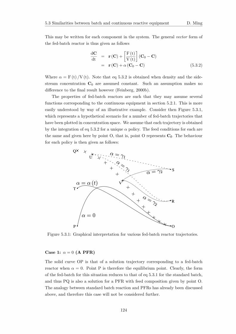
5.3 Similarities between batch and continuous reactive equipment D. Ming
This may be written for each component in the system. The general vector form ofthe fed-batch reactor is thus given as follows
dCdt = r (C) +
[F (t)V (t)
](C0 − C)
= r (C) + α (C0 − C) (5.3.2)
Where α = F (t) /V (t). Note that eq 5.3.2 is obtained when density and the side-stream concentration C0 are assumed constant. Such an assumption makes nodifference to the final result however (Feinberg, 2000b).
The properties of fed-batch reactors are such that they may assume severalfunctions corresponding to the continuous equipment in section 5.2.1. This is moreeasily understood by way of an illustrative example. Consider then Figure 5.3.1,which represents a hypothetical scenario for a number of fed-batch trajectories thathave been plotted in concentration space. We assume that each trajectory is obtainedby the integration of eq 5.3.2 for a unique α policy. The feed conditions for each arethe same and given here by point O, that is, point O represents Cf. The behaviourfor each policy is then given as follows:
Figure 5.3.1: Graphical interpretation for various fed-batch reactor trajectories.
Case 1: α = 0 (A PFR)
The solid curve OP is that of a solution trajectory corresponding to a fed-batchreactor when α = 0. Point P is therefore the equilibrium point. Clearly, the formof the fed-batch for this situation reduces to that of eq 5.3.1 for the standard batch,and thus PQ is also a solution for a PFR with feed composition given by point O.The analogy between standard batch reaction and PFRs has already been discussedabove, and therefore this case will not be considered further.
124
5.3 Similarities between batch and continuous reactive equipment D. Ming
Case 2: α = α (C (t)) (A DSR)
The most familiar method of operation is one in which the feed addition policy isadjusted throughout the reaction period. Hence, consider now the case when α isgiven by a varying profile. Again, eq 5.3.2 may be integrated if an initial condition,side-stream composition (given by C0) and α policy are supplied. The curve OTis representative of such a solution where point T is the equilibrium point for thistrajectory. Observe once more that the form of the fed-batch equation is identicalto eq 5.2.3 for the DSR, and identical behaviour may be achieved in the batch byappropriate interpretation of the α variable as a result.
The set of concentrations belonging to the trajectory OT is thus equivalent tothat obtained in a DSR with feed composition equal to point O, and side-streamcomposition given by C0 (not shown in the figure). With similar reasoning to thestandard batch/PFR analogy, residence time in the DSR is replaced by reaction timein the fed-batch. The value of α in the DSR represents the feed rate with respect toDSR length, whereas in the batch, α = F/V (the ratio of side-stream addition feedrate to reactor volume). F (t) and V (t) are determined by integration of the α policywith respect to time and the differential expression for the volume change, usuallygiven by dV/dt = F (t). Nevertheless, notice that there is a direct analogue betweenfed-batch reactors with varying α policies and DSRs. AR boundary structures thatcontain DSR segments are thus easily convertible to an equivalent fed-batch systemas a result.
Case 3: α = constant (A CSTR)
Consider now the particular case when α is maintained at a constant value through-out the reaction period. Again, if an initial condition and fed-batch addition com-position are specified, eq 5.3.2 can be integrated for any arbitrary reaction time.The pair of curves represented by RU and SU are representative solutions for whenα is kept at a constant value of γ1, whereas the pair RV and SV is that which isobtained when α is kept at a different value given by γ2. Clearly, RU and RV sharethe same initial point, given by point R, and points SU and SV share the sameinitial condition given by S. For α = γ1, the fed-batch trajectories both terminate atpoint U, even though the starting conditions differ, the same behaviour is observedfor α = γ2. All trajectories however (RU, SU, RV and SV), are fed with material ofconcentration given by point O.
For a sufficiently long reaction time, the concentration of species within the vesselapproaches equilibrium, and eq 5.3.2 reduces to
0 = r (C) + α (C0 − C) (5.3.3)
End points U and V therefore represent equilibrium points in the fed-batch for a
125
5.3 Similarities between batch and continuous reactive equipment D. Ming
constant α policy, and are thus also solutions to eq 5.3.3. For all values of α in therange 0 < α < ∞, integration of eq 5.3.2 to equilibrium may be carried out with thefed-batch feed concentration C0 set at point O. The locus of (×) given by the curveOVUQ represents the set of equilibrium concentrations achieved in the system as aresult.
Clearly, equilibrium concentrations for the fed-batch are equivalent to CSTRconcentrations when the CSTR feed composition, Cf, is equal to point O. This maybe more easily seen by comparing eq 5.3.3 to the form of the CSTR expression givenby eq 5.2.2. The value of α at equilibrium is thus related to the CSTR residencetime by
α =1
τCSTRat equilibrium
It follows that all values of α in the range 0 ≤ α ≤ ∞ for fed-batch reactors operatingat equilibrium correspond to the set of CSTRs with residence times between therange ∞ ≤ τCSTR ≤ 0.
The curve OVUQ in Figure 5.3.1 also corresponds to solutions for a CSTR (withfeed point O), and therefore curve OVUQ is also representative of a CSTR locus.CSTR compositions can thus be obtained in a batch by operating a fed-batch reactorat its equilibrium concentration. The particular equilibrium point is defined by thespecific constant α value chosen, which corresponds to a particular CSTR solutionwith residence time given by τ = 1/α.
Several observations may be noted for the constant α fed-batch reactor withrelation to a CSTR:
1. Initial conditions
Notice that the equilibrium point in the fed-batch is defined by the value ofα and the fed-batch feed concentration, and is not a function of the initialcondition at t = 0. The choice of initial condition may still be somewhatconstrained, as certain specific instances prevent the designer from choosingthe starting point in a completely arbitrary manner. Details of these arediscussed under point 3.
It follows that equivalent CSTR behaviour may only be achieved in the fed-batch at equilibrium, and therefore, in order to obtain CSTR concentrationsin a batch system, the reactor must be initiated at the equilibrium conditions.In practice, this may be achieved by several methods:
• Initially run a small CSTR at the appropriate residence time to producethe desired equilibrium composition. Then transfer the contents of theCSTR into a fed-batch.
• Begin at a condition sufficiently close to the desired CSTR concentrationso that equilibrium may be approached during the reaction period.
126
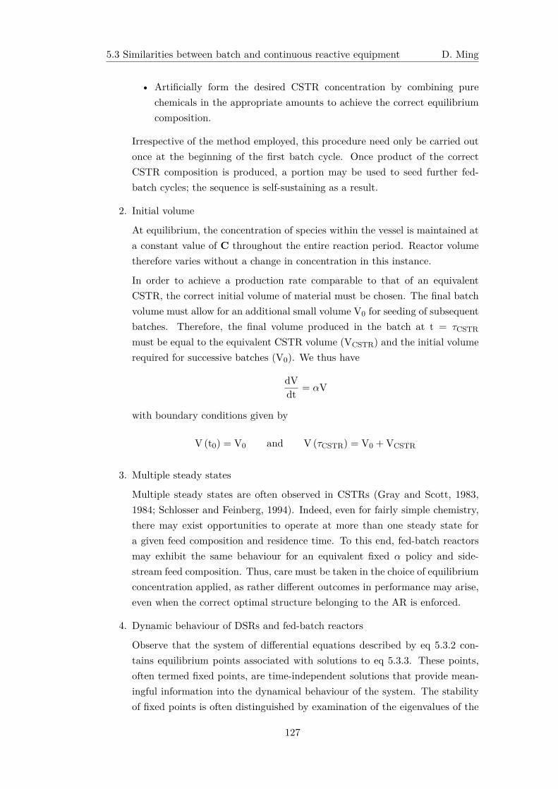
5.3 Similarities between batch and continuous reactive equipment D. Ming
• Artificially form the desired CSTR concentration by combining purechemicals in the appropriate amounts to achieve the correct equilibriumcomposition.
Irrespective of the method employed, this procedure need only be carried outonce at the beginning of the first batch cycle. Once product of the correctCSTR composition is produced, a portion may be used to seed further fed-batch cycles; the sequence is self-sustaining as a result.
2. Initial volume
At equilibrium, the concentration of species within the vessel is maintained ata constant value of C throughout the entire reaction period. Reactor volumetherefore varies without a change in concentration in this instance.
In order to achieve a production rate comparable to that of an equivalentCSTR, the correct initial volume of material must be chosen. The final batchvolume must allow for an additional small volume V0 for seeding of subsequentbatches. Therefore, the final volume produced in the batch at t = τCSTR
must be equal to the equivalent CSTR volume (VCSTR) and the initial volumerequired for successive batches (V0). We thus have
dVdt = αV
with boundary conditions given by
V (t0) = V0 and V (τCSTR) = V0 + VCSTR
3. Multiple steady states
Multiple steady states are often observed in CSTRs (Gray and Scott, 1983,1984; Schlosser and Feinberg, 1994). Indeed, even for fairly simple chemistry,there may exist opportunities to operate at more than one steady state fora given feed composition and residence time. To this end, fed-batch reactorsmay exhibit the same behaviour for an equivalent fixed α policy and side-stream feed composition. Thus, care must be taken in the choice of equilibriumconcentration applied, as rather different outcomes in performance may arise,even when the correct optimal structure belonging to the AR is enforced.
4. Dynamic behaviour of DSRs and fed-batch reactors
Observe that the system of differential equations described by eq 5.3.2 con-tains equilibrium points associated with solutions to eq 5.3.3. These points,often termed fixed points, are time-independent solutions that provide mean-ingful information into the dynamical behaviour of the system. The stabilityof fixed points is often distinguished by examination of the eigenvalues of the
127
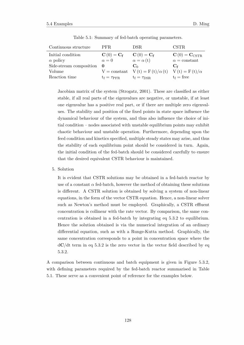
5.4 Examples D. Ming
Table 5.1: Summary of fed-batch operating parameters.
Continuous structure PFR DSR CSTRInitial condition C (0) = Cf C (0) = Cf C (0) = CCSTRα policy α = 0 α = α (t) α = constantSide-stream composition 0 C0 CfVolume V = constant V (t) = F (t)/α (t) V (t) = F (t)/αReaction time tf = τPFR tf = τDSR tf = free
Jacobian matrix of the system (Strogatz, 2001). These are classified as eitherstable, if all real parts of the eigenvalues are negative, or unstable, if at leastone eigenvalue has a positive real part, or if there are multiple zero eigenval-ues. The stability and position of the fixed points in state space influence thedynamical behaviour of the system, and thus also influence the choice of ini-tial condition – nodes associated with unstable equilibrium points may exhibitchaotic behaviour and unstable operation. Furthermore, depending upon thefeed condition and kinetics specified, multiple steady states may arise, and thusthe stability of each equilibrium point should be considered in turn. Again,the initial condition of the fed-batch should be considered carefully to ensurethat the desired equivalent CSTR behaviour is maintained.
5. Solution
It is evident that CSTR solutions may be obtained in a fed-batch reactor byuse of a constant α fed-batch, however the method of obtaining these solutionsis different. A CSTR solution is obtained by solving a system of non-linearequations, in the form of the vector CSTR equation. Hence, a non-linear solversuch as Newton’s method must be employed. Graphically, a CSTR effluentconcentration is collinear with the rate vector. By comparison, the same con-centration is obtained in a fed-batch by integrating eq 5.3.2 to equilibrium.Hence the solution obtained is via the numerical integration of an ordinarydifferential equation, such as with a Runge-Kutta method. Graphically, thesame concentration corresponds to a point in concentration space where thedC/dt term in eq 5.3.2 is the zero vector in the vector field described by eq5.3.2.
A comparison between continuous and batch equipment is given in Figure 5.3.2,with defining parameters required by the fed-batch reactor summarised in Table5.1. These serve as a convenient point of reference for the examples below.
128
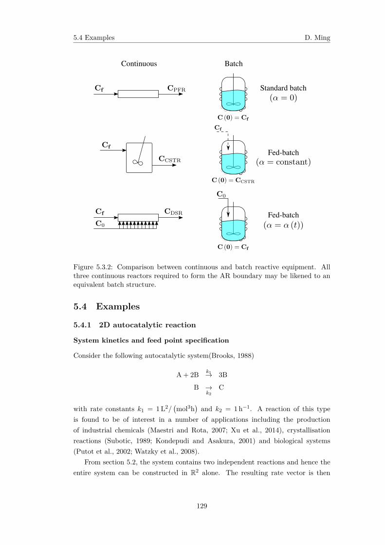
5.4 Examples D. Ming
Continuous Batch
Fed-batch
Standard batch
Fed-batch
Figure 5.3.2: Comparison between continuous and batch reactive equipment. Allthree continuous reactors required to form the AR boundary may be likened to anequivalent batch structure.
5.4 Examples
5.4.1 2D autocatalytic reaction
System kinetics and feed point specification
Consider the following autocatalytic system(Brooks, 1988)
A + 2B k1→ 3B
B →k2
C
with rate constants k1 = 1L2/(mol3h
)and k2 = 1 h−1. A reaction of this type
is found to be of interest in a number of applications including the productionof industrial chemicals (Maestri and Rota, 2007; Xu et al., 2014), crystallisationreactions (Subotic, 1989; Kondepudi and Asakura, 2001) and biological systems(Putot et al., 2002; Watzky et al., 2008).
From section 5.2, the system contains two independent reactions and hence theentire system can be constructed in R2 alone. The resulting rate vector is then
129
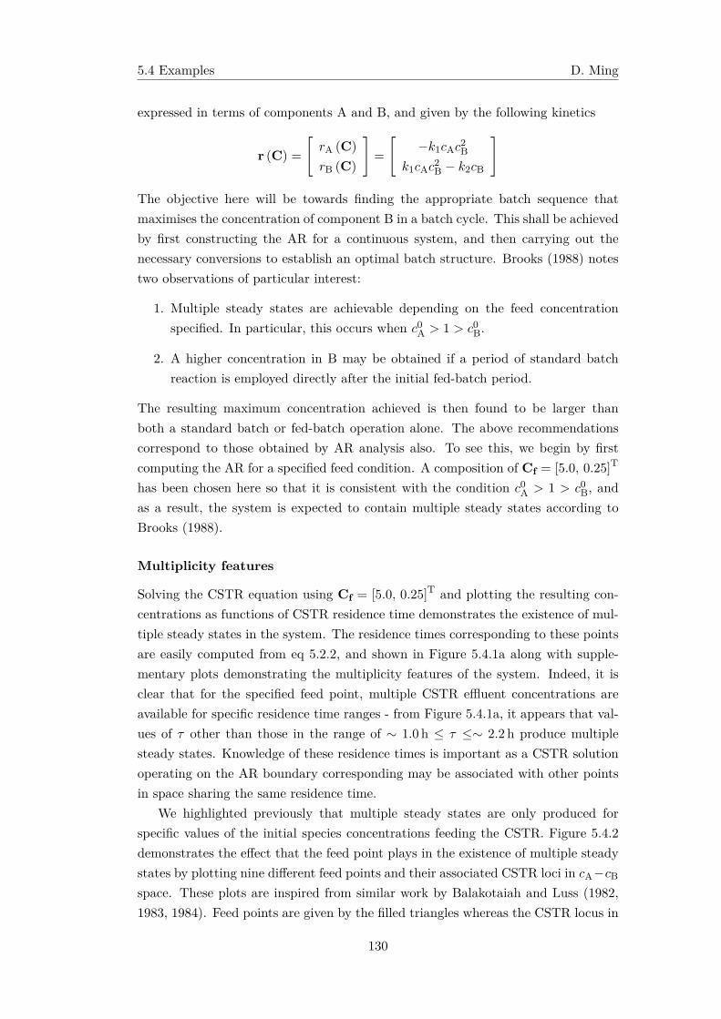
5.4 Examples D. Ming
expressed in terms of components A and B, and given by the following kinetics
r (C) =
[rA (C)
rB (C)
]=
[−k1cAc
2B
k1cAc2B − k2cB
]
The objective here will be towards finding the appropriate batch sequence thatmaximises the concentration of component B in a batch cycle. This shall be achievedby first constructing the AR for a continuous system, and then carrying out thenecessary conversions to establish an optimal batch structure. Brooks (1988) notestwo observations of particular interest:
1. Multiple steady states are achievable depending on the feed concentrationspecified. In particular, this occurs when c0A > 1 > c0B.
2. A higher concentration in B may be obtained if a period of standard batchreaction is employed directly after the initial fed-batch period.
The resulting maximum concentration achieved is then found to be larger thanboth a standard batch or fed-batch operation alone. The above recommendationscorrespond to those obtained by AR analysis also. To see this, we begin by firstcomputing the AR for a specified feed condition. A composition of Cf = [5.0, 0.25]T
has been chosen here so that it is consistent with the condition c0A > 1 > c0B, andas a result, the system is expected to contain multiple steady states according toBrooks (1988).
Multiplicity features
Solving the CSTR equation using Cf = [5.0, 0.25]T and plotting the resulting con-centrations as functions of CSTR residence time demonstrates the existence of mul-tiple steady states in the system. The residence times corresponding to these pointsare easily computed from eq 5.2.2, and shown in Figure 5.4.1a along with supple-mentary plots demonstrating the multiplicity features of the system. Indeed, it isclear that for the specified feed point, multiple CSTR effluent concentrations areavailable for specific residence time ranges - from Figure 5.4.1a, it appears that val-ues of τ other than those in the range of ∼ 1.0 h ≤ τ ≤∼ 2.2h produce multiplesteady states. Knowledge of these residence times is important as a CSTR solutionoperating on the AR boundary corresponding may be associated with other pointsin space sharing the same residence time.
We highlighted previously that multiple steady states are only produced forspecific values of the initial species concentrations feeding the CSTR. Figure 5.4.2demonstrates the effect that the feed point plays in the existence of multiple steadystates by plotting nine different feed points and their associated CSTR loci in cA−cB
space. These plots are inspired from similar work by Balakotaiah and Luss (1982,1983, 1984). Feed points are given by the filled triangles whereas the CSTR locus in
130
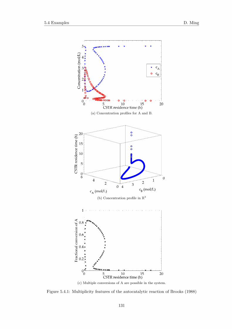
5.4 Examples D. Ming
(a) Concentration profiles for A and B.
(b) Concentration profile in R3
(c) Multiple conversions of A are possible in the system.
Figure 5.4.1: Multiplicity features of the autocatalytic reaction of Brooks (1988)
131
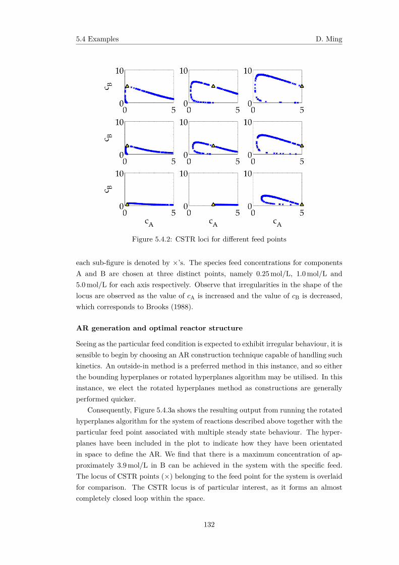
5.4 Examples D. Ming
Figure 5.4.2: CSTR loci for different feed points
each sub-figure is denoted by ×’s. The species feed concentrations for componentsA and B are chosen at three distinct points, namely 0.25mol/L, 1.0mol/L and5.0mol/L for each axis respectively. Observe that irregularities in the shape of thelocus are observed as the value of cA is increased and the value of cB is decreased,which corresponds to Brooks (1988).
AR generation and optimal reactor structure
Seeing as the particular feed condition is expected to exhibit irregular behaviour, it issensible to begin by choosing an AR construction technique capable of handling suchkinetics. An outside-in method is a preferred method in this instance, and so eitherthe bounding hyperplanes or rotated hyperplanes algorithm may be utilised. In thisinstance, we elect the rotated hyperplanes method as constructions are generallyperformed quicker.
Consequently, Figure 5.4.3a shows the resulting output from running the rotatedhyperplanes algorithm for the system of reactions described above together with theparticular feed point associated with multiple steady state behaviour. The hyper-planes have been included in the plot to indicate how they have been orientatedin space to define the AR. We find that there is a maximum concentration of ap-proximately 3.9mol/L in B can be achieved in the system with the specific feed.The locus of CSTR points (×) belonging to the feed point for the system is overlaidfor comparison. The CSTR locus is of particular interest, as it forms an almostcompletely closed loop within the space.
132
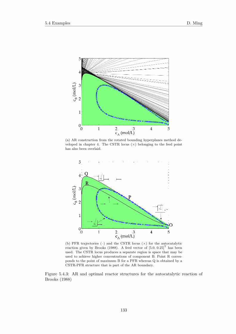
5.4 Examples D. Ming
(a) AR construction from the rotated bounding hyperplanes method de-veloped in chapter 4. The CSTR locus (×) belonging to the feed pointhas also been overlaid.
(b) PFR trajectories (–) and the CSTR locus (×) for the autocatalyticreaction given by Brooks (1988). A feed vector of [5.0, 0.25]T has beenused. The CSTR locus produces a separate region is space that may beused to achieve higher concentrations of component B. Point R corres-ponds to the point of maximum B for a PFR whereas Q is obtained by aCSTR-PFR structure that is part of the AR boundary.
Figure 5.4.3: AR and optimal reactor structures for the autocatalytic reaction ofBrooks (1988)
133
5.4 Examples D. Ming
In Figure 5.4.3b optimal reactor structures, corresponding to interesting sectionsof the AR, are shown. The PFR trajectory and CSTR locus beginning at thefeed point have been plotted. Figure 5.4.3b also establishes all physically realisableconcentrations achieved by mixing and reaction; that is, the shaded region representsthe AR for the chosen feed point. This is obtained by computing the convex hull of allpoints resulting from a CSTR with feed concentration (point O), followed by a PFRto equilibrium. The CSTR-PFR sequence is thus the optimal reactor structure forthe proposed AR. It follows that this is the only structure required in order to achieveall other physically realisable concentrations in the space. Of particular interest ispoint P, which provides the unique CSTR concentration that, when followed by aPFR, maximises the concentration of component B in the system; this occurs atpoint Q (cB ∼ 3.9mol/L). The corresponding CSTR residence time is then found tobe 0.18367h accordingly. Point P therefore corresponds to a critical CSTR point. Allconcentrations on the line segment OP are thus obtained by a CSTR with bypassof a portion of the feed. These results are in agreement with those suggested byBrooks (1988) for the batch case, where it is observed that a higher concentrationin component B may be achieved if a standard batch is employed directly after thefed-batch period. This is displayed in the figure by the PFR trajectory PQ. PointR by comparison, is the point of maximum B for a single PFR initiated at the feedcomposition found at point O.
Nomenclature adopted by Brooks
Brooks (1988) discusses a strategy for reaction by initiating the cycle in fed-batchoperation, and then terminating the cycle by charging the vessel with the remainderof feeding material in the form of a final feeding ‘plug’. This converts the fed-batchinto a standard batch, creating a fed-batch to standard batch reactor structuresimilar to the that obtained by AR analysis. When this is performed, Brooks (1988)notes that the concentration of B is higher than if standard batch operation isemployed for the entire reaction cycle.
In order for comparisons to be made with the current work, a consistent set ofquantities for concentration and reaction time need to be established. Brooks (1988)works with dimensionless concentrations in the form
x =
(k1k2
)1/2
cA y =
(k1k2
)1/2
cB
Note that x = cA and y = cB when k1 = 1L2/(mol3h
)and k2 = 1 hr−1, as is the
case here. Brooks (1988) also assumes the fed-batch is operated under a constantfeeding rate (F = const). A volume balance over a fed-batch assuming constantdensity gives
dVdt = F
134
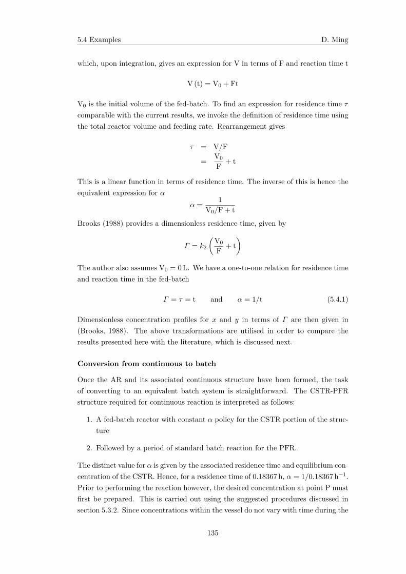
5.4 Examples D. Ming
which, upon integration, gives an expression for V in terms of F and reaction time t
V (t) = V0 + Ft
V0 is the initial volume of the fed-batch. To find an expression for residence time τ
comparable with the current results, we invoke the definition of residence time usingthe total reactor volume and feeding rate. Rearrangement gives
τ = V/F
=V0
F + t
This is a linear function in terms of residence time. The inverse of this is hence theequivalent expression for α
α =1
V0/F + t
Brooks (1988) provides a dimensionless residence time, given by
Γ = k2
(V0
F + t)
The author also assumes V0 = 0L. We have a one-to-one relation for residence timeand reaction time in the fed-batch
Γ = τ = t and α = 1/t (5.4.1)
Dimensionless concentration profiles for x and y in terms of Γ are then given in(Brooks, 1988). The above transformations are utilised in order to compare theresults presented here with the literature, which is discussed next.
Conversion from continuous to batch
Once the AR and its associated continuous structure have been formed, the taskof converting to an equivalent batch system is straightforward. The CSTR-PFRstructure required for continuous reaction is interpreted as follows:
1. A fed-batch reactor with constant α policy for the CSTR portion of the struc-ture
2. Followed by a period of standard batch reaction for the PFR.
The distinct value for α is given by the associated residence time and equilibrium con-centration of the CSTR. Hence, for a residence time of 0.18367h, α = 1/0.18367h−1.Prior to performing the reaction however, the desired concentration at point P mustfirst be prepared. This is carried out using the suggested procedures discussed insection 5.3.2. Since concentrations within the vessel do not vary with time during the
135
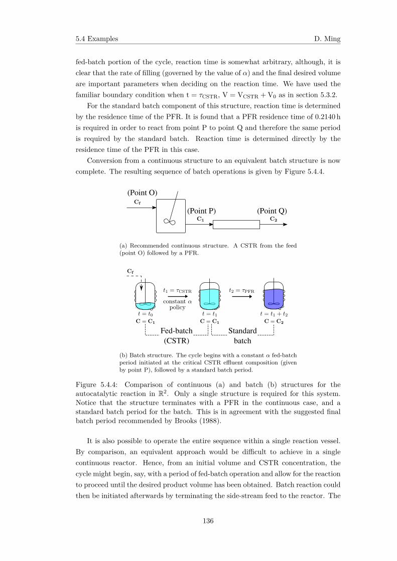
5.4 Examples D. Ming
fed-batch portion of the cycle, reaction time is somewhat arbitrary, although, it isclear that the rate of filling (governed by the value of α) and the final desired volumeare important parameters when deciding on the reaction time. We have used thefamiliar boundary condition when t = τCSTR, V = VCSTR + V0 as in section 5.3.2.
For the standard batch component of this structure, reaction time is determinedby the residence time of the PFR. It is found that a PFR residence time of 0.2140 his required in order to react from point P to point Q and therefore the same periodis required by the standard batch. Reaction time is determined directly by theresidence time of the PFR in this case.
Conversion from a continuous structure to an equivalent batch structure is nowcomplete. The resulting sequence of batch operations is given by Figure 5.4.4.
(Point O)
(Point P) (Point Q)
(a) Recommended continuous structure. A CSTR from the feed(point O) followed by a PFR.
Fed-batch(CSTR)
Standard batch
(b) Batch structure. The cycle begins with a constant α fed-batchperiod initiated at the critical CSTR effluent composition (givenby point P), followed by a standard batch period.
Figure 5.4.4: Comparison of continuous (a) and batch (b) structures for theautocatalytic reaction in R2. Only a single structure is required for this system.Notice that the structure terminates with a PFR in the continuous case, and astandard batch period for the batch. This is in agreement with the suggested finalbatch period recommended by Brooks (1988).
It is also possible to operate the entire sequence within a single reaction vessel.By comparison, an equivalent approach would be difficult to achieve in a singlecontinuous reactor. Hence, from an initial volume and CSTR concentration, thecycle might begin, say, with a period of fed-batch operation and allow for the reactionto proceed until the desired product volume has been obtained. Batch reaction couldthen be initiated afterwards by terminating the side-stream feed to the reactor. The
136
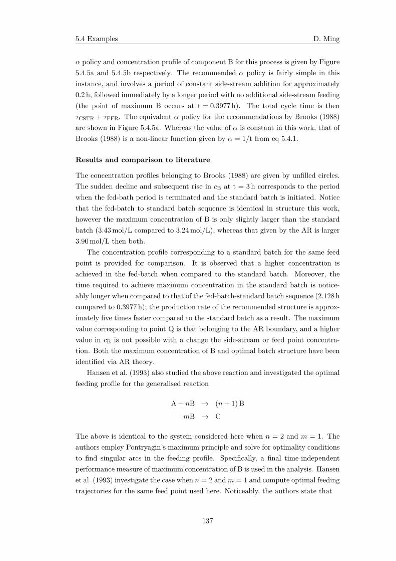
5.4 Examples D. Ming
α policy and concentration profile of component B for this process is given by Figure5.4.5a and 5.4.5b respectively. The recommended α policy is fairly simple in thisinstance, and involves a period of constant side-stream addition for approximately0.2h, followed immediately by a longer period with no additional side-stream feeding(the point of maximum B occurs at t = 0.3977 h). The total cycle time is thenτCSTR + τPFR. The equivalent α policy for the recommendations by Brooks (1988)are shown in Figure 5.4.5a. Whereas the value of α is constant in this work, that ofBrooks (1988) is a non-linear function given by α = 1/t from eq 5.4.1.
Results and comparison to literature
The concentration profiles belonging to Brooks (1988) are given by unfilled circles.The sudden decline and subsequent rise in cB at t = 3 h corresponds to the periodwhen the fed-bath period is terminated and the standard batch is initiated. Noticethat the fed-batch to standard batch sequence is identical in structure this work,however the maximum concentration of B is only slightly larger than the standardbatch (3.43mol/L compared to 3.24mol/L), whereas that given by the AR is larger3.90mol/L then both.
The concentration profile corresponding to a standard batch for the same feedpoint is provided for comparison. It is observed that a higher concentration isachieved in the fed-batch when compared to the standard batch. Moreover, thetime required to achieve maximum concentration in the standard batch is notice-ably longer when compared to that of the fed-batch-standard batch sequence (2.128hcompared to 0.3977 h); the production rate of the recommended structure is approx-imately five times faster compared to the standard batch as a result. The maximumvalue corresponding to point Q is that belonging to the AR boundary, and a highervalue in cB is not possible with a change the side-stream or feed point concentra-tion. Both the maximum concentration of B and optimal batch structure have beenidentified via AR theory.
Hansen et al. (1993) also studied the above reaction and investigated the optimalfeeding profile for the generalised reaction
A + nB → (n+ 1)B
mB → C
The above is identical to the system considered here when n = 2 and m = 1. Theauthors employ Pontryagin’s maximum principle and solve for optimality conditionsto find singular arcs in the feeding profile. Specifically, a final time-independentperformance measure of maximum concentration of B is used in the analysis. Hansenet al. (1993) investigate the case when n = 2 and m = 1 and compute optimal feedingtrajectories for the same feed point used here. Noticeably, the authors state that
137
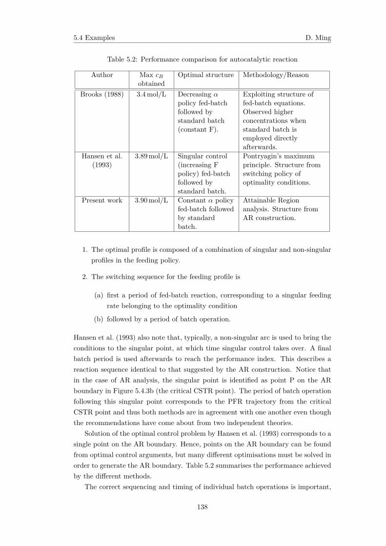
5.4 Examples D. Ming
Table 5.2: Performance comparison for autocatalytic reaction
Author Max cBobtained
Optimal structure Methodology/Reason
Brooks (1988) 3.4mol/L Decreasing αpolicy fed-batchfollowed bystandard batch(constant F).
Exploiting structure offed-batch equations.Observed higherconcentrations whenstandard batch isemployed directlyafterwards.
Hansen et al.(1993)
3.89mol/L Singular control(increasing Fpolicy) fed-batchfollowed bystandard batch.
Pontryagin’s maximumprinciple. Structure fromswitching policy ofoptimality conditions.
Present work 3.90mol/L Constant α policyfed-batch followedby standardbatch.
Attainable Regionanalysis. Structure fromAR construction.
1. The optimal profile is composed of a combination of singular and non-singularprofiles in the feeding policy.
2. The switching sequence for the feeding profile is
(a) first a period of fed-batch reaction, corresponding to a singular feedingrate belonging to the optimality condition
(b) followed by a period of batch operation.
Hansen et al. (1993) also note that, typically, a non-singular arc is used to bring theconditions to the singular point, at which time singular control takes over. A finalbatch period is used afterwards to reach the performance index. This describes areaction sequence identical to that suggested by the AR construction. Notice thatin the case of AR analysis, the singular point is identified as point P on the ARboundary in Figure 5.4.3b (the critical CSTR point). The period of batch operationfollowing this singular point corresponds to the PFR trajectory from the criticalCSTR point and thus both methods are in agreement with one another even thoughthe recommendations have come about from two independent theories.
Solution of the optimal control problem by Hansen et al. (1993) corresponds to asingle point on the AR boundary. Hence, points on the AR boundary can be foundfrom optimal control arguments, but many different optimisations must be solved inorder to generate the AR boundary. Table 5.2 summarises the performance achievedby the different methods.
The correct sequencing and timing of individual batch operations is important,
138
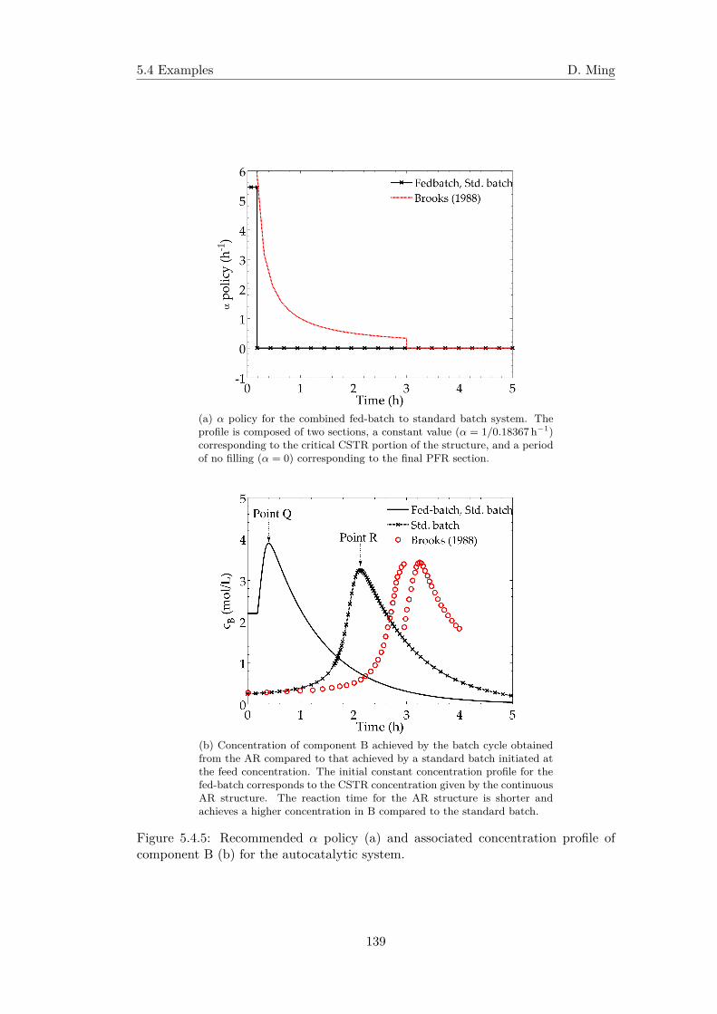
5.4 Examples D. Ming
(a) α policy for the combined fed-batch to standard batch system. Theprofile is composed of two sections, a constant value (α = 1/0.18367h−1)corresponding to the critical CSTR portion of the structure, and a periodof no filling (α = 0) corresponding to the final PFR section.
(b) Concentration of component B achieved by the batch cycle obtainedfrom the AR compared to that achieved by a standard batch initiated atthe feed concentration. The initial constant concentration profile for thefed-batch corresponds to the CSTR concentration given by the continuousAR structure. The reaction time for the AR structure is shorter andachieves a higher concentration in B compared to the standard batch.
Figure 5.4.5: Recommended α policy (a) and associated concentration profile ofcomponent B (b) for the autocatalytic system.
139
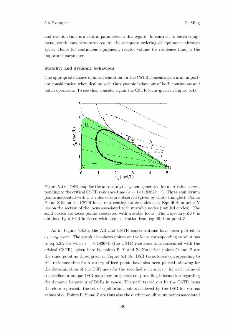
5.4 Examples D. Ming
and reaction time is a central parameter in this regard. In contrast to batch equip-ment, continuous structures require the adequate ordering of equipment throughspace. Hence for continuous equipment, reactor volume (or residence time) is theimportant parameter.
Stability and dynamic behaviour
The appropriate choice of initial condition for the CSTR concentration is an import-ant consideration when dealing with the dynamic behaviour of both continuous andbatch operation. To see this, consider again the CSTR locus given in Figure 5.4.6.
Figure 5.4.6: DSR map for the autocatalytic system generated for an α value corres-ponding to the critical CSTR residence time (α = 1/0.18367h−1). Three equilibriumpoints associated with this value of α are observed (given by white triangles). PointsP and Z lie on the CSTR locus representing stable nodes (×). Equilibrium point Ylies on the section of the locus associated with unstable nodes (unfilled circles). Thesolid circles are locus points associated with a stable focus. The trajectory ZUV isobtained by a PFR initiated with a concentration from equilibrium point Z.
As in Figure 5.4.3b, the AR and CSTR concentrations have been plotted incA − cB space. The graph also shows points on the locus corresponding to solutionsto eq 5.2.2 for when τ = 0.18367h (the CSTR residence time associated with thecritical CSTR), given here by points P, Y and Z. Note that points O and P arethe same point as those given in Figure 5.4.3b. DSR trajectories corresponding tothis residence time for a variety of feed points have also been plotted, allowing forthe determination of the DSR map for the specified α in space – for each value ofα specified, a unique DSR map may be generated, providing information regardingthe dynamic behaviour of DSRs in space. The path traced out by the CSTR locustherefore represents the set of equilibrium points achieved by the DSR for variousvalues of α. Points P, Y and Z are thus also the distinct equilibrium points associated
140
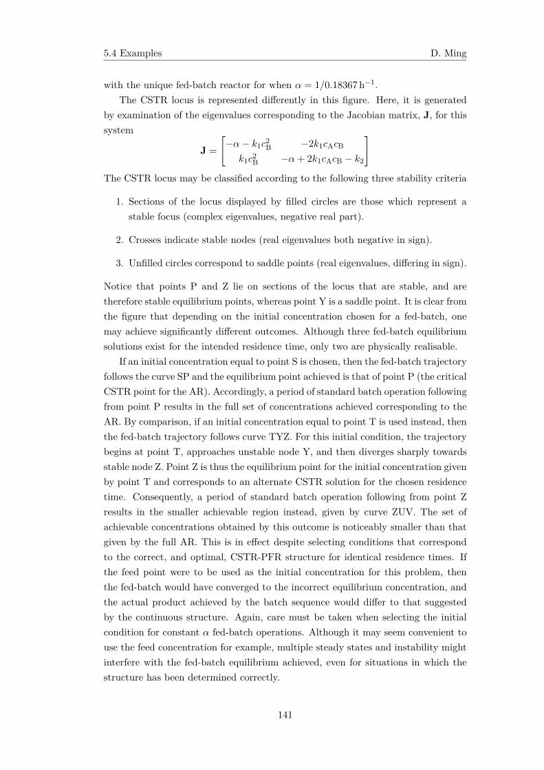
5.4 Examples D. Ming
with the unique fed-batch reactor for when α = 1/0.18367h−1.The CSTR locus is represented differently in this figure. Here, it is generated
by examination of the eigenvalues corresponding to the Jacobian matrix, J, for thissystem
J =
[−α− k1c
2B −2k1cAcB
k1c2B −α+ 2k1cAcB − k2
]The CSTR locus may be classified according to the following three stability criteria
1. Sections of the locus displayed by filled circles are those which represent astable focus (complex eigenvalues, negative real part).
2. Crosses indicate stable nodes (real eigenvalues both negative in sign).
3. Unfilled circles correspond to saddle points (real eigenvalues, differing in sign).
Notice that points P and Z lie on sections of the locus that are stable, and aretherefore stable equilibrium points, whereas point Y is a saddle point. It is clear fromthe figure that depending on the initial concentration chosen for a fed-batch, onemay achieve significantly different outcomes. Although three fed-batch equilibriumsolutions exist for the intended residence time, only two are physically realisable.
If an initial concentration equal to point S is chosen, then the fed-batch trajectoryfollows the curve SP and the equilibrium point achieved is that of point P (the criticalCSTR point for the AR). Accordingly, a period of standard batch operation followingfrom point P results in the full set of concentrations achieved corresponding to theAR. By comparison, if an initial concentration equal to point T is used instead, thenthe fed-batch trajectory follows curve TYZ. For this initial condition, the trajectorybegins at point T, approaches unstable node Y, and then diverges sharply towardsstable node Z. Point Z is thus the equilibrium point for the initial concentration givenby point T and corresponds to an alternate CSTR solution for the chosen residencetime. Consequently, a period of standard batch operation following from point Zresults in the smaller achievable region instead, given by curve ZUV. The set ofachievable concentrations obtained by this outcome is noticeably smaller than thatgiven by the full AR. This is in effect despite selecting conditions that correspondto the correct, and optimal, CSTR-PFR structure for identical residence times. Ifthe feed point were to be used as the initial concentration for this problem, thenthe fed-batch would have converged to the incorrect equilibrium concentration, andthe actual product achieved by the batch sequence would differ to that suggestedby the continuous structure. Again, care must be taken when selecting the initialcondition for constant α fed-batch operations. Although it may seem convenient touse the feed concentration for example, multiple steady states and instability mightinterfere with the fed-batch equilibrium achieved, even for situations in which thestructure has been determined correctly.
141
5.4 Examples D. Ming
5.4.2 3D van de Vusse kinetics
System specification
Next, we shall examine the nature of the optimal batch structure for the well-knownvan de Vusse reaction scheme. Consideration of this system will demonstrate therole that DSRs, and by extension, the role that fed-batch reactors with varying α
policies play in the formation the AR boundary. The system is composed of threeindependent reactions, that is,
A k1→ B k2→ C
2A →k3
D
Although four species are present, only three are independent, as the fourth may bedetermined by mass balance. The rate expression follows mass-action kinetics andmay be written in terms of components A and B by the following rate vector
r (C) =
−k1cA − 2k3c2A
k1cA − k2cB
k3c2A
The associated rate constants are then given as k1 = 1h−1, k2 = 1h−1, k3 =
10L/ (mol · h). Historically, the associated AR has been determined in cA − cB − cD
space, so that the concentration vector may be expressed as C = [cA, cB, cD]T. We
specify that the feed is pure in component A, in which case Cf = [1, 0, 0]T.Construction of the AR for the above problem has been discussed in previous
work, and the optimal structure is well understood (Hildebrandt and Glasser, 1990;Feinberg and Hildebrandt, 1997). As a result, we are able to utilise the previouslydeveloped results and apply them here with very little added effort, so that thedevelopment of an equivalent batch structure may be carried out. A brief summaryof the construction procedure for the system is provided below for completeness.
Optimal continuous structure
Only the feed point is achievable initially. As with many AR construction problems,it is most natural to begin by considering single reactor structures that expand theinitial set of achievable points from the feed. The simplest method of achieving thisis by computing the PFR trajectory and CSTR locus from Cf. This is equivalent tothe procedure performed for the 2D van de Vusse system in chapter 5.
PFRs and CSTR locus from the feed PFRs make up the final approach tothe extremities of the AR boundary and thus it is helpful to include PFR segmentsas the final reactor to all structures. In effect, we wish to generate the convex
142
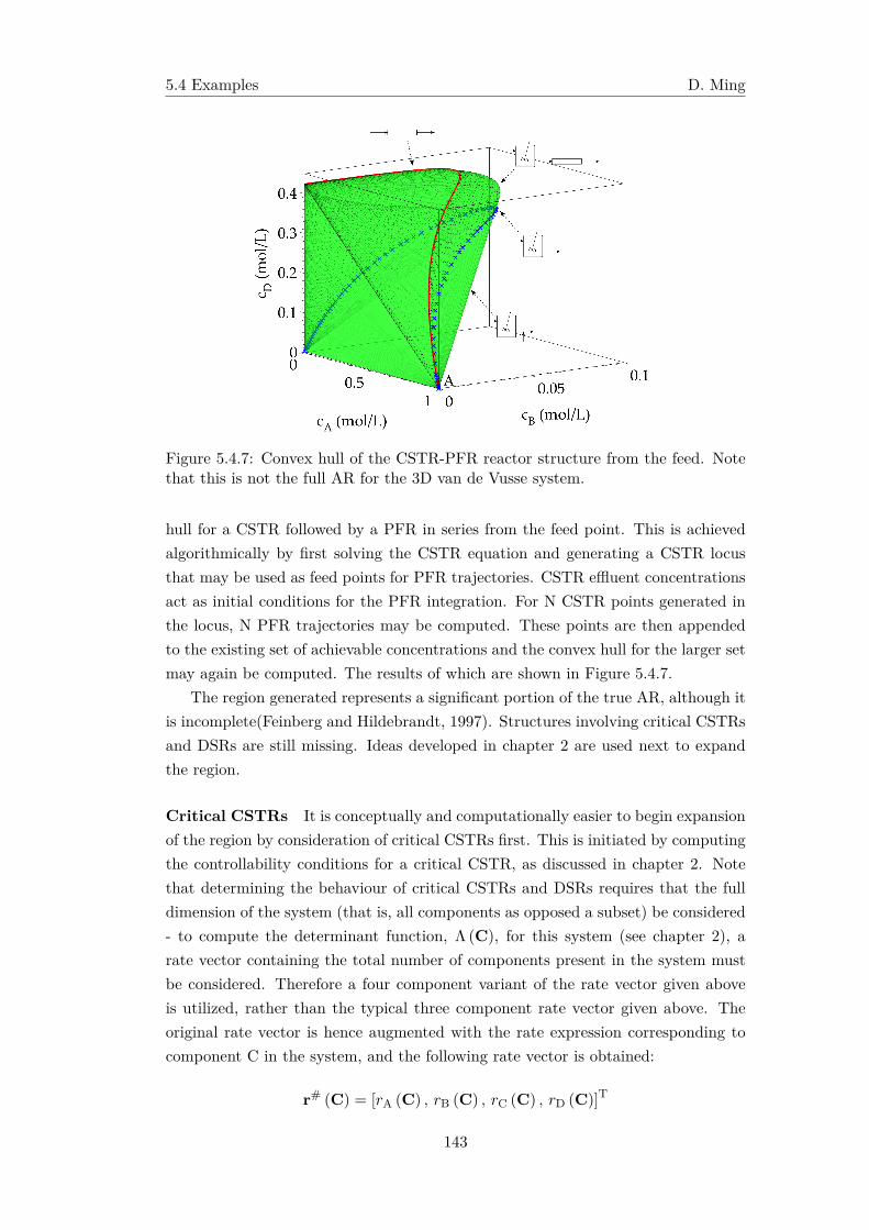
5.4 Examples D. Ming
Figure 5.4.7: Convex hull of the CSTR-PFR reactor structure from the feed. Notethat this is not the full AR for the 3D van de Vusse system.
hull for a CSTR followed by a PFR in series from the feed point. This is achievedalgorithmically by first solving the CSTR equation and generating a CSTR locusthat may be used as feed points for PFR trajectories. CSTR effluent concentrationsact as initial conditions for the PFR integration. For N CSTR points generated inthe locus, N PFR trajectories may be computed. These points are then appendedto the existing set of achievable concentrations and the convex hull for the larger setmay again be computed. The results of which are shown in Figure 5.4.7.
The region generated represents a significant portion of the true AR, although itis incomplete(Feinberg and Hildebrandt, 1997). Structures involving critical CSTRsand DSRs are still missing. Ideas developed in chapter 2 are used next to expandthe region.
Critical CSTRs It is conceptually and computationally easier to begin expansionof the region by consideration of critical CSTRs first. This is initiated by computingthe controllability conditions for a critical CSTR, as discussed in chapter 2. Notethat determining the behaviour of critical CSTRs and DSRs requires that the fulldimension of the system (that is, all components as opposed a subset) be considered- to compute the determinant function, Λ (C), for this system (see chapter 2), arate vector containing the total number of components present in the system mustbe considered. Therefore a four component variant of the rate vector given aboveis utilized, rather than the typical three component rate vector given above. Theoriginal rate vector is hence augmented with the rate expression corresponding tocomponent C in the system, and the following rate vector is obtained:
r# (C) = [rA (C) , rB (C) , rC (C) , rD (C)]T
143
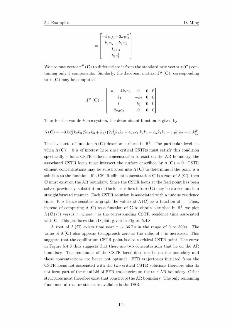
5.4 Examples D. Ming
=
−k1cA − 2k3c
2A
k1cA − k2cB
k2cB
k3c2A
We use rate vector r# (C) to differentiate it from the standard rate vector r (C) con-taining only 3 components. Similarly, the Jacobian matrix, J# (C), correspondingto r′ (C) may be computed
J# (C) =
−k1 − 4k3cA 0 0 0
k1 −k2 0 0
0 k2 0 0
2k3cA 0 0 0
Thus for the van de Vusse system, the determinant function is given by:
Λ (C) = −3.5c3Ak2k3 (2cAk3 + k1)(2c2Ak1k3 − 4cAcBk2k3 − cAk1k2 − cBk1k2 + cBk
22
)The level sets of function Λ (C) describe surfaces in R3. The particular level setwhen Λ (C) = 0 is of interest here since critical CSTRs must satisfy this conditionspecifically – for a CSTR effluent concentration to exist on the AR boundary, theassociated CSTR locus must intersect the surface described by Λ (C) = 0. CSTReffluent concentrations may be substituted into Λ (C) to determine if the point is asolution to the function. If a CSTR effluent concentration C is a root of Λ (C), thenC must exist on the AR boundary. Since the CSTR locus at the feed point has beensolved previously, substitution of the locus values into Λ (C) may be carried out in astraightforward manner. Each CSTR solution is associated with a unique residencetime. It is hence sensible to graph the values of Λ (C) as a function of τ . Thus,instead of computing Λ (C) as a function of C to obtain a surface in R3, we plotΛ (C (τ)) versus τ , where τ is the corresponding CSTR residence time associatedwith C. This produces the 2D plot, given in Figure 5.4.8.
A root of Λ (C) exists time near τ ∼ 36.7 s in the range of 0 to 300 s. Thevalue of Λ (C) also appears to approach zero as the value of τ is increased. Thissuggests that the equilibrium CSTR point is also a critical CSTR point. The curvein Figure 5.4.8 thus suggests that there are two concentrations that lie on the ARboundary. The remainder of the CSTR locus does not lie on the boundary andthese concentrations are hence not optimal. PFR trajectories initiated from theCSTR locus not associated with the two critical CSTR solutions therefore also donot form part of the manifold of PFR trajectories on the true AR boundary. Otherstructures must therefore exist that constitute the AR boundary. The only remainingfundamental reactor structure available is the DSR.
144
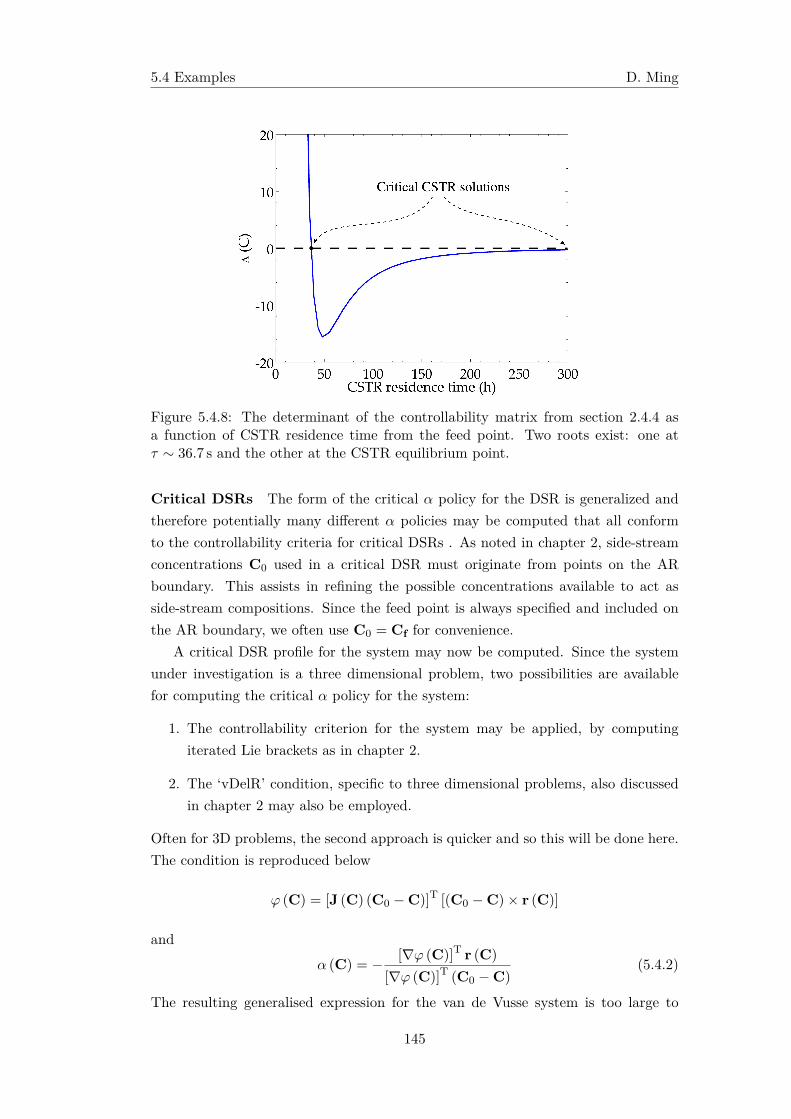
5.4 Examples D. Ming
Figure 5.4.8: The determinant of the controllability matrix from section 2.4.4 asa function of CSTR residence time from the feed point. Two roots exist: one atτ ∼ 36.7 s and the other at the CSTR equilibrium point.
Critical DSRs The form of the critical α policy for the DSR is generalized andtherefore potentially many different α policies may be computed that all conformto the controllability criteria for critical DSRs . As noted in chapter 2, side-streamconcentrations C0 used in a critical DSR must originate from points on the ARboundary. This assists in refining the possible concentrations available to act asside-stream compositions. Since the feed point is always specified and included onthe AR boundary, we often use C0 = Cf for convenience.
A critical DSR profile for the system may now be computed. Since the systemunder investigation is a three dimensional problem, two possibilities are availablefor computing the critical α policy for the system:
1. The controllability criterion for the system may be applied, by computingiterated Lie brackets as in chapter 2.
2. The ‘vDelR’ condition, specific to three dimensional problems, also discussedin chapter 2 may also be employed.
Often for 3D problems, the second approach is quicker and so this will be done here.The condition is reproduced below
φ (C) = [J (C) (C0 − C)]T [(C0 − C)× r (C)]
andα (C) = − [∇φ (C)]T r (C)
[∇φ (C)]T (C0 − C)(5.4.2)
The resulting generalised expression for the van de Vusse system is too large to
145
5.4 Examples D. Ming
display in terms of all system variables alone. Numerical values for the kinetic con-stants and mixing point may be substituted into eq 5.4.2 to simplify the expressionslightly. The expression given in Feinberg (2000b) is then obtained.
α (C) =1
2
[cA
(20cA
3cB − 80cA2cB − cA
2 + 37cAcB + cA + 2cB)
cB (cA2 − 2cA + 1)
](5.4.3)
Note that eq 5.4.3 is specific to the feed point C0 = Cf = [1, 0, 0]T and the valuesof the rate constants given at the beginning of the example. If different conditionsare used, eq 5.4.2 must again be employed and simplified for the new α expression.
Initial conditions for the DSR are next considered. It is intuitive to initiate aDSR from the feed point. The DSR expression is thus integrated together with thecritical � policy provided previously to produce a DSR trajectory. We note that eq5.4.3 is undefined at C = C0. Hence, to initiate the integration, the initial conditionfor the DSR is offset slightly from feed point value. Hence, an initial condition ofCf = [0.9999, 0.0001, 0]T is supplied as opposed to [1, 0, 0]T. The DSR equationis then integrated together with eq 5.4.3 over a sufficiently long integration time.The resulting profile is given in Figure 5.4.9a. The convex hull corresponding to thiscandidate is not shown here so that the underlying boundary structures are moreeasily identified.
This produces a critical DSR trajectory in space. Note that although the DSRtrajectory appears to behave in a similar fashion to the CSTR locus, the sets ofconcentrations produced by the two are distinct. All of the points on the criticalDSR trajectory lie on the AR boundary. PFR trajectories in series with the DSRwill therefore serve to fill out a manifold of extreme points on the AR boundary.These trajectories are also displayed in the figure.
It is interesting to note that the critical DSR trajectory obtained in Figure 5.4.9aterminates at an intermediate point near CSTR locus. This is labelled as point B inFigure 5.4.9a. The second critical CSTR solution located at the equilibrium pointdoes not appear to intersect the DSR trajectory. Since the AR boundary is composedof PFR trajectories connected by critical CSTRs and DSRs, a portion of the ARboundary is missing that joins the two critical CSTR points obtained previouslytogether. Additional DSR structures must exist that connect the two critical pointstogether that are not currently associated with the proposed structure.
To identify the other critical DSR, a bit of deduction is necessary: Since thefeed point Cf has already been utilized as an initial condition to the critical DSRthat passes through one of two critical CSTR points (the DSR equilibrium con-centration is at the critical CSTR concentration), the only critical concentrationavailable is that of the other critical CSTR point obtained at the CSTR equilibriumconcentration.
Accordingly, to complete construction of the AR boundary, another DSR tra-
146
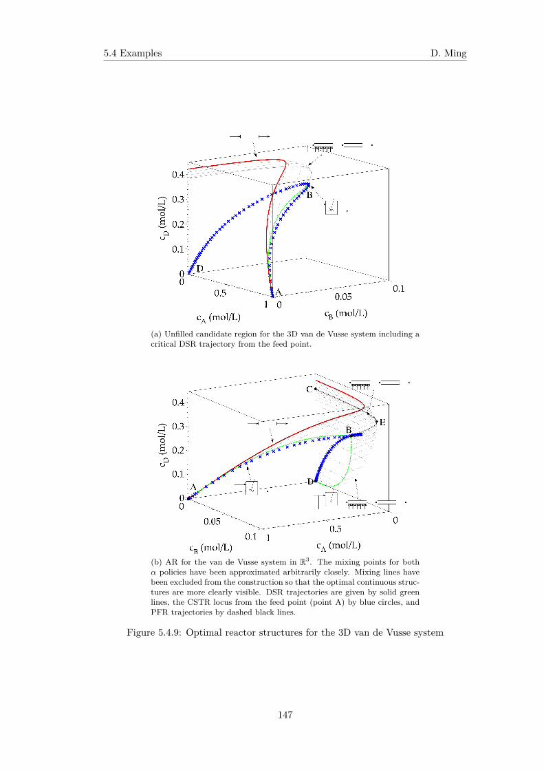
5.4 Examples D. Ming
(a) Unfilled candidate region for the 3D van de Vusse system including acritical DSR trajectory from the feed point.
(b) AR for the van de Vusse system in R3. The mixing points for bothα policies have been approximated arbitrarily closely. Mixing lines havebeen excluded from the construction so that the optimal continuous struc-tures are more clearly visible. DSR trajectories are given by solid greenlines, the CSTR locus from the feed point (point A) by blue circles, andPFR trajectories by dashed black lines.
Figure 5.4.9: Optimal reactor structures for the 3D van de Vusse system
147
5.4 Examples D. Ming
jectory is initiated at the CSTR equilibrium point. When this is performed, theresulting critical DSR trajectory is different to that initiated at Cf: the trajectoryappears to connect the two critical CSTR concentrations together. This second DSRtrajectory is a further connector on the AR boundary. PFR trajectories are againinitiated from critical DSR trajectory to fill out the remaining bottom portion of theAR boundary. This is serves to complete construction of the AR boundary for the3D van de Vusse system. All reactor structures forming the AR boundary is givenin Figure 5.4.9b.
A summary of the optimal structures is thus given as follows:
1. Structure 1: A DSR from the feed vector (point A) to equilibrium (point B)followed by a PFR to equilibrium (point C). This fills out the first part of theAR boundary (path ABEC).
2. Structure 2: A CSTR operating at its equilibrium (point D), followed by aDSR at equilibrium (point B) and then a PFR. The unique PFR trajectoryBEC that passes through point E is the point of maximum concentration incomponent B. This fills out the underside of the AR boundary (path DBEC).
The kinetics exhibit three independent reactions and hence, at most, two parallelreaction schemes are required to achieve all concentrations on the AR boundary.Combination of these two reactor structures alone allows for the synthesis of everypossible concentration for every possible reactor configuration imaginable. A dis-tinct choice must be made between the two depending upon the desired final state.Different optimizations may now be carried out to identify points where the ARboundary and objective function intersect. Once these intersection points have beenestablished, the appropriate optimal reactor structures may be employed to achievethe points of interest. Notice that the above structures are consistent with what itexpected from the theory discussed in chapter 2:
• The AR is convex.
• DSR trajectories and CSTR critical points form connectors to a manifold ofPFR extreme points.
• The boundary of the AR is composed of straight line sections (indicating mix-ing) and PFR trajectories only. The final approach to all reactive portions ofthe boundary is achieved via a PFR.
This concludes the AR construction for the 3D van de Vusse kinetics. Notice thatthe inclusion of critical CSTRs and DSRs complicates construction, but these arerequired in order to generate the true AR.
148
5.4 Examples D. Ming
Conversion to batch
For this example, the AR is defined by two parallel continuous structures. It followsthat we require, at most, two batch structures to achieve all points on the ARboundary. Figure 5.4.10 provides the necessary conversion from continuous to batch.Again, a one-to-one correspondence between batch and continuous equipment isobserved. In both cases, fed-batch reactors with varying α policies are seen tocontribute significantly to the overall set of achievable concentrations.
The following batch cycles are required (Figure 5.4.10b):
• For structure 1, a fed-batch reactor followed by a period of standard batchreaction. This is provided by path ABEC in Figure 5.4.9b.
• For structure 2, three distinct reaction intervals are needed, two of whichare fed-batch operations. The cycle is initiated with a period of constant α,followed by a non-constant α interval, and completed with a period of standardbatch reaction. This is given in Figure 5.4.9b by the path DBEC.
Again, as these structures are analogous to the original continuous equipment, bothmay be used to achieve point E. Unless one is interested in achieving concentrationsalong the unique PFR trajectory BC, reduced segments belonging to structures 1 and2 such as those of AFG and DHI can be used. For concentrations occurring withinthe region however, combinations of these structures along with mixing betweenthem may be used.
Effect of different objective functions
Now that the AR and its associated batch structures have been determined, optim-isation for a number of scenarios may be investigated. Suppose that it is desiredto achieve the maximum amount of intermediate component B. By the above dis-cussion, both structures in Figure 5.4.10 pass through point E and therefore bothmay be used to achieve maximum B. Suppose, instead, that we wish to limit theformation of component D to a maximum value of 0.3mol/L whilst still achievingmaximum B. This point must lie on the intersection of the AR boundary and theplane described by cD = 0.3mol/L; this is obtainable by structure 2 (given hereby Figure 5.4.11). By comparison, assume that it is decided to find the maximumamount of B for cD = 0.4mol/L instead. We find that structure 1 is now required,and thus the nature of the batch cycle is different. Both of these scenarios how-ever, are contained within the structure of the AR. The AR is composed of at mosttwo unique structures, and as a result, all concentrations on the boundary may
149
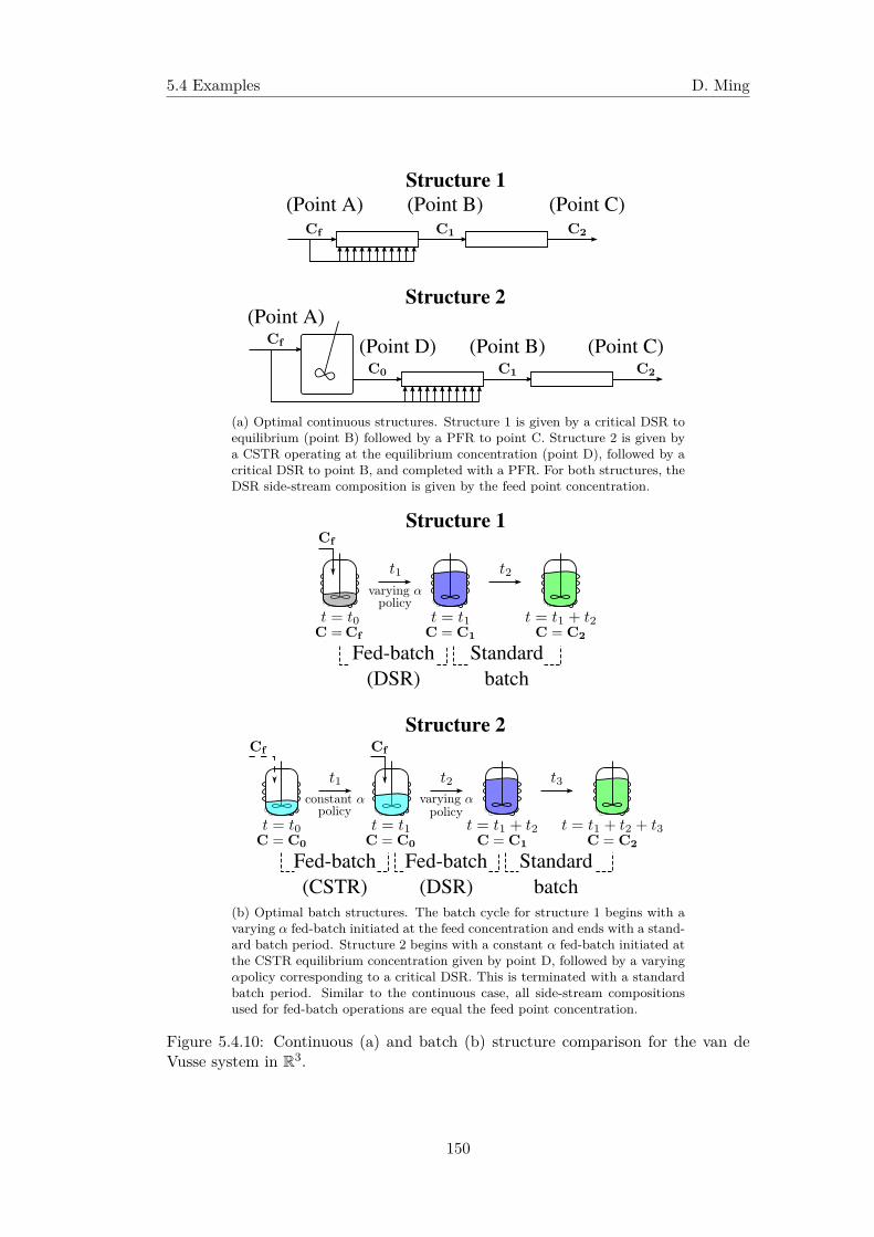
5.4 Examples D. Ming
Structure 2
Structure 1(Point A) (Point B) (Point C)
(Point A)(Point D) (Point B) (Point C)
(a) Optimal continuous structures. Structure 1 is given by a critical DSR toequilibrium (point B) followed by a PFR to point C. Structure 2 is given bya CSTR operating at the equilibrium concentration (point D), followed by acritical DSR to point B, and completed with a PFR. For both structures, theDSR side-stream composition is given by the feed point concentration.
Structure 2
Structure 1
Fed-batch(CSTR)
Fed-batch(DSR)
Standard batch
Fed-batch(DSR)
Standard batch
(b) Optimal batch structures. The batch cycle for structure 1 begins with avarying α fed-batch initiated at the feed concentration and ends with a stand-ard batch period. Structure 2 begins with a constant α fed-batch initiated atthe CSTR equilibrium concentration given by point D, followed by a varyingαpolicy corresponding to a critical DSR. This is terminated with a standardbatch period. Similar to the continuous case, all side-stream compositionsused for fed-batch operations are equal the feed point concentration.
Figure 5.4.10: Continuous (a) and batch (b) structure comparison for the van deVusse system in R3.
150
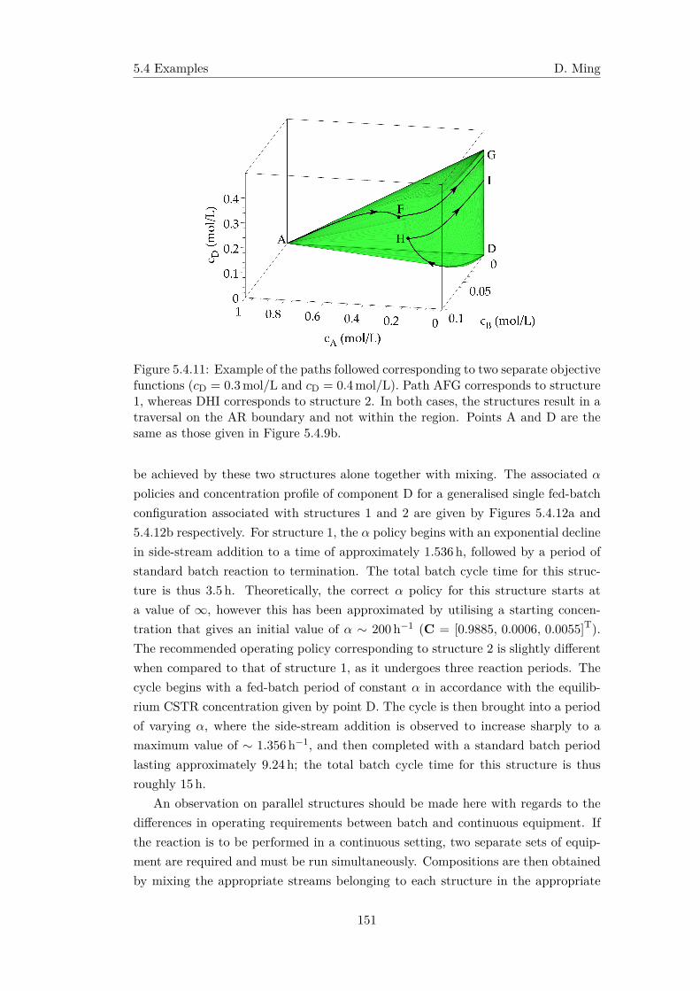
5.4 Examples D. Ming
Figure 5.4.11: Example of the paths followed corresponding to two separate objectivefunctions (cD = 0.3mol/L and cD = 0.4mol/L). Path AFG corresponds to structure1, whereas DHI corresponds to structure 2. In both cases, the structures result in atraversal on the AR boundary and not within the region. Points A and D are thesame as those given in Figure 5.4.9b.
be achieved by these two structures alone together with mixing. The associated α
policies and concentration profile of component D for a generalised single fed-batchconfiguration associated with structures 1 and 2 are given by Figures 5.4.12a and5.4.12b respectively. For structure 1, the α policy begins with an exponential declinein side-stream addition to a time of approximately 1.536h, followed by a period ofstandard batch reaction to termination. The total batch cycle time for this struc-ture is thus 3.5h. Theoretically, the correct α policy for this structure starts ata value of ∞, however this has been approximated by utilising a starting concen-tration that gives an initial value of α ∼ 200h−1 (C = [0.9885, 0.0006, 0.0055]T).The recommended operating policy corresponding to structure 2 is slightly differentwhen compared to that of structure 1, as it undergoes three reaction periods. Thecycle begins with a fed-batch period of constant α in accordance with the equilib-rium CSTR concentration given by point D. The cycle is then brought into a periodof varying α, where the side-stream addition is observed to increase sharply to amaximum value of ∼ 1.356h−1, and then completed with a standard batch periodlasting approximately 9.24 h; the total batch cycle time for this structure is thusroughly 15h.
An observation on parallel structures should be made here with regards to thedifferences in operating requirements between batch and continuous equipment. Ifthe reaction is to be performed in a continuous setting, two separate sets of equip-ment are required and must be run simultaneously. Compositions are then obtainedby mixing the appropriate streams belonging to each structure in the appropriate
151
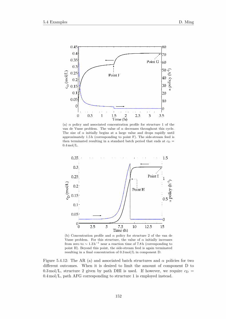
5.4 Examples D. Ming
(a) α policy and associated concentration profile for structure 1 of thevan de Vusse problem. The value of α decreases throughout this cycle.The size of α initially begins at a large value and drops rapidly untilapproximately 1.5h (corresponding to point F). The side-stream feed isthen terminated resulting in a standard batch period that ends at cD =0.4mol/L.
(b) Concentration profile and α policy for structure 2 of the van deVusse problem. For this structure, the value of α initially increasesfrom zero to ∼ 1.3h−1 near a reaction time of 7.8 h (corresponding topoint H). Beyond this point, the side-stream feed is again terminatedresulting in a final concentration of 0.3mol/L in component D.
Figure 5.4.12: The AR (a) and associated batch structures and α policies for twodifferent outcomes. When it is desired to limit the amount of component D to0.3mol/L, structure 2 given by path DHI is used. If however, we require cD =0.4mol/L, path AFG corresponding to structure 1 is employed instead.
152
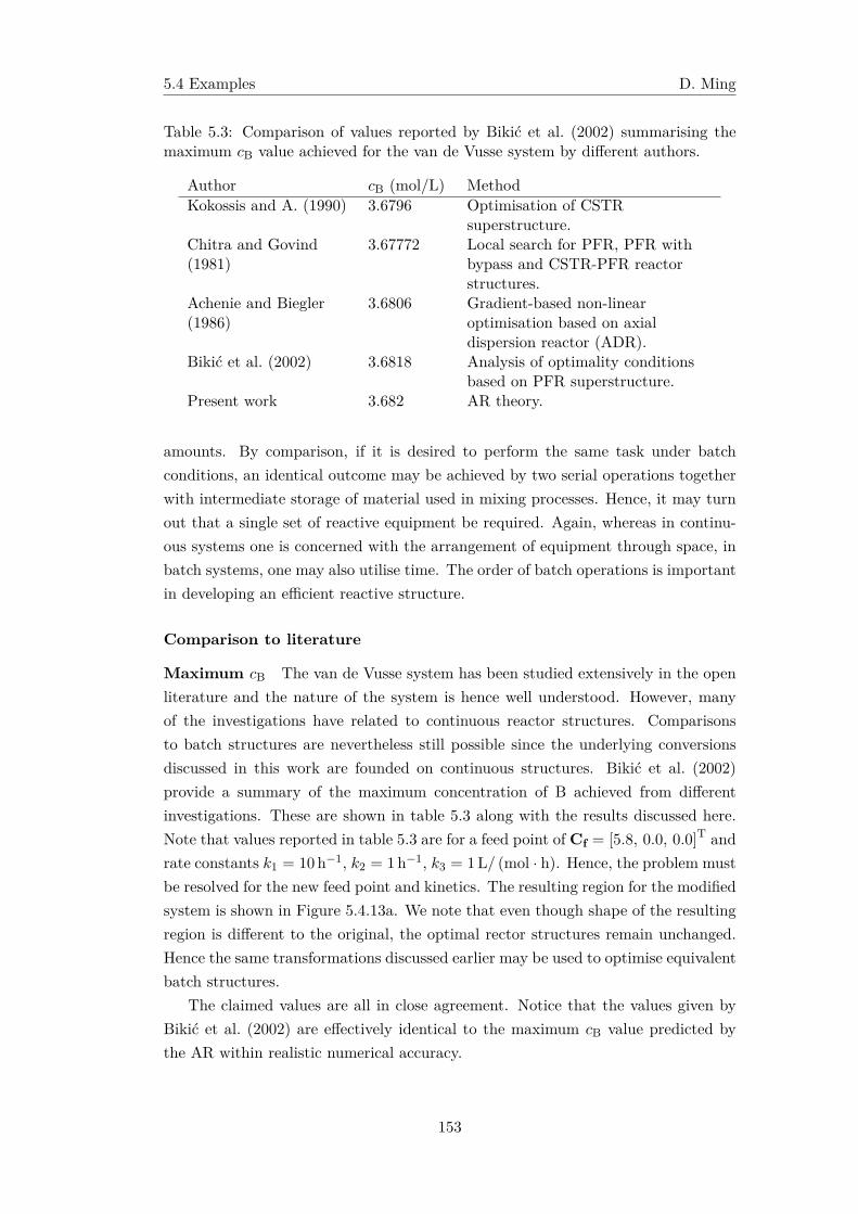
5.4 Examples D. Ming
Table 5.3: Comparison of values reported by Bikić et al. (2002) summarising themaximum cB value achieved for the van de Vusse system by different authors.
Author cB (mol/L) MethodKokossis and A. (1990) 3.6796 Optimisation of CSTR
superstructure.Chitra and Govind(1981)
3.67772 Local search for PFR, PFR withbypass and CSTR-PFR reactorstructures.
Achenie and Biegler(1986)
3.6806 Gradient-based non-linearoptimisation based on axialdispersion reactor (ADR).
Bikić et al. (2002) 3.6818 Analysis of optimality conditionsbased on PFR superstructure.
Present work 3.682 AR theory.
amounts. By comparison, if it is desired to perform the same task under batchconditions, an identical outcome may be achieved by two serial operations togetherwith intermediate storage of material used in mixing processes. Hence, it may turnout that a single set of reactive equipment be required. Again, whereas in continu-ous systems one is concerned with the arrangement of equipment through space, inbatch systems, one may also utilise time. The order of batch operations is importantin developing an efficient reactive structure.
Comparison to literature
Maximum cB The van de Vusse system has been studied extensively in the openliterature and the nature of the system is hence well understood. However, manyof the investigations have related to continuous reactor structures. Comparisonsto batch structures are nevertheless still possible since the underlying conversionsdiscussed in this work are founded on continuous structures. Bikić et al. (2002)provide a summary of the maximum concentration of B achieved from differentinvestigations. These are shown in table 5.3 along with the results discussed here.Note that values reported in table 5.3 are for a feed point of Cf = [5.8, 0.0, 0.0]T andrate constants k1 = 10 h−1, k2 = 1h−1, k3 = 1L/ (mol · h). Hence, the problem mustbe resolved for the new feed point and kinetics. The resulting region for the modifiedsystem is shown in Figure 5.4.13a. We note that even though shape of the resultingregion is different to the original, the optimal rector structures remain unchanged.Hence the same transformations discussed earlier may be used to optimise equivalentbatch structures.
The claimed values are all in close agreement. Notice that the values given byBikić et al. (2002) are effectively identical to the maximum cB value predicted bythe AR within realistic numerical accuracy.
153
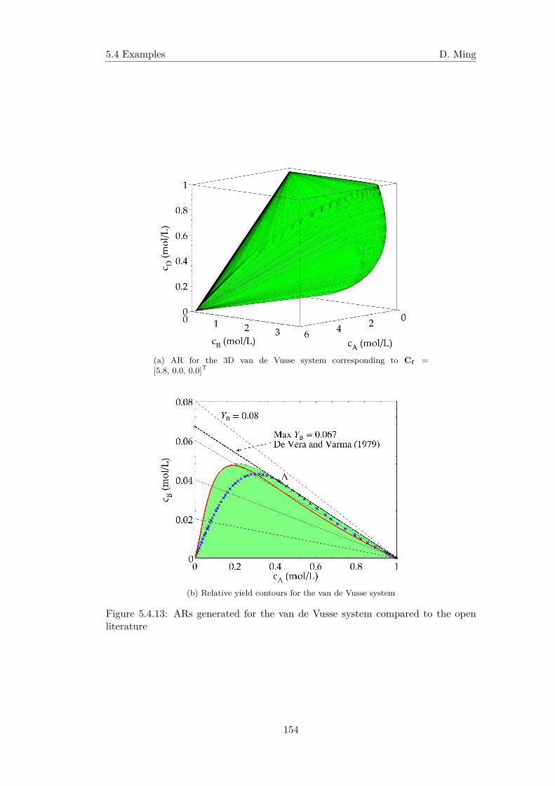
5.4 Examples D. Ming
(a) AR for the 3D van de Vusse system corresponding to Cf =[5.8, 0.0, 0.0]T
(b) Relative yield contours for the van de Vusse system
Figure 5.4.13: ARs generated for the van de Vusse system compared to the openliterature
154
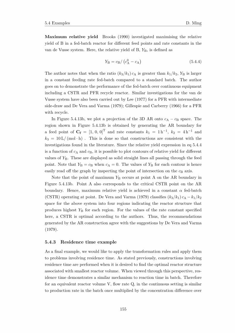
5.4 Examples D. Ming
Maximum relative yield Brooks (1990) investigated maximising the relativeyield of B in a fed-batch reactor for different feed points and rate constants in thevan de Vusse system. Here, the relative yield of B, YB, is defined as
YB = cB/(c0A − cA
)(5.4.4)
The author notes that when the ratio (k3/k1) cA is greater than k1/k2, YB is largerin a constant feeding rate fed-batch compared to a standard batch. The authorgoes on to demonstrate the performance of the fed-batch over continuous equipmentincluding a CSTR and PFR recycle reactor. Similar investigations for the van deVusse system have also been carried out by Lee (1977) for a PFR with intermediateside-draw and De Vera and Varma (1979); Gillespie and Carberry (1966) for a PFRwith recycle.
In Figure 5.4.13b, we plot a projection of the 3D AR onto cA − cB space. Theregion shown in Figure 5.4.13b is obtained by generating the AR boundary fora feed point of Cf = [1, 0, 0]T and rate constants k1 = 1 h−1, k2 = 4 h−1 andk3 = 10L/ (mol · h) . This is done so that constructions are consistent with theinvestigations found in the literature. Since the relative yield expression in eq 5.4.4is a function of cA and cB, it is possible to plot contours of relative yield for differentvalues of YB. These are displayed as solid straight lines all passing through the feedpoint. Note that YB = cB when cA = 0. The values of YB for each contour is henceeasily read off the graph by inspecting the point of intersection on the cB axis.
Note that the point of maximum YB occurs at point A on the AR boundary inFigure 5.4.13b. Point A also corresponds to the critical CSTR point on the ARboundary. Hence, maximum relative yield is achieved in a constant α fed-batch(CSTR) operating at point. De Vera and Varma (1979) classifies (k3/k1) cA − k1/k2
space for the above system into four regions indicating the reactor structure thatproduces highest YB for each region. For the values of the rate constant specifiedhere, a CSTR is optimal according to the authors. Thus, the recommendationsgenerated by the AR construction agree with the suggestions by De Vera and Varma(1979).
5.4.3 Residence time example
As a final example, we would like to apply the transformation rules and apply themto problems involving residence time. As stated previously, constructions involvingresidence time are performed when it is desired to find the optimal reactor structureassociated with smallest reactor volume. When viewed through this perspective, res-idence time demonstrates a similar mechanism to reaction time in batch. Thereforefor an equivalent reactor volume V, flow rate Q, in the continuous setting is similarto production rate in the batch once multiplied by the concentration difference over
155
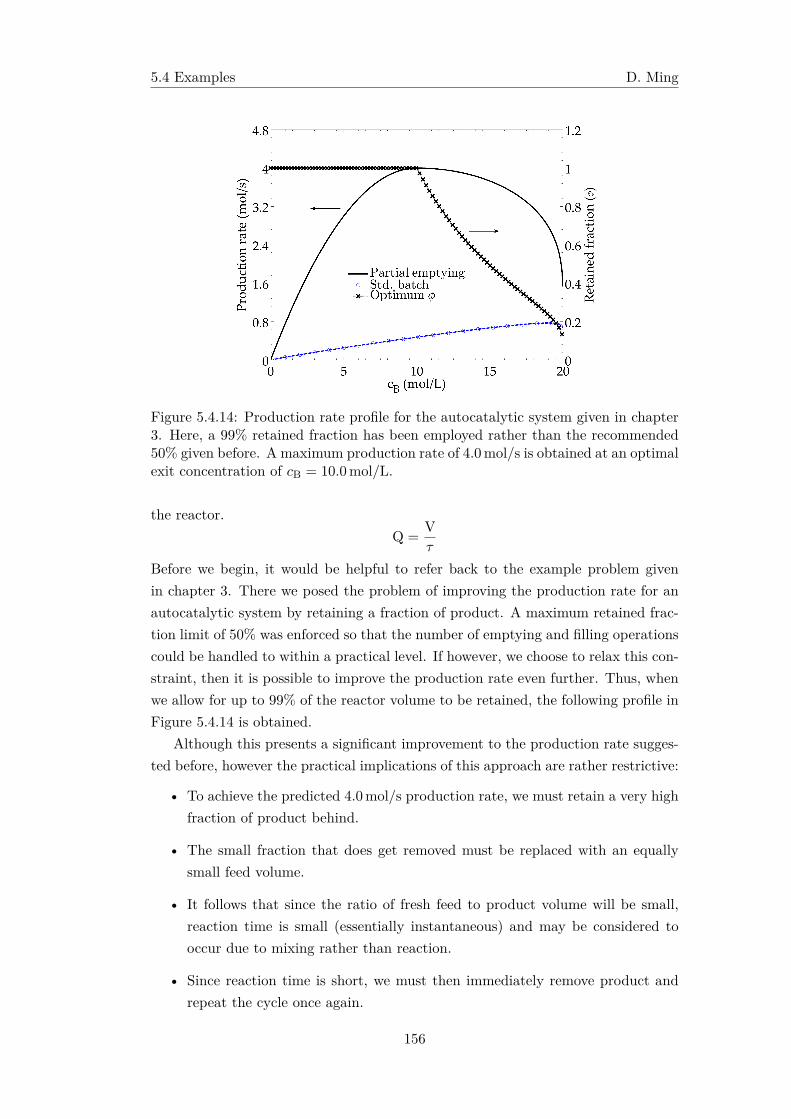
5.4 Examples D. Ming
Figure 5.4.14: Production rate profile for the autocatalytic system given in chapter3. Here, a 99% retained fraction has been employed rather than the recommended50% given before. A maximum production rate of 4.0mol/s is obtained at an optimalexit concentration of cB = 10.0mol/L.
the reactor.Q =
Vτ
Before we begin, it would be helpful to refer back to the example problem givenin chapter 3. There we posed the problem of improving the production rate for anautocatalytic system by retaining a fraction of product. A maximum retained frac-tion limit of 50% was enforced so that the number of emptying and filling operationscould be handled to within a practical level. If however, we choose to relax this con-straint, then it is possible to improve the production rate even further. Thus, whenwe allow for up to 99% of the reactor volume to be retained, the following profile inFigure 5.4.14 is obtained.
Although this presents a significant improvement to the production rate sugges-ted before, however the practical implications of this approach are rather restrictive:
• To achieve the predicted 4.0mol/s production rate, we must retain a very highfraction of product behind.
• The small fraction that does get removed must be replaced with an equallysmall feed volume.
• It follows that since the ratio of fresh feed to product volume will be small,reaction time is small (essentially instantaneous) and may be considered tooccur due to mixing rather than reaction.
• Since reaction time is short, we must then immediately remove product andrepeat the cycle once again.
156
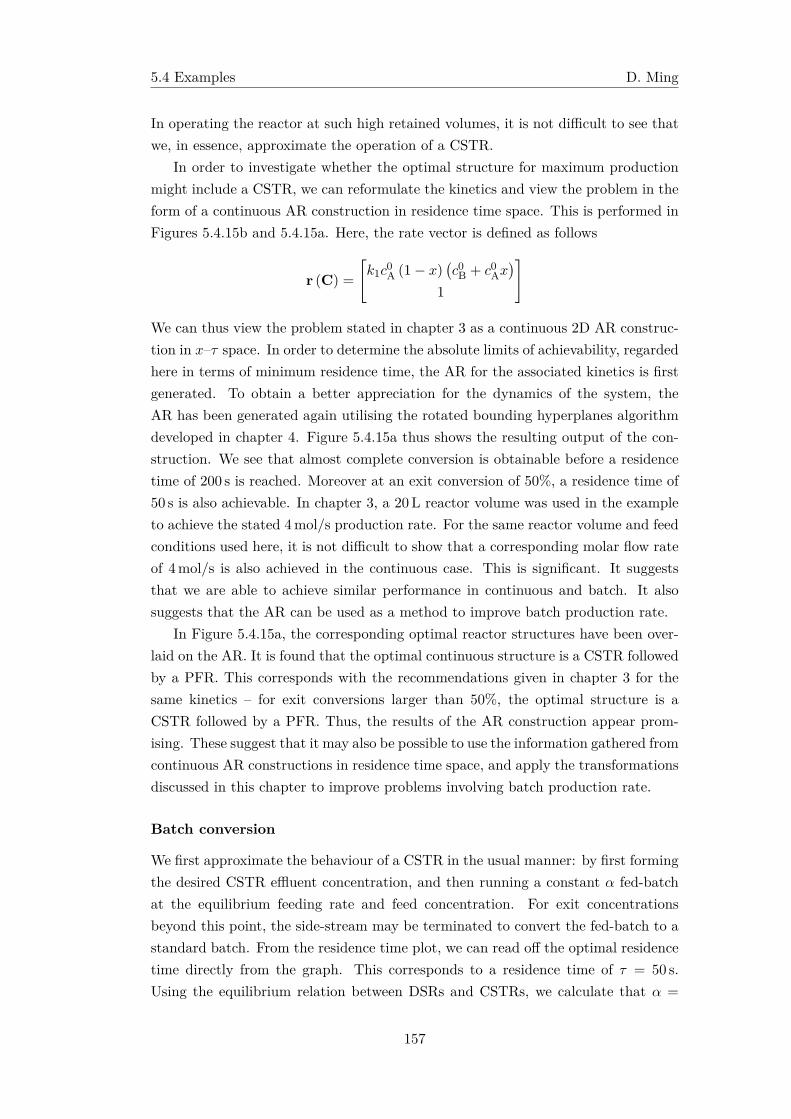
5.4 Examples D. Ming
In operating the reactor at such high retained volumes, it is not difficult to see thatwe, in essence, approximate the operation of a CSTR.
In order to investigate whether the optimal structure for maximum productionmight include a CSTR, we can reformulate the kinetics and view the problem in theform of a continuous AR construction in residence time space. This is performed inFigures 5.4.15b and 5.4.15a. Here, the rate vector is defined as follows
r (C) =
[k1c
0A (1− x)
(c0B + c0Ax
)1
]
We can thus view the problem stated in chapter 3 as a continuous 2D AR construc-tion in x–τ space. In order to determine the absolute limits of achievability, regardedhere in terms of minimum residence time, the AR for the associated kinetics is firstgenerated. To obtain a better appreciation for the dynamics of the system, theAR has been generated again utilising the rotated bounding hyperplanes algorithmdeveloped in chapter 4. Figure 5.4.15a thus shows the resulting output of the con-struction. We see that almost complete conversion is obtainable before a residencetime of 200 s is reached. Moreover at an exit conversion of 50%, a residence time of50 s is also achievable. In chapter 3, a 20L reactor volume was used in the exampleto achieve the stated 4mol/s production rate. For the same reactor volume and feedconditions used here, it is not difficult to show that a corresponding molar flow rateof 4mol/s is also achieved in the continuous case. This is significant. It suggeststhat we are able to achieve similar performance in continuous and batch. It alsosuggests that the AR can be used as a method to improve batch production rate.
In Figure 5.4.15a, the corresponding optimal reactor structures have been over-laid on the AR. It is found that the optimal continuous structure is a CSTR followedby a PFR. This corresponds with the recommendations given in chapter 3 for thesame kinetics – for exit conversions larger than 50%, the optimal structure is aCSTR followed by a PFR. Thus, the results of the AR construction appear prom-ising. These suggest that it may also be possible to use the information gathered fromcontinuous AR constructions in residence time space, and apply the transformationsdiscussed in this chapter to improve problems involving batch production rate.
Batch conversion
We first approximate the behaviour of a CSTR in the usual manner: by first formingthe desired CSTR effluent concentration, and then running a constant α fed-batchat the equilibrium feeding rate and feed concentration. For exit concentrationsbeyond this point, the side-stream may be terminated to convert the fed-batch to astandard batch. From the residence time plot, we can read off the optimal residencetime directly from the graph. This corresponds to a residence time of τ = 50 s.Using the equilibrium relation between DSRs and CSTRs, we calculate that α =
157
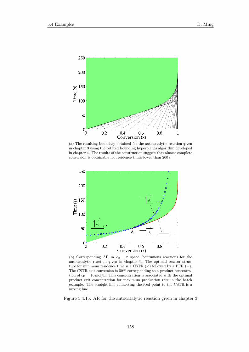
5.4 Examples D. Ming
(a) The resulting boundary obtained for the autocatalytic reaction givenin chapter 3 using the rotated bounding hyperplanes algorithm developedin chapter 4. The results of the construction suggest that almost completeconversion is obtainable for residence times lower than 200 s.
(b) Corresponding AR in cB − τ space (continuous reaction) for theautocatalytic reaction given in chapter 3. The optimal reactor struc-ture for minimum residence time is a CSTR (×) followed by a PFR (−).The CSTR exit conversion is 50% corresponding to a product concentra-tion of cB = 10mol/L. This concentration is associated with the optimalproduct exit concentration for maximum production rate in the batchexample. The straight line connecting the feed point to the CSTR is amixing line.
Figure 5.4.15: AR for the autocatalytic reaction given in chapter 3
158
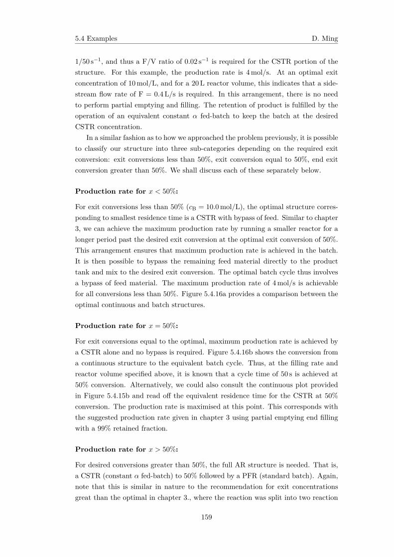
5.4 Examples D. Ming
1/50 s−1, and thus a F/V ratio of 0.02 s−1 is required for the CSTR portion of thestructure. For this example, the production rate is 4mol/s. At an optimal exitconcentration of 10mol/L, and for a 20L reactor volume, this indicates that a side-stream flow rate of F = 0.4L/s is required. In this arrangement, there is no needto perform partial emptying and filling. The retention of product is fulfilled by theoperation of an equivalent constant α fed-batch to keep the batch at the desiredCSTR concentration.
In a similar fashion as to how we approached the problem previously, it is possibleto classify our structure into three sub-categories depending on the required exitconversion: exit conversions less than 50%, exit conversion equal to 50%, end exitconversion greater than 50%. We shall discuss each of these separately below.
Production rate for x < 50%:
For exit conversions less than 50% (cB = 10.0mol/L), the optimal structure corres-ponding to smallest residence time is a CSTR with bypass of feed. Similar to chapter3, we can achieve the maximum production rate by running a smaller reactor for alonger period past the desired exit conversion at the optimal exit conversion of 50%.This arrangement ensures that maximum production rate is achieved in the batch.It is then possible to bypass the remaining feed material directly to the producttank and mix to the desired exit conversion. The optimal batch cycle thus involvesa bypass of feed material. The maximum production rate of 4mol/s is achievablefor all conversions less than 50%. Figure 5.4.16a provides a comparison between theoptimal continuous and batch structures.
Production rate for x = 50%:
For exit conversions equal to the optimal, maximum production rate is achieved bya CSTR alone and no bypass is required. Figure 5.4.16b shows the conversion froma continuous structure to the equivalent batch cycle. Thus, at the filling rate andreactor volume specified above, it is known that a cycle time of 50 s is achieved at50% conversion. Alternatively, we could also consult the continuous plot providedin Figure 5.4.15b and read off the equivalent residence time for the CSTR at 50%conversion. The production rate is maximised at this point. This corresponds withthe suggested production rate given in chapter 3 using partial emptying end fillingwith a 99% retained fraction.
Production rate for x > 50%:
For desired conversions greater than 50%, the full AR structure is needed. That is,a CSTR (constant α fed-batch) to 50% followed by a PFR (standard batch). Again,note that this is similar in nature to the recommendation for exit concentrationsgreat than the optimal in chapter 3., where the reaction was split into two reaction
159
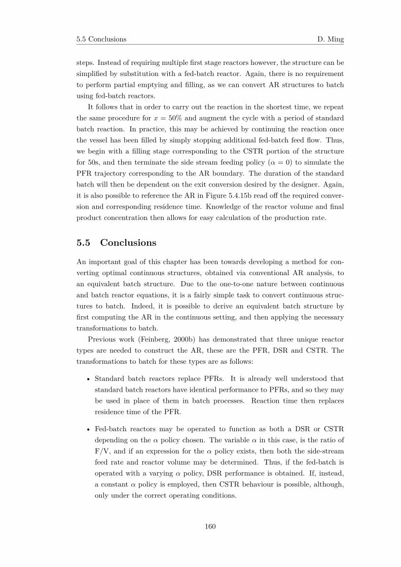
5.5 Conclusions D. Ming
steps. Instead of requiring multiple first stage reactors however, the structure can besimplified by substitution with a fed-batch reactor. Again, there is no requirementto perform partial emptying and filling, as we can convert AR structures to batchusing fed-batch reactors.
It follows that in order to carry out the reaction in the shortest time, we repeatthe same procedure for x = 50% and augment the cycle with a period of standardbatch reaction. In practice, this may be achieved by continuing the reaction oncethe vessel has been filled by simply stopping additional fed-batch feed flow. Thus,we begin with a filling stage corresponding to the CSTR portion of the structurefor 50s, and then terminate the side stream feeding policy (α = 0) to simulate thePFR trajectory corresponding to the AR boundary. The duration of the standardbatch will then be dependent on the exit conversion desired by the designer. Again,it is also possible to reference the AR in Figure 5.4.15b read off the required conver-sion and corresponding residence time. Knowledge of the reactor volume and finalproduct concentration then allows for easy calculation of the production rate.
5.5 Conclusions
An important goal of this chapter has been towards developing a method for con-verting optimal continuous structures, obtained via conventional AR analysis, toan equivalent batch structure. Due to the one-to-one nature between continuousand batch reactor equations, it is a fairly simple task to convert continuous struc-tures to batch. Indeed, it is possible to derive an equivalent batch structure byfirst computing the AR in the continuous setting, and then applying the necessarytransformations to batch.
Previous work (Feinberg, 2000b) has demonstrated that three unique reactortypes are needed to construct the AR, these are the PFR, DSR and CSTR. Thetransformations to batch for these types are as follows:
• Standard batch reactors replace PFRs. It is already well understood thatstandard batch reactors have identical performance to PFRs, and so they maybe used in place of them in batch processes. Reaction time then replacesresidence time of the PFR.
• Fed-batch reactors may be operated to function as both a DSR or CSTRdepending on the α policy chosen. The variable α in this case, is the ratio ofF/V, and if an expression for the α policy exists, then both the side-streamfeed rate and reactor volume may be determined. Thus, if the fed-batch isoperated with a varying α policy, DSR performance is obtained. If, instead,a constant α policy is employed, then CSTR behaviour is possible, although,only under the correct operating conditions.
160
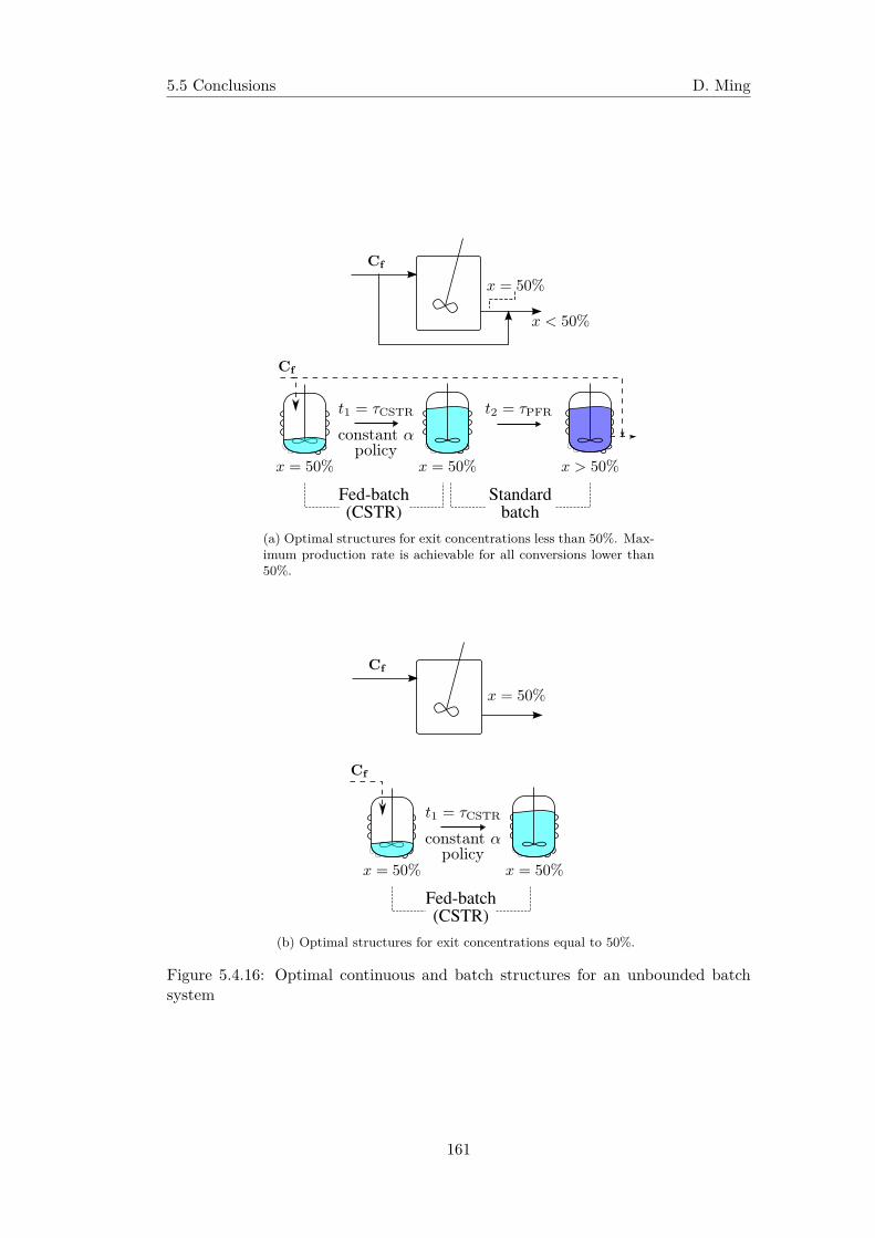
5.5 Conclusions D. Ming
Fed-batch(CSTR)
Standard batch
(a) Optimal structures for exit concentrations less than 50%. Max-imum production rate is achievable for all conversions lower than50%.
Fed-batch(CSTR)
(b) Optimal structures for exit concentrations equal to 50%.
Figure 5.4.16: Optimal continuous and batch structures for an unbounded batchsystem
161
5.5 Conclusions D. Ming
Fed-batch(CSTR)
Standard batch
(c) Optimal structures for exit concentrations greater than 50%.In this instance, maximum production rate is not achieved, thoughthis arrangement is still the optimal for smallest residence time andhence optimal for best production rate.
Figure 5.4.16: Optimal continuous and batch structures for an unbounded batchsystem
For each value of α, there exists an associated equilibrium concentration that mustbe used. Possibly many equilibrium points may be obtained for kinetics involvingmultiple steady states. This is related to the equivalence found between CSTRsand constant α DSRs operating at equilibrium. Constant α fed-batch reactors thusmimic CSTRs at the equilibrium point. This results in interesting operational con-sequences:
1. Fed-batch reactors must be initiated and operated at a concentration equalto that of the equivalent CSTR effluent composition. The concentration ofspecies within the fed-batch is constant during this period of reaction as aresult. Reaction time is also determined by the filling rate and vessel volume.
2. Various methods may be used to achieve the initial CSTR composition, al-though these methods may be ineffective in obtaining the desired CSTR com-position if the corresponding DSR equilibrium point is unstable. In practice,if the desired CSTR point unstable, one may wish to introduce a stabilisingcontroller to realise the desired state.
Thus, care must be taken when choosing an initial concentration for the fed-batchfor converting structures containing CSTRs to an equivalent batch. It is generallynot sufficient to choose an initial concentration in an arbitrary manner in the hopeto reach a desired CSTR concentration. The dynamic behaviour of the system,in the form of multiple steady states and instability, may not allow one to do so.Furthermore, it might not be possible to achieve the desired CSTR concentration
162
5.5 Conclusions D. Ming
if the associated equilibrium point corresponding to eq 5.3.3 proves to be unstable. At the time of writing, we have yet to encounter systems in which the desiredequilibrium point belonging to a critical CSTR is also unstable, however the pos-sibility should not be overlooked. Such a situation could prove to be troublesomefor both continuous and batch structures, as both the CSTR and fed-batch may notbe controllable without further work to stabilise the state. Otherwise, one wouldthen need to work within a constrained region of the full AR utilising points thatare known to be stable.
We also investigated the use of ARs constructed in residence time space as ameans of improving the production rate in a batch reactor. It was observed thatresidence time provides a similar metric to batch reaction time. Thus, there existsa relation between the reactor volume and flow rate in a continuous setting, to anequivalent volume and production rate in a batch. However, although it is possibleto mix residence time, it is not possible to achieve the same in the batch equivalent.This investigation was performed on the same worked example provided in chapter3. We noticed that unlike the recommendations given in chapter 3, we do not needto employ a partial emptying and filling strategy to achieve maximum performance.Instead, the approach used here is to relate the optimal reactor structure associ-ated with smallest residence time to an equivalent batch operating policy using thetransformations provided in this chapter. In place of a partial emptying and fillingstage followed by a standard batch, we employ a constant α fed-batch followed bya standard batch. The production rate achieved by this approach corresponds tothe same volumetric flow rate in the continuous case, and so the method is consist-ent. It follows that AR constructions involving more than one independent reactionmight also be used to improve a batch with the same kinetics and feed composition,however this has not been tested in this work.
Although the work given in chapter 3 appears to be subsumed by that givenhere, we note that the two methods apply to different design scenarios: The formermay be employed in the absence of a kinetic model, when only experimental dataare available, whereas the the latter relies on AR theory, which in turn relies onspecification of a well defined rate field and feed point in order to generate the AR.It is difficult to generate a candidate region using only the results of chapter 3, evenif these ideas are founded on principles in AR theory. Nevertheless, if kinetics issupplied, with the intention of improving batch production rates, then the ideaspresented here are more easily generalised for many independent reactions.
Finally, although many similarities between batch equipment in time and con-tinuous equipment in space exist, a number of differences are also noted.
1. It may be possible to achieve all concentrations belonging to the AR by asingle reaction vessel in batch systems, whereas for continuous equipment, aphysically separate set of reactors is required for each branch of the recom-
163
References D. Ming
mended AR structure. By the same reasoning, one should also be mindful ofthe order that batch operations are carried out, as different batch operatingpolicies may be required for different points desired in or on the AR boundary.
2. If a single batch reactor is employed, one may be constrained if bypass mixingwith a stream downstream concentration at a future time is employed. Con-tinuous equipment for a spatial reactor network are superior in this regard.This may also be overcome in a batch if intermediate storage is utilised formixing with subsequent reaction stages in future cycles.
3. From general AR theory it is known that DSRs are not required for continuoussystems involving two independent reactions. The familiar VdelR condition ofchapter 2 is a consequence of this. However, since CSTRs are approximatedin a batch environment by use of constant α fed-batch rectors, which are ana-logous to DSRs in the continuous setting, DSRs are generally still requiredin batch unless the optimal reactor structure for the associated 2D system isa convex PFR. Note that these fed-batch trajectories do not fulfill the samefunction as critical DSR trajectories, but rather they approximate CSTR con-centrations. Besides critical CSTR points, these fed-batch trajectories operateinside the AR. Hence, if a particular optimisation scenario is employed inwhich the objective function intersects the CSTR locus at a point other thanthe critical CSTR point, then this may be awkward to realise with fed-batchreactors.
The above discussion suggests that improvement in batch reactors is possible bya geometric approach. Interpretation of the problem first as a continuous systemallows for the determination of the AR, which provides insight into the limits ofachievability for all reactor structures. This, in turn, guides the choice of reactorstructure employed. Consideration of the AR thus offers a different method of po-tential improvement in batch reactors. The AR and its corresponding structurestherefore serve the dual purpose of establishing a set of recommended reactor con-figurations that may be used to improve both batch and continuous equipment froma single configuration.
References
Abraham, T. K., Feinberg, M., 2004. Kinetic bounds on attainability in the reactorsynthesis problem. Industrial & Engineering Chemistry Research 43 (2), 449–457.
Achenie, L. E., Biegler, L. T., 1986. Algorithmic synthesis of chemical reactor net-works using mathematical programming. Industrial and Engineering ChemistryFundamentals 25 (4), 621–627.
Allgor, R. J., Barrera, M. D., Barton, P. I., Evans, L. B., 1996. Optimal batchprocess development. Computers & Chemical Engineering 20 (6-7), 885–896.
164
References D. Ming
Allgor, R. J., Barton, P. I., 9 1999. Screening models for batch process development:Part ii. case studies. Chemical Engineering Science 54 (18), 4065–4087.
Allgor, R. J., Evans, L. B., Barton, P. I., 10 1999. Screening models for batch processdevelopment: Part i. design targets for reaction/distillation networks. ChemicalEngineering Science 54 (19), 4145–4164.
Aziz, N., Mujtaba, I. M., 1 2002. Optimal operation policies in batch reactors.Chemical Engineering Journal 85 (2-3), 313–325.
Balakotaiah, V., Luss, D., 1982. Exact steady-state multiplicity criteria for two con-secutive or parallel reactions in lumped-parameter systems. Chemical EngineeringScience 37 (3), 433–445.
Balakotaiah, V., Luss, D., 1983. Multiplicity features of reacting systems: depend-ence of the steady-states of a cstr on the residence time. Chemical EngineeringScience 38 (10), 1709–1721.
Balakotaiah, V., Luss, D., 1984. Global analysis of the multiplicity features ofmulti-reaction lumped-parameter systems. Chemical Engineering Science 39 (5),865–881.
Bikić, D., Butinar, B., Glavič, P., 2002. Optimal reactor systems for van de vussereaction scheme with multicomponent feed. Computers & Chemical Engineering26 (10), 1335–1343.
Bonvin, D., 1998. Optimal operation of batch reactors - a personal view. Journal ofProcess Control 8 (5-6), 355–368.
Brooks, B. W., 1988. Semi-batch reactors and their use for autocatalytic reactions.Chemical Engineering Science 43 (6), 1287–1290.
Brooks, B. W., 1990. Product yields from the van de vusse reaction scheme: use ofsemi-batch reactors. Chemical Engineering Science 45 (6), 1589–1594.
Burri, J. F., Wilson, S. D., Manousiouthakis, V. I., 2002. Infinite dimensional state-space approach to reactor network synthesis: Application to attainable regionconstruction. Computers & Chemical Engineering 26 (6), 849–862.
Capon-Garcia, E., Bojarski, A. D., Espuna, A., Puigjaner, L., 2011. Multiobjectiveoptimization of multiproduct batch plants scheduling under environmental andeconomic concerns. AIChE Journal 57 (10), 2766–2782.
Cheong, D.-Y., Hansen, C. L., Stevens, D. K., 2007. Production of bio-hydrogenby mesophilic anaerobic fermentation in an acid-phase sequencing batch reactor.Biotechnology and bioengineering 96 (3), 421–432.
Chitra, S. P., Govind, R., 1981. Yield optimization for complex reactor systems.Chemical Engineering Science 36 (7), 1219–1225.
Davies, W. L., Gloor, W. T., 1971. Batch production of pharmaceutical granulationsin a fluidized bed i: Effects of process variables on physical properties of finalgranulation. Journal of pharmaceutical sciences 60 (12), 1869–1874.
Davis, B. J., Taylor, L. A., Manousiouthakis, V. I., 2008. Identification of the at-
165
References D. Ming
tainable region for batch reactor networks. Industrial & Engineering ChemistryResearch 47 (10), 3388–3400.
De Vera, A. L., Varma, A., 1979. Yield optimization for the van de vusse reaction.The Chemical Engineering Journal 17 (2), 163–167.
Feinberg, M., 1999. Recent results in optimal reactor synthesis via attainable regiontheory. Chemical Engineering Science 54 (13-14), 2535–2543.
Feinberg, M., 2000a. Optimal reactor design from a geometric viewpoint - iii. criticalcfstrs. Chemical Engineering Science 55 (17), 3553–3565.
Feinberg, M., 2000b. Optimal reactor design from a geometric viewpoint. part ii.critical sidestream reactors. Chemical Engineering Science 55 (13), 2455–2479.
Feinberg, M., Hildebrandt, D., 1997. Optimal reactor design from a geometricviewpoint- i. universal properties of the attainable region. Chemical EngineeringScience 52 (10), 1637–1665.
Gillespie, B., Carberry, J., 1966. Reactor yield at intermediate mixing levels–anextension of van de vusse’s analysis. Chemical Engineering Science 21 (5), 472–475.
Glasser, D., Hildebrandt, D., 1997. Reactor and process synthesis. Computers &Chemical Engineering 21 (Supplement 1), S775–S783.
Glasser, D., Hildebrandt, D., Crowe, C., 1987. A geometric approach to steady flowreactors: The attainable region and optimization in concentration space. Industrial& Engineering Chemistry Research 26 (9), 1803–1810.
Godorr, S., Hildebrandt, D., Glasser, D., McGregor, C., 1999. Choosing optimalcontrol policies using the attainable region approach. Industrial & EngineeringChemistry Research 38 (3), 639–651.
Godorr, S. A., Hildebrandt, D., Glasser, D., 1994. The attainable region for systemswith mixing and multiple-rate processes: finding optimal reactor structures. TheChemical Engineering Journal and The Biochemical Engineering Journal 54 (3),175–186.
Gray, P., Scott, S. K., 1983. Autocatalytic reactions in the isothermal, continuousstirred tank reactor : Isolas and other forms of multistability. Chemical Engineer-ing Science 38 (1), 29–43.
Gray, P., Scott, S. K., 1984. Autocatalytic reactions in the isothermal, continuousstirred tank reactor : Oscillations and instabilities in the system a + 2b -> 3b; b-> c. Chemical Engineering Science 39 (6), 1087–1097.
Hansen, J. M., Lim, H. C., Hong, J., 1993. Optimization of autocatalytic reactions.Chemical Engineering Science 48 (13), 2375–2390.
Hildebrandt, D., Glasser, D., 1990. The attainable region and optimal reactor struc-tures. Chemical Engineering Science 45 (8), 2161–2168.
Hildebrandt, D., Glasser, D., Crowe, C. M., 1990. Geometry of the attainable regiongenerated by reaction and mixing: With and without constraints. Industrial &Engineering Chemistry Research 29 (1), 49–58.
166
References D. Ming
Kauchali, S., Rooney, W. C., Biegler, L. T., Glasser, D., Hildebrandt, D., 2002.Linear programming formulations for attainable region analysis. Chemical Engin-eering Science 57 (11), 2015–2028.
Khumalo, N., Glasser, D., Hildebrandt, D., Hausberger, B., Kauchali, S., 2006. Theapplication of the attainable region analysis to comminution. Chemical Engineer-ing Science 61 (18), 5969–5980.
Kokossis, A. C., A., F. C., 1990. Optimization of complex reactor networks - i.isothermal operation. Chemical Engineering Science 45 (3), 595–614.
Kondepudi, D. K., Asakura, K., 2001. Chiral autocatalysis, spontaneous symmetrybreaking, and stochastic behavior. Accounts of chemical research 34 (12), 946–954.
Lee, H. H., 1977. Tubular reactor with recycle from an intermediate point: yield ofvan de vusse’s reactions. Chemical Engineering Science 32 (5), 562–563.
Maestri, F., Rota, R., 2007. Safe and productive operation of homogeneoussemibatch reactors involving autocatalytic reactions with arbitrary reaction or-der. Industrial & Engineering Chemistry Research 46 (16), 5333–5339.
Manousiouthakis, V. I., Justanieah, A. M., Taylor, L. A., 2004. The shrink-wrapalgorithm for the construction of the attainable region: An application of theideas framework. Computers & Chemical Engineering 28 (9), 1563–1575.
Mendez, C. A., Cerda, J., Grossmann, I. E., Harjunkoski, I., Fahl, M., 2006. State-of-the-art review of optimization methods for short-term scheduling of batch pro-cesses. Computers & Chemical Engineering 30 (6-7), 913–946.
Ming, D., Hildebrandt, D., Glasser, D., 2010. A revised method of attainable re-gion construction utilizing rotated bounding hyperplanes. Industrial & Engineer-ing Chemistry Research 49 (21), 10549–10557.
Modak, J. M., Lim, H. C., 1992. Optimal mode of operation of bioreactor for fer-mentation processes. Chemical Engineering Science 47 (15-16), 3869–3884.
Najafpour, G., Younesi, H., Ismail, K. S. K., 2004. Ethanol fermentation in animmobilized cell reactor using saccharomyces cerevisiae. Bioresource technology92 (3), 251–260.
Nicol, W., Hernier, M., Hildebrant, D., Glasser, D., 2001. The attainable region andprocess synthesis: Reaction systems with external cooling and heating. the effectof relative cost of reactor volume to heat exchange area on the optimal processlayout. Chemical Engineering Science 56 (1), 173–191.
Nicol, W., Hildebrandt, D., Glasser, D., 1997. Process synthesis for reaction systemswith cooling via finding the attainable region. Computers & Chemical Engineering21 (Supplement 1), S35–S40.
Nisoli, A., Malone, M. F., Doherty, M. F., 1997. Attainable regions for reaction withseparation. AIChE Journal 43 (2), 374–386.
Putot, A., Gallice, F., Hoff, C., Guillot, V., 2002. Thermal stability of an oligosac-charide: Autocatalytic behavior. Organic process research & development 6 (6),901–905.
167
References D. Ming
Rooney, W. C., Hausberger, B. P., Biegler, L. T., Glasser, D., 2000. Convex at-tainable region projections for reactor network synthesis. Computers & ChemicalEngineering 24 (2-7), 225–229.
Schlosser, P. M., Feinberg, M., 1994. A theory of multiple steady states in isothermalhomogeneous cfstrs with many reactions. Chemical Engineering Science 49 (11),1749–1767.
Senthuran, A., Senthuran, V., Mattiasson, B., Kaul, R., 1997. Lactic acid fermenta-tion in a recycle batch reactor using immobilized lactobacillus casei. Biotechnologyand bioengineering 55 (6), 841–853.
Seodigeng, T., Hausberger, B., Hildebrandt, D., Glasser, D., 2009. Recursive con-stant control policy algorithm for attainable regions analysis. Computers & Chem-ical Engineering 33 (1), 309–320.
Strogatz, S. H., 2001. Nonlinear Dynamics And Chaos: With Applications To Phys-ics, Biology, Chemistry, And Engineering. Westview Press, Ch. 5.
Subotic, B., 1989. Influence of autocatalytic nucleation on zeolite crystallizationprocesses. In: ACS symposium series. Vol. 398. pp. 110–123.
Watzky, M. A., Morris, A. M., Ross, E. D., Finke, R. G., 2008. Fitting yeast andmammalian prion aggregation kinetic data with the finke- watzky two-step modelof nucleation and autocatalytic growth. Biochemistry 47 (40), 10790–10800.
Woolard, C. R., Irvine, R. L., 1995. Treatment of hypersaline wastewater in thesequencing batch reactor. Water research 29 (4), 1159–1168.
Xu, Y., Chen, Q., Zhao, Y.-j., Lv, J., Li, Z.-h., Ma, X.-b., 2014. Autocatalytickinetic study of dimethyl oxalate consecutive hydrolysis. Industrial & EngineeringChemistry Research 53 (11), 4207–4214.
Zeman, R. J., Amundson, N. R., 1965. Continuous polymerization models - part ii:Batch reactor polymerization. Chemical Engineering Science 20 (7), 637–664.
Zhou, W., Manousiouthakis, V. I., 2006. Non-ideal reactor network synthesisthrough ideas: Attainable region construction. Chemical Engineering Science61 (21), 6936–6945.
Zwiener, C. Z., Seeger, S. S., Glauner, T. G., Frimmel, F. F., 2002. Metabolites fromthe biodegradation of pharmaceutical residues of ibuprofen in biofilm reactors andbatch experiments. Analytical and Bioanalytical Chemistry 372 (4), 569–575.
168
Chapter 6
Conclusions and future research
6.1 Conclusions
Chapter 1
In chapter 1, a brief overview of chemical reactor optimisation was given, and usedto provide some insight into the current landscape of reactor network optimisation.We discussed the general approach to chemical reactor design, and argued that thedevelopment of newer, more appropriate, optimisation methods may lead to betterinsights and ultimately improved performance in these systems. Traditional optim-isation is well understood and documented, however, these methods are generalisedand may not always be well suited for chemical reactor design. This is particu-larly evident when one surveys the current scientific literature for work performedinvolving multiple reactors and reactor network synthesis. The issue of mixing,in particular, allows for discontinuous jumps in space that may present difficultiesfor traditional optimisation methods. These approaches often rely on continuityarguments and derivative information from calculus.
Lately, emphasis has been directed towards more generalised non-linear pro-gramming methods that may be better suited for these kinds of problems. Evenwhile these methods can be used to overcome many of the drawbacks inherent inolder techniques, the model approach to improvement is still brought about in thesame way as conventional optimisation. The quality of the optimisation is still of-ten limited by the flexibility of the process model, and the appropriate choice of aninitial guess still remains an important consideration. It is, however, often difficultto know before hand what points might be useful to solve the model. Thus, similarissues might still arise. The former could be addressed if a better understanding ofoptimal reactor structures is known, whereas the latter could be addressed if limitsof achievability could be found – it is not uncommon to find methods that rely ona reactor superstructure that is sufficiently generalised enough to account for theentire behaviour of the kinetics. The reasons for choosing and designing certain
169
6.1 Conclusions D. Ming
superstructures may be influenced more out of practicality rather than through abetter understanding of optimal reactor structures. It follows that there is a need todiscover new ways and new interpretations of these systems, in order to solve theseproblems better.
The AR is one type of approach to this class of problems. Unlike many of thecurrent methods, AR theory is geometric in nature. The method has demonstratedto be a novel way of solving reactor network problems, however this has usuallybeen in the way of simple isothermal continuous reactor problems. AR theory istherefore still rather new and further advances (both in terms of theoretical andcomputational aspects) must be made before wide-spread use of the method cantake place. There is currently a low level of adoption of AR ideas in current reactorsynthesis problems and optimisation toolkits.
In this work, we work on two issues that may be the cause of the low adoptionof AR theory in practice:
1. The first is AR construction. Determining the AR is difficult. The AR is aconvex polytope usually found for higher dimensional problems and complexkinetics, and thus is it difficult to both visualise and compute these regionsaccurately and efficiently. A large portion of recent AR research has movedaway from traditional theory and directed towards the development of AR con-struction algorithms. Current methods either produce inaccurate results, orare computationally intensive however, and there is a need for further researchin this field.
2. A second factor is the use of AR to a wider class of problems. In particular,problems in batch reactors. The AR has historically been formulated for use incontinuous processes, although increasing emphasis towards biochemical andspecialist applications has meant that batch reaction has played a larger role inmodern process engineering. Unfortunately, this has meant that the benefitsand insight into optimal reactor structure, provided by AR theory, were notcarried over to batch.
It is the aim of this work to tackle these two issues in Attainable Region theory.
Chapter 2
In chapter 2, we discussed the basic methodology of the Attainable Region approachand its use as an alternate method to solving reactor network synthesis problems.An overview was provided to help explain three fundamental reactor types and theirrole in forming the boundary of the AR. The AR boundary is essentially the mostimportant aspect of AR theory, and knowledge of its complete structure and how itis constructed are of great importance to us.
170
6.1 Conclusions D. Ming
Factors influencing boundary construction, and the difficulties associated withcurrent AR construction methods, were also given brief mention. Current methodsof construction may not always establish both the boundary and the associatedoptimal reactor structure however. Nevertheless, knowledge of the AR boundarywithout the reactor structures used to form it is still valuable in itself, as it stillallows for the limits of achievability to be determined on the system. This providesa benchmark with which current designs can be compared to.
The graphical interpretation of mixing, and its application to AR theory wasalso discussed. Mixing plays two useful roles. Firstly, it allows for the connection oftwo separate, yet achievable, points in state space. In this way, mixing permits theformation of a convex region from a set of distinct states. Secondly, mixing allowsfor the attainment of new states when concavities (non-linearities) are present inthe system. The attainment of these new states renders starting points from whichnew, potentially improved structures, can be initiated from. In this sense, mixingshould be viewed as an avenue for improving performance.
Chapter 3
Chapter 3 followed on from the ideas established in chapter 2 (using mixing toimprove the performance of the system), and presented a graphical method of im-proving the production rate in a batch reactor. We find that advancements can bemade when there is a concavity in the concentration profile. This suggests that, atthe end of a batch cycle, it is potentially beneficial to retain product to seed sub-sequent cycles rather than emptying out the full product volume and starting afresh.When carried out in this manner, product volume is smaller for each cycle, but cycletime may be significantly shorter thus offsetting the loss in volume produced. Theoverall effect is a modified batch procedure with a average higher production ratecompared to the standard batch.
This method is entirely graphical and only relies on points generated in concen-tration – time space. In order to carry out computations, line segments are drawnbetween the initial and final states in the reactor. Depending on the starting and ter-minating points chosen, recommendations regarding the optimal retained fraction ofproduct can also be deduced. All of these recommendations can be summarised on asingle plot of production rate and retained fraction versus desired exit concentrationfor the species of interest.
The strength of the approach lies in its simplicity. There is no dependence on anyother data besides that provided in the batch profile. This makes it a suitable optionfor when practitioners are not experienced in advanced optimisation techniques butwould still like to benefit from improved production performance. Moreover, thetechnique could also be utilised as a short-cut method of enhancement before a moresophisticated model has been formulated. This approach allows for the method to
171
6.1 Conclusions D. Ming
be used even on experimental data when no model is present, or when one has notyet been developed.
In this chapter, mixing was also employed to improve production rate for situ-ations where the desired exit concentration is different to the one associated with theoptimal. For exit concentrations less dilute than the optimal concentration, max-imum production rate can be achieved by running a smaller volume to the optimalconcentration, and then bypassing feed to the final product tank. For exit concen-trations greater than the optimal, improvements can be obtained by splitting thereaction into two steps. The first is a reaction up to the optimal concentration in astaggered configuration with an identical reactor, followed by a period of standardbatch operation.
Chapter 4
Chapter 4 introduced a modified outside-in method of AR construction. This workis founded on the idea that the AR can be enclosed within a larger region containingboth achievable and unachievable states. Unattainable portions are then removedfrom the space. It follows that the remaining region must be the AR if eliminationis performed perfectly. Enclosing the AR is done using stoichiometric constraints.Due to mass balance requirements, all compositions from reactors compatible withthe feed must reside in this space. Elimination of unattainable regions is thenachieved by the introduction of hyperplanes that serve to trim away portions ofunachievable space. The check for achievable compositions is based on a tangencycondition with the hyperplane. This condition is easily implemented although it isused extensively in the method and thus contributes to a significant portion to theoverall computational workload. Elimination of additional space is carried out bythe introduction of more hyperplanes. Thus, the approximation of curvature andthe accuracy of constructions can be made arbitrarily close with a sufficiently largenumber of hyperplanes. This method is particularly effective in defining regions thatoriginate from complicated kinetics.
In the original method, addition hyperplanes are are introduced at the verticesof the current polytope. The hyperplane orientation is determined by an average ofthe hyperplanes that make up the vertex, and elimination is carried out by movingthe hyperplane into the region with a fixed orientation. Computation of the numberand position of these vertices is carried out by a separate procedure for enumeratingthe feasible intersections of hyperplanes that describe the region. This process istermed vertex enumeration. Vertex enumeration adds an additional cost to theoverall computational requirement of the AR. This, in turn, makes the resultingalgorithm fairly slow when compared to competing methods.
In the revised approach, vertex enumeration is eliminated by using hyperplanesthat are allowed to swivel/rotate around the vertices of the current polytope. Elim-
172
6.1 Conclusions D. Ming
ination is then carried out by a continual adjustment of the hyperplane orientationat a fixed position in space. This is in contrast to the original method that uses avarying position and a fixed orientation to carry out elimination. The costly step ofvertex enumeration can be skipped resulting in a quicker method of AR constructionusing bounding hyperplanes.
The method was shown to be superior in three areas when compared to theoriginal approach:
1. Speed. Constructions for example kinetics were typically twice as fast com-pared to the original.
2. Accuracy. Constructions appear to define curvature better for the same num-ber of hyperplanes. Due to faster construction times, a larger number ofhyperplanes can be used to define the region, giving a tighter bound on theAR.
3. Support for more AR construction types. The revised method has been mod-ified to handle kinetics involving a control parameter, such as temperature,so that more constructions can be performed with this method. Since elim-inations are conducted via rotations, there is no dependence on using closedpolytopes. The method is therefore suitable for unbounded constructions inresidence time space.
The revised method using rotations therefore demonstrates useful improvementsover the original. Currently, the algorithm handles 2D constructions, though adapt-ation to higher dimensional constructions were also discussed in the chapter. Themethod also does not provide the optimal reactor structure. This is a common traitassociated with outside-in methods.
With this in mind, these constructions still offer great insight into discovery ofthe true AR. Multiple steady states introduce significant challenges for inside-outmethods, as these often rely on a check for the necessary conditions of the AR.Candidate regions constructed with these methods may still preserve the necessaryconditions, even if only a certain branch of the set of multiple steady states arefound. Construction from the compliment region (outside-in methods) thus offers anew method to check whether inside-out constructions give the true AR:
• If the regions from both methods match, then we have found the true AR.Subject to the construction algorithm employed, we may also have the optimalstructure.
• If the regions do not match, then we know that there are potentially additionalstructures missing from the boundary. Further investigation is then required.
Thus, use of this method paired with an inside-out method may allow for the devel-opment of new ‘hybrid’ methods (algorithms involving both addition and elimination
173
6.1 Conclusions D. Ming
of regions). These may be the best option for truly robust AR construction methodsin the future.
Chapter 5
Chapter 5 discussed the idea of directly applying the AR to batch reactor structuresand sequencing. This is done by converting individual reactor structures to an equi-valent batch operating arrangement. Conversion is feasible due to the generalisedproperties of fed-batch reactors. Under the correct operating conditions, fed-batchreactors possess the ability to mirror the behaviour of each of the three fundamentalreactor types used in standard AR theory. Use of intermediate storage and mixingbetween reaction steps then allows for the same structures found in continuous ARto be used in batch. Conversion of a conventional fed-batch to continuous reactorsis obtained by noting that the ratio of fed-batch feed flow to reactor volume, F/V,results in the same form as the DSR equation. Similarly, the DSR may be operatedin specific ways to achieve equivalent behaviour in a PFR and CSTR. The F/V ratiothus fulfils the same duty as the α parameter in the DSR and the two can be usedinterchangeably to achieve the desired continuous reactor.
It follows that conversion of the PFR to batch occurs when the F/V ratio iszero. This implies that no material is fed into the fed-batch during reaction and theresulting reactor is a standard batch. When the ratio is allowed to vary with time,then the concentration in the vessel is the same as the effluent composition obtainedfrom a DSR of the same α profile. Conversion of CSTR behaviour to batch is slightlymore involved. DSRs are able to achieve CSTR effluent concentrations only for longresidence times with a constant α policy (when the DSR operates close to an equilib-rium point). The resulting DSR is then maintained in an equilibrium state. CSTRconcentrations in batch can therefore be accomplished by holding the ratio of F/Vconstant with time and initiating the fed-batch at the CSTR effluent concentration.It follows that the start-up procedure of fed-batch with CSTR behaviour should beconsidered carefully – this effectively requires the formation of the desired CSTRconcentration by other means before the reactor is brought online. This, however,is only required to be performed once, and the resulting CSTR concentrations fromthe fed-batch can be used to seed additional cycles. In addition to this, the designershould also be mindful of the particular reaction kinetics taking part in the system.If multiple steady states are a feature of the system, the incorrect choice of CSTRsolution may lead to significantly different performance. This might arise even whenthe correct reactor structure as been identified and implemented.
The operation of fed-batch reactors with constant feeding policies (so that thedesired CSTR concentration is maintained) is therefore a strong function of thestability criteria associated with the system. Unstable nodes in the DSR topologyprovide clues as to how best to operate the reactor. The correct choice of initial
174
6.2 Directions for future research D. Ming
condition not only allows for the proper CSTR concentration to be achieved, itmay also avoid the possibility of introducing states in the system that give riseto unstable behaviour. Knowledge of the system’s stable CSTR nodes provide anadditional use. Knowing these solutions might allow for easier control of the reactionduring production cycle. In summary, conversion of AR structures to batch requiresthat care be taken so that the appropriate behaviour is realised.
Finally, the possibility of applying ARs generated in residence time space wasinvestigated. We observed that although batch reaction time cannot be mixed in thesame way that residence time in a continuous reactor can, it is still possible to employthe same transformation rules and convert optimal continuous reactor structures toequivalent batch structures. Whereas in continuous reaction these constructionsallows one to address problems concerned with efficient use of reactor volume, inbatch the same problem could be viewed to be one in which batch throughput is thedesired objective. Thus, ARs generated in residence time space are useful in helpingto improve problems involving batch production rate.
With this understanding in place, the possibility of using the AR to improve twoseparate design cases may be more viable now. From a single set of kinetics, theAR could be used to optimise for a given performance. Knowledge of the structurethen allows the designer to articulate both continuous and batch reactor structuresdesigns. Use of the AR might then permit more freedom at the early stages ofconceptual design, as one does not need to commit into either a batch or continuousroute.
6.2 Directions for future research
A large portion of this work has been dedicated to articulate the idea of improve-ments through structure, rather than through traditional optimisation alone. Thisis ultimately communicated via ideas founded in Attainable Region theory. Withinthis, two dominant themes exist throughout: the development of AR constructionmethods, and improving batch performance through structure obtained via AR ana-lysis. There are still avenues for improvement in both of these areas. Some ideasfor future work are provided below.
AR construction algorithms
Greater improvements to AR construction algorithms and understanding is neces-sary for the adequate understanding of AR theory as a whole. In particular, thesearch for a sufficiency condition would provide an excellent means of validation toconstructions. This would also assist in removing any remaining uncertainty regard-ing whether a particular construction is the true AR, or whether it is only a subset ofit. Although the search for a theoretical sufficiency condition must continue, greater
175
6.2 Directions for future research D. Ming
progress can be made towards a numerical sufficiency condition. Numerical suffi-ciency, in this sense, implies that if a region can be validated via two independentAR construction methods, then we are in a better position to show that it is thetrue AR. Even if the results of the constructions do not match, then this is stillvaluable because then it is known other, more complex, structures may not havebeen identified. This ultimately helps guide construction further. Automated ARconstruction techniques may become particularly valuable in this regard.
The development of a hybrid AR construction method, one that utilises bothinside-out and outside-in steps to construct the AR, might allow for both more ac-curate and robust AR constructions as well as assist towards numerical methods forAR validation. Figure 6.2.1 demonstrates this geometrically. Both convergence ordisagreement in constructions provides stronger numerical evidence for the existenceof the true AR. Furthermore, robust numerical AR construction algorithms may beused to check AR constructions against theoretical predictions, in the form of atheoretical validation tool. There still has not yet been significant progress towardsa hybrid algorithm, and work should continue in this direction, I feel. In chapter4, we demonstrated the positive features of such a method by employing both therotated hyperplanes and RCC method in a single analysis for a number of systems.The use of both methods, in conjunction with tracking the AR volume, providesan effective means of AR construction suitable for a large variety of constructions.What is still necessary, however, is a structured and generalised method employ-ing these techniques (and possibly others) under a unified code base. Furthermore,both inside-out and outside-in methods are still not developed to the point thatthey are each capable of handling the same construction types (unbounded regions,variable density systems, non-isothermal systems, etc.); this makes combining mul-tiple methods difficult. Nevertheless, modification of existing methods to allow fora wider variety of systems should be straightforward if the underlying concepts ofeach method are adequately understood.
AR construction methods, on their own, must also be given further investigation.Potentially many more novel insights could be found that would assist in makingAR construction both faster and more accurate. The rise of computational power,specifically in the era of parallel computation, will allow for more complicated sys-tems to be studied. The development of these methods requires a change in thinkinghowever, and thus either the old algorithms must be adapted, or new methods mustbe formulated in order to take advantage of ‘wider’ computational architectures.
Batch reaction
Many of the current methods in batch reactor research rely on traditional optim-isation techniques. Although these methods are robust and generalised enough totackle a large variety of problems in batch processing, there are potentially many
176
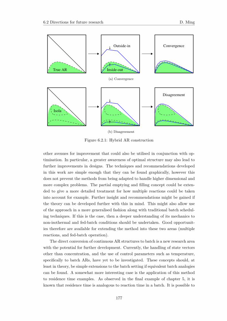
6.2 Directions for future research D. Ming
ConvergenceOutside-in
Inside-outTrue AR
(a) Convergence
Disagreement
Isola
(b) Disagreement
Figure 6.2.1: Hybrid AR construction
other avenues for improvement that could also be utilised in conjunction with op-timisation. In particular, a greater awareness of optimal structure may also lead tofurther improvements in designs. The techniques and recommendations developedin this work are simple enough that they can be found graphically, however thisdoes not prevent the methods from being adapted to handle higher dimensional andmore complex problems. The partial emptying and filling concept could be exten-ded to give a more detailed treatment for how multiple reactions could be takeninto account for example. Further insight and recommendations might be gained ifthe theory can be developed further with this in mind. This might also allow useof the approach in a more generalised fashion along with traditional batch schedul-ing techniques. If this is the case, then a deeper understanding of its mechanics tonon-isothermal and fed-batch conditions should be undertaken. Good opportunit-ies therefore are available for extending the method into these two areas (multiplereactions, and fed-batch operation).
The direct conversion of continuous AR structures to batch is a new research areawith the potential for further development. Currently, the handling of state vectorsother than concentration, and the use of control parameters such as temperature,specifically to batch ARs, have yet to be investigated. These concepts should, atleast in theory, be simple extensions to the batch setting if equivalent batch analogiescan be found. A somewhat more interesting case is the application of this methodto residence time examples. As observed in the final example of chapter 5, it isknown that residence time is analogous to reaction time in a batch. It is possible to
177
6.2 Directions for future research D. Ming
mix residence time, but the same clearly does not translate to batch using reactiontime. Chapter 3 is dedicated to batch production rate, and so there is a connectionbetween the simple recommendations given to the larger picture of AR residence timeexamples. It may turn out that when converting continuous AR structures to batchusing residence time constructions, greater benefit might be obtained if flow rate andvolume are considered, rather than simply residence time alone. Understanding thisrelation might allow for the conversion of more complicated residence time ARs tobatch. Consequently, higher dimensional problems in batch could also be addressedif some of the questions posed above are given attention.
We note that along with the idea of a hybrid approach to AR construction, therealso exists another hybrid approach specific to batch reactors. That is, along withthe developments of AR theory to batch reactors, this methodology could also beincorporated into more generalised batch structures involving other batch processingequipment. Opportunities for further research exists that investigates improvementsto batch reactors by combining AR theory concepts into batch process schedul-ing policies. Specifically, the AR could be combined with non-linear programmingstrategies and used as an initialisation for these methods – if it is known that aparticular state is achievable within the reactive portion of the batch network, thenthis allows for rapid iteration to a final, optimal batch schedule using AR theory.It would be useful to understand, from a scheduling perspective, that, within thereactive portion of the batch plant, a specific product can be delivered within acertain quality specification (yield, waste minimisation, conversion, etc.), within acycle time (residence time or reactor volume), under the operating constraints of theplant. Knowing this might open up further avenues for batch improvement as nowthe designer is knowledgeable of the absolute limits of rector section of the plant.This knowledge may be useful for highly complex batch process optimizations; ARtheory helps us to understand the details inside the reactor network. The combin-ation of ARs with generalised batch equipment is an interesting concept that hasnot yet been explored, but which may offer powerful insights into batch processimprovements in general.
Final remarks
Although the current landscape of AR research is not vast, particularly when con-sidered against other fields far more established (and popular) than that consideredhere, this should not be interpreted as a field that is by any means complete. Ifanything, this would suggest that the field is still in its infancy. There remains agreat deal of unknown to the theories developed in AR (and yet to be developed),and their relation to a sufficiency condition. The challenges in AR stem from threemain areas of concern:
1. Accurate and efficient AR construction.
178

6.2 Directions for future research D. Ming
2. A low adoption of the method within the process engineering community.
3. And a relatively limited theory base on what is actually known about the AR.
It is my hope that progress in AR will continue to be made with these issues inmind.
With developments of new ideas and the expansion of the profession into broaderfields of work, process engineers find use working in industries that would histor-ically not have been considered in the past. The training and methods developedin traditional areas of practice will thus need to find use under different fields ofapplication. There exists a great need to continue developing topics in chemicalengineering that can then be transferred, translated and adapted to new areas ofexpertise.
179
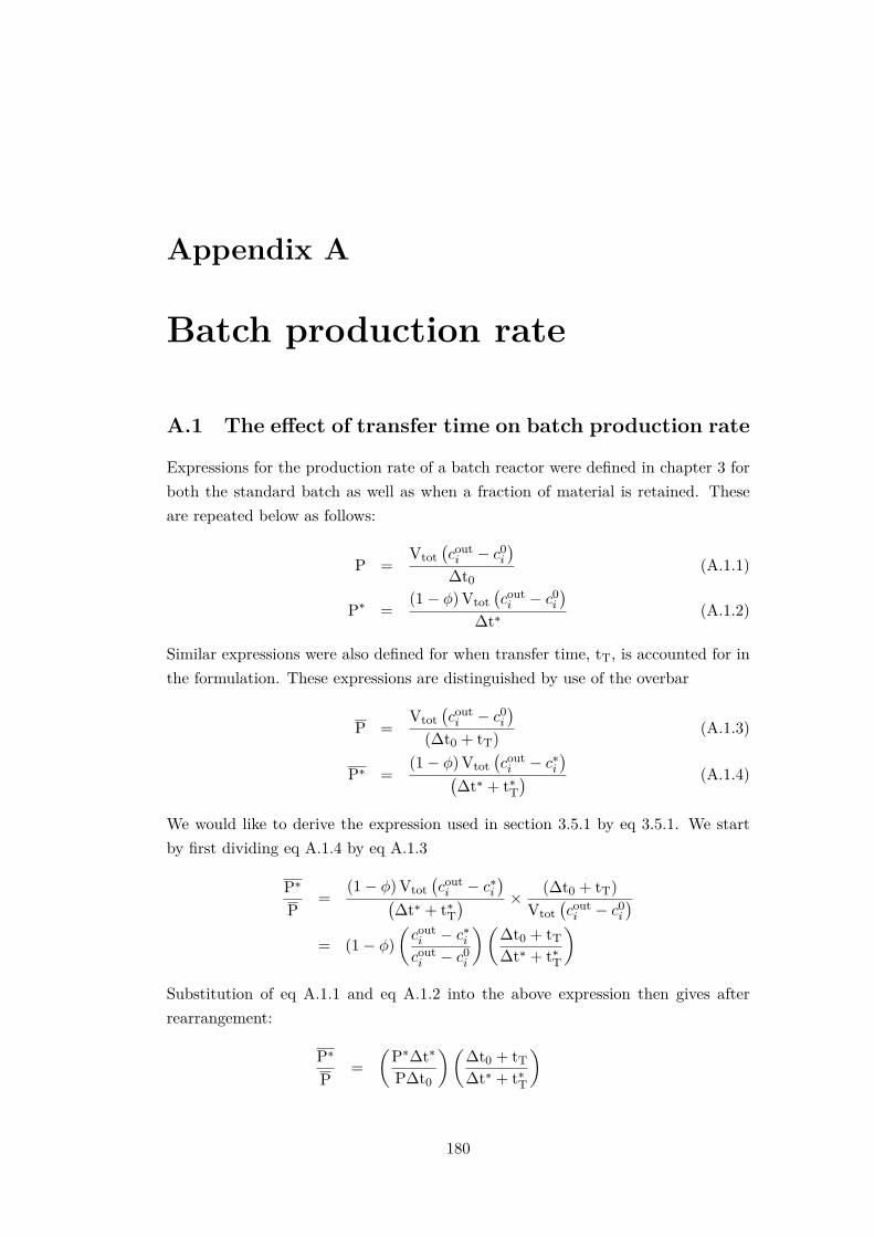
Appendix A
Batch production rate
A.1 The effect of transfer time on batch production rate
Expressions for the production rate of a batch reactor were defined in chapter 3 forboth the standard batch as well as when a fraction of material is retained. Theseare repeated below as follows:
P =Vtot
(couti − c0i
)∆t0
(A.1.1)
P∗ =(1− ϕ)Vtot
(couti − c0i
)∆t∗ (A.1.2)
Similar expressions were also defined for when transfer time, tT, is accounted for inthe formulation. These expressions are distinguished by use of the overbar
P =Vtot
(couti − c0i
)(∆t0 + tT)
(A.1.3)
P∗ =(1− ϕ)Vtot
(couti − c∗i
)(∆t∗ + t∗T
) (A.1.4)
We would like to derive the expression used in section 3.5.1 by eq 3.5.1. We startby first dividing eq A.1.4 by eq A.1.3
P∗
P=
(1− ϕ)Vtot(couti − c∗i
)(∆t∗ + t∗T
) × (∆t0 + tT)
Vtot(couti − c0i
)= (1− ϕ)
(couti − c∗icouti − c0i
)(∆t0 + tT∆t∗ + t∗T
)Substitution of eq A.1.1 and eq A.1.2 into the above expression then gives afterrearrangement:
P∗
P=
(P∗∆t∗P∆t0
)(∆t0 + tT∆t∗ + t∗T
)
180
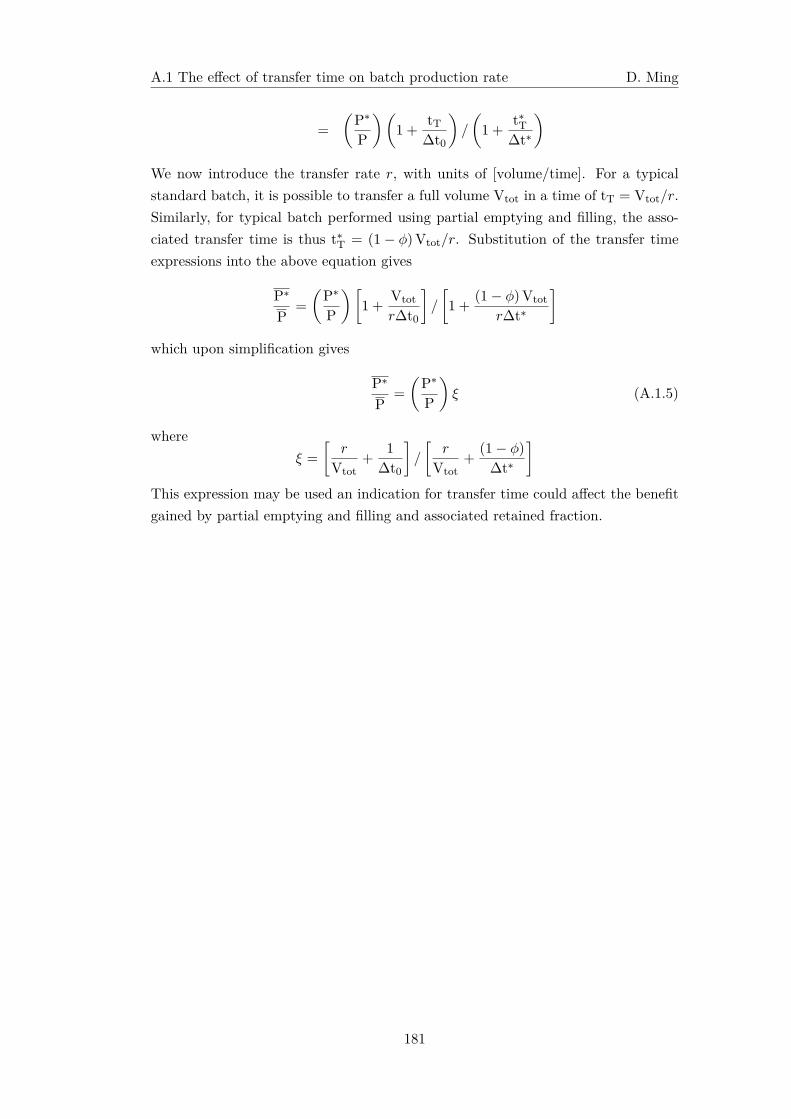
A.1 The effect of transfer time on batch production rate D. Ming
=
(P∗
P
)(1 +
tT∆t0
)/
(1 +
t∗T∆t∗
)We now introduce the transfer rate r, with units of [volume/time]. For a typicalstandard batch, it is possible to transfer a full volume Vtot in a time of tT = Vtot/r.Similarly, for typical batch performed using partial emptying and filling, the asso-ciated transfer time is thus t∗T = (1− ϕ)Vtot/r. Substitution of the transfer timeexpressions into the above equation gives
P∗
P=
(P∗
P
)[1 +
Vtotr∆t0
]/
[1 +
(1− ϕ)Vtotr∆t∗
]which upon simplification gives
P∗
P=
(P∗
P
)ξ (A.1.5)
whereξ =
[r
Vtot+
1
∆t0
]/
[r
Vtot+
(1− ϕ)
∆t∗
]This expression may be used an indication for transfer time could affect the benefitgained by partial emptying and filling and associated retained fraction.
181
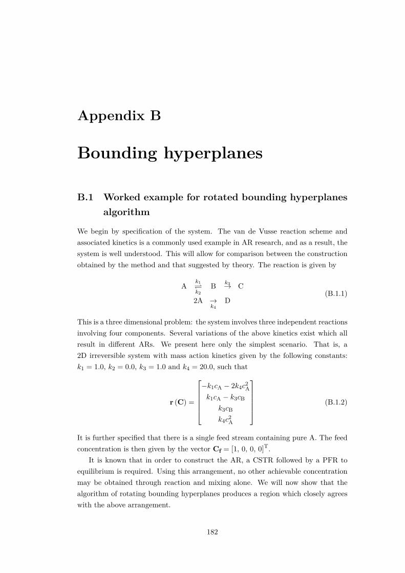
Appendix B
Bounding hyperplanes
B.1 Worked example for rotated bounding hyperplanesalgorithm
We begin by specification of the system. The van de Vusse reaction scheme andassociated kinetics is a commonly used example in AR research, and as a result, thesystem is well understood. This will allow for comparison between the constructionobtained by the method and that suggested by theory. The reaction is given by
Ak1k2
B k3→ C
2A →k4
D(B.1.1)
This is a three dimensional problem: the system involves three independent reactionsinvolving four components. Several variations of the above kinetics exist which allresult in different ARs. We present here only the simplest scenario. That is, a2D irreversible system with mass action kinetics given by the following constants:k1 = 1.0, k2 = 0.0, k3 = 1.0 and k4 = 20.0, such that
r (C) =
−k1cA − 2k4c
2A
k1cA − k3cB
k3cB
k4c2A
(B.1.2)
It is further specified that there is a single feed stream containing pure A. The feedconcentration is then given by the vector Cf = [1, 0, 0, 0]T.
It is known that in order to construct the AR, a CSTR followed by a PFR toequilibrium is required. Using this arrangement, no other achievable concentrationmay be obtained through reaction and mixing alone. We will now show that thealgorithm of rotating bounding hyperplanes produces a region which closely agreeswith the above arrangement.
182
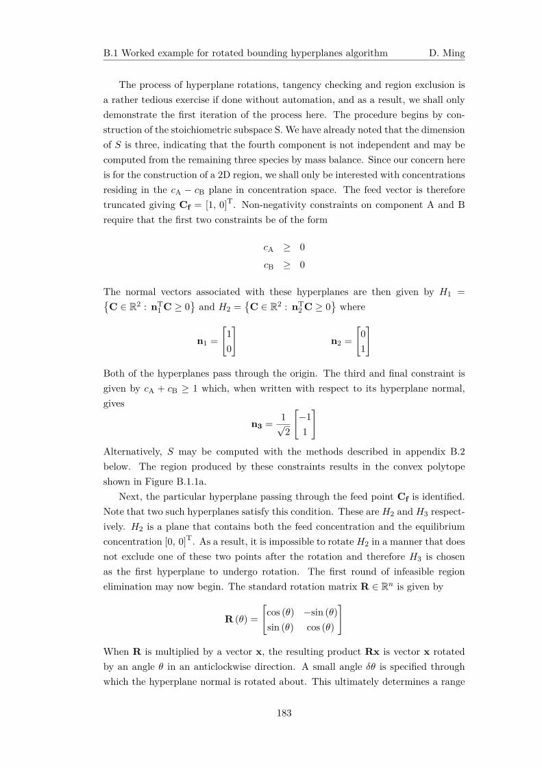
B.1 Worked example for rotated bounding hyperplanes algorithm D. Ming
The process of hyperplane rotations, tangency checking and region exclusion isa rather tedious exercise if done without automation, and as a result, we shall onlydemonstrate the first iteration of the process here. The procedure begins by con-struction of the stoichiometric subspace S. We have already noted that the dimensionof S is three, indicating that the fourth component is not independent and may becomputed from the remaining three species by mass balance. Since our concern hereis for the construction of a 2D region, we shall only be interested with concentrationsresiding in the cA − cB plane in concentration space. The feed vector is thereforetruncated giving Cf = [1, 0]T. Non-negativity constraints on component A and Brequire that the first two constraints be of the form
cA ≥ 0
cB ≥ 0
The normal vectors associated with these hyperplanes are then given by H1 ={C ∈ R2 : nT
1 C ≥ 0}
and H2 ={
C ∈ R2 : nT2 C ≥ 0
}where
n1 =
[1
0
]n2 =
[0
1
]
Both of the hyperplanes pass through the origin. The third and final constraint isgiven by cA + cB ≥ 1 which, when written with respect to its hyperplane normal,gives
n3 =1√2
[−1
1
]Alternatively, S may be computed with the methods described in appendix B.2below. The region produced by these constraints results in the convex polytopeshown in Figure B.1.1a.
Next, the particular hyperplane passing through the feed point Cf is identified.Note that two such hyperplanes satisfy this condition. These are H2 and H3 respect-ively. H2 is a plane that contains both the feed concentration and the equilibriumconcentration [0, 0]T. As a result, it is impossible to rotate H2 in a manner that doesnot exclude one of these two points after the rotation and therefore H3 is chosenas the first hyperplane to undergo rotation. The first round of infeasible regionelimination may now begin. The standard rotation matrix R ∈ Rn is given by
R (θ) =
[cos (θ) −sin (θ)
sin (θ) cos (θ)
]
When R is multiplied by a vector x, the resulting product Rx is vector x rotatedby an angle θ in an anticlockwise direction. A small angle δθ is specified throughwhich the hyperplane normal is rotated about. This ultimately determines a range
183
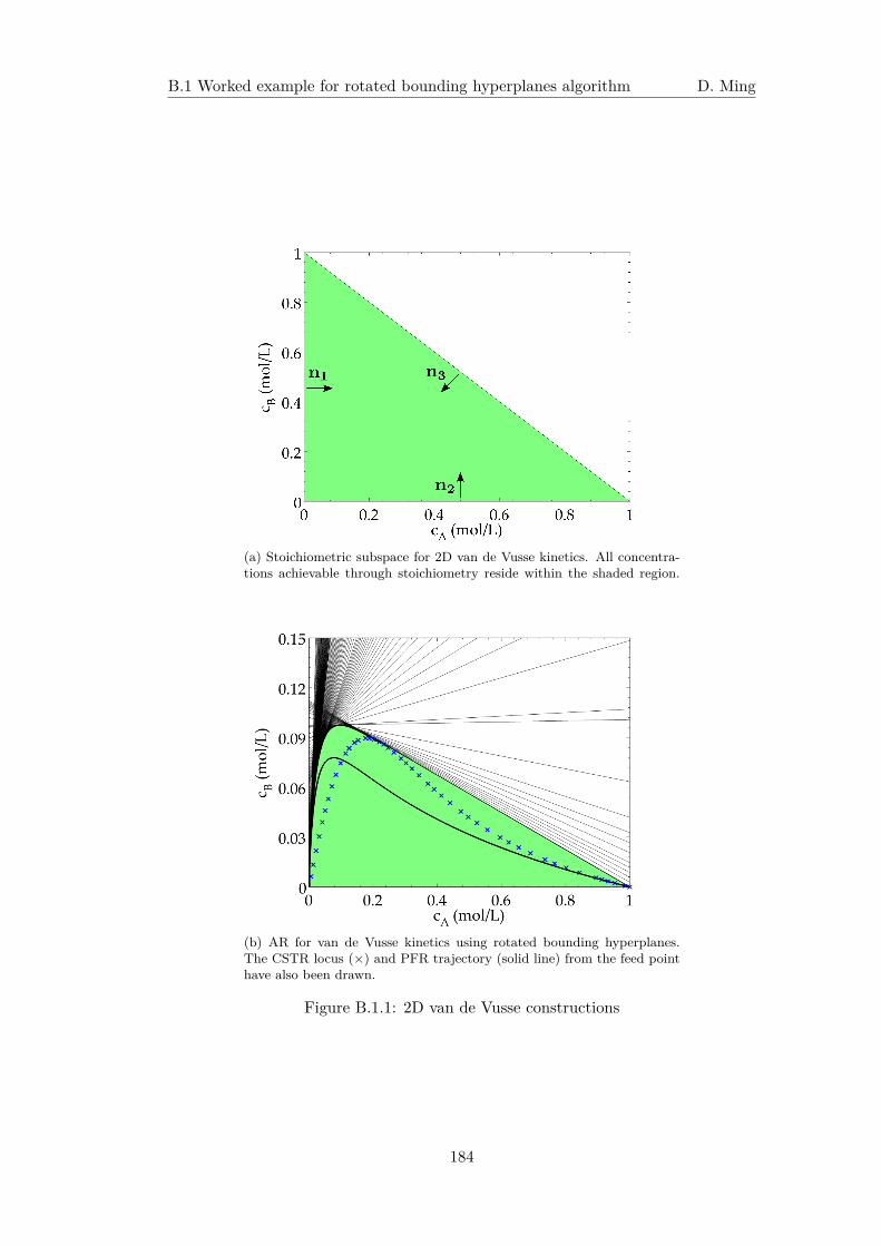
B.1 Worked example for rotated bounding hyperplanes algorithm D. Ming
(a) Stoichiometric subspace for 2D van de Vusse kinetics. All concentra-tions achievable through stoichiometry reside within the shaded region.
(b) AR for van de Vusse kinetics using rotated bounding hyperplanes.The CSTR locus (×) and PFR trajectory (solid line) from the feed pointhave also been drawn.
Figure B.1.1: 2D van de Vusse constructions
184
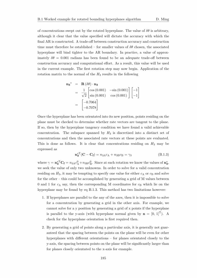
B.1 Worked example for rotated bounding hyperplanes algorithm D. Ming
of concentrations swept out by the rotated hyperplane. The value of δθ is arbitrary,although it clear that the value specified will dictate the accuracy with which thefinal AR is constructed. A trade-off between construction accuracy and constructiontime must therefore be established – for smaller values of δθ chosen, the associatedhyperplane will bind tighter to the AR boundary. In practice, a value of approx-imately δθ = 0.001 radians has been found to be an adequate trade-off betweenconstruction accuracy and computational effort. As a result, this value will be usedin the current example. The first rotation step may now begin. Application of therotation matrix to the normal of the H3 results in the following
n3∗ = R (δθ) · n3
=1√2
[cos (0.001) −sin (0.001)sin (0.001) cos (0.001)
][−1
−1
]
=
[−0.7064
−0.7078
]
Once the hyperplane has been orientated into its new position, points residing on theplane must be checked to determine whether rate vectors are tangent to the plane.If so, then by the hyperplane tangency condition we have found a valid achievableconcentration. The subspace spanned by H3 is discretised into a distinct set ofconcentrations and then the associated rate vectors at these points are evaluated.This is done as follows. It is clear that concentrations residing on H3 may beexpressed as
n∗T3 (C − Cf) = n3AcA + n3BcB = γ3 (B.1.3)
where γ = n∗T3 Cf = n3Ac
0A+n3Bc0B. Since at each rotation we know the values of n∗
3,we seek the value of only two unknowns. In order to solve for a valid concentrationresiding on H3, it may be tempting to specify one value for either cA or cB and solvefor the other – this could be accomplished by generating a grid of M values between0 and 1 for cA say, then the corresponding M coordinates for cB which lie on thehyperplane may be found by eq B.1.3. This method has two limitations however:
1. If hyperplanes are parallel to the any of the axes, then it is impossible to solvefor a concentration by generating a grid in the other axis. For example, wecannot solve for a y position by generating a grid of x points if the hyperplaneis parallel to the y-axis (with hyperplane normal given by n = [0, 1]T). Acheck for the hyperplane orientation is first required then.
2. By generating a grid of points along a particular axis, it is generally not guar-anteed that the spacing between the points on the plane will be even for otherhyperplanes with different orientations – for planes orientated closely to they-axis, the spacing between points on the plane will be significantly larger thanfor planes closely orientated to the x-axis for example.
185
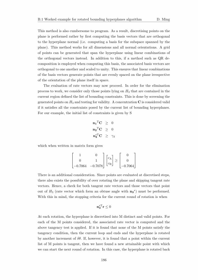
B.1 Worked example for rotated bounding hyperplanes algorithm D. Ming
This method is also cumbersome to program. As a result, discretising points on theplane is performed rather by first computing the basis vectors that are orthogonalto the hyperplane normal (i.e. computing a basis for the subspace spanned by theplane). This method works for all dimensions and all normal orientations. A gridof points can be generated that span the hyperplane using linear combinations ofthe orthogonal vectors instead. In addition to this, if a method such as QR de-composition is employed when computing this basis, the associated basis vectors areorthogonal to one another and scaled to unity. This ensures that linear combinationsof the basis vectors generate points that are evenly spaced on the plane irrespectiveof the orientation of the plane itself in space.
The evaluation of rate vectors may now proceed. In order for the eliminationprocess to work, we consider only those points lying on H3 that are contained in thecurrent region defined the list of bounding constraints. This is done by screening thegenerated points on H3 and testing for validity. A concentration C is considered validif it satisfies all the constraints posed by the current list of bounding hyperplanes.For our example, the initial list of constraints is given by S
n1TC ≥ 0
n2TC ≥ 0
n∗T3 C ≥ γ3
which when written in matrix form gives 1 0
0 1
−0.7064 −0.7078
[cA
cB
]≥
0
0
−0.7064
There is an additional consideration. Since points are evaluated at discretised steps,there also exists the possibility of over rotating the plane and skipping tangent ratevectors. Hence, a check for both tangent rate vectors and those vectors that pointout of H3 (rate vector which form an obtuse angle with n3∗) must be performed.With this in mind, the stopping criteria for the current round of rotation is when
n∗T3 r ≤ 0
At each rotation, the hyperplane is discretised into M distinct and valid points. Foreach of the M points considered, the associated rate vector is computed and theabove tangency test is applied. If it is found that none of the M points satisfy thetangency condition, then the current loop and ends and the hyperplane is rotatedby another increment of δθ. If, however, it is found that a point within the currentlist of M points is tangent, then we have found a new attainable point with whichwe can start the next round of rotation. In this case, the hyperplane is rotated back
186
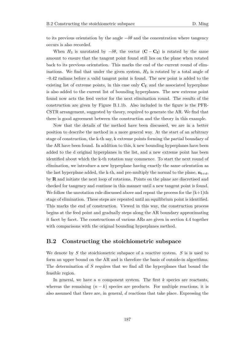
B.2 Constructing the stoichiometric subspace D. Ming
to its previous orientation by the angle −δθ and the concentration where tangencyoccurs is also recorded.
When H3 is unrotated by −δθ, the vector (C − Cf) is rotated by the sameamount to ensure that the tangent point found still lies on the plane when rotatedback to its previous orientation. This marks the end of the current round of elim-inations. We find that under the given system, H3 is rotated by a total angle of~0.42 radians before a valid tangent point is found. The new point is added to theexisting list of extreme points, in this case only Cf, and the associated hyperplaneis also added to the current list of bounding hyperplanes. The new extreme pointfound now acts the feed vector for the next elimination round. The results of theconstruction are given by Figure B.1.1b. Also included in the figure is the PFR-CSTR arrangement, suggested by theory, required to generate the AR. We find thatthere is good agreement between the construction and the theory in this example.
Now that the details of the method have been discussed, we are in a betterposition to describe the method in a more general way. At the start of an arbitrarystage of construction, the k-th say, k extreme points forming the partial boundary ofthe AR have been found. In addition to this, k new bounding hyperplanes have beenadded to the d original hyperplanes in the list, and a new extreme point has beenidentified about which the k-th rotation may commence. To start the next round ofelimination, we introduce a new hyperplane having exactly the same orientation asthe last hyperplane added, the k-th, and pre-multiply the normal to the plane, nk+d,by R and initiate the next loop of rotations. Points on the plane are discretised andchecked for tangency and continue in this manner until a new tangent point is found.We follow the unrotation rule discussed above and repeat the process for the (k+1)thstage of elimination. These steps are repeated until an equilibrium point is identified.This marks the end of construction. Viewed in this way, the construction processbegins at the feed point and gradually steps along the AR boundary approximatingit facet by facet. The constructions of various ARs are given in section 4.4 togetherwith comparisons with the original bounding hyperplanes method.
B.2 Constructing the stoichiometric subspace
We denote by S the stoichiometric subspace of a reactive system. S is is used toform an upper bound on the AR and is therefore the basis of outside-in algorithms.The determination of S requires that we find all the hyperplanes that bound thefeasible region.
In general, we have a n component system. The first k species are reactants,whereas the remaining (n− k) species are products. For multiple reactions, it isalso assumed that there are, in general, d reactions that take place. Expressing the
187
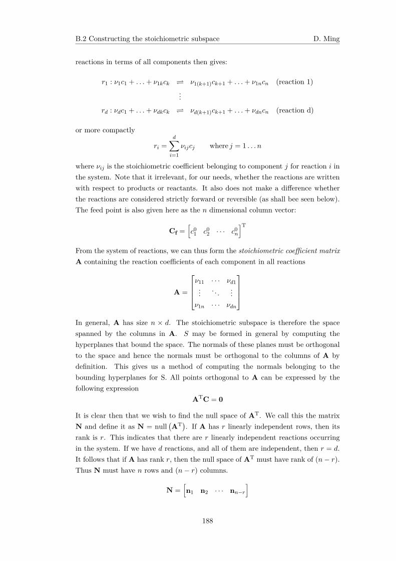
B.2 Constructing the stoichiometric subspace D. Ming
reactions in terms of all components then gives:
r1 : ν1c1 + . . .+ ν1kck ν1(k+1)ck+1 + . . .+ ν1ncn (reaction 1)...
rd : νdc1 + . . .+ νdkck νd(k+1)ck+1 + . . .+ νdncn (reaction d)
or more compactly
ri =
d∑i=1
νijcj where j = 1 . . . n
where νij is the stoichiometric coefficient belonging to component j for reaction i inthe system. Note that it irrelevant, for our needs, whether the reactions are writtenwith respect to products or reactants. It also does not make a difference whetherthe reactions are considered strictly forward or reversible (as shall bee seen below).The feed point is also given here as the n dimensional column vector:
Cf =[c01 c02 · · · c0n
]T
From the system of reactions, we can thus form the stoichiometric coefficient matrixA containing the reaction coefficients of each component in all reactions
A =
ν11 · · · νd1... . . . ...
ν1n · · · νdn
In general, A has size n × d. The stoichiometric subspace is therefore the spacespanned by the columns in A. S may be formed in general by computing thehyperplanes that bound the space. The normals of these planes must be orthogonalto the space and hence the normals must be orthogonal to the columns of A bydefinition. This gives us a method of computing the normals belonging to thebounding hyperplanes for S. All points orthogonal to A can be expressed by thefollowing expression
ATC = 0
It is clear then that we wish to find the null space of AT. We call this the matrixN and define it as N = null
(AT). If A has r linearly independent rows, then its
rank is r. This indicates that there are r linearly independent reactions occurringin the system. If we have d reactions, and all of them are independent, then r = d.It follows that if A has rank r, then the null space of AT must have rank of (n− r).Thus N must have n rows and (n− r) columns.
N =[n1 n2 · · · nn−r
]
188
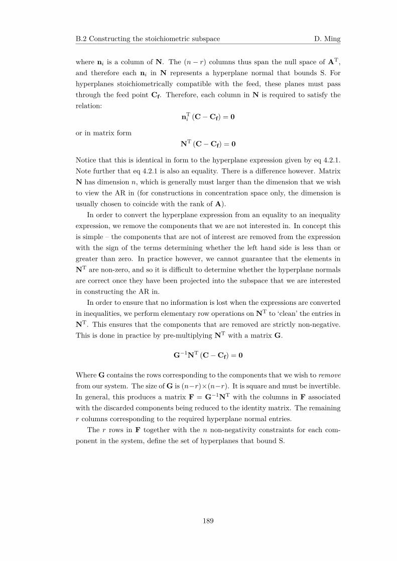
B.2 Constructing the stoichiometric subspace D. Ming
where ni is a column of N. The (n− r) columns thus span the null space of AT,and therefore each ni in N represents a hyperplane normal that bounds S. Forhyperplanes stoichiometrically compatible with the feed, these planes must passthrough the feed point Cf. Therefore, each column in N is required to satisfy therelation:
nTi (C − Cf) = 0
or in matrix formNT (C − Cf) = 0
Notice that this is identical in form to the hyperplane expression given by eq 4.2.1.Note further that eq 4.2.1 is also an equality. There is a difference however. MatrixN has dimension n, which is generally must larger than the dimension that we wishto view the AR in (for constructions in concentration space only, the dimension isusually chosen to coincide with the rank of A).
In order to convert the hyperplane expression from an equality to an inequalityexpression, we remove the components that we are not interested in. In concept thisis simple – the components that are not of interest are removed from the expressionwith the sign of the terms determining whether the left hand side is less than orgreater than zero. In practice however, we cannot guarantee that the elements inNT are non-zero, and so it is difficult to determine whether the hyperplane normalsare correct once they have been projected into the subspace that we are interestedin constructing the AR in.
In order to ensure that no information is lost when the expressions are convertedin inequalities, we perform elementary row operations on NT to ‘clean’ the entries inNT. This ensures that the components that are removed are strictly non-negative.This is done in practice by pre-multiplying NT with a matrix G.
G−1NT (C − Cf) = 0
Where G contains the rows corresponding to the components that we wish to removefrom our system. The size of G is (n−r)×(n−r). It is square and must be invertible.In general, this produces a matrix F = G−1NT with the columns in F associatedwith the discarded components being reduced to the identity matrix. The remainingr columns corresponding to the required hyperplane normal entries.
The r rows in F together with the n non-negativity constraints for each com-ponent in the system, define the set of hyperplanes that bound S.
189
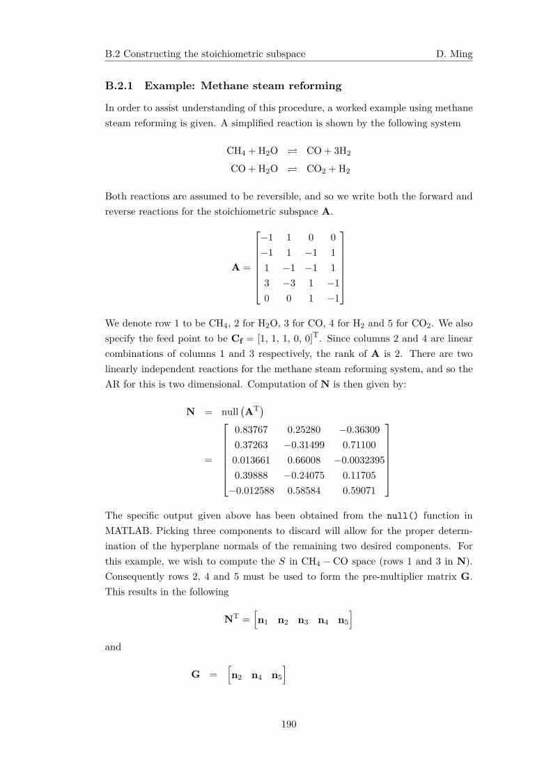
B.2 Constructing the stoichiometric subspace D. Ming
B.2.1 Example: Methane steam reforming
In order to assist understanding of this procedure, a worked example using methanesteam reforming is given. A simplified reaction is shown by the following system
CH4 + H2O CO + 3H2
CO + H2O CO2 + H2
Both reactions are assumed to be reversible, and so we write both the forward andreverse reactions for the stoichiometric subspace A.
A =
−1 1 0 0
−1 1 −1 1
1 −1 −1 1
3 −3 1 −1
0 0 1 −1
We denote row 1 to be CH4, 2 for H2O, 3 for CO, 4 for H2 and 5 for CO2. We alsospecify the feed point to be Cf = [1, 1, 1, 0, 0]T. Since columns 2 and 4 are linearcombinations of columns 1 and 3 respectively, the rank of A is 2. There are twolinearly independent reactions for the methane steam reforming system, and so theAR for this is two dimensional. Computation of N is then given by:
N = null(AT)
=
0.83767 0.25280 −0.36309
0.37263 −0.31499 0.71100
0.013661 0.66008 −0.0032395
0.39888 −0.24075 0.11705
−0.012588 0.58584 0.59071
The specific output given above has been obtained from the null() function inMATLAB. Picking three components to discard will allow for the proper determ-ination of the hyperplane normals of the remaining two desired components. Forthis example, we wish to compute the S in CH4 − CO space (rows 1 and 3 in N).Consequently rows 2, 4 and 5 must be used to form the pre-multiplier matrix G.This results in the following
NT =[n1 n2 n3 n4 n5
]and
G =[n2 n4 n5
]
190
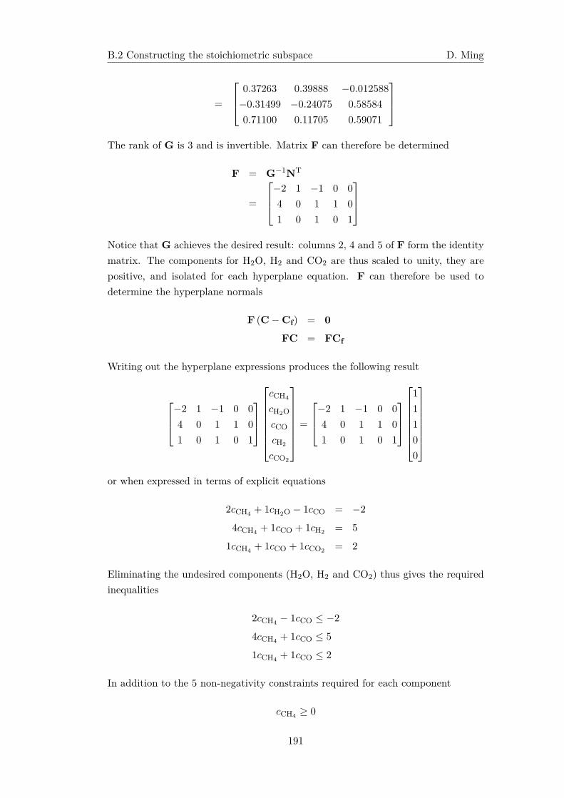
B.2 Constructing the stoichiometric subspace D. Ming
=
0.37263 0.39888 −0.012588
−0.31499 −0.24075 0.58584
0.71100 0.11705 0.59071
The rank of G is 3 and is invertible. Matrix F can therefore be determined
F = G−1NT
=
−2 1 −1 0 0
4 0 1 1 0
1 0 1 0 1
Notice that G achieves the desired result: columns 2, 4 and 5 of F form the identitymatrix. The components for H2O, H2 and CO2 are thus scaled to unity, they arepositive, and isolated for each hyperplane equation. F can therefore be used todetermine the hyperplane normals
F (C − Cf) = 0FC = FCf
Writing out the hyperplane expressions produces the following result
−2 1 −1 0 0
4 0 1 1 0
1 0 1 0 1
cCH4
cH2O
cCO
cH2
cCO2
=
−2 1 −1 0 0
4 0 1 1 0
1 0 1 0 1
1
1
1
0
0
or when expressed in terms of explicit equations
2cCH4 + 1cH2O − 1cCO = −2
4cCH4 + 1cCO + 1cH2 = 5
1cCH4 + 1cCO + 1cCO2 = 2
Eliminating the undesired components (H2O, H2 and CO2) thus gives the requiredinequalities
2cCH4 − 1cCO ≤ −2
4cCH4 + 1cCO ≤ 5
1cCH4 + 1cCO ≤ 2
In addition to the 5 non-negativity constraints required for each component
cCH4 ≥ 0
191
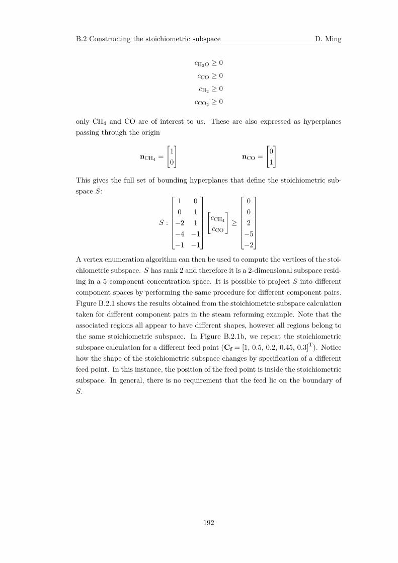
B.2 Constructing the stoichiometric subspace D. Ming
cH2O ≥ 0
cCO ≥ 0
cH2 ≥ 0
cCO2 ≥ 0
only CH4 and CO are of interest to us. These are also expressed as hyperplanespassing through the origin
nCH4 =
[1
0
]nCO =
[0
1
]
This gives the full set of bounding hyperplanes that define the stoichiometric sub-space S:
S :
1 0
0 1
−2 1
−4 −1
−1 −1
[cCH4
cCO
]≥
0
0
2
−5
−2
A vertex enumeration algorithm can then be used to compute the vertices of the stoi-chiometric subspace. S has rank 2 and therefore it is a 2-dimensional subspace resid-ing in a 5 component concentration space. It is possible to project S into differentcomponent spaces by performing the same procedure for different component pairs.Figure B.2.1 shows the results obtained from the stoichiometric subspace calculationtaken for different component pairs in the steam reforming example. Note that theassociated regions all appear to have different shapes, however all regions belong tothe same stoichiometric subspace. In Figure B.2.1b, we repeat the stoichiometricsubspace calculation for a different feed point (Cf = [1, 0.5, 0.2, 0.45, 0.3]T). Noticehow the shape of the stoichiometric subspace changes by specification of a differentfeed point. In this instance, the position of the feed point is inside the stoichiometricsubspace. In general, there is no requirement that the feed lie on the boundary ofS.
192
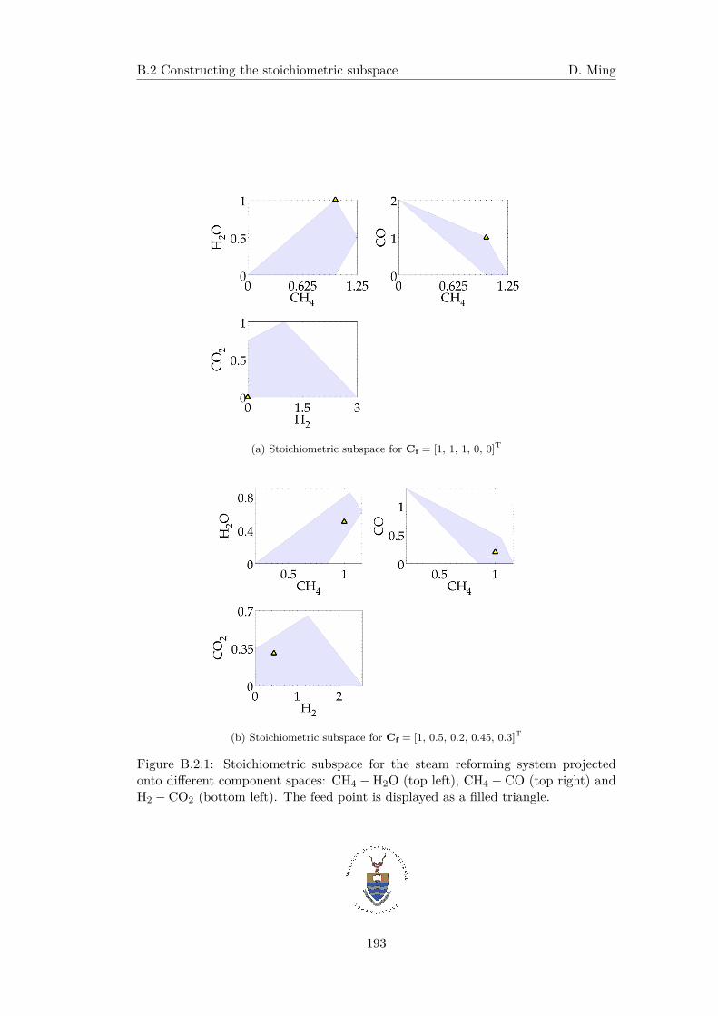
B.2 Constructing the stoichiometric subspace D. Ming
(a) Stoichiometric subspace for Cf = [1, 1, 1, 0, 0]T
(b) Stoichiometric subspace for Cf = [1, 0.5, 0.2, 0.45, 0.3]T
Figure B.2.1: Stoichiometric subspace for the steam reforming system projectedonto different component spaces: CH4 − H2O (top left), CH4 − CO (top right) andH2 − CO2 (bottom left). The feed point is displayed as a filled triangle.
193


![AD-A285 189 I[111] 1j111, INi! 11 II l fll · Examples of such systems include activated sludge, sequential batch reactors, and bioslurry reactors. Treatment of contaminated aquifers](https://img.pdfslide.net/doc/110x75/60567fac99243609c2266269/ad-a285-189-i111-1j111-ini-11-ii-l-fll-examples-of-such-systems-include-activated.jpg)


![International Journal of Pure and Applied Mathematics ...batch/semi batch [6], fixed bed, fluidized bed, spouted bed, microwave [7] and screw kiln. Batch or semi -batch reactors have](https://img.pdfslide.net/doc/110x75/6042d371c8d4a7373d406703/international-journal-of-pure-and-applied-mathematics-batchsemi-batch-6.jpg)