DoctorKnow® Application Paper

Title: Improving Low Frequency Vibration Analysis Source/Author: Richard M. Barrett Product: General Technology: Vibration Classification: Not Classified

IMPROVING LOW FREQUENCY VIBRATION ANALYSIS

Richard M. Barrett, Senior Application Engineer Wilcoxon Research Inc.

CSI 1994 User Conference October 10-14 1994

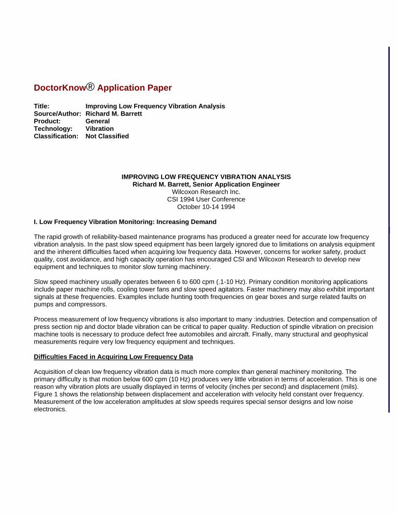
I. Low Frequency Vibration Monitoring: Increasing Demand The rapid growth of reliability-based maintenance programs has produced a greater need for accurate low frequency vibration analysis. In the past slow speed equipment has been largely ignored due to limitations on analysis equipment and the inherent difficulties faced when acquiring low frequency data. However, concerns for worker safety, product quality, cost avoidance, and high capacity operation has encouraged CSI and Wilcoxon Research to develop new equipment and techniques to monitor slow turning machinery. Slow speed machinery usually operates between 6 to 600 cpm (.1-10 Hz). Primary condition monitoring applications include paper machine rolls, cooling tower fans and slow speed agitators. Faster machinery may also exhibit important signals at these frequencies. Examples include hunting tooth frequencies on gear boxes and surge related faults on pumps and compressors. Process measurement of low frequency vibrations is also important to many :industries. Detection and compensation of press section nip and doctor blade vibration can be critical to paper quality. Reduction of spindle vibration on precision machine tools is necessary to produce defect free automobiles and aircraft. Finally, many structural and geophysical measurements require very low frequency equipment and techniques. Difficulties Faced in Acquiring Low Frequency Data Acquisition of clean low frequency vibration data is much more complex than general machinery monitoring. The primary difficulty is that motion below 600 cpm (10 Hz) produces very little vibration in terms of acceleration. This is one reason why vibration plots are usually displayed in terms of velocity (inches per second) and displacement (mils). Figure 1 shows the relationship between displacement and acceleration with velocity held constant over frequency. Measurement of the low acceleration amplitudes at slow speeds requires special sensor designs and low noise electronics.

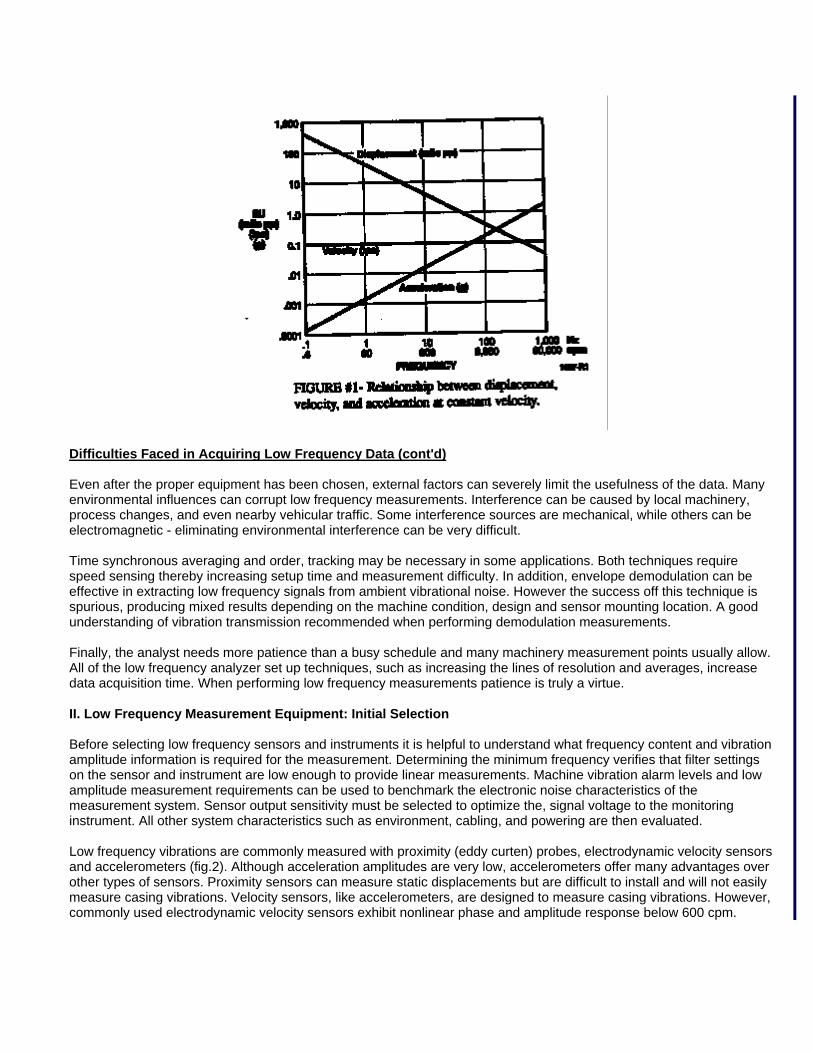
Difficulties Faced in Acquiring Low Frequency Data (cont'd) Even after the proper equipment has been chosen, external factors can severely limit the usefulness of the data. Many environmental influences can corrupt low frequency measurements. Interference can be caused by local machinery, process changes, and even nearby vehicular traffic. Some interference sources are mechanical, while others can be electromagnetic - eliminating environmental interference can be very difficult. Time synchronous averaging and order, tracking may be necessary in some applications. Both techniques require speed sensing thereby increasing setup time and measurement difficulty. In addition, envelope demodulation can be effective in extracting low frequency signals from ambient vibrational noise. However the success off this technique is spurious, producing mixed results depending on the machine condition, design and sensor mounting location. A good understanding of vibration transmission recommended when performing demodulation measurements. Finally, the analyst needs more patience than a busy schedule and many machinery measurement points usually allow. All of the low frequency analyzer set up techniques, such as increasing the lines of resolution and averages, increase data acquisition time. When performing low frequency measurements patience is truly a virtue. II. Low Frequency Measurement Equipment: Initial Selection Before selecting low frequency sensors and instruments it is helpful to understand what frequency content and vibration amplitude information is required for the measurement. Determining the minimum frequency verifies that filter settings on the sensor and instrument are low enough to provide linear measurements. Machine vibration alarm levels and low amplitude measurement requirements can be used to benchmark the electronic noise characteristics of the measurement system. Sensor output sensitivity must be selected to optimize the, signal voltage to the monitoring instrument. All other system characteristics such as environment, cabling, and powering are then evaluated. Low frequency vibrations are commonly measured with proximity (eddy curten) probes, electrodynamic velocity sensors and accelerometers (fig.2). Although acceleration amplitudes are very low, accelerometers offer many advantages over other types of sensors. Proximity sensors can measure static displacements but are difficult to install and will not easily measure casing vibrations. Velocity sensors, like accelerometers, are designed to measure casing vibrations. However, commonly used electrodynamic velocity sensors exhibit nonlinear phase and amplitude response below 600 cpm.

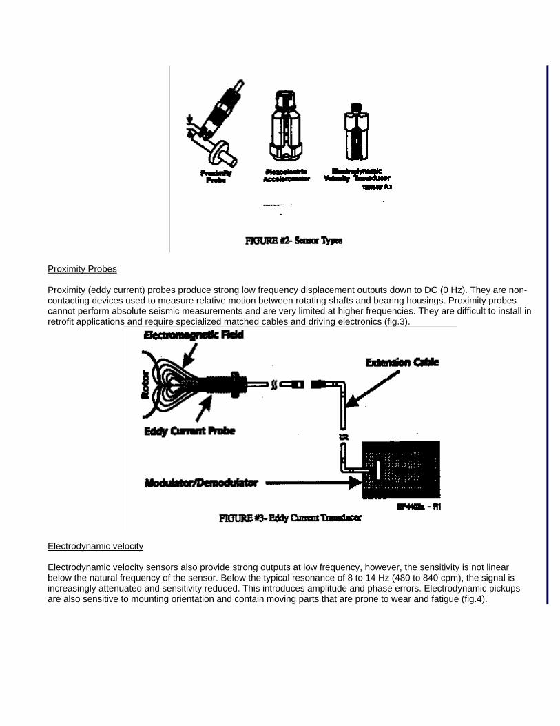
Proximity Probes Proximity (eddy current) probes produce strong low frequency displacement outputs down to DC (0 Hz). They are non-contacting devices used to measure relative motion between rotating shafts and bearing housings. Proximity probes cannot perform absolute seismic measurements and are very limited at higher frequencies. They are difficult to install in retrofit applications and require specialized matched cables and driving electronics (fig.3).

Electrodynamic velocity Electrodynamic velocity sensors also provide strong outputs at low frequency, however, the sensitivity is not linear below the natural frequency of the sensor. Below the typical resonance of 8 to 14 Hz (480 to 840 cpm), the signal is increasingly attenuated and sensitivity reduced. This introduces amplitude and phase errors. Electrodynamic pickups are also sensitive to mounting orientation and contain moving parts that are prone to wear and fatigue (fig.4).

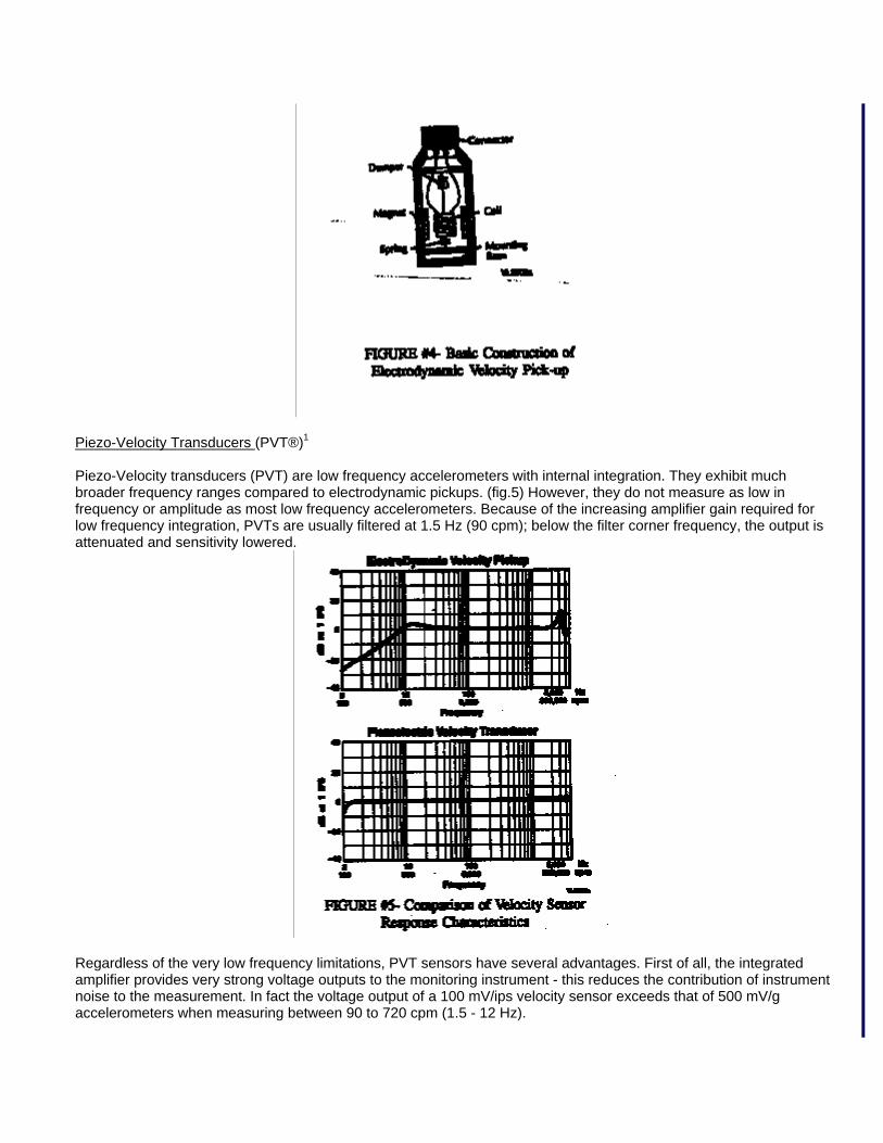
Piezo-Velocity Transducers (PVT®)1 Piezo-Velocity transducers (PVT) are low frequency accelerometers with internal integration. They exhibit much broader frequency ranges compared to electrodynamic pickups. (fig.5) However, they do not measure as low in frequency or amplitude as most low frequency accelerometers. Because of the increasing amplifier gain required for low frequency integration, PVTs are usually filtered at 1.5 Hz (90 cpm); below the filter corner frequency, the output is attenuated and sensitivity lowered.

Regardless of the very low frequency limitations, PVT sensors have several advantages. First of all, the integrated amplifier provides very strong voltage outputs to the monitoring instrument - this reduces the contribution of instrument noise to the measurement. In fact the voltage output of a 100 mV/ips velocity sensor exceeds that of 500 mV/g accelerometers when measuring between 90 to 720 cpm (1.5 - 12 Hz).

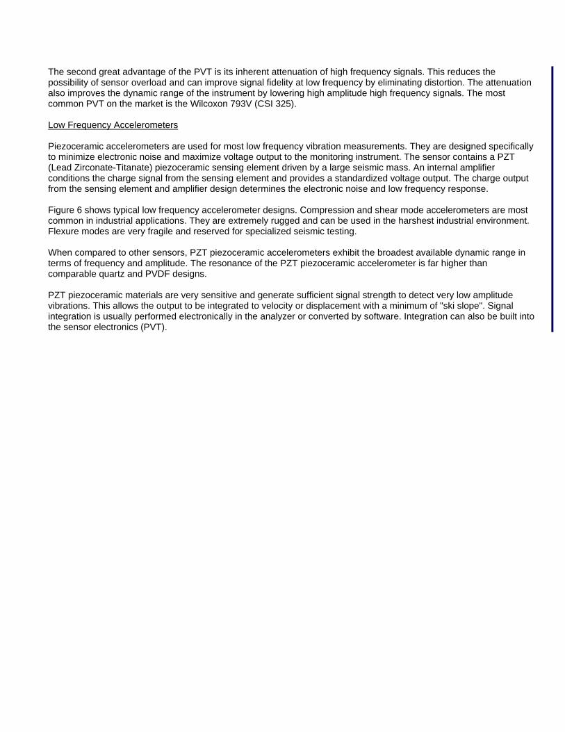
The second great advantage of the PVT is its inherent attenuation of high frequency signals. This reduces the possibility of sensor overload and can improve signal fidelity at low frequency by eliminating distortion. The attenuation also improves the dynamic range of the instrument by lowering high amplitude high frequency signals. The most common PVT on the market is the Wilcoxon 793V (CSI 325). Low Frequency Accelerometers Piezoceramic accelerometers are used for most low frequency vibration measurements. They are designed specifically to minimize electronic noise and maximize voltage output to the monitoring instrument. The sensor contains a PZT (Lead Zirconate-Titanate) piezoceramic sensing element driven by a large seismic mass. An internal amplifier conditions the charge signal from the sensing element and provides a standardized voltage output. The charge output from the sensing element and amplifier design determines the electronic noise and low frequency response. Figure 6 shows typical low frequency accelerometer designs. Compression and shear mode accelerometers are most common in industrial applications. They are extremely rugged and can be used in the harshest industrial environment. Flexure modes are very fragile and reserved for specialized seismic testing. When compared to other sensors, PZT piezoceramic accelerometers exhibit the broadest available dynamic range in terms of frequency and amplitude. The resonance of the PZT piezoceramic accelerometer is far higher than comparable quartz and PVDF designs. PZT piezoceramic materials are very sensitive and generate sufficient signal strength to detect very low amplitude vibrations. This allows the output to be integrated to velocity or displacement with a minimum of "ski slope". Signal integration is usually performed electronically in the analyzer or converted by software. Integration can also be built into the sensor electronics (PVT).

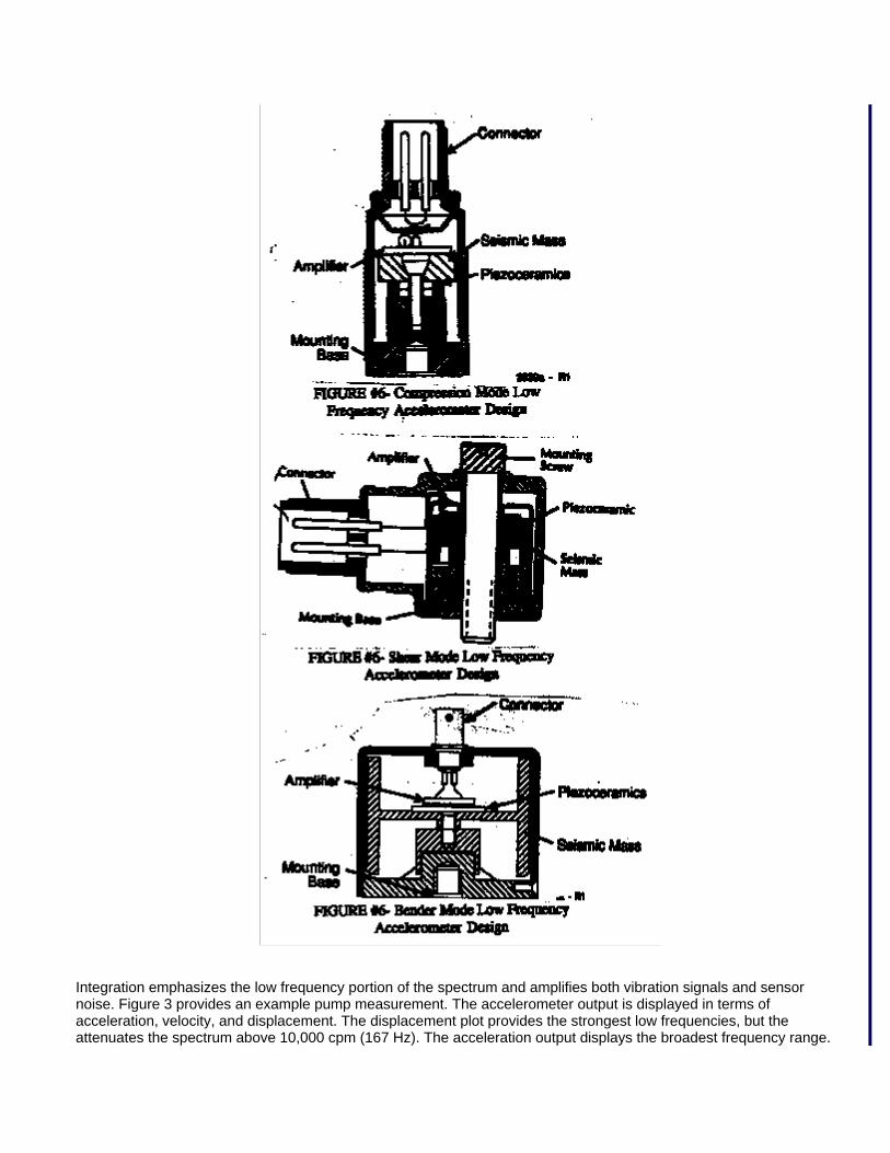
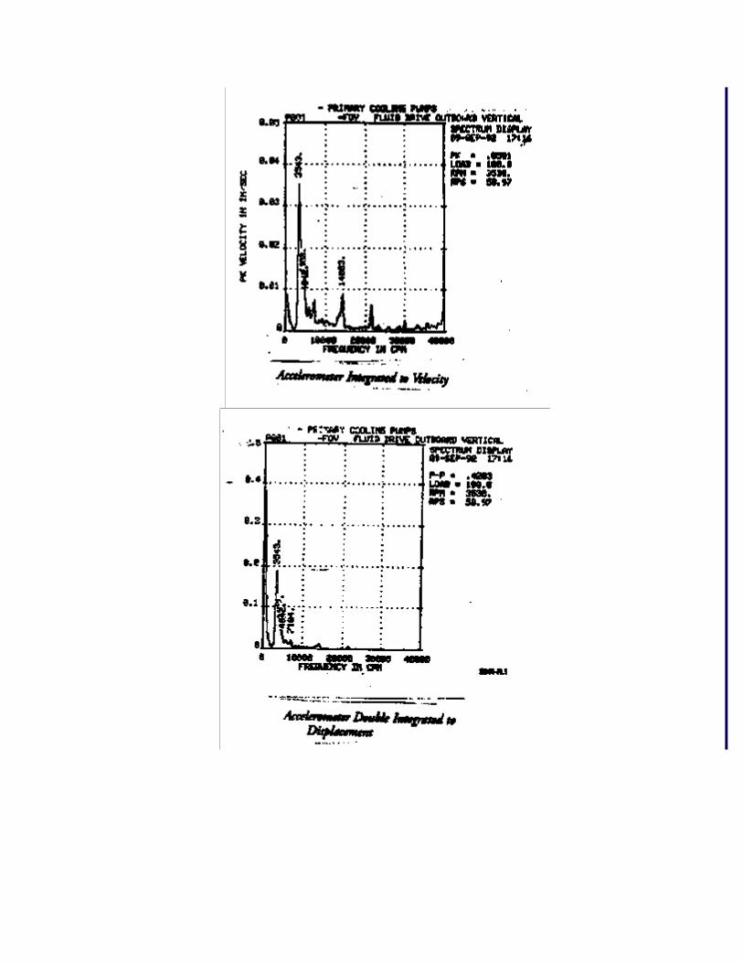
Integration emphasizes the low frequency portion of the spectrum and amplifies both vibration signals and sensor noise. Figure 3 provides an example pump measurement. The accelerometer output is displayed in terms of acceleration, velocity, and displacement. The displacement plot provides the strongest low frequencies, but the attenuates the spectrum above 10,000 cpm (167 Hz). The acceleration output displays the broadest frequency range.

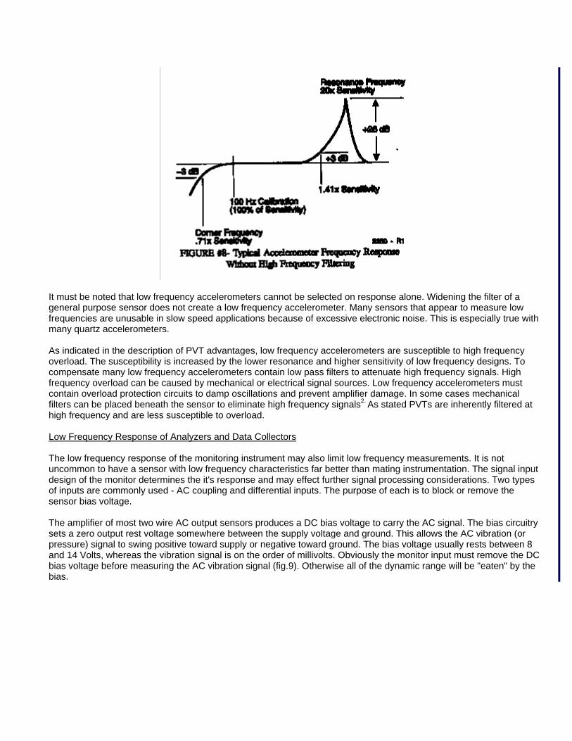
III. Low Frequency Response of the Measurement System The low frequency response of piezoelectric accelerometers and most measurement instruments do not extend to DC (0Hz). All charge amplifiers for accelerometer contain filters at low frequencies. Measurement equipment must also contain filters or some other method to block the bias voltage of the accelerometer. When selecting a sensor and analyzer (or dam collector, DAT recorder etc.), the low frequency response of the system must be evaluated. Accelerometer Filtering Piezoelectric sensors use high pass filters to remove DC and near DC signals (fig.8). Filtering eliminates low frequency transients caused by thermal or swain expansion of the sensor housing. The filter corner frequency defines the point at which the sensitivity is attenuated to 71% (-3dB) of the calibrated sensitivity (500 mV/g, 100 mV/ips, etc.). Below the corner frequency of a single pole filter, the signal will be reduced by half every time the frequency is halved. If a 2 pole filter is used it will be reduced to one fourth every time the frequency is cut in half.

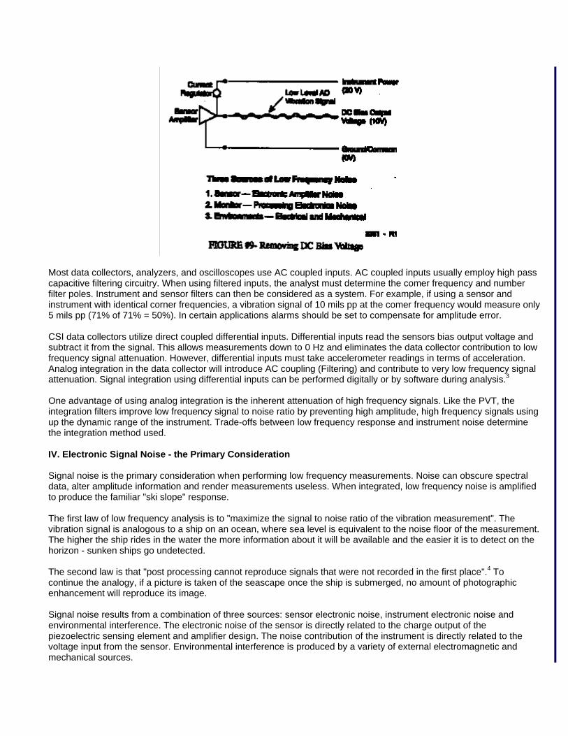
It must be noted that low frequency accelerometers cannot be selected on response alone. Widening the filter of a general purpose sensor does not create a low frequency accelerometer. Many sensors that appear to measure low frequencies are unusable in slow speed applications because of excessive electronic noise. This is especially true with many quartz accelerometers. As indicated in the description of PVT advantages, low frequency accelerometers are susceptible to high frequency overload. The susceptibility is increased by the lower resonance and higher sensitivity of low frequency designs. To compensate many low frequency accelerometers contain low pass filters to attenuate high frequency signals. High frequency overload can be caused by mechanical or electrical signal sources. Low frequency accelerometers must contain overload protection circuits to damp oscillations and prevent amplifier damage. In some cases mechanical filters can be placed beneath the sensor to eliminate high frequency signals2. As stated PVTs are inherently filtered at high frequency and are less susceptible to overload. Low Frequency Response of Analyzers and Data Collectors The low frequency response of the monitoring instrument may also limit low frequency measurements. It is not uncommon to have a sensor with low frequency characteristics far better than mating instrumentation. The signal input design of the monitor determines the it's response and may effect further signal processing considerations. Two types of inputs are commonly used - AC coupling and differential inputs. The purpose of each is to block or remove the sensor bias voltage. The amplifier of most two wire AC output sensors produces a DC bias voltage to carry the AC signal. The bias circuitry sets a zero output rest voltage somewhere between the supply voltage and ground. This allows the AC vibration (or pressure) signal to swing positive toward supply or negative toward ground. The bias voltage usually rests between 8 and 14 Volts, whereas the vibration signal is on the order of millivolts. Obviously the monitor input must remove the DC bias voltage before measuring the AC vibration signal (fig.9). Otherwise all of the dynamic range will be "eaten" by the bias.

Most data collectors, analyzers, and oscilloscopes use AC coupled inputs. AC coupled inputs usually employ high pass capacitive filtering circuitry. When using filtered inputs, the analyst must determine the comer frequency and number filter poles. Instrument and sensor filters can then be considered as a system. For example, if using a sensor and instrument with identical corner frequencies, a vibration signal of 10 mils pp at the comer frequency would measure only 5 mils pp (71% of 71% = 50%). In certain applications alarms should be set to compensate for amplitude error. CSI data collectors utilize direct coupled differential inputs. Differential inputs read the sensors bias output voltage and subtract it from the signal. This allows measurements down to 0 Hz and eliminates the data collector contribution to low frequency signal attenuation. However, differential inputs must take accelerometer readings in terms of acceleration. Analog integration in the data collector will introduce AC coupling (Filtering) and contribute to very low frequency signal attenuation. Signal integration using differential inputs can be performed digitally or by software during analysis.3 One advantage of using analog integration is the inherent attenuation of high frequency signals. Like the PVT, the integration filters improve low frequency signal to noise ratio by preventing high amplitude, high frequency signals using up the dynamic range of the instrument. Trade-offs between low frequency response and instrument noise determine the integration method used. IV. Electronic Signal Noise - the Primary Consideration Signal noise is the primary consideration when performing low frequency measurements. Noise can obscure spectral data, alter amplitude information and render measurements useless. When integrated, low frequency noise is amplified to produce the familiar "ski slope" response. The first law of low frequency analysis is to "maximize the signal to noise ratio of the vibration measurement". The vibration signal is analogous to a ship on an ocean, where sea level is equivalent to the noise floor of the measurement. The higher the ship rides in the water the more information about it will be available and the easier it is to detect on the horizon - sunken ships go undetected. The second law is that "post processing cannot reproduce signals that were not recorded in the first place".4 To continue the analogy, if a picture is taken of the seascape once the ship is submerged, no amount of photographic enhancement will reproduce its image. Signal noise results from a combination of three sources: sensor electronic noise, instrument electronic noise and environmental interference. The electronic noise of the sensor is directly related to the charge output of the piezoelectric sensing element and amplifier design. The noise contribution of the instrument is directly related to the voltage input from the sensor. Environmental interference is produced by a variety of external electromagnetic and mechanical sources.

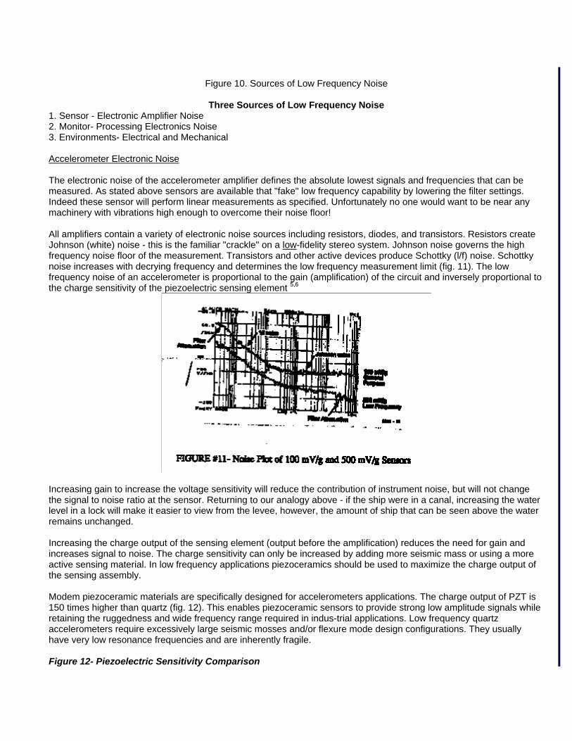
Figure 10. Sources of Low Frequency Noise

Three Sources of Low Frequency Noise

1. Sensor - Electronic Amplifier Noise 2. Monitor- Processing Electronics Noise 3. Environments- Electrical and Mechanical Accelerometer Electronic Noise The electronic noise of the accelerometer amplifier defines the absolute lowest signals and frequencies that can be measured. As stated above sensors are available that "fake" low frequency capability by lowering the filter settings. Indeed these sensor will perform linear measurements as specified. Unfortunately no one would want to be near any machinery with vibrations high enough to overcome their noise floor! All amplifiers contain a variety of electronic noise sources including resistors, diodes, and transistors. Resistors create Johnson (white) noise - this is the familiar "crackle" on a low-fidelity stereo system. Johnson noise governs the high frequency noise floor of the measurement. Transistors and other active devices produce Schottky (l/f) noise. Schottky noise increases with decrying frequency and determines the low frequency measurement limit (fig. 11). The low frequency noise of an accelerometer is proportional to the gain (amplification) of the circuit and inversely proportional to the charge sensitivity of the piezoelectric sensing element 5,6

Increasing gain to increase the voltage sensitivity will reduce the contribution of instrument noise, but will not change the signal to noise ratio at the sensor. Returning to our analogy above - if the ship were in a canal, increasing the water level in a lock will make it easier to view from the levee, however, the amount of ship that can be seen above the water remains unchanged. Increasing the charge output of the sensing element (output before the amplification) reduces the need for gain and increases signal to noise. The charge sensitivity can only be increased by adding more seismic mass or using a more active sensing material. In low frequency applications piezoceramics should be used to maximize the charge output of the sensing assembly. Modem piezoceramic materials are specifically designed for accelerometers applications. The charge output of PZT is 150 times higher than quartz (fig. 12). This enables piezoceramic sensors to provide strong low amplitude signals while retaining the ruggedness and wide frequency range required in indus-trial applications. Low frequency quartz accelerometers require excessively large seismic mosses and/or flexure mode design configurations. They usually have very low resonance frequencies and are inherently fragile. Figure 12- Piezoelectric Sensitivity Comparison

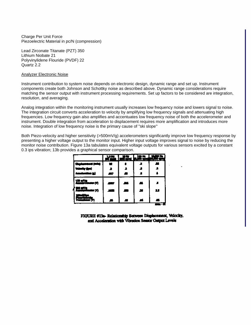
Charge Per Unit Force Piezoelectric Material in pc/N (compression) Lead Zirconate Titanate (PZT) 350 Lithium Niobate 21 Polyvinylidene Flouride (PVDF) 22 Quartz 2.2 Analyzer Electronic Noise Instrument contribution to system noise depends on electronic design, dynamic range and set up. Instrument components create both Johnson and Schottky noise as described above. Dynamic range considerations require matching the sensor output with instrument processing requirements. Set up factors to be considered are integration, resolution, and averaging. Analog integration within the monitoring instrument usually increases low frequency noise and lowers signal to noise. The integration circuit converts acceleration to velocity by amplifying low frequency signals and attenuating high frequencies. Low frequency gain also amplifies and accentuates low frequency noise of both the accelerometer and instrument. Double integration from acceleration to displacement requires more amplification and introduces more noise. Integration of low frequency noise is the primary cause of "ski slope". Both Piezo-velocity and higher sensitivity (>500mV/g) accelerometers significantly improve low frequency response by presenting a higher voltage output to the monitor input. Higher input voltage improves signal to noise by reducing the monitor noise contribution. Figure 13a tabulates equivalent voltage outputs for various sensors excited by a constant 0.3 ips vibration; 13b provides a graphical sensor comparison.

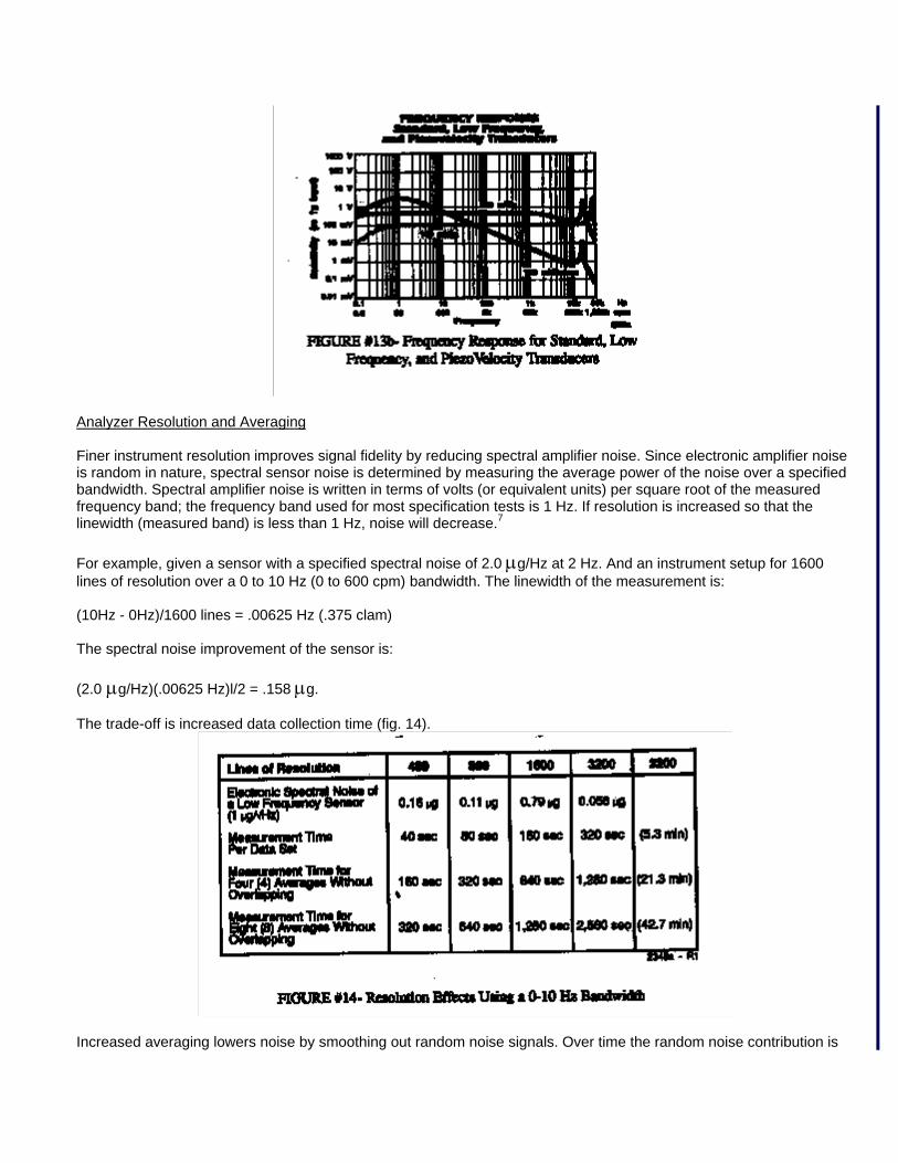
Analyzer Resolution and Averaging Finer instrument resolution improves signal fidelity by reducing spectral amplifier noise. Since electronic amplifier noise is random in nature, spectral sensor noise is determined by measuring the average power of the noise over a specified bandwidth. Spectral amplifier noise is written in terms of volts (or equivalent units) per square root of the measured frequency band; the frequency band used for most specification tests is 1 Hz. If resolution is increased so that the linewidth (measured band) is less than 1 Hz, noise will decrease.7 For example, given a sensor with a specified spectral noise of 2.0 μg/Hz at 2 Hz. And an instrument setup for 1600 lines of resolution over a 0 to 10 Hz (0 to 600 cpm) bandwidth. The linewidth of the measurement is: (10Hz - 0Hz)/1600 lines = .00625 Hz (.375 clam) The spectral noise improvement of the sensor is: (2.0 μg/Hz)(.00625 Hz)l/2 = .158 μg. The trade-off is increased data collection time (fig. 14).

Increased averaging lowers noise by smoothing out random noise signals. Over time the random noise contribution is

reduced and periodic signals strengthened. Like resolution increases, the down side of increased avenging is longer data collection time - as stated patience is a virtue! Calculation of System Noise8 The minimum electronic signal to noise ratio can be easily evaluated if the electronic noise of the sensor and analyzer are known. Since acceleration amplitudes decrease with frequency and the noise increases, the combined noise should be determined at the lowest frequency of interest - it only gets better as the frequency increases! Given that the power spectral noise is measured over a 1 Hz line width and evaluated at the minimum frequency of interest (fmin), the signal to noise ratio (S/N) is:

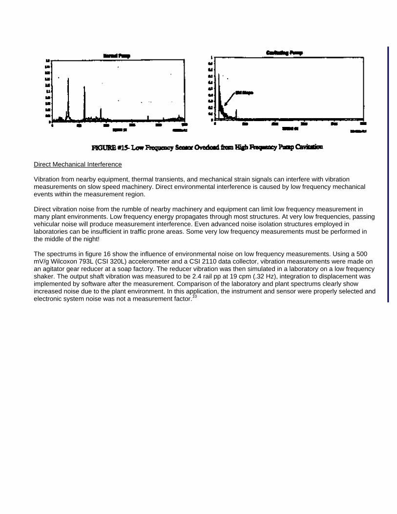
S/N (min) = S / {[(NS)2 + (NA/SV) 2]Δf} 1/2 Where: S = Lowest signal amplitude in EU (Engineering Units - g, m/s2, ips, μm etc) NS = Spectral noise of the sensor in EU/Hz1/2 at fmin NA = Spectral noise of the analyzer in V/Hz1/2 at fmin SV = Sensitivity of the sensor in V/EU Δf = Analyzer resolution in Hz IV. Environmental Interference: Mechanical and Electromagnetic Environmental interference can be caused by any external signal that directly or indirectly interferes with the measurement. Environmental signals can corrupt vibration data and produce false readings. The false readings may be due to direct interference at the frequency of interest or distortion caused by high frequency noise. Interference sources can be caused by electrical or mechanical signals originating from the machine under test, nearby machinery, or the plant structure and environment. Because of the low levels of acceleration at slow speeds, low frequency measurements are very susceptible-to environmental interference. Indirect Mechanical Interference Indirect mechanical interference originates at high frequency and interacts with the measurement system to produce low frequency interference. Common examples include pump cavitation, steam leaks on paper machine dryer cans, compressed air leaks, and gear mesh frequencies. These sources produce high amplitude, high frequency vibration noise (HFVN) and can overload the sensor amplifier to produce low frequency distortion. This type of interference is a form of intermodulation distortion commonly referred to as "washover" distortion; it usually appears as an exaggerated "ski slope".9 Pump cavitation produces HFVN due to the collapse of cavitation bubbles. The spectrums in figure 15 show measurements from identical pumps using a 500 mV/g low frequency accelerometer. The first plot displays expected readings from the normal pump; the second shows ski slope due to pump cavitation and washover distortion. Although cavitation overload can mask low frequency signals, it is a reliable sign of pump wear and can be added to the diagnostic toolbox. Gas leaks are another common source of HFVN. Paper machines contain steam heated dryer cans fitted with high pressure seals. When a seal leak develops, steam exhaust produces very high amplitude noise. Similar to cavitation, the "hiss" overloads the accelerometer amplifier to produce low frequency distortion. Again, this represents a real problem with the machine that must be repaired. Low frequency accelerometers are generally more susceptible to HFVN and washover distortion than general purpose accelerometers. This is due to their lower resonance frequency and higher sensitivity. Piezo-velocity transducers, where applicable, eliminate washover distortion by attenuating HFVN.

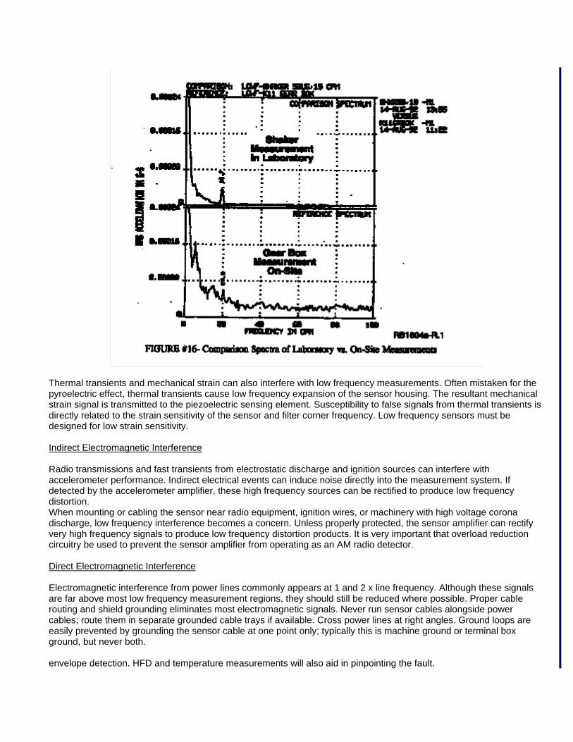
Direct Mechanical Interference Vibration from nearby equipment, thermal transients, and mechanical strain signals can interfere with vibration measurements on slow speed machinery. Direct environmental interference is caused by low frequency mechanical events within the measurement region. Direct vibration noise from the rumble of nearby machinery and equipment can limit low frequency measurement in many plant environments. Low frequency energy propagates through most structures. At very low frequencies, passing vehicular noise will produce measurement interference. Even advanced noise isolation structures employed in laboratories can be insufficient in traffic prone areas. Some very low frequency measurements must be performed in the middle of the night! The spectrums in figure 16 show the influence of environmental noise on low frequency measurements. Using a 500 mV/g Wilcoxon 793L (CSI 320L) accelerometer and a CSI 2110 data collector, vibration measurements were made on an agitator gear reducer at a soap factory. The reducer vibration was then simulated in a laboratory on a low frequency shaker. The output shaft vibration was measured to be 2.4 rail pp at 19 cpm (.32 Hz), integration to displacement was implemented by software after the measurement. Comparison of the laboratory and plant spectrums clearly show increased noise due to the plant environment. In this application, the instrument and sensor were properly selected and electronic system noise was not a measurement factor.10

Thermal transients and mechanical strain can also interfere with low frequency measurements. Often mistaken for the pyroelectric effect, thermal transients cause low frequency expansion of the sensor housing. The resultant mechanical strain signal is transmitted to the piezoelectric sensing element. Susceptibility to false signals from thermal transients is directly related to the strain sensitivity of the sensor and filter corner frequency. Low frequency sensors must be designed for low strain sensitivity. Indirect Electromagnetic Interference Radio transmissions and fast transients from electrostatic discharge and ignition sources can interfere with accelerometer performance. Indirect electrical events can induce noise directly into the measurement system. If detected by the accelerometer amplifier, these high frequency sources can be rectified to produce low frequency distortion. When mounting or cabling the sensor near radio equipment, ignition wires, or machinery with high voltage corona discharge, low frequency interference becomes a concern. Unless properly protected, the sensor amplifier can rectify very high frequency signals to produce low frequency distortion products. It is very important that overload reduction circuitry be used to prevent the sensor amplifier from operating as an AM radio detector. Direct Electromagnetic Interference Electromagnetic interference from power lines commonly appears at 1 and 2 x line frequency. Although these signals are far above most low frequency measurement regions, they should still be reduced where possible. Proper cable routing and shield grounding eliminates most electromagnetic signals. Never run sensor cables alongside power cables; route them in separate grounded cable trays if available. Cross power lines at right angles. Ground loops are easily prevented by grounding the sensor cable at one point only; typically this is machine ground or terminal box ground, but never both. envelope detection. HFD and temperature measurements will also aid in pinpointing the fault.

Most Wilcoxon type accelerometers can be used with the CSI 750 preprocessor demodulation adapter. The Model 750 contains a variety of envelope filter ranges for optimizing the carrier frequency band. When measuring low frequency faults the lower ranges are generally used. 13 Turn on and Settling Time Sensor turn on and settling time are factors in many low frequency applications. In both cases changing bias output voltage is interpreted as a very high level low frequency signal. The varying signal will delay auto-ranging and may corrupt the first several data bins of the spectrum producing significant "ski-slope".14 Turn on is the time it takes the bias voltage to power up to its final rest point. Turn on times of low frequency accelerometers vary from 1 to 8 seconds depending on design. Multiplexed powering systems utilize a time delay before data collection to eliminate spectral corruption. Continuous powered applictions are not affected by turn on time. Settling time can be a much greater problem in walkaround applications. Settling is the time it takes the amplifier bias voltage to recover from shock or thermal overload. Low frequency accelerometer recovery may vary from 2 seconds to 5 minutes! The problem is most evident when using magnets at low frequency. Sensors with overload protection circuitry recover from mounting shock much faster than unprotected sensors. Due to the high sensitivity of low frequency sensors, unprotected amplifiers are also at risk of permanent damage from shock overload. The Wilcoxon 799 accelerometer was designed specifically for low frequency walkaround applications. The 799 contains very sharp low pass filter circuitry that cuts off at 72,000 cpm (1200 Hz). This attenuates magnet mounting shock and reduces shock recovery time. It also contains special bias circuitry to dramatically improve turn on time. When using the 799 with the CSI 750 preprocessor select the 500 Hz high pass filter. Mounting Stud mounts are recommended for low frequency measurements. Use of magnets and probe tips allow the sensor to move at low frequency and disturb the measurement. Handheld measurements can be disturbed by movement of the operators hand (the coffee factor) and cable motion. Stud mounts firmly attach the sensor to the structure and ensure that only vibrations transmitted through the machine surface are measured. Handheld and magnet mounts also exhibit lower mounting resonances and may be more susceptible to HFVN distortion. VI. LOW FREQUENCY APPLICATIONS Rolling Element Bearings Rolling element bearings are often used on very slow speed machinery such as paper machine rollers, agitators and stone crushing equipment. Turning speeds on some machines may be 12 cpm (0.2 Hz) or lower. Generally fault signals are at higher frequencies and well within the measurement capabilities of most systems. However the vibration amplitudes may be buried in noise and must be measured using the envelope demodulation techniques described. Since rolling element bearing faults are not harmonically related to the running speed, time synchronous averaging techniques are not very helpful. Negative averaging may be used to eliminate the synchronous information, but noise will remain. Gear Subharmonics Gear monitoring is generally considered a high frequency application. However, recent studies of spectral information below gear mesh frequency has shown a strong correlation between gear mesh subharmonics and gear tooth faults and wear. Low frequency gear mesh subharmonics, like roller bearing fault frequencies, are not natural vibrations - they are only present when there exists a flaw or developing fault. Subharmonic mesh vibrations occur at the tooth repeat frequency as faulty gear and pinion teeth contact each other.

Tooth repeat frequencies (fTR) can be calculated using the following equation: fTR= (fGear)(NA)/(TPinion) = (fPinion)(NA)/(TGear)

Where: fGear (fpinion) = gear speed (pinion speed) TGear (Tpinion) = number of gear teeth (pinion teeth) NA = number of unique assembly phases The number of unique assembly phases (NA) is equal to the greatest common divisor (GCD) of the number of teeth in both gears in the set. This can be found by calculating the product of the prime factors common to the number of teeth on each gear in the mesh. 15 For example: Given a pinion with 18 teeth, the number 18 is the product of prime numbers 3 x 3 x 2. And given a mating gear with 30 teeth, the number 30 is the product of 5 x 3 x 2. The prime numbers shared between the pinion and the gear are 2 and 3; the product of shared prime numbers (NA) is 6. Primes of 18 Teeth = 3 x 3 x 2 Primes of 30 Teeth = 5 x 3 x 2 Product of Primes NA = 3 x 2 = 6 If on a reducing gear the input drive speed was 900 cpm (15 Hz), the gear mesh equals 162,000 cpm (270 Hz). The tooth repeat frequency in this example is:

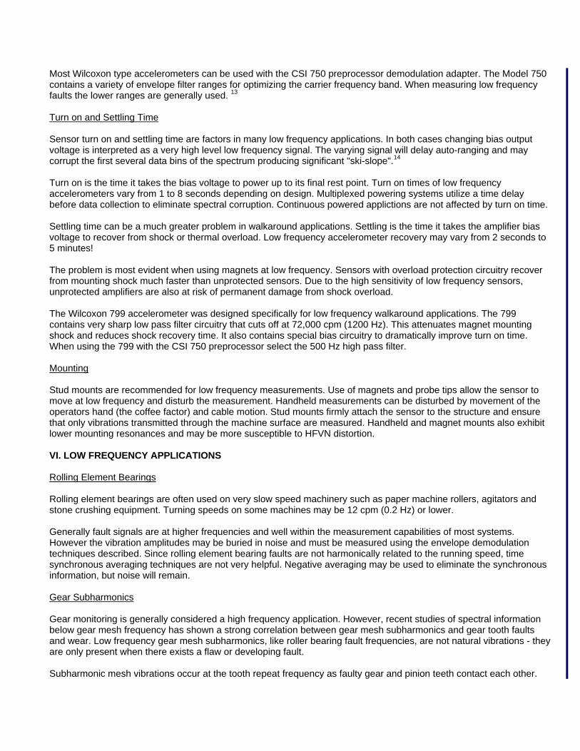
(270 Hz)(6)/(30)(18) - 3 Hz (180 cpm) On more complex gears the Euclidean Algorithm can be used to more efficiently calculate the number of unique assembly phases.16 The tooth repeat frequency for a true hunting tooth gear set, (NA = 1), is the pinion speed divided by the number of gearteeth (or vis versa, fGear/TPinion). Figure 17 shows hunting tooth fault harmonics on a compressor gear set. The motor (gear) drive speed was 29.75 Hz (1785 cpm); the pinion had 30 teeth. Since this was a true hunting tooth gear set, fTR = .99 Hz (59.4 cpm). The fault was caused by indentations made on individual gear and pinion teeth to mark phase of assembly during a rebuild. Interestingly, the hunting tooth harmonics were modulated by a very low frequency (.075 Hz, 4.5 cpm) compressor surge pulsation

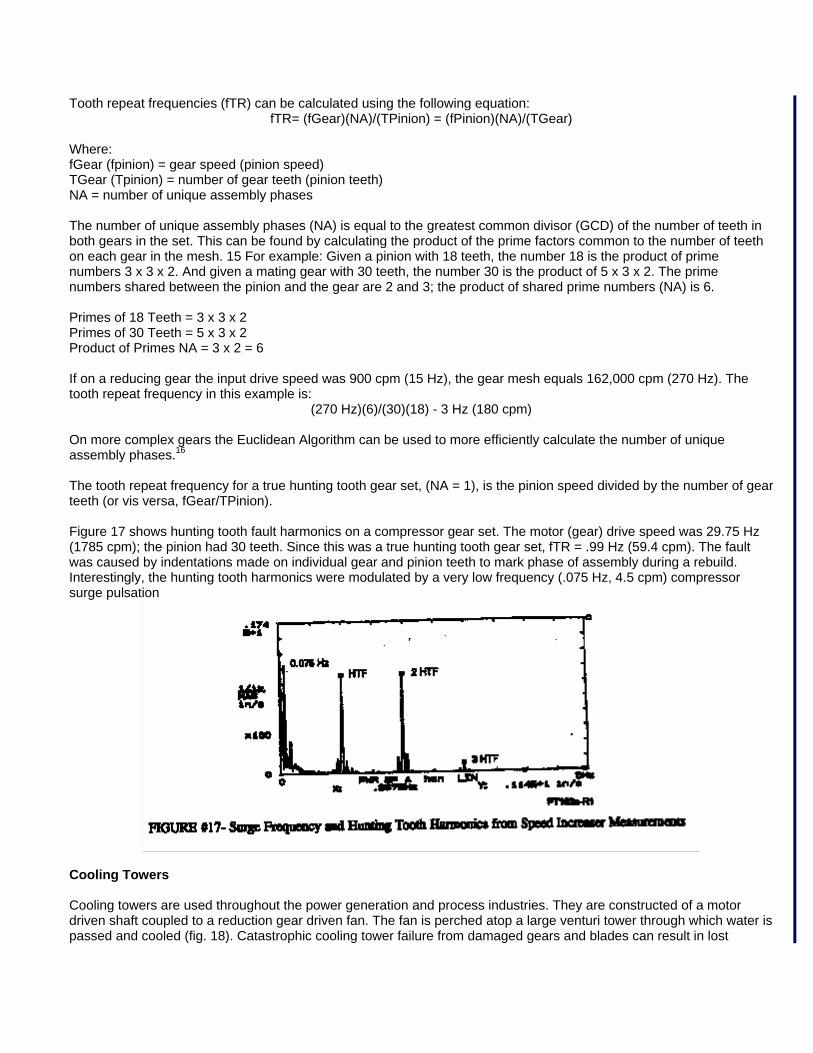
Cooling Towers Cooling towers are used throughout the power generation and process industries. They are constructed of a motor driven shaft coupled to a reduction gear driven fan. The fan is perched atop a large venturi tower through which water is passed and cooled (fig. 18). Catastrophic cooling tower failure from damaged gears and blades can result in lost

production and high repair costs.

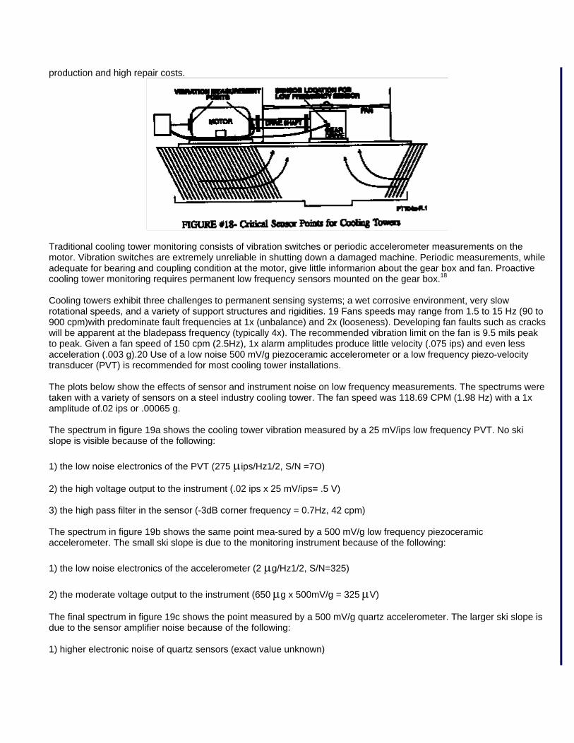
Traditional cooling tower monitoring consists of vibration switches or periodic accelerometer measurements on the motor. Vibration switches are extremely unreliable in shutting down a damaged machine. Periodic measurements, while adequate for bearing and coupling condition at the motor, give little informarion about the gear box and fan. Proactive cooling tower monitoring requires permanent low frequency sensors mounted on the gear box.18 Cooling towers exhibit three challenges to permanent sensing systems; a wet corrosive environment, very slow rotational speeds, and a variety of support structures and rigidities. 19 Fans speeds may range from 1.5 to 15 Hz (90 to 900 cpm)with predominate fault frequencies at 1x (unbalance) and 2x (looseness). Developing fan faults such as cracks will be apparent at the bladepass frequency (typically 4x). The recommended vibration limit on the fan is 9.5 mils peak to peak. Given a fan speed of 150 cpm (2.5Hz), 1x alarm amplitudes produce little velocity (.075 ips) and even less acceleration (.003 g).20 Use of a low noise 500 mV/g piezoceramic accelerometer or a low frequency piezo-velocity transducer (PVT) is recommended for most cooling tower installations. The plots below show the effects of sensor and instrument noise on low frequency measurements. The spectrums were taken with a variety of sensors on a steel industry cooling tower. The fan speed was 118.69 CPM (1.98 Hz) with a 1x amplitude of.02 ips or .00065 g. The spectrum in figure 19a shows the cooling tower vibration measured by a 25 mV/ips low frequency PVT. No ski slope is visible because of the following: 1) the low noise electronics of the PVT (275 μips/Hz1/2, S/N =7O) 2) the high voltage output to the instrument (.02 ips x 25 mV/ips= .5 V) 3) the high pass filter in the sensor (-3dB corner frequency = 0.7Hz, 42 cpm) The spectrum in figure 19b shows the same point mea-sured by a 500 mV/g low frequency piezoceramic accelerometer. The small ski slope is due to the monitoring instrument because of the following: 1) the low noise electronics of the accelerometer (2 μg/Hz1/2, S/N=325) 2) the moderate voltage output to the instrument (650 μg x 500mV/g = 325 μV) The final spectrum in figure 19c shows the point measured by a 500 mV/g quartz accelerometer. The larger ski slope is due to the sensor amplifier noise because of the following: 1) higher electronic noise of quartz sensors (exact value unknown)

2) same voltage output to the instrument as in 19b.

CONCLUSION Reliable low frequency measurement requires strict attention to selection and use of vibration equipment. The low acceleration amplitudes on very slow speed machinery are beyond the measurement limits of general instrumentation and techniques. Concerted efforts to improve the signal to noise ratio of the measurement axe required to best utilize data collection time and effort. Specially designed low frequency piezoceramic sensors are recommended in most applications. Piezoceramic transducers provide superior performance over the broad frequency and amplitude ranges required in industrial applications. They employ low noise electronics, provide high outputs to the instrument, and resist environmental effects. Instruments must be chosen with low frequency input capability and ample dynamic range. Proper instrument design and set up lowers system noise and speeds data collection time. Special techniques can be used to further improve data reliability. The measurement environment must also be evaluated to determine its effects on the data. Low frequency applications and techniques are continually being discovered and refined. A great amount of this work is being carried out using envelope demodulation. A systematic approach toward low frequency condition monitoring helps ensure that reliability based maintenance goals are met. 1. Barrett, Richard, "Industrial Vibration Sensor Selection: Piezo-Velocity Transducers (PVT)" Proc. 17th annual meeting, Vibration Institute, June 1993, 135-140. 2. Schloss, Fred, "Accelerometer Overload", Sound and Vibration, January 1989. 3. Druif, Dave "Extremely Low Frequency Measurement Techniques", Test Report, Computational Sys-tems Incorporated, 1992

4. Technology for Energy, "Very Low Frequency Data Collection" TEC Trends, Jan/Feb 1993. 5. Schloss, Fred "Accelerometer Noise", Sound and Vibration, March 1993, pp 22-23. 6. Robinson, James C.; LeVert, Francis E.; Mott, J.E.; "Vibration Data Aquisition of Low speed Machin-ery (-10 rpm) Using a Portable Data Collector and a Low Impedance Accelerometer", P/PM Technology, May/June, 26-30 1992 7. Judd, John E.; Sensor Noise Considerations in Low Frequency Machinery Vibration Measurements", P/ PM Technology, May/June, 32-36 1992 8. Barrett, Richard, "Minimizing Noise in Low Frequency Measurements" Real-time Update, Hewlett-Packard, Summer 1994, pp 7-9. 9. Computational Systems Inc. "Selection of Proper Sensors for Low Frequency Vibration Measure-ments" Noise & Vibration Control Worldwide, Oct 1988, pg 256. 10. Seeber, Steve, "Low Frequency Measurement Techniques" MidAtlantic Infrared Services. 11. Chandler, Jon K., "Overlap Averaging: A Practical Look", Sound and Vibration, May 1991, pp 24 - 29. 12. Shreve, Dennis, "Special Considerations in Making Low Frequency Vibration Measurements." P/PM Technology, April 1993, pp18-19. 13. Computational Systems Inc. "Demodulation: CSI Model 750 Preprocessor Theory and Application" Trend Setter, Spring 1992, pp 2-5. 14. Robinson, James C.; LeVert, Francis E.; Mott, J.E.; "The Acquisition of Vibration Data from Low-Speed Machinery", Sound and Vibration, May 1992, 22-28 15. Berry James E., PE. "Advanced Vibration Analysis Diagnostic & Corrective Techniques", Discussion of Vibration Diagnostic Chart, Piedmont Chapter #14 of Vibration Institute, Technical Associates of Charlotte Inc., May 27, 1993. 16 Foiles, William C, "Gear Frequencies using the Euclidean Algorithm", Vibrations, September 1994, pp 3-5 17. Lind, Gordon; Barrett, Richard M., Jr., "Low Frequency Vibration Measurement on a Compressor Gear Set", PT102, Wilcoxon Research, April 1993 18. Croix, Rick; Suarez, Steve; Crum Coco "Monitoring System for Cooling Tower and Process Cooler Fans" DataSignal Systems Technical Bulletin. 19. Bernhard, D.L. "Cooling Tower Fan Vibration Monitoring" Cooling Tower Institute 1986 Annual Meeting, Houston TX, IRD Mechanalysis, Jan. 1986 20. Murphy, Dan" Cooling Tower Vibration Analysis" The Marley Cooling Tower Co., Maintenance Technology, July 1991, pp 29-33.

All contents copyright © 1998 - 2006, Computational Systems, Inc. All Rights Reserved.

Send comments to: mhm.info@compsys.com

Last Updated 05/08/03

© Emerson, 1996-2005 Legal and Privacy Statements