Ultramicroscopy 184 (2018) 24–38

Contents lists available at ScienceDirect

Ultramicroscopy

journal homepage: www.elsevier.com/locate/ultramic

Improving microstructural quantification in FIB/SEM nanotomography

Joshua A. Taillon

a , 1 , ∗, Christopher Pellegrinelli b , Yi-Lin Huang

b , Eric D. Wachsman

b , Lourdes G. Salamanca-Riba

a , ∗

a University of Maryland, Materials Science and Engineering, College Park, MD 20742, United States b University of Maryland Energy Research Center, Materials Science and Engineering, College Park, MD 20742, United States

a r t i c l e i n f o

Article history:

Received 31 October 2016

Accepted 28 July 2017

Available online 9 August 2017

Keywords:

Focused ion beam

Scanning electron microscopy

3D reconstruction

Microstructure quantification

Triple phase boundaries

Tortuosity

a b s t r a c t

FIB/SEM nanotomography (FIB- nt ) is a powerful technique for the determination and quantification of the

three-dimensional microstructure in subsurface features. Often times, the microstructure of a sample is

the ultimate determiner of the overall performance of a system, and a detailed understanding of its prop-

erties is crucial in advancing the materials engineering of a resulting device. While the FIB- nt technique

has developed significantly in the 15 years since its introduction, advanced nanotomographic analysis is

still far from routine, and a number of challenges remain in data acquisition and post-processing. In this

work, we present a number of techniques to improve the quality of the acquired data, together with easy-

to-implement methods to obtain “advanced” microstructural quantifications. The techniques are applied

to a solid oxide fuel cell cathode of interest to the electrochemistry community, but the methodologies

are easily adaptable to a wide range of material systems. Finally, results from an analyzed sample are

presented as a practical example of how these techniques can be implemented.

© 2017 Elsevier B.V. All rights reserved.

F

t

u

d

p

a

t

1. Introduction

The first successful research implementation of FIB- nt was re-

ported nearly 15 years ago [1] . The technique has become much

more common as the adoption of combined focused ion beam

– scanning electron microscopy (FIB/SEM) systems has increased,

such that commercial vendors now typically advertise and sell

software packages specifically used to acquire 3D data (some com-

mon packages are: Auto Slice and View [2] , Atlas 5 [3] , Mill and

Monitor [4] , and 3D Acquisition Wizard [5] ). Generally, the 3D data

acquisition process proceeds as follows [6] :

1. To acquire a stack of SEM images, the sample is tilted to an

inclined angle, usually the same as the angular offset between

the electron and ion beams.

2. Using the FIB, a large trench is milled around an area of interest

to expose a “data cube” to be acquired, which is then placed at

the coincidence point of the two beams (see Fig. 1 ).

∗ Corresponding authors.

E-mail addresses: joshua.taillon@nist.gov (J.A. Taillon), riba@umd.edu (L.G.

Salamanca-Riba). 1 Present address: Material Measurement Laboratory, National Institute of Stan-

dards and Technology, Gaithersburg, MD, 20899, United States.

p

v

a

a

i

w

s

t

http://dx.doi.org/10.1016/j.ultramic.2017.07.017

0304-3991/© 2017 Elsevier B.V. All rights reserved.

3. Slices of the sample are milled in the z direction, and after each

mill, an image is taken with the electron beam in the xy plane

(at an angle).

a) If desired, chemical and/or structural information can also

be obtained at each slice by collecting X-ray EDS spectrum

images (EDS) or electron backscatter diffraction (EBSD) pat-

terns as well [7,8] .

4. The slice and image process is repeated using automation soft-

ware supplied with the microscope in order to build up a 3D

volume of data.

IB- nt has been successfully used on a broad variety of sample

ypes, meaning the methods presented in this work will be of

se in a wide range of scientific fields. Inkson et al. [1] initially

eveloped the FIB- nt methodology for examining FeAl nanocom-

osites, but it has since been used for 3D chemical analysis of

lloys [9] , microstructural characterization of Li-ion battery elec-

rodes [10] , and pore structure characterization in shale gas sam-

les [11] . FIB- nt has seen extensive use in the microstructural in-

estigation of solid oxide fuel cell cathodes and anodes [12–29] ,

nd in the characterization of many other materials (see Holzer

nd Cantoni [6] for a thorough review). These works feature excit-

ng findings in a range of materials, but the majority are published

ith a focus on samples and applications, rather than on micro-

copic methodology. As such, there are often only scant descrip-

ions of methodology, and a lack of details about specific methods

J.A. Taillon et al. / Ultramicroscopy 184 (2018) 24–38 25

Fig. 1. Schematic of FIB- nt experimental geometry. The sample is positioned at the

intersection of the electron and ion beams for simultaneous imaging and milling. α

is typically in the range of [50–55] °. Figure adapted from Holzer et al. [14] .

a

d

F

f

i

t

p

e

r

v

a

p

m

s

t

a

w

s

v

t

c

d

a

s

W

s

r

t

p

m

w

(

(

e

(

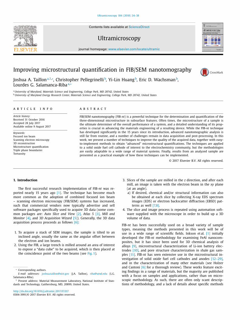
Fig. 2. (a) Photograph of half-cell SOFC stack. A Pt wire (for electrical measure-

ments) is wrapped around the center of the (white) YSZ electrolyte support. The

30 μm cathode layer is visible on the top of the support, and the entire top surface

is coated with an Au contact. (b) Photograph of the SOFC mounted in cross section

after epoxy impregnation, ready for FIB/SEM examination. The sample is mechani-

cally clamped on the sides with three set screws.

m

w

t

a

b

a

c

L

I

a

m

m

n

e

2

2

d

t

p

d

w

o

a

o

p

t

w

m

o

2

a

c

m

nd their implementations. In this work, we introduce and fully

escribe a number of techniques to improve the quality of acquired

IB- nt data. Our specific implementations are also published in a

reely available repository to assist other researchers in the use and

mprovement of the methods presented here [30] .

For the purposes of demonstration, the methods presented in

his work are applied to a solid oxide fuel cell (SOFC) cathode sam-

le. SOFCs are efficient and high-performance electrochemical en-

rgy conversion devices that are fuel flexible and cleaner than cur-

ently used alternatives [31] . On the cathode side of an SOFC de-

ice, the primary goal is the reduction of oxygen, which takes place

t the boundary between the open pore, electrolyte, and cathode

hase, known as the triple phase boundary (TPB). Accordingly, the

orphology and three-dimensional microstructure of the cathode

trongly affect the available sites for oxygen reduction, which in

urn control the cathode polarization and performance.

More specifically, quantifiable microstructural parameters such

s overall porosity, tortuosity ( τ ), and connectivity of the pore net-

ork have specific impacts on the total polarization resistance ob-

erved in the cathode. Other parameters such as surface area and

olume of each phase change the available sites for gas adsorp-

ion within the cathode, while the triple phase boundary length

ontrols overall charge transfer. Many of these parameters can be

irectly quantified using a FIB/SEM. The simplest parameters, such

s porosity, phase surface area and volume, particle size, etc. were

ome of the first to be investigated using this method [14,15,17,18] .

ilson et al. [32] and Gostovic et al. [13] followed with detailed de-

criptions of phase and three-dimensional topological connectivity,

espectively. Many authors have explored the concepts of phase

ortuosity with various approaches, ranging from relatively sim-

le center of mass considerations to more complex finite element

odeling [13,16,20,21,32–34] . A natural extension of these methods

as to examine the three dimensional interface between all phases

the TPB), and to quantify the total triple phase boundary lengths

L TPB ), as well as the fraction of these that were expected to be

lectrochemically active [13,16,22,27,32,33] . In the SOFC literature

and in other fields as well), there is little consensus regarding the

ethods used to measure many of these parameters. Even among

orks from the same research group, the specific techniques used

o calculate L TPB or τ can vary widely (and the implementations

re rarely publicly available), leading to difficulty comparing results

etween reports.

This work describes the specific techniques used to acquire

high resolution image stack from an LSM-YSZ composite SOFC

athode:

SM : ( La 0 . 8 Sr 0 . 2 ) 0 . 95 MnO 3+ δYSZ : (Y 2 O 3 ) 0 . 08 ( Zr O 2 ) 0 . 92

mage acquisition and post-processing strategies are demonstrated

nd discussed, followed by a detailed review of computational

ethods that can be used to calculate various morphological and

icrostructural properties from a three-dimensional dataset. Fi-

ally, implementation of these procedures is demonstrated on an

xample LSM-YSZ cathode sample.

. Experimental procedures

.1. Sample fabrication

An LSM-YSZ composite cathode layer was fabricated using stan-

ard screen printing techniques on a pre-sintered YSZ bulk elec-

rolyte support, yielding an SOFC “half-cell”. For the support, YSZ

owder (TOSOH Corp.) was uniaxially pressed in a 10 mm diameter

ie and sintered at 1450 °C for 6 h. The sintered electrolyte pellet

as then polished to 5 mm thickness. Slurries of composite cath-

de material, made from 50:50 wt.% LSM-YSZ (Fuel Cell Materi-

ls), were screen printed onto the YSZ support, resulting in a cath-

de layer of approximately 30μm. The cathodes (together with the

re-sintered electrolyte) were sintered at 1100 °C for 2 h to remove

he pore-forming material and generate a composite cathode layer

ith porous structure. A gold contact layer (for electrical measure-

ents) was painted onto the surface of the cathode; a photograph

f the cell is shown in Fig. 2 a.

.2. FIB/SEM sample preparation

The quality of a volume reconstruction can be only as high

s each individual image that is acquired during the FIB- nt pro-

ess. Many artifacts common to FIB/SEM can complicate the seg-

entation and reconstruction process, including (but not limited

26 J.A. Taillon et al. / Ultramicroscopy 184 (2018) 24–38

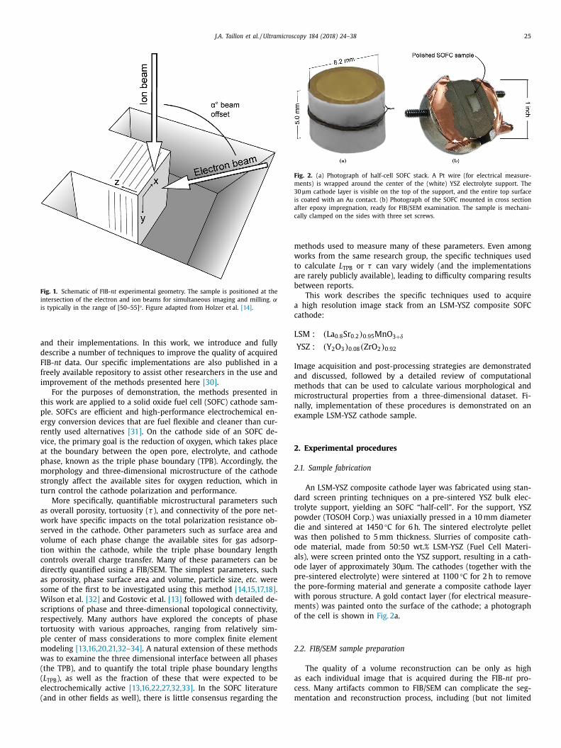
Fig. 3. Examples of common artifacts that can occur during a FIB/SEM nanotomographic acquisition. (a) The “pore-back” effect is the imaging of material that is not on

the current plane of interest, which appears due to electrons escaping from the back of a pore through the open vacuum; (b) curtaining artifacts arise from ion channeling

during the milling process and appear as vertical striations and (c) electron image ( V acc = 5 kV) showing sample charging (bright regions) on a LSM/YSZ cathode that is

typical when imaging poorly conducting materials.

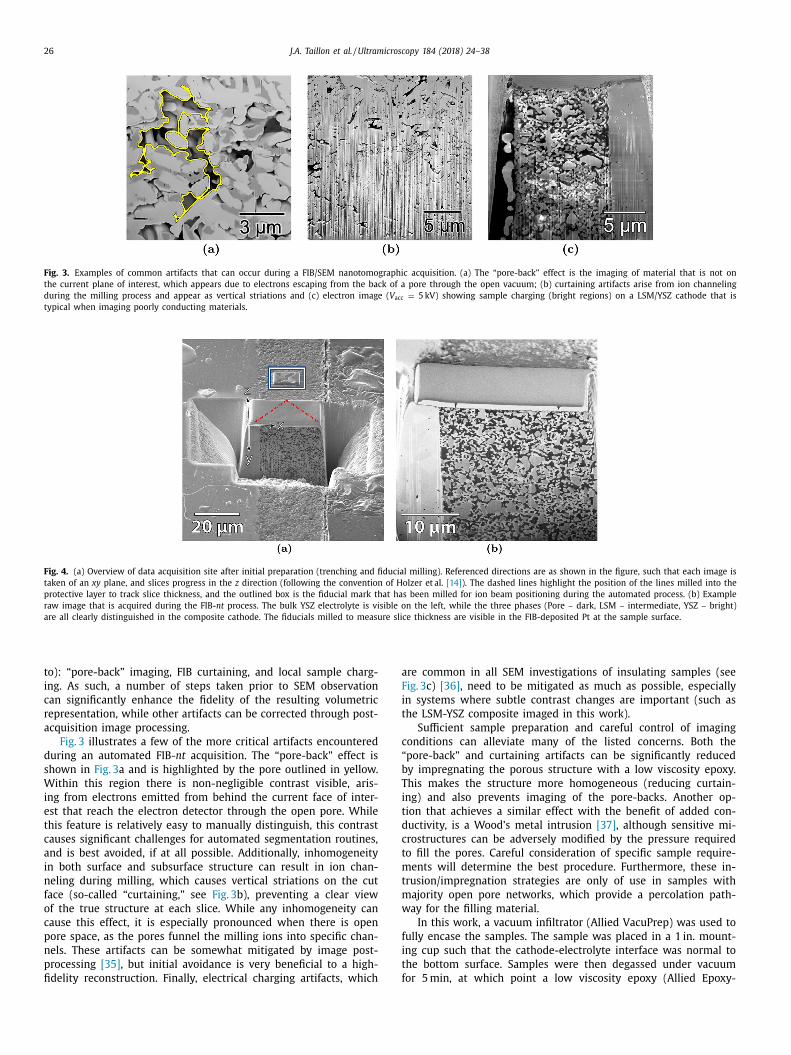
Fig. 4. (a) Overview of data acquisition site after initial preparation (trenching and fiducial milling). Referenced directions are as shown in the figure, such that each image is

taken of an xy plane, and slices progress in the z direction (following the convention of Holzer et al. [14] ). The dashed lines highlight the position of the lines milled into the

protective layer to track slice thickness, and the outlined box is the fiducial mark that has been milled for ion beam positioning during the automated process. (b) Example

raw image that is acquired during the FIB- nt process. The bulk YSZ electrolyte is visible on the left, while the three phases (Pore – dark, LSM – intermediate, YSZ – bright)

are all clearly distinguished in the composite cathode. The fiducials milled to measure slice thickness are visible in the FIB-deposited Pt at the sample surface.

a

F

i

t

c

“

b

T

i

t

d

c

t

m

t

m

w

f

i

t

f

to): “pore-back” imaging, FIB curtaining, and local sample charg-

ing. As such, a number of steps taken prior to SEM observation

can significantly enhance the fidelity of the resulting volumetric

representation, while other artifacts can be corrected through post-

acquisition image processing.

Fig. 3 illustrates a few of the more critical artifacts encountered

during an automated FIB- nt acquisition. The “pore-back” effect is

shown in Fig. 3 a and is highlighted by the pore outlined in yellow.

Within this region there is non-negligible contrast visible, aris-

ing from electrons emitted from behind the current face of inter-

est that reach the electron detector through the open pore. While

this feature is relatively easy to manually distinguish, this contrast

causes significant challenges for automated segmentation routines,

and is best avoided, if at all possible. Additionally, inhomogeneity

in both surface and subsurface structure can result in ion chan-

neling during milling, which causes vertical striations on the cut

face (so-called “curtaining,” see Fig. 3 b), preventing a clear view

of the true structure at each slice. While any inhomogeneity can

cause this effect, it is especially pronounced when there is open

pore space, as the pores funnel the milling ions into specific chan-

nels. These artifacts can be somewhat mitigated by image post-

processing [35] , but initial avoidance is very beneficial to a high-

fidelity reconstruction. Finally, electrical charging artifacts, which

re common in all SEM investigations of insulating samples (see

ig. 3 c) [36] , need to be mitigated as much as possible, especially

n systems where subtle contrast changes are important (such as

he LSM-YSZ composite imaged in this work).

S ufficient sample preparation and careful control of imaging

onditions can alleviate many of the listed concerns. Both the

pore-back” and curtaining artifacts can be significantly reduced

y impregnating the porous structure with a low viscosity epoxy.

his makes the structure more homogeneous (reducing curtain-

ng) and also prevents imaging of the pore-backs. Another op-

ion that achieves a similar effect with the benefit of added con-

uctivity, is a Wood’s metal intrusion [37] , although sensitive mi-

rostructures can be adversely modified by the pressure required

o fill the pores. Careful consideration of specific sample require-

ents will determine the best procedure. Furthermore, these in-

rusion/impregnation strategies are only of use in samples with

ajority open pore networks, which provide a percolation path-

ay for the filling material.

In this work, a vacuum infiltrator (Allied VacuPrep) was used to

ully encase the samples. The sample was placed in a 1 in. mount-

ng cup such that the cathode-electrolyte interface was normal to

he bottom surface. Samples were then degassed under vacuum

or 5 min, at which point a low viscosity epoxy (Allied Epoxy-

J.A. Taillon et al. / Ultramicroscopy 184 (2018) 24–38 27

S

t

i

1

c

r

t

i

i

i

s

w

w

e

c

m

m

2

w

C

i

G

r

a

t

t

t

o

p

c

i

i

b

“

t

i

c

s

e

a

t

h

s

i

d

r

t

t

l

c

n

i

v

s

w

i

u

v

c

i

T

a

p

f

f

a

fi

r

w

T

t

a

w

w

a

e

I

2

n

d

d

(

2

t

i

s

t

t

u

F

O

s

o

w

r

r

t

e

n

S

r

i

w

q

o

F

s

p

m

i

t

p

[

h

(

et) was flowed slowly over each cup, allowing ample time for

he epoxy to fully permeate the porous structure. The epoxy was

ntroduced using a 1/4 ̋ ID flexible tube, allowing approximately

drip (roughly 0.5 mL) per second. Once the samples were fully

overed with epoxy, they were held under vacuum for 1 min and

eturned to atmospheric pressure, at which point they were left

o cure overnight. Once cured, the samples were planarized us-

ng a low grit SiC abrasive paper (LECO). An automated polish-

ng machine (LECO GPX-200) was used to grind the sample us-

ng 320 −1200 grit papers, and then polished with a 3 μm diamond

uspension. To prevent charging, a thin layer (few nm) of carbon

as sputtered (Balzers) onto the polished surface, and the sample

as mounted with conductive graphite paint and Cu tape onto an

poxy mount SEM holder (Ted Pella, Inc.) (see Fig. 2 b). Mechani-

al clamping of the sample is preferred over conductive adhesive

ounting to maximize long-term acquisition stability and mini-

ize physical specimen drift.

.3. FIB/SEM observation

In this work, images for the three-dimensional reconstructions

ere obtained using an FEI Helios 650 dual beam FIB/SEM, at the

enter for Nanoscale Science and Technology (CNST) user facil-

ty at the National Institute for Standards and Technology (NIST,

aithersburg, MD). Once an area of interest is located, the sur-

ounding area should be prepared to maximize the imaging signal

nd structural fidelity. First, a layer of protective Pt (or another ma-

erial) is deposited on the sample surface using the ion beam. Next,

wo angled lines are milled into the deposited platinum, such that

he thickness of each slice can be verified after acquisition

2 [38] ,

n top of which a thick layer of protective carbon is similarly de-

osited. Different deposition materials are used to provide visual

ontrast between the layers, assisting the fiducial pattern track-

ng. Slightly above the area of interest, a fiducial pad (of carbon)

s deposited, and a mark milled into it as a reference for the ion

eam during the automated tomography process. Finally, a large

C-trench” is milled using the highest current to reveal the face of

he desired data cube (see Fig. 4 a).

Oftentimes in a 3D reconstruction, one is interested in segment-

ng two (or more) materials that are very similar in nature. Be-

ause of this, careful consideration of imaging parameters is neces-

ary in order to optimize the contrast between the phases of inter-

st, requiring the balancing of electron yield, interaction volume,

nd sample charging. While the specific settings will need to be

ailored to various material systems, their discussion is included

ere in order to provide insight into the important practical con-

iderations for FIB- nt data acquisition. In the composite cathode

nvestigated in this work, the LSM and YSZ phases are often very

ifficult to distinguish owing to the similarity between and poor

oom temperature conductivity of the materials. Previous work on

his system has revealed sufficient contrast can be extracted from

hese materials using low energy-loss backscattered electrons, col-

ected using an energy filtered backscatter detector [33] . While this

onfiguration was not available on the present tool, adequate (if

ot quite ideal) conditions were found using secondary electron

maging. The primary beam was low-energy, with an accelerating

oltage ( V acc ) of 750 V, and was operated in the magnetic immer-

ion mode. Detection utilized the “through the lens” detector (TLD)

ith a 600 V collection grid bias.

In addition to improving contrast between phases, the low V acc

mproves spatial resolution and reduces the total interaction vol-

me, enhancing the contrast within the epoxy-filled pores and pro-

iding sharper contrast at material edges. To prevent buildup of

2 See the FIB-SEM/fibtracking module of [30] .

g

h

t

harge within the specimen, images were taken using full frame

ntegration of 16 images with a short (100 ns) dwell time per pixel.

o improve the reliability of later quantifications, the field of view

nd resolution of the electron images were selected to result in ap-

roximately isometric voxel sizes (in this sample, ∼ 20 nm). Auto-

ocus and auto-contrast/brightness routines were performed be-

ore every image, resulting in raw images as shown in Fig. 4 b. The

ssignment of particular intensity levels to each phase was con-

rmed prior to the full data acquisition using energy dispersive X-

ay spectroscopy (EDS) scans (Oxford Instruments).

Once the site preparations were completed, the FIB- nt process

as begun using the Auto Slice and View software (FEI Company).

he prepared site was selected as the area of interest and the slice

hickness was nominally set to 20 nm. Through post-acquisition

nalysis of the thickness tracking fiducials, the true slice thickness

as determined to be 20.0 ± 0.3 nm after approximately 40 slices

ere completed. Because earlier slices varied more in thickness

s the beam approached the sample volume, slices taken prior to

quilibration of the slice thickness were omitted from the analysis.

n a typical acquisition, each slice required a total of approximately

.5 min for milling and imaging. In the static geometry used here,

o stage motion is necessary during the FIB- nt collection. For the

ataset presented in this work, 605 usable slices were acquired

uring an approximately 28 h acquisition, yielding a total volume

after cropping) with x, y, z dimensions of (26.4, 19.9, 12.1) μm.

.4. Data pre-processing

In addition to the methods used to acquire the image data,

he processing steps that are taken can greatly affect the qual-

ty and fidelity of the resulting reconstruction. These processing

teps are taken prior to image segmentation in order to facilitate

he image labeling process and minimize the number of errors in

he resulting output. In this work, these steps were implemented

sing a variety of software, including Avizo Fire (FEI Company),

iji (open-source) [39] , and Python libraries such as NumPy [40] ,

penCV [41] , and scikit-image (open-source) [42] . Where pos-

ible, other open-source libraries with similar functionality are rec-

mmended, although may not be specifically implemented in this

ork.

Collected images first require a shearing correction (in the y di-

ection) to account for anisotropic voxel sizes in the x and y di-

ections. This anisotropy is due to the foreshortening caused by

he 52 ° angle of electron beam illumination. Additionally, although

ach image is acquired relative to a predefined fiducial marker, fi-

al alignment using a least-squares optimization (using the ‘Align

lices’ module in Avizo Fire , or the ‘StackReg’ plugin in Fiji [43] ) will

emove any residual artifacts from errant drift correction. Follow-

ng alignment, the volume is then cropped to the area of interest

ithin the acquired data.

Additionally, an intensity gradient is often observed on the ac-

uired slices, due to the shadowing (lower detection efficiency)

f electrons originating from the bottom of the sample face (see

ig. 5 a). The shadowing artifact derives from the geometry of the

ystem, and is a common issue in FIB- nt acquisitions that can com-

licate analysis [23] . Previous researchers have attempted to re-

ove this artifact by changing the sample geometry. One method

n particular, the block lift-out technique, has been demonstrated

o be very successful, but requires a great deal of time (6 h to pre-

are a 20 × 20 × 20 μm

3 volume prior to any data acquisition)

6,44] . The shadowing in Fig. 5 a causes an overlap within the global

istogram between the brightest (YSZ) and moderate-intensity

LSM) phases. Bright pixels towards the bottom will be incorrectly

rouped with the moderate pixels towards the top, which greatly

inders the segmentation procedure. While the darker portions at

he bottom of the images could be cropped to remove the artifact

28 J.A. Taillon et al. / Ultramicroscopy 184 (2018) 24–38

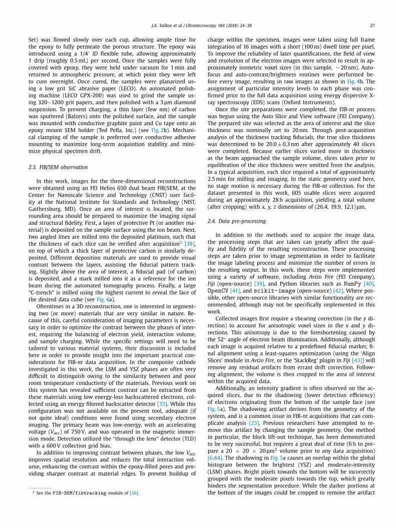
Fig. 5. Example of an acquired image (a) before and (c) after FIB trench shading normalization. (b) Shows the “reslicing” of the sample volume that enables the normalization.

(d) Histogram and kernel density estimate for each image. After shading correction, the image is no longer undersaturated, and there is greatly improved contrast between

the three phases, evidenced by the emergence of clearer intensity peaks (although still overlapping). In particular, much of the illumination in the [ 50 − 100 ] range (top,

red) has been corrected into the pore and LSM peaks at 20 and 160, respectively (bottom, green). All images are displayed on the same brightness/contrast scale. (For

interpretation of the references to colour in this figure legend, the reader is referred to the web version of this article.)

2

i

t

t

t

t

p

[

a

v

a

l

t

r

s

t

t

(

t

v

o

t

u

(at the expense of the total reconstructed volume), a correction

mechanism is preferred to quickly enable full use of the acquired

data.

A unique method to correct the intensity gradient observed

in the images is presented in Fig. 5 . The technique relies on the

fact that the intensity gradient is relatively constant on successive

slices in the z -direction and is only present in the y -direction. By

“reslicing” the image data onto an orthogonal set of xz -planes, the

gradient can be easily corrected. The original ( xy ) images will have

a gradient, but xz images will have uniform illumination on each

slice and get progressively darker as the stack progresses in the y -

direction ( Fig. 5 b). Each successive xz image can be normalized to

the first by matching the first and second order statistics of the

images’ probability distribution functions [45] . This normalization

along the y dimension effectively removes the intensity gradient

once the data is resliced to its original orientation (compare Fig. 5 a

and c). While surprisingly simple, this method greatly improves

the segmentation results by reducing the amount of pixel-intensity

overlap between adjacent phases ( Fig. 5 d) [30] .

Finally, after all corrections are made, the images are filtered

using a two-dimensional, edge-preserving non-local means filter

implemented within Avizo Fire [46] . This filter is extremely ef-

fective at removing the noise present in FIB/SEM images while

retaining the fidelity of edges between particles. Various open-

source implementations of this algorithm are additionally available

[47,48] .

m

.5. Image segmentation

As the number of phases present in a sample is increased, so

s the complexity of an automated segmentation strategy. For a

hree-component system such as that in the present study, simple

hresholding does not suffice to accurately label the particles con-

ained within the volume. Manual intervention should also be kept

o a minimum, for the sake of reproducibility as well as through-

ut. In this work, a marker-based watershed algorithm was used

49] , implemented within Avizo Fire . The markers were set by using

conservative thresholding, such that only a fraction of the total

olume is assigned to a phase. Each catchment basin is then filled

ccording to the local gradient of illumination. This technique al-

ows for a mostly automated process, requiring limited manual in-

ervention to ensure that particularly challenging particles are cor-

ectly segmented. Final processing of the dataset involves restricted

moothing of the labels to reduce unphysically sharp corners, and

he removal of small “island” particles, which may be formed by

he presence of spurious single or few voxel labels. This segmented

binarized) dataset then formed the basis of the following quanti-

ative analysis.

It should be noted that there is significant opportunity for ad-

ancement in this area. Current commercial solutions typically rely

n simple thresholding (with Avizo Fire’s watershed implementa-

ion a notable exception) to label images into a segmented vol-

me, often requiring extensive human interaction. A number of

ore advanced segmentation algorithms utilizing modern research

J.A. Taillon et al. / Ultramicroscopy 184 (2018) 24–38 29

i

s

t

a

a

3

c

S

m

i

h

p

a

d

3

3

b

F

V

n

a

s

u

f

r

b

T

p

a

o

t

e

u

p

η

C

a

d

3

e

m

w

D

S

T

e

v

n

F

d

c

s

p

w

3

c

o

o

t

p

t

c

c

c

v

e

o

t

m

i

3

r

p

m

n

b

r

t

[

t

‘

v

a

f

f

t

p

c

t

t

i

t

g

t

n

t

u

n

t

i

t

b

p

w

t

L

f

t

q

i

L

i

n the machine learning and computer vision fields have been pre-

ented in the literature (see [50–53] ). Application of these methods

o FIB- nt data could greatly facilitate the reconstruction process,

nd would improve one of the most difficult and time-consuming

spects of the technique.

. Computational procedures

Once a segmented volume has been acquired, various mi-

rostructural parameters can be measured and calculated. In

OFCs, these values can then be directly related to cell perfor-

ance. A number of these parameters have been well described

n prior works [13,14,32] , and as such will only be briefly reviewed

ere. A more detailed discussion is provided for the calculation of

hase connectivity, phase tortuosity ( τ ), and triple phase bound-

ry density ( ρTPB ), as novel methods for these calculations were

eveloped specifically during this work.

.1. Volume quantifications

.1.1. Phase volume fractions ( η)

The volume and surface area of each phase can be calculated

y generating a surface representation of each phase within Avizo

ire (analogous functionality is available using the Blender [54] or

TK [55] open-source software packages). Such routines create a

etwork of triangles (mesh) to represent a particular phase with

three dimensional surface. Once the meshes are obtained, basic

tatistics for each phase can be calculated, including the total vol-

me and surface area (in Avizo , this is accomplished with the ‘Sur-

ace Area Volume’ module), as well as the surface area to volume

atio ( SA:V ). The volume fraction for each phase can be obtained

y dividing the volume of each phase by the total sample volume.

his method of using a surface mesh is more accurate than a sim-

le counting of voxels (used in prior works [18] ), particularly for

rea calculations. This is because a voxel counting algorithm will

verestimate the total surface area due to the discrete nature of

he rectilinear voxel edges. For SOFC materials, solid fractions for

ach cathode phase ( ηsolid ) can be computed as the fractional vol-

me for each solid phase (LSM and YSZ) relative to the total solid

hase volume:

solid , LSM

=

V LSM

V LSM

+ V YSZ

(1)

omparing these ratios to those of the source materials enables

n analysis of potential mass transfer from one phase to another

uring cell operation.

.1.2. Particle size ( d )

From the surface area and volume measurements, a global av-

rage of particle sizes can be determined through the use of a for-

ula common in the Brunauer, Emmett, and Teller (BET) method,

hich measures powder sizes using gas adsorption techniques:

= 6 × V/S, where D is the average particle diameter and V and

are the total phase volume and surface area, respectively [14,56] .

his method assumes spherical particle geometry, which is gen-

rally an invalid assumption for these types of particles, but pro-

ides a simple means by which to compare the particle size mag-

itude of the various phases, and has been used in numerous prior

IB/SEM reconstruction studies [14,18–20,26,57] . If desired, further

etail regarding the distribution of these parameters can be cal-

ulated as well, provided that individual particles can be suitably

eparated (which is not often the case for a very well percolated

hase like those observed in the SOFC sample investigated in this

ork).

.1.3. Phase distribution

Phase distributions throughout each sample volume can be

omputed by examining profiles of the distribution in each orthog-

nal direction ( x, y , and z ). This is useful for investigating whether

r not any anisotropic ordering is present within the phases. In

his work, the distribution was calculated as the fraction of each

lane that was occupied by each material along the profile direc-

ion. Within Avizo , this is accomplished using the ‘Volume per slice’

alculation available in the ‘Material Statistics’ module, but such a

alculation would be relatively simple to implement in any other

omputing environment ( e.g., Python and NumPy ). In addition to

iewing the phase distribution, the slope obtained by fitting a lin-

ar function to this profile allows for a measure of the magnitude

f the change in η ( ∇η), which can be compared between direc-

ions and samples. Variations in the phase distribution could imply

igration of phases within the volume, and could have significant

mpacts on transport kinetics.

.2. Phase connectivity

The interconnectivity of different phases in a sample is a pa-

ameter that is often critical in determining the bulk transport

roperties and possible kinetic pathways of various reactions that

ay take place within it. A common technique to analyze this con-

ectivity is to “skeletonize” the structure, making use of any num-

er of possible algorithms [58] . The goal of these methods is to

epresent each phase by a graph that is homotopic (representa-

ive), thin (single voxel), and medial (at the center of the phase)

59,60] . In this work, Avizo Fire was used to calculate the skele-

ons (in particular, the ‘Distance Map,’ ‘Distance-Ordered Thinner,’

Trace Lines,’ and ‘Evaluate on Lines’ modules). Using these indi-

idual modules (rather than the supplied “Auto Skeleton” feature)

llowed for careful tailoring of module inputs to obtain a skeleton

ree of “starburst” artifacts, which are often produced using the de-

ault settings, especially in areas with large particles. Similar func-

ionality is available in the ITK [61,62] and CGAL [63,64] libraries.

Using one of these techniques, the skeleton network for each

hase can be calculated, and they each consist of one or more dis-

rete graphs . Each graph in turn is comprised of a series of nodes

hat are connected by edges . A number of useful statistics regarding

he network can be figured, many of which were first introduced

n the SOFC literature by Gostovic et al. [13] . A brief overview of

hese metrics is provided here, and a simple illustration of each is

iven in Fig. 6 for reference. Useful among the quantifiable parame-

ers are the number of edges ( E ) and nodes ( N ) within the skeleton

etwork of each phase, as well as their volumetric density, relative

o total sample volume ( ρE and ρN , respectively). From these val-

es, the degree of each node ( k i ) can be calculated by counting the

umber of edges coinciding at each node: k i = E i /N i . The mean of

hese values ( k ) gives a measure of the amount of self-connectivity

n each phase [13] . Finally, the mean topological length ( L ) defines

he average distance throughout the network that can be traveled

etween branching nodes. Physically, this property can be inter-

reted as a sort of mean free path for particles traversing the net-

ork. L is calculated by summing the lengths of each edge within

he network ( l i ) and dividing by the number of nodes present:

=

1

N

∑

i

l i . (2)

In addition to these metrics from previous works, another use-

ul measurement that can be obtained from the skeleton model is

he degree of percolation for a phase ( p ). This parameter aims to

uantify the fraction of the overall skeleton network length that is

nterconnected (percolated). Each phase network (with total length

and mean topological length L ) consists of a finite number of

ndividual graphs (with lengths L ), and each graph represents a

i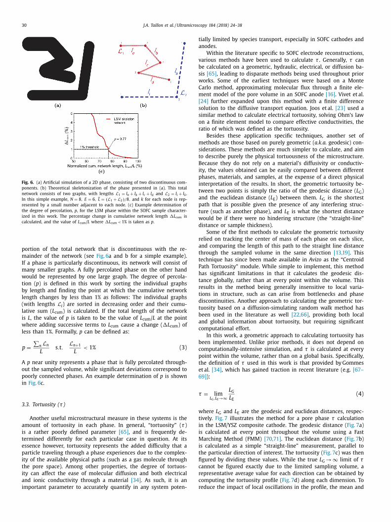

30 J.A. Taillon et al. / Ultramicroscopy 184 (2018) 24–38

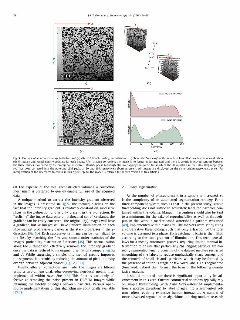
Fig. 6. (a) Artificial simulation of a 2D phase, consisting of two discontinuous com-

ponents. (b) Theoretical skeletonization of the phase presented in (a). This total

network consists of two graphs, with lengths L 1 = l a + l b + l c + l d and L 2 = l i + l ii .

In this simple example, N = 8 , E = 6 , L = ( L 1 + L 2 ) / 8 , and k for each node is rep-

resented by a small number adjacent to each node. (c) Example determination of

the degree of percolation, p , for the LSM phase within the SOFC sample character-

ized in this work. The percentage change in cumulative network length �L cum is

calculated, and the value of L cum / L where �L cum < 1% is taken as p .

t

a

v

b

s

w

C

m

[

s

s

o

r

m

s

t

B

i

p

i

t

a

p

t

w

d

r

a

t

t

P

h

t

r

t

d

t

b

a

c

b

c

p

t

e

6

τ

w

t

i

i

M

i

t

fi

c

r

c

r

portion of the total network that is discontinuous with the re-

mainder of the network (see Fig. 6 a and b for a simple example).

If a phase is particularly discontinuous, its network will consist of

many smaller graphs. A fully percolated phase on the other hand

would be represented by one large graph. The degree of percola-

tion ( p ) is defined in this work by sorting the individual graphs

by length and finding the point at which the cumulative network

length changes by less than 1% as follows: The individual graphs

(with lengths L i ) are sorted in decreasing order and their cumu-

lative sum ( L cum

) is calculated. If the total length of the network

is L , the value of p is taken to be the value of L cum

/ L at the point

where adding successive terms to L cum

cause a change ( �L cum

) of

less than 1%. Formally, p can be defined as:

p =

∑

n L n

L s . t .

L n +1

L < 1% (3)

A p near unity represents a phase that is fully percolated through-

out the sampled volume, while significant deviations correspond to

poorly connected phases. An example determination of p is shown

in Fig. 6 c.

3.3. Tortuosity ( τ )

Another useful microstructural measure in these systems is the

amount of tortuosity in each phase. In general, “tortuosity” ( τ )

is a rather poorly defined parameter [65] , and is frequently de-

termined differently for each particular case in question. At its

essence however, tortuosity represents the added difficulty that a

particle traveling through a phase experiences due to the complex-

ity of the available physical paths (such as a gas molecule through

the pore space). Among other properties, the degree of tortuos-

ity can affect the ease of molecular diffusion and both electrical

and ionic conductivity through a material [34] . As such, it is an

important parameter to accurately quantify in any system poten-

ially limited by species transport, especially in SOFC cathodes and

nodes.

Within the literature specific to SOFC electrode reconstructions,

arious methods have been used to calculate τ . Generally, τ can

e calculated on a geometric, hydraulic, electrical, or diffusion ba-

is [65] , leading to disparate methods being used throughout prior

orks. Some of the earliest techniques were based on a Monte

arlo method, approximating molecular flux through a finite ele-

ent model of the pore volume in an SOFC anode [16] . Vivet et al.

24] further expanded upon this method with a finite difference

olution to the diffusive transport equation. Joos et al. [23] used a

imilar method to calculate electrical tortuosity, solving Ohm’s law

n a finite element model to compare effective conductivities, the

atio of which was defined as the tortuosity.

Besides these application specific techniques, another set of

ethods are those based on purely geometric ( a.k.a. geodesic) con-

iderations. These methods are much simpler to calculate, and aim

o describe purely the physical tortuousness of the microstructure.

ecause they do not rely on a material’s diffusivity or conductiv-

ty, the values obtained can be easily compared between different

hases, materials, and samples, at the expense of a direct physical

nterpretation of the results. In short, the geometric tortuosity be-

ween two points is simply the ratio of the geodesic distance ( L G )

nd the euclidean distance ( L E ) between them. L G is the shortest

ath that is possible given the presence of any interfering struc-

ure (such as another phase), and L E is what the shortest distance

ould be if there were no hindering structure (the “straight-line”

istance or sample thickness).

Some of the first methods to calculate the geometric tortuosity

elied on tracking the center of mass of each phase on each slice,

nd comparing the length of this path to the straight line distance

hrough the sampled volume in the same direction [13,19] . This

echnique has since been made available in Avizo as the “Centroid

ath Tortuosity” module. While simple to implement, this method

as significant limitations in that it calculates the geodesic dis-

ance globally, rather than at every point within the volume. This

esults in the method being generally insensitive to local varia-

ions in structure, such as can arise from bottlenecks and phase

iscontinuities. Another approach to calculating the geometric tor-

uosity based on a diffusion-simulating random walk method has

een used in the literature as well [22,66] , providing both local

nd global information about tortuosity, but requiring significant

omputational effort.

In this work, a geometric approach to calculating tortuosity has

een implemented. Unlike prior methods, it does not depend on

omputationally-intensive simulation, and τ is calculated at every

oint within the volume, rather than on a global basis. Specifically,

he definition of τ used in this work is that provided by Gommes

t al. [34] , which has gained traction in recent literature (e.g. [67–

9] ):

= lim

L G ,L E →∞

L G L E

(4)

here L G and L E are the geodesic and euclidean distances, respec-

ively. Fig. 7 illustrates the method for a pore phase τ calculation

n the LSM/YSZ composite cathode. The geodesic distance ( Fig. 7 a)

s calculated at every point throughout the volume using a Fast

arching Method (FMM) [70,71] . The euclidean distance ( Fig. 7 b)

s calculated as a simple “straight-line” measurement, parallel to

he particular direction of interest. The tortuosity ( Fig. 7 c) was then

gured by dividing these values. While the true L G → ∞ limit of τannot be figured exactly due to the limited sampling volume, a

epresentative average value for each direction can be obtained by

omputing the tortuosity profile ( Fig. 7 d) along each dimension. To

educe the impact of local oscillations in the profile, the mean and

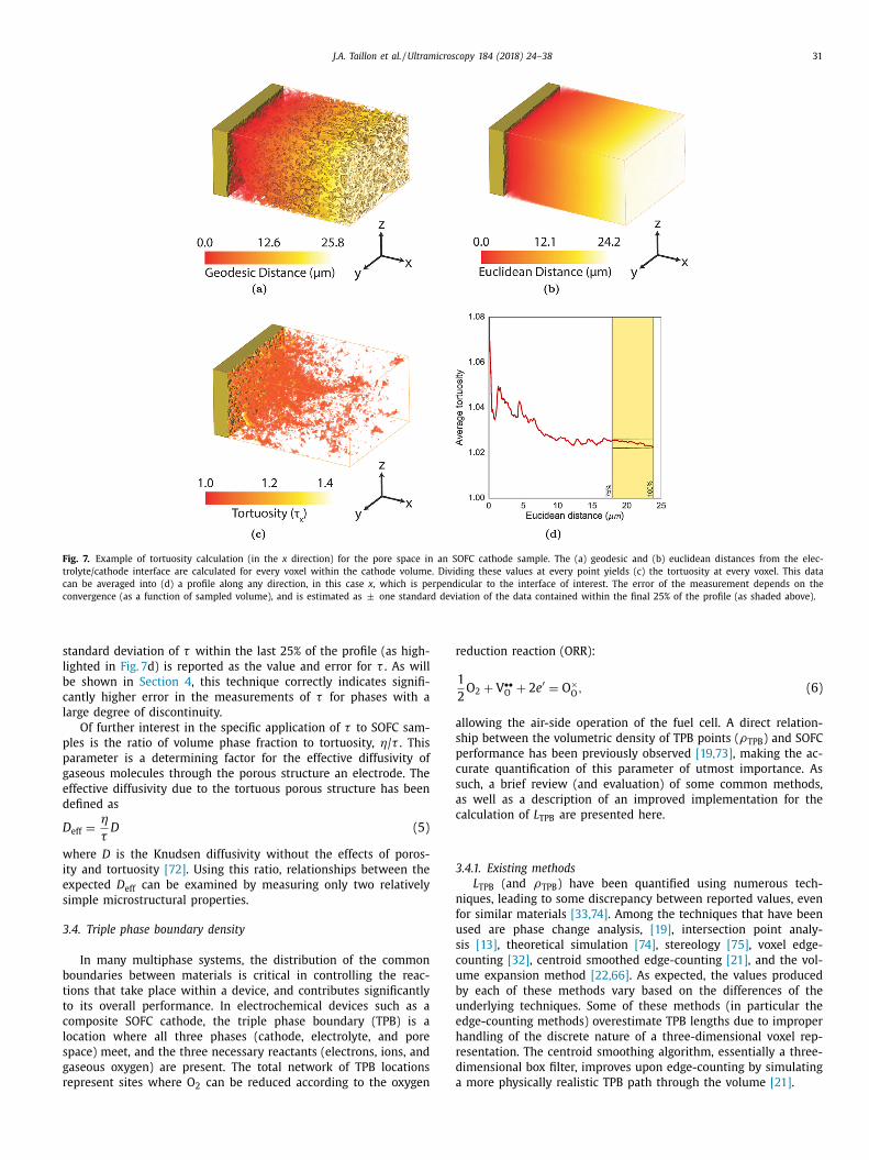
J.A. Taillon et al. / Ultramicroscopy 184 (2018) 24–38 31

Fig. 7. Example of tortuosity calculation (in the x direction) for the pore space in an SOFC cathode sample. The (a) geodesic and (b) euclidean distances from the elec-

trolyte/cathode interface are calculated for every voxel within the cathode volume. Dividing these values at every point yields (c) the tortuosity at every voxel. This data

can be averaged into (d) a profile along any direction, in this case x , which is perpendicular to the interface of interest. The error of the measurement depends on the

convergence (as a function of sampled volume), and is estimated as ± one standard deviation of the data contained within the final 25% of the profile (as shaded above).

s

l

b

c

l

p

p

g

e

d

D

w

i

e

s

3

b

t

t

c

l

s

g

r

r

a

s

p

c

s

a

c

3

n

f

u

s

c

u

b

u

e

h

r

d

a

tandard deviation of τ within the last 25% of the profile (as high-

ighted in Fig. 7 d) is reported as the value and error for τ . As will

e shown in Section 4 , this technique correctly indicates signifi-

antly higher error in the measurements of τ for phases with a

arge degree of discontinuity.

Of further interest in the specific application of τ to SOFC sam-

les is the ratio of volume phase fraction to tortuosity, η/ τ . This

arameter is a determining factor for the effective diffusivity of

aseous molecules through the porous structure an electrode. The

ffective diffusivity due to the tortuous porous structure has been

efined as

eff =

η

τD (5)

here D is the Knudsen diffusivity without the effects of poros-

ty and tortuosity [72] . Using this ratio, relationships between the

xpected D eff can be examined by measuring only two relatively

imple microstructural properties.

.4. Triple phase boundary density

In many multiphase systems, the distribution of the common

oundaries between materials is critical in controlling the reac-

ions that take place within a device, and contributes significantly

o its overall performance. In electrochemical devices such as a

omposite SOFC cathode, the triple phase boundary (TPB) is a

ocation where all three phases (cathode, electrolyte, and pore

pace) meet, and the three necessary reactants (electrons, ions, and

aseous oxygen) are present. The total network of TPB locations

epresent sites where O can be reduced according to the oxygen

2

eduction reaction (ORR):

1

2

O 2 + V

••O + 2 e ′ = O

×O , (6)

llowing the air-side operation of the fuel cell. A direct relation-

hip between the volumetric density of TPB points ( ρTPB ) and SOFC

erformance has been previously observed [19,73] , making the ac-

urate quantification of this parameter of utmost importance. As

uch, a brief review (and evaluation) of some common methods,

s well as a description of an improved implementation for the

alculation of L TPB are presented here.

.4.1. Existing methods

L TPB (and ρTPB ) have been quantified using numerous tech-

iques, leading to some discrepancy between reported values, even

or similar materials [33,74] . Among the techniques that have been

sed are phase change analysis, [19] , intersection point analy-

is [13] , theoretical simulation [74] , stereology [75] , voxel edge-

ounting [32] , centroid smoothed edge-counting [21] , and the vol-

me expansion method [22,66] . As expected, the values produced

y each of these methods vary based on the differences of the

nderlying techniques. Some of these methods (in particular the

dge-counting methods) overestimate TPB lengths due to improper

andling of the discrete nature of a three-dimensional voxel rep-

esentation. The centroid smoothing algorithm, essentially a three-

imensional box filter, improves upon edge-counting by simulating

more physically realistic TPB path through the volume [21] .

32 J.A. Taillon et al. / Ultramicroscopy 184 (2018) 24–38

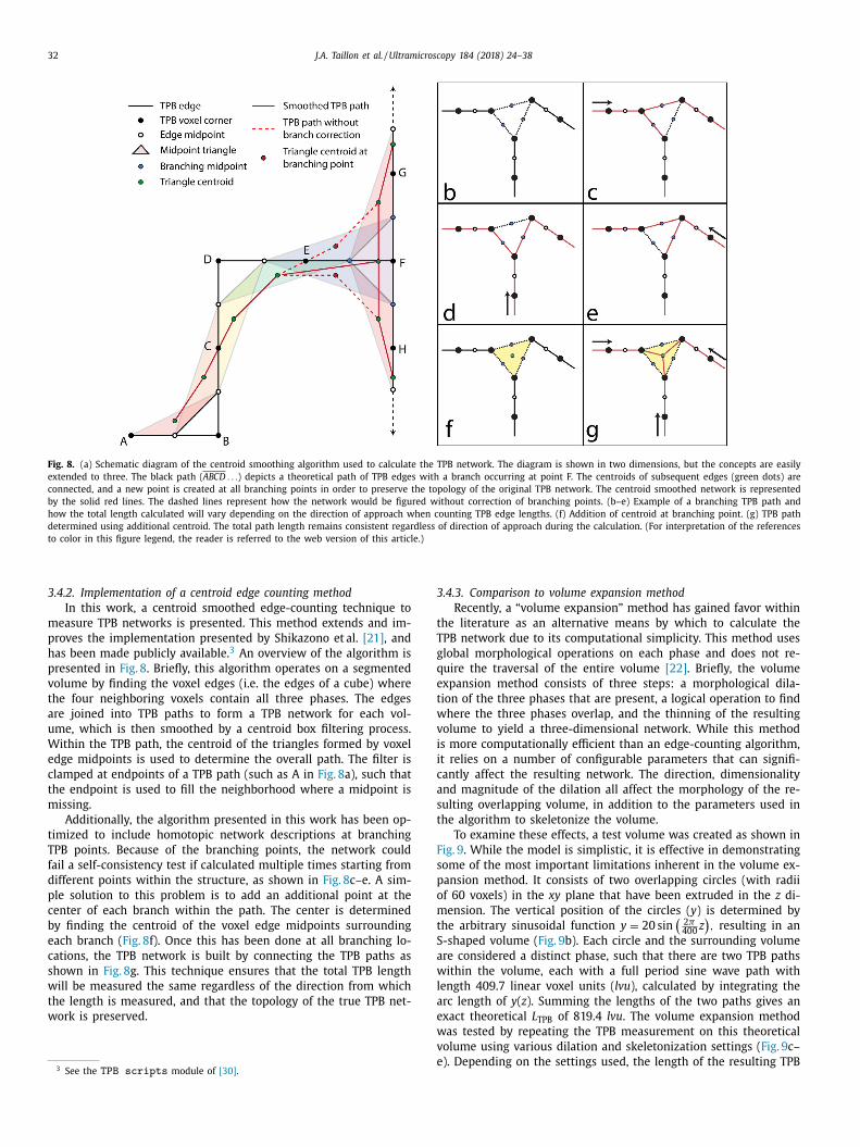
Fig. 8. (a) Schematic diagram of the centroid smoothing algorithm used to calculate the TPB network. The diagram is shown in two dimensions, but the concepts are easily

extended to three. The black path ( ABCD . . . ) depicts a theoretical path of TPB edges with a branch occurring at point F. The centroids of subsequent edges (green dots) are

connected, and a new point is created at all branching points in order to preserve the topology of the original TPB network. The centroid smoothed network is represented

by the solid red lines. The dashed lines represent how the network would be figured without correction of branching points. (b–e) Example of a branching TPB path and

how the total length calculated will vary depending on the direction of approach when counting TPB edge lengths. (f) Addition of centroid at branching point. (g) TPB path

determined using additional centroid. The total path length remains consistent regardless of direction of approach during the calculation. (For interpretation of the references

to color in this figure legend, the reader is referred to the web version of this article.)

3

t

T

g

q

e

t

w

v

i

i

c

a

s

t

F

s

p

o

m

t

S

a

w

l

a

e

3.4.2. Implementation of a centroid edge counting method

In this work, a centroid smoothed edge-counting technique to

measure TPB networks is presented. This method extends and im-

proves the implementation presented by Shikazono et al. [21] , and

has been made publicly available. 3 An overview of the algorithm is

presented in Fig. 8 . Briefly, this algorithm operates on a segmented

volume by finding the voxel edges (i.e. the edges of a cube) where

the four neighboring voxels contain all three phases. The edges

are joined into TPB paths to form a TPB network for each vol-

ume, which is then smoothed by a centroid box filtering process.

Within the TPB path, the centroid of the triangles formed by voxel

edge midpoints is used to determine the overall path. The filter is

clamped at endpoints of a TPB path (such as A in Fig. 8 a), such that

the endpoint is used to fill the neighborhood where a midpoint is

missing.

Additionally, the algorithm presented in this work has been op-

timized to include homotopic network descriptions at branching

TPB points. Because of the branching points, the network could

fail a self-consistency test if calculated multiple times starting from

different points within the structure, as shown in Fig. 8 c–e. A sim-

ple solution to this problem is to add an additional point at the

center of each branch within the path. The center is determined

by finding the centroid of the voxel edge midpoints surrounding

each branch ( Fig. 8 f). Once this has been done at all branching lo-

cations, the TPB network is built by connecting the TPB paths as

shown in Fig. 8 g. This technique ensures that the total TPB length

will be measured the same regardless of the direction from which

the length is measured, and that the topology of the true TPB net-

work is preserved.

3 See the TPB scripts module of [30] .

w

v

e

.4.3. Comparison to volume expansion method

Recently, a “volume expansion” method has gained favor within

he literature as an alternative means by which to calculate the

PB network due to its computational simplicity. This method uses

lobal morphological operations on each phase and does not re-

uire the traversal of the entire volume [22] . Briefly, the volume

xpansion method consists of three steps: a morphological dila-

ion of the three phases that are present, a logical operation to find

here the three phases overlap, and the thinning of the resulting

olume to yield a three-dimensional network. While this method

s more computationally efficient than an edge-counting algorithm,

t relies on a number of configurable parameters that can signifi-

antly affect the resulting network. The direction, dimensionality

nd magnitude of the dilation all affect the morphology of the re-

ulting overlapping volume, in addition to the parameters used in

he algorithm to skeletonize the volume.

To examine these effects, a test volume was created as shown in

ig. 9 . While the model is simplistic, it is effective in demonstrating

ome of the most important limitations inherent in the volume ex-

ansion method. It consists of two overlapping circles (with radii

f 60 voxels) in the xy plane that have been extruded in the z di-

ension. The vertical position of the circles ( y ) is determined by

he arbitrary sinusoidal function y = 20 sin

(2 π400 z

), resulting in an

-shaped volume ( Fig. 9 b). Each circle and the surrounding volume

re considered a distinct phase, such that there are two TPB paths

ithin the volume, each with a full period sine wave path with

ength 409.7 linear voxel units ( lvu ), calculated by integrating the

rc length of y ( z ). Summing the lengths of the two paths gives an

xact theoretical L TPB of 819.4 lvu . The volume expansion method

as tested by repeating the TPB measurement on this theoretical

olume using various dilation and skeletonization settings ( Fig. 9 c–

). Depending on the settings used, the length of the resulting TPB

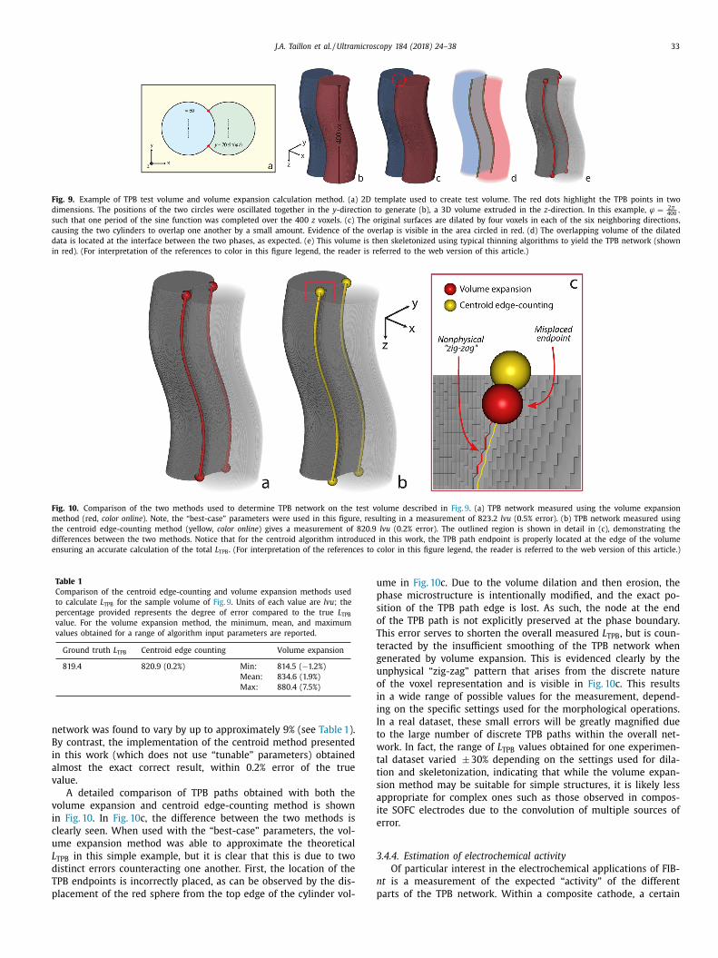
J.A. Taillon et al. / Ultramicroscopy 184 (2018) 24–38 33

Fig. 9. Example of TPB test volume and volume expansion calculation method. (a) 2D template used to create test volume. The red dots highlight the TPB points in two

dimensions. The positions of the two circles were oscillated together in the y -direction to generate (b), a 3D volume extruded in the z -direction. In this example, ϕ =

2 π400

,

such that one period of the sine function was completed over the 400 z voxels. (c) The original surfaces are dilated by four voxels in each of the six neighboring directions,

causing the two cylinders to overlap one another by a small amount. Evidence of the overlap is visible in the area circled in red. (d) The overlapping volume of the dilated

data is located at the interface between the two phases, as expected. (e) This volume is then skeletonized using typical thinning algorithms to yield the TPB network (shown

in red). (For interpretation of the references to color in this figure legend, the reader is referred to the web version of this article.)

Fig. 10. Comparison of the two methods used to determine TPB network on the test volume described in Fig. 9 . (a) TPB network measured using the volume expansion

method (red, color online ). Note, the “best-case” parameters were used in this figure, resulting in a measurement of 823.2 lvu (0.5% error). (b) TPB network measured using

the centroid edge-counting method (yellow, color online ) gives a measurement of 820.9 lvu (0.2% error). The outlined region is shown in detail in (c), demonstrating the

differences between the two methods. Notice that for the centroid algorithm introduced in this work, the TPB path endpoint is properly located at the edge of the volume

ensuring an accurate calculation of the total L TPB . (For interpretation of the references to color in this figure legend, the reader is referred to the web version of this article.)

Table 1

Comparison of the centroid edge-counting and volume expansion methods used

to calculate L TPB for the sample volume of Fig. 9 . Units of each value are lvu ; the

percentage provided represents the degree of error compared to the true L TPB

value. For the volume expansion method, the minimum, mean, and maximum

values obtained for a range of algorithm input parameters are reported.

Ground truth L TPB Centroid edge counting Volume expansion

819.4 820.9 (0.2%) Min: 814.5 ( −1.2%)

Mean: 834.6 (1.9%)

Max: 880.4 (7.5%)

n

B

i

a

v

v

i

c

u

L

d

T

p

u

p

s

o

T

t

g

u

o

i

i

I

t

w

t

t

s

a

i

e

3

n

p

etwork was found to vary by up to approximately 9% (see Table 1 ).

y contrast, the implementation of the centroid method presented

n this work (which does not use “tunable” parameters) obtained

lmost the exact correct result, within 0.2% error of the true

alue.

A detailed comparison of TPB paths obtained with both the

olume expansion and centroid edge-counting method is shown

n Fig. 10 . In Fig. 10 c, the difference between the two methods is

learly seen. When used with the “best-case” parameters, the vol-

me expansion method was able to approximate the theoretical

TPB in this simple example, but it is clear that this is due to two

istinct errors counteracting one another. First, the location of the

PB endpoints is incorrectly placed, as can be observed by the dis-

lacement of the red sphere from the top edge of the cylinder vol-

me in Fig. 10 c. Due to the volume dilation and then erosion, the

hase microstructure is intentionally modified, and the exact po-

ition of the TPB path edge is lost. As such, the node at the end

f the TPB path is not explicitly preserved at the phase boundary.

his error serves to shorten the overall measured L TPB , but is coun-

eracted by the insufficient smoothing of the TPB network when

enerated by volume expansion. This is evidenced clearly by the

nphysical “zig-zag” pattern that arises from the discrete nature

f the voxel representation and is visible in Fig. 10 c. This results

n a wide range of possible values for the measurement, depend-

ng on the specific settings used for the morphological operations.

n a real dataset, these small errors will be greatly magnified due

o the large number of discrete TPB paths within the overall net-

ork. In fact, the range of L TPB values obtained for one experimen-

al dataset varied ± 30% depending on the settings used for dila-

ion and skeletonization, indicating that while the volume expan-

ion method may be suitable for simple structures, it is likely less

ppropriate for complex ones such as those observed in compos-

te SOFC electrodes due to the convolution of multiple sources of

rror.

.4.4. Estimation of electrochemical activity

Of particular interest in the electrochemical applications of FIB-

t is a measurement of the expected “activity” of the different

arts of the TPB network. Within a composite cathode, a certain

34 J.A. Taillon et al. / Ultramicroscopy 184 (2018) 24–38

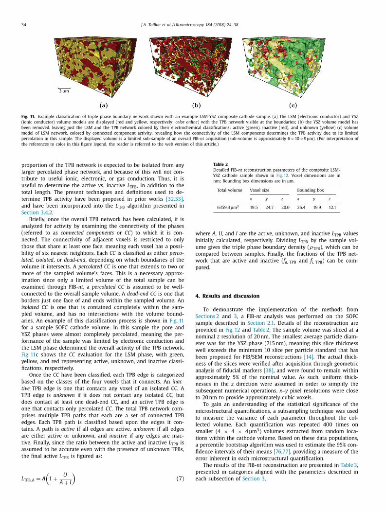
Fig. 11. Example classification of triple phase boundary network shown with an example LSM-YSZ composite cathode sample. (a) The LSM (electronic conductor) and YSZ

(ionic conductor) volume models are displayed (red and yellow, respectively; color online ) with the TPB network visible at the boundaries; (b) the YSZ volume model has

been removed, leaving just the LSM and the TPB network colored by their electrochemical classifications: active (green), inactive (red), and unknown (yellow) (c) volume

model of LSM network, colored by connected component activity, revealing how the connectivity of the LSM components determines the TPB activity due to its limited

percolation in this sample. The displayed volume is a limited sub-sample of an overall FIB- nt acquisition (sub-volume is approximately 6 × 10 × 9 μm). (For interpretation of

the references to color in this figure legend, the reader is referred to the web version of this article.)

Table 2

Detailed FIB- nt reconstruction parameters of the composite LSM-

YSZ cathode sample shown in Fig. 12 . Voxel dimensions are in

nm; Bounding box dimensions are in μm.

Total volume Voxel size Bounding box

x y z x y z

6359.3 μm

3 19.5 24.7 20.0 26.4 19.9 12.1

w

i

u

c

w

p

4

S

s

p

n

e

w

b

n

a

a

n

s

t

m

t

l

s

t

a

fi

e

p

e

proportion of the TPB network is expected to be isolated from any

larger percolated phase network, and because of this will not con-

tribute to useful ionic, electronic, or gas conduction. Thus, it is

useful to determine the active vs. inactive L TPB , in addition to the

total length. The present techniques and definitions used to de-

termine TPB activity have been proposed in prior works [32,33] ,

and have been incorporated into the L TPB algorithm presented in

Section 3.4.2 .

Briefly, once the overall TPB network has been calculated, it is

analyzed for activity by examining the connectivity of the phases

(referred to as connected components or CC ) to which it is con-

nected. The connectivity of adjacent voxels is restricted to only

those that share at least one face, meaning each voxel has a possi-

bility of six nearest neighbors. Each CC is classified as either perco-

lated, isolated , or dead-end , depending on which boundaries of the

volume it intersects. A percolated CC is one that extends to two or

more of the sampled volume’s faces. This is a necessary approx-

imation since only a limited volume of the total sample can be

examined through FIB- nt , a percolated CC is assumed to be well-

connected to the overall sample volume. A dead-end CC is one that

borders just one face of and ends within the sampled volume. An

isolated CC is one that is contained completely within the sam-

pled volume, and has no intersections with the volume bound-

aries. An example of this classification process is shown in Fig. 11

for a sample SOFC cathode volume. In this sample the pore and

YSZ phases were almost completely percolated, meaning the per-

formance of the sample was limited by electronic conduction and

the LSM phase determined the overall activity of the TPB network.

Fig. 11 c shows the CC evaluation for the LSM phase, with green,

yellow, and red representing active, unknown, and inactive classi-

fications, respectively.

Once the CC have been classified, each TPB edge is categorized

based on the classes of the four voxels that it connects. An inac-

tive TPB edge is one that contacts any voxel of an isolated CC . A

TPB edge is unknown if it does not contact any isolated CC , but

does contact at least one dead-end CC, and an active TPB edge is

one that contacts only percolated CC . The total TPB network com-

prises multiple TPB paths that each are a set of connected TPB

edges. Each TPB path is classified based upon the edges it con-

tains. A path is active if all edges are active, unknown if all edges

are either active or unknown, and inactive if any edges are inac-

tive. Finally, since the ratio between the active and inactive L TPB is

assumed to be accurate even with the presence of unknown TPBs,

the final active L TPB is figured as:

L TPB , A = A

(1 +

U

A + I

)(7)

here A, U , and I are the active, unknown, and inactive L TPB values

nitially calculated, respectively. Dividing L TPB by the sample vol-

me gives the triple phase boundary density ( ρTPB ), which can be

ompared between samples. Finally, the fractions of the TPB net-

ork that are active and inactive ( f a , TPB and f i , TPB ) can be com-

ared.

. Results and discussion

To demonstrate the implementation of the methods from

ections 2 and 3 , a FIB- nt analysis was performed on the SOFC

ample described in Section 2.1 . Details of the reconstruction are

rovided in Fig. 12 and Table 2 . The sample volume was sliced at a

ominal z resolution of 20 nm. The smallest average particle diam-

ter was for the YSZ phase (715 nm), meaning this slice thickness

ell exceeds the minimum 10 slice per particle standard that has

een proposed for FIB/SEM reconstructions [14] . The actual thick-

ess of the slices were verified after acquisition through geometric

nalysis of fiducial markers [38] , and were found to remain within

pproximately 5% of the nominal value. As such, uniform thick-

esses in the z direction were assumed in order to simplify the

ubsequent numerical operations. x–y pixel resolutions were close

o 20 nm to provide approximately cubic voxels.

To gain an understanding of the statistical significance of the

icrostructural quantifications, a subsampling technique was used

o measure the variance of each parameter throughout the col-

ected volume. Each quantification was repeated 400 times on

maller (4 × 4 × 4 μm

3 ) volumes extracted from random loca-

ions within the cathode volume. Based on these data populations,

percentile bootstrap algorithm was used to estimate the 95% con-

dence intervals of their means [76,77] , providing a measure of the

rror inherent in each microstructural quantification.

The results of the FIB- nt reconstruction are presented in Table 3 ,

resented in categories aligned with the parameters described in

ach subsection of Section 3 .

J.A. Taillon et al. / Ultramicroscopy 184 (2018) 24–38 35

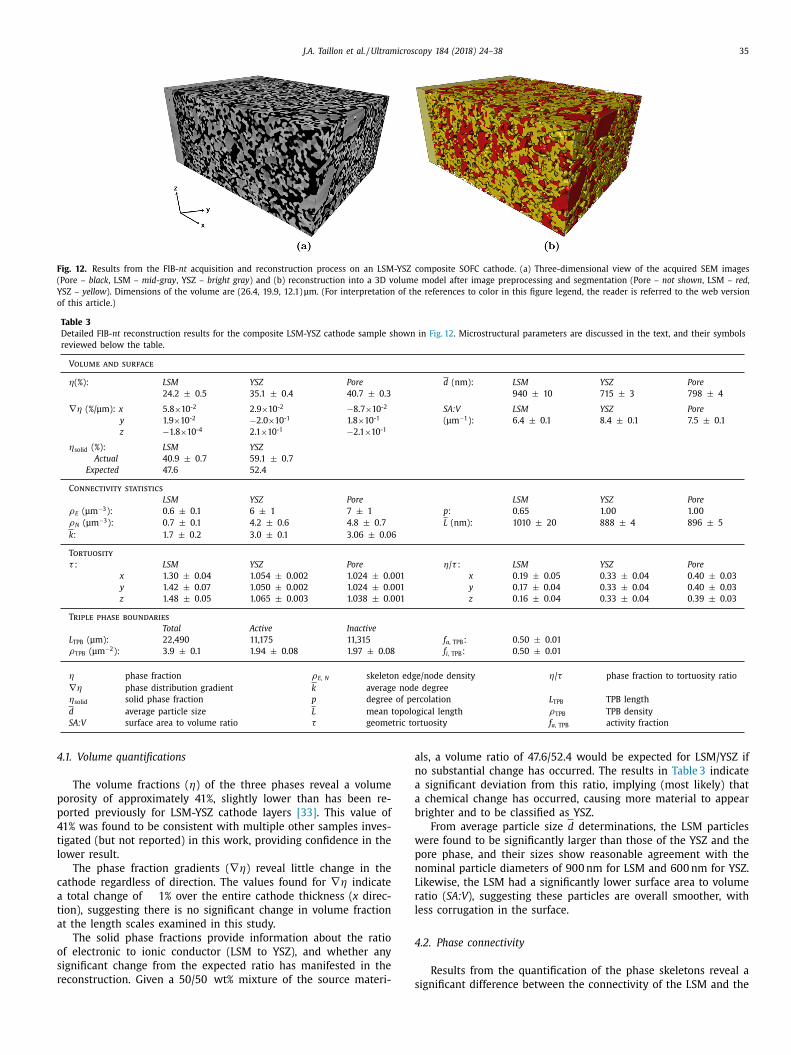
Fig. 12. Results from the FIB- nt acquisition and reconstruction process on an LSM-YSZ composite SOFC cathode. (a) Three-dimensional view of the acquired SEM images

(Pore – black , LSM – mid-gray , YSZ – bright gray ) and (b) reconstruction into a 3D volume model after image preprocessing and segmentation (Pore – not shown , LSM – red ,

YSZ – yellow ). Dimensions of the volume are (26.4, 19.9, 12.1) μm. (For interpretation of the references to color in this figure legend, the reader is referred to the web version

of this article.)

Table 3

Detailed FIB- nt reconstruction results for the composite LSM-YSZ cathode sample shown in Fig. 12 . Microstructural parameters are discussed in the text, and their symbols

reviewed below the table.

Volume and surface

η(%): LSM YSZ Pore d (nm): LSM YSZ Pore

24.2 ± 0.5 35.1 ± 0.4 40.7 ± 0.3 940 ± 10 715 ± 3 798 ± 4

∇η (%/μm): x 5.8 ×10 -2 2.9 ×10 -2 −8.7 ×10 -2 SA:V LSM YSZ Pore

y 1.9 ×10 -2 −2.0 ×10 -1 1.8 ×10 -1 (μm

−1 ): 6.4 ± 0.1 8.4 ± 0.1 7.5 ± 0.1

z −1.8 ×10 -4 2.1 ×10 -1 −2.1 ×10 -1

ηsolid (%): LSM YSZ

Actual 40.9 ± 0.7 59.1 ± 0.7

Expected 47.6 52.4

Connectivity statistics

LSM YSZ Pore LSM YSZ Pore

ρE (μm

−3 ): 0.6 ± 0.1 6 ± 1 7 ± 1 p : 0.65 1.00 1.00

ρN (μm

−3 ): 0.7 ± 0.1 4.2 ± 0.6 4.8 ± 0.7 L (nm): 1010 ± 20 888 ± 4 896 ± 5

k : 1.7 ± 0.2 3.0 ± 0.1 3.06 ± 0.06

Tortuosity

τ : LSM YSZ Pore η/ τ : LSM YSZ Pore

x 1.30 ± 0.04 1.054 ± 0.002 1.024 ± 0.001 x 0.19 ± 0.05 0.33 ± 0.04 0.40 ± 0.03

y 1.42 ± 0.07 1.050 ± 0.002 1.024 ± 0.001 y 0.17 ± 0.04 0.33 ± 0.04 0.40 ± 0.03

z 1.48 ± 0.05 1.065 ± 0.003 1.038 ± 0.001 z 0.16 ± 0.04 0.33 ± 0.04 0.39 ± 0.03

Triple phase boundaries

Total Active Inactive

L TPB (μm): 22,490 11,175 11,315 f a , TPB : 0.50 ± 0.01

ρTPB (μm

−2 ): 3.9 ± 0.1 1.94 ± 0.08 1.97 ± 0.08 f i , TPB : 0.50 ± 0.01

η phase fraction ρE, N skeleton edge/node density η/ τ phase fraction to tortuosity ratio

∇η phase distribution gradient k average node degree

ηsolid solid phase fraction p degree of percolation L TPB TPB length

d average particle size L mean topological length ρTPB TPB density

SA:V surface area to volume ratio τ geometric tortuosity f a , TPB activity fraction

4

p

p

4

t

l

c

a

t

a

o

s

r

a

n

a

a

b

w

p

n

L

r

l

4

.1. Volume quantifications

The volume fractions ( η) of the three phases reveal a volume

orosity of approximately 41%, slightly lower than has been re-

orted previously for LSM-YSZ cathode layers [33] . This value of

1% was found to be consistent with multiple other samples inves-

igated (but not reported) in this work, providing confidence in the

ower result.

The phase fraction gradients ( ∇η) reveal little change in the

athode regardless of direction. The values found for ∇η indicate

total change of � 1% over the entire cathode thickness ( x direc-

ion), suggesting there is no significant change in volume fraction

t the length scales examined in this study.

The solid phase fractions provide information about the ratio

f electronic to ionic conductor (LSM to YSZ), and whether any

ignificant change from the expected ratio has manifested in the

econstruction. Given a 50/50 wt% mixture of the source materi-

s

ls, a volume ratio of 47.6/52.4 would be expected for LSM/YSZ if

o substantial change has occurred. The results in Table 3 indicate

significant deviation from this ratio, implying (most likely) that

chemical change has occurred, causing more material to appear

righter and to be classified as YSZ.

From average particle size d determinations, the LSM particles

ere found to be significantly larger than those of the YSZ and the

ore phase, and their sizes show reasonable agreement with the

ominal particle diameters of 900 nm for LSM and 600 nm for YSZ.

ikewise, the LSM had a significantly lower surface area to volume

atio ( SA:V ), suggesting these particles are overall smoother, with

ess corrugation in the surface.

.2. Phase connectivity

Results from the quantification of the phase skeletons reveal a

ignificant difference between the connectivity of the LSM and the

36 J.A. Taillon et al. / Ultramicroscopy 184 (2018) 24–38

c

f

t

b

q

S

t

t

t

a

t

c

r

r

a

s

r

h

a

c

e

r

D

n

t

o

t

A

d

u

D

n

n

t

I

i

a

t

R

YSZ phases in the present sample. The density of skeleton edges

( ρE ) and nodes ( ρN ) are drastically lower in the LSM than in either

the YSZ or pore phase, meaning it is a simpler phase structure that

can be described with fewer network components. Likewise, the

average node degree ( k ) is correspondingly lower in LSM, suggest-

ing lower connectivity in the phase. The degree of percolation ( p )

indicates that the LSM is poorly connected throughout the volume

(compared to complete percolation of YSZ and the pore), and re-

veals that restricted electronic transport through the LSM will limit

performance of the device. Similarly, the average topological length

( L ) is longest for LSM due to its larger particles with fewer branch-

ing points. All of the connectivity statistics are effectively identical

between the YSZ and pore networks, suggesting that these values

may be common for all fully-percolated phases.

4.3. Tortuosity

The results for tortuosity ( τ ) once again reveal LSM as the

transport limiting phase. Due to its poor connectivity, there was

often a lack of continuous pathway in the LSM throughout the en-

tire sample volume, leading to significantly higher values of τ and

correspondingly higher uncertainties. Within each phase, there is

little change with respect to direction of calculation, demonstrat-

ing the isotropic nature of τ in this sample. There is a slight in-

crease in τ values in the z direction, which is primarily attributed

to the shorter length sampled in that dimension compared to the

others (12.1 μm vs. ∼ 20 μm). This reduced length limits the size

of L E in Eq. (4) , which will lead to larger values of τ (see Fig. 7 d).

The conclusions from measurements of τ are affirmed when con-

sidering the phase fraction to tortuosity ratio ( η/ τ ). This parameter

is expected to be proportional to the effective diffusivity ( Eq. (5) )

and provides a more intuitive insight into how the geometry of

a phase will affect its transport properties. Again, isotropic values

are obtained, with LSM having the lowest η/ τ of the three phases,

yielding reduced conduction through this phase.

4.4. Triple phase boundaries

The total density of triple phase boundary points ( ρTPB ) for this

sample was found to be 3.9 ± 0.1 μm

−2 . Prior theoretical studies re-

garding the dependence of ρTPB on particle size and η indicate that

a value in the range of 2 μm

−2 to 6 μm

−2 would be expected for

the microstructure measured in this work [74] . This indicates the

ρTPB calculation algorithm introduced here produces results that

can be directly compared with other studies.

Both the total ρTPB and the active fraction are significantly de-

pendent on the initial particle size of the source material and the

specific sintering conditions (which control final particle size) [78] .

The active fraction of the TPB network ( f a , TPB ) was found to be 50%

for this sample. Results from a similar LSM-YSZ cathode measured

by Wilson et al. [33] have found higher f a , TPB values (67%), but

their study reconstructed a total cathode volume of only 685 μm

3

(about one-tenth of that studied in this work), suggesting that the

limited volume may artificially inflate measurements of f a , TPB , due

to the definition of activity being dependent on edge connectivity.

This result underscores the importance of collecting a sufficiently

large volume for accurate quantification.

5. Conclusions

FIB- nt is a remarkably powerful technique for measuring ma-

terial microstructures, and is applicable to wide range of sample

types. Analyses of “advanced” microstructural properties such as

tortuosity and triple phase boundary length are of great interest

when it comes to determining the behavior of many material sys-

tems, but are difficult to quantify with currently available commer-

ial and open-source tools. Additionally, specific implementations

rom research are rarely made available to the community, leading

o severe discrepancies between reported methods.

This work has introduced and provided an overview of a num-

er of techniques that can be used to process FIB- nt data and

uantify the microstructural properties of a reconstructed volume.

ignificant advancements have been presented in the correction of

he common FIB-shading artifact, allowing for improved segmen-

ations. Additional improvements in the calculation of microstruc-

ural parameters have been presented, in particular for tortuosity

nd triple phase boundaries. The implementations introduced in

his work have been made available for public use in an online

ode repository, with the intent of allowing peer-review of not only

esults, but methodology as well [30] .

Examples of the calculations discussed in this work have been

eported for an LSM-YSZ SOFC composite cathode layer. The results

re largely in line with prior reports on this system, with the most

ignificant variation apparent in ηsolid and f a , TPB . These calculations

evealed LSM as the transport-limiting phase in this cell, due to its

igh tortuosity and poor connectivity. These results demonstrate

baseline quantification for the LSM-YSZ system, and provide a

ommon and open methodological framework that can be easily

xtended to future FIB- nt reconstructions in a wide range of mate-

ial systems.

isclaimer

Commercial materials and products identified in this article are

ot intended to imply recommendation or endorsement by the Na-

ional Institute of Standards and Technology, nor is the intention

f this article to imply that the materials identified are necessarily

he best available for the stated purpose.

cknowledgments

This project was funded bythe US Department of Energy un-

er NETL Contract DEFE0 0 09084 , and JAT acknowledges support

nder the NSF Graduate Research Fellowship Program, Grant no.

GE1322106 . The authors thank John Hagedorn (Information Tech-

ology Laboratory at the National Institute of Standards and Tech-

ology) for extensive assistance in development and implementa-

ion of the TPB calculation algorithm, as well as Shuo Wang (Trane

ntelligent Services) for conversations inspiring the FIB/SEM shad-

ng correction scheme. The authors also thank Joshua Schumacher

t the Center of Nanoscale Science and Technology (at NIST) for

raining and assistance with FIB/SEM and useful discussions.

eferences

[1] B. Inkson , M. Mulvihill , G. Möbus , 3D determination of grain shape in a

FeAl-based nanocomposite by 3D FIB tomography, Scr. Mater. 45 (2001)753–758 .

[2] FEI Company, Auto Slice & View, for Automated Acquisition of High Reso-lution 3d Images, 2016, ( http://www.fei.com/software/auto- slice- and- view/ ).

(Accessed on 06/03/2016). [3] Zeiss, Atlas 5 – Large Area Imaging for ZEISS SEM, FE-SEM & FIB-SEM,

2016, ( http://www.zeiss.com/microscopy/en _ us/products/microscope-software/

atlas-5.html ). (Accessed on 06/03/2016). [4] Hitachi High Technologies, NanoDUE’T FIB-SEM NB50 0 0, 2016, ( http://

www.hitachi-hightech.com/us/product _ detail/?pn=em-nb50 0 0 ). (Accessed on06/03/2016).

[5] TESCAN, 3d Tomography, 2016, ( http://www.tescan.com/en/other-products/software/3d-tomography ). (Accessed on 06/03/2016).

[6] L. Holzer, M. Cantoni, Review of FIB tomography, Nanofabrication usingFocused Ion and Electron Beams: Principles and Applications, Oxford

University Press, 2012, pp. 410–435 . URL http://books.google.de/books?

id=U- 0mvQcHX5YC&dq=Review+of+FIB- tomography+Lorenz+Holzer&hl= de&source=gbs _ navlinks _ s .

[7] M. Schaffer, J. Wagner, B. Schaffer, M. Schmied, H. Mulders, Automated three-dimensional X-ray analysis using a dual-beam FIB, Ultramicroscopy 107 (2007)

587–597, doi: 10.1016/j.ultramic.20 06.11.0 07 .

J.A. Taillon et al. / Ultramicroscopy 184 (2018) 24–38 37

[

[

[

[

[

[

[

[

[

[

[

[

[

[

[

[

[

[

[

[

[

[

[8] J. Guyon, N. Gey, D. Goran, S. Chalal, F. Pérez-Willard, Advancing FIB assisted3D EBSD using a static sample setup, Ultramicroscopy 161 (2016) 161–167,

doi: 10.1016/j.ultramic.2015.11.011 . [9] P. Burdet, J. Vannod, A. Hessler-Wyser, M. Rappaz, M. Cantoni, Three-

dimensional chemical analysis of laser-welded NiTi-stainless steel wires usinga dual-beam FIB, Acta Mater. 61 (8) (2013) 3090–3098, doi: 10.1016/j.actamat.

2013.01.069 . [10] T. Prill, K. Schladitz, D. Jeulin, M. Faessel, C. Wieser, Morphological segmenta-

tion of FIB-SEM data of highly porous media, J. Microsc. 250 (2) (2013) 77–87,

doi: 10.1111/jmi.12021 . [11] B. Bai, M. Elgmati, H. Zhang, M. Wei, Rock characterization of Fayetteville

shale gas plays, Fuel 105 (2013) 645–652, doi: 10.1016/j.fuel.2012.09.043 . ISSN00162361, URL http://linkinghub.elsevier.com/retrieve/pii/S0 0162361120 07569 .

[12] J.A. Taillon, C. Pellegrinelli, Y. Huang, E. Wachsman, L. Salamanca-Riba,Three dimensional microstructural characterization of cathode degrada-

tion in SOFCs using FIB/SEM and TEM, Microsc. Microanal. 21 (S3)

(2015) 2161–2162 . URL http://journals.cambridge.org/action/displayAbstract? fromPage=online&aid=9916717 .

[13] D. Gostovic, N.J. Vito, K.A. O’Hara, K.S. Jones, E.D. Wachsman, Microstructureand connectivity quantification of complex composite solid oxide fuel cell elec-

trode three-dimensional networks, J. Am. Ceram. Soc. 94 (2) (2011) 620–627,doi: 10.1111/j.1551-2916.2010.04111.x . ISSN 0 0 027820.

[14] L. Holzer, F. Indutnyi, P.H. Gasser, B. Münch, M. Wegmann, Three-dimensional

analysis of porous BaTiO 3 ceramics using FIB nanotomography, J. Microsc. 216(Pt 1) (2004) 84–95, doi: 10.1111/j.0022-2720.2004.01397.x . ISSN 0022-2720,

http://www.ncbi.nlm.nih.gov/pubmed/15369488 . [15] L. Holzer, B. Münch, M. Wegmann, P.H. Gasser, R.J. Flatt, FIB-nanotomography

Of particulate systems - Part I: Particle shape and topology of interfaces, J.Am. Ceram. Soc. 89 (8) (2006) 2577–2585, doi: 10.1111/j.1551-2916.20 06.0 0974.

x . ISSN 0 0 02-7820.

[16] J.R. Wilson, W. Kobsiriphat, R. Mendoza, H.-Y. Chen, J.M. Hiller, D.J. Miller,K. Thornton, P.W. Voorhees, S.B. Adler, S.A. Barnett, Three-dimensional recon-

struction of a solid-oxide fuel-cell anode, Nat. Mater. 5 (7) (2006), doi: 10.1038/nmat1668 . 4–541, ISSN 1476-1122, URL http://www.ncbi.nlm.nih.gov/pubmed/

16767095 . [17] R.K. Bansal, A. Kubis, R. Hull, J.M. Fitz-Gerald, High-resolution three-

dimensional reconstruction: a combined scanning electron microscope and

focused ion-beam approach, J. Vac. Sci. Technol. B 24 (2) (2006) 554,doi: 10.1116/1.2167987 . ISSN 10711023, URL http://link.aip.org/link/JVTBD9/v24/

i2/p554/s1&Agg=doi . [18] D. Gostovic, J.R. Smith, D.P. Kundinger, K.S. Jones, E.D. Wachsman, Three-

dimensional reconstruction of porous LSCF cathodes, Electrochem. Solid-StateLett. 10 (12) (2007) B214, doi: 10.1149/1.2794672 . ISSN 10990062, URL http:

//link.aip.org/link/ESLEF6/v10/i12/pB214/s1&Agg=doi .

[19] J.R. Smith, A. Chen, D. Gostovic, D. Hickey, D.P. Kundinger, K. Duncan, R. De-Hoff, K.S. Jones, E.D. Wachsman, Evaluation of the relationship between cath-

ode microstructure and electrochemical behavior for SOFCs, Solid State Ion-ics 180 (1) (2009) 90–98, doi: 10.1016/j.ssi.2008.10.017 . ISSN 01672738, URL

http://linkinghub.elsevier.com/retrieve/pii/S016727380800619X . 20] D. Gostovic , K.A. O’Hara , N.J. Vito , E.D. Wachsman , K.S. Jones , Multiple length

scale characterization of doped lanthanum manganate composite cathodes,Electrochem. Soc. Trans. 16 (51) (2009) 83–93 .

[21] N. Shikazono, D. Kanno, K. Matsuzaki, H. Teshima, S. Sumino, N. Kasagi, Nu-

merical assessment of SOFC anode polarization based on three-dimensionalmodel microstructure reconstructed from FIB-SEM images, J. Electrochem. Soc.

157 (5) (2010) B665, doi: 10.1149/1.3330568 . ISSN 00134651, URL http://jes.ecsdl.org/cgi/doi/10.1149/1.3330568 .

22] H. Iwai, N. Shikazono, T. Matsui, H. Teshima, M. Kishimoto, R. Kishida,D. Hayashi, K. Matsuzaki, D. Kanno, M. Saito, H. Muroyama, K. Eguchi,

N. Kasagi, H. Yoshida, Quantification of SOFC anode microstructure based on

dual beam FIB-SEM technique, J. Power Sources 195 (4) (2010) 955–961, doi: 10.1016/j.jpowsour.20 09.09.0 05 . ISSN 03787753, URL http://linkinghub.elsevier.

com/retrieve/pii/S0378775309015456 . 23] J. Joos, T. Carraro, A. Weber, E. Ivers-Tiffée, Reconstruction of porous elec-

trodes by FIB/SEM for detailed microstructure modeling, J. Power Sources196 (17) (2011) 7302–7307, doi: 10.1016/j.jpowsour.2010.10.006 . ISSN 03787753,

URL http://linkinghub.elsevier.com/retrieve/pii/S0378775310017337 .

[24] N. Vivet, S. Chupin, E. Estrade, T. Piquero, P. Pommier, D. Rochais, E. Brune-ton, 3D Microstructural characterization of a solid oxide fuel cell anode recon-

structed by focused ion beam tomography, J. Power Sources 196 (18) (2011)7541–7549, doi: 10.1016/j.jpowsour.2011.03.060 . ISSN 03787753, URL http://

linkinghub.elsevier.com/retrieve/pii/S0378775311006756 . 25] G.A. Hughes, K. Yakal-Kremski, A.V. Call, S.A. Barnett, Durability testing of

solid oxide cell electrodes with current switching, J. Electrochem. Soc. 159 (12)

(2012) F858–F863, doi: 10.1149/2.008301jes . ISSN 0013-4651. 26] K.T. Lee, N.J. Vito, E.D. Wachsman, Comprehensive quantification of Ni-

Gd 0.1 Ce 0.9 O 1.95 anode functional layer microstructures by three-dimensionalreconstruction using a FIB/SEM dual beam system, J. Power Sources 228

(2013) 220–228, doi: 10.1016/j.jpowsour.2012.11.117 . ISSN 03787753, URL http://linkinghub.elsevier.com/retrieve/pii/S0378775312018022 .

[27] K. Yakal-Kremski, J.S. Cronin, Y.-C. K. Chen-Wiegart, J. Wang, S.A. Barnett, Stud-

ies of solid oxide fuel cell electrode evolution using 3D tomography, Fuel Cells13 (4) (2013) 449–454, doi: 10.10 02/fuce.20120 0177 . ISSN 16156846.

28] J. Joos, M. Ender, I. Rotscholl, N.H. Menzler, E. Ivers-Tiffée, Quantification ofdouble-layer Ni/YSZ fuel cell anodes from focused ion beam tomography data,

J. Power Sources 246 (2014) 819–830, doi: 10.1016/j.jpowsour.2013.08.021 . ISSN03787753, URL http://linkinghub.elsevier.com/retrieve/pii/S0378775313013608 .

29] H.G. Jones, K.P. Mingard, D.C. Cox, Investigation of slice thickness andshape milled by a focused ion beam for three-dimensional reconstruction

of microstructures, Ultramicroscopy 139 (2014) 20–28, doi: 10.1016/j.ultramic.2014.01.003 . ISSN 18792723, URL http://linkinghub.elsevier.com/retrieve/pii/

S03043991140 0 0138 . 30] J.A. Taillon, Advanced Analytical Microscopy at the Nanoscale: Applications in

Wide Bandgap and Solid Oxide Fuel Cell Materials – FIB- nt Code Repository,

University of Maryland, College Park, 2016 Ph.D. thesis . doi:10.13016/M29806 [31] N.Q. Minh, T. Takahashi, Science and Technology of Ceramic Fuel Cells,

Elsevier, Amsterdam, 1995, doi: 10.1016/B978-04 4 4 8956 8-4/50 0 02-5 . ISBN97804 4 4 8956 84, URL http://www.sciencedirect.com/science/article/pii/

B97804 4 4 8956 8450 0 025 . 32] J.R. Wilson, M. Gameiro, K. Mischaikow, W. Kalies, P.W. Voorhees, S.A. Barnett,

Three-dimensional analysis of solid oxide fuel cell Ni-YSZ anode interconnec-

tivity, Microsc. Microanal. 15 (1) (2009a) 71, doi: 10.1017/S1431927609090096 .ISSN 1431-9276, URL http://www.ncbi.nlm.nih.gov/pubmed/19144260 .

[33] J.R. Wilson, A.T. Duong, M. Gameiro, H.-Y. Chen, K. Thornton, D.R. Mumm,S.A. Barnett, Quantitative three-dimensional microstructure of a solid oxide

fuel cell cathode, Electrochem. Commun. 11 (5) (2009b) 1052–1056, doi: 10.1016/j.elecom.2009.03.010 . ISSN 13882481, URL http://linkinghub.elsevier.com/

retrieve/pii/S1388248109001192 .

34] C.J. Gommes, A.J. Bons, S. Blacher, J.H. Dunsmuir, A.H. Tsou, Practical methodsfor measuring the tortuosity of porous materials from binary or gray-tone to-

mographic reconstructions, AIChE J. 55 (8) (20 09) 20 0 0–2012, doi: 10.1002/aic.11812 . ISSN 0 0 011541.

[35] B. Münch, P. Trtik, F. Marone, M. Stampanoni, Stripe and ring arti-fact removal with combined wavelet-Fourier filtering, Opt. Express

17 (10) (2009) 8567, doi: 10.1364/OE.17.008567 . ISSN 1094- 4087, URL

http://www.ncbi.nlm.nih.gov/pubmed/19434191 http://www.opticsinfobase. org/abstract.cfm?URI=oe- 17- 10- 8567 .

36] D.C. Joy, Control of charging in low-voltage SEM, Scanning 11 (1989) 1–4, doi: 10.1002/sca.4950110102 . ISSN 01610457, URL http://onlinelibrary.wiley.

com/doi/10.1002/sca.4950110102/abstract . [37] K.L. Willis, A.B. Abell, D.A. Lange, Image-based characterization of cement

pore structure using wood metal intrusion, Cem. Concr. Res. 28 (12) (1998)

1695–1705, doi: 10.1016/S0 0 08-8846(98)0 0159-8 . ISSN 0 0 088846, URL http://linkinghub.elsevier.com/retrieve/pii/S0 0 088846980 01598 .

38] E. Principe, Patent, US 8178838, 2012, URL https://www.google.com/patents/US8178838 .

39] J. Schindelin, I. Arganda-Carreras, E. Frise, V. Kaynig, M. Longair, T. Piet-zsch, S. Preibisch, C. Rueden, S. Saalfeld, B. Schmid, J.-Y. Tinevez, D.J. White,

V. Hartenstein, K. Eliceiri, P. Tomancak, A. Cardona, Fiji: an open-source plat-

form for biological-image analysis, Nat. Methods 9 (7) (2012) 676–682, doi: 10.1038/nmeth.2019 .

40] S. van der Walt, S.C. Colbert, G. Varoquaux, The NumPy array: a structure forefficient numerical computation, Comput. Sci. Eng. 13 (2) (2011) 22–30, doi: 10.

1109/mcse.2011.37 . [41] G. Bradski, OpenCV Computer Vision Library, Dr. Dobb’s J. Softw. Tools (20 0 0) .

URL http://www.drdobbs.com/open- source/the- opencv- library/184404319 . 42] S. van der Walt, J.L. Schönberger, J. Nunez-Iglesias, F. Boulogne, J.D. Warner,

N. Yager, E. Gouillart, T. Yu, The scikit-image contributors, scikit-image: image

processing in Python, PeerJ 2 (2014) e453, doi: 10.7717/peerj.453 . ISSN 2167-8359.

43] P. Thévenaz , U. Ruttimann , M. Unser , A pyramid approach to subpixel registra-tion based on intensity, IEEE Trans. Image Process. 7 (1) (1998) 27–41 .

44] M. Schaffer, J. Wagner, Block lift-out sample preparation for 3D experiments ina dual beam focused ion beam microscope, Microchim. Acta 161 (3–4) (2008)

421–425, doi: 10.10 07/s0 0604-0 07- 0853- 5 . ISSN 00263672.

45] X. Dai, The effects of image misregistration on the accuracy of remotely sensedchange detection, IEEE Trans. Geosci. Remote Sens. 36 (5) (1998) 1566–1577,

doi: 10.1109/36.718860 . ISSN 01962892, URL http://ieeexplore.ieee.org/lpdocs/epic03/wrapper.htm?arnumber=718860 .

46] A. Buades, B. Coll, J.-M. Morel, A non-local algorithm for image denoising, in:Proceedings of the 2005 IEEE Computer Society Conference on Computer Vi-

sion and Pattern Recognition, CVPR’05, vol. 2, IEEE, 2005, pp. 60–65, doi: 10.

1109/CVPR.2005.38 . ISBN 0-7695-2372-2, URL http://ieeexplore.ieee.org/lpdocs/epic03/wrapper.htm?arnumber=1467423 .

[47] A. Buades, B. Coll, J.-M. Morel, Non-local means denoising, Image Process. OnLine 1 (2011) 490–530, doi: 10.5201/ipol.2011.bcm _ nlm . URL http://www.ipol.

im/pub/art/2011/bcm _ nlm/ .

48] OpenCV Developers, Image Denoising, 2016. http://docs.opencv.org/master/d5/ d69/tutorial _ py _ non _ local _ means.html .

49] L. Vincent, P. Soille, Watersheds in digital spaces: an efficient algorithm basedon immersion simulations, IEEE Trans. Pattern Anal. Mach. Intell. 13 (6) (1991)

583–598 . ISSN 01628828, doi:10.1109/34.87344 , URL http://ieeexplore.ieee.org/lpdocs/epic03/wrapper.htm?arnumber=87344 .

50] Y. Chen, J.Z. Wang, Image categorization by learning and reasoning with re-gions, J. Mach. Learn. Res. 5 (2004) 913–939 . ISSN 15324435, URL http://portal.

acm.org/citation.cfm?id=1005332.1016789 .

[51] J. Shotton, M. Johnson, R. Cipolla, Semantic texton forests for image cate-gorization and segmentation, in: Proceedings of the 26th IEEE Conference

on Computer Vision and Pattern Recognition, CVPR ISSN 1063-6919, 2008,doi: 10.1109/CVPR.2008.4587503 .

38 J.A. Taillon et al. / Ultramicroscopy 184 (2018) 24–38

[52] M. Rastgarpour , J. Shanbehzadeh , Application of AI techniques in medical im-age segmentation and novel categorization of available methods and tools, in:

Proceedings of the International Multi Conference of Engineers and ComputerScientists, IMECS, 2011, Hong Kong, 1, 2011, pp. 1–6 .

[53] Y. Artan, Interactive image segmentation using machine learning techniques,in: Proceedings of Canadian Conference on Computer and Robot Vision, 2011,

pp. 264–269, doi: 10.1109/CRV.2011.42 . [54] Blender Online Community, Blender – A 3D Modelling and Rendering Pack-

age, Blender Foundation, Blender Institute, Amsterdam, 2016 . URL http://www.

blender.org . [55] W. Schroeder, K. Martin, B. Lorensen, Visualization Toolkit: An Object-Oriented

Approach to 3D Graphics, fourth ed., Kitware, 2006 . ISBN 193093419X, URLhttps://books.google.com/books?id=rx4vPwAACAAJ&dq=isbn:9781930934191

&hl=en&sa=X&ved=0ahUKEwiJmdXc27bLAhWLHh4KHYhuAB8Q6AEIHTAA . [56] S. Brunauer, P.H. Emmett, E. Teller, Adsorption of gases in multimolecular lay-

ers, J. Am. Chem. Soc. 60 (2) (1938) 309–319, doi: 10.1021/ja01269a023 . ISSN

0 0 027863. [57] J.A. Taillon, C. Pellegrinelli, Y. Huang, E.D. Wachsman, L.G. Salamanca-Riba,

Three dimensional microstructural characterization of cathode degradation inSOFCs using focused ion beam and SEM, ECS Trans. 61 (1) (2014) 109–120,

doi: 10.1149/06101.0109ecst . URL http://ecst.ecsdl.org/content/61/1/109.abstract .[58] P.K. Saha, G. Borgefors, G. Sanniti di Baja, A survey on skeletonization algo-

rithms and their applications, Pattern Recognit. Lett. 76 (2016) 312, doi: 10.

1016/j.patrec.2015.04.006 . ISSN 01678655, URL http://www.sciencedirect.com/science/article/pii/S0167865515001233 .

[59] C. Pudney, Distance-ordered homotopic thinning: a skeletonization algo-rithm for 3D digital images, Comput. Vis. Image Underst. 72 (3) (1998)

404–413, doi: 10.1006/cviu.1998.0680 . ISSN 10773142, URL http://linkinghub.elsevier.com/retrieve/pii/S1077314298906804 .

[60] C. Fouard, G. Malandain, S. Prohaska, M. Westerhoff, F. Cassot, C. Mazel,

D. Asselot, J. Marc-Vergnes, Skeletonization by blocks for large 3D datasets:application to brain microcirculation, in: Proceedings of the 2004 2nd

IEEE International Symposium on Biomedical Imaging: Macro to Nano (IEEECat No. 04EX821), vol. 2, IEEE, 2004, pp. 89–92, doi: 10.1109/ISBI.2004.

1398481 . ISBN 0-7803-8388-5, URL http://ieeexplore.ieee.org/lpdocs/epic03/wrapper.htm?arnumber=1398481 .

[61] H.J. Johnson, M. McCormick, L. Ibáñez, T.I.S. Consortium, The ITK Software

Guide, third ed., Kitware, Inc., 2013 . URL http://www.itk.org/ItkSoftwareGuide.pdf .

[62] H. Homann, Implementation of a 3D thinning algorithm, Insight J. (2007) . URLhttp://hdl.handle.net/1926/1292 .

[63] The CGAL Project, CGAL User and Reference Manual, CGAL Editorial Board, 4.7edition, 2015. URL http://doc.cgal.org/4.7/Manual/packages.html .

[64] X. Gao, S. Loriot, A. Tagliasacchi, Triangulated surface mesh skele-

tonization, in: CGAL User and Reference Manual, 4.7 ed., CGALEditorial Board, 2015 . URL http://doc.cgal.org/4.7/Manual/packages.

html#PkgMeanCurvatureSkeleton3Summary . [65] M.B. Clennell, Tortuosity: A Guide Through the Maze, 122(1), Geological Soci-

ety, London, 1997, pp. 299–344, doi: 10.1144/GSL.SP.1997.122.01.18 . Special Pub-lications, ISSN 0305-8719.

[66] G. Brus, K. Miyoshi, H. Iwai, M. Saito, H. Yoshida, Change of an anode’s mi-crostructure morphology during the fuel starvation of an anode-supported

solid oxide fuel cell, Int. J. Hydrogen Energy (2015) 1–8, doi: 10.1016/j.ijhydene.2015.03.143 . ISSN 03603199, URL http://linkinghub.elsevier.com/retrieve/pii/

S0360319915007892 . [67] G. Gaiselmann, M. Neumann, V. Schmidt, O. Pecho, T. Hocker, L. Holzer, Quan-

titative relationships between microstructure and effective transport proper-ties based on virtual materials testing, AIChE J. 60 (6) (2014) 1983–1999,

doi: 10.1002/aic.14416 .

[68] L. Holzer, O. Stenzel, O. Pecho, T. Ott, G. Boiger, M. Gorbar, Y. De Hazan, D. Pen-ner, I. Schneider, R. Cervera, P. Gasser, Fundamental relationships between 3D

pore topology, electrolyte conduction and flow properties: towards knowledge-based design of ceramic diaphragms for sensor applications, Mater. Des. 99

(2016) 314–327, doi: 10.1016/j.matdes.2016.03.034 . [69] O. Stenzel, O. Pecho, L. Holzer, M. Neumann, V. Schmidt, Predicting effective

conductivities based on geometric microstructure characteristics, AIChE J. 62

(5) (2016) 1834–1843, doi: 10.1002/aic.15160 . ISSN 1547-5905, URL http://dx.doi.org/10.1002/aic.15160 .

[70] J.A. Sethian, Fast marching methods, SIAM Rev. 41 (2) (1999) 199–235, doi: 10.1137/S0036144598347059 . ISSN 0036-1445.

[71] J. Furtney, et al., scikit-fmm: The fast marching method for Python (2012) .https://github.com/scikit- fmm/scikit- fmm .

[72] J.-W. Kim, A.V. Virkar, K. Fung, K. Mehta, S.C. Singhal, Polarization effects

in intermediate temperature, anode-supported solid oxide fuel cells, J. Elec-trochem. Soc. 146 (1) (1999) 69, doi: 10.1149/1.1391566 . ISSN 00134651, URL

http://jes.ecsdl.org/cgi/doi/10.1149/1.1391566 . [73] H. Fukunaga, M. Ihara, K. Sakaki, K. Yamada, The relationship between overpo-

tential and the three phase boundary length, Solid State Ionics 86–88 (Part 2)(1996) 1179–1185, doi: 10.1016/0167- 2738(96)00284- 6 . ISSN 01672738.

[74] B. Kenney, M. Valdmanis, C. Baker, J. Pharoah, K. Karan, Computation of

TPB length, surface area and pore size from numerical reconstruction ofcomposite solid oxide fuel cell electrodes, J. Power Sources 189 (2) (2009)

1051–1059, doi: 10.1016/j.jpowsour.2008.12.145 . ISSN 03787753, URL http://linkinghub.elsevier.com/retrieve/pii/S03787753090 0 0378 .

[75] J.R. Wilson, S.A. Barnett, Solid oxide fuel cell Ni-YSZ anodes: Effect of com posi-tion on microstructure and performance, Electrochem. Solid-State Lett. 11 (10)

(2008) B181, doi: 10.1149/1.2960528 . ISSN 10990062.

[76] B. Efron, R. Tibshirani, An Introduction to the Bootstrap (Chapman &Hall/CRC Monographs on Statistics & Applied Probability), Chapman

and Hall/CRC, 1994 . ISBN 0412042312, URL http://www.amazon.com/Introduction-Bootstrap-Monographs-Statistics-Probability/dp/0412042312%

3FSubscriptionId%3D0JYN1NVW651KCA56C102%26tag%3Dtechkie-20% 26linkCode%3Dxm2%26camp%3D2025%26creative%3D165953%26creativeASIN%

3D0412042312 .

[77] C. Evans, scikits-bootstrap: Bootstrap confidence interval algorithms for scipy,2012, https://github.com/cgevans/scikits-bootstrap .

[78] J.S. Cronin, K. Muangnapoh, Z. Patterson, K.J. Yakal-Kremski, V.P. Dravid,S.A. Barnett, Effect of firing temperature on LSM-YSZ composite cathodes:

a combined three-dimensional microstructure and impedance spectroscopystudy, J. Electrochem. Soc. 159 (4) (2012) B385, doi: 10.1149/2.053204jes .