Embed Size (px)
Citation preview
Computational Models for Auditory Scene Analysis
by
Shariq A. Mobin
A dissertation submitted in partial satisfaction of the
requirements for the degree of
Doctor of Philosophy
in
Neuroscience
in the
Graduate Division
of the
University of California, Berkeley
Committee in charge:
Professor Bruno Olshausen, ChairProfessor Frederic Theunissen
Professor Michael YartsevProfessor Michael DeWeese
Spring 2019
Computational Models for Auditory Scene Analysis
Copyright 2019by
Shariq A. Mobin
1
Abstract
Computational Models for Auditory Scene Analysis
by
Shariq A. Mobin
Doctor of Philosophy in Neuroscience
University of California, Berkeley
Professor Bruno Olshausen, Chair
The high levels goals of this thesis are to: understand the neural representation of sound,produce more robust statistical models of natural sound, and develop models for top-downauditory attention. These are three critical concepts in the auditory system. The neuralrepresentation of sound should provide a useful representation for building robust statisticalmodels and directing attention. Robust statistical models are necessary for humans to gen-eralize their knowledge from one domain to the plethora of domains in the real world. Andattention is fundamental to the perception of sound, allowing one to prioritize informationin the raw audio signal.
First, I approach understanding the neural representation of sound using the efficientcoding principle and the physiological characteristics of the cochlea. A theoretical modelis developed using convolutional filters and leaky-integrate-and-fire (LIF) neurons to modelthe cochlear transform and spiking code of the auditory nerve. The goal of this model is toexplain the distributed phase code of the auditory nerve response but it lays the foundationfor much more.
Second, I investigate an algorithm for audio source separation, called deep clustering. Ex-periments are performed to evaluate it’s robustness, and a new neural network architectureis developed to improve robustness. The experiments show that the conventional recur-rent neural network performs sub-optimally, and our dilated convolutional neural networkimproves robustness while using an order of magnitude fewer parameters. This more parsi-monious model is a step towards models which are minimally parameterized and generalizewell across many domains.
Third, I develop a new algorithm to address the limitations of the previous deep clusteringmethod. This algorithm can extract multiple sources at once from a mixture using anattentional context or bias. It relies on modulating the computation of the bottom-uppathway using a top-down neural signal, which indicates which sources are of interest. Asimple idea from the attentional spotlight method is used to do this: to allow for the top-down neural signal to modulate the gain on a set of low level neurons. This computationalmethod demonstrates one way top-down feedback could direct auditory attention in the
2
brain. Interestingly, this method goes beyond neuroscience, it demonstrates that attentioncan be about more than efficient computation. The experiments show that it resolves one ofthe main short comings of deep clustering. The model can extract sources from a mixturewithout knowing the total number of sources in the mixture, unlike deep clustering.
The major contributions of this work are a theoretical model for the auditory nerveresponse, a more robust neural network architecture for sound understanding, and a noveland powerful model of top-down auditory attention. I hope that the first contribution willbe used to build a better understanding of the complex auditory nerve code. The secondto build ever more parsimonious and robust models of source separation. And the third toprovide a basis for an under-explored research direction which I believe is the most fruitfulfor building human-level auditory scene analysis, attention-based source separation.
i
Acknowledgments
I thank my father for instilling in me perseverance, curiosity, and to have borderline crazydreams. My mother for humility, levelheadedness, and independence. My brother for craftythinking, intelligence, and a passion for science and technology. And all of them for theirundying support and encouragement over the many years of my education.
I thank Bruno Olshausen, my advisor, for teaching me how to be a great scientist, toask the right questions, and to dive deeper into subjects. His continuing love of knowledge,passion for inspiring new scientists, and excitement for the future all make the RedwoodCenter an incredible place to occupy. His ideas and perspectives inspire much of my work.
I thank Brian Cheung for being an incredible friend and collaborator. I spent countlesshours bouncing ideas off Brian over the years and his insights were instrumental to mysuccess.
I thank my thesis committee for their feedback and encouragement of my work. MikeDeweese for his astounding excitement, Frederic Theunissen for his pointed comments, andMichael Yartsev for his continued support.
I thank the entire Redwood Center for Theoretical Neuroscience. The Redwood is full ofbrilliant neuroscientists, statisticians, and physicists who have all contributed a great dealto my scientific skill set. Special thanks to Fritz Sommer who provided early guidance andencouragement to me, leading me to publish my first machine learning paper. I also wantto thank my colleagues Alex Anderson, Yubei Chen, Jasmine Collins, Charles Frye, DylanPaiton, Sophia Sanborn, and Eric Weiss for excellent discussions and banter that kept megoing.
To my outside mentor, Dick Lyon, for teaching me about the real-world implications ofmy research and connecting me with brilliant engineers and scientists at Google Brain.
And finally to all my friends in the Helen Wills Neuroscience Institute and the Bay Area.Especially Shomik Chakravarty, Irene Grossrubatscher, Maimon Rose, Andrew Saada, DanielSaltiel, and Jessie Temple for their incredible friendship and energy.
ii
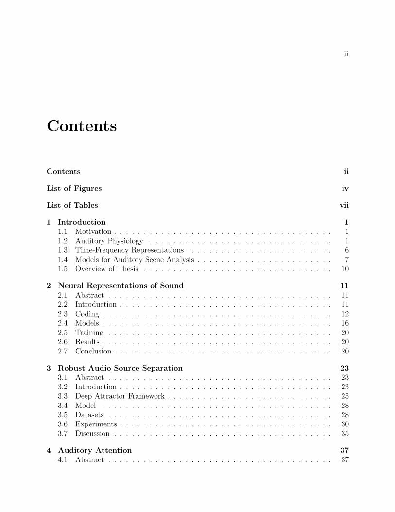
Contents
Contents ii
List of Figures iv
List of Tables vii
1 Introduction 11.1 Motivation . . . . . . . . . . . . . . . . . . . . . . . . . . . . . . . . . . . . . 11.2 Auditory Physiology . . . . . . . . . . . . . . . . . . . . . . . . . . . . . . . 11.3 Time-Frequency Representations . . . . . . . . . . . . . . . . . . . . . . . . 61.4 Models for Auditory Scene Analysis . . . . . . . . . . . . . . . . . . . . . . . 71.5 Overview of Thesis . . . . . . . . . . . . . . . . . . . . . . . . . . . . . . . . 10
2 Neural Representations of Sound 112.1 Abstract . . . . . . . . . . . . . . . . . . . . . . . . . . . . . . . . . . . . . . 112.2 Introduction . . . . . . . . . . . . . . . . . . . . . . . . . . . . . . . . . . . . 112.3 Coding . . . . . . . . . . . . . . . . . . . . . . . . . . . . . . . . . . . . . . . 122.4 Models . . . . . . . . . . . . . . . . . . . . . . . . . . . . . . . . . . . . . . . 162.5 Training . . . . . . . . . . . . . . . . . . . . . . . . . . . . . . . . . . . . . . 202.6 Results . . . . . . . . . . . . . . . . . . . . . . . . . . . . . . . . . . . . . . . 202.7 Conclusion . . . . . . . . . . . . . . . . . . . . . . . . . . . . . . . . . . . . . 20
3 Robust Audio Source Separation 233.1 Abstract . . . . . . . . . . . . . . . . . . . . . . . . . . . . . . . . . . . . . . 233.2 Introduction . . . . . . . . . . . . . . . . . . . . . . . . . . . . . . . . . . . . 233.3 Deep Attractor Framework . . . . . . . . . . . . . . . . . . . . . . . . . . . . 253.4 Model . . . . . . . . . . . . . . . . . . . . . . . . . . . . . . . . . . . . . . . 283.5 Datasets . . . . . . . . . . . . . . . . . . . . . . . . . . . . . . . . . . . . . . 283.6 Experiments . . . . . . . . . . . . . . . . . . . . . . . . . . . . . . . . . . . . 303.7 Discussion . . . . . . . . . . . . . . . . . . . . . . . . . . . . . . . . . . . . . 35
4 Auditory Attention 374.1 Abstract . . . . . . . . . . . . . . . . . . . . . . . . . . . . . . . . . . . . . . 37
iii
4.2 Introduction . . . . . . . . . . . . . . . . . . . . . . . . . . . . . . . . . . . . 374.3 Multi-Speaker Extraction . . . . . . . . . . . . . . . . . . . . . . . . . . . . . 394.4 Experiments . . . . . . . . . . . . . . . . . . . . . . . . . . . . . . . . . . . . 434.5 Discussion . . . . . . . . . . . . . . . . . . . . . . . . . . . . . . . . . . . . . 46
5 Conclusion 485.1 Closing remarks . . . . . . . . . . . . . . . . . . . . . . . . . . . . . . . . . . 485.2 Next Steps . . . . . . . . . . . . . . . . . . . . . . . . . . . . . . . . . . . . . 49
Bibliography 50
iv
List of Figures
1.1 Five individual voltage recordings of sensory hair cells, each in response to a puresinusoidal frequencies indicated on the right. If you count the peaks, you willnotice that the voltage oscillates at the frequency of the stimulus. Image adaptedfrom [52]. . . . . . . . . . . . . . . . . . . . . . . . . . . . . . . . . . . . . . . . 3
1.2 Normalized firing rate along the auditory nerve in response to auditory stimuluspresented at different volumes (dB SPL). The colors indicate what volume thecochlea was allowed to adapt to before performing the volume sweep. When thecochlea adapts to loud volumes the curve shifts right but the shape of the curveremains similar. Adapted from [69]. . . . . . . . . . . . . . . . . . . . . . . . . . 3
1.3 Frequency tuning curves of several auditory nerve fibers. Each point on a curvecorresponds to the minimum sound level required to record a threshold numberof spikes from the fiber. Adapted from [16] . . . . . . . . . . . . . . . . . . . . . 4
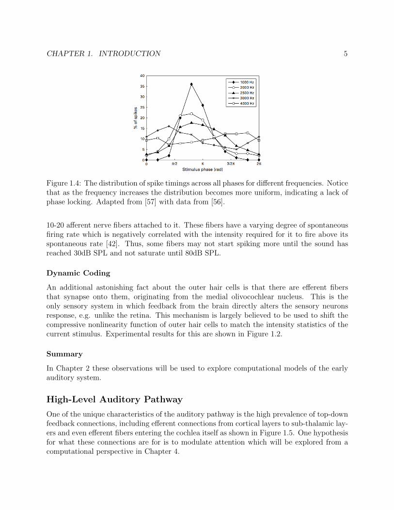
1.4 The distribution of spike timings across all phases for different frequencies. Noticethat as the frequency increases the distribution becomes more uniform, indicatinga lack of phase locking. Adapted from [57] with data from [56]. . . . . . . . . . 5
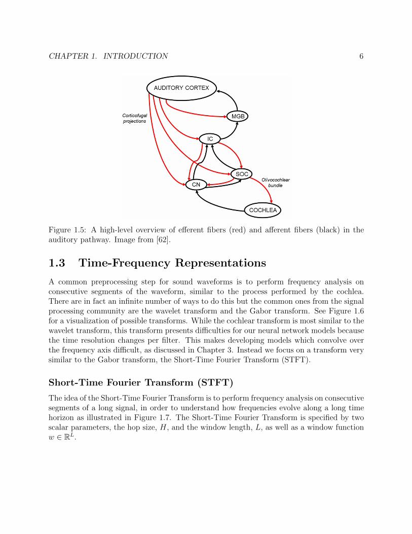
1.5 A high-level overview of efferent fibers (red) and afferent fibers (black) in theauditory pathway. Image from [62]. . . . . . . . . . . . . . . . . . . . . . . . . . 6
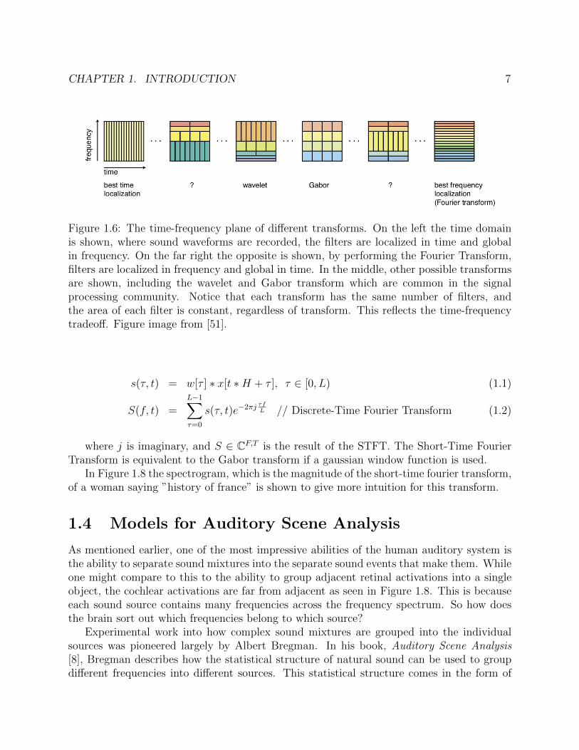
1.6 The time-frequency plane of different transforms. On the left the time domain isshown, where sound waveforms are recorded, the filters are localized in time andglobal in frequency. On the far right the opposite is shown, by performing theFourier Transform, filters are localized in frequency and global in time. In themiddle, other possible transforms are shown, including the wavelet and Gabortransform which are common in the signal processing community. Notice thateach transform has the same number of filters, and the area of each filter is con-stant, regardless of transform. This reflects the time-frequency tradeoff. Figureimage from [51]. . . . . . . . . . . . . . . . . . . . . . . . . . . . . . . . . . . . . 7
1.7 Diagram of the Short-Time Fourier Transform process as well as it’s inverse.In this diagram H = L
2. The analysis consists of segmenting the waveform,
multiplying by a window, and taking the fourier transform. The synthesis consistsof the inverse operations. Figure image from [59]. . . . . . . . . . . . . . . . . . 8
v
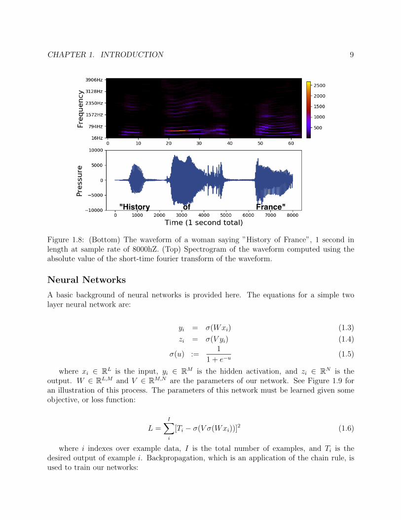
1.8 (Bottom) The waveform of a woman saying ”History of France”, 1 second inlength at sample rate of 8000hZ. (Top) Spectrogram of the waveform computedusing the absolute value of the short-time fourier transform of the waveform. . . 9
1.9 Diagram for a 2 layer neural network. . . . . . . . . . . . . . . . . . . . . . . . . 10
2.1 The kernel functions resemble gammatone filters (red). Matching teverse Corre-lation (revcor) filters found from the auditory nerve response of chinchillas [55]are shown in blue. From Smith and Lewicki [61]. . . . . . . . . . . . . . . . . . 15
2.2 A spectrogram-like representation of the input stimulus using the optimal kernelsand coefficients. The kernels are ordered vertically by their center frequency.Colors simply denote different kernels in this diagram. From [61]. . . . . . . . . 16
2.3 Bottom - A spectrogram-like representation of speech from the GRID SpeechCorpus using wavelets (similar to gammatone filters) with overlapping receptivefields. Top - An artificial spike based representation using these filters. Note thatthe sound stimulus is represented in a highly distributed way, there are 5 artificialfibers firing in response to the fundamental frequency contained in the stimulus. 17
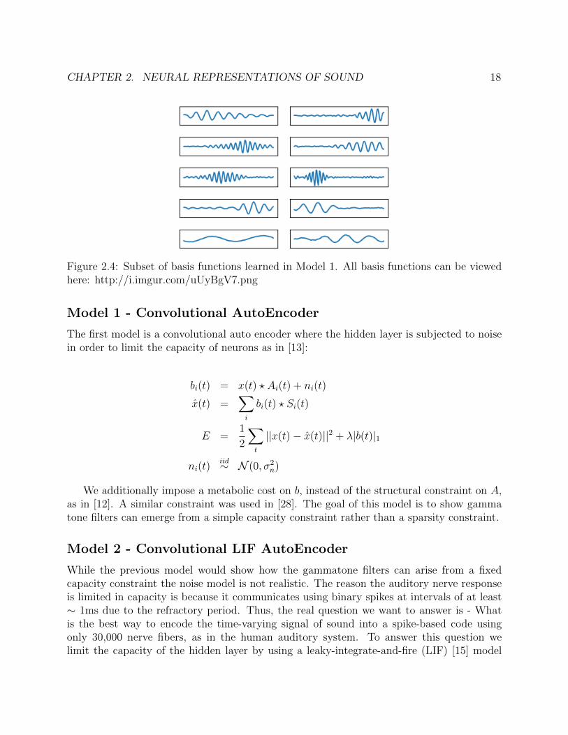
2.4 Subset of basis functions learned in Model 1. All basis functions can be viewedhere: http://i.imgur.com/uUyBgV7.png . . . . . . . . . . . . . . . . . . . . . . 18
2.5 Diagram of the model. Inner Hair Cell (IHC). Auditory Nerve (AN). . . . . . . 192.6 A smoothed version of the spike activation function that allows for easier gradient
based optimization . . . . . . . . . . . . . . . . . . . . . . . . . . . . . . . . . . 212.7 A smoothed version of the voltage reset function that allows for easier gradient
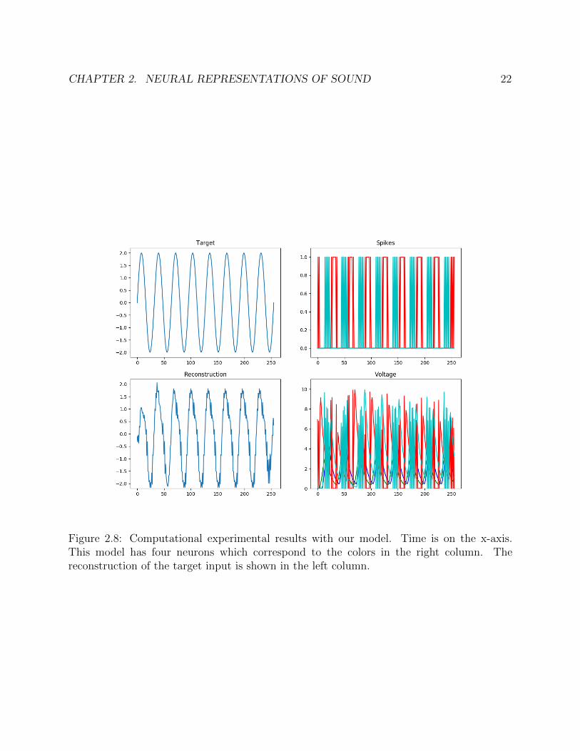
based optimization . . . . . . . . . . . . . . . . . . . . . . . . . . . . . . . . . . 212.8 Computational experimental results with our model. Time is on the x-axis. This
model has four neurons which correspond to the colors in the right column. Thereconstruction of the target input is shown in the left column. . . . . . . . . . . 22
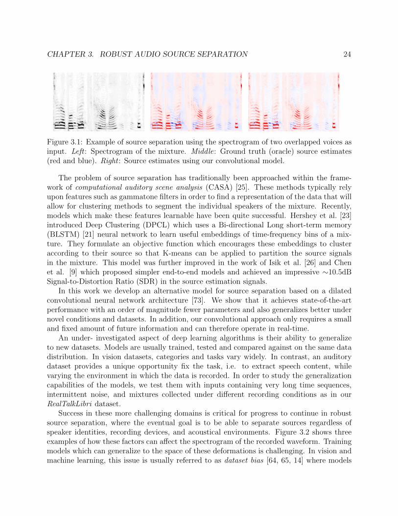
3.1 Example of source separation using the spectrogram of two overlapped voices asinput. Left : Spectrogram of the mixture. Middle: Ground truth (oracle) sourceestimates (red and blue). Right : Source estimates using our convolutional model. 24
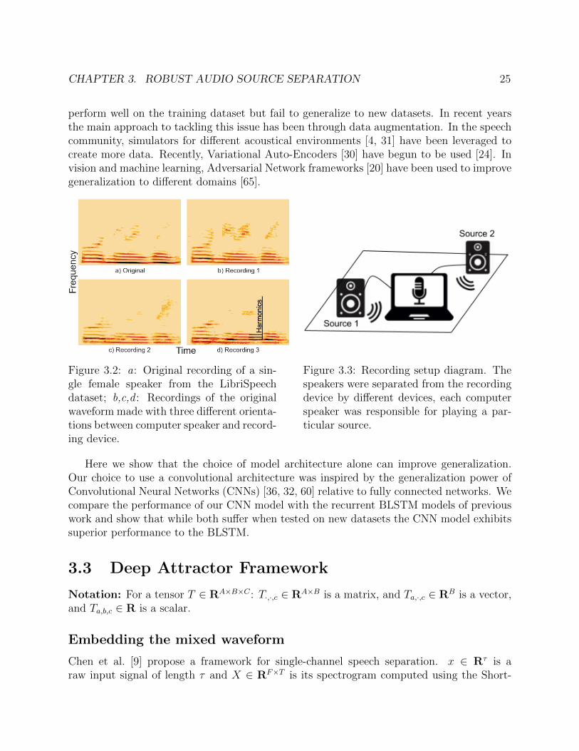
3.2 a: Original recording of a single female speaker from the LibriSpeech dataset;b,c,d : Recordings of the original waveform made with three different orientationsbetween computer speaker and recording device. . . . . . . . . . . . . . . . . . . 25
3.3 Recording setup diagram. The speakers were separated from the recording de-vice by different devices, each computer speaker was responsible for playing aparticular source. . . . . . . . . . . . . . . . . . . . . . . . . . . . . . . . . . . . 25
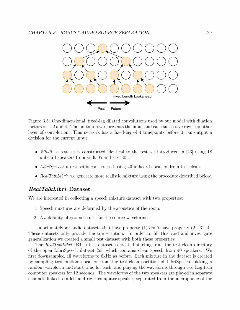
3.4 Overview of the source separation process. . . . . . . . . . . . . . . . . . . . . . 273.5 One-dimensional, fixed-lag dilated convolutions used by our model with dilation
factors of 1, 2 and 4. The bottom row represents the input and each successiverow is another layer of convolution. This network has a fixed-lag of 4 timepointsbefore it can output a decision for the current input. . . . . . . . . . . . . . . . 29
vi
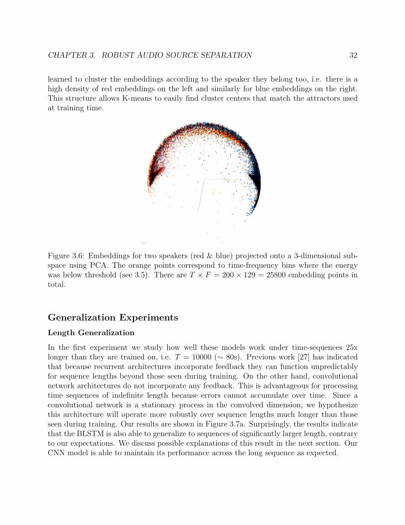
3.6 Embeddings for two speakers (red & blue) projected onto a 3-dimensional sub-space using PCA. The orange points correspond to time-frequency bins wherethe energy was below threshold (see 3.5). There are T × F = 200× 129 = 25800embedding points in total. . . . . . . . . . . . . . . . . . . . . . . . . . . . . . 32
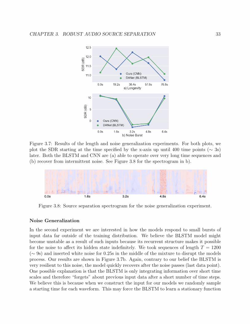
3.7 Results of the length and noise generalization experiments. For both plots, weplot the SDR starting at the time specified by the x-axis up until 400 time points(∼ 3s) later. Both the BLSTM and CNN are (a) able to operate over very longtime sequences and (b) recover from intermittent noise. See Figure 3.8 for thespectrogram in b). . . . . . . . . . . . . . . . . . . . . . . . . . . . . . . . . . . 33
3.8 Source separation spectrogram for the noise generalization experiment. . . . . . 333.9 Results of the models tested on WSJ0 simulated mixtures, LibriSpeech simulated
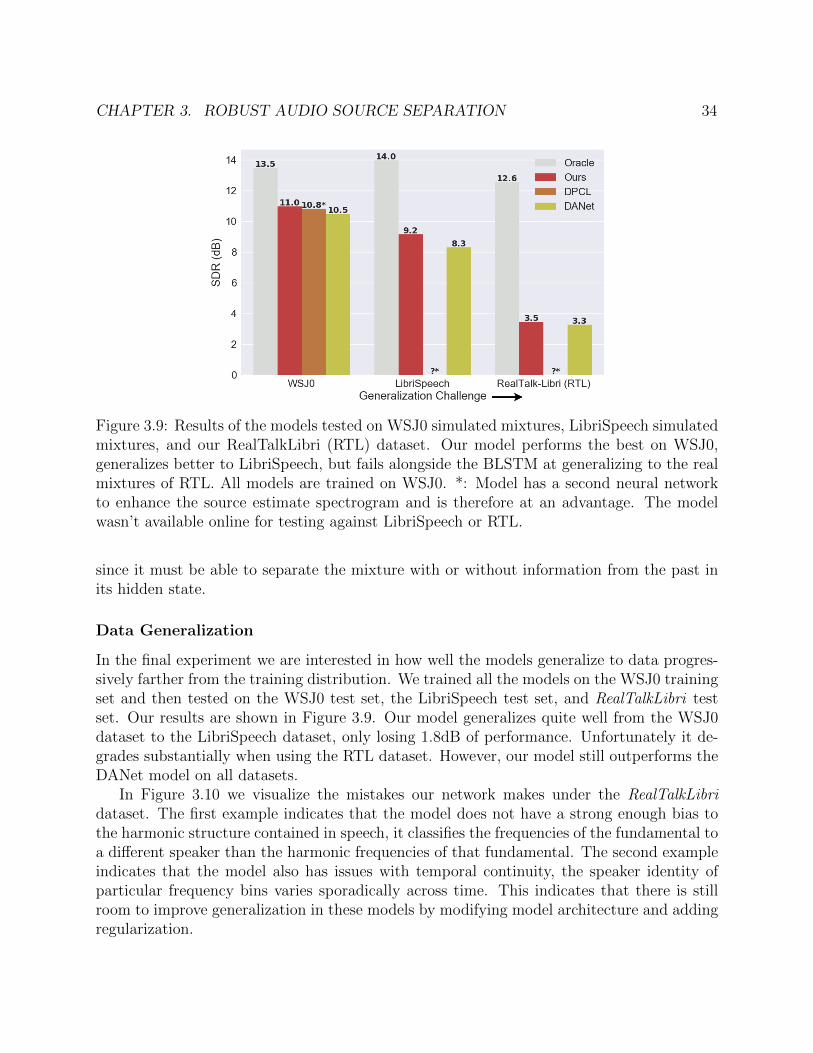
mixtures, and our RealTalkLibri (RTL) dataset. Our model performs the beston WSJ0, generalizes better to LibriSpeech, but fails alongside the BLSTM atgeneralizing to the real mixtures of RTL. All models are trained on WSJ0. *:Model has a second neural network to enhance the source estimate spectrogramand is therefore at an advantage. The model wasn’t available online for testingagainst LibriSpeech or RTL. . . . . . . . . . . . . . . . . . . . . . . . . . . . . . 34
3.10 Left and right column: Two examples of source separation on the RealTalkLibridataset. Row 1 : Source estimates using the oracle. Row 2 : The source estimatesusing our method. The model has difficulty maintaining continuity of speakeridentity across frequencies of a harmonic stack (left column) and across time(right column). . . . . . . . . . . . . . . . . . . . . . . . . . . . . . . . . . . . . 35
4.1 Overview of the attention-based multi-speaker separation process. Circles denoteoperations and rounded squares represent variables. In this diagram G=3, H=3,and N=7, see text for details. Components colored in green represent supervisedinformation about the desired target speaker. Purple indicates the compressedspectrogram, orange the model, and red the loss. fc corresponds to the compres-sion function used. . . . . . . . . . . . . . . . . . . . . . . . . . . . . . . . . . . 41
4.2 LSTM-Append Model. The target specification is encoded in the vector B. Toincorporate this into the network B is appended to the normal input at each timestep. . . . . . . . . . . . . . . . . . . . . . . . . . . . . . . . . . . . . . . . . . . 42
vii
List of Tables
3.1 Dilated Convolutional Network Architecture . . . . . . . . . . . . . . . . . . . . 303.2 SDR for two competitor models, our proposed convolutional model, and the Or-
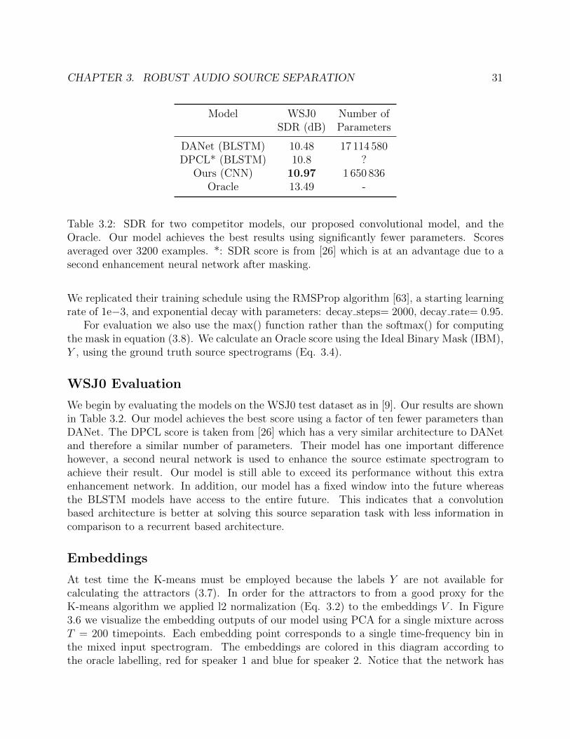
acle. Our model achieves the best results using significantly fewer parameters.Scores averaged over 3200 examples. *: SDR score is from [26] which is at anadvantage due to a second enhancement neural network after masking. . . . . . 31
4.1 Model hyperparamters . . . . . . . . . . . . . . . . . . . . . . . . . . . . . . . . 444.2 SDR of our method on the known-eval partition compared to deep clustering
results from Mobin et al. [48] on the test-clean partitions of LibriSpeech. Whilethese partitions are not identical they come from the same dataset and are com-parable. . . . . . . . . . . . . . . . . . . . . . . . . . . . . . . . . . . . . . . . . 45
4.3 SDR for the Phase 2 fine-tuning on the new speakers. Results are compared tothe baseline attention network of Xiao et al. [71] . . . . . . . . . . . . . . . . . . 45
4.4 SDR for our Phase 1 training on known speakers where there are multiple targetsand interferers. No other neural network model is capable of working on this task. 46
1
Chapter 1
Introduction
1.1 Motivation
A number of questions have puzzled me during my study of auditory neuroscience. 1) Whydoes the cochlea choose to represent sound in a time-frequency representation? 2) How dowe build human-level robust statistical models of sound? 3) What role does feeback playin attention? While tackling all these problems may seem daunting at first, the belief thatthe brain computes the most parsimonious model of sound to accomplish a behaviour goalcan be quite powerful. But what should that behavioural goal be? One difficulty that allanimals face is that the sound waveform that enters our ears is often a mixture of manyindividual sources. Yet our conscious experience of sound is made up of the individualsources themselves, demixed, which is critical to our survival. In much of my research I willmake progress on these three questions by using a combination of learning algorithms, largemodels that make efficient use of their parameters, lots of data, and this behavioural goal.In this chapter, I provide background on the physiology of the auditory pathway, discussdifferent representations of sound, and finally review the idea of auditory scene analysis andhow neural networks can be applied to it.
1.2 Auditory Physiology
In this section background knowledge on the physiology of the cochlea as well as some detailsof the entire auditory pathway are provided. The information in this section informs thetheoretical model in Chapter 2 but is not required for understanding it, nor the remainingthe chapters.

CHAPTER 1. INTRODUCTION 2
Subcortical Physiology
The Mechanical Representation of Sound
Sound vibrations enter the ear canal and cause vibrations of the ear drum. These vibrationsare then amplified by three bones, the Malleus, Incus, and Stapes in order to amplify theinput signal in preparation for the fluid-filled chamber of the cochlea. The cochlea acts amechanical frequency analyzer through the mechanical properties of the basilar membraneand fluids that fill it. The basilar membrane is narrow and stiff at the basal end of thecochlea but progressively more wide and floppy towards the apical end. This mechanicalproperty leads high frequencies to vibrate more basal parts of the basilar membrane while lowfrequencies vibrate more apical ends. Thus, if the input waveform contains a single frequencythen the place of maximal vibration in the basilar membrane gives a good indication of whatfrequency is contained within the signal. Because of the frequency analysis property of thecochlea it is often described as a biological Fourier analyzer. However, if the cochlea isthought of as a set of mechanical filters, they differ in some fundamental ways as comparedto the Fourier filters. These differences include the logarithmic frequency spacing of thecochlear filters as well as their tuning bandwidth being approximately one-sixth of the centerfrequency of the filter. To address these differences and more, a gamma-tone filter bank istypically used. It is important to note that modeling the cochlea using this filter followsfrom a linear assumption about the cochlea which is not true. This will become clear a littlelater. However, in practice, this assumption is a reasonable first approximation.
Transduction: From Vibrations to Voltage
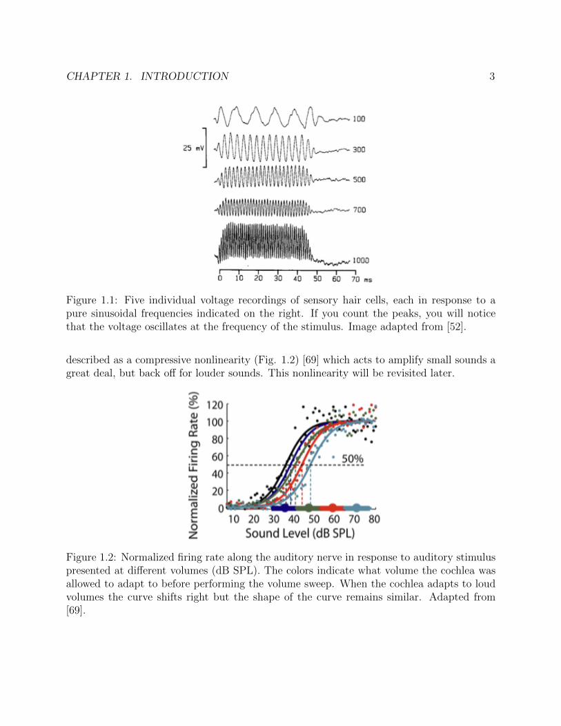
The next stage of auditory processing is the conversion of vibrations in the basilar membraneinto a voltage change of the spiral ganglion. This conversion takes place in the Organ ofCorti, a structure attached to the basilar membrane. Inside the Organ of Corti lie sensoryhair cells which are the specific components that transduce the mechanical vibrations. Theyaccomplish this task through small hairs called stereocilia which sit on top of them. Thesehairs form mechano-gated potassium channels with the sensory hair cells. That is, in responseto vibrations, these stereocilias sway back and forth, causing a potassium channel to openwhich depolarizes the hair cells. The hair cells voltage will then mimic the basilar membranesvibration as an alternating current (AC), at least up to 1kHz (Fig. 1.1) [52].
Up until now all hair cells have been treated as equivalent. However, an importantdistinction is made between inner hair cells (IHCs) and outer hair cells (OHCs). Inner haircells are purely sensory neurons which simply act to transduce the vibrations of the basilarmembrane. Outer hair cells also transduce these vibrations but have an additional astoundingproperty - they oscillate the lengths of their cell bodies according to their membrane voltage,thus providing a feedback amplification process. This amplification process is critical to ourability to discriminate between small changes in frequency as well as our ability to hearsounds at the enormous range of over 120dB [66]. Mathematically, this amplification is often
CHAPTER 1. INTRODUCTION 3
Figure 1.1: Five individual voltage recordings of sensory hair cells, each in response to apure sinusoidal frequencies indicated on the right. If you count the peaks, you will noticethat the voltage oscillates at the frequency of the stimulus. Image adapted from [52].
described as a compressive nonlinearity (Fig. 1.2) [69] which acts to amplify small sounds agreat deal, but back off for louder sounds. This nonlinearity will be revisited later.
Figure 1.2: Normalized firing rate along the auditory nerve in response to auditory stimuluspresented at different volumes (dB SPL). The colors indicate what volume the cochlea wasallowed to adapt to before performing the volume sweep. When the cochlea adapts to loudvolumes the curve shifts right but the shape of the curve remains similar. Adapted from[69].
CHAPTER 1. INTRODUCTION 4
Spikes: From Voltage Fluctuations to Action Potentials
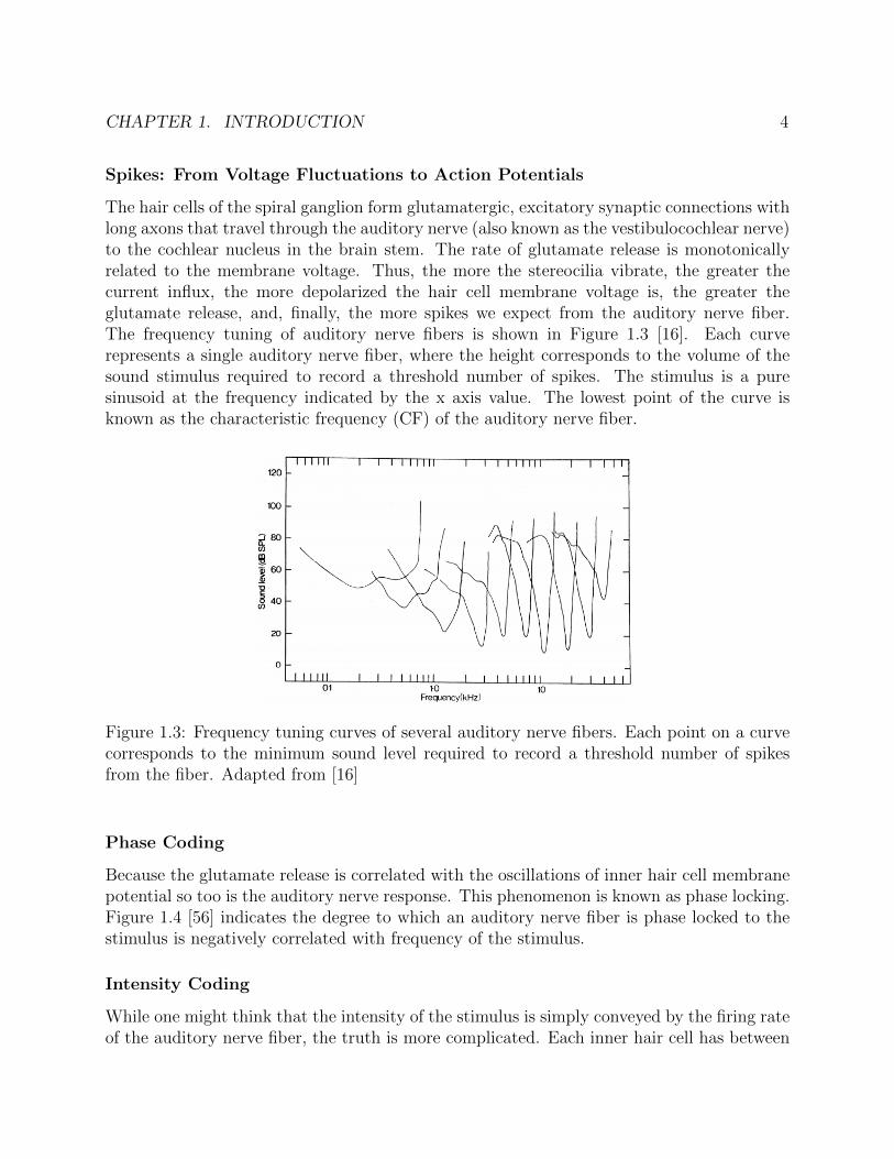
The hair cells of the spiral ganglion form glutamatergic, excitatory synaptic connections withlong axons that travel through the auditory nerve (also known as the vestibulocochlear nerve)to the cochlear nucleus in the brain stem. The rate of glutamate release is monotonicallyrelated to the membrane voltage. Thus, the more the stereocilia vibrate, the greater thecurrent influx, the more depolarized the hair cell membrane voltage is, the greater theglutamate release, and, finally, the more spikes we expect from the auditory nerve fiber.The frequency tuning of auditory nerve fibers is shown in Figure 1.3 [16]. Each curverepresents a single auditory nerve fiber, where the height corresponds to the volume of thesound stimulus required to record a threshold number of spikes. The stimulus is a puresinusoid at the frequency indicated by the x axis value. The lowest point of the curve isknown as the characteristic frequency (CF) of the auditory nerve fiber.
Figure 1.3: Frequency tuning curves of several auditory nerve fibers. Each point on a curvecorresponds to the minimum sound level required to record a threshold number of spikesfrom the fiber. Adapted from [16]
Phase Coding
Because the glutamate release is correlated with the oscillations of inner hair cell membranepotential so too is the auditory nerve response. This phenomenon is known as phase locking.Figure 1.4 [56] indicates the degree to which an auditory nerve fiber is phase locked to thestimulus is negatively correlated with frequency of the stimulus.
Intensity Coding
While one might think that the intensity of the stimulus is simply conveyed by the firing rateof the auditory nerve fiber, the truth is more complicated. Each inner hair cell has between
CHAPTER 1. INTRODUCTION 5
Figure 1.4: The distribution of spike timings across all phases for different frequencies. Noticethat as the frequency increases the distribution becomes more uniform, indicating a lack ofphase locking. Adapted from [57] with data from [56].
10-20 afferent nerve fibers attached to it. These fibers have a varying degree of spontaneousfiring rate which is negatively correlated with the intensity required for it to fire above itsspontaneous rate [42]. Thus, some fibers may not start spiking more until the sound hasreached 30dB SPL and not saturate until 80dB SPL.
Dynamic Coding
An additional astonishing fact about the outer hair cells is that there are efferent fibersthat synapse onto them, originating from the medial olivocochlear nucleus. This is theonly sensory system in which feedback from the brain directly alters the sensory neuronsresponse, e.g. unlike the retina. This mechanism is largely believed to be used to shift thecompressive nonlinearity function of outer hair cells to match the intensity statistics of thecurrent stimulus. Experimental results for this are shown in Figure 1.2.
Summary
In Chapter 2 these observations will be used to explore computational models of the earlyauditory system.
High-Level Auditory Pathway
One of the unique characteristics of the auditory pathway is the high prevalence of top-downfeedback connections, including efferent connections from cortical layers to sub-thalamic lay-ers and even efferent fibers entering the cochlea itself as shown in Figure 1.5. One hypothesisfor what these connections are for is to modulate attention which will be explored from acomputational perspective in Chapter 4.
CHAPTER 1. INTRODUCTION 6
Figure 1.5: A high-level overview of efferent fibers (red) and afferent fibers (black) in theauditory pathway. Image from [62].
1.3 Time-Frequency Representations
A common preprocessing step for sound waveforms is to perform frequency analysis onconsecutive segments of the waveform, similar to the process performed by the cochlea.There are in fact an infinite number of ways to do this but the common ones from the signalprocessing community are the wavelet transform and the Gabor transform. See Figure 1.6for a visualization of possible transforms. While the cochlear transform is most similar to thewavelet transform, this transform presents difficulties for our neural network models becausethe time resolution changes per filter. This makes developing models which convolve overthe frequency axis difficult, as discussed in Chapter 3. Instead we focus on a transform verysimilar to the Gabor transform, the Short-Time Fourier Transform (STFT).
Short-Time Fourier Transform (STFT)
The idea of the Short-Time Fourier Transform is to perform frequency analysis on consecutivesegments of a long signal, in order to understand how frequencies evolve along a long timehorizon as illustrated in Figure 1.7. The Short-Time Fourier Transform is specified by twoscalar parameters, the hop size, H, and the window length, L, as well as a window functionw ∈ RL.
CHAPTER 1. INTRODUCTION 7
Figure 1.6: The time-frequency plane of different transforms. On the left the time domainis shown, where sound waveforms are recorded, the filters are localized in time and globalin frequency. On the far right the opposite is shown, by performing the Fourier Transform,filters are localized in frequency and global in time. In the middle, other possible transformsare shown, including the wavelet and Gabor transform which are common in the signalprocessing community. Notice that each transform has the same number of filters, andthe area of each filter is constant, regardless of transform. This reflects the time-frequencytradeoff. Figure image from [51].
s(τ, t) = w[τ ] ∗ x[t ∗H + τ ], τ ∈ [0, L) (1.1)
S(f, t) =L−1∑τ=0
s(τ, t)e−2πj τfL // Discrete-Time Fourier Transform (1.2)
where j is imaginary, and S ∈ CF,T is the result of the STFT. The Short-Time FourierTransform is equivalent to the Gabor transform if a gaussian window function is used.
In Figure 1.8 the spectrogram, which is the magnitude of the short-time fourier transform,of a woman saying ”history of france” is shown to give more intuition for this transform.
1.4 Models for Auditory Scene Analysis
As mentioned earlier, one of the most impressive abilities of the human auditory system isthe ability to separate sound mixtures into the separate sound events that make them. Whileone might compare to this to the ability to group adjacent retinal activations into a singleobject, the cochlear activations are far from adjacent as seen in Figure 1.8. This is becauseeach sound source contains many frequencies across the frequency spectrum. So how doesthe brain sort out which frequencies belong to which source?
Experimental work into how complex sound mixtures are grouped into the individualsources was pioneered largely by Albert Bregman. In his book, Auditory Scene Analysis[8], Bregman describes how the statistical structure of natural sound can be used to groupdifferent frequencies into different sources. This statistical structure comes in the form of

CHAPTER 1. INTRODUCTION 8
Figure 1.7: Diagram of the Short-Time Fourier Transform process as well as it’s inverse. Inthis diagram H = L
2. The analysis consists of segmenting the waveform, multiplying by a
window, and taking the fourier transform. The synthesis consists of the inverse operations.Figure image from [59].
common onset, co-modulation, and correlation among frequencies which correspond to a har-monic stack. While this methods can be used to explain how frequencies are grouped in thecase of a few simple pure tones, how frequencies are grouped in complex, natural, environ-ments is not well understood. This is because natural sounds in the world are not made upof a few simple pure tones, they experience many transformations, for example vocalizationsare transformed by the mouth, and all sounds undergo idiosyncratic reverberations due totheir acoustical environment.
In this thesis, learning is used to obtain a model which can capture the necessary statis-tical structure of natural sound. The learning algorithms here rely on neural networks andlarge amounts of data. Recently neural networks have been shown to be one of the mostpowerful machine learning frameworks for understanding the structure of high dimensionalnatural stimuli such as sounds and images [37]. They have been used for obtaining state ofthe art results in speech recognition [41], source separation [23], and much more. They aretherefore excellent models for building computational models of auditory scene analysis.
CHAPTER 1. INTRODUCTION 9
Figure 1.8: (Bottom) The waveform of a woman saying ”History of France”, 1 second inlength at sample rate of 8000hZ. (Top) Spectrogram of the waveform computed using theabsolute value of the short-time fourier transform of the waveform.
Neural Networks
A basic background of neural networks is provided here. The equations for a simple twolayer neural network are:
yi = σ(Wxi) (1.3)
zi = σ(V yi) (1.4)
σ(u) :=1
1 + e−u(1.5)
where xi ∈ RL is the input, yi ∈ RM is the hidden activation, and zi ∈ RN is theoutput. W ∈ RL,M and V ∈ RM,N are the parameters of our network. See Figure 1.9 foran illustration of this process. The parameters of this network must be learned given someobjective, or loss function:
L =I∑i
[Ti − σ(V σ(Wxi))]2 (1.6)
where i indexes over example data, I is the total number of examples, and Ti is thedesired output of example i. Backpropagation, which is an application of the chain rule, isused to train our networks:
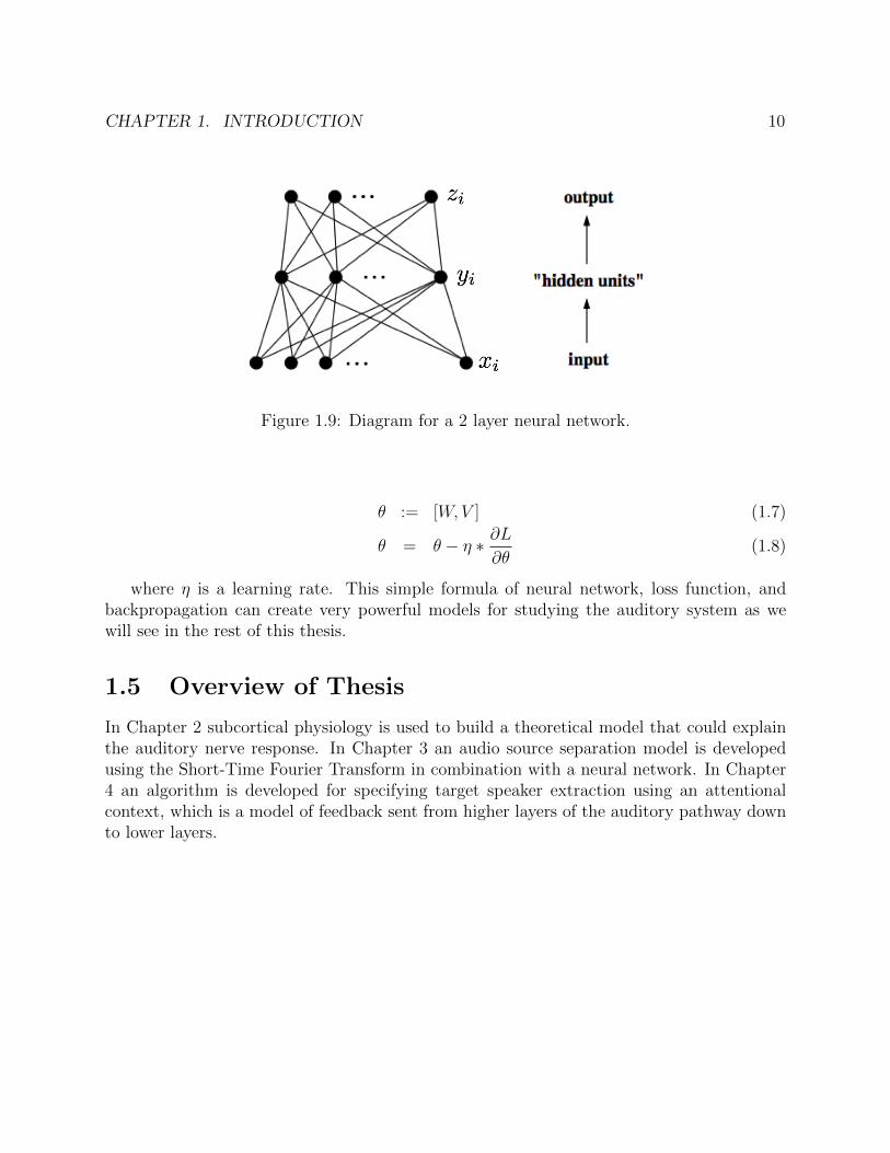
CHAPTER 1. INTRODUCTION 10
Figure 1.9: Diagram for a 2 layer neural network.
θ := [W,V ] (1.7)
θ = θ − η ∗ ∂L∂θ
(1.8)
where η is a learning rate. This simple formula of neural network, loss function, andbackpropagation can create very powerful models for studying the auditory system as wewill see in the rest of this thesis.
1.5 Overview of Thesis
In Chapter 2 subcortical physiology is used to build a theoretical model that could explainthe auditory nerve response. In Chapter 3 an audio source separation model is developedusing the Short-Time Fourier Transform in combination with a neural network. In Chapter4 an algorithm is developed for specifying target speaker extraction using an attentionalcontext, which is a model of feedback sent from higher layers of the auditory pathway downto lower layers.
11
Chapter 2
Neural Representations of Sound
2.1 Abstract
The theoretical principles of efficient coding have been used to explain the center-surroundand gabor receptive fields of retinal ganglion cells and neurons of the primary visual cortex.In this chapter similar ideas are used to explain not only the receptive field properties ofthe auditory nerve fibers, but their neural response themselves. The neural response hasa number of interesting properties which have never been explained: highly distributed,a precise timing code, and an intensity code using multiple fibers. The seminal work of[61] provides the best correspondence between efficient coding and the gammatone receptivefields of the auditory system but does not explain the neural response. In this research Iwill outline a model to rectify these shortcomings. Our results indicate that with betteroptimization this method may bring insight into neural representation of sound.
2.2 Introduction
One of the goals of theoretical neuroscience is to provide concise theories for how neuronsprocess information. By having a concise theory we can show that a large body of experi-mental results follows from a few intuitive ideas. Ideally, these theories are falsifiable, theycan be implemented and their results can be compared with experimental data. This al-lows us to iteratively improve our theories in order to understand the nature of the brainscomputation. In my project I would like to build such a theory - I will build a theory ofwhy encoding sound in the temporally precise firing patterns of the auditory nerve fiber isoptimal from an efficient coding perspective.
I first explain the efficient coding principle and how it has been used to provide a concisetheory of early visual processing. I then cover how these theories have been used to explainthe early auditory system and reflect on their shortcomings. Next I provide an overviewof the physiological results on the early auditory system to make these shortcomings moreclear. I then outline two possible theoretical models of early auditory processing that will
CHAPTER 2. NEURAL REPRESENTATIONS OF SOUND 12
start to resolve these differences. Finally, I propose a method to optimize these models usingrecent advances in Binary Neural Networks [10].
2.3 Coding
Efficient Coding
Animals have evolved their eyes in order to process images in a way that balances biologicalconstraints with the optical performance that is required for their particular environment.This claim is supported by the rich and diverse set of eyes that have evolved across the animalkingdom which can be explained as an adaptation to specific environmental conditions [33].Therefore, a theoretical explanation of an animals eyes can be provided through the principlesof optics, biological constraints, and the environmental conditions. This idea applies to visualprocessing equally, a theoretical model of visual processing can be obtained using the naturalvisual environment, an animals biological constraints, and the principles of visual processing.This is then the principle of efficient coding - to represent sensory information accuratelywith the fewest physical and metabolic resources.
Redundancy Reduction / Data Compression
At its core efficient coding represents a trade-off, a need to preserve more information aboutthe stimulus versus the metabolic cost of representing more information. In order to op-timally satisfy this constraint, it is necessary to exploit the statistical structure containedin natural stimuli. Attneave [3] was the first to introduce this idea, that visual perceptionwas related to the statistics of natural images. But it was Barlow [6] who eventually for-malized these ideas into the principle of redundancy reduction which states that neuronsshould minimize their statistical dependences with one another. By minimizing this statis-tical dependence while encoding as much information as possible they formed an efficientcode.
The theory of redundancy reduction was used by Atick and Redlich [2] to explain thecenter-surround properties of retinal ganglion cells (RGCs). Given the redundancy reduc-tion hypothesis, they claimed that RGCs should have receptive fields which act to pairwisedecorrelate their responses:
< Ri, Rj > = δ(i− j) ∀i, j (2.1)
Where Ri describes the response of RGC i and the average is, importantly, over samplesof natural images. In the Fourier domain this means that the amplitude of their responsesshould be flat, or uniform, over frequency. Since it had been shown by Field [18] that naturalscenes posses a 1/f 2 power spectrum then the amplitude of the optimal receptive field inthe Fourier domain should simply rise linearly with spatial frequency. Taking the inverseFourier transform of this function results a center-surround receptive field. This result was
CHAPTER 2. NEURAL REPRESENTATIONS OF SOUND 13
monumental - it was a powerful example of how the retina exploited the statistics of naturalimages in order to efficiently encode it.
Robust Coding
While redundancy reduction is an important principle in sensory coding, it is insufficient tocompletely explain how early sensory neurons encode information [5]. Neurons have a finitecapacity which has been estimated to be around 1-2 bits per spike [7]. In order transmitinformation reliably with neurons that have a fixed capacity it is necessary to have someamount of redundancy, this is has been referred to by Doi et al. [13] as robust coding. Doiand Lewicki [12] created an auto-encoder model where the hidden units were put through agaussian channel to approximate the limited capacity of neurons. By using an overcompleterepresentation they were able to overcome the channel noise to arbitrary precision givenmore units. By imposing an additional structural constraint on the filters, the optimalfilters strongly matched the center-surround receptive field structure of regional cells. Thus,they were able to motivate the center-surround filters from a much more general framework.Later, Karklin and Simoncelli [28] used these ideas with a metabolic constraint on the neuronresponses to show the optimality of center-surround receptive fields from a yet more generalframework.
Sparse Coding
While redundancy reduction and robust coding are important principles for understandinghow the brain encodes information efficiently, the brain must do more than this - it mustconstruct a meaningful representations of sensory information. Horace Barlowe was famousfor proposing one theory to build these representations, termed the ”neuron doctrine ofperception”, which proposed that neurons exploit the statistics of natural stimuli in order tobuild sparse representations of it. More precisely, the sensory stimuli at any given momentshould be described by a small fraction of neurons, forming a sparse representation. Theseideas were formalized mathematically by Olshausen and Field [50] who formed a parameteric,linear, generative model for images with a sparse prior. When optimized the basis functionsclosely matched the oriented receptive fields of V1 neurons, i.e. gabor functions. This wasanother powerful result in the field of theoretical neuroscience, the theory of sparse codingin the cortex had been used to explain the oriented receptive fields of V1 neurons.
Auditory Models
Given the success of sparse coding in the visual domain it was natural to wonder if it couldexplain the receptive field properties of the auditory nerve fibers. Lewicki [39] used a relatedmodel, Independent Component Analysis (ICA), on segments of sound and found that thelearned filters closely resembled the gammatone filters often used to describe the receptive
CHAPTER 2. NEURAL REPRESENTATIONS OF SOUND 14
field of the auditory nerve fibers. The next breakthrough came from Smith and Lewicki [61]where a convolutional sparse coding model was used to form a generative model of sound:
x(t) =∑i
bi(t) ? Si(t)
E =1
2||x(t)− x(t)||2
where bi(t) represents a scalar coefficient at time t, ? indicates convolution, and Si is atemporal kernel.
The optimization of this model consisted of iterating on the following two steps:
• Matching Pursuit - Find a sparse number of coefficients that best reconstruct the signal
• A gradient update of the kernel using these coefficients: Si = Si + η ∂E∂Si
The Matching Pursuit [46] algorithm itself consists of the following steps:
• Convolve the input signal with each basis function to get potential coefficent responsesfor the signal.
• Take the maximal response over coefficients and time. If this is less than a pre-definedthreshold then stop. If it is above, then remove this component from the input signaland iterate
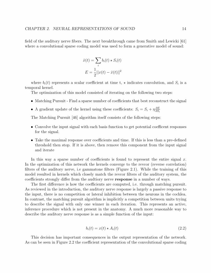
In this way a sparse number of coefficients is found to represent the entire signal x.In the optimization of this network the kernels converge to the revcor (reverse correlation)filters of the auditory nerve, i.e gammatone filters (Figure 2.1). While the training of thismodel resulted in kernels which closely match the revcor filters of the auditory system, thecoefficients strongly differ from the audtiory nerve response in a number of ways.
The first difference is how the coefficients are computed, i.e. through matching pursuit.As reviewed in the introduction, the auditory nerve response is largely a passive response tothe input, there is no competition or lateral inhibition between the neurons in the cochlea.In contrast, the matching pursuit algorithm is implicitly a competition between units tryingto describe the signal with only one winner in each iteration. This represents an active,inference procedure which is not present in the anatomy. A much more reasonable way todescribe the auditory nerve response is as a simple function of the input:
bi(t) = x(t) ? Ai(t) (2.2)
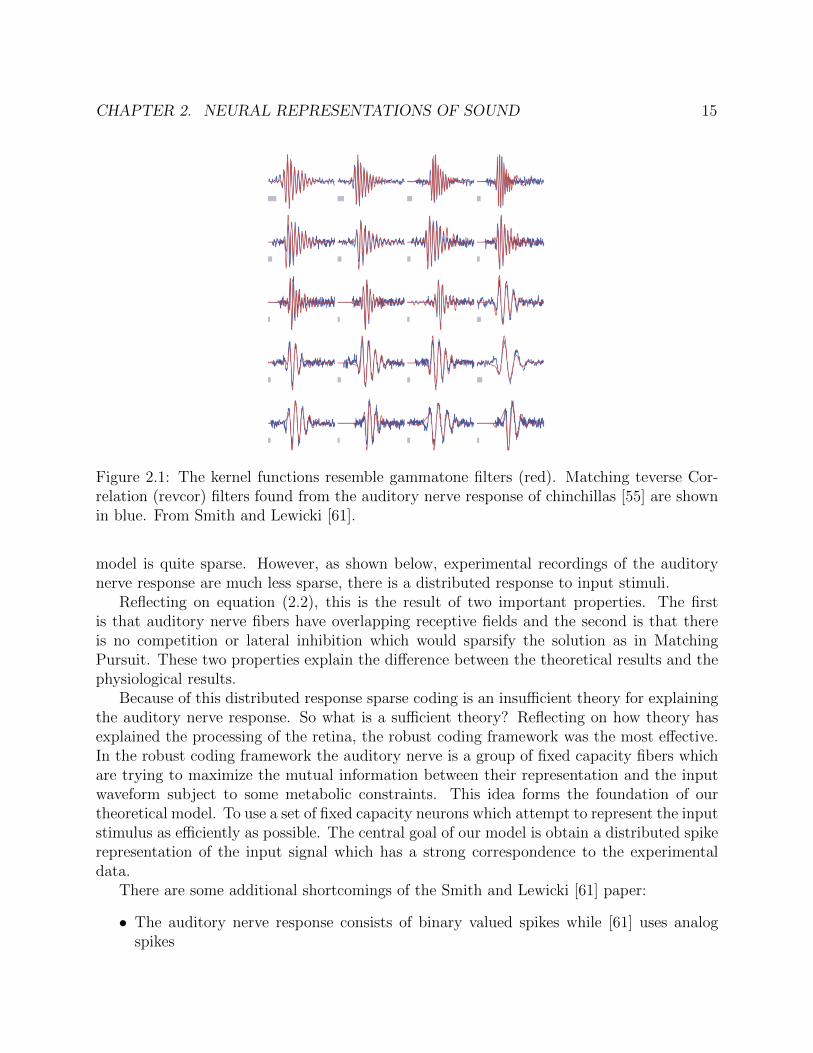
This decision has important consequences in the output representation of the network.As can be seen in Figure 2.2 the coefficient representation of the convolutional sparse coding
CHAPTER 2. NEURAL REPRESENTATIONS OF SOUND 15
Figure 2.1: The kernel functions resemble gammatone filters (red). Matching teverse Cor-relation (revcor) filters found from the auditory nerve response of chinchillas [55] are shownin blue. From Smith and Lewicki [61].
model is quite sparse. However, as shown below, experimental recordings of the auditorynerve response are much less sparse, there is a distributed response to input stimuli.
Reflecting on equation (2.2), this is the result of two important properties. The firstis that auditory nerve fibers have overlapping receptive fields and the second is that thereis no competition or lateral inhibition which would sparsify the solution as in MatchingPursuit. These two properties explain the difference between the theoretical results and thephysiological results.
Because of this distributed response sparse coding is an insufficient theory for explainingthe auditory nerve response. So what is a sufficient theory? Reflecting on how theory hasexplained the processing of the retina, the robust coding framework was the most effective.In the robust coding framework the auditory nerve is a group of fixed capacity fibers whichare trying to maximize the mutual information between their representation and the inputwaveform subject to some metabolic constraints. This idea forms the foundation of ourtheoretical model. To use a set of fixed capacity neurons which attempt to represent the inputstimulus as efficiently as possible. The central goal of our model is obtain a distributed spikerepresentation of the input signal which has a strong correspondence to the experimentaldata.
There are some additional shortcomings of the Smith and Lewicki [61] paper:
• The auditory nerve response consists of binary valued spikes while [61] uses analogspikes
CHAPTER 2. NEURAL REPRESENTATIONS OF SOUND 16
Figure 2.2: A spectrogram-like representation of the input stimulus using the optimal kernelsand coefficients. The kernels are ordered vertically by their center frequency. Colors simplydenote different kernels in this diagram. From [61].
• The auditory nerve response is known to have an important phase structure, wherethe timing of the spikes is strongly correlated with the peak of a periodic input. Themodel in [61] does not replicate this phase structure.
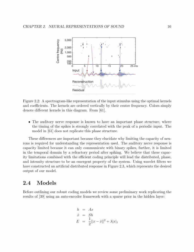
These differences are important because they elucidate why limiting the capacity of neu-rons is required for understanding the representation used. The auditory nerve response iscapacity limited because it can only communicate with binary spikes, further, it is limitedin the temporal domain by a refractory period after spiking. We believe that these capac-ity limitations combined with the efficient coding principle will lead the distributed, phase,and intensity structure to be an emergent property of the system. Using wavelet filters wehave constructed an artificial distributed response in Figure 2.3, which represents the desiredoutput of our model.
2.4 Models
Before outlining our robust coding models we review some preliminary work replicating theresults of [39] using an auto-encoder framework with a sparse prior in the hidden layer:
h = Ax
x = Sh
E =1
2||x− x||2 + λ|x|1
CHAPTER 2. NEURAL REPRESENTATIONS OF SOUND 17
Figure 2.3: Bottom - A spectrogram-like representation of speech from the GRID SpeechCorpus using wavelets (similar to gammatone filters) with overlapping receptive fields. Top- An artificial spike based representation using these filters. Note that the sound stimulus isrepresented in a highly distributed way, there are 5 artificial fibers firing in response to thefundamental frequency contained in the stimulus.
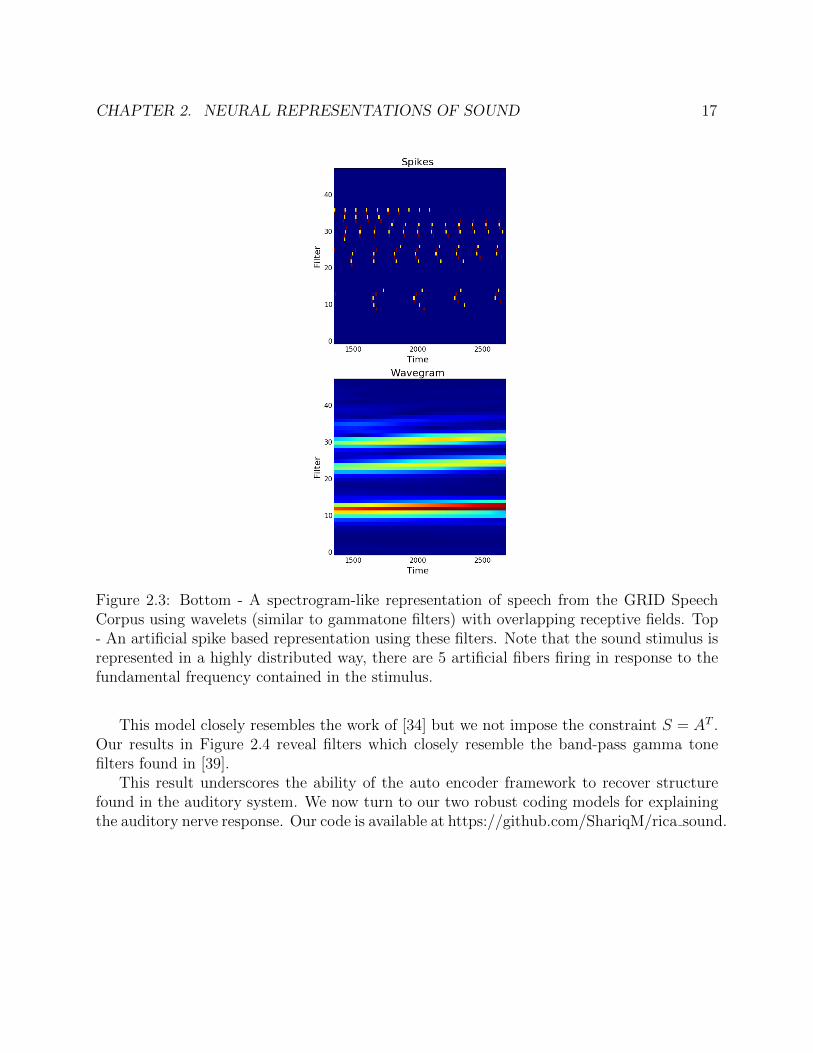
This model closely resembles the work of [34] but we not impose the constraint S = AT .Our results in Figure 2.4 reveal filters which closely resemble the band-pass gamma tonefilters found in [39].
This result underscores the ability of the auto encoder framework to recover structurefound in the auditory system. We now turn to our two robust coding models for explainingthe auditory nerve response. Our code is available at https://github.com/ShariqM/rica sound.
CHAPTER 2. NEURAL REPRESENTATIONS OF SOUND 18
Figure 2.4: Subset of basis functions learned in Model 1. All basis functions can be viewedhere: http://i.imgur.com/uUyBgV7.png
Model 1 - Convolutional AutoEncoder
The first model is a convolutional auto encoder where the hidden layer is subjected to noisein order to limit the capacity of neurons as in [13]:
bi(t) = x(t) ? Ai(t) + ni(t)
x(t) =∑i
bi(t) ? Si(t)
E =1
2
∑t
||x(t)− x(t)||2 + λ|b(t)|1
ni(t)iid∼ N (0, σ2
n)
We additionally impose a metabolic cost on b, instead of the structural constraint on A,as in [12]. A similar constraint was used in [28]. The goal of this model is to show gammatone filters can emerge from a simple capacity constraint rather than a sparsity constraint.
Model 2 - Convolutional LIF AutoEncoder
While the previous model would show how the gammatone filters can arise from a fixedcapacity constraint the noise model is not realistic. The reason the auditory nerve responseis limited in capacity is because it communicates using binary spikes at intervals of at least∼ 1ms due to the refractory period. Thus, the real question we want to answer is - Whatis the best way to encode the time-varying signal of sound into a spike-based code usingonly 30,000 nerve fibers, as in the human auditory system. To answer this question welimit the capacity of the hidden layer by using a leaky-integrate-and-fire (LIF) [15] model
CHAPTER 2. NEURAL REPRESENTATIONS OF SOUND 19
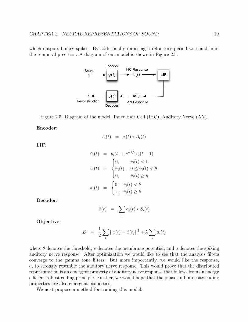
which outputs binary spikes. By additionally imposing a refractory period we could limitthe temporal precision. A diagram of our model is shown in Figure 2.5.
Figure 2.5: Diagram of the model. Inner Hair Cell (IHC). Auditory Nerve (AN).
Encoder:
bi(t) = x(t) ? Ai(t)
LIF:
vi(t) = bi(t) + e−1/τvi(t− 1)
vi(t) =
0, vi(t) < 0
vi(t), 0 ≤ vi(t) < θ
0, vi(t) ≥ θ
ai(t) =
{0, vi(t) < θ
1, vi(t) ≥ θ
Decoder:
x(t) =∑i
ai(t) ? Si(t)
Objective:
E =1
2
∑t
||x(t)− x(t)||2 + λ∑i
ai(t)
where θ denotes the threshold, v denotes the membrane potential, and a denotes the spikingauditory nerve response. After optimization we would like to see that the analysis filtersconverge to the gamma tone filters. But more importantly, we would like the response,a, to strongly resemble the auditory nerve response. This would prove that the distributedrepresentation is an emergent property of auditory nerve response that follows from an energyefficient robust coding principle. Further, we would hope that the phase and intensity codingproperties are also emergent properties.
We next propose a method for training this model.
CHAPTER 2. NEURAL REPRESENTATIONS OF SOUND 20
2.5 Training
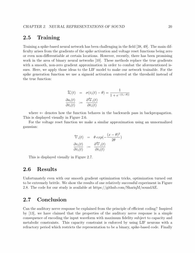
Training a spike-based neural network has been challenging in the field [38, 49]. The main dif-ficulty arises from the gradients of the spike activation and voltage reset functions being zeroor even non-differentiable at certain locations. However, recently, there has been promisingwork in the area of binary neural networks [10]. These methods replace the true gradientswith a smooth, non-zero gradient approximation in order to combat the aforementioned is-sues. Here, we apply those ideas to the LIF model to make our network trainable. For thespike generation function we use a sigmoid activation centered at the threshold instead ofthe true function:
←−ai (t) = σ(vi(t)− θ) =1
1 + e−(vi−θ))
∂ai(t)
∂vi(t):=
∂←−a i(t)
∂vi(t)
where ←− denotes how the function behaves in the backwards pass in backpropagation.This is displayed visually in Figure 2.6.
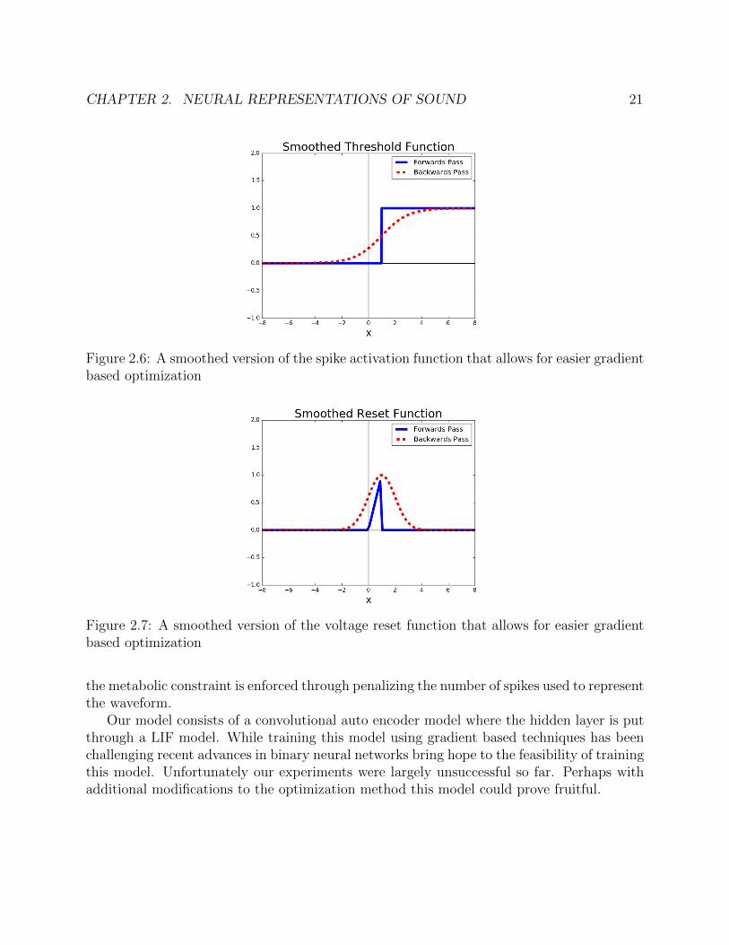
For the voltage reset function we make a similar approximation using an unnormalizedgaussian:
←−v i(t) = θ exp(−(x− θ)2
2θ)
∂vi(t)
∂vi(t):=
∂←−v i(t)
∂vi(t)
This is displayed visually in Figure 2.7.
2.6 Results
Unfortunately even with our smooth gradient optimization tricks, optimization turned outto be extremely brittle. We show the results of one relatively successful experiment in Figure2.8. The code for our study is available at https://github.com/ShariqM/soundAE.
2.7 Conclusion
Can the auditory nerve response be explained from the principle of efficient coding? Inspiredby [13], we have claimed that the properties of the auditory nerve response is a simpleconsequence of encoding the input waveform with maximum fidelity subject to capacity andmetabolic constraints. This capacity constraint is enforced by using LIF neurons with arefractory period which restricts the representation to be a binary, spike-based code. Finally
CHAPTER 2. NEURAL REPRESENTATIONS OF SOUND 21
Figure 2.6: A smoothed version of the spike activation function that allows for easier gradientbased optimization
Figure 2.7: A smoothed version of the voltage reset function that allows for easier gradientbased optimization
the metabolic constraint is enforced through penalizing the number of spikes used to representthe waveform.
Our model consists of a convolutional auto encoder model where the hidden layer is putthrough a LIF model. While training this model using gradient based techniques has beenchallenging recent advances in binary neural networks bring hope to the feasibility of trainingthis model. Unfortunately our experiments were largely unsuccessful so far. Perhaps withadditional modifications to the optimization method this model could prove fruitful.
CHAPTER 2. NEURAL REPRESENTATIONS OF SOUND 22
Figure 2.8: Computational experimental results with our model. Time is on the x-axis.This model has four neurons which correspond to the colors in the right column. Thereconstruction of the target input is shown in the left column.
23
Chapter 3
Robust Audio Source Separation
3.1 Abstract
In this chapter a cochlea-like representation, the spectrogram, is used to study audio sourceseparation, which is a major component of auditory scene analysis. This is joint work withmy colleague Brian Cheung. Recent work has shown that recurrent neural networks canbe trained to separate individual speakers in a sound mixture with high fidelity. Here weexplore convolutional neural network models as an alternative and show that they achievecompetitive results with an order of magnitude fewer parameters on standard benchmarks.We extend these benchmarks and compare the robustness of these different approachesto generalize under three new test conditions: longer time sequences, intermittent noise,and datasets outside the training domain. For the last condition, a new dataset is cre-ated, RealTalkLibri, to test source separation in real-world environments. This is used todemonstrate that the acoustics of the environment have significant impact on the over-all performance of neural network models, though our convolutional model shows supe-rior ability to generalize to new environments. The code for our study is available athttps://github.com/ShariqM/source separation.
3.2 Introduction
The sound waveform that arrives at our ears rarely comes from a single isolated source, butrather contains a complex mixture of multiple sound sources transformed in different waysby the acoustics of the environment. One of the central challenges of auditory scene analysisis to separate the components of this mixture so that individual sources may be recognized.Doing so generally requires some form of prior knowledge about the statistical structureof sound sources, such as common onset, co-modulation and correlation among harmoniccomponents [8, 11]. Our goal is to develop a model that can learn to exploit these forms ofstructure in the signal in order to robustly segment the time-frequency representation of asound waveform into its constituent sources (see Figure 3.1).
CHAPTER 3. ROBUST AUDIO SOURCE SEPARATION 24
Figure 3.1: Example of source separation using the spectrogram of two overlapped voices asinput. Left : Spectrogram of the mixture. Middle: Ground truth (oracle) source estimates(red and blue). Right : Source estimates using our convolutional model.
The problem of source separation has traditionally been approached within the frame-work of computational auditory scene analysis (CASA) [25]. These methods typically relyupon features such as gammatone filters in order to find a representation of the data that willallow for clustering methods to segment the individual speakers of the mixture. Recently,models which make these features learnable have been quite successful. Hershey et al. [23]introduced Deep Clustering (DPCL) which uses a Bi-directional Long short-term memory(BLSTM) [21] neural network to learn useful embeddings of time-frequency bins of a mix-ture. They formulate an objective function which encourages these embeddings to clusteraccording to their source so that K-means can be applied to partition the source signalsin the mixture. This model was further improved in the work of Isik et al. [26] and Chenet al. [9] which proposed simpler end-to-end models and achieved an impressive ∼10.5dBSignal-to-Distortion Ratio (SDR) in the source estimation signals.
In this work we develop an alternative model for source separation based on a dilatedconvolutional neural network architecture [73]. We show that it achieves state-of-the-artperformance with an order of magnitude fewer parameters and also generalizes better undernovel conditions and datasets. In addition, our convolutional approach only requires a smalland fixed amount of future information and can therefore operate in real-time.
An under- investigated aspect of deep learning algorithms is their ability to generalizeto new datasets. Models are usually trained, tested and compared against on the same datadistribution. In vision datasets, categories and tasks vary widely. In contrast, an auditorydataset provides a unique opportunity fix the task, i.e. to extract speech content, whilevarying the environment in which the data is recorded. In order to study the generalizationcapabilities of the models, we test them with inputs containing very long time sequences,intermittent noise, and mixtures collected under different recording conditions as in ourRealTalkLibri dataset.
Success in these more challenging domains is critical for progress to continue in robustsource separation, where the eventual goal is to be able to separate sources regardless ofspeaker identities, recording devices, and acoustical environments. Figure 3.2 shows threeexamples of how these factors can affect the spectrogram of the recorded waveform. Trainingmodels which can generalize to the space of these deformations is challenging. In vision andmachine learning, this issue is usually referred to as dataset bias [64, 65, 14] where models
CHAPTER 3. ROBUST AUDIO SOURCE SEPARATION 25
perform well on the training dataset but fail to generalize to new datasets. In recent yearsthe main approach to tackling this issue has been through data augmentation. In the speechcommunity, simulators for different acoustical environments [4, 31] have been leveraged tocreate more data. Recently, Variational Auto-Encoders [30] have begun to be used [24]. Invision and machine learning, Adversarial Network frameworks [20] have been used to improvegeneralization to different domains [65].
Figure 3.2: a: Original recording of a sin-gle female speaker from the LibriSpeechdataset; b,c,d : Recordings of the originalwaveform made with three different orienta-tions between computer speaker and record-ing device.
Figure 3.3: Recording setup diagram. Thespeakers were separated from the recordingdevice by different devices, each computerspeaker was responsible for playing a par-ticular source.
Here we show that the choice of model architecture alone can improve generalization.Our choice to use a convolutional architecture was inspired by the generalization power ofConvolutional Neural Networks (CNNs) [36, 32, 60] relative to fully connected networks. Wecompare the performance of our CNN model with the recurrent BLSTM models of previouswork and show that while both suffer when tested on new datasets the CNN model exhibitssuperior performance to the BLSTM.
3.3 Deep Attractor Framework
Notation: For a tensor T ∈ RA×B×C : T·,·,c ∈ RA×B is a matrix, and Ta,·,c ∈ RB is a vector,and Ta,b,c ∈ R is a scalar.
Embedding the mixed waveform
Chen et al. [9] propose a framework for single-channel speech separation. x ∈ Rτ is araw input signal of length τ and X ∈ RF×T is its spectrogram computed using the Short-
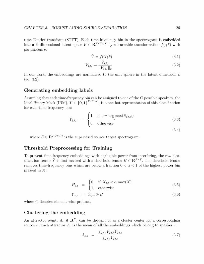
CHAPTER 3. ROBUST AUDIO SOURCE SEPARATION 26
time Fourier transform (STFT). Each time-frequency bin in the spectrogram is embeddedinto a K-dimensional latent space V ∈ RF×T×K by a learnable transformation f(·; θ) withparameters θ:
V = f(X; θ) (3.1)
Vf,t,· =Vf,t,·||Vf,t,·||2
(3.2)
In our work, the embeddings are normalized to the unit sphere in the latent dimension k(eq. 3.2).
Generating embedding labels
Assuming that each time-frequency bin can be assigned to one of the C possible speakers, theIdeal Binary Mask (IBM), Y ∈ {0,1}F×T×C , is a one-hot representation of this classificationfor each time-frequency bin:
Yf,t,c =
1, if c = arg maxc′
(Sf,t,c′)
0, otherwise(3.3)
(3.4)
where S ∈ RF×T×C is the supervised source target spectrogram.
Threshold Preprocessing for Training
To prevent time-frequency embeddings with negligible power from interfering, the raw clas-sification tensor Y is first masked with a threshold tensor H ∈ RF×T . The threshold tensorremoves time-frequency bins which are below a fraction 0 < α < 1 of the highest power binpresent in X:
Hf,t =
{0, if Xf,t < α max(X)
1, otherwise(3.5)
Y·,·,c = Y·,·,c �H (3.6)
where � denotes element-wise product.
Clustering the embedding
An attractor point, Ac ∈ RK , can be thought of as a cluster center for a correspondingsource c. Each attractor Ac is the mean of all the embeddings which belong to speaker c:
Ac,k =
∑f,t Vf,t,kYf,t,c∑
f,t Yf,t,c(3.7)

CHAPTER 3. ROBUST AUDIO SOURCE SEPARATION 27
During training the attractor points are calculated using the thresholded oracle mask,Y . In the absence of the oracle mask at test time, the attractor points are calculated usingK-means. Only the embeddings which pass the corresponding time-frequency bin thresholdare clustered.
Finally the mask is computed by taking the inner product of all embeddings with allattractors and applying a softmax:
Mf,t,c = softmaxc
(∑k
Ac,kVf,t,k
)(3.8)
S·,·,c = M·,·,c �X (3.9)
From this mask, we can compute source estimate spectrograms (3.9) which in turn can beconverted back to an audio waveform via the inverse STFT. We do not attempt to computethe phase of the source estimates. Instead, we use the phase of the mixture to compute theinverse STFT with the magnitude source estimate spectrogram S.
The loss function L is the mean-squared-error (MSE) of the source estimate spectrogramand the supervised source target spectrogram, S ∈ RF×T×C :
L =∑c
||S·,·,c − S·,·,c||2F (3.10)
where || · ||F denotes the Frobenius norm. See Figure 3.4 for an overview of our sourceseparation process.
Figure 3.4: Overview of the source separation process.
Network Architecture
A variety of neural network architectures are candidates to parameterize the embeddingfunction in Equation 3.1. Chen et al. [9] use a 4-layer Bi-Directional LSTM architecturewhich utilizes weight sharing across time, allowing it to process inputs of variable temporallength.
By contrast, convolutional neural networks are capable of sharing weights along boththe time and frequency axis. Recently convolutional neural networks have been shown to
CHAPTER 3. ROBUST AUDIO SOURCE SEPARATION 28
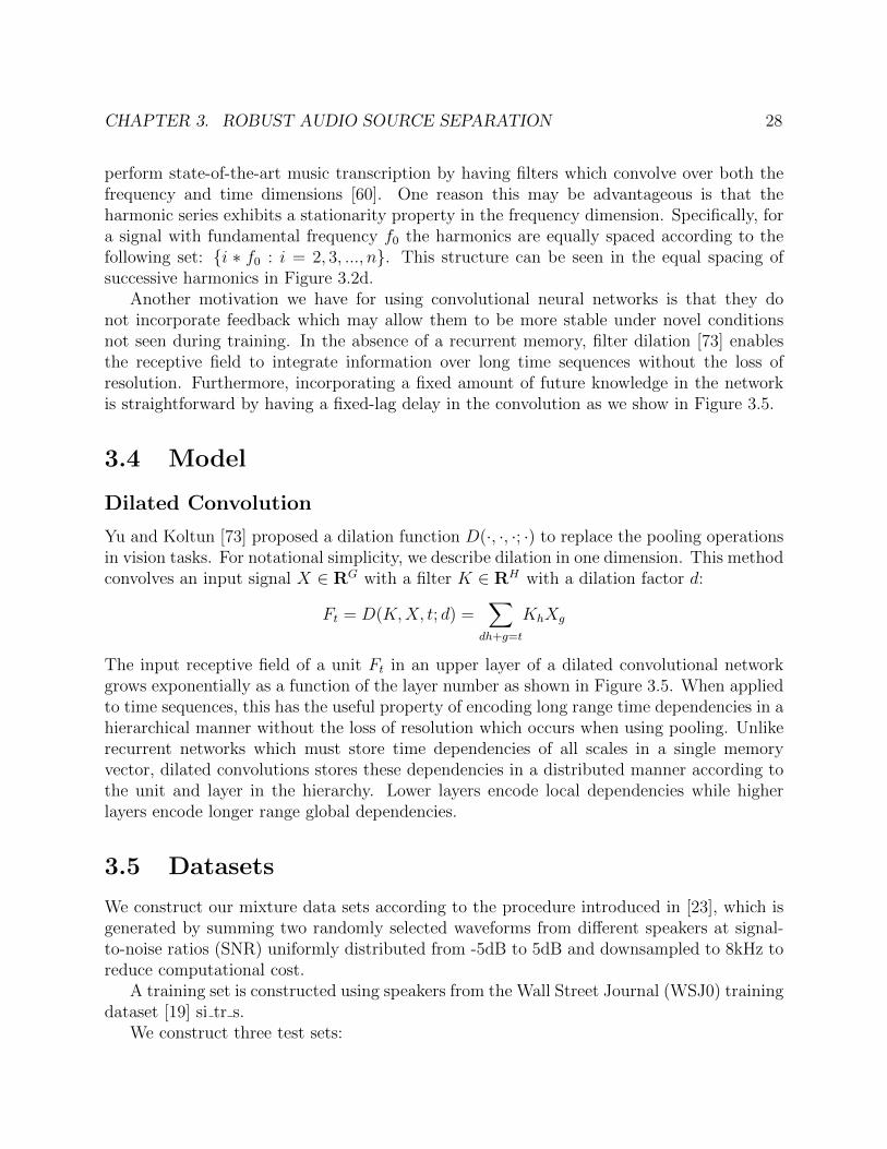
perform state-of-the-art music transcription by having filters which convolve over both thefrequency and time dimensions [60]. One reason this may be advantageous is that theharmonic series exhibits a stationarity property in the frequency dimension. Specifically, fora signal with fundamental frequency f0 the harmonics are equally spaced according to thefollowing set: {i ∗ f0 : i = 2, 3, ..., n}. This structure can be seen in the equal spacing ofsuccessive harmonics in Figure 3.2d.
Another motivation we have for using convolutional neural networks is that they donot incorporate feedback which may allow them to be more stable under novel conditionsnot seen during training. In the absence of a recurrent memory, filter dilation [73] enablesthe receptive field to integrate information over long time sequences without the loss ofresolution. Furthermore, incorporating a fixed amount of future knowledge in the networkis straightforward by having a fixed-lag delay in the convolution as we show in Figure 3.5.
3.4 Model
Dilated Convolution
Yu and Koltun [73] proposed a dilation function D(·, ·, ·; ·) to replace the pooling operationsin vision tasks. For notational simplicity, we describe dilation in one dimension. This methodconvolves an input signal X ∈ RG with a filter K ∈ RH with a dilation factor d:
Ft = D(K,X, t; d) =∑
dh+g=t
KhXg
The input receptive field of a unit Ft in an upper layer of a dilated convolutional networkgrows exponentially as a function of the layer number as shown in Figure 3.5. When appliedto time sequences, this has the useful property of encoding long range time dependencies in ahierarchical manner without the loss of resolution which occurs when using pooling. Unlikerecurrent networks which must store time dependencies of all scales in a single memoryvector, dilated convolutions stores these dependencies in a distributed manner according tothe unit and layer in the hierarchy. Lower layers encode local dependencies while higherlayers encode longer range global dependencies.
3.5 Datasets
We construct our mixture data sets according to the procedure introduced in [23], which isgenerated by summing two randomly selected waveforms from different speakers at signal-to-noise ratios (SNR) uniformly distributed from -5dB to 5dB and downsampled to 8kHz toreduce computational cost.
A training set is constructed using speakers from the Wall Street Journal (WSJ0) trainingdataset [19] si tr s.
We construct three test sets:
CHAPTER 3. ROBUST AUDIO SOURCE SEPARATION 29
Figure 3.5: One-dimensional, fixed-lag dilated convolutions used by our model with dilationfactors of 1, 2 and 4. The bottom row represents the input and each successive row is anotherlayer of convolution. This network has a fixed-lag of 4 timepoints before it can output adecision for the current input.
• WSJ0 : a test set is constructed identical to the test set introduced in [23] using 18unheard speakers from si dt 05 and si et 05.
• LibriSpeech: a test set is constructed using 40 unheard speakers from test-clean.
• RealTalkLibri : we generate more realistic mixture using the procedure described below.
RealTalkLibri Dataset
We are interested in collecting a speech mixture dataset with two properties:
1. Speech mixtures are deformed by the acoustics of the room.
2. Availability of ground truth for the source waveforms.
Unfortunately all audio datasets that have property (1) don’t have property (2) [31, 4].These datasets only provide the transcription. In order to fill this void and investigategeneralization we created a small test dataset with both these properties.
The RealTalkLibri (RTL) test dataset is created starting from the test-clean directoryof the open LibriSpeech dataset [53] which contains clean speech from 40 speakers. Wefirst downsampled all waveforms to 8kHz as before. Each mixture in the dataset is createdby sampling two random speakers from the test-clean partition of LibriSpeech, picking arandom waveform and start time for each, and playing the waveforms through two Logitechcomputer speakers for 12 seconds. The waveforms of the two speakers are played in separatechannels linked to a left and right computer speaker, separated from the microphone of the

CHAPTER 3. ROBUST AUDIO SOURCE SEPARATION 30
computer by different distances. The recordings are made with a sample rate of 8kHz usinga 2013 MacBook Pro. Figure 3.3 is a diagram of our data collection process.
In order to obtain ground truth of the individual speaker waveforms each of the waveformsis played twice, once in isolation and once simultaneously with the other speaker. The firstrecording represents the ground truth and the second one is for the mixture. To verifythe quality of the ground truth recordings, we constructed an ideal binary mask Y whichperforms about as well on the previous simulated datasets, see the Oracle performance inFigure 3.9. The RealTalkLibri data set is made up of two recording sessions which eachyielded 4.5 hours of data, giving us a total of 9 hours of test data. The dataset is madefreely available at https://www.dropbox.com/s/4pscejhkqdr8xrk/rtl.tar.gz?dl=0.
3.6 Experiments
Experimental Setup
We evaluate the models on a single-channel simultaneous speech separation task. The mix-ture waveforms are transformed into a time-frequency representation using the Short-timeFourier Transform (STFT) and the log-magnitude features, X, are served as input to themodel. The STFT is computed with 32ms window length, 8ms hop size, and the Hannwindow. We use SciPy to compute the STFT and TensorFlow to build our neural networks.
We report our results using the signal-to-distortion ratio (SDR) metric introduced in [67]as a blind audio source separation (BSS) metric. We compute our results using version 3of the Matlab bsseval toolbox [17]. A python implementation of this code is also availableonline [54] 1.
Our network consists of 13 dilated convolutional layers [73] made up of two stacks, eachstack having its dilation factor double each layer. Batch Normalization is applied to eachlayer and residual connections [22] are used at every other layer, see Table 3.1 for details.
Layer 1 2 3 4 5 6 7 8 9 10 11 12 13
Convolution 3x3 3x3 3x3 3x3 3x3 3x3 3x3 3x3 3x3 3x3 3x3 3x3 3x3
Dilation 1x1 2x2 4x4 8x8 16x16 32x32 1x1 2x2 4x4 8x8 16x16 32x32 1x1
Residual No Yes No Yes No Yes No Yes No Yes No Yes No
Channels 128 128 128 128 128 128 128 128 128 128 128 128 K
Table 3.1: Dilated Convolutional Network Architecture
We reimplement the DANet of [9] with a BLSTM architecture containing 4 layers and500 hidden units in both the forward and backward LSTM, for a total of 1000 hidden units.
1https://github.com/craffel/mir_eval/blob/master/mir_eval/separation.py
CHAPTER 3. ROBUST AUDIO SOURCE SEPARATION 31
Model WSJ0 Number ofSDR (dB) Parameters
DANet (BLSTM) 10.48 17 114 580DPCL* (BLSTM) 10.8 ?
Ours (CNN) 10.97 1 650 836Oracle 13.49 -
Table 3.2: SDR for two competitor models, our proposed convolutional model, and theOracle. Our model achieves the best results using significantly fewer parameters. Scoresaveraged over 3200 examples. *: SDR score is from [26] which is at an advantage due to asecond enhancement neural network after masking.
We replicated their training schedule using the RMSProp algorithm [63], a starting learningrate of 1e−3, and exponential decay with parameters: decay steps= 2000, decay rate= 0.95.
For evaluation we also use the max() function rather than the softmax() for computingthe mask in equation (3.8). We calculate an Oracle score using the Ideal Binary Mask (IBM),Y , using the ground truth source spectrograms (Eq. 3.4).
WSJ0 Evaluation
We begin by evaluating the models on the WSJ0 test dataset as in [9]. Our results are shownin Table 3.2. Our model achieves the best score using a factor of ten fewer parameters thanDANet. The DPCL score is taken from [26] which has a very similar architecture to DANetand therefore a similar number of parameters. Their model has one important differencehowever, a second neural network is used to enhance the source estimate spectrogram toachieve their result. Our model is still able to exceed its performance without this extraenhancement network. In addition, our model has a fixed window into the future whereasthe BLSTM models have access to the entire future. This indicates that a convolutionbased architecture is better at solving this source separation task with less information incomparison to a recurrent based architecture.
Embeddings
At test time the K-means must be employed because the labels Y are not available forcalculating the attractors (3.7). In order for the attractors to from a good proxy for theK-means algorithm we applied l2 normalization (Eq. 3.2) to the embeddings V . In Figure3.6 we visualize the embedding outputs of our model using PCA for a single mixture acrossT = 200 timepoints. Each embedding point corresponds to a single time-frequency bin inthe mixed input spectrogram. The embeddings are colored in this diagram according tothe oracle labelling, red for speaker 1 and blue for speaker 2. Notice that the network has
CHAPTER 3. ROBUST AUDIO SOURCE SEPARATION 32
learned to cluster the embeddings according to the speaker they belong too, i.e. there is ahigh density of red embeddings on the left and similarly for blue embeddings on the right.This structure allows K-means to easily find cluster centers that match the attractors usedat training time.
Figure 3.6: Embeddings for two speakers (red & blue) projected onto a 3-dimensional sub-space using PCA. The orange points correspond to time-frequency bins where the energywas below threshold (see 3.5). There are T × F = 200 × 129 = 25800 embedding points intotal.
Generalization Experiments
Length Generalization
In the first experiment we study how well these models work under time-sequences 25xlonger than they are trained on, i.e. T = 10000 (∼ 80s). Previous work [27] has indicatedthat because recurrent architectures incorporate feedback they can function unpredictablyfor sequence lengths beyond those seen during training. On the other hand, convolutionalnetwork architectures do not incorporate any feedback. This is advantageous for processingtime sequences of indefinite length because errors cannot accumulate over time. Since aconvolutional network is a stationary process in the convolved dimension, we hypothesizethis architecture will operate more robustly over sequence lengths much longer than thoseseen during training. Our results are shown in Figure 3.7a. Surprisingly, the results indicatethat the BLSTM is also able to generalize to sequences of significantly larger length, contraryto our expectations. We discuss possible explanations of this result in the next section. OurCNN model is able to maintain its performance across the long sequence as expected.
CHAPTER 3. ROBUST AUDIO SOURCE SEPARATION 33
Figure 3.7: Results of the length and noise generalization experiments. For both plots, weplot the SDR starting at the time specified by the x-axis up until 400 time points (∼ 3s)later. Both the BLSTM and CNN are (a) able to operate over very long time sequences and(b) recover from intermittent noise. See Figure 3.8 for the spectrogram in b).
Figure 3.8: Source separation spectrogram for the noise generalization experiment.
Noise Generalization
In the second experiment we are interested in how the models respond to small bursts ofinput data far outside of the training distribution. We believe the BLSTM model mightbecome unstable as a result of such inputs because its recurrent structure makes it possiblefor the noise to affect its hidden state indefinitely. We took sequences of length T = 1200(∼ 9s) and inserted white noise for 0.25s in the middle of the mixture to disrupt the modelsprocess. Our results are shown in Figure 3.7b. Again, contrary to our belief the BLSTM isvery resilient to this noise, the model quickly recovers after the noise passes (last data point).One possible explanation is that the BLSTM is only integrating information over short timescales and therefore “forgets” about previous input data after a short number of time steps.We believe this is because when we construct the input for our models we randomly samplea starting time for each waveform. This may force the BLSTM to learn a stationary function
CHAPTER 3. ROBUST AUDIO SOURCE SEPARATION 34
Figure 3.9: Results of the models tested on WSJ0 simulated mixtures, LibriSpeech simulatedmixtures, and our RealTalkLibri (RTL) dataset. Our model performs the best on WSJ0,generalizes better to LibriSpeech, but fails alongside the BLSTM at generalizing to the realmixtures of RTL. All models are trained on WSJ0. *: Model has a second neural networkto enhance the source estimate spectrogram and is therefore at an advantage. The modelwasn’t available online for testing against LibriSpeech or RTL.
since it must be able to separate the mixture with or without information from the past inits hidden state.
Data Generalization
In the final experiment we are interested in how well the models generalize to data progres-sively farther from the training distribution. We trained all the models on the WSJ0 trainingset and then tested on the WSJ0 test set, the LibriSpeech test set, and RealTalkLibri testset. Our results are shown in Figure 3.9. Our model generalizes quite well from the WSJ0dataset to the LibriSpeech dataset, only losing 1.8dB of performance. Unfortunately it de-grades substantially when using the RTL dataset. However, our model still outperforms theDANet model on all datasets.
In Figure 3.10 we visualize the mistakes our network makes under the RealTalkLibridataset. The first example indicates that the model does not have a strong enough bias tothe harmonic structure contained in speech, it classifies the frequencies of the fundamental toa different speaker than the harmonic frequencies of that fundamental. The second exampleindicates that the model also has issues with temporal continuity, the speaker identity ofparticular frequency bins varies sporadically across time. This indicates that there is stillroom to improve generalization in these models by modifying model architecture and addingregularization.
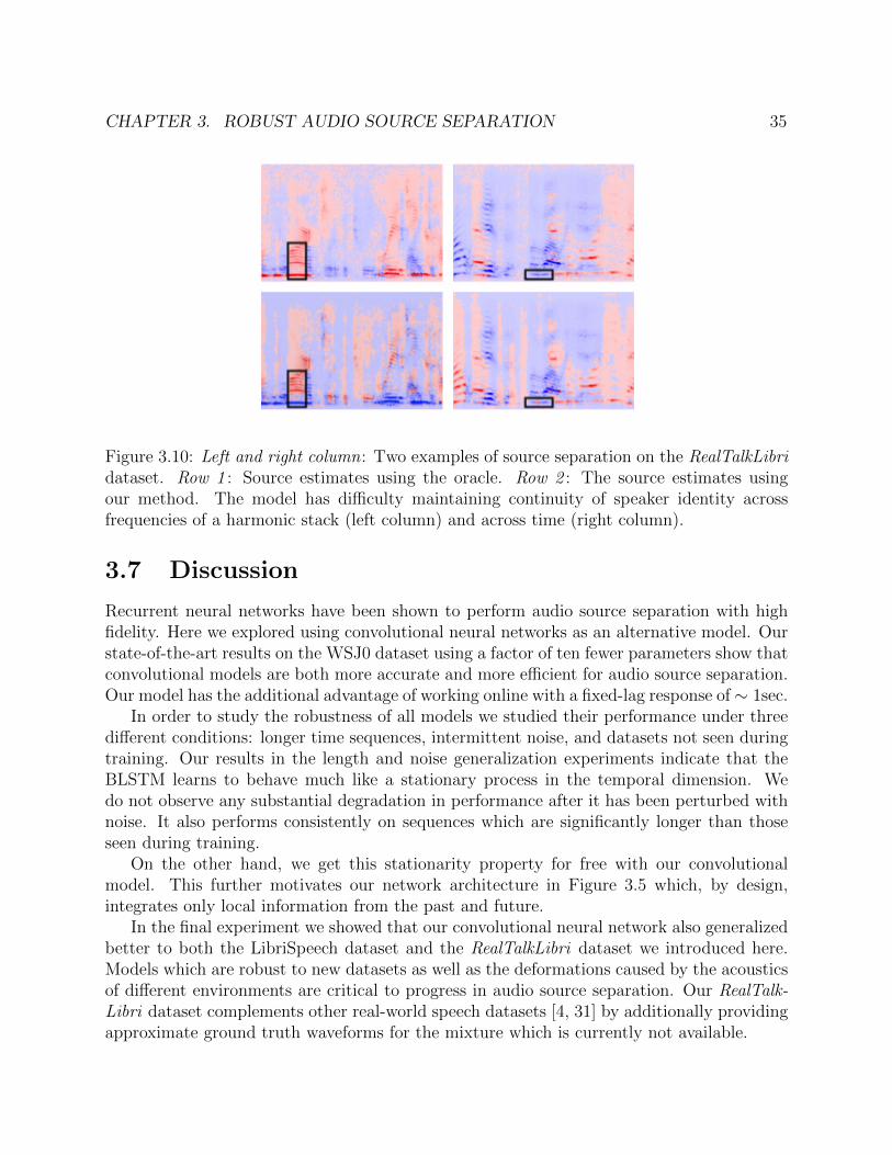
CHAPTER 3. ROBUST AUDIO SOURCE SEPARATION 35
Figure 3.10: Left and right column: Two examples of source separation on the RealTalkLibridataset. Row 1 : Source estimates using the oracle. Row 2 : The source estimates usingour method. The model has difficulty maintaining continuity of speaker identity acrossfrequencies of a harmonic stack (left column) and across time (right column).
3.7 Discussion
Recurrent neural networks have been shown to perform audio source separation with highfidelity. Here we explored using convolutional neural networks as an alternative model. Ourstate-of-the-art results on the WSJ0 dataset using a factor of ten fewer parameters show thatconvolutional models are both more accurate and more efficient for audio source separation.Our model has the additional advantage of working online with a fixed-lag response of ∼ 1sec.
In order to study the robustness of all models we studied their performance under threedifferent conditions: longer time sequences, intermittent noise, and datasets not seen duringtraining. Our results in the length and noise generalization experiments indicate that theBLSTM learns to behave much like a stationary process in the temporal dimension. Wedo not observe any substantial degradation in performance after it has been perturbed withnoise. It also performs consistently on sequences which are significantly longer than thoseseen during training.
On the other hand, we get this stationarity property for free with our convolutionalmodel. This further motivates our network architecture in Figure 3.5 which, by design,integrates only local information from the past and future.
In the final experiment we showed that our convolutional neural network also generalizedbetter to both the LibriSpeech dataset and the RealTalkLibri dataset we introduced here.Models which are robust to new datasets as well as the deformations caused by the acousticsof different environments are critical to progress in audio source separation. Our RealTalk-Libri dataset complements other real-world speech datasets [4, 31] by additionally providingapproximate ground truth waveforms for the mixture which is currently not available.
CHAPTER 3. ROBUST AUDIO SOURCE SEPARATION 36
Looking forward, we aim to improve the generalization ability of the models on examplessuch as those shown in Figure 3.10 by introducing a training set for RealTalkLibri, developingmore robust model architectures, introducing regularizers for the structure of speech, andcreating powerful data augmentation tools. We also believe models which can operate underan unknown number of sources is of utmost importance to the field of audio source separation.
37
Chapter 4
Auditory Attention
4.1 Abstract
In this chapter algorithms for focusing on a specific speaker are investigated, rather thanextracting all the sources in the mixture. Recent work has shown that neural networks canperform speaker separation with high fidelity. Most methods have been speaker independentbut recently research into methods for speaker biased output have been popular. The mainidea is to bias the output of a neural network by feeding it an attentional context, a targetspeaker embedding that is computed from a target voice snippet. In all previous methods thebias has been for a single speaker which makes the methods inferior to speaker independentmethods, which can extract multiple speakers simultaneously. In this chapter a novel idea toperform multi-speaker biased extraction is developed by casting the multi-speaker embeddingas a simple superposition of the individual speaker embeddings. This allows our attentionmodels to extract an arbitrary subset of target speakers from a mixture of an unknownnumber of sources, making the method superior to speaker independent methods, whichmust know the number of sources in the input. The results show multi-speaker-embeddingsperform only slightly worse than single-speaker-embedding demonstrating the effectivenessof the superposition method. Finally, a new method to compute speaker embeddings, calledinference-embeddings, is developed which can use substantially more voice data than thevoice snippet method of previous work.
4.2 Introduction
While our conscious experience of sound consists of a number of distinct, separate, sound-producing events, the raw auditory stimuli received contains a mixture of them. One ofthe goals of auditory scene analysis is to separate this complex mixture into the distinctsources that make it [8]. However, this ability super human, humans cannot always focustheir attention on every distinct source, and instead must direct their attention to a smallset of sources which are behaviourally relevant. This attentional mechanism is thought to be
CHAPTER 4. AUDITORY ATTENTION 38
mediated by top down attention, where high level signals, which correspond to the sourcesof interest, are fed into lower levels of computation in order to extract the relevant sources[29]. The goal is to develop neural network models which can extract the sources of interestusing these high level signals.
Deep learning models of speech separation are not typically viewed from the perspectiveof top-down attention but there are strong connections in the speaker-biased separationliterature. Deep learning based speech separation systems are often classified into two groups:speaker-independent and speaker-biased speech separation. In the first approach the modelattempts to separate the sound mixture into all of it’s constituent sources at once. Modelsthat follow this approach project components of the sound into a high dimensional spacewhere K-means can be applied to extract the K sources in the mixture. Using deep learning,these methods have been shown to be extremely effective, e.g. deep clustering (DPCL) [22],attractor network [9], etc. [72, 48]. However, a major drawback of this approach is that thenumber of sources in the mixture, K, must be known before hand otherwise the algorithmfails.
By contrast, the speaker-biased approaches only extract a target speaker, while all otherspeakers are considered interference. An attention context vector must be supplied to in-dicate which speaker is of interest to the network. The advantage of this method is that,in theory, this method should be agnostic to the number of inputs in the mixture, which isdemonstrated in this chapter. Again using deep learning, this approach has been shown to bequite effective [68, 74, 71] Currently, there are two disadvantages of this method when com-pared to speaker-independent separation, multiple sources cannot be extracted, and priorknowledge of the speakers must be supplied. More succinctly here are the advantages anddisadvantages of these two approaches:
Speaker-Independent
+ Requires no prior knowledge of speakers
+ Ability to extract an arbitrary number of sources
- Requires the number of sources in the mixture to be known
Speaker-Biased
- Requires prior knowledge of speakers
- Can only extract a single source
+ Agnostic to the number of sources in the input
But are these current disadvantages inherent to the algorithm? We believe both can beresolved as actual advantages making the speaker-biased approach superior in all respects.In this chapter the focus is on how multiple sources can be extracted. Ideas for how the
CHAPTER 4. AUDITORY ATTENTION 39
inference-embeddings technique could be used to solve the requirement of prior knowledgeis explored after.
One of the motivations for solving the multiple source issue is to replicate the humanability to focus attention on a subset of speakers in an environment with many speakers.For example, in the cocktail party problem. The final experiment of this chapter replicatessuch a scenario.
For speaker-biased methods the prior knowledge of speakers comes from a snippet ofreference audio from the target speaker. An additional network computes an embeddingfrom this snippet and hands it to the separation network [71]. This method works wellbut is limited to using a short piece of reference audio, on the order of 10 seconds. In thischapter, an inference-embeddings method is described which can use much more data.
We make the following contributions:
• Extend speaker-biased models to handle the extraction of multiple speakers using em-bedding superpositions.
• Develop a new method to compute embeddings, termed inference-embeddings, whichhas the advantage of utilizing an arbitrary amount of data rather than a short snippetof reference audio.
• Demonstrate the strongest advantage of speaker-biased models, to be agnostic to thenumber of sources in the input, using our superposition method.
4.3 Multi-Speaker Extraction
Task Description
We propose a single-channel multi-speaker biased speech separation task. The task is toextract multiple target speakers’ voices from a mixed speech waveform. Two sets of speakersare analyzed, known speakers, and new speakers. Known speakers represent speakers ouralgorithms has substantial data on and help train the baseline model. New speakers representspeakers our algorithms have minimal data on and are challenged to learn to separate wellby relying on fine-tuning the baseline model.
Multi-Speaker Extraction Framework
Setup
Notation: For a tensor T ∈ RA×B×C : T·,·,c ∈ RA×B is a matrix, Ta,·,c ∈ RB is a vector, andTa,b,c ∈ R is a scalar.
Let Nk be the number of known speakers, Nn the number of new speakers that must belearned after the initial training on the Nk speakers, and N = Nk +Nn be the total numberof speakers.
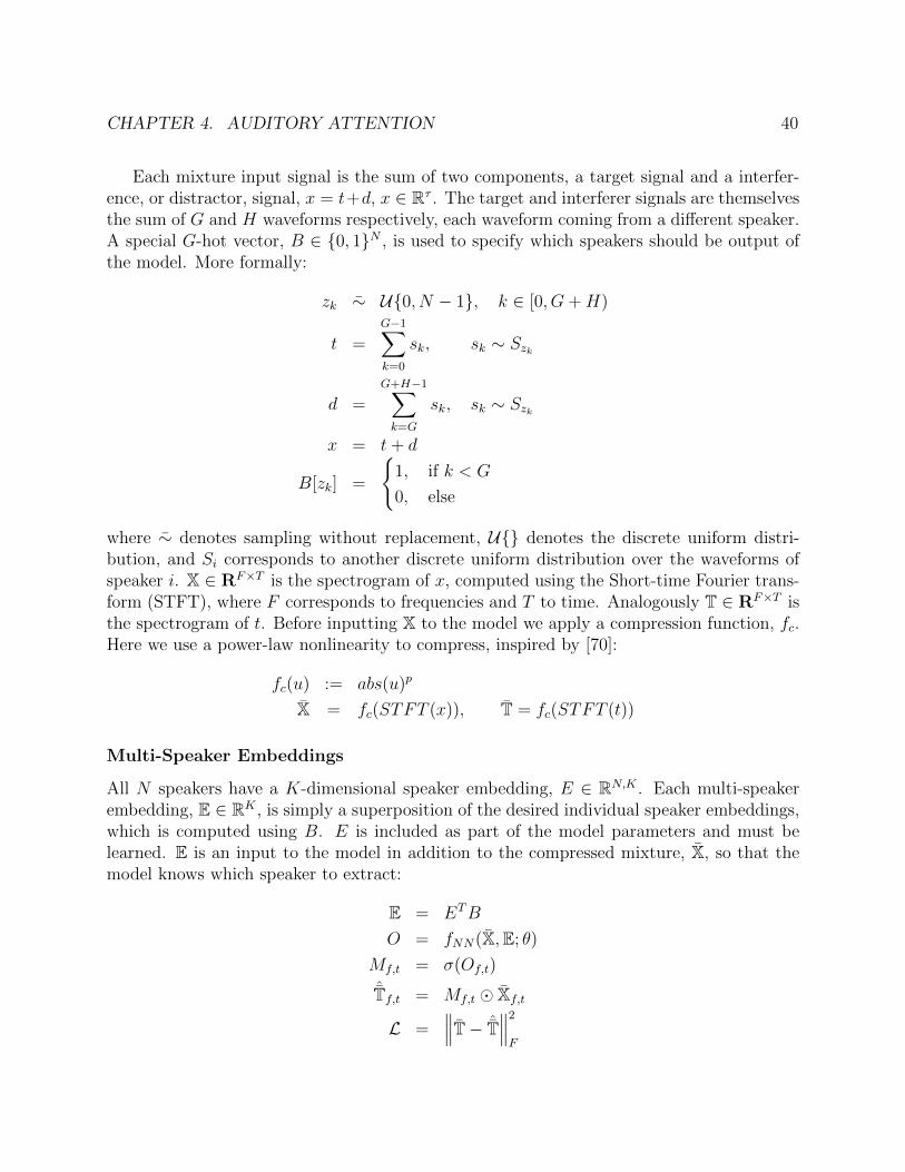
CHAPTER 4. AUDITORY ATTENTION 40
Each mixture input signal is the sum of two components, a target signal and a interfer-ence, or distractor, signal, x = t+d, x ∈ Rτ . The target and interferer signals are themselvesthe sum of G and H waveforms respectively, each waveform coming from a different speaker.A special G-hot vector, B ∈ {0, 1}N , is used to specify which speakers should be output ofthe model. More formally:
zk ∼ U{0, N − 1}, k ∈ [0, G+H)
t =G−1∑k=0
sk, sk ∼ Szk
d =G+H−1∑k=G
sk, sk ∼ Szk
x = t+ d
B[zk] =
{1, if k < G
0, else
where ∼ denotes sampling without replacement, U{} denotes the discrete uniform distri-bution, and Si corresponds to another discrete uniform distribution over the waveforms ofspeaker i. X ∈ RF×T is the spectrogram of x, computed using the Short-time Fourier trans-form (STFT), where F corresponds to frequencies and T to time. Analogously T ∈ RF×T isthe spectrogram of t. Before inputting X to the model we apply a compression function, fc.Here we use a power-law nonlinearity to compress, inspired by [70]:
fc(u) := abs(u)p
X = fc(STFT (x)), T = fc(STFT (t))
Multi-Speaker Embeddings
All N speakers have a K-dimensional speaker embedding, E ∈ RN,K . Each multi-speakerembedding, E ∈ RK , is simply a superposition of the desired individual speaker embeddings,which is computed using B. E is included as part of the model parameters and must belearned. E is an input to the model in addition to the compressed mixture, X, so that themodel knows which speaker to extract:
E = ETB
O = fNN(X,E; θ)
Mf,t = σ(Of,t)
ˆTf,t = Mf,t � Xf,t
L =∥∥∥T− ˆT
∥∥∥2
F
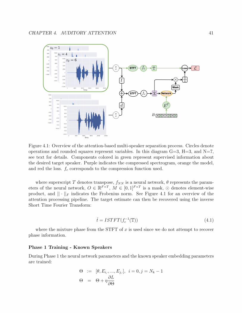
CHAPTER 4. AUDITORY ATTENTION 41
Figure 4.1: Overview of the attention-based multi-speaker separation process. Circles denoteoperations and rounded squares represent variables. In this diagram G=3, H=3, and N=7,see text for details. Components colored in green represent supervised information aboutthe desired target speaker. Purple indicates the compressed spectrogram, orange the model,and red the loss. fc corresponds to the compression function used.
where superscript T denotes transpose, fNN is a neural network, θ represents the param-eters of the neural network, O ∈ RF×T , M ∈ [0, 1]F×T is a mask, � denotes element-wiseproduct, and || · ||F indicates the Frobenius norm. See Figure 4.1 for an overview of theattention processing pipeline. The target estimate can then be recovered using the inverseShort Time Fourier Transform:
t = ISTFT (f−1c (T)) (4.1)
where the mixture phase from the STFT of x is used since we do not attempt to recoverphase information.
Phase 1 Training - Known Speakers
During Phase 1 the neural network parameters and the known speaker embedding parametersare trained:
Θ := [θ, Ei,·, ..., Ej,·], i = 0, j = Nk − 1
Θ = Θ + η∂L
∂Θ
CHAPTER 4. AUDITORY ATTENTION 42
Figure 4.2: LSTM-Append Model. The target specification is encoded in the vector B. Toincorporate this into the network B is appended to the normal input at each time step.
where η is the learning rate.
Phase 2 Fine-Tuning - New Speakers
During Phase 2 the model parameters are updated under two different scenarios.
A) Fine-Tuning In this mode all the parameters are updated, making this stage identicalto Phase 1 but with new speaker embeddings.
Θ := [θ, Ei,·, ..., Ej,·], i = Nk, j = Nk +Nn − 1
Θ = Θ + η∂L
∂Θ
B) Online Fine-Tuning In this mode new speaker embeddings are treated latent variablesthat must be inferred given the data. Specifically, the neural network parameters are fixedand only the parameters for the new speaker embeddings are updated:
Θ := [Ei,·, ..., Ej,·], i = Nk, j = Nk +Nn − 1
Θ = Θ + η∂L
∂Θ
This method is interesting because it can operate online, the network can continue toperform well on old speakers, while new speaker embeddings are learned without affectingthe performance of other speakers. We call this method inference-embeddings.
Network Architecture
We use a neural network, BLSTM-FC, which is composed of multiple layers of a Bi-DirectionalLSTM [21] followed by multiple fully connected layers for the experiments. To incorporatethe target information, B is appended to the input and the multi-speaker embedding is then
CHAPTER 4. AUDITORY ATTENTION 43
specified by the weights that connect B to the hidden layer of the BLSTM. This is similarto the approach taken in [71, 68].
fNN(X,E; θ) = BLSTM-FC(A)
A·,t := [Xt,·, B], A ∈ R(F+N)×T
For a simple recurrent neural network this would correspond to a bias equivalent to themulti speaker embedding:
ht+1 = tanh(Whhht +WihXt+1,· + b) // No Attention (normal RNN) (4.2)
ht+1 = tanh(Whhht +WihXt+1,· + b+ E) // Attention (4.3)
where Whh is the hidden to hidden weight matrix, Wih is the input to hidden weight matrix,and b is the normal bias term. See Figure 4.2 for an illustration.
4.4 Experiments
We evaluate the models on a single-channel multi-speaker speech separation task. Themixture waveforms are transformed into a time-frequency representation using the Short-time Fourier Transform (STFT), after which the absolute value and power law function areapplied, with p = 0.3. The STFT is computed with 32ms window length, 16ms hop size, andthe Hann window. The waveform is downsampled to 8kHz to reduce computational cost.The length of the waveforms is set to τ = 40000. We use TensorFlow to compute the STFTand build our neural networks [1].
Results are reported using a distance measure between the source estimate and the truesource in the waveform space. Here we use the signal-to-distortion ratio (SDR) which wedefine as the scale-invariant source-to-noise ratio (SI-SNR) as suggested by [35], and whichhas also been used in [[22], [9], [44]]:
tproj =〈t,t〉t‖t‖2
enoise = t− tproj
SDR := SI-SNR := 10 log10‖tproj‖2
‖enoise‖2
Datasets
To train and evaluate the models the LibriSpeech dataset [53] is used. The train-clean-360and test-clean portions of the dataset are used for the experiments. The train-clean-360 dataset contains 360 hours of speech data spread over Nk = 916 speakers, which we call ‘known’speakers. The Nn = 40 speakers in the test-clean dataset are treated as ‘new’ speakers. Forthe known and unknown speakers we split each into two portions for training and evaluation:
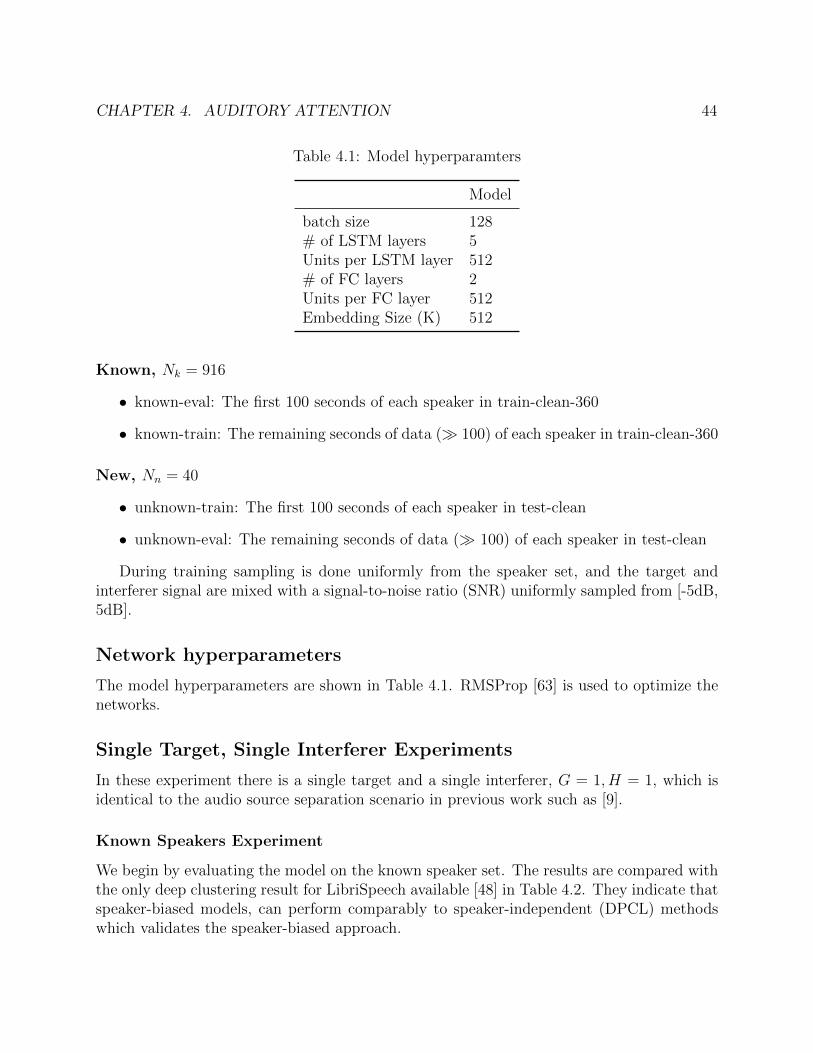
CHAPTER 4. AUDITORY ATTENTION 44
Table 4.1: Model hyperparamters
Model
batch size 128# of LSTM layers 5Units per LSTM layer 512# of FC layers 2Units per FC layer 512Embedding Size (K) 512
Known, Nk = 916
• known-eval: The first 100 seconds of each speaker in train-clean-360
• known-train: The remaining seconds of data (� 100) of each speaker in train-clean-360
New, Nn = 40
• unknown-train: The first 100 seconds of each speaker in test-clean
• unknown-eval: The remaining seconds of data (� 100) of each speaker in test-clean
During training sampling is done uniformly from the speaker set, and the target andinterferer signal are mixed with a signal-to-noise ratio (SNR) uniformly sampled from [-5dB,5dB].
Network hyperparameters
The model hyperparameters are shown in Table 4.1. RMSProp [63] is used to optimize thenetworks.
Single Target, Single Interferer Experiments
In these experiment there is a single target and a single interferer, G = 1, H = 1, which isidentical to the audio source separation scenario in previous work such as [9].
Known Speakers Experiment
We begin by evaluating the model on the known speaker set. The results are compared withthe only deep clustering result for LibriSpeech available [48] in Table 4.2. They indicate thatspeaker-biased models, can perform comparably to speaker-independent (DPCL) methodswhich validates the speaker-biased approach.
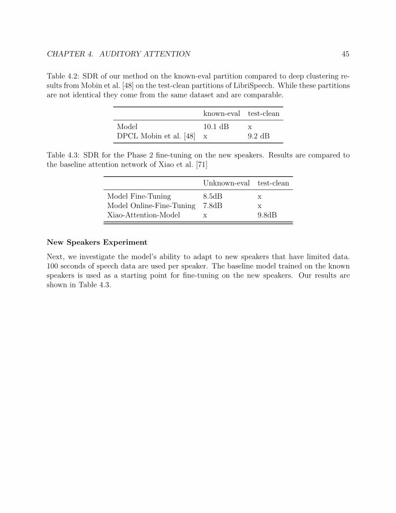
CHAPTER 4. AUDITORY ATTENTION 45
Table 4.2: SDR of our method on the known-eval partition compared to deep clustering re-sults from Mobin et al. [48] on the test-clean partitions of LibriSpeech. While these partitionsare not identical they come from the same dataset and are comparable.
known-eval test-clean
Model 10.1 dB xDPCL Mobin et al. [48] x 9.2 dB
Table 4.3: SDR for the Phase 2 fine-tuning on the new speakers. Results are compared tothe baseline attention network of Xiao et al. [71]
Unknown-eval test-clean
Model Fine-Tuning 8.5dB xModel Online-Fine-Tuning 7.8dB xXiao-Attention-Model x 9.8dB
New Speakers Experiment
Next, we investigate the model’s ability to adapt to new speakers that have limited data.100 seconds of speech data are used per speaker. The baseline model trained on the knownspeakers is used as a starting point for fine-tuning on the new speakers. Our results areshown in Table 4.3.
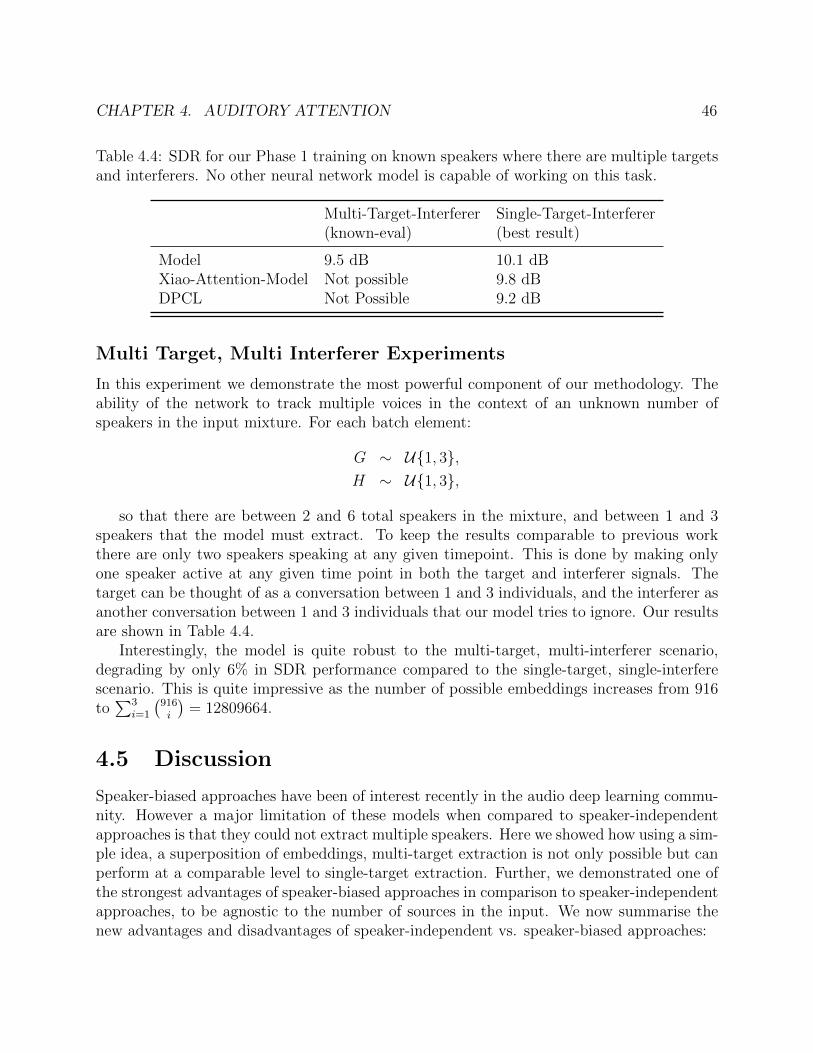
CHAPTER 4. AUDITORY ATTENTION 46
Table 4.4: SDR for our Phase 1 training on known speakers where there are multiple targetsand interferers. No other neural network model is capable of working on this task.
Multi-Target-Interferer Single-Target-Interferer(known-eval) (best result)
Model 9.5 dB 10.1 dBXiao-Attention-Model Not possible 9.8 dBDPCL Not Possible 9.2 dB
Multi Target, Multi Interferer Experiments
In this experiment we demonstrate the most powerful component of our methodology. Theability of the network to track multiple voices in the context of an unknown number ofspeakers in the input mixture. For each batch element:
G ∼ U{1, 3},H ∼ U{1, 3},
so that there are between 2 and 6 total speakers in the mixture, and between 1 and 3speakers that the model must extract. To keep the results comparable to previous workthere are only two speakers speaking at any given timepoint. This is done by making onlyone speaker active at any given time point in both the target and interferer signals. Thetarget can be thought of as a conversation between 1 and 3 individuals, and the interferer asanother conversation between 1 and 3 individuals that our model tries to ignore. Our resultsare shown in Table 4.4.
Interestingly, the model is quite robust to the multi-target, multi-interferer scenario,degrading by only 6% in SDR performance compared to the single-target, single-interferescenario. This is quite impressive as the number of possible embeddings increases from 916to∑3
i=1
(916i
)= 12809664.
4.5 Discussion
Speaker-biased approaches have been of interest recently in the audio deep learning commu-nity. However a major limitation of these models when compared to speaker-independentapproaches is that they could not extract multiple speakers. Here we showed how using a sim-ple idea, a superposition of embeddings, multi-target extraction is not only possible but canperform at a comparable level to single-target extraction. Further, we demonstrated one ofthe strongest advantages of speaker-biased approaches in comparison to speaker-independentapproaches, to be agnostic to the number of sources in the input. We now summarise thenew advantages and disadvantages of speaker-independent vs. speaker-biased approaches:
CHAPTER 4. AUDITORY ATTENTION 47
Speaker-Independent
+ Requires no prior knowledge of speakers
+ Ability to extract an arbitrary number of sources
- Requires the number of sources in the mixture to be known
Speaker-Biased
- Requires prior knowledge of speakers
+ Ability to extract an arbitrary number of sources
+ Agnostic to the number of sources in the input
A new method for deriving speaker embeddings was also developed, termed inference-embeddings. While this method did not perform as well as the reference-audio approach, littlehyperparameter tuning was done on the models. This method is also of interest because itcould resolve the remaining disadvantage of the speaker-biased approach. The idea is thatonce a baseline model is constructed, speaker embeddings are essentially voice fingerprintsthat can be used to extract a specific voice. When the model wants to learn about a newspeaker, it can find a new embedding which is different than all others it knows about,but which also causes the network to output something that sounds like human speech. Inthis chapter a supervised signal was used to validate human speech output. But instead,a discriminator in a generative adversarial network [20] could be used to ensure the newembedding corresponded to human speech.
Humans do not have the ability to simultaneously track all sources inside a sound mixture.They utilize their attention mechanism to identify and learn about new sources on-the-fly,in the spirit of continual learning. This work is a step towards more human-like sourceseparation which has substantial room for research innovation.
48
Chapter 5
Conclusion
5.1 Closing remarks
Three key questions were asked: 1) Why did the cochlea evolve to use a time-frequency code?2) How do we build human-level robust statistical models of sound? 3) How does feedback inthe auditory system guide our attention? A theoretical model based on efficient coding andleaky-integrate-and-fire (LIF) neurons was created to explain the auditory nerve response.A more efficient neural network architecture was designed which was more robust to shifts inthe data distribution. Finally, a novel algorithm was developed to allow for high-level neuralsignaling to modulate bottom-up processing to explain auditory attention. This work formsa foundation for others to continue to make progress on these questions.
Future Work
In Chapter 2 gradients of a non-smooth forwards pass, from the LIF neurons, were replacedwith a smooth backwards pass to help optimization. This wasn’t enough to prevent themodel from converging to sub-optimal local minima. One possible explanation is that smallchanges in the forwards pass still dramatically change the output, despite the changes in thebackwards pass. It would be interesting to smooth the forwards pass as well but graduallyiterate towards the non-smooth version. This might help optimization become more stable.
In Chapter 3 different neural network architectures were explored to improve generaliza-tion to new data domains. Another approach is data augmentation. The idea is to generateadditional data that is still in the class of natural sound using existing, fixed datasets. Howcould we generate more natural sound? One observation is that the real world containsmuch more reverberation, essentially short-time scale echoes, than existing datasets. Oftenaudio datasets are recorded with headsets that eliminate reverb, or in otherwise less realisticenvironments. To generate more realistic data we could simulate reverberation using a setof all pass and feedback comb filters as in the work of Schroeder [58].
In Chapter 4 a new algorithm was developed to extract multiple voices from a mixtureusing an attentional context. One shortcoming of this algorithm is that the speakers, and
CHAPTER 5. CONCLUSION 49
audio of the speakers, had to be known before hand. However, humans have no such limita-tion, we learn the voices of new speakers all the time. It would be very interesting to havethe model have a discovery mode which allows it to learn new voices. One idea for doingthis is to encourage the algorithm to find an embedding that is dissimilar to all speakerembeddings it knows about, but also causes the network to output natural sounding speech.Specifically, gradients could be taken with respect to the embedding of a loss function withtwo components. The first would be the negative sum of the mean-squared-error betweenthe current embedding and all known embeddings. The second would be the generator lossin a Generative Adversarial Network (GAN), where the output of our current model shouldbe a sound that pleases a discriminator of a GAN. The discriminator in this GAN would betrained to discriminate between speech and not-speech. Using this framework the algorithmcould become more autonomous, learning about new voices on-the-fly, and be able to extractnew voices given the correct speaker embeddings. This innovation would start to bridge thegap between the capabilities of our attentional models and those of human attention.
5.2 Next Steps
Over the last few years I’ve thought a lot about hearing science [45], deep learning modelsof sound, and how we can combine the two to help the hearing impaired hear better. Agood place to start is with a problem. In a paper called “Why do people fitted with hearingaids not wear them?” [47] McCormack et. al. found that the most significant reason peopledidn’t wear hearing aids was because a lack of speech clarity. In other words modern hearingaids are unable to help them hear the voices of their peers so they didn’t see any pointin wearing them. With further research we find that indeed everyone with hearing aidscomplains that they cannot hear voices in noisy places like restaurants and bars. And it’s aserious problem, leading to the 30 million hearing impaired Americans to be twice as likelyto develop depression [40] and two to five times more likely to develop dementia [43] due thesocial isolation they experience.
What can be done about this? In Chapter 4 a model was developed to selectively focuson a subset of voices in the context of many voices. If we think of the restaurant as mixtureof many voices, say 100, then the goal of a hearing aid should be to amplify a select fewof those voices, say 5, that originate at our table. We then see a perfect application of ourresearch, we build hearing aids that are customized for each user, to attend to the specificvoices of their friends and family and ignore everyone else. In Chapter 4 we showed thatonly a small sample of audio data was needed per target speaker to extract their voice.Therefore each user could simply collect voice samples from their peers to accomplish this.I believe there is a big opportunity to take this research outside the lab and into a productthat improves the quality of lives of tens of millions of people around the world. And ofcourse, this idea is just the beginning, continuing research in this domain will lead to evenmore fruitful methods of helping the hearing impaired.
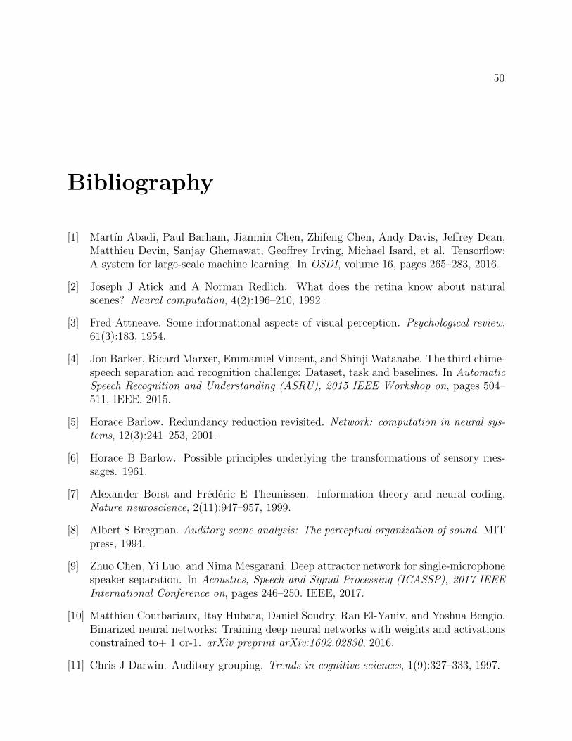
50
Bibliography
[1] Martın Abadi, Paul Barham, Jianmin Chen, Zhifeng Chen, Andy Davis, Jeffrey Dean,Matthieu Devin, Sanjay Ghemawat, Geoffrey Irving, Michael Isard, et al. Tensorflow:A system for large-scale machine learning. In OSDI, volume 16, pages 265–283, 2016.
[2] Joseph J Atick and A Norman Redlich. What does the retina know about naturalscenes? Neural computation, 4(2):196–210, 1992.
[3] Fred Attneave. Some informational aspects of visual perception. Psychological review,61(3):183, 1954.
[4] Jon Barker, Ricard Marxer, Emmanuel Vincent, and Shinji Watanabe. The third chime-speech separation and recognition challenge: Dataset, task and baselines. In AutomaticSpeech Recognition and Understanding (ASRU), 2015 IEEE Workshop on, pages 504–511. IEEE, 2015.
[5] Horace Barlow. Redundancy reduction revisited. Network: computation in neural sys-tems, 12(3):241–253, 2001.
[6] Horace B Barlow. Possible principles underlying the transformations of sensory mes-sages. 1961.
[7] Alexander Borst and Frederic E Theunissen. Information theory and neural coding.Nature neuroscience, 2(11):947–957, 1999.
[8] Albert S Bregman. Auditory scene analysis: The perceptual organization of sound. MITpress, 1994.
[9] Zhuo Chen, Yi Luo, and Nima Mesgarani. Deep attractor network for single-microphonespeaker separation. In Acoustics, Speech and Signal Processing (ICASSP), 2017 IEEEInternational Conference on, pages 246–250. IEEE, 2017.
[10] Matthieu Courbariaux, Itay Hubara, Daniel Soudry, Ran El-Yaniv, and Yoshua Bengio.Binarized neural networks: Training deep neural networks with weights and activationsconstrained to+ 1 or-1. arXiv preprint arXiv:1602.02830, 2016.
[11] Chris J Darwin. Auditory grouping. Trends in cognitive sciences, 1(9):327–333, 1997.
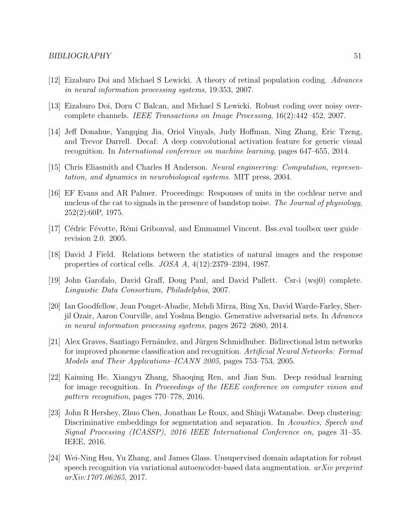
BIBLIOGRAPHY 51
[12] Eizaburo Doi and Michael S Lewicki. A theory of retinal population coding. Advancesin neural information processing systems, 19:353, 2007.
[13] Eizaburo Doi, Doru C Balcan, and Michael S Lewicki. Robust coding over noisy over-complete channels. IEEE Transactions on Image Processing, 16(2):442–452, 2007.
[14] Jeff Donahue, Yangqing Jia, Oriol Vinyals, Judy Hoffman, Ning Zhang, Eric Tzeng,and Trevor Darrell. Decaf: A deep convolutional activation feature for generic visualrecognition. In International conference on machine learning, pages 647–655, 2014.
[15] Chris Eliasmith and Charles H Anderson. Neural engineering: Computation, represen-tation, and dynamics in neurobiological systems. MIT press, 2004.
[16] EF Evans and AR Palmer. Proceedings: Responses of units in the cochlear nerve andnucleus of the cat to signals in the presence of bandstop noise. The Journal of physiology,252(2):60P, 1975.
[17] Cedric Fevotte, Remi Gribonval, and Emmanuel Vincent. Bss eval toolbox user guide–revision 2.0. 2005.
[18] David J Field. Relations between the statistics of natural images and the responseproperties of cortical cells. JOSA A, 4(12):2379–2394, 1987.
[19] John Garofalo, David Graff, Doug Paul, and David Pallett. Csr-i (wsj0) complete.Linguistic Data Consortium, Philadelphia, 2007.
[20] Ian Goodfellow, Jean Pouget-Abadie, Mehdi Mirza, Bing Xu, David Warde-Farley, Sher-jil Ozair, Aaron Courville, and Yoshua Bengio. Generative adversarial nets. In Advancesin neural information processing systems, pages 2672–2680, 2014.
[21] Alex Graves, Santiago Fernandez, and Jurgen Schmidhuber. Bidirectional lstm networksfor improved phoneme classification and recognition. Artificial Neural Networks: FormalModels and Their Applications–ICANN 2005, pages 753–753, 2005.
[22] Kaiming He, Xiangyu Zhang, Shaoqing Ren, and Jian Sun. Deep residual learningfor image recognition. In Proceedings of the IEEE conference on computer vision andpattern recognition, pages 770–778, 2016.
[23] John R Hershey, Zhuo Chen, Jonathan Le Roux, and Shinji Watanabe. Deep clustering:Discriminative embeddings for segmentation and separation. In Acoustics, Speech andSignal Processing (ICASSP), 2016 IEEE International Conference on, pages 31–35.IEEE, 2016.
[24] Wei-Ning Hsu, Yu Zhang, and James Glass. Unsupervised domain adaptation for robustspeech recognition via variational autoencoder-based data augmentation. arXiv preprintarXiv:1707.06265, 2017.
BIBLIOGRAPHY 52
[25] Ke Hu and DeLiang Wang. An unsupervised approach to cochannel speech separation.IEEE Transactions on audio, speech, and language processing, 21(1):122–131, 2013.
[26] Yusuf Isik, Jonathan Le Roux, Zhuo Chen, Shinji Watanabe, and John R Her-shey. Single-channel multi-speaker separation using deep clustering. arXiv preprintarXiv:1607.02173, 2016.
[27] Lukasz Kaiser and Ilya Sutskever. Neural gpus learn algorithms. arXiv preprintarXiv:1511.08228, 2015.
[28] Yan Karklin and Eero P Simoncelli. Efficient coding of natural images with a populationof noisy linear-nonlinear neurons. In NIPS, volume 24, pages 999–1007, 2011.
[29] Emine Merve Kaya and Mounya Elhilali. Modelling auditory attention. PhilosophicalTransactions of the Royal Society B: Biological Sciences, 372(1714):20160101, 2017.
[30] Diederik P Kingma and Max Welling. Auto-encoding variational bayes. arXiv preprintarXiv:1312.6114, 2013.
[31] Keisuke Kinoshita, Marc Delcroix, Takuya Yoshioka, Tomohiro Nakatani, Armin Sehr,Walter Kellermann, and Roland Maas. The reverb challenge: A common evaluationframework for dereverberation and recognition of reverberant speech. In Applicationsof Signal Processing to Audio and Acoustics (WASPAA), 2013 IEEE Workshop on,pages 1–4. IEEE, 2013.
[32] Alex Krizhevsky, Ilya Sutskever, and Geoffrey E Hinton. Imagenet classification withdeep convolutional neural networks. In Advances in neural information processing sys-tems, pages 1097–1105, 2012.
[33] Michael F Land and Dan-Eric Nilsson. Animal eyes. Oxford University Press, 2012.
[34] Quoc V Le, Alexandre Karpenko, Jiquan Ngiam, and Andrew Y Ng. Ica with reconstruc-tion cost for efficient overcomplete feature learning. In Advances in Neural InformationProcessing Systems, pages 1017–1025, 2011.
[35] Jonathan Le Roux, JR Hershey, A Liutkus, F Stoter, ST Wisdom, and H Erdogan.Sdr–half-baked or well done? Mitsubishi Electric Research Laboratories (MERL), Cam-bridge, MA, USA, Tech. Rep, 2018.
[36] Yann LeCun, Leon Bottou, Yoshua Bengio, and Patrick Haffner. Gradient-based learn-ing applied to document recognition. Proceedings of the IEEE, 86(11):2278–2324, 1998.
[37] Yann LeCun, Yoshua Bengio, and Geoffrey Hinton. Deep learning. nature, 521(7553):436, 2015.
[38] Jun Haeng Lee, Tobi Delbruck, and Michael Pfeiffer. Training deep spiking neuralnetworks using backpropagation. Frontiers in Neuroscience, 10, 2016.
BIBLIOGRAPHY 53
[39] Michael S Lewicki. Efficient coding of natural sounds. Nature neuroscience, 5(4):356–363, 2002.
[40] Chuan-Ming Li, Xinzhi Zhang, Howard J Hoffman, Mary Frances Cotch, Christa L The-mann, and M Roy Wilson. Hearing impairment associated with depression in us adults,national health and nutrition examination survey 2005-2010. JAMA otolaryngology–head & neck surgery, 140(4):293–302, 2014.
[41] Jinyu Li, Li Deng, Yifan Gong, and Reinhold Haeb-Umbach. An overview of noise-robust automatic speech recognition. IEEE/ACM Transactions on Audio, Speech, andLanguage Processing, 22(4):745–777, 2014.
[42] MC Liberman. Single-neuron labeling in the cat auditory nerve. Science, 216(4551):1239–1241, 1982.
[43] Frank R Lin, E Jeffrey Metter, Richard J OBrien, Susan M Resnick, Alan B Zonderman,and Luigi Ferrucci. Hearing loss and incident dementia. Archives of neurology, 68(2):214–220, 2011.
[44] Yi Luo and Nima Mesgarani. Tasnet: time-domain audio separation network for real-time, single-channel speech separation. In 2018 IEEE International Conference onAcoustics, Speech and Signal Processing (ICASSP), pages 696–700. IEEE, 2018.
[45] Richard F Lyon. Human and machine hearing. Cambridge University Press, 2017.
[46] Stephane G Mallat and Zhifeng Zhang. Matching pursuits with time-frequency dictio-naries. IEEE Transactions on signal processing, 41(12):3397–3415, 1993.
[47] Abby McCormack and Heather Fortnum. Why do people fitted with hearing aids notwear them? International journal of audiology, 52(5):360–368, 2013.
[48] Shariq Mobin, Brian Cheung, and Bruno Olshausen. Generalization challenges for neuralarchitectures in audio source separation. arXiv preprint arXiv:1803.08629, 2018.
[49] Peter O’Connor and Max Welling. Deep spiking networks. arXiv preprintarXiv:1602.08323, 2016.
[50] Bruno A Olshausen and David J Field. Emergence of simple-cell receptive field proper-ties by learning a sparse code for natural images. Nature, 381(6583):607, 1996.
[51] Bruno A Olshausen and Kevin N O’Connor. A new window on sound. nature neuro-science, 5(4):292, 2002.
[52] AR Palmer and IJ Russell. Phase-locking in the cochlear nerve of the guinea-pig andits relation to the receptor potential of inner hair-cells. Hearing research, 24(1):1–15,1986.
BIBLIOGRAPHY 54
[53] Vassil Panayotov, Guoguo Chen, Daniel Povey, and Sanjeev Khudanpur. Librispeech:an asr corpus based on public domain audio books. In Acoustics, Speech and SignalProcessing (ICASSP), 2015 IEEE International Conference on, pages 5206–5210. IEEE,2015.
[54] Colin Raffel, Brian McFee, Eric J Humphrey, Justin Salamon, Oriol Nieto, DawenLiang, Daniel PW Ellis, and C Colin Raffel. mir eval: A transparent implementationof common mir metrics. In In Proceedings of the 15th International Society for MusicInformation Retrieval Conference, ISMIR. Citeseer, 2014.
[55] Alberto Recio-Spinoso, Andrei N Temchin, Pim van Dijk, Yun-Hui Fan, and Mario ARuggero. Wiener-kernel analysis of responses to noise of chinchilla auditory-nerve fibers.Journal of neurophysiology, 93(6):3615–3634, 2005.
[56] Jerzy E Rose, John F Brugge, David J Anderson, and Joseph E Hind. Phase-lockedresponse to low-frequency tones in single auditory nerve fibers of the squirrel monkey.Journal of neurophysiology, 30(4):769–793, 1967.
[57] Jan Schnupp, Israel Nelken, and Andrew King. Auditory neuroscience: Making senseof sound. MIT press, 2011.
[58] Manfred R Schroeder. Natural sounding artificial reverberation. Journal of the AudioEngineering Society, 10(3):219–223, 1962.
[59] William Arthur Sethares. Rhythm and transforms. Springer Science & Business Media,2007.
[60] Siddharth Sigtia, Emmanouil Benetos, and Simon Dixon. An end-to-end neural networkfor polyphonic piano music transcription. IEEE/ACM Transactions on Audio, Speechand Language Processing (TASLP), 24(5):927–939, 2016.
[61] Evan C Smith and Michael S Lewicki. Efficient auditory coding. Nature, 439(7079):978–982, 2006.
[62] Gonzalo Terreros and Paul H Delano. Corticofugal modulation of peripheral auditoryresponses. Frontiers in systems neuroscience, 9:134, 2015.
[63] Tijmen Tieleman and Geoffrey Hinton. Lecture 6.5-rmsprop: Divide the gradient by arunning average of its recent magnitude. COURSERA: Neural networks for machinelearning, 4(2):26–31, 2012.
[64] Antonio Torralba and Alexei A Efros. Unbiased look at dataset bias. In ComputerVision and Pattern Recognition (CVPR), 2011 IEEE Conference on, pages 1521–1528.IEEE, 2011.

BIBLIOGRAPHY 55
[65] Eric Tzeng, Judy Hoffman, Kate Saenko, and Trevor Darrell. Adversarial discriminativedomain adaptation. In Computer Vision and Pattern Recognition (CVPR), volume 1,page 4, 2017.
[66] Mats Ulfendahl and Ake Flock. Outer hair cells provide active tuning in the organ ofcorti. Physiology, 13(3):107–111, 1998.
[67] Emmanuel Vincent, Remi Gribonval, and Cedric Fevotte. Performance measurementin blind audio source separation. IEEE transactions on audio, speech, and languageprocessing, 14(4):1462–1469, 2006.
[68] Quan Wang, Hannah Muckenhirn, Kevin Wilson, Prashant Sridhar, Zelin Wu, JohnHershey, Rif A Saurous, Ron J Weiss, Ye Jia, and Ignacio Lopez Moreno. Voicefilter:Targeted voice separation by speaker-conditioned spectrogram masking. arXiv preprintarXiv:1810.04826, 2018.
[69] Bo Wen, Grace I Wang, Isabel Dean, and Bertrand Delgutte. Dynamic range adaptationto sound level statistics in the auditory nerve. Journal of Neuroscience, 29(44):13797–13808, 2009.
[70] Kevin Wilson, Michael Chinen, Jeremy Thorpe, Brian Patton, John Hershey, Rif ASaurous, Jan Skoglund, and Richard F Lyon. Exploring tradeoffs in models for low-latency speech enhancement. In 2018 16th International Workshop on Acoustic SignalEnhancement (IWAENC), pages 366–370. IEEE, 2018.
[71] Xiong Xiao, Zhuo Chen, Takuya Yoshioka, Hakan Erdogan, Changliang Liu, DimitriosDimitriadis, Jasha Droppo, and Yifan Gong. Single-channel speech extraction usingspeaker inventory and attention network. In ICASSP 2019-2019 IEEE InternationalConference on Acoustics, Speech and Signal Processing (ICASSP), pages 86–90. IEEE,2019.
[72] Dong Yu, Morten Kolbæk, Zheng-Hua Tan, and Jesper Jensen. Permutation invarianttraining of deep models for speaker-independent multi-talker speech separation. In 2017IEEE International Conference on Acoustics, Speech and Signal Processing (ICASSP),pages 241–245. IEEE, 2017.
[73] Fisher Yu and Vladlen Koltun. Multi-scale context aggregation by dilated convolutions.arXiv preprint arXiv:1511.07122, 2015.
[74] Katerina Zmolikova, Marc Delcroix, Keisuke Kinoshita, Takuya Higuchi, AtsunoriOgawa, and Tomohiro Nakatani. Speaker-aware neural network based beamformer forspeaker extraction in speech mixtures. In Interspeech, pages 2655–2659, 2017.