Inflation Bets or Deflation Hedges?

The Changing Risks of Nominal Bonds

John Y. Campbell, Adi Sunderam, and Luis M. Viceira

Harvard University

August 2007

This research was supported by the U.S. Social Security Administration through

grant #10-P-98363-1-04 to the National Bureau of Economic Research as part of the

SSA Retirement Research Consortium. The findings and conclusions expressed are

solely those of the authors and do not represent the views of SSA, any agency of the

Federal Government, or the NBER. We also acknowledge the support of the National

Science Foundation under grant no. 0214061 to Campbell, and of Harvard Business

School Research Funding to Viceira.

Abstract

The covariance between US Treasury bond returns and stock returns has moved

considerably over time. While it was slightly positive on average in the period 1953—

2005, it was particularly high in the early 1980’s and negative in the early 2000’s. This

paper specifies and estimates a model in which the nominal term structure of interest

rates is driven by four state variables: the real interest rate, risk aversion, expected

inflation, and the covariance between nominal variables and the real economy. Log

nominal bond yields and term premia are quadratic in these state variables, with

term premia determined mainly by the product of risk aversion and the nominal-real

covariance. The concavity of the yield curve–the level of intermediate-term bond

yields, relative to the average of short- and long-term bond yields–is a good proxy

for the level of term premia.

1 Introduction

Are nominal bonds risky investments, which investors must be rewarded to hold?

Or are they safe investments, whose price movements are either inconsequential or

possibly even beneficial to investors as a hedge against other risks?

This question can be answered in a number of ways. A first approach is to measure

the covariance of nominal bond returns with some measure of investor well-being.

According to the Capital Asset Pricing Model (CAPM), for example, investor well-

being can be summarized by the level of aggregate wealth. It follows that the risk of

bonds can be measured by the covariance of bond returns with returns on the market

portfolio, often proxied by a broad stock index. According to the Consumption

CAPM, investor well-being can be summarized by the level of aggregate consumption

and so the risk of bonds can be measured by the covariance of bond returns with

aggregate consumption growth.

A second approach is to measure the risk premium on nominal bonds, either from

average realized excess returns on bonds or from the average yield spread on long-

term bonds over short-term bills. If this risk premium is large, then presumably

investors regard bonds as risky.

These approaches are appealing because they are straightforward and direct. Un-

fortunately, the answers they give appear to depend sensitively on the particular sam-

ple period that is used. The covariance of nominal bond returns with stock returns,

for example, is extremely unstable over time and even switches sign (Guidolin and

Timmermann 2004, Baele, Bekaert, and Inghelbrecht 2007, Viceira 2007). In some

periods, notably the late 1970’s and early 1980’s, bond and stock returns move closely

together, implying that bonds have a high CAPM beta and are relatively risky. In

other periods, notably the late 1990’s and early 2000’s, bond and stock returns are

negatively correlated, implying that bonds have a negative beta and can be used to

hedge shocks to aggregate wealth. The average level of the yield spread is also un-

stable over time as pointed out by Fama (2006) among others. An intriguing fact is

that the movements in the average yield spread seem to line up to some degree with

the movements in the CAPM beta of bonds. The average yield spread was high in

the early 1980’s and much lower in the late 1990’s.

A third approach to measuring the risks of bonds is to decompose bond returns

into several components arising from different underlying shocks. Nominal bond

1

returns are driven by movements in real interest rates, inflation expectations, and

the risk premium on nominal bonds over short-term bills. The variances of these

components, and their correlations with investor well-being, determine the overall

risk of nominal bonds. Campbell and Ammer (1993), for example, estimate that

over the period 1952—1987, real interest rate shocks moved stocks and bonds in the

same direction but had relatively low volatility; shocks to long-term expected inflation

moved stocks and bonds in opposite directions; and shocks to risk premia again moved

stocks and bonds in the same direction. The overall effect of these opposing forces was

a relatively low correlation between stock and bond returns. However Campbell and

Ammer assume that the underlying shocks have constant variances and correlations

throughout their sample period, and so their approach fails to explain changes in

covariances over time.2

Economic theory provides some guidance in modelling the risks of underlying

shocks to bond returns. For example, consumption shocks raise real interest rates

if consumption growth is positively autocorrelated (Campbell 1986, Gollier 2005); in

this case real bonds hedge consumption risk and should have negative risk premia. If

the level of consumption is stationary around a trend, however, consumption growth is

negatively autocorrelated, real bonds are exposed to consumption risk, and real bond

premia should be positive. Inflation shocks are positively correlated with economic

growth if demand shocks move the macroeconomy up and down a stable Phillips

Curve; but inflation is negatively correlated with economic growth if supply shocks

move the Phillips Curve in and out. Shocks to risk premia move stocks and bonds in

the same direction if bonds are risky, and in opposite directions if bonds are hedges

against risk (Connolly, Stivers, and Sun 2005). These shocks may be correlated with

shocks to consumption if investors’ risk aversion moves with the state of the economy,

as in models with habit formation (Campbell and Cochrane 1999).

In this paper we specify and estimate a term structure model that is designed to

allow the correlations of shocks, in particular the correlation of inflation with real

variables, to change over time. By specifying stochastic processes for real interest

rates, expected inflation, and investor risk aversion, we can solve for the complete

term structure at each point in time and understand the way in which bond market

risks have evolved.

Our approach extends a number of recent term structure models. Bekaert, En-

gstrom, and Grenadier (BEG, 2004), Wachter (2006), and Buraschi and Jiltsov (2007)

2See also Barsky (1989) and Shiller and Beltratti (1992).

2

all specify term structure models in which risk aversion varies over time, influencing

the shape of the yield curve. These papers take care to remain in the affine class

(Dai and Singleton 2002). BEG and other recent authors including Mamaysky (2002)

and d’Addona and Kind (2005) extend affine term structure models to price stocks

as well as bonds. Our introduction of a time-varying correlation between inflation

and real shocks takes us outside the affine class; our model, like those of Constan-

tinides (1992) and Ahn, Dittmar and Gallant (2002), is linear-quadratic. To solve

it, we use a general result on the expected value of the exponential of a non-central

chi-squared distribution which we take from the Appendix to Campbell, Chan, and

Viceira (2003). We estimate our model using a Kalman filter approach, an extension

of the method used in Campbell and Viceira (2001, 2002).

The organization of the paper is as follows. Section 2 presents our model of the

nominal term structure. Section 3 describes our estimation method and presents

parameter estimates and historical fitted values for the unobservable state variables

of the model. Section 4 discusses the implications of the model for the shape of the

yield curve and the movements of risk premia on nominal bonds. Section 5 concludes.

2 A Quadratic Bond Pricing Model

We start by formulating a model which, in the spirit of Campbell and Viceira (2001,

2002), accounts for the term structure of both real interest rates and nominal interest

rates. However, unlike their model, this model allows for time variation in the risk

premia on both real and nominal assets, and for time variation in the correlation

between the real economy and inflation and thus between the excess returns on real

assets and the returns on nominal assets. The model for the real term structure of

interest rates allows for time variation in both real interest rates and risk premia,

yet it is simple enough that real bond prices have an exponential affine structure.

The nominal side of the model allows for time variation in expected inflation, the

volatility of inflation, and the conditional correlation of inflation with the real side

of the economy. This results in a nominal term structure where bond yields are

linear-quadratic functions of the vector of state variables.

3

2.1 An affine model of the real term structure

We pose a model for the term structure of real interest rates that has a simple linear

structure. We assume that the log of the real stochastic discount factor (SDF)mt+1 =log (Mt+1) follows a linear-quadratic, conditionally heteroskedastic process:

−mt+1 = xt +σ2m2z2t + ztεm,t+1, (1)

where both xt and zt follow standard AR(1) processes,

xt+1 = μx (1− φx) + φxxt + εx,t+1, (2)

zt+1 = μz (1− φz) + φzzt + εz,t+1, (3)

and εm,t+1, εx,t+1, and εx,t+1 are jointly normally distributed zero-mean shocks withconstant variance-covariance matrix. We allow these shocks to be cross-correlated,

and adopt the notation σ2i to describe the variance of shock εi, and σij to describethe covariance between shock εi and shock εj. In this model, σm always appears

premultiplied by zt in all pricing equations. This implies that we are unable to

identify σm separately from zt. Thus without loss of generality we set σm to an

arbitrary value of 1.

Even though shocks ε are homoskedastic, the log real SDF itself is conditionallyheteroskedastic, with

Vart (mt+1) = z2t .

Thus the state variable zt determines time-variation in the volatility of the SDF or,equivalently, in the price of aggregate market risk. In fact, we can interpret our

model for the real SDF as a reduced form of a structural model in which aggregate

risk aversion changes over time as a function of zt, as in the habit consumption modelof Campbell and Cochrane (1999). While our model does not constrain zt to remainalways positive, our empirical estimates do have this property.

The second state variable xt determines the dynamics of the short-term log real

interest rate. The price of a single-period zero-coupon real bond satisfies

P1,t = Et [exp {mt+1}] ,so that its yield y1t = − log(P1,t) equals

y1t = −Et [mt+1]− 12Vart (mt+1) = xt. (4)

4

Thus the model (1)-(3) allows for time variation in risk premia, yet it preserves simple

linear dynamics for the short-term real interest rate.

This model implies that the real term structure of interest rates is affine in the

state variables xt and zt. Standard calculations (Campbell, Lo, and MacKinlay 1997,Chapter 11) show that the price of a zero-coupon real bond with n periods to maturityis given by

Pn,t = exp {An +Bx,nxt +Bz,nzt} ,where

An = An−1 +Bx,n−1μx (1− φx) +Bz,n−1μz (1− φz)

+1

2B2x,n−1σ

2x +

1

2B2z,n−1σ

2z +Bx,n−1Bz,n−1σxz,

Bx,n = −1 +Bx,n−1φx,

and

Bz,n = Bz,n−1φz −Bx,n−1σmx −Bz,n−1σmz,

with A1 = 0, Bx,1 = −1, and Bz,1 = 0. Note that Bx,n < 0 for all n when φx > 0.Details of these calculations are presented in the Appendix to this paper (Campbell,

Sunderam, and Viceira 2007).

The excess log return on a n-period zero-coupon real bond over a 1-period realbond is given by

rn,t+1 − r1,t+1 = pn−1,t+1 − pn,t + p1,t

= −µ1

2B2x,n−1σ

2x +

1

2B2z,n−1σ

2z +Bx,n−1Bz,n−1σxz

¶+(Bx,n−1σmx +Bz,n−1σmz) zt

+Bx,n−1εx,t+1 +Bz,n−1εz,t+1, (5)

where the first term is a Jensen’s inequality correction, the second term describes the

log of the expected excess return on real bonds, and the third term describes shocks

to realized excess returns. Note that r1,t+1 ≡ y1,t.

It follows from (5) that the conditional risk premium on real bonds is

Et [rn,t+1 − r1,t+1] +1

2Vart (rn,t+1 − r1,t+1) = (Bx,n−1σmx +Bz,n−1σmz) zt, (6)

5

which is proportional to the state variable zt. The coefficient of proportionality is(Bx,n−1σmx + Bz,n−1σmz), which can take either sign. It is zero, and thus real bondrisk premia are zero, when σmx = 0, that is, when shocks to real interest rates areuncorrelated with the stochastic discount factor.3 Real bond risk premia are also

zero when the state variable zt is zero, for then the stochastic discount factor is aconstant which implies risk-neutral asset pricing.

To gain intuition about the behavior of risk premia on real bonds, consider the

simple case where σmz = 0 and σmx > 0. Since Bx,n−1 < 0, this implies that realbond risk premia are negative. The reason for this is that with positive σmx, the real

interest rate tends to rise in good times and fall in bad times. Since real bond returns

move opposite the real interest rate, real bonds are countercyclical assets that hedge

against economic downturns and command a negative risk premium. Empirically,

however, we estimate a negative σmx; this implies procyclical real bond returns that

command a positive risk premium, increasing with the level of risk aversion.

2.2 Pricing equities

We want our model to fit the changing covariance of bonds and stocks, and so we

must specify a process for the equity return within the model. Following Campbell

and Viceira (2001), we model shocks to realized stock returns as a linear combination

of shocks to the real rate and shocks to the log stochastic discount factor:

re,t+1 − Et re,t+1 = βexεx,t+1 + βemεm,t+1 + εe,t+1, (7)

where εe,t+1 is an identically and independently distributed shock uncorrelated with allother shocks in the model. This shock captures variation in equity returns unrelated

to real interest rates, and unpriced because uncorrelated with the SDF.

Substituting (7) into the no-arbitrage condition Et [Mt+1Rt+1] = 1, the conditionalequity risk premium is given by

Et [re,t+1 − r1,t+1] +1

2Vart (re,t+1 − r1,t+1) =

¡βexσxm + βemσ

2m

¢zt. (8)

The equity premium, like all risk premia in our model, is proportional to risk aversion

zt. It depends not only on the direct sensitivity of stock returns to the SDF, but also

3Note that σmx = 0 implies not only Bx,n = 0, but also Bz,n = 0, for all n.

6

on the sensitivity of stock returns to the real interest rate and the covariance of the

real interest rate with the SDF.

2.3 A model of time-varying inflation risk

To price nominal bonds, we need to specify a model for inflation or, more precisely, for

the reciprocal of inflation, which determines the real value of the nominal payments

made by the bonds. We assume that log inflation πt = log (Πt) follows a linearconditionally heteroskedastic process:

πt+1 = ξt +σ2ψ2ψ2t + ψtεπ,t+1, (9)

where expected log inflation ξt and ψt follow

ξt+1 = μξ¡1− φξ

¢+ φξξt + ψtεξ,t+1, (10)

ψt+1 = μψ¡1− φψ

¢+ φψψt + εψ,t+1, (11)

and επ,t+1, εξ,t+1, and εψ,t+1 are again jointly normally distributed zero-mean shockswith a constant variance-covariance matrix. We allow these shocks to be cross-

correlated with the shocks to mt+1, xt+1, and zt+1, and use the same notation asin section 2.1 to denote their variances and covariances.

A large empirical literature in macroeconomics has documented changing volatility

in inflation. In fact, the popular ARCH model of conditional heteroskedasticity

(Engle 1982) was first applied to inflation. Our model captures this heteroskedasticity

using a persistent state variable ψt. We assume that this variable drives the volatility

of expected inflation as well as the volatility of realized inflation. Since we model

ψt as an AR(1) process, it can change sign. The sign of ψt does not affect the

variances of expected or realized inflation or the covariance between them, because

these moments depend on the square ψ2t . However the sign of ψt does determine the

sign of the covariance between expected and realized inflation, on the one hand, and

the real economy, on the other hand.

The process for realized inflation, equation (9), is formally similar to the process

for the log SDF (1), in the sense that it includes a Jensen’s inequality correction

term. The inclusion of this term simplifies the process for the reciprocal of inflation

7

by making the log of the conditional mean of 1/Πt+1 the negative of expected log

inflation ξt. This in turn simplifies the pricing of short-term nominal bonds.

The real cash flow on a 1-period nominal bond is simply 1/Πt+1. Thus the price

of the bond is given by

P $1,t = Et [exp {mt+1 − πt+1}] , (12)

so the log short-term nominal rate y$1,t+1 = − log¡P $1,t¢is

y$1,t+1 = −Et [mt+1 − πt+1]− 12Vart (mt+1 − πt+1)

= xt + ξt − σmπztψt, (13)

where we have used the fact that exp {mt+1 − πt+1} is conditionally lognormally dis-tributed given our assumptions.

Equation (13) shows that the log of the nominal short rate is the sum of the log

real interest rate, expected log inflation, and a nonlinear term that accounts for the

correlation between shocks to inflation and shocks to the stochastic discount factor.

If inflation is uncorrelated with the SDF (σmπ = 0), the nonlinear term is zero and

the Fisher equation holds: that is, the nominal short rate is simply the real short rate

plus expected inflation.

It is straightforward to show that the nonlinear term in (13) is the expected

excess return on a single-period nominal bond over a single-period real bond. Thus

it measures the inflation risk premium at the short end of the term structure. It

equals the conditional covariance between realized inflation and the log of the SDF:

Covt (mt+1, πt+1) = −σmπztψt. (14)

When this covariance is positive, short-term nominal bonds are risky assets that have

a positive risk premium because they tend to have unexpectedly low real payoffs

in bad times. Of course, this premium increases with risk aversion zt. When thecovariance is negative, short-term nominal bonds hedge real risk; they command a

negative risk premium which becomes even more negative as aggregate risk aversion

increases.

The covariance between inflation and the SDF is determined by the product of

two state variables, zt and ψt. Although both variables influence the magnitude of

8

the covariance, its sign is determined in practice only by ψt because, even though we

do not constrain zt to be positive, we estimate it to be so in our sample, consistentwith the notion that zt is a proxy for aggregate risk aversion. Therefore, the statevariable ψt controls not only the conditional volatility of inflation, but also the sign

of the correlation between inflation and the SDF.

This property of the single-period nominal risk premium carries over to the entire

nominal term structure. In our model the risk premium on real assets varies over

time and increases or decreases as a function of aggregate risk aversion, as shown in

(6) or (8). The risk premium on nominal bonds varies over time as a function of

both aggregate risk aversion and the covariance between inflation and the real side of

the economy. If this covariance switches sign, so will the risk premium on nominal

bonds. At times when inflation is procyclical–as will be the case if the macroecon-

omy moves along a stable Phillips Curve–nominal bond returns are countercyclical,

making nominal bonds desirable hedges against business cycle risk. At times when

inflation is countercyclical–as will be the case if the economy is affected by supply

shocks or changing inflation expectations that shift the Phillips Curve in or out–

nominal bond returns are procyclical and investors demand a positive risk premium

to hold them.

The conditional covariance between the SDF and inflation also determines the

covariance between the excess returns on real and nominal assets. Consider for

example the conditional covariance between the return on a one-period nominal bond

and the return on equities. From (7) and (9), this covariance is given by

Covt¡re,t+1 − r1,t+1, y

$1,t+1 − πt+1 − r1,t+1

¢= − (βexσxπ + βemσmπ)ψt,

which moves over time and can change sign. This implies that we can identify the

dynamics of the state variable ψt from the dynamics of the conditional covariance of

between equities and nominal bonds.

2.4 The nominal term structure

Equation (13) shows that the log nominal short rate is a linear-quadratic function of

the state variables in our model. We show in the Appendix that this property carries

over to the entire zero-coupon nominal term structure. The price of a n-period zero-coupon nominal bond is an exponential linear-quadratic function of the vector of state

9

variables:

P $n,t = exp

©A$n +B$

x,nxt +B$z,nzt +B$

ξ,nξt +B$ψ,nψt + C$

z,nz2t + C$

ψ,nψ2t + C$

zψ,nztψt

ª,

(15)

where the coefficients A$n, B$i,n, and C$

i,n solve a set of recursive equations given in

the Appendix. These coefficients are functions of the maturity of the bond (n) andthe coefficients that determine the stochastic processes for real and nominal variables.

From equation (13), it is immediate to see that B$x,1 = B$

ξ,1 = −1, C$zψ,1 = σmπ, and

that the remaining coefficients are zero at n = 1.

We can now characterize the log return on long-term nominal zero-coupon bonds in

excess of the short-term nominal interest rate. Since bond prices are not exponential

linear functions of the state variables, their returns are not conditionally lognormally

distributed. But we can still find an analytical expression for their conditional ex-

pected returns. We show in the Appendix that the log of the conditional expected

gross excess return on an n-period zero-coupon nominal bond is given by

log Et

"P $n−1,t+1P $n,t

#− Et

£r$1,t+1

¤= λz,nzt + λψ,nψt + βz,nz

2t + βψ,nψ

2t + βzψ,nztψt, (16)

where r$1,t+1 ≡ y$1,t is known at time t, and the coefficients λi,n and βi,n are functions

of the coefficients A$n, B$i,n, and C

$i,n and thus are functions of bond maturity and the

underlying stochastic processes for real and nominal variables. Explicit expressions

for λi,n and βi,n are given in Appendix X.

Equation (15) shows that our model implies a nominal term structure of interest

rates which is a linear-quadratic function of the vector of state variables. Log bond

prices are affine functions of the short-term real interest rate (xt) and expected in-flation (ξt), and quadratic functions of risk aversion (zt) and inflation volatility (ψt).

Thus our model naturally generates four factors that explain bond yields. Equa-

tion (16) shows that expected log bond excess returns are time varying. They vary

quadratically with risk aversion and inflation volatility, and linearly with the covari-

ance between the log real SDF and inflation (ztψt). In this model, bond risk premia

can be either positive or negative as ψt switches sign over time.

10

2.5 Special cases

Our general quadratic term structure model nests three important constrained mod-

els. First, if we constrain zt and ψt to be constant, our model reduces to the two-factor

affine yield model of Campbell and Viceira (2001, 2002), where both real bond risk

premia and nominal bond risk premia are constant, and the factors are the short-term

real interest rate (xt) and expected inflation (ξt). Second, if we constrain only ψt to

be constant over time, our model becomes a three-factor affine yield model where

both real bond risk premia and nominal bond risk premia vary in proportion to ag-

gregate risk aversion (zt). This model captures the spirit of recent work on the termstructure of interest rates by Bekaert, Engstrom, and Grenadier (2004), Buraschi and

Jiltsov (2006), Wachter (2006) and others in which time-varying risk aversion is the

only cause of time variation in bond risk premia. Finally, if we constrain only ztto be constant over time, our model reduces to a single-factor affine yield model for

the term structure of real interest rates, and a linear-quadratic model for the term

structure of nominal interest rates. In this constrained model, real bond risk premia

are constant, but nominal bond risk premia vary with inflation volatility.

Since the coefficients of the nominal bond pricing function are complicated func-

tions of the parameters of the model, we now present estimates of these parameters,

and discuss the properties of bond prices and bond returns given our estimates.

3 Model Estimation

3.1 Data and estimation methodology

The term structure model presented in Section 2 generates nominal bond yields which

are linear-quadratic functions of a vector of latent state variables. We now take this

model to the data, and present estimates of the model based on a standard Kalman

filter approach. Given the nonlinear structure of the model, this inherently linear

approach does not produce maximum likelihood estimates of the parameters of the

model, but rather quasi-maximum likelihood estimates. Although these estimates are

not efficient, they are still consistent and asymptotically normal. They also provide

us with a reasonable check of the ability of our data to explain important aspects

of the time series and cross-sectional behavior of interest rates. Moreover, these

11

estimates provide useful initial values for the Efficient Method of Moments of Gallant

and Tauchen (1996), which we plan to implement in the future to obtain efficient

estimates of the parameters of the model.

The Kalman filter approach starts with the specification of a system of measure-

ment equations that relate observable variables to the vector of state variables. The

filter uses these equations to infer the behavior of the latent state variables of the

model.

Our first set of measurement equations relates observable nominal bond yields to

the vector of state variables. Specifically, we use the relation between nominal zero-

coupon bond log yields y$n,t = − log(P $n,t)/n and the vector of state variables implied

by equation (15). We use monthly yields on constant maturity 3-month, 1-year, 3-

year and 10-year zero-coupon nominal bonds for the period January 1953-December

2005. This dataset is spliced together from two sources. From January 1953 through

July 1971 we use data from McCulloch and Kwon (1993) and from August 1971

through December 2005, we use data from the Federal Reserve Board constructed by

Gürkaynak, Sack, and Wright (2006). We assume that bond yields are measured with

errors, which are uncorrelated with each other and with the structural shocks of the

model.

To this set of equations we add a second set of four measurement equations. The

first equation in this set is given by equation (9), which relates observed inflation

rates to expected inflation and inflation volatility, plus a measurement error term.

The second is the equation for realized log equity returns re,t+1 implied by (4), (7),and (8).

The third additional measurement equation uses the dividend yield on equities

De,t/Pe,t to identify zt as

De,t

Pe,t= d0 + d1zt + εD/P,t+1, (17)

where εD/P,t+1 is a measurement error term uncorrelated with the fundamental shocks

of the model. This measurement equation is motivated by the fact that the dividend

yield is known to forecast future equity returns, and that in our model expected equity

excess returns are proportional to zt, as shown in (8). Thus we are effectively proxyingaggregate risk aversion with a linear transformation of the aggregate dividend yield

on equities.

12

The fourth additional measurement equation uses the implication of our model

that the conditional covariance between equity returns and nominal bond returns is

time varying. The Appendix derives an expression for this conditional covariance,

a linear function of zt and ψt. Following Viceira (2007), we construct the realized

covariance between daily stock returns and bond returns using a 1-year rolling win-

dow, and assume that this covariance measures the true conditional covariance with

error. Given that equation (17) identifies zt, this final measurement equation helpsus identify ψt.

To implement our additional measurement equations, we use monthly observations

of CPI inflation, monthly total returns and dividend yields on the value-weighted

portfolio comprising the stocks traded in the NYSE, AMEX and NASDAQ, and

daily total returns on bonds and equities extracted from CRSP. To compute dividend

yields, we use the standard procedure of using a 1-year backward-looking average of

dividends to deal with intra-year seasonal effects in dividends.

The Kalman filter uses the system of measurement equations we have just for-

mulated, together with the set of transition equations (2), (3), (10), and (11) that

describe the dynamics of the state variables, to construct a pseudo-likelihood function.

We then use numerical methods to find the set of parameter values that maximize

this function and the asymptotic standard errors of the parameter estimates.

3.2 Parameter estimates

Table 1 presents monthly estimates of our general model over the period January 1953-

December 2005. The table also estimates the three constrained models described in

Section 2.5. These are the models that constrain zt, or ψt, or both variables to be

constant over time. The estimates of the general model and the constant-zt model arequasi-maximum likelihood estimates, since in those models log prices are non linear

functions of the underlying state variables. The estimates of the constant-ψt model

and the constant-zt-and-ψt model are true maximum likelihood estimates, since these

models fall within the affine yield class. The table reports parameter estimates in

natural units, together with their asymptotic standard errors.

Table 1 shows that the state variables in the model are all highly persistent.

They all have autoregressive coefficients above .95 and, in the case of log expected

inflation (ξt) and aggregate risk aversion (zt), the point estimate of the autoregressive

13

coefficient is exactly one, although the standard errors around the estimates are fairly

large. The model estimates expected inflation to be much more persistent than real

interest rates in the postwar period. This result is consistent with the estimates

of the model with constant zt and ψt in Campbell and Viceira (2001, 2002) using

data through 1999.4 The estimated persistence of risk aversion zt is not surprising inlight of observation equation (17), which links zt to the equity dividend yield, sincethe dividend yield is known to be highly persistent and possibly even nonstationary

(Stambaugh 1999, Lewellen 2004, Campbell and Yogo, 2006).

The high persistence of the processes for the state variables makes it difficult

to estimate their unconditional means. Accordingly, we have estimated our model

requiring that the unconditional mean of the log real interest rate xt equals theaverage ex-post log real interest rate in our sample period. This average is 1.54% per

annum, which implies a value for μx of 0.001283, as reported in Table 1. We alsorequire that the unconditional mean of the log inflation rate πt equals the average loginflation rate in our period, which is 3.63% per annum. This in turn implies a value

for μξ of 0.0029.5

Table 1 shows large differences in the volatility of shocks to the state variables.

The estimated one-month conditional volatility of the annualized real interest rate is

about 14 basis points, and the average one-month conditional volatility of annualized

expected inflation is about 5 basis points. Both of these estimates are statistically

significant. The unconditional standard deviations of the real interest rate and ex-

pected inflation are of course much larger because of the high persistence of these

processes; in fact, the population unconditional standard deviation of expected infla-

tion is undefined because this process is estimated to have a unit root. We estimate

the average conditional volatility of realized inflation to be about 1.88%.6 Finally,

4Campbell and Viceira do find that when the estimation period includes only the years after

1982, real interest rates appear to be more persistent than expected inflation, reflecting the change

in monetary policy that started in the early 1980’s under Federal Reserve chairman Paul Volcker.

We have not yet estimated our quadratic term structure model over this subsample.5Equation (9) implies that

μξ ≈ E [πt+1]−σ2ψ2

¡μ2ψ + σ2ψ

¢,

from which we can extract μξ after replacing E [πt+1] with its sample mean, and the moments of ψtwith their estimated values.

6The average volatility of expected inflation is computed as³μ2ψ + σ2ψ

´1/2σξ, and the average

14

shocks to risk aversion have an annualized conditional volatility of about 1.84%.

Table 1 also reports the covariance structure of the shocks. We estimate σxm to benegative, which implies that the real interest rate is countercyclical, real bond returns

are procyclical, and term premia on real bonds are positive. We also estimate σmπ to

be negative, which according to equation (14) implies a positive average correlation

between the SDF and inflation, since both zt and ψt have positive means. Thus on

average, we estimate inflation to be countercyclical, which implies a positive inflation

risk premium in the nominal term structure.

In the equity market, we estimate positive loadings of stock returns on both shocks

to the real interest rate (βex) and shocks to the negative of the log SDF (βem). Thefirst loading would imply a negative equity premium but the second implies a positive

equity premium, and this effect dominates.

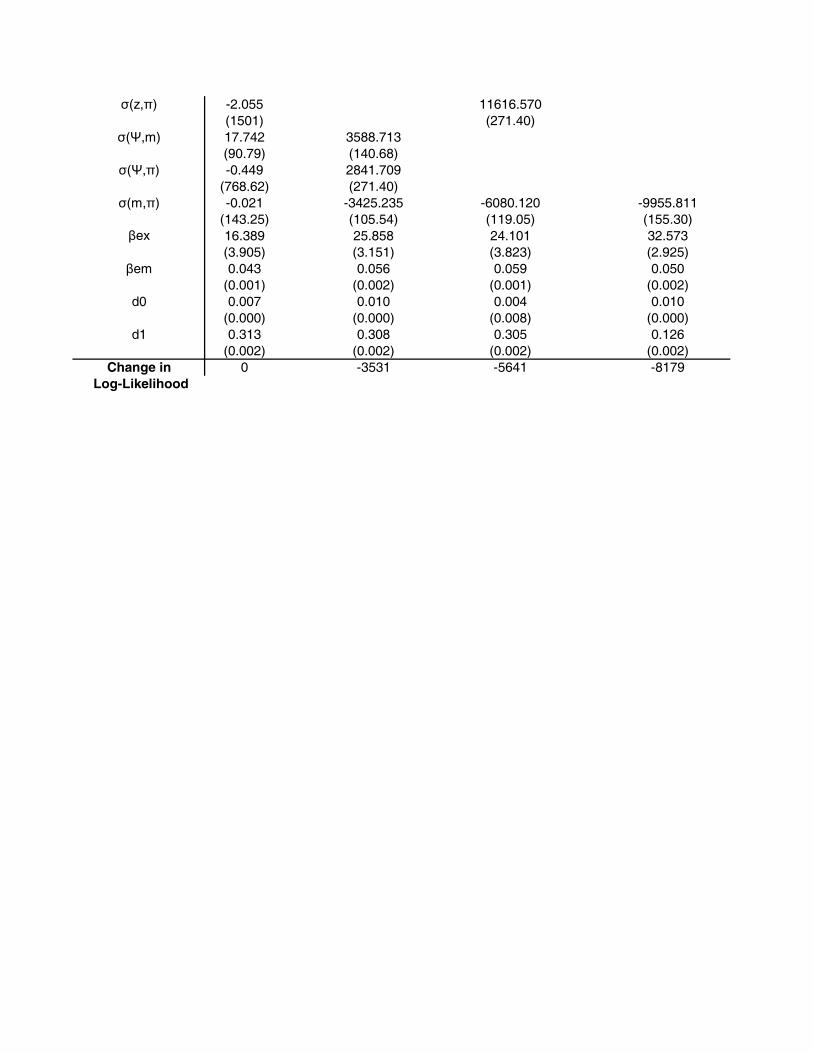
The constrained models in Table 1 produce estimates for their unconstrained

parameters which are generally in line with those of the unconstrained model. In

particular, the constrained models also produce highly persistent processes, fit a more

persistent process for expected inflation than for the real rate, and deliver negative

estimates of σmπ and, with the exception of the constant-zt model, of σxm. Finally,Table 1 reports the losses in log likelihood from imposing the constraints. These losses

are extremely large, essentially because of our auxiliary measurement equations for

the dividend yield and the conditional covariance of bond and stock returns. The

loss in log likelihood is considerably larger when we constrain inflation volatility to

be constant than when we constrain risk aversion to be constant.

3.3 Fitted state variables

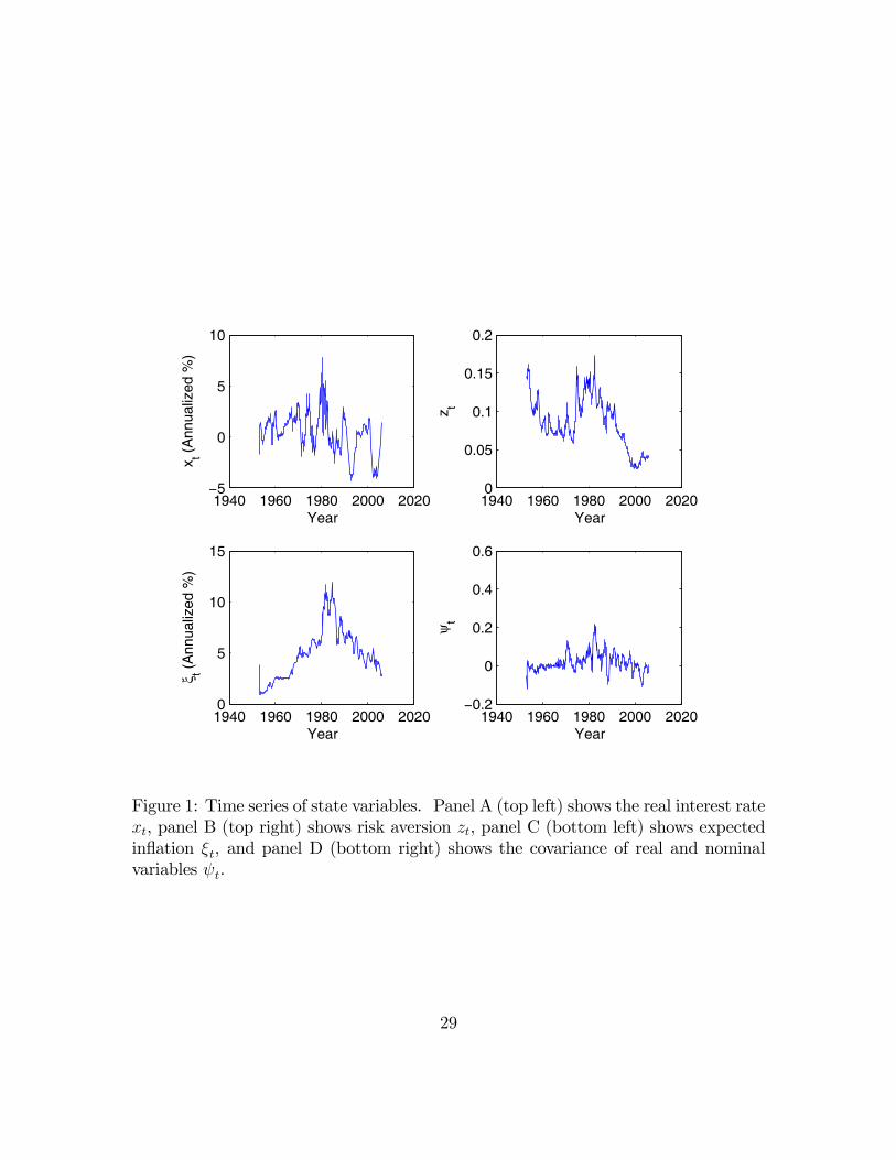
Figure 1 plots the fitted time series of the latent state variables implied by our model

estimates. Panel A in Figure 1 plots the time series of the short-term real interest

rate. Panel A shows that short-term real rates were higher on average in the first

half of our sample than in the second half, and reached a maximum of about 9.5%

in the early 1980’s. However, they appear to be more volatile in the second half of

the sample where, interestingly, we estimate the real interest rate to be significantly

negative at different points in time, particularly in the recessions of the early 1990’s

volatility of realized inflation as³μ2ψ + σ2ψ

´1/2σπ.

15

and early 2000’s. This increased real interest rate volatility is in contrast with recent

estimates of volatility in macroeconomic variables showing that growth, investment,

and inflation volatility declined in the 1980’s and 1990’s (Stock and Watson, 2002).

Panel B in Figure 1 plots the time series of zt. This is effectively a scaled version ofthe dividend yield given our assumption in equation (17) that the dividend yield is a

multiple of zt plus white noise measurement error. Consistent with our interpretationof zt as aggregate risk aversion, the model chooses the scale factor in (17) so that ztis positive everywhere.

Panel C in Figure 1 plots the time series of expected inflation. Expected inflation

exhibits a familiar hump shape over the postwar period. It was low, even negative,

in the 1950’s and 1960’s, increased during the 1970’s and reached maximum values

of about 10% in the first half of the 1980’s. Since then, it has experienced a secular

decline to about 1% at the end of the sample. The volatility of expected inflation

also shows a hump shape; its decline in the second half of the sample is consistent

with the results in Stock and Watson (2002).

Finally, Panel D in Figure 1 shows the time series of ψt. As we have noted,

this variable is identified through the covariance of stock returns and bond returns.

Panel D is to a close approximation a scaled version of the realized covariance of

stock returns and bond returns, whose time series behavior we discuss below. It is

important to note though that ψt can and does switch sign over time. Sign switches

tend to be persistent, though there are also transitory changes in sign that appear to

be related to “flight-to-quality” events in the bond and stock markets. In particular,

we estimate ψt to be slightly negative on average for most of the 1950’s and 1960’s,

positive or highly positive on average for most of 1970’s, 1980’s and the first half of

the 1990’s, and negative on average afterwards. The volatility of ψt appears to have

increased significantly in the period that started in the 1970’s. During this period,

ψt has experimented brief periods in which it was either highly positive, such as in

the early 1980’s, or highly significantly negative, such as 1987.

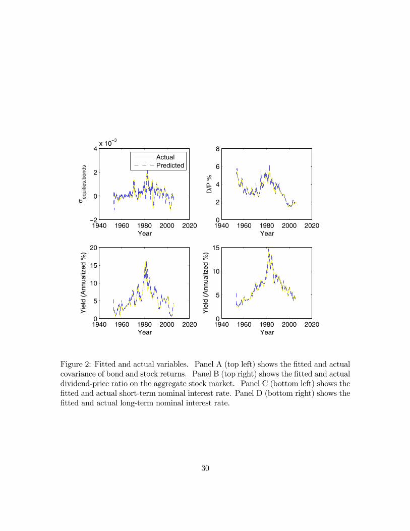
Figure 2 provides a sense of the fit of the model in the time series dimension. These

figures plot the observed and model-fitted time series of the covariance between stock

returns and bond returns, the equity dividend yield, the 3-month nominal bond yield,

and the 10-year nominal bond yield. The fitted time series of these variables almost

perfectly overlap with the observed time series, reflecting the fact that the estimation

algorithm achieves a good fit to the time series of stock and bond yields and the

stock-bond covariance.

16

Panel A in Figure 2 plots the covariance between stock returns and bond returns.

Consistent with the results in Viceira (2007), this covariance was negative in the

1950’s, relatively stable around zero in the 1960’s, and much more volatile since the

1970’s. The stock-bond covariance was highly positive in the early 1980’s, and since

then it appears to have undergone a secular decline.

The remaining panels of the figure plot relatively familiar financial time series.

The equity dividend yield, shown in Panel B, trended down throughout the 1950’s

and the 1960’s. This trend reversed during the 1970’s, when the dividend yield moved

up and reached a maximum in the early 1980’s. Since then, it has experienced a

steady decline, with only a small reversal in the early 2000’s.

Panels C and D show the time series of the observed and fitted short-term and

long-term nominal interest rates. Both short-term and nominal long-term interest

rates exhibit a pronounced hump shape, similar to the pattern we fit for expected

inflation, and shown in Panel B of Figure 1. In fact, visual inspection of the plot of

the time series of expected inflation and the time series of the 10-year nominal yield

shows that they are extremely similar. The short-term nominal rate is considerably

more volatile than the long-term nominal rate.

Table 2 reports fitted sample moments derived from these estimates, not only for

our full model but also for our three constrained models. The mean ex post real

interest rate is slightly lower than the mean ex ante real interest rate, because the

mean ex post inflation rate is slightly higher than the mean ex ante inflation rate;

our sample period had a slight preponderance of positive inflation surprises. The

model does a good job of matching the historical moments of the real interest rate and

inflation. The full model implies modest positive term premia, which are generally

lower than those implied by our restricted models, and fits the realized returns on

three-year bonds better than those models.

17

4 Implications for the Nominal Term Structure

4.1 State variables and the yield curve

Given our estimated term structure model, we can now analyze the impact of each

of our four state variables on the nominal yield curve, and thus get a sense of which

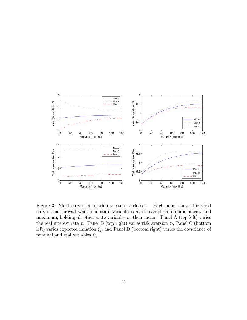
components of the curve they affect the most. To this end, we plot in Figure 3 the

zero-coupon log nominal yield curves generated by our model when one of the state

variables is at its in-sample mean, maximum, and minimum, while all other state

variables are at their in-sample means. Panels A through Panel D illustrate the yield

curves that obtain when we vary xt, zt, ξt, and ψt respectively. We plot maturities

up to 10 years, or 120 months.

The central line in each of panels in Figure 3 describes the yield curve generated

by our model when all state variables are evaluated at their in-sample mean. This

yield curve has a positive slope, with a spread between the 10-year rate and the 1-

month rate of about 110 basis points. This spread is similar to the historical average

spread in our sample period. The curve is more concave at maturities up to five years,

and considerably flatter at longer maturities. The intercept of the curve implies a

short-term nominal interest rate of about 5.4%, in line with the average short-term

nominal interest rate in our sample.

Panel A in Figure 3 shows that changes in the real interest rate move the short

end of the nominal yield curve but have almost no effect on the long end of the yield

curve; thus they alter the slope of the curve. This effect is intuitive given that we

have estimated a mean-reverting real interest rate process with a half-life of about

13 quarters. Such a process should not have a large effect on a 10-year zero-coupon

bond yield.

Panel B shows that changes in zt have almost no effect on the intercept of thenominal yield curve, but have noticeable effects on the long end of the curve. When

other state variables are at their in-sample means, nominal bonds are moderately risky

and thus their yields increase when risk aversion zt increases. This effect is much

more powerful for long-term bonds than for short-term bonds. Thus risk aversion,

like the real interest rate, alters the slope of the nominal yield curve but it does so

by moving the long end of the curve rather than the short end.

18

Panel C shows that changes in expected inflation affect short- and long-term

nominal yields almost equally, causing parallel shifts in the level of the nominal yield

curve. This effect reflects the extremely high persistence that we have estimated for

expected inflation.

The most interesting results are those shown in Panel D of Figure 3. Here we

see that changes in ψt have almost no effect on the short end of the yield curve, but

they have strong effects on both the middle of the curve and the long end. When

ψt moves from its sample mean to its sample maximum, intermediate-term bond

yields rise but long-term bond yields do not. This reflects two opposing effects of ψt

on yields. On the one hand, when ψt increases nominal bonds have higher return

volatility, and through Jensen’s Inequality this lowers the bond yield that is needed

to deliver any given expected simple return. This effect is much stronger for long-

term nominal bonds; in the terminology of the fixed-income literature, these bonds

have much greater “convexity” than short- or intermediate-term bonds. On the

other hand, when ψt increases, nominal bonds become more systematically risky and

investors demand a higher risk premium. As ψt moves from its sample mean to its

sample maximum, the two effects roughly cancel at the long end of the yield curve

but the greater risk premium dominates in the middle of the yield curve, driving

intermediate yields up relative to both short and long-term yields.

As ψt moves from its sample mean to its sample minimum, however, it moves

from slightly positive to slightly negative and there is relatively little change in the

volatility of bond returns. Thus the convexity effect is small relative to the risk

premium effect, and in panel D we see that the long end of the yield curve falls when

ψt approaches its sample minimum.

Figure 3 allows us to relate our model to traditional factor models of the term

structure of interest rates, and to provide an economic identification of those factors.

Traditional analyses distinguish a a “level” factor, a “slope” factor, and a “curvature”

factor. The first of these moves the yield curve in parallel; the second moves the short

end relative to the long end; and the third moves intermediate-term yields relative to

short and long yields. Figure 3 suggests that in our model, expected inflation is the

level factor; the short-term real interest rate and risk aversion both contribute to the

slope factor; and the covariance of nominal and real variables drives the curvature

factor and, when it is not too high, the slope factor.

19

4.2 The determinants of bond risk premia

In the previous section we saw that both risk aversion zt and the nominal-real covari-ance ψt are important determinants of long-term nominal interest rates in our model.

The reason for this is that these variables have powerful effects on risk premia. In

fact, the main determinant of nominal bond risk premia is the product ztψt.

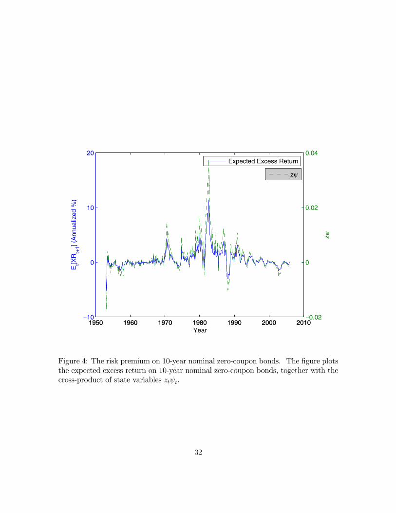
Figure 4 illustrates this by plotting the time series of the monthly risk premium on

a 10-year nominal zero-coupon bond, log Et[P$119,t+1/P

$120,t]− Et[r$1,t+1], together with

the time series of ztψt scaled to have approximately the same standard deviation. In

principle, we know from equation (16) that the nominal-bond risk premium in our

model is a linear combination of zt, ψt, their squares, and their cross-product. The

figure shows that in practice, the cross-product ztψt generates most of the variation

in the risk premium..

Our model fits the time series of postwar US bond risk premia with three periods

that broadly coincide with three distinct periods for capital market and macroeco-

nomic conditions. The first period includes most of the 1950’s and 1960’s. This was

a period of a stable tradeoff between growth and inflation and sharply declining risk

aversion, and our estimated bond risk premia reflect that; they are positive early in

the period, negative for most of the 1950’s, and close to zero in the 1960’s. The second

period includes the 1970’s and the first half of the 1980’s. This was a period of an

unstable relation between inflation and growth, a declining stock market, and increas-

ing risk aversion. Our estimated bond risk premia during this period are positive on

average, with considerable volatility. The third period runs from the mid-1980’s until

the end of our sample period. This period has been characterized by a return to stable

growth and inflation, a rising stock market, and declining risk aversion. Estimated

bond risk premia show a declining trend in both their mean and their volatility, and

become negative at the end of the sample.

Our fitted bond risk premia also exhibit short episodes where they reach extreme

positive or negative values. These episodes are related to the occurrence of extreme

economic or financial events, such as the large increases in interest rates in the early

1980’s during the Volcker period, which drove bond risk premia sharply higher, or the

stock market crash of October 1987, which produced a “flight to quality” and sharply

lower bond risk premia.

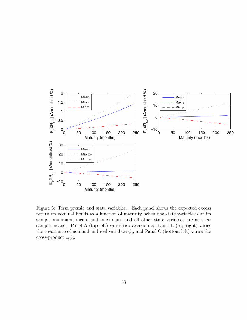
Figure 5 explores the impact of changes in zt and ψt in more detail. Panel A in the

20

figure plots bond risk premia as a function of maturity n when all state variables areat their sample mean, and zt is at its mean, minimum, and maximum values. Panel

B is identical in structure to Panel A, except that it varies ψt instead of zt. Panel Cvaries the product ztψt.

Consistent with the analysis of the impact of state variables on bond yields shown

in Figure 3, Panel A shows that zt always increases bond risk premia, and that theimpact is increasing in the maturity of the bond. However, even at a maturity of 20

years, the conditional bond risk premium evaluated at the maximum value of zt isonly slightly larger than 2% per annum. By contrast, Panel B shows that ψt has a

very pronounced effect on bond risk premia: The conditional risk premium on a 20-

year bond evaluated at the maximum value of ψt is about 15% per annum. Moreover,

conditional bond risk premia are increasingly negative as a function of maturity when

ψt is at its sample minimum. Panel C shows a similar pattern to Panel B, but the

positive risk premia at the maximum are accentuated while the negative risk premia

at the minimum are less extreme. The reason is that in our sample period, large

positive values of ψt coincided with large positive values of zt, whereas large negativevalues of ψt coincided with much smaller values of zt.

We saw in Figure 3 that the nominal-real correlation ψt influences the curvature

of the yield curve as well as its slope. Other factors in our model, such as the real

interest rate, also influence the slope of the yield curve but do not have much effect

on its curvature. Given the dominant influence of ψt on bond risk premia, illustrated

in Figure 5, the curvature of the yield curve may be a good empirical proxy for risk

premia on nominal bonds.

In fact, an empirical result of this sort has been reported by Cochrane and Pi-

azzesi (2005). Using econometric methods originally developed by Hansen and Ho-

drick (1983), and implemented in the term structure context by Stambaugh (1988),

Cochrane and Piazzesi show that a single linear combination of forward rates is a

good predictor of excess bond returns at a wide range of maturities. Interestingly,

this combination of forward rates is tent-shaped, with a peak at 3 or 4 years, imply-

ing that bond risk premia are high when intermediate-term interest rates are high

relative to both shorter-term and longer-term rates; that is, they are high when the

yield curve is strongly concave.

Table 3 reports a similar exercise to that of Cochrane and Piazzesi. Using both

our raw data and the fitted yield curves from our estimated models, we regress both

ten-year and three-year realized excess returns onto the yield spread and onto our

21

estimated optimal combination of forward rates, which we call “Tent”. These regres-

sions are fairly similar in the data and in all of our models, since all the models track

the in-sample behavior of the yield curve fairly well. Like Cochrane and Piazzesi,

we find that the tent variable produces a higher R2 statistic and stronger statisticalsignificance than does the yield spread.

Each of our models implies a different history for the expected (as opposed to the

realized) excess bond return. We regress our model-implied expected returns onto

the yield spread and the tent variable, and again find that the tent variable delivers

a better fit. The difference in fit is particularly pronounced in our full model where

both zt and ψt move over time.

Finally, we regress realized returns onto the expected excess returns implied by

each of our models. We obtain coefficients close to one for our full model, but

smaller and even in one case negative coefficients for our restricted models. This

finding strongly suggests that our full model is necessary to explain the predictability

of excess bond returns in our postwar US dataset.

5 Conclusion

In this paper we have argued that changing covariances between nominal and real

variables are of central importance in understanding the term structure of nominal

interest rates. Analyses of asset allocation traditionally assume that broad asset

classes have a stable structure of risk over time; our empirical results suggest that in

the case of nominal bonds and stocks, at least, this assumption is seriously misleading.

Our term structure model implies that the risk premia of nominal bonds have

changed over the decades, in part with movements in risk aversion that are proxied

by changes in the equity dividend yield, and in part with changes in the covariance

between inflation and the real economy. Nominal bond risk premia were particularly

high in the early 1980’s, when bonds covaried strongly with stocks and risk aversion

was high; they were negative in the early 2000’s, when bonds covaried negatively with

stocks, but at this time risk aversion was relatively low, so negative bond risk premia

were modest in magnitude.

Our model explains the finding of Cochrane and Piazzesi (2005) that a tent-shaped

linear combination of forward rates, with a peak at 3 or 4 years, predicts excess bond

22

returns at all maturities better than maturity-specific yield spreads. In our model,

the covariance between inflation and the real economy has opposing effects on longer-

term bond yields. It raises them by increasing the risk premium, but it lowers

them through a Jensen’s Inequality effect of increasing volatility. In the language

of fixed-income investors, longer-term bonds have “convexity” which becomes more

valuable when volatility is high. At the long end of the yield curve, these two

effects roughly cancel for high levels of the nominal-real covariance, whereas at the

intermediate portion of the curve, the risk premium effect dominates. Hence, the

level of intermediate yields relative to short- and long-term yields is a good proxy for

the nominal-real covariance and hence for the risk premium on nominal bonds.

The results we have presented are preliminary and this research can be extended

in a number of directions. First, we can use alternative estimation methods, such as

the Efficient Method of Moments of Gallant and Tauchen (1996), to properly handle

econometric difficulties caused by the nonlinearity of our term structure model.

Second, we can derive stock returns from primitive assumptions on the dividend

process, as in the recent literature on affine models of stock and bond pricing (Ma-

maysky 2002, Bekaert, Engstrom, and Grenadier 2004, d’Addona and Kind 2005).

Third, we can ask our model to fit a wider range of conditional second moments for

asset returns; this may require us to generalize the model to allow heteroskedasticity

in real as well as nominal variables.

Fourth, we can ask our model to fit data from the last ten years on the yields

of TIPS (Treasury inflation-protected securities) as well as the longer time series for

nominal bond yields. This additional source of information will allow us to ask,

for example, whether real bond returns have stable covariances with stock returns as

implied by our model.

Fifth, we can explore the relation between our covariance state variable ψt and the

state of monetary policy and the macroeconomy. We have suggested that a positive

ψt corresponds to an environment in which the Phillips Curve is unstable, while a

negative ψt reflects a stable Phillips Curve. It would be desirable to use data on

inflation and output more directly to explore this interpretation.

Sixth, we can enrich our description of the real interest rate. To the extent that

the short-term real interest rate is controlled by the Federal Reserve, its covariance

with the stochastic discount factor and the stock market reflects the policy rule of the

23

monetary authority. For example, the hypothesis that the Federal Reserve cuts the

real interest rate when the stock market is weak, and raises it when the stock market

is strong (the so-called “Greenspan put”) would imply a negative covariance between

xt and mt. If such policy behavior has altered over time, then this covariance too

would be time-varying rather than constant.

Finally, we can apply our model to other countries with different inflation histories.

One particularly interesting country is the UK, where inflation-indexed bonds have

been actively traded since the mid-1980’s.

24

References

Ahn, Dong-Hyun, Robert F. Dittmar, and A. Ronald Gallant, 2002, “Quadratic

Term Structure Models: Theory and Evidence”, Review of Financial Studies

15, 243—288.

Baele, Lieven, Geert Bekaert, and Koen Inghelbrecht, 2007, “The Determinants of

Stock and Bond Return Comovements”, unpublished paper, Tilburg University,

Columbia University, and Ghent University.

Barsky, Robert B., 1989, “Why Don’t the Prices of Stocks and Bonds Move To-

gether?”, American Economic Review 79, 1132—1145.

Bekaert, Geert, Eric Engstrom, and Steve Grenadier, 2004, “Stock and Bond Returns

with Moody Investors”, unpublished paper, Columbia University, University of

Michigan, and Stanford University.

Buraschi, Andrea and Alexei Jiltsov, 2007, “Habit Formation and the Term Struc-

ture of Interest Rates”, Journal of Finance, forthcoming.

Campbell, John Y., 1986, “Bond and Stock Returns in a Simple Exchange Model”,

Quarterly Journal of Economics 101, 785—804.

Campbell, John Y. and John Ammer, 1993, “What Moves the Stock and Bond

Markets? A Variance Decomposition for Long-Term Asset Returns”, Journal

of Finance 48, 3—37.

Campbell, John Y., Y. Lewis Chan, and Luis M. Viceira, 2003, “A Multivariate

Model of Strategic Asset Allocation”, Journal of Financial Economics 67, 41—

80.

Campbell, John Y. and John H. Cochrane, 1999, “By Force of Habit: A Consumption-

Based Explanation of Aggregate Stock Market Behavior”, Journal of Political

Economy 107, 205—251.

Campbell, John Y., Andrew W. Lo, and A. Craig MacKinlay, 1997, The Economet-

rics of Financial Markets, Princeton University Press, Princeton, NJ.

Campbell, John Y. and Robert J. Shiller, 1991, “Yield Spreads and Interest Rate

Movements: A Bird’s Eye View”, Review of Economic Studies 58, 495—514.

25

Campbell, John Y., Adi Sunderam, and Luis M. Viceira, 2007, “Appendix to In-

flation Bets or Deflation Hedges? The Changing Risks of Nominal Bonds”,

available online at http://kuznets.fas.harvard.edu/~campbell/papers.html.

Campbell, John Y. and Luis M. Viceira, 2001, “Who Should Buy Long-TermBonds?”,

American Economic Review 91, 99—127.

Campbell, John Y. and Luis M. Viceira, 2002, Strategic Asset Allocation: Portfolio

Choice for Long-Term Investors, Oxford University Press, New York, NY.

Campbell, John Y. and Motohiro Yogo, 2006, “Efficient Tests of Predictability in

Stock Returns”, Journal of Financial Economics 81, 27—60.

Cochrane, John H. and Monika Piazzesi, 2005, “Bond Risk Premia”, American

Economic Review 95, 138—160.

Connolly, Robert, Chris Stivers, and Licheng Sun, 2005, “Stock Market Uncertainty

and the Stock-Bond Return Relation”, Journal of Financial and Quantitative

Analysis 40, 161—194.

Constantinides, George M., 1992, “A Theory of the Nominal Term Structure of

Interest Rates”, Review of Financial Studies 5, 531—552.

Cox, John C., Jonathan E. Ingersoll, and Stephen A. Ross, 1985, “An Intertemporal

General Equilibrium Model of Asset Prices”, Econometrica 53, 363—384.

d’Addona, Stefano and Axel H. Kind, 2005, “International Stock-Bond Correlations

in a Simple Affine Asset Pricing Model”, unpublished paper, Columbia Univer-

sity and University of St. Gallen.

Dai, Qiang and Kenneth Singleton, 2002, “Expectations Puzzles, Time-Varying Risk

Premia, and Affine Models of the Term Structure”, Journal of Finance 63, 415—

442.

David, Alexander and Pietro Veronesi, 2004, “Inflation and Earnings Uncertainty

and Volatility Forecasts”, unpublished paper, Washington University and Uni-

versity of Chicago.

Engle, Robert F., 1982, “Autoregressive Conditional Heteroskedasticity with Esti-

mates of the Variance of UK Inflation”, Econometrica 50, 987—1008.

26

Fama, Eugene F., 2006, “The Behavior of Interest Rates” Review of Financial Stud-

ies 19, 359-379.

Fama, Eugene F. and Robert R. Bliss, 1987, “The Information in Long-Maturity

Forward Rates”, American Economic Review 77, 680-692.

Fama, Eugene F. and Kenneth R. French, 1989, “Business Conditions and Expected

Returns on Stocks and Bonds”, Journal of Financial Economics 25, 23—49.

Gallant, Ronald and George Tauchen, 1996, "Which Moments to Match”, Econo-

metric Theory 12, 657-681.

Gollier, Christian, 2005, “The Consumption-Based Determinants of the Term Struc-

ture of Discount Rates”, unpublished paper, University of Toulouse.

Guidolin, Massimo and Allan Timmermann, 2004, “An Econometric Model of Non-

linear Dynamics in the Joint Distribution of Stock and Bond Returns”, unpub-

lished paper.

Gurkaynak, Sack, and Wright, 2006, available online at

http://www.federalreserve.gov/pubs/feds/2006/200628.

Hansen, Lars P. and Robert J. Hodrick, 1983, “Risk Averse Speculation in the For-

ward Foreign Exchange Market: An Econometric Analysis of Linear Models”, in

J. Frenkel (ed.) Exchange Rates and International Macroeconomics, University

of Chicago Press, Chicago.

Lewellen, Jonathan, 2004, “Predicting Returns with Financial Ratios”, Journal of

Financial Economics 74, 209—235.

Mamaysky, Harry, 2002, “Market Prices of Risk and Return Predictability in a Joint

Stock-Bond Pricing Model”, Yale ICF Working Paper 02-25.

McCulloch, J. Huston and H. Kwon, 1993, “US Term Structure Data, 1947—1991”,

Working Paper 93-6, Ohio State University.

Piazzesi, Monika and Martin Schneider, 2007, “Equilibrium Yield Curves”, in D.

Acemoglu, K. Rogoff, and M. Woodford (eds.) NBER Macroeconomics Annual

2006, 317-363, MIT Press, Cambridge, MA.

27

Shiller, Robert J. and Andrea Beltratti, 1992,“Stock Prices and Bond Yields: Can

Their Comovements Be Explained in Terms of Present Value Models?”, Journal

of Monetary Economics 30, 25—46.

Stambaugh, Robert F., 1988, “The Information in Forward Rates: Implications for

Models of the Term Structure”, Journal of Financial Economics 21, 41—70..

Stambaugh, Robert F., 1999, “Predictive Regressions”, Journal of Financial Eco-

nomics 54:375-421, 1999.

Stock, James H. and Mark Watson, 2002, “Has the Business Cycle Change and-

Why?,” in M. Gertler and K. Rogoff (eds.) NBER Macroeconomics Annual:

2002, MIT Press, Cambridge, MA.

Vasicek, Oldrich, 1977, “An Equilibrium Characterization of the Term Structure”,

Journal of Financial Economics 5, 177—188.

Viceira, Luis M., 2007, “Bond Risk, Bond Return Volatility, and the Term Structure

of Interest Rates”, unpublished paper, Harvard Business School.

Wachter, Jessica A., 2006, “A Consumption-Based Model of the Term Structure of

Interest Rates”, Journal of Financial Economics 79, 365—399.

28

1940 1960 1980 2000 2020−5

0

5

10

Year

x t (A

nnua

lized

%)

1940 1960 1980 2000 20200

0.05

0.1

0.15

0.2

Year

z t

1940 1960 1980 2000 20200

5

10

15

Year

ξ t (A

nnua

lized

%)

1940 1960 1980 2000 2020−0.2

0

0.2

0.4

0.6

Year

ψt

Figure 1: Time series of state variables. Panel A (top left) shows the real interest rate

xt, panel B (top right) shows risk aversion zt, panel C (bottom left) shows expected

inflation ξt, and panel D (bottom right) shows the covariance of real and nominal

variables ψt.

29

1940 1960 1980 2000 2020−2

0

2

4x 10

−3

Year

σ equi

ties,

bond

s

ActualPredicted

1940 1960 1980 2000 20200

2

4

6

8

Year

D/P

%

1940 1960 1980 2000 20200

5

10

15

20

Year

Yie

ld (

Ann

ualiz

ed %

)

1940 1960 1980 2000 20200

5

10

15

Year

Yie

ld (

Ann

ualiz

ed %

)

Figure 2: Fitted and actual variables. Panel A (top left) shows the fitted and actual

covariance of bond and stock returns. Panel B (top right) shows the fitted and actual

dividend-price ratio on the aggregate stock market. Panel C (bottom left) shows the

fitted and actual short-term nominal interest rate. Panel D (bottom right) shows the

fitted and actual long-term nominal interest rate.

30

0 20 40 60 80 100 1200

5

10

15

Maturity (months)

Yie

ld (

Ann

ualiz

ed %

)

MeanMax xMin x

0 20 40 60 80 100 1205

5.5

6

6.5

7

Maturity (months)Y

ield

(A

nnua

lized

%)

Mean

Max z

Min z

0 20 40 60 80 100 1200

5

10

15

Maturity (months)

Yie

ld (

Ann

ualiz

ed %

)

MeanMax ξMin ξ

0 20 40 60 80 100 1205

5.5

6

6.5

7

Maturity (months)

Yie

ld (

Ann

ualiz

ed %

)

Mean

Max ψMin ψ

Figure 3: Yield curves in relation to state variables. Each panel shows the yield

curves that prevail when one state variable is at its sample minimum, mean, and

maximum, holding all other state variables at their mean. Panel A (top left) varies

the real interest rate xt, Panel B (top right) varies risk aversion zt, Panel C (bottomleft) varies expected inflation ξt, and Panel D (bottom right) varies the covariance ofnominal and real variables ψt.

31

1950 1960 1970 1980 1990 2000 2010−10

0

10

20

Year

Et[X

Rt+

1] (A

nnua

lized

%)

Expected Excess Return

1950 1960 1970 1980 1990 2000 2010−0.02

0

0.02

0.04

zψ

zψ

Figure 4: The risk premium on 10-year nominal zero-coupon bonds. The figure plots

the expected excess return on 10-year nominal zero-coupon bonds, together with the

cross-product of state variables ztψt.

32

0 50 100 150 200 2500

0.5

1

1.5

2

Maturity (months)

Et[X

Rt+

1] (A

nnua

lized

%)

Mean

Max z

Min z

0 50 100 150 200 250−10

0

10

20

Maturity (months)

Et[X

Rt+

1] (A

nnua

lized

%)

Mean

Max ψMin ψ

0 50 100 150 200 250−10

0

10

20

30

Maturity (months)

Et[X

Rt+

1] (A

nnua

lized

%)

Mean

Max zψMin zψ

Figure 5: Term premia and state variables. Each panel shows the expected excess

return on nominal bonds as a function of maturity, when one state variable is at its

sample minimum, mean, and maximum, and all other state variables are at their

sample means. Panel A (top left) varies risk aversion zt, Panel B (top right) variesthe covariance of nominal and real variables ψt, and Panel C (bottom left) varies the

cross-product ztψt.

33

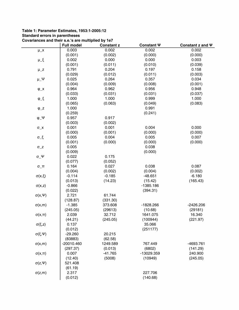
Table 1: Parameter Estimates, 1953:1-2005:12Standard errors in parenthesesCovariances and their s.e.'s are multiplied by 1e7

Full model Constant z Constant Ψ Constant z and Ψμ_x 0.003 0.002 0.002 0.002

(0.001) (0.002) (0.000) (0.000)μ_ξ 0.002 0.000 0.000 0.003

(0.001) (0.011) (0.010) (0.039)μ_z 0.791 0.204 0.197 0.158

(0.029) (0.012) (0.011) (0.003)μ_Ψ 0.025 0.264 0.357 0.034

(0.004) (0.009) (0.008) (0.001)φ_x 0.964 0.962 0.956 0.948

(0.033) (0.031) (0.031) (0.037)φ_ξ 1.000 1.000 0.999 1.000

(0.065) (0.063) (0.049) (0.083)φ_z 1.000 0.991

(0.259) (0.241)φ_Ψ 0.957 0.917

(0.003) (0.002)σ_x 0.001 0.001 0.004 0.000

(0.000) (0.001) (0.000) (0.000)σ_ξ 0.005 0.004 0.005 0.007

(0.001) (0.000) (0.000) (0.000)σ_z 0.005 0.038

(0.009) (0.000)σ_Ψ 0.022 0.175

(0.077) (0.052)σ_π 0.164 0.027 0.038 0.087

(0.004) (0.002) (0.004) (0.002)σ(x,ξ) -0.114 -0.185 -48.651 -6.180

(0.013) (14.23) (15.42) (165.43)σ(x,z) -0.866 -1385.186

(0.022) (394.31)σ(x,Ψ) 2.721 61.744

(128.87) (331.30)σ(x,m) -1.385 373.608 -1828.266 -2426.206

(245.05) (29613) (10.68) (29181)σ(x,π) 2.039 32.712 1641.075 16.340

(44.21) (245.05) (100944) (221.97)σ(ξ,z) 0.137 35.066

(0.012) (251177)σ(ξ,Ψ) -29.260 20.215

(83883) (62.58)σ(x,m) -20010.460 1249.589 767.449 -4693.761

(297.37) (0.013) (6802) (141.29)σ(x,π) 0.007 -41.765 -13029.359 240.900

(12.40) (5008) (10949) (245.05)σ(z,Ψ) 521.408

(61.19)σ(z,m) 2.317 227.706

(0.012) (140.68)

σ(z,π) -2.055 11616.570(1501) (271.40)

σ(Ψ,m) 17.742 3588.713(90.79) (140.68)

σ(Ψ,π) -0.449 2841.709(768.62) (271.40)

σ(m,π) -0.021 -3425.235 -6080.120 -9955.811(143.25) (105.54) (119.05) (155.30)

βex 16.389 25.858 24.101 32.573(3.905) (3.151) (3.823) (2.925)

βem 0.043 0.056 0.059 0.050(0.001) (0.002) (0.001) (0.002)

d0 0.007 0.010 0.004 0.010(0.000) (0.000) (0.008) (0.000)

d1 0.313 0.308 0.305 0.126(0.002) (0.002) (0.002) (0.002)

Change in 0 -3531 -5641 -8179 Log-Likelihood

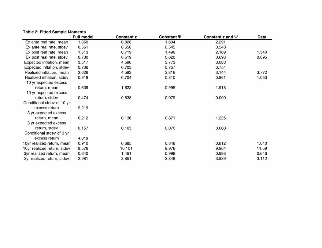
Table 2: Fitted Sample MomentsFull model Constant z Constant Ψ Constant z and Ψ Data

Ex ante real rate, mean 1.850 0.828 1.604 2.291Ex ante real rate, stdev 0.561 0.558 0.545 0.543Ex post real rate, mean 1.513 0.719 1.496 2.169 1.540Ex post real rate, stdev 0.730 0.519 0.620 0.698 0.895

Expected inflation, mean 3.517 4.596 3.773 3.083Expected inflation, stdev 0.706 0.703 0.757 0.754Realized inflation, mean 3.626 4.593 3.816 3.144 3.772Realized inflation, stdev 0.918 0.704 0.810 0.861 1.05310 yr expected excess

return, mean 0.639 1.623 0.995 1.91810 yr expected excess

return, stdev 0.474 0.838 0.079 0.000Conditional stdev of 10 yr

excess return 9.2193 yr expected excess

return, mean 0.212 0.136 0.871 1.2253 yr expected excess

return, stdev 0.157 0.165 0.070 0.000Conditional stdev of 3 yr

excess return 4.01910yr realized return, mean 0.910 0.685 0.848 0.812 1.04010yr realized return, stdev 9.576 10.101 9.976 9.964 11.593yr realized return, mean 0.640 1.461 0.998 0.998 0.6463yr realized return, stdev 2.981 3.851 3.848 3.839 3.112

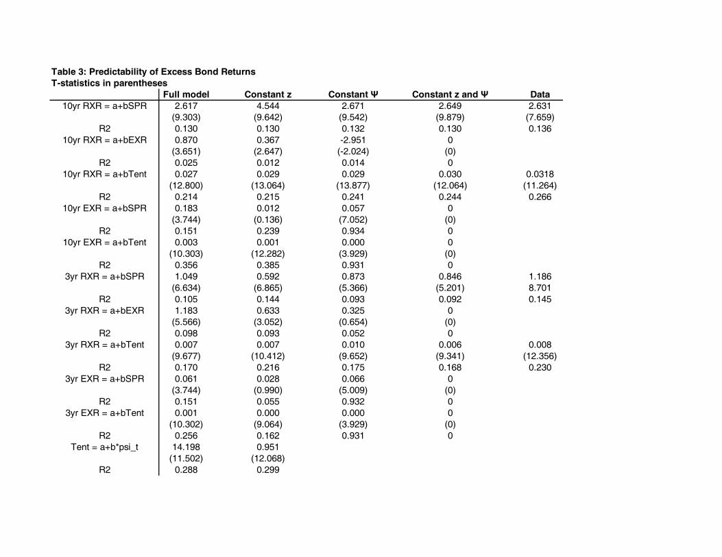
Table 3: Predictability of Excess Bond ReturnsT-statistics in parentheses

Full model Constant z Constant Ψ Constant z and Ψ Data10yr RXR = a+bSPR 2.617 4.544 2.671 2.649 2.631

(9.303) (9.642) (9.542) (9.879) (7.659)R2 0.130 0.130 0.132 0.130 0.136

10yr RXR = a+bEXR 0.870 0.367 -2.951 0(3.651) (2.647) (-2.024) (0)

R2 0.025 0.012 0.014 010yr RXR = a+bTent 0.027 0.029 0.029 0.030 0.0318

(12.800) (13.064) (13.877) (12.064) (11.264)R2 0.214 0.215 0.241 0.244 0.266

10yr EXR = a+bSPR 0.183 0.012 0.057 0(3.744) (0.136) (7.052) (0)

R2 0.151 0.239 0.934 010yr EXR = a+bTent 0.003 0.001 0.000 0

(10.303) (12.282) (3.929) (0)R2 0.356 0.385 0.931 0

3yr RXR = a+bSPR 1.049 0.592 0.873 0.846 1.186(6.634) (6.865) (5.366) (5.201) 8.701

R2 0.105 0.144 0.093 0.092 0.1453yr RXR = a+bEXR 1.183 0.633 0.325 0

(5.566) (3.052) (0.654) (0)R2 0.098 0.093 0.052 0

3yr RXR = a+bTent 0.007 0.007 0.010 0.006 0.008(9.677) (10.412) (9.652) (9.341) (12.356)

R2 0.170 0.216 0.175 0.168 0.2303yr EXR = a+bSPR 0.061 0.028 0.066 0

(3.744) (0.990) (5.009) (0)R2 0.151 0.055 0.932 0

3yr EXR = a+bTent 0.001 0.000 0.000 0(10.302) (9.064) (3.929) (0)

R2 0.256 0.162 0.931 0Tent = a+b*psi_t 14.198 0.951

(11.502) (12.068)R2 0.288 0.299