Economic Modelling 30 (2013) 900–910

Contents lists available at SciVerse ScienceDirect

Economic Modelling

j ourna l homepage: www.e lsev ie r .com/ locate /ecmod

Income–happiness paradox in Australia: Testing the theories of adaptationand social comparison☆

Satya Paul ⁎, Daniel GuilbertUniversity of Western Sydney, Penrith South DC, NSW 1797, Australia

☆ We are grateful to an anonymous referee for useful cthis paper. This paper uses unit record data from the HDynamics in Australia (HILDA) Survey. The HILDA Projeby the Australian Government Department of Families,and Indigenous Affairs (FaHCSIA) and is managed bApplied Economic and Social Research (Melbourne Instreported in this paper, however, are those of the authorto either FaHCSIA or the Melbourne Institute.⁎ Corresponding author at: School of Economics and

Room EDG 136, University of Western Sydney, LockedNSW 1797, Australia. Tel.: +61 2 96859352 (Office), +

E-mail address: s.paul@uws.edu.au (S. Paul).

0264-9993/$ – see front matter © 2012 Elsevier B.V. Allhttp://dx.doi.org/10.1016/j.econmod.2012.08.034

a b s t r a c t

a r t i c l e i n f o

Article history:Accepted 6 August 2012

JEL classification:D3D6I3

Keywords:Life satisfactionAdaptationComparison incomeEasterlin paradox

This paper investigates whether the theories of adaptation and social comparison can explain the income–happiness puzzle (Easterlin Paradox) in Australia. Alternative specifications of happiness model that incorpo-rate adaption, comparison incomes and other relevant variables are estimated using the panel data from thefive waves (2001–2005) of the Household Income and Labour Dynamics in Australia (HILDA) surveys. Thestatistical tests provide no support for the adaptation effect on happiness. However, we find strong supportfor the theory of social comparison as an explanation for the happiness paradox. An increase in peer groupincome hurts the poor more than the rich, suggesting that a redistribution of income is likely to enhancethe overall wellbeing of society. A sensitivity analysis is conducted to check the robustness of results.

© 2012 Elsevier B.V. All rights reserved.

1. Introduction

Economic theory suggests that a higher income allows an insatiableconsumer to reach a higher indifference curve and achieve a greaterlevel of utility. However, the existing empirical studies of the relation-ship between utility (self reported happiness) and income report para-doxical results. At a point of time, people with higher levels of incomeare happier than those with lower income. Over the time, happinessdoes not increase when a country's income increases. The point oftime statement is based on the cross-sectional comparison of averagehappiness and income within and between countries; the time seriesstatement relates happiness with economic growth in a country.Easterlin (1974) is the first to report this paradox based on his analysisof happiness data from the yearly surveys for the United States. Hereports that the rich people are happier than the poor within the USin a given year. Yet since World War II, the happiness responses areflat in the face of considerable increases in real average income.

omments on an earlier draft ofousehold, Income and Labourct was initiated and is fundedHousing, Community Servicesy the Melbourne Institute ofitute). The findings and viewss and should not be attributed

Finance, Parramatta Campus,Bag 1797, Penrith South DC,61 404816145 (Mob).

rights reserved.

This happiness paradox, popularly known as the “Easterlin paradox,”is not specifically a US phenomenon. A similar picture is observed in anumber of other developed countries including France, Germany,Japan and the United Kingdom at different periods of time (Easterlin,1995; Inglehart and Klingemann, 2000; Blanchflower and Oswald,2004; Clark et al., 2008; Easterlin andAngelescu, 2009). In Japan, despitea five-fold increase in real per capita income between 1958 and 1987,mean subjective wellbeing (happiness) has not budged.

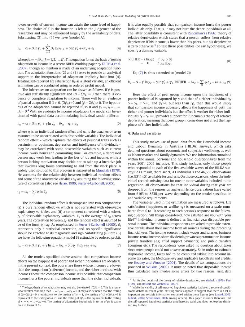
In Australia, the mean values of individual real income and happi-ness scores obtained from the Household Income and Labour Dynamicsin Australia (HILDA) surveys reveal that while the level of income hasgrown, reported happiness has fallen slightly during the period 2001–2005 (Table 1 and Fig. 1). The aim of this paper is to explain thisobserved income–happiness puzzle.1

To date, there appears to have been no attempt to explain theincome–happiness paradox in Australia. The existing Australian stud-ies of happiness are concerned with the effects of income, wealth andother relevant variables such as education, unemployment and age onwell-being and ill-being using survey data for one or few years. Forinstance, Headey and Wooden (2004) used HILDA survey data for2002 to investigate the determinant of well-being and ill-being inAustralia. The well-being of an individual is measured in terms oftwo separate variables, life satisfaction and financial satisfaction,whereas ill-being is measured in terms of mental health and financialstress. The study reveals that the effect of wealth on life and financial

1 The terms ‘Easterlin paradox’, ‘happiness paradox’ and ‘income-happiness puzzle’are used interchangeably throughout this paper.

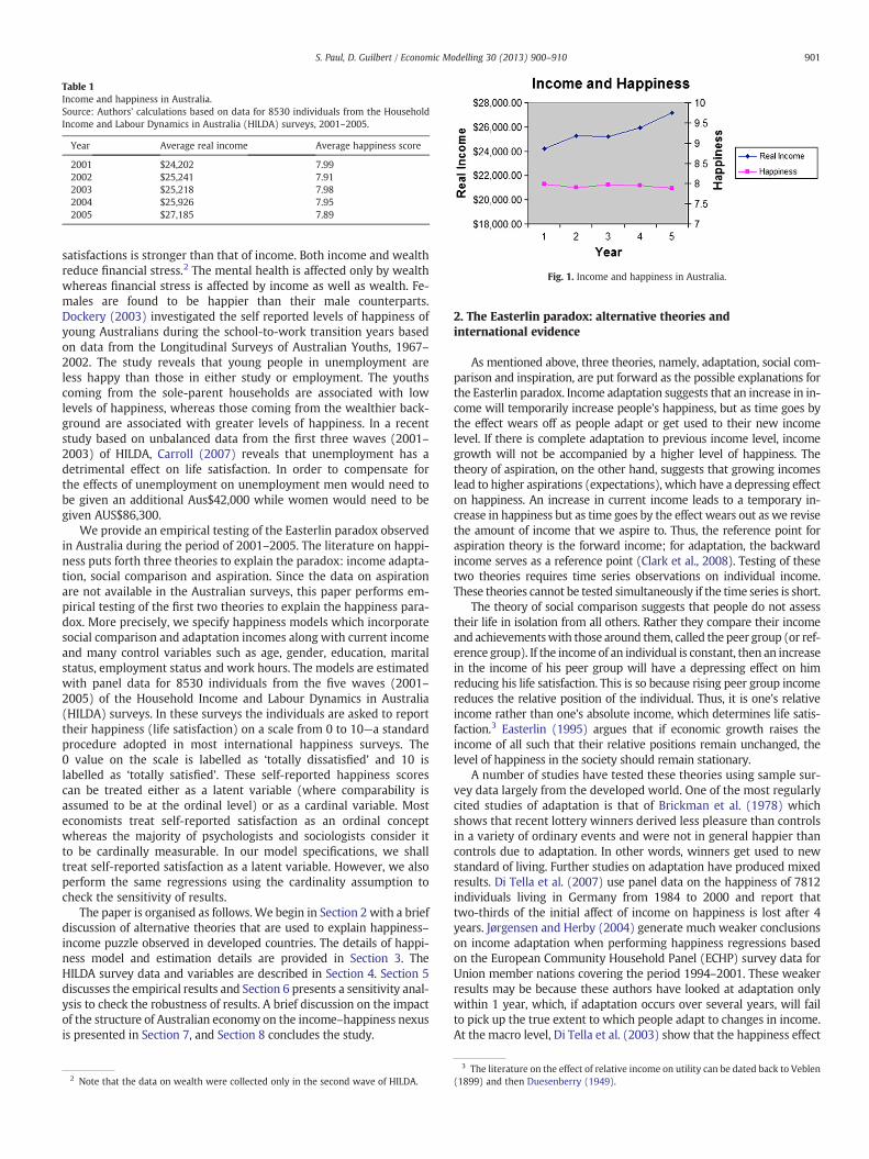
Fig. 1. Income and happiness in Australia.

Table 1Income and happiness in Australia.Source: Authors’ calculations based on data for 8530 individuals from the HouseholdIncome and Labour Dynamics in Australia (HILDA) surveys, 2001–2005.

Year Average real income Average happiness score

2001 $24,202 7.992002 $25,241 7.912003 $25,218 7.982004 $25,926 7.952005 $27,185 7.89

901S. Paul, D. Guilbert / Economic Modelling 30 (2013) 900–910

satisfactions is stronger than that of income. Both income and wealthreduce financial stress.2 The mental health is affected only by wealthwhereas financial stress is affected by income as well as wealth. Fe-males are found to be happier than their male counterparts.Dockery (2003) investigated the self reported levels of happiness ofyoung Australians during the school-to-work transition years basedon data from the Longitudinal Surveys of Australian Youths, 1967–2002. The study reveals that young people in unemployment areless happy than those in either study or employment. The youthscoming from the sole-parent households are associated with lowlevels of happiness, whereas those coming from the wealthier back-ground are associated with greater levels of happiness. In a recentstudy based on unbalanced data from the first three waves (2001–2003) of HILDA, Carroll (2007) reveals that unemployment has adetrimental effect on life satisfaction. In order to compensate forthe effects of unemployment on unemployment men would need tobe given an additional Aus$42,000 while women would need to begiven AUS$86,300.

We provide an empirical testing of the Easterlin paradox observedin Australia during the period of 2001–2005. The literature on happi-ness puts forth three theories to explain the paradox: income adapta-tion, social comparison and aspiration. Since the data on aspirationare not available in the Australian surveys, this paper performs em-pirical testing of the first two theories to explain the happiness para-dox. More precisely, we specify happiness models which incorporatesocial comparison and adaptation incomes along with current incomeand many control variables such as age, gender, education, maritalstatus, employment status and work hours. The models are estimatedwith panel data for 8530 individuals from the five waves (2001–2005) of the Household Income and Labour Dynamics in Australia(HILDA) surveys. In these surveys the individuals are asked to reporttheir happiness (life satisfaction) on a scale from 0 to 10—a standardprocedure adopted in most international happiness surveys. The0 value on the scale is labelled as ‘totally dissatisfied’ and 10 islabelled as ‘totally satisfied’. These self-reported happiness scorescan be treated either as a latent variable (where comparability isassumed to be at the ordinal level) or as a cardinal variable. Mosteconomists treat self-reported satisfaction as an ordinal conceptwhereas the majority of psychologists and sociologists consider itto be cardinally measurable. In our model specifications, we shalltreat self-reported satisfaction as a latent variable. However, we alsoperform the same regressions using the cardinality assumption tocheck the sensitivity of results.

The paper is organised as follows.We begin in Section 2 with a briefdiscussion of alternative theories that are used to explain happiness–income puzzle observed in developed countries. The details of happi-ness model and estimation details are provided in Section 3. TheHILDA survey data and variables are described in Section 4. Section 5discusses the empirical results and Section 6 presents a sensitivity anal-ysis to check the robustness of results. A brief discussion on the impactof the structure of Australian economy on the income–happiness nexusis presented in Section 7, and Section 8 concludes the study.

2 Note that the data on wealth were collected only in the second wave of HILDA.

2. The Easterlin paradox: alternative theories andinternational evidence

As mentioned above, three theories, namely, adaptation, social com-parison and inspiration, are put forward as the possible explanations forthe Easterlin paradox. Income adaptation suggests that an increase in in-come will temporarily increase people's happiness, but as time goes bythe effect wears off as people adapt or get used to their new incomelevel. If there is complete adaptation to previous income level, incomegrowth will not be accompanied by a higher level of happiness. Thetheory of aspiration, on the other hand, suggests that growing incomeslead to higher aspirations (expectations), which have a depressing effecton happiness. An increase in current income leads to a temporary in-crease in happiness but as time goes by the effect wears out as we revisethe amount of income that we aspire to. Thus, the reference point foraspiration theory is the forward income; for adaptation, the backwardincome serves as a reference point (Clark et al., 2008). Testing of thesetwo theories requires time series observations on individual income.These theories cannot be tested simultaneously if the time series is short.

The theory of social comparison suggests that people do not assesstheir life in isolation from all others. Rather they compare their incomeand achievementswith those around them, called the peer group (or ref-erence group). If the income of an individual is constant, then an increasein the income of his peer group will have a depressing effect on himreducing his life satisfaction. This is so because rising peer group incomereduces the relative position of the individual. Thus, it is one's relativeincome rather than one's absolute income, which determines life satis-faction.3 Easterlin (1995) argues that if economic growth raises theincome of all such that their relative positions remain unchanged, thelevel of happiness in the society should remain stationary.

A number of studies have tested these theories using sample sur-vey data largely from the developed world. One of the most regularlycited studies of adaptation is that of Brickman et al. (1978) whichshows that recent lottery winners derived less pleasure than controlsin a variety of ordinary events and were not in general happier thancontrols due to adaptation. In other words, winners get used to newstandard of living. Further studies on adaptation have produced mixedresults. Di Tella et al. (2007) use panel data on the happiness of 7812individuals living in Germany from 1984 to 2000 and report thattwo-thirds of the initial affect of income on happiness is lost after 4years. Jørgensen and Herby (2004) generate much weaker conclusionson income adaptation when performing happiness regressions basedon the European Community Household Panel (ECHP) survey data forUnion member nations covering the period 1994–2001. These weakerresults may be because these authors have looked at adaptation onlywithin 1 year, which, if adaptation occurs over several years, will failto pick up the true extent to which people adapt to changes in income.At the macro level, Di Tella et al. (2003) show that the happiness effect

3 The literature on the effect of relative income on utility can be dated back to Veblen(1899) and then Duesenberry (1949).

902 S. Paul, D. Guilbert / Economic Modelling 30 (2013) 900–910

of an increase in GDP per capita tends to disappear after 2 years in 12OECD countries. These mixed results may be due to differences in dataor adaptation period, or alternatively they could indicate that somecountries adapt to higher incomes while others do not.

Studies that have investigated the role of aspirations in explainingthe happiness paradox are few. In a survey conducted in Switzerlandbetween 1992 and 1994, people were asked to state the level ofincome that they consider ‘sufficient’, given their circumstances andexpectations. Assuming that ‘sufficient’ income might be correlatedwith true aspiration level, Stutzer (2004) estimated happiness regres-sions incorporating ‘sufficient’ income as a proxy for aspirationincome. The results revealed that people's subjective wellbeing isnegatively affected by their aspiration level in Switzerland. A similarresult is reported by Stutzer and Frey (2004) based on data fromthe German Socio-Economic Panel. This study also measures aspira-tions by the income which is evaluated as ‘sufficient’.

The effect of social comparison on happiness is explored by introduc-ing the mean income of the peer (reference) group, called the compari-son income, into the regression model. A negative and significantcoefficient for comparison income would mean that an increase in peergroup income reduces the happiness of an individual. Importantamongst the studies that have found support for the social comparisonhypothesis using this approach, or an approach very similar, includeClark and Oswald (1996) for Britain; Neumark and Postlewaite (1998)and McBride (2001) for the US; Jørgensen and Herby (2004) for severalEuropean nations; Ferrer-i-Carbonell (2005) for Germany; and Stutzer(2004) for Switzerland. One of the few exceptions is Senik (2004), whofinds that people in Russia are happier when their peers are earninghigher incomes. Senik (2004) explains this unusualfinding by suggestingthat in Russia's unstable economy, people use others’ incomes whenforming their own income expectations for the future.

While the investigation into the effect of comparison income on hap-piness can be carried out with cross-section income data for 1 year, mostof these studies have used panel data to achieve efficiency in estimation.Some researchers have used the experimental surveys to investigate theeffect of social comparison on subjective wellbeing. For instance, in anexperimental study conducted at the Harvard University in 1995,Solnick and Hemenway (1998) report that approximately 50% of the re-spondents preferred a world in which they had half the real purchasingpower, as long as their relative income position is high. Similarly, the re-sults of an experiment conducted by Miles and Rossi (2007) at the Uni-versity of Vigo, between September and November 2004 reveal thatchanges in an individual's relative position affects his subjectivewellbeing. In particular, learning that one's wage is below his referencegroup is negatively correlated with subjective wellbeing. The data fromsuch experimental surveys, though useful, may not reveal how peopletruly respond to events and changes in their everyday lives. It is for thisreason that most researchers have preferred to use large household sur-veys containing questions about income levels and subjective wellbeing.

The identification of one or more theories that could explain happi-ness paradox is of importance for public policy. Social comparison impliesthat there exists a negative externality to income generating activities.The gain in happiness to the rich is accompanied by a loss of happinessto thosewho are poor. The standard economic argumentwould then sug-gest that income generating activities should be taxed to internalise suchexternalities. The adaption and inspiration do not have such straightfor-ward policy implications. The idea that people may adapt to incomechanges raises questions for policymakers only to the extent that peoplefail to accurately forecast this adaptation when making important lifedecisions. For example, if people adapt more to an increase in incomethan they do to other positive life experiences (e.g. marriage, volunteerwork etc.), and if they fail to anticipate this adaptation, then they arelikely to devote too much effort to the pursuit of income and not enougheffort to objectives in other domains of life. At its most basic level, thiscould imply that policymakers should adjust the marginal incentives as-sociatedwith various life pursuits e.g. by taxing those activities for which

adaptation is quick and absolute (complete), and subsidising or pro-moting those activities for which adaptation is slow or incomplete.The relevance of aspirations would suggest that there may be somemerit in policymakers giving less attention to the pursuit of economicaspirations, andmore attention to other pursuit of other life aspirationssuch as good health, education, honesty and truthfulness.

3. The model and estimation

The traditional utility theory assumes that utility is an increasingfunction of income, which is at odds with the Easterlin paradox. Toaccount for the paradox, the utility function is formulated to incorpo-rate adaptation and social comparison variables as

hit ¼ α þ A λ; yið Þ þ γ ln y�it þ δxit þ εit ð1Þ

where hit is the self reported level of happiness (as a proxy for utility)of the ith individual, A(λ, yi) is the adaptation function, yit* is the meanincome of the peer group which serves as a comparison income andxit is a vector of control variables such as age, education, gender, mar-ital status, employment status, number of hours worked, volunteerwork, commuting time etc. εit is an error term subsuming the effectsof unquantifiable variables and inaccuracy in reporting life satisfac-tion (for example, my 4 could be your 5 and vice versa).

Following Layard (2005, p. 252), the adaptation function can bespecified as:

A λ; yið Þ ¼ β ln yit � λ ln yit�1ð Þ ð2Þ

where λ is an adaptation parameter and yit and yit − 1 are the currentand previous years’ incomes. β is a parameter expected to be positive.For complete adaptation λ = 1 which suggests that to remain at thesame level of happiness, current income growth must match incomegrowth from the previous year. For partial adaptability 0 b λ b 1,which implies that income growth can slow down without adverselyaffecting one's happiness level. There will be no adaptation to incomeif λ = 0 implying that to remain at the same level of happiness, noincome growth is required. In this situation an increase in incomeshould lead to a higher level of happiness.

The adaptation function (2) assumes that people adapt to incomegrowth from the previous year, i.e. adaptation is completed within 1year. This may be a very restrictive and stringent assumption. Ratherthan adapting to income growth achieved in the previous year, peo-ple may adapt to average growth of income achieved over the previ-ous few years. Such a possibility may not be ruled out if incomesfluctuate during these years. A generalised adaptation function thataccommodates this may be specified as follows.

A λ; yi;Kð Þ ¼ β ln yit �XKk¼1

λk ln yit�k

!

¼ β ln yit � ln ∏K

k¼1yλkit�k

!¼ β ln yit � ln G λ; yi;Kð Þð Þ

ð3Þ

Note that G(λ,yi,K) is the weighted geometric mean income(WGMI) for λτ = 1, where λ is a vector of adaptation parametersand τ is a vector of unit values. For λτ b 1, G(λ,yi,K) is the weightedgeometric sum of K period incomes (WGSI). For λ1=λ2=…=λK=0, G(·) takes unit value implying no adaptation to income. For com-plete adaptation λτ=1, which implies that to remain at the samelevel of happiness, current income must increase at the rate atwhich the WGMI has grown. For partial adaptation λτb1, which sug-gests that to remain at the same level of happiness, current incomemust grow at the rate at which the WGSI has grown. Note thatWGSIbWGMI. Hence in the case of partial adaptability, a somewhat

5 For further details of the theory of relative deprivation, see Yitzhaki (1979), Paul

903S. Paul, D. Guilbert / Economic Modelling 30 (2013) 900–910

lower growth of current income can attain the same level of happi-ness. The choice of K in the function is left to the judgement of theresearcher and may be influenced largely by the availability of data.Substituting (3) into (1) we have (model A):

hit ¼ α þ β ln yit þXKk¼1

βk ln yit�k þ γ ln y�it þ δxit þ εit ð4Þ

whereβk=−βλk (k=1, 2,…,K). This equation forms the basis of testingadaptation to income in a recent NBER Working paper by Di Tella et al.(2007), though no mention is made of an underlying adaptation func-tion. The adaptation functions (2) and (3) serve to provide an analyticalsupport to the interpretation of adaptation implicitly built into (4).Treating self-reported life satisfaction hit as a latent variable, an efficientestimation can be conducted using an ordered probit model.

The inferences on adaptation can be drawn as follows. If β is pos-itive and statistically significant and (β+Σβk)=0 then there is evi-dence of complete adaptation to income. There will be an evidenceof partial adaptation if β > 0, (Σβk)b0 and (β+Σβk)>0. The hypoth-esis of no adaptation cannot be rejected if β>0 and β1=β2=…=βk=0.4 With no evidence to income adaptation, the model can be es-timated with panel data accommodating individual random effects:

hit ¼ α þ β ln yit þ γ ln y�it þ δxit þ ηi þ uit ð5Þ

where ηi is an individual random effect and uit is the usual error termassumed to be uncorrelated with observable variables. The individualrandom effect – which captures the effects of personal traits such aspessimism or optimism, depression and intelligence of individuals –

may be correlated with some observable variables such as currentincome, work hours and commuting time. For example, a depressedperson may work less leading to the loss of job and income, while aperson lacking motivation may decide not to take up a lucrative jobthat involves long hours commuting to and from the work place. Awidely used solution to this problem is suggested in Mundlak (1978).He accounts for the relationship between individual random effectsand some of the observable variables by assuming the following struc-ture of correlation (also see Hsiao, 1986; Ferrer-i-Carbonell, 2005).

ηi ¼ ωi þ∑jϕj ln z�ji ð6Þ

The individual random effect is decomposed into two components:(i) a pure random effect, ωi which is not correlated with observableexplanatory variables, and (ii) a component correlated with a subset,zji of observable explanatory variables. �zji is the average of zji acrossyears. The correlation between �zji and the random effect is assumed tobe of the form ϕjlnzji. As emphasised in Ferrer-i-Carbonell (2005), ϕj

represents only a statistical correction, and no specific significanceshould be attached to its magnitude and sign. Substituting (6) into (5)we have the following equation (model B) estimable by ordered probit.

hit ¼ α þ β ln yit þ γ ln y�it þ δxit þ∑jϕj ln �zjiþωi þ uit ð7Þ

All the models specified above assume that comparison incomeeffects on the happiness of poorer and richer individuals are identical.In the present context, the poorer are those whose incomes are lowerthan the comparison (reference) income, and the richer are thosewithincomes above the comparison income. It is possible that comparisonincome hurts the poorer individuals more than the richer individuals.

4 The hypothesis of no adaptation may not also be rejected if Σβk=0. This is a some-what weaker condition than β1=β2=…=βK=0. It may also be noted that the testingof (β+Σβk)=0 is equivalent to the testing of λτ=1, the testing of (β+Σβk)>0 isequivalent to the testing of λτb1, and the testing of Σβk=0 is equivalent to the testingof λ1=λ2=…=λK=0. The testing of adaptation hypothesis in terms of βs is easierthan in terms of λs.

It is also equally possible that comparison income hurts the poorerindividuals only. That is, it may not hurt the richer individuals at all.The latter possibility is consistent with Runciman's (1966) theory ofrelative deprivation which states that a person suffers from relativedeprivation if his income is lower than his peers, but his deprivationis zero otherwise.5 To test these possibilities (or say hypotheses), wespecify a dummy variable,

RICHER ¼ ln y�itð Þ if yit > y�it¼ 0 if yit≤y�it :

ð8Þ

Eq. (7) is, thus extended to (model C):

hit ¼ α þ β ln yit þ γ ln y�it þ γ1 RICHER þ δxit þ∑j1

ϕjz�ji þωi þ uit ð9Þ

Here the effect of peer group income upon the happiness of apoorer individual is captured by γ and that of a richer individual byγ+γ1. If γb0, and γ1>0 but less than |γ|, then this would implythat comparison income adversely affects the happiness of both thericher and poorer individuals but the effect is weaker for richer indi-viduals. γ+γ1=0 provides support for Runciman's theory of relativedeprivation, meaning that peer group income does not affect the hap-piness of richer individuals.

4. Data and variables

This study makes use of panel data from the Household Incomeand Labour Dynamics in Australia (HILDA) surveys, which asksdetailed questions about economic and subjective wellbeing, as wellas labour market and family dynamics. We use information containedwithin the annual personal and household questionnaires from theyears 2001–2005 inclusive. This study includes only those peoplewho responded to each of the five available waves of the HILDA sur-veys. As a result, there are 9,311 individuals and 46,555 observations(i.e. 9311×5) available for analysis. On those occasions when the indi-vidual records missing data for one or more variables included in theregression, all observations for that individual during that year aredropped from the regression analysis. Hence observations have variedfrom 6163 to 8530 per wave depending on the model specificationand variable requirements.

The variables used in the estimation are measured as follows. Lifesatisfaction (happiness or wellbeing) is measured on a scale num-bered from 0 to 10 according to each person's response to the follow-ing question: “All things considered, how satisfied are you with yourlife?”6 Individual income is defined as financial year disposable per-sonal income. The individual respondents are asked to provide exten-sive details about their income from all sources during the precedingfinancial year. The income sources include wages and salaries, businessincome, rental income, share dividends, private superannuation income,private transfers (e.g. child support payments) and public transfers(pensions etc.). The respondents were asked no question about taxessince most people could not answer accurately. So in order to estimatedisposable income, taxes had to be computed taking into account in-come tax rates, the Medicare levy and applicable tax offsets and credits,see Headey and Wooden (2004). The details of tax computations areprovided in Wilkins (2009). It must be noted that disposable incomethus calculated may involve some errors for two reasons. First, data

(1991) and Bossert and Ambrosio (2007).6 While the validity of self-reported happiness statistics has been a source of consid-

erable debate in recent years, existing studies appear to suggest that there is a lot ofimportant and reliable information contained within these figures (see Layard, 2005;Gilbert, 2006; Schimmack, 2006 among others). This paper assumes therefore thatthe self-reported happiness statistics used here are valid, and does not explore this is-sue any further.

8 The log (x+1) transformation is used for both commuting time and work hours.This prevents zero values from becoming missing data when logged.

9 Note that the hypothesis of β1+β2+β3+β4=0 is also not rejected (see Table 2,

904 S. Paul, D. Guilbert / Economic Modelling 30 (2013) 900–910

are likely to suffer from recall bias as it is not possible to recall accuratelythedetails of income earned during theprecedingfinancial year. Second,the imputation of taxes may not match the actual taxes paid by an indi-vidual. It is very likely that an individual saves on taxeswith the help of asmart accountant. Disposable income is therefore likely to be biaseddownwards and it is not possible to know the extent of this bias. Thisshould be kept in mind while interpreting the results of this study.

All incomes are converted into constant 2001 prices using consumerprice indices available from the Australian Bureau of Statistics (ABS,2007). To prevent zero income values from being treated as missingdata, $1 is added to all incomes before taking the log values.

The definition of peer group income is one of the arbitrary deci-sions involved in happiness research. While some people may com-pare themselves with siblings or childhood friends, others maycompare themselves with colleagues at work or those with a similarlevel of educational attainment. Unfortunately, little information canbe derived from household surveys, including HILDA, regarding thegroup of people against which an individual compares his income. Itis therefore left to the researcher to define the peer group. Someresearchers choose to define peer groups in a broad manner. Forexample, McBride (2001) defines peer groups according to age,while Stutzer (2004) uses region as the defining characteristic.Other researchers are far more specific when defining peer groups.For example, van de Stadt et al. (1985) define peer groups in termsof age, education and employment status, Ferrer-i-Carbonell (2005)uses age, education and region, and Jørgensen and Herby (2004)use age, education, region and gender. Neighbours serve as peergroups in Luttmer (2005). This study strikes a balance betweenthese two extremes. We define peer groups by age and education,whereby all those who are within 15% of the individual's age andhave attained the same level of education form the peer group.7 Themean income of the peer group is called the comparison income orsimply the peer income. To check the sensitivity of results, an exper-iment is made by defining peer group based on age, education andgender.

We use binary variables to control for a wide range of individualcharacteristics that may influence life satisfaction. Most of thesecontrol variables are commonly used throughout the happiness liter-ature. They include marital status, employment status, sex, education,racial status, health status and location. For marital status, a series ofdummy variables is used for married, divorced, separated andwidowed persons (those who have never married serve as the refer-ence group). Binary variables are generated for females, universitydegree holders, indigenous Australians, those who suffer from poorhealth, and those who live in a major city. People are considered assuffering from poor health if they have a long-term health condition.For employment status, dummy variables are used for those who areunemployed and those who are outside the labour force (employedpersons act as the reference group). The HILDA survey uses the ILOdefinitions to identify the employment status of individuals. A personis considered to be unemployed if he or she is not in employment butis actively looking for a job or is available for work. Employed is theone who works for pay or profits for one or more hours per week.People not in labour force are those who are neither employed norunemployed.

We also include a range of control variables that are not often usedin happiness studies, but which may have a significant impact on in-dividual happiness levels. For example, a binary variable is generatedfor volunteers i.e. those who perform one or more hours of volunteeror charity work on average per week. A binary variable is also created

7 This means, for instance, that a 20 year old male compares himself only with thosepeople aged between 17-23 years, while a 50 year old male will compare himself onlywith those people aged between 43-57 years within his education category. A person'seducation level is categorised into one of two groups: those who have attained a uni-versity degree and those who have not.

for those who have to care for a disabled spouse or relative, and an-other for those whose parents have ever divorced or separated.

Other control variables are continuous variables. For example,commuting time is measured as average hours spent commuting toand from work each week. This variable is included because thetime taken to commute to and from work could be otherwise spenteither earning money at work or pursuing leisure. Finally, workhours is measured as average work hours per week. Due to the likelynon-linear nature of their relationships with happiness, both thecommuting time and work hours variables are taken in natural logvalues in the regression equations.8

5. Empirical results

We begin with the estimation of model A, which includes currentincome and income from the previous 4 years, along with peer groupincome and other relevant control variables. The results are presentedin column 1 of Table 2. The first point to note is that current incomehas a positive but statistically insignificant effect on self-reported sat-isfaction. This poses questions about the possibility of adaptation toincome. If people do not grow significantly happier after an increasein personal income, there is little chance of capturing (or identifying)adaptation in the empirical results, as people have nothing to whichthey can adapt. The results for the lagged income variables confirmthis. Aside from the third income lag, all other lagged income vari-ables are positive but not statistically significant. The third incomelag is negative but it too is not statistically significant. The null hy-pothesis of β1=β2=β3=β4=0 is also not rejected. This, alongwith the fact that the coefficient of current income is not statisticallysignificant, suggests that adaptation is not identified.9 To test wheth-er adaptation takes place in less than 4 years, we re-estimated themodel with 3 years, 2 years and then 1 year of lagged income withrandom effects ordered probit. The results are presented in columns1–3 of Appendix A Table A. When three lags are used, the coefficientof current income turns significant but the coefficients of lagged in-comes remain statistically insignificant.When the third lag is dropped,the current income effect loses significance, the coefficient of the firstlag becomes positive and statistically significant, and the coefficient ofthe second lag remains insignificant. When the second lag is dropped,coefficients of the current and 1 year lagged incomes show no changesin their magnitude and signs.10 In another experiment, we introducedthe log of the geometric mean for the incomes of the previous 4 years.The results, presented in column 2 of Table 2, again indicate thatpast income has no statistically significant effect on self-reported lifesatisfaction. Thus, adaptation could not be captured in any of theseexperiments.

The small yet statistically insignificant positive effect of current in-come, as observed in columns (1) and (2) of Table 2 might be due tomeasurement error in data. As discussed in the previous section, indi-vidual income in the HIDLA survey is measured with errors. This islikely to lead to attenuation bias in the coefficient on current income.If incomes for other years are highly correlated with the current in-come, which is subject to measurement errors, then the coefficientson the lagged incomes in models A and B are also likely to be attenu-ated towards zero. We note from Table 3 that there is a high degreeof correlation between each year's income levels. In this case, the

Column 1).10 To see the sensitivity of results, we included the variable ‘RICHER’ in model A andestimated with four, three, two and one lags of income. These results, presented in Col-umns 4 through 7 of Appendix Table A, also lend no support to the adaptation hypoth-esis. We also re-estimated these models assuming the cardinality of life satisfactionresponses and found no support for the adaptation hypothesis. These results are notreported to save space.

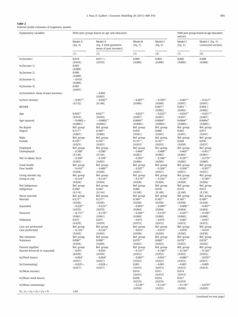
Table 2Ordered probit estimates of happiness models.

Explanatory variables With peer groups based on age and education With peer groups based on age educationand sex

Model A(Eq. 4)

Model A(Eq. 4 with geometricmean of past incomes)

Model B(Eq. 7)

Model C(Eq. 9)

Model C(Eq. 9)

Model C (Eq. 9)(restricted version)

(1) (2) (3) (4) (5) (6)

ln(Income) 0.014 0.017+ 0.009 0.004 0.006 0.008(0.010) (0.010) (0.006) (0.006) (0.006) (0.006)

ln(Income-1) 0.003(0.009)

ln(Income-2) 0.006(0.009)

ln(Income-3) −0.010(0.009)

ln(Income-4) 0.005(0.007)

ln(Geometric mean of past incomes) −0.002(0.005)

ln(Peer income) −0.967** −0.942** −0.407** −0.399** −0.407** −0.412**(0.152) (0.148) (0.049) (0.049) (0.047) (0.047)

RICHER 0.007** 0.003++ 0.004+(0.002) (0.002) (0.002)

Age 0.028** 0.027** −0.022** −0.022** −0.024** −0.021***(0.010) (0.010) (0.007) (0.007) (0.007) (0.007)

Age-squared −0.0002+ −0.0002** 0.0004** 0.0004** 0.0004** 0.0004**(0.0001) (0.0001) (0.0001) (0.0001) (0.0001) (0.0001)

No degree Ref. group Ref. group Ref. group Ref. group Ref. group Ref. groupDegree 0.317** 0.309** 0.054 0.060 0.062 0.071

(0.067) (0.066) (0.041) (0.041) (0.041) (0.041)Male Ref. group Ref. group Ref. group Ref. group Ref. group Ref. groupFemale 0.105** 0.105** 0.135** 0.143** 0.044 0.056

(0.025) (0.025) (0.033) (0.033) (0.038) (0.037)Employed Ref. group Ref. group Ref. group Ref. group Ref. group Ref. groupUnemployed −0.280* −0.280* −0.468** −0.488** −0.469** −0.451**

(0.136) (0.136) (0.081) (0.082) (0.082) (0.081)Not in labour force −0.200* −0.199* −0.285** −0.306** −0.287** −0.279**

(0.093) (0.093) (0.068) (0.069) (0.069) (0.069)Good health Ref. group Ref. group Ref. group Ref. group Ref. group Ref. groupPoor health −0.410** −0.409** −0.307** −0.306** −0.306** −0.307**

(0.028) (0.028) (0.021) (0.021) (0.021) (0.021)Living outside city Ref. group Ref. group Ref. group Ref. group Ref. group Ref. groupLiving in city −0.124** −0.124** −0.179** −0.182** −0.181** −0.189**

(0.024) (0.024) (0.028) (0.028) (0.028) (0.028)Not indigenous Ref. group Ref. group Ref. group Ref. group Ref. group Ref. groupIndigenous 0.280* 0.282* 0.084 0.078 0.074 0.072

(0.116) (0.116) (0.160) (0.160) (0.160) (0.159)Never married Ref. group Ref. group Ref. group Ref. group Ref. group Ref. groupMarried 0.272** 0.273** 0.384** 0.382** 0.385** 0.389**

(0.036) (0.036) (0.038) (0.038) (0.038) (0.038)Separated −0.226** −0.223** −0.405** −0.409** −0.408** −0.407**

(0.079) (0.079) (0.064) (0.064) (0.064) (0.064)Divorced −0.172** −0.170** −0.206** −0.210** −0.207** −0.198**

(0.061) (0.061) (0.060) (0.060) (0.060) (0.060)Widowed 0.073 0.075 −0.073 −0.079 −0.067 −0.057

(0.070) (0.070) (0.072) (0.072) (0.072) (0.072)Care not performed Ref. group Ref. group Ref. group Ref. group Ref. group Ref. groupCare performed −0.126** −0.126** −0.075* −0.075* −0.076* −0.076*

(0.043) (0.043) (0.030) (0.030) (0.030) (0.030)Not volunteer Ref. group Ref. group Ref. group Ref. group Ref. group Ref. groupVolunteer 0.098** 0.098** 0.079** 0.080** 0.078** 0.078**

(0.028) (0.028) (0.022) (0.022) (0.022) (0.022)Parents together Ref. group Ref. group Ref. group Ref. group Ref. group Ref. groupParents divorced or separated −0.051 −0.050 −0.141** −0.140** −0.144** −0.144**

(0.039) (0.039) (0.052) (0.052) (0.052) (0.052)ln(Work hours) −0.064* −0.064* −0.085** −0.092** −0.086** −0.076**

(0.027) (0.027) (0.022) (0.022) (0.022) (0.021)ln(Commuting) −0.029+ −0.028+ 0.001 −0.001 −0.001 −0.005

(0.017) (0.017) (0.015) (0.015) (0.015) (0.014)ln(Mean income) 0.014 0.011 0.014

(0.015) (0.015) (0.015)ln(Mean work hours) 0.028 0.024 0.027

(0.019) (0.019) (0.019)ln(Mean commuting) −0.120** −0.124** −0.118** −0.079**

(0.036) (0.035) (0.036) (0.029)Ho: β1=β2=β3=β4=0 1.64

(continued on next page)

905S. Paul, D. Guilbert / Economic Modelling 30 (2013) 900–910

12 See, for example, Blanchflower and Oswald (2004) for Britain and the US, andFerrer-i-Carbonell (2005) for Germany.13

Table 2 (continued)

Explanatory variables With peer groups based on age and education With peer groups based on age educationand sex

Model A(Eq. 4)

Model A(Eq. 4 with geometricmean of past incomes)

Model B(Eq. 7)

Model C(Eq. 9)

Model C(Eq. 9)

Model C (Eq. 9)(restricted version)

(1) (2) (3) (4) (5) (6)

χ2

Ho: β1+ β2 +β3+β4=0 0.43χ2

Wald-statistic 908.09** 905.69**Likelihood ratio 1238.78** 1249.23** 1246.89** 1244.02**χ2

No. of observations 8,530 8530 30,815 30,815 30,815 30,878

Note: Standard errors are reported in parentheses. In models A, standard errors are robust to heteroskedasticity. In all remaining models, results are derived using the REOPROBcommand in STATA 10.0. Unfortunately, there is currently no procedure that can be used to generate robust standard errors when using the REOPROB command. For this reason,the standard errors presented in models B and C are not robust to heteroskedasticity. **, *, + and ++ denote levels of significance respectively at the 1, 5, 10 and 15%.

906 S. Paul, D. Guilbert / Economic Modelling 30 (2013) 900–910

rejection of adaptation hypothesis might simply reflect the presence ofmeasurement errors in the income data. Peer group income, which iscalculated as the average income for a large group of people,11 is lesslikely to be subject to errors.

With no supporting evidence for adaptation, we drop all incomelags and proceed to estimate model B (Eq. 7) with the panel dataset for the period 2001–2005. This model incorporates individual ran-dom effects and makes use of the Mundlak correction to address thepossible correlation between unobservable personal traits and asub-set of explanatory variables. The results are presented in column3 of Table 2. Once again, current income has no statistically significanteffect upon life satisfaction. The coefficient on peer group income is−0.407 and this is statistically significant at the 1% level. This sug-gests that an increase in the average income level of the individual'speer group has a negative effect on the individual's life satisfaction.Since the coefficient of income (y) is 0.004 with a standard error of0.006, the negative and significant coefficient on peer group incomeimplies that a 1% rise in both personal income and peer group incomewould leave an individual worse off. A similar result is observed inClark and Oswald (1996) for Britain. In their study, the coefficient ofpeer group income is −0.2 with a standard error of 0.06 and that ofincome is 0.11 with a standard error of 0.050. The magnitude of thecomparison income effect in our study is stronger than that in Clarkand Oswald. We can think of two possible explanations for this.First, our method of computing comparison income (as discussed inSection 3) is different from that used in Clark and Oswald. The latterstudy estimates an earning equation to calculate comparison incomefor each individual. A comparison income is derived by predicting thetypical income of someone with the individual's observable charac-teristics. Second, the people in Australia could be more envious thanthose in Britain. The higher the degree of envy, the greater wouldbe the effect of peer group income on the individual's wellbeing. Ifthe degree of envy is zero, then peer group income would not affectthe wellbeing of an individual.

Finally, we turn to the estimation results based on model C (Eq. 9)which is designed to test the differential effects of peer group incomeon the wellbeing of poorer and richer individuals. The comparison in-come effect remains negative (−0.399) and statistically significant.The variable ‘RICHER’ has a positive coefficient (0.007) and is signifi-cant at the 1% level of confidence (Table 2, column 4). This suggeststhat an increase in peer group income affects the rich slightly lessthan it affects the poor. This is consistent with the results found inFerrer-i-Carbonell (2005) for Germany, and could imply that thereis a case for income redistribution, considering that greater incomeequality would raise the subjective wellbeing of the poor more thanit would reduce the subjective wellbeing of the rich. This study,

11 On average, there are about 860 individuals in each peer group constructed basedon age and education; some peer groups have over 2000 individuals.

however, finds no support for Runciman's theory of relative depriva-tion, which suggests that increases in peer group income do not hurtricher individuals.

The coefficients of control variables seem to be mostly in line withour expectations. Consistent with other studies, happiness is revealedto be U-shaped in age. However, unlike most studies, which find thathappiness minimises at around 40 years of age,12 this study finds thathappiness reaches a minimum during the late 20s. It appears that lifein Australia is most stressful for those in their late 20s, whosethoughts typically centre on concerns regarding social relationships,personal identity and uncertain career prospects. Females are signifi-cantly happier thanmales. While a similar result is reported in severalstudies including Clark and Oswald (1996) for Britain, Blanchflowerand Oswald (2004) for the US and Britain, and Headey and Wooden(2004) for Australia, no explanation is provided to explain this phe-nomenon. One possible reason is that women do more of pleasurableactivities such as leisure and looking after their children, whereasmales spend more time at work and less time with families andfriends. Another possible reason is that females might have verylow or no aspirations, whereas males have high aspirations which ifremain unfulfilled become the cause of their frustration. However,we do not have data on levels of aspirations of males and females toverify this point.

Suffering from poor health has a negative (−0.306) and signifi-cant effect upon life satisfaction. Marriage has a positive (0.385) andsignificant effect on life satisfaction, while separation and divorceexert negative and significant effect on life satisfaction. Married lifemore than neutralizes the consequences of poor health. Living in amajor city has a negative and significant effect upon life satisfaction.

Those who are unemployed or out of the labour force are less sat-isfied with life compared to those who are employed, although it isworth noting that the number of hours spent working each weekhas a negative impact upon life satisfaction. The finding that unem-ployment is a significant depressor of subjective wellbeing is consis-tent with the literature.13 Indeed, the effect of unemploymentappears to be stronger than the effect of divorce or separation i.e. iso-lation from one's spouse.

Those who perform volunteer or charity work tend to be happierthan those who do not. From a policy perspective this finding sug-gests that it could be worthwhile to put more effort into promotingvolunteer work and emphasising its benefits not only to the commu-nity but also to the volunteers themselves. Conversely, those who

See, for example, Clark and Oswald (1994) for Britain, Paul (1992) for the US,Blanchflower and Oswald (2004) for Britain and the US, Stutzer (2004) for Switzerland,and Dockery (2003), Paul (2001), Headey and Wooden (2004) and Carroll (2007) forAustralia.

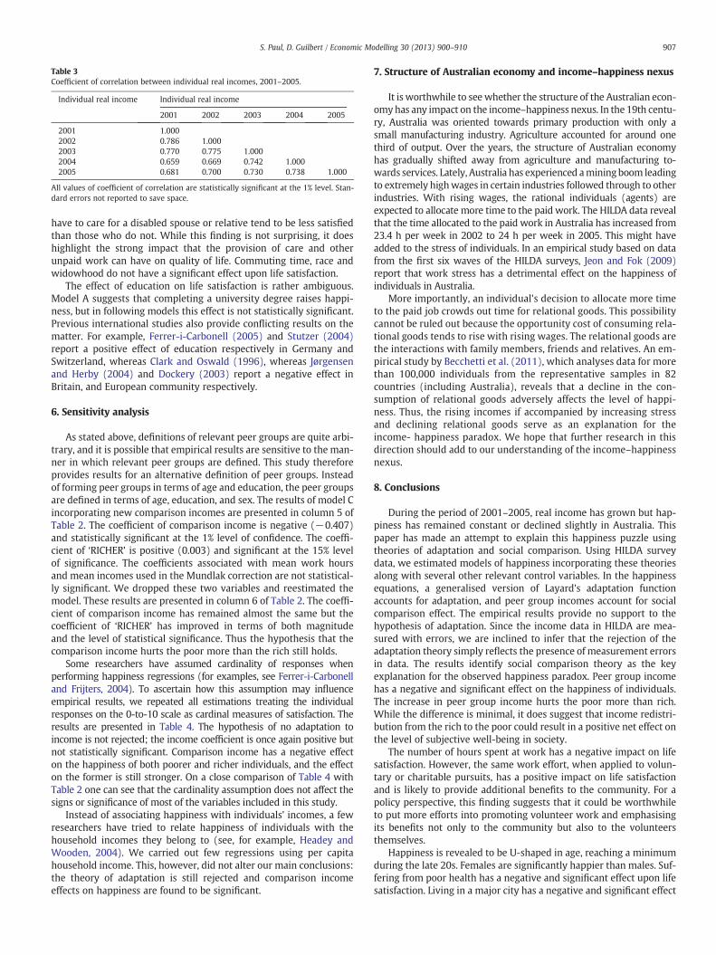
Table 3Coefficient of correlation between individual real incomes, 2001–2005.

Individual real income Individual real income

2001 2002 2003 2004 2005

2001 1.0002002 0.786 1.0002003 0.770 0.775 1.0002004 0.659 0.669 0.742 1.0002005 0.681 0.700 0.730 0.738 1.000

All values of coefficient of correlation are statistically significant at the 1% level. Stan-dard errors not reported to save space.

907S. Paul, D. Guilbert / Economic Modelling 30 (2013) 900–910

have to care for a disabled spouse or relative tend to be less satisfiedthan those who do not. While this finding is not surprising, it doeshighlight the strong impact that the provision of care and otherunpaid work can have on quality of life. Commuting time, race andwidowhood do not have a significant effect upon life satisfaction.

The effect of education on life satisfaction is rather ambiguous.Model A suggests that completing a university degree raises happi-ness, but in following models this effect is not statistically significant.Previous international studies also provide conflicting results on thematter. For example, Ferrer-i-Carbonell (2005) and Stutzer (2004)report a positive effect of education respectively in Germany andSwitzerland, whereas Clark and Oswald (1996), whereas Jørgensenand Herby (2004) and Dockery (2003) report a negative effect inBritain, and European community respectively.

6. Sensitivity analysis

As stated above, definitions of relevant peer groups are quite arbi-trary, and it is possible that empirical results are sensitive to the man-ner in which relevant peer groups are defined. This study thereforeprovides results for an alternative definition of peer groups. Insteadof forming peer groups in terms of age and education, the peer groupsare defined in terms of age, education, and sex. The results of model Cincorporating new comparison incomes are presented in column 5 ofTable 2. The coefficient of comparison income is negative (−0.407)and statistically significant at the 1% level of confidence. The coeffi-cient of ‘RICHER’ is positive (0.003) and significant at the 15% levelof significance. The coefficients associated with mean work hoursand mean incomes used in the Mundlak correction are not statistical-ly significant. We dropped these two variables and reestimated themodel. These results are presented in column 6 of Table 2. The coeffi-cient of comparison income has remained almost the same but thecoefficient of ‘RICHER’ has improved in terms of both magnitudeand the level of statistical significance. Thus the hypothesis that thecomparison income hurts the poor more than the rich still holds.

Some researchers have assumed cardinality of responses whenperforming happiness regressions (for examples, see Ferrer-i-Carbonelland Frijters, 2004). To ascertain how this assumption may influenceempirical results, we repeated all estimations treating the individualresponses on the 0-to-10 scale as cardinal measures of satisfaction. Theresults are presented in Table 4. The hypothesis of no adaptation toincome is not rejected; the income coefficient is once again positive butnot statistically significant. Comparison income has a negative effecton the happiness of both poorer and richer individuals, and the effecton the former is still stronger. On a close comparison of Table 4 withTable 2 one can see that the cardinality assumption does not affect thesigns or significance of most of the variables included in this study.

Instead of associating happiness with individuals’ incomes, a fewresearchers have tried to relate happiness of individuals with thehousehold incomes they belong to (see, for example, Headey andWooden, 2004). We carried out few regressions using per capitahousehold income. This, however, did not alter our main conclusions:the theory of adaptation is still rejected and comparison incomeeffects on happiness are found to be significant.

7. Structure of Australian economy and income–happiness nexus

It is worthwhile to see whether the structure of the Australian econ-omyhas any impact on the income–happiness nexus. In the 19th centu-ry, Australia was oriented towards primary production with only asmall manufacturing industry. Agriculture accounted for around onethird of output. Over the years, the structure of Australian economyhas gradually shifted away from agriculture and manufacturing to-wards services. Lately, Australia has experienced aminingboom leadingto extremely highwages in certain industries followed through to otherindustries. With rising wages, the rational individuals (agents) areexpected to allocate more time to the paid work. The HILDA data revealthat the time allocated to the paid work in Australia has increased from23.4 h per week in 2002 to 24 h per week in 2005. This might haveadded to the stress of individuals. In an empirical study based on datafrom the first six waves of the HILDA surveys, Jeon and Fok (2009)report that work stress has a detrimental effect on the happiness ofindividuals in Australia.

More importantly, an individual's decision to allocate more timeto the paid job crowds out time for relational goods. This possibilitycannot be ruled out because the opportunity cost of consuming rela-tional goods tends to rise with rising wages. The relational goods arethe interactions with family members, friends and relatives. An em-pirical study by Becchetti et al. (2011), which analyses data for morethan 100,000 individuals from the representative samples in 82countries (including Australia), reveals that a decline in the con-sumption of relational goods adversely affects the level of happi-ness. Thus, the rising incomes if accompanied by increasing stressand declining relational goods serve as an explanation for theincome- happiness paradox. We hope that further research in thisdirection should add to our understanding of the income–happinessnexus.

8. Conclusions

During the period of 2001–2005, real income has grown but hap-piness has remained constant or declined slightly in Australia. Thispaper has made an attempt to explain this happiness puzzle usingtheories of adaptation and social comparison. Using HILDA surveydata, we estimated models of happiness incorporating these theoriesalong with several other relevant control variables. In the happinessequations, a generalised version of Layard's adaptation functionaccounts for adaptation, and peer group incomes account for socialcomparison effect. The empirical results provide no support to thehypothesis of adaptation. Since the income data in HILDA are mea-sured with errors, we are inclined to infer that the rejection of theadaptation theory simply reflects the presence of measurement errorsin data. The results identify social comparison theory as the keyexplanation for the observed happiness paradox. Peer group incomehas a negative and significant effect on the happiness of individuals.The increase in peer group income hurts the poor more than rich.While the difference is minimal, it does suggest that income redistri-bution from the rich to the poor could result in a positive net effect onthe level of subjective well-being in society.

The number of hours spent at work has a negative impact on lifesatisfaction. However, the same work effort, when applied to volun-tary or charitable pursuits, has a positive impact on life satisfactionand is likely to provide additional benefits to the community. For apolicy perspective, this finding suggests that it could be worthwhileto put more efforts into promoting volunteer work and emphasisingits benefits not only to the community but also to the volunteersthemselves.

Happiness is revealed to be U-shaped in age, reaching a minimumduring the late 20s. Females are significantly happier than males. Suf-fering from poor health has a negative and significant effect upon lifesatisfaction. Living in a major city has a negative and significant effect

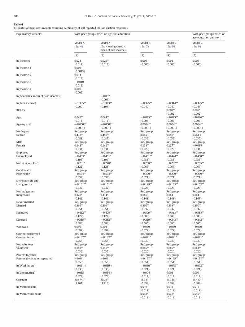
Table 4Estimates of happiness models assuming cardinality of self reported life satisfaction responses.

Explanatory variables With peer groups based on age and education With peer groups based onage education and sex

Model A(Eq. 4)

Model A(Eq. 4 with geometricmean of past incomes)

Model B(Eq. 7)

Model C(Eq. 9)

Model C(Eq. 9)

(1) (2) (3) (4) (5)

ln(Income) 0.021 0.026** 0.009 0.003 0.005(0.014) (0.013) (0.006) (0.006) (0.006)

ln(Income-1) 0.002(0.0013)

ln(Income-2) 0.011(0.013)

ln(Income-3) −0.010(0.012)

ln(Income-4) 0.007(0.009)

ln(Geometric mean of past incomes) −0.002(0.007)

ln(Peer income) −1.385** −1.343** −0.325** −0.314** −0.325**(0.200) (0.194) (0.049) (0.049) (0.046)

RICHER 0.008** 0.005*(0.002) (0.002)

Age 0.042** 0.041** −0.025** −0.025** −0.026**(0.013) (0.013) (0.007) (0.007) (0.007)

Age-squared −0.0003* −0.0003* 0.0004** 0.0004** 0.0004**(0.0001) (0.0001) (0.0001) (0.0001) (0.0001)

No degree Ref. group Ref. group Ref. group Ref. group Ref. groupDegree 0.472** 0.459** 0.055 0.059* 0.064+

(0.088) (0.087) (0.036) (0.036) (0.035)Male Ref. group Ref. group Ref. group Ref. group Ref. groupFemale 0.148** 0.146** 0.128** 0.137** −0.018

(0.034) (0.034) (0.029) (0.029) (0.034)Employed Ref. group Ref. group Ref. group Ref. group Ref. groupUnemployed −0.453* −0.451* −0.451** −0.474** −0.458**

(0.196) (0.196) (0.085) (0.085) (0.085)Not in labour force −0.251* −0.248* −0.258** −0.282** −0.265**

(0.122) (0.123) (0.066) (0.067) (0.067)Good health Ref. group Ref. group Ref. group Ref. group Ref. groupPoor health −0.574** −0.573** −0.300** −0.299** −0.299**

(0.039) (0.039) (0.021) (0.021) (0.021)Living outside city Ref. group Ref. group Ref. group Ref. group Ref. groupLiving in city −0.151** −0.151** −0.149** −0.153** −0.152**

(0.032) (0.032) (0.026) (0.026) (0.026)Not indigenous Ref. group Ref. group Ref. group Ref. group Ref. groupIndigenous 0.328* 0.331* 0.086 0.081 0.081

(0.149) (0.149) (0.148) (0.148) (0.147)Never married Ref. group Ref. group Ref. group Ref. group Ref. groupMarried 0.364** 0.366** 0.360** 0.358** 0.360**

(0.051) (0.051) (0.037) (0.037) (0.037)Separated −0.412** −0.408** −0.509** −0.513** −0.513**

(0.122) (0.122) (0.080) (0.080) (0.080)Divorced −0.285** −0.282** −0.239** −0.243** −0.242**

(0.089) (0.089) (0.065) (0.065) (0.065)Widowed 0.099 0.103 −0.060 −0.069 −0.059

(0.092) (0.092) (0.077) (0.077) (0.077)Care not performed Ref. group Ref. group Ref. group Ref. group Ref. groupCare performed −0.167** −0.167** −0.071* −0.071* −0.071*

(0.058) (0.058) (0.030) (0.030) (0.030)Not volunteer Ref. group Ref. group Ref. group Ref. group Ref. groupVolunteer 0.158** 0.157** 0.085** 0.085** 0.084**

(0.036) (0.035) (0.020) (0.020) (0.020)Parents together Ref. group Ref. group Ref. group Ref. group Ref. groupParents divorced or separated −0.071 −0.071 −0.157** −0.155** −0.157**

(0.055) (0.055) (0.051) (0.051) (0.051)ln(Work hours) −0.061+ −0.059+ −0.069** −0.078** −0.072**

(0.036) (0.036) (0.021) (0.021) (0.021)ln(Commuting) −0.035 −0.034+ −0.004 0.003 0.004

(0.022) (0.022) (0.014) (0.014) (0.014)Constant 20.574** 20.22** 11.351** 11.336** 11.487**

(1.761) (1.713) (0.398) (0.398) (0.389)ln(Mean income) 0.016 0.012 0.014

(0.014) (0.014) (0.014)ln(Mean work hours) 0.042* 0.037* 0.040*

(0.018) (0.018) (0.018)

908 S. Paul, D. Guilbert / Economic Modelling 30 (2013) 900–910

Table 4 (continued)

Explanatory variables With peer groups based on age and education With peer groups based onage education and sex

Model A(Eq. 4)

Model A(Eq. 4 with geometricmean of past incomes)

Model B(Eq. 7)

Model C(Eq. 9)

Model C(Eq. 9)

(1) (2) (3) (4) (5)

ln(Mean commuting) −0.099** −0.103** −0.099**(0.030) (0.030) (0.030)

Ho: β1=β2=…=βk=0 0.45F-value (4, 8505)R-squared 0.10 0.10Wald statistic 1075.52** 1088.97** 1088.20**No. of observations 8530 8530 30,815 30,815 30,815

Note: Model A is estimated by OLS and models B and C are estimated by GLS with random effects. Standard errors are reported in parentheses and are robust to heteroskedasticity.**, *, and + denote levels of significance respectively at the 1, 5 and 10%.

909S. Paul, D. Guilbert / Economic Modelling 30 (2013) 900–910

upon life satisfaction. Being married contributes to happiness, whilebecoming separated or divorced causes a reduction in life satisfaction.Those who are unemployed or out of the labour force are less satisfiedwith life compared to those who are employed. Those who have tocare for a disabled spouse or relative tend to be less satisfied thanthose who do not.

Finally, it is worth noting that the phenomenon of economicgrowth with flat or declining happiness does not necessarily mean

Table AOrdered probit estimates of happiness model A (Eq. 4) with alternative lags of income and

Variables Model A (Eq. 4) (without ‘RICHER’ variable)

(1) (2) (3)

ln(Income) 0.028** 0.012 0.009(0.008) (0.007) (0.006)

ln(Income-1) 0.010 0.019* 0.011*(0.009) (0.007) (0.005)

ln(Income-2) 0.007 0.002(0.008) (0.006)

ln(Income-3) −0.001(0.008)

ln(Income-4)

All other variables included in estimation. Results not presented to save spaceWald statisticsLikelihood ratioχ2 1162.9** 1363.0** 1501.0**No. of observations 16030 23746 31562

Note: **, * and + denote respectively significant at the 1, 5 and 10%.

that economic growth should not be the goal of economic policy.After all, economic growth is likely to increases the tax yield whichis often used to fund public services that may themselves enhancewellbeing in society. However, our results reveal that there issome merit in policymakers giving more attention to the pursuits ofother objectives (e.g. promoting health and reducing unemploy-ment) which are likely to provide greater benefits in terms of lifesatisfaction.

Appendix A

with and without ‘RICHER’ variable.

Model A (Eq. 4) (with ‘RICHER’ variable)

(4) (5) (6) (7)

0.005 0.020 0.005 0.003(0.010) (0.009) (0.007) (0.006)0.001 0.008 0.017* 0.009+(0.009) (0.008) (0.007) (0.005)0.004 0.005 0.001(0.009) (0.008) (0.006)−0.011 −0.007(0.009) (0.007)0.004(0.007)

920.91**

1171.4** 1373.6** 1514.7**8530 16030 23746 51562

References

Australian Bureau of Statistics, 2007. Consumer Price Index, Australia. Catalogue No. 6401.0.Becchetti, L., Trovato, G., Bedoya, D.A., 2011. Income, relational goods and happiness.

Applied Economics 43, 273–290.Blanchflower, D.G., Oswald, A.J., 2004. Well-being over time in Britain and the USA.

Journal of Public Economics 88 (7–8), 1359–1386.Bossert, W., Ambrosio, C., 2007. Dynamic measures of individual deprivation. Social

Choice and Welfare 28, 77–88.Brickman, P., Coates, D., Janoff-Bulman, R., 1978. Lottery winners and accident victims: is

happiness relative? Journal of Personality and Social Psychology 36 (8), 917–927.Carroll, N., 2007. Unemployment and psychological well-being. The Economic Record 83

(262), 287–302.

Clark, A.E., Oswald, A.J., 1994. Happiness and unemployment. The Economic Journal 104(424), 648–659.

Clark, A.E., Oswald, A.J., 1996. Satisfaction and comparison income. Journal of PublicEconomics 61 (3), 359–381.

Clark, A.E., Frijters, P., Shields, M., 2008. Relative income, happiness and utility: anexplanation for the Easterlin paradox and other puzzles. Journal of EconomicLiterature 46 (1), 95–144.

Di Tella, R., MacCulloch, R., Oswald, A.J., 2003. The macroeconomics of happiness. TheReview of Economics and Statistics 85 (1), 809–827.

Di Tella, R., Haiskens-De New, J., MacCulloch, R., 2007. Happiness adaptation toincome and to status in an individual panel. (NBER Working Paper # W13159,June).

Dockery, A.M., 2003. Happiness, life satisfaction and the role of work: evidence from twoAustralian surveys. Curtin University of Technology . (Working paper # 03/10).

910 S. Paul, D. Guilbert / Economic Modelling 30 (2013) 900–910

Duesenberry, J.S., 1949. Income, saving and the theory of consumer behaviour. HarvardUniversity Press, Cambridge, MA.

Easterlin, R., 1974. Does economic growth improve the human lot? In: David, Paul A.,Reder, Melvin W. (Eds.), Nations and households in economic growth: essays inthe honor of Moses Abramovitz. Academic Press, New York.

Easterlin, R., 1995. Will raising the incomes of all increase the happiness of all? Journalof Economic Behavior and Organization 27 (1), 35–47.

Easterlin, R., Angelescu, L., 2009. Happiness and growth the world over: time seriesevidence on the happiness-income paradox . (IZA Discussion Paper # 460, March).

Ferrer-i-Carbonell, A., 2005. Income and well-being: an empirical analysis of the com-parison income effect. Journal of Public Economics 89 (5–6), 997–1019.

Ferrer-i-Carbonell, A., Frijters, P., 2004. How important ismethodology for the estimates ofthe determinants of happiness? The Economic Journal 114 (497), 641–659.

Gilbert, D., 2006. Stumbling on happiness. Harper Press, London.Headey, B., Wooden, M., 2004. The effects of wealth and income on subjective

well-being and ill-being. Economic Record 80, September, Special Issue,pp. S24–S33.

Hsiao, C., 1986. Analysis of panel data. Cambridge University Press, New York.Inglehart, R., Klingemann, H.D., 2000. Genes, culture, democracy, and happiness.

In: Diener, E., Suh, E.M. (Eds.), Culture and subjective well-being. MIT Press,Cambridge.

Jeon, S., Fok, Y.K., 2009. Work and mental well-being: work stress and mental well-being of the Australian working population. (Project # 5/08) Melbourne Instituteof Applied Economic and Social Research. (June).

Jørgensen, C.B., Herby, J., 2004. Do people care about relative income? Centre for Economicand Business Research, University of Copenhagen. (Student Paper 2004-01).

Layard, R., 2005. Happiness: lessons from a new science. Penguin Books, London.Luttmer, E., 2005. Neighbours as negatives: relative earnings and wellbeing. Quarterly

Journal of Economics 120 (3), 963–1002.McBride, M., 2001. Relative-income effects on subjective well-being in the cross-section.

Journal of Economic Behavior and Organization 45 (3), 251–278.

Miles, D., Rossi, M., 2007. Learning about one's relative position and subjectivewell-being.Applied Economics 39 (13), 1711–1718.

Mundlak, Y., 1978. On the pooling of time series and cross section data. Econometrica46 (1), 69–85.

Neumark, D., Postlewaite, A., 1998. Relative income concerns and the rise in marriedwomen's employment. Journal of Public Economics 70 (1), 157–183.

Paul, S., 1991. An index of relative deprivation. Economics Letters 36, 567–573.Paul, S., 1992. An illfare approach to the measurement of unemployment. Applied

Economics 24, 737–743.Paul, S., 2001. A welfare loss measure of unemployment with an empirical illustration.

The Manchester School 69 (2), 148–163.Runciman, W., 1966. Relative deprivation and social justice. Routledge and Kegan Paul,

London.Schimmack, U., 2006. Internal and external determinants of subjective well-being:

review and policy implications. In: Ng, Y.K., Ho, L.S. (Eds.), Happiness and publicpolicy: theory, case studies and implications. Palgrave Macmillan, New York.

Senik, C., 2004. When information dominates comparison: learning from Russiansubjective panel data”. Journal of Public Economics 88 (8–9), 2099–2123.

Solnick, S.J., Hemenway, D., 1998. Is more always better? A survey on positionalconcerns. Journal of Economic Behavior and Organization 37 (3), 373–383.

Stutzer, A., 2004. The role of income aspirations in individual happiness. Journal ofEconomic Behavior and Organization 54 (1), 89–109.

Stutzer, A., Frey, Buno S., 2004. Reported subjective well-being: a challenge for economictheory and economic policy. Schmollers Jahrbuch 124 (2), 191–231.

van de Stadt, H., Kapteyn, A., van de Geer, S., 1985. The relativity of utility: evidencefrom panel data. The Review of Economics and Statistics 67 (2), 179–187.

Wilkins, R., 2009. Updates and revisions to estimates of income tax and governmentbenefits. (Hilda Project Discussion Paper Series # 1/09, February)Melbourne Instituteof Applied Economic and Social Research, Melbourne University.

Yitzhaki, S., 1979. Relative deprivation and the Gini coefficient. Quarterly Journal ofEconomics 93, 321–324.