Embed Size (px)
Citation preview
INCOMPRESSIBLE VISCOUS IN A DRIVEN CAVITY
A N COPY: R W BFWL TECHNICAL I
NATIONAL AERONAUTICS AND SPACE ADMINISTRAT
https://ntrs.nasa.gov/search.jsp?R=19760008935 2019-01-21T23:14:56+00:00Z
NASA SP-378
TECH LIBRARY KAFB, NM
NUMERICAL STUDIES OFINCOMPRESSIBLE VISCOUS FLOW
A DRIVEN CAVITY
By the Staff of Langley Research Center
Scientific and Technical Information Office 1975NATIONAL AERONAUTICS AND SPACE ADMINISTRATION
Washington, D.C.
For sale by the National Technical Information ServiceSpringfield, Virginia 22161Price - $5.75
PREFACE
This publication consists of a series of project papers prepared by graduate stu-dents in computational fluid dynamics. The work was performed during the 1973-74academic year at Old Dominion University under the auspices of Professor Stanley G.Rubin, now with the Polytechnic Institute of New York. The class, taught at LangleyResearch Center, was comprised of Langley employees and contractors. Each paperbriefly examines one of the numerical methods discussed during the lectures andapplies the method to the Navier-Stokes equations governing incompressible flow in adriven cavity. Also, solutions obtained with a cubic spline procedure which was underinvestigation at the time are included.
It should be emphasized that most of these studies were completed in a period ofapproximately 6 weeks by different researchers with backgrounds varying from fluidmechanics to applied mathematics. (All had considerable experience with numericalcomputations.) Therefore, this publication should not be used as a definitive comparisonof the various numerical methods discussed, since this would require a more extensiveand unified study.
The results and discussion presented are instructive in that:
(1) They demonstrate a number of numerical procedures applied by experiencednumerical analysts who, however, were not expert in the use of these methods and wererequired to complete their analyses within a specified time period.
(2) They include solutions for both primitive-variable and vorticity—stream-function systems of equations.
(3) They present solutions for the driven cavity obtained with popular numericalprocedures (such as alternating direction implicit, successive overrelaxation, and Mar-ker and Cell) as well as with several techniques that have not been applied extensively(e.g., direct Poisson solvers, spline methods, weighted differencing, artificial compres-sibility, and hopscotch).
(4) They include some solutions for Reynolds numbers larger than those for whichsolutions have previously been reported in the literature. This publication is consideredsuitable for providing graduate students and practitioners of computational fluid dynam-ics with reference material covering a relatively broad spectrum of numerical proce-dures for solving the Navier-Stokes equations.

Page Intentionally Left Blank
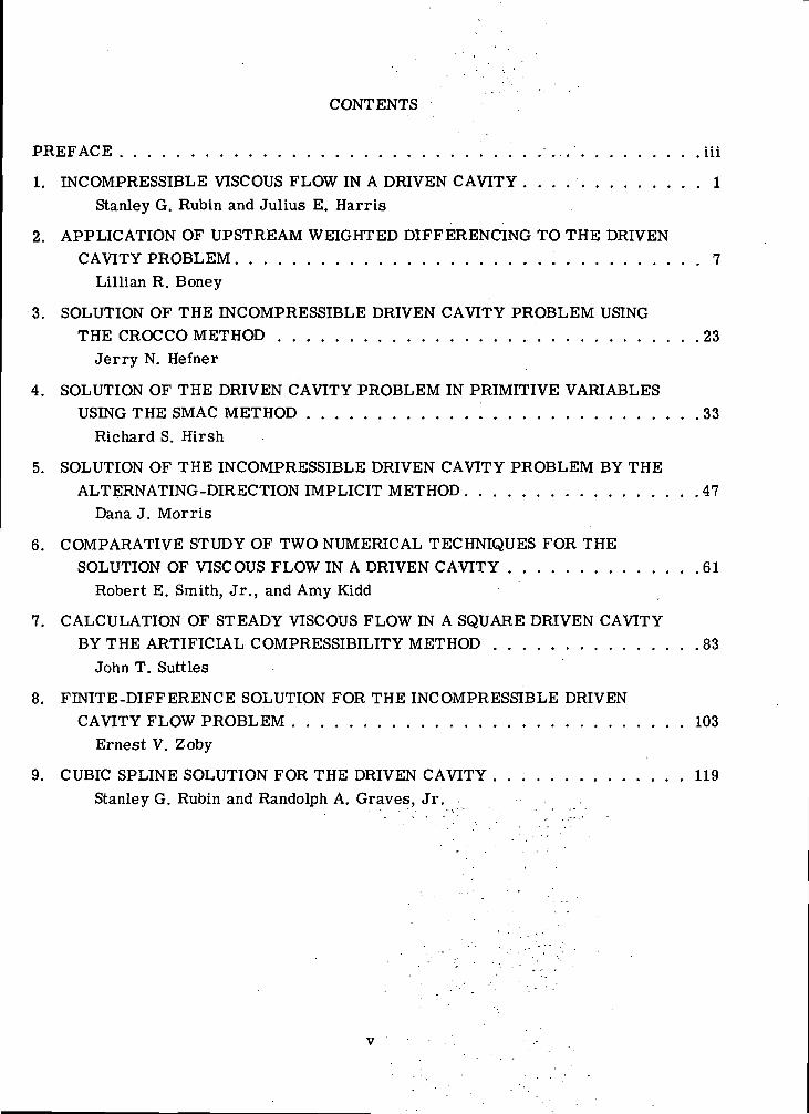
CONTENTS
PREFACE iii
1. INCOMPRESSIBLE VISCOUS FLOW IN A DRIVEN CAVITY . . . 1
Stanley G. Rubin and Julius E. Harris
2. APPLICATION OF UPSTREAM WEIGHTED DIFFERENCING TO THE DRIVENCAVITY PROBLEM 7
Lillian R. Boney
3. SOLUTION OF THE INCOMPRESSIBLE DRIVEN CAVITY PROBLEM USINGTHE CROCCO METHOD 23
Jerry N. Hefner
4. SOLUTION OF THE DRIVEN CAVITY PROBLEM IN PRIMITIVE VARIABLESUSING THE SMAC METHOD 33
Richard S. Hirsh
5. SOLUTION OF THE INCOMPRESSIBLE DRIVEN CAVITY PROBLEM BY THEALTERNATING-DIRECTION IMPLICIT METHOD 47
Dana J. Morris
6. COMPARATIVE STUDY OF TWO NUMERICAL TECHNIQUES FOR THESOLUTION OF VISCOUS FLOW IN A DRIVEN CAVITY 61
Robert E. Smith, Jr., and Amy Kidd
7. CALCULATION OF STEADY VISCOUS FLOW IN A SQUARE DRIVEN CAVITYBY THE ARTIFICIAL COMPRESSIBILITY METHOD 83
John T. Suttles
8. FINITE-DIFFERENCE SOLUTION FOR THE INCOMPRESSIBLE DRIVENCAVITY FLOW PROBLEM 103
Ernest V. Zoby
9. CUBIC SPLINE SOLUTION FOR THE DRIVEN CAVITY 119Stanley G. Rubin and Randolph A. Graves, Jr. .
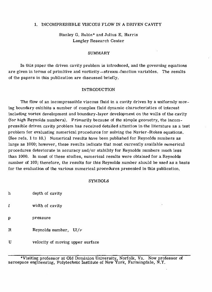
1. INCOMPRESSIBLE VISCOUS FLOW IN A DRIVEN CAVITY
Stanley G. Rubin* and Julius E. HarrisLangley Research Center
SUMMARY
In this paper the driven cavity problem is introduced, and the governing equationsare given in terms of primitive and vorticity—stream-function variables. The resultsof the papers in this publication are discussed briefly.
INTRODUCTION
The flow of an incompressible viscous fluid in a cavity driven by a uniformly mov-ing boundary exhibits a number of complex fluid dynamic characteristics of interestincluding vortex development and boundary-layer development on the walls of the cavity(for high Reynolds numbers). Primarily because of the simple geometry, the incom-pressible driven cavity problem has received detailed attention in the literature as a testproblem for evaluating numerical procedures for solving the Navier-Stokes equations.(See refs. 1 to 10.) Numerical results have been published for Reynolds numbers aslarge as 1000; however, these results indicate that most currently available numericalprocedures deteriorate in accuracy and/or stability for Reynolds numbers much lessthan 1000. In most of these studies, numerical results were obtained for a Reynoldsnumber of 100; therefore, the results for this Reynolds number should be used as a basisfor the evaluation of the various numerical procedures presented in this publication.
SYMBOLS
h depth of cavity
I width of cavity
p pressure
R Reynolds number, UZ/f
U velocity of moving upper surface
*Visiting professor at Old Dominion University, Norfolk, Va. Now professor ofaerospace engineering, Polytechnic Institute of New York, Farmingdale, N.Y.
u,v velocity component in x-and y-direction, respectively
x,y rectangular coordinates defined in figure 1
£ vorticity
v kinematic viscosity
p density
4* stream function
Subscripts:
t differentiation with respect to time
x,y differentiation with respect to x or y
STATEMENT OF PROBLEM
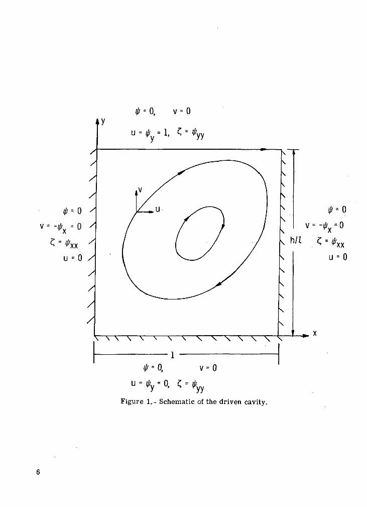
In the present publication, incompressible viscous flow in a cavity driven by a uni-formly moving upper surface (see fig. 1) is predicted by several numerical techniques.Solutions are obtained for the Navier-Stokes and continuity equations written in eitherprimitive or vorticity—stream-function variables. These equations are as follows:
Primitive variables
Continuity
ux + vy = 0 (la)
x-momentum
Ut + UUX + VUy = -Px + R-^Uxx + Uyy)
y-momentum
Vt + UVX + Wy = -Py + R-^Vxx + Vyy)
Vorticity—stream-function variables
Vorticity
? t + u? x + v?y = R-1(?xx+?yy) (2a)
Stream function
^xx+ *yy = ? . (2b)
All quantities are nondimensional. Velocities have been nondimensionalized with U,lengths with I, pressure with pU , and time with l/\J.
The boundary conditions are presented in figure 1. In several papers containedherein the authors consider a plate moving from right to left so that u = i//y = -1 at theupper boundary; in addition, £ is defined as vx - uy. Direct comparisons with solu-tions for a plate moving with u = 1 are possible if u, v, and ^/ are replaced with-u, -v, and -i//, respectively.
DISCUSSION OF RESULTS
In each paper included in the present publication the square driven cavity has beenstudied for a standard test case of R = 100. This particular case has received the mostdetailed attention in the literature. In addition to the standard test case, numericalresults are presented in some papers for values of R of 10, 1000, and 5000. Somesolutions are also given for rectangular cavities having width-depth ratios of 2 and 4.Solutions for R = 5000 were obtained with a central-difference alternating-directionimplicit procedure for the vorticity equation and a successive over relaxation or a directPoisson solver for the stream function. These results for the driven cavity represent,to the best of the authors' knowledge, solutions for the highest Reynolds number currentlyavailable in the literature. Other results were obtained with hopscotch, Marker-and -Cell, spline integration, Crocco, weighted-differencing, Chorin, and Spalding procedures.
The results presented in the papers indicate that convergence was more rapid withthe vorticity—stream-function formulation. The accuracy of the primitive-variable solu-tions was extremely sensitive to the convergence tolerance assigned to the pressure sol-ver. As this criterion was refined, computational times escalated.
Divergence form calculations were more accurate than nondivergence results,except for the nondivergence spline solutions. These were more accurate than any of thefinite-difference results. This would reflect the higher order accuracy of the convectionterms in the spline procedure.
3
It should be carefully noted that the computer codes developed for the procedureswere not necessarily optimized; consequently, no comparisons among the papers arepresented concerning computational efficiency (computer processing time and storagerequirements). However, the numerical procedures are developed in sufficient detail sothat they could be easily used by those interested in either making direct comparisons orapplying the procedures to other problems. The intent of the authors is that the presentpublication should be an outline of the development of specific numerical procedures andtheir application to a standard test problem. From this viewpoint, the potential users ofthe various numerical techniques should be able to select the specific procedure whichwould best satisfy their particular computational requirements.
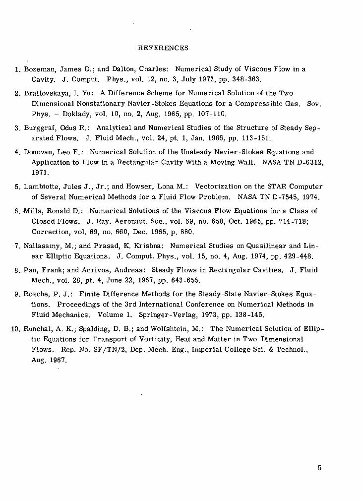
REFERENCES
1. Bozeman, James D.; and Dalton, Charles: Numerical Study of Viscous Flow in aCavity. J. Comput. Phys., vol. 12, no. 3, July 1973, pp. 348-363.
2. Brailovskaya, I. Yu: A Difference Scheme for Numerical Solution of the Two-Dimensional Nonstationary Navier-Stokes Equations for a Compressible Gas. Sov.Phys. - Doklady, vol. 10, no. 2, Aug. 1965, pp. 107-110.
3. Burggraf, Odus R.: Analytical and Numerical Studies of the Structure of Steady Sep-arated Flows. J. Fluid Mech., vol. 24, pt. 1, Jan. 1966, pp. 113-151.
4. Donovan, Leo F.: Numerical Solution of the Unsteady Navier-Stokes Equations andApplication to Flow in a Rectangular Cavity With a Moving Wall. NASA TN D-6312,1971.
5. Lambiotte, Jules J., Jr.; and Howser, Lona M.: Vectorization on the STAR Computerof Several Numerical Methods for a Fluid Flow Problem. NASA TN D-7545, 1974.
6. Mills, Ronald D.: Numerical Solutions of the Viscous Flow Equations for a Class ofClosed Flows. J. Ray. Aeronaut. Soc., vol. 69, no. 658, Oct. 1965, pp. 714-718;Correction, vol. 69, no. 660, Dec. 1965, p. 880.
7. Nallasamy, M.; and Prasad, K. Krishna: Numerical Studies on Quasilinear and Lin-ear Elliptic Equations. J. Comput. Phys., vol. 15, no. 4, Aug. 1974, pp. 429-448.
8. Pan, Frank; and Acrivos, Andreas: Steady Flows in Rectangular Cavities. J. FluidMech., vol. 28, pt. 4, June 22, 1967, pp. 643-655.
9. Roache, P. J.: Finite Difference Methods for the Steady-State Navier-Stokes Equa-tions. Proceedings of the 3rd International Conference on Numerical Methods inFluid Mechanics. Volume 1. Springer-Verlag, 1973, pp. 138-145.
10. Runchal, A. K.; Spalding, D. B.; and Wolfshtein, M.: The Numerical Solution of Ellip-tic Equations for Transport of Vorticity, Heat and Matter in Two-DimensionalFlows. Rep. No. SF/TN/2, Dep. Mech. Eng., Imperial College Sci. & Technol.,Aug. 1967.
X
= 0, v = 0
U - ,
/
0 = 0
v = -0X = 0
u = 0 X
s, h/l
u = 0
\ \ \ \ \ N \ \ N N \ \ \ \ \
= 0, v = 0
Figure 1.- Schematic of the driven cavity.
2. APPLICATION OF UPSTREAM WEIGHTED DIFFERENCING
TO THE DRIVEN CAVITY PROBLEM
Lillian R. BoneyLangley Research Center
SUMMARY
The problem considered is steady plane flow of an incompressible viscous fluid ina two-dimensional square cavity in which the motion is driven by uniform translation ofthe upper wall which moves across the cavity from left to right at a constant speed of 1.Numerical solutions of the Navier-Stokes equations are obtained for a range of Reynoldsnumber from 100 to 1000. Upstream weighted differencing is used when the local cellReynolds number exceeds 2.
INTRODUCTION
It is well-known that the flow of viscous fluid can be treated successfully with theNavier-Stokes equations. Many authors have examined finite-difference solutions of theequations of steady-state motion and continuity in a two-dimensional domain. Somefound that unless the mesh size was severely reduced, their computational proceduresfailed to converge when the Reynolds number became large.
This paper treats steady plane flow of an incompressible viscous fluid in a two-dimensional square cavity in which the motion is driven by uniform translation of theupper wall which moves across the cavity from left to right at a constant speed of 1.(See paper no. 1 by Rubin and Harris.) The two momentum equations and the continuityequation, written in normalized conservative form in terms of the primitive variables(velocity components u and v and the pressure p), are used rather than the stream -function and vorticity transport equations. The pressure term is treated by a Poissonequation. The primitive-variable system involves two parabolic momentum transportequations and one elliptic equation with all Neumann boundaries. Upstream weighteddifferencing (ref. 1) for the velocity gradients is chosen for its good stability propertiesand the transportive property which finite-difference formulation of a flow equation pos-sesses if the effect of a perturbation in a transport property is advected only in thedirection of the velocity.
• 7
SYMBOLS
K constant in equation (5)
p pressure
p error in initial estimate of p
p initial estimate of p
R Reynolds number
Rc cell Reynolds number
S = v2p
t time
At time step
u axial velocity component
v normal velocity component
W * weighting factor based on Rc (see eqs. (7))
w factor in equation (22)
x axial coordinate
y normal coordinate
Ax, Ay grid spacing in x- and y-directions
/3 = Ax/Ay
Superscripts:
k index of iteration
n index of time step
Subscripts:
i,j index of grid spacing in x- and y-direction, respectively
ref reference
GOVERNING EQUATIONS
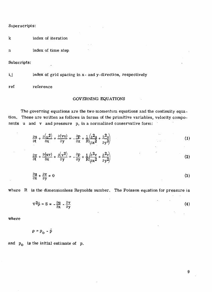
The governing equations are the two momentum equations and the continuity equation. These are written as follows in forms of the primitive variables, velocity components u and v and pressure p, in a normalized conservative form:
8u i a(u2) . 8(vu) _ 3P . 1 /32u . 92u\ " /at 9x + ay ~ ax + R^X2 +
ay2J
9v . 9(uv) . a(v2) _ £P 1 /32V 92v\ ' (at ax + ay ' ay + R^X2 +
9y2/
where R is the dimensionless Reynolds number. The Poisson equation for pressure is
V2p.S= . |H.g (4,
where
P = P0 - P
and p0 is the initial estimate of p.
FINITE-DIFFERENCE REPRESENTATIONS
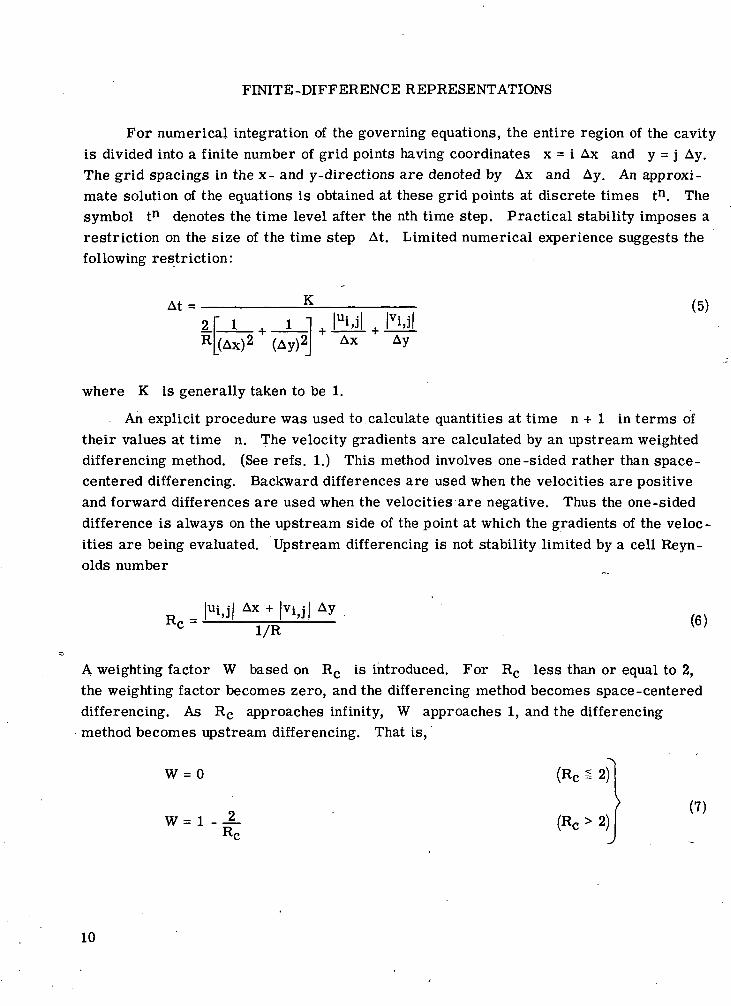
For numerical integration of the governing equations, the entire region of the cavityis divided into a finite number of grid points having coordinates x = i Ax and y = j Ay.The grid spacings in the x- and y-directions are denoted by Ax and Ay. An approxi-mate solution of the equations is obtained at these grid points at discrete times tn. Thesymbol tn denotes the time level after the nth time step. Practical stability imposes arestriction on the size of the time step At. Limited numerical experience suggests thefollowing restriction:
At = K_ . . (5)K
2f ! .Rl(Ax)21 1 , |ui,i , vul
(Ay)2| Ax AY
where K is generally taken to be 1.
An explicit procedure was used to calculate quantities at time n + 1 in terms oftheir values at time n. The velocity gradients are calculated by an upstream weighteddifferencing method. (See refs. 1.) This method involves one-sided rather than space-centered differencing. Backward differences are used when the velocities are positiveand forward differences are used when the velocities are negative. Thus the one-sideddifference is always on the upstream side of the point at which the gradients of the veloc-ities are being evaluated. Upstream differencing is not stability limited by a cell Reyn-olds number
_ |uj,j| Ax + |vy[ AyK C ~ V R " ( 6 )
A weighting factor W based on Rc is introduced. For Rc less than or equal to 2,the weighting factor becomes zero, and the differencing method becomes space-centereddifferencing. As Rc approaches infinity, W approaches 1, and the differencingmethod becomes upstream differencing. That is,
W = 0 (Rc = 2)!
W = 1 - J T ( R c>2)Kc
10
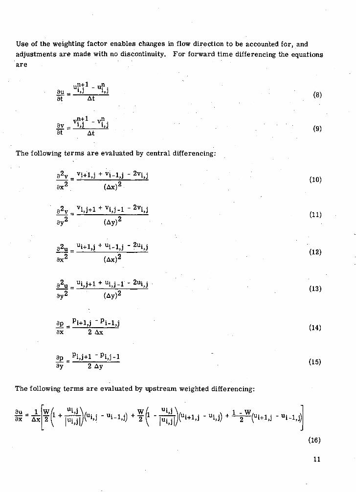
Use of the weighting factor enables changes in flow direction to be accounted for, andadjustments are made with no discontinuity. For forward time differencing the equationsare
au - ^Jat " At (8)
VP+1 - VPav ,at "" At (9)
The following terms are evaluated by central differencing:
8x
j-l,j -2VJJ
(Ax)(10)
(Ay)'(11)
(Ax)'(12)
(Ay)2 (13)
ax 2 Ax (14)
9y 2 Ay (15)
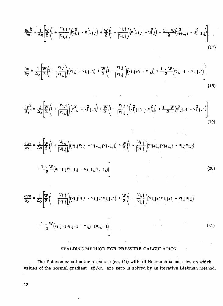
The following terms are evaluated by upstream weighted differencing:
9u _ 19x Ax f
(16)
11
ax Ax
3V _ 13y A
.
a v - l3y Ay
ffifl*
i - u2_l ,) + ? fl - 2 \ |ui,j
i - u
»AA.,. . v. . ,\ , Vff t Vi>J V,. . , v. .\ ," ^ " IJ+ " '^
< - u ! •
(17)
(18)
(19)
9uy _ 13x Ax ui iI 1>J
i i'J ui il'J- u
(20)
3vu _ 13y Ay
— [2 \
— Vi iI "I
i iu; i" 'J
— [2 \ ^
i i'Ji i+1 - vi i'J 'J
'j+1Ui'J+1 -vu-iuu-i) (21)
SPALDING METHOD FOR PRESSURE CALCULATION
The Poisson equation for pressure (eq. (4)) with all Neumann boundaries on whichvalues of the normal gradient 3p/3n are zero is solved by an iterative Liebman method.
12
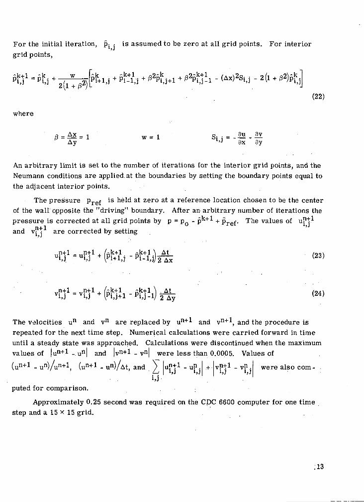
For the initial iteration, p=i
grid points,
is assumed to be zero at all grid points. For interior
where
(22)
Ayw = 1 i i>J
9uax
9v-ay
An arbitrary limit is set to the number of iterations for the interior grid points, and theNeumann conditions are applied at the boundaries by setting the boundary points equal to
the adjacent interior points.
The pressure pref is held at zero at a reference location chosen to be the centerof the wall opposite the "driving" boundary. After an arbitrary number of iterations the
The values ofpressure is corrected at all grid points byr»_i_ 1
and Vj t are corrected by settingp = P0 - p^"1"* + Pref.
At (23)
At (24)
The velocities un and vn are replaced by un+^ and vn+^, and the procedure isrepeated for the next time step. Numerical calculations were carried forward in timeuntil a steady state was approached. Calculations were discontinued when the maximumvalues of |un+l - un| and |vn+l - vn were less than 0.0005. Values of
- un were also com-(un+l _ un)/un+lj (un+l _ Un)/At> and
7<i
puted for comparison.
Approximately 0.25 second was required on the CDC 6600 computer for one timestep and a 15 x 15 grid.
RESULTS
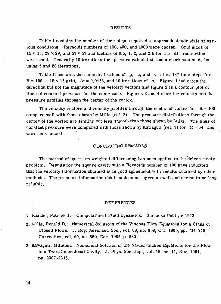
Table I contains the number of time steps required to approach steady state at var-ious conditions. Reynolds numbers of 100, 400, and 1000 were chosen. Grid sizes of15 x 15, 29 x 29, and 57 x 57 and factors of 0.5, 1, 2, and 2.5 for the At restrictionwere used. Generally 10 iterations for p were calculated, and a check was made byusing 5 and 20 iterations.
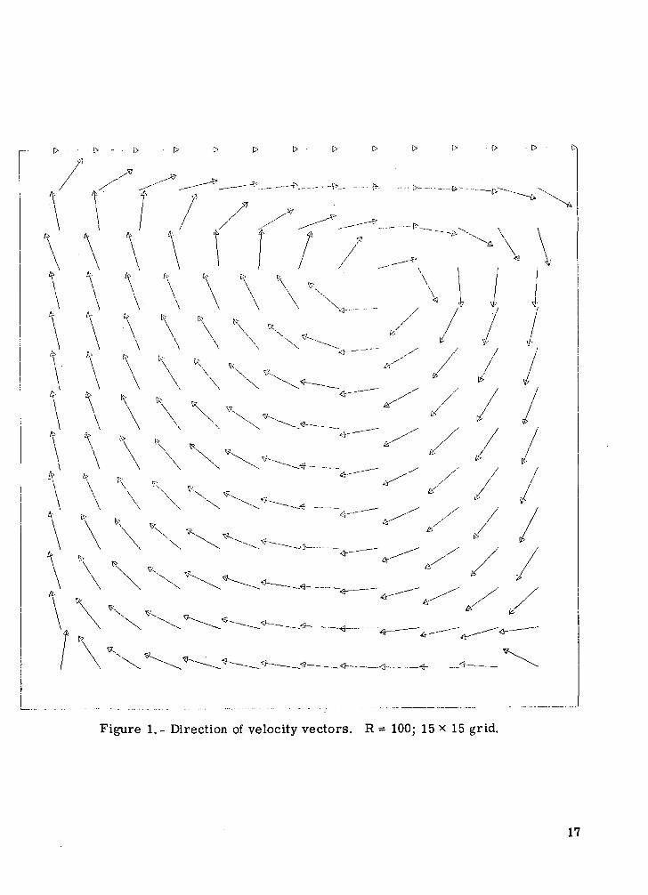
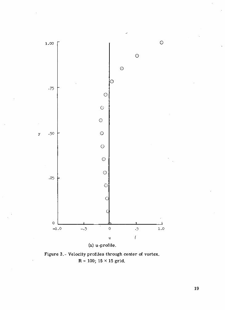
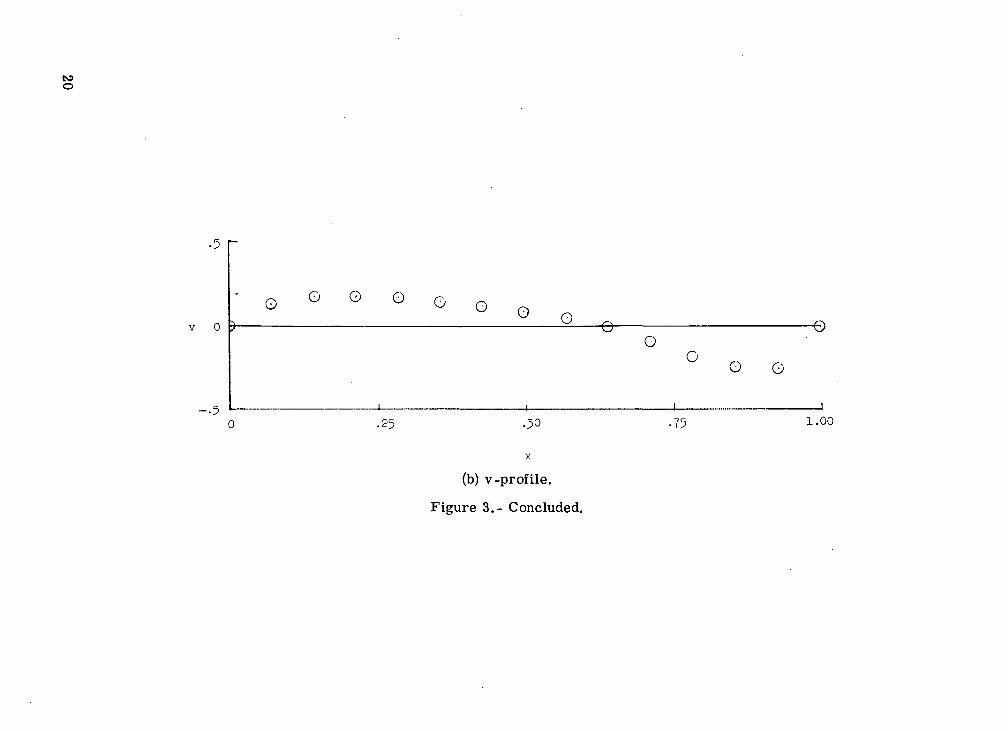
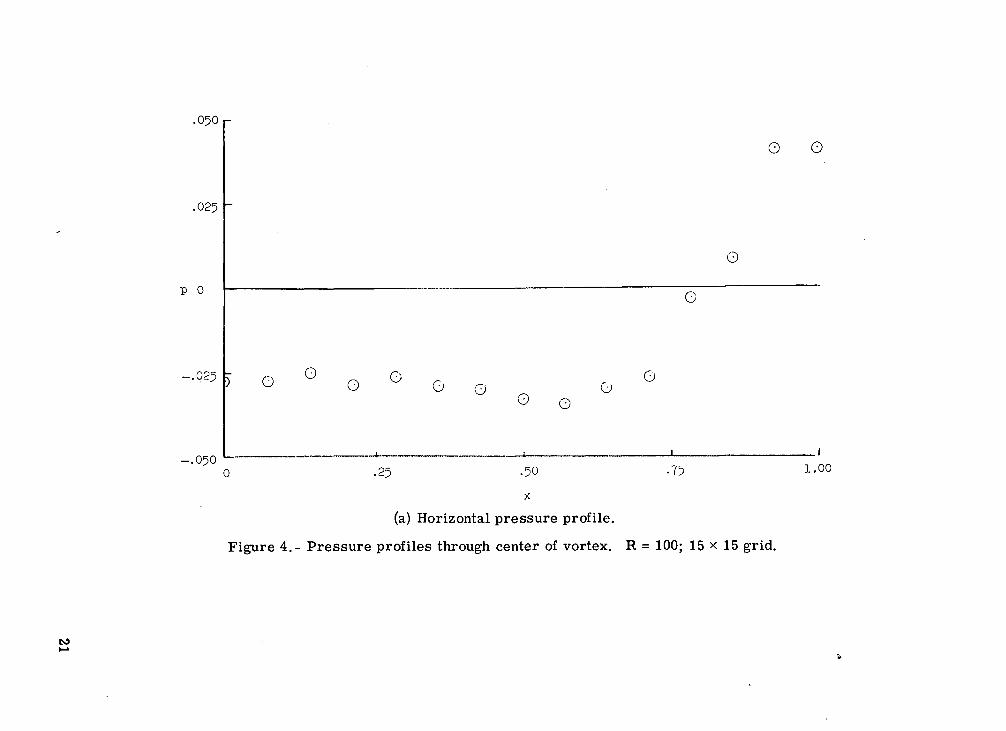
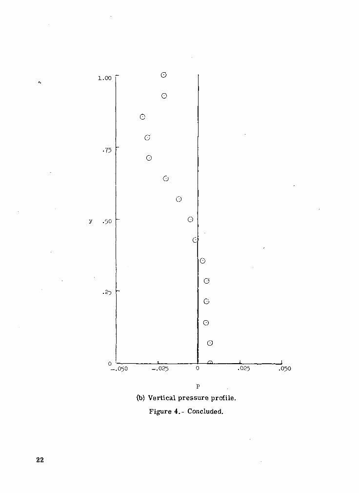
Table II contains the numerical values of p, u, and v after 187 time steps forR = 100, a 15 x 15 grid, At = 0.0458, and 10 iterations of p. Figure 1 indicates thedirection but not the magnitude of the velocity vectors and figure 2 is a contour plot oflines of constant pressure for the same case. Figures 3 and 4 show the velocity and thepressure profiles through the center of the vortex.
The velocity vectors and velocity profiles through the center of vortex for R = 100compare well with those shown by Mills (ref. 2). The pressure distributions through thecenter of the vortex are similar but less smooth than those shown by Mills. The lines ofconstant pressure were compared with those shown by Kawaguti (ref. 3) for R = 64 andwere less smooth.
CONCLUDING REMARKS
The method of upstream weighted differencing has been applied to the driven cavityproblem. Results for the square cavity with a Reynolds number of 100 have indicatedthat the velocity information obtained is in good agreement with results obtained by othermethods. The pressure information obtained does not agree as well and seems to be lessreliable.
REFERENCES
1. Roache, Patrick J.: Computational Fluid Dynamics. Hermosa Publ., c.1972.
2. Mills, Ronald D.: Numerical Solutions of the Viscous Flow Equations for a Class ofClosed Flows. J. Roy. Aeronaut. Soc., vol. 69, no. 658, Oct. 1965, pp. 714-718;Correction, vol. 69, no. 660, Dec. 1965, p. 880.
3. Kawaguti, Mitutosi: Numerical Solution of the Navier-Stokes Equations for the Flowin a Two-Dimensional Cavity. J. Phys. Soc. Jap., vol. 16, no. 11, Nov. 1961,pp. 2307-2315.
14
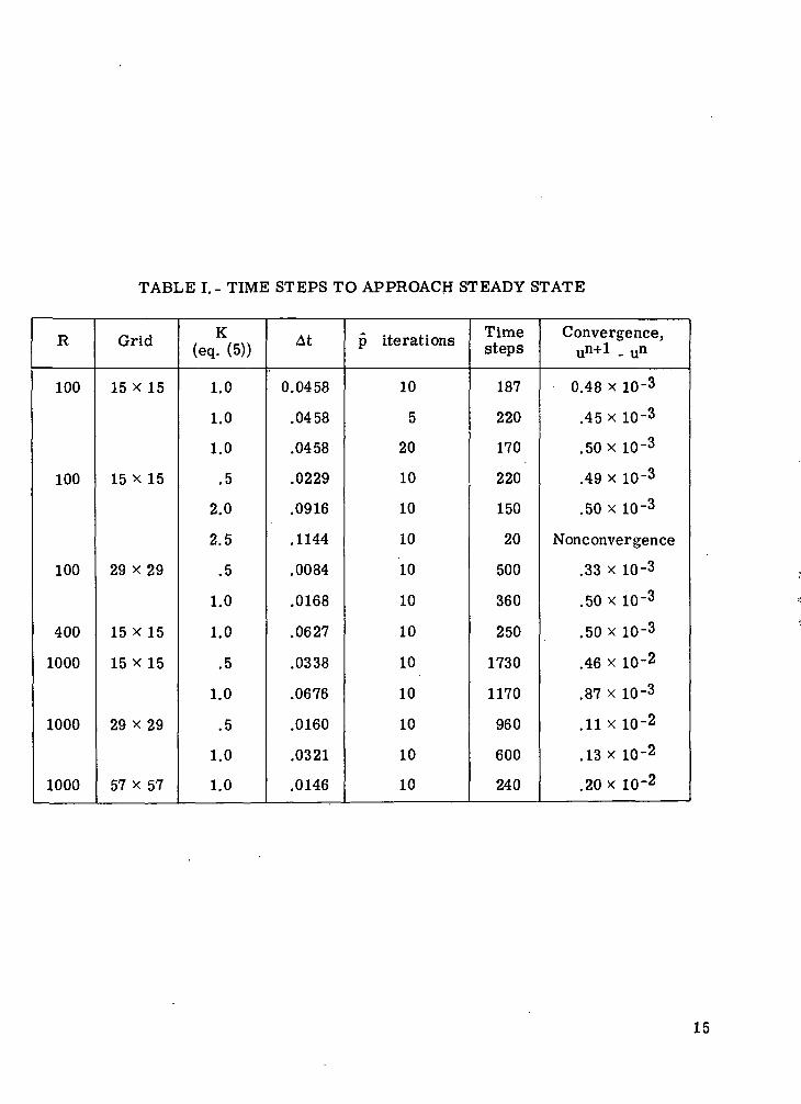
TABLE I.- TIME STEPS TO APPROACH STEADY STATE
R
100
100
100
400
1000
1000
1000
Grid
15 x 15
15 x 15
29 x 29
15 x 15
15 x 15
29 X29
57 x 57
(eq. (5))
1.0
1.0
1.0
.5
2.0
2.5
.5
1.0
1.0
.5
1.0
.5
1.0
1.0
At
0.0458
.0458
.0458
.0229
.0916
.1144
.0084
.0168
.0627
.0338
.0676
.0160
.0321
.0146
p iterations
10
5
20
10
10
10
10
10
10
10
10
10
10
10
Timesteps
187
220
170
220
150
20
500
360
250
1730
1170
960
600
240
Convergence,un+l _ un
0.48 x 10⁻³
.45 x 10-3
.50x 10-3
.49 x ID-3
.50x 10-3
Nonconvergence
.33 x 10-3
.50 x 10-3
.50x10-3
.46 x lO-2
.87 x 10-3
.11 x 10-2
.13 x lO-2
.20 x 10-2
15
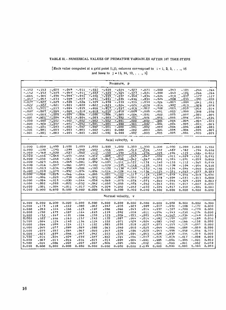
TABLE II.- NUMERICAL VALUES OF PRIMATIVE VARIABLES AFTER 187 TIME STEPS
[Each value computed at a grid point (i,j); columns correspond to i = 1, 2, 3, . . ., 15
and lines to j - 15, 14, 13, . . ., l]
Pressure, p
-.152-.152-.06*-.057-.027-.022-.011-.007"-.003-.001-.000-.000-.001-.001-.001
'
1.0000.0000.0000.0000.000u.ooo0.0000.0000.0000.0000.0000.000;).ooo0.0000.000
-.152-.152-.064-.057-.027-.022-.011-.007'-.003"-.001-.000-.000-.001-.001-.001
1.000.130
-.0*0-.056-.030-.023-.016-.013-.010-.008-.006-.00*-.002
.0010.000
-.025-."025-.036-.033-.025-.021-.013-.'00')-.005-.00*-.002-.002-.003-.003-.003
1.000.~i93
-.020-.065-.0*8-.0*"*-.037-.03*-.029-.025-.020-.015-.010-.00*0.000
-.0*9-.0*9"
---.o**-.039-.028-.021-.or*-.009-.005-.003-.002-.001-.002-.003-.003
1.000.289".023
-.053-.061-.065-.061-.058-.052-.0*6-.038-.030-.021-.0110.000
-.011-.Oil-.031
" -.027-.026-.020-.015- . 01 0"-.006-.00*-.002-.002-.002-.003-.003
1.000.3*0.060
-.0*1-.068-.081-.OS3-.081-.07*-.066-.055-.0**-.032-.0170.000
-.022"-.022-.036-.031-.029-.022-.016-.010-.006-.003-.002-.001-.002-.002-.002
1.000.*02.112
-.012-.065- . 092-. 102-.103-.096-.085-.072-.058-.0*2-.02*0.000
-.020" "-.020
-.035-.031 "-.030-.023-.017"-.010-.006-.003-.002-.001-.001-.001-.001
Axial
1.000.**6. 150.009
"-.063 '-. 103-.120-. 122-.11*-.101-.085-.069-.050-.0290.000
-.02* -.027-.02* "" -.027-.037 -.0*0-.03* -.036-.033 -.03*-.02* -.02*
"-".017 -~.6f6"-.Old" -".009-.005 -.00*-.002 -.001-.001 .000
.000 .001-.000 .0010.000 .0020.000 .002
velocity, u
1.000 1.000.*8* .512.190 .216.032 .0*3
'-.060 -.062-.111"" - .122"-.135 -.1*8-.138 -.1*9-.128 -.136-.112 -.117-.09* ' -.097-.075 -.076-.055 -.056-.032 -.0320.000 0.000
-.021-.021-.03*-.031-.030"-.020-.012-.005-.001
.001
.002
.002
.002
.003
.003
1 .000.526.23*.0*7
-.067-.T31-.155-.153-.136-.11*-.092-.071-.052-.0300.000
-.000-.000-.026-.02*-.026-.01*-.008-.001
.002
.003
.00*
.00*
.003
.005
.005
1.000.517.225.030
-.081-. 1*0-.155-. 1*6-.125-. 100-.078-.060-.0*3-.02*0.000
.0*3
.0*3
.010
.008-.003
.002
.003"".o'o's"
.005
.005
.00*loo*.00*.005.005
1.000.*87.20*.011
-.086-. 133-.139-.12*-.101-.078-.059-.0**-.031-.0170.000
. 101
.101" .037. 033.009".O"l3.010
".009.007.006.005.005.00*.006.006
1.000. 382.129
-.029-.091-.112-.10*-.08*-.063-.0*6-.033-.025-.017-.0100.000
.26* .26*
.26* .26*
.127 .127
.095 .095
.0*1 .0*1
.028 .023
.01* .01*
.008 .008_. 005 .005.00* .no*.003 .003.003 .003.003 .003.005 .005.005 .005
1.000 1.000.29* 0.000.08* 0.000
-.021 0.010-.059 0.000-.065 0.010-.05* 0.000-.0*0 0.000-.027 O.OOJ-.013 0.000-.013 0.000-.009 O . O O J-.007 0.030-.00* 0.0000.000 0.000
Normal velocity, v
0.0000.0000.0000.0000.0000.0000.000o.ooou.oooo.ooo0.000"6 .Too"0.000o.oooo.ooo
0.000.173.203.150.132.10?.084.06*.0*9.035.023.01*.007.00*
0.000
0.000. 118. 16*.179. 167.1*6.12*.099.077.057.039.02*.013.006
0.000
0.000.112. 166. 187.181.163.1*0. 11*.089.066.0*6
".029.016.007
0.000
0.000.080.125.16*.166.157.136.113.089.067.0*7.030.016.007
0.000
0.000.062.107.1*5.150.1*3. 12*. 102.080.060.0*2".027.015.007
0.000
0.000.0*7.086. 119. 125. 120. 102.083.063.0*7.033.022.013.006
0.000
0.000 0.000.035 .023.066 .0*3.092 .058.09* .053.087 .0**.071 .029.055 .018.0*0 .010.029 .006.0"20 .00*.01* .00*.009 .00*.005 .00*
0.000 0.000
0.000.009.01*.011
-.003-.01*-.02*-.027-.025-.020-.013-.007-.001
.0020.000
0.000-.017-.037-.05*-.076-.082-.083-.073-.059-.0*3-.028-.015-.005.001
0.000
0.000-.051-.!07-.1*3-. 167-.159-.1*2-.115-.086-.059-.037-.019-.006
.0000.000
0.000-.108-.200-.230-.236-.202-.166-.125- .08fi-.058-.03*-.017-.005
.0010.000
0.000 0.000-.172 0.000-.279 0.000-.27* 0.000-.2*9 0.000-.189 0.000-.138 0.000-.09? 0.000-.059 0.000-.036 0.013-.019 0.000-.008 0.000-.001 0.000
.002 0.0000.000 0.000
16
[ > - - ! > - • [ > [> [> [> O
Figure 1.- Direction of velocity vectors. R = 100; 15 x 15 grid.
17
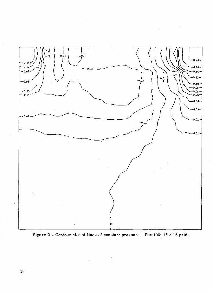
Figure 2.- Contour plot of lines of constant pressure. R = 100; 15 x 15 grid.
18
1.00
• 75
y .50
.25
0
O
G
O
O
O
O
O
G
G
c
1 /
e
0
0
o
•N 1 1
-1.0 -5 • 5 1.0
(a) u-profile.
Figure 3.- Velocity profiles through center of vortex.R = 100; 15 x 15 grid.
19
r.
O©0o00oo
J '
f }
O0o
o)
-
\ir>
o u
{-JHir\c—
•O<v•o3m
>— *0
X
0
">
*
Jg
gS
oai
'>
eo
a 231fe
mOJ0
-\l"
20
oo
o
1 1
-
o
o
0
ooo0
0•
oool/~\
00M
T3'CfaninT-l
Xmi— t
ir\ •-
t- OOi-HII
tf
*' si
._ <D
*t; •+->
O
^ti
Oa
>2
oo
5 ^
^
x
M 5
<u n
e.
*j\
M
Va
orj
-C1 3
0
§
I
•^
F*— 1
^
-l->O
tn
t..
UJ
K
0i— i
3 ?
ITN
^HO
J Q
<
Q)
hcoCQcut .MOn'.
_M*J^
0)&-C
s,1
= S
O
ITv
ITN
O
S
8 2 -
&ft
i' f
21
1.00
•75
y .50
•25
0
u
0
G
G
O
G
G
O
G
-
i
G
G
G
0
O
r\ l 1
.050 -.025 o .025 .(
(b) Vertical pressure profile.
Figure 4.- Concluded.
22
3. SOLUTION OF THE INCOMPRESSIBLE DRIVEN CAVITY PROBLEM
USING THE CROC CO METHOD
Jerry N. HefnerLangley Research Center
SUMMARY
The Crocco method has been used to solve the steady Navier-Stokes equations fortwo-dimensional flow in a square driven cavity for a Reynolds number of 100. TheThe Spalding SIMPLE procedure was used to solve the pressure-linked equations.Results for velocity and pressure were found to be inaccurate, although the overallrecirculation and vortex center were correctly predicted.
INTRODUCTION
During the past decade, the evolution of large high-speed computers has allowedthe development of numerous explicit and implicit finite ^difference schemes for solvingthe steady Navier-Stokes equations. In general, these numerical procedures have notbeen rigorously tested on a variety of problems. Consequently, .the value of a givenmethod for solving a multiplicity of fluid dynamics problems often has not been ascer-tained. In this paper, results of a numerical study to predict the velocity profiles andpressure distribution in the simple two-dimensional driven cavity with width-depth ratioof 1 (square cavity) and Reynolds number of 100 are presented. (See paper no. 1 byRubin and Harris for details of driven cavity problem.) The method used is that attri-buted to Crocco (ref. 1) with the Spalding SIMPLE procedure (ref. 2) for solving thepressure-linked equations.
SYMBOLS
I width of cavity
AZ spatial increment in x and y
p pressure
p error in pressure (eq. (9))
P0 initial estimate of p
23
q actual velocity vector
q* calculated velocity vector (eq. (9))
R Reynolds number,v
t time
At time step
U velocity in x-direction at edge of cavity
u velocity in x-direction
v velocity in y-direction
x,y axial and normal coordinate of cavity, respectively
r variable used in equations (5) to (8)
17 viscosity
p density
w variable in successive overrelaxation method given in equation (12)
Superscripts:
k iteration number
n time step number
Subscripts:
i step in x-direction
j step in y-direction
24
x,y
differentiation with respect to time
differentiation with respect to x or y
Bars over symbols denote dimensional quantities.
METHOD OF ANALYSIS
The nondimensional viscous incompressible flow equations in primitive variablesare
UX + Vy = 0
UUX + VUy_ 1
i(UxX + Uyy)
(1)
(2)
VVy 'yy> . (3)
The variables have been nondimensionalized with respect to U and I; that is,
P *_«P =PU2 I
U (4)U
I
The boundary conditions are as follows:
aty = 0 u = v = 0
at y = 1 u = 1 and v = 0
atx = 0 u = v=0
atx = l u = v = 0
The Grocco method (ref. 1) was applied to the x- and y-momentum equations (eq. (2)and (3), respectively) to solve for velocities u and v. The method presented by Crocco
25
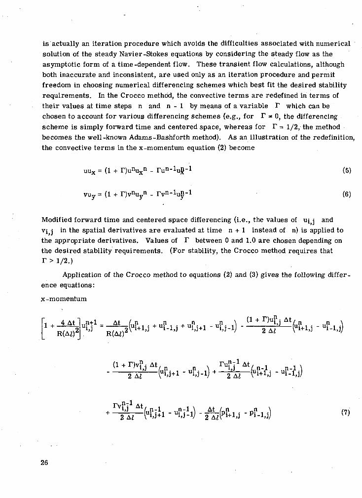
is actually an iteration procedure which avoids the difficulties associated with numericalsolution of the steady Navier -Stokes equations by considering the steady flow as theasymptotic form of a time -dependent flow. These transient flow calculations, althoughboth inaccurate and inconsistent, are used only as an iteration procedure and permitfreedom in choosing numerical differencing schemes which best fit the desired stabilityrequirements. In the Crocco method, the convective terms are redefined in terms oftheir values at time steps n and n - 1 by means of a variable F which can bechosen to account for various differencing schemes (e.g., for F a 0, the differencingscheme is simply forward time and centered space, whereas for F = 1/2, the methodbecomes the well-known Adams -Bashforth method). As an illustration of the redefinition,the convective terms in the x -momentum equation (2) become
uux = (1 + F)unuxn - ru11-^-1 (5)
vuy= (1 + F)vnuyn - Fv11-^-1 (6)
Modified forward time and centered space differencing (i.e., the values of uy andvij in the spatial derivatives are evaluated at time n + 1 instead of n) is applied tothe appropriate derivatives. Values of F between 0 and 1.0 are chosen depending onthe desired stability requirements. (For stability, the Crocco method requires that
Application of the Crocco method to equations (2) and (3) gives the following differ-ence equations:
x-momentum
1+-1AL uf ! , + uf , - u \- j un nI~1»3 l> '
(1 + F)vni At, n _ N Fu' 1»] /nn. n. \ .-- 2~Al - V l'J+1 " l 'J-V
1 At
F v y A t , x
26
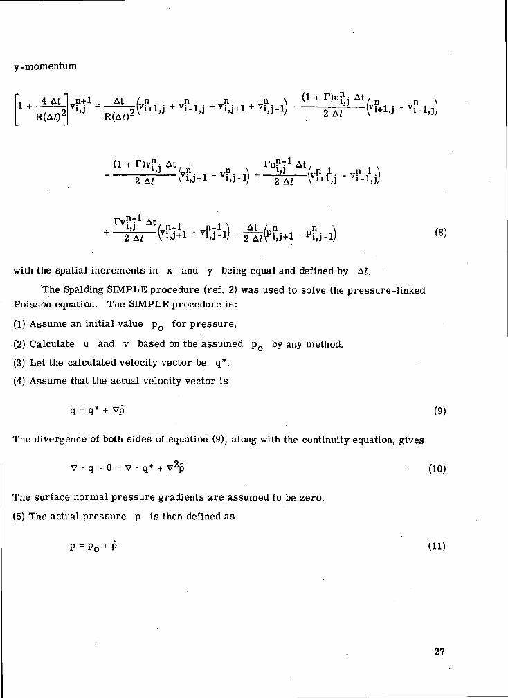
y-momentum
4 At1 "± AIL •trJ*TJL — tiL fv" . _L Tfi1 _L T/.1 . j_ TrP \
At r,,"-ln. \ Y>J n
with the spatial increments in x and y being equal and defined by AZ.
The Spalding SIMPLE procedure (ref. 2) was used to solve the pressure -linkedPoisson equation. The SIMPLE procedure is:
(1) Assume an initial value po for pressure.
(2) Calculate u and v based on the assumed po by any method.
(3) Let the calculated velocity vector be q*.
(4) Assume that the actual velocity vector is
q = q* + Vp (9)
The divergence of both sides of equation (9), along with the continuity equation, gives
V - q = 0 = V - q * + V2p (10)
The surface normal pressure gradients are assumed to be zero.
(5) The actual pressure p is then defined as
(ID
27
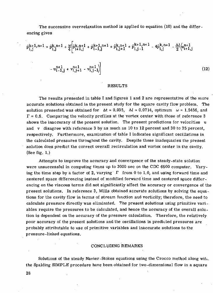
The successive overrelaxation method is applied to equation (10) and the differencing gives
k+l,n+l = k,n+l +
,, n-t-1+ vy+1 -vy.ij
RESULTS
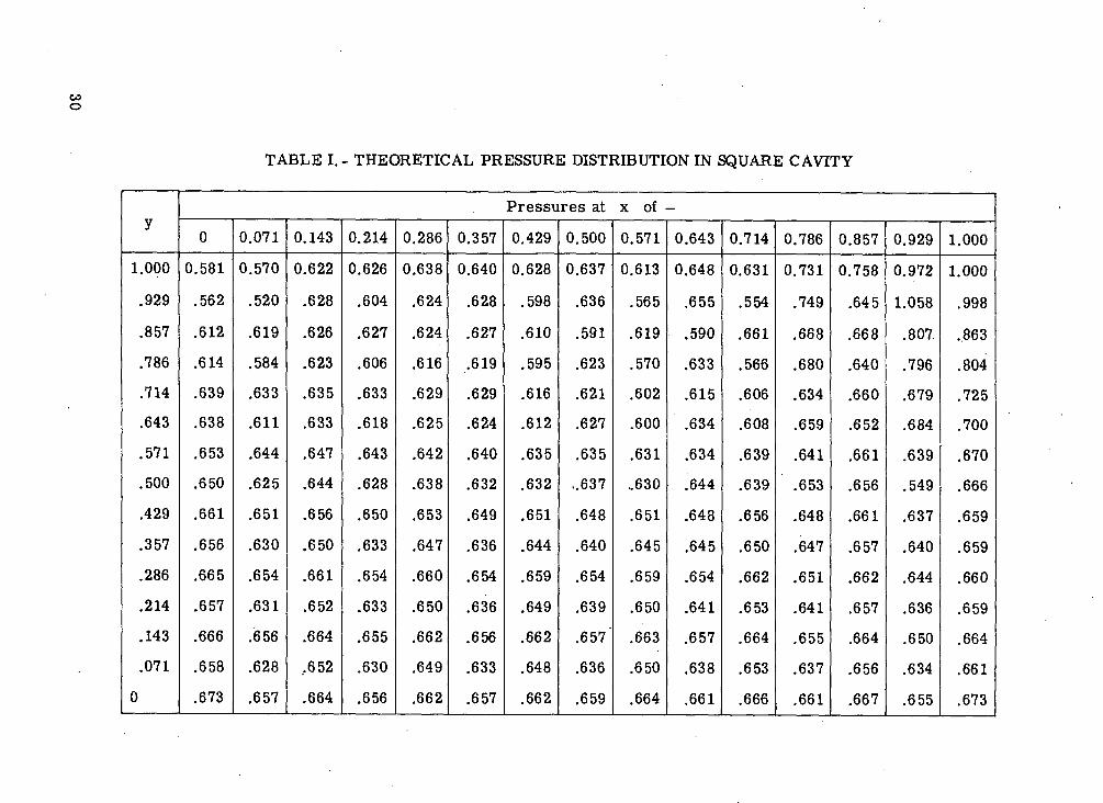
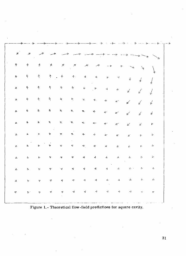
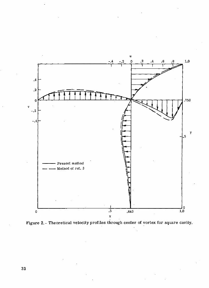
The results presented in table I and figures 1 and 2 are representative of the moreaccurate solutions obtained in the present study for the square cavity flow problem. Thesolution presented was obtained for At = 0.035, AZ = 0.0714, optimum w = 1.5456, andF = 0.6. Comparing the velocity profiles at the vortex center with those of reference 3shows the inaccuracy of the present solution. The present predictions for velocities uand v disagree with reference 3 by as much as 10 to 12 percent and 30 to 35 percent,respectively. Furthermore, examination of table I indicates significant oscillations inthe calculated pressures throughout the cavity. Despite these inadequacies the presentsolution does predict the correct overall recirculation and vortex center in the cavity.(See fig. 1.)
Attempts to improve the accuracy and convergence of the steady-state solutionwere unsuccessful in computing times up to 3000 sec on the CDC 6600 computer. Vary-ing the time step by a factor of 2, varying F from 0 to 1.0, and using forward time andcentered space differencing instead of modified forward time and centered space differ-encing on the viscous terms did not significantly affect the accuracy or convergence of thepresent solutions. In reference 3, Mills obtained accurate solutions by solving the equa-tions for the cavity flow in terms of stream function and vorticity; therefore, the need tocalculate pressure directly was eliminated. The present solutions using primitive vari-ables require the pressures to be calculated, and hence the accuracy of the overall solu-tion is dependent on the accuracy of the pressure calculation. Therefore, the relativelypoor accuracy of the present solutions and the oscillations in predicted pressures areprobably attributable to use of primitive variables and inaccurate solutions to thepressure-linked equations.
CONCLUDING REMARKS
Solutions of the steady Navier-Stokes equations using the Crocco method along wituthe Spalding SIMPLE procedure have been obtained for two-dimensional flow in a square
28
driven cavity. The results for the axial and normal velocities did not agree with thoseof another accurate method, and significant pressure oscillations were noted. Theseinadequacies were probably due to use of primitive variables and to inaccurate solutionsto the pressure-linked equations. The solution did correctly predict the overall recir-culation and vortex center.
REFERENCES
1. Crocco, Luigi: A Suggestion for the Numerical Solutions of the Steady Navier-StokesEquations. AIAA J., vol. 3, no. 10, Oct. 1965, pp. 1824-1832.
2. Caretto, L. S.; Gosman, A. D.; Patanker, S. V.; and Spalding, D. B.: Two CalculationProcedures for Steady, Three-Dimensional Flows With Recirculation. Rep.No. EF/TN/A/47, Dep. Mech. Eng., Imperial College Sci. & Technol., June 1972.
3. Mills, Ronald D.: Numerical Solutions of the Viscous Flow Equations for a Class ofClosed Flows. J. Roy. Aeronaut. Soc., vol. 69, no. 658, Oct. 1965, pp. 714-718;Correction, vol. 69, no. 660, Dec. 1965, p. 880.
29
o0oi-H
O>CM05Ot-inCOoCOoot>o•*T-4t-oCO•*coo
«_ r-i
O
t-LO
X 0
•y o
rt o
to «
2 °
2W
OS
CQ CM
cu >*
fi _£jt-mCOoCDCOCM
o•*1— (CMOCO•*I— 10I— 1c-ooo
>>
ooo1— (
CM1>O5
OCOmc-0T-ICOt-0r-lCOCD
OCO
•<*CO
oCO
1-1CD
0c-coCO0COCMCDOOTfCDOCOCOCO
0coCMCDOCMCMCO
o0t>moiHCO\f)
0ooo1— 1
CO0505
coino.-iin•CDO5
•t*r-
smminCO
incomCDCOCD
CO05incoCMCO
•*CXICD
•0CD
CO<NCD
0CMinCNCOinO5CMOS•
COCDCO
I>ocoCOCOCO
COCDcoi-HCOcooO5m05»HCO
tH05inoj— tcot-CMCO
•* -CMCD
c-CMCOCDCMCO
05
i— 1CO
CMT-{
CO
c-inco
• -0COCOO5
ir-O•CO
OCOCO
cocoinCOCOcooc-mCOCMCD
mO5inO5
V- (
CD
CD
1— t
CO
co0CDCO
CXICD
•COin•1-1CD
COCOD-*
in o
CM
Or-
t-
OS
TJIt-
CO
co co
O CM
CD m
CO
CO
•5*1 OS
co m
co co
SCO0
co co
in ^
i-H CO
CO
CO
CM 0
o o
CO
CD
i-c tr-
(M
CMCO
CO
CD
CMr-l
i-lCO
CO
O5
T}<CM
CM
co co
os m
CM
CM
CD
CO
CO
CO
CO
i-lCO
CO
in co
CO
CO
CO
CO
CO
j-tCO
i-(CO
CO
os co
CO
CO
CD
CD
•
CO
r-l ^
C-
CD
O CD
C-
CDCD
CO
O5
OS
CO
rf
co in
i— 1 CO
CD m
CO
CO
r-l
CO
TJ< in
CD
CD
05
OS
CO
CO
CD
CO
•* •*
CO
•sjlCD
CD
i-H O
CO
CO
CO
CO
in f-
CO
CO
CO
CO*
in CM
CO
CO
CD
CO
O CM
•SF CO
CD
CO
CM
CO
Tj< CO
CO
CO
CO
CO
•<*< CM
co co
c- ^
•
Tl<CO
CO
•
inTJ<
CMCD
CD
CO
Oin
inco
co
i-l O
C- O
in in
osinCO
t-cocor-lCDCDCO
•<*<co£coCO•CD
1— IinCDco•*CDi-HinCD05•*COCOmcooinCO
8CD
1— IinCD1— 1CDCDOS
CM•*
05 O
in CD
CD
CO
O T)<
Tj<
TJ(
CD
CO
t-
CMin
CDCD
CO
t- 1-1
•t 1 m
.CD
CO
O CM
in CD
CD
CD
in TJ<
• m
CO
CD
in os
TJ< in
CD
CO
o ^
•
inco
co
•*
OS
•
inCO
CO
CD -<1<
co in
co co
t- o
•st 1 co
CD
CO
CO
<co
inco
co
O i-l
in co
CO
CO
O T}(
co m
CO
CD
co m
in CD
co co
t- co
m co
CO
CM
05inCOCDCOCO
t-mCDi— i•CDCOmCDr-l
-*CO
OinCO
OSCOCD
O5•*COcoCOcooinCD
COCOCD
CMincor- 1COCD
c-inCD•
•*r-lCM
•<*CDCD
0inCD•CDCD
inmCO<*COCOt>incoCOcocot~inCDCMcoCO8coCMcocoininCO
•sf 1
COcoCOin.CO
coCOCDCO
tH
r-t CO
co t-
CO
CD
TJ< in
co m
co co
co t-
in CD
co co
I>
i-HCO
CD
co co
co co
in CD
CD
CD
co 1-1
CO
CD
CD
CD
O 'I*
in CD
co co
CD
OS
co in
CD
CO
CO
CM
•*
CD
CO
CD
CO
t-
co in
co co
OS
CM
-* co
CD
CO
O CD
co m
co co
CM
-m co
CD
CO
co r-
CM in
CO
CO
CO
CO
in c-
CO
CO
1— 1c-o
o
30
f>
--—fc.A
S»
/ /
v V
>' tf
Figure 1.- Theoretical flow-field predictions for square cavity.
4
A &.
31
-.4 -.2 0 .2 .4 .6 .8
Present methodMethod of ret. 3
1.0
Figure 2.- Theoretical velocity profiles through center of vortex for square cavity.
32
4. SOLUTION OF THE DRIVEN CAVITY PROBLEM IN
PRIMITIVE VARIABLES USING THE SMAC METHOD
Richard S. HirshLangley Research Center
SUMMARY
The equations of two-dimensional incompressible fluid flow in the driven cavityhave been solved in terms of primitive variables. The Simplified Marker-and-Cellmethod was used with forward time and centered space (FTCS) differencing and withmodified forward time and centered space (MFTCS) differencing. The problem couldnot be solved for a Reynolds number of 100 with FTCS differencing because of stabilitylimitations. For a Reynolds number of 10, the results were found to be inaccuratebecause of the inability of the pressure solver to converge to small tolerances. TheMFTCS differencing seemed to relax the stability restriction on time step, but the limiton cell Reynolds number was retained. A lower order boundary condition on pressureresulted in marginal improvement.
INTRODUCTION
The equations of two-dimensional incompressible fluid flow can be integrated byeither of two general procedures. The equations can be utilized as they are, writtenexpressing conservation of mass and momentum in terms of axial and normal velocityand pressure, that is, the so-called primitive variables (PV); or the continuity equationcan be satisfied by a stream function, and the pressure can be eliminated by taking thecurl of the momentum equations to yield the vorticity—stream-function (VSF) system.
The VSF system is attractive since it reduces the number of equations from threeto two and eliminates the troublesome continuity equation. This gain is offset somewhatby the difficulties encountered when dealing with the unknown boundary conditions onvorticity. In some problems, such as aerodynamic flows, for which knowledge of thepressure is desired, the VSF system must be supplemented by additional relations forthe pressure. The PV system, on the other hand, yields the pressure directly and haslittle difficulty with the boundary conditions. The present study considers the solutionof the driven cavity problem with a method which solves the PV system, and results arecompared with a solution of the VSF system. See paper no. 1 by Rubin and Harris fordetails of the driven cavity problem.
33
SYMBOLS
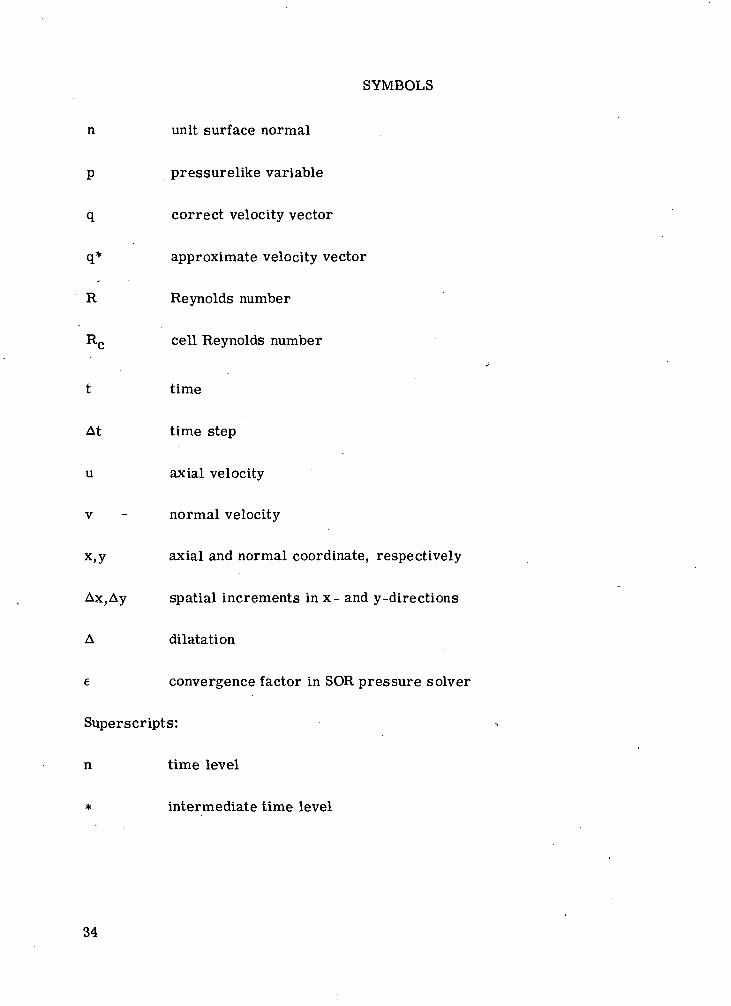
n unit surface normal
p pressurelike variable
q correct velocity vector
q* approximate velocity vector
R Reynolds number
Rc cell Reynolds number
t time
At time step
u axial velocity
v - normal velocity
x,y axial and normal coordinate, respectively
Ax,Ay spatial increments in x- and y-directions
A dilatation
e convergence factor in SOR pressure solver
Superscripts:
n time level
* intermediate time level
34

Subscripts:
i,j index of grid points in x- and y-direction, respectively
x,y,t differentiation with respect to x, y, or t
Abbreviations:
ADI alternating direction implicit
FTCS forward time and centered space
MAC Marker and Cell
MFTCS modified forward time and centered space
SMAC Simplified Marker and Cell
SOR successive overrelaxation
METHOD OF SOLUTION
The momentum equations in two-dimensional incompressible flow, written indimensionless divergence form, are (ref. 1)
ut + (u2)x + (uv)y = -px + l(Uxx + uyy) (1)
yy) (2)
The continuity equation is
A = ux + vy = 0 (3)
These three equations constitute the governing equations of the driven cavity problem.
The method of solution used is the Simplified Marker-and-Cell (SMAC) methodoriginally proposed by Amsden and Harlow. (See ref. 2.) Although this method does notyield the true pressure from the solution, it gives an indication of the accuracy which can
35
be achieved with the equations in terms of primitive variables since the velocity is cor-rect, as pointed out in reference 2.
The methodology of the SMAC method is as follows:
(1) Integrate the momentum equations one time step to generate an approximatevector solution q*.
(2) Knowing this to be incorrect since in general, it does not satisfy zero dilatation,assume that a pressurelike variable p corrects q* to the actual value q such thatdiv q = 0. Thus, say
q = q* + grad p (4)
(3) Since div q = 0, equation (4) gives
V2p = -div q* (5)
(4) Since q = q* on the boundaries, equation (4) gives for boundary conditions,
an (6)
(5) Once the Poisson equation (5) for the "pressure " is solved, the correct valueof q at this particular time step can be found from equation (4). Then, the whole pro-cess is begun again at step (1) and continued in time until two consecutive time stepshave velocities which differ by no more than some small convergence factor.
Note that the variable p is not the real fluid pressure, since the boundary condi-tion (eq. (6)) is not correct. The true normal conditions on the pressure can be derivedfrom equations (1) and (2) written at the wall.
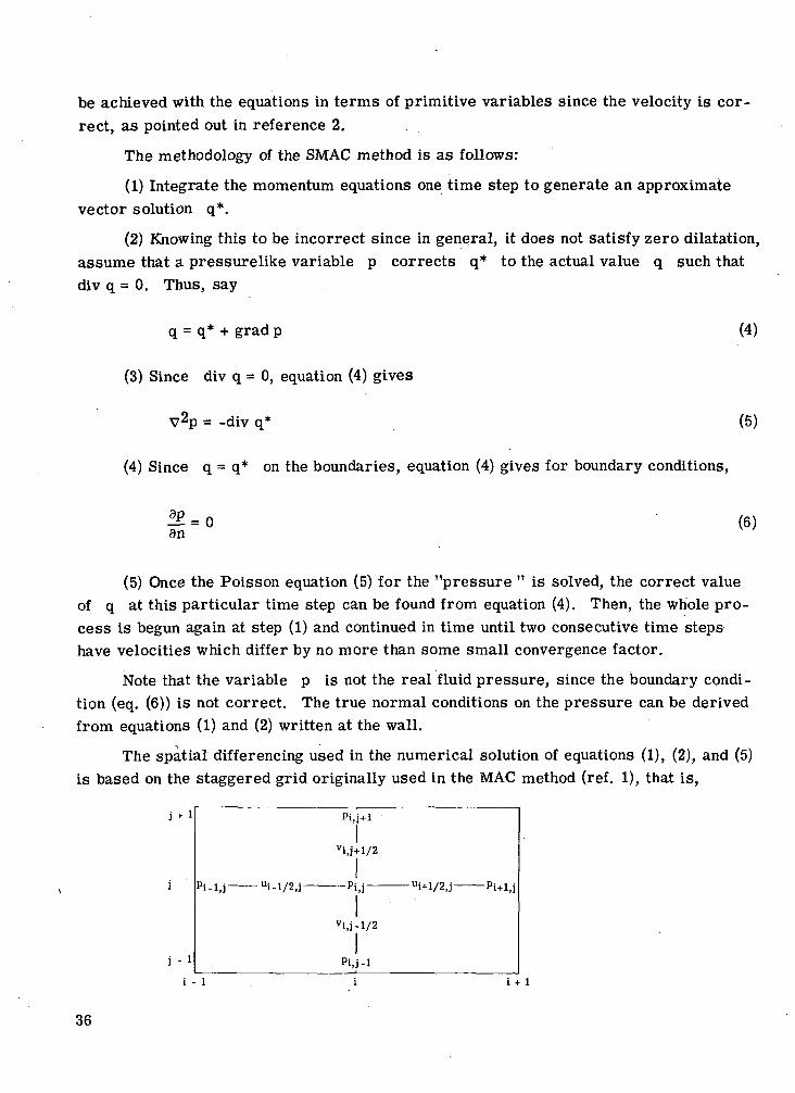
The spatial differencing used in the numerical solution of equations (1), (2), and (5)is based on the staggered grid originally used in the MAC method (ref. 1), that is,
j -
pi-l,j- -ui-l
Pi,3+l
Ivi,3+l/2
—pu—
vi,j-l/2
Pi,j-li - 1 i + 1
36
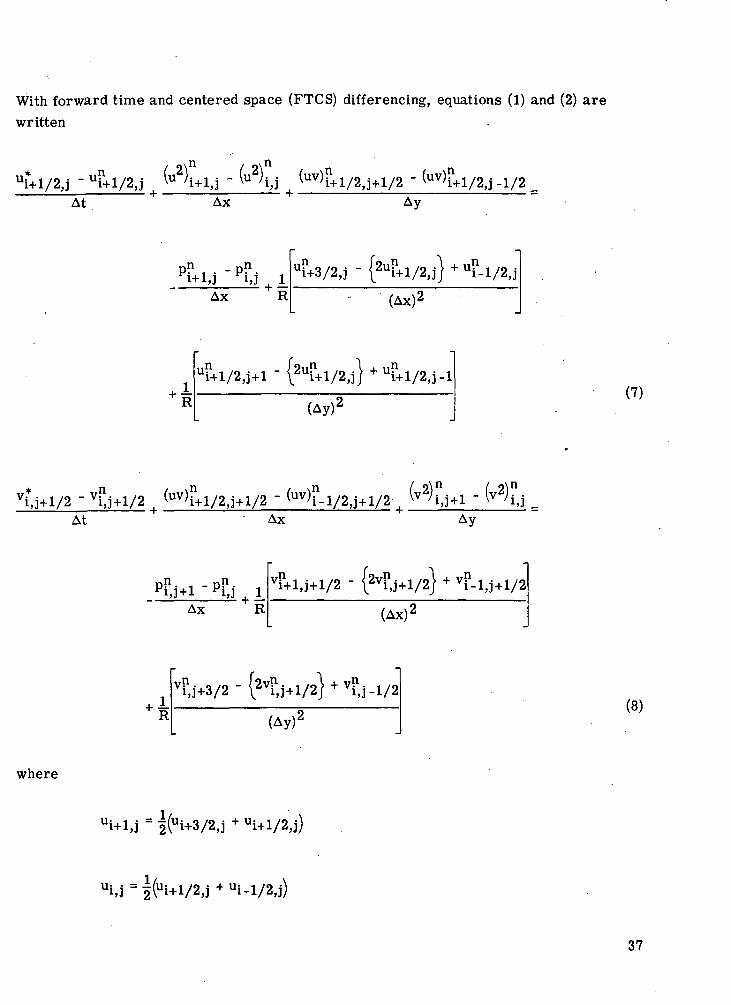
With forward time and centered space (FTCS) differencing, equations (1) and (2) arewritten
At
n(uv)iW2,j+l/2 ,j -1/2 _
Ax Ay
where
n - n
Ax,
R
u?+3/2,j
(Ax)2
(Ay)'(7)
At Ax
Ax R (Ax)'
(Ay)'(8)
37
, J+l
'i,M/2)
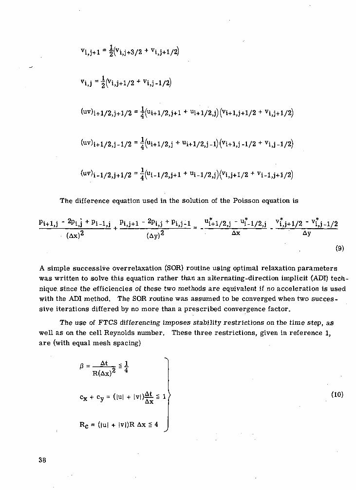
The difference equation used in the solution of the Poisson equation is
"J-1/2J
(Ax)' (Ay)' Ax Ay
(9)
A simple successive overrelaxation (SOR) routine using optimal relaxation parameterswas written to solve this equation rather than an alternating-direction implicit (ADI) tech-nique since the efficiencies of these two methods are equivalent if no acceleration is usedwith the ADI method. The SOR routine was assumed to be converged when two succes-sive iterations differed by no more than a prescribed convergence factor.
The use of FTCS differencing imposes stability restrictions on the time step, aswell as on the cell Reynolds number. These three restrictions, given in reference 1,are (with equal mesh spacing)
R(Ax)2 4
RC = (lu| + lv|)R Ax i 4
(10)
38
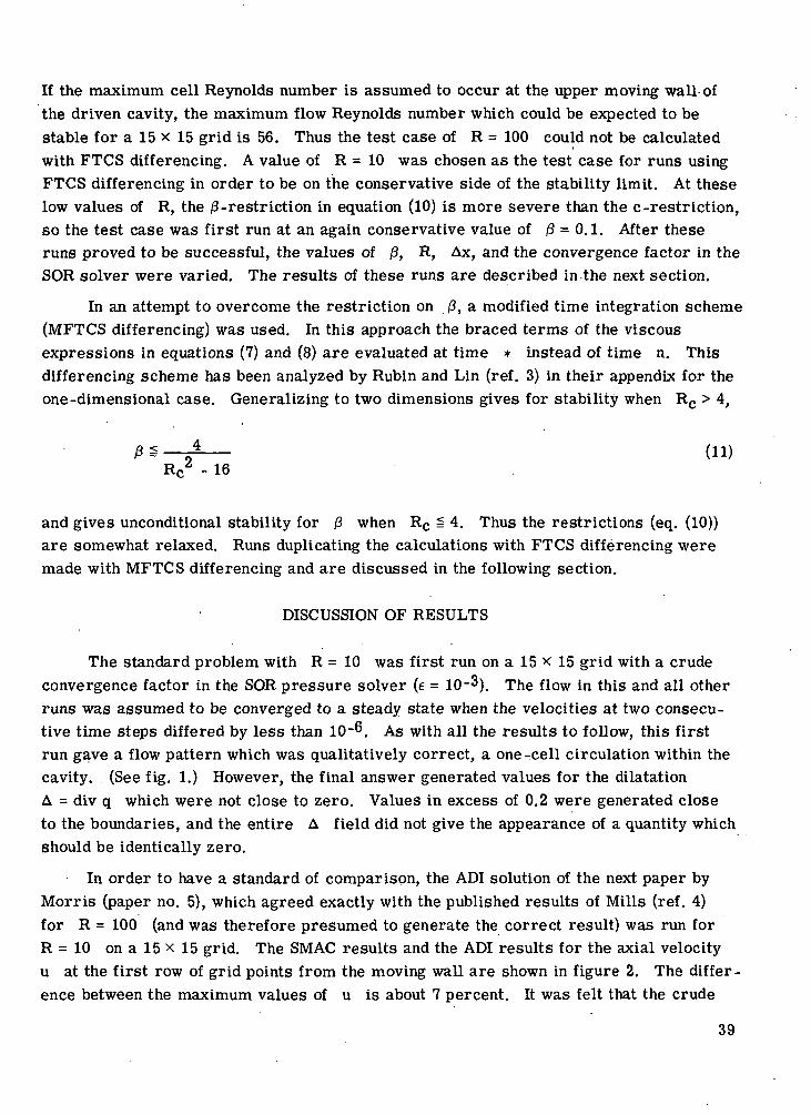
If the maximum cell Reynolds number is assumed to occur at the upper moving wall ofthe driven cavity, the maximum flow Reynolds number which could be expected to bestable for a 15 x 15 grid is 56. Thus the test case of R = 100 could not be calculatedwith FTCS differencing. A value of R = 10 was chosen as the test case for runs usingFTCS differencing in order to be on the conservative side of the stability limit. At theselow values of R, the /3 -restriction in equation (10) is more severe than the c -restriction,so the test case was first run at an again conservative value of /3 = 0.1. After theseruns proved to be successful, the values of )3, R, Ax, and the convergence factor in theSOR solver were varied. The results of these runs are described in the next section.
In an attempt to overcome the restriction on /3, a modified time integration scheme(MFTCS differencing) was used. In this approach the braced terms of the viscousexpressions in equations (7) and (8) are evaluated at time * instead of time n. Thisdifferencing scheme has been analyzed by Rubin and Lin (ref. 3) in their appendix for theone -dimensional case. Generalizing to two dimensions gives for stability when Rc > 4,
RCZ - 16
and gives unconditional stability for /3 when Rc = 4. Thus the restrictions (eq. (10))are somewhat relaxed. Runs duplicating the calculations with FTCS differencing weremade with MFTCS differencing and are discussed in the following section.
DISCUSSION OF RESULTS
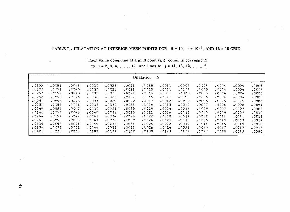
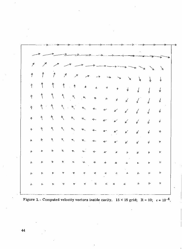
The standard problem with R = 10 was first run on a 15 x 15 grid with a crudeconvergence factor in the SOR pressure solver (e = 10~3). The flow in this and all otherruns was assumed to be converged to a steady state when the velocities at two consecu-tive time steps differed by less than 10~6. As with all the results to follow, this firstrun gave a flow pattern which was qualitatively correct, a one -cell circulation within thecavity. (See fig. 1.) However, the final answer generated values for the dilatationA = div q which were not close to zero. Values in excess of 0.2 were generated closeto the boundaries, and the entire A field did not give the appearance of a quantity whichshould be identically zero.
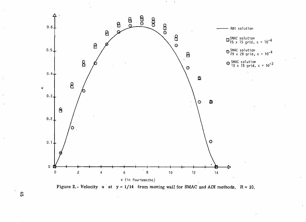
In order to have a standard of comparison, the ADI solution of the next paper byMorris (paper no. 5), which agreed exactly with the published results of Mills (ref. 4)for R = 100 (and was therefore presumed to generate the correct result) was run forR = 1 0 o n a ! 5 x i 5 grid. The SMAC results and the ADI results for the axial velocityu at the first row of grid points from the moving wall are shown in figure 2. The differ-ence between the maximum values of u is about 7 percent. It was felt that the crude
39
convergence for the pressure might lead to inaccuracies in the velocities (through thepressure gradients in the momentum equations), so the convergence factor for pressurewas lowered an order of magnitude to e = 10-4, an(j the identical problem was run again.The computation time was increased by a factor of 2.5, but the converged dilatation field,listed in table I, was considerably improved. There was a favorable change in all thevelocities as shown in figure 2. Now the difference between maxima was only4.5 percent.
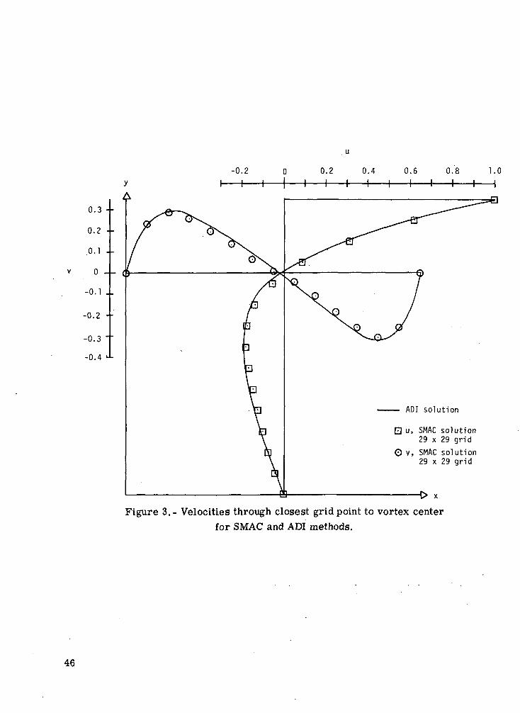
Since the accuracy of the pressure calculation seemed crucial, the SOR conver-gence factor was decreased another order of magnitude to e = 10 ~5. With this value theSOR pressure solver would not converge. It was then decided to use e = 10-5 but to cutoff the iteration at a large arbitrary limit (1000 iterations) if the convergence was notfulfilled and proceed to the next time step. The result was a significantly more uniformdilatation field. However the typical value of dilatation computed, 0.0040, was no betterthan the value for e = 10"4 (table I). Thus, it seems that in addition to being the mosttime-consuming segment of the calculation, the method used for the pressure solver con-trols the overall accuracy of the computation. A plot of the velocity vector field fore = 10-^ is presented in figure 1. The calculated velocities through the vortex centerare compared with those of paper no. 5 in figure 3.
Attempts were made to solve the standard problem (i.e., R = 100) with FTCS dif-ferencing. As expected, the calculation diverged. At R = 50, the solution also diverged,but at R = 40, the computation did converge and gave a dilatation field comparable tothat computed for R = 10. This behavior seemed to confirm the stability criteria ofequation (10).
The MFTCS differencing was tested on the 15 x 15 grid; For R = 10, time steps20 times larger than those used with FTCS differencing and 8 times larger than thoseindicated by the stability restriction (eq. (10)) were used. The results with MFTCS andFTCS differencing were identical. This was also true for R = 40. Although better sta-bility was expected with MFTCS differencing (see eq. (11)), the solution for R = 50diverged, even for a very small 0. No explanation for this behavior could be found.The MFTCS method did require less total computer time than the FTCS computations, soall further runs were made with MFTCS differencing and a time step larger than the j3stability limit of equation (10).
In an attempt to improve the accuracy for R = 10, the grid size was halved, andthe computation was performed on a 29 x 29 grid. With e = 10-3, the results (at com-parable points) were essentially the same as those on the 15 x 15 grid at e. = 10-4.Computer time required was 6 times as much. Decreasing the convergence to e = 10-4
for the fine grid did affect the velocity field at a location y = 1/14 away from the upperwall as shown in figure 2. Now the difference between the maxima of the ADI results and
40
the SMAC results was only 2.3 percent; however, the dilatation remained around 0.1 formost points. It must be remembered, however, that these comparative points in the29 x 29 grid are no longer the ones adjacent to the boundary walls, so any wall effectsfelt by the first line of the 15 x 15 grid may be damped in the 29 x 29 grid by interveningpoints.
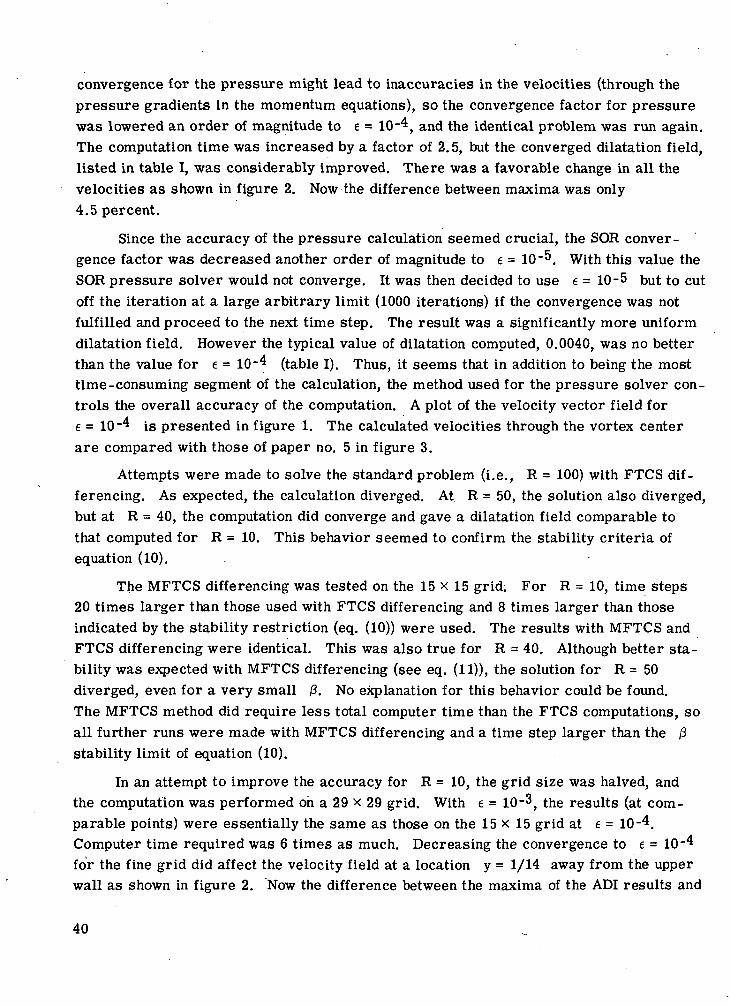
Some simple experiments with the normal gradients used at the boundaries in thepressure solver were performed to see the.effects of different orders of accuracy. Theprevious results were all obtained with a second-order accurate end difference for thegradient; that is,
dp _ 3Pi,l -4Pj,2 + Pi,3 _2 Ay
= 0
A first-order accurate difference at the wall is
9pay
= 0
which was inserted into the SOR routine, and all the previous runs were repeated. Nosubstantial changes due to this new boundary condition were noticed. The velocitiesseemed higher in some instances, but in others the dilatation field seemed a bit lower.
CONCLUDING REMARKS
The Simplified Marker-and-Cell method using primitive variables did not giveaccurate results for flow in the driven cavity because of the inability of the pressure sol-ver to converge to small tolerances. Perhaps, instead of correcting the velocity vectoronly once at each time step, additional pressure corrections could be made until the dila-tation is reduced to a small level. Then a new time step could be calculated. This mightalso produce a more consistent scheme.
Modified forward time and centered space differencing seems to relax the stabilityrestriction on the time step but still retains a limit on cell Reynolds number. The lowerorder boundary condition on the pressure gave marginal improvement in the dilatation,but the computed values of velocity were slightly higher.
41
REFERENCES
1. Roache, Patrick J.: Computational Fluid Dynamics. Hermosa Publ., c.1972.
2. Amsden, Anthony A.; and Harlow, Francis H.: The SMAC Method: A NumericalTechniques for Calculating Incompressible Fluid Flows. LA-4370, Los AlamosSci. Lab., Univ. of California, Feb. 17, 1970.
3. Rubin, S. G.; and Lin, T. C.: Numerical Methods for Two- and Three-DimensionalViscous Flow Problems: Application to Hypersonic Leading Edge Equations.AFOSR-TR-71-0778, U.S. Air Force, Apr. 1971. (Available from DDC asAD 726 547.)
4. Mills, Ronald D.: Numerical Solutions of the Viscous Flow Equations for a Class ofClosed Flows. J. Roy. Aeronaut. Soc., vol. 69, no. 658, Oct. 1965, pp. 714-718;Correction, vol. 69, no. 660, Dec. 1965, p. 880.
42
oinoIIVU
iitfsPMCOOftECOT
wS8§5hH
WHH
T3 eT
§ r
§• .OJo csTo
IH
IIS"
II
s so
ca S
T3 T
!
bfl
T30)
H
5
rt
I
:
O
CO
<1)3 <
M
rt II
u
ort
*J
in IT
in in ^j r-
co c, cj
>a- NC
co c.'O
C
' O
O
O
C>
O
—« -<
—
« -*
—I 0
0o o
o C
' r o o
o o
o c
c- o
C
00
0
O C
; O C
_ C
. O C
O
C'
O
O
O
c"'
CD
O
O
C
. •-* r-« .-<
•—i
or*
O O
O O
O
O O
O C
J O
C
O «
"'o c
• o o
o o
o c
. o o
cj o
o
C C
C
<
O
O
O
f.
—I -I
^ —
I co
o
C
o
c r.i o
c>
<
"i o cj C
' '.•c
c <_• c
C' o
c c
«.' c > e o
t
L' U
"; u" >*i o
r-- O
'~
t' • c\j ^
>o C' r*"
C. 1
<.
C
C • C
: f
'• '~'
»—•
r~*
•-* *~
* *-' CT
'"] C
- C
J '" J
C
C
J C
O
C
' O
C
C
'' * -
cj c
c c
c
<•=' c r
o
ci c
o
« •
cc r^
ff- T
~>
C* f't
^-' rl
«^" «JJ CT
1 •—* C
TO
'
C: I
O •-• -H
.-H
•-!•-< .-I fM
<
•.'•
O
O O
C
J O
O
O
C
O
C
C
• O —
<O
C
C
C
C
' T
' O
C
' O
C
i O
C
f
,-j*—
'^^
*-*
f^jn
^^
cr>
f.~iM
^f^
i
o r
o r. c
i c o
o • j
c: c
j r •-<
C,' O
O r
<_i r-i c.' C
' f. O
C o
C
<dm
in
o so N
- or. c~ <->
<\j >!• -o o', CT
C
t-ii-ii-ii-ip-<
>-<>
^rM
r\irjiv:rM
(r\°
ri »• C
C
O r
Ci f
C C
C'
C'
._. -
. C
J c'
O M
C. i.-i O
Ci 1..- o
C.
ctf135
(
O O
O
O
C
j r ' C.)
CJ C
" C
O C
' —
"o c
o c
o o
o c
> o
o o
o o
CO 'X'
CO
CO
C?' O
•-<
r*"l >^
^O C
O O
^ *f
o r.i o
o o
o c: o
o c
i o r- •-<
C' <_• o
ca
<
.' o o
o o
o o
o
L~\ L
P
U"
1. \O
^*
CJ
G*' '_
.' ^-'
*^ s^
-O
P1 J
O I •
O
' ! O n
o
O
C' O
C' O
-i
O O
O
r * O
O
O
O
O
C
' C) O
O
fi r-! f-
XT in o
r^- 33 a> c' —
i <M co
O
O
O
« '• O
«. • O
O
C
' O
O
C
• rs;
O
r O
C
! O
C.- C
.' O O
C
.« O
C
> I-:
•TI tn in
in 'j^ in. in
in IA
in m
IT
- r.?(.-• '
O
<. • C
i. i C'
f C
' c '.>
'..' n;
o i • c. c.i <•.') c i C
' i i o ' ^ o
< r. 1
lOU
'-in
m^
m -r x
T^
'J'r
^r^
cj
INJ r*J f\j fvj rg f\j
<\j fsj m
r\j r\j r-j -J"
'3 '_
j f r~
c 'V
> o
c
c i c
cj c
- o
43
-e> & fr- -E> & 1—E>
£> 1>
f f f /t t t tf 1 \ \t V \ \
A. ^ *? fc,T \ \ \
A fc > V < '1
-* 1>-
'J- 4-
V f «? ^ <i -5 &
1 4
I I/ /' /
/ / i
/ / -/
fc- O ^
> >
£- > ^
Figure 1.- Computed velocity vectors inside cavity. 15 x 15 grid; R = 10; e = 10~4.
44
nio
c
-o -a
3 C
T>
O L
T)
•)-> S
-3 O
)
O C
Tl
to 00
<_> X
El C
Ti
c
-o -o
-U
S-
3 C
O
SI L
OO
il—
Q
O
IIK•8o£0)sSSPIsS
SO)
O
x
II>>
-ucri
3uo•3CM
45
-0.2 0 0.2 0.4 0.6
I 1 1 1 1 1 1 1 1
u, SMAC solution29 x 29 grid
0 v, SMAC solution29 x 29 grid
Figure 3.- Velocities through closest grid point to vortex centerfor SMAC and ADI methods.
46
5. SOLUTION OF THE INCOMPRESSIBLE DRIVEN CAVITY PROBLEM
BY THE ALTERNATING-DIRECTION IMPLICIT METHOD
Dana J. MorrisLangley Research Center
SUMMARY
A second-order accurate alternating-direction implicit (ADI) method has been usedto solve the two-dimensional incompressible Navier-Stokes equations for flow in a squaredriven cavity. Calculations were made at a Reynolds number of 100 with equally spaced15 X 15, 17 x 17, 33 x 33, and 57 x 57 grids and at a Reynolds number of 10 with a15 x 15 grid. The ADI results agreed well with other solutions. Choosing a criterionfor convergence which was too strict was found to result in no steady-state solution beingreached. A study of the maximum allowable time step for a Reynolds number of 100indicated that time steps many times larger than those used for most consistent explicitmethods could be used for the ADI method.
INTRODUCTION
A second-order accurate efficient implicit method is used to solve the two-dimensional incompressible Navier-Stokes equations for flow in a square driven cavity.(See paper no. 1 by Rubin and Harris for details of the driven cavity problem.) Thisproblem was previously solved by Mills (ref. 1) using an explicit method.
Alternating-direction implicit (ADI) methods were introduced by Peaceman andRachford (ref. 2) and take advantage of a splitting of the time step for multidimensionalproblems to obtain an implicit method which requires only the inversion of a tridiagonalmatrix. The expected unconditional stability of the method allowed larger time stepsthan explicit methods without the complexity of a full matrix reduction routine requiredby one-step implicit methods.
SYMBOLS
K constant
AZ = Ax = Ay
N number of grid points in one direction
47
R Reynolds number
At time step
u axial velocity component
v normal velocity component
x,y axial and normal coordinate, respectively
Ax,Ay spatial increments in x- and y-directions
£ vorticity
v kinematic viscosity
4> stream function
Superscripts:
n index of time step
* intermediate time level
Subscripts:
i,j index of grid point in x- and y-direction, respectively
t differentiation with respect to time
w value at wall
x,y differentiation with respect to x or y
METHOD OF SOLUTION
The nondimensional equations for viscous incompressible two-dimensional flow invorticity—stream-function form which describe the flow field under investigation are
^ = -U?x - V?y + y^ + Kyy (D
48
v ty=£ (2)
and u = i/'y, v = -i//x, and v = 1/R.
Applied to the vorticity transport equation (eq. (1)), the Peaceman-Rachford (ref. 2)alternating -direction implicit (ADI) method advances one time level in the following twosteps.
Step 1
At/2Step 2
f ny
At/2 x y yy
The value £* has no physical meaning.
The method applied to the linear equation has a formal error of order
t o p 2!(At) ,(Ax) ,(Ay) . It is unconditionally stable and consistent. The full second-orderaccuracy of the method can be deteriorated by the nonlinear terms which should be eval-uated as u* and vn for step 1 and as u* and vn+1 for step 2. If the old values
un and vn are used, the formal error is o|At,(Ax) , (Ay) J. Briley (ref. 3) calculated
un and vn and, from the previous values un~^ and vn , linearly extrapolated for-ward to u* and v*. This procedure is stable and appeared second-order accurate;however, additional storage is required for i//n~l. Another procedure (refs. 4 and 5) isto iterate on the entire time step, either to convergence or for a predictor -correctormethod. In either case the error is o|(At)2| and additional storage is required fori//n . It is also possible to calculate «//* after step 1 and to use u* and v* instep 2. Aziz and Heliums (ref. 5) examined these alternatives and found iteration on thefull two steps to be the most accurate. The iteration required to obtain full second-orderaccuracy of the nonlinear terms may not be undesirable since some iteration is anadvantage in achieving accurate boundary values for £.
Although a linear Von Neumann analysis shows the ADI procedure to be uncondition-ally stable, a survey of the literature indicates that the procedure may not be uncondition-ally stable for flows with high Reynolds numbers because of the At time lag of £w- (Seeref. 6.) The degree of convergence for £w to obtain stability is problem dependent.For large At, convergence may be prohibited by nonlinear effects. Also, the program -
49

ing involved with complex boundaries effectively restricts the use of this method to rec-tangular regions.
The tridiagonal nature of the matrix to be solved, although much simpler than thatin fully implicit one-step methods, requires diagonal dominance if error buildup is to beavoided in the matrix inversion. This is equivalent to imposing a restriction on cellReynolds number.
In the present study, the ADI procedure was applied to the vorticity transport equa-tion. Central differencing was used with equal mesh spacing and nonlinear terms werelagged a full time step. After completing a full time step calculation on vorticity, thestream-function equation was solved by a successive overrelaxation (SOR) routine andthe boundary conditions were updated. (The SOR routine was identical with the one usedin the previous paper by Hirsh (paper no. 4).) The vorticity was then calculated for anew time step, rather than being iterated at each time level to achieve a solution whichwas second-order accurate in time, since the interest in this study was in the steady-state solution.
BOUNDARY CONDITIONS
The no-slip condition requires that both u and v (the normal and tangentialgradients of i^) are zero at the stationary walls whereas at .the moving wall u is unity.These conditions are treated by taking a row of image points at a distance AZ = Ax = Ayoutside the boundaries. These values can be related to the interior points by takingderivatives at the boundaries. Thus, the boundary conditions for £ are:
on the stationary walls,
f - ^interior
at the moving wall,
: + ^interior)
The boundary value of i// is zero on all boundaries. Initial conditions are zero every-where except on the moving wall.
50
RESULTS
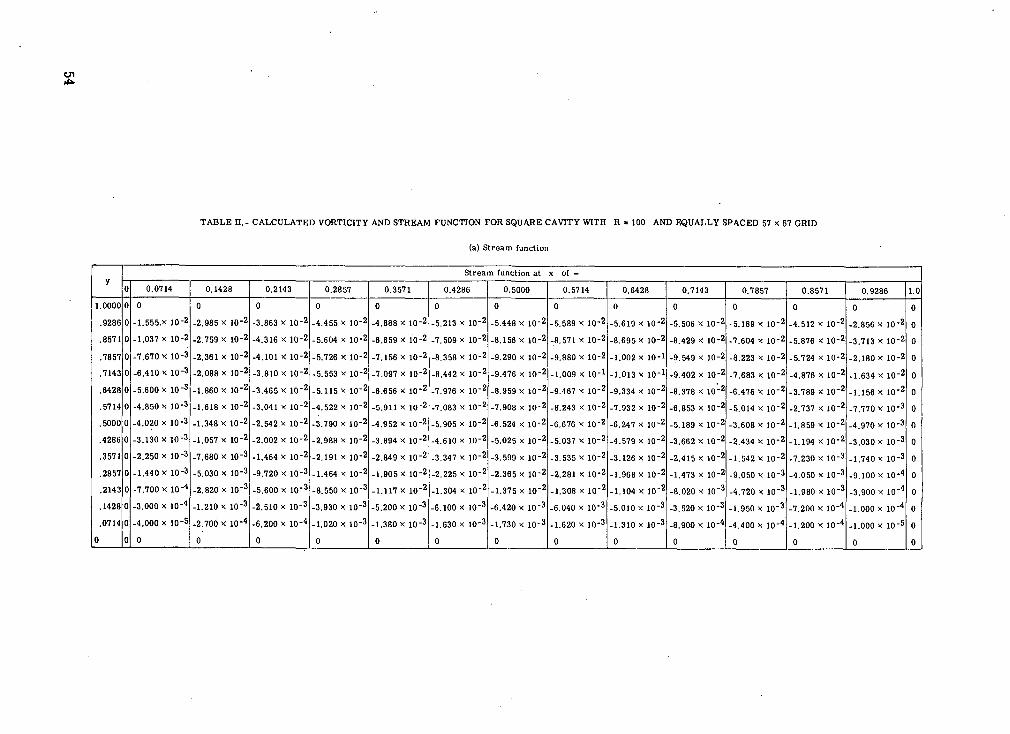
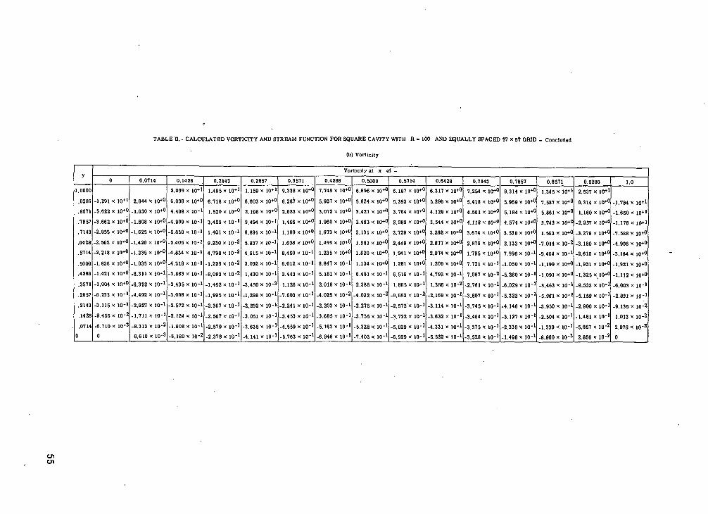
These calculations were made at a Reynolds number of 100 for a square N x Ncavity for N = 15, 17, 33, and 57 and at a Reynolds number of 10 for N = 15. ForN = 17, the problem was also computed with the conservation form of the equations andthe values were found to be much more accurate, although the computer time to achievea converged solution was approximately 2 times longer. As shown in table I, the maxi-mum value of the stream function increases with the number of grid points toward thevalue 0.101 published by Burggraf (ref. 7). The vorticity ? at the midpoint of the mov-ing wall is also shown. For N = 15, the solution was identical with the one published byMills (ref. 1) with a maximum stream function of 0.08742. Machine plots of the velocityvectors and the streamlines of this flow field are shown in figure 1. The calculatedvalues of vorticity £ and stream function ^ for N = 57 are presented in table II.In figure 2 the axial component of velocity u is depicted along a vertical line passingthrough the vortex center, and the calculated values are shown in table HI for the threecases, N = 15 and 57 in nondivergence form and N = 17 in divergence form. Attemptsto increase the accuracy of the nonconservation form by increasing the number of nodalpoints resulted in solutions which did not converge because of a convergence criterionwhich was too strict. The percentage difference between time levels n + 1 and n wasused to check convergence. For N = 15 and 17, solutions were achieved with the con-vergence requirement set at 0.00005. For N = 33, this requirement was repeatedlymade less stringent and was set at 0.001 before a converged solution was reached. Solu-tions for N = 57 did not require further weakening of this convergence criterion. Thisstudy was made for a time step At = Ax, the Courant-Friedrichs-Lewy condition forexplicit methods. Decreasing the Reynolds number to 10 for N = 15 also forced theconvergence requirement to be set at 0.001 and the time step to be decreased. Noattempt was made to find the maximum allowable time step for this Reynolds number.For a Reynolds number of 100, however, such a study was made with the nonconservationform of the equations and the results are shown in figure 3. For N = 15, no solutionwould converge for At greater than 7 Ax. An N of 17 required that At be loweredto 5 Ax. Increasing N to 33 with At = 5 Ax resulted in the solution iterating in theSOR routine until the time limit on the computer was reached. Lowering the time step to3 Ax allowed the solution to converge. For N = 57, convergence in the SOR routinerequired that At = Ax. Thus the maximum allowable time step appears to vary not onlyas a function of Ax but also with the number of grid points used.
51
CONCLUSIONS
An alternating-direction implicit (ADI) method has been used to solve the two-dimensional incompressible Navier-Stokes equations for flow in a square driven cavity.The following conclusions may be drawn:
(1) The ADI technique, although not unconditionally stable as a linear Von Neumannanalysis indicates, does allow time steps many times larger than most consistent expli-cit methods.
(2) Choosing a criterion for convergence which is too strict may result in nosteady-state solution being reached.
REFERENCES
1. Mills, Ronald D.: Numerical Solutions of the Viscous Flow Equations for a Class ofClosed Flows. J. Roy. Aeronaut. Soc., vol. 69, no. 658, Oct. 1965, pp. 714-718;Correction, vol. 69, no. 660, Dec. 1965, p. 880.
2. Peaceman, D. W.; and Rachford, H. H., Jr.: The Numerical Solution of Parabolic andElliptic Differential Equations. J. Soc. Ind. & Appl. Math., vol. 3, no. 1, Mar.1955, pp. 28-41.
3. Briley, W. Roger: A Numerical Study of Laminar Separation Bubbles Using theNavier-Stokes Equations. J. Fluid Mech., vol. 47, pt. 4, June 1971, pp. 713-736.
4. Pearson, Carl E.: A Computational Method for Viscous Flow Problems. J. FluidMech. vol. 21, pt. 4, Apr. 1965, pp. 611-622.
5. Aziz, K.; and Heliums, J. D.: Numerical Solution of the Three-Dimensional Equationsof Motion for Laminar Natural Convection. Phys. Fluids, vol. 10, no. 2, Feb. 1967,pp. 314-324.
6. Roache, Patrick J.: Computational Fluid Dynamics. Hermosa Publ., c.1972.
7. Burggraf, Odus R.: Analytical and Numerical Studies of the Structure of Steady Sepa-rated Flows. J. Fluid Mech., vol. 24, pt. 1, Jan. 1966, pp. 113-151.
52
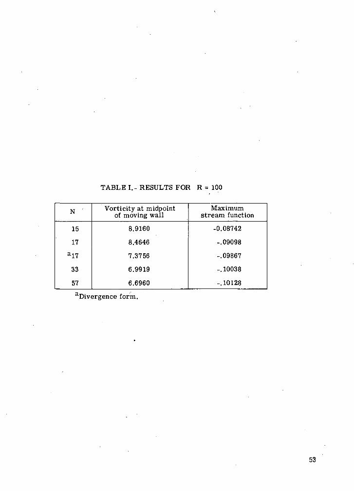
TABLE I.- RESULTS FOR R = 100
N '
15
17
a17
33
57
Vorticity at midpointof moving wall
8.9160
8.4646
7.3756
6.9919
6.6960
Maximumstream function
-0.08742
-.09098
-.09867
-.10038
-.10128
Divergence form.
53
QKODWIQZa -2
§
3
1"oX"rtcotJcFrt
0)
ra
oCDOOCMC»O
r-inCOOc-inCOt-oCOt-OCMSo•<*•
KoinOCOCOCM0COoCOCM
OCO
CM
o"CMOsoo»>
ooooooooooog
oCMoXCDmCO°?CM0XCMin"TCMoXCOmCM0XstnmegoXcnCO"?CMOX§m"?CMOXCOinoXCOCMinoXCOCOCOTegoXmin•<*<
egoXCO§CO
egoXin
CM0Xin"min7oCDCOCM
OegoXCOr-"CMOXCDr-00"?CM0XoCDt-OXenCMCO
egoXenCD°?CMoX£CO
CM0XCO
egoXenomt-
CMOXOiinCO
CMOXsmegoXCD
CO
TCMOXent-
CM0Xc-coO7oinCO
OCM0X0COcvCMOXt-U. J
CMOXCOCMCM
CO
CMOXensen-
oXCMOO7CMOXoCOCOcn
CM0Xscn
CM0XsCOCO
CMOX8LTCMOXsin
CM0Xo*!CMOXCDCO
COoXOt-co17oc-COt-
oCMOXCOCO7CMOXCDCOTCMOXCOCOCOt-
egoXCMOcn0XCO
O7oXcno07
CMOXCDt-cn
eg0XCM•<rCO
CM0Xt-o*7CMOXCOinin
CM0X0COCO
CMOXCOCOo*?oXo*¥oCO
0CM0XCOin7CMoXcnCOr-*vCM0XCOr-CD
* OXCOr-coCO
CMOXCOCO*CMOXt-CD°iCM0XSCO
CMOXCDr-cnc-
CMOXCDinCD
CMoXin"?CMOXinCOCO
CMOXoc§COOXooCOoCOCMs
oCOoX0LTCMoXCOcvCM0XomCMoXCOmCOCD
CMoXCMCOClL7CMoXCOCO
CMOXCO0t-
cgoXCOCOoc-
egoXc»U. J
CMOXCMegT0XoCO
CMOXCOCO
CO0XsCOTos
O 0 O 0 O O
CO CO
CO
-"T V
«
O O 0 O 0 o
X
X
X
X
X
XO 0 O O 0 o
t- CO TJ- O
O
O
7 *? 7 °i *?
7CM
CM CO
CO CO
q<
0 O O 0 0 O
X
X
X
X
X
Xen
^- o o o o
in en
co in co
oco
— i CM
o cn
eg
7 7 T 7 7
CM CM
eg co
co co
O 0 0 O 0 0
X
X
X X X X
CO ^- CM O
O
Oo
co •* m
CM m
CD •*
tn o
c- o>
co CM
T-t cn
J* ••*
CM CM
CM eg
co co
O O O 0 0 O
X
X
X
X
X
Xcn
CM in co o
oco
CD >-i
t- CM
egH
CD •*
•<*• O
inm
co eg
<-i co
eo
CM CM
CM CM
eg co
o o o o o o
X
X
X
X
X
Xt-
Cft CO
CO
*J*
O•<r
r- CM
CD o
~*eg
in i~*
cn <-i
o
°? 7 *? 7 7 "?
CM CM
CM CM
eg co
O O O O O O
X
X
X
X
X
XCD
t-
in
H co
ot-
co co co o
rrCD
O
m
CM CO O
co m
co eg
«-« CD
CM CM
CM CM
CM CO
O O 0 0 O 0
X
X
X
X
X
X<r
in cn m
in o
CM CM
cn eo
t- CM
CD l"
CO
CM
»H
eo
CM eg
CM CM
eg co
o o o o o o
X
X
X
X
X
Xm o t- m -d* o
S^H TJ- CM O
OCD
CO CM
CO H
m
v
co CM ^H CD
eg eg
CM CM
eg co
o o o o o o
X
X
X
X
X
XCM
^ en m c- o
m
o> rf o
~H o
cn co
co cn
--• CM
"T " °? 7 7 "?
CM eg
CM CM
co co
O O O O O O
X
X X
X X X
SCO
—I ^- O
Oco
cn
co
m
co
CO CM
CM i-l
CO CO
CM CM
CM CO
CO CO
o o o o o o
X
X
X
X
X
XCM
CM ^« O
O
OSO CO CM O <-l
o
^ c— co in
CM CM
^H
C7i m
CM
CM
CM
CO
CO
CO
CO
O 0 O 0 O O
X
X
X
X
X
XCO t- O 0 O 0
•
in co
co CM
1-1CO
O
CD O
CO CM
CO CO CO CO ^
^i
O O O O O O
X
X X
X X X
O O 0 0 O O
CM - co m
^i o
oo
>-» eg ^- f~ o
T " °? 7 "7 *?
O O 0 O O O
O
CD
>-" C-
CO CO
O
co t- m ^ CM
o
CM m
oo 1-1
rfm
^" co
CM eg
—i
oinoXo0o7oXooCM7oXo07'oXooenCO
COoXoCO7COoXsCD7COoXoCO7COoXoCOCO7CO0XoCOCO7CO0XoX§CM*?*«•oX0ol-
inoXO§T0S
Oooo0ooo0o
54
,_)
rl
~*
Q
O
O
O
OO
OO
OO
OO
OO
OO
OX
XX
XX
XX
XX
XX
XX
to in
t>
oo
os
5
eg
^- o
co
e->
2
™c
-t
o*
-«
mo
s-
"o
»«
oc
o^
"o
a>
O
O
O
O
O
O
O
O
S
M
^ «
cj efl~~
ooooooooooooooo
xx
xx
xx
x x
'x
xx
xx
x
oi ~H
C
N
co" co
oi
i-i ••*
eo
«ri
~o—
o—
3—
o—
c5—
S—
o—
o—
po
oo
oo
oo
oX
XX
XX
XX
XX
XX
XX
X
I o-
5S
fi r
111 fT
T^
) ^
.M
^H
^H
-H
^M
^H
'"
"
XX
X
XX
X
X
X
X
X
X
XX
X
o
"o
o
o" o
o
o
^
CM
+
+
+
+
-*•
+
+"
Iy
pp
po
pp
oo
pp
po
pp
p
i , x
3 "'
^oooooooooppppo
xx
xx
xx
xx
xx
xx
xx
„
** t
<8
J J J " " "
_p
pp
po
pp
pp
pp
pp
p
" J
^X
XX
XX
XX
XX
ao
di
>• *
I |
po
oc
?o
?o
o7
oo
oo
oo
oo
po
po
pp
<
S
*-
®x
xx
xx
xx
xx
w
t5
°
«
in
• -,
-H
ca
O
£
o
o
o
o
o
o
^
o
S -H
«
>
po
oo
oo
oo
oo
bo
oo
px
xx
xx
xx
x
p I
I'- "
"' -
-' -' -'
- •"' ~
1' «? 1 "? «?
U
o
o
o
o
_
_5
oo
po
oo
oo
pb
op
pp
p
xx
xx
xx
xx
-^ o>
to
N
**
^H
«
co
co
«•>
*^
t—
w
in
^
m
+
+
+Q
O
OO
OO
OO
OO
OO
OO
OO
3
Jg
xx
xx
xx
xx
xEH
o
^i io
_ o
ob
oo
oo
oo
oo
pp
Q
2x
xx
xx
y>
rx
x
U
pu
in
ec
p%
O«
oe
po
>«
Nt
nt
-r
-O
>o
oH
~
*5 —
" (o
« eo"
—"
c» V
r*
°? r 1
r 1 *^
^ *?" **?
Du3 .
O
f^
Jx
xx
xx
xx
xx
xx
xx
xx
•O
>O
>O
O«
O«
-*
CO
MO
t-
J<I
oooooooobbbooo
H
V
^-
-H
,-
,_
««
^-
<-
H_
.-
.«
.*
.-
t
^
xx
xx
xx
xx
xx
xx
xx
!«, =
«,»
«, =
„„,
eg
-H
ri' '
' -'
^
co
eo
V
ci
«"
~^-
o
^o
o
o
o"
o
oo
oo
oo
oo
op
pp
oo
XX
XX
XX
XX
7
"?
*7'
*?
°?
oo
co
55
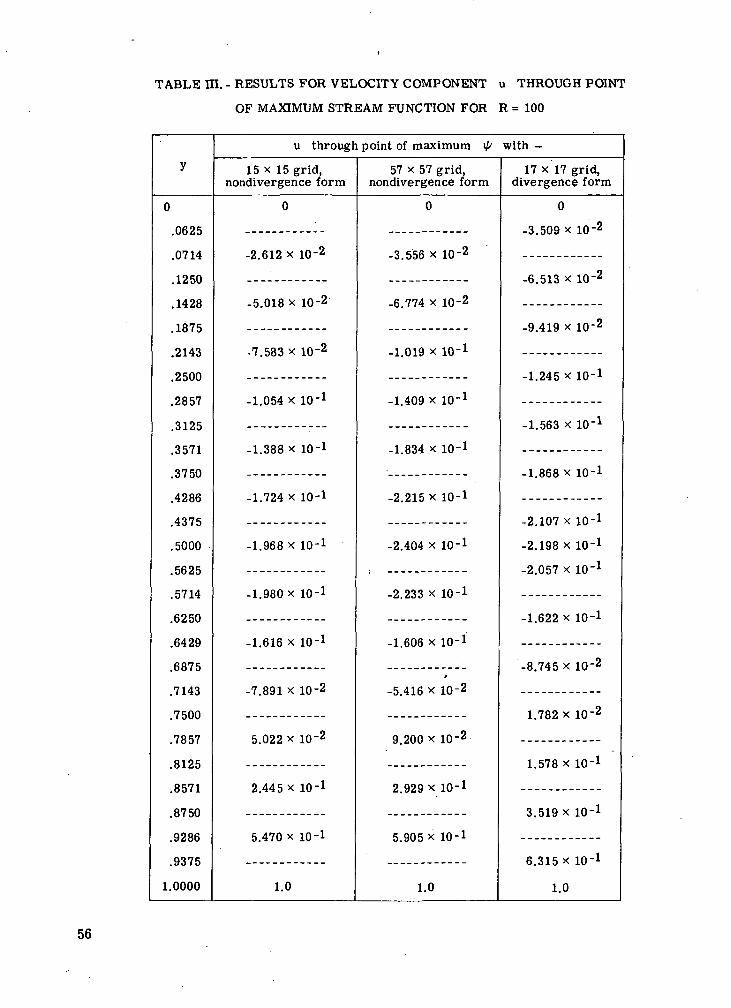
TABLE HI. - RESULTS FOR VELOCITY COMPONENT u THROUGH POINT
OF MAXIMUM STREAM FUNCTION FOR R = 100
y
0
.0625
.0714
.1250
.1428
.1875
.2143
.2500
.2857
.3125
.3571
.3750
.4286
.4375
.5000
.5625
.5714
.6250
.6429
.6875
.7143
.7500
.7857
.8125
.8571
.8750
.9286
.9375
1.0000
u through point of maximum i// with —
15 x 15 grid,nondivergence form
0
-2.612 x ID"2
-5.018 x 10⁻²
-7.583 x ID'2
-1.054X lO"1
-1.388X 10⁻¹
-1.724 x 10⁻¹
-1. 968X10- 1
-1.980X 10⁻¹
-1.616 X 10⁻¹
-7.891 x lO-2
5.022 x lO-2
2.445 x 10⁻¹
5.470 x 10⁻¹
1.0
57 x 57 grid,nondivergence form
0
-3.556 x ID'2
-6.774 x 10⁻²
-1.019 x lO-1
-1.409 x 10⁻¹
-1.834 x 10⁻¹
-2.215 x 10⁻¹
-2.404 x 10⁻¹
-2.233 x 10⁻¹
-1.606 x 10⁻¹
t
-5.416 x lO-2
9.200 x ID"2
2.929 x 10⁻¹
5.905 X 10⁻¹
1.0
17 x 17 grid,divergence form
0
-3.509 x lO-2
-6.513 x lO-2
-9.419 x lO-2
-1.245X 10⁻¹
-1.563 x lO"1
-1.868 x 10⁻¹
-2.107 x 10⁻¹
-2.198 x 10⁻¹
-2.057 x 10'1
-1.622 x 10⁻¹
-8.745 x ID"2
1.782 x lO-2
1.578X ID"1
3.519X 10⁻¹
6.315X 10⁻¹
1.0
56
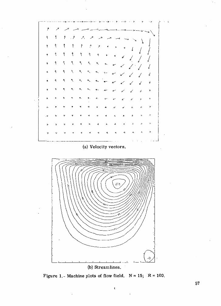
t f . t /; x» >
t t f f ;a ,«
/x .'
/
* v- v~
"• «- •»- «- ir t P
> ^ V • ? ^ - 4 4 l 4 f i & ^
(a) Velocity vectors.
(b) Streamlines.
Figure 1.- Machine plots of flow field. N = 15; R = 100.
57
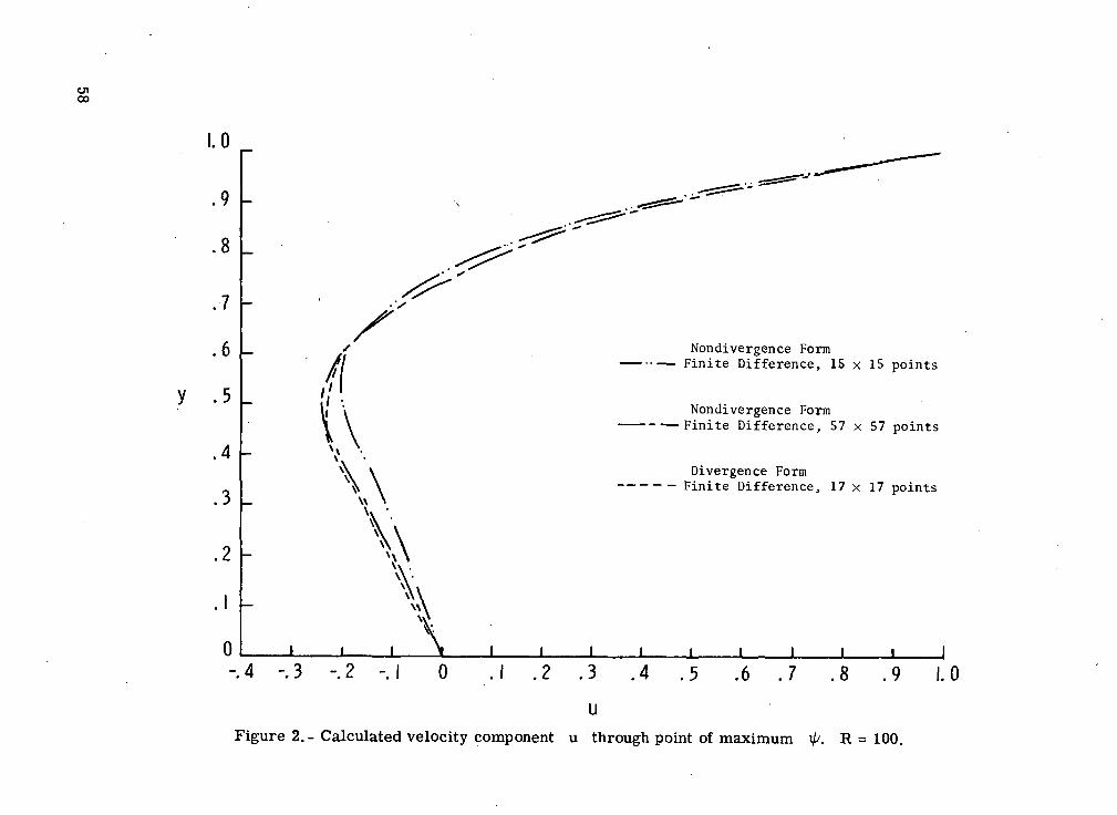
Oo0)
gI-ooooT30)3O*-rt
0<M
58
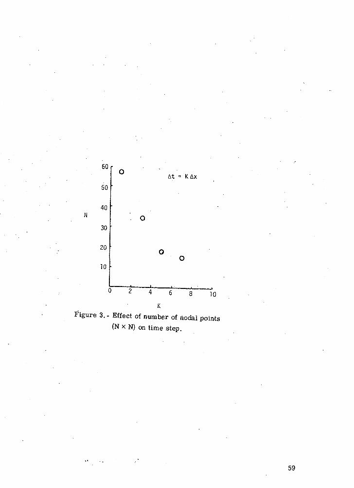
K
Figure 3- - Effect of number of nodal points
(N * N) on time step.

Page intentionally left blank
6. COMPARATIVE STUDY OF TWO NUMERICAL TECHNIQUES FOR
THE SOLUTION OF VISCOUS FLOW IN A DRIVEN CAVITY
Robert E. Smith, Jr., and Amy Kidd*Langley Research Center
SUMMARY
Numerical solutions have been obtained for the steady two-dimensional flow of aviscous incompressible fluid in a rectangular cavity. The Reynolds number has beenvaried from 100 to 5000. The conservative stream-function—vorticity form of the two-dimensional incompressible Navier-Stokes equations was solved. Two techniques(alternating-direction implicit and hopscotch) have been applied to the vorticity equation.The stream-function equation has been solved by successive over relaxation and by theBuneman direct method. The investigation assesses which combination of these tech-niques, applied to the stream-function—vorticity form of the Navier-Stokes equations, isthe most computationally efficient. Width-depth ratios of 1, 2, and 4 have been used inthis numerical experiment. Relative efficiency has been based on the central processingtime of each technique run on the same computer. The results indicate that thealternating-direction implicit technique for solving the vorticity equation and theBuneman direct method for solving the stream-function equation yield the most efficientcombination of the techniques studied. In addition, solutions have been obtained atReynolds numbers of 100, 1000, and 5000 with a second-order accurate approximation.
INTRODUCTION
Numerical solutions of the stream-function—vorticity form of the Navier-Stokesequations describing two-dimensional flow have been the subject of many investigations.In particular, the flow .properties of a viscous incompressible fluid within a rectangularcavity whose upper surface is translating with uniform velocity have been established forlow Reynolds numbers. (See paper no. 1 by Rubin and Harris.) This study has attemptedto increase understanding of optimum solution techniques for solving the two-dimensionalNavier-Stokes equations at low Reynolds numbers. The optimum solution technique istaken to be the one which provides a steady-state solution in minimum computer timewith the least complex program. It is recognized that optimum in this sense is computerdependent. However, the results should hold for any third generation computer. Twotechniques which appear to be near optimum for solving the vorticity equation are thealternating-direction implicit (ADI) and hopscotch (HS) procedures. Reference 1 shouldbe referred to for the ADI technique and reference 2 is adequate for the HS technique.
*Computer Sciences Corporation, Hampton, Va.
61
For solving the stream-function equation the successive overrelaxation (SOR) techniqueand the Buneman direct method (BDM) are candidates for being optimum solution proce-dures. Reference 3 should be consulted for the BDM and reference 2 is adequate for theSOR technique.
The two-dimensional Navier-Stokes equations have been described in conservationform and approximate boundary conditions established. A computer program with theoption of using the ADI or HS technique for the solution of the vorticity equation has beenwritten. In addition, the HS technique is applied in two ways. The first approach (HS1)is direct application of the difference equations at the even and odd grid points. Thesecond approach (HS2) is application of a combined difference equation when the iterationplus the grid point is even. The second approach should reduce the number of operationsby approximately 40 percent. The computer program has the option of solving thestream-function equation by either SOR or BDM. The BDM subroutine used in the com-puter program is one written by Buzbee. (See ref. 3.) The Buneman algorithm is muchmore complex than the SOR algorithm; however, once the algorithm is written into acomputer program, it is easily applied. Note that if the domain of interest is not rec-tangular, the Buzbee routine and the BDM are not directly applicable. The computerprogram has been written with the ability to vary time step, grid size, Reynolds number,and initial conditions. With this program as an experimental tool, many runs varyingtime step, grid size, Reynolds number, and width-depth ratio with each of the combina-tion techniques - ADI-SOR, ADI-BDM, HSl-SpR, HS1-BDM, HS2-SOR, and HS2-BDM -have been made on a CDC 6400 computer and appropriate statistics recorded.
SYMBOLS
N,M dimensions of grid (see fig. 1)
R Reynolds number
t time
At time step
U uniform velocity at upper surface (see fig. 1)
u axial velocity
- -v normal velocity
62
x,y axial and normal coordinate, respectively
Ax,Ay spatial increments in x- and y-directions
0 = Ax/Ay
£ vorticity
4> stream function
a; convergence parameter in SOR approximation
Superscripts:
k index of iteration
n index of time step
Subscripts:
i,j index of grid point in x- and y-direction, respectively
in grid point inside surface
out grid point outside surface
s grid point on surface
t differentiation with respect to t
x,y differentiation with respect to x or y
Abbreviations:
ADI alternating direction implicit
BDM Buneman direct method
HS1 hopscotch method 1
63
HS2 hopscotch method 2
SOR successive overrelaxation
GOVERNING EQUATIONS AND BOUNDARY CONDITIONS
The normalized stream -function — vorticity conservation form of the two-dimensional incompressible Navier -Stokes equations is:
<D
The boundary conditions on the stream -function equation (eq. (2)) for flow in acavity with the upper surface translating to the left with uniform velocity U = 1 andwith no flow at the other boundaries are (see fig. 1):
at upper surface (moving to left),
<//y = "I ^ = 0 I// = 0
at bottom, left, and right surfaces,
i/'y = 0 i//x = 0- i// = 0
The boundary conditions on the vorticity equation are obtained by central differ-encing equation (2), by applying the boundary conditions for the stream function, and byenforcing reflection at the boundary. They are:
at upper surface,
_
(Ay)2
/ , -out2 Ay
64
or combining these conditions results in
2i//ln - 2 Ay _
(Ay)2 S
at bottom surface,
(Ay)
or
(Ay)2 bS
at left and right surfaces,
or
(Ax)2 S
FINITE-DIFFERENCE APPROXIMATIONS
Because of the complexity of the BDM, an explanation of this method is not given.Details of the method are given by Buzbee, Golub, and Nielson in reference 3.
65
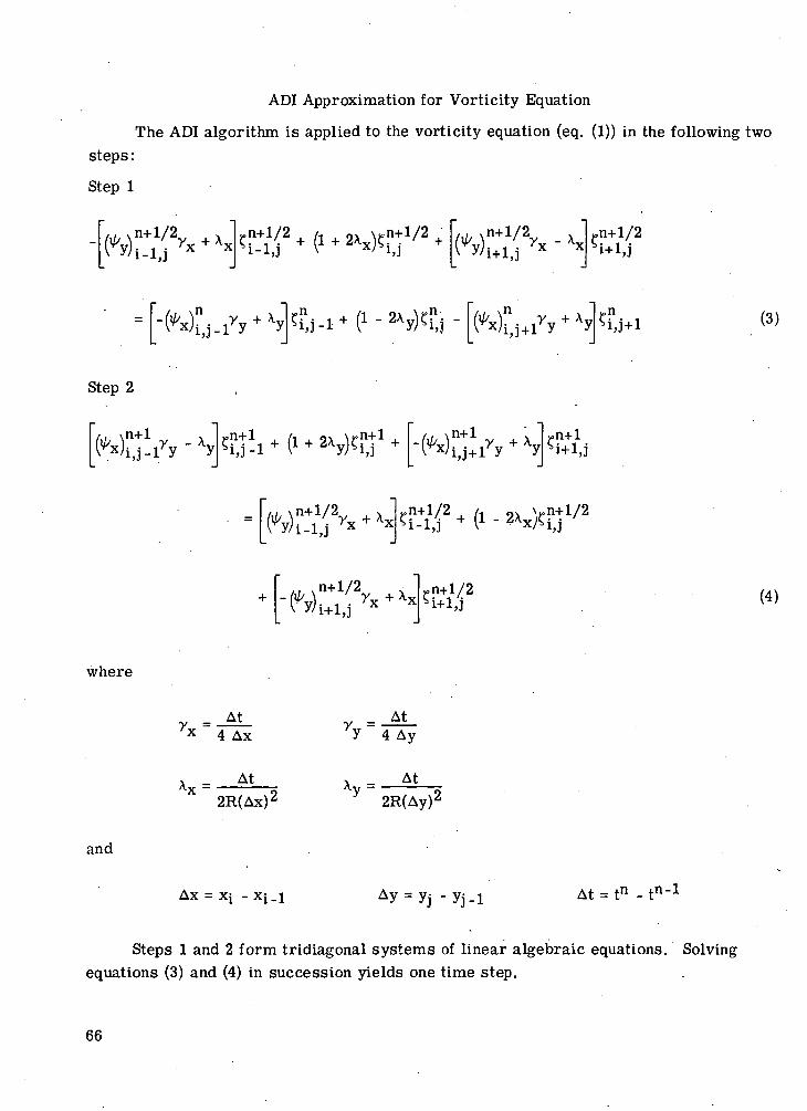
ADI Approximation for Vorticity Equation
The ADI algorithm is applied to the vorticity equation (eq. (1)) in the following twosteps:
Step 1
(3)
Step 2
n+1
n+l/2 l/2
-n+1
(4)
where
and
-At ,, _ At4 Ax
At
'y 4 Ay
\ - At
2R(Ax)2
Ax =
2R(Ay)2
Ay = yi - yi_l At = tn - tn~
Steps 1 and 2 form tridiagonal systems of linear algebraic equations. Solvingequations (3) and (4) in succession yields one time step.
66
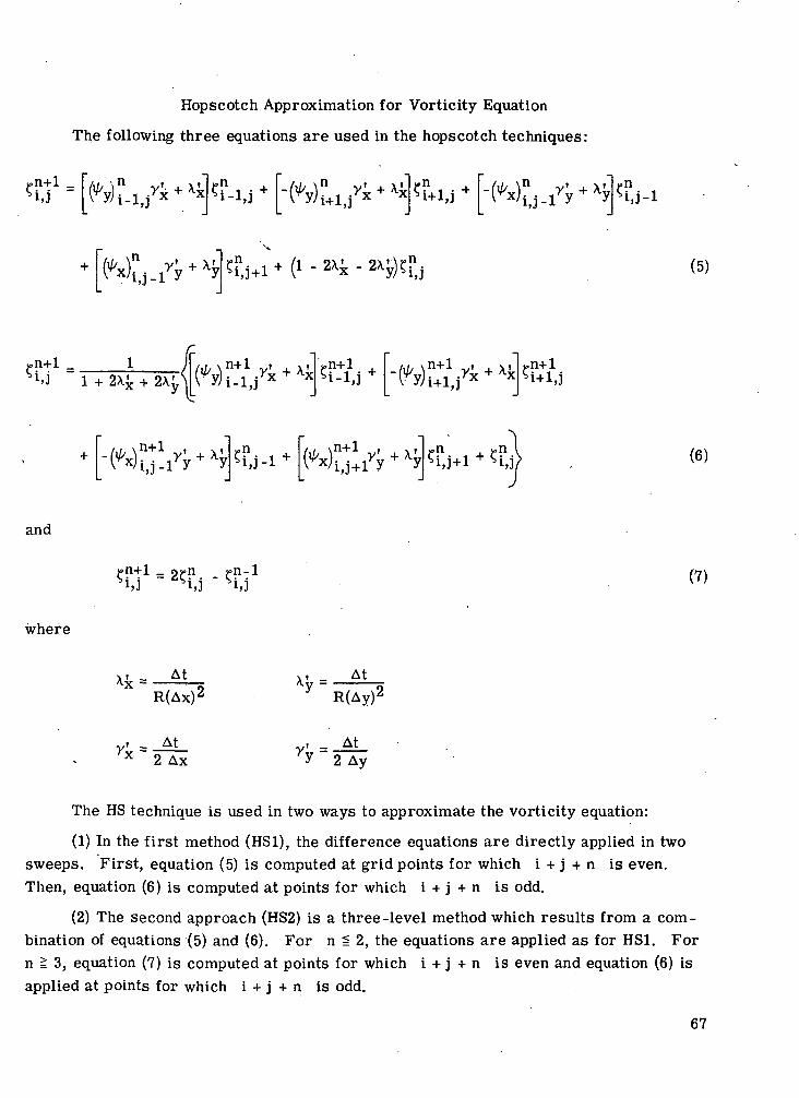
Hopscotch Approximation for Vorticity Equation
The following three equations are used in the hopscotch techniques:
>i, j - l
(5)
. \iy
x i»n+l
n+l
n+1
1+1JJ
, ,(6)
and
where
p+1 _ oi»n rn-1j i ''Sj ^ S; i1>J L>J 1>J
(7)
At
Vv = 2 Ax 2 Ay
The HS technique is used in two ways to approximate the vorticity equation:
(1) In the first method (HS1), the difference equations are directly applied in twosweeps. First, equation (5) is computed at grid points for which i + j + n is even.Then, equation (6) is computed at points for which i + j + n is odd.
(2) The second approach (HS2) is a three-level method which results from a com-bination of equations (5) and (6). For n ^ 2, the equations are applied as for HS1. Forn ^ 3, equation (7) is computed at points for which i + j + n is even and equation (6) isapplied at points for which i + j + n is odd.
67
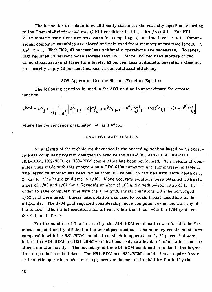
The hopscotch technique is conditionally stable for the vorticity equation accordingto the Courant-Friedrichs-Lewy (CFL) condition; that is, U(At/Ax) ^ 1. For HS1,21 arithmetic operations are necessary for computing £ at time level n + 1. Dimen-sional computer variables are stored and retrieved from memory at two time levels, nand n + 1. With HS2, 43 percent less arithmetic operations are necessary. However,HS2 requires 33 percent more storage than HS1. Since HS2 requires storage of two-dimensional arrays at three time levels, 43 percent less arithmetic operations does notnecessarily imply 43 percent increase in computational efficiency.
SOR Approximation for Stream -Function Equation
The following equation is used in the SOR routine to approximate the streamfunction:
2\L +
where the convergence parameter u> is 1.67351.
ANALYSIS AND RESULTS
An analysis of the techniques discussed in the preceding section based on an exper-imental computer program designed to execute the ADI-SOR, ADI-BDM, HS1-SOR,HS1-BDM, HS2-SOR, or HS2-BDM combination has been performed. The results of computer runs made with this program on a CDC 6400 computer are summarized in table I.The Reynolds number has been varied from 100 to 5000 in cavities with width-depth of 1,2, and 4. The basic grid size is 1/16. More accurate solutions were obtained with gridsizes of 1/32 and 1/64 for a Reynolds number of 100 and a width-depth ratio of 1. Inorder to save computer time with the 1/64 grid, initial conditions with the converged1/32 grid were used-. Linear interpolation was used to obtain initial conditions at themidpoints. The 1/64 grid required considerably more computer resources than any ofthe others. The initial conditions for all runs other than those with the 1/64 grid arei// = 0.1 and 5 = 0.
For the solution of flow in a cavity, the ADI-BDM combination was found to be themost computationally efficient of the techniques studied. The memory requirements arecomparable with the HS1-BDM combination which is approximately 20 percent slower.In both the ADI-BDM and HS1-BDM combinations, only two levels of information must bestored simultaneously. The advantage of the ADI-BDM combination is due to the largertime steps that can be taken. The HS1-BDM and HS2-BDM combinations require fewerarithemetic operations per time step; however, hopscotch is stability limited by the
68
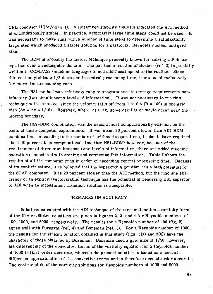
CFL condition (U(At/Ax) = l). A linearized stability analysis indicates the ADI methodis unconditionally stable. In practice, arbitrarily large time steps could not be used. Itwas necessary to make runs with a number of time steps to determine a satisfactorilylarge step which produced a stable solution for a particular Reynolds number and gridsize.
The BDM is probably the fastest technique presently known for solving a Poissonequation over a rectangular domain. The particular routine of Buzbee (ref. 3) is partiallywritten in COMPASS (machine language) to add additional speed to the routine. Sincethis routine yielded a 1/3 decrease in central processing time, it was used exclusivelyfor more time-consuming runs.
The HS1 method was relatively easy to program and its storage requirements sat-isfactory (two simultaneous levels of information). It was not necessary to run thistechnique with At = Ax since the velocity falls off from 1 to 0.6 (R = 100) in one gridstep (Ax = Ay = 1/16). However, when At > Ax, some oscillation would occur near themoving boundary.
The HS2-BDM combination was the second most computationally efficient on thebasis of these computer experiments. It was about 20 percent slower than ADI-BDMcombination. According to the number of arithmetic operations, it should have requiredabout 40 percent less computational time than HS1-BDM; however, because of therequirement of three simultaneous time levels of information, there are added machineoperations associated with storing and retrieving this information. Table I shows theresults of all the computer runs in order of ascending central processing time. Becauseof its explicit nature, it is believed that the hopscotch algorithm has a high potential forthe STAR computer. It is 20 percent slower than the ADI method, but the machine effi-ciency of an explicit (vectorizable) technique has the potential of rendering HS1 superiorto ADI when an inconsistent transient solution is acceptable.
REMARKS ON ACCURACY
Solutions calculated with the ADI technique of the stream-function—vorticity formof the Navier-Stokes equations are given in figures 2, 3, and 4 for Reynolds numbers of100, 1000, and 5000, respectively. The results for a Reynolds number of 100 (fig. 2)agree well with Burggraf (ref. 4) and Bozeman (ref. 5). For a Reynolds number of 1000,the results for the stream function obtained in this study (figs. 3(a) and 3(b)) have thecharacter of those obtained by Bozeman. Bozeman used a grid size of 1/50; however,his differencing of the convective terms of the vorticity equation for a Reynolds numberof 1000 is first-order accurate, whereas the present solution is based on a central-difference approximation of the convective terms and is therefore second-order accurate.The contour plots of the vorticity solutions for Reynolds numbers of 1000 and 5000
69
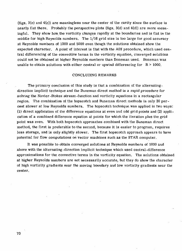
(figs. 3(c) and 4(c)) are meaningless near the center of the cavity since the surface isnearly flat there. Probably the perspective plots (figs. 3(d) and 4(d)) are more mean-ingful. They show how. the vorticity changes rapidly at the boundaries and is flat in themiddle for high Reynolds numbers. The 1/16 grid size is too large for good accuracyat Reynolds numbers of 1000 and 5000 even though the solutions obtained show theexpected character. A point of interest is that with the ADI procedure, which used cen-tral differencing of the convective terms in the vorticity equation, converged solutionscould not be obtained at higher Reynolds numbers than Bozeman used. Bozeman wasunable to obtain solutions with either central or upwind differencing for R > 1000.
CONCLUDING REMARKS
The primary conclusion of this study is that a combination of the alternating -direction implicit technique and the Buneman direct method is a rapid procedure forsolving the Navier-Stokes stream-function and vorticity equations in a rectangularregion. The combination of the hopscotch and Buneman direct methods is only 20 per-cent slower at low Reynolds numbers. The hopscotch technique.was applied in two ways:(1) direct application of the difference equations at even and odd grid points and (2) appli-cation of a combined difference equation at points for which the iteration plus the gridpoint was even. With both hopscotch approaches combined with the Buneman directmethod, the first is preferable to the second, because it is easier to program, requiresless storage, and is only slightly slower. The first hopscotch approach appears to havepotential for flow computations on vector machines such as the STAR computer.
It was possible to obtain converged solutions at Reynolds numbers of 1000 andabove with the alternating-direction implicit technique which used central-differenceapproximations for the convective terms in the vorticity equation. The solutions obtainedat higher Reynolds numbers are not necessarily accurate, but they do show the characterof high vorticity gradients near the moving boundary and low vorticity gradients near thecenter.
70
REFERENCES
1. Peaceman, D. W.; and Rachford, H. H., Jr.: The Numerical Solution of Parabolic andElliptic Differential Equations. J. Soc. Ind. & Appl. Math., vol. 3, no. 1, Mar.1955, pp. 28-41.
2. Roach, Patrick J.: Computational Fluid Dynamics. Hermosa Publ., c.1972.
3. Buzbee, B. L.; Golub, G. H.; and Nielson, C. W.: On Direct Methods for SolvingPoisson's Equations. SIAM J. Numerical Anal., vol. 7, no. 4, Dec. 1970,pp. 627-656.
4; Burggraf, Odus R.: Analytical and Numerical Studies of the Structure of Steady Sep-arated Flows. J. Fluid Mech., vol. 24, pt. 1, Jan. 1966, pp. 113-151.
5. Bozeman, James D.; and Dalton, Charles: Numerical Study of Viscous Flow in aCavity. J. Comput. Phys., vol. 12, no. 3, July 1973, pp. 348-363.
71
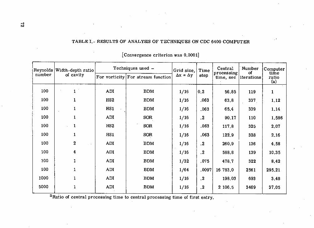
oooocoOPuOT
MIOWEHFHO05WHenWw
oooCOrtCO0)
'Coo0)tf0)oo
"tj C
U O
&a •'5'u
Numberof
iterations
Centralprocessingtime, sec
a> ~
ad
^ <
UH
"£
dT !>
,N <
« .11
*Oiques used -
For stream function
Techn
For vorticity
o1J3 Si
-&>
•o °4- -8§en .S
0o .0
II
coTH
TH
inTH
TH
TH
TH
O5
t~
Oi
CO
TH
co eo
THTH
co
eo TH
in
t-O
O
OO
^
TH
co co
m
o
in
co
co
os
co eo
CO
CD
CM
O
O
CM
t- co
oo
o
TH
in
CM
C
M
Tj<
in
oo
coCM
CM
CO
eo co
TH
oo O
i o>
C-
CM
0
iH
CM
C
OtH
iH
C
M
co eo
CO
CDO
O
C
M
m
CM
TH
oo
o
oo
m
co
TH
O
J
CM
O)
CM
tH
C
OCO
C
M
CD
O
iTH
eo in
coCM
CO
oo c-
o
o00
00
C
O
00OO
£•*
00 O
5in
r}<
t—
TH
coTH
t>m
at
t- o
CM
O
O
CM
inoc-eoO5
CO
COincoorHCM
CM
oCD
C
D
CO
C
O
\ \ ^. ^. CO
CD
CD
\ \ ^
CO
CM
T}<
coco<H
p p
p BPQ
PQ
PQ
01
P
w
ra
P^J
^H
S
H
^<
o
o
o
oo
o
o
oTH
TH
iH
TH
§ § P
OT CO
.CQ
co co
Q
O
O
0o
o
o
P
P
P
PPQ
PQ PQ
PQ
P
P
P
P
Tj<
TH
TH
TH
o
o
o
oo
o
o
o
TH
T
H
TH
OTH
PPQPTH
oooin
time to central processing time of first entry.aRatio of central processing
72
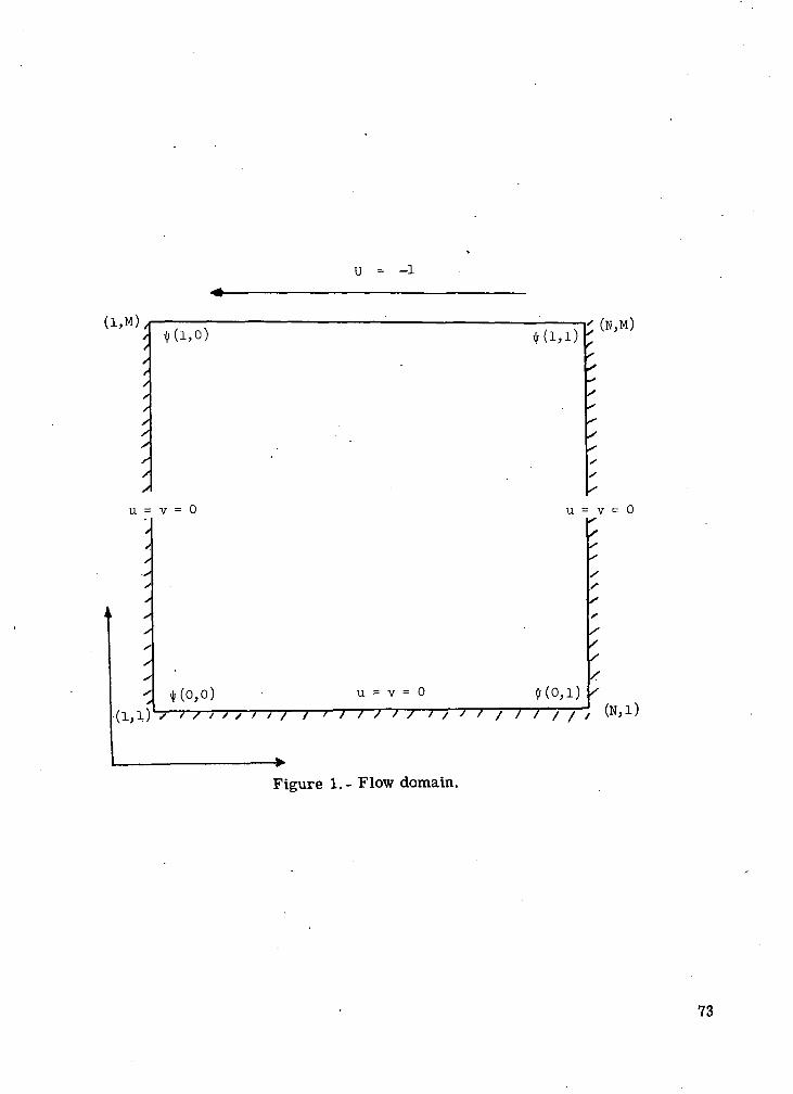
u = -i
(I ,M)X- £ (H,M)
u = v = 0
•(1,1)
s
u = v = 0
/•
t(o,o)/ /< / / > x > i /
u = v = 0
"7 / / / / 7~~7"t(o,i)
/ / / / / /
Figure 1.- Flow domain.
73
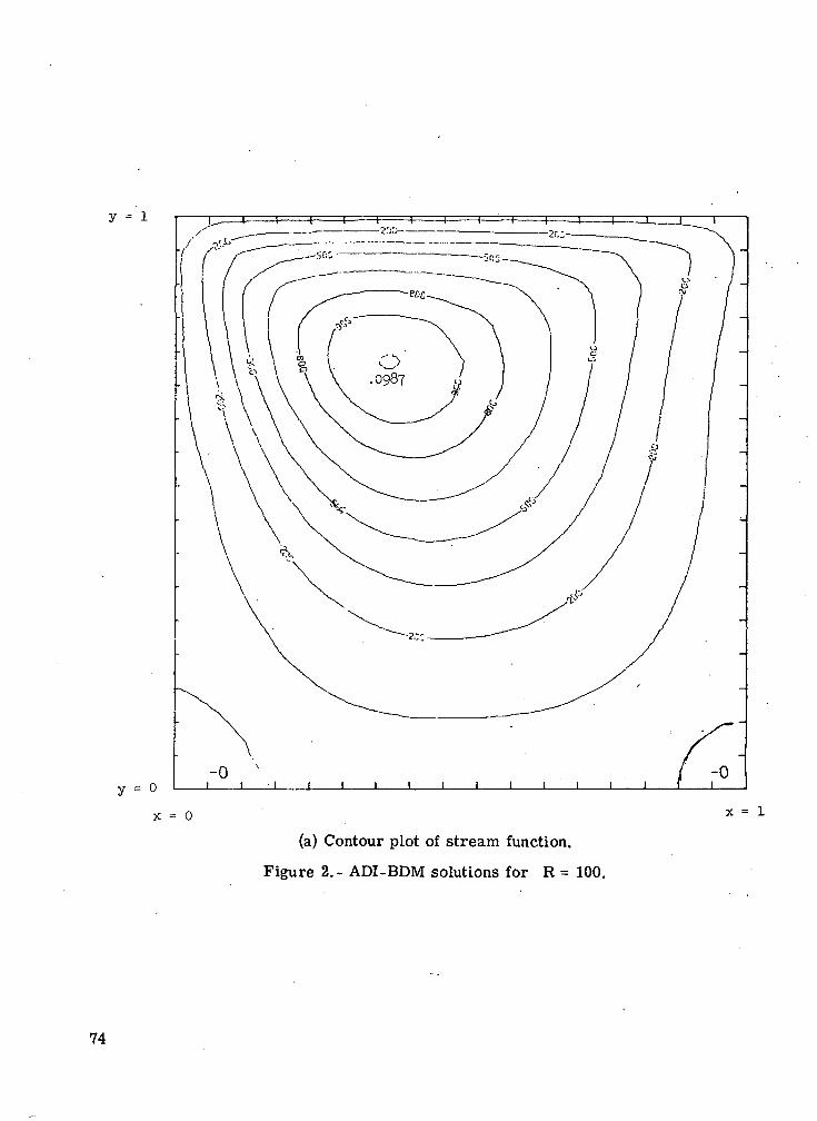
y = i
y = 0
x = 0
(a) Contour plot of stream function.
Figure 2.- ADI-BDM solutions for R = 100.
x = 1
74
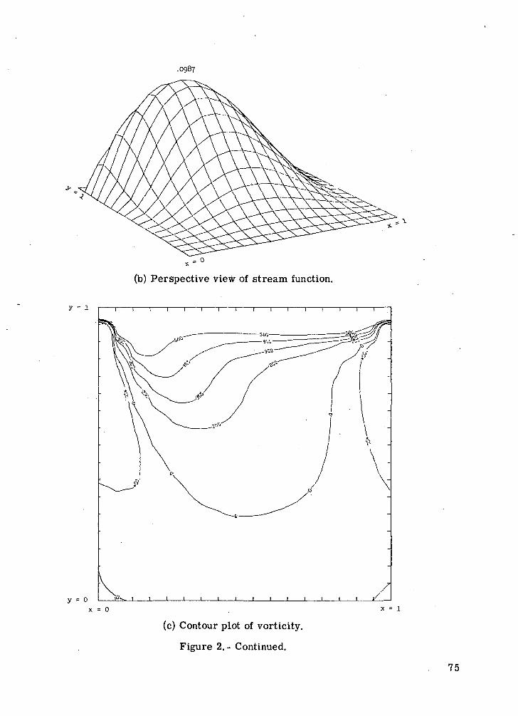
.0987
y = i
y = o
(b) Perspective view of stream function.
x = 0 X = 1
(c) Contour plot of vorticity.
Figure 2. - Continued.
75
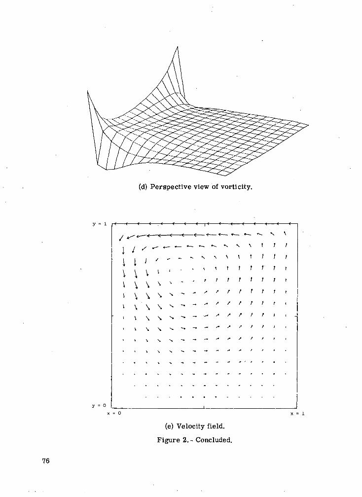
(d) Perspective view of vorticity.
I 1\ \\ Xi X1 \
\ \
-. N \
t f tt / / t
t f f r f it r t t t t/ / t t t i/• t t t t i/ • / / • / i i _ j/• / / / i i
y = ox = 0
76
(e) Velocity field.
Figure 2.- Concluded.
x = 1
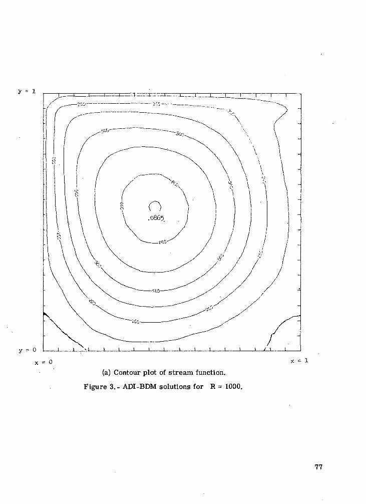
y = i
= 0 I 1 1 v ' 1 — 1 1 1 1 L . . L L I I I / 1
x = 0
(a) Contour plot of stream function.
Figure 3.- ADI-BDM solutions for R = 1000.
= l
77
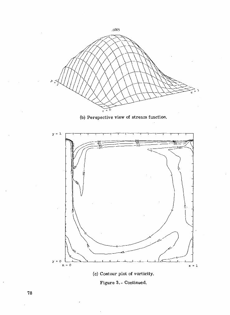
.0865
(b) Perspective view of stream function.
= i
y = ox. = 0
(c) Contour plot of vorticity.
Figure 3.- Continued.
X = 1
78
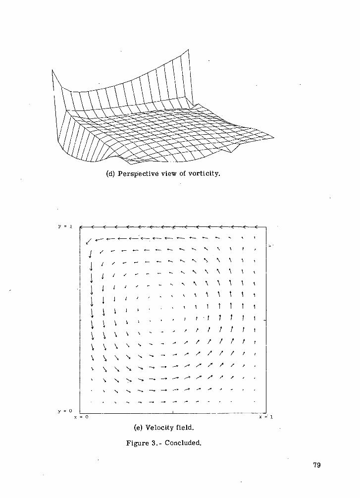
(d) Perspective view of vorticity.
y = i
I ' " "I J ' '\ < ' '\ J ' 'I J J '1 i l '1 i > l
\ \ ^ ^v \ \ ^\ \ \ N-\ \ \ N
y = ox = 0
»^ ^ v \ \ t ,
^ V \ \ \ A i
v N \ \ \ \ x
S \ \ "\ \ \ \
^ \ \ \ \ \ 1
1 1 1 1 1 1 1
/ / •; ? f f i, r t t t 1 \
s s
s* S
(e) Velocity field.
Figure 3.- Concluded.
X =' 1
79
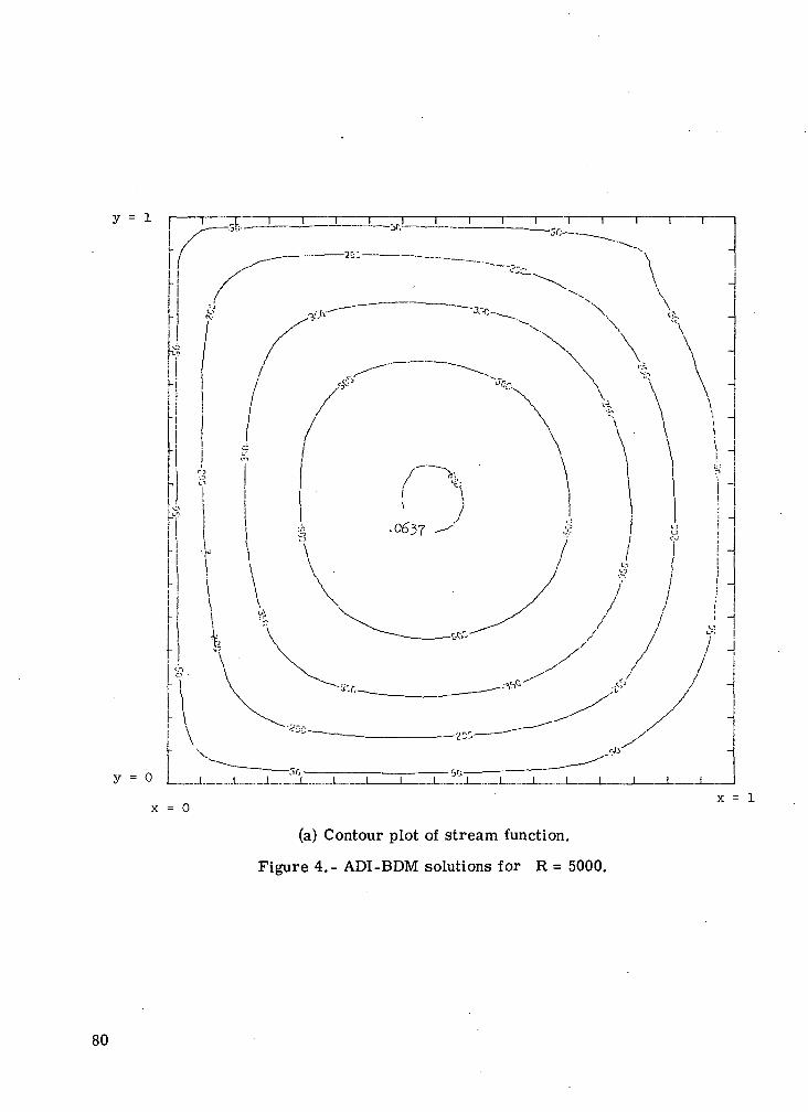
y = i i i T i 1 1 i i i
y = o | I I I I I J I I I I
(a) Contour plot of stream function.
Figure 4.- ADI-BDM solutions for R = 5000.
X = 1
80
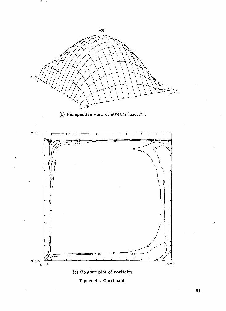
.0637
= \
(b) Perspective view of stream function.
y = i
y .== ox = o
(c) Contour plot of vorticity.
Figure 4.- Continued.
X = 1
81
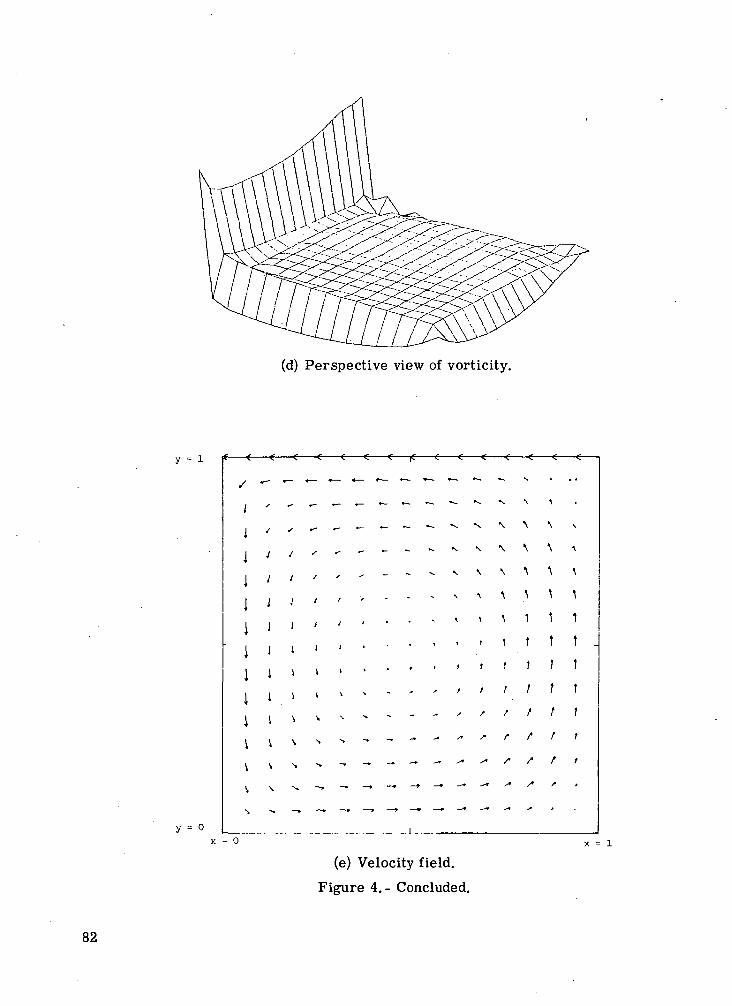
y =
y = 0
•n = 0
(d) Perspective view of vorticity.
\
1Jiiiiii1IVV
N
J '
j J , * • - - - -
\ l < ' ' - - "
J 1 / ' ' - - -
J , t , - • ' -
J 1 1 1 ' ' '
J 1 I ' ' ' ' '
1 J I 1 - - ' '
I \ ^ N - ~ - -
1 \ N ^ - - - "
, „ „ -, , -. - -
\ -~« ~» — — » — • — » — »
- , _ _ _ _ _ _ ^
— ^ ...
•^ -^ V \ \
^ V \ \ \ V
V N \ \ \ \
K \ \ \ \ \
N \ \ ^ \ ^. t ^ 1 1 1
* t 1 t 1 t
• r i t t t
/ / / t f t
, , / f r i* s f f t r
^ ^ /• /• / /
- ^ " ^ ' '
(e) Velocity field.
Figure 4. - Concluded.
82
7. CALCULATION OF STEADY VISCOUS FLOW IN A SQUARE DRIVEN
CAVITY BY THE ARTIFICIAL COMPRESSIBILITY METHOD
John T. SuttlesLangley Research Center
SUMMARY
Numerical solutions of steady viscous flow in a two-dimensional cavity have beenobtained by the method of artificial compressibility. The method, originally presentedby A. J. Chorin, was programed for a computer solution and checked against a simplechannel flow problem which has an analytical solution. The comparison indicated thatthe method was correctly programed. Results for a square cavity at a Reynolds num -ber of 100 were then obtained and compared with published results. This comparisonshowed that the method produces good results for velocities but that the computed pres-sures are unreliable.
INTRODUCTION
The literature, in recent years, includes numerous studies of different numericalmethods for obtaining finite-difference computer solutions to fluid mechanics problems.(See ref. 1, for examples.) Consequently, a study was undertaken to compare the abilityof several reported methods to compute the motions of a viscous incompressible fluid ina two-dimensional square cavity which has one of its walls undergoing uniform transla-tion. (See paper no. 1 by Rubin and Harris.) This problem was selected because it rep-resents a simple example of a steady flow involving closed streamlines and it has beenstudied extensively in the literature. (See refs. 2 to 6.) The present paper is one of aseries of papers dealing with this problem and reports the results of application of themethod of artificial compressibility (ref. 7).
The method of artificial compressibility was proposed by A. J. Chorin (ref. 7) asan efficient approach to solving the steady-state problem of viscous incompressible flow.The principle of this method is to solve the steady incompressible problem by using anasymptotic time solution of the equations of motion. These are modified to contain anartificial compressibility that is designed to vanish as steady state is approached.Through a stability analysis and numerical experiments, Chorin showed that the approachinvolves two parameters (time step At and artificial compressibility 6) which may beadjusted within the constraints of the stability criteria to obtain a converged solution rap-idly. In reference 7, a simple channel flow was used as a test problem, and the methodwas applied to the solution of thermal convection in a fluid layer heated from below.
83
Because of the analytical complexities involved, Chorin relied heavily on his numericalresults to show the stability, convergence (to a steady state in time and to a unique solu-tion as the grid size is reduced), and efficiency of the method.
In the present paper, the problem of steady viscous flow in a square cavity is form-ulated in primitive variables (as opposed to a stream-function—vorticity formulation),and the method of artificial compressibility is applied to obtain the solution. Therefore,these results provide further numerical evidence for evaluating the method and a con-sistent basis for comparing the accuracy and efficiency of this method with otherapproaches.
SYMBOLS
Cp pressure coefficient
c artificial speed of sound
I characteristic length
AZ = Ax = Ay
M artificial Mach number
N number of space dimensions
p pressure
( 9 O\ /U + V /
R Reynolds number
t time
At time step
U characteristic velocity, velocity of translating wall of cavity
u axial velocity
84
v normal velocity
x,y axial and normal coordinate, respectively
Ax,Ay spatial increments in x- and y-directions
6 artificial compressibility
17 kinematic viscosity
p density
Superscript:
n index of time step
Subscripts:
c center
i,j index of grid point in x- and y-direction, respectively
max maximum value
ref reference
A bar over a symbol denotes a dimensional quantity.
METHOD
Governing Equations
The equations of motion of an incompressible viscous fluid in two-dimensionalrectangular coordinates are:
Continuity
9 I + 9 I = 0 . (1)ax ay
85
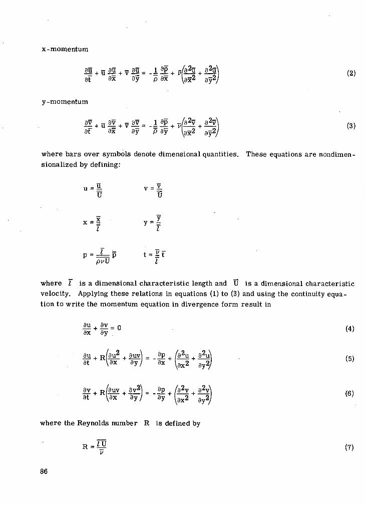
x-momentum
aF + U 9x + ay p ax + "^x2 + ay2/
y-momentum
af + uaf + v a f~ ~/5 af + "( p + ~^2j
where bars over symbols denote dimensional quantities. These equations are nondimen-sionalized by defining:
U U
V Vx ' f y = f
P = ==PpvV
where I is a dimensional characteristic length and U is a dimensional characteristicvelocity. Applying these relations in equations (1) to (3) and using the continuity equa-tion to write the momentum equation in divergence form result in
9u 9v r\ax + ^y ~ ^ '
oluvl -_ x- + i^ ^> +
ax 2 9y2/
9Y + R auv+ K +a t a x a y a y X 2 d y 2
where the Reynolds number R is defined by
R=^ (7)
86
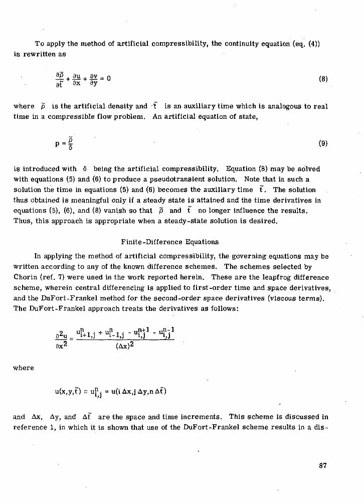
To apply the method of artificial compressibility, the continuity equation (eq. (4))is rewritten as
v = (8)
where p is the artificial density and •'t is an auxiliary time which is analogous to realtime in a compressible flow problem. An artificial equation of state,
(9)
is introduced with 6 being the artificial compressibility. Equation (8) may be solvedwith equations (5) and (6) to produce a pseudotransient solution. Note that in such asolution the time in equations (5) and (6) becomes the auxiliary time f . The solutionthus obtained is meaningful only if a steady state is attained and the time derivatives inequations (5), (6), and (8) vanish so that p and F no longer influence the results.Thus, this approach is appropriate when a steady-state solution is desired.
Finite -Difference Equations
In applying the method of artificial compressibility, the governing equations may bewritten according to any of the known difference schemes. The schemes selected byChorin (ref . 7) were used in the work reported herein. These are the leapfrog differencescheme, wherein central differencing is applied to first-order time and space derivatives,and the DuFort-Frankel method for the second-order space derivatives (viscous terms).The DuFort-Frankel approach treats the derivatives as follows:
9 uP i • + uP -, • - uJH1 - u""19 2 U _ ui+l,] +u i - l> 3 "1,3 ui,38x2 (Ax)2
where
u(x,y,t) s uf; = u(iAx,j Ay,nAt)L>i
and Ax, Ay, and Af are the space and time increments. This scheme is discussed inreference 1, in which it is shown that use of the DuFort-Frankel scheme results in a dis-
87
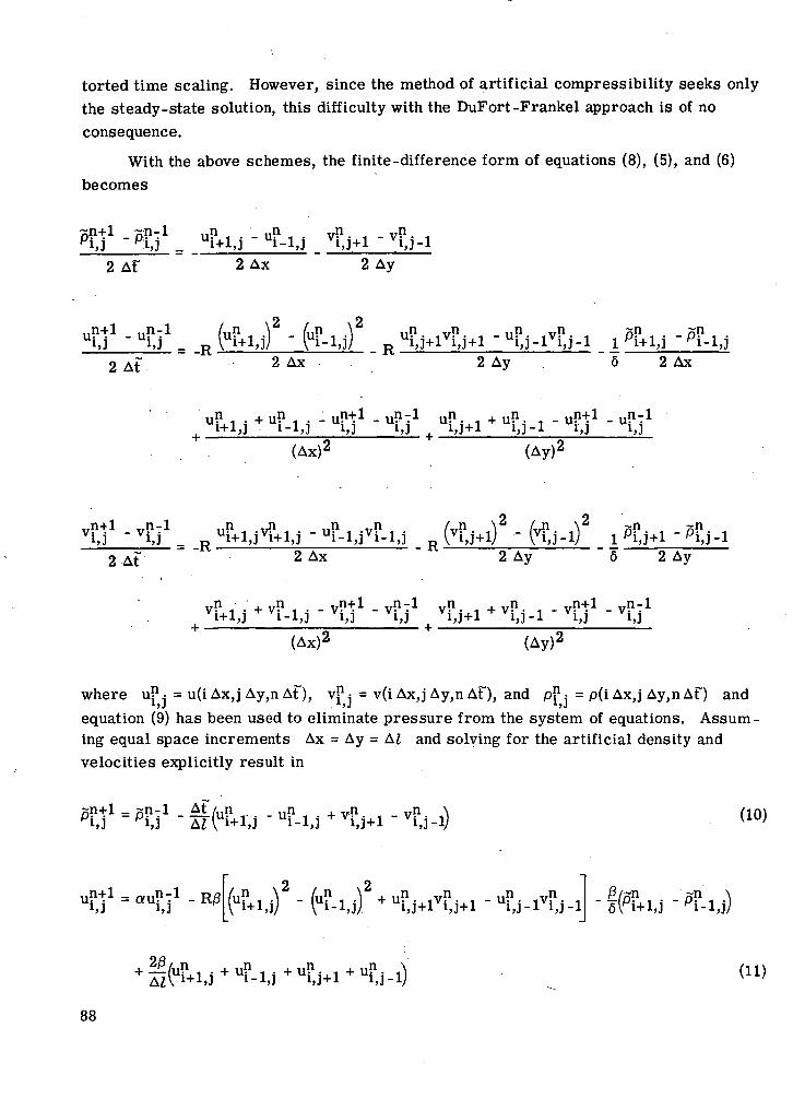
torted time scaling. However, since the method of artificial compressibility seeks onlythe steady-state solution, this difficulty with the DuFort-Frankel approach is of noconsequence.
With the above schemes, the finite -difference form of equations (8), (5), and (6)becomes
+1 _ oP'1,l p:i,3 =
2 AF 2 Ax 2 Ay
2 At
,. ,, ,, ,,ui,j+ivi,j+i -ui,j-ivy-i2 Ax 2 Ay 6 2 Ax
un , un un+l un~l un
i+l,i i-l,i i,i i,i i,i+l2L., . 'J 'J 'J 4. 'Jn n+1 n-1
+ UiJ-l Ui',j Ui,j(Ax)' (Ay)'
_vi,3 ^
2 At= -R
2 Ax,
"2 Ay
rin
2 Ay
VP , - + vP
(Ax)'
VP • , + vP •
(Ay)'
where uP. = u(i Ax,j Ay,n AF), v-^ = v(i Ax,j Ay,n Af), and pP. = p(i Ax,j Ay,n Af) andl)j . 1>J l)Jequation (9) has been used to eliminate pressure from the system of equations. Assuming equal space increments Ax = Ay = A£ and solving for the artificial density andvelocities explicitly result in
i,3 ' A T i + l , Jn (10)
+ uP • ,vP. , - uP .
,T (U (11)
88
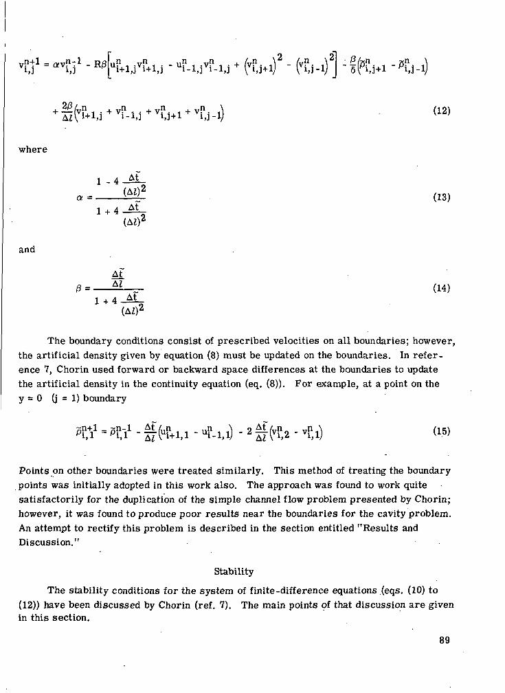
- f
where
(13)
(AZ)2
and
0 = *L__ (14)1 , 4 At
(AZ)2
The boundary conditions consist of prescribed velocities on all boundaries; however,the artificial density given by equation (8) must be updated on the boundaries. In refer-ence 7, Chorin used forward or backward space differences at the boundaries to updatethe artificial density in the continuity equation (eq. (8)). For example, at a point on they = 0 (j = 1) boundary
.2^1
Points on other boundaries were treated similarly. This method of treating the boundarypoints was initially adopted in this work also. The approach was found to work quitesatisfactorily for the duplication of the simple channel flow problem presented by Chorin;however, it was found to produce poor results near the boundaries for the cavity problem.An attempt to rectify this problem is described in the section entitled "Results andDiscussion."
Stability
The stability conditions for the system of finite-difference equations .(eqs. (10) to(12)) have been discussed by Chorin (ref. 7). The main points of that discussion are givenin this section.
89
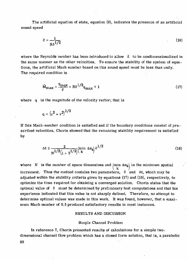
The artificial equation of state, equation (9), indicates the presence of an artificialsound speed
where the Reynolds number has been introduced to allow c to be nondimensionalized inthe same manner as the other velocities. To ensure the stability of the system of equa-tions, the artificial Mach number based on this sound speed must be less than unity.The required condition is
where q is the magnitude of the velocity vector; that is
/ 2 2^/2q = (u2 + v2)
If this Mach-number condition is satisfied and if the boundary conditions consist of pre-scribed velocities, Chorin showed that the remaining stability requirement is satisfiedby
> X /2 (18)- /minN l /2 ( l + 5 l /2)(k
where N is the number of space dimensions and /min Ax^N is the minimum spatialV k }
increment. Thus the method contains two parameters, 6 and At, which may beadjusted within the stability criteria given by equations (17) and (18), respectively, tooptimize the time required for obtaining a converged solution. Chorin states that theoptimal value of 6 must be determined by preliminary test computations and that hisexperience indicated that this value is not sharply defined. Therefore, no attempt todetermine optimal values was made in this work. It was found, however, that a maxi-mum Mach number of 0.5 produced satisfactory results in most instances.
RESULTS AND DISCUSSION
Simple Channel Problem
In reference 7, Chorin presented results of calculations for a simple two-dimensional channel flow problem which has a closed form solution, that is, a parabolic
90
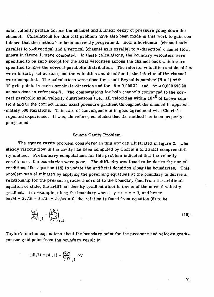
axial velocity profile across the channel and a linear decay of pressure going down thechannel. Calculations for this test problem have also been made in this work to gain con-fidence that the method has been correctly programed. Both a horizontal (channel axisparallel to x-direction) and a vertical (channel axis parallel to y-direction) channel flow,shown in figure 1, were computed. In these calculations, the boundary velocities werespecified to be zero except for the axial velocities across the channel ends which werespecified to have the correct parabolic distribution. The interior velocities and densitieswere initially set at zero, and the velocities and densities in the interior of the channelwere computed. The calculations were done for a unit Reynolds .number (R = 1) with19 grid points in each coordinate direction and for 6 = 0.000 32 and At = 0.000 596 28as was done in reference 7. The computations for both channels converged to the cor-rect parabolic axial velocity distributions (i.e., all velocities within 10"^ of known solu-tion) and to the correct linear axial pressure gradient throughout the channel in approxi-mately 500 iterations. This rate of convergence is in good agreement with Chorin'sreported experience. It was, therefore, concluded that the method has been properlyprogramed.
Square Cavity Problem
The square cavity problem considered in this work is illustrated in figure 2. Thesteady viscous flow in the cavity has been computed by Chorin's artificial compressibil-ity method. Preliminary computations for this problem indicated that the velocityresults near the boundaries were poor. The difficulty was found to be due to the use ofconditions like equation (15) to update the artificial densities along the boundaries. Thisproblem was eliminated by applying the governing equations at the boundary to derive arelationship for the pressure gradient normal to the boundary (and from the artificialequation of state, the artificial density gradient also) in terms of the normal velocitygradient. For example, along the boundary where y = u = v = 0, and hence9u/9t = 9v/8t = 8u/8x = dv/dx = 0, the relation is found from equation (6) to be
(19)
Taylor's series expansions about the boundary point for the pressure and velocity gradi-ent one grid point from the boundary result in
Ayay/i,i
91
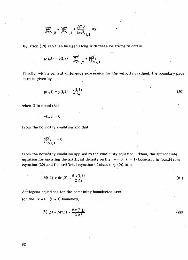
Ay| j "
Equation (19) can then be used along with these relations to obtain
Finally, with a central -difference expression for the velocity gradient, the boundary pres-sure is given by . .-
(20), ,
when it is noted that
v(i,l) = 0
from the boundary condition and that
from the boundary condition applied to the continuity equation. Thus, the appropriateequation for updating the artificial density on the y = 0 (j = 1) boundary is found fromequation (20) and the artificial equation of state (eq. (9)) to be
(21)
.Analogous equations for the remaining boundaries are:
for the x = 0 (i = 1) boundary,
(22)
92
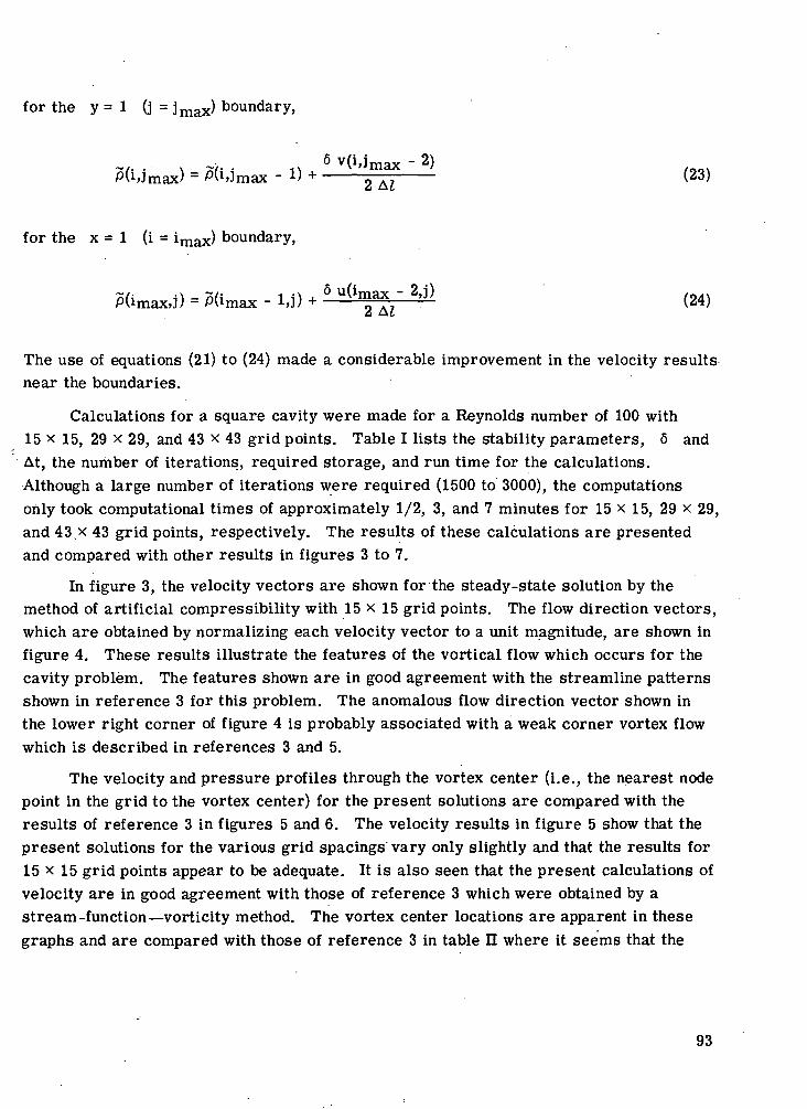
for the y = 1 (j = j max) boundary,
6 vfi.imciY - 2)P(Umax) = fllJmax - D + 2 A? - (23)
for the x = 1 (i = imax) boundary,
~/= i\ - 7>t; t i\ j.PUmax,]) = PUmax - l,)> +
The use of equations (21) to (24) made a considerable improvement in the velocity resultsnear the boundaries.
Calculations for a square cavity were made for a Reynolds number of 100 with15 x 15, 29 x 29, and 43 x 43 grid points. Table I lists the stability parameters, 6 andAt, the number of iterations, required storage, and run time for the calculations.Although a large number of iterations were required (1500 to 3000), the computationsonly took computational times of approximately 1/2, 3, and 7 minutes for 15 x 15, 29 x 29,and 43.x 43 grid points, respectively. The results of these calculations are presentedand compared with other results in figures 3 to 7.
In figure 3, the velocity vectors are shown for the steady-state solution by themethod of artificial compressibility with 15 x 15 grid points. The flow direction vectors,which are obtained by normalizing each velocity vector to a unit magnitude, are shown infigure 4. These results illustrate the features of the vortical flow which occurs for thecavity problem. The features shown are in good agreement with the streamline patternsshown in reference 3 for this problem. The anomalous flow direction vector shown inthe lower right corner of figure 4 is probably associated with a weak corner vortex flowwhich is described in references 3 and 5.
The velocity and pressure profiles through the vortex center (i.e., the nearest nodepoint in the grid to the vortex center) for the present solutions are compared with theresults of reference 3 in figures 5 and 6. The velocity results in figure 5 show that thepresent solutions for the various grid spacings vary only slightly and that the results for15x15 grid points appear to be adequate. It is also seen that the present calculations ofvelocity are in good agreement with those of reference 3 which were obtained by astream -function — vorticity method. The vortex center locations are apparent in thesegraphs and are compared with those of reference 3 in table n where it seems that the
93
values are in good agreement, that is, within about 4 percent. On the other hand, thepressure profiles through the vortex center shown in figure 6 are in substantial disagree -ment. Of particular concern is the fact that the pressure profiles for the various gridspacings of the artificial compressibility method are not smooth and are in disagreementwith each other. This makes the pressure results of this method highly questionable.
In figure 7, the pressures along the boundaries are compared qualitatively with theresults in reference 6. Note that the Reynolds numbers are not the same, that is, 100compared with 64. Although there are relatively high frequency oscillations in the pres-ent results, the qualitative comparisons show good agreement with reference 6.
Thus, these results indicate that the method of artificial compressibility applied tothe square cavity problem produces good results for velocity, but the pressure resultsare unreliable.
CONCLUDING REMARKS
The method of artificial compressibility has been applied to obtain numerical solu-tions of the steady viscous flow in a two-dimensional square cavity. The method, pro-posed by A. J. Chorin, was programed and checked against a simple channel flow problemwhich has an analytic solution. The comparison indicates that the method was correctlyprogramed. Results for a square cavity with a Reynolds number of 100 were obtainedand compared with published solutions for this problem. These comparisons indicatedthat good velocity results are obtained with the method, but that the pressure results areunreliable.
94
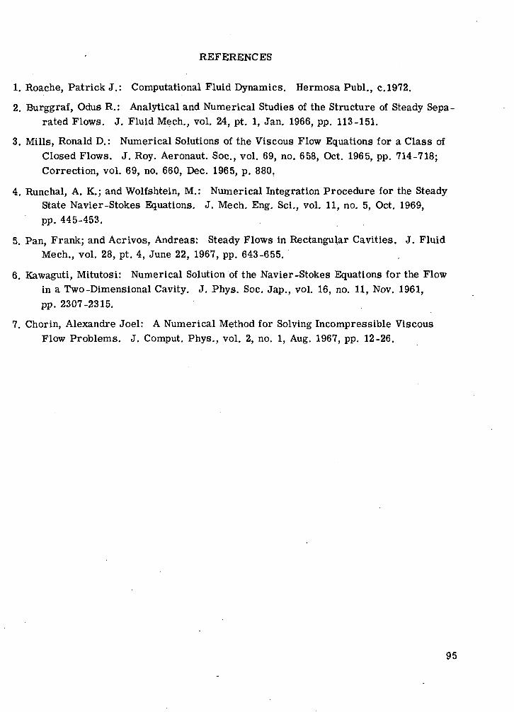
REFERENCES
1. Roache, Patrick J.: Computational Fluid Dynamics. Hermosa Publ., c.1972.
2. Burggraf, Odus R.: Analytical and Numerical Studies of the Structure of Steady Sepa-rated Flows. J. Fluid Mech., vol. 24, pt. 1, Jan. 1966, pp. 113-151.
3. Mills, Ronald D.: Numerical Solutions of the Viscous Flow Equations for a Class ofClosed Flows. J. Roy. Aeronaut. Soc., vol. 69, no. 658, Oct. 1965, pp. 714-718;Correction, vol. 69, no. 660, Dec. 1965, p. 880.
4. Runchal, A. K.; and Wolfshtein, M.: Numerical Integration Procedure for the SteadyState Navier-Stokes Equations. J. Mech. Eng. Sci., vol. 11, no. 5, Oct. 1969,pp. 445-453.
5. Pan, Frank; and Acrivos, Andreas: Steady Flows in Rectangular Cavities. J. FluidMech., vol. 28, pt. 4, June 22, 1967, pp. 643-655.
6. Kawaguti, Mitutosi: Numerical Solution of the Navier-Stokes Equations for the Flowin a Two-Dimensional Cavity. J. Phys. Soc. Jap., vol. 16, no. 11, Nov. 1961,pp. 2307-2315.
7. Chorin, Alexandra Joel: A Numerical Method for Solving Incompressible ViscousFlow Problems. J. Comput. Phys., vol. 2, no. 1, Aug. 1967, pp. 12-26.
95
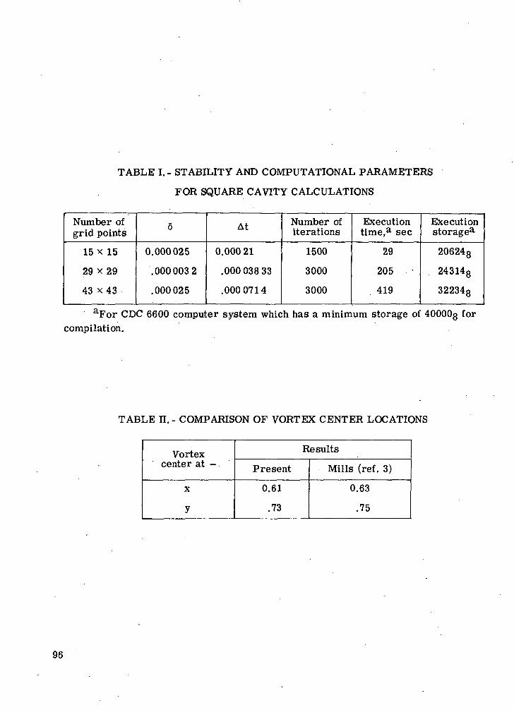
TABLE I. - STABILITY AND COMPUTATIONAL PARAMETERS
FOR SQUARE CAVITY CALCULATIONS
Number ofgrid points
15 x 15
29 x29
43 x 43
6
0.000025
.0000032
.000025
At
0.000 21
.00003833
.0000714
Number ofiterations
1500
3000
3000
Executiontime,a sec
29
205
419
Executionstorage3-
206248
243148
322348
aFor CDC 6600 computer system which has a minimum storage of 40000g forcompilation.
TABLE H.- COMPARISON OF VORTEX CENTER LOCATIONS
Vortexcenter at -
x
y
Results
Present
0.61
.73
Mills (ref. 3)
0.63
.75
96
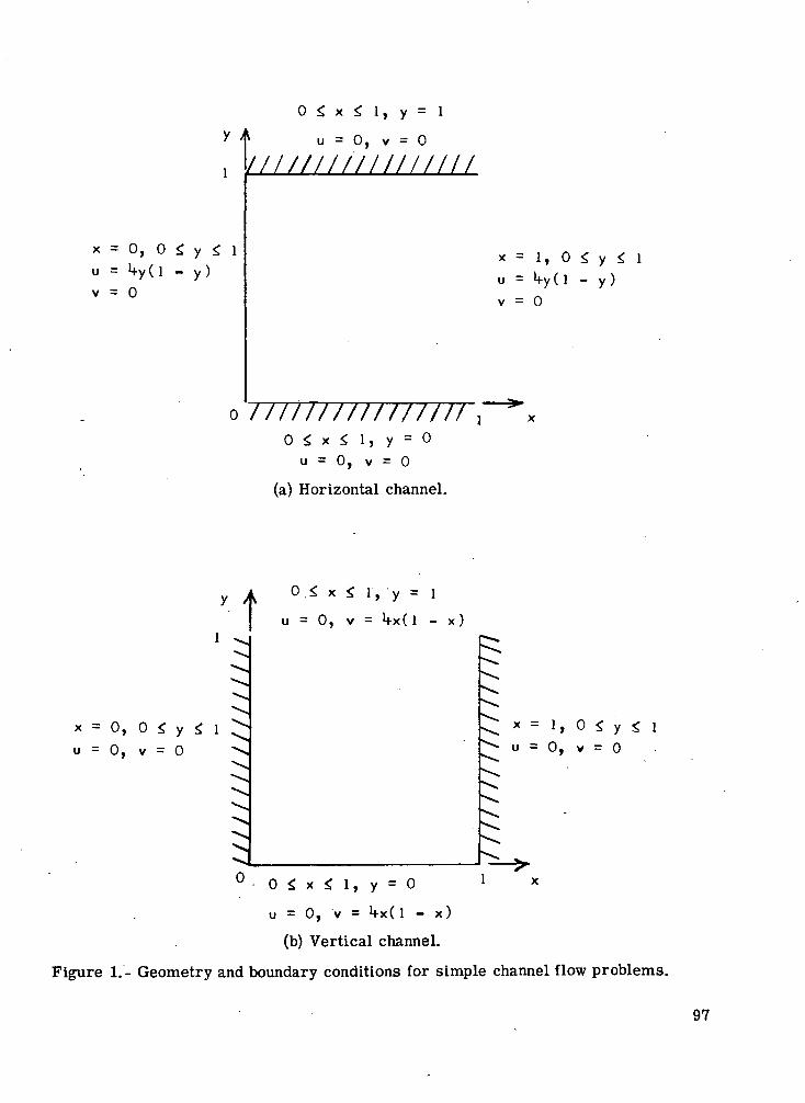
x = 0, 0 £ y
u = "+yU - y)
v = 0
0 £ x £ 1, y = 1
u = 0, v = 0
ni///t/n innn
0 / / / / / / / / / / / / / / / /
0 £ x * l , y = 0
u = 0, v = 0
(a) Horizontal channel.
x = 1, 0 £ y
U = lfy(l - y )
V = 0
x = 0, 0 <. yu = 0, v = 0
y A O.S x £ 1, y = i
u = 0, v = >+x( 1 - x)
x = 1, 0 <. y <, I
u = 0, v = 0
0 - 0 S x * 1, y=0 ! x
u = 0, v = *tx( 1 - x)
(b) Vertical channel.
Figure 1. - Geometry and boundary conditions for simple channel flow problems.
97
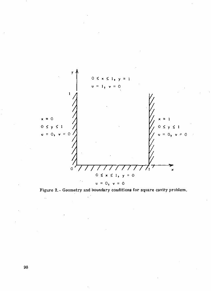
u = 0, v = 0 /,
0 * x * 1, y = 1
u = 1, v = 0
I-A o <; y <: iy u = o, v = oi
O V / / / / / / / / / / / 1 7 x
O ^ x ^ l , y = 0
u = 0, v = 0Figure 2.- Geometry and boundary conditions for square cavity problem.
98
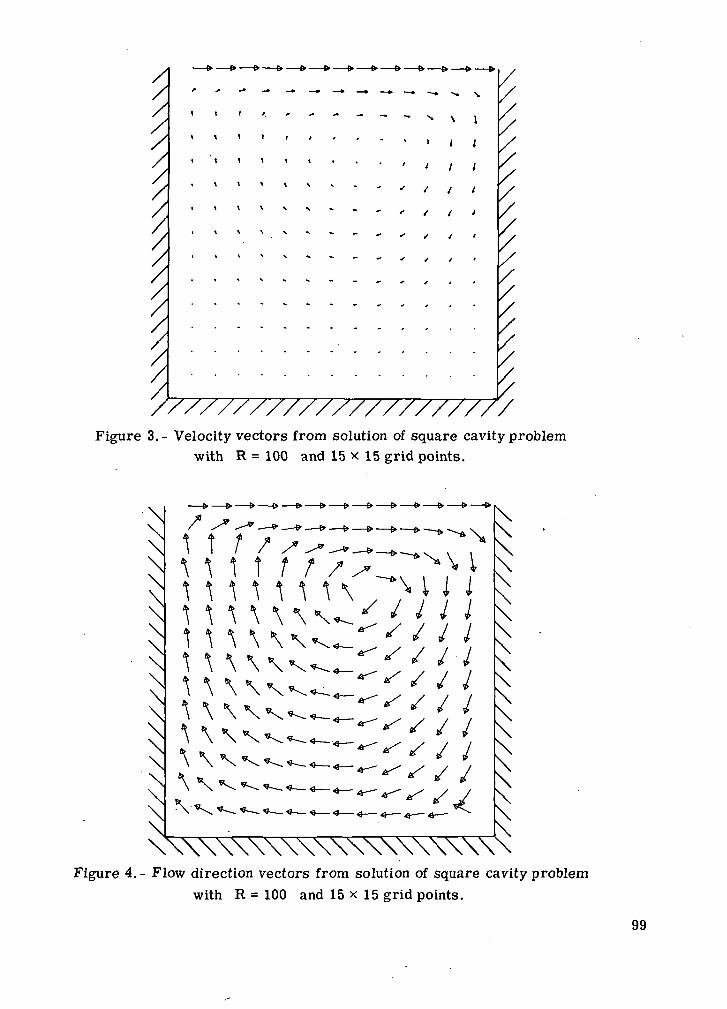
X/////'//,r//,','/','/
t i » / f * ~ . » - • _ . .- •* \ i, , i
1 ' ' / / i* * ^ * - - • • / / /
" • • / / <" * / / *
^X/X//////V/
//'/
Figure 3.- Velocity vectors from solution of square cavity problemwith R = 100 and 15 * 15 grid points.
Figure 4.- Flow direction vectors from solution of square cavity problemwith R = 100 and 15x15 grid points.
99
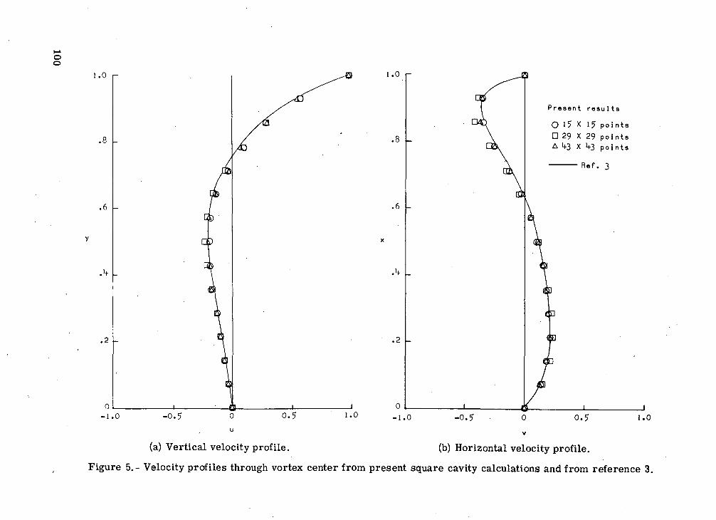
f-tmt>*•conou0.
1
OD.
IfN.
~~
Xlr\r-l
0
O
o
roa.
a.O
N
ro <
^CM
J-
•>oc —
X
X
ON ro
OH J-
n , H
@
— ,
J3
^^r-^^
w
- ^^\J
ITN
Or^i
0)f—
I.•ri
M-l
OQ.
>,
(Up—4
IOStO
0)o20)soT3rtCO§3•ao
ITN•
O
flo
0)Sia*wenSoa>oXa>
S
-c^<
bDO<
^
O
S
3
nCD
0)>
:±
oCD>i:>
ft>>-<->-^OOiITS
°7
100

O
oo
IIaoo^HaOS3
o>oc0)ao73CrtCQO3"3o
" 1C(Uin(Uco(1)U
~<
O-
<no
_o
"5T
Suo
"oT
O!HaIHrto4->VlCD>'rt
Ibfisc0)(Uou3COCQ(Da•sCQ
co101
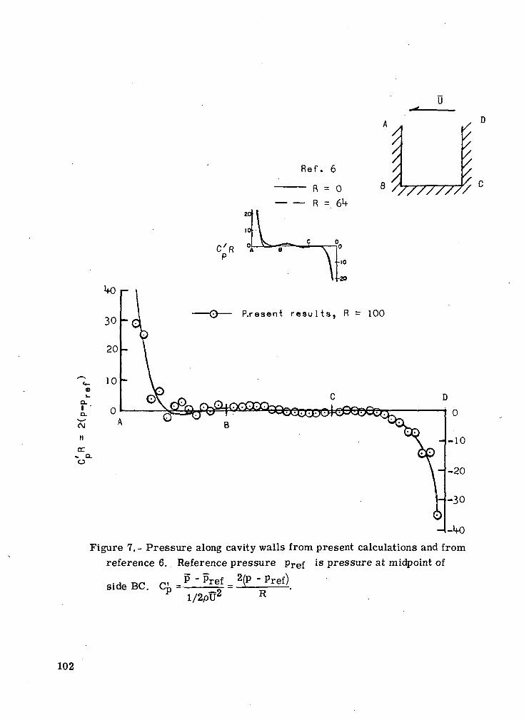
o.IQ.
>«x
CVJ
IIcc.
~. Q.o
Ref. 6
R = 6tf20
10
C'R
\"lf-20
P.resent r e s u l t s , R = 100
-30
-1-1*0
Figure 7.- Pressure along cavity walls from present calculations and fromreference 6. Reference pressure pref is pressure at midpoint of
„ _ P - Pref _ 2(P - Pref)'P ~ ^9 T? *
l/2ptr Kside BC.
102
8. FINITE-DIFFERENCE SOLUTION FOR THE INCOMPRESSIBLE
DRIVEN CAVITY FLOW PROBLEM
Ernest V. ZobyLangley Research Center
SUMMARY
An alternating-direction implicit (ADI) finite-difference procedure has beenemployed to compute the two-dimensional viscous incompressible flow generated withina rectangular cavity by a moving surface at the cavity open end. The pressure throughthe cavity was computed by the Spalding SIMPLE procedure.
Although the present method does not predict axial and normal velocities as highas indicated by more exact methods, the values of the velocities through the vortex cen-ter are reasonably predicted and the overall velocity vector diagrams appear satisfac-tory. The pressure levels are generally in poor agreement with other predictions.However, the pressure gradients must be reasonably well predicted because of the accu-rate results obtained for the velocities.
INTRODUCTION
The solution of the Navier-Stokes equations easily provides a more than adequatetest for the viability of various numerical techniques. For a rational assessment ofthese methods, a singular flow model and compatible test conditions are naturally desir-able. Numerical as well as experimental results (e.g., ref. 1) exist for the two-dimensional incompressible flow field generated within a rectangular cavity by a movingsurface at the open end. (See paper no. 1 by Rubin and Harris for details of driven cav-ity.) Consequently, the driven cavity problem was selected as the test model for aninvestigation to compare the accuracy and applicability of several numerical techniques.
As part of the aforementioned investigation, this paper presents numerical solu-tions based on an alternating-direction implicit (ADI) technique for the two-dimensionalincompressible Navier-Stokes equations. The equations are programed in the rectangu-lar Cartesian coordinate system. For an evaluation of the pressure, the SpaldingSIMPLE procedure (ref. 2) is used. The Spalding method relates a perturbation in pres-sure at each time step to the continuity relation so that at steady state the pressure ateach node point is determined and the continuity equation is satisfied. A discussion of
103
the present method and the results of calculated test cases are presented. Comparisonwith existing results is also included.
SYMBOLS
Cp pressure coefficient
I characteristic length (fig. 1)
p pressure
p pressure correction
R Reynolds number —
t time
At time step
U velocity across open end of cavity
u axial component of velocity
v normal component of velocity
x,y axial and normal distance, respectively
Ax,Ay spatial increments in x-and y-directions
D kinematic viscosity
p density
Subscripts:
i,j index of node points in x- and y-direction, respectively
max maximum value
104
Superscripts:
k iteration counter
n index of time step
A bar over a symbol denotes a dimensional quantity.
ANALYSIS
The governing equations for an incompressible viscous fluid in two-dimensionalrectangular coordinates are given as
+ u + v= + + ) (1)at ax ay p ax \ax2 ay2/
at ax ay p ay yax2 ay2/
and
au av _ Q /o\af af ~
Defining the dimensionless quantities to be
x = I y = II I
U U
and substituting them into equations (1) to (3) result in
9H + u^ + v^= _^E + I/ i + l!li\ (4)at ax+ v ay 9x+ RLX2 ay2/ v '
105
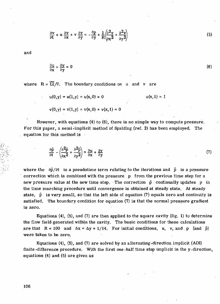
and
3u . 3v n (c\1- = U 10)ax ay
where R = UZ/F. The boundary conditions on u and v are
u(0,y) = u(l,y) = u(x,0) = 0 u(x,l) = 1
v(0,y) = v(l,y) = v(x,0) = v(x,l) = 0
However, with equations (4) to (6), there is no simple way to compute pressure.For this paper, a semi-implicit method of Spalding (ref. 2) has been employed. Theequation for this method is -
ax ay
where the ap/9t is a pseudotime term relating to the iterations and p is a pressurecorrection which is combined with the pressure p from the previous time step for anew pressure value at the new time step. The correction p continually updates p inthe time marching procedure until convergence is obtained at steady state. At steadystate, p is very small, so that the left side of equation (7) equals zero and continuity issatisfied. The boundary condition for equation (7) is that the normal pressure gradientis zero.
Equations (4), (5), and (7) are then applied to the square cavity (fig. 1) to determinethe flow field generated within the cavity. The basic conditions for these calculationsare that R = 100 and Ax = Ay = 1/14. For initial conditions, u, v, and p (and p)were taken to be zero.
Equations (4), (5), and (7) are solved by an alternating-direction implicit (ADI)finite -difference procedure. With the first one -half time step implicit in the y-direction,equations (4) and (5) are given as
106
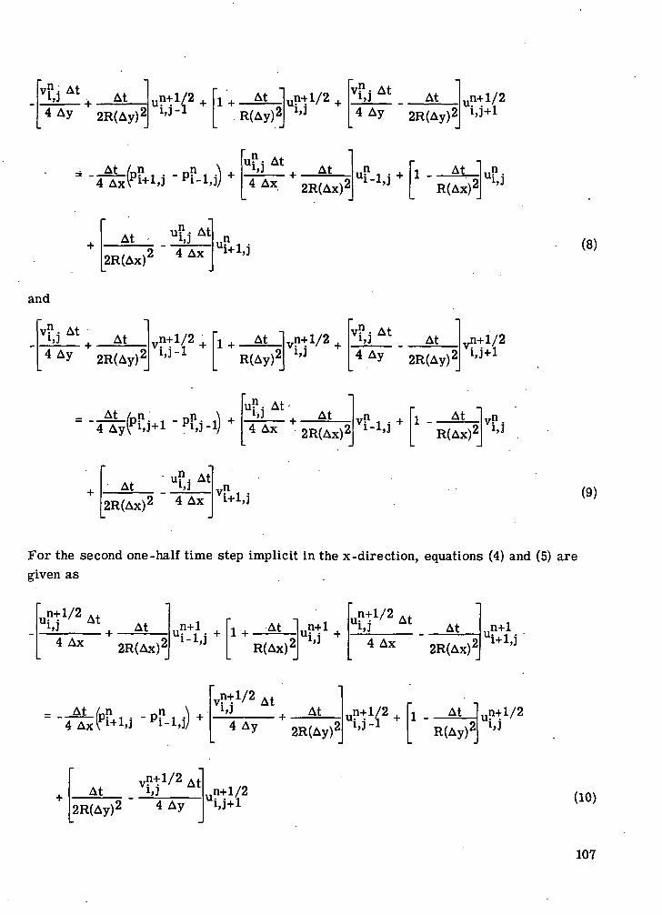
,n At
4 Ay 2R(Ay)2
At4 Ax
1 + At
R(Ay)2Ji,j
At2R(Ay)2
n At
2R(Ax)2 R(Ax)'
At
2R(Ax)2 4 Ax
and
U A t , At
2R(Ay)
A t n ; _ n .
R(Ay)2JAt%j At
4 Ay 2R(Ay)2
atAt
2R(Ax)2At
T,J
AtAt
2R(Ax)2 4 Ax
(8)
(9)
For the second one-half time step implicit in the x-direction, equations (4) and (5) aregiven as
At4 Ax 2R(Ax)2
1 + At
R(Ax)'
At
2R(Ax)2
n+1
._A^/Un4 Ax1
v-tl /2 AtAt
2R(Ay)21 - At
R(Ay)'
At2R(Ay)2 4 Ay
uPt1/2u (10)
107
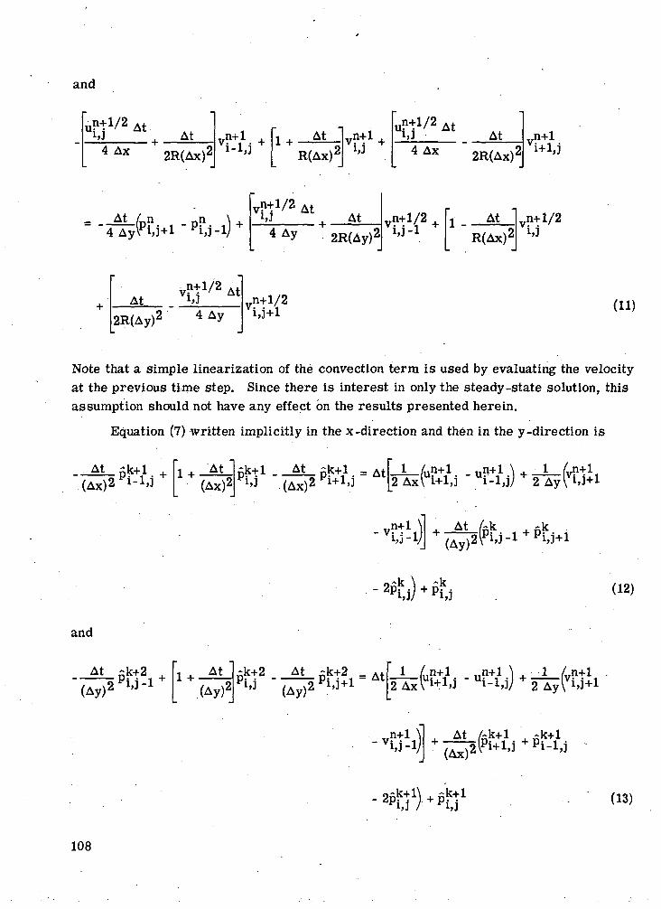
and
"un+l/2Ui,j At
At4 Ax 2R(Ax)2
1 + At
R(Ax):
At4 Ax 2R(Ax)2
n+1V
_ At At4 Ay 2R(Ay)'
1 - At
R(Ax)'n+l/2v
At2R(Ay)2
Tn+l/2 (11)
Note that a simple linearization of the convection term is used by evaluating the velocityat the previous time step. Since there is interest in only the steady-state solution, thisassumption should not have any effect on the results presented herein.
Equation (7) written implicitly in the x-direction and then in the y-direction is
pk+1 . AtPI,] (Ax)2(Ax)2
_At_/pk + p-k( A y )2\U-l i,
i,j-k (12)
and
At -k+2(Ay)'
1 + At
(Ay)'
-k+2 At -k+2 _- - n+1
(13)
108
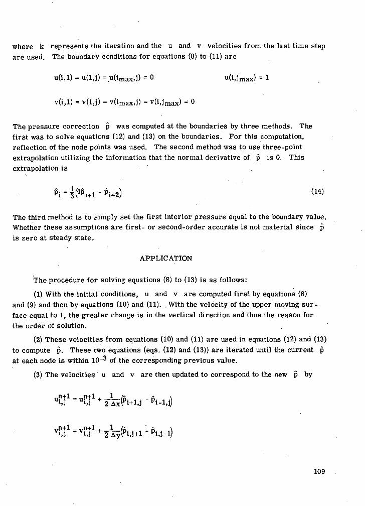
where k represents the iteration and the u and v velocities from the last time stepare used. The boundary conditions for equations (8) to (11) are
u(i,l) = u(l,j) = u(imax,j) = 0 u(i,jmax) = 1
v(i,l) = v(l,j) = v(imax,j) = v(i,jmax) = 0
The pressure correction p was computed at the boundaries by three methods. Thefirst was to solve equations (12) and (13) on the boundaries. For this computation,reflection of the node points was used. The second method was to use three-pointextrapolation utilizing the information that the normal derivative of p is 0. Thisextrapolation is
The third method is to simply set the first interior pressure equal to the boundary value.Whether these assumptions are first- or second-order accurate is not material since pis zero at steady state.
APPLICATION
The procedure for solving equations (8) to (13) is as follows:
(1) With the initial conditions, u and v are computed first by equations (8)and (9) and then by equations (10) and (11). With the velocity of the upper moving sur-face equal to 1, the greater change is in the vertical direction and thus the reason forthe order of solution.
(2) These velocities from equations (10) and (11) are used in equations (12) and (13)to compute p. These two equations (eqs. (12) and (13)) are iterated until the current pat each node is within 10"^ of the corresponding previous value.
(3) The velocities u and v are then updated to correspond to the new p by
109
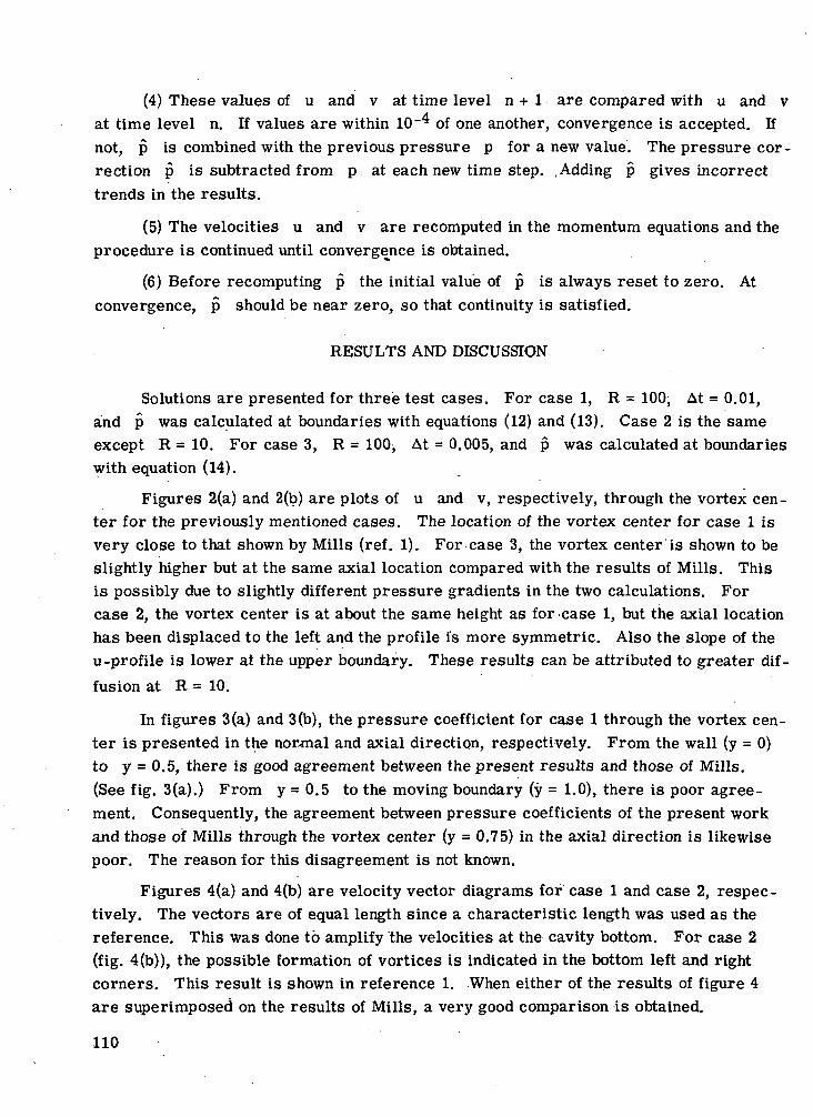
(4) These values of u and v at time level n + 1 are compared with u and vat time level n. If values are within 10 ~^ of one another, convergence is accepted. Ifnot, p is combined with the previous pressure p for a new value. The pressure cor-rection p is subtracted from p at each new time step. .Adding p gives incorrecttrends in the results.
(5) The velocities u and v are recomputed in the momentum equations and theprocedure is continued until convergence is obtained.
(6) Before recomputing p the initial value of p is always reset to zero. Atconvergence, p should be near zero, so that continuity is satisfied.
RESULTS AND DISCUSSION
Solutions are presented for three test cases. For case 1, R = 100, At = 0.01,and p was calculated at boundaries with equations (12) and (13). Case 2 is the sameexcept R = 10. For case 3, R = 100> At = 0.005, and p was calculated at boundarieswith equation (14).
Figures 2(a) and 2(b) are plots of u and v, respectively, through the vortex cen-ter for the previously mentioned cases. The location of the vortex center for case 1 isvery close to that shown by Mills (ref. 1). For case 3, the vortex center is shown to beslightly higher but at the same axial location compared with the results of Mills. Thisis possibly due to slightly different pressure gradients in the two calculations. Forcase 2, the vortex center is at about the same height as for-case 1, but the axial locationhas been displaced to the left and the profile is more symmetric. Also the slope of theu-profile is lower at the upper boundary. These results can be attributed to greater dif-fusion at R = 10.
In figures 3(a) and 3(b), the pressure coefficient for case 1 through the vortex cen-ter is presented in the normal and axial direction, respectively. From the wall (y = 0)to y = 0.5, there is good agreement between the present results and those of Mills.(See fig. 3(a).) From y = 0.5 to the moving boundary (y = 1.0), there is poor agree-ment. Consequently, the agreement between pressure coefficients of the present workand those of Mills through the vortex center (y = 0.75) in the axial direction is likewisepoor. The reason for this disagreement is not known.
Figures 4(a) and 4(b) are velocity vector diagrams for case 1 and case 2, respec-tively. The vectors are of equal length since a characteristic length was used as thereference. This was done to amplify the velocities at the cavity bottom. For case 2(fig. 4(b)), the possible formation of vortices is indicated in the bottom left and rightcorners. This result is shown in reference 1. When either of the results of figure 4are superimposed on the results of Mills, a very good comparison is obtained.
110
A note may be made of the pressure gradients through the cavity. In figure 3, thepressures are generally in poor agreement with published results. However, consider-ing the good agreement obtained for the velocities in figures 2 and 4, it is assumed thatthe pressure gradients computed in the present analysis must be reasonably wellpredicted.
Other conditions were considered in investigating this problem. Solving for p onthe boundaries by the third method discussed previously (e.g., p(l,j) = p(2,j)) resulted invalues for u, v, and p which were not in good agreement with results obtained bycomputing p at the boundaries by equations (12) and (13) or by equation (14). A con-vergence criterion on u and v of 10'"* rather than 10"** gave much better agreementwith results of reference 1. Convergence could not be obtained if accuracy on p wasraised from 10-3 to 10~4.
For any of the applications, the values of u and v are not iterated to a requiredconvergence at each time step. Convergence is only tested for the values at the currentand previous time steps. This type of time marching would only produce convergence atsteady state, and the transient results are not accurate.
Since most of the documented results on this flow problem are presented in termsof stream-function—vorticity variables, an overall comparison of the present resultscomputed in primitive variables is difficult. However, where at least a cursory com-parison is possible, slightly lower levels for u and v are computed by the methoddiscussed in this paper, and a poor comparison for the pressures is indicated. Thisimplies that the results obtained by the simplified approach presented herein are not soaccurate as the results obtained by a more rigorous analysis.
CONCLUDING REMARKS
An alternating-direction implicit (ADI) finite-difference procedure has beenemployed to compute the two-dimensional viscous incompressible flow generated withina rectangular cavity by a moving surface at the cavity open end. The pressure throughthe cavity was computed by the Spalding SIMPLE procedure.
Although the present method does not predict axial and normal velocities as highas indicated by the more exact methods, the values of the velocities through the vortexcenter are reasonably predicted and the overall velocity vector diagrams appear satis-factory. The pressure levels are generally in poor agreement with other predictions.However, the pressure gradients must be reasonably well predicted because of the accu-rate results obtained for the velocities.
Ill
REFERENCES
1. Mills, Ronald D.: Numerical Solutions of the Viscous Flow Equations for a Class ofClosed Flows. J. Roy. Aeronaut Soc., vol. 69, no. 658, Oct. 1965, pp. 714-718;Correction, vol. 69, no. 660, Dec. 1965, p. 880.
2. Caretto, L. S.; Gosman, A. D.; Patankar, S. V.; and Spalding, D. B.: Two CalculationProcedures for Steady, Three-Dimensional Flows With Recirculation. Proceedingsof the Third International Conference on Numerical Methods in Fluid Mechanics,Volume n. Volume 19 of Lecture Notes in Physics, Henri Cabannes and RogerTemam, eds., Springer-Verlag, July 1972, pp. 60-68.
112
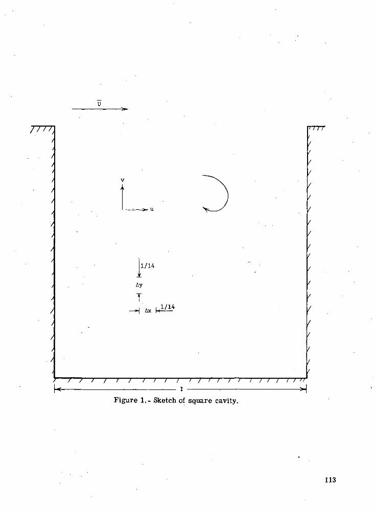
1/14
Ay
T.—H Ax
1/14
/ 7 7 / 7 7 / i I 7 7 * I I T / i f "
Figure 1,- Sketch of square cavity.
113
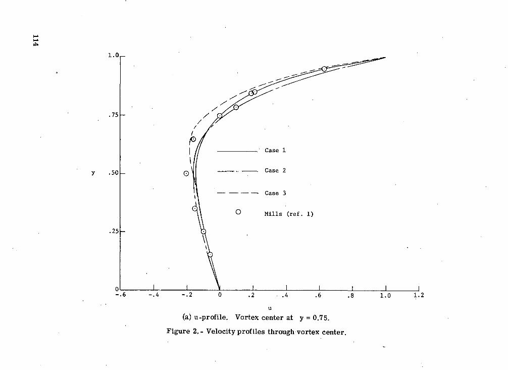
\\\\\\
vOvt
eg•
OCN
irj
oII>>rtMQ)
3
CQ)09•co«>-H
1a3'rt
0)oX0•c0x:bDOF-iX
!"*"enO)
*oa'ooieg'0)b
Lo
114
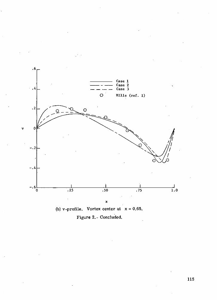
.4
Case 1Case 2Case 3
O Mills (ref. 1)
.2
v 0
-.2
-.4
-.6.25 .50 .75 1.0
(b) v-profile. Vortex center at x = 0.65.
Figure 2.- Concluded.
115
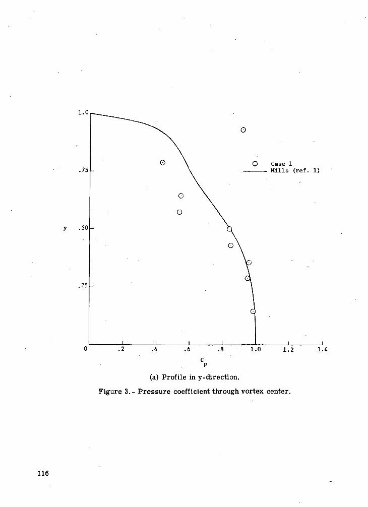
y .50 -
O
O Case 1Mills (ref. 1)
(a) Profile in y-direction.
Figure 3.- Pressure coefficient through vortex center.
1.4
116
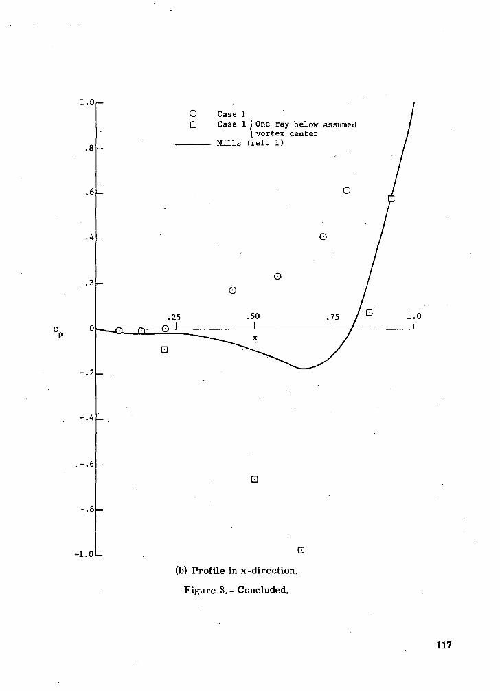
1.0
.8
.6
on
Case 1Case 1 ( One ray below assumed
\ vortex centerMills (ref. 1)
-.21
-.4
.-.6
-.8
-1.01 CD
(b) Profile in x-direction.
Figure 3.- Concluded.
117
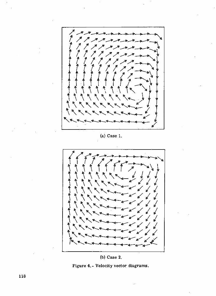
(a) Case 1.
1 I / / / /• s*^—*\\ \\ \ \ f T>, , , ,n \ \ \ \ \ N _ / / / y1J^\ \ \
(b) Case 2.
Figure 4.- Velocity vector diagrams.
118
9. CUBIC SPLINE SOLUTION FOR THE DRIVEN CAVITY
Stanley G. Rubin* and Randolph A. Graves, Jr.Langley Research Center
SUMMARY
A cubic spline procedure for solution of the vorticity—stream-function system forflow in a driven cavity has been described. The spline results were compared with finite-difference results and were found to be more accurate, even near the boundaries. Anonuniform grid was also used with increased mesh density in regions where diffusionwas important. Considerable advantages of the spline procedure with a nonuniform gridwere indicated in regions of large gradients.
INTRODUCTION
The present paper describes a cubic spline procedure for the solution of the drivencavity problem. (See paper no. 1 by Rubin and Harris for details of this problem.) Avorticity—stream-function system is considered. A finite-difference discretization isused for the marching or timelike direction. Unlike a finite-element or Galerkin proce-dure, there are no quadratures to evaluate and the coefficient matrix is tridiagonal. Thespline approximation is second-order accurate even with relatively large variations inthe mesh. Moreover, for the convective terms (first derivatives) the spline procedure isthird-order accurate with a nonuniform mesh and fourth-order accurate with a uniformmesh. A detailed discussion of splines and spline procedures for fluid dynamics can be
found in reference 1.
SYMBOLS
a,b end points of interval
hi,kj mesh widths; x^ - X[_i and yj - yj-1, respectively
L},Mj[ spline second derivative in y- and x-direction,, respectively
f-i,mi spline first derivative in y- and x-direction, respectively
*Visiting professor at Old Dominion University, Norfolk, Va. Now professor ofaerospace engineering, Polytechnic Institute of New York, Farmingdale, N.Y.
119
N number of nodes in interval [a,b] excluding boundaries
R Reynolds number
SA cubic spline function
t time
At time step
u,v axial and normal velocity component, respectively
Xi nodal points
x,y coordinate in axial and normal direction, respectively
£ vorticity
9 index of finite-difference scheme; 0 for explicit, 1/2 for Crank-Nicolson,1 for implicit
T fictitious time
AT fictitious time step
\l/ stream function
Superscripts:
n index of time step At
s index of fictitious time step AT
Subscripts: '
i,j index of nodal points in x- and y-direction, respectively
max maximum
120
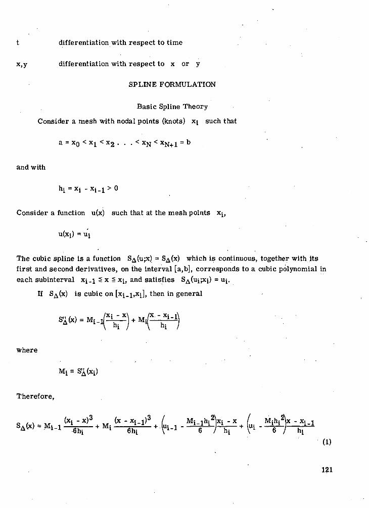
t differentiation with respect to time
x,y differentiation with respect to x or y
SPLINE FORMULATION
Basic Spline Theory
Consider a mesh with nodal points (knots) x[ such that
a = x0 < xx < x2 . . . < XN < xN+1 = b
and with
h i = x i - x i _ 1 > 0
Consider a function u(x) such that at the mesh points Xj,
u(xi) = Ui
The cubic spline is a function SA(UJX) = S^(x) which is continuous, together with itsfirst and second derivatives, on the interval [a,b], corresponds to a cubic polynomial ineach subinterval x[_i S x ^ Xi, and satisfies S^(ui;xi) = u^.
If S^(x) is cubic on [xi_j,xj, then in general
where
Therefore,
(1)
121
The unknown derivatives M^ are related by enforcing the continuity condition onSA(x). With S'(xi-) = mi- on [xj.^xj and SA xf = m* on [Xi,xi+1],
For i = 1, . . ., N,
-^ ,2,
,3,
Equation (2) lead to a system of N equations for the N + 2 unknown M^.
Splines for Solving Partial Differential Equations
If the values u^ are not prescribed but represent the solution of a quasi -linearsecond-order partial differential equation, such as
ut = f (u,ux,uxx)
then an approximate solution for Uj can be obtained by considering the solution of
(ut)i = f(ui>mi>Mi)
where the time derivative is discretized in the usual finite -difference fashion; that is,
n+l n
At- 0)fn
where 9 = 0, 1, and 1/2 for explicit, implicit, and Crank -Nicolson finite -differenceschemes, respectively. The physical time t equals n At (At is the time incrementat each step).
122
For equations with two space dimensions such that
u t = f u ^ u
a spline -alternating -direction -implicit (SADI) formulation is developed. The two-stepprocedure, with quasi -linearization or some other iterative process used for nonlinearterms, is of the following form:
Step 1
_ ,,n . At f Ln+1/2 ,»n+, -UU + T f U m
Step 2
,,n+l _ ,,n+l/2 . At t Ln+1/2 n+1/2 A/rn+l/2 On+l T n+l\u -u + >m M £ L
where H\ \ and L: t are the spline approximations to (uv\ and (\i,,v\ ,i, i,j v y;i,j v yy/i j»respectively.
INCOMPRESSIBLE FLOW IN A CAVITY
Equations
For the driven cavity the governing equations, in terms of vorticity and streamfunction, are
(6)
where i/' is the stream function, £ is the vorticity, and u = i/'y and v = -i//x arethe velocities in the x- and y-directions, respectively. For all calculations the initialconditions are ty(x,y) = 0 and £(x,y) = 0.
Solutions are obtained by the iterative SADI procedure. The SADI system repre-senting equations (6) is given in two steps for both stream function and vorticity.
123
Stream function. - For step 1,
^
n+1,8+1/2 =n+l,s+l/2 , ti\n+1's
) + KJ) (7a)
For step 2,
,,,11+1M.J
,8+1 = AT (7b)
where AT is a fictitious time step and r = s AT. Solutions for equations (6) areobtained as the steady-state limit (T — °o) of equations (7). The notation L[ j and Mi jdenote the spline approximations to a^A/ay^ and a^A/ax^, respectively. (The super-script i// implies that A = i//.) First derivatives i//y = u and i^x = -v are repre-sented by if. and n i j - , respectively.
Vorticity. - For step 1,
cn+l/2 ,.? AtM,.l M,l 9 -£ 4* ,n+l/2 / . Nn+l/2
I j. T? ~1|T = I _i_ T3 •) +R lLiJ +R (8a)
For step 2,
n+1/2 n+l/2 n+l(8b)
The bar over superscript fy in the spline derivatives denotes an average of values attime steps n and n + l. The £ superscript denotes ? spline derivatives.
Numerical Solution Procedure
The iterative procedure is as follows:
(1) With and given either as initial conditions or at time n At, all the> spline derivatives are determined from equations (1) to (4). On the vertical surfaces,
i i = ?i i5 on the horizontal boundaries, Lf ,- = ?; ^.vJ 1>J . 1>J 1>J
124
(2) The vorticity ?y 1 is obtained with the SADI technique outlined by equa-tions (5). At the boundaries, ?y is found from an expression similar to equation (3)or (4). At the upper moving wall (w),
\p , _ ki,wLj,w ki,wLi,w-l M,W " M,w-= 1 =-— 3— + 6 + ~
w-l M,W+
where k = y - y. With t^ = 0 and
Similar relations can be derived for the three stationary walls. Boundary values forM? . and L? . are obtained from equations (8) evaluated at the surface. For the mov-
ing wall, equations (3) and (4) are used to eliminate m?j . In addition, Cf"^/^ is eval-uated with the three-point formula; that is,
(3) The vorticity Cnt is used in equations (7) and the SADI procedure is applied*•>]
over the fictitious time r until a converged solution, to any specified tolerance, isobtained.
(4) If only the steady -state solution is required, the calculation proceeds to thenext time step n + 2 by returning to step (2) with n replacing n + 1 . The splinederivatives for i// have already been determined in step (3).
If an accurate transient solution is required, the calculation proceeds to step (2)with ^ i and all spline derivatives of $ replaced by averages over the n and n+1time steps. Then ^Pt1 is recalculated. This process continues until convergence isreached.
Results
Calculations are presented for a square cavity with R = 100. Comparisons aregiven with finite -difference calculations in both divergence and nondivergence form as
125
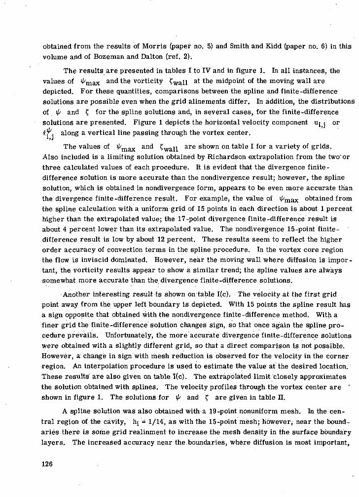
obtained from the results of Morris (paper no. 5) and Smith and Kidd (paper no. 6) in thisvolume and of Bozeman and Dalton (ref. 2).
The results are presented in tables I to IV and in figure 1. In all instances, thevalues of '/'max and the vorticity Cwall a* *ne midpoint of the moving wall aredepicted. For these quantities, comparisons between the spline and finite -differencesolutions are possible even when the grid alinements differ. In addition, the distributionsof 41 and £ for the spline solutions and, in several cases, for the finite-differencesolutions are presented. Figure 1 depicts the horizontal velocity component u^ j or$'. along a vertical line passing through the vortex center.
*>JThe values of i/^^ and £wau are shown on table I for a variety of grids.
Also included is a limiting solution obtained by Richardson extrapolation from the two" orthree calculated values of each procedure. It is evident that the divergence finite -difference solution is more accurate than the nondivergence result; however, the splinesolution, which is obtained in nondivergence form, appears to be even more accurate thanthe divergence finite-difference result. For example, the value of i^max obtained fromthe spline calculation with a uniform grid of 15 points in each direction is about 1 percenthigher than the extrapolated value; the 17-point divergence finite-difference result isabout 4 percent lower than its extrapolated value. The nondivergence 15-point finite-difference result is low by about 12 percent. These results seem to reflect the higherorder accuracy of convection terms in the spline procedure. In the vortex core regionthe flow is inviscid dominated. However, near the moving wall where diffusion is impor-tant, the vorticity results appear to show a similar trend; the spline values are alwayssomewhat more accurate than the divergence finite-difference solutions.
Another interesting result is shown on table I(c). The velocity at the first gridpoint away from the upper left boundary is depicted. With 15 points the spline result hasa sign opposite that obtained with the nondivergence finite-difference method. With afiner grid the finite-difference solution changes sign, so that once again the spline pro-cedure prevails. Unfortunately, the more accurate divergence finite-difference solutionswere obtained with a slightly different grid, so that a direct comparison is not possible.However, a change in sign with mesh reduction is observed for the velocity in the cornerregion. An interpolation procedure is used to estimate the value at the desired location.These results are also given on table I(c). The extrapolated limit closely approximatesthe solution obtained with splines. The velocity profiles through the vortex center are 'shown in figure 1. The solutions for 41 and £ are given in table II.
A spline solution was also obtained with a 19-point nonuniform mesh. In the cen-tral region of the cavity, hj = 1/14, as with the 15-point mesh; however, near the bound-aries there is some grid realinment to increase the mesh density in the surface boundarylayers. The increased accuracy near the boundaries, where diffusion is most important,
126
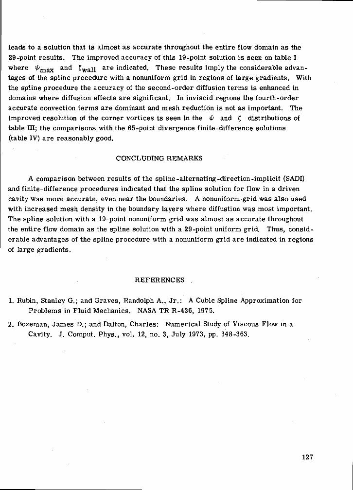
leads to a solution that is almost as accurate throughout the entire flow domain as the29-point results. The improved accuracy of this 19-point solution is seen on table Iwhere ^max and £wau are indicated. These results imply the considerable advan-tages of the spline procedure with a nonuniform grid in regions of large gradients. Withthe spline procedure the accuracy of the second-order diffusion terms is enhanced indomains where diffusion effects are significant. In inviscid regions the fourth-orderaccurate convection terms are dominant and mesh reduction is not as important. Theimproved resolution of the corner vortices is seen in the 4* and £ distributions oftable HI; the comparisons with the 65-point divergence finite-difference solutions(table IV) are reasonably good.
CONCLUDING REMARKS
A comparison between results of the spline-alternating-direction-implicit (SADI)and finite-difference procedures indicated that the spline solution for flow in a drivencavity was more accurate, even near the boundaries. A nonuniform grid was also usedwith increased mesh density in the boundary layers where diffustion was most important.The spline solution with a 19-point nonuniform grid was almost as accurate throughoutthe entire flow domain as the spline solution with a 29-point uniform grid. Thus, consid-erable advantages of the spline procedure with a nonuniform grid are indicated in regionsof large gradients.
REFERENCES .
1. Rubin, Stanley G.; and Graves, Randolph A., Jr.: A Cubic Spline Approximation forProblems in Fluid Mechanics. NASA TR R-436, 1975.
2. Bozeman, James D.; and Dalton, Charles: Numerical Study of Viscous Flow in aCavity. J. Comput. Phys., vol. 12, no. 3, July 1973, pp. 348-363.
127
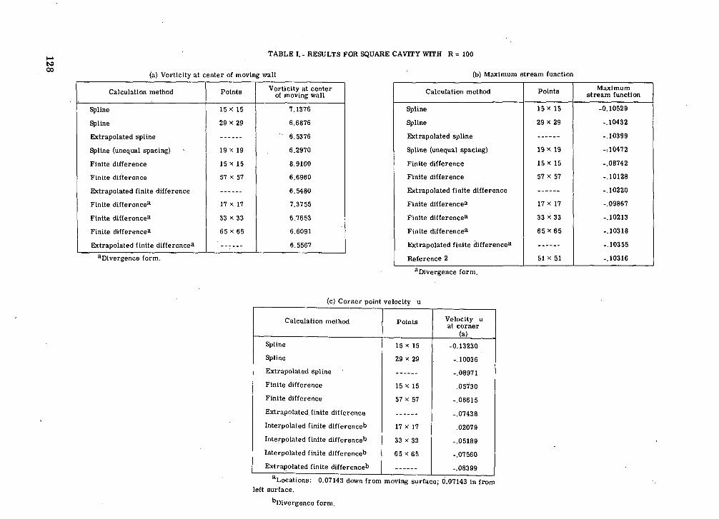
s3a£
co£
"0
§ait;CO
wco•a£SCo3CJ
73u
OJ
CM
O
)CM
C
O
OJ
tn
-^ eo
o
o
o
0
I
i
in
os•-t
CM
X
Xin
oj
rH
CM
0C"o,wT3CD
30
CU Q
J 5*
& & S
NS1OJXOS
ft
'Soc1ssr1
CMC-
ao'
inXinCJ
ccucu0)
c
ooCM0
1
r-mXt-CDCJS<u'•3cE
0g1C0)VCU
"cCUrt"oc1
t-coooOJ1
c-Xt-%cCU
IH3c£
CO
CM
O
1
CO
COXCOCO
rtoc0)
IH
•3CD
C
CO
s1
mCOXinCDrtucCUt-.QJCUC
inCOo
1CUcQJCD
"cQJ
_rt"oi
CD
COO
1
1-tinX^H
CMCJ
gI
g^
CJ
^
rt C
^- o
0*0COcIoCUco"rt
"3CJ
s
CO
CD
CDt-
c-
t-CO
O
O
CO^H
C
D
int-
CD
C
O
<-i C
M
X
Xm
en
.-<
CM
OSc"a.COrt
"oIX<U
CU rt
£.
£*
•*
W
t«
W
0c~CMCDoXOS
"Si
g'ort
1a*CUc•f.s1
oCO
OJ
00inX2CUcCD(HCD
-a0)c
0CDCO
CD
t-tnX[-u
teren
TJ0)C
O00
CDCUCJcCDitCD
'c•oCD"rtai
ininr-cot-c-Xt-rtCDCJ
cCUCD
"O0)c
sCDc-CDCOCOXCO
CO
rtScCD
TJC
OJ
oCDCDinCOXinCDrtCDUCCUftCDC
c-CDininCOrtCDucCUItCD
"cCDrt
1rt .
1
goCDCJ
CSH°
CD
Qrt
3>»
°
'o o «O
O
s, rt
•2cop.1tu1
Calculal
O
CD
1-1
CO
C
O
t-CNJ
O
OS
CO
O
C
O*-(
I-H
O
o i"
«'1
m
oji-H
CM
X
Xm
o»
i-H CM
CDC§••o<us"o£
« S*
S S
^"3.
Q.
"SW
C
O
W
0•5oinrHXmCUC
JcCU
'•B'cfa
sCDCD0r'
t-inXt-inCUC
Jc2CD
'DCUcfa
COCOr-0rCOQJf*
•n0)
'crtrapolated
W
OS
c-oCMOc-1-4
XXICDCJC<0ItCU
!tiCD
'cterpolated f
c
OJ
ooinoi"
COCOXCOCO
xsCUcCU(HCD
!t*CU
"sterpolated fc
oc-orCDXmCD
XICDCJcCDIH
«"OCD
"c:erpolated fc
OJ
COCOol"
"%CDttCD
*nCDCrtrapolated :
w
a2cCOt-OOCJ
S.
foI**-•c"OCOPH
.
ooaLocations:irface.«CD
128
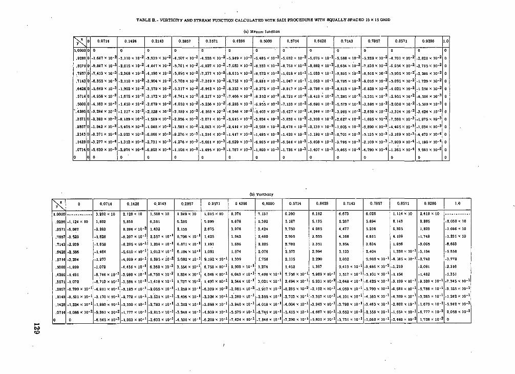
i8I !
HuIa>.ia
o~4
iOS
O§o
0.7857
St-0CMSo*c-os0
0.4286
toOinso
0.2143
ca2o
0.0714
uo0ooo0ooo0oo—•
°CMXCMC?
caoXot^7CMOXcaCMin0XCOin
ca0XCDCD"?
caoXin
CMoXin•«•in
CMOOS
V"?CMOXC
O
cnTcaoXs^"?XOS
eooseo
caoXoCO
CMOXi7o>
°egXmt-LVCMOXso"?CMOXO)
eo*70XeoCO
CO*
CM0.
Xcs-O
O
CO
caoX°?CMOXeoeo*caoXtoCD
t-
CMOXe-coCDOXcoU. J
CMXf-
TcaOXCO
CM
co0XI—O
S
e-co
caXCDS"CMOXoOS
"/
CMOXininCO
.0
-9.865 x
oXtoo7oXCO
0CMOXCMinOS
oXcoCO
CMOXKr-
egOXinOS
CO
ufCMX2•V
CMOXsCO
to0XCO
Ve-eoc-
caXOS
cat-
CMOXos
OuioXCD
0CO
0Xino>t-e»0Xso>H
OXSCMOXOS
oXsCO
CMoXOS
st-
ca0X="r
caxsOS
1CMOXoCM
eo0XinCO
ieot-
CJXsca7caOX§rcaOxCO
3CO0XCO
eoCO*
ca0Xst-cn
CMOXosOS
egOXcatoOS
0XtoeoCO
CMOXCMSCD
egoXr-tout
caXOS
eo
CMOXsOS
*7
eoOXOS
sinCMCO
COxSCMOXus
OS
CVOXintoin
CMOXCOCMr-"
CM0
' XoV°?CMOXCM°?
CMOXCMeoCO
OXCOCO^*r-
caoXt-egCD
CMoXi?7caXCMco
caoXint-CD
•7COoXCD
OS
^V
eoXioxos*•?oXcneoeo
CMO
-5.573 x
CMOXSCD"?
caoxCO
eo
TOXoCO
0XeocaCD
caoXsCM"?
CMOXooTcaXCOCD
CM
caoxo•*7eooXCO
CD
11
coX|*iox7oXgCDCM
ego
-3.965 x
CMQXIVCMOXf'CMmoxCO«. «
ft
•CM0X<DS^«
raOXCOco7CMOXOS
CO
"?caXCO
ca
ca0Xt^7COoXi•?tos/
COXi7tooXCO
OS
*7CMOXinC
OC
O-7CMOxCO
CM
CMOXcacneoCO
caoXoeo
CM0X•crCO
CO
CMOXinto"oXs°?CMOXtoin
CMX17eoOXcneo
eoOXiCMKco
COXeoO7to0XintoTeoOXSOS
egoxtooto
caoXo>eoca
CMOXCO
ca
CM0XCOin"?CMOxs•Veg
caoXiNegoxCO
s7CMXCO
s7tooXs*?eooXcaS7C
OCM
*tXto•V"TeoOXOS
CD
*vtoOXtneoincooXoCO*
oxCOOS
7ca0XoCM7ca0Xinv7CMOx£V7caOXsca7eoOXCD
SeoXto
eooXs0CO
*foX•?eo?H
CM
°T
XI70XOSoo>
eoOXOSo"?eoOXO
S
cooXCOoin0XstooXtncnC
D
tooXOS
CMtoCD
tooXCDtotn
iOXCO
sTeo0XtoCM
COoXca7voXS•7CO
•<r
°COXCO
cnoX
- CDeo
7OXSt-To
-9.465 x
oXs70Xtoeo
eoOX000
7eoOXtoe-7COoXinO
S
7tooXCOo7•O
1xeoS"?0XIegtnOX8int-o
°0ooo0oooo0o
01OS
ot-eooso
0.7143
to0ino0ioKtoOKCO
CM
OeoOCMOioo
2.419 x 1
x1-1
cogCO
eoCO
CO
CMcnCDgCDCO
r-coCOoXinortXen**oX~X§xCM§§**
XosCD
00
O>
eo00
1inCDCMmwinitocacoCOCDO
S
ostnCM
CDCO
CDeoCO
CMCOOX78S
X
XS
«
eo
CD
co co
in
to C
M
co co
CO ?
O
^-*'
— i
co to"
Xin
cn
co
eo
0
0
m e
oco
•-« co
eo
CO
~
M1
M1
s s
s s
m
v eo C
M
£
S
S S
3v
v
co
eo
co in
m
o>
V
eo eo
pa
Stft
eg co
OS C
O
l-r»
os
t- m
co C
M
N
. pa
v
O
m
toca
to
N
t-
co pa
to
f
S-
g-
o>
t-
3s co
m
in
m
-i I-H
t- C
M
cn os
CD •*
~
0CM
-H
-*
^H
XX
Xin
o
«
vin
os
r- co
^H
t- C
O
-«
CM
CO
CD
CO
O
O
O
XX
XCM
C
~
if 1 C
MO
f»
O
— i
-
CM
~
-
x x
x x
S
o
S
Sos
co C
D
tn
to
co
S
,rC
M
CO
C
D
V
CO '
CM
C
O
CO
o
tn
os
tnin
co C
M C
M
?
K
5
Stn
co
—
^r
eo t-
t- to
t-egXinSoXcnosOS
ipaSCMpatnCMoseoCOoXcaOS
OSXomCMOXisCO'X1*vf-CN
i«?to
toeoat
0CM*
OeooXCO
CO
eo
-7Xeo
cnasto-*tn"s7
XOS
oXr-CD•Xinineo
ioXcnCD
CO'Xto"TasOi78S
inCOCMto5oxo"?-7Xt--*oXcnOS
tn
7
Xse-t-oXCO
OS
*7xcoSoXCD
O-r.xi~oXstoXOS
*Y7xVcn7CD
CM
*7X7xoscn•X1os
OXmCD
7XosCDC
M
OXtoOS
in
7XvOJ
oxs7x•*»•oXSs
-1xp—oX•7•Xiv{7
Xo. e
-
C4
o-7tnco
*7xmCM
7xto.Xs*?oXOS
OS
*?-7Xso7oXCMOS
P4
egx"?ot-7*?XCOo
caOxOS
eoCD•XS70Xin"7XinCO
vt
7XCOoXt-«?inCO
pa
7
xcaca
7
XeoSco'
•XSeoToxeoST-7xoToXinCO
eo
7
Xtot—°?oxineoc?
•7xcnCD*}OXegpa•xCO
sCMOXca«?•Xr-c?
7Xo-*0X•7coCM
*?Xpacn
7xt-co.X1*?oxeotoCO
7
Xt-*?oXeocnco
7
XToxOS
o7*7Xo*?oxCOO)
to7XCM
CM"7oXeoCO
CM'XoeoeoL?
*7xCO0X-71
*?x0°?Xt-t-toiXin•7oxsinCM
paXCD
*?OXiT7XininOX*V7
579 x 1
oXcncnT•XCO
cnCOoxpa'Xi-f~'!CMXCO0X•7o
°?X§caXCOoXcnS77
731 x 1
*?0XoCOin7
X1«7oxtos1T7x5ToXCD•X7oeoeoCM'Xeo§'.'
eoXino0
129
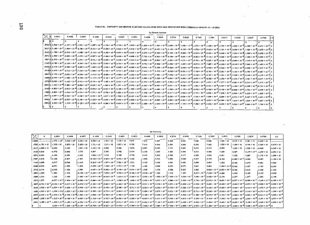
-sor-o>or-05
Ot-r-ooSo"
oosCPo'
o*0oSoiso0o
X
o
oo?0
«=1s
o
—aio
—Ioioi
o
— '
oI0
-
MO10 7•.C
4
O
0
§ss°CO
0s3CD
osO
10
<=>
02?",'o-.osSoI•7oisO5ooTfj^r-ZCO
CO
2i2CD
•iiCO
aoig!1
o
o
S
S
«
M
2
2
S
n
S
s
o
ce
2
2
§ s
to t>
J
S
o
o
i I
«
g
co' CD*
o
o
I 1
CO
C
O
CN
M
0
0
S
S
q-
g
to
d
O
O
r- o
2
2
•r T
—
CO
S
S
o
o
2
S
o
o
g 1
"•I
0szsgt-2«?
C0
AOooa1O)
INOg5OSO9
sin':2<N
OiS
o
o
to
™
"7 7
2
2
1 1
.310* 10-
.702 X 10-
g a
2
2
S
ST
•?
£ S
O
O
i 1
CO
O
S
O
CO
o
o
s s
O>
O
S
d
CN
o
o
s ;
f °?1 1
1 i
a 2
S
g
o
o
i i
*?" *?
to o
5
B'
o
o
S i
o
o
!!t~ c0
0
0
E
S
•? T
2
2
i 1
S
S
— : —
-
1 i
2
2
2
S
-T-fT
S
5
o
o
S
r-
S
oC
O
[-'
3
2
S
Xeo
co
(M
IN
o
e>
i s
2
n
2
3
? 1
T'
":
O
O
S
S
1 ;
i i
T. "J
2
2
7
O
° a
" 3
T *?
i§
o
o
£
PM
_,
2
2
^s.
05
«
-TT
-^-
s t
S
g
2
2
o
o
« C
O
CO
«
•* co
2
2
8 I
in
c^
W
M
0
0
S
£
—
O
2
2
5 2
o
o
5 i
t=>
0
•7 «?
S
P
o
o
1 S
o
o
§!
! 1
o
o
. ~
2
2
S S
T 7
-4.307 x 10
-2.100 x 10
2
2
S
g09
•«
•
S
?
o
o
o
o
(0
O>
§ 1
«? 7
CN
«
O
O
S
S
i 1
o
o
—
O)
5
2
0
0
IN
—
3
S7
°?
s y
5? S
o
o
CB
C
O
O
O
« s.
S
2
o
o
2
2
3 1
s **
': ':
i i
S
gO
IN
0
S
a
o
1 g
S. §
CD
M
1 2
»
CJ
n
no
o
S
S
S
2
o
o
«
to
0
0
•»
t-
a s
o
o
3 S
o
o
i i
i. 1.
o
o
S
X
" "
2
2
s i
— S
T
f
I i
T
T
2
2
i i
3
ST
T
o
o
—
O)
T
T
M1 s
<? 7
o
o
P
S?
7
1 S
o
o
S
S
o
o
s i
3 1
s s.
s °
CO
IN
IN
—
«?
To
o
s s
1 1
000aooo0oo
S
SS
a> to
o
o_
5
5
™ 2
s sS
S
S
g
r: SS
2
SiB
si3
il.
7 7
7 ~
, 7
•? -72
2
S S
2
2
2
s s i g
I i
s
I i 1
i i
B I ;
S 1
s s i s
i 1
S
s ? a = s s
|g
|g
|g
2X
to" «i
N
tf c-'
»
u> r>'
T' T
S ; s
s s s g
"•*'•!•:
S
g
130
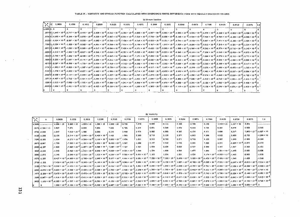
i I
u
IO
J!
O.
£ost-«too1tooss—
0.5000
PCO0toin0S002CO
o'
008o'
"*./
ooooo0oooo0I—
0Ol•0s~C
M~
0o>
CMOtoD
O
CO
CM0Xs0sfMr-
Ol
CMOCO0offi
0(O
7T~
0xOl
1*?to
*?or-t-=or-
0Si0CO
~C
M~0t-
CM0COCO
CM0XCOCO*
0OCO
oCM0r-'
0CD
CO
0r-
~C
M~
0Xs**COCO
«MsiossCO
00
0
01
in
v«
00
0
—
in
t-
CM
CM
CM
00
0
S
S
S
CM
O
) C
M
00
0
S
2
£
Ol
Ol
Ol
CM
—
~
00
0
? 1 i
00
0
in
«
00
ci —
01
co co
ino
m
,*
0>
0>
e»
CM
CM
CM
00
0
sis
co'
co
co
00
0
§ § !•0
O
0
0
01
CO
"5 —
M IM
00
0
S
S
3"
T T
ill
CO
S
»
CM
C
M
CM
00
0
1 i
s
00
0
co in
«
eo m
oo
sis
eo r-
to
1P°7i~oCM0sCO*
CM0o0s"eT
~
COCO
CM0oco'
0t-gto"
0Ol
"iM~0CM
•*
SCM21oC
4C
O
OE:i2
-5-ogC
M=>
i
-7.236 x 1
CM01o0COCO
sCOt-'
CM0t-01CO0n3-~0p*i5N-3i|i
0
0
<o
m
o
o
S
S
CS
. C
M
O
O
o> o
o
—,
CM
CM
2
2
1 1
? |
CM
CM
0
0
SI
o
o
o> in
„ „
to' 10
CM
CM
0
0
Ol
CM
o
o
1 ;•0
0
W
Ol
M
w
0
0
CM
tO
CO
CM
—
t-
CM
eo
2
S
! 1o
o
CM
S
~o
— in
o
to
m
o
o
o
o
to
CM
C
M
o
to
s z
CM
M
§ i
eo C
M
CM
CM
o
to
ES
0
O
i i
0
S
CM
C-J
0
0
S
2
0
0
g 1
CM
OJ
0
0
o
oj
•? s
^
M'
0
0
0
?
*? 7
1 1
t- t-
eo C
O
2
2
1 i
O
O
to
i-
s s
tot-0«to1COoO
**?iCMOt>toOl
"c5~~
Ol
co
CMOO
>
toinSO&
"c?~OtoOl
seo-™
-
Oioo
oOl
os~eo~0CO02"aeo•=>-9.208X
0o
~C
M~
iCM0o0C
Ooto
~rT
~
oOl
1/5seofat-0to«
inO?IS
~co~0Seo0g*?seo0flCO0111CO0O
l
CO0§0§~n~
0K«'•'g•V-ir-'
0COmCM
0"inot-to
~^T
~
0g^>°s'
CO
*00mCO0s~n~
CO8.(00o>oCO0CO
0CO
__
_
0Utot-
f-ioi-55-i
0o0oooo00o
CM
eo
Sr
^c
oc
Mi
nS
—
S
eo
eo
cM
cM
io
in
oc
BC
MC
MO
ir
-
g 8 S i £
OOOOOOO
i I s 1 ? S 1 =«
-• «• ^ «
_• vO
O
O
O
O
O
OO
OO
OO
O
00
/0
S«
V
eo
01
to
mS
=
S
00
0
X
X
o
o
0
o
o
OO
OO
OO
O
o
r- to — o
t- c*i
to o o o o o
v x
x y
x x
s s
s
00
0
X
X
X
X
7
O
m
CO
C
M
O
O
O
x x
y
OO
OO
OO
O
y x
x x
x v
xC>4
CM
O
C
D
«
OO
to
2
E
S
g
8S
2
00
00
00
00
00
00
00
2 2
y x
ooooooooooo
00
00
0
«c
or
-t
ot
ai
nc
nv
2
2
§
131
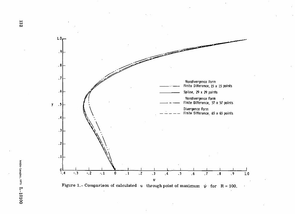
a a
Lo
ooI—I
IItiSc.*—i
oo.
f(-1
TJ0)
13U§ra'CrtIoO
132N
ASA
-Langley, 1975 L
-10100
NATIONAL AERONAUTICS AND SPACE ADMINISTRATION
WASHINGTON. D.C. 2O546
OFFICIAL BUSINESSPENALTY FOR PRIVATE USE $3OO SPECIAL FOURTH-CLASS RATE
BOOK
POSTAGE AND FEES PAID
NATIONAL AERONAUTICS AND
SPACE ADMINISTRATION
491
071 001 C1 U A 751114 S00903DSDEPT OF THE AIR FORCEAF WEAPONS LABORATORYATTN: TECHNICAL LXBRft-HY-KIRTLANU AFB MM 871. 7
POSTMASTER : If Undeliverable (Section 15SPostal Manual) Do NotRetui
"The aeronautical and space activities of the United States shall beconducted so as to contribute . . . to the expansion of human knowl-edge, x>f phenomena in the atmosphere and space. The Administrationshall-prayide for the widest practicable and appropriate disseminationoj •in.jptmdiioit concerning its activities and the results thereof."
• I ; . •• v' ^NAtj'oNAL .AERONAUTICS AND SPACE ACT OF 1958
NASA SCIENTIFIC AND TCEGHNi€AL PUBLICATIONSTECHNICAL REPORTS: Scientific andtechnical information considered important,complete, and a lasting contribution to existingknowledge./•<,.. "•' /•..
TECHNICAL NOTES Information less Bro^dj,in scope but nevertheless of importance as acontribution to existing knowledge.
TECHNICAL MEMORANDUMS:Information receiving limited- distributionbecause of preliminary data, security classifica-tion, or other reasons. Also includes conferenceproceedings with either limited or unlimiteddistribution. • .
CONTRACTOR REPORTS: Scientific andtechnical information generated under a NASAcontract or grant and'considered an importantcontribution to existing knowledge.
TECHNICAL .TRANSLATIONS:; Informationpublished in a foreign language consideredto merit NASA distribution in English.
SPECIAL PUBLICATIONS: Information•derived from or of value to NASA activities.Publications include final reports of majorprojects, monographs,.data compilations,handbooks, sourcebooks, and specialbibliographies.
TECHNOLOGY UTILIZATIONPUBLICATIONS: Information on technologyused by NASA that may be of particularinterest in commercial and other non-aerospaceapplications. Publications include Tech Briefs,Technology Utilization Reports andTechnology Surveys.
Details on fhe availability of fhese publications may be obtained from:
SCIENTIFIC AND TECHNICAL INFORMATION OFFICE
NATIONAL A E R O N A U T I C S A N D S P A C E A D M I N I S T R A T I O N
Washington, D.C. 20546