1

Independence and Conditional Independence in Causal Systems

Karim Chalak and Halbert White1

Department of Economics

University of California, San Diego

May 5, 2007

Abstract: This paper studies the interrelations between independence or conditional

independence and causal relations, defined in terms of functional dependence, that hold

among variables of interest within the settable system framework of White and Chalak.

We provide formal conditions ensuring the validity of Reichenbach’s principle of

common cause and introduce a new conditional counterpart, the conditional Reichenbach

principle of common cause. We then provide necessary and sufficient causal conditions

for probabilistic dependence and conditional dependence among certain random vectors

in settable systems. Immediate corollaries of these results constitute causal conditions

sufficient to ensure independence or conditional independence among random vectors in

settable systems. We demonstrate how our results relate to and generalize results in the

artificial intelligence literature, particularly results concerning d-separation.

Keywords: Causation, Conditional Exogeneity, d-Separation, Reichenbach’s Principle,

Settable Systems, Structural Equations

Acknowledgment: The authors thank Julian Betts, Graham Elliott, Clive Granger, Mark

Machina, Dimitris Politis, and especially Ruth Williams for their helpful comments and

suggestions. All errors and omissions are the authors’ responsibility.

1 Karim Chalak, Department of Economics 0534, University of California, 9500 Gilman Drive, La Jolla,

CA 92093-0534, kchalak@ucsd.edu, http://dss.ucsd.edu/~kchalak

Halbert White, Department of Economics 0508, University of California, 9500 Gilman Drive, La Jolla,

CA 92093-0508, hwhite@ucsd.edu, http://weber.ucsd.edu/~mbacci/white

2

1. Introduction

The concepts of independence and conditional independence are central to many

disciplines, including probability theory, statistics, econometrics, and artificial

intelligence (see e.g Granger, 1969; Dawid, 1979, 1980; Florens, Mouchart, and Rolin

1990; Studeny 1993; Chalak and White, 2006). In particular, they are concepts central to

the study of causal inference (see, e.g., Rubin 1974; Holland, 1986; Spirtes, Glymour,

and Scheines, 1993 (SGS); Pearl 1988, 1993, 1995, 2000; Dawid, 2000, 2002;

Rosenbaum, 2002). In this paper, we study the interrelations between independence or

conditional independence and causal relations, defined in terms of functional dependence,

that may hold among variables of interest within the settable system framework of White

and Chalak (2006) (WC), a formal mathematical framework for defining, identifying,

modeling, and estimating causal effects.

The interrelations between conditional independence and causal relations have been

extensively studied in the artificial intelligence literature. This literature introduced

graphical algorithms applicable to directed acyclic graphs (DAG) to characterize

independence and conditional independence among variables in “Bayesian Networks” or

more specifically “directed Markov fields.” In particular, our results relate to notions of

“d-separation” (Verma and Pearl, 1988; Geiger, Verma, and Pearl, 1990; Geiger and

Pearl, 1993; Pearl, 2000), “D-separation” (Geiger, Verma, and Pearl, 1990), and

alternative graphical criteria (Lauritzen and Spiegelhalter, 1988; Lauritzen, Dawid,

Larsen, and Leimer, 1990).

The topic of this paper is also central to certain strands of the philosophy literature

(Spohn, 1980; Hausman and Woodward, 1999; Cartwright, 2000). In particular,

Reichenbach (1956) introduced his “principle of common cause,” which states that if two

variables are associated (e.g., correlated) then either one causes the other or they both

share a third common cause. Although this principle has intuitive appeal and despite its

venerated status, its formal standing is nevertheless ambiguous. Is it an axiom or a

postulate, or is it a logical consequence of assumptions as yet unformulated? Here we

provide a formal proof of the Reichenbach principle of common cause. The framework

supporting this proof is that of WC’s canonical recursive partitioned settable systems. We

also introduce a new conditional counterpart to this principle that we term the conditional

Reichenbach principle of common cause. We then build on these results to provide

necessary and sufficient causal conditions for dependence and conditional dependence

among certain random vectors in settable systems. Immediate corollaries of these results

constitute causal conditions sufficient to ensure independence or conditional

independence among random vectors in settable systems. This has direct connections to

notions of d-separation and D-separation introduced in the artificial intelligence

literature.

Thus, our results contribute to answering two questions of interest for the study of

empirical relationships. First, what restrictions (if any) on the possible functionally

defined causal relationships holding between variables of interest follow from knowledge

3

of the probability distribution governing these variables? Conversely, what implications

for their probability distribution derive from knowledge of functionally defined causal

relationships between variables of interest?

This paper is organized as follows. In Section 2, we introduce a version of WC’s settable

system framework. Using this, we provide rigorous definitions of direct and indirect

causality based on functional dependence, relevant to the study of direct and indirect

causality in experimental and observational studies. Although graphical representation of

our definitions and related concepts is helpful to heuristic understanding, our analysis

does not rely on properties of graphs. Instead, the analysis is entirely standard, driven by

functional relationships holding among the various components of a given settable

system. We refine previous definitions of indirect causality to accommodate notions of

causality via a set of variables and exclusive of a set of variables in recursive systems,

extending notions introduced by Pearl (2001). Section 3 provides a proof of the

Reichenbach principle of common cause for recursive systems. We then provide

necessary and sufficient conditions for probabilistic dependence among random variables

in settable systems. In Section 4, we build on the results in Section 3 to introduce and

prove the conditional Reichenbach principle of common cause and provide necessary and

sufficient conditions for probabilistic conditional dependence of certain vectors of

random variables in settable systems. In Section 5, we discuss how our results relate to

and generalize results of the artificial intelligence literature related to d-separation and D-

separation. Section 6 concludes and discusses directions for future research. Formal

mathematical proofs are collected in the Mathematical Appendix.

2. Direct and Indirect Causality in Settable Systems

We work with the following version of WC’s definition of settable systems. We let ∞ ≡ × × … .

Definition 2.1: Settable System Let (Ω, F) be a measurable space. For h = 1, 2, … and j

= 1, 2, …, let settings Zh,j : Ω → be measurable functions. For h = 0 let setting Z0 : Ω

→ be a measurable surjective mapping. For h = 1, 2, …, and j = 1, 2, …, let response

functions rh,j : ∞ → be measurable functions.

For h = 1, 2, …, and j = 1, 2, …, let Z(h,j) be the vector including every setting except

Zh,j, and define the settable variables Xh,j : 0,1 × Ω →

Xh,j (1, . ) = Zh,j

Xh,j (0, . ) = rh,j (Z(h,j)).

For h = 0 let Xh (0, . ) = Xh (1,

. ) = Zh.

4

Put Zh ≡ Zh,j : j = 1, 2, … , Z ≡ Z0, Z1, …, rh ≡ rh,j , j = 1, 2, … , r ≡ rh , Xh

≡ Xh,j : j = 1, 2, … , and X ≡ X0, X1, ….

The pair S ≡ (Ω, F), (Z, r, X) is a settable system.

In Definition 2.1, we have a number of agents indexed by h responding to other agents in

the system. Each agent governs responses indexed by j. We denote the jth response of

agent h by Yh,j = Xh,j (0, . ). Thus, agent h’s jth response depends on the settings of all

other variables in the system, including not only the settings corresponding to other

agents but also those corresponding to agent h other than j. We refer to Xh,j as a “settable”

or “causal” variable. A settable variable has a dual aspect: Xh,j (1, . ) is a setting, whereas

Xh,j (0, . ) is a response. As we discuss shortly, we define causality in terms of settable

variables rather than random variables or events.

The setting Z0 plays a special role as a fundamental variable, that is, a variable that does

not respond to any other variable in the system, apart from its dependence on ω ∈ Ω.

This motivates the convention that X0 (0, . ) = X0 (1,

. ) = Z0. Indeed, we can identify Z0(ω)

with ω, as there is no loss of generality in choosing Ω = and letting Z0 be the

(measurable and surjective) identity map, Z0(ω) = ω. WC’s definition explicitly

accommodates attributes; for conciseness and without essential loss of generality, we

suppress these here. Thus a settable system S ≡ (Ω, F), (Z, r, X) is composed of a

stochastic component: the measurable space (Ω, F) and a causal structure: the settings,

responses, and settable variables (Z, r, X). WC and White (2007) discuss in detail the

relationship of the settable system framework to Rubin’s treatment effects framework as

formalized in Holland (1986) and to Pearl’s causal model (Pearl, 2000).

It is useful to partition the system under study to group certain variables into specific

blocks. WC and White (2007) discuss a number of examples where it is appropriate to

treat the system under study at the level of a certain partition but not another.

Definition 2.2: Partitioned Settable System Let (Ω, F) and Z be as in Definition 2.1.

Suppose that settings of X are given by Xh,j (1, . ) = Zh,j, h = 1, 2,…; j = 1, 2, …, and by

Xh (1, . ) = Zh for h = 0. Let Π = Πb be a partition of the ordered pairs (h, j): h = 1, 2,

… ; j = 1, 2, …. Suppose there exists a countable sequence of measurable functions rΠ

≡ r ,h j

Π : ∞ → such that for all (h, j) in Πb the responses Yh,j = Xh,j (0,

. ) are jointly

determined as

Yh,j = r ,h j

Π ( Z(b ) ) , b = 1, 2, …,

5

where Z(b) is the countable vector containing Z0 and Zi,k, (i, k) ∉ Πb. Then we say that rΠ

is adapted to Π. The pair S ≡ (Ω, F), (Z, Π, rΠ , X) is a partitioned settable system.

Settable systems provide a suitable framework for the study of causality. We next give a

definition of direct causality within this framework, based on functional dependence. For

this, we let z(b)(h,j) be the vector containing all elements of z(b) except zh,j.

Definition 2.3: Direct Causality Let S ≡ (Ω, F), (Z, Π, rΠ , X) be a partitioned

settable system. For given positive integer b, let (i, k) ∈ Πb. (i) If for given (h, j) ∉ Πb

the function zh,j → r ,i k

Π (z(b)) is constant in zh,j for every z(b)(h,j), then we say Xh,j does not

directly cause Xi,k in S and write Xh,j |d

S⇒ Xi,k. Otherwise, we say Xh,j directly causes Xi,k

in S and write Xh,j

d

S⇒ Xi,k. (ii) For (h, j), (i, k) ∈ Πb, Xh,j |d

S⇒ Xi,k .

In Definition 2.3, a settable variable Xh,j is said to directly cause Xi,k relative to the

system S if there exist some settings of all other variables in the system such that Xi,k

systematically responds to settings in Xh,j. Note that, by definition, variables within the

same block do not cause each other. In particular Xh,j |d

S⇒ Xh,j. Also, Definition 2.3

permits mutual causality, so that Xh,j

d

S⇒ Xi,k and Xi,k

d

S⇒ Xh,j without contradiction.

Mutual causality is ruled out in SGS (p. 42), for example, where it is an axiom that if A

causes B then B does not cause A. What we define here as “direct causality” is the notion

introduced in WC as simply “causality.” Here we require more refined definitions,

distinguishing in particular between direct and indirect causality.

We now introduce notions of paths, successors, predecessors, and intercessors, adapting

graph theoretic concepts discussed, for example, by Bang-Jensen and Gutin (2001) (BG).

Definition 2.4: Paths, Successors, Predecessors, and Intercessors Let S ≡ (Ω, F), (Z,

Π, rΠ , X) be a partitioned settable system. For given positive integer b let (i, k) ∈ Πb

and (h, j) ∉ Πb. We call the collection of settable variables Xh,j ,1 1,h jX , …, ,n nh jX , Xi,k

an (Xh,j, Xi,k)-walk of length n+1 if Xh,j

d

S⇒ 1 1,h jX

d

S⇒ …

d

S⇒ ,n nh jX

d

S⇒ Xi,k. When the

elements of an (Xh,j, Xi,k)-walk are distinct, we call it an (Xh,j, Xi,k)-path. We say Xh,j

d(S)-precedes Xi,k or Xi,k d(S)-succeeds Xh,j if there exists at least one (Xh,j, Xi,k)-path of

positive length. If Xh,j d(S)-precedes Xi,k, we call Xh,j a d(S)-predecessor of Xi,k, and we

call Xi,k a d(S)-successor of Xh,j. If Xh,j d(S)-precedes Xi,k and Xh,j d(S)-succeeds Xi,k , we

say Xh,j and Xi,k belong to an S-cycle. If Xh,j and Xi,k do not belong to an S-cycle, Xg,l

6

d(S)-succeeds Xh,j, and Xg,l d(S)-precedes Xi,k, we say Xg,l d(S)-intercedes Xh,j and Xi,k.

If Xg,l d(S)-intercedes Xh,j and Xi,k, we call Xg,l an (Xh,j, Xi,k) d(S)-intercessor. We denote

by ( )

( , ):( , )

d

h j i k

SI the set of (Xh,j, Xi,k) d(S)-intercessors.

Directed graphs can be used to illustrate a variety of aspects of settable systems. In

particular, they are helpful in visualizing the notions just introduced. For this, let G = (V,

E) be a directed graph with a non-empty finite set of vertices V = Xh,j : j = 1, …, Jh; h =

0, 1, …, H and a set of arcs E ⊂ V ×V of ordered pairs of distinct vertices such that an

arc (Xh,j, Xi,k) belongs to E if Xh,j

d

S⇒ Xi,k. From Definition 2.3, there exists at most one

(Xh,j, Xi,k) arc, and G thus does not contain “parallel arcs.” Since Xh,j |d

S⇒ Xh,j, there can

be no arc (Xh,j, Xh,j) in E, so G does not contain self directed arcs or “loops.” (Loops and

parallel arcs can nevertheless be useful in other contexts; see for example Golubitsky and

Stewart, 2006.) With loops and parallel arcs ruled out, a graph G associated with a

settable system S can be neither a “directed pseudograph” nor a “directed multigraph”

(see BG, p.4).

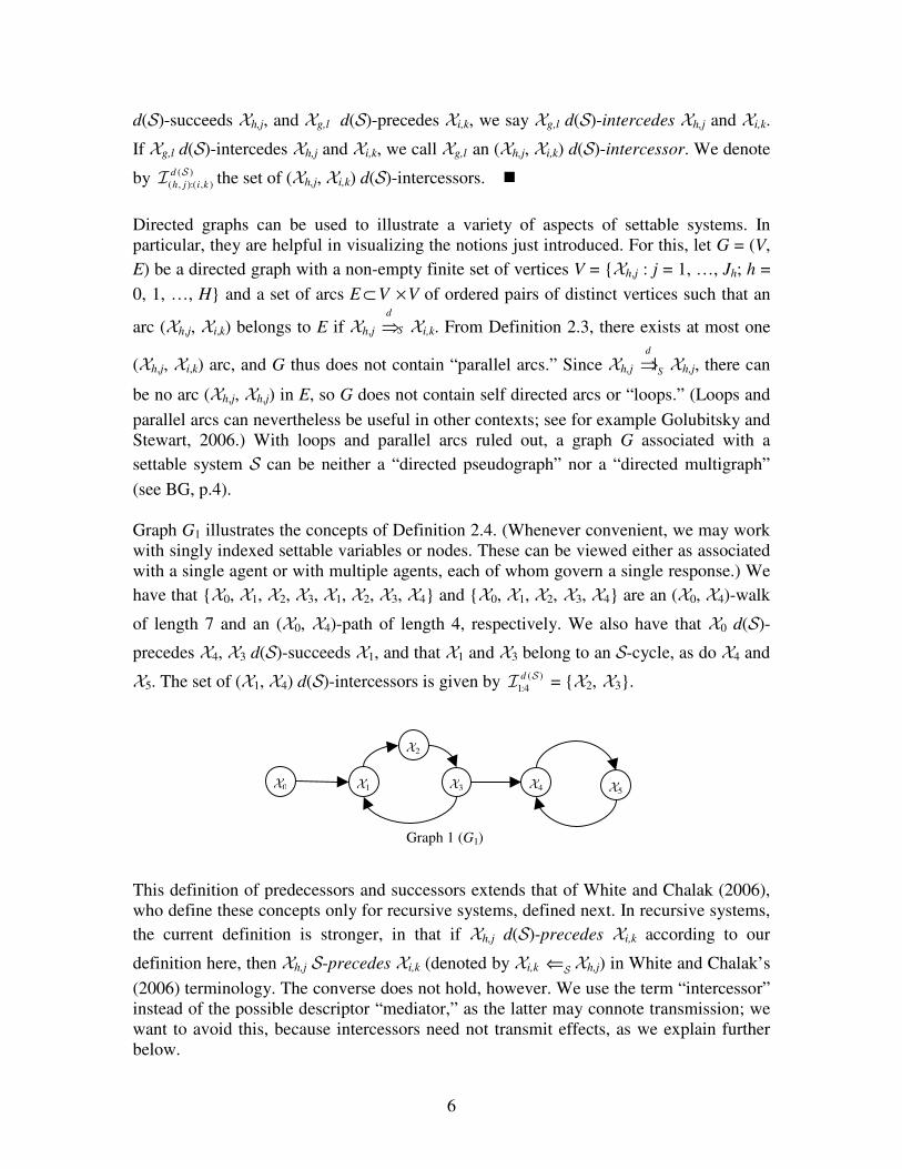
Graph G1 illustrates the concepts of Definition 2.4. (Whenever convenient, we may work

with singly indexed settable variables or nodes. These can be viewed either as associated

with a single agent or with multiple agents, each of whom govern a single response.) We

have that X0, X1, X2, X3, X1, X2, X3, X4 and X0, X1, X2, X3, X4 are an (X0, X4)-walk

of length 7 and an (X0, X4)-path of length 4, respectively. We also have that X0 d(S)-

precedes X4, X3 d(S)-succeeds X1, and that X1 and X3 belong to an S-cycle, as do X4 and

X5. The set of (X1, X4) d(S)-intercessors is given by ( )

1:4

d SI = X2, X3.

This definition of predecessors and successors extends that of White and Chalak (2006),

who define these concepts only for recursive systems, defined next. In recursive systems,

the current definition is stronger, in that if Xh,j d(S)-precedes Xi,k according to our

definition here, then Xh,j S-precedes Xi,k (denoted by Xi,k ⇐SXh,j) in White and Chalak’s

(2006) terminology. The converse does not hold, however. We use the term “intercessor”

instead of the possible descriptor “mediator,” as the latter may connote transmission; we

want to avoid this, because intercessors need not transmit effects, as we explain further

below.

Graph 1 (G1)

X3 X1

X2

X4 X0 X5

7

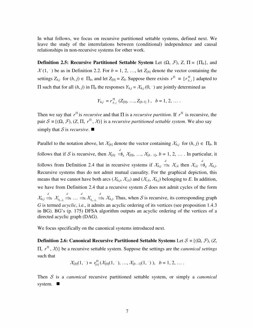
In what follows, we focus on recursive partitioned settable systems, defined next. We

leave the study of the interrelations between (conditional) independence and causal

relationships in non-recursive systems for other work.

Definition 2.5: Recursive Partitioned Settable System Let (Ω, F), Z, Π = Πb, and

X (1, . ) be as in Definition 2.2. For b = 1, 2, …, let Z[b] denote the vector containing the

settings Zh,j for (h, j) ∈ Πb, and let Z[0] = Z0. Suppose there exists rΠ ≡ r ,h j

Π adapted to

Π such that for all (h, j) in Πb the responses Yh,j = Xh,j (0, . ) are jointly determined as

Yh,j = r ,h j

Π (Z[0], …, Z[b-1] ) , b = 1, 2, … .

Then we say that rΠ is recursive and that Π is a recursive partition. If rΠ is recursive, the

pair S ≡ (Ω, F), (Z, Π, rΠ , X) is a recursive partitioned settable system. We also say

simply that S is recursive.

Parallel to the notation above, let X[b] denote the vector containing Xh,j for (h, j) ∈ Πb. It

follows that if S is recursive, then X[b] |d

S⇒ X[0], …, X[b - 1], b = 1, 2, … . In particular, it

follows from Definition 2.4 that in recursive systems if Xh,j d

S⇒ Xi,k then Xi,k |d

S⇒ Xh,j.

Recursive systems thus do not admit mutual causality. For the graphical depiction, this

means that we cannot have both arcs (Xh,j, Xi,k) and (Xi,k, Xh,j) belonging to E. In addition,

we have from Definition 2.4 that a recursive system S does not admit cycles of the form

Xh,j

d

S⇒ 1 1,h jX

d

S⇒ …

d

S⇒ ,n nh jX

d

S⇒ Xh,j. Thus, when S is recursive, its corresponding graph

G is termed acyclic, i.e., it admits an acyclic ordering of its vertices (see proposition 1.4.3

in BG). BG’s (p. 175) DFSA algorithm outputs an acyclic ordering of the vertices of a

directed acyclic graph (DAG).

We focus specifically on the canonical systems introduced next.

Definition 2.6: Canonical Recursive Partitioned Settable Systems Let S ≡ (Ω, F), (Z,

Π, rΠ , X) be a recursive settable system. Suppose the settings are the canonical settings

such that

X[b](1, . ) = [ ]br

Π (X[0](1, . ), …, X[b - 1](1,

. ) ), b = 1, 2, … .

Then S is a canonical recursive partitioned settable system, or simply a canonical

system.

8

In canonical systems, each setting Zh,j is determined as a response to its predecessors’

settings. These systems are particularly relevant in observational studies where control is

not feasible. When S is canonical, the setting and response values are determined entirely

by Z0 and rΠ . Thus in this case we also write S = (Ω, F), (Z0, Π, rΠ , X).

We next define notions of indirect causality in canonical systems. Pearl (2000, p. 165)

states that, “the notion of indirect causality has no intrinsic operational meaning apart

from providing a comparison between the direct and total effects.” Nevertheless, our

interest in the relations between causality and conditional dependence turns out to make it

natural to define several related notions of indirect causality as primitives, thus endowing

them with “intrinsic operational meaning.” We then relate notions of total causality to

those of direct and indirect causality.

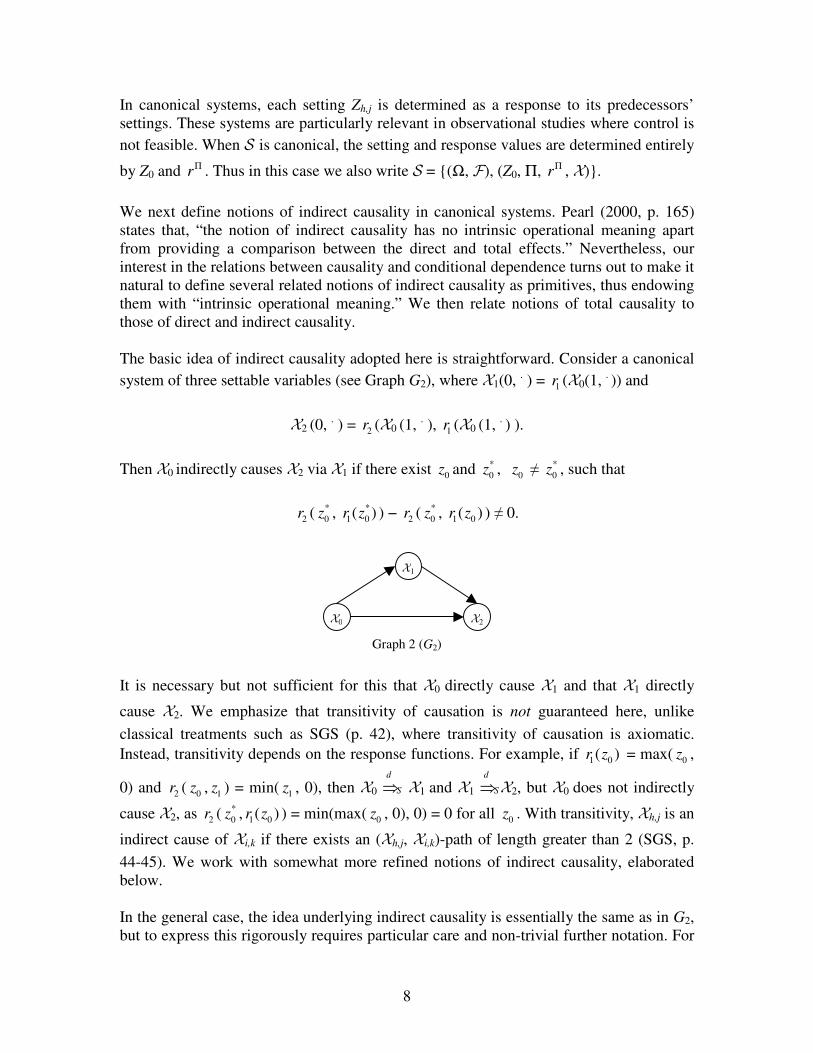
The basic idea of indirect causality adopted here is straightforward. Consider a canonical

system of three settable variables (see Graph G2), where X1(0, . ) = 1r (X0(1,

. )) and

X2 (0, . ) = 2r (X0 (1,

. ), 1r (X0 (1,

. ) ).

Then X0 indirectly causes X2 via X1 if there exist 0z and *

0z , 0z ≠ *

0z , such that

2r ( *

0z , *

1 0( )r z ) − 2r ( *

0z , 1 0( )r z ) ≠ 0.

It is necessary but not sufficient for this that X0 directly cause X1 and that X1 directly

cause X2. We emphasize that transitivity of causation is not guaranteed here, unlike

classical treatments such as SGS (p. 42), where transitivity of causation is axiomatic.

Instead, transitivity depends on the response functions. For example, if 1 0( )r z = max( 0z ,

0) and 2r ( 0z , 1z ) = min( 1z , 0), then X0

d

S⇒ X1 and X1

d

S⇒ X2, but X0 does not indirectly

cause X2, as 2r ( *

0z , 1 0( )r z ) = min(max( 0z , 0), 0) = 0 for all 0z . With transitivity, Xh,j is an

indirect cause of Xi,k if there exists an (Xh,j, Xi,k)-path of length greater than 2 (SGS, p.

44-45). We work with somewhat more refined notions of indirect causality, elaborated

below.

In the general case, the idea underlying indirect causality is essentially the same as in G2,

but to express this rigorously requires particular care and non-trivial further notation. For

Graph 2 (G2)

X1

X0 X2

9

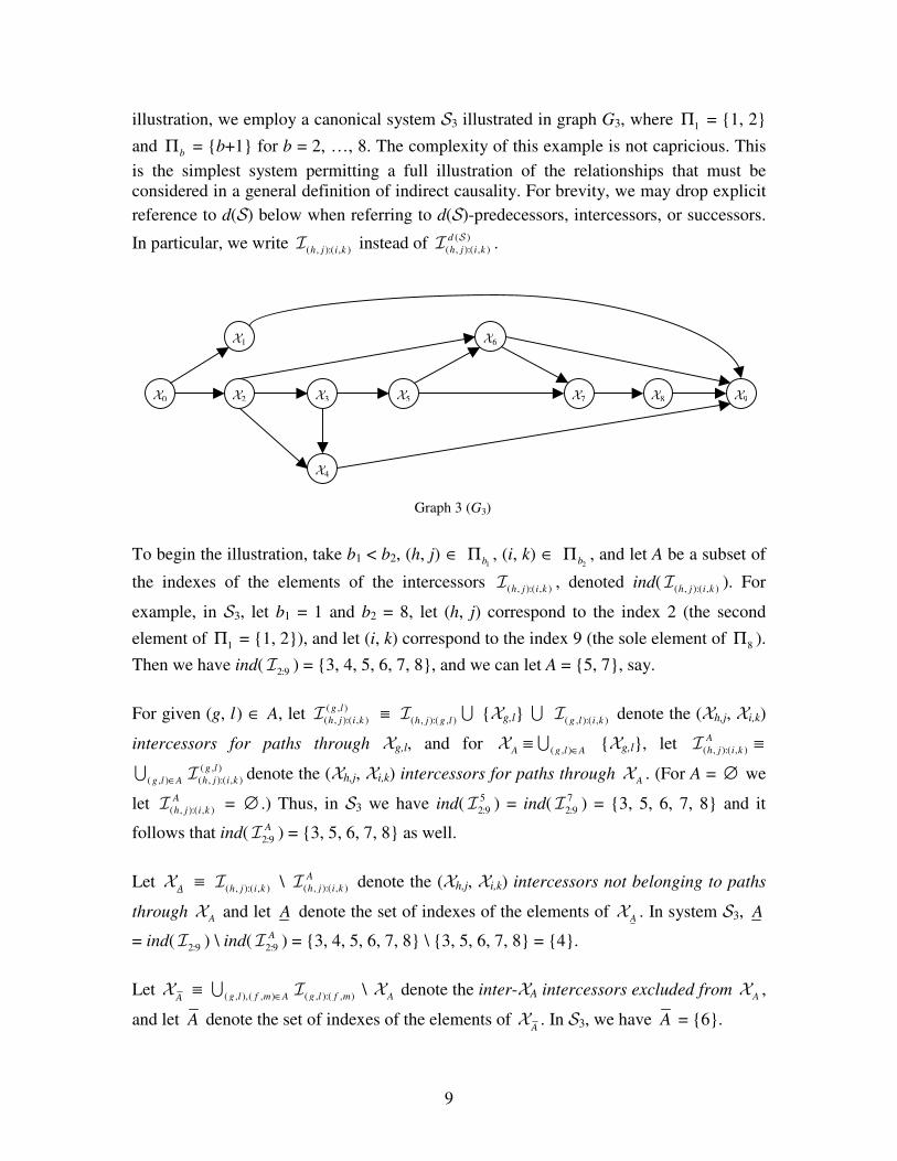
illustration, we employ a canonical system S3 illustrated in graph G3, where 1Π = 1, 2

and bΠ = b+1 for b = 2, …, 8. The complexity of this example is not capricious. This

is the simplest system permitting a full illustration of the relationships that must be

considered in a general definition of indirect causality. For brevity, we may drop explicit

reference to d(S) below when referring to d(S)-predecessors, intercessors, or successors.

In particular, we write ( , ):( , )h j i kI instead of ( )

( , ):( , )

d

h j i k

SI .

To begin the illustration, take b1 < b2, (h, j) ∈ 1bΠ , (i, k) ∈

2bΠ , and let A be a subset of

the indexes of the elements of the intercessors ( , ):( , )h j i kI , denoted ind( ( , ):( , )h j i kI ). For

example, in S3, let b1 = 1 and b2 = 8, let (h, j) correspond to the index 2 (the second

element of 1Π = 1, 2), and let (i, k) correspond to the index 9 (the sole element of 8Π ).

Then we have ind( 2:9I ) = 3, 4, 5, 6, 7, 8, and we can let A = 5, 7, say.

For given (g, l ) ∈ A, let ( , )

( , ):( , )

g l

h j i kI ≡ ( , ):( , )h j g lI ∪ Xg,l ∪ ( , ):( , )g l i kI denote the (Xh,j, Xi,k)

intercessors for paths through Xg,l, and for AX ≡ ( , )g l A∈∪ Xg,l, let ( , ):( , )

A

h j i kI ≡

( , )g l A∈∪( , )

( , ):( , )

g l

h j i kI denote the (Xh,j, Xi,k) intercessors for paths through AX . (For A = ∅ we

let ( , ):( , )

A

h j i kI = ∅ .) Thus, in S3 we have ind( 5

2:9I ) = ind( 7

2:9I ) = 3, 5, 6, 7, 8 and it

follows that ind( 2:9

AI ) = 3, 5, 6, 7, 8 as well.

Let AX ≡ ( , ):( , )h j i kI \ ( , ):( , )

A

h j i kI denote the (Xh,j, Xi,k) intercessors not belonging to paths

through AX and let A denote the set of indexes of the elements of

AX . In system S3, A

= ind( 2:9I ) \ ind( 2:9

AI ) = 3, 4, 5, 6, 7, 8 \ 3, 5, 6, 7, 8 = 4.

Let AX ≡ ( , ),( , )g l f m A∈∪ ( , ):( , )g l f mI \

AX denote the inter-XA intercessors excluded from

AX ,

and let A denote the set of indexes of the elements of AX . In S3, we have A = 6.

Graph 3 (G3)

X7 X5

X6

X9

X4

X3 X2 X8

X1

X0

10

Next, we distinguish between the (Xh,j, Xi,k) intercessors for paths through AX that

strictly precede or succeed XA.

We define the XA predecessors excluded from AX ∪

AX :

( , ):( , )

A

h j i kP ≡ ( , )g l A∈∪ Xf,m ∈ ( , ):( , )

A

h j i kI and Xf,m ∉ (AX ∪

AX ): Xf,m d(S)-precedes Xg,l,

and the XA successors excluded from AX ∪

AX :

( , ):( , )

A

h j i kS ≡ ( , )g l A∈∪ Xf,m ∈ ( , ):( , )

A

h j i kI and Xf,m ∉ (AX ∪

AX ): Xf,m d(S)-succeeds Xg,l.

In the example illustrated in G3, we have ind( 2:9

AP ) = 3 and ind( 2:9

AS ) = 8.

By construction, ( , ):( , )

A

h j i kI = ( , ):( , )

A

h j i kP ∪ AX ∪

AX ∪ ( , ):( , )

A

h j i kS , and ind( ( , ):( , )

A

h j i kI ) is a

subset of 1 2[ 1: 1]b b+ −Π , where for any blocks a, b, 0 ≤ a ≤ b, [ : ]a bΠ ≡ 1...

a b b−Π Π Π∪ ∪ ∪ .

We verify this equality in our example, where 2:9

AI = X3, X5, X6, X7, X8 and 2:9

AP ∪

AX

∪ AX ∪ 2:9

AS = X3 ∪ X5, X7 ∪ X6 ∪ X8. We write values of settings

corresponding to [ : ]a bΠ as z[a:b]. In particular, when (i, k) ∈ 2bΠ , we can express response

values for Xi,k as ,i krΠ (

2[0: 1]bz − ).

Next, let 1[0: ]( , )b h j

z denote a vector of values for settings for all elements corresponding to

1[0: ]bΠ except Xh,j. Thus, in S3, [0:1](2)z denotes values of settings for X0 and X1. Similarly,

let ( , ):h j Az ,

Az ,

Az ,

Az , and :( , )A i k

z denote vectors of values of settings for elements of

( , ):( , )

A

h j i kP , AX ,

AX ,

AX , and ( , ):( , )

A

h j i kS respectively. We treat elements of 2[0: 1]b −Π that do

not correspond to (Xh,j, Xi,k) intercessors as elements of 1[0: ]bΠ without loss of generality.

We now represent response values for Xi,k (recall (i,k) belongs to 2bΠ ) as

,( , )

,

A h j

i kr (1[0: ]( , )b h j

z , zh,j, ( , ):h j Az ,

Az ,

Az ,

Az , :( , )A i k

z ) ≡ ,i krΠ (

2[0: 1]bz − ).

The superscript notation A,(h,j) just introduced does not designate a partition but instead

acts to specify that the arguments of ,i krΠ have been permuted in a particular way, so as to

focus attention on settings of AX and Xh,j.

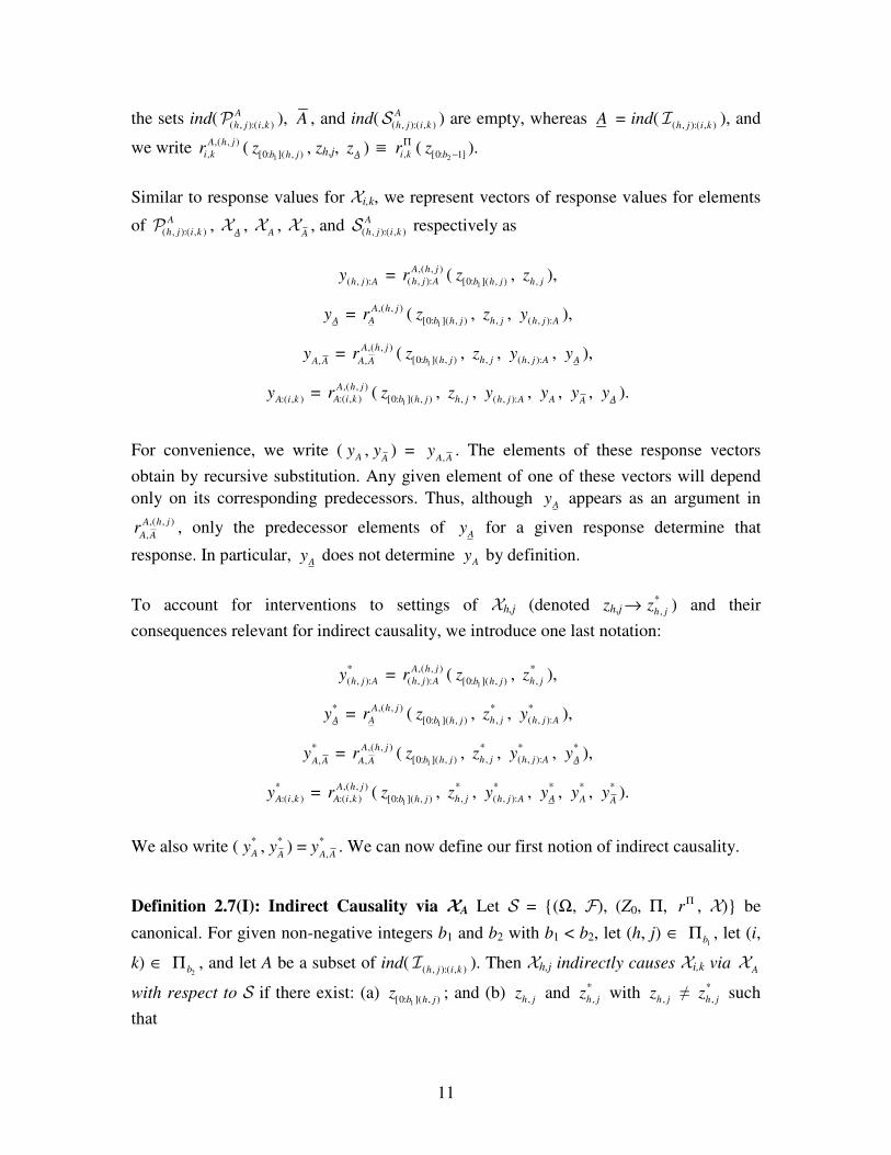
Observe that when A = ind( ( , ):( , )h j i kI ), the sets ind( ( , ):( , )

A

h j i kP ), A , A , and ind( ( , ):( , )

A

h j i kS ) are

empty and we write ,( , )

,

A h j

i kr (1[0: ]( , )b h j

z , zh,j, Az ) ≡ ,i kr

Π (2[0: 1]b

z − ). Alternatively, when A = ∅ ,

11

the sets ind( ( , ):( , )

A

h j i kP ), A , and ind( ( , ):( , )

A

h j i kS ) are empty, whereas A = ind( ( , ):( , )h j i kI ), and

we write ,( , )

,

A h j

i kr (1[0: ]( , )b h j

z , zh,j, Az ) ≡ ,i kr

Π (2[0: 1]b

z − ).

Similar to response values for Xi,k, we represent vectors of response values for elements

of ( , ):( , )

A

h j i kP , AX ,

AX ,

AX , and ( , ):( , )

A

h j i kS respectively as

( , ):h j Ay = ,( , )

( , ):

A h j

h j Ar (1[0: ]( , )b h j

z , ,h jz ),

Ay = ,( , )A h j

Ar (1[0: ]( , )b h j

z , ,h jz , ( , ):h j Ay ),

,A Ay = ,( , )

,

A h j

A Ar (

1[0: ]( , )b h jz , ,h jz , ( , ):h j A

y , A

y ),

:( , )A i ky = ,( , )

:( , )

A h j

A i kr (1[0: ]( , )b h j

z , ,h jz , ( , ):h j Ay ,

Ay ,

Ay ,

Ay ).

For convenience, we write (A

y ,A

y ) = ,A A

y . The elements of these response vectors

obtain by recursive substitution. Any given element of one of these vectors will depend

only on its corresponding predecessors. Thus, although A

y appears as an argument in

,( , )

,

A h j

A Ar , only the predecessor elements of

Ay for a given response determine that

response. In particular, A

y does not determine A

y by definition.

To account for interventions to settings of Xh,j (denoted zh,j →*

,h jz ) and their

consequences relevant for indirect causality, we introduce one last notation:

*

( , ):h j Ay = ,( , )

( , ):

A h j

h j Ar (1[0: ]( , )b h j

z , *

,h jz ),

*

Ay = ,( , )A h j

Ar (1[0: ]( , )b h j

z , *

,h jz , *

( , ):h j Ay ),

*

,A Ay = ,( , )

,

A h j

A Ar (

1[0: ]( , )b h jz , *

,h jz , *

( , ):h j Ay , *

Ay ),

*

:( , )A i ky = ,( , )

:( , )

A h j

A i kr (1[0: ]( , )b h j

z , *

,h jz , *

( , ):h j Ay , *

Ay , *

Ay , *

Ay ).

We also write ( *

Ay , *

Ay ) = *

,A Ay . We can now define our first notion of indirect causality.

Definition 2.7(I): Indirect Causality via XA Let S = (Ω, F), (Z0, Π, rΠ , X) be

canonical. For given non-negative integers b1 and b2 with b1 < b2, let (h, j) ∈ 1bΠ , let (i,

k) ∈ 2bΠ , and let A be a subset of ind( ( , ):( , )h j i kI ). Then Xh,j indirectly causes Xi,k via

AX

with respect to S if there exist: (a) 1[0: ]( , )b h j

z ; and (b) ,h jz and *

,h jz with ,h jz ≠ *

,h jz such

that

12

,( , )

,

A h j

i kr (1[0: ]( , )b h j

z , *

,h jz , *

( , ):h j Ay , *

Ay , *

Ay , *

Ay , *

:( , )A i ky )

− ,( , )

,

A h j

i kr (1[0: ]( , )b h j

z , *

,h jz , *

( , ):h j Ay , *

Ay , A

y , *

Ay , ,( , )

:( , )

A h j

A i kr (1[0: ]( , )b h j

z , *

,h jz , *

( , ):h j Ay , *

Ay , A

y , *

Ay ))

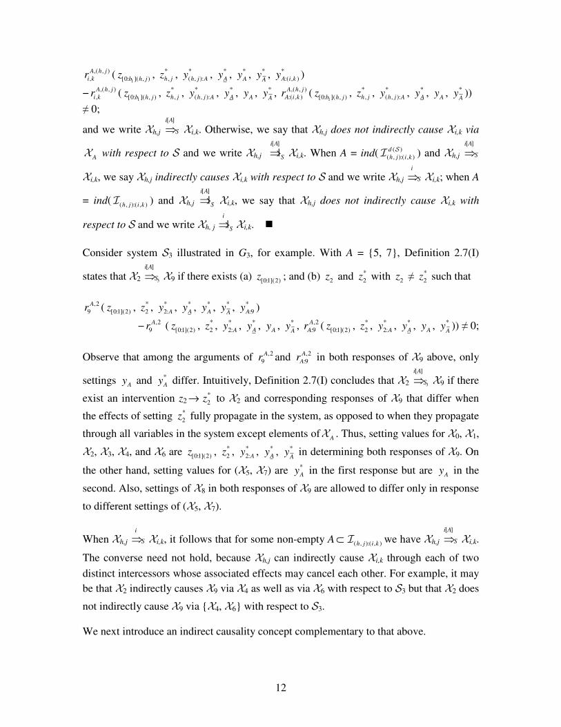
≠ 0;

and we write Xh,j [ ]

i A

S⇒ Xi,k. Otherwise, we say that Xh,j does not indirectly cause Xi,k via

AX with respect to S and we write Xh,j

[ ]

|i A

S⇒ Xi,k. When A = ind( ( )

( , ):( , )

d

h j i k

SI ) and Xh,j

[ ]

i A

S⇒

Xi,k, we say Xh,j indirectly causes Xi,k with respect to S and we write Xh,j

i

S⇒ Xi,k; when A

= ind( ( , ):( , )h j i kI ) and Xh,j [ ]

|i A

S⇒ Xi,k, we say that Xh,j does not indirectly cause Xi,k with

respect to S and we write Xh, j |i

S⇒ Xi,k.

Consider system S3 illustrated in G3, for example. With A = 5, 7, Definition 2.7(I)

states that X2 3

[ ]

i A

S⇒ X9 if there exists (a) [0:1](2)z ; and (b) 2z and *

2z with 2z ≠ *

2z such that

,2

9

Ar ( [0:1](2)z , *

2z , *

2:Ay , *

Ay , *

Ay , *

Ay , *

:9Ay )

− ,2

9

Ar ( [0:1](2)z , *

2z , *

2:Ay , *

Ay , A

y , *

Ay , ,2

:9

A

Ar ( [0:1](2)z , *

2z , *

2:Ay , *

Ay , A

y , *

Ay )) ≠ 0;

Observe that among the arguments of ,2

9

Ar and ,2

:9

A

Ar in both responses of X9 above, only

settings A

y and *

Ay differ. Intuitively, Definition 2.7(I) concludes that X2 3

[ ]

i A

S⇒ X9 if there

exist an intervention z2 → *

2z to X2 and corresponding responses of X9 that differ when

the effects of setting *

2z fully propagate in the system, as opposed to when they propagate

through all variables in the system except elements ofAX . Thus, setting values for X0, X1,

X2, X3, X4, and X6 are [0:1](2)z , *

2z , *

2:Ay , *

Ay , *

Ay in determining both responses of X9. On

the other hand, setting values for (X5, X7) are *

Ay in the first response but are

Ay in the

second. Also, settings of X8 in both responses of X9 are allowed to differ only in response

to different settings of (X5, X7).

When Xh,j

i

S⇒ Xi,k, it follows that for some non-empty A ⊂ ( , ):( , )h j i kI we have Xh,j [ ]

i A

S⇒ Xi,k.

The converse need not hold, because Xh,j can indirectly cause Xi,k through each of two

distinct intercessors whose associated effects may cancel each other. For example, it may

be that X2 indirectly causes X9 via X4 as well as via X6 with respect to S3 but that X2 does

not indirectly cause X9 via X4, X6 with respect to S3.

We next introduce an indirect causality concept complementary to that above.

13

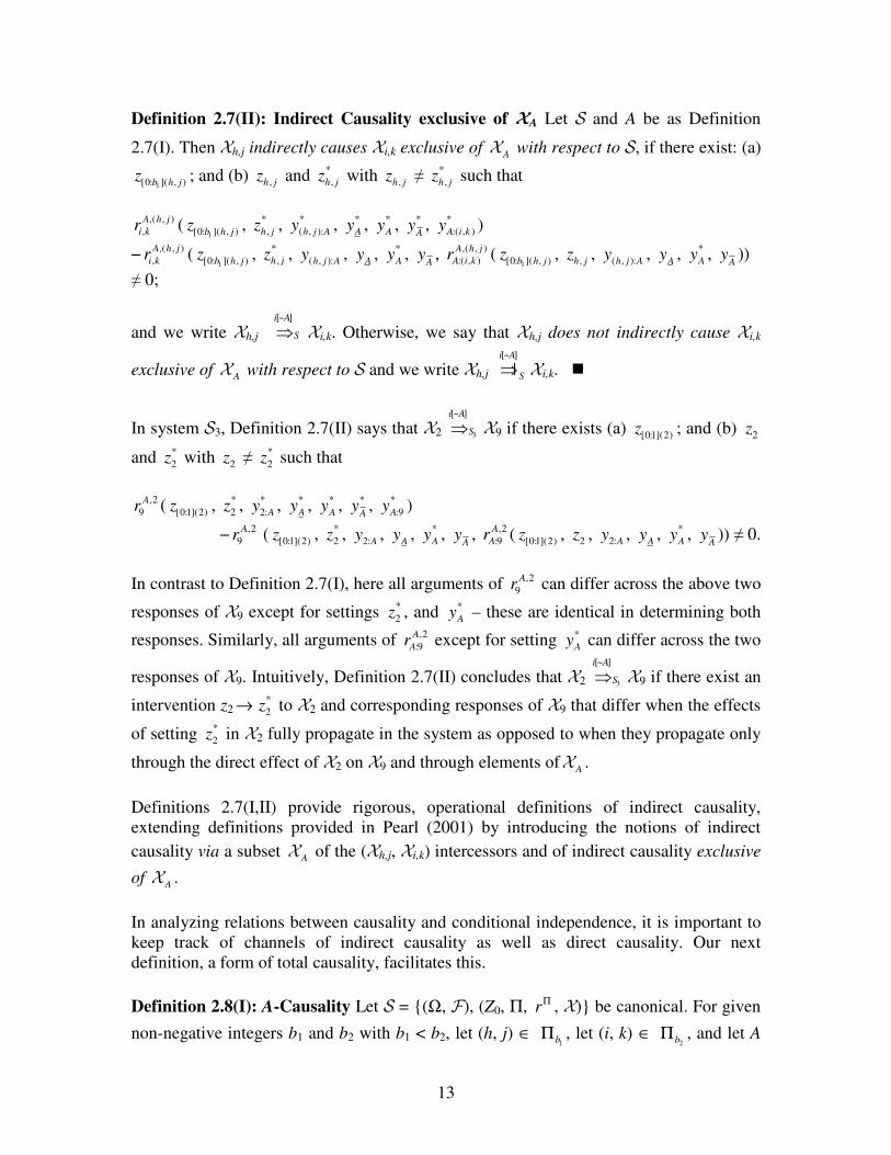
Definition 2.7(II): Indirect Causality exclusive of XA Let S and A be as Definition

2.7(I). Then Xh,j indirectly causes Xi,k exclusive of AX with respect to S, if there exist: (a)

1[0: ]( , )b h jz ; and (b) ,h jz and *

,h jz with ,h jz ≠ *

,h jz such that

,( , )

,

A h j

i kr (1[0: ]( , )b h j

z , *

,h jz , *

( , ):h j Ay , *

Ay , *

Ay , *

Ay , *

:( , )A i ky )

− ,( , )

,

A h j

i kr (1[0: ]( , )b h j

z , *

,h jz , ( , ):h j Ay ,

Ay , *

Ay ,

Ay , ,( , )

:( , )

A h j

A i kr (1[0: ]( , )b h j

z , ,h jz , ( , ):h j Ay ,

Ay , *

Ay ,

Ay ))

≠ 0;

and we write Xh,j [~ ]

i A

S⇒ Xi,k. Otherwise, we say that Xh,j does not indirectly cause Xi,k

exclusive of AX with respect to S and we write Xh,j

[~ ]

|i A

S⇒ Xi,k.

In system S3, Definition 2.7(II) says that X2 3

[~ ]

i A

S⇒ X9 if there exists (a) [0:1](2)z ; and (b) 2z

and *

2z with 2z ≠ *

2z such that

,2

9

Ar ( [0:1](2)z , *

2z , *

2:Ay , *

Ay , *

Ay , *

Ay , *

:9Ay )

− ,2

9

Ar ( [0:1](2)z , *

2z , 2:Ay , A

y , *

Ay ,

Ay , ,2

:9

A

Ar ( [0:1](2)z , 2z , 2:Ay , A

y , *

Ay ,

Ay )) ≠ 0.

In contrast to Definition 2.7(I), here all arguments of ,2

9

Ar can differ across the above two

responses of X9 except for settings *

2z , and *

Ay – these are identical in determining both

responses. Similarly, all arguments of ,2

:9

A

Ar except for setting *

Ay can differ across the two

responses of X9. Intuitively, Definition 2.7(II) concludes that X2 3

[~ ]

i A

S⇒ X9 if there exist an

intervention z2 → *

2z to X2 and corresponding responses of X9 that differ when the effects

of setting *

2z in X2 fully propagate in the system as opposed to when they propagate only

through the direct effect of X2 on X9 and through elements ofAX .

Definitions 2.7(I,II) provide rigorous, operational definitions of indirect causality,

extending definitions provided in Pearl (2001) by introducing the notions of indirect

causality via a subset AX of the (Xh,j, Xi,k) intercessors and of indirect causality exclusive

of AX .

In analyzing relations between causality and conditional independence, it is important to

keep track of channels of indirect causality as well as direct causality. Our next

definition, a form of total causality, facilitates this.

Definition 2.8(I): A-Causality Let S = (Ω, F), (Z0, Π, rΠ , X) be canonical. For given

non-negative integers b1 and b2 with b1 < b2, let (h, j) ∈ 1bΠ , let (i, k) ∈

2bΠ , and let A

14

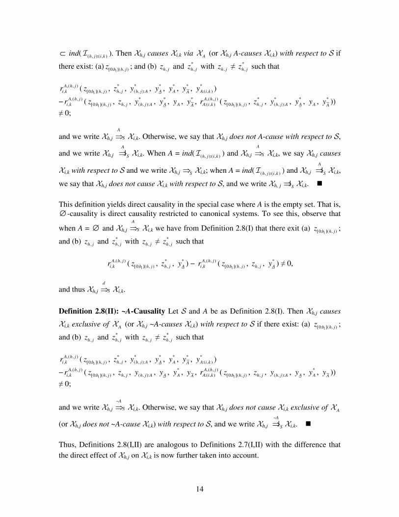
⊂ ind( ( , ):( , )h j i kI ). Then Xh,j causes Xi,k via AX (or Xh,j A-causes Xi,k) with respect to S if

there exist: (a)1[0: ]( , )b h j

z ; and (b) ,h jz and *

,h jz with ,h jz ≠ *

,h jz such that

,( , )

,

A h j

i kr (1[0: ]( , )b h j

z , *

,h jz , *

( , ):h j Ay , *

Ay , *

Ay , *

Ay , *

:( , )A i ky )

− ,( , )

,

A h j

i kr (1[0: ]( , )b h j

z , ,h jz , *

( , ):h j Ay , *

Ay , A

y , *

Ay , ,( , )

:( , )

A h j

A i kr (1[0: ]( , )b h j

z , *

,h jz , *

( , ):h j Ay , *

Ay , A

y , *

Ay ))

≠ 0;

and we write Xh,j

A

S⇒ Xi,k. Otherwise, we say that Xh,j does not A-cause with respect to S,

and we write Xh,j |A

S⇒ Xi,k. When A = ind( ( , ):( , )h j i kI ) and Xh,j

A

S⇒ Xi,k, we say Xh,j causes

Xi,k with respect to S and we write Xh,j S⇒ Xi,k; when A = ind( ( , ):( , )h j i kI ) and Xh,j |A

S⇒ Xi,k,

we say that Xh,j does not cause Xi,k with respect to S, and we write Xh, j |S⇒ Xi,k.

This definition yields direct causality in the special case where A is the empty set. That is,

∅ -causality is direct causality restricted to canonical systems. To see this, observe that

when A = ∅ and Xh,j

A

S⇒ Xi,k we have from Definition 2.8(I) that there exit (a) 1[0: ]( , )b h j

z ;

and (b) ,h jz and *

,h jz with ,h jz ≠ *

,h jz such that

,( , )

,

A h j

i kr (1[0: ]( , )b h j

z , *

,h jz , *

Ay ) − ,( , )

,

A h j

i kr (1[0: ]( , )b h j

z , ,h jz , *

Ay ) ≠ 0,

and thus Xh,j

d

S⇒ Xi,k.

Definition 2.8(II): ~A-Causality Let S and A be as Definition 2.8(I). Then Xh,j causes

Xi,k exclusive of AX (or Xh,j ~A-causes Xi,k) with respect to S if there exist: (a)

1[0: ]( , )b h jz ;

and (b) ,h jz and *

,h jz with ,h jz ≠ *

,h jz such that

,( , )

,

A h j

i kr (1[0: ]( , )b h j

z , *

,h jz , *

( , ):h j Ay , *

Ay , *

Ay , *

Ay , *

:( , )A i ky )

− ,( , )

,

A h j

i kr (1[0: ]( , )b h j

z , ,h jz , ( , ):h j Ay ,

Ay , *

Ay ,

Ay , ,( , )

:( , )

A h j

A i kr (1[0: ]( , )b h j

z , ,h jz , ( , ):h j Ay ,

Ay , *

Ay ,

Ay ))

≠ 0;

and we write Xh,j ~

A

S⇒ Xi,k. Otherwise, we say that Xh,j does not cause Xi,k exclusive of AX

(or Xh,j does not ~A-cause Xi,k) with respect to S, and we write Xh,j ~

|A

S⇒ Xi,k.

Thus, Definitions 2.8(I,II) are analogous to Definitions 2.7(I,II) with the difference that

the direct effect of Xh,j on Xi,k is now further taken into account.

15

Observe that ~ ∅ -Causality is equivalent to A-Causality with A = ind( ( , ):( , )h j i kI ). To see

this, let A = ind( ( , ):( , )h j i kI ) and suppose that Xh,j

A

S⇒ Xi,k; then Xh,j S⇒ Xi,k. We have from

Definition 2.8(I) that there exist: (a)1[0: ]( , )b h j

z ; and (b) ,h jz and *

,h jz with ,h jz ≠ *

,h jz such

that

,( , )

,

A h j

i kr (1[0: ]( , )b h j

z , *

,h jz , *

Ay ) − ,( , )

,

A h j

i kr (1[0: ]( , )b h j

z , ,h jz , A

y ) ≠ 0.

Also, let B = ∅ and suppose that Xh,j ~

B

S⇒ Xi,k. We have from Definition 2.8(II) that there

exist: (a) 1[0: ]( , )b h j

z ; and (b) ,h jz and *

,h jz with ,h jz ≠ *

,h jz such that

,( , )

,

B h j

i kr (1[0: ]( , )b h j

z , *

,h jz , *

By ) − ,( , )

,

B h j

i kr (1[0: ]( , )b h j

z , ,h jz , B

y ) ≠ 0.

But when B = ∅ , we have B = ind( ( , ):( , )h j i kI ) = A. The claim is verified, as the two

definitions coincide.

It can be analogously shown that ∅ -Causality is equivalent to ~A-Causality when A =

ind( ( , ):( , )h j i kI ). Thus, ∅ -causality and ~A-Causality with A = ind( ( , ):( , )h j i kI ) both reduce to

direct causality in canonical systems.

Our first formal result links A-causality, direct causality, and indirect causality via XA.

Proposition 2.9: Let S = (Ω, F), (Z0, Π, rΠ , X) be canonical. For given non-negative

integers b1 and b2 with b1 < b2, let (h, j) ∈ 1bΠ , let (i, k) ∈

2bΠ , let A ⊂ ind( ( , ):( , )h j i kI ),

and suppose that Xh,j

A

S⇒ Xi,k. Then Xh,j

d

S⇒ Xi,k or Xh,j [ ]

i A

S⇒ Xi,k or both.

An important special case of Proposition 2.9 occurs when A = ind( ( , ):( , )h j i kI ).

Corollary 2.10: Let S, (h, j), and (i, k) be as in Proposition 2.9, and suppose that Xh,j S⇒

Xi,k. Then Xh,j

d

S⇒ Xi,k or Xh,j

i

S⇒ Xi,k or both.

Corollary 2.10 verifies the plausible claim that if Xh,j causes Xi,k, it does so directly,

indirectly, or both. The converse need not hold, however, as direct and indirect causal

channels can cancel one another. Proposition 2.9 extends this proposition to A-causality.

A similar result holds for ~A-causality:

16

Proposition 2.11: Let S, (h, j), (i, k), and A be as in Proposition 2.9, and suppose that Xh,j

~

A

S⇒ Xi,k. Then Xh,j

d

S⇒ Xi,k or Xh,j [~ ]

i A

S⇒ Xi,k or both.

3. Independence in Settable Systems

Our next result plays a key role in formalizing Reichenbach’s principle of common cause.

Lemma 3.1: Let S = (Ω, F), (Z0, Π, rΠ , X) be canonical. Then a settable variable Xh,j

is constant if and only if X0 |S⇒ Xh,j.

So far, none of our definitions or results have required any probabilistic elements. Our

next result, formalizing Reichenbach’s principle of common cause, relates the

functionally defined notion of causality adopted here to the stochastic concept of

dependence. This requires us to explicitly introduce probability measures P on (Ω, F).

For canonical systems S, the stochastic behavior of settings and responses is determined

entirely by P and rΠ . In stating our results, we follow Dawid (1979) and write X ⊥ Y

when random variables X and Y are independent under P, whereas X ⊥/ Y means that X

and Y are not independent under P.

Proposition 3.2: The Reichenbach Principle of Common Cause (I) Let S = (Ω, F),

(Z0, Π, rΠ , X) be canonical. For given non-negative integers b1 and b2, let (h, j) ∈ 1bΠ

and (i, k) ∈ 2bΠ ((h, j) ≠ (i, k)). Let Xh,j and Xi,k be settable variables, and let Yh,j ≡

Xh,j(0, .

), and Yi,k ≡ Xi,k (0, . ). For every probability measure P on (Ω, F), if Yh,j ⊥/ Yi,k,

then either:

(i) Xh,j |S⇒ Xi,k, Xi,k |S⇒ Xh,j, and X0 S⇒ Xh,j and X0 S⇒ Xi,k; or

(ii) Xi,k |S⇒ Xh,j and either (a) (h, j) = 0 and Xh,j S⇒ Xi,k or (b) (h, j) ≠ 0 and X0 S⇒ Xh,j

and X0 S⇒ Xi,k ; or

(iii) Xh,j |S⇒ Xi,k and either (a) (i, k) = 0 and Xi,k S⇒ Xh,j or (b) (i, k) ≠ 0 and X0 S⇒ Xi,k

and X0 S⇒ Xh,j .

This result provides a fully explicit statement of conditions, both causal and stochastic,

under which the Reichenbach principle of common cause holds -- that is, under which it

is true that when two random variables in a causal system are stochastically dependent,

either one causes the other or there exists an underlying common cause. Note that the

possibility that one variable causes the other is not explicit in (ii), except when (h, j) = 0.

The possibility that Xh,j S⇒ Xi,k when (h, j) ≠ 0 is nevertheless implicit, as one way in

17

which we may have X0 S⇒ Xi,k is via the indirect channel X0 S⇒ Xh,j S⇒ Xi,k. If this fails

in (ii), then there nevertheless must be a common cause, X0. (The analogous statement

also holds in (iii).)

Although Reichenbach’s principle holds generally for canonical systems, the proof

reveals that this is not a particularly deep fact. The reason is that the fundamental settable

variable X0 can always serve as a common cause. Moreover, because the fundamental

settings Z0 can, without loss of generality, be identified with the underlying elements ω of

the universe Ω, one cannot dispense with this universal common cause without

dispensing with the underlying structure supporting probability statements.

Another way of appreciating the content of the common cause principle is to examine

what it tells us about lack of dependence, via the contrapositive of Proposition 3.2.

Specifically, the contrapositive says that, for all probability measures, if two random

variables neither cause each other nor share the common cause X0, then they are

independent. But Lemma 3.1 implies that when two random variables do not share the

common cause X0, then at least one of them must be constant. Knowing that if at least

one of two random variables is constant, then the two are independent for all probability

measures does not afford deep insight into independence. Nevertheless, deeper insights

emerge when we relax Reichenbach’s principle to its conditional counterpart in Section 4

and study its relationship to notions of d /D-separation in Section 5.

The principle of common cause gives necessary but not sufficient causal conditions for

dependence. Thus, its contrapositive gives sufficient but not necessary conditions for

independence. Specifically, independence between responses can arise in the presence of

a common cause other than the universal common cause. Independence can also arise

between two responses in the presence of an underlying causal relation.

Examples in which two independent non-constant responses share one or more common

causes are ubiquitous. Examples involving just one common cause typically require

seemingly strange or artificial (but nevertheless well defined and measurable) response

functions. On the other hand, examples of independent responses determined by two or

more common causes can arise from familiar and well-behaved functions. For example,

Cochran’s theorem (Cochran, 1934), which underlies the behavior of the standard t- and

F- statistics for hypothesis testing, ensures the independence of two distinct functions of

the squares of two or more independent identically distributed normal random variables.

It is also easy to construct examples in which independence holds between directly

causally related variables. Specifically, suppose X1 S⇒ X3 and X2 S⇒ X3 such that

Y3 c

= a Z2 + Z1,

18

where Z1 and Z2 are jointly normally distributed with mean zero and variance one.

(Following WC, we use the c

= symbol instead of the usual equality sign to emphasize that

this is a causal relationship.) Then Y3 and Z2 are also jointly normally distributed with

mean zero. Thus, if Y3 and Z2 have zero correlation, then they are independent. But this

can be ensured by taking a = − ρ, where ρ is the correlation between Z1 and Z2. (Note that

Y3 has non-zero variance as long as | a | < 1.)

It is thus useful to refine the possibilities for independence to distinguish situations in

which causal restrictions among settable variables ensure that their responses are

independent for any probability measure and those where independence among random

variables is due to a particular choice of P or a particular configuration of the response

functions. The following definitions are useful for this.

Definition 3.3: Causal Isolation and Stochastic Isolation Let S, Xh,j, Xi,k be as in

Proposition 3.2. Suppose that (a) (h, j) = 0 and Xh,j |S⇒ Xi,k; or (b) (i, k) = 0 and Xi,k |S⇒

Xh,j; or (c) (h, j) ≠ 0, (i, k) ≠ 0, and X0 |S⇒ Xh,j or X0 |S⇒ Xi,k. Then Xh,j and Xi,k are

causally isolated. Put Yh,j ≡ Xh,j (0, .) and Yi,k ≡ Xi,k (0,

. ). If P is a probability measure

on (Ω, F) such that Yh,j ⊥ Yi,k when Xh,j and Xi,k are not causally isolated, then we say

that P stochastically isolates Xh,j and Xi,k.

Thus, Xh,j and Xi,k are causally isolated when the conclusion of Proposition 3.2 does not

hold, that is, when X0 |S⇒ Xh,j or X0 |S⇒ Xi,k. Causal isolation arises when, for one or the

other of Xh,j and Xi,k, the effects of the fundamental cause X0 operate through multiple

indirect channels in just the right way as to cancel out. For variables that are not causally

isolated, independence (stochastic isolation) can arise either directly from P (e.g., when

Xh,j and Xi,k are both caused solely and directly by X0) or from just the right interaction

between multiple causes (common or direct) and the probability measure P, as in the

example preceding Definition 3.3.

Stochastic isolation is a very strong restriction on P. Nevertheless, there always exists a

stochastically isolating probability measure. In fact, we can always construct a

probability measure P on (Ω, F) that is capable of ensuring the stochastic independence

of any two random variables in S regardless of the causal relations that hold among them.

Proposition 3.4 formalizes this.

Proposition 3.4: Let S = (Ω, F), (Z0, Π, rΠ , X) be canonical. Let P be a probability

measure on (Ω, F) such that Yh,j ≡ Xh,j (0, . ) and Yi,k ≡ Xi,k (0,

. ) have probability

distributions Ph,j and Pi,k, respectively. Then there exists a probability measure *P on (Ω,

F) such that *

,h jP = Ph,j, *

,i kP = Pi,k, and the joint probability distribution of Yh,j and Yi,k is

19

*

,h jP*

,i kP . In particular, if Xh,j and Xi,k are not causally isolated, then *P stochastically

isolates Xh,j and Xi,k.

It follows from Proposition 3.4 that the converse of Proposition 3.2 does not hold. That

is, for any canonical system S, we can always find a probability measure *P such that

Xh,j and Xi,k are not causally isolated and Yh,j ⊥ Yi,k.

We are now ready to state necessary and sufficient conditions for probabilistic

dependence among random variables in settable systems.

Corollary 3.5: The Reichenbach Principle of Common Cause (II) Suppose the

conditions of Proposition 3.2 hold. For every probability measure P on (Ω, F), Yh,j ⊥/ Yi,k

if and only if (a) either:

(i) (h, j) = 0 and Xh,j S⇒ Xi,k; or

(ii) (i, k) = 0 and Xi,k S⇒ Xh,j; or

(iii) (h, j) ≠ 0, (i, k) ≠ 0, and X0 S⇒ Xi,k and X0 S⇒ Xh,j ;

and (b) P does not stochastically isolate Xh,j and Xi,k.

Stated in the contrapositive, the key idea is deceptively straightforward: Yh,j and Yi,k are

independent if and only if (a) Xh,j and Xi,k are causally isolated or (b) they are not causally

isolated (so that Yh,j and Yi,k are nondegenerate) and P stochastically isolates Xh,j and Xi,k.

This result serves several purposes. First, it characterizes stochastic dependence (and thus

independence) in terms of functionally defined causal relations, rigorously establishing

and refining the Reichenbach principle. Second, it demonstrates the crucial and

dramatically simplifying role played by the fundamental variable X0 as a universal

common cause. Once this role is accepted and understood in the context of canonical

settable systems, the content of the Reichenbach principle is no longer mysterious, nor is

it apparently deep. Third, and of particular significance, this result provides an accessible

template for understanding the more involved relations between causal structure and

conditional independence. In turn, these relations are central to the identification of

causal effects in observational studies. We thus now direct our attention to the relations

between causality and conditional independence.

4. Conditional Independence in Settable Systems

First, we state a result analogous to Lemma 3.1 that plays a key role in formalizing our

conditional Reichenbach principle of common cause.

20

Lemma 4.1 Let S, (h, j), (i, k), and A ⊂ ind( ( , ):( , )h j i kI ) be as in Definition 2.8 (I, II). Then

there exists a measurable function ,( , )

,

A h j

i kr such that

,( , )

,

A h j

i kr (1[0: ]( , )b h j

z , A

y ) = ,( , )

,

A h j

i kr (1[0: ]( , )b h j

z , ,h jz , ( , ):h j Ay ,

Ay ,

Ay ,

Ay , :( , )A i k

y )

if and only if Xh,j ~

|A

S⇒ Xi,k.

In particular, there exists a measurable function ,0

,

A

i kr such that

,0

,

A

i kr (A

y ) = ,0

,

A

i kr ( 0z , 0:Ay , A

y , A

y , A

y , :( , )A i ky )

if and only if X0 ~

|A

S⇒ Xi,k.

When A = ∅ , Lemma 4.1 contains the result of Lemma 3.1 as a special case. In fact,

when A = ∅ we have from Lemma 4.1 that there exists a measurable function ,0

,

A

i kr such

that

,0

,

A

i kr (A

y ) = ,0

,

A

i kr ( 0z , A

y )

if and only if X0 ~

|S

∅

⇒ Xi,k. It follows by canonicality that the response of Xi,k is equal to

,0

,

A

i kr (A

y ), which must be constant. Recalling that X0 ~

|S

∅

⇒ Xi,k is equivalent to X0 |S⇒ Xi,k

establishes that this is precisely the content of Lemma 3.1.

We are now ready to formalize the conditional Reichenbach principle of common cause.

Proposition 4.2: Conditional Reichenbach Principle of Common Cause (I) Let S =

(Ω, F), (Z0, Π, rΠ , X) be canonical. For given non-negative integers b1 and b2, let (h,

j) ∈ 1bΠ and (i, k) ∈

2bΠ ((h, j) ≠ (i, k)). Let Xh,j and Xi,k be settable variables, and let Yh,j

≡ Xh,j (0, .

) and Yi,k ≡ Xi,k (0, . ). Let A ⊂

1 21:[max( , ) 1]b b −∏ \ (h, j), (i, k), let XA be the

corresponding vector of settable variables, and let YA = XA (0, .

). For every probability

measure P on (Ω, F), if Yh,j ⊥/ Yi,k | YA then either:

(i) Xh,j |S⇒ Xi,k, Xi,k |S⇒ Xh,j, and with A1 ≡ A ∩ ind( 0:( , )h jI ) and A2 ≡ A ∩ ind( 0:( , )i kI ),

X0 1~

A

S⇒ Xh,j and X0 2~

A

S⇒ Xi,k; or

21

(ii) Xi,k |S⇒ Xh,j and either (a) (h, j) = 0 and Xh,j 2~

A

S⇒ Xi,k or (b) (h, j) ≠ 0 and X0 1~

A

S⇒ Xh,j

and X0 2~

A

S⇒ Xi,k ; or

(iii) Xh,j |S⇒ Xi,k and either (a) (i, k) = 0 and Xi,k 1~

A

S⇒ Xh,j or (b) (i, k) ≠ 0 and X0 2~

A

S⇒ Xi,k

and X0 1~

A

S⇒ Xh,j.

Proposition 4.2 is an explicit statement of causal and stochastic conditions that extend

Reichenbach’s principle to its conditional counterpart. This is significant, as it implies

that in recursive causal systems, knowledge of conditional dependence relations such as

Yh,j ⊥/ Yi,k | YA is informative about the possible causal relations that involve settable

variables Xh,j and Xi,k. Proposition 4.2 implies that in recursive systems, in order for two

random variables Yh,j and Yi,k to be conditionally dependent given a vector of random

variables YA, it must be that the fundamental variable X0 causes at least Xh,j or Xi,k

exclusive of the relevant subsets of XA. Otherwise, we can express Yh,j or Yi,k (or both) as

a function of the relevant sub-vector of YA. As Proposition 4.2 has A ⊂ 1 21:[max( , ) 1]b b −∏ , it is

necessary that 0 ∉ A. In fact, let Xh,j and Xi,k be as in Proposition 4.2, let B ⊂

1 20:[max( , ) 1]b b −∏ with 0 ∈ B, let XB be the corresponding vector of settable variables, and let

YB = XB (0, .

). Then it is straightforward to show that for every probability measure P on

(Ω, F), Yh,j ⊥ Yi,k | YB.

The contrapositive of Proposition 4.2 gives conditions sufficient for Yh,j ⊥ Yi,k | YA. In

Section 5, we describe how the notions of d-separation and D-separation provide

sufficient conditions for conditional independence, and we discuss how our present

results relate to these. For now, we illustrate by applying Proposition 4.2 to system S3.

We have Y0 ⊥ Yn | Y2 for n = 3, …, 8, as X0 ~2

|S⇒ Xn for n = 3, …, 8. Similarly, Y0 ⊥ Y9 |

(Y1, Y2), as X0 ~1,2

| S⇒ X9. Also, we have that Y2 ⊥ Y5 | Y3, since X0 ~3

|S⇒ X5. Similarly, we

have Y2 ⊥ Y7 | (Y3, Y6), as X0 ~3,6

| S⇒ X7. In addition, we have that Y3 ⊥ Y5 | Y2, as X0 ~2

|S⇒

X3 and X0 ~2

|S⇒ X5. Observe, however, that in G3 we have that X3 and X5 are not d-

separated given X2, although they are D-separated given X2. Similar arguments establish

that Y3 ⊥ Y4 | Y2, even though in G3 we have that X3 and X4 are not d-separated given X2.

None of the cases we have just considered require knowledge of the response functions.

This knowledge may, however, be important. To illustrate, consider determining whether

Y2 ⊥ Y7 | Y3. From the contrapositive of Proposition 4.2 we know that this will hold if X0

22

~3

|S⇒ X7. However, determining whether X0 ~3

|S⇒ X7 unavoidably requires knowledge of the

functional forms of the response functions involved. Because the path X2, X6, X7 does

not contain X3, we have that X2 and X7 are neither d-separated nor D-separated given X3

in G3. To conclude that Y2 ⊥/ Y7 | Y3 in such situations, Pearl (2000, p. 48-49) and Spirtes

et al (1993, p. 35, 56) introduce the assumptions of “stability” or “faithfulness” of P.

Proposition 4.2 does not impose such restrictions on P; instead the properties of the

response functions play the key role.

Parallel to Definition 3.3, we now provide definitions useful in distinguishing between

situations in which causal restrictions among settable variables ensure that their responses

are conditionally independent for any probability measure and those where conditional

independence among random variables is due to a particular choice of P or a particular

configuration of the response functions.

Definition 4.3: Conditional Causal Isolation and Conditional Stochastic Isolation Let

S, Xh,j, Xi,k, XA, A1, and A2 be as in Proposition 4.2. Suppose that (a) (h, j) = 0 and Xh,j

2~

|A

S⇒ Xi,k; or (b) (i, k) = 0 and Xi,k 1~

|A

S⇒ Xh,j; or (c) (h, j) ≠ 0, (i, k) ≠ 0, and X0 1~

|A

S⇒ Xh,j or X0

2~

|A

S⇒ Xi,k, then Xh,j and Xi,k are causally isolated given XA (or XA-conditionally causally

isolated). Put Yh,j ≡ Xh,j(0, . ), Yi,k ≡ Xi,k (0,

. ), and YA ≡ XA (0,

. ). If P is a probability

measure on (Ω, F) such that Yh,j ⊥ Yi,k | YA when Xh,j and Xi,k are not causally isolated

given XA, then we say that P stochastically isolates Xh,j and Xi,k given XA (or P

stochastically XA-conditionally isolates Xh,j and Xi,k).

From Definition 4.3, we have that Xh,j and Xi,k are causally isolated given XA when the

conclusion of Proposition 4.2 does not hold, that is when X0 1~

|A

S⇒ Xh,j or X0 2~

|A

S⇒ Xi,k. Just

as in the unconditional case, stochastic isolation given XA is a nontrivial restriction on P.

However, for sufficiently well behaved probability measures, there always exists such a

stochastically isolating P. In particular, if given YA, the conditional probabilities of Yh,j

and Yi,k are regular (see e.g. Dudley, 2002, p. 268-270), then one can always construct a

probability measure ensuring that Yh,j and Yi,k are conditionally independent given YA. The

next result formally establishes this.

Proposition 4.4: Let S = (Ω, F), (Z0, Π, rΠ , X) be canonical. Let P be a probability

measure on (Ω, F) such that given YA ≡ XA (0, . ), the responses Yh,j ≡ Xh,j(0,

.) and Yi,k ≡

Xi,k (0, . ) have regular conditional probability distributions , |h j AP and , |i k AP , respectively.

Then there exists a probability measure *P on (Ω, F) such that given YA, the conditional

probability distributions of Yh,j and Yi,k, *

, |h j AP and *

, |i k AP , respectively, satisfy *

, |h j AP = , |h j AP ,

23

*

, |i k AP = , |i k AP , and the conditional joint probability distribution of Yh,j and Yi,k is *

, |h j AP*

, |i k AP .

In particular, if Xh,j and Xi,k are not causally isolated given XA, then *P stochastically

isolates Xh,j and Xi,k given XA.

Analogous to Corollary 3.6, our next result provides necessary and sufficient conditions

for conditional dependence among random variables Yh,j and Yi,k in canonical systems

given a vector of random variables YA corresponding to a subset XA of the (Xh,j , Xi,k)

intercessors.

Corollary 4.5: Conditional Reichenbach Principle of Common Cause (II) Suppose

the conditions of Proposition 4.2 hold. For every probability measure P on (Ω, F), Yh,j ⊥/

Yi,k | YA if and only if (a) either

(i) (h, j) = 0 and with A2 ≡ A ∩ ind( ( )

0:( , )

d

i k

SI ), Xh,j

2~

A

S⇒ Xi,k; or

(ii) (i, k) = 0 and with A1 ≡ A ∩ ind( ( )

0:( , )

d

h j

SI ),Xi,k

1~

A

S⇒ Xh,j; or

(iii) (h, j) ≠ 0, (i, k) ≠ 0, and X0 2~

A

S⇒ Xi,k and X0 1~

A

S⇒ Xh,j;

and (b) P does not stochastically isolate Xh,j and Xi,k given XA.

Corollary 4.5 tells us that, for all probability measures, if two settable variables neither

cause each other exclusive of the relevant elements of XA nor have a common cause

exclusive of the relevant elements of XA, then their responses are conditionally

independent given YA. In fact, Lemma 4.1 implies that when two non-degenerate random

variables do not share a common cause exclusive of the relevant subsets of XA, then at

least one of them must be a function only of the relevant subs-vector of YA. In addition,

Corollary 4.5 tells us that conditional independence can also occur when Xh,j and Xi,k are

not causally isolated given XA, provided P stochastically isolates Xh,j and Xi,k given XA.

For example, in system S3 suppose that P stochastically isolates X1 and X4 given X3; then

we have that Y1 ⊥ Y4 | Y3 even though X1 and X4 are neither d-separated nor D-separated

given X3 in G3.

In applications, we are usually interested in conditional independence relations between

vectors of variables. Accordingly, we now generalize the results of this section to

accommodate vectors of variables.

First, we note that the meaning of the notations

d

S⇒ and |d

S⇒ extends to accommodate

disjoint sets of multiple settable variables appearing on the right and left hand sides. For

24

example, if A and B are non-empty collections of indexes, we let XA be a vector of

settable variables whose indexes belong to A and similarly for XB, and we write XA

d

S⇒

XB if Xh,j

d

S⇒ Xi,k for some (h, j) ∈ A and (i, k) ∈ B. Otherwise, we write XA |d

S⇒ XB

indicating that Xh,j |d

S⇒ Xi,k for all (h, j) ∈ A and (i, k) ∈ B. Observe that even though S is

a recursive system, it is possible to have XA

d

S⇒ XB and XB

d

S⇒ XA.

Similarly, we can extend the meaning of the notations [ ]

i A

S⇒ , [ ]

|i A

S⇒ , [~ ]

i A

S⇒ , [~ ]

|i A

S⇒ ,

A

S⇒ , |A

S⇒ , ~

A

S⇒ ,

and ~

|A

S⇒ to accommodate disjoint sets of multiple settable variables appearing on the right

and left hand sides. To do this requires some further notation. Let :A BI = ( , )h j A∈∪ ( , )i k B∈∪

( , ):( , )h j i kI \ (XA ∪ XB) denote the set of (XA, XB) d(S)-intercessors and let C ⊂ ind( :A BI ).

For given (h, j) ∈ A and (i, k) ∈ B, let ( , ):( , )h j i kC = C ∩ ind( ( , ):( , )h j i kI ). Then, we say that

XA

C

S⇒ XB if there exists (h, j) ∈ A ∩ 1bΠ and (i, k) ∈ B ∩

2bΠ with b1 < b2, such that

Xh,j ( , ):( , )

h j i kC

S⇒ Xi,k. Otherwise, we write XA |C

S⇒ XB, indicating that Xh,j ( , ):( , )

|h j i kC

S⇒ Xi,k for all (h, j)

∈ A ∩ 1bΠ and (i, k) ∈ B ∩

2bΠ with b1 < b2. The notations other than

A

S⇒ and |A

S⇒ in

the list above are defined analogously for vectors of variables.

The definitions of conditional causal isolation and conditional stochastic isolation directly

generalize to the vector case in the obvious way. Thus, if YA ⊥ YB | YC when XA and XB

are not causally isolated given XC (that is conditions (i), (ii), or (iii) of (a) in Theorem 4.6

below hold) then we say that P stochastically isolates XA and XB given XC.

We introduce one last notation. Let a = minb: there exists (h, j) ∈ bΠ ∩ A and b =

minb: there exists (i, k) ∈ bΠ ∩ B. Similarly, Let a = maxb: there exists (h, j) ∈

bΠ ∩ A and b = maxb: there exists (i, k) ∈ bΠ ∩ B.

Theorem 4.6: Conditional Reichenbach Principle of Common Cause (III) Let S

≡ (Ω, F), (Z, Π, rΠ , X) be canonical. Let A and B be non-empty disjoint subsets of

Π ∪ Π0 , let XA and XB be the corresponding vectors of settable variables, and let YA =

XA (0, .

) and YB = XB (0, .

). Let C ⊂ 1:[max( , ) 1]a b −

∏ \ (A ∪ B), let XC be the corresponding

vector of settable variables, and let YC = XC (0, .

). For every probability measure P on (Ω,

F), YA ⊥/ YB | YC if and only if (a) either:

25

(i) a = 0, b ≠ 0, and with C2 ≡ C ∩ ind( 0:BI ), X0 2~

C

S⇒ XB; or

(ii) a ≠ 0, b = 0, and with C1 ≡ C ∩ ind( 0:AI ), X0 1~

C

S⇒ XA; or

(iii) a ≠ 0, b ≠ 0, and with C1 ≡ C ∩ ind( 0:AI ) and C2 ≡ C ∩ ind( 0:BI ), X0 1~

C

S⇒ XA

and X0 2~

C

S⇒ XB;

and (b) P does not stochastically isolate XA and XB given XC.

Corollary 4.5 obtains as a special case of Theorem 4.6 by taking A = (h, j) and B = (i,

k). Corollary 3.5 follows from Theorem 4.6 by further taking C = ∅ .

5. Settable Systems and Graphical Separation

The results of the previous section pertain directly to the artificial intelligence literature

that aims at encoding conditional independence relationships by graphical means. In

particular, as we now discuss, Proposition 4.2 and Corollary 4.5 and Theorem 4.6 relate

directly to notions of d-separation (Verma and Pearl, 1988; Geiger and Pearl, 1993; Pearl,

2000, p. 16-17), D-separation (Geiger, Verma, and Pearl, 1990), and of “separation” in

“moral graphs” (Lauritzen and Spiegelhalter, 1988; Lauritzen, Dawid, Larsen, and

Leimer, 1990).

5.1 Graphical Separation

For finite systems, Geiger, et. al. (1990) provide a set of graphical criteria for DAGs that

they refer to as d-separation that can identify exactly the conditional independence

relations that can be derived from a “recursive basis2” under a set of axioms they refer to

as the “graphoid axioms3.” Lauritzen, et. al. (1990, proposition 3) provide an equivalent

graphical algorithm applicable to the “moral” graph of the smallest relevant “ancestral”

sets in the original DAG.

2 To express the Geiger, et. al. (1990) notion of a recursive basis in our framework, let H and Jh be finite

integers, and let ( , )h jP , h = 1, …, H; j = 1, …, Jh, be the set of Xh,j d(S)-predecessors. A recursive basis is

then a list of conditional independence statements, one for every (h, j), of the form Yh,j ⊥ ( )( , )( , ) \

dh jh j B

Y SP

|

,h jBY for some

( , )h jB ⊂

( , )h jP .

3 In Geiger, et. al. (1990), the four graphoid axioms are properties of conditional independence relations

discussed, for example, in Dawid (1979). Geiger, et. al. (1990) list, but do not use, a fifth axiom they refer

to as the “intersection” axiom, which does not hold for all probability measures. A sufficient but not

necessary condition under which the intersection axiom holds is that the probability measure P is strictly

positive in the sense that for any event A in F, we have P(A) = 0 only if A = ∅ (Verma and Pearl 1988;

Geiger and Pearl 1993; Pearl 2000). San Martin, Mouchart, and Rolin (2005, theorem 2.2) employ the

concept of “no common information” or “measurable separability” to provide a weaker condition under

which the intersection axiom holds.

26

A key assumption in the d-separation literature is that the governing probability measure

P obeys a “directed local Markov property” (Lauritzen, et. al., 1990). This is the

assumption that conditioning on the direct causes of a variable (its “parents”) renders it

conditionally independent from its remaining predecessors. Pearl (2000, theorem 1.2.7)

calls this the “parental Markov condition” and Spirtes, Glymour, and Scheines (1993, p.

54) refer to it as the “Causal Markov Property.”

Lauritzen, et. al. (1990) further show that this property is equivalent to two other

properties that they refer to as the “directed global Markov property” and the “well-

numbering Markov property” (Lauritzen, et. al. 1990, corollary 2). When P is absolutely

continuous with respect to a product measure, the directed local Markov property is also

equivalent to P admitting a particular recursive factorization (Lauritzen, et. al., 1990,

theorem 1). Under these equivalent Markov assumptions, their graphical algorithm or

equivalently d-separation permits verification of valid conditional independence relations

from the graph (Lauritzen, et. al., 1990, proposition 2).

The literature on causality and conditional independence (e.g., Spohn, 1980; Lauritzen

and Spiegelhalter, 1988), particularly as expressed in terms of the d-separation criteria

(e.g., Pearl, 2000, p. 16-17), embodies three particular relations between causality and

conditional independence. Absent other causal relationships and expressed in the present

notation and nomenclature, these can be stated as:

d.1 Conditioning on variables that fully mediate the effect of Xh,j on Xi,k renders Yh,j and

Yi,k conditionally independent;

d.2 Conditioning on common causes of Xh,j and Xi,k, or conditioning on variables that

fully mediate the effects of these common causes on either (or both) Xh,j or Xi,k, renders

Yh,j and Yi,k conditionally independent;

d.3 Conditioning on the response of a settable variable caused by both Xh,j and Xi,k (a

“common response”) renders Yh,j and Yi,k as well as other respective successors of Xh,j and

Xi,k conditionally dependent.

D-separation adds to these the following property:

D.4 Conditioning on causes that entirely determine Xh,j renders Yh,j conditionally

independent of all other variables in the system.

D-separation accommodates the presence of “deterministic nodes” or variables that are

functionally dependent on their predecessors. Because the fundamental variable is not

represented in deterministic DAGs, random behavior is at best not explicitly treated. In

the absence of random behavior, a formal role for probability and conditional probability

is lacking. To avoid this difficulty, Pearl (2000, p. 68) analyzes “chance-node” DAGs, in

27

which every node is a function of its parents and a non-degenerate unobserved random

variable. These “arbitrary distributed random disturbances” are assumed to be “jointly

independent” and are not explicitly represented in the DAG (see Pearl, 2000, pp. 68 - 69).

Pearl (2000, p. 68) states that, “these disturbances represent independent background

factors that the investigator chooses not to include in the analysis.” In our terminology,

this amounts to assuming that the probability measure P jointly stochastically isolates

these random disturbances. This is indeed a strong assumption. Further, it is one that does

not emerge naturally from the system of interest; rather, it seems artificially annexed.

Geiger, et. al. (1990, p. 526) state explicitly that “no functional dependencies exist in this

[chance-node] interpretation of DAGs.” It follows that d-separation and D-separation

coincide in chance-node DAGs, since none of the graph’s nodes are fully determined by

its parents. This also creates a serious conceptual obstacle: applying a definition of

causality based on functional dependence to chance-node DAGs is inherently

contradictory (see Pearl, 2000, pp. 26, 68). Although Lauritzen, et. al. (1988) refer to

“causal networks” throughout, they avoid a causal interpretation based on functional

dependence, saying that “causality has a broad interpretation as any natural ordering in

which knowledge of a parent influences opinion concerning a child – this influence could

be logical, physical, temporal, or simply conceptual in that it may be most appropriate to

think of the probability of children given parents” (Lauritzen, et. al., 1988, p. 160).

Indeed, there is no reference whatsoever to causality in Lauritzen, et. al. (1990); the

discussion there is solely concerned with properties of conditional dependence and its

graphical representation. Significantly, Dawid (2002, p. 165) states that, “if we were to

base causal understanding on the structure of graphical representations, these must be

supplied with a richer semantics, already embodying causal properties.” Thus, chance-

node DAGs do not support an analysis of causality based on functional dependence of the

sort considered here. Nor does there appear to be a solid basis for using the notions of d-

separation (or D-separation) to obtain insight into the relations between conditional

probability and causal concepts based on functional relationships.

How, then, is one to interpret the statements of properties d.1 – d.3 and D.4 above, where

concepts of causality and conditional probability are explicitly intermixed? The answer is

that these statements are fully meaningful within the context of canonical settable

systems. The compatibility of the settable system framework with classical probability

theory and the above function-based definitions of direct and indirect causality enable us

to avoid the difficulties encountered by chance-node DAGs. As discussed extensively in

WC, causality is properly defined between settable variables, rather than in terms of

random variables or events. Consequently, distinctions between “deterministic” and

“chance” nodes are no longer relevant, eliminating the difficulties for causal discourse

that these distinctions create. The canonical settable system framework supplies the

“richer semantics, already embodying causal properties” for graphical representation

required by Dawid (2002).

Given that d.1– d.3 and D.4 are meaningful statements within the framework of canonical

settable systems, it is possible to investigate their validity. For this, we first note that our

results in Section 4 do not impose any “Markov” assumptions on the probability measure

28

P. Instead, the directed local Markov property is a consequence of our framework.

Specifically, the inclusion of the fundamental variable X0 and Proposition 4.2 implies that

this property always holds for canonical systems. For example, in system S3 we have that

Y3 ⊥ Y0 | Y2, Y4 ⊥ Y0 | (Y2, Y3), etc.

Further, and despite the fact that we operate only with the usual properties of conditional

probability (e.g., Dawid, 1979), Proposition 4.2 (and Corollary 4.5 and Theorem 4.6)

deliver d.1, d.2, and D.4 as necessary consequences of settable systems. That is, for

canonical systems, the conditional Reichenbach principle of common cause holds,

ensuring these three properties. Thus, not only are d.1, d.2, and D.4 fully meaningful

statements in the settable system framework, but Proposition 4.2 also demonstrates that

recursive bases, the intersection axiom, and the Markov properties are not fundamental to

establishing these interrelations between causal relations and conditional independence.

This by no means suggests that the notions of d-separation are inappropriate for the study

of conditional probability relationships; indeed they are. Rather, they are not a natural

starting point or context for a study of the interrelations between functionally defined

causality and conditional probability.

Thus, the d-separation literature provides sufficient conditions for inferring conditional

independence from graphical structures, but does not relate this to causal notions based

on functional dependence. Among other things, the d-separation conditions apply to

chance-node DAGs with a recursive basis, satisfying certain Markov properties. In

contrast, our conditional Reichenbach principle provides necessary and sufficient

conditions for inferring conditional independence from causal structures where causality

is defined in terms of functional dependence. We do not require chance nodes or

recursive bases. In addition, the Markov properties emerge as a consequence of our

structure, rather than having to be imposed. Other conditions imposed in the d-separation

framework are either consequences of our set-up or are held in common, such as the

absence of conditioning on successors.

5.2 Conditioning on Successors

Above, we have explicitly discussed d.1, d.2, and D.4, but what about property d.3? It,

too, is formally meaningful in the canonical settable system framework; but is it a

consequence of the properties of a canonical recursive settable system in the same way

that d.1, d.2, and D.4 are? We begin to address this question by noting that unlike the

latter properties, which all involve the conditional independence of successors

conditioning on predecessors, d.3 is a statement about the (lack of) conditional

independence of predecessors, conditioning on a successor. Thus, although d.3 may

indeed be a valid property of canonical systems under given conditions, it will not follow

from the conditional Reichenbach principle of common cause.

A general analysis of d.3 is sufficiently involved that a full treatment is beyond the scope

of the present treatment. First, we demonstrate in Proposition 5.1 by counterexample that

d.3 does not hold for all probability measures.

29

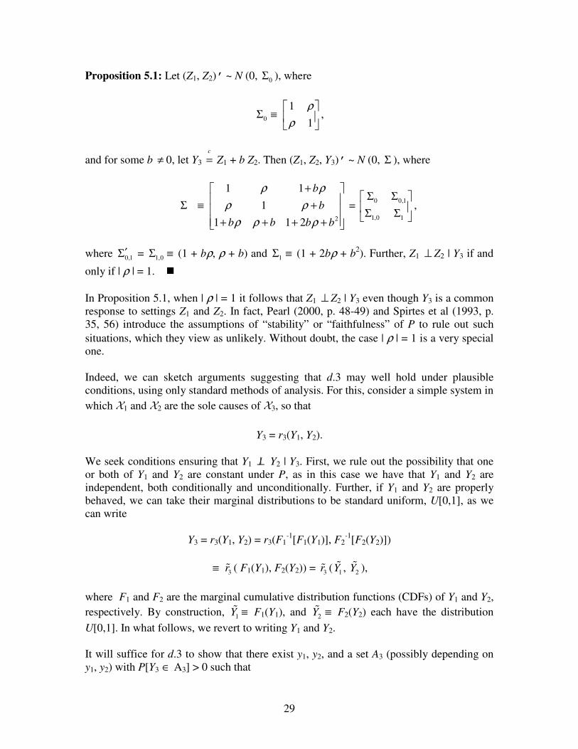
Proposition 5.1: Let (Z1, Z2)’ ~ N (0, 0Σ ), where

0Σ ≡ 1

1

ρ

ρ

,

and for some b ≠ 0, let Y3 c

= Z1 + b Z2. Then (Z1, Z2, Y3)’ ~ N (0, Σ ), where

Σ ≡ 2

1 1

1

1 1 2

b

b

b b b b

ρ ρ

ρ ρ

ρ ρ ρ

+ + + + + +

= 0 0,1

1,0 1

Σ Σ Σ Σ

,

where 0,1′Σ = 1,0Σ ≡ (1 + bρ, ρ + b) and 1Σ ≡ (1 + 2bρ + b

2). Further, Z1 ⊥ Z2 | Y3 if and

only if | ρ | = 1.

In Proposition 5.1, when | ρ | = 1 it follows that Z1 ⊥ Z2 | Y3 even though Y3 is a common

response to settings Z1 and Z2. In fact, Pearl (2000, p. 48-49) and Spirtes et al (1993, p.

35, 56) introduce the assumptions of “stability” or “faithfulness” of P to rule out such

situations, which they view as unlikely. Without doubt, the case | ρ | = 1 is a very special

one.

Indeed, we can sketch arguments suggesting that d.3 may well hold under plausible

conditions, using only standard methods of analysis. For this, consider a simple system in

which X1 and X2 are the sole causes of X3, so that

Y3 = r3(Y1, Y2).

We seek conditions ensuring that Y1 ⊥/ Y2 | Y3. First, we rule out the possibility that one

or both of Y1 and Y2 are constant under P, as in this case we have that Y1 and Y2 are

independent, both conditionally and unconditionally. Further, if Y1 and Y2 are properly

behaved, we can take their marginal distributions to be standard uniform, U[0,1], as we

can write

Y3 = r3(Y1, Y2) = r3(F1-1

[F1(Y1)], F2-1

[F2(Y2)])

≡ 3r ( F1(Y1), F2(Y2)) = 3r ( 1Y , 2Y ),

where F1 and F2 are the marginal cumulative distribution functions (CDFs) of Y1 and Y2,

respectively. By construction, 1Y ≡ F1(Y1), and 2Y ≡ F2(Y2) each have the distribution

U[0,1]. In what follows, we revert to writing Y1 and Y2.

It will suffice for d.3 to show that there exist y1, y2, and a set A3 (possibly depending on

y1, y2) with P[Y3 ∈ A3] > 0 such that

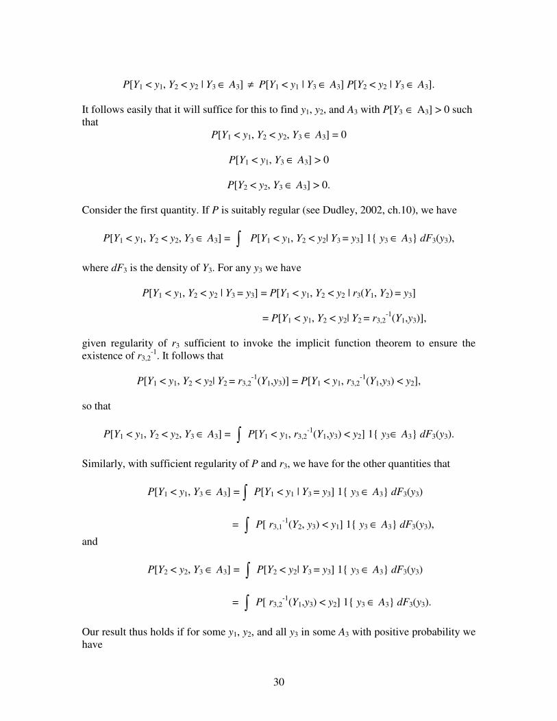
30

P[Y1 < y1, Y2 < y2 | Y3 ∈ A3] ≠ P[Y1 < y1 | Y3 ∈ A3] P[Y2 < y2 | Y3 ∈ A3].

It follows easily that it will suffice for this to find y1, y2, and A3 with P[Y3 ∈ A3] > 0 such

that

P[Y1 < y1, Y2 < y2, Y3 ∈ A3] = 0

P[Y1 < y1, Y3 ∈ A3] > 0

P[Y2 < y2, Y3 ∈ A3] > 0.

Consider the first quantity. If P is suitably regular (see Dudley, 2002, ch.10), we have

P[Y1 < y1, Y2 < y2, Y3 ∈ A3] = ∫ P[Y1 < y1, Y2 < y2| Y3 = y3] 1 y3 ∈ A3 dF3(y3),

where dF3 is the density of Y3. For any y3 we have

P[Y1 < y1, Y2 < y2 | Y3 = y3] = P[Y1 < y1, Y2 < y2 | r3(Y1, Y2) = y3]

= P[Y1 < y1, Y2 < y2| Y2 = r3,2-1

(Y1,y3)],

given regularity of r3 sufficient to invoke the implicit function theorem to ensure the

existence of r3,2-1

. It follows that

P[Y1 < y1, Y2 < y2| Y2 = r3,2-1

(Y1,y3)] = P[Y1 < y1, r3,2-1

(Y1,y3) < y2],

so that

P[Y1 < y1, Y2 < y2, Y3 ∈ A3] = ∫ P[Y1 < y1, r3,2-1

(Y1,y3) < y2] 1 y3∈ A3 dF3(y3).

Similarly, with sufficient regularity of P and r3, we have for the other quantities that

P[Y1 < y1, Y3 ∈ A3] = ∫ P[Y1 < y1 | Y3 = y3] 1 y3 ∈ A3 dF3(y3)

= ∫ P[ r3,1-1

(Y2, y3) < y1] 1 y3 ∈ A3 dF3(y3),

and

P[Y2 < y2, Y3 ∈ A3] = ∫ P[Y2 < y2| Y3 = y3] 1 y3 ∈ A3 dF3(y3)

= ∫ P[ r3,2-1

(Y1,y3) < y2] 1 y3 ∈ A3 dF3(y3).

Our result thus holds if for some y1, y2, and all y3 in some A3 with positive probability we

have

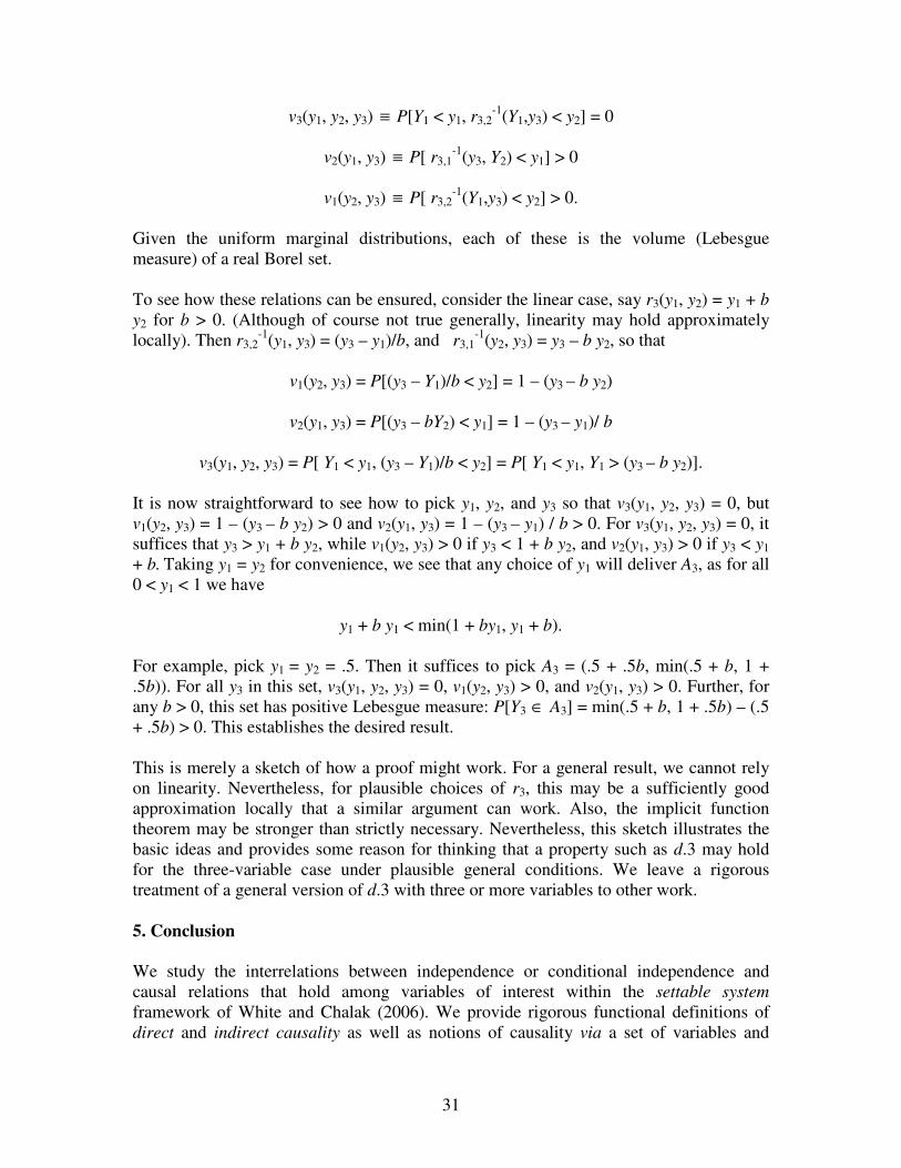
31

v3(y1, y2, y3) ≡ P[Y1 < y1, r3,2-1

(Y1,y3) < y2] = 0

v2(y1, y3) ≡ P[ r3,1-1

(y3, Y2) < y1] > 0

v1(y2, y3) ≡ P[ r3,2-1

(Y1,y3) < y2] > 0.

Given the uniform marginal distributions, each of these is the volume (Lebesgue

measure) of a real Borel set.

To see how these relations can be ensured, consider the linear case, say r3(y1, y2) = y1 + b

y2 for b > 0. (Although of course not true generally, linearity may hold approximately

locally). Then r3,2-1

(y1, y3) = (y3 – y1)/b, and r3,1-1

(y2, y3) = y3 – b y2, so that

v1(y2, y3) = P[(y3 – Y1)/b < y2] = 1 – (y3 – b y2)

v2(y1, y3) = P[(y3 – bY2) < y1] = 1 – (y3 – y1)/ b

v3(y1, y2, y3) = P[ Y1 < y1, (y3 – Y1)/b < y2] = P[ Y1 < y1, Y1 > (y3 – b y2)].

It is now straightforward to see how to pick y1, y2, and y3 so that v3(y1, y2, y3) = 0, but

v1(y2, y3) = 1 – (y3 – b y2) > 0 and v2(y1, y3) = 1 – (y3 – y1) / b > 0. For v3(y1, y2, y3) = 0, it

suffices that y3 > y1 + b y2, while v1(y2, y3) > 0 if y3 < 1 + b y2, and v2(y1, y3) > 0 if y3 < y1

+ b. Taking y1 = y2 for convenience, we see that any choice of y1 will deliver A3, as for all

0 < y1 < 1 we have

y1 + b y1 < min(1 + by1, y1 + b).

For example, pick y1 = y2 = .5. Then it suffices to pick A3 = (.5 + .5b, min(.5 + b, 1 +

.5b)). For all y3 in this set, v3(y1, y2, y3) = 0, v1(y2, y3) > 0, and v2(y1, y3) > 0. Further, for

any b > 0, this set has positive Lebesgue measure: P[Y3 ∈ A3] = min(.5 + b, 1 + .5b) – (.5

+ .5b) > 0. This establishes the desired result.

This is merely a sketch of how a proof might work. For a general result, we cannot rely

on linearity. Nevertheless, for plausible choices of r3, this may be a sufficiently good

approximation locally that a similar argument can work. Also, the implicit function

theorem may be stronger than strictly necessary. Nevertheless, this sketch illustrates the

basic ideas and provides some reason for thinking that a property such as d.3 may hold

for the three-variable case under plausible general conditions. We leave a rigorous

treatment of a general version of d.3 with three or more variables to other work.

5. Conclusion

We study the interrelations between independence or conditional independence and

causal relations that hold among variables of interest within the settable system

framework of White and Chalak (2006). We provide rigorous functional definitions of

direct and indirect causality as well as notions of causality via a set of variables and

32

exclusive of a set of variables. These definitions add to and extend the definitions

provided in SGS (1993) and Pearl (2000, 2001). We provide a proof for the Reichenbach

principle of common cause, and we introduce and prove its conditional counterpart, the

conditional Reichenbach principle of common cause. We distinguish between situations

in which causal restrictions among settable variables ensure that their responses are

(conditionally) independent for any probability measure and those where conditional

independence among random variables is due to a particular choice of the probability

measure or a particular configuration of the response functions. We introduce concepts of

(conditional) causal and stochastic isolation to support these results. We then state

necessary and sufficient conditions for (conditional) dependence among certain random

vectors in settable systems.

We relate our results to notions of d-separation, D-separation, and alternative graphical

criteria in the artificial intelligence literature. We show thereby that canonical settable

systems constitute an appropriate framework for studying the interrelations between

functionally defined causal relations and conditional independence, and that recursive

bases, the intersection axiom, and the Markov properties are not fundamental to

establishing these interrelations. In particular, we see that the “directed local Markov

property” always holds in canonical settable systems. Also, we do not impose the

assumption of “faithfulness” (SGS, 1993) or “stability” (Pearl, 2000); rather, we permit

our conclusions about causality and conditional independence to emerge from the

properties of the response functions involved. In this work, we restrict our attention to

studying the implications for conditional independence of conditioning on predecessors

of the variables of interest. We leave to other work studying the implications for

conditional independence of conditioning on successors of variables of interest, as also

considered in the d-separation literature.

We restrict attention here to recursive systems. An interesting direction for further

research is to extend our concepts and results to non-recursive systems (see, e.g.,

Lauritzen and Richardson, 2002; White, 2007). The results of the present work also have

direct implications for the structural identification of causal effects in observational

studies with use of conditioning instruments and predictive proxies discussed in WC and

Chalak and White (2006). Also, our results have direct implications for suggesting and

testing for causal models. We leave investigating these relationships to other work.

Our framework also constitutes an appropriate foundation for studying the identification

of “path-specific” causal effects (See Pearl, 2001; Avin, Shpitser, and Pearl, 2005). It

follows that this framework also provides a solid foundation for studying policy

evaluation (see, e.g., Heckman, 2005), where distinctions between direct and indirect

effects are focal. It is also of interest to investigate the relationship between our results

and notions of Granger and Sims causality (Granger, 1969; Sims, 1972). We leave these

studies to other work.

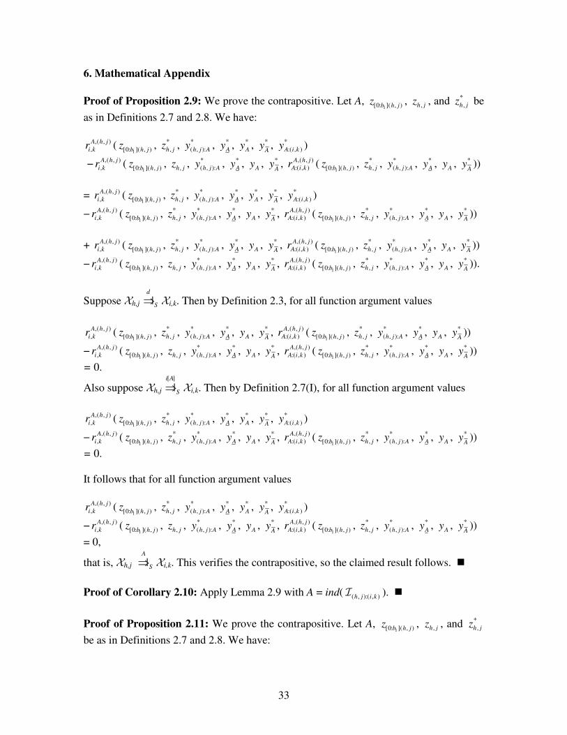
33

6. Mathematical Appendix

Proof of Proposition 2.9: We prove the contrapositive. Let A, 1[0: ]( , )b h j

z , ,h jz , and *

,h jz be

as in Definitions 2.7 and 2.8. We have:

,( , )

,

A h j

i kr (1[0: ]( , )b h j

z , *

,h jz , *

( , ):h j Ay , *

Ay , *

Ay , *

Ay , *

:( , )A i ky )

− ,( , )

,

A h j

i kr (1[0: ]( , )b h j

z , ,h jz , *

( , ):h j Ay , *

Ay , A

y , *

Ay , ,( , )

:( , )

A h j

A i kr (1[0: ]( , )b h j

z , *

,h jz , *

( , ):h j Ay , *

Ay , A

y , *

Ay ))

= ,( , )

,

A h j

i kr (1[0: ]( , )b h j

z , *

,h jz , *

( , ):h j Ay , *

Ay , *

Ay , *

Ay , *

:( , )A i ky )

− ,( , )

,

A h j

i kr (1[0: ]( , )b h j

z , *

,h jz , *

( , ):h j Ay , *

Ay , A

y , *

Ay , ,( , )

:( , )

A h j

A i kr (1[0: ]( , )b h j

z , *

,h jz , *

( , ):h j Ay , *

Ay , A

y , *

Ay ))

+ ,( , )

,

A h j

i kr (1[0: ]( , )b h j

z , *

,h jz , *

( , ):h j Ay , *

Ay , A

y , *

Ay , ,( , )

:( , )

A h j

A i kr (1[0: ]( , )b h j

z , *

,h jz , *

( , ):h j Ay , *

Ay , A

y , *

Ay ))

− ,( , )

,

A h j

i kr (1[0: ]( , )b h j

z , ,h jz , *

( , ):h j Ay , *

Ay , A

y , *

Ay , ,( , )

:( , )

A h j

A i kr (1[0: ]( , )b h j

z , *

,h jz , *

( , ):h j Ay , *

Ay , A

y , *

Ay )).

Suppose Xh,j |d

S⇒ Xi,k. Then by Definition 2.3, for all function argument values

,( , )

,

A h j

i kr (1[0: ]( , )b h j

z , *

,h jz , *

( , ):h j Ay , *

Ay , A

y , *

Ay , ,( , )

:( , )

A h j

A i kr (1[0: ]( , )b h j

z , *

,h jz , *

( , ):h j Ay , *

Ay , A

y , *

Ay ))

− ,( , )

,

A h j

i kr (1[0: ]( , )b h j

z , ,h jz , *

( , ):h j Ay , *

Ay , A

y , *

Ay , ,( , )

:( , )

A h j

A i kr (1[0: ]( , )b h j

z , *

,h jz , *

( , ):h j Ay , *

Ay , A

y , *

Ay ))

= 0.

Also suppose Xh,j [ ]

|i A

S⇒ Xi,k. Then by Definition 2.7(I), for all function argument values

,( , )

,

A h j

i kr (1[0: ]( , )b h j

z , *

,h jz , *

( , ):h j Ay , *

Ay , *

Ay , *

Ay , *

:( , )A i ky )

− ,( , )

,

A h j

i kr (1[0: ]( , )b h j

z , *

,h jz , *

( , ):h j Ay , *

Ay , A

y , *

Ay , ,( , )

:( , )

A h j

A i kr (1[0: ]( , )b h j

z , *

,h jz , *

( , ):h j Ay , *

Ay , A

y , *

Ay ))

= 0.

It follows that for all function argument values

,( , )

,

A h j

i kr (1[0: ]( , )b h j

z , *

,h jz , *

( , ):h j Ay , *

Ay , *

Ay , *

Ay , *

:( , )A i ky )

− ,( , )

,

A h j

i kr (1[0: ]( , )b h j

z , ,h jz , *

( , ):h j Ay , *

Ay , A

y , *

Ay , ,( , )

:( , )

A h j

A i kr (1[0: ]( , )b h j

z , *

,h jz , *

( , ):h j Ay , *

Ay , A

y , *

Ay ))

= 0,

that is, Xh,j |A

S⇒ Xi,k. This verifies the contrapositive, so the claimed result follows.

Proof of Corollary 2.10: Apply Lemma 2.9 with A = ind( ( , ):( , )h j i kI ).

Proof of Proposition 2.11: We prove the contrapositive. Let A, 1[0: ]( , )b h j

z , ,h jz , and *

,h jz

be as in Definitions 2.7 and 2.8. We have:

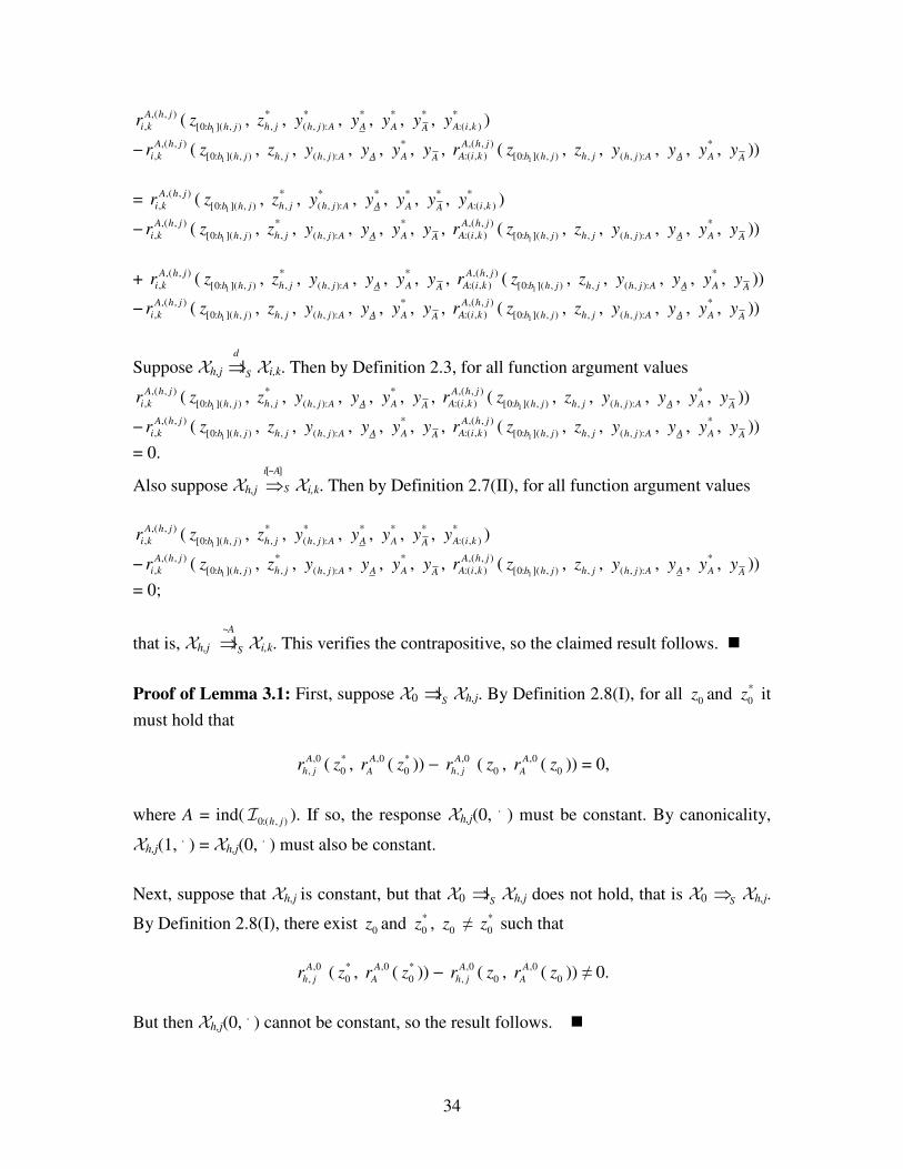
34

,( , )

,

A h j

i kr (1[0: ]( , )b h j

z , *

,h jz , *

( , ):h j Ay , *

Ay , *

Ay , *

Ay , *

:( , )A i ky )

− ,( , )

,

A h j

i kr (1[0: ]( , )b h j

z , ,h jz , ( , ):h j Ay ,

Ay , *

Ay ,

Ay , ,( , )

:( , )

A h j

A i kr (1[0: ]( , )b h j

z , ,h jz , ( , ):h j Ay ,

Ay , *

Ay ,

Ay ))

= ,( , )

,

A h j

i kr (1[0: ]( , )b h j

z , *

,h jz , *

( , ):h j Ay , *

Ay , *

Ay , *

Ay , *

:( , )A i ky )

− ,( , )

,

A h j

i kr (1[0: ]( , )b h j

z , *

,h jz , ( , ):h j Ay ,

Ay , *

Ay ,

Ay , ,( , )

:( , )

A h j

A i kr (1[0: ]( , )b h j

z , ,h jz , ( , ):h j Ay ,

Ay , *

Ay ,

Ay ))

+ ,( , )

,

A h j

i kr (1[0: ]( , )b h j

z , *

,h jz , ( , ):h j Ay ,

Ay , *

Ay ,

Ay , ,( , )

:( , )

A h j

A i kr (1[0: ]( , )b h j

z , ,h jz , ( , ):h j Ay ,

Ay , *

Ay ,

Ay ))

− ,( , )

,

A h j

i kr (1[0: ]( , )b h j

z , ,h jz , ( , ):h j Ay ,

Ay , *

Ay ,

Ay , ,( , )

:( , )

A h j

A i kr (1[0: ]( , )b h j

z , ,h jz , ( , ):h j Ay ,

Ay , *

Ay ,

Ay ))

Suppose Xh,j |d

S⇒ Xi,k. Then by Definition 2.3, for all function argument values

,( , )

,

A h j

i kr (1[0: ]( , )b h j

z , *

,h jz , ( , ):h j Ay ,

Ay , *

Ay ,

Ay , ,( , )

:( , )

A h j

A i kr (1[0: ]( , )b h j

z , ,h jz , ( , ):h j Ay ,

Ay , *

Ay ,

Ay ))

− ,( , )

,

A h j

i kr (1[0: ]( , )b h j

z , ,h jz , ( , ):h j Ay ,

Ay , *

Ay ,

Ay , ,( , )

:( , )

A h j

A i kr (1[0: ]( , )b h j

z , ,h jz , ( , ):h j Ay ,

Ay , *

Ay ,

Ay ))

= 0.

Also suppose Xh,j [~ ]

i A

S⇒ Xi,k. Then by Definition 2.7(II), for all function argument values

,( , )

,

A h j

i kr (1[0: ]( , )b h j

z , *

,h jz , *

( , ):h j Ay , *

Ay , *

Ay , *

Ay , *

:( , )A i ky )

− ,( , )

,

A h j

i kr (1[0: ]( , )b h j

z , *

,h jz , ( , ):h j Ay ,

Ay , *

Ay ,

Ay , ,( , )

:( , )

A h j

A i kr (1[0: ]( , )b h j

z , ,h jz , ( , ):h j Ay ,

Ay , *

Ay ,

Ay ))

= 0;

that is, Xh,j ~

|A

S⇒ Xi,k. This verifies the contrapositive, so the claimed result follows.

Proof of Lemma 3.1: First, suppose X0 |S⇒ Xh,j. By Definition 2.8(I), for all 0z and *

0z it

must hold that

,0

,

A

h jr ( *

0z , ,0A

Ar ( *

0z )) − ,0

,

A

h jr ( 0z , ,0A

Ar ( 0z )) = 0,

where A = ind( 0:( , )h jI ). If so, the response Xh,j(0, . ) must be constant. By canonicality,

Xh,j(1, . ) = Xh,j(0,

. ) must also be constant.

Next, suppose that Xh,j is constant, but that X0 |S⇒ Xh,j does not hold, that is X0 S⇒ Xh,j.

By Definition 2.8(I), there exist 0z and *

0z , 0z ≠ *

0z such that

,0

,

A

h jr ( *

0z , ,0A

Ar ( *

0z )) − ,0

,

A

h jr ( 0z , ,0A

Ar ( 0z )) ≠ 0.

But then Xh,j(0, . ) cannot be constant, so the result follows.

35

Proof of Proposition 3.2: Let P be any probability measure. Without loss of generality,

for non-negative integers b1 and b2, let (h, j) ∈1bΠ and (i, k) ∈

2bΠ . (i) Suppose b1 = b2.

Then necessarily Xh,j |S⇒ Xi,k and Xi,k |S⇒ Xh,j. Suppose that X0 |S⇒ Xh,j or X0 |S⇒ Xi,k. By

Lemma 3.1, it follows that either Yh,j or Yi,k is constant. If so, then Yh,j ⊥ Yi,k, a

contradiction. (ii) Suppose b1 < b2. Then necessarily Xi,k |S⇒ Xh,j. Next, suppose that

neither (a) nor (b) hold. First, if (h, j) = 0 then Xh,j |S⇒ Xi,k. By Lemma 3.1, it follows that

Yi,k is constant. If so, then Yh,j ⊥ Yi,k, a contradiction. Second, if (h, j) ≠ 0, then X0 |S⇒

Xh,j or X0 |S⇒ Xi,k. Lemma 3.1 entails that either Yh,j or Yi,k is constant. If so, then Yh,j ⊥

Yi,k, a contradiction. (iii) Suppose b2 < b1. The proof is symmetric to (ii). As P is arbitrary,

the result holds for all P.

Proof of Proposition 3.4: Immediate from theorem 18.2 of Billingsley (1979).

Proof of Corollary 3.5: The result is immediate from Proposition 3.2 and the

contrapositive of the definition of stochastic isolation.

Proof of Lemma 4.1 First, suppose that Xh,j ~

|A

S⇒ Xi,k. By definition 2.8 (II) we have that

for all function argument values that

,( , )

,

A h j

i kr (1[0: ]( , )b h j

z , *

,h jz , *

( , ):h j Ay , *

Ay , *

Ay , *

Ay , *

:( , )A i ky )

− ,( , )

,

A h j

i kr (1[0: ]( , )b h j

z , ,h jz , ( , ):h j Ay ,

Ay , *

Ay ,

Ay , ,( , )

:( , )

A h j

A i kr (1[0: ]( , )b h j

z , ,h jz , ( , ):h j Ay ,

Ay , *

Ay ,

Ay ))

= 0;

Thus the function

(1[0: ]( , )b h j

z , ,h jz , ( , ):h j Ay ,

Ay ,

Ay ,

Ay ) →

,( , )

,

A h j

i kr (1[0: ]( , )b h j

z , ,h jz , ( , ):h j Ay ,

Ay ,

Ay ,

Ay , ,( , )

:( , )

A h j

A i kr (1[0: ]( , )b h j

z , ,h jz , ( , ):h j Ay ,

Ay ,

Ay ,

Ay ))

is constant in ( ,h jz , ( , ):h j Ay ,

Ay ,

Ay ) for every (

1[0: ]( , )b h jz ,

Ay ).

Thus, there exits a measurable function (1[0: ]( , )b h j

z , A

y ) → ,( , )

,

A h j

i kr (1[0: ]( , )b h j

z , A

y ) such that

for every (1[0: ]( , )b h j

z , A

y ) and all ( ,h jz , ( , ):h j Ay ,

Ay ,

Ay ) we have

,( , )

,

A h j

i kr (1[0: ]( , )b h j

z , A

y ) = ,( , )

,

A h j

i kr (1[0: ]( , )b h j

z , ,h jz , ( , ):h j Ay ,

Ay ,

Ay ,

Ay , :( , )A i k

y ).

In particular, when X0 ~

|A

S⇒ Xi,k we have ,0

,

A

i kr (A

y ) = ,0

,

A

i kr ( 0z , 0:Ay , A

y , A

y , A

y , :( , )A i ky ).

Next, suppose that there exists a measurable function ,( , )

,

A h j

i kr such that

36

,( , )

,

A h j

i kr (1[0: ]( , )b h j

z , A

y ) = ,( , )

,

A h j

i kr (1[0: ]( , )b h j

z , ,h jz , ( , ):h j Ay ,

Ay ,

Ay ,

Ay , :( , )A i k

y ),

but that Xh,j ~

|A

S⇒ Xi,k does not hold, that is Xh,j ~A

S⇒ Xi,k. By Definition 2.8(II) there exist

(a) 1[0: ]( , )b h j

z ; and (b) ,h jz and *

,h jz with ,h jz ≠ *

,h jz such that

,( , )

,

A h j

i kr (1[0: ]( , )b h j

z , *

,h jz , *

( , ):h j Ay , *

Ay , *

Ay , *

Ay , *

:( , )A i ky )

− ,( , )

,

A h j

i kr (1[0: ]( , )b h j

z , ,h jz , ( , ):h j Ay ,

Ay , *

Ay ,

Ay , ,( , )

:( , )

A h j

A i kr (1[0: ]( , )b h j

z , ,h jz , ( , ):h j Ay ,

Ay , *

Ay ,

Ay ))

≠ 0.

But then the function

(1[0: ]( , )b h j

z , ,h jz , ( , ):h j Ay ,

Ay ,

Ay ,

Ay ) →

,( , )

,

A h j

i kr (1[0: ]( , )b h j

z , ,h jz , ( , ):h j Ay ,

Ay ,

Ay ,

Ay , ,( , )

:( , )

A h j

A i kr (1[0: ]( , )b h j

z , ,h jz , ( , ):h j Ay ,

Ay ,

Ay ,

Ay ))

is not constant in ( ,h jz , ( , ):h j Ay ,

Ay ,

Ay ) for every (

1[0: ]( , )b h jz ,

Ay ), a contradiction.

In particular, when X0 ~A

S⇒ Xi,k, the function

,0

,

A

i kr ( 0z , 0:Ay , A

y , A

y , A

y , :( , )A i ky ) →

,0

,

A

i kr ( 0z , 0:Ay , A

y , A

y , A

y , ,( , )

:( , )

A h j

A i kr ( 0z , 0:Ay , A

y , A

y , A

y ))

is not constant in ( 0z , 0:Ay , A

y , A

y ) for every A

y . This completes the proof.

Proof of Proposition 4.2: The proof parallels that of Proposition 3.2. Let P be any

probability measure. (i) Suppose b1 = b2. Then necessarily Xh,j |S⇒ Xi,k and Xi,k |S⇒ Xh,j.

Suppose that X0 1~

|A

S⇒ Xh,j or X0 2~

|A

S⇒ Xi,k. Let 1A

X be a vector of settable variables and let

1AY =

1AX (0,

. ). If X0

1~

|A

S⇒ Xh,j, Lemma 4.1 gives that Yh,j = 1 ,0

,

A

h jr (1A

Y ). Let 1

cA = A \ A1, let

1c

AX be the corresponding vector of settable variables, and let

1c

AY =

1c

AX (0,

. ); then YA =

(1A

Y , 1c

AY ). Since Yh,j = 1 ,0

,

A

h jr (1A

Y ), we have that Yh,j ⊥ (Yi,k, 1c

AY ) |

1AY . We then have that

Yh,j ⊥ Yi,k | (1A

Y , 1c

AY ) (see, for example, Dawid, 1979, section 4; Dohler, 1980, lemma 3;

Smith 1989, property 3; and Florens, Mouchart, and Rolin 1990, theorem 2.2.10), that is

Yh,j ⊥ Yi,k | YA. (Note that when A1 = A the result is immediate. Also, when A1 = ∅ , Xh,j is

constant and the result is trivial.) Alternatively, suppose that X0 2~

|A

S⇒ Xi,k. Then by a

parallel argument, we obtain that Yh,j ⊥ Yi,k | YA, a contradiction. (ii) Suppose b1 < b2.

Then necessarily Xi,k |S⇒ Xh,j. Next, suppose that neither (a) nor (b) hold. First, if (h, j) =

37

0 then Xh,j 2~

|A

S⇒ Xi,k. By Lemma 4.1, it follows that Yi,k = 2 ,0

,

A

i kr (2A

Y ) with 2A

Y = 2A

X (0, .

).

If so, an argument parallel to (i) establishes that Yh,j ⊥ Yi,k | YA, a contradiction. Second, if

(h, j) ≠ 0 then X0 1~

|A

S⇒ Xh,j or X0 2~

|A

S⇒ Xi,k. The proof is symmetric to (i), leading to Yh,j ⊥

Yi,k | YA, a contradiction. (iii) Suppose b2 < b1. The proof is symmetric to (ii). As P is

arbitrary, the result holds for all P.

Proof of Proposition 4.4: The result follows from proposition III.2.1 of Neveu (1965, p.

74-75).

Proof of Corollary 4.5: The result is immediate from Proposition 4.2 and the

contrapositive of the definition of conditional stochastic isolation.

Proof of Theorem 4.6: Let P be any probability measure. First, we prove that if YA ⊥/ YB

| YC then XA and XB are not causally isolated given XC. (i) Suppose a = 0, b ≠ 0, and that

X0 2~

|C

S⇒ XB. Then X0 0:( , )~

|i kC

S⇒ Xi,k for all (i, k) ∈ B. For given (i, k) ∈ B, let 0:( , )i kC

X be a

vector of settable variables and let 0:( , )i kC

Y = 0:( , )i kC

X (0, .

). By Lemma 4.1, it follows that

Yi,k = 0:( , ) ,0

,i kC

i kr (0:( , )i kC

Y ) for all (i, k) ∈ B. Let 2C

X be a vector of settable variables and let

2CY =

2CX (0,

. ); then we have YB = 2 ,0C

Br (2C

Y ). Let 2

cC = C \ C2, let

2c

CX be the

corresponding vector of settable variables, and let 2c

CY =

2c

CX (0,

. ); then YC = (

2CY ,

2c

CY ).

Since YB = 2 ,0C

Br (2C

Y ), we have that (YA, 2c

CY ) ⊥ YB |

2CY . We then have that YA ⊥ YB |

(2C

Y , 2c

CY ) (see, for example, Dawid, 1979, section 4; Dohler, 1980, lemma 3; Smith

1989, property 3; and Florens, Mouchart, and Rolin 1990, theorem 2.2.10), that is, YA ⊥

YB | YC, a contradiction. (Note that when C2 = C the result is immediate. Also, when C2 =

∅ , XB is constant and the result is trivial.) (ii) Suppose a ≠ 0, b = 0, and that X0 1~

|C

S⇒ XA.

The result is symmetric to (i) yielding that YA ⊥ YB | YC, a contradiction. (iii) Suppose

that a ≠ 0, b ≠ 0, and that X0 1~

|C

S⇒ XA or X0 2~

|C

S⇒ XB. Suppose that X0 1~

|C

S⇒ XA; then X0

0:( , )~

|h jC

S⇒ Xh,j for all (h, j) ∈ A. For given (h, j) ∈ A, let 0:( , )h jC

X be a vector of settable

variables and let 0:( , )h jC

Y = 0:( , )h jC

X (0, .

). From Lemma 4.1 it follows that Yh,j = 0:( , ) ,0

,h jC

h jr

(0:( , )h jC

Y ) for all (h, j) ∈ A. Let 1C

X be a vector of settable variables and let 1C

Y = 1C

X (0, .

), then we have that YA = 1 ,0C

Ar (1C

Y ). Let 1

cC = C \ C1, let

1c

CX be the corresponding

vector of settable variables, and let 1c

CY =

1c

CX (0,

. ); then YC = (

1CY ,

1c

CY ). Since YA =

1 ,0C

Ar (1C

Y ), we have that YA ⊥ (YB, 1c

CY ) |

1CY . We then have that YA ⊥ YB | (

1CY ,

1c

CY )

(see, e.g., Dawid, 1979, section 4), that is, YA ⊥ YB | YC, a contradiction. Alternatively,

38

suppose that X0 2~

|C

S⇒ XB. Then by a parallel argument, we obtain that YA ⊥ YB | YC, a

contradiction. That P does not stochastically isolate XA and XB given XC follows by the

definition of conditional stochastic isolation. As P is arbitrary, the result holds for all P.

The rest of the proof follows from the contrapositive of the definition of conditional

stochastic isolation.

Proof of Proposition 5.1: The joint normality of (Z1, Z2, Y3)’holds as a standard

property of the normal distribution. The elements of the covariance matrix Σ follow by

elementary computations. It is also a standard property of the normal distribution (e.g.,

Hamilton, 1994, p.100) that

(Z1, Z2)’| Y3 ~ N(0, 0Σ - 1,0Σ 1

1

−Σ 0,1Σ ).

For the normal distribution, Z1 ⊥ Z2 | Y3 if and only if E(Z1 Z2 | Y3) = 0. Computing the

off-diagonal element of 0Σ - 1,0Σ 1

1

−Σ 0,1Σ corresponding to E(Z1 Z2 | Y3), we obtain

E(Z1 Z2| Y3) = b(ρ 2 – 1).

As b ≠ 0, this equals zero if and only if | ρ | = 1.

References

Avin, C., I. Shpitser, and J. Pearl (2005), “Identifiability of Path-Specific Effects,” In

Proceedings of International Joint Conference on Artificial Intelligence, Edinburgh,

Scotland, 357-363.

Bang-Jensen, J. and G. Gutin (2001). Digraphs: Theory, Algorithms and

Applications. London: Springer-Verlag.

Billingsley, P. (1979). Probability and Measure. New York: Wiley.

Cartwright, N. (2000). Measuring Causes: Invariance, Modularity and the Causal

Markov Condition. Monograph, London: Centre for Philosophy of Natural and Social

Science.

Chalak, K., and H. White (2006), “An Extended Class of Instrumental Variables for

the Estimation of Causal Effects,” UCSD Dept. of Economics Discussion Paper.

Cochran, W. G. (1934), “The Distribution of Quadratic Forms in a Normal System

with Application to the Analysis of Variance,” Proceedings of the Cambridge

Philosophical Society, 30, 178-191.

39

Dawid, A.P. (1979), “Conditional Independence in Statistical Theory,” Journal of the

Royal Statistical Society, Series B, 41, 1-31 (with discussion).

Dawid, A.P. (1980), “Conditional Independence for Statistical Operation,” The

Annals of Statistics, 8, 598-617.

Dawid, A.P. (2000), “Causal Inference without Counterfactuals,” Journal of the

American Statistical Association, 95, 407-448 (with discussion).

Dawid, A.P. (2002), “Influence Diagrams for Causal Modeling and Inference,”

International Statistical Review, 70, 161-189.

Dudley, R.M. (2002). Real Analysis and Probability. New York: Cambridge

University Press.

Florens, J.-P., M. Mouchart, and J.-M. Rolin (1990). Elements of Bayesian Statistics.

New York: Marcel Dekker.

Geiger, D., T. S. Verma, and J. Pearl (1990), “Identifying Independence in Bayesian

Networks,” Networks, 20, 507-534.

Geiger, D. and J. Pearl (1993), “Logical and Algorithmic Properties of Conditional

Independence and Graphical Models,” The Annals of Statistics, 21, 2001-2021.

Golubitsky, M. and I. Stewart (2006), “Nonlinear Dynamics of Networks: the

Groupoid Formalism,” Bulletin of the American Mathematical Society, 43, 305-364.

Granger, C. W. J. (1969), “Investigating Causal Relations by Econometric Models

and Cross-Spectral Methods,” Econometrica, 37, 424-438.

Hamilton, J.D. (1994). Time Series Analysis. Princeton: Princeton University Press.

Hausman, D. and J. Woodward (1999), “Independence, Invariance and the Causal

Markov Condition,” British Journal for the Philosophy of Science, 50, 521-583.

Heckman, J. (2005), “The Scientific Model of Causality,” Sociological Methodology,

35, 1-97.

Holland, P.W. (1986), “Statistics and Causal inference,” Journal of the American

Statistical Association, 81, 945-970 (with discussion).

Lauritzen, S. L., and D. J. Spiegelhalter (1988), “Local Computations with

Probabilities on Graphical Structures and their Application to Expert Systems,” Journal

of the Royal Statistical Society, Series B, 50, 157-224 (with discussion).

40

Lauritzen, S. L., A. P. Dawid, B. N. Larsen, and H.-G. Leimer (1990),

“Independence Properties of Directed Markov Fields,” Networks, 20, 491-505.

Lauritzen, S. L., and T. S. Richardson (2002), “Chain Graph Models and their Causal

Interpretation,” Journal of the Royal Statistical Society, Series B, 64, 321-361 (with

discussion).

Neveu, J. (1965). Mathematical Foundations of the Calculus of Probability.

Translated by Amiel Feinstein. San Francisco: Holden-Day.

Pearl, J. (1988). Probabilistic Reasoning in Intelligent Systems: Networks of

Plausible Inference. San Mateo, CA: Morgan Kaufman.

Pearl, J. (1993), “Aspects of Graphical Methods Connected with Causality,” in

Proceedings of the 49th

Session of the International Statistical Institute, pp. 391-401.

Pearl, J. (1995), “Causal Diagrams for Empirical Research,” Biometrika, 82, 669-710

(with Discussion).

Pearl, J. (2000). Causality: Models, Reasoning, and Inference. New York: Cambridge

University Press.

Pearl, J. (2001), “Direct and Indirect Effects,” In Proceedings of the Seventeenth

Conference on Uncertainty in Artificial Intelligence, San Francisco, CA: Morgan

Kaufmann, 411-420.

Reichenbach, H. (1956). The Direction of Time. Berkeley: University of California

Press.

Rosenbaum, P. R. (2002). Observational Studies. 2nd

ed., Berlin: Springer-Verlag.

Rubin, D. (1974), “Estimating Causal Effects of Treatments in Randomized and Non-

randomized Studies,” Journal of Educational Psychology, 66, 688-701.

San Martin, E., M. Mouchart, and J.-M. Rolin (2005), “Ignorable Common

Information, Null Sets and Basu’s First Theorem,” Discussion Paper, Louvain-la-Neuve:

Institut de Statistique.

Sims, C. (1972), “Money, Income, and Causality,” American Economic Review, 62,

540-52.

Smith, J. Q. (1989), “Influence Diagrams for Statistical Modeling,” The Annals of

Statistics, 17, 654-672.

41

Spirtes, P., C. Glymour, and R. Scheines (1993). Causation, Prediction and Search.

Berlin: Springer-Verlag.

Studeny, M. (1993), “Formal Properties of Conditional Independence in Different

Calculi of AI.” In M. Clarke, R. Kruse, S. Moral (eds.), Symbolic and Quantitative

Approaches to Reasoning and Uncertainty. Berlin: Springer-Verlag, pp. 341-348.

Spohn, W. (1980), “Stochastic Independence, Causal Independence, and

Shieldability,” Journal of Philosophical Logic, 9, 73-99.

Verma, T. and J. Pearl (1988), “Causal Networks: Semantics and Expressiveness,” in

Proceedings, 4th Workshop on Uncertainty in Artificial Intelligence, Minneapolis, MN,

Mountain View, CA, pp. 352-359.

White, H. (2007), “A Comparison of Pearl's Causal Models and Settable Systems,”

UCSD Dept. of Economics Discussion Paper.

White, H. and K. Chalak (2006), “A Unified Framework for Defining and Identifying

Causal Effects,” UCSD Dept. of Economics Discussion Paper.