XV

C

ON

FE

RE

NZ

A DIRITTI, REGOLE, MERCATO

Economia pubblica ed analisi economica del diritto

Pavia, Università, 3 - 4 ottobre 2003

INDIVIDUAL ATTITUDES TOWARDS CORRUPTION:

DO SOCIAL EFFECTS MATTER?

ROBERTA GATTI, STEFANO PATERNOSTRO AND JAMELE RIGOLINI

società italiana di economia pubblica

dipartimento di economia pubblica e territoriale – università di Pavia

DIRITTI, REGOLE, MERCATO

Economia pubblica ed analisi economica del diritto

XV Conferenza SIEP - Pavia, Università, 3 - 4 ottobre 2003

pubblicazione internet realizzata con contributo della

società italiana di economia pubblica

dipartimento di economia pubblica e territoriale – università di Pavia

Individual Attitudes Towards Corruption: Do Social Effects Matter?*

Roberta Gatti Development Research Group

The World Bank

Stefano Paternostro PREMPR

The World Bank

Jamele Rigolini Economics Department New York University

March 2003

Abstract Using individual-level data for 35 countries, we investigate the microeconomic determi-nants of attitudes towards corruption. We consistently find that women, employed, less wealthy, and older individuals are more averse to corruption. We also provide evidence that social effects play an important role in determining individual attitudes towards cor-ruption, as these are robustly and significantly associated with the average level of toler-ance of corruption in the region. This finding lends empirical support to theoretical mo d-els where corruption emerges in multiple equilibria and suggests that “big-push” policies might be particularly effective in combating corru ption.

*We thank Giorgio Topa, Aart Kraay, and Steve Knack for useful comments and discussions. The opinions expressed here do not necessarily represent those of the World Bank or its member countries. Errors are our own.

2

I. Introduction

Curbing corruption has long been recognized as crucial to the success of policy actions.

An extensive body of literature has by now documented the adverse effect of corruption

on growth and investment (Mauro, 1995), on the allocation of public spending on educa-

tion and health (Mauro, 1997), and, more generally, on the efficient allocation of re-

sources (Krueger, 1974). In parallel, a growing literature has studied the determinants of

corruption in an attempt to identify effective policy instruments to combat it. For in-

stance, corruption has been found to be lower in countries with a higher degree of female

partic ipation to public life (Dollar et al., 2001, and Swamy et al., 1999); with a higher

freedom of press (Treisman, 2000); with a higher degree of competition (Ades and di

Tella, 1999); or with more variable inflation (Braun and di Tella, 2002). With the sole

exception of Swamy et al. (2001), all of these studies have relied exclusively on cross-

country data. However, in the context of the analysis of corruption, cross-sectional analy-

ses at the country level can be in principle problematic, as they do not disentangle the ef-

fect of the variables of interest from country-specific institutional factors that are not eas-

ily captured by proxies. Furthermore, an in-depth analysis of the microeconomic deter-

minants of corruption can provide more detailed guidance for the targeting of anti-

corruption policies.

In this paper we systemically investigate the determinants of corruption at the individual

level using data from the World Values Survey (henceforth: WVS), a cross-country pro-

gram coordinated by the Institute for Social Research of the University of Michigan. The

WVS is a questionnaire on individual values and personal characteristics conducted in

more than fifty countries, and, among others, contains information on individual’s atti-

tudes towards corruption (see below, section IV, for more details).

Our work contributes to the existing literature in two distinct ways. First, it enriches the

understanding of corruption with a detailed analysis of its determinants at the individual

level across a large number of developed and developing countries. We find that women,

employed, less wealthy, and older individuals are more averse to corruption. These re-

sults are robust to a number of alternative specifications, including those that account for

3

country and regional fixed effects. Second, it provides evidence that the social environ-

ment has a strong influence on the individual attitudes towards corruption. We find that,

ceteris paribus, individuals living in regions where people are on average relatively less

averse to corruption tend as well to be more forgiving of corruption. This evidence con-

firms the predictions of theoretical models that highlight the importance of social effects.

For example, in Andvig and Moene (1990), the individual incentive to be corrupt is

higher the more corruption is widespread, because it is easier to both find corruptible of-

ficials as well as to escape punishment. In the same vein, Tirole (1996) shows that, be-

cause of information asymmetries, ind ividuals from a group with a bad reputation have

less of an incentive to behave honestly.

To our knowledge, our results are the first to systematically document the presence of

social effects in corruption. As it has been argued in the case of development traps

(Rosenstein-Rodan, 1943, Murphy et al., 1989, Paternostro, 1997), the presence of social

effects implies that at the individual level incentives to fight corruption can be low.

Therefore, from a policy point of view, social effects imply that an effective fight against

corruption often needs to be a coordinated “big push” operating on several fronts at once

(Collier, 1999).1

The paper is organized as follows. Section II reviews the existing literature. Section III

discusses the empirical specification and related econometric issues. Section IV describes

the data. Section V presents the results, and Section VI concludes.

II. Existing literature

Two independent strains of literature provide a framework for our work: studies on de-

terminants of corruption and studies of the effects of social networks. Furthermore, there

also exists a growing literature that uses the WVS to investigate socio-economic phe-

nomena. We review all three of them below.

1 To be sure, there exist in theory cases where a single, well-targeted policy can act as a “s ocial-multiplier” and drive the economy out of a bad equilibrium. Nevertheless, given the persistence and extent of corrup-tion, and the many unsuccessful spurious attempts to fight it, this does not seem to be the case in practice.

4

II.1 Theory and Empirics of Corruption

Since the seminal contributions of Becker and Stigler (1974) and Rose-Ackerman (1978),

corruption has often been studied in a principal-agent framework where the government

(the principal) tries to motivate its government official (the agent) to be honest. Although

some researchers have argued that a minimal amount of corruption might be efficient be-

cause it removes government imposed rigidities (Leff, 1964, Huntington, 1968), or allo-

cates scarce resources to those with the highest willingness to pay (Beck and Maher,

1986, Lien, 1986), the leading view is that, overall, corruption has adverse effects on

growth and economic efficiency. Under a corrupt regime, rent-seeking creates obvious

distortions (Krueger, 1974). Moreover, agents may also have higher incentives to allocate

productive resources to rent-seeking rather than production activities (Baumol, 1990,

Murphy, Shleifer and Vishny, 1991), and government official may increase endogenously

the amount of red tape in order to extract more rents (Banerjee, 1997).2 Empirical studies

tend to confirm this view. Mauro (1995, 1998) finds that higher levels of corruption are

associated with lower growth rates and that more corrupted governments tend to spend

more in sectors where it is easier to practice rent-seeking activities. In parallel, Knack and

Keefer (1997) find that economic growth is higher in countries where people trust each

other and respect civic norms.

In a related strand of research, several studies have investigated how corruption can be

the result of a bad equilibrium. Andvig and Moene (1990) argue that the higher the fre-

quency of bureaucratic corruption, the higher is the propensity for a bureaucrat to be cor-

rupted; hence, multiple equilibria with various levels of corruption may arise. In their

model, the equilibrium corruption level depends on both supply and demand effects. De-

mand effects arise because the higher the proportion of corrupted government officials,

the easier it is for an agent to find a corruptible official. On the supply side, they intro-

duce an exogenous probability of getting caught by another official, but if the supervisor

is also corrupted the official can bribe the latter in order to keep her job. Hence, the

higher the number of corrupted officials, the stronger are the incentives for an official to

2 For more detailed reviews of those issues, see Bardhan (1997) and Tanzi (1998).

5

be corrupted.3 Tirole (1996) analyzes the effects of group reputation on the individual’s

incentives to be corrupted. He shows that, if the behavior of an individual can only be

imperfectly observed and the individual’s reputation depends in part on the reputation of

the group the individual belongs to, agents from groups that had a bad reputation in the

past may have strong incentives to continue behaving badly. This branch of the literature

suggests that social effects can have a strong effect on individual beha vior.

Finally, an increasing number of studies have investigated empirically the determinants

of corruption. For example, Ades and di Tella (1999) find that higher degrees of competi-

tion are associated with lower levels of corruption; Treisman (2000) establishes the asso-

ciation of corruption with religion, colonial origins, and the freedom of press; Fisman and

Gatti (2002) find corruption to be lower in countries with higher fiscal decentralization.

However, all of these studies rely on cross-country and mostly cross-sectional data on

corruption and, as a result, cannot analyze the extent to which personal characteristics

consistently influence individual’s attitudes towards corruption. With the exception of

Swamy et al. (2001), who find that women tend to be significantly less corrupted, we are

not aware of empirical studies that analyze the determinants of corruption at the individ-

ual level, or that investigate the relevance of social effects.

II.2 Empirical Literature on Social Networks

There is a substantial literature on social effects. Evidence of social effects as determinant

of individual behavior has been found in studies of crime (Case and Katz, 1991, Glaeser,

Sacerdote and Scheinkman, 1996, Ludwig, Duncan and Hirshfeld, 2001), welfare partici-

pation (Bertrand, Luttmer and Mullainathan, 2000), health (Katz, Kling and Liebman,

2001), educational outcomes (Sacerdote, 2001), social mobility (Borjas, 1992, 1994), lo-

cal spillovers and unemplo yment (Topa, 2001), or shirking behavior (Ichino and Maggi,

2000). Among these, Ichino and Maggi (2000) is the work most closely related to ours.

Using data from human resources of a large Italian bank, the authors examine workers’

propensity to shirk and find that it depends on individual characteristics, group-

interaction effects, as we ll as sorting of workers across regions.

3 A similar framework is also analyzed by Cadot (1987).

6

These papers either proxy for social effects with average local characteristics or analyze

the changes in outcomes for individuals who moved to different areas. In this context, the

main methodological concern is the potential bias due to omitted variables. More pre-

cisely, the network proxy is likely to capture effects other than the network per se, be-

cause individuals with similar unobserved characteristics tend to belong to the same ref-

erence group, or because unobserved group’s characteristics can systematically influence

the dependent variable. One solution to the problem has been to analyze randomized ex-

periments, such as the Moving to Opportunity experiment in Boston (Katz et al., 2001)

and Baltimore (Ludwig et al., 2001), or the random assignment of roommates during the

first year of college (Sacerdote, 2001). Alternatively, identifying the group of reference

by more than one characteristic allows the use of fixed effect estimation at the local level

and substantially reduces the potential for omitted variable bias. Bertrand et al. (2000)

use this methodology to examine the role of social networks in welfare participation.

They characterize the network of every individual by the language she speaks and the

neighborhood she lives in: by characterizing the network with two indices (language and

neighborhood), the authors are able to control for both neighborhood and la nguage group

unobservables. In our paper, we shall follow a similar app roach (see section V.3 for de-

tails).

II.3 Related Works Using WVS Data

A growing economic literature has also used the World Value Survey to analyze the rela-

tionship between regional or individual values and economic phenomena. For instance,

Knack and Keefer (1997) use the WVS to build various indexes of social capital, and find

that social capital is positively correlated with aggregate economic activity. Swamy et al.

(2001) show that women have on average a less tolerant attitude towards corruption.

Guiso et al. (2002) study the relationship between the intensity and type of religious be-

liefs and socioeconomic attitudes, such as women’s discrimination and trust in govern-

ment. They find that, although religious people tend to trust others more and be more law

abiding, people’s attitudes strongly depend on the type of religion. Lastly, MacCulloch

7

and Pezzini (2002) find that people’s revolutionary attitudes depend both on the degree of

freedom of the country they live in, and on their religious beliefs.

III. Estimation Method

Our main variable of interest is the individual attitude towards corruption. In the survey,

respondents where asked if “Someone accepting a bribe in the course of their duties” is a

statement they thought can always be justified, never be justified or something in be-

tween, using a coding system ranging from 1 (never justifiable) to 10 (always justifiable).

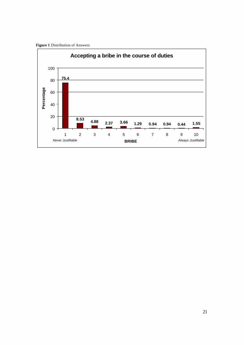
Figure 1 presents the share of responses for each category. While 75.4 percent of indi-

viduals value the acceptance of bribes as an action that is never justifiable, 8.8 percent of

the sample provided a rank of 5 or above thus showing a relatively high propensity to

condone fraudulent behavior. We use the answer to this question as our measure of the

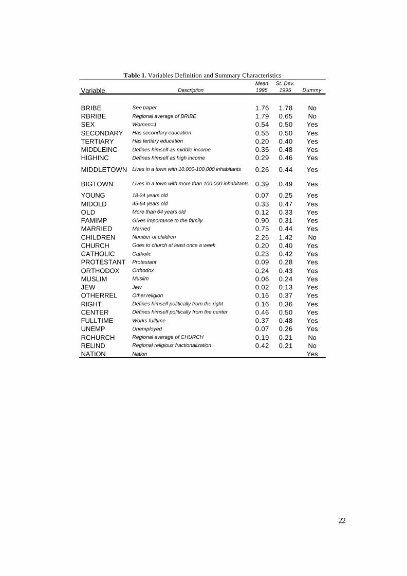
attitude towards corruption. We then regress the individual attitudes towards corruption

(BRIBE) on a set of personal characteristics and values, whose summary characteristics

are presented in Table 1.

Figure 1 Distribution of Answers

Table 1 Variables Definition and Summary Characteristics

Specifically, we first investigate the determinants of individual attitudes towards corrup-

tion without including proxies for social effects, and estimate our specifications using or-

dinary least squares. Since more than 75% percent of individuals value the acceptance of

bribes as an action that is never justifiable (which implies a substantial mass point at

zero), we also performed tobit analyses. However, as results did not change significantly,

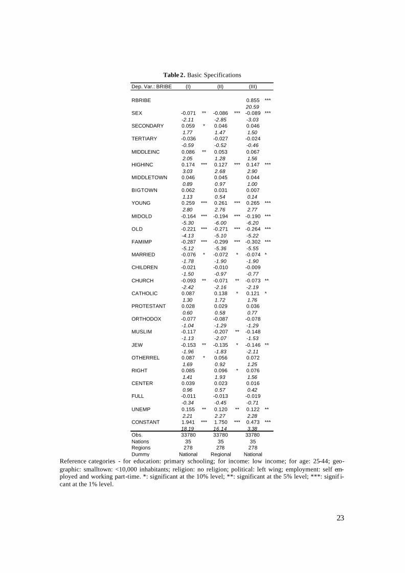
we do not report them here. Estimation results for the basic specification are reported in

Table 2. In column I we control for unobservables by including country fixed effects,

while in column II we instead include regional dummies. We find that the estimates of

personal characteristics are quite robust to the various regression specifications (see the

detailed description below).

8

We then investigate the role of social effects. To do so, we first need to identify ex ante

the reference group that may influence the individual’s perception of corruption (Manski,

1993). In our case, it is likely that the individual’s attitudes towards corruption depend to

a great extent on their interactions with other individuals, as well as on their relation with

the public administration. It seems therefore reasonable to choose as our reference group

the different regions within each country, and proxy for the social effect with the average

of BRIBE within the region where the individual lives (RBRIBE). In addition, the esti-

mation of social effects raise two main methodological concern. The first is the potential

bias of the coefficient estimate due to the presence of unobservables. For exa mple,

RBRIBE could capture the effect of national institutions that are likely to be correlated

with the prevalence of corruption, such as the qua lity of the jurisdictional system. To cor-

rect for this possible bias, we add country fixed effects to the specification. Nevertheless,

a similar problem could also arise at the regional level. Since a regional dummy would be

perfectly collinear with RBRIBE, we address this issue in section V.2 by exploiting time

differences in RBRIBE across two separated waves of the WVS – a first wave conducted

in 1990-93 (Wave II) and a second wave conducted in 1995-97 (Wave III, our main data-

set): time variation in regio nal averages of BRIBE allows us to include regional (time in-

variant) and national (time variant) dummies. Results of this estimation are reported in

Table 3.

The second methodological concern is the identification of social effects. To clarify this

issue, we follow Manski (1993) and write our regression as:

( ) ( ) εγβηα ++++= '||' xzExyEzy

where, in our context, the constant α represents a national dummy capturing the average

attitude towards corruption in the country as well as a host of unobservable country char-

acteristics, x represents the reference group to which the individual belongs (in our case,

the region), z represents personal characteristics, E(y|x) is the average answer of the ref-

erence group (RBRIBE), and E(z|x) represents average characteristics of the reference

9

group (such as, for example, average education in the region). Manski (1993) defines

( ) ( ) γβ '|| xzExyE + as the social effect. More precisely, in Manski’s definition,

( )xyE |β captures the endogenous social effect purely due to peer effects, while

( ) η'| xzE represents the exogenous effect because it depends on the average distribution

of fundamentals.

Manski (1993) shows that, unless additional assumptions are made, it is not possible to

disentangle endogenous and exogenous social effects: in our case, this would mean that

the estimated coefficient on RBRIBE might reflect both the effect of peer interaction as

well as the influence of regional average characteristics on the individual attitudes to-

wards corruption. However, as detailed in the introduction, it remains interesting to verify

whether an overall social effect of either endogenous or exogenous nature affects indi-

viduals’ attitudes towards corruption. To do so, note that, to test whether there are any

social effects, we simply need to run the following regression:

( ) εηβα +++= '| zxyEy

Under the null hypothesis that there are no social effects at all, estimations of the above

regression would deliver insignificant estimates of β. Conversely, we can interpret a sig-

nificant estimate of β as evidence of social e ffects.

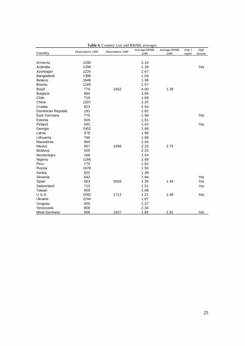
To implement the estimation we proceed as follows. First, we drop all countries that have

only one region, so that only 35 countries are left in the sample (see Table 5). We then

estimate the average ( )xyE i |− for each region (RBRIBE-i), where the answer of individ-

ual i is omitted from the regional average. We then regress the individual response

(BRIBEi) on a country dummy, on personal characteristics, and on the average answer

( )xyE i |− in the region. Results are reported in Table 2, column III, and Table 3, column

II.

Last, we choose not to use the weights provided in the WVS. As we shall see in the next

section, several observations contain missing data. Hence, we perform our multivariate

10

analysis without the use of the existing sampling weights. 4 Consequently, we can not

claim our results to be representative at the national or regional level, but rather circum-

scribed to within sample inference.

IV. Data Description

The data set we use for the analysis is the World Values Survey and European Values

Survey, a cross-country program coordinated by the Institute for Social Research of the

University of Michigan. The series is designed to enable a cross-national comparison on

values and norms on a wide variety of topics. The novelty of the questionnaire is the cov-

erage of a wide array of individual beliefs on politics, religion and economics. It also

provides information on the demographic characteristics of the respondents and their self-

reported economic profile. All surveys were carried out through individual interviews to

adults aged 18 or older. Currently, three waves of the WVS are publicly available (1981-

84, 1990-93, 1995-97). In most specifications we only use data from the 1995-97 wave of

the WVS (Wave III). The third wave of the WVS comprises 55 surveys across 49 coun-

tries for a total of 78,574 individuals interviewed.5 The typical sampling design within

each country is a multi-stage random selection of sampling points after stratification by

region and degree of urbanization.6

As we are ultimately interested in measuring the impact of social effects at the regional

level, we had to restrict the sample in a number of ways. First, we eliminated all country

where the surveys did not contain the variables that are relevant for our analysis (for ex-

ample, information on education was not available for Japan). Second, we excluded from

the sample all surveys conducted on a regional rather than national scale (in Spain, for

4 Nevertheless, we still impose uniform weights on individual observations such that all regions have the same relevance. This is because we analyze social effects at the regional level, so that the relevant observa-tion unit is the region, not the individual. Moreover, as in this case we are not hampered by the missing value problem, in order to guarantee that RBRIBE is representative at the regional level, we used the WVS weights in its computation. 5 Few surveys were also administered at the sub-national level in Puerto Rico, Tabov District, Montenegro, the Andalusian, Basque, Gallician and Valencian regions of Spain, plus a pilot survey in Ghana. However, they were not included in our analysis (see below). 6 For a detailed description of the datasets see Inglehart et al. (2000).

11

instance, in addition to the national survey, four additional regional surveys were con-

ducted). Third, to identify social effects we used as a reference group the regional aver-

ages; hence, we eliminated all the surveys that did not contain any regional identification.

Moreover, in order to guarantee some degree of representativity of the regional averages,

we also excluded all regions with less than forty observations. Finally, a high number of

individual observations were also dropped because of missing data on relevant covariates

(see table 8). After these exclusions, our sample consists of 33,780 observations across 35

countries. In the resulting sample almost 40% of the subjects live in a town with more

than 100,000 inhabitants, 55% of the subjects have secondary education, 29% define

themselves as high income, and 24% are Christian orthodox.

To correct for omitted variable bias at the regional level, we also use data from the 1990-

93 wave (Wave II). Although using the 1990-93 wave allows us to exploit time variations

in the regional averages of individual attitudes towards corruption, there are disadvan-

tages in pooling the two waves together. In particular, Wave II does not include data on

education for most countries, contains a large number of missing observations and also

covers a sample of countries and regions that overlaps only partially with that of Wave

III. Consistent data for our specification were therefore available in both waves for only

36 regions in 5 countries.

V. Empirical Results

V.1 Basic Specification

Table 2 presents the regression estimates for all 35 countries. Note that by including na-

tional (or regional) dummies we implicitly run fixed effect regressions, such that every

estimate has to be interpreted as the deviation with respect to the national (or regional)

average. Relatively few variables are significantly correlated with BRIBE. However,

these correlations are robust across the different regression specifications.

Consistent with the findings of previous studies (Dollar et al., 2001, and Swamy et al.,

2001), women seem to be relatively more averse to corruption (lower BRIBE). We do not

12

find a correlation between the degree of education and corruption, but richer individuals

are more likely to accept some degree of corruption; in particular, this effect is consis-

tently significant for high income people. People also appear to be more averse to corrup-

tion as they age. Moreover, family values and reported church attendance are associated

with higher aversion to corruption. Interestingly, different religious beliefs do not seem to

have a significant impact on BRIBE (with the exception of individuals of Jewish religion

who consistently report a higher aversion to corruption). Finally, we find that unem-

ployed people display less aversion to corruption. Note that the magnitude of the esti-

mated coefficients is not sensitive to whether the fixed effects are computed at the na-

tional or regional level (Table 2, columns I and II).

We then test for the presence of social effects (column III of Table 2). To do so, we sim-

ply regress BRIBE on the regional average RBRIBE without the observations of the sin-

gle individuals, RBRIBE-i, while controlling for personal characteristics. As discussed in

section III, we interpret RBRIBE as a proxy for both endogenous and exogenous social

effects. We consistently find that β̂ is significantly different from zero, indicating that

social effects have overall a significant impact on the individual's perception of corrup-

tion. Moreover, the magnitude of the effect is sizeable – a one-standard deviation in-

crease in RBRIBE is associated with an increase of 30% of a standard deviation in the

individual attitude towards corruption. Note that the estimates of personal characteristics

are quite robust across all regressions, even after including the social effect.

Table 2. Basic specification regressions

V. 2 High vs. Low and Middle Income Countries

Empirical evidence tends to support the idea that, overall, corruption is assoc iated with

low economic performance (see, for instance, the reviews of Bardhan, 1997, and Tanzi,

1998). For example, the correlation between the index of absence of corruption devel-

oped by Transparency International (2002) and real GDP per capita is 0.88.7 Similarly,

7 The corruption index of Transparency International varies from one to ten, where more corrupted coun-tries obtain a lower score.

13

across the 35 countries in our dataset higher corruption is associated with lower levels of

development (correlation of -0.3). In particular, 73.3% of the respondents in developing

countries consider accepting a bribe as ne ver justifiable, while the percentage rises to

84.6% in more developed countries. In this context, it is interesting to investigate whether

individuals residing in low/high income countries display structural differences with re-

gards to their attitudes towards corruption. 8 To do so we run our basic regression as in

Table 2 for individuals in low and high income countries separately, and then test for

model equivalence. Interestingly, we obtain that individuals’ behavior is independent

from the level of development of the country of residence.9 In other words, despite the

difference in average responses reported above, individual characteristics and social ef-

fects appear to affect the perception of corruption in the same fashion both in low and

high income countries.

8 Low/high income countries are defined here as countries with GDP per capita below/above 9000 US $ in 1995. 9 The results of the Chow tests performed are F(24,33697)=1.48 for regression (I), F(24,33454)=0.81 for regression (II), and F(25,33695)=1.24 for regression (III). Therefore, we can not reject the null hypothesis that the two models are equivalent.

14

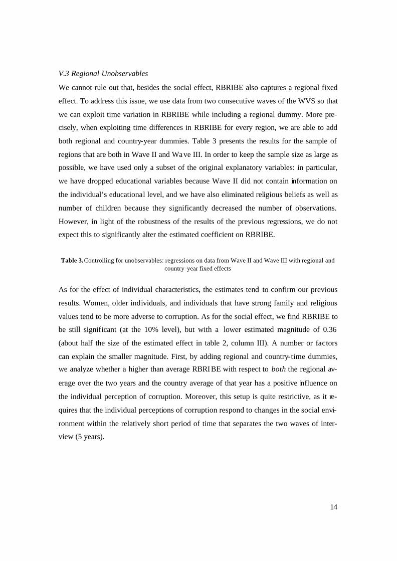
V.3 Regional Unobservables

We cannot rule out that, besides the social effect, RBRIBE also captures a regional fixed

effect. To address this issue, we use data from two consecutive waves of the WVS so that

we can exploit time variation in RBRIBE while including a regional dummy. More pre-

cisely, when exploiting time differences in RBRIBE for every region, we are able to add

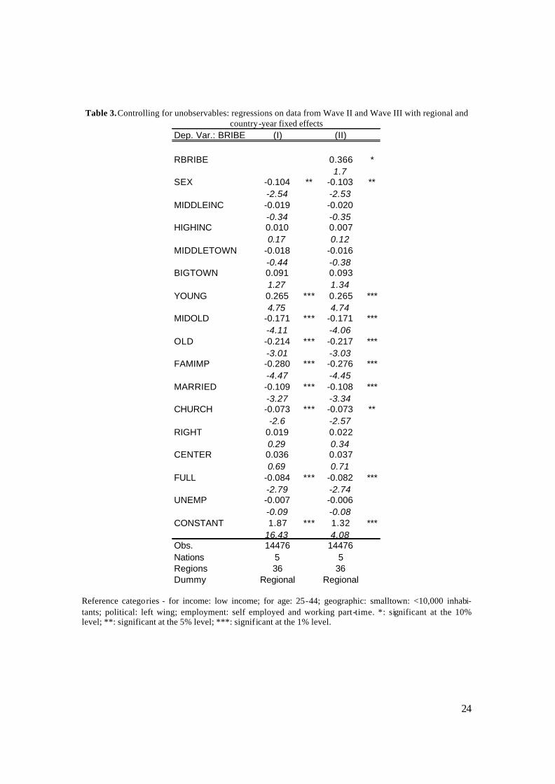
both regional and country-year dummies. Table 3 presents the results for the sample of

regions that are both in Wave II and Wave III. In order to keep the sample size as large as

possible, we have used only a subset of the original explanatory variables: in particular,

we have dropped educational variables because Wave II did not contain information on

the individual’s educational level, and we have also eliminated religious beliefs as well as

number of children because they significantly decreased the number of observations.

However, in light of the robustness of the results of the previous regressions, we do not

expect this to significantly alter the estimated coefficient on RBRIBE.

Table 3. Controlling for unobservables: regressions on data from Wave II and Wave III with regional and country-year fixed effects

As for the effect of individual characteristics, the estimates tend to confirm our previous

results. Women, older individuals, and individuals that have strong family and religious

values tend to be more adverse to corruption. As for the social effect, we find RBRIBE to

be still significant (at the 10% level), but with a lower estimated magnitude of 0.36

(about half the size of the estimated effect in table 2, column III). A number or factors

can explain the smaller magnitude. First, by adding regional and country-time dummies,

we analyze whether a higher than average RBRIBE with respect to both the regional av-

erage over the two years and the country average of that year has a positive influence on

the individual perception of corruption. Moreover, this setup is quite restrictive, as it re-

quires that the individual perceptions of corruption respond to changes in the social envi-

ronment within the relatively short period of time that separates the two waves of inter-

view (5 years).

15

VI. Conclusions

Although issues of governance and corruption have been recently at the center of the aca-

demic and policymaking debates, the literature documenting the determinants of corrup-

tion at the microeconomic level is scant. This paper attempts to fill this gap in two dis-

tinct directions. First, using data from the World Value Survey, a large dataset contain-

ing, amongst others, information on personal attitudes towards corruption in more than 50

countries of the developed and developing world, we consistently find that women, em-

ployed, less wealthy, and older individuals report to be more averse to corruption. Sec-

ond, we investigate the extent to which the social environment influences individual atti-

tudes towards corruption. We find that, ceteris paribus, individuals tend to be more for-

giving of corruption in regions where, on average, people are relatively less averse to it.

Moreover, the social effect seems to be of sizeable magnitude. This suggests that the in-

dividual incentives to oppose corruption might be low, and that an effective fight against

corruption may need to be a coordinated “big push” operating on several fronts at once.

16

References

Ades, Alberto and Rafael Di Tella (1999). “Rents, Competition, and Corruption,” Ameri-

can Economic Review, 89(4), 982-93.

Andvig, Jens C. and Karl O. Moene (1990). “How Corruption May Corrupt,” Journal of

Economic Behavior and Organization, 13, 63-76.

Banerjee, Abhijit (1997). “A Theory of Misgovernance,” Quarterly Journal of Econom-

ics, 112(4), 1289-1332.

Bardhan, Pranab (1997). “Corruption and Development: A Review of Issues,” Journal of

Economic Literature, 35(3), 1320-46.

Baumol, William J (1990). “Entrepreneurship: Productive, Unproductive, and Destruc-

tive,” Journal of Political Economy, 98, 893-921.

Beck, Paul J and Michael W Maher (1986). “A Comparison of Bribery and Bidding in

Thin Markets,” Economics Letters, 20(1), 1-5.

Becker, Gary and George J. Stigler (1974). “Law Enforcement, Malfeasance, and the

Compensation of Enforcers,” Journal of Legal Studies, III, 1-19

Bertrand, Marianne, Erzo F. P. Luttmer and Sendhil Mullainathan (2000). “Network Ef-

fects and Welfare Cultures,” The Quarterly Journal of Economics, 115(3), 1019-55.

Borjas, Geroge J. (1992). “Ethnic Capital and Intergenerational Mobility,” The Quarterly

Journal of Economics, 107, 123-50.

17

------ (1994). “Long-Run Convergence of Ethnic Skill Differentials: The Children and

Grandchildren of the Great Migration,” Industrial and Labor Relations Review, 47, 553-

73.

Braun, Miguel, and Rafael di Tella (2002). “Inflation and Corruption,” Harvard Business

School, mimeo.

Cadot, Oliver (1987). “Corruption as a Gamble,” Journal of Public Economics, 33, 223-

44.

Case, Anne and Lawrence Katz (1991). “The Company You Keep: The Effects of Family

and Neighborhood on Disadvantaged Youths,” NBER Working Paper 3705.

Collier, Paul (1999). “How to Reduce Corruption,” Manuscript, The World Bank.

Dollar, David, Raymond Fisman and Roberta Gatti (2001). “Are Women Really the

"Fairer" Sex? Corruption and Women in Government,” Journal of Economic Behavior

and Organization, 46(4), 423-29.

Fisman, Raymond and Roberta Gatti (2002). “Decentralization and Corruption: Evidence

across Countries,” Journal of Public Economics, 83(3), 325-45.

Glaeser, Edward L, Bruce Sacerdote and José A Scheinkman (1996). “Crime and Social

Interactions,” The Quarterly Journal of Economics, 111, 507-48.

Guiso, Luigi, Paola Sapienza and Luigi Zingales (2002). “People’s Opium? Religion and

Economic Att itudes,” mimeo.

Huntington, Samuel (1968). Political Order in Changing Societies, Yale University

Press, New Haven.

18

Ichino, Andrea, and Giovanni Maggi (2000). “Work Environment and Individual Back-

ground: Explaining Regional Shirking Differentials in a Large Italian Firm,” The Quar-

terly Journal of Economics, 115(3), 1057-90.

Inglehart, Ronald et Al. (2000). “World Value Surveys and European Value Surveys,

1981-1984, 1990-1993, 1995-1997,” ICPSR 2790, University of Michigan.

Katz, Lawrence F, Jeffrey R Kling and Jeffrey B Liebman (2001). “Moving to Opportu-

nity in Boston: Early Result of a Randomized Mobility Experiment,” The Quarterly Jour-

nal of Economics, 116(2), 607-54.

Knack, Steven and Philip Keefer (1997). “Does Social Capital Have an Economic Pay-

off? A Cross-Country Investigation,” The Quarterly Journal of Economics, 112(4), 1251-

88.

Krueger, Anne (1974). “The Political Economy of the Rent-Seeking Society,” The

American Economic Review, 64, 291-303.

Leff, Nathaniel, “Economic Development through Bureaucratic Corruption,” American

Behavioral Scientist, 8-14.

Lien, Da Hsiang Donald (1986). “A Note on Competitive Bribery Games,” Economics

Letters, 22(4), 337-41.

Ludwig, Jens, Greg J Duncan and Paul Hirshfeld (2001). “Urban Poverty and Juvenile

Crime: Evidence from a Randomized Housing-Mobility Experiment,” The Quarterly

Journal of Economics, 116, 655-79.

MacCulloch, Robert and Silvia Pezzini (2002). “Pricing Freedom with Revolutionary

Preferences of Christians and Muslims,” mimeo, London School of Economics.

19

Manski, Charles F (1993). “Identification of Endogenous Social Effects: The Reflection

Problem,” Review of Economic Studies, 60, 531-42.

Mauro, Paolo (1995). “Corruption and Growth,” The Quarterly Journal of Economics,

110(3), 681-712.

------- (1997). “Corruption and the Composition of Government Expenditure,” Journal of

Public Economics, 69, 263-79.

Murphy, Kevin M, Andrei Shleifer and Robert W Vishny (1989). “Industrialization and

The Big Push,” The Journal of Political Economy , 97(5), 1003-26.

------ (1991). “The Allocation of Ta lent: Implication for Growth,” The Quarterly Journal

of Economics, 106, 503-30.

Paternostro, Stefano (1997) “The Poverty Trap: The Dual Externality Model and Its Pol-

icy Implications,” World Development, 25 (12), 2071-81.

Rose-Ackerman, Susan (1978). Corruption: A Study of Political Economy, New York,

Academic Press.

Rosenstein-Rodan, Paul (1943). “Problems of Industrialization of Eastern and South-

Eastern Europe,” Economic Journal, 53, 202-11.

Sacerdote, Bruce (2001). “Peer Effects with Random Assignment: Results for Dartmouth

Roommates,” The Quarterly Journal of Economics, 116(2), 681-704.

Shleifer Andrei and Vishny Robert (1993). “Corruption,” Quarterly Journal of Econom-

ics, 108, 599-617.

20

Swamy, Anand, Stephen Knack, Young Lee and Omar Azfar (2001). “Gender and Cor-

ruption,” Journal of Development Economics, 64, 25-55.

Tanzi, Vito (1998). “Corruption Around the World: Causes, Consequences, Scope, and

Cures,” IMF Staff Papers, 45, 559-94.

Tirole, Jean (1996). “A Theory of Collective Reputations (with Applications to the Per-

sistence of Corruption and to Firm Quality)” The Review of Economic Studies, 63(1), 1-

22.

Topa, Giorgio (2001). “Social Interactions, Local Spillovers and Unemployment,” Re-

view of Economic Studies, 68, 261-295.

Transparency International (2002). Global Corruption Report 2002,

www.transparency.org.

Treisman, Daniel (2000). “The Causes of Corruption: A Cross-National Study,” Journal

of Public Economics, 76(3), 399-457.

21

Figure 1 Distribution of Answers

Accepting a bribe in the course of duties

8.534.88 2.37 3.66 1.29 0.94 0.94 0.44 1.55

75.4

0

20

40

60

80

100

1 2 3 4 5 6 7 8 9 10

BRIBE

Per

cen

tag

e

Never Justifiable Always Justifiable

22

Table 1. Variables Definition and Summary Characteristics

Variable DescriptionMean 1995

St. Dev. 1995 Dummy

BRIBE See paper 1.76 1.78 NoRBRIBE Regional average of BRIBE 1.79 0.65 NoSEX Women=1 0.54 0.50 YesSECONDARY Has secondary education 0.55 0.50 YesTERTIARY Has tertiary education 0.20 0.40 YesMIDDLEINC Defines himself as middle income 0.35 0.48 YesHIGHINC Defines himself as high income 0.29 0.46 Yes

MIDDLETOWN Lives in a town with 10.000-100.000 inhabitants 0.26 0.44 Yes

BIGTOWN Lives in a town with more than 100.000 inhabitants 0.39 0.49 Yes

YOUNG 18-24 years old 0.07 0.25 YesMIDOLD 45-64 years old 0.33 0.47 YesOLD More than 64 years old 0.12 0.33 YesFAMIMP Gives importance to the family 0.90 0.31 YesMARRIED Married 0.75 0.44 YesCHILDREN Number of children 2.26 1.42 NoCHURCH Goes to church at least once a week 0.20 0.40 YesCATHOLIC Catholic 0.23 0.42 YesPROTESTANT Protestant 0.09 0.28 YesORTHODOX Orthodox 0.24 0.43 YesMUSLIM Muslim 0.06 0.24 YesJEW Jew 0.02 0.13 YesOTHERREL Other religion 0.16 0.37 YesRIGHT Defines himself politically from the right 0.16 0.36 YesCENTER Defines himself politically from the center 0.46 0.50 YesFULLTIME Works fulltime 0.37 0.48 YesUNEMP Unemployed 0.07 0.26 YesRCHURCH Regional average of CHURCH 0.19 0.21 NoRELIND Regional religious fractionalization 0.42 0.21 NoNATION Nation Yes

23

Table 2. Basic Specifications

Reference categories - for education: primary schooling; for income: low income; for age: 25-44; geo-graphic: smalltown: <10,000 inhabitants; religion: no religion; political: left wing; employment: self em-ployed and working part-time. *: significant at the 10% level; **: significant at the 5% level; ***: signif i-cant at the 1% level.

Dep. Var.: BRIBE (I) (II) (III)

RBRIBE 0.855 ***20.59

SEX -0.071 ** -0.086 *** -0.089 ***-2.11 -2.85 -3.03

SECONDARY 0.059 * 0.046 0.0461.77 1.47 1.50

TERTIARY -0.036 -0.027 -0.024-0.59 -0.52 -0.46

MIDDLEINC 0.086 ** 0.053 0.0672.05 1.28 1.56

HIGHINC 0.174 *** 0.127 *** 0.147 ***3.03 2.68 2.90

MIDDLETOWN 0.046 0.045 0.0440.89 0.97 1.00

BIGTOWN 0.062 0.031 0.0071.13 0.54 0.14

YOUNG 0.259 *** 0.261 *** 0.265 ***2.80 2.76 2.77

MIDOLD -0.164 *** -0.194 *** -0.190 ***-5.30 -6.00 -6.20

OLD -0.221 *** -0.271 *** -0.264 ***-4.13 -5.10 -5.22

FAMIMP -0.287 *** -0.299 *** -0.302 ***-5.12 -5.36 -5.55

MARRIED -0.076 * -0.072 * -0.074 *-1.78 -1.90 -1.90

CHILDREN -0.021 -0.010 -0.009-1.50 -0.97 -0.77

CHURCH -0.093 ** -0.071 ** -0.073 **-2.42 -2.16 -2.19

CATHOLIC 0.087 0.138 * 0.121 *1.30 1.72 1.76

PROTESTANT 0.028 0.029 0.0360.60 0.58 0.77

ORTHODOX -0.077 -0.087 -0.078-1.04 -1.29 -1.29

MUSLIM -0.117 -0.207 ** -0.148-1.13 -2.07 -1.53

JEW -0.153 ** -0.135 * -0.146 **-1.96 -1.83 -2.11

OTHERREL 0.087 * 0.056 0.0721.69 0.92 1.25

RIGHT 0.085 0.096 * 0.0761.41 1.93 1.56

CENTER 0.039 0.023 0.0160.96 0.57 0.42

FULL -0.011 -0.013 -0.019-0.34 -0.45 -0.71

UNEMP 0.155 ** 0.120 ** 0.122 **2.21 2.27 2.28

CONSTANT 1.941 *** 1.750 *** 0.473 ***18.19 16.14 3.38

Obs. 33780 33780 33780Nations 35 35 35Regions 278 278 278Dummy National Regional National

24

Table 3. Controlling for unobservables: regressions on data from Wave II and Wave III with regional and

country-year fixed effects

Reference categories - for income: low income; for age: 25-44; geographic: smalltown: <10,000 inhabi-tants; political: left wing; employment: self employed and working part-time. *: significant at the 10% level; **: significant at the 5% level; ***: significant at the 1% level.

Dep. Var.: BRIBE (I) (II)

RBRIBE 0.366 *1.7

SEX -0.104 ** -0.103 **-2.54 -2.53

MIDDLEINC -0.019 -0.020-0.34 -0.35

HIGHINC 0.010 0.0070.17 0.12

MIDDLETOWN -0.018 -0.016-0.44 -0.38

BIGTOWN 0.091 0.0931.27 1.34

YOUNG 0.265 *** 0.265 ***4.75 4.74

MIDOLD -0.171 *** -0.171 ***-4.11 -4.06

OLD -0.214 *** -0.217 ***-3.01 -3.03

FAMIMP -0.280 *** -0.276 ***-4.47 -4.45

MARRIED -0.109 *** -0.108 ***-3.27 -3.34

CHURCH -0.073 *** -0.073 **-2.6 -2.57

RIGHT 0.019 0.0220.29 0.34

CENTER 0.036 0.0370.69 0.71

FULL -0.084 *** -0.082 ***-2.79 -2.74

UNEMP -0.007 -0.006-0.09 -0.08

CONSTANT 1.87 *** 1.32 ***16.43 4.08

Obs. 14476 14476Nations 5 5Regions 36 36Dummy Regional Regional

25

Table 4. Country List and BRIBE averages

Country Observations 1995 Observations 1990Average BRIBE

1995Average BRIBE

1990Only 1 region

High Income

Armenia 1290 2.10Australia 1299 1.28 YesAzerbaijan 1220 2.67Bangladesh 1388 1.03Belarus 1648 1.98Bosnia 1165 1.57Brazil 770 1662 4.00 1.39Bulgaria 984 1.89Chile 719 1.68China 1207 1.20Croatia 823 2.04Dominican Republic 181 1.82East Germany 775 1.99 YesEstonia 609 1.51Finland 592 1.42 YesGeorgia 2452 1.88Latvia 378 1.98Lithuania 766 1.89Macedonia 960 1.40Mexico 957 1486 2.33 2.75Moldova 559 2.25Montenegro 168 1.54Nigeria 1166 1.89Peru 770 1.62Russia 1678 1.50Serbia 922 1.38Slovenia 642 1.84 YesSpain 663 3556 1.36 1.49 YesSwitzerland 713 1.51 YesTaiwan 909 1.68U.S.A. 1092 1712 1.21 1.48 YesUkraine 2244 1.87Uruguay 655 1.27Venezuela 858 2.34West Germany 558 1937 1.82 1.91 Yes