Embed Size (px)
Citation preview
Industry Connections and the Geographic Location of
Economic Activity∗
W. Walker Hanlon
PhD Candidate, Department of Economics, Columbia University
PRELIMINARY DRAFT
June 15, 2011
Abstract
This paper provides causal evidence that inter-industry connections can influencethe geographic location of economic activity. To do so, it takes advantage of a large,exogenous, temporary, and industry-specific shock to the 19th century British economy.The shock was caused by the U.S. Civil War, which sharply reduced raw cotton suppliesto Britain’s important cotton textile industry, causing a four year recession in the in-dustry. The impact of the shock on towns in Lancashire County, the center of Britain’scotton textile industry, is compared to towns in neighboring Yorkshire County, wherewool textiles dominated. The results suggest that this trade shock reduced employmentand employment growth in industries related to the cotton textile industry, in townsthat were more severely impacted by the shock, relative to less affected towns. Theimpact still appears over two decades after the end of the U.S. Civil War. This suggeststhat temporary shocks, acting through inter-industry connections, can have long-termimpacts on the distribution of industrial activity across locations.
∗This paper benefited enormously from the input of Don Davis and Eric Verhoogen. Thanks also to
Ronald Findlay, Amit Khandelwal, Jonathan Vogel, David Weinstein, Guy Michaels, Henry Overman,
Richard Hornbeck, William Kerr, Ryan Chahrour, and participants in the Columbia International Trade
Colloquium and Manchester Graduate Summer School. Thanks to Matthew Wollard and Ole Wiedenmann
at the UK Data Archive, who provided help with the data used in this project, and to Tim Leunig and
Humphrey Southall for help understanding this period in economic history. Funding for this project was
provided by the National Science Foundation (grant no. 0962545) and the Economic History Association.
1
1 Introduction
Marshall (1890) suggested that firms in different industries may benefit from locating nearto one another, through localized inter-industry spillovers. He identified three channelsthrough which these benefits could flow: input-output linkages, labor market pooling, ortechnology spillovers. Since then, inter-industry spillovers have been incorporated into the-ories of industrial linkages and development (Hirschman (1958), Ciccone (2007)), industrialclusters (Porter (1990)), the benefits of urban economies (Jacobs (1969)), the benefits oftrade and FDI (Young (1991), Rodrıguez-Clare (1996)), and the geography of economicactivity (Krugman & Venables (1995)). Policy makers, too, have been influenced by theseideas. The existence of inter-industry spillovers is one of the prime motivations for localindustrial policies, such as the tax incentives offered to firms by U.S. municipalities, or thewidespread use of special industrial zones in developing countries. The cost of these policiescan run into the hundreds of millions of dollars for single U.S. municipalities.1
Despite this interest, and widespread application, empirical evidence on the role of inter-industry connections in influencing the geographic location of economic activity is sparse.This is due largely to the difficulty of measuring the patterns of connections between indus-tries, though these measures are improving.2 In an important recent study, Greenstone et al.(2010) show evidence of localized productivity spillovers between plants that share similarlabor or technology pools.3 In a similar vein, Javorcik (2004) finds evidence of spilloversfrom FDI firms to upstream suppliers.4 More related to the current study is Ellison et al.(2010), which uses measures of input-output connections, labor force similarity, and tech-nological spillovers, to provide evidence that the underlying pattern of connections betweenindustries is influencing the geographic location of industries. While these are importantcontributions, they do not address the most relevant question for policy: can temporarychanges in the local availability of inter-industry spillovers, such as those created by eco-nomic shocks or policy interventions, have long-term impacts on the geographic location ofeconomic activity?
This study takes the next step, by utilizing a large temporary external shock thataltered the spillovers available to certain industries in certain locations, in order to providecausal evidence that changes in the availability of inter-industry spillovers can influence
1See Greenstone & Moretti (2004).2There are a number of early studies which looked for the impact of inter-industry connections without ac-
counting for the patterns that these connections take. Important contributions include Glaeser et al. (1992),
Kim (1995), Henderson (1997), and Henderson (2003). There is also a much larger literature considering
the role of spillovers within industries.3Another interesting contribution is Bloom et al. (2007).4Similar evidence is also provided by Kugler (2006), Poole (2009), and Balsvik (Forthcoming).
2
the long-run distribution of economic activity. The shock was caused by the U.S. CivilWar and impacted the British economy in the 1860s. During the 19th century, cottontextile production was the largest British manufacturing industry, and cotton textiles wereBritain’s largest export. This industry relied entirely on imports of raw cotton, a vitalinput. Prior to the onset of the U.S. Civil War in 1861, the majority of raw cotton camefrom the Southern U.S., but the war, and the corresponding Union blockade of Southernports, sharply reduced raw cotton supplies. The result was a four year depression in theindustry, lasting from roughly 1861-1865. Our focus will be on how this affected the locationof those industries related to (sharing spillovers with) the cotton textile industry.
As with other studies using historical examples (e.g., Donaldson (2010)), the eventconsidered in this study was chosen because it has features that are particularly helpful inidentifying the effects of interest, which are unlikely to be found in similar modern events.First, the shock was large, exogenous, and temporary. While the cotton shortage reducedproduction by about half during the shock period, the cotton textile industry reboundedquickly, attaining its original growth path by roughly 1866-67, only a year or two afterthe end of the war. Second, the direct effects of the shock were largely industry-specific.British import and export data suggest that, once cotton textiles are removed, the shock hadno major effect on other British manufacturing sectors. Thus, changes observed in thoseindustries related to cotton textiles can be attributed to the shock, transmitted throughinter-industry connections. Third, despite the large magnitude of the negative effects of thecotton shortage, there was virtually no government intervention. This was largely due tothe very strong free-market ideology that was dominant in Britain at the time, particularlyin the northern industrial districts that were hardest hit by the recession.
A final important feature is that some locations were severely impacted, while other,economically similar locations, were left nearly untouched. This study compares outcomesin towns from two industrial counties in the north of England, Lancashire and Yorkshire.Lancashire was the heart of Britain’s cotton textile industry at the time. Yorkshire, lyingjust to the east, was similar to Lancashire in many ways. The key difference betweenthese two counties was that, while towns in Yorkshire also had large textile industries,Yorkshire producers focused primarily on wool-based textiles (woollens & worsted) ratherthan cotton. Thus, while towns in Lancashire were severely affected by the cotton shortage,towns in Yorkshire were not negatively impacted. Comparing industry growth rates fromtowns in these two counties thus allows us to better identify the impact of the shock.
The basic hypothesis that we test is that the shock negatively affected employmentand employment growth in industries more closely related to the cotton textile industry, inlocations more severely impacted by the shock, by reducing the spillover benefits available tothese industries. Importantly, we focus on impacts occurring in the years and decades after
3
the Civil War had ended and the cotton textile industry had rebounded. The hypothesisis motivated by a two-country dynamic Ricardian trade model building on work by Young(1991) and Matsuyama (1992). In the model, technology growth is driven by localizedlearning-by-doing spillovers within and between industries. A negative shock to one industryreduces the spillover benefits enjoyed by related industries, in the location in which theaffected industry is concentrated. The result is a reduction in technology growth in therelated industry, in the more severely affected location relative to the less affected location.Moreover, the model describes channels through which a loss of spillovers in one periodcan affect employment and employment growth in related industries in future periods. Themodel is used to derive the empirical specification used in the analysis.
This intuition is perhaps best illustrated using an example from the empirical setting,provided by the Engine & Machinery industry (E&M). This was an important industry inBritain at this time, and one that was connected to the cotton textile industry in Lancashire,as well as the wool textile industry in Yorkshire, through all three of Marshall’s channels. Infact, Marshall himself used the textile and engineering industries to illustrate the possibilityof labor market pooling benefits.5 There is also evidence suggesting that textile machinemakers learned from the nearby textile producers that they supplied. Engine and machinemakers in Lancashire and Yorkshire competed, both to supply customers in these locations,as well as in the important export market. The data show that the E&M industry had asimilar growth path in the two locations prior to the shock, but that E&M firms in York-shire towns gained an advantage relative to Lancashire producers in the following decades,allowing them to expand employment more rapidly. This suggests that the recession in thecotton textile industry had persistent impacts on distribution of the E&M industry acrosslocations.
The empirical strategy used to test this hypothesis involves using panel data with twocross-sectional dimension, allowing us to compare impacts across time (pre vs. post shockperiods), locations (towns with higher vs. lower shock intensity), and industries (more vs.less related to cotton textiles). The primary data are drawn from the British Census ofProduction, which were gathered from original sources. These data provide employmentdisaggregated into 171 industry groups, spanning nearly the entire private sector economy,available for every ten years from 1851-1891. Thus, we have multiple observations in boththe pre- and post-shock period, and are able to observe effects up to 25 years after the endof the recession. These data are available for 11 principal towns, 6 in Lancashire, and 5 inYorkshire, providing the geographic dimension of the analysis. Additional data from localPoor Law boards, which were the primary source of funds for unemployed workers duringthis period, allow us to measure the severity of the shock in each town. We find that the
5Marshall (1920) (p. 226).
4
share of cotton textiles in a town’s employment in 1851 is a good predictor of the severityof the shock in each location. Thus we are able to strengthen our identification strategy byusing each town’s cotton textile employment in 1851 as an instrument for shock intensity.
An important input into the analysis is a measure of the pattern of connections betweenthe cotton textile industry and other industries. Two measures are used. The first is basedon the degree to which each industry is geographically coagglomerated with the cottontextile industry, following work by Ellison & Glaeser (1997). Ellison et al. (2010) showthat this measure is related to measures of input-output linkages, labor market poolingpotential, and technology spillovers. The second measure is an intermediate goods input-output matrix based on Thomas (1987).
The results suggest that industries more closely related to the cotton textile industry,based on the geographic coagglomeration measure, suffered lower employment and employ-ment growth, in more severely affected towns, in the post shock period. The impacts areestimated while controlling for aggregate industry-level and town-level shocks in each year,as well as time-invariant industry-location factors. The impact of the shock on employmentand employment growth continues to appear through the 1881-1891 period. The implica-tion is that inter-industry connections can play an important role in affecting the geographiclocation of economic activity across locations. Moreover, temporary changes in the avail-ability of these connections appear to have the potential to generate long-lasting effects.There appear to be no persistent effects related to the intermediate goods input-output ma-trix, suggesting that the observed effects are being driven by other types of inter-industryconnections.
This project is related to three additional strands of literature. On set of related litera-ture studies whether temporary shocks have long-term impacts on the geographic locationof economic activity, in order to to test economic geography models which predict multipleequilibria in the location of economic activity.6 Most studies focus on the impact of tem-porary shocks caused by war on city size.7 Only two studies consider the impact on thelocation of industries, and these deliver mixed results.8 This study improves on previouswork by (1) considering the role of industry connections and (2) using data that are more
6See, e.g., Krugman (1991), Krugman & Venables (1995), Fujita et al. (1999).7Davis & Weinstein (2002), Brakman et al. (2004), Bosker et al. (2007), Bosker et al. (2008b), and Bosker
et al. (2008a). In related work, Miguel & Roland (2006) consider the impact of bombing in Vietnam on
welfare outcomes.8Davis & Weinstein (2008) study the effect of the WWII bombing of Japanese cities on the location of
eight highly aggregated industrial sectors (e.g., machinery, metals) and find no evidence of persistent effects.
In contrast, Redding et al. (forthcoming) study the impact of the division of Germany following WWII on
one particular industry, airport hubs, and find evidence of a persistent effect.
5
detailed and comprehensive.9 The results of this study are consistent with the existenceof multiple equilibria in the geographic location of economic activity, providing support foreconomic geography models predicting multiple equilibria.
Second, because this project considers the impact of a large temporary trade shock onindustry growth over a relatively long time frame, it can help inform our understandingof the relationship between trade and growth. While there is a large empirical literaturestudying the overall relationship between trade and growth, there are relatively few studiesconsidering the impacts of temporary trade shocks.10 The contribution of this study is toshow that temporary trade shocks can have long-term economic impacts. Moreover, whilewe have focused on two regions with a country, in order to better identify the effects ofinterest, our results raise the possibility that trade shocks may also result in reallocationsof industries across countries, which could have long-term impacts on country growth ratesand the gains from trade. This suggests that a complete understanding of the relationshipbetween trade and growth should take into account the potential effects of increased (ordecreased) susceptibility to trade shocks, in addition to the more direct effects of increasedoverall trade.11
Finally, because we study the textile industry in 19th century Britain, there is a naturalconnection to the debate over the sources of the Industrial Revolution. In particular, thereis disagreement over the importance of trade in generating British economic growth.12 Theresults of this study support the view, due to Allen (2009) and others, that trade propelledtechnological progress in the engineering and machinery industries, primary drivers of theindustrial revolution, through their connections with the large textile industries.13
The next section provides background information on the empirical setting and describesthe shock, while Section 3 describes the data used. Section 4 studies the impact on oneindustry, Engine & Machine manufacturing. Section 5 introduces a model that is used toguide the econometric analysis, which is presented in Section 6. Section 7 concludes.
9For example, this study considers 171 industry groups, while Davis & Weinstein (2008) consider only
eight aggregated industrial sectors and Redding et al. (forthcoming) consider only one, airport hubs.10See Rodriguez & Rodrik (2000) for a review and critique of recent macroeconomic literature on trade
and growth.11Recent work by di Giovanni & Levchenko (2009) suggests that trade liberalization may increase volatility
in an economy.12Authors such as Deane & Cole (1967) and Rostow (1960) emphasized that trade, by generating the
demand which allowed the expansion of the cotton textile industry, was a key “engine of growth”. Mokyr
(1985) (p. 22) and McCloskey (1994) (p. 255-258) have disputed this view, arguing that trade, while helpful,
did not drive productivity growth, and that gains from trade were relatively small.13Among the most related industries to cotton textiles, based on the geographic coagglomeration mea-
sure, are “Engineering and Machinery”, “Millwrights”, and “Iron and Steel”. This argument is made for
industrialization more generally by Ciccone (2002).
6
2 Empirical setting
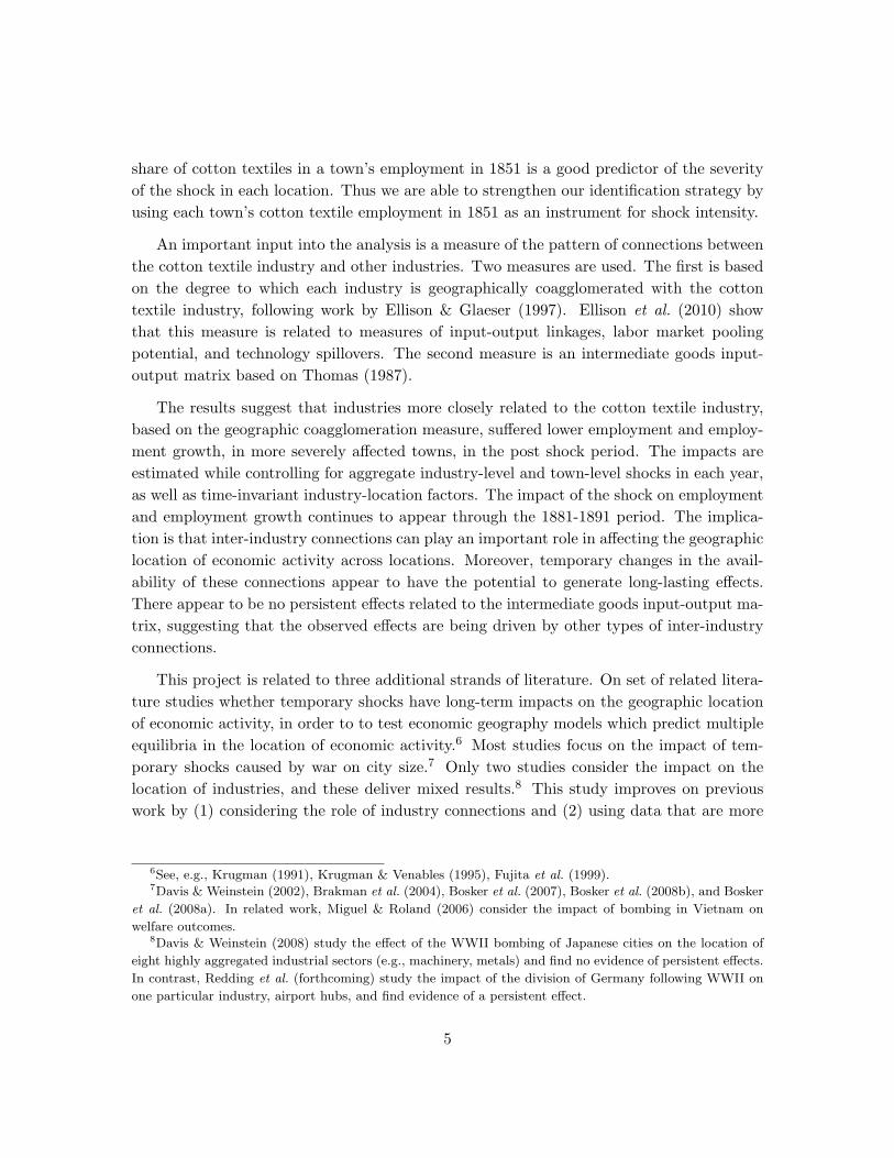
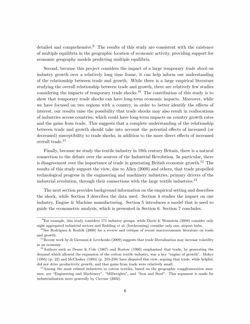
Lancashire County, in the Northwest of England, was the heart of the British cotton textileindustry from the end of the 18th century and the cradle of the Industrial Revolution. Forthe purposes of this study, Cheshire, a smaller cotton textile producing county just south ofLancashire, is treated as part of Lancashire. Lancashire’s main commercial city, Manchester,became synonymous with the cotton textile trade, and the main port, Liverpool, served asthe center of the world’s raw cotton market. Yorkshire, the large and historically importantcounty just east of Lancashire had followed Lancashire’s lead in industrialization and wassimilar to Lancashire in many respects. This study focuses only on the West Riding area ofYorkshire, which is the main industrial area of the county.14 Figure 1 shows the location ofthese counties in England (left panel) and highlights the principal towns (right panel), overwhich the analysis will be conducted. Figure 2 shows that, while Lancashire was somewhatlarger than Yorkshire during the study period, the two counties followed similar populationgrowth paths and had relatively similar industrial structures.
Figure 1: Maps of the study area
Map of English Counties in 1851 Map of Northwestern England and the West Riding
14This practice is common for historians studying Yorkshire during this period, because it separates the
more modern industrial area of the West Riding from the less developed economies of the North and East
Riding.
7
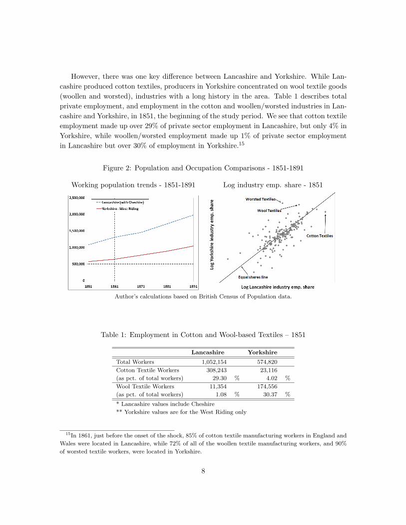
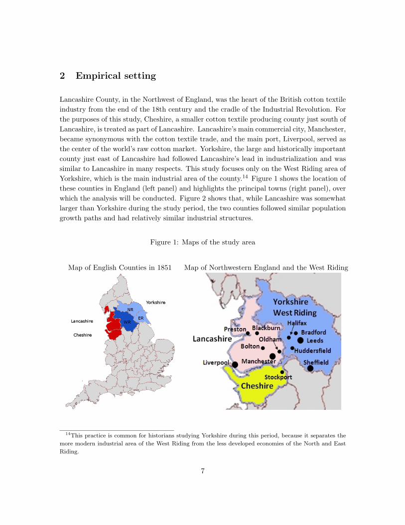
However, there was one key difference between Lancashire and Yorkshire. While Lan-cashire produced cotton textiles, producers in Yorkshire concentrated on wool textile goods(woollen and worsted), industries with a long history in the area. Table 1 describes totalprivate employment, and employment in the cotton and woollen/worsted industries in Lan-cashire and Yorkshire, in 1851, the beginning of the study period. We see that cotton textileemployment made up over 29% of private sector employment in Lancashire, but only 4% inYorkshire, while woollen/worsted employment made up 1% of private sector employmentin Lancashire but over 30% of employment in Yorkshire.15
Figure 2: Population and Occupation Comparisons - 1851-1891
Working population trends - 1851-1891 Log industry emp. share - 1851
Author’s calculations based on British Census of Population data.
Table 1: Employment in Cotton and Wool-based Textiles – 1851
Lancashire Yorkshire
Total Workers 1,052,154 574,820
Cotton Textile Workers 308,243 23,116
(as pct. of total workers) 29.30 % 4.02 %
Wool Textile Workers 11,354 174,556
(as pct. of total workers) 1.08 % 30.37 %
* Lancashire values include Cheshire
** Yorkshire values are for the West Riding only
15In 1861, just before the onset of the shock, 85% of cotton textile manufacturing workers in England and
Wales were located in Lancashire, while 72% of all of the woollen textile manufacturing workers, and 90%
of worsted textile workers, were located in Yorkshire.
8
Despite using different input materials, the cotton and woollen/worsted textile indus-tries were largely similar. For instance, they shared the same three basic production stages.Stage one involved spinning the raw input into yarn. In the second stage, yarn was woveninto fabric, while in the final stage the fabric was finished, which often included bleach-ing, dying, and printing. As a result of this similarity, many technologies developed forone of the industries were also adapted to work in the other. For example, spinning andweaving machines first developed for cotton were modified for use in wool and other textileproduction.16 Moreover, as these industries had grown to prominence, first for cotton inLancashire and later for woollen/worsted in Yorkshire, a large number of subsidiary tradeshad grown up around them. These related industries included textile machinery producers,chemical manufacturers to produce dyes and bleaches, engineering firms to produce thesteam engines that powered the plants, and other textile industries that took advantage ofthe technological innovations made in the cotton textile industry.17
2.1 Impact of the U.S. Civil War
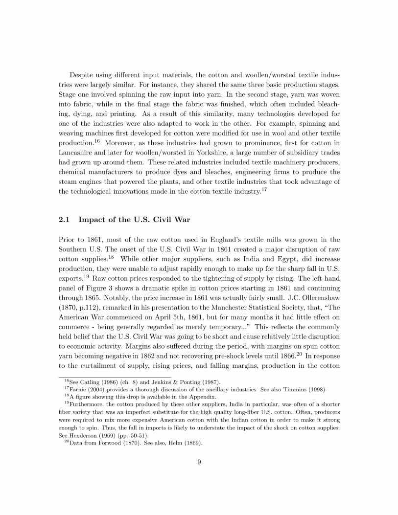
Prior to 1861, most of the raw cotton used in England’s textile mills was grown in theSouthern U.S. The onset of the U.S. Civil War in 1861 created a major disruption of rawcotton supplies.18 While other major suppliers, such as India and Egypt, did increaseproduction, they were unable to adjust rapidly enough to make up for the sharp fall in U.S.exports.19 Raw cotton prices responded to the tightening of supply by rising. The left-handpanel of Figure 3 shows a dramatic spike in cotton prices starting in 1861 and continuingthrough 1865. Notably, the price increase in 1861 was actually fairly small. J.C. Ollerenshaw(1870, p.112), remarked in his presentation to the Manchester Statistical Society, that, “TheAmerican War commenced on April 5th, 1861, but for many months it had little effect oncommerce - being generally regarded as merely temporary...” This reflects the commonlyheld belief that the U.S. Civil War was going to be short and cause relatively little disruptionto economic activity. Margins also suffered during the period, with margins on spun cottonyarn becoming negative in 1862 and not recovering pre-shock levels until 1866.20 In responseto the curtailment of supply, rising prices, and falling margins, production in the cotton
16See Catling (1986) (ch. 8) and Jenkins & Ponting (1987).17Farnie (2004) provides a thorough discussion of the ancillary industries. See also Timmins (1998).18A figure showing this drop is available in the Appendix.19Furthermore, the cotton produced by these other suppliers, India in particular, was often of a shorter
fiber variety that was an imperfect substitute for the high quality long-fiber U.S. cotton. Often, producers
were required to mix more expensive American cotton with the Indian cotton in order to make it strong
enough to spin. Thus, the fall in imports is likely to understate the impact of the shock on cotton supplies.
See Henderson (1969) (pp. 50-51).20Data from Forwood (1870). See also, Helm (1869).
9
textile industry fell. One of the best indicators of output in the industry is raw cottonconsumption, described in the right-hand panel of Figure 3. To summarize, the onset ofthe U.S. Civil War reduced cotton imports, increased prices, and decreased output. Theeffects started in 1861, peaked in 1862-3, and persisted through 1865.21 Figure 3 also showsthat by the late 1860s, the cotton textile industry had returned to its original growth path.Its expansion then continued with only relatively minor interruptions until WWI.22 Therecovery of production in the cotton textile industry is an important feature of the story,because it suggests that any long-term effect that the shock had on related industries had itsroots in the shock period, rather than in persistent changes to the cotton textile industry.23
To argue that the U.S. Civil War created a shock that was primarily industry-specific, welook for evidence of other large direct effects of the war. We would expect any such effectsto occur either through import or export channels. However, British import data fromMitchell (1988) suggest that, once raw material for textiles are removed, British importsshow no noticeable effect from the U.S. Civil War. Similarly, once textile exports areexcluded, British exports also show no negative effects.24 We may be particularly concernedthat the areas we study were directly affected by the U.S. Civil War through armamentindustries. However, none of the three armaments categories included in our data, “Guns”,“Ordinance”, and “Ships”, make up more than 0.2% of employment in any of towns includedin this study, during the study period, with the exception Liverpool, which is not includedin the anlysis for this reason.25
21Ollerenshaw (1870) stated that,“...we may consider 1862-5 as the years during which the effect of the
American war were really experienced,” adding later that,“The year 1866 is to be regarded as an exceptional
year [for cotton manufacturers], equally with 1861. The war was over but prices had fallen only 1d to 1.5d
per lb.”22Lazonick (1990) p. 138.23It is worth noting that the impact of the cotton shortage on manufacturers and traders in cotton textiles
was more complex than it appears from the foregoing graphs. A number of manufacturers and traders made
enormous profits at the beginning of the shock period, by selling stocks of cotton goods or raw cotton at
much higher prices. However, later in the shock period manufacturers often found their resources severely
strained (See Henderson (1969) (pp. 19-20)). For the rest of England, the early 1860s was generally a period
of prosperity, though there were financial crises in 1864 and 1866 as a result of a decline in English gold
reserves. This loss of reserves was due in part to a switch from purchasing raw cotton from American in
exchange for manufactured goods to purchasing from India, Egypt, or Brazil, where goods were generally
purchased with gold or silver. Importantly though, these financial crises affected England as a whole, and
should therefore not generated differential impacts between Lancashire and Yorkshire, except to the extent
that Lancashire banks and firms were more vulnerable due to the effects of the shock. The late 1860s, on the
other hand, was a period of poor economic performance throughout England, with numerous bankruptcies
among financial, commercial, railway, and manufacturing firms, a hangover from the earlier financial crises.24Graphs of British import and export data are available in the Appendix.25Shipbuilding made up roughly 2-4% of employment in Liverpool during the study period, and Liverpool
was active in providing ships used in the Civil War.
10
Figure 3: British Cotton Imports and Raw Cotton Prices 1815-1910
Raw Cotton Price on the Liverpool Market Raw Cotton Consumption 1815-1910
Data from Mitchell & Deane (1962).
Unlike cotton, the woollen and worsted industries show little effect from the shock.26 Itis not surprising that imports of raw wool are unaffected, since most of these imports comefrom Spain, Australia, South Africa, or South America. While there was some effect onwool textile exports to the U.S., this was made up for by an increase in exports to Europeanmarkets during the period, particularly to France following a new trade agreement in 1860,and through increased demand for military woolens.27
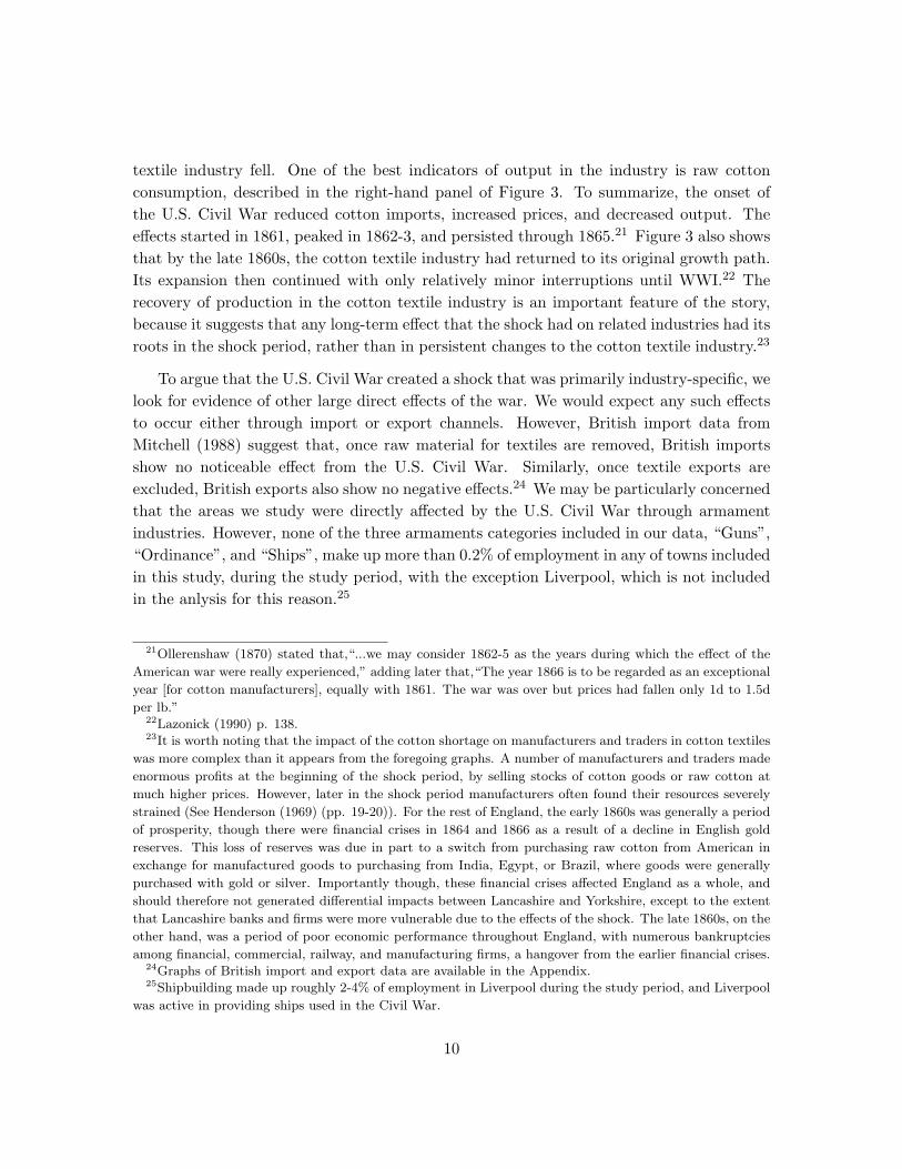
Given that we observe a strong negative shock to the cotton textile industry but littledirect effect on the woollen and worsted industries, we should expect the direct effects to bemuch stronger in Lancashire than in Yorkshire. This is confirmed by Figure 4, which showsthe number of able-bodied workers seeking relief from local Poor Law Boards as a fractionof the total 1861 population, in Lancashire and Yorkshire, over the shock period.28 ThesePoor Law Boards were the main apparatus through which relief was provided to paupersand the unemployed in England during this period.29
26Data from Mitchell & Deane (1962). Graphs are available in the Appendix.27Helm (1869) states, “in some of our foreign markets, linen and woolen goods have, as at home, taken
the place of cotton.” See also Jenkins & Ponting (1987) (p. 157-163) for a broad discussion of the effect of
the U.S. Civil War on wool and worsted textiles. While the U.S. imposed an additional tariff on wool textile
imports under The Morrill Tariff Act of 1861, wool textile exports to the United States rose steadily during
the 1860’s (Jenkins & Ponting (1987) p. 157-163) due to weak competition from domestic suppliers and the
need for heavy woolen goods for military uniforms and supplies.28Data are drawn from several of the major districts within each county, but do not cover the entire county.29Southall (1991) shows that Lancashire had the highest rate of pauperage of any English county in 1863,
with 10.3 percent of the population receiving Poor Law Relief, while the West Riding was among the lowest.
11
To summarize, while the U.S. Civil War generated an enormous negative shock to cottontextiles, a shock that fell heavily on Lancashire, it appears that other direct effects on theBritish economy were of limited size. In contrast to the experience of Lancashire, Yorkshire’smainstay wool textile industry shows little effect from the shock, and may have actuallybenefited somewhat from substitution away from higher priced cotton textiles. It is thislarge differential impact that is exploited in this study in order to pinpoint the effects ofthe shock on those industries that were related to cotton textiles.
Figure 4: Able-bodied relief seekers as a share of 1861 population
Data from Southall et al. (1998).
3 Data
The primary database used in this study is drawn from the the British Census of Population.These decennial Censuses are the best available source of information on the structure ofthe British economy over the period of this study, 1851-1891.30 For each census, occupationdata was collected from respondents by trained registrars, and each census report presentssummaries of employment by occupational category.31 The number of occupational cate-gories in these reports varies somewhat over the period studied, with a high of 478 categoriesin 1861 and a low of 348 in 1891.
A similar pattern holds when Southall looks only at able-bodied relief seekers. In contrast, in other cyclical
downturns occurring during the study period, such as those 1868 and 1879, Southall finds that relief rates
in Lancashire and Yorkshire were similar.30See Lee (1979) p. 3.31Woolard (1999) compares these summary tables to the original enumerators books from the Isle of Man
in 1881 and finds that “the original process of classification was remarkably accurate in light of the rules
applied” (p. 29), particularly in the manufacturing and industrial categories.
12
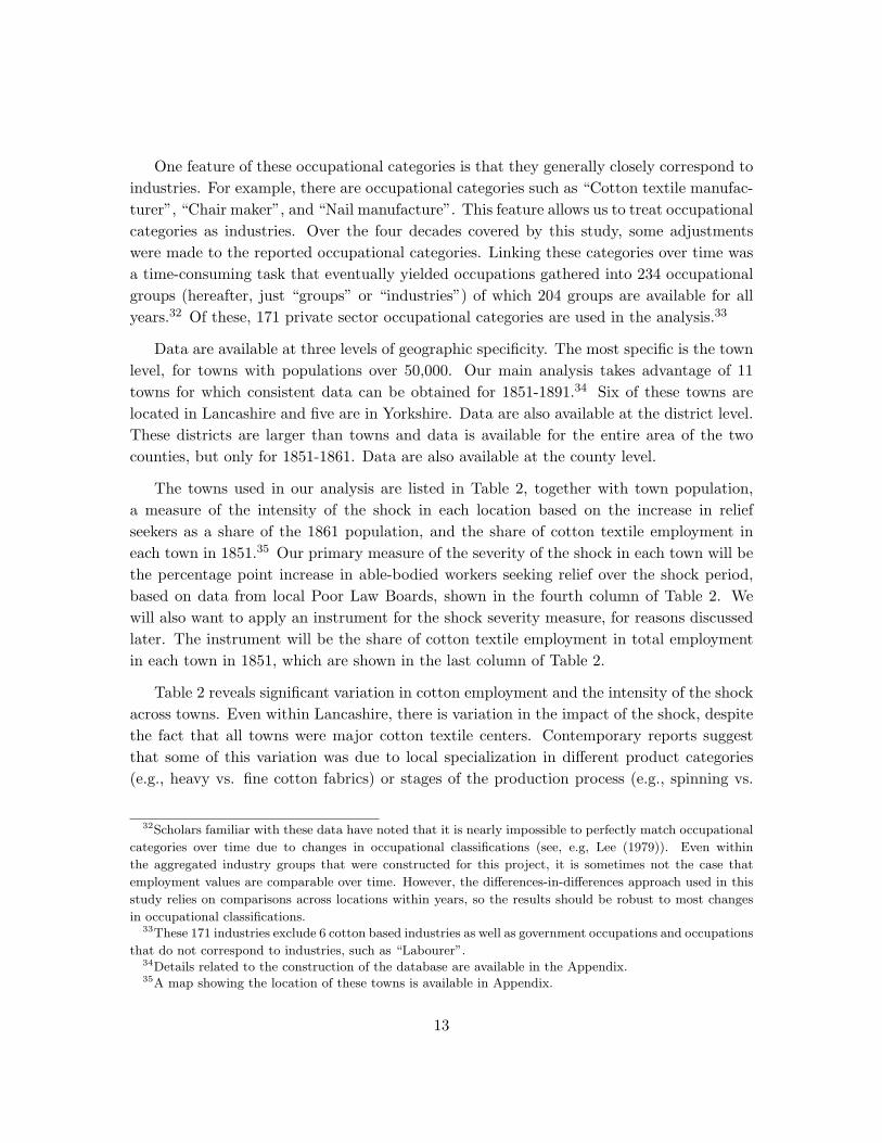
One feature of these occupational categories is that they generally closely correspond toindustries. For example, there are occupational categories such as “Cotton textile manufac-turer”, “Chair maker”, and “Nail manufacture”. This feature allows us to treat occupationalcategories as industries. Over the four decades covered by this study, some adjustmentswere made to the reported occupational categories. Linking these categories over time wasa time-consuming task that eventually yielded occupations gathered into 234 occupationalgroups (hereafter, just “groups” or “industries”) of which 204 groups are available for allyears.32 Of these, 171 private sector occupational categories are used in the analysis.33
Data are available at three levels of geographic specificity. The most specific is the townlevel, for towns with populations over 50,000. Our main analysis takes advantage of 11towns for which consistent data can be obtained for 1851-1891.34 Six of these towns arelocated in Lancashire and five are in Yorkshire. Data are also available at the district level.These districts are larger than towns and data is available for the entire area of the twocounties, but only for 1851-1861. Data are also available at the county level.
The towns used in our analysis are listed in Table 2, together with town population,a measure of the intensity of the shock in each location based on the increase in reliefseekers as a share of the 1861 population, and the share of cotton textile employment ineach town in 1851.35 Our primary measure of the severity of the shock in each town will bethe percentage point increase in able-bodied workers seeking relief over the shock period,based on data from local Poor Law Boards, shown in the fourth column of Table 2. Wewill also want to apply an instrument for the shock severity measure, for reasons discussedlater. The instrument will be the share of cotton textile employment in total employmentin each town in 1851, which are shown in the last column of Table 2.
Table 2 reveals significant variation in cotton employment and the intensity of the shockacross towns. Even within Lancashire, there is variation in the impact of the shock, despitethe fact that all towns were major cotton textile centers. Contemporary reports suggestthat some of this variation was due to local specialization in different product categories(e.g., heavy vs. fine cotton fabrics) or stages of the production process (e.g., spinning vs.
32Scholars familiar with these data have noted that it is nearly impossible to perfectly match occupational
categories over time due to changes in occupational classifications (see, e.g, Lee (1979)). Even within
the aggregated industry groups that were constructed for this project, it is sometimes not the case that
employment values are comparable over time. However, the differences-in-differences approach used in this
study relies on comparisons across locations within years, so the results should be robust to most changes
in occupational classifications.33These 171 industries exclude 6 cotton based industries as well as government occupations and occupations
that do not correspond to industries, such as “Labourer”.34Details related to the construction of the database are available in the Appendix.35A map showing the location of these towns is available in Appendix.
13
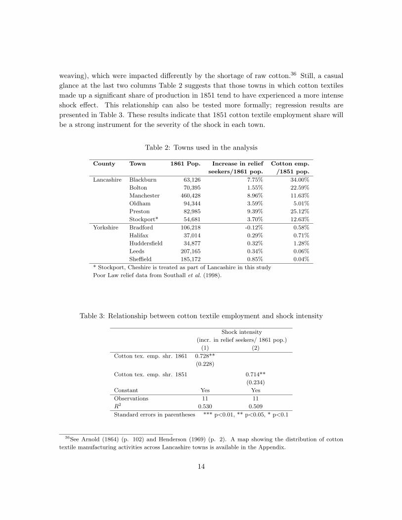
weaving), which were impacted differently by the shortage of raw cotton.36 Still, a casualglance at the last two columns Table 2 suggests that those towns in which cotton textilesmade up a significant share of production in 1851 tend to have experienced a more intenseshock effect. This relationship can also be tested more formally; regression results arepresented in Table 3. These results indicate that 1851 cotton textile employment share willbe a strong instrument for the severity of the shock in each town.
Table 2: Towns used in the analysis
County Town 1861 Pop. Increase in relief Cotton emp.
seekers/1861 pop. /1851 pop.
Lancashire Blackburn 63,126 7.75% 34.00%
Bolton 70,395 1.55% 22.59%
Manchester 460,428 8.96% 11.63%
Oldham 94,344 3.59% 5.01%
Preston 82,985 9.39% 25.12%
Stockport* 54,681 3.70% 12.63%
Yorkshire Bradford 106,218 -0.12% 0.58%
Halifax 37,014 0.29% 0.71%
Huddersfield 34,877 0.32% 1.28%
Leeds 207,165 0.34% 0.06%
Sheffield 185,172 0.85% 0.04%
* Stockport, Cheshire is treated as part of Lancashire in this study
Poor Law relief data from Southall et al. (1998).
Table 3: Relationship between cotton textile employment and shock intensity
Shock intensity
(incr. in relief seekers/ 1861 pop.)
(1) (2)
Cotton tex. emp. shr. 1861 0.728**
(0.228)
Cotton tex. emp. shr. 1851 0.714**
(0.234)
Constant Yes Yes
Observations 11 11
R2 0.530 0.509
Standard errors in parentheses *** p<0.01, ** p<0.05, * p<0.1
36See Arnold (1864) (p. 102) and Henderson (1969) (p. 2). A map showing the distribution of cotton
textile manufacturing activities across Lancashire towns is available in the Appendix.
14
While the data set spans 171 industries and 11 towns, not all industries have positiveemployment in all towns in all years. Because we work with log employment, location-industries with no employment will result in missing entries. For the analysis, we willinclude only location-industries that have positive employment levels for all five years. Theresult will be an unbalanced panel with 1,543 complete location-industries. In essence,this analysis will be on the intensive margin of employment, i.e., changes in employmentlevels in industries present in a location, while ignoring the extensive margin, i.e., industriesemerging or disappearing in a location. This makes sense given that our focus is on therole of inter-industry spillovers, which presumably exist primarily when both industries arepresent in a location.
3.1 Industry relatedness
One important input into the analysis is a measure of relatedness between the cotton textileindustry and other industries in the economy. Two approaches are taken to measuring thepattern of relatedness. The first uses the British Census data to construct a relatednessmeasure based on the geographic coagglomeration of industries. This measure is inspiredby Ellison & Glaeser (1997), as well as, Ellison et al. (2010), who find that geographic coag-glomeration patterns are correlated with measures of technological spillovers, occupationalsimilarity, and input-output flows.37 Thus, the advantage of this measure is that it mayreflect many forms of relatedness, though this comes at the cost of not being able to identifythe particular types of industry connections that matter the most. Geographic coagglomer-ation is measured for each pair of industries and reflects the propensity of the two industriesto concentrate production in the same location, where concentration implies that the sizeof the industry is in excess of the size that would be predicted given the location’s overallsize (population). Specifics of the calculation of the coagglomeration measure are availablein the Appendix.
It is important to note that the geographic coagglomeration measure is calculated usingthe district level census data, which are different from the town-level data used as theprimary outcome variable. The district-level data are significantly more geographicallycomprehensive than the town-level data, giving us more regions to work with (71 districtsvs. 11 towns). Furthermore, we can calculated an alternative coagglomeration droppingall of the districts containing towns available in the town-level data and show that thisalternative coagglomeration measure delivers similar results.
37One critique of this approach is Helsley & Strange (2010), who show that coagglomeration patterns across
locations may be inefficient. This should, if anything, cause Ellison et al. (2010) to understate the strength
of the relationship between their measures of inter-industry connections and coagglomeration patterns.
15
One way to check the reasonableness of the geographic coagglomeration relatednessmeasure is to consider the least and most related industries.38 At the top of the related listis cotton textile production, followed by cotton textile finishing. Other textile industries,such as woollen, worsted, thread, and miscellaneous weaving, are also among the top 15 mostrelated. This may reflect technological spillovers, labor market pooling, or other forms ofinter-industry connections. The third most related industry is paper manufacturing, whichmay seem odd at first, but an important input for this industry at the time was waste cotton.The sixth most related industry, coal mining, produced the second most important materialinput for the cotton textile industry. Engine and machine makers, an industry discussedin more detail in Section 4, ranks thirteenth. Toll collector and road construction alsorank among the top 15, reflecting the importance of road transport in the cotton districts.Among the fifteen least coagglomerated industries, there are none that one would naturallyexpect to be related to cotton textiles. Examples include ship transport, sugar refining,cooper, lodging-house keeper, and tobacconist. Overall, it appears that coagglomeration isproviding us with a reasonable measure of relatedness between industries.
A coagglomeration measure of relatedness to the wool textile industry, calculated usingdata from Yorkshire, gives relatedness patterns that are fairly similar to that observed forcotton in Lancashire. The correlation between these two coagglomeration measures is 0.3.39
The second measure of relatedness is based on an input-output matrix for intermediategoods. This matrix is based on one constructed by Thomas (1987), and divides the economyinto 42 industries.40 The primary source used by Thomas to construct his input-outputmatrix was the 1907 Census of Production, Britain’s first industrial census, though he alsodrew on a wealth of supplementary information. Because this input-output matrix wasconstructed using data from after the study period, there is some worry that input-outputrelationships may have changed between the beginning of the study period and the 1907Census of Production. One way to test for such changes is to compare this input-outputmatrix to a less detailed matrix constructed by Horrell et al. (1994) for 1841, which dividesthe economy into 17 categories. Once the categories in these matrices are matched, we findthat the correlation between their entries is high (> .96), giving us confidence that ourinput-output matrix is relevant for the period covered by this study.
38A table showing the most and least coagglomerated industries is available in the Appendix.39This figure exclude cotton, woollen, and worsted textile manufacturing.40Details of the adjustments made to the original Thomas (1987) input-output matrix are available in the
Appendix.
16
4 An Example: Engine & Machine Makers
This section explores the impact of the shock on one related industry, “Engine & MachineMakers” (E&M).41 There are two reasons to give the E&M industry special attention. First,a number of scholars have argued that this industry played a central role in the industrialrevolution, and in Britain’s economic success throughout the 19th century.42 Second, thisindustry appears to be closely related to the cotton textile industry in Lancashire, andalso to the woollen and worsted industries in Yorkshire. Farnie (2004) writes that “Textileengineering became the most important of all the ancillary trades [to cotton textiles]. Itslight engineering section supplied spinning machines and looms and a whole succession ofrelated equipment, while its heavy engineering industry supplied steam engines, boilers,and mechanical stokers.” The coagglomeration relatedness measure indicates a high level ofrelatedness between textile manufacturing and E&M. According to this measure, E&M isthe 9th most related industry to cotton textiles in Lancashire (out of the 171 included in theanalysis dataset), and the 26th most related to wool textiles in Yorkshire. The intermediategoods input-output matrix does not show significant flows between these industries, sincethe E&M industry primarily produced capital goods.
Connections between the E&M and cotton textile producers likely took multiple forms.The most obvious connection was direct backward demand linkages from textile producersto the firms supplying their machinery, at least for a subset of E&M firms. Two-way knowl-edge and technology flows between these industries may have also been important, thoughevidence of such flows is necessarily sparse. One indication of their importance is the factthat machinery firms often specialized in machinery catered to the needs of producers intheir local area. For example, Bolton machine makers dominated the market for machineryto spin fine thread counts, which was mainly produced in the Bolton area.43, while Oldhamproducers were dominant in the machinery for spinning of heavier thread counts, whereOldham producers dominated production. Given the relatively close proximity of these lo-cations, there seem to be few reasons, other than knowledge flows between textile and E&Mproducers, that explain this specialization pattern. Furthermore, it is well documented thatoperators in the textile mills were active in “tweaking” their machines, to the point where,for example, “no two pairs of [spinning] mules worked in precisely the same way”.44 It
41Other highly related industries display similar patterns to those described for the E&M industry in this
section, including “Worsted Manufacturing”, “Stone Workers”, “Brick Making”, “Dying and Calendering”,
“Millwrights”, “Iron Manufacture”, “Hoisery”, “Silk”, and “Flax and Linen”.42For example, Allen (2009) argues that “the great achievement of the British Industrial Revolution was,
in fact, the creation of the first large engineering industry that could mass-produce productivity-raising
machinery.”43See Catling (1986) (ch. 7).44Lazonick (1990) (p. 96).
17
seems reasonable to expect that productivity advances made through such tweaking wouldeventually be incorporated by local machine producers. The textile and engineering indus-tries may have also been linked through labor market connections. Marshall (1920) (p. 226)suggests that textile firms located near E&M firms (or vice-versa) because these industriesused complementary sets of labor.45 Given these connections, we may expect the shock toreduce the growth rate of the E&M industry in locations that were more severely impactedby the cotton shortage.
The pattern of growth of the E&M industry across towns over the study period isexplored in Figure 5. The left-hand panel of this figure presents the sum of log employmentfor towns in Lancashire (high shock intensity) compared to the sum over towns in Yorkshire(low shock intensity).46 The right-hand panel presents the sum of log employment in towns,where the towns have been grouped based on the share of their employment in cotton textilesin 1851, our instrument for the intensity of the shock.47 These figures suggest that the shockled to a slowdown in the growth of the E&M industries in locations in which cotton textileswere initially more important, which tended to be the locations that were more severelyimpacted by the shock. While the increase in log employment was similar in towns with highand low cotton textile employment shares prior to 1861, there was divergence in 1871-1891,with the towns in which cotton textiles were less important gaining a relative advantage inthe E&M industry.
Given the available data, it is not possible to pinpoint which types of inter-industryconnections are driving the observed effects. However, given that we observe effects whichpersist several decades after the end of the cotton shortage and the recovery of the cottontextile industry, it is clear that these effects cannot be driven by contemporaneous demandlinkages alone. Rather, the appearance of the persistent divergence following the shocksuggests that the temporary recession in cotton textile production was transmitted throughinter-industry connections and generated long-lasting impacts on the relative productivity
45Textile production employed many women and children, while E&M firms employed almost exclusively
adult males. Marshall (1920) argued that by co-locating, these firms could pay lower wages and still achieve
similar total household incomes levels. Note that this is the opposite of how most economists think of the
labor market pooling effect today, which involves benefits to firms employing similar labor forces through
co-locating. Marshall acknowledged both of these potential benefits, but less attention has been paid to the
benefits of co-location for industries employing different labor forces.46Graphs showing the sum of log employment are shown rather than those showing the log of the sum of
employment across towns because the former reduces the influence of outlier towns in the graph and also
because this corresponds more directly to the econometric methodology. The main outlier is Oldham which
was the home of the most dominant engineering firm over the period, Platt Bros. of Oldham, which does
not appear to have suffered as much from the shock, perhaps due to the benefits of economies of scale or
market power.47The groups are: high – Blackburn, Bolton, and Preston; medium – Manchester, Oldham, and Stockport;
low – Bradford, Halifax, Huddersfield, Leeds, Sheffield.
18
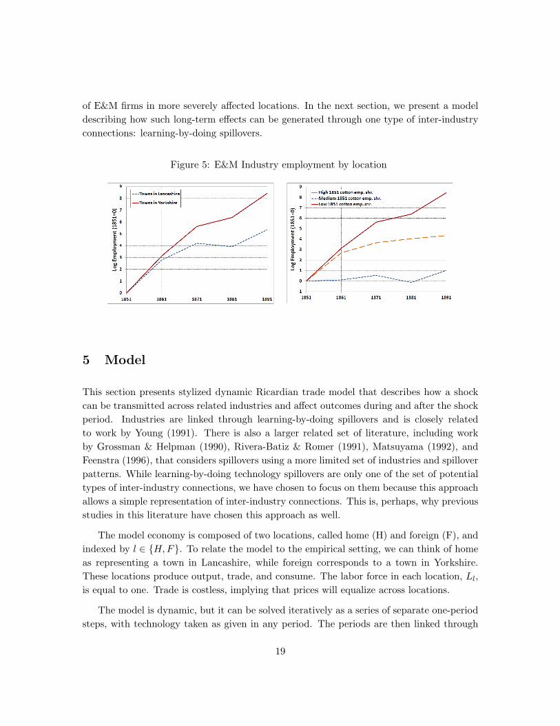
of E&M firms in more severely affected locations. In the next section, we present a modeldescribing how such long-term effects can be generated through one type of inter-industryconnections: learning-by-doing spillovers.
Figure 5: E&M Industry employment by location
5 Model
This section presents stylized dynamic Ricardian trade model that describes how a shockcan be transmitted across related industries and affect outcomes during and after the shockperiod. Industries are linked through learning-by-doing spillovers and is closely relatedto work by Young (1991). There is also a larger related set of literature, including workby Grossman & Helpman (1990), Rivera-Batiz & Romer (1991), Matsuyama (1992), andFeenstra (1996), that considers spillovers using a more limited set of industries and spilloverpatterns. While learning-by-doing technology spillovers are only one of the set of potentialtypes of inter-industry connections, we have chosen to focus on them because this approachallows a simple representation of inter-industry connections. This is, perhaps, why previousstudies in this literature have chosen this approach as well.
The model economy is composed of two locations, called home (H) and foreign (F), andindexed by l ∈ {H,F}. To relate the model to the empirical setting, we can think of homeas representing a town in Lancashire, while foreign corresponds to a town in Yorkshire.These locations produce output, trade, and consume. The labor force in each location, Ll,is equal to one. Trade is costless, implying that prices will equalize across locations.
The model is dynamic, but it can be solved iteratively as a series of separate one-periodsteps, with technology taken as given in any period. The periods are then linked through
19
technological spillovers, which, being external to firms, do not affect the equilibrium in aparticular period. Therefore, we solve a one-period version of the model first and thendescribe how outcomes from one period determine technology levels in the next. Timesubscripts are suppressed until the dynamic elements of the model are introduced.
There are two sectors in the economy, a differentiated good sector, and a homogeneousgood sector. The homogeneous good is numeraire, so pG = 1. Individuals’ utility overthese sectors is given below, where D is an index of differentiated good consumption, G isconsumption of the homogeneous good, and µ ∈ (0, 1).
U = DµG1−µ
Within the differentiated goods sector, there are a fixed number N goods, indexed byi ∈ {1, ..., N}, which also correspond to industries. Individuals’ utility is such that the indexof differentiated goods consumption takes a Cobb-Douglas form, where di is the quality ofconsumption of good i, γi ∈ (0, 1), and
∑Ni=1 γi = 1.
D =N∏i=1
dγii
Within each industry, home and foreign each produce one variety, so there are 2Ntotal varieties of differentiated goods. Preferences over these varieties take a CES form,where xil is consumption of the variety of good i produced in location l, and ρ ∈ (0, 1). Thecorresponding price index for each differentiated good sector is given by pi, where qil denotesthe price of the variety of good i produced in location l, and σ = 1/(1− ρ) ∈ (1,+∞).
di = (xρiH + xρiF )1ρ pi =
(q1−σiH + q1−σiF
) 11−σ
Thus, the economy has three levels of product specificity: the sector level, the goodslevel, and the variety level. This utility setup may seem over-complicated at first glance, yetit provides some advantages that will help simplify our analysis. First, this framework willallow firms in both locations to produce positive quantities and compete in each industry(though with different varieties), even with perfect competition between firms. Second,the Cobb-Douglas formulation means that shocks to one industry will not impact otherindustries through general price index effects. This is an important simplification that willallow us to focus only on inter-industry impacts through technology spillovers. Letting Erepresent total expenditures in the economy, it can be shown that expenditures in each
20
differentiated goods industries (Ei), and for the homogeneous good (EG), respectively, areEi = µγiE and EG = (1− µ)E.
Next, consider the production side of the economy. The homogeneous good sector iscomposed of many perfectly competitive firms that produce output using labor only, withthe production function G = LG. If a location produces the homogeneous good, then thewage in that location is wl = pG = 1. Production in a differentiated goods industry i inlocation l depends on technology Ail and labor Lil. Within each differentiated good industryand location there are many perfectly competitive firms, denoted with the subscript f. Thus,the production function is xilf = AilLilf . Firms can freely copy new technologies from oneanother, so all firms in the same industry and location share the same technology level.However, this information does not flow across locations, so technology in home may differfrom that in foreign in the same industry.48 Given these production functions, perfectcompetition implies the following price levels for each differentiated good variety.
qil =wlAil
(1)
The differentiated goods production function, price, and demand equations, can be usedto derive output and employment for each industry and variety in the differentiated goodssector, even though output for any particular firm in an industry is indeterminate.
xil = Eipσ−1i q−σil (2)
Lil = Eipσ−1i q−σil A
−1il (3)
Using the price levels for a variety from Equation 1, it is possible to express the priceindex for each good, and for all goods, in terms of wages, technology, and exogenous pa-rameters only. This in turn allows us to express output and employment in terms of onlywages, technology, and exogenous parameters, using Equations 2 and 3.
5.1 Solving within a period
Solving for outcomes within a particular period, taking technology as given, involves assum-ing perfect competition and labor market clearing. The assumption of perfect competition
48This is consistent with results indicating that spillovers are sharply attenuated with distance. See, e.g.,
Rosenthal & Strange (2001), Bottazzi & Peri (2003), and Arzaghi & Henderson (2008). Feenstra (1996)
shows the importance of this assumption and provides a review of some related empirical literature.
21
has already been used to derive the price equations above. Labor market clearing requiresthat the sum of all of the individual labor demands for a location equal the total laborforce in that location, i.e., such that L = LGl +
∑Ni=1 Lil. Given Equations 1 and 3, we
can write employment in the differentiated goods industry as a function of only wages andexpenditures. Expenditures can also be written as a function of wages since, with all incomebeing spent in any given period, it must be the case that E = L(wH + wF ). Thus, findingthe equilibrium in a particular period amounts to finding the wages that clear the labormarket.
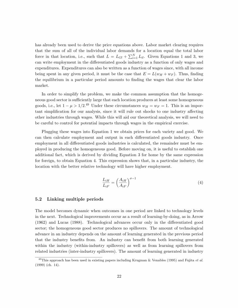
In order to simplify the problem, we make the common assumption that the homoge-neous good sector is sufficiently large that each location produces at least some homogeneousgoods, i.e., let 1− µ > 1/2.49 Under these circumstances wH = wF = 1. This is an impor-tant simplification for our analysis, since it will rule out shocks to one industry affectingother industries through wages. While this will aid our theoretical analysis, we will need tobe careful to control for potential impacts through wages in the empirical exercise.
Plugging these wages into Equation 1 we obtain prices for each variety and good. Wecan then calculate employment and output in each differentiated goods industry. Onceemployment in all differentiated goods industries is calculated, the remainder must be em-ployed in producing the homogeneous good. Before moving on, it is useful to establish oneadditional fact, which is derived by dividing Equation 3 for home by the same expressionfor foreign, to obtain Equation 4. This expression shows that, in a particular industry, thelocation with the better relative technology will have higher employment.
LiHLiF
=(AiHAiF
)σ−1
(4)
5.2 Linking multiple periods
The model becomes dynamic when outcomes in one period are linked to technology levelsin the next. Technological improvements occur as a result of learning-by-doing, as in Arrow(1962) and Lucas (1988). Technological advances occur only in the differentiated goodsector; the homogeneous good sector produces no spillovers. The amount of technologicaladvance in an industry depends on the amount of learning generated in the previous periodthat the industry benefits from. An industry can benefit from both learning generatedwithin the industry (within-industry spillovers) as well as from learning spillovers fromrelated industries (inter-industry spillovers). The amount of learning generated in industry
49This approach has been used in existing papers including Krugman & Venables (1995) and Fujita et al.
(1999) (ch. 14).
22

j that industry i benefits from depends on the parameter τ ij , as shown in Equation 5.Thus, there is an n x n matrix of τ ij parameters that represent the extent to which learninggenerated by employment in industry j benefits industry i. The only restriction on theseparameters is that τ ij ≥ 0 for all i and j.50 Note that in this expression spillovers dependon Ljlt + 1 rather than simply Ljlt. This ensures that spillovers from industry j will be zerowhen Ljlt = 0 and positive whenever Ljlt > 0 and τ ij > 0.
ln(Ailt+1)− ln(Ailt) = Silt =N∑j=1
τ ijln(Ljlt + 1) (5)
This expression gives the technology level in any period, given outcomes in the previousperiod. Thus, given a set of initial technology levels, the model can now be solved for allfuture periods.
5.3 A cost shock
The economic shock is introduced into the model as an additional cost φ > 0 that must bepaid for production in one differentiated good industry, denoted i = C (for Cotton) for oneperiod, hereafter labeled period s.51 The price for the variety of good C from location l inperiod s is as follows.
qCls =wlsACls
+ φ (6)
Observation 1 describes the effects of the shock in the shock period, where we presumethat industry C has better technology in home than in foreign at the beginning of the shockperiod.
50It may be surprising at first that we do not assume that within-industry spillovers are larger than cross-
industry spillovers, but there are reasons to think that cross-industry spillovers may be larger. For example,
firms may have more incentive to hide knowledge from competitors in their industry but to collaborate with
firms in other industries. See Kugler (2006) for more on this topic.51This reduced-form approach can be motivated by a model that explicitly incorporates intermediate
goods in production, as shown in the Appendix.
23
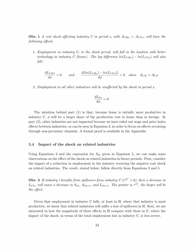
Obs. 1 A cost shock affecting industry C in period s, with ACHs > ACFs, will have thefollowing effects.
1. Employment in industry C, in the shock period, will fall in the location with bettertechnology in industry C (home). The log difference ln(LCHs) − ln(LCFs) will alsofall.
dLCHsdφ
< 0 andd(ln(LCHs)− ln(LCFs))
dφ< 0 when ACH > ACF
2. Employment in all other industries will be unaffected by the shock in period s,
dLilsdφ
= 0
The intuition behind part (1) is that, because home is initially more productive inindustry C, φ will be a larger share of the production cost in home than in foreign. Inpart (2), other industries are not impacted because we have ruled out wage and price indexeffects between industries, as can be seen in Equation 3, in order to focus on effects occurringthrough non-pecuniary channels. A formal proof is available in the Appendix.
5.4 Impact of the shock on related industries
Using Equations 3 and the expression for Silt given in Equation 5, we can make someobservations on the effect of the shock on related industries in future periods. First, considerthe impact of a reduction in employment in the industry receiving the negative cost shockon related industries. The result, stated below, follow directly from Equations 3 and 5.
Obs. 2 If industry i benefits from spillovers from industry C (τ iC > 0), then a decrease inLCls, will cause a decrease in Sils, Ails+1, and Lils+1. The greater is τ iC , the larger will bethe effect.
Given that employment in industry C falls, at least in H, where that industry is mostproductive, we know that related industries will suffer a loss of spillovers in H. Next, we areinterested in how the magnitude of these effects in H compare with those in F, where theimpact of the shock, in terms of the total employment lost in industry C, is less severe.
24
Obs. 3 The loss of spillovers in industries related to industry C in the shock period s willbe larger in the location in which industry C is initially more productive. I.e., for someindustry i with τ iC > 0,
dSiHsdφ
>dSiFsdφ
when ACHs > ACFs
The intuition here is that the loss of spillovers in related industries will be larger in thelocation in which the loss of employment in industry C is greater. A formal proof is availablein the Appendix. Naturally, the differential impact on the level of spillovers in period s willlead to differential impacts on the level of technology and employment in period s+1. Theresults above describe the impact of the shock on technology and employment in relatedindustries in period s+1. We can also speculate about the impacts in periods beyond s+1,though here the effects will become more complicated.
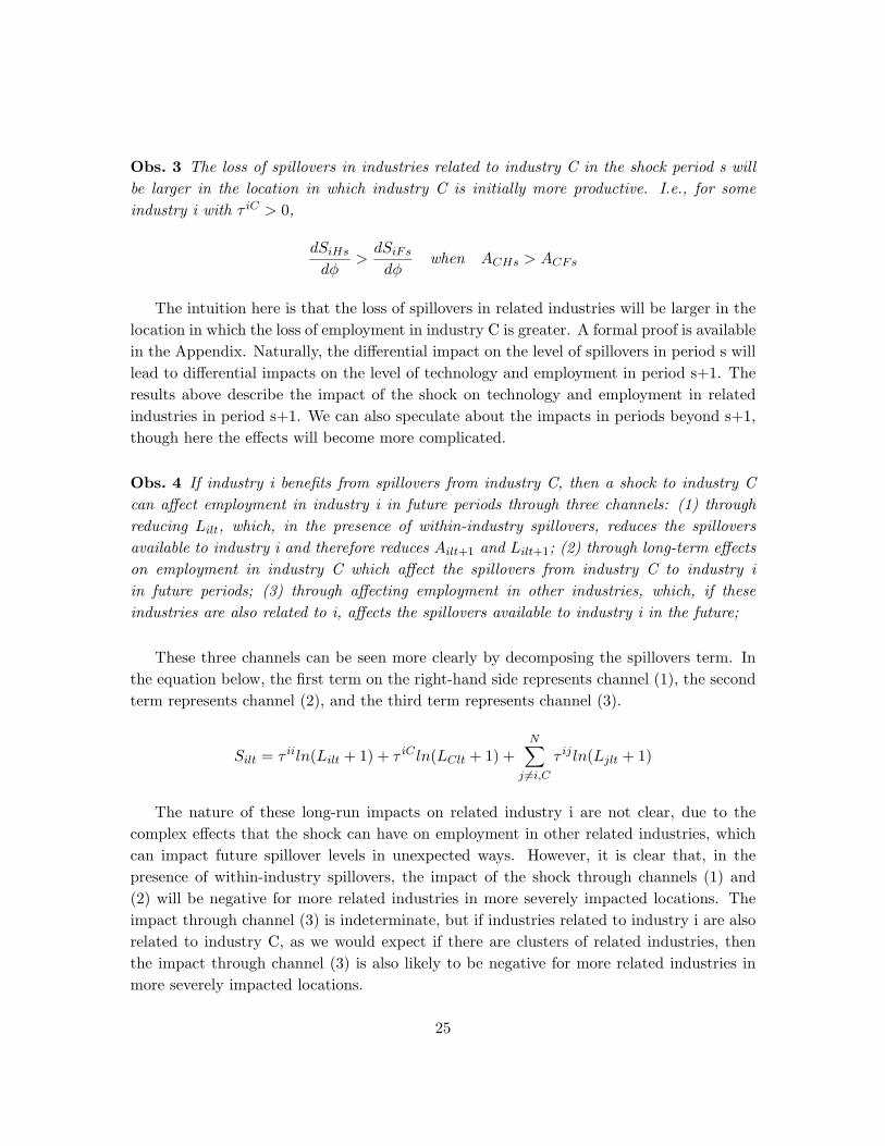
Obs. 4 If industry i benefits from spillovers from industry C, then a shock to industry Ccan affect employment in industry i in future periods through three channels: (1) throughreducing Lilt, which, in the presence of within-industry spillovers, reduces the spilloversavailable to industry i and therefore reduces Ailt+1 and Lilt+1; (2) through long-term effectson employment in industry C which affect the spillovers from industry C to industry iin future periods; (3) through affecting employment in other industries, which, if theseindustries are also related to i, affects the spillovers available to industry i in the future;
These three channels can be seen more clearly by decomposing the spillovers term. Inthe equation below, the first term on the right-hand side represents channel (1), the secondterm represents channel (2), and the third term represents channel (3).
Silt = τ iiln(Lilt + 1) + τ iC ln(LClt + 1) +N∑
j 6=i,Cτ ijln(Ljlt + 1)
The nature of these long-run impacts on related industry i are not clear, due to thecomplex effects that the shock can have on employment in other related industries, whichcan impact future spillover levels in unexpected ways. However, it is clear that, in thepresence of within-industry spillovers, the impact of the shock through channels (1) and(2) will be negative for more related industries in more severely impacted locations. Theimpact through channel (3) is indeterminate, but if industries related to industry i are alsorelated to industry C, as we would expect if there are clusters of related industries, thenthe impact through channel (3) is also likely to be negative for more related industries inmore severely impacted locations.
25
Of these three channels, channel (3) is the most elusive, but it may well be the mostimportant. Previous studies looking at the impacts of spillovers through input-output link-ages due to FDI, such as Aitken & Harrison (1999), have found little evidence of spilloversbetween firms within the same industry. On the other hand, studies such as Javorcik (2004),Kugler (2006), and Amiti & Cameron (2007) have found evidence of spillovers between firmsin different industries. Kugler (2006) argues that this makes sense, because firms are likelyto hide information from their competitors while cooperating with firms that they do notcompete with, such as their suppliers and customers.
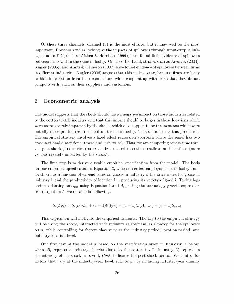
6 Econometric analysis
The model suggests that the shock should have a negative impact on those industries relatedto the cotton textile industry and that this impact should be larger in those locations whichwere more severely impacted by the shock, which also happen to be the locations which wereinitially more productive in the cotton textile industry. This section tests this prediction.The empirical strategy involves a fixed effect regression approach where the panel has twocross sectional dimensions (towns and industries). Thus, we are comparing across time (pre-vs. post-shock), industries (more vs. less related to cotton textiles), and locations (morevs. less severely impacted by the shock).
The first step is to derive a usable empirical specification from the model. The basisfor our empirical specification is Equation 3, which describes employment in industry i andlocation l as a function of expenditures on goods in industry i, the price index for goods inindustry i, and the productivity of location l in producing its variety of good i. Taking logsand substituting out qilt using Equation 1 and Ailt using the technology growth expressionfrom Equation 5, we obtain the following.
ln(Lilt) = ln(µγiE) + (σ − 1)ln(pit) + (σ − 1)ln(Ailt−1) + (σ − 1)Silt−1
This expression will motivate the empirical exercises. The key to the empirical strategywill be using the shock, interacted with industry relatedness, as a proxy for the spilloversterm, while controlling for factors that vary at the industry-period, location-period, andindustry-location level.
Our first test of the model is based on the specification given in Equation 7 below,where Ri represents industry i’s relatedness to the cotton textile industry, Vl representsthe intensity of the shock in town l, Postt indicates the post-shock period. We control forfactors that vary at the industry-year level, such as pit by including industry-year dummy
26
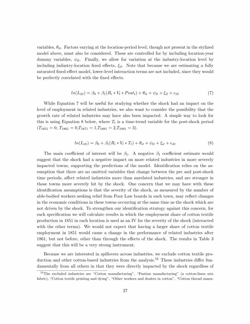
variables, θit. Factors varying at the location-period level, though not present in the stylizedmodel above, must also be considered. These are controlled for by including location-yeardummy variables, ψlt. Finally, we allow for variation at the industry-location level byincluding industry-location fixed effects, ξil. Note that because we are estimating a fullysaturated fixed-effect model, lower-level interaction terms are not included, since they wouldbe perfectly correlated with the fixed effects.
ln(Lilt) = β0 + β1(Ri ∗ Vl ∗ Postt) + θit + ψlt + ξil + εilt (7)
While Equation 7 will be useful for studying whether the shock had an impact on thelevel of employment in related industries, we also want to consider the possibility that thegrowth rate of related industries may have also been impacted. A simple way to look forthis is using Equation 8 below, where Tt is a time-trend variable for the post-shock period(T1851 = 0, T1861 = 0,T1871 = 1,T1881 = 2,T1891 = 3).
ln(Lilt) = β0 + β1(Ri ∗ Vl ∗ Tt) + θit + ψlt + ξil + εilt (8)
The main coefficient of interest will be β1. A negative β1 coefficient estimate wouldsuggest that the shock had a negative impact on more related industries in more severelyimpacted towns, supporting the predictions of the model. Identification relies on the as-sumption that there are no omitted variables that change between the pre and post-shocktime periods, affect related industries more than unrelated industries, and are stronger inthose towns more severely hit by the shock. One concern that we may have with theseidentification assumptions is that the severity of the shock, as measured by the number ofable-bodied workers seeking relief from Poor Law boards in each town, may reflect changesin the economic conditions in these towns occurring at the same time as the shock which arenot driven by the shock. To strengthen our identification strategy against this concern, foreach specification we will calculate results in which the employment share of cotton textileproduction in 1851 in each location is used as an IV for the severity of the shock (interactedwith the other terms). We would not expect that having a larger share of cotton textileemployment in 1851 would cause a change in the performance of related industries after1861, but not before, other than through the effects of the shock. The results in Table 3suggest that this will be a very strong instrument.
Because we are interested in spillovers across industries, we exclude cotton textile pro-duction and other cotton-based industries from the analysis.52 These industries differ fun-damentally from all others in that they were directly impacted by the shock regardless of
52The excluded industries are “Cotton manufacturing”, “Fustian manufacturing” (a cotton-linen mix
fabric), “Cotton textile printing and dying”, “Other workers and dealers in cotton”, “Cotton thread manu-
27
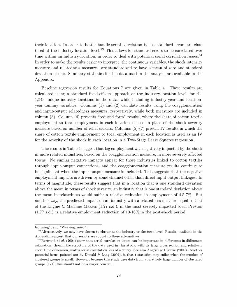
their location. In order to better handle serial correlation issues, standard errors are clus-tered at the industry-location level.53 This allows for standard errors to be correlated overtime within an industry-location, in order to deal with potential serial correlation issues.54
In order to make the results easier to interpret, the continuous variables, the shock intensitymeasure and relatedness measures, are standardized to have a mean of zero and standarddeviation of one. Summary statistics for the data used in the analysis are available in theAppendix.
Baseline regression results for Equations 7 are given in Table 4. These results arecalculated using a standard fixed-effects approach at the industry-location level, for the1,543 unique industry-locations in the data, while including industry-year and location-year dummy variables. Columns (1) and (2) calculate results using the coagglomerationand input-output relatedness measures, respectively, while both measures are included incolumn (3). Column (4) presents “reduced form” results, where the share of cotton textileemployment to total employment in each location is used in place of the shock severitymeasure based on number of relief seekers. Columns (5)-(7) present IV results in which theshare of cotton textile employment to total employment in each location is used as an IVfor the severity of the shock in each location in a Two-Stage Least Squares regression.
The results in Table 4 suggest that log employment was negatively impacted by the shockin more related industries, based on the coagglomeration measure, in more severely affectedtowns. No similar negative impacts appear for those industries linked to cotton textilesthrough input-output connections, and the coagglomeration measure results continue tobe significant when the input-output measure is included. This suggests that the negativeemployment impacts are driven by some channel other than direct input output linkages. Interms of magnitude, these results suggest that in a location that is one standard deviationabove the mean in terms of shock severity, an industry that is one standard deviation abovethe mean in relatedness would suffer a relative reduction in employment of 4.5-7%. Putanother way, the predicted impact on an industry with a relatedness measure equal to thatof the Engine & Machine Makers (1.27 s.d.), in the most severely impacted town Preston(1.77 s.d.) is a relative employment reduction of 10-16% in the post-shock period.
facturing”, and “Weaving, misc.”.53Alternatively, we may have chosen to cluster at the industry or the town level. Results, available in the
Appendix, suggest that our results are robust to these alternatives.54Bertrand et al. (2004) show that serial correlation issues can be important in differences-in-differences
estimation, though the structure of the data used in this study, with its large cross section and relatively
short time dimension, makes serial correlation less of a worry. See also Angrist & Pischke (2009). Another
potential issue, pointed out by Donald & Lang (2007), is that t-statistics may suffer when the number of
clustered groups is small. However, because this study uses data from a relatively large number of clustered
groups (171), this should not be a major concern.
28
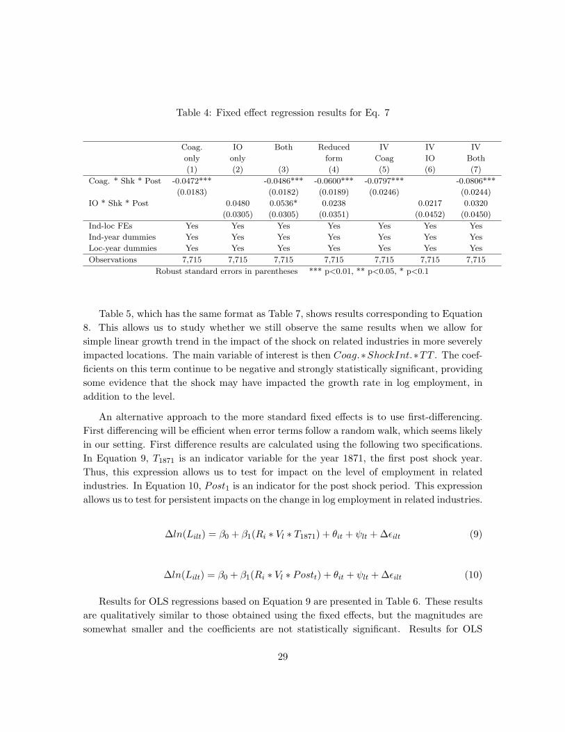
Table 4: Fixed effect regression results for Eq. 7
Coag. IO Both Reduced IV IV IV
only only form Coag IO Both
(1) (2) (3) (4) (5) (6) (7)
Coag. * Shk * Post -0.0472*** -0.0486*** -0.0600*** -0.0797*** -0.0806***
(0.0183) (0.0182) (0.0189) (0.0246) (0.0244)
IO * Shk * Post 0.0480 0.0536* 0.0238 0.0217 0.0320
(0.0305) (0.0305) (0.0351) (0.0452) (0.0450)
Ind-loc FEs Yes Yes Yes Yes Yes Yes Yes
Ind-year dummies Yes Yes Yes Yes Yes Yes Yes
Loc-year dummies Yes Yes Yes Yes Yes Yes Yes
Observations 7,715 7,715 7,715 7,715 7,715 7,715 7,715
Robust standard errors in parentheses *** p<0.01, ** p<0.05, * p<0.1
Table 5, which has the same format as Table 7, shows results corresponding to Equation8. This allows us to study whether we still observe the same results when we allow forsimple linear growth trend in the impact of the shock on related industries in more severelyimpacted locations. The main variable of interest is then Coag.∗ShockInt.∗TT . The coef-ficients on this term continue to be negative and strongly statistically significant, providingsome evidence that the shock may have impacted the growth rate in log employment, inaddition to the level.
An alternative approach to the more standard fixed effects is to use first-differencing.First differencing will be efficient when error terms follow a random walk, which seems likelyin our setting. First difference results are calculated using the following two specifications.In Equation 9, T1871 is an indicator variable for the year 1871, the first post shock year.Thus, this expression allows us to test for impact on the level of employment in relatedindustries. In Equation 10, Post1 is an indicator for the post shock period. This expressionallows us to test for persistent impacts on the change in log employment in related industries.
∆ln(Lilt) = β0 + β1(Ri ∗ Vl ∗ T1871) + θit + ψlt + ∆εilt (9)
∆ln(Lilt) = β0 + β1(Ri ∗ Vl ∗ Postt) + θit + ψlt + ∆εilt (10)
Results for OLS regressions based on Equation 9 are presented in Table 6. These resultsare qualitatively similar to those obtained using the fixed effects, but the magnitudes aresomewhat smaller and the coefficients are not statistically significant. Results for OLS
29
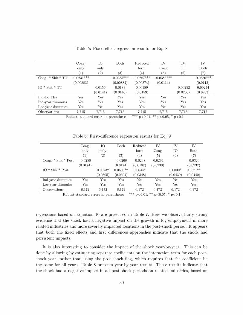
Table 5: Fixed effect regression results for Eq. 8
Coag. IO Both Reduced IV IV IV
only only form Coag IO Both
(1) (2) (3) (4) (5) (6) (7)
Coag. * Shk * TT -0.0231*** -0.0235*** -0.0287*** -0.0385*** -0.0386***
(0.00883) (0.00882) (0.00874) (0.0114) (0.0113)
IO * Shk * TT 0.0156 0.0183 0.00189 -0.00252 0.00244
(0.0141) (0.0140) (0.0159) (0.0206) (0.0203)
Ind-loc FEs Yes Yes Yes Yes Yes Yes Yes
Ind-year dummies Yes Yes Yes Yes Yes Yes Yes
Loc-year dummies Yes Yes Yes Yes Yes Yes Yes
Observations 7,715 7,715 7,715 7,715 7,715 7,715 7,715
Robust standard errors in parentheses *** p<0.01, ** p<0.05, * p<0.1
Table 6: First-difference regression results for Eq. 9
Coag. IO Both Reduced IV IV IV
only only form Coag IO Both
(1) (2) (3) (4) (5) (6) (7)
Coag. * Shk * Post -0.0250 -0.0266 -0.0238 -0.0294 -0.0320
(0.0174) (0.0174) (0.0187) (0.0238) (0.0237)
IO * Shk * Post 0.0573* 0.0603** 0.0644* 0.0830* 0.0871**
(0.0305) (0.0304) (0.0348) (0.0439) (0.0440)
Ind-year dummies Yes Yes Yes Yes Yes Yes Yes
Loc-year dummies Yes Yes Yes Yes Yes Yes Yes
Observations 6,172 6,172 6,172 6,172 6,172 6,172 6,172
Robust standard errors in parentheses *** p<0.01, ** p<0.05, * p<0.1
regressions based on Equation 10 are presented in Table 7. Here we observe fairly strongevidence that the shock had a negative impact on the growth in log employment in morerelated industries and more severely impacted locations in the post-shock period. It appearsthat both the fixed effects and first differences approaches indicate that the shock hadpersistent impacts.
It is also interesting to consider the impact of the shock year-by-year. This can bedone by allowing by estimating separate coefficients on the interaction term for each post-shock year, rather than using the post-shock flag, which requires that the coefficient bethe same for all years. Table 8 presents year-by-year results. These results indicate thatthe shock had a negative impact in all post-shock periods on related industries, based on
30
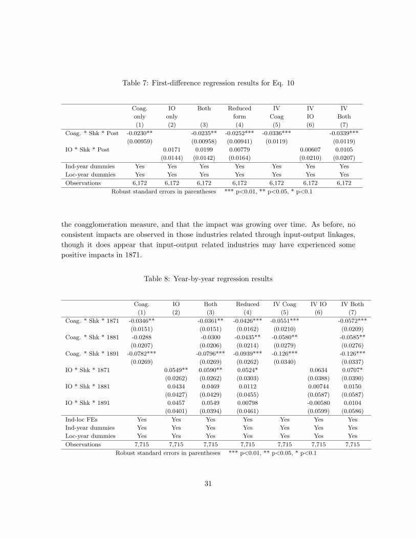
Table 7: First-difference regression results for Eq. 10
Coag. IO Both Reduced IV IV IV
only only form Coag IO Both
(1) (2) (3) (4) (5) (6) (7)
Coag. * Shk * Post -0.0230** -0.0235** -0.0252*** -0.0336*** -0.0339***
(0.00959) (0.00958) (0.00941) (0.0119) (0.0119)
IO * Shk * Post 0.0171 0.0199 0.00779 0.00607 0.0105
(0.0144) (0.0142) (0.0164) (0.0210) (0.0207)
Ind-year dummies Yes Yes Yes Yes Yes Yes Yes
Loc-year dummies Yes Yes Yes Yes Yes Yes Yes
Observations 6,172 6,172 6,172 6,172 6,172 6,172 6,172
Robust standard errors in parentheses *** p<0.01, ** p<0.05, * p<0.1
the coagglomeration measure, and that the impact was growing over time. As before, noconsistent impacts are observed in those industries related through input-output linkages,though it does appear that input-output related industries may have experienced somepositive impacts in 1871.
Table 8: Year-by-year regression results
Coag. IO Both Reduced IV Coag IV IO IV Both
(1) (2) (3) (4) (5) (6) (7)
Coag. * Shk * 1871 -0.0346** -0.0361** -0.0426*** -0.0551*** -0.0572***
(0.0151) (0.0151) (0.0162) (0.0210) (0.0209)
Coag. * Shk * 1881 -0.0288 -0.0300 -0.0435** -0.0580** -0.0585**
(0.0207) (0.0206) (0.0214) (0.0279) (0.0276)
Coag. * Shk * 1891 -0.0782*** -0.0796*** -0.0939*** -0.126*** -0.126***
(0.0269) (0.0269) (0.0262) (0.0340) (0.0337)
IO * Shk * 1871 0.0549** 0.0590** 0.0524* 0.0634 0.0707*
(0.0262) (0.0262) (0.0303) (0.0388) (0.0390)
IO * Shk * 1881 0.0434 0.0469 0.0112 0.00744 0.0150
(0.0427) (0.0429) (0.0455) (0.0587) (0.0587)
IO * Shk * 1891 0.0457 0.0549 0.00798 -0.00580 0.0104
(0.0401) (0.0394) (0.0461) (0.0599) (0.0586)
Ind-loc FEs Yes Yes Yes Yes Yes Yes Yes
Ind-year dummies Yes Yes Yes Yes Yes Yes Yes
Loc-year dummies Yes Yes Yes Yes Yes Yes Yes
Observations 7,715 7,715 7,715 7,715 7,715 7,715 7,715
Robust standard errors in parentheses *** p<0.01, ** p<0.05, * p<0.1
31
We have shown that our results tend to be robust to changes in the estimation specifica-tion. We can also check their robustness to changes to the data used to estimate the results.Table 9 presents results that assess the robustness of our findings to several changes in thedata used in the estimation. Columns (1) and (2) present results calculated when data fromLiverpool is included. Column (1) presents fixed effects results including both relatednessmeasures, and column (2) presents IV results. Recall that Liverpool was excluded becauseindustries other than cotton textiles were directly impacted by the civil war there. IncludingLiverpool does not appear to alter our results.
Another potential issue arises from the fact that the set of towns used to obtain ourresults may also influence the coagglomeration measure. To see why this might cause anissue, suppose that the coagglomeration measure simply reflects a random chance that anindustry ends up coagglomerated with cotton textiles, rather than underlying connectionsbetween these industries. Furthermore, suppose that when cotton textiles is shocked ina location all industries in that location suffer, with the industries more agglomerated inthe location suffering more. This scenario may cause errant results if the coagglomerationmeasure is driven by the towns used in our analysis. This is unlikely because we havecalculated coagglomeration using district-level, rather than town-level data, which coversmany areas other than the towns used in the analysis. However, if one is still worried thatthe towns used are driving the coagglomeration measure, then results can be recalculatedusing a coagglomeration measure calculated using only districts that do not include townsused in the subsequent analysis. Results using this alternative coagglomeration measureare presented columns (3) and (4) of Table 9.
Columns (5) and (6) of Table 9 presents results when all wool-related industries havebeen dropped from the analysis. While these are an important class of industries whichare closely related to the cotton textile industry, we may be worried that the fact thatthey are initially much larger in Yorkshire towns could lead them to grow faster there,in the presence of economies of scale or within-industry spillovers. While dropping theseindustries does reduce the size of the estimated impact, it does not alter the basic message.Finally, columns (7) and (8) include results in which all industries sharing intermediategood input-output connections with the cotton textile industry have been excluded fromthe analysis. This appears to strengthen our results, providing further evidence that theobserved impacts were not driven by intermediate goods input-output connections.
Three innovations offered by this study, vis a vis existing studies, is the use of geograph-ically disaggregated data, the use of more detailed industry-level data, and accounting forthe pattern of inter-industry connections. Given that our results differ from previous studieswhich find that temporary shocks have few long-term impacts, such as Davis & Weinstein(2008), it is interesting to look at which of these innovations appears to be driving our
32
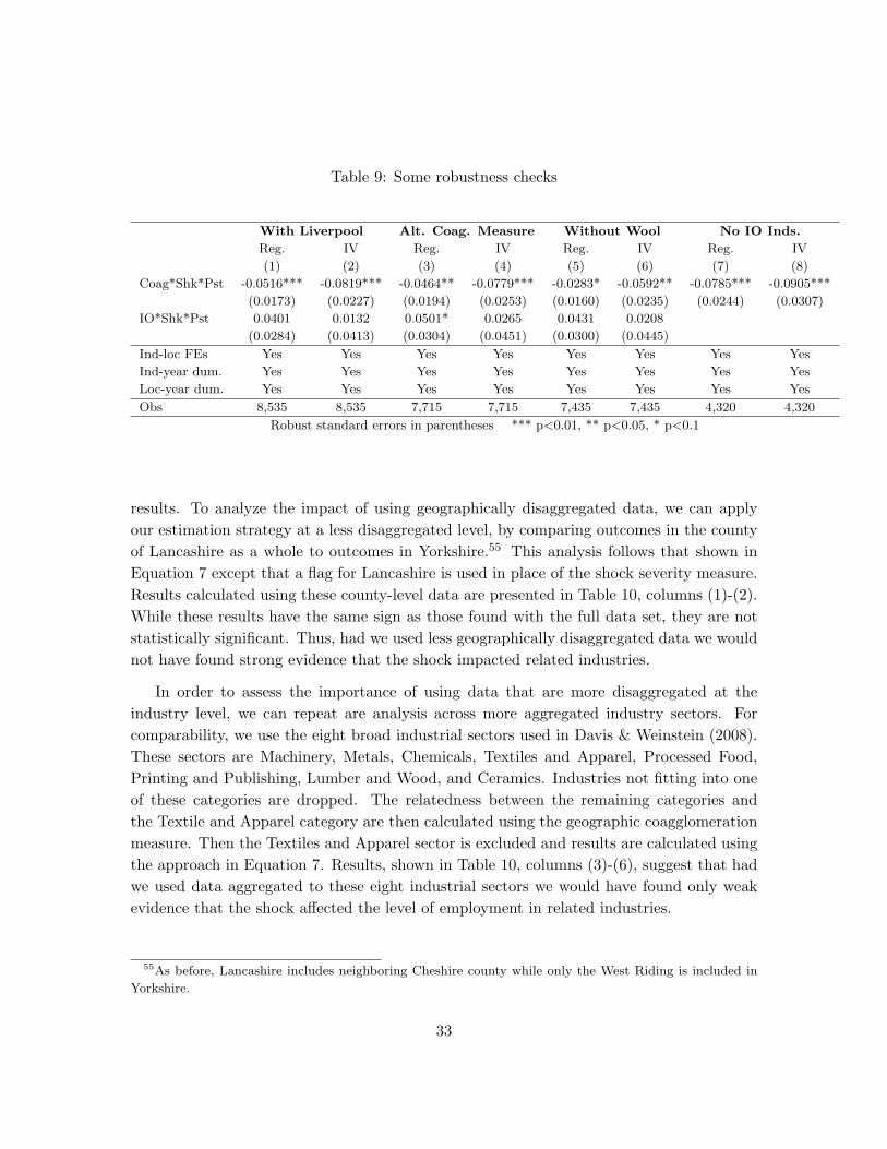
Table 9: Some robustness checks
With Liverpool Alt. Coag. Measure Without Wool No IO Inds.
Reg. IV Reg. IV Reg. IV Reg. IV
(1) (2) (3) (4) (5) (6) (7) (8)
Coag*Shk*Pst -0.0516*** -0.0819*** -0.0464** -0.0779*** -0.0283* -0.0592** -0.0785*** -0.0905***
(0.0173) (0.0227) (0.0194) (0.0253) (0.0160) (0.0235) (0.0244) (0.0307)
IO*Shk*Pst 0.0401 0.0132 0.0501* 0.0265 0.0431 0.0208
(0.0284) (0.0413) (0.0304) (0.0451) (0.0300) (0.0445)
Ind-loc FEs Yes Yes Yes Yes Yes Yes Yes Yes
Ind-year dum. Yes Yes Yes Yes Yes Yes Yes Yes
Loc-year dum. Yes Yes Yes Yes Yes Yes Yes Yes
Obs 8,535 8,535 7,715 7,715 7,435 7,435 4,320 4,320
Robust standard errors in parentheses *** p<0.01, ** p<0.05, * p<0.1
results. To analyze the impact of using geographically disaggregated data, we can applyour estimation strategy at a less disaggregated level, by comparing outcomes in the countyof Lancashire as a whole to outcomes in Yorkshire.55 This analysis follows that shown inEquation 7 except that a flag for Lancashire is used in place of the shock severity measure.Results calculated using these county-level data are presented in Table 10, columns (1)-(2).While these results have the same sign as those found with the full data set, they are notstatistically significant. Thus, had we used less geographically disaggregated data we wouldnot have found strong evidence that the shock impacted related industries.
In order to assess the importance of using data that are more disaggregated at theindustry level, we can repeat are analysis across more aggregated industry sectors. Forcomparability, we use the eight broad industrial sectors used in Davis & Weinstein (2008).These sectors are Machinery, Metals, Chemicals, Textiles and Apparel, Processed Food,Printing and Publishing, Lumber and Wood, and Ceramics. Industries not fitting into oneof these categories are dropped. The relatedness between the remaining categories andthe Textile and Apparel category are then calculated using the geographic coagglomerationmeasure. Then the Textiles and Apparel sector is excluded and results are calculated usingthe approach in Equation 7. Results, shown in Table 10, columns (3)-(6), suggest that hadwe used data aggregated to these eight industrial sectors we would have found only weakevidence that the shock affected the level of employment in related industries.
55As before, Lancashire includes neighboring Cheshire county while only the West Riding is included in
Yorkshire.
33
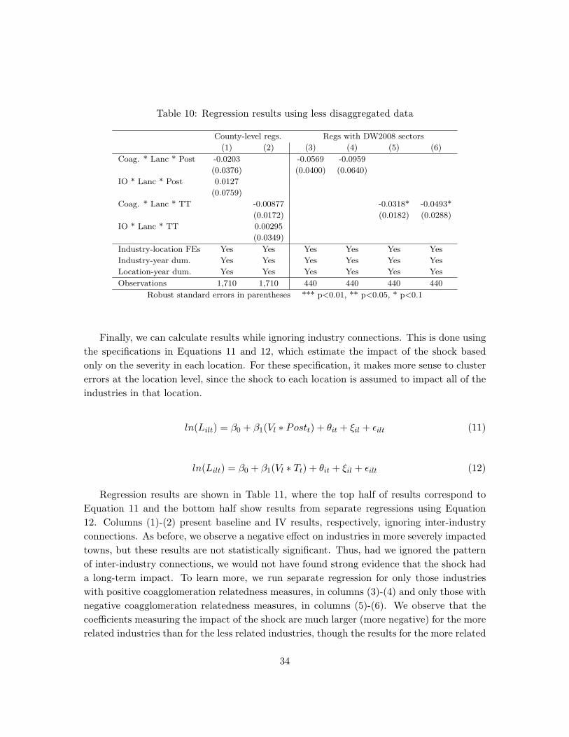
Table 10: Regression results using less disaggregated data
County-level regs. Regs with DW2008 sectors
(1) (2) (3) (4) (5) (6)
Coag. * Lanc * Post -0.0203 -0.0569 -0.0959
(0.0376) (0.0400) (0.0640)
IO * Lanc * Post 0.0127
(0.0759)
Coag. * Lanc * TT -0.00877 -0.0318* -0.0493*
(0.0172) (0.0182) (0.0288)
IO * Lanc * TT 0.00295
(0.0349)
Industry-location FEs Yes Yes Yes Yes Yes Yes
Industry-year dum. Yes Yes Yes Yes Yes Yes
Location-year dum. Yes Yes Yes Yes Yes Yes
Observations 1,710 1,710 440 440 440 440
Robust standard errors in parentheses *** p<0.01, ** p<0.05, * p<0.1
Finally, we can calculate results while ignoring industry connections. This is done usingthe specifications in Equations 11 and 12, which estimate the impact of the shock basedonly on the severity in each location. For these specification, it makes more sense to clustererrors at the location level, since the shock to each location is assumed to impact all of theindustries in that location.
ln(Lilt) = β0 + β1(Vl ∗ Postt) + θit + ξil + εilt (11)
ln(Lilt) = β0 + β1(Vl ∗ Tt) + θit + ξil + εilt (12)
Regression results are shown in Table 11, where the top half of results correspond toEquation 11 and the bottom half show results from separate regressions using Equation12. Columns (1)-(2) present baseline and IV results, respectively, ignoring inter-industryconnections. As before, we observe a negative effect on industries in more severely impactedtowns, but these results are not statistically significant. Thus, had we ignored the patternof inter-industry connections, we would not have found strong evidence that the shock hada long-term impact. To learn more, we run separate regression for only those industrieswith positive coagglomeration relatedness measures, in columns (3)-(4) and only those withnegative coagglomeration relatedness measures, in columns (5)-(6). We observe that thecoefficients measuring the impact of the shock are much larger (more negative) for the morerelated industries than for the less related industries, though the results for the more related
34
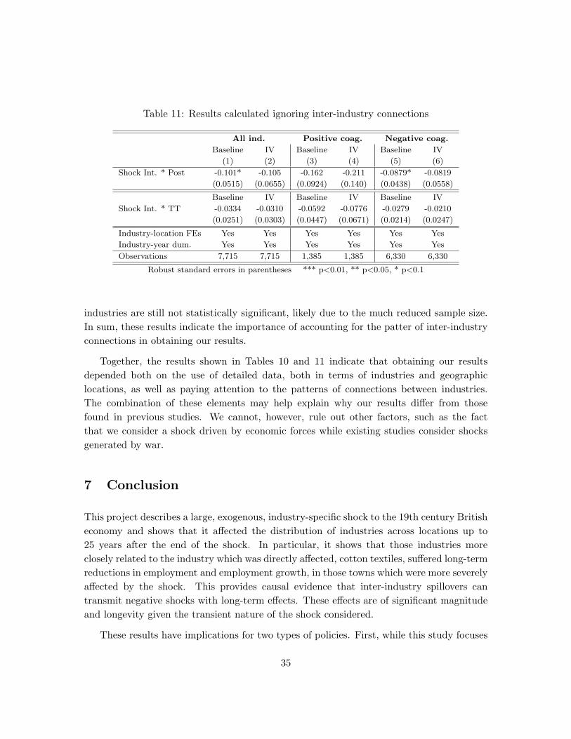
Table 11: Results calculated ignoring inter-industry connections
All ind. Positive coag. Negative coag.
Baseline IV Baseline IV Baseline IV
(1) (2) (3) (4) (5) (6)
Shock Int. * Post -0.101* -0.105 -0.162 -0.211 -0.0879* -0.0819
(0.0515) (0.0655) (0.0924) (0.140) (0.0438) (0.0558)
Baseline IV Baseline IV Baseline IV
Shock Int. * TT -0.0334 -0.0310 -0.0592 -0.0776 -0.0279 -0.0210
(0.0251) (0.0303) (0.0447) (0.0671) (0.0214) (0.0247)
Industry-location FEs Yes Yes Yes Yes Yes Yes
Industry-year dum. Yes Yes Yes Yes Yes Yes
Observations 7,715 7,715 1,385 1,385 6,330 6,330
Robust standard errors in parentheses *** p<0.01, ** p<0.05, * p<0.1
industries are still not statistically significant, likely due to the much reduced sample size.In sum, these results indicate the importance of accounting for the patter of inter-industryconnections in obtaining our results.
Together, the results shown in Tables 10 and 11 indicate that obtaining our resultsdepended both on the use of detailed data, both in terms of industries and geographiclocations, as well as paying attention to the patterns of connections between industries.The combination of these elements may help explain why our results differ from thosefound in previous studies. We cannot, however, rule out other factors, such as the factthat we consider a shock driven by economic forces while existing studies consider shocksgenerated by war.
7 Conclusion
This project describes a large, exogenous, industry-specific shock to the 19th century Britisheconomy and shows that it affected the distribution of industries across locations up to25 years after the end of the shock. In particular, it shows that those industries moreclosely related to the industry which was directly affected, cotton textiles, suffered long-termreductions in employment and employment growth, in those towns which were more severelyaffected by the shock. This provides causal evidence that inter-industry spillovers cantransmit negative shocks with long-term effects. These effects are of significant magnitudeand longevity given the transient nature of the shock considered.
These results have implications for two types of policies. First, while this study focuses
35

on a large negative shock caused by exogenous factors, it seems possible that localizedindustrial policy interventions may be able to generate similar effects. This may providesome justification for the widespread use of these policies. However, these results alsosuggest that the effectiveness of such policy interventions depends crucially on the patternof connections between industries, which are currently not well understood.
These results also have implications for policies that may influence the vulnerability ofan economy to economic shocks, because they suggest that even temporary shocks, if largeenough, can have long-lasting effects. While this study shows how a temporary shock canreallocate industries within a country, the same forces are also likely to be at work acrosscountries. Thus, policy makers may want to consider the potential effects of volatility whenconsidering policies that increase and economy’s vulnerability to temporary shocks.
While this study tells us that inter-industry connections can transmit economic forcesbetween industries, with long-term implications, we are unable to identify the particulartypes of connections that are most important, though it does not appear that intermediategood input-output linkages are driving the observed results. More clearly identifying theparticular types of industries that drive the effects we observe is an important direction forfuture research.
36
References
Aitken, BJ, & Harrison, AE. 1999. Do domestic firms benefit from direct foreign investment? Evidence from
Venezuela. American Economic Review , 89(3), 605–618.
Allen, RC. 2009. The British Industrial Revolution in Global Perspective. Cambridge University Press.
Amiti, M, & Cameron, L. 2007. Economic Geography and Wages. Review of Economics and Statistics,
89(1), pp. 15–29.
Angrist, J., & Pischke, JS. 2009. Mostly Harmless Econometrics: An Empiricists Companion. Princeton
University Press.
Arnold, A. 1864. The History of The Cotton Famine: From the Fall of Sumter to the Passing of The Public
Works Act. London: Saunders, Otley, and Co.
Arrow, KJ. 1962. The Economic Implications of Learning by Doing. The Review of Economic Studies, 29(3),
155–173.
Arzaghi, M, & Henderson, JV. 2008. Networking off Madison Avenue. Review of Economic Studies, 75, pp.
1011–1038.
Balsvik, R. Forthcoming. Is labor mobility a channel for spillovers from multinationals? Evidence from
Norwegian manufacturing. Review of Economics and Statistics.
Bertrand, M., Duflo, E., & Mullainathan, S. 2004. How Much Should We Trust Differences-in-Differences
Estimates? The Quarterly Journal of Economics, 119(1), pp. 249–275.
Bloom, N, Schankerman, M, & Van Reenen, J. 2007 (Apr.). Identifying Technology Spillovers and Product
Market Rivalry.
Bosker, M, Brakman, S, Garretsen, H, & Schramm, M. 2008a. A Century of Shocks: The Evolution of the
German City Size Distribution 1925-1999. Regional Science and Urban Economics, 38(4), pp. 330–347.
Bosker, M, Brakman, S, Garretsen, H, De Jong, H, & Schramm, M. 2008b. Ports, Plagues, and Politics:
Explaining Italian City Growth 1300-1861. European Review of Economic History, 12, pp. 97–131.
Bosker, Maarten, Brakman, Steven, Garretsen, Harry, & Schramm, Marc. 2007. Looking for multiple equi-
libria when geography matters: German city growth and the WWII shock. Journal of Urban Economics,
61(1), 152 – 169.
Bottazzi, L, & Peri, G. 2003. Innovation and spillovers in regions: Evidence from European patent data.
European Economic Review, 47(4), 687–710.
Brakman, S., Garretsen, H, & Schramm, M. 2004. The Strategic Bombing of German Cities During WWII
and its Impact on City Growth. Journal of Economic Geography, 4, pp. 201–218.
Catling, H. 1986. The Spinning Mule. Lancashire: Lancashire County Council Library and Leisure Com-
mittee.
Ciccone, A. 2002. Input Chains and Industrialization. Review of Economic Studies, 69, pp. 565–587.
Ciccone, A. 2007. Linkages.
Davis, Donald R., & Weinstein, David E. 2008. A search for multiple equilibria in urban industrial structure.
Journal of Regional Science, 48(1), 29–65.
Davis, DR, & Weinstein, DE. 2002. Bones, bombs, and break points: The geography of economic activity.
American Economic Review, 92(5), 1269–1289.
Deane, P., & Cole, WA. 1967. British Economic Growth. Cambridge, UK: Cambridge University Press.
di Giovanni, Julian, & Levchenko, Andrei A. 2009. Trade Openness and Volatility. Review of Economics
and Statistics, 91(3), 558 – 585.
Donald, S, & Lang, K. 2007. Inference with Difference-in-Differences and Other Panel Data. The Review of
Economics and Statistics, 89(2), pp. 221–233.
Donaldson, D. 2010. Railroads and the Raj: Estimating the Impact of Transportation Infrastructure. Working
paper.
Ellison, G, & Glaeser, EL. 1997. Geographic concentration in US manufacturing industries: A dartboard
37
approach. Journal of Political Economy, 105(5), 889–927.
Ellison, G., Glaeser, E., & Kerr, W. 2010. What Causes Industry Agglomeration? Evidence from Coag-
glomeration Patterns. American Economic Review, 100(3), pp. 1195–1213.
Farnie, D. 2004. The Role of the Cotton Industry in Economic Development. Oxford University Press.
Chap. 18, pages pp. 557–584.
Feenstra, R. 1996. Trade and Uneven Growth. Journal of Development Economics, 49, pp. 229–265.
Forwood, William B. 1870. The Influence of Price upon the Cultivation and Consumption of Cotton During
the Ten Years 1860-70. Journal of the Statistical Society of London, 33(3), 366–383.
Fujita, M., Krugman, P., & Venables, A. 1999. The Spatial Economy: Cities, Regions, and International
Trade. Cambridge: The MIT Press.
Glaeser, EL, Kallal, HD, Scheinkman, JA, & Shleifer, A. 1992. Growth in Cities. Journal of Political
Economy, 100(6), 1126–1152.
Greenstone, M, & Moretti, E. 2004. Bidding for Industrial Plants: Does Winning a ‘Million Dollar Plant’
Increase Welfare? MIT Department of Economics Working Paper No. 04-39.
Greenstone, M., Hornbeck, R., & Moretti, E. 2010. Identifying Agglomeration Spillovers: Evidence from
Million Dollar Plants. Journal of Political Economy, 118(3), pp. 536–598.
Grossman, G, & Helpman, E. 1990. Comparative Advantage and Long-Run Growth. American Economic
Review, 80(4), pp. 796–815.
Helm, E. 1869. A Review of the Cotton Trade of the United Kingdom, during the Seven Years, 1862-1868.
Transactions of the Manchester Statistical Society 1868-1869, pp. 67–94.
Helsley, Robert W, & Strange, William C. 2010 (Nov.). Coagglomeration. Working paper.
Henderson, JV. 2003. Marshall’s Scale Economies. Journal of Urban Economics , 53(1), 1–28.
Henderson, V. 1997. Externalities and industrial development. Journal of Urban Economics, 42(3), 449–470.
Henderson, WO. 1969. The Lancashire Cotton Famine 1861-1865. New York: Augustus M. Kelley Publishers.
Hirschman, AO. 1958. The Strategy of Economic Development. New Haven, CN: Yale University Press.
Horrell, S., Humphries, J., & Weale, M. 1994. An Input-Output Table for 1841. Economic History Review,
47(3), 545–566.
Jacobs, J. 1969. The Economy of Cities. New York: Vintage Books.
Javorcik, BS. 2004. Does Foreign Direct Investment Increase the Productivity of Domestic Firms? In Search
of Spillovers through Backward Linkages. The American Economic Review, 94(3), 605–627.
Jenkins, DT, & Ponting, KG. 1987. The British Wool Textile Industry, 1770-1914. Aldershop, UK: Scolar
Press.
Kim, S. 1995. Expansion of Markets and the Geographic Distribution of Economic Activities - The Trends
in US Regional Manufacturing Structure, 1860-1987. Quarterly Journal of Economics , 110(4), 881–908.
Krugman, P. 1991. Increasing Returns and Economic Geography. Journal of Political Economy, 99(3), pp.
483–499.
Krugman, P., & Venables, A. 1995. Globalization and the Inequality of Nations. Quarterly Journal of
Economics, 110(4), pp. 857–880.
Kugler, M. 2006. Spillovers from foreign direct investment: Within or between industries? Journal of
Development Economics, 80(2), 444–477.
Lazonick, W. 1990. Competitive Advantage on the Shop Floor. Cambridge, MA: Harvard University Press.
Lee, C. 1979. British Regional Employment Statistics 1841-1971. Cambridge, UK: Cambridge University
Press.
Lucas, RE. 1988. On the Mechanics of Economic Development. Journal of Monetary Economics, 22(1),
3–42.
Marshall, A. 1890. Principles of Economics. New York: Macmillan and Co.
Marshall, Alfred. 1920. Principles of Economics: An Introductory Volume. 8th edn. London: Macmillan.
38

Matsuyama, K. 1992. Agricultural Productivity, Comparative Advantage, and Economic Growth . Journal
of Economic Theory, 58(2), 317–334.
McCloskey, D. 1994. 1700-1860: A Survey. Pages 242–270 of: Floud, R., & McCloskey, D. (eds), The
Economic History of Britain Since 1700 Volume 1. Cambridge, UK: Cambridge University Press.
Miguel, E, & Roland, G. 2006 (Jan.). The Long Run Impact of Bombing Vietnam.
Mitchell, BR. 1988. British Historical Statistics. Cambridge, UK: Cambridge University Press.
Mitchell, BR, & Deane, P. 1962. Abstract of British Historical Statistics. London: Cambridge University
Press.
Mokyr, J. 1985. The Industrial Revolution and the New Economic History. Rowman & Littlefield Publishers,
Inc. In The Economics of the Industrial Revolution. Pages pp. 1–51.
Ollerenshaw, JC. 1870. Our Export Trade in Cotton Goods to India. Transactions of the Manchester
Statistical Society, 1869-1870, p. 112.
Poole, J. 2009. Knowledge Transfers from Multinational to Domestic Firms: Evidence from Worker Mobility.
Working paper.
Porter, ME. 1990. The Competitive Advantage of Nations. New York, NY: The Free Press.
Redding, S, Sturm, D, & Wolf, N. forthcoming. History and Industry Location: Evidence from German
Airports. Review of Economics and Statistics.
Rivera-Batiz, LA, & Romer, PM. 1991. International Trade with Endogenous Technological Change. Euro-
pean Economic Review, 35(4), 971–1004.
Rodrıguez-Clare, Andres. 1996. Multinationals, linkages, and economic development. American Economic
Review, 86(4), 852–873.
Rodriguez, F, & Rodrik, D. 2000. Trade policy and economic growth: A skeptic’s guide to the cross-national
evidence. NBER Macroeconomics Annual, 15, 261–325.
Rosenthal, SS, & Strange, WC. 2001. The Determinants of Agglomeration. Journal of Urban Economics ,
50(2), 191–229.
Rostow, WW. 1960. The Stages of Economic Growth. Cambridge University Press.
Southall, H. 1991. Poor Law Statistics and the Geography of Economic Distress. Cambridge University
Press. Chap. 7, pages 180–217.
Southall, HR, Gilbert, DR, & Gregory, I. 1998 (Jan.). Great Britain Historical Database : Labour Markets
Database, Poor Law Statistics, 1859-1939. [computer file]. UK Data Archive [distributor] SN: 3713.
Thomas, M. 1987. An Input-Output Approach to the British Economy, 1890-1914. Ph.D. thesis, Oxford
University.
Timmins, G. 1998. Made in Lancashire: A History of Regional Industrialization. Manchester, England:
Manchester University Press.
Woolard, M. 1999. The Classification of Occupations in the 1881 Census of England and Wales. Mimeo.
Young, A. 1991. Learning By Doing and the Dynamic Effects of International Trade . Quarterly Journal of
Economics , 106(2), 369–405.
39
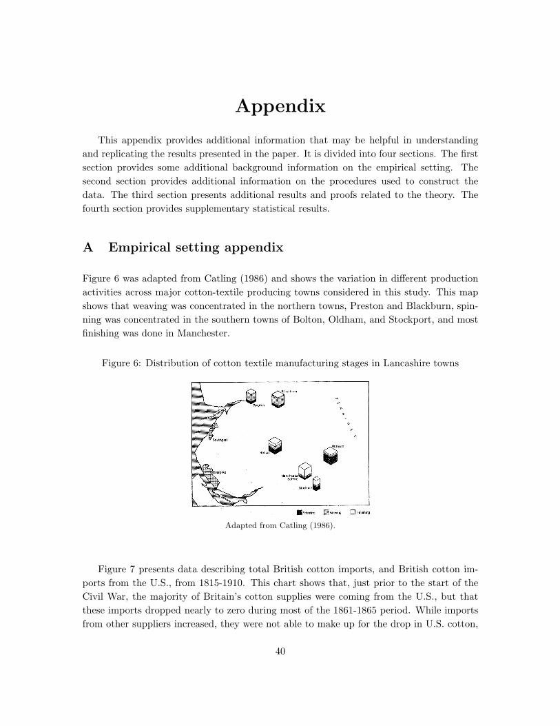
Appendix
This appendix provides additional information that may be helpful in understandingand replicating the results presented in the paper. It is divided into four sections. The firstsection provides some additional background information on the empirical setting. Thesecond section provides additional information on the procedures used to construct thedata. The third section presents additional results and proofs related to the theory. Thefourth section provides supplementary statistical results.
A Empirical setting appendix
Figure 6 was adapted from Catling (1986) and shows the variation in different productionactivities across major cotton-textile producing towns considered in this study. This mapshows that weaving was concentrated in the northern towns, Preston and Blackburn, spin-ning was concentrated in the southern towns of Bolton, Oldham, and Stockport, and mostfinishing was done in Manchester.
Figure 6: Distribution of cotton textile manufacturing stages in Lancashire towns
Adapted from Catling (1986).
Figure 7 presents data describing total British cotton imports, and British cotton im-ports from the U.S., from 1815-1910. This chart shows that, just prior to the start of theCivil War, the majority of Britain’s cotton supplies were coming from the U.S., but thatthese imports dropped nearly to zero during most of the 1861-1865 period. While importsfrom other suppliers increased, they were not able to make up for the drop in U.S. cotton,
40
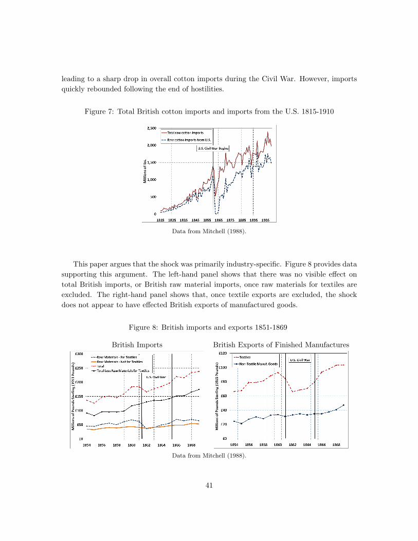
leading to a sharp drop in overall cotton imports during the Civil War. However, importsquickly rebounded following the end of hostilities.
Figure 7: Total British cotton imports and imports from the U.S. 1815-1910
Data from Mitchell (1988).
This paper argues that the shock was primarily industry-specific. Figure 8 provides datasupporting this argument. The left-hand panel shows that there was no visible effect ontotal British imports, or British raw material imports, once raw materials for textiles areexcluded. The right-hand panel shows that, once textile exports are excluded, the shockdoes not appear to have effected British exports of manufactured goods.
Figure 8: British imports and exports 1851-1869
British Imports British Exports of Finished Manufactures
Data from Mitchell (1988).
41
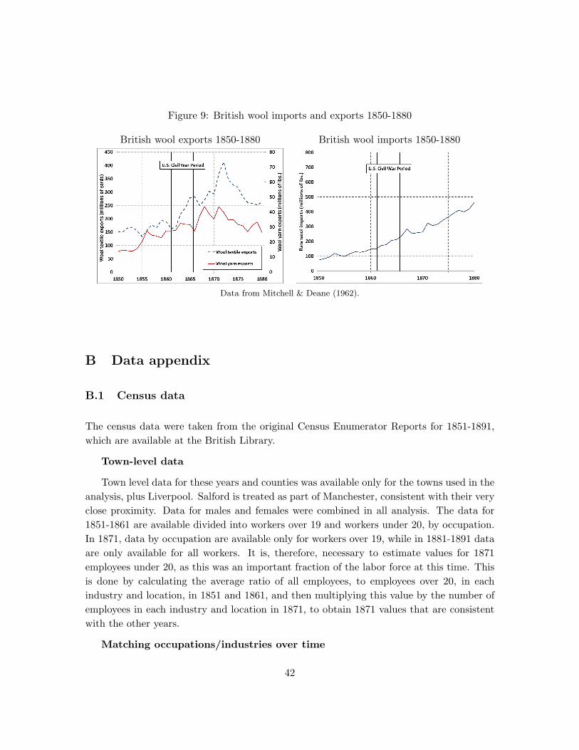
Figure 9: British wool imports and exports 1850-1880
British wool exports 1850-1880 British wool imports 1850-1880
Data from Mitchell & Deane (1962).
B Data appendix
B.1 Census data
The census data were taken from the original Census Enumerator Reports for 1851-1891,which are available at the British Library.
Town-level data
Town level data for these years and counties was available only for the towns used in theanalysis, plus Liverpool. Salford is treated as part of Manchester, consistent with their veryclose proximity. Data for males and females were combined in all analysis. The data for1851-1861 are available divided into workers over 19 and workers under 20, by occupation.In 1871, data by occupation are available only for workers over 19, while in 1881-1891 dataare only available for all workers. It is, therefore, necessary to estimate values for 1871employees under 20, as this was an important fraction of the labor force at this time. Thisis done by calculating the average ratio of all employees, to employees over 20, in eachindustry and location, in 1851 and 1861, and then multiplying this value by the number ofemployees in each industry and location in 1871, to obtain 1871 values that are consistentwith the other years.
Matching occupations/industries over time
42
Industry categories changed over time, so it was necessary to combine multiple industriesin order to construct more consistent industry groupings over the study period. Individ-ual categories in the years were combined into industry groups based on (1) the census’occupation classes and (2) the name of the occupation. For some occupations, it was notpossible to form consistent groups over all years, and these occupations are omitted fromthe analysis. It is still the case that some occupation groups may not be perfectly consistentover time, however, because our identification strategy controls for aggregate industry-yeareffects, it should be less affected by this source of measurement error. The occupationalcategories prior to 1851 and after 1891 change significantly, relative to the period that westudy, which motivates our choice of study period.
Calculating geographic coagglomeration
The measure of geographic coagglomeration is based on Ellison et al. (2010) and is cal-culated using data from 71 district within Lancashire. The use of data from only Lancashirehere is important. There are two good reasons for taking this approach. First, it is thepattern of relatedness in Lancashire that determines which industries are affected by theshock. Thus far, little is known about the extent to which deep patterns of industry relat-edness vary across locations. Using only one location minimizes this concern. Second, thereis a danger in calculating coagglomeration measures over too broad an area. To see why,consider some industry x which is related to both the cotton and wool textile industriesand is coagglomerated with cotton textiles in Lancashire and wool textiles in Yorkshire.If the coagglomeration measures is calculated using only Lancashire county, we find thatindustry x is coagglomerated with cotton textiles. If data from Yorkshire are added, therewill be a sharp reduction in the level of coagglomeration of industry x with cotton textiles,because there are now concentrations of industry x in Yorkshire districts with very littlecotton textile production (but a lot of wool textile production). To calculate the measure,we suppose that there are M districts, and let smi be the share of industry i’s employmentin some district m. Let xm be district m’s share of workers. Geographic coagglomerationbetween industries i and j is given by Rij , where,
Rij =∑Mm=1(smi − xm)(smj − xm)
1−∑Mm=1 x
2m
Table 12 gives the fifteen most and least related industries to the cotton textile industry,according to the coagglomeration measure. Note that, for illustration, this table includescotton-based industries which are later excluded from the analysis.
43
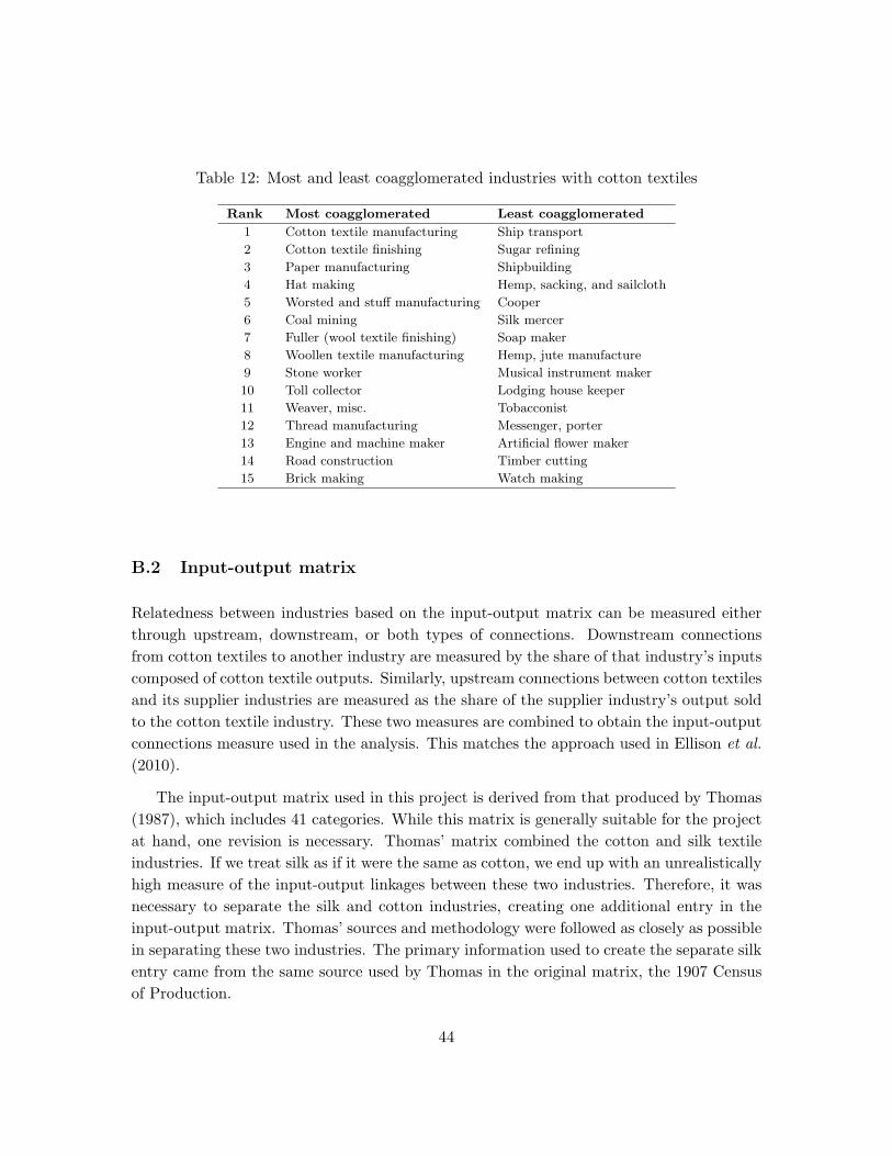
Table 12: Most and least coagglomerated industries with cotton textiles
Rank Most coagglomerated Least coagglomerated
1 Cotton textile manufacturing Ship transport
2 Cotton textile finishing Sugar refining
3 Paper manufacturing Shipbuilding
4 Hat making Hemp, sacking, and sailcloth
5 Worsted and stuff manufacturing Cooper
6 Coal mining Silk mercer
7 Fuller (wool textile finishing) Soap maker
8 Woollen textile manufacturing Hemp, jute manufacture
9 Stone worker Musical instrument maker
10 Toll collector Lodging house keeper
11 Weaver, misc. Tobacconist
12 Thread manufacturing Messenger, porter
13 Engine and machine maker Artificial flower maker
14 Road construction Timber cutting
15 Brick making Watch making
B.2 Input-output matrix
Relatedness between industries based on the input-output matrix can be measured eitherthrough upstream, downstream, or both types of connections. Downstream connectionsfrom cotton textiles to another industry are measured by the share of that industry’s inputscomposed of cotton textile outputs. Similarly, upstream connections between cotton textilesand its supplier industries are measured as the share of the supplier industry’s output soldto the cotton textile industry. These two measures are combined to obtain the input-outputconnections measure used in the analysis. This matches the approach used in Ellison et al.(2010).
The input-output matrix used in this project is derived from that produced by Thomas(1987), which includes 41 categories. While this matrix is generally suitable for the projectat hand, one revision is necessary. Thomas’ matrix combined the cotton and silk textileindustries. If we treat silk as if it were the same as cotton, we end up with an unrealisticallyhigh measure of the input-output linkages between these two industries. Therefore, it wasnecessary to separate the silk and cotton industries, creating one additional entry in theinput-output matrix. Thomas’ sources and methodology were followed as closely as possiblein separating these two industries. The primary information used to create the separate silkentry came from the same source used by Thomas in the original matrix, the 1907 Censusof Production.
44
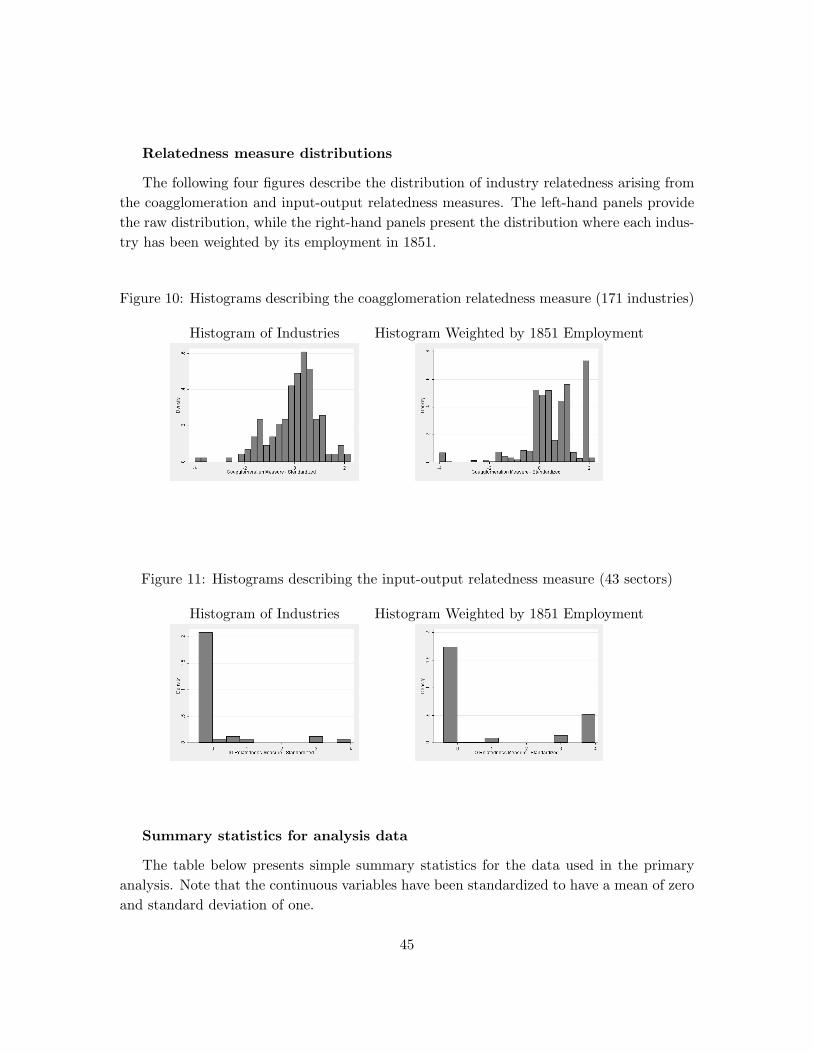
Relatedness measure distributions
The following four figures describe the distribution of industry relatedness arising fromthe coagglomeration and input-output relatedness measures. The left-hand panels providethe raw distribution, while the right-hand panels present the distribution where each indus-try has been weighted by its employment in 1851.
Figure 10: Histograms describing the coagglomeration relatedness measure (171 industries)
Histogram of Industries Histogram Weighted by 1851 Employment
Figure 11: Histograms describing the input-output relatedness measure (43 sectors)
Histogram of Industries Histogram Weighted by 1851 Employment
Summary statistics for analysis data
The table below presents simple summary statistics for the data used in the primaryanalysis. Note that the continuous variables have been standardized to have a mean of zeroand standard deviation of one.
45
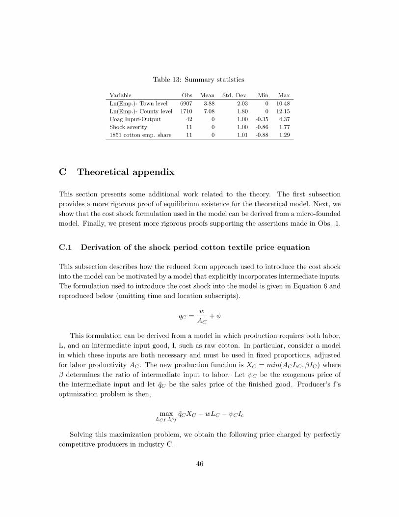
Table 13: Summary statistics
Variable Obs Mean Std. Dev. Min Max
Ln(Emp.)- Town level 6907 3.88 2.03 0 10.48
Ln(Emp.)- County level 1710 7.08 1.80 0 12.15
Coag Input-Output 42 0 1.00 -0.35 4.37
Shock severity 11 0 1.00 -0.86 1.77
1851 cotton emp. share 11 0 1.01 -0.88 1.29
C Theoretical appendix
This section presents some additional work related to the theory. The first subsectionprovides a more rigorous proof of equilibrium existence for the theoretical model. Next, weshow that the cost shock formulation used in the model can be derived from a micro-foundedmodel. Finally, we present more rigorous proofs supporting the assertions made in Obs. 1.
C.1 Derivation of the shock period cotton textile price equation
This subsection describes how the reduced form approach used to introduce the cost shockinto the model can be motivated by a model that explicitly incorporates intermediate inputs.The formulation used to introduce the cost shock into the model is given in Equation 6 andreproduced below (omitting time and location subscripts).
qC =w
AC+ φ
This formulation can be derived from a model in which production requires both labor,L, and an intermediate input good, I, such as raw cotton. In particular, consider a modelin which these inputs are both necessary and must be used in fixed proportions, adjustedfor labor productivity AC . The new production function is XC = min(ACLC , βIC) whereβ determines the ratio of intermediate input to labor. Let ψC be the exogenous price ofthe intermediate input and let qC be the sales price of the finished good. Producer’s f’soptimization problem is then,
maxLCf ,ICf
qCXC − wLC − ψCIc
Solving this maximization problem, we obtain the following price charged by perfectlycompetitive producers in industry C.
46
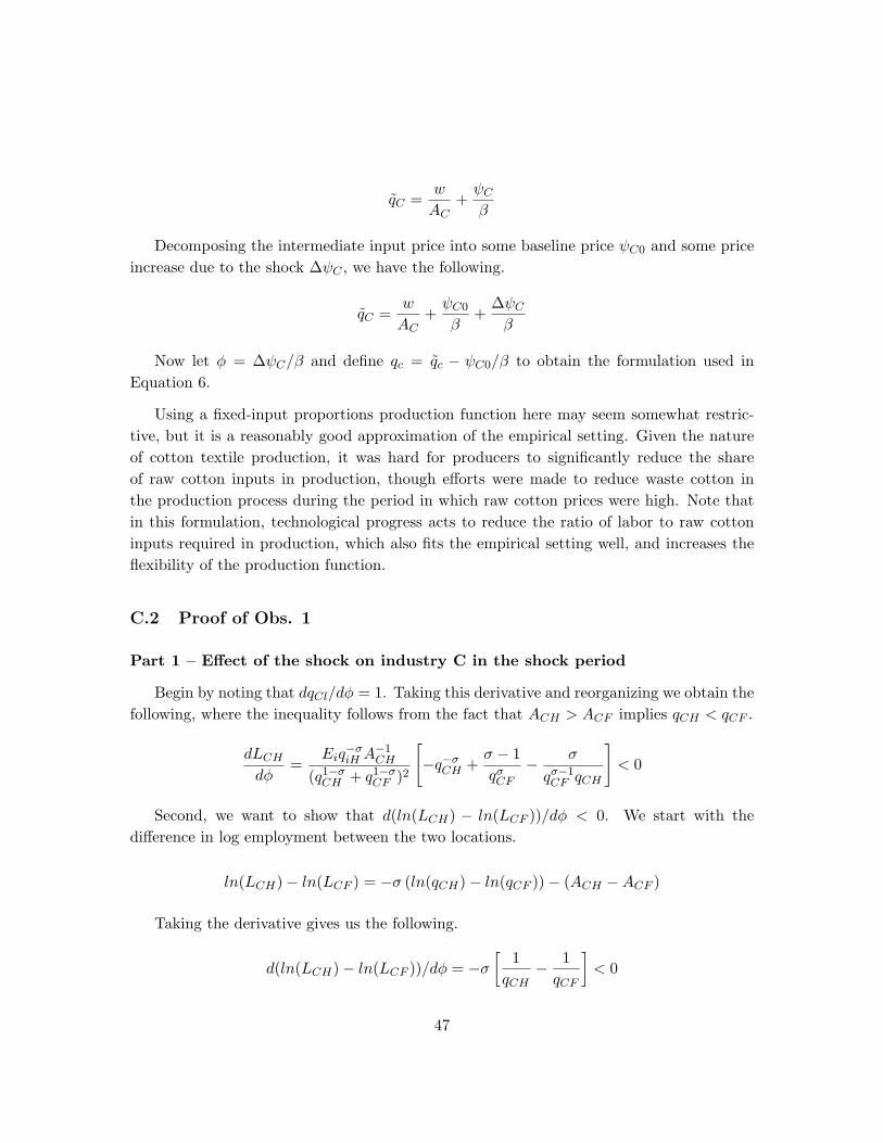
qC =w
AC+ψCβ
Decomposing the intermediate input price into some baseline price ψC0 and some priceincrease due to the shock ∆ψC , we have the following.
qC =w
AC+ψC0
β+
∆ψCβ
Now let φ = ∆ψC/β and define qc = qc − ψC0/β to obtain the formulation used inEquation 6.
Using a fixed-input proportions production function here may seem somewhat restric-tive, but it is a reasonably good approximation of the empirical setting. Given the natureof cotton textile production, it was hard for producers to significantly reduce the shareof raw cotton inputs in production, though efforts were made to reduce waste cotton inthe production process during the period in which raw cotton prices were high. Note thatin this formulation, technological progress acts to reduce the ratio of labor to raw cottoninputs required in production, which also fits the empirical setting well, and increases theflexibility of the production function.
C.2 Proof of Obs. 1
Part 1 – Effect of the shock on industry C in the shock period
Begin by noting that dqCl/dφ = 1. Taking this derivative and reorganizing we obtain thefollowing, where the inequality follows from the fact that ACH > ACF implies qCH < qCF .
dLCHdφ
=Eiq−σiH A
−1CH
(q1−σCH + q1−σCF )2
[−q−σCH +
σ − 1qσCF
− σ
qσ−1CF qCH
]< 0
Second, we want to show that d(ln(LCH) − ln(LCF ))/dφ < 0. We start with thedifference in log employment between the two locations.
ln(LCH)− ln(LCF ) = −σ (ln(qCH)− ln(qCF ))− (ACH −ACF )
Taking the derivative gives us the following.
d(ln(LCH)− ln(LCF ))/dφ = −σ[
1qCH
− 1qCF
]< 0
47
C.3 Proof of Obs. 3
We must show that when τ iC > 0 and ACH > ACF , then dSiHdφ > dSiF
dφ , where we ignoresubscripts since all variables are for period s. Taking the derivatives, this will be true when,
τ iC
LCH + 1dLCHdφ
<τ iC
LCF + 1dLCFdφ
Given that LCH > LCF , which follows from ACH > ACF and Equation 3, it will besufficient to show the following.
dLCH/dφ
LCH<dLCF /dφ
LCF
Using Equations 3 and taking derivatives, this is equivalent to showing,
1qσCH
+1
qσ−1CF qCH
>1qσCF
+1
qσ−1CH qCF
Multiplying through by qσCF we obtain the following, where the inequality must holdgiven that ACH > ACF implies qCH < qCF .
(qCFqCH
)σ+(qCFqCH
)> 1 +
(qCFqCH
)σ−1
D Additional statistical results
D.1 Impact on the cotton textile industry
We have seen that overall output in the cotton textile industry quickly rebounded followingthe end of the Civil War. Here we explore whether the distribution of this industry acrossgeographic locations experienced long-term changes as a result of the cotton shortage. Webegin with Figure 12, which describes cotton textile employment in towns, where towns havebeen grouped into low, medium, and high groups, based on each towns 1851 cotton textileemployment share (our instrument for the shock intensity). We see that those towns witha large cotton textile production share in 1851 (Blackburn, Bolton, and Preston), whichwere also those experiencing some of the most severe shock effects during 1861-1865, saw acontinued rapid expansion of cotton textile production, though the graph also suggests thatthe pace of expansion may have slowed somewhat in these towns after 1861. Towns with
48

a moderate share of initial cotton textile production in employment in 1851 (Manchester,Oldham, and Stockport) show a decline, driven largely by manufacturing being pushed outof Manchester by other commercial activities. Those with a low level of initial cotton textileemployment (Yorkshire towns) experience continued growth, albeit from a much lower level.Thus, no clear pattern of geographic redistribution in this industry appears.
Figure 12: Cotton employment in towns grouped by 1851 cotton employment share
Author’s calculations using data from the British Census of Production.
Next, we look for long-term effects statistically using an approach similar to that appliedto the related industries. In particular, we run a regression where the dependent variable islog employment in each location. The key independent variable is the intensity of the shockin each location. Results for these regressions are presented in Table 14 below. They provideweak (not statistically significant) evidence that growth in the cotton textile industry mayhave also been slower in more severely impacted towns in the post shock period. Thismay indicate that the shock had a long-term impact on the cotton textile industry in theselocations. However, there are a couple of facts that caution against taking these resultstoo seriously. First, the 1860-1861 period was one of the most successful ever for thisindustry, which may inflate the 1851-1861 growth estimates while reducing the 1861-1871estimates. Second, these results may simply indicate that because of its high concentrationin high-impact industries, these results may simply indicate that the industry had reachedthe point of diminishing returns to concentration in these locations. For example, largemills were unlikely to open in the city of Manchester because of the difficulty and expenseof finding the amount of space needed for the large modern mills at this time. Instead, millsoften preferred to open in smaller surrounding towns where they could still benefit from
49
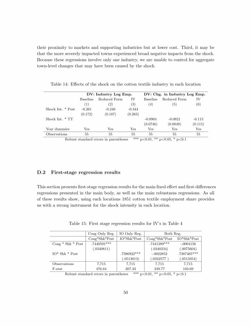
their proximity to markets and supporting industries but at lower cost. Third, it may bethat the more severely impacted towns experienced broad negative impacts from the shock.Because these regressions involve only one industry, we are unable to control for aggregatetown-level changes that may have been caused by the shock.
Table 14: Effects of the shock on the cotton textile industry in each location
DV: Industry Log Emp. DV: Chg. in Industry Log Emp.
Baseline Reduced Form IV Baseline Reduced Form IV
(1) (2) (3) (4) (5) (6)
Shock Int. * Post -0.261 -0.246 -0.344
(0.172) (0.187) (0.263)
Shock Int. * TT -0.0904 -0.0821 -0.115
(0.0746) (0.0849) (0.115)
Year dummies Yes Yes Yes Yes Yes Yes
Observations 55 55 55 55 55 55
Robust standard errors in parentheses *** p<0.01, ** p<0.05, * p<0.1
D.2 First-stage regression results
This section presents first-stage regression results for the main fixed effect and first-differencesregressions presented in the main body, as well as the main robustness regressions. As allof these results show, using each locations 1851 cotton textile employment share providesus with a strong instrument for the shock intensity in each location.
Table 15: First stage regression results for IV’s in Table 4
Coag Only Reg. IO Only Reg. Both Reg.
Coag*Shk*Post IO*Shk*Post Coag*Shk*Post IO*Shk*Post
Coag * Shk * Post .7440591*** .7441289*** -.0004156
(.0340811) (.0340234) (.0075604)
IO* Shk * Post .7386922*** -.0022852 .7387465***
(.0513013) (.0322577 ) (.0513354)
Observations 7,715 7,715 7,715 7,715
F-stat 476.64 207.33 239.77 103.69
Robust standard errors in parentheses *** p<0.01, ** p<0.05, * p<0.1
50
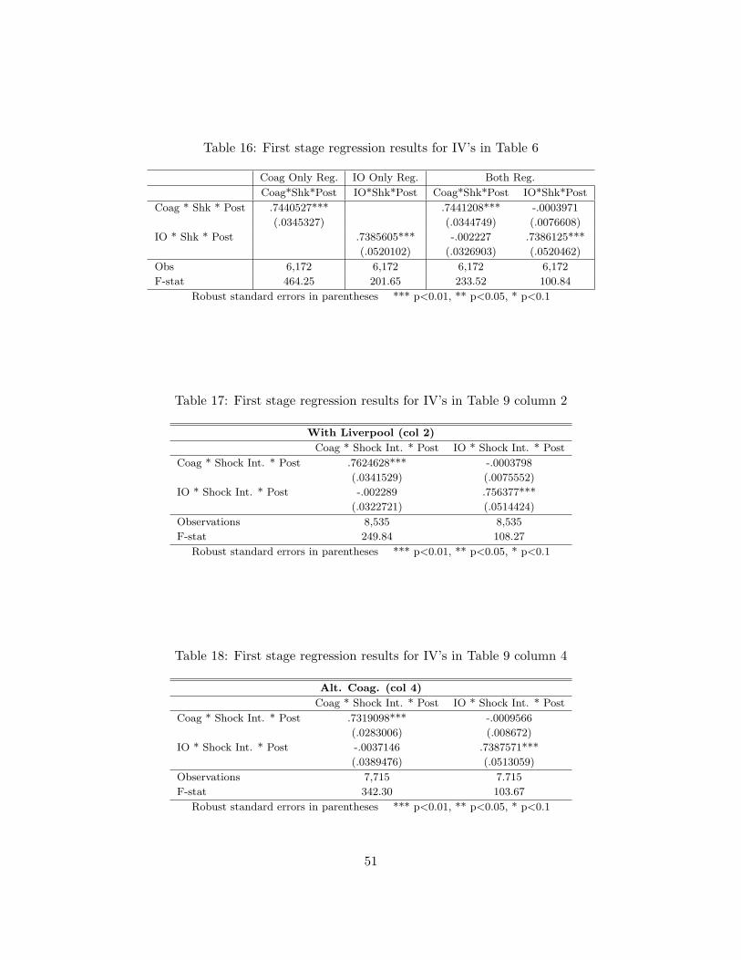
Table 16: First stage regression results for IV’s in Table 6
Coag Only Reg. IO Only Reg. Both Reg.
Coag*Shk*Post IO*Shk*Post Coag*Shk*Post IO*Shk*Post
Coag * Shk * Post .7440527*** .7441208*** -.0003971
(.0345327) (.0344749) (.0076608)
IO * Shk * Post .7385605*** -.002227 .7386125***
(.0520102) (.0326903) (.0520462)
Obs 6,172 6,172 6,172 6,172
F-stat 464.25 201.65 233.52 100.84
Robust standard errors in parentheses *** p<0.01, ** p<0.05, * p<0.1
Table 17: First stage regression results for IV’s in Table 9 column 2
With Liverpool (col 2)
Coag * Shock Int. * Post IO * Shock Int. * Post
Coag * Shock Int. * Post .7624628*** -.0003798
(.0341529) (.0075552)
IO * Shock Int. * Post -.002289 .756377***
(.0322721) (.0514424)
Observations 8,535 8,535
F-stat 249.84 108.27
Robust standard errors in parentheses *** p<0.01, ** p<0.05, * p<0.1
Table 18: First stage regression results for IV’s in Table 9 column 4
Alt. Coag. (col 4)
Coag * Shock Int. * Post IO * Shock Int. * Post
Coag * Shock Int. * Post .7319098*** -.0009566
(.0283006) (.008672)
IO * Shock Int. * Post -.0037146 .7387571***
(.0389476) (.0513059)
Observations 7,715 7.715
F-stat 342.30 103.67
Robust standard errors in parentheses *** p<0.01, ** p<0.05, * p<0.1
51
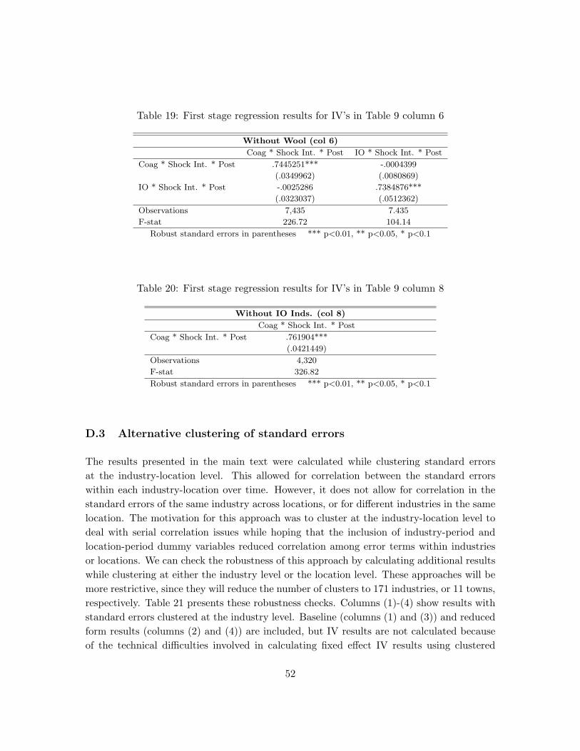
Table 19: First stage regression results for IV’s in Table 9 column 6
Without Wool (col 6)
Coag * Shock Int. * Post IO * Shock Int. * Post
Coag * Shock Int. * Post .7445251*** -.0004399
(.0349962) (.0080869)
IO * Shock Int. * Post -.0025286 .7384876***
(.0323037) (.0512362)
Observations 7,435 7.435
F-stat 226.72 104.14
Robust standard errors in parentheses *** p<0.01, ** p<0.05, * p<0.1
Table 20: First stage regression results for IV’s in Table 9 column 8
Without IO Inds. (col 8)
Coag * Shock Int. * Post
Coag * Shock Int. * Post .761904***
(.0421449)
Observations 4,320
F-stat 326.82
Robust standard errors in parentheses *** p<0.01, ** p<0.05, * p<0.1
D.3 Alternative clustering of standard errors
The results presented in the main text were calculated while clustering standard errorsat the industry-location level. This allowed for correlation between the standard errorswithin each industry-location over time. However, it does not allow for correlation in thestandard errors of the same industry across locations, or for different industries in the samelocation. The motivation for this approach was to cluster at the industry-location level todeal with serial correlation issues while hoping that the inclusion of industry-period andlocation-period dummy variables reduced correlation among error terms within industriesor locations. We can check the robustness of this approach by calculating additional resultswhile clustering at either the industry level or the location level. These approaches will bemore restrictive, since they will reduce the number of clusters to 171 industries, or 11 towns,respectively. Table 21 presents these robustness checks. Columns (1)-(4) show results withstandard errors clustered at the industry level. Baseline (columns (1) and (3)) and reducedform results (columns (2) and (4)) are included, but IV results are not calculated becauseof the technical difficulties involved in calculating fixed effect IV results using clustered
52
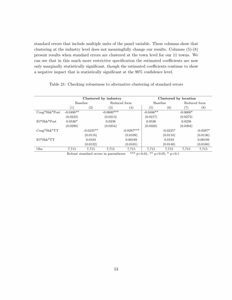
standard errors that include multiple units of the panel variable. These columns show thatclustering at the industry level does not meaningfully change our results. Columns (5)-(8)present results when standard errors are clustered at the town level for our 11 towns. Wecan see that in this much more restrictive specification the estimated coefficients are nowonly marginally statistically significant, though the estimated coefficients continue to showa negative impact that is statistically significant at the 90% confidence level.
Table 21: Checking robustness to alternative clustering of standard errors
Clustered by industry Clustered by location
Baseline Reduced form Baseline Reduced form
(1) (2) (3) (4) (5) (6) (7) (8)
Coag*Shk*Post -0.0486** -0.0600*** -0.0486** -0.0600*
(0.0223) (0.0213) (0.0217) (0.0273)
IO*Shk*Post 0.0536* 0.0238 0.0536 0.0238
(0.0290) (0.0354) (0.0328) (0.0394)
Coag*Shk*TT -0.0235** -0.0287*** -0.0235* -0.0287*
(0.0118) (0.0109) (0.0110) (0.0136)
IO*Shk*TT 0.0183 0.00189 0.0183 0.00189
(0.0132) (0.0165) (0.0140) (0.0160)
Obs 7,715 7,715 7,715 7,715 7,715 7,715 7,715 7,715
Robust standard errors in parentheses *** p<0.01, ** p<0.05, * p<0.1
53