Industry Effect, Credit Contagion and Bankruptcy …centerforpbbefr.rutgers.edu/2012PBFEAM/papers/060-Han-Hsing Lee... · Industry Effect, Credit Contagion and Bankruptcy Prediction

Industry Effect, Credit Contagion and

Bankruptcy Prediction

By

Han-Hsing Lee* Corresponding author: National Chiao Tung University, Graduate Institute of Finance, Taiwan

E-mail: [email protected] Fax: 886-3-573-3260 Phone: 886-3-571-2121 Ext. 57076

Che-Ming Lin National Chiao Tung University, Graduate Institute of Finance, Taiwan

E-mail: [email protected] Phone: 886-3-571-2121

Industry Effect, Credit Contagion and Bankruptcy

Prediction

Abstract

In this paper, we examine the effect of intra-industry credit contagion using three different

kinds of intra-industry measures in our empirical study. We apply the competitive strategic

measure (CSM) of Sundaram et al. (1996) to capture the strategic interaction faced by firms.

We also consider the measure of industry-wide financial distress and the measure of equity

correlations. We use the forward intensity approach proposed by Duan et al. (2010) to

examine if these industry measures can affect default intensity. Our empirical results suggest

that intra-industry contagion effect may be characterized by the level of industry-wide

financial distress or equity correlations among firms.

Keywords: Credit Contagion, Intra-Industry Interaction, Strategic Competition,

Industry-Wide Financial Distress, Bankruptcy Prediction

1. Introduction

The recent global financial crisis has impacted the financial markets around the world,

and raises the importance of the forecast of credit events. Credit contagion has been

considered as a possible major cause of why the corporate defaults cluster in the global

financial crisis. Although it is well-documented in literature that asset returns become more

correlated during financial crisis, debate is still ongoing about the explanation of the

increasing comovement in asset returns – Can the heightened correlation during crisis be

explained by the more correlated fundamentals? Or alternatively, can correlation increase

beyond the explain ability of fundamentals, the condition that Bekaert, Harvey, ang Ng (2005)

refer to as contagion? In prior literature of credit contagion, researchers indicated that industry

characteristics can affect the bankruptcy probabilities and how credit risks propagate.

However, the prevailing reduce-form models rarely consider this important factor. Therefore,

in this study, we attempt to approach this issue by investigating the impact of industry effects

on bankruptcy prediction and credit contagion.

Credit risk modeling can be classified into two categories: structural-form and

reduce-form approaches. Structural-form models, pioneered by Merton (1974), assume that

valuation of any corporate security can be modelled as a contingent claim on the underlying

value of the firm. These models implicitly assume that firm value has contained sufficient

information for the probability of bankruptcy. However, Bharath and Shumway (2008)

indicated that this is unlikely to be the case. Furthermore, recent research in reduced-form

model has greatly improved the accuracy of default forecasting by incorporating

macroeconomic and other firm-specific variables. Therefore, in this study, we perform our

empirical analysis by the reduced-form approach.

The early reduce-form models for bankruptcy prediction employ approaches like

discriminant analysis (Altman 1968) or binary response models such as logit and probit

regresstion (Ohlson 1980; Zmijewski 1984). Shumway (2001) argued that these models

are inconsistent because their single-period static features do not adjust period for risk.

Hazard model proposed by Shumway (2001) can incorporate time-varying covariates that

change with time, and this model is later adopted by Chava and Jarrow (2004), Hillegeist

et al. (2004) and many others. More recently, Duffie et al. (2007) proposed a doubly

stochastic Poisson intensity approach, which is capable of specifying the time-series

dynamics of the explanatory covariates and is able to estimate likelihood of default over

several future time periods.

The doubly-stochastic assumption implies that the exit of one firm has no direct impact

on the likelihood of default of the other firms. The default times are correlated only as their

exit intensities are correlated through covariates. Unlike the prior models, Lando and Nielsen

(2010) consider the direct effect of one firm’s bankruptcy to the remaining firms, and they

suggested using Hawkes process to model this direct impact of propagation of firms’ default

intensities. Nonetheless, their empirical results found no significant contagion effect. In

contrast, Wang (2010) did find evidence of credit contagion and showed that contagion could

be captured by the economic-wide and sector-wide distress measures. In addition, Wang

(2010) also argued that the specification of Lando and Nielsen (2010) may have

multicollinearity problem so that their results of contagion is not significant.

In addition, Duffie et al. (2007) proposed a doubly stochastic Poisson intensity approach to

jointly model default and other types of firm exits such as mergers and acquisitions in which

state variables governing Poisson intensities are assumed to follow a specific time-series

dynamic. However, every single firm-specific state variable, such as distance to default,

requires estimation and the high-dimensional time dynamics of the state variables is

extremely computationally intensive. For the purpose of multiperiod default prediction,

firm-based study can be expensive. More recently, Duan et al. (2010) proposed a

reduced-form approach based on a forward intensity construction which is also capable of

estimating a firm's default probabilities several periods ahead. Similar to Duffie et al. (2007),

their construction takes into account both defaults/bankruptcies and other types of firm exits.

In addition, this method can also estimate forward default probabilities and cumulative default

probabilities for longer than one future period. The advantage of the forward intensity

approach is that it can estimate term structure of default probabilities solely using the known

data at the time of performing prediction, and can circumvent the difficult task of specifying

time dynamics for covariates. The forward intensity approach can be implemented by

maximum pseudo-likelihood estimation. In particular, the pseudo-likelihood function can be

decomposed into independent components, making it less numerically intensive in estimation.

In credit contagion literature, Jorion and Zhang (2007) and Lang and Stultz (1992) have

documented significant intra-industry contagion effect of bankruptcies by event study. Most

of the reduced-form models, however, do not consider the industry effect. Only a few

exceptions like Chava and Jarrow (2004) has incorporated industry effects. Chava and Jarrow

(2004) revealed the importance of including industry effects into hazard rate estimation.

Nonetheless, they merely consider industries as dummy variables and their interaction terms

with accounting variables, which can only demonstrate the industry differences as well as the

importance levels of accounting variables for different industries. If default intensities are

different across industries with otherwise identical firm-specific characteristics, it is then of

interest to introduce industry related variables, in addition to commonly considered

macroeconomic condition and firm-specific characteristics in the reduced-form models.

Therefore, in this study, we attempt to explore the possible credit contagion through the

perspective of intra industry relationship between firms.

In our paper, we focus on the effect of intra-industry interactions on default probabilities,

and use the measures of intra-industry interactions to explain the intra-industry contagion

effect. We estimate the default probability using the forward intensity approach by Duan et al.

(2010), and we consider three different kinds of intra-industry measures in this paper. First,

the Competitive Strategy Measure (CSM) is one of the measures that we use, which is a

measure of strategic competition developed by Sundaram et al. (1996). Sundaram et al. (1996)

argued that profits of individual firm and overall industry profits depend on how firms interact

with each other. Accordingly, firms can increase value by behaving strategically by

committing to actions that will elicit favorable responses from the rivals in the industry. The

definition of strategic competition is that firms face strategic competition when their marginal

profit is influenced by competitors’ action. Therefore, the strategic competition may affect

consequences of financial policies and investment choices. It is of interest to examine whether

the strategic competition can affect the default probabilities of firms. The second measure of

intra-industry interaction is financial distance, since not all the bankruptcy events in an

industry are of equally importance for the remaining survival companies. Financial distance

can be captured by the equity correlation between firms in the same industry. By event study

method, Jorion and Zhang (2007) have shown that equity correlations significantly influence

CDS contagion. Another study by Chen (2010) also modeled the contagion effect by using a

function of equity correlations. The last intra-industry measure is the average of firm's

distance to default in the same industry. Wang (2010) used it to capture the industry-wide

distress, and he argued that the contagion effects are much less significant when he add this

measure to his model. Furthermore, we also include the market-driven variables of Shumway

(2001) and Bharath and Shumway as controls in our empirical analysis. The detail will be

described in section 4.

In Section 2, we briefly review the forward intensity model proposed by Duan (2010). Our

data and variables are described in Section 3. We present our empirical results in Section 4,

and make the conclusion in Section 5.

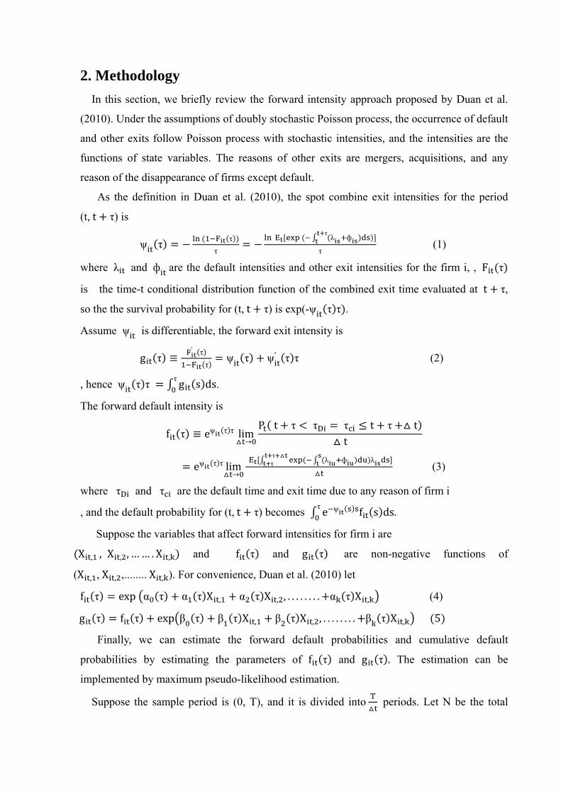
2. Methodology

In this section, we briefly review the forward intensity approach proposed by Duan et al.

(2010). Under the assumptions of doubly stochastic Poisson process, the occurrence of default

and other exits follow Poisson process with stochastic intensities, and the intensities are the

functions of state variables. The reasons of other exits are mergers, acquisitions, and any

reason of the disappearance of firms except default.

As the definition in Duan et al. (2010), the spot combine exit intensities for the period

(t,t τ) is

ψ τ τ

τ

λ фτ

τ (1)

where λ and ф are the default intensities and other exit intensities for the firm i, , F τ

is the time-t conditional distribution function of the combined exit time evaluated at t τ,

so the the survival probability for (t,t τ) is exp(-ψ τ τ .

Assume ψ is differentiable, the forward exit intensity is

g τ ≡′ τ

τψ τ ψ′ τ τ (2)

, hence ψ τ τ g s dsτ

.

The forward default intensity is

f τ ≡ eψ τ τ lim→

P t τ τ τ t τ tt

eψ τ τ lim→

λ фττ λ

(3)

where τ and τ are the default time and exit time due to any reason of firm i

, and the default probability for (t,t τ) becomes e ψ f s dsτ

.

Suppose the variables that affect forward intensities for firm i are

X , , X , , …… . X , and f τ and g τ are non-negative functions of

(X , ,X , ,........X , ). For convenience, Duan et al. (2010) let

f τ exp α τ α τ X , α τ X , , . . . . . . . . α τ X , (4)

g τ f τ exp β τ β τ X , β τ X , , . . . . . . . . β τ X , 5

Finally, we can estimate the forward default probabilities and cumulative default

probabilities by estimating the parameters of f τ and g τ . The estimation can be

implemented by maximum pseudo-likelihood estimation.

Suppose the sample period is (0, T), and it is divided into periods. Let N be the total

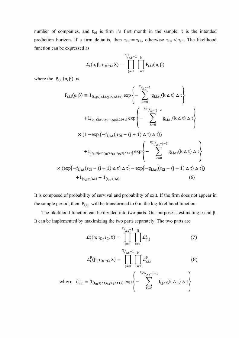
number of companies, and t is firm i’s first month in the sample, τ is the intended

prediction horizon. If a firm defaults, then τ τ , otherwise τ τ . The likelihood

function can be expressed as

τ α, β; τ , τ , X Pτ, , α, β

where the Pτ, , α, β is

Pτ, , α, β ≡ 1 ,τ τ exp g , k t t

1 ,τ τ τ exp g , k t t

τ

1 exp f , τ j 1 t t

1 ,τ τ ,τ τ exp g , k t t

τ

exp f , τ j 1 t t exp g , τ j 1 t t

1 1 τ (6)

It is composed of probability of survival and probability of exit. If the firm does not appear in

the sample period, then Pτ, , will be transformed to 0 in the log-likelihood function.

The likelihood function can be divided into two parts. Our purpose is estimating α and β.

It can be implemented by maximizing the two parts separately. The two parts are

τα α; τ , τ , X τ, ,

α 7

τβ β; τ , τ , X τ, ,

β 8

where τ, ,α 1 ,τ τ exp f , k t t

τ

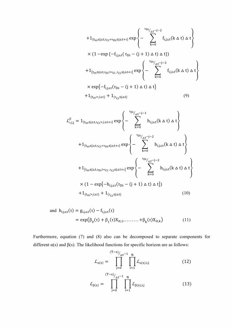
1 ,τ τ τ exp f , k t t

τ

1 exp f , τ j 1 t t

1 ,τ τ ,τ τ exp f , k t t

τ

exp f , τ j 1 t t

1 1 τ (9)

τ, ,β 1 ,τ τ exp h , k t t

τ

1 ,τ τ τ exp h , k t t

τ

1 ,τ τ ,τ τ exp h , k t t

τ

1 exp h , τ j 1 t t

1 1 τ (10)

and h , τ g , τ f , τ

exp β τ β τ X , , . . . . . . . . β τ X , (11)

Furthermore, equation (7) and (8) also can be decomposed to separate components for

different α(s) and β(s). The likelihood functions for specific horizon are as follows:

α α , , 12

β β , , 13

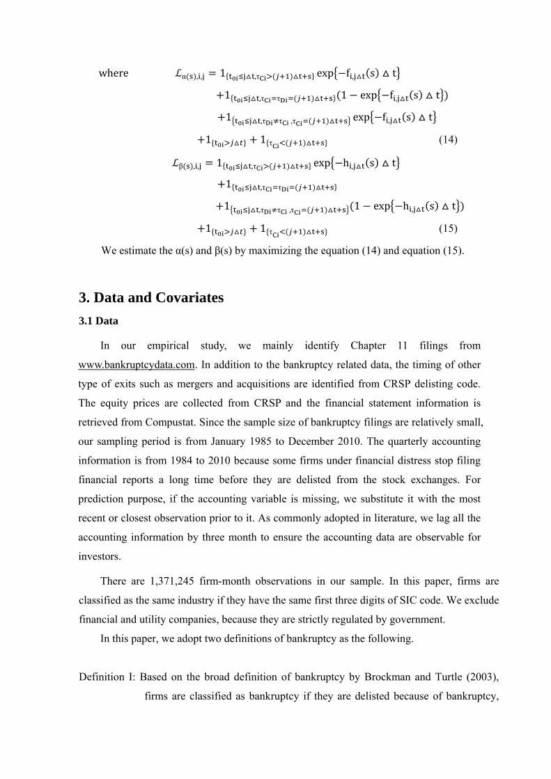
where α , , 1 ,τ exp f , s t

1 ,τ τ 1 exp f , s t

1 ,τ τ ,τ exp f , s t

1 1 τ (14)

β , , 1 ,τ exp h , s t

1 ,τ τ

1 ,τ τ ,τ 1 exp h , s t

1 1 τ (15)

We estimate the α(s) and β(s) by maximizing the equation (14) and equation (15).

3. Data and Covariates

3.1 Data

In our empirical study, we mainly identify Chapter 11 filings from

www.bankruptcydata.com. In addition to the bankruptcy related data, the timing of other

type of exits such as mergers and acquisitions are identified from CRSP delisting code.

The equity prices are collected from CRSP and the financial statement information is

retrieved from Compustat. Since the sample size of bankruptcy filings are relatively small,

our sampling period is from January 1985 to December 2010. The quarterly accounting

information is from 1984 to 2010 because some firms under financial distress stop filing

financial reports a long time before they are delisted from the stock exchanges. For

prediction purpose, if the accounting variable is missing, we substitute it with the most

recent or closest observation prior to it. As commonly adopted in literature, we lag all the

accounting information by three month to ensure the accounting data are observable for

investors.

There are 1,371,245 firm-month observations in our sample. In this paper, firms are

classified as the same industry if they have the same first three digits of SIC code. We exclude

financial and utility companies, because they are strictly regulated by government.

In this paper, we adopt two definitions of bankruptcy as the following.

Definition I: Based on the broad definition of bankruptcy by Brockman and Turtle (2003),

firms are classified as bankruptcy if they are delisted because of bankruptcy,

liquidation or poor performance. Specifically, a firm is considered as broad

definition of bankruptcy if it is given a CRSP delisting code of 400 to 499, or

550 to 599. Under this definition, there are 5,093 defaulted firms in our sample.

Definition II: Firms that file Chapter 11 or firms with CRSP delisting code between 400 and

490. Under the definition II, the total number of bankruptcy firms is 1,276.

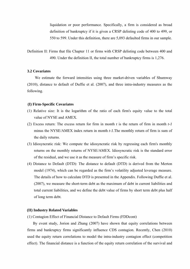
3.2 Covariates

We estimate the forward intensities using three market-driven variables of Shumway

(2010), distance to default of Duffie et al. (2007), and three intra-industry measures as the

following.

(I) Firm-Specific Covariates

(1) Relative size: It is the logarithm of the ratio of each firm's equity value to the total

value of NYSE and AMEX.

(2) Excess return: The excess return for firm in month t is the return of firm in month t-1

minus the NYSE/AMEX index return in month t-1.The monthly return of firm is sum of

the daily returns.

(3) Idiosyncratic risk: We compute the idiosyncratic risk by regressing each firm's monthly

returns on the monthly returns of NYSE/AMEX. Idiosyncratic risk is the standard error

of the residual, and we use it as the measure of firm’s specific risk.

(4) Distance to Default (DTD): The distance to default (DTD) is derived from the Merton

model (1974), which can be regarded as the firm’s volatility adjusted leverage measure.

The details of how to calculate DTD is presented in the Appendix. Following Duffie et al.

(2007), we measure the short-term debt as the maximum of debt in current liabilities and

total current liabilities, and we define the debt value of firms by short term debt plus half

of long term debt.

(II) Industry Related Variables

(1) Contagion Effect of Financial Distance to Default Firms (FDDcont)

By event study, Jorion and Zhang (2007) have shown that equity correlations between

firms and bankruptcy firms significantly influence CDS contagion. Recently, Chen (2010)

used the equity return correlations to model the intra-industry contagion effect (competition

effect). The financial distance is a function of the equity return correlation of the survival and

defaulted firms. In spirit of Chen (2010), we construct a variable considering the effect of

firms that defaulted during the past 12 months. Let t denote the elapsed time since firm j

defaulted. Corr , , denotes the equity return correlation between firm i and defaulted firm j,

given that firm i and firm j belong to the same industry. Corr , , is calculated by the daily

stock returns during the past 12 months. We specify a time-weighted function of equity

correlation as follows.

The aggregate financial distance to defaulted firms (AFDD) for firm i is

AFDD W Corr , , 17

where W t 12, 11, …… . . , 1,0

To construct this intra-industry contagion variable, we also incorporate the size of

bankruptcy firms. Intuitively, the impact of bankruptcy of larger firm shall be bigger than that

of small firm. The impact shall decrease when time pass by. Accordingly, we define the

FDDcont as each firm’s AFDD times the relative size of bankruptcy firms. The FDDcont can

be expressed as

FDDcont AFDD log W sumofdefaulted irms′valueintheindustry

sumofall irms′valueintheindustry18

where tistheelaspedtimesince irmsdefalut and W .

(2) Contagion Effect of Competitive Strategy Measure (CSM)

We use the competitive strategy measure (CSM) to capture the strategic interactions faced

by firms, which was developed by Sundaram et al (1996). Strategic competition can be

classified as strategic complement and strategic substitute. The firm faces strategic

complement when its marginal profit increases with an increase in the rival's output. If the

firm's marginal profit decreases with an increase in the rival's output, the firm is classified as

strategic substitute. Following Sundaram et al. (1996), the rival is defined as all other firms in

the given industry. The CSM is the correlation of firm’s marginal profit and the change in the

rival’s output. The proxy of marginal profit is the ratio of change in net income to the change

in sales. The rival’s output is defined as the sum of all competitors’ sales. The CSM for firm i

can be expressed as

CSM corr ∆

∆, ∆sales (16)

If the CSM is less than -0.05, firm i is classified as strategic substitute; If the CSM is

greater than 0.05, firm i is classified as strategic complement.

In order to keep as many bankruptcy samples as possible, we modify some conditions of

computing CSM. First, Sundaram et al. (1996) defined the competitors as all other firms that

have the same four digits SIC code. Under this definition, many firms do not have any

competitors. Thus, we define the competitors as all other firms that have the same first three

digits of SIC code. Second, Sundaram et al. (1996) used 40 quarters of net income and sales

data to compute CSM, while we relax it to 12 quarters of data since many defaulted firm's

lives are less than 10 years. The 12 quarters of data include the quarters prior to and the

quarter of estimation. If the firms have any missing values within the past three years, we use

the most recent 12 quarters of data within the past five years. We only compute CSM if firms

have data for at least 12 quarters within the past five years.

We next build the intra-industry contagion variable SScont and SCcont. The SS (SC) is a

dummy variable for strategic substitute (strategic complement); it takes 1 when firms is

classified as strategic substitute (strategic complement) and zero otherwise. Note that CSM is

calculated using quarterly data, thus the CSM are the same within three months for each firm.

Similar to FDDcont, the SScont and SCcont also take into account the size of defaulted firms.

SScont SS log W sumofdefaulted irms′valueintheindustry

sumofall irms′valueintheindustry 19

SCcont SC log W sumofdefaulted irms′valueintheindustry

sumofall irms′valueintheindustry 20

where tistheelaspedtimesince irmsdefalut and W .

(3) DTD : It is the arithmetic average of all the companies' DTD in the given

Industry. Wang (2010) measures the industry-wide distress with this variable. To mitigate

collinearity problem, we follow Wang (2010) to replace the DTD with DTD when we

include DTD in the model. DTD is DTD minus DTD .

To eliminate the potential effect of outliers, we follow Shumway (2001) to winsorize the

market-driven variables at 1% and 99% level in our empirical tests. In order to understand

which industry-wide variable has better explanatory power, we construct three models for

different intra-industry measures, each including all the four market-driven variables. Note

that many firms have lives for less than three years. It means we are unable to calculate CSM

of these firms. We exclude these firms when we examine the effect of strategic competition,

and the number of samples of CSM model is less than other two models.

4. Empirical Result

Before we estimate the forward intensities, we divide the sample into the estimation

group and the prediction group. The estimation group contains all the data over the period

1985 to 2007, and the monthly-samples from 2008 to 2010 are classified as prediction group.

We estimate the parameters of forward intensities using only the data in estimation group, and

apply the coefficients obtained to perform the out-of-sample prediction accuracy analyses.

4.1 Parameter Estimates

In this section, we estimate the α(τ) and β(τ) for various τ ranging from 0 to 5 months.

We test three models for different measures of intra-industry effect under two definitions of

bankruptcy. First, we report the correlation matrix of variable in Table 1. The estimated results

are shown in Tables 2 to 7. We focus on how these variables can affect default probabilities,

which are reflected in the estimates of α(τ)s. The reason of the other exits may be too

complicated, thus it is not of interest in this study to examine the significance of β(s).

[INSERT TABLES 1‐4 HERE].

In Table 2, one can find that the FDDcont significantly influences the default intensities.

The default probability is higher when the firm has higher equity return correlation to

bankruptcy firms. The positive coefficients of FDDcont indicate that the financial correlations

affect the default correlations. The significance of FDDcont also suggests that the impacts of

defaults of large firms are bigger than those of small firms, as expected.

On the contrary, in Table 3, there is no significant difference between firms that face

strategic competitions or not. The estimated coefficients of SCcont and SScont are not

statistically significant when τ is greater than two months. It appears that the measure of

strategic competition cannot explain the industry-wide contagion effect. It may be due to the

fact that the sample size is much smaller due to the 12 quarters requirement to compute CSM.

For each quarter, we calculate the CSM when firms have at least 12 quarterly data during the

past 5 years.

In Table 4, we also find that forward default intensities decrease with the increase in

DTD . This is consistent with the findings of Wang (2010). The negative estimated

coefficients of DTD mean that default probabilities of firms increase under the

industry-wide financial distress. The default probabilities are high when all the firms have

high default risk in the industry. That may potentially explain clustered defaults of firms in

the given industry.

For each model, all the four market-driven variables are statistically significant for different

τs, and their signs are consistent to previous literature. Firms that have large size, low

idiosyncratic risk, and high excess return have lower default probabilities. Using forward

intensity approach, our results regarding the significance of market variables are consistent

with Shumway (2001), Bharath and Shumway (2008) and Duffie et al. (2007). More

importantly, our results also indicate that the FDDcont and DTD siginificantly

influence default intensities, and they are useful variables in explaining the industry-wide

contagion effect.

For the estimates of bankruptcy definition II in Tables 5 to 7, most of the results are very

similar to those in Tables 2 to 4 in terms of statistical significance. We also estimated the

parameters of the model that only include market-driven variables. The results are similar to

Tables 2 to 4. To conserve space, we do not present the results. We estimate these coefficients

in order to test whether the predictive performance is better incorporating intra-industry

measures to the existing market-driven variables.


4.2 Out-of-sample Prediction Accuracy

In this section, we report the bankruptcy prediction performance adding intra-industry

measure using the ROC curves and accuracy ratios. We focus the analysis on FDDcont and

DTD due to the lack of significance of CSM. To compare the out-of-sample prediction

performance, one needs to estimate the cumulative default probability before plotting ROC

curves. According to Duan et al. (2010), The cumulative default probability at time t for the

future period (t, t τ) is

P t τ τ t τ

e ψ 1 e

τ

18

We apply the estimated coefficients obtained from estimation group (1985-2007) to

prediction group (2008-2010) to compute the cumulative default probabilities of each

firm-month sample. We report the ROC curves and accuracy ratios for 1-month- and

6-month- ahead bankruptcy prediction, in Figures 1 and 2, respectively. All models in the AR

test include 4 firm-specific market variables. We term the benchmark model Shumway model,

which contains only 4 firm-specific variables; DTD and Financial Distance models

add the industry measures DTD and Financial Distance, respectively.

[INSERT FIGURES 1‐2 HERE].


In Figure 1, comparing the effect of industry variables, DTD model (AR =

0.8627) is the best performing model, followed by Financial Distance model (AR = 0.8579),

and Shumway model with only four firm-specific variables (AR = 0.8261). It is apparent that

considering industry variables can enhance out-of-sample prediction accuracy. The

differences of AR ratios are statistically significant in Table 8. We found that the predictive

performance is substantially enhanced after adding DTD or financial distance to the

Shumway model. Similar results are also obtained from the 6-month prediction analysis in

Figure 2 and Table 9. In sum, the out-of-sample prediction analyses indicate that DTD

and financial distance are useful when one needs to forecast firms’ default probabilities. The

introduction of industry-wide variables do improve the performance of bankruptcy prediction.

5. Conclusion

We use three different kinds of measures to capture the intra-industry contagion effects,

and examine how these measures affect default probabilities. The empirical evidence shows

that a firm's default probability significantly increases when the level of industry-wide distress

is higher. It also appears that the default probability of a firm is higher when the returns of the

firm are more positively related to defaulted firms. The lack of significance of strategic

competition may be due to the limitation when computing CSM since it requires a long

history of accounting data. Nonetheless, it leads to loss of a large proportion of the sample

firms. It is evident that the out-of-sample predictive performance is substantially enhanced

when we add contagion variable of financial distance or DTD into the model. Overall,

our results suggest that intra-industry contagion effect may be characterized by the level of

industry-wide financial distress or the equity correlations among firms.

Reference

Acharya, V.. V., S. T. Bharath, and A. Srinivasan, 2007, Does industry-wide distress affect defaulted firms? Evidence from creditor recoveries, Journal of Financial Economics 85, 787-821.

University Working Paper. Bekaert, G., C. R. Harvey, and A. Ng, 2005, Market Integration and Contagion. The Journal

of Business 78(1), 39–69. Bharath, S. T., and T. Shumway, 2008, Forecasting default with the Merton distance to default model, Review of Financial Studies 21, 1339-1369. Chava, Sudheer, and Robert A. Jarrow, 2004, Bankruptcy prediction with industry effects, Review of Finance 8, 537-569. Das, S. R., D. Duffie, N. Kapadia, and L. Saita, 2007, Common failings: How corporate defaults are correlated, Journal of Finance 62, 93-117. Duan, J. C., 2000, Correction: "Maximum likelihood estimation using price data of the derivative contract", Mathematical Finance 10, 461-462. Duan, J. C., J. Sun and T. Wang, 2010, Multiperiod corporate default prediction - A forward intensity approach, National University of Singapore Working Paper. Duffie, D., L. Saita, and K. Wang, 2007, Multi-period corporate default prediction with stochastic covariates, Journal of Financial Economics 83, 635-665. Hillegeist, S. A., E. K. Keating, D. P. Cram, and K. G. Lundstedt, 2004, Assessing the

probability of bankruptcy, Review of Accounting Studies 9, 5-34. Jorion, P., and G. Y. Zhang, 2007, Good and bad credit contagion: Evidence from credit default swaps, Journal of Financial Economics 84, 860-883. Lando, D., and M. S. Nielsen, 2010, Correlation in corporate defaults: Contagion or conditional independence, Journal of Financial Intermediation 19 (2010) 355–372. Lang, L. and R. Stulz, 1992, “Contagion and Competitive Intra-Industry Effects of

Bankruptcy Announcements,” Journal of Financial Economics 8, 45-60. Merton, Robert C., 1974, On the pricing of corporate debt: The risk structure of interest rates, Journal of Finance 29, 449-470. Ohlson, J. A., 1980, Financial ratios and the probabilistic prediction of bankruptcy, Journal of

Accounting Research 18, 109-131. Shumway, T., 2001, Forecasting bankruptcy more accurately: A simple hazard model, Journal of Business 74, 101-124. Sundaram, A., John, T., John, K., 1996. An empirical analysis of strategic competition and firm values: The case of R&D competition. Journal of Financial Economics 40, 459–486. Wang, T., 2010, Determinants of corporate default: Systematic distress, sectoral distress and credit contagion, National University of Singapore Working Paper. Zmijewski, M. E., 1984, Methodological issues related to the estimation of financial distress

prediction models, Journal of Accounting Research 22, 59–82.

Appendix

Merton (1974) assumes that the total value of a firm follow geometric Brownian motion,

dV μVdt σ VdB. The second assumption is that the firm is financed by equity and single

discount bond maturing in T period. Under these assumptions, the equity value of the firm is a

call option on the firm's asset value. The equity value of the firm can be expressed as

E V N d e DN d σ √T t

where r riskfreerate

D thedebtvalueofthe irm

dσ

σ √

V firm value

N ∙ the cumulative distribution function of standard normal variable

The distance to default is √

, and the firm's bankruptcy probability at time t is N( DTD )

Before calculating the DTD, one needs to measure the debt value and the volatility of total

firm value. We follow Duffie et al (2007) to set the short-term debt as the maximum of debt in

current liabilities and total current liabilities. The debt value is computed as short-term debt

plus one half of the long-term debt and other liabilities.

Following Bharath and Shumway (2008), we obtain V and σ by solve the following

equations through iterated procedure.

σVEN d σ

E VN d e DN d σ √T

Table 1

Panel A. The correlation matrix of Financial Distance model and model

Relative size Excess return Idiosyncratic risk FDcont DTD DTD DTD Relative size Excess return Idiosyncratic risk FDcont DTD DTD

10.17318

-0.41040-0.010450.515750.44942

0.173181

0.211220.000870.328580.31397

-0.410400.21122

1-0.14824-0.43654-0.29285

-0.010450.00087

-0.436541

0.08053-0.02209

0.515750.32858

-0.436540.08053

10.81256

0.449420.31397

-0.29285-0.022090.81256

1

0.18677 0.07669

-0.29206 0.17035 0.45216

-0.15248 DTD 0.18677 0.07669 -0.29206 0.17035 0.45216 -0.15248 1

Panel B. The correlation matrix of CSM model

Relative size Excess return Idiosyncratic risk SScont SCcont DTD Relative size Excess return Idiosyncratic risk SScont SCcont DTD

1 0.13181 -0.39073 -0.01055 -0.02646 0.52624

0.13181 1

0.26639 -0.00401 -0.00689 0.29304

-0.39073 0.26639

1 0.01730 0.02382 -0.45069

-0.01055 -0.00401 0.01730

1 -0.69509 -0.03179

-0.02646 -0.00689 0.02382 -0.69509

1 -0.03835

0.52624 0.29304 -0.45069 -0.03179 -0.03835

1

Table 2

The estimation results of Financial Distance model (Bankruptcy Definition I)

Maximum likelihood estimations for α(s) of the model

τ 0 1 2 3 4 5 Relative size Excess return Idiosyncratic risk DTD FDcont

-0.876*** (0.01962)

-0.7029*** (0.03193)

4.00908*** (0.14057)

-0.2739*** (0.023)

0.01461*** (0.0049)

-0.8101***(0.0189)

-0.7199***(0.03168)

4.2875***(0.13975)

-0.2655***(0.02195)

0.01783***(0.00506)

-0.7347***(0.01766)

-0.7199***(0.03127)

4.28482***(0.13995)

-0.2533***(0.02055)

0.01595***(0.00487)

-0.6829***(0.01706)

-0.7251***(0.031)

4.22043***(0.14132)

-0.2321***(0.01974)

0.01791***(0.00507)

-0.6376*** (0.01621)

-0.7165*** (0.03029)

4.13234*** (0.14056)

-0.2262*** (0.01827)

0.01702*** (0.00506)

-0.6007***(0.01565)

-0.6729***(0.03015)

4.07414***(0.1418)

-0.2153***(0.01729)

0.02037***(0.00533)

Maximum likelihood estimations for β(s) of the model

Τ 0 1 2 3 4 5 Relative size Excess return Idiosyncratic risk DTD FDcont

-0.0072 (0.0083)

0.75509*** (0.02826)

-0.6665*** (0.1754)

0.02295*** (0.00531)

-0.0324*** (0.00422)

0.01403*(0.00828)

0.67175***(0.02795)

-0.0098(0.17044)

0.01456***(0.00536)

-0.0289***(0.00413)

0.02253***(0.0082)

0.549***(0.0283)0.11266

(0.17083)-0.0036

(0.00549)-0.0269***

(0.00419)

0.01742**(0.00814)

0.40602***(0.02841)

-0.1368(0.17361)

-0.0186***(0.00564)

-0.0271***(0.00402)

0.01249 (0.0081)

0.25376*** (0.02917) -0.386**

(0.18114) -0.0295***

(0.00581) -0.0263***

(0.00407)

0.00984(0.00805)

0.16325***(0.02918)

-0.7341***(0.18626)

-0.0414***(0.00593)

-0.0269***(0.00404)

One, two and three asterisks (*) represent significance at the 1%, 5% and 10% level; the number in brackets are standard errors of estimated coefficients.

Table 3

The estimation results of CSM model (Bankruptcy Definition I)


τ 0 1 2 3 4 5 Relative size Excess return Idiosyncratic risk DTD SCcont SScont

-0.9243*** (0.035269) -0.542*** (0.072069) 1.86517*** (0.378954) -0.2477*** (0.03724) 0.02312*** (0.00772) 0.02581*** (0.007666)

-0.9178***(0.036724)-0.5666***(0.073248)2.31113***(0.381823)-0.2403***(0.038681)-0.0025 (0.008821)-0.0015 (0.008842)

-0.7694***(0.032836)-0.8754***(0.06863) 5.07013***(0.3128) -0.1938***(0.034826)0.00799 (0.008177)0.00792 (0.008145)

-0.7493***(0.031113)-0.5749***(0.0687) 2.07944***(0.350587)-0.315*** (0.033802)0.01031 (0.00824) 0.00863 (0.007999)

-0.7196*** (0.029504) -0.5704*** (0.065228) 2.18216*** (0.340281) -0.312*** (0.032252) 0.00323 (0.007963) 0.00116 (0.007715)

-0.616*** (0.027046)-0.7211***(0.060712)4.70787***(0.288818)-0.2445***(0.029489)0.01104 (0.007661)0.00472 (0.007398)



-0.0368*** (0.011171) 0.88752*** (0.037279) -0.0128 (0.267312) 0.06603*** (0.007408) -0.0029 (0.005081) 0.00271 (0.005092)

-0.0242** (0.011144)0.84481***(0.038129)0.19122 (0.271273)0.05307***(0.007387)-0.0068 (0.005145)0.0002 (0.005182)

-0.0183* (0.010979)0.70618***(0.039514)0.24274 (0.272525)0.03593***(0.007535)-0.0093* (0.005176)-0.0008 (0.005238)

-0.0197* (0.010884)0.54853***(0.039543)0.09131 (0.264007)0.02484***(0.007586)-0.0106** (0.005192)-0.002 (0.005292)

-0.0212** (0.010717) 0.32094*** (0.041665) 0.00526 (0.269693) 0.01206 (0.007687) -0.0158*** (0.005267) -0.0068 (0.005362)

-0.0234** (0.010711)0.17644***(0.041835)-0.1102 (0.272187)0.0018 (0.007798)-0.0134** (0.005241)-0.0038 (0.005337)


Table 4

The estimation results of model (Bankruptcy Definition I) Maximum likelihood estimations for α(s) of the model

τ 0 1 2 3 4 5 Relative size Excess return Idiosyncratic risk DTD DTD

-0.8768*** (0.01964)

-0.6909*** (0.03195)

3.96797*** (0.13944)

-0.2363*** (0.02295)

-0.2905*** (0.02409)

-0.8134***(0.01894)

-0.7077***(0.03168)

4.22713***(0.13846)

-0.2347***(0.02199)

-0.2778***(0.02297)

-0.7382***(0.01767)

-0.7091***(0.031250

4.22423***(0.13864)

-0.2305***(0.02076)

-0.2617***(0.02149)

-0.6876***(0.01707)

-0.7138***(0.03096)4.148***(0.13999)

-0.2136***(0.02002)-0.238***(0.02069)

-0.6432*** (0.01618)

-0.7063*** (0.03028)

4.05656*** (0.13933)

-0.2158*** (0.01892)

-0.2283*** (0.01908)

-0.6075***(0.01561)

-0.6613***(0.03007)

3.98216***(0.14061)

-0.2079***(0.01821)

-0.2156***(0.01803)



-0.0046 (0.00816)

0.74395*** (0.0284)

-0.5553*** (0.17566) -0.0173*

(0.00975) 0.03278***

(0.0057)

0.0171(0.00815)

0.66169***(0.02812)

0.09788(0.17066)

-0.0136(0.00965)

0.02101***(0.00579)

0.02683***(0.00811)

0.53992***(0.02853)

0.23064(0.17139)

-0.0157(0.00961)

-0.002(0.00594)

0.02285***(0.00809)

0.39678***(0.02868)

0.00181(0.17415)-0.0214**(0.00966)-0.02***

(0.00609)

0.01871** (0.00808)

0.24455*** (0.02946)

-0.2315 (0.18114)

-0.0233 (0.00964**) -0.0337***

(0.0063)

0.01667**(0.00804)

0.15405***(0.02944)

-0.5614***(0.18574)

-0.0313***(0.00967)

-0.0471***(0.00643)


Table 5

The estimation results of Financial Distance model (Bankruptcy Definition II)


τ 0 1 2 3 4 5 Relative size Excess return Idiosyncratic risk DTD FD

-0.1978*** 0.040746

-0.9097*** 0.120917

4.45584*** 0.464596

-0.7417*** 0.085607

0.15775*** 0.041994

-0.1246***0.388322

-0.8228***0.095639

3.99154***0.391858

-0.8149***0.063824

0.17595***0.030952

-0.0844***0.02573

-0.6696***0.082983

3.52081***0.353904

-0.7995***0.049516

0.12925***0.032281

-0.0816***0.023823

-0.7181***0.079663

3.26598***0.344652

-0.748***0.047429

0.1035***0.030481

-0.0613*** 0.022154

-0.7295*** 0.073838

3.22369*** 0.319277

-0.7008*** 0.04107

0.06432** 0.026802

-0.0427***0.020667

-0.5998**0.070753

3.19576***0.312125

-0.6819***0.036034

0.03549***0.02362


τ 0 1 2 3 4 5 Relative size Excess return Idiosyncratic risk DTD FD

-0.1417*** 0.007442

0.25666*** 0.023697

2.59985*** 0.130328

0.03875*** 0.004513

-0.0096 0.010251

-0.132***0.007455

0.18339***0.023299

3.10881***0.126192

0.03488***0.0045160.00249

0.010107

-0.1346***0.007363

0.0615***0.023002

3.18727***0.122764

0.02119***0.0045880.00723

0.009986

-0.1417***0.007278

-0.0598***0.022799

2.96497***0.121656

0.009*0.0046210.00422

0.009253

-0.1476*** 0.007192

-0.1783*** 0.022738

2.74286*** 0.123333 0.00065

0.004708 0.00642

0.009452

-0.1533***0.007138

-0.2396***0.0225442.462***0.125449

-0.009*0.0047720.00296

0.009519


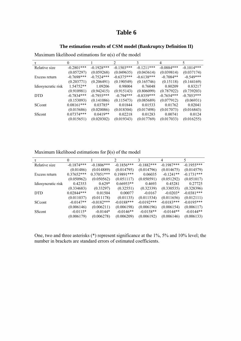
Table 6

The estimation results of CSM model (Bankruptcy Definition II)



-0.2801*** (0.057297) -0.7698*** (0.203771) 1.54752** (0.910981) -0.7834*** (0.153093)

0.08161*** (0.015686)

0.07374*** (0.015651)

-0.1928***(0.059268)-0.7524***(0.206491)

1.09206(0.942415)-0.7955***(0.141086)

0.03785*(0.020086)

0.0419**(0.020302)

-0.1503***(0.049635)-0.6375***(0.190549)

0.98004(0.915143)-0.794***

(0.115473)0.01844

(0.018304)0.02218

(0.019343)

-0.1211***(0.043614)-0.6138***(0.165746)

0.76048(0.806099)-0.8359***(0.085689)

0.01533(0.017498)

0.01283(0.017769)

-0.0884*** (0.039814) -0.7084** (0.15118)

0.80209 (0.787922) -0.7654*** (0.077912)

0.01762 (0.017073)

0.00741 (0.017033)

-0.1014***(0.037174)-0.549***

(0.144169)0.83217

(0.739203)-0.7053***

(0.06931)0.02041

(0.016843)0.0124

(0.016255) Maximum likelihood estimations for β(s) of the model


-0.1874*** (0.01486)

0.37652*** (0.050962)

0.42353 (0.334683)

0.02844*** (0.011037) -0.0147**

(0.006146) -0.0115*

(0.006179)

-0.1806***(0.014889)

0.37051***(0.050562)

0.629*(0.33297)

0.01504(0.011178)-0.0182***(0.006211)

-0.0144*(0.006278)

-0.1856***(0.014795)

0.19891***(0.051117)0.66953**(0.32551)

0.00077(0.01135)

-0.0188***(0.006198)-0.0146**

(0.006209)

-0.1882***(0.014796)

0.06035(0.050591)

0.4693(0.32339)

-0.0167(0.011534)-0.0192***(0.006196)-0.0158**

(0.006192)

-0.1987*** (0.014675) -0.1241**

(0.051292) 0.45281

(0.330535) -0.0203*

(0.011656) -0.0183*** (0.006154) -0.0144**

(0.006146)

-0.1955***(0.014579)-0.1731***(0.051017)

0.27725(0.328396)-0.0381***(0.012111)-0.0195***(0.006117)-0.0144**

(0.006133)


Table 7

The estimation results of model (Bankruptcy Definition II) Maximum likelihood estimations for α(s) of the model


-0.2073*** (0.039795) -0.8823*** (0.120331) 4.29239*** (0.455909) -0.6782*** (0.084717) -0.7654*** (0.085877)

-0.1355***(0.029819)-0.7961***(0.095225)3.79162***(0.386644)-0.7556***(0.063431)-0.834*** (0.063885)

-0.0931***(0.025661)-0.6484***(0.082694)3.3436***(0.348209)-0.755*** (0.050686)-0.8122***(0.049416)

-0.0893***(0.023859)-0.7001***(0.079513)3.10337***(0.339883)-0.714*** (0.04895) -0.7574***(0.047664)

-0.0664*** (0.022309) -0.7164*** (0.073848) 3.10927*** (0.316992) -0.6764*** (0.043424) -0.7077*** (0.041393)

-0.0465** (0.02084) -0.5918***(0.070664)3.11487***(0.307778)-0.6716***(0.039496)-0.684*** (0.036351)



-0.1412*** (0.00742)

0.25566*** (0.023657)

2.61204*** (0.12991)

0.03764*** (0.006719) 0.0389*** (0.004869)

-0.1314***(0.007439)

0.18418***(0.023251)

3.11906***(0.125412)

0.04075***(0.006508)

0.03281***(0.004847)

-0.1334***(0.007356)

0.06343***(0.02297)

3.20546***(0.122019)

0.03375***(0.006427)

0.01672***(0.00488)

-0.1398***(0.007272)-0.0576**

(0.022777)2.99887***(0.120762)

0.02619***(0.006355)

0.0026(0.004898)

-0.1457*** (0.007196) -0.1758*** (0.022708)

2.77739*** (0.122105)

0.01885*** (0.006362)

-0.0061 (0.004977)

-0.1509***(0.007147)-0.2373***(0.022504)2.5088***(0.124053)

0.01115*(0.006368)-0.0166***(0.005025)


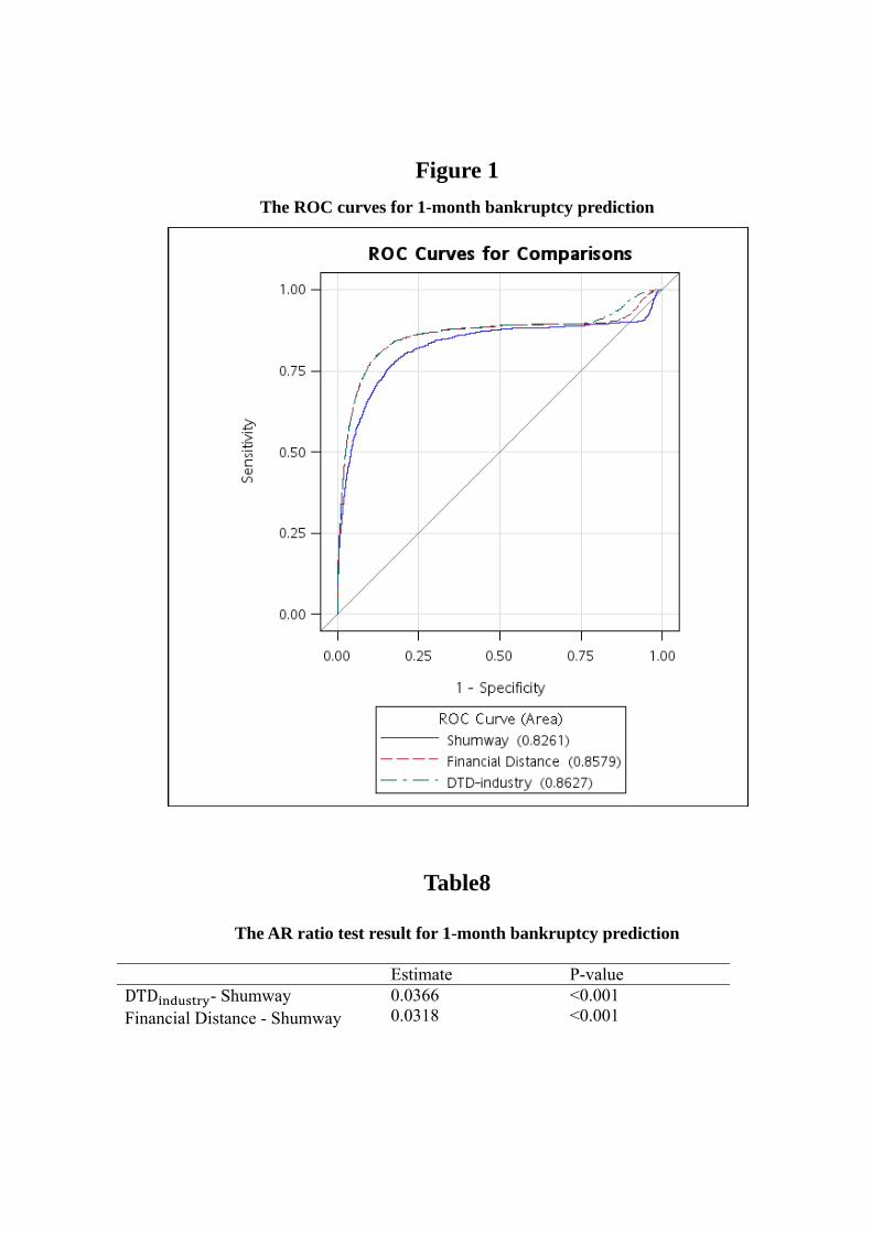
Figure 1

The ROC curves for 1-month bankruptcy prediction

Table8

The AR ratio test result for 1-month bankruptcy prediction

Estimate P-value DTD - Shumway Financial Distance - Shumway

0.0366 0.0318

<0.001 <0.001

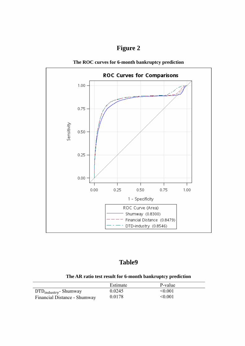
Figure 2

The ROC curves for 6-month bankruptcy prediction

Table9

The AR ratio test result for 6-month bankruptcy prediction

Estimate P-value DTD - Shumway Financial Distance - Shumway

0.0245 0.0178

<0.001 <0.001

Documents

Industry Effect, Credit Contagion and Bankruptcy …centerforpbbefr.rutgers.edu/2012PBFEAM/papers/060-Han-Hsing Lee... · Industry Effect, Credit Contagion and Bankruptcy Prediction