Embed Size (px)
Citation preview
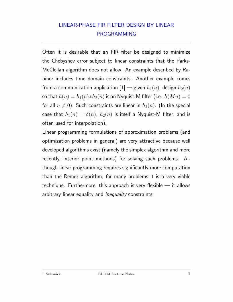
LINEAR-PHASE FIR FILTER DESIGN BY LINEAR
PROGRAMMING
Often it is desirable that an FIR filter be designed to minimize
the Chebyshev error subject to linear constraints that the Parks-
McClellan algorithm does not allow. An example described by Ra-
biner includes time domain constraints. Another example comes
from a communication application [1] — given h1(n), design h2(n)
so that h(n) = h1(n)∗h2(n) is an Nyquist-M filter (i.e. h(Mn) = 0
for all n 6= 0). Such constraints are linear in h2(n). (In the special
case that h1(n) = δ(n), h2(n) is itself a Nyquist-M filter, and is
often used for interpolation).
Linear programming formulations of approximation problems (and
optimization problems in general) are very attractive because well
developed algorithms exist (namely the simplex algorithm and more
recently, interior point methods) for solving such problems. Al-
though linear programming requires significantly more computation
than the Remez algorithm, for many problems it is a very viable
technique. Furthermore, this approach is very flexible — it allows
arbitrary linear equality and inequality constraints.
I. Selesnick EL 713 Lecture Notes 1
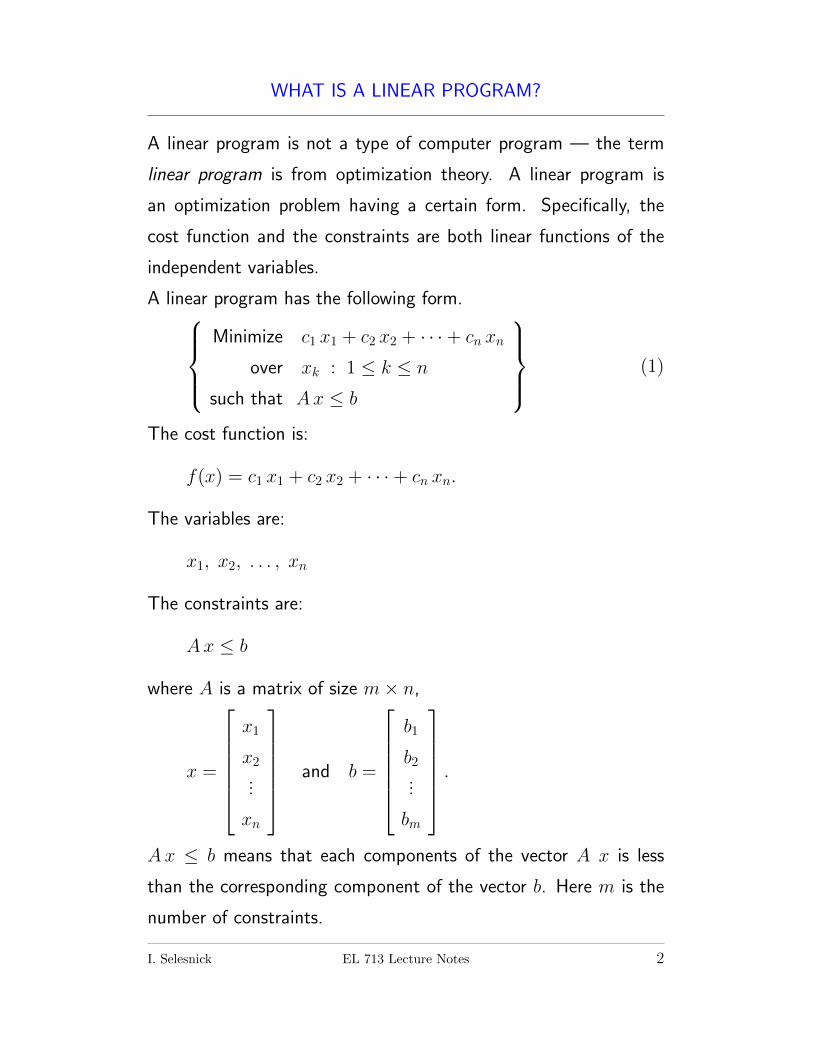
WHAT IS A LINEAR PROGRAM?
A linear program is not a type of computer program — the term
linear program is from optimization theory. A linear program is
an optimization problem having a certain form. Specifically, the
cost function and the constraints are both linear functions of the
independent variables.
A linear program has the following form.Minimize c1 x1 + c2 x2 + · · ·+ cn xn
over xk : 1 ≤ k ≤ n
such that Ax ≤ b
(1)
The cost function is:
f(x) = c1 x1 + c2 x2 + · · ·+ cn xn.
The variables are:
x1, x2, . . . , xn
The constraints are:
Ax ≤ b
where A is a matrix of size m× n,
x =
x1
x2...
xn
and b =
b1
b2...
bm
.A x ≤ b means that each components of the vector A x is less
than the corresponding component of the vector b. Here m is the
number of constraints.
I. Selesnick EL 713 Lecture Notes 2
WHAT IS A LINEAR PROGRAM?
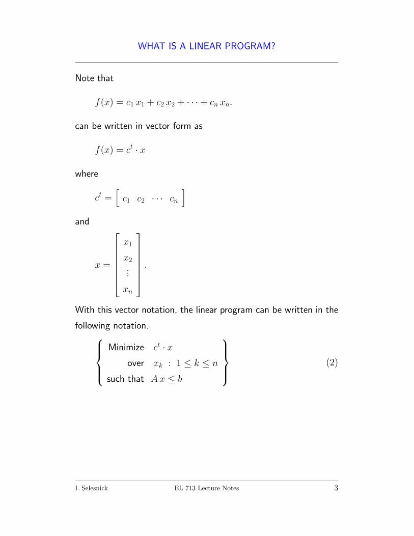
Note that
f(x) = c1 x1 + c2 x2 + · · ·+ cn xn.
can be written in vector form as
f(x) = ct · x
where
ct =[c1 c2 · · · cn
]and
x =
x1
x2...
xn
.With this vector notation, the linear program can be written in the
following notation.Minimize ct · x
over xk : 1 ≤ k ≤ n
such that Ax ≤ b
(2)
I. Selesnick EL 713 Lecture Notes 3
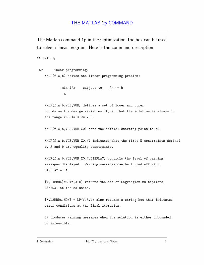
THE MATLAB lp COMMAND
The Matlab command lp in the Optimization Toolbox can be used
to solve a linear program. Here is the command description.
>> help lp
LP Linear programming.
X=LP(f,A,b) solves the linear programming problem:
min f’x subject to: Ax <= b
x
X=LP(f,A,b,VLB,VUB) defines a set of lower and upper
bounds on the design variables, X, so that the solution is always in
the range VLB <= X <= VUB.
X=LP(f,A,b,VLB,VUB,X0) sets the initial starting point to X0.
X=LP(f,A,b,VLB,VUB,X0,N) indicates that the first N constraints defined
by A and b are equality constraints.
X=LP(f,A,b,VLB,VUB,X0,N,DISPLAY) controls the level of warning
messages displayed. Warning messages can be turned off with
DISPLAY = -1.
[x,LAMBDA]=LP(f,A,b) returns the set of Lagrangian multipliers,
LAMBDA, at the solution.
[X,LAMBDA,HOW] = LP(f,A,b) also returns a string how that indicates
error conditions at the final iteration.
LP produces warning messages when the solution is either unbounded
or infeasible.
I. Selesnick EL 713 Lecture Notes 4
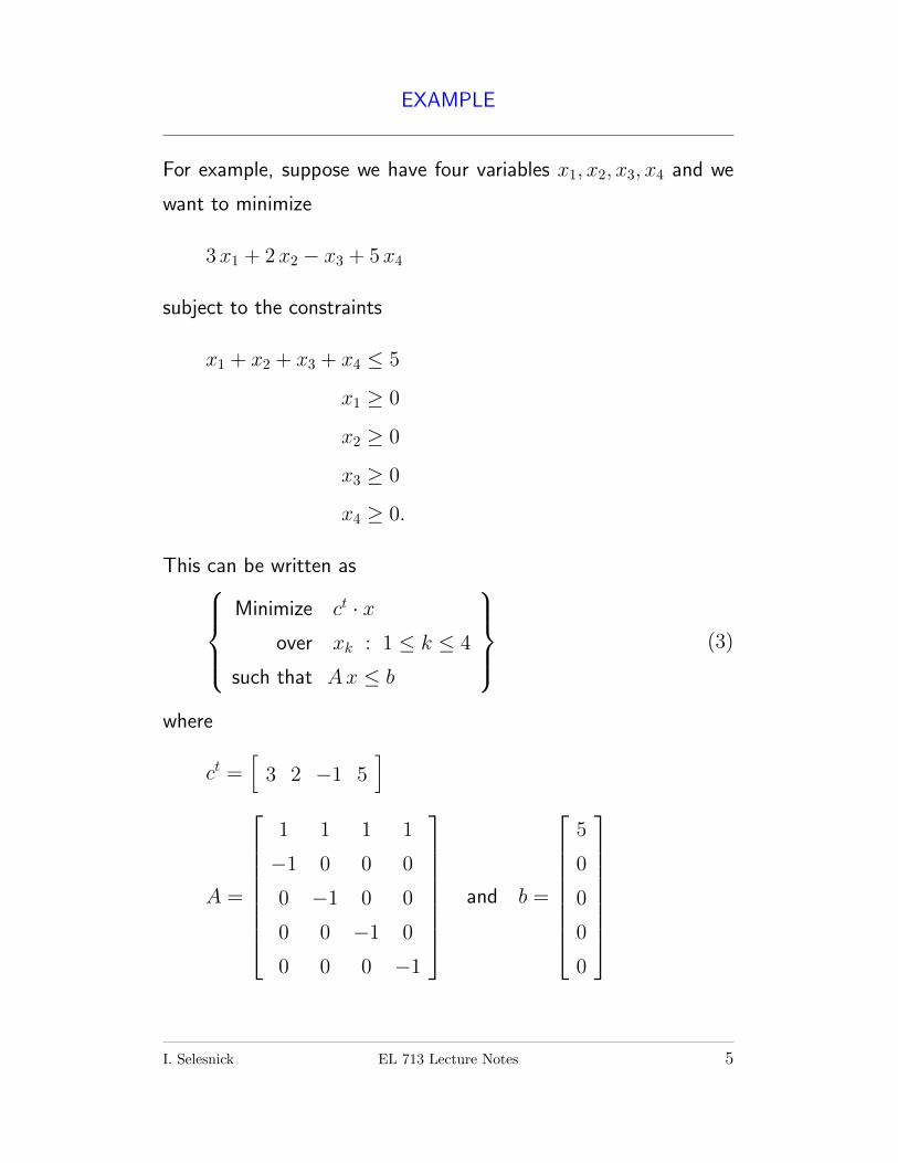
EXAMPLE
For example, suppose we have four variables x1, x2, x3, x4 and we
want to minimize
3x1 + 2x2 − x3 + 5x4
subject to the constraints
x1 + x2 + x3 + x4 ≤ 5
x1 ≥ 0
x2 ≥ 0
x3 ≥ 0
x4 ≥ 0.
This can be written asMinimize ct · x
over xk : 1 ≤ k ≤ 4
such that Ax ≤ b
(3)
where
ct =[3 2 −1 5
]
A =
1 1 1 1
−1 0 0 0
0 −1 0 0
0 0 −1 0
0 0 0 −1
and b =
5
0
0
0
0
I. Selesnick EL 713 Lecture Notes 5
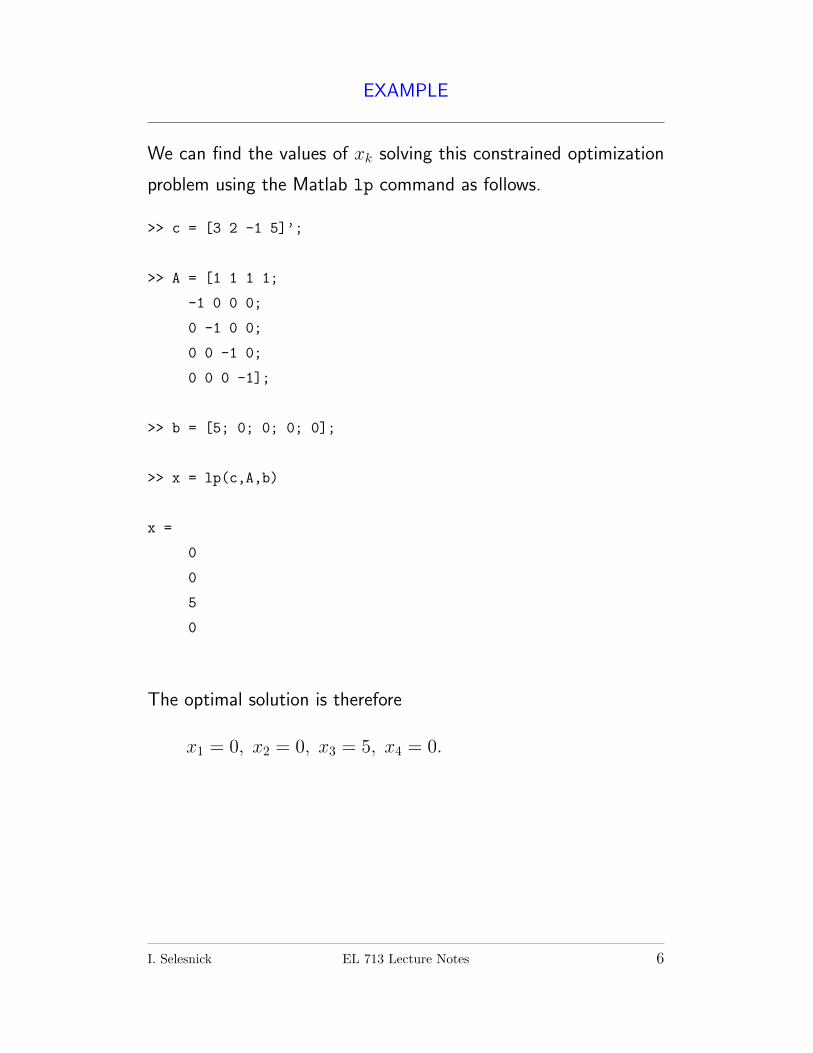
EXAMPLE
We can find the values of xk solving this constrained optimization
problem using the Matlab lp command as follows.
>> c = [3 2 -1 5]’;
>> A = [1 1 1 1;
-1 0 0 0;
0 -1 0 0;
0 0 -1 0;
0 0 0 -1];
>> b = [5; 0; 0; 0; 0];
>> x = lp(c,A,b)
x =
0
0
5
0
The optimal solution is therefore
x1 = 0, x2 = 0, x3 = 5, x4 = 0.
I. Selesnick EL 713 Lecture Notes 6
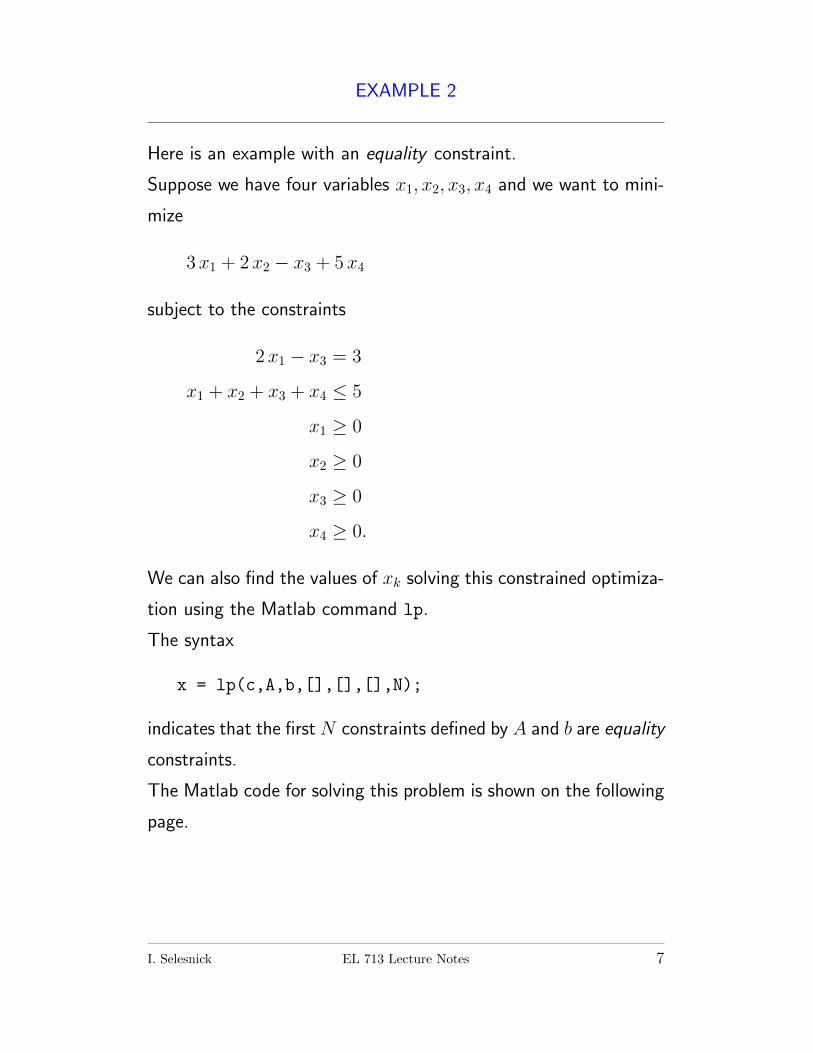
EXAMPLE 2
Here is an example with an equality constraint.
Suppose we have four variables x1, x2, x3, x4 and we want to mini-
mize
3x1 + 2x2 − x3 + 5x4
subject to the constraints
2x1 − x3 = 3
x1 + x2 + x3 + x4 ≤ 5
x1 ≥ 0
x2 ≥ 0
x3 ≥ 0
x4 ≥ 0.
We can also find the values of xk solving this constrained optimiza-
tion using the Matlab command lp.
The syntax
x = lp(c,A,b,[],[],[],N);
indicates that the first N constraints defined by A and b are equality
constraints.
The Matlab code for solving this problem is shown on the following
page.
I. Selesnick EL 713 Lecture Notes 7
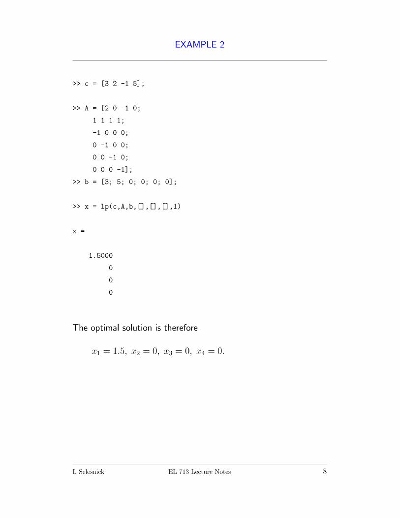
EXAMPLE 2
>> c = [3 2 -1 5];
>> A = [2 0 -1 0;
1 1 1 1;
-1 0 0 0;
0 -1 0 0;
0 0 -1 0;
0 0 0 -1];
>> b = [3; 5; 0; 0; 0; 0];
>> x = lp(c,A,b,[],[],[],1)
x =
1.5000
0
0
0
The optimal solution is therefore
x1 = 1.5, x2 = 0, x3 = 0, x4 = 0.
I. Selesnick EL 713 Lecture Notes 8
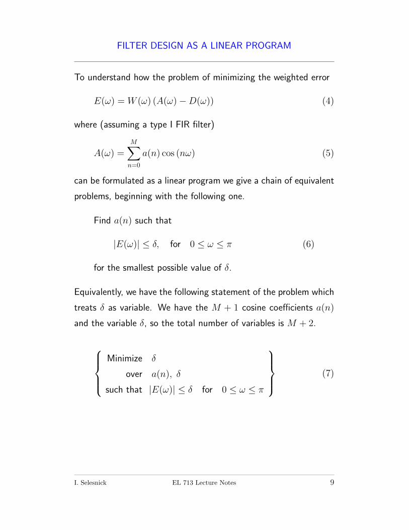
FILTER DESIGN AS A LINEAR PROGRAM
To understand how the problem of minimizing the weighted error
E(ω) = W (ω) (A(ω)−D(ω)) (4)
where (assuming a type I FIR filter)
A(ω) =M∑n=0
a(n) cos (nω) (5)
can be formulated as a linear program we give a chain of equivalent
problems, beginning with the following one.
Find a(n) such that
|E(ω)| ≤ δ, for 0 ≤ ω ≤ π (6)
for the smallest possible value of δ.
Equivalently, we have the following statement of the problem which
treats δ as variable. We have the M + 1 cosine coefficients a(n)
and the variable δ, so the total number of variables is M + 2.
Minimize δ
over a(n), δ
such that |E(ω)| ≤ δ for 0 ≤ ω ≤ π
(7)
I. Selesnick EL 713 Lecture Notes 9
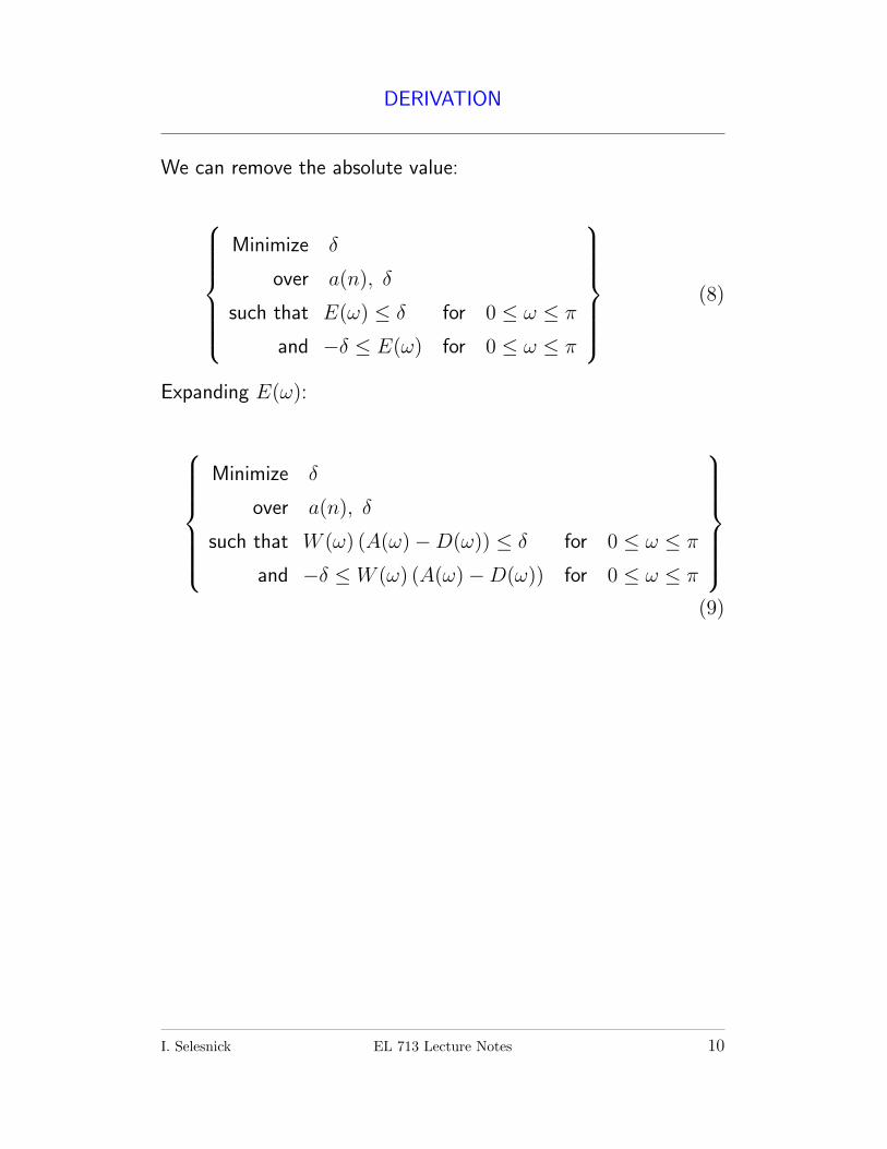
DERIVATION
We can remove the absolute value:
Minimize δ
over a(n), δ
such that E(ω) ≤ δ for 0 ≤ ω ≤ π
and −δ ≤ E(ω) for 0 ≤ ω ≤ π
(8)
Expanding E(ω):
Minimize δ
over a(n), δ
such that W (ω) (A(ω)−D(ω)) ≤ δ for 0 ≤ ω ≤ π
and −δ ≤ W (ω) (A(ω)−D(ω)) for 0 ≤ ω ≤ π
(9)
I. Selesnick EL 713 Lecture Notes 10
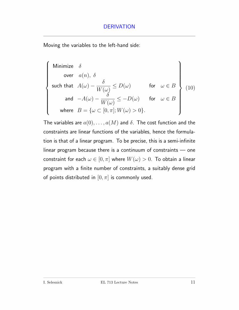
DERIVATION
Moving the variables to the left-hand side:
Minimize δ
over a(n), δ
such that A(ω)− δ
W (ω)≤ D(ω) for ω ∈ B
and −A(ω)− δ
W (ω)≤ −D(ω) for ω ∈ B
where B = {ω ⊂ [0, π];W (ω) > 0}.
(10)
The variables are a(0), . . . , a(M) and δ. The cost function and the
constraints are linear functions of the variables, hence the formula-
tion is that of a linear program. To be precise, this is a semi-infinite
linear program because there is a continuum of constraints — one
constraint for each ω ∈ [0, π] where W (ω) > 0. To obtain a linear
program with a finite number of constraints, a suitably dense grid
of points distributed in [0, π] is commonly used.
I. Selesnick EL 713 Lecture Notes 11
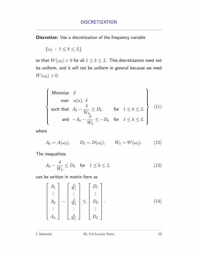
DISCRETIZATION
Discretize: Use a discretization of the frequency variable
{ωk : 1 ≤ k ≤ L}
so that W (ωk) > 0 for all 1 ≤ k ≤ L. This discretization need not
be uniform, and it will not be uniform in general because we need
W (ωk) > 0.
Minimize δ
over a(n), δ
such that Ak −δ
Wk≤ Dk for 1 ≤ k ≤ L
and −Ak −δ
Wk≤ −Dk for 1 ≤ k ≤ L
(11)
where
Ak = A(ωk), Dk = D(ωk), Wk = W (ωk). (12)
The inequalities
Ak −δ
Wk≤ Dk for 1 ≤ k ≤ L (13)
can be written in matrix form as
A1
...
Ak
...
AL
−
δW1
...δWk
...δWL
≤
D1
...
Dk
...
DL
. (14)
I. Selesnick EL 713 Lecture Notes 12
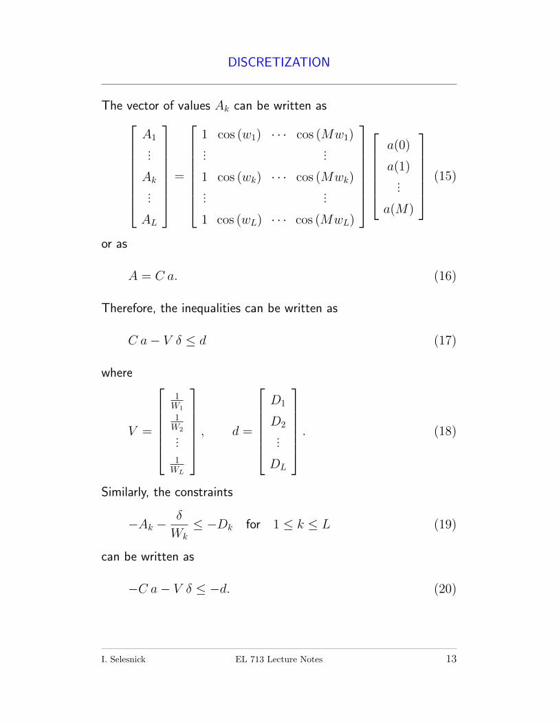
DISCRETIZATION
The vector of values Ak can be written as
A1
...
Ak
...
AL
=
1 cos (w1) · · · cos (Mw1)...
...
1 cos (wk) · · · cos (Mwk)...
...
1 cos (wL) · · · cos (MwL)
a(0)
a(1)...
a(M)
(15)
or as
A = C a. (16)
Therefore, the inequalities can be written as
C a− V δ ≤ d (17)
where
V =
1W1
1W2
...1WL
, d =
D1
D2
...
DL
. (18)
Similarly, the constraints
−Ak −δ
Wk≤ −Dk for 1 ≤ k ≤ L (19)
can be written as
−C a− V δ ≤ −d. (20)
I. Selesnick EL 713 Lecture Notes 13
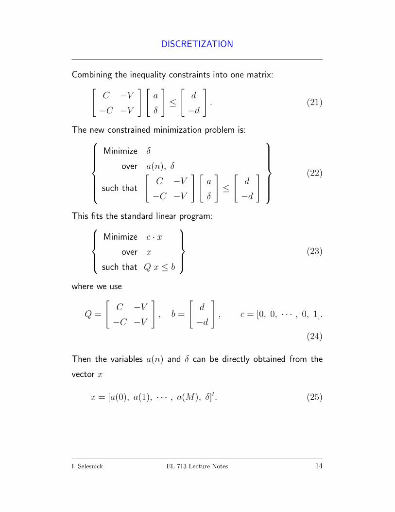
DISCRETIZATION
Combining the inequality constraints into one matrix:[C −V−C −V
][a
δ
]≤
[d
−d
]. (21)
The new constrained minimization problem is:Minimize δ
over a(n), δ
such that
[C −V−C −V
][a
δ
]≤
[d
−d
]
(22)
This fits the standard linear program:Minimize c · x
over x
such that Q x ≤ b
(23)
where we use
Q =
[C −V−C −V
], b =
[d
−d
], c = [0, 0, · · · , 0, 1].
(24)
Then the variables a(n) and δ can be directly obtained from the
vector x
x = [a(0), a(1), · · · , a(M), δ]t. (25)
I. Selesnick EL 713 Lecture Notes 14
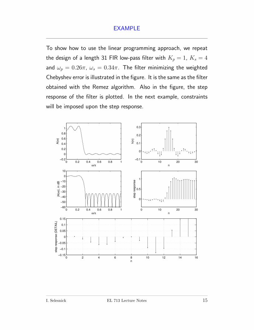
EXAMPLE
To show how to use the linear programming approach, we repeat
the design of a length 31 FIR low-pass filter with Kp = 1, Ks = 4
and ωp = 0.26π, ωs = 0.34π. The filter minimizing the weighted
Chebyshev error is illustrated in the figure. It is the same as the filter
obtained with the Remez algorithm. Also in the figure, the step
response of the filter is plotted. In the next example, constraints
will be imposed upon the step response.
0 0.2 0.4 0.6 0.8 1−0.2
0
0.2
0.4
0.6
0.8
1
ω/π
A(ω
)
0 10 20 30−0.1
0
0.1
0.2
0.3
n
h(n
)
0 0.2 0.4 0.6 0.8 1−60
−50
−40
−30
−20
−10
0
10
ω/π
|A(ω
)|, in
dB
0 10 20 30
0
0.5
1
n
ste
p r
esponse
0 2 4 6 8 10 12 14 16−0.15
−0.1
−0.05
0
0.05
0.1
0.15
n
ste
p r
esponse (
DE
TA
IL)
I. Selesnick EL 713 Lecture Notes 15
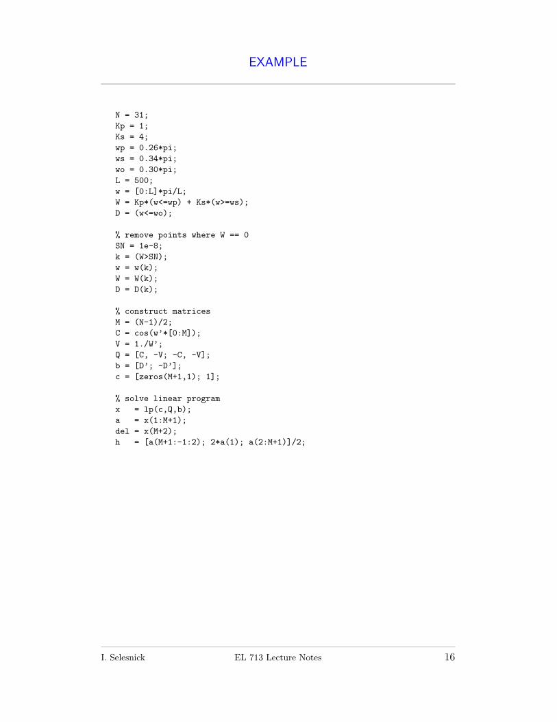
EXAMPLE
N = 31;
Kp = 1;
Ks = 4;
wp = 0.26*pi;
ws = 0.34*pi;
wo = 0.30*pi;
L = 500;
w = [0:L]*pi/L;
W = Kp*(w<=wp) + Ks*(w>=ws);
D = (w<=wo);
% remove points where W == 0
SN = 1e-8;
k = (W>SN);
w = w(k);
W = W(k);
D = D(k);
% construct matrices
M = (N-1)/2;
C = cos(w’*[0:M]);
V = 1./W’;
Q = [C, -V; -C, -V];
b = [D’; -D’];
c = [zeros(M+1,1); 1];
% solve linear program
x = lp(c,Q,b);
a = x(1:M+1);
del = x(M+2);
h = [a(M+1:-1:2); 2*a(1); a(2:M+1)]/2;
I. Selesnick EL 713 Lecture Notes 16
REMARKS
This approach is slower than the Remez algorithm because solving
a linear program is in general a more difficult problem. In this
example, we used a grid density of 500 instead of 1000. Because the
required computation depends on both the number of variables and
the number of constraints, for long filters (which would require more
grid points) the discretization of the constraints may require more
computation than is acceptable. This problem can be alleviated by
a procedure that invokes a sequence of linear programs. By using
a coarse grid density initially, and by appending to the existing set
of constraints, new constraints where the constraint violation is
greatest, a more accurate solution is obtained without the need to
use an overly dense grid.
I. Selesnick EL 713 Lecture Notes 17
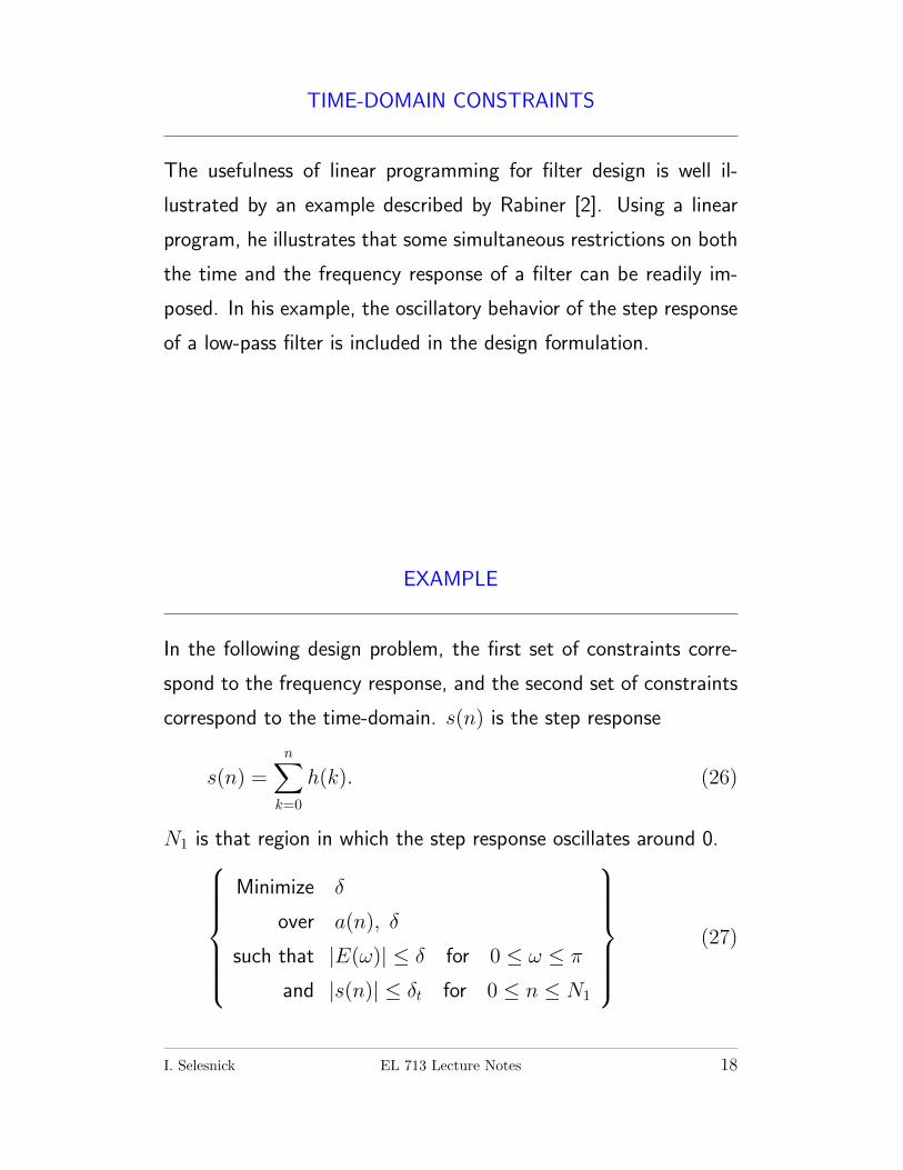
TIME-DOMAIN CONSTRAINTS
The usefulness of linear programming for filter design is well il-
lustrated by an example described by Rabiner [2]. Using a linear
program, he illustrates that some simultaneous restrictions on both
the time and the frequency response of a filter can be readily im-
posed. In his example, the oscillatory behavior of the step response
of a low-pass filter is included in the design formulation.
EXAMPLE
In the following design problem, the first set of constraints corre-
spond to the frequency response, and the second set of constraints
correspond to the time-domain. s(n) is the step response
s(n) =n∑k=0
h(k). (26)
N1 is that region in which the step response oscillates around 0.Minimize δ
over a(n), δ
such that |E(ω)| ≤ δ for 0 ≤ ω ≤ π
and |s(n)| ≤ δt for 0 ≤ n ≤ N1
(27)
I. Selesnick EL 713 Lecture Notes 18
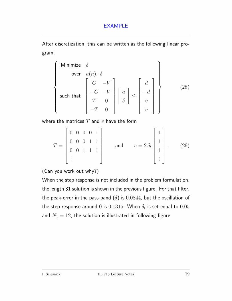
EXAMPLE
After discretization, this can be written as the following linear pro-
gram,
Minimize δ
over a(n), δ
such that
C −V−C −VT 0
−T 0
[a
δ
]≤
d
−dv
v
(28)
where the matrices T and v have the form
T =
0 0 0 0 1
0 0 0 1 1
0 0 1 1 1...
and v = 2 δt
1
1
1...
. (29)
(Can you work out why?)
When the step response is not included in the problem formulation,
the length 31 solution is shown in the previous figure. For that filter,
the peak-error in the pass-band (δ) is 0.0844, but the oscillation of
the step response around 0 is 0.1315. When δt is set equal to 0.05
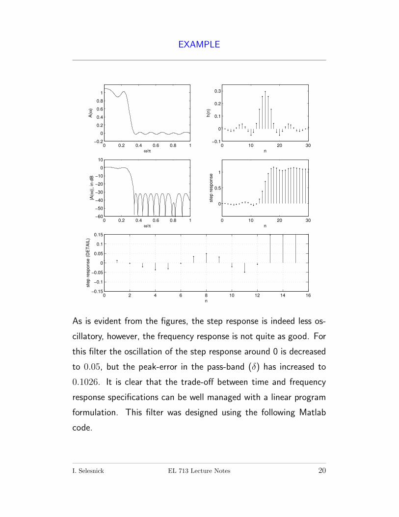
and N1 = 12, the solution is illustrated in following figure.
I. Selesnick EL 713 Lecture Notes 19
EXAMPLE
0 0.2 0.4 0.6 0.8 1−0.2
0
0.2
0.4
0.6
0.8
1
ω/π
A(ω
)
0 10 20 30−0.1
0
0.1
0.2
0.3
n
h(n
)
0 0.2 0.4 0.6 0.8 1−60
−50
−40
−30
−20
−10
0
10
ω/π
|A(ω
)|, in
dB
0 10 20 30
0
0.5
1
n
ste
p r
espo
nse
0 2 4 6 8 10 12 14 16−0.15
−0.1
−0.05
0
0.05
0.1
0.15
n
ste
p r
esponse (
DE
TA
IL)
As is evident from the figures, the step response is indeed less os-
cillatory, however, the frequency response is not quite as good. For
this filter the oscillation of the step response around 0 is decreased
to 0.05, but the peak-error in the pass-band (δ) has increased to
0.1026. It is clear that the trade-off between time and frequency
response specifications can be well managed with a linear program
formulation. This filter was designed using the following Matlab
code.
I. Selesnick EL 713 Lecture Notes 20
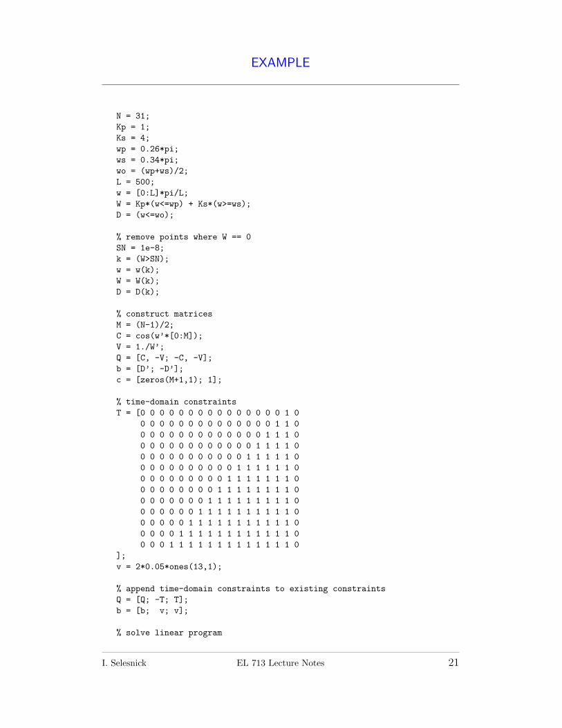
EXAMPLE
N = 31;
Kp = 1;
Ks = 4;
wp = 0.26*pi;
ws = 0.34*pi;
wo = (wp+ws)/2;
L = 500;
w = [0:L]*pi/L;
W = Kp*(w<=wp) + Ks*(w>=ws);
D = (w<=wo);
% remove points where W == 0
SN = 1e-8;
k = (W>SN);
w = w(k);
W = W(k);
D = D(k);
% construct matrices
M = (N-1)/2;
C = cos(w’*[0:M]);
V = 1./W’;
Q = [C, -V; -C, -V];
b = [D’; -D’];
c = [zeros(M+1,1); 1];
% time-domain constraints
T = [0 0 0 0 0 0 0 0 0 0 0 0 0 0 0 1 0
0 0 0 0 0 0 0 0 0 0 0 0 0 0 1 1 0
0 0 0 0 0 0 0 0 0 0 0 0 0 1 1 1 0
0 0 0 0 0 0 0 0 0 0 0 0 1 1 1 1 0
0 0 0 0 0 0 0 0 0 0 0 1 1 1 1 1 0
0 0 0 0 0 0 0 0 0 0 1 1 1 1 1 1 0
0 0 0 0 0 0 0 0 0 1 1 1 1 1 1 1 0
0 0 0 0 0 0 0 0 1 1 1 1 1 1 1 1 0
0 0 0 0 0 0 0 1 1 1 1 1 1 1 1 1 0
0 0 0 0 0 0 1 1 1 1 1 1 1 1 1 1 0
0 0 0 0 0 1 1 1 1 1 1 1 1 1 1 1 0
0 0 0 0 1 1 1 1 1 1 1 1 1 1 1 1 0
0 0 0 1 1 1 1 1 1 1 1 1 1 1 1 1 0
];
v = 2*0.05*ones(13,1);
% append time-domain constraints to existing constraints
Q = [Q; -T; T];
b = [b; v; v];
% solve linear program
I. Selesnick EL 713 Lecture Notes 21
x = lp(c,Q,b);
a = x(1:M+1);
del = x(M+2);
h = [a(M+1:-1:2); 2*a(1); a(2:M+1)]/2;
I. Selesnick EL 713 Lecture Notes 22
REFERENCES REFERENCES
PROS AND CONS
• Optimal with respect to chosen criteria.
• Easy to include arbitrary linear constraints — including in-
equality constraints.
• Criteria limited to linear programming formulation.
• Computational cost higher than Remez algorithm.
References
[1] F. M. de Saint-Martin and Pierre Siohan. Design of optimal linear-
phase transmitter and receiver filters for digital systems. In Proc. IEEE
Int. Symp. Circuits and Systems (ISCAS), volume 2, pages 885–888, April
30-May 3 1995.
[2] L. R. Rabiner and B. Gold. Theory and Application of Digital Signal Pro-
cessing. Prentice Hall, Englewood Cliffs, NJ, 1975.
I. Selesnick EL 713 Lecture Notes 23