Embed Size (px)
Citation preview
Information Geometrical
Study of
Quantum Boltzmann Machines
Nihal Yapage
The University of Electro-Communications
June 2008
Information Geometrical
Study of
Quantum Boltzmann Machines
Nihal Yapage
A thesis submitted to the
Graduate School of Information Systems
The University of Electro-Communications (UEC)
Tokyo, Japan
in partial fulfillment of the requirements for the degree of
Doctor of Philosophy
June 2008
Information Geometrical
Study of
Quantum Boltzmann Machines
Aproved by the supervisory Committee:
Chairperson : Prof. Hiroshi Nagaoka (UEC)
Member : Prof. Masahiro Sowa (UEC)
Member : Prof. Tsutomu Kawabata (UEC)
Member : Prof. Yutaka Sakaguchi (UEC)
Member : Prof. Akio Fujiwara (Osaka University)

Copyright
by
Nihal Yapage
2008
Acknowledgments
First of all, I would like to express my sincere gratitude to my supervisor, Prof.
Hiroshi Nagaoka, for his excellent guidance while working on this work. His extraor-
dinary teaching method was very attractive. The knowledge I retrieved from the
frequent stimulating discussions with him is enormous and undoubtedly led to this
thesis. He taught me not only the subject matter but the logical way of writing a
technical paper also. His inspiring suggestions enhanced the presentation of this the-
sis. On the other hand, my interest to work on such a highly interdisciplinary area
of research was almost fulfilled working with him. I am indebted to him for spending
his time on me despite the heavy work load.
Secondly, I would like to thank Prof. Masahiro Sowa, Prof. Tsutomu Kawabata,
Prof. Yutaka Sakaguchi and Prof. Akio Fujiwara for serving on my thesis committee
and for their valuable suggestions. My thanks also go to all members of the Nagaoka-
Ogawa (formerly Han-Nagaoka) laboratory for their friendship. Since my arrival here
in 2002, the support I received from them (including the former members) in different
ways is gratefully acknowledged. Special thanks are due to Prof. T. S. Han, Dr. T.
Kojima, Dr. T. Ogawa and Dr. M. Iwamoto for participating in my seminars and for
their encouraging comments. Specially, I thank Dr. Ogawa from the bottom of my
heart for his great support in my difficulties.
Thirdly, but most importantly, I must offer my gratitude to my family and others.
I dedicate this thesis to my loving parents for educating me amongst many a hardship.
I am mostly indebted to my loving wife Roshinie and daughter Shanudi for their
love, support, encouragement and endurance, although they were far away from me,
during the past few years. Specially, their support was very important to maintain the
physical and mental stability. It is difficult to find words to express my gratefulness
to my wife for her helping hand extended to me, particularly for taking all the burden
on her shoulders, during the period of my PhD studies. Also I extend my deepest
thanks to all those who supported me throughout my academic career.
Finally, I would like to thank the Ministry of Education, Culture, Sports, Sci-
ence and Technology (Japan) for financial support under the Japanese Government
(Monbukagakusho) Scholarship program.
Nihal Yapage
Graduate School of Information Systems
The University of Electro-Communications
June 2008
i

量子ボルツマンマシンに関する情報幾何学的研究
ヤーパーゲー ニハール
概要
この論文では、確率的ニューラルネットワークの一種として知られているボルツマンマシ
ン(classical Boltzmann machine, 略して CBM)の量子力学系への拡張を考える。具体的に
は、CBM の平衡確率分布の拡張とみなせるような量子状態(密度作用素)を考え、それを
量子ボルツマンマシン (quantum Boltzmann machine, 略して QBM)と呼ぶ。CBM と同様
に、QBM も二種類の実数値パラメータを持つ。すなわち、しきい値(物理的には外場を表
す)h と結合定数 w である。これらのパラメータは、スピングラスの場合のような確率変数
ではなく、任意ではあるが確定した(deterministic な)値を持つものとする。CBM は、単
にニューラルネットワークの一種と言うにとどまらず、統計学的および物理学的な観点から
さまざまな重要な性質を持つ。これらに対応する QBM の性質を明らかにすることがこの研
究の目的である。
CBM の平衡分布の全体は指数型分布族を成す。指数型分布族は統計学および情報幾何学
においてきわめて重要な概念であり、その量子版として量子指数型分布族というものを考え
ると、QBM の全体はその一例になる。また、QBM の全体は滑らかな多様体とみなせ、そこ
に CBM の場合と同様の情報幾何学的構造を導入することができる。これらの数学的枠組み
にもとづいて、まず、与えられた任意の状態を QBM で近似する問題を考察した。近似の規
範として相対エントロピーを用いるとき、CBM の場合と同様の性質および計算アルゴリズ
ムを導いた。ただし、CBM においては近似プロセスを学習問題(パラメータ推定)に適用す
ることができたが、QBM ではそのような直接的応用は見いだせなかった。また、学習と同
様に、CBM の持っていた確率的状態変化則に相当するダイナミクスも、QBM の場合にはそ
の対応物を見いだすことができなかった。ただし、強可分 QBM(strongly separable QBM,
略して SSQBM)という特殊なクラスでは、ギブス・サンプラーの考え方にもとづいて CBM
と同様の状態変化則を導入することができ、幾何学的にも SSQBM の成す多様体と CBM の
成す多様体は同等な構造を持つことを示した。
続いて、QBMに関する平均場近似を情報幾何学的観点から考察した。これらは、T. Tanaka
(田中利幸)によって示されていた CBM に関する結果の量子系への拡張と位置づけられる。
まず、QBM の成す多様体上の情報幾何構造にもとづいて e-射影と m-射影という二種類の射
影概念を定義し、それらを用いてナイーブ平均場近似の幾何学的意味を明らかにするととも
に、その条件を与える平均場方程式を陽に与えた。さらに、統計力学における Plefka 展開の
アイデアによるナイーブ平均場近似の精密化に関して考察を行った。特に、この精密化の本
質を情報幾何学的観点から明らかにするとともに、Plefka 展開の係数が計量や接続などの幾
何学的量によって表されることを示した。
ii
Information Geometrical
Study of
Quantum Boltzmann Machines
Nihal Yapage
Abstract
In this thesis, we consider quantum extension of the well-known stochastic neural
network model called (classical) Boltzmann machine (CBM) from an information
geometrical point of view. The new model is called quantum Boltzmann machine
(QBM). We investigate some properties and geometrical aspects of QBM analogous to
those of CBM. Furthermore, we study the mean-field approximation for such a model
from the information geometrical point of view. This is in some sense motivated by
the application of mean-field approximation for probabilistic inference in the graphical
models in the classical probability theory. Although the problem tackled in the present
thesis is somewhat deviated from the major field of quantum information theory, we
have elucidated the relationships among several well-known fields such as statistical
physics, differential geometry, information theory and statistics using the concepts of
the new emerging subject of quantum information geometry.
We first define QBMs which can be considered as a general class of quantum
Ising spin models. The states we consider are assumed to have at most second-
order interactions with arbitrary but deterministic coupling coefficients. We call such
a state a QBM for the reason that it can be regarded as a quantum extension of
the equilibrium distribution of CBM. The totality of QBMs is then shown to form
a quantum exponential family and thus can be considered as a smooth manifold
having similar geometrical structures to those of CBMs. The information geometrical
structure of the manifold of QBMs is discussed and the problem of approximating a
given quantum state (density operator) by a QBM is also treated.
We also define a restricted class of QBMs called the strongly separable QBMs
(SSQBMs). We consider the dynamics of SSQBMs and propose a new state renewal
rule based on that of CBM. The geometrical structure of the totality of SSQBMs is
shown to be equivalent to that of the totality of CBMs. Approximation process for
SSQBMs is also studied. Finally, we briefly discuss the parameter estimation of a
SSQBM.
Next, we study the mean-field approximation for QBMs from an information geo-
metrical point of view. We elaborate on the significance and usefulness of information
iii

iv
geometrical concepts, in particular the e-(exponential) and m-(mixture) projections,
in studying the naive mean-field approximation for QBMs and derive the naive mean-
field equation explicitly. We also discuss the higher-order corrections to the naive
mean-field approximation based on the idea of Plefka expansion in statistical physics.
We elucidate the geometrical essence of the corrections and provide the expansion
coefficients with expressions in terms of information geometrical quantities. Here,
one may note this work as the information geometrical interpretation of [Ple06] and
as the quantum extension of [Tan00].
Contents
List of Figures vii
List of Symbols viii
1 Introduction 1
1.1 Overview . . . . . . . . . . . . . . . . . . . . . . . . . . . . . . . . . . 1
1.2 Summary of results . . . . . . . . . . . . . . . . . . . . . . . . . . . . 3
1.3 Organization of the thesis . . . . . . . . . . . . . . . . . . . . . . . . 3
2 A review of (classical) Boltzmann machine (CBM) 5
2.1 Definition, state renewal rule and some properties . . . . . . . . . . . 5
2.2 Approximation process and learning . . . . . . . . . . . . . . . . . . . 8
2.3 Mean-field approximation for CBMs . . . . . . . . . . . . . . . . . . . 10
2.3.1 Introduction to mean-field approximation . . . . . . . . . . . . 10
2.3.2 Naive and higher-order mean-field approximations for CBMs . 12
3 A quantum extension of CBM 17
3.1 Definition of quantum Boltzmann machine (QBM) . . . . . . . . . . . 17
3.2 Strongly separable QBM (SSQBM) . . . . . . . . . . . . . . . . . . . 19
3.2.1 Separability criterion and a state renewal rule . . . . . . . . . 19
3.2.2 Strongly separable states and SSQBM . . . . . . . . . . . . . 20
4 Geometry of quantum exponential family and the space of QBMs 25
4.1 Quantum exponential families . . . . . . . . . . . . . . . . . . . . . . 25
4.2 A metric and affine connections . . . . . . . . . . . . . . . . . . . . . 26
4.3 Geometrical structure of the space of QBMs . . . . . . . . . . . . . . 28
4.4 Geometry of quantum relative entropy . . . . . . . . . . . . . . . . . 30
4.5 Approximation processes for QEF and SSQBM . . . . . . . . . . . . 33
v
CONTENTS vi
5 Information geometry of mean-field approximation for QBMs 38
5.1 The e-, m-projections and naive mean-field approximation . . . . . . 38
5.2 Plefka expansion and higher-order mean-field approximations . . . . . 40
5.3 Some possible extensions . . . . . . . . . . . . . . . . . . . . . . . . . 47
6 Concluding remarks 48
6.1 Conclusions . . . . . . . . . . . . . . . . . . . . . . . . . . . . . . . . 48
6.2 Future work . . . . . . . . . . . . . . . . . . . . . . . . . . . . . . . . 49
Bibliography 50
Author Biography 53
List of Publications Related to the Thesis 54
List of Figures
2.1 Approximation process for CBM. . . . . . . . . . . . . . . . . . . . . 9
2.2 Mean-field approximation . . . . . . . . . . . . . . . . . . . . . . . . 11
3.1 State transition process for SSQBM . . . . . . . . . . . . . . . . . . . 24
4.1 Pythagorean theorem D(ρ‖σ) + D(σ‖τ) = D(ρ‖τ) . . . . . . . . . . . 32
4.2 Projection σ from ρ ∈ M to N . . . . . . . . . . . . . . . . . . . . . 33
4.3 Approximation process for QEF. . . . . . . . . . . . . . . . . . . . . . 34
4.4 Approximation process for SSQBM. . . . . . . . . . . . . . . . . . . . 36
5.1 Mutually dual foliations of S2. Here, “e-a.p.” and “m-a.p.” stand for
“e-autoparallel” and “m-autoparallel”, respectively. . . . . . . . . . . 42
5.2 Pythagorean relation D(ρ̂m,0‖ρh,w) = D(ρ̂m,0‖ρ̂m,w) + D(ρ̂m,w‖ρh,w) . 44
vii
List of Symbols and Abbreviations
CBM : classical Boltzmann machine
QBM : quantum Boltzmann machine
SSQBM : strongly separable quantum Boltzmann machine
QEF : quantum exponential family
PVM : projection-valued measure
R : set of real numbers
C : set of complex numbers
ρ, σ, τ : density matrices (operators)
S = S(H) : totality of strictly positive density operators (faithful states)
on a Hilbert space HX1, X2, X3 : Pauli spin matrices (operators)
X∗ : operator adjoint (Hermitian conjugate) of the operator X
I : identity matrix or operator
Tr : trace of a matrix or an operator
M : a family of probability (density) functions
or quantum states (density operators)
|X | : cardinality of a set XP = P(X ) : the set of positive distributions on a set X
‖x‖ : norm of x
D(q‖p) : Kullback-Leibler information divergence of q with respect to p
D(ρ‖σ) : quantum relative entropy of ρ with respect to σ
S(ρ) : von Neumann entropy of ρ
E[x] : expectation of a random variable x
viii
Chapter 1
Introduction
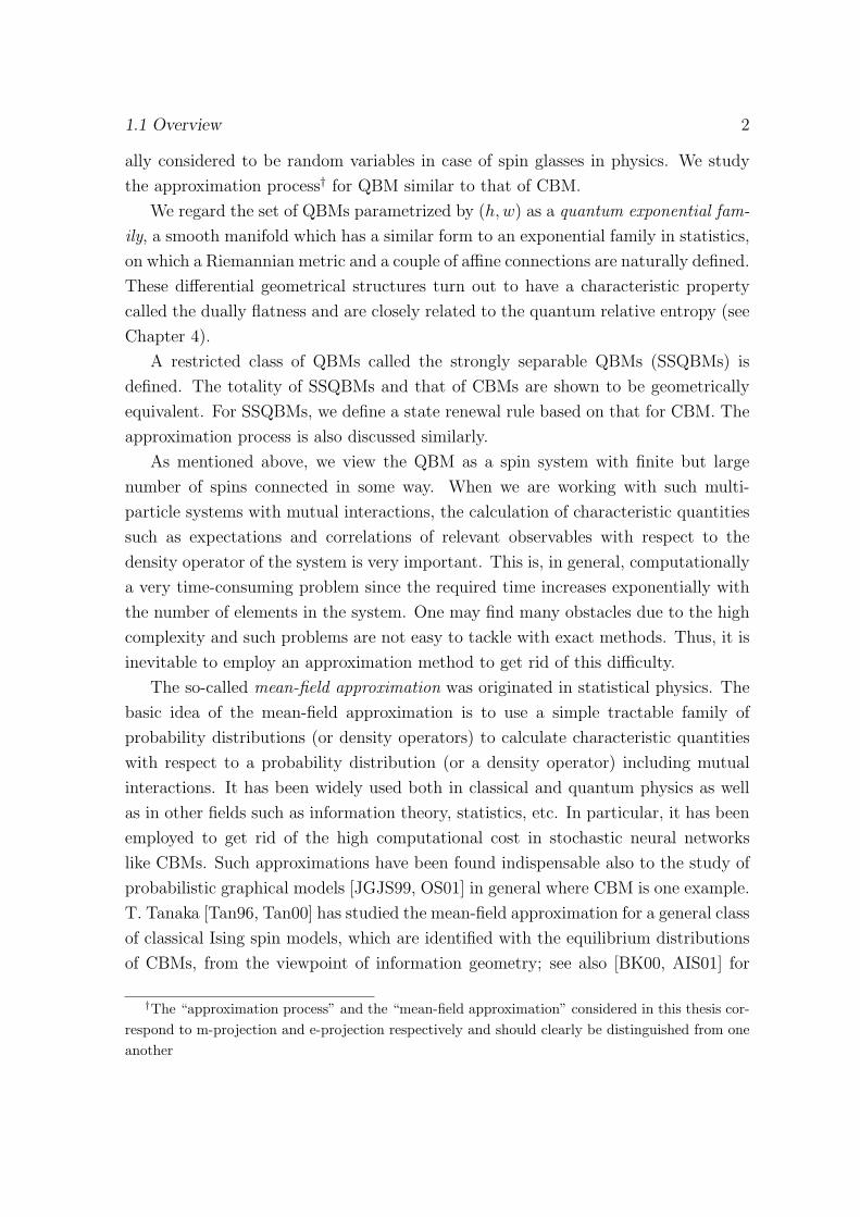
1.1 Overview
It is often both important and interesting to study the problems in the interface
of the fields such as physics, geometry, information theory, and statistics. This paves
the way to the advancement of such fields too. In this thesis, we study a similar
interdisciplinary problem which lies in the interface of such fields.
Information geometry as a new field has been found very useful in understanding
the deep mathematical structures in the interface of many fields [Ama85, AN00]. This
theory has been used in many situations to study the geometrical properties of the
space of parametrized probability distributions or quantum states.
On the other hand, the (classical) Boltzmann machine (CBM) [AHS85] is a well-
known stochastic neural network model. Physically, it can be viewed as a classical
spin system. The statistical aspects of CBM have been elucidated in [NK95]. The in-
formation geometrical structure of the space of CBMs has been discussed in [AKN92].
Stimulated by the above works, we find a possible quantum extension which cor-
respond to the equilibrium distribution of CBM and is called quantum Boltzmann
machine (QBM∗). We can consider QBM as a quantum spin system. Similar to
CBM, each QBM has two kinds of real-valued parameters, namely h, the thresholds
in neural network contexts and the external fields in physical contexts, and w, the
coupling coefficients (to be defined in Section 3.1). We remark that these parameters
are arbitrary but deterministic in our model, while the coupling coefficients are usu-
∗We note that QBM, at present, lacks any notions corresponding to the stochastic dynamics ofCBM which determine its equilibrium distribution. This means that our approach does not suggesthow to quantize the neural aspects of CBM.
1
1.1 Overview 2
ally considered to be random variables in case of spin glasses in physics. We study
the approximation process† for QBM similar to that of CBM.
We regard the set of QBMs parametrized by (h,w) as a quantum exponential fam-
ily, a smooth manifold which has a similar form to an exponential family in statistics,
on which a Riemannian metric and a couple of affine connections are naturally defined.
These differential geometrical structures turn out to have a characteristic property
called the dually flatness and are closely related to the quantum relative entropy (see
Chapter 4).
A restricted class of QBMs called the strongly separable QBMs (SSQBMs) is
defined. The totality of SSQBMs and that of CBMs are shown to be geometrically
equivalent. For SSQBMs, we define a state renewal rule based on that for CBM. The
approximation process is also discussed similarly.
As mentioned above, we view the QBM as a spin system with finite but large
number of spins connected in some way. When we are working with such multi-
particle systems with mutual interactions, the calculation of characteristic quantities
such as expectations and correlations of relevant observables with respect to the
density operator of the system is very important. This is, in general, computationally
a very time-consuming problem since the required time increases exponentially with
the number of elements in the system. One may find many obstacles due to the high
complexity and such problems are not easy to tackle with exact methods. Thus, it is
inevitable to employ an approximation method to get rid of this difficulty.
The so-called mean-field approximation was originated in statistical physics. The
basic idea of the mean-field approximation is to use a simple tractable family of
probability distributions (or density operators) to calculate characteristic quantities
with respect to a probability distribution (or a density operator) including mutual
interactions. It has been widely used both in classical and quantum physics as well
as in other fields such as information theory, statistics, etc. In particular, it has been
employed to get rid of the high computational cost in stochastic neural networks
like CBMs. Such approximations have been found indispensable also to the study of
probabilistic graphical models [JGJS99, OS01] in general where CBM is one example.
T. Tanaka [Tan96, Tan00] has studied the mean-field approximation for a general class
of classical Ising spin models, which are identified with the equilibrium distributions
of CBMs, from the viewpoint of information geometry; see also [BK00, AIS01] for
†The “approximation process” and the “mean-field approximation” considered in this thesis cor-respond to m-projection and e-projection respectively and should clearly be distinguished from oneanother
1.2 Summary of results 3
related works.
Motivated by the above works, we study the mean-field approximation for QBMs
from the viewpoint of quantum information geometry. Using the above mentioned
geometrical setup on the space of QBMs, we find the information geometrical in-
terpretation of mean-field approximation for QBMs. We elucidate the geometrical
essence of the naive mean-field approximation for the QBMs as well as the higher-
order extensions based on the idea of Plefka expansion in statistical physics.
1.2 Summary of results
In this section, we summarize the results obtained in this thesis. The results can
be divided into two main parts:
(1) A quantum extension of classical Boltzmann machine (CBM). The relevant
results are contained in Chapter 3 and Chapter 4
• Definition of quantum Boltzmann machine (QBM): Section 3.1.
• Definition of a restricted class of QBMs called strongly separable QBMs
(SSQBMs) and proposal of a state renewal rule based on that for CBM:
Section 3.2
• Information geometrical structure of the space of QBMs: Chapter 4.
• The approximation processes for QBMs and SSQBMs and the parameter
estimation of SSQBM are discussed in: Section 4.5
(2) Information geometry of mean-field approximation for QBMs. The relevant
results are contained in Chapter 5
• Derivation of naive mean-field equation for QBMs: Section 5.1
• Information geometrical understanding of higher-order approximations:
Section 5.2
The above mentioned results have been published in [YN05, YN06, YN08].
1.3 Organization of the thesis
The structure of this thesis is as follows. In the next chapter, we briefly review the
CBM including dynamics, approximation process and information geometrical inter-
pretation of mean-field approximation. We define QBM in Chapter 3 corresponding

1.3 Organization of the thesis 4
to the equilibrium distribution of CBM. Furthermore, we define a restricted class of
QBMs called SSQBMs. The information geometrical structure of the space of QBMs
is discussed in Chapter 4. We devote Chapter 5 to study the mean-field approxima-
tion for QBMs from an information geometrical point of view. Concluding remarks
and open problems are presented in Chapter 6.
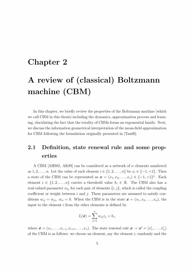
Chapter 2
A review of (classical) Boltzmann
machine (CBM)
In this chapter, we briefly review the properties of the Boltzmann machine (which
we call CBM in this thesis) including the dynamics, approximation process and learn-
ing, elucidating the fact that the totality of CBMs forms an exponential family. Next,
we discuss the information geometrical interpretation of the mean-field approximation
for CBM following the formulation originally presented in [Tan00].
2.1 Definition, state renewal rule and some prop-
erties
A CBM [AHS85, AK89] can be considered as a network of n elements numbered
as 1, 2, . . . , n. Let the value of each element i ∈ {1, 2, . . . , n} be xi ∈ {−1, +1}. Then
a state of the CBM can be represented as x = (x1, x2, . . . , xn) ∈ {−1, +1}n. Each
element i ∈ {1, 2, . . . , n} carries a threshold value hi ∈ R. The CBM also has a
real-valued parameter wij for each pair of elements {i, j}, which is called the coupling
coefficient or weight between i and j. These parameters are assumed to satisfy con-
ditions wij = wji, wii = 0. When the CBM is in the state x = (x1, x2, . . . , xn), the
input to the element i from the other elements is defined by
Ii(x̂) =n∑
j=1
wijxj + hi,
where x̂ = (x1, . . . , xi−1, xi+1, . . . , xn). The state renewal rule x → x′ = (x′1, . . . , x
′n)
of the CBM is as follows: we choose an element, say the element i, randomly and the
5
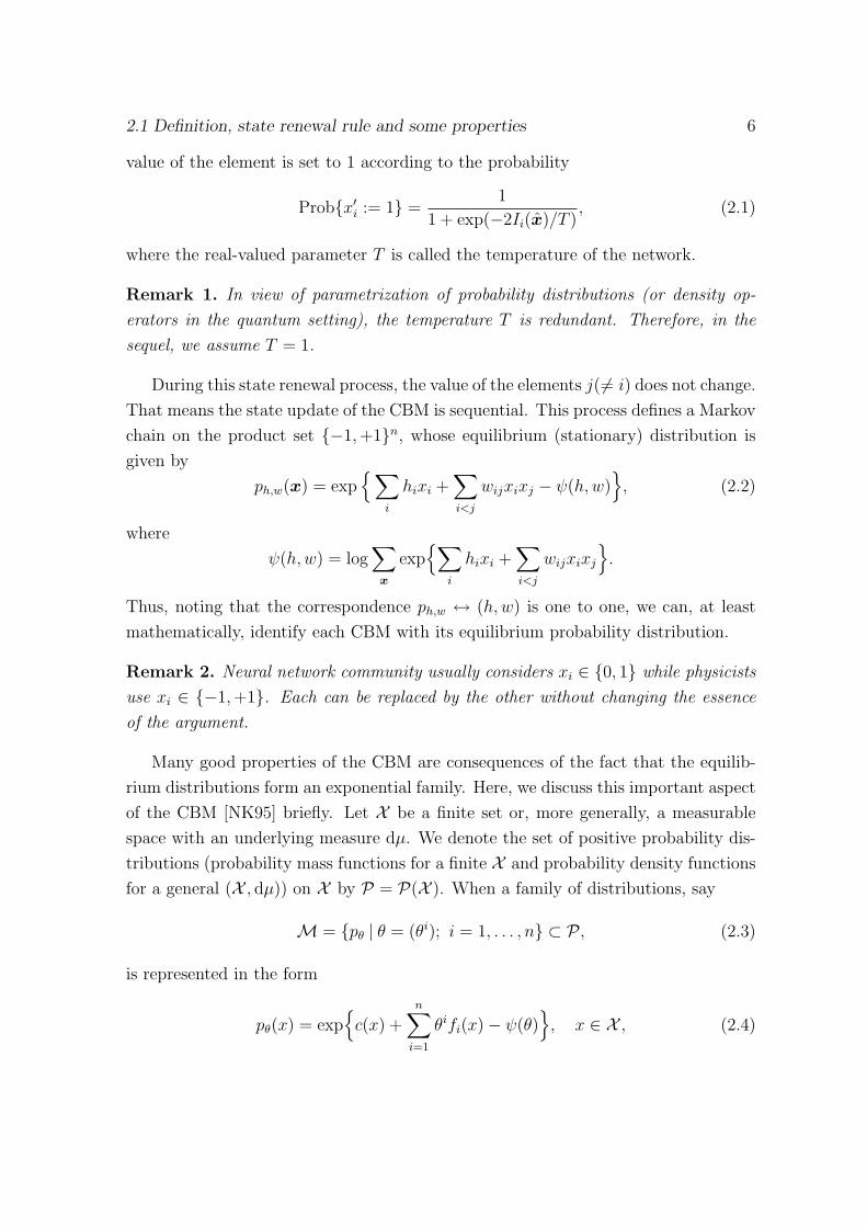
2.1 Definition, state renewal rule and some properties 6
value of the element is set to 1 according to the probability
Prob{x′i := 1} =
1
1 + exp(−2Ii(x̂)/T ), (2.1)
where the real-valued parameter T is called the temperature of the network.
Remark 1. In view of parametrization of probability distributions (or density op-
erators in the quantum setting), the temperature T is redundant. Therefore, in the
sequel, we assume T = 1.
During this state renewal process, the value of the elements j(6= i) does not change.
That means the state update of the CBM is sequential. This process defines a Markov
chain on the product set {−1, +1}n, whose equilibrium (stationary) distribution is
given by
ph,w(x) = exp{∑
i
hixi +∑i<j
wijxixj − ψ(h,w)}
, (2.2)
where
ψ(h,w) = log∑
x
exp{∑
i
hixi +∑i<j
wijxixj
}.
Thus, noting that the correspondence ph,w ↔ (h, w) is one to one, we can, at least
mathematically, identify each CBM with its equilibrium probability distribution.
Remark 2. Neural network community usually considers xi ∈ {0, 1} while physicists
use xi ∈ {−1, +1}. Each can be replaced by the other without changing the essence
of the argument.
Many good properties of the CBM are consequences of the fact that the equilib-
rium distributions form an exponential family. Here, we discuss this important aspect
of the CBM [NK95] briefly. Let X be a finite set or, more generally, a measurable
space with an underlying measure dµ. We denote the set of positive probability dis-
tributions (probability mass functions for a finite X and probability density functions
for a general (X , dµ)) on X by P = P(X ). When a family of distributions, say
M = {pθ | θ = (θi); i = 1, . . . , n} ⊂ P , (2.3)
is represented in the form
pθ(x) = exp{
c(x) +n∑
i=1
θifi(x) − ψ(θ)}
, x ∈ X , (2.4)
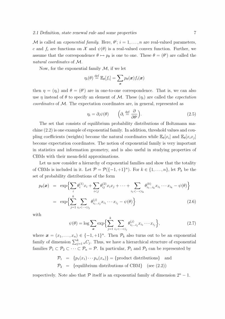
2.1 Definition, state renewal rule and some properties 7
M is called an exponential family. Here, θi; i = 1, . . . , n are real-valued parameters,
c and fi are functions on X and ψ(θ) is a real-valued convex function. Further, we
assume that the correspondence θ 7→ pθ is one to one. These θ = (θi) are called the
natural coordinates of M.
Now, for the exponential family M, if we let
ηi(θ)def= Eθ[fi] =
∑x
pθ(x)fi(x)
then η = (ηi) and θ = (θi) are in one-to-one correspondence. That is, we can also
use η instead of θ to specify an element of M. These (ηi) are called the expectation
coordinates of M. The expectation coordinates are, in general, represented as
ηi = ∂iψ(θ)(∂i
def=
∂
∂θi
). (2.5)
The set that consists of equilibrium probability distributions of Boltzmann ma-
chine (2.2) is one example of exponential family. In addition, threshold values and cou-
pling coefficients (weights) become the natural coordinates while Eθ[xi] and Eθ[xixj]
become expectation coordinates. The notion of exponential family is very important
in statistics and information geometry, and is also useful in studying properties of
CBMs with their mean-field approximations.
Let us now consider a hierarchy of exponential families and show that the totality
of CBMs is included in it. Let P = P({−1, +1}n). For k ∈ {1, . . . , n}, let Pk be the
set of probability distributions of the form
pθ(x) = exp{∑
i
θ(1)i xi +
∑i<j
θ(2)ij xixj + · · · +
∑i1<···<ik
θ(k)i1...ik
xi1 · · · xik − ψ(θ)}
= exp{ k∑
j=1
∑i1<···<ij
θ(j)i1...ij
xi1 · · · xij − ψ(θ)}
(2.6)
with
ψ(θ) = log∑
x
exp{ k∑
j=1
∑i1<···<ij
θ(j)i1...ij
xi1 · · · xij
}, (2.7)
where x = (x1, . . . , xn) ∈ {−1, +1}n. Then Pk also turns out to be an exponential
family of dimension∑k
j=1 nCj. Thus, we have a hierarchical structure of exponential
families P1 ⊂ P2 ⊂ · · · ⊂ Pn = P . In particular, P1 and P2 can be represented by
P1 = {p1(x1) · · · pn(xn)} = {product distributions} and
P2 = {equilibrium distributions of CBM} (see (2.2))
respectively. Note also that P itself is an exponential family of dimension 2n − 1.
2.2 Approximation process and learning 8
2.2 Approximation process and learning
Suppose that we are given an exponential family M ⊂ P of the form (2.4) and an
arbitrary probability distribution q ∈ P outside M. Let us consider the problem of
approximating q by an element pθ ∈ M. We adopt the Kullback-Leibler information
divergence
D(q‖pθ)def=
∑x
q(x) logq(x)
pθ(x)(2.8)
as the criterion of approximation. Our interest is to find θ which minimizes D(q‖pθ),
that is, arg minθ D(q‖pθ). Geometrically, this can be understood as the m-projection
defined in Subsection 2.3.2. Then, it is shown that
θ∗ = arg minθ
D(q‖pθ) ⇐⇒ ηi(θ∗) = Eq[fi], ∀i, (2.9)
where Eq denotes the expectation with respect to the probability distribution q. Ac-
tually, for any θ, we have
D(q‖pθ) = D(q‖pθ∗) + D(pθ∗‖pθ),
which is an example of the Pythagorean relation for D.
When a sequence of data x(1), . . . , x(N) is given, the approximation
minθ
D(q̂‖pθ)
of the empirical distribution
q̂ =1
N
N∑t=1
δx(t)
(where δx denotes the probability distribution satisfying δx(x) = 1) can be regarded
as a process of learning from the data. In particular, when the data x(1), . . . , x(N)
are assumed to be drawn from an unknown distribution in M, the learning turns out
to be the maximum likelihood estimation (MLE).
An algorithm for computing this approximation is the gradient method. In this
method, we assume that a positive-definite symmetric matrix [γij(θ)] ∈ Rn×n is spec-
ified for each point θ ∈ Rn, and a small positive constant ε is given in advance.
Then, starting from an arbitrary initial value θ, this process recurrently updates θ for
sufficiently many times according to
∆θi def= −ε
∑j
γij(θ)∂jD(q‖pθ), (2.10)
= ε∑
j
γij(θ){Eq[fj] − ηj(θ)}, (2.11)
2.2 Approximation process and learning 9
θi def= θi + ∆θi,
until ||∆θ|| becomes sufficiently small, which implies the convergence of pθ to pθ∗ .
Here, taking the value of ε smaller, the accuracy of approximation becomes better
but by that much the rate of convergence becomes slower.
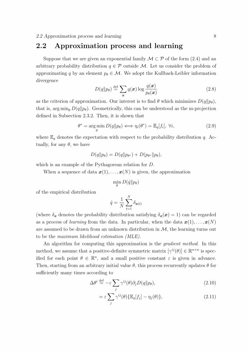
As a special case of this method, we obtain the learning algorithm for the CBM
proposed by Ackley et al. in [AHS85]. They showed that, setting the initial value
P
p(h,w)
M = P2
q
Figure 2.1: Approximation process for CBM.
of θ = {hi, wij} arbitrarily and going recursively updating this according to the
following equations, θ which minimizes D(q‖pθ) can be found approximately after
sufficient number of updates:
∆hidef= ε
(∑x
xiq(x) −∑
x
xipθ(x)
)(2.12)
= ε
(Eq[xi] − Eθ[xi]
)∆wij
def= ε
(∑x
xixjq(x) −∑
x
xixjpθ(x)
)(2.13)
= ε
(Eq[xixj] − Eθ[xixj]
)and
hidef= hi + ∆hi
wijdef= wij + ∆wij,
where Eq[·] and Eθ[·] represent the expectation values with respect to q and pθ respec-
tively. Equations (2.12) and (2.13) are nothing but (2.11) applied to M = P2 with
2.3 Mean-field approximation for CBMs 10
[γij(θ)] = [δij] (the Kronecker delta). On the other hand, a geometrically natural
choice of [γij(θ)] is [gij(θ)], which is the Fisher information matrix
gij(θ)def= Eθ[∂
i log pθ ∂j log pθ], ∂i =∂
∂ηi
(2.14)
for (ηi) or, equivalently is the inverse of the Fisher information matrix
gij(θ) = Eθ[∂i log pθ ∂j log pθ] (2.15)
for (θi) [AKN92]. This is an example of the so-called natural gradient method [Ama98].
2.3 Mean-field approximation for CBMs
In this section, first we give a brief introduction to the mean-field approximation
in statistical physics. Then we discuss some important points of the information
geometrical aspects of the mean-field approximation including both naive and higher-
order approximations for CBMs following [Tan00, AIS01]. We also briefly describe
the information geometrical viewpoint of the so-called Plefka expansion.
2.3.1 Introduction to mean-field approximation
Mean-field theory, dating back to Curie, Weiss and Ginzburg-Landau, is one of
the most common approaches to the study of complex physical systems. The basic
underlying idea is that the complicated interactions that each element of a complex
system is subjected to by its neighbors can be replaced by the interaction with an
effective (or mean) field. While mean-field approximation arose primarily in the field
of statistical mechanics, it provides an alternative perspective on the probabilistic
inference problem. For instance, it has more recently been applied for doing inference
in graphical models in artificial intelligence [JGJS99].
In magnetic materials the microscopic state of the system is supposed to be defined
by the values of local spin magnetizations. In many magnetic materials the electrons
responsible for the magnetic behavior are localized near the atoms of the crystal
lattice, and the force which tends to orient the spins is the (short range) exchange
interaction.
The most popular models, which describe this situation qualitatively are called
the Ising models. The microscopic variables in these systems are the Ising spins xi
which by definition can take only two values -1 or +1. The microscopic energy or the
2.3 Mean-field approximation for CBMs 11
Hamiltonian H as a function of all the Ising spins is given by
H = −∑i<j
Jijxixj − h∑
i
xi, (2.16)
where Jij are the values of the spin-spin interactions and h is the external magnetic
field. In particular, physicists usually consider nearest neighbor models for example,
the ferromagnetic Ising model with Jij > 0 and the anti-ferromagnetic Ising model
with Jij < 0. It is a well-known fact that in statistical physics, the thermal equilibrium
state of a system is given by the Boltzmann distribution
P (x) =1
Zexp
(−H(x)
T
), (2.17)
where T is the temperature∗ and
Z =∑
x
exp(−H(x)
T
)is a normalizing factor called the partition function. In spite of the apparent simplicity
of the Ising model, an exact solution (which means the calculation of the partition
function Z, expectations and the correlation functions) for the lattice system has
been found only for the one- and the two-dimensional cases in the zero external
magnetic field. In the higher dimensions one needs to use approximate methods.
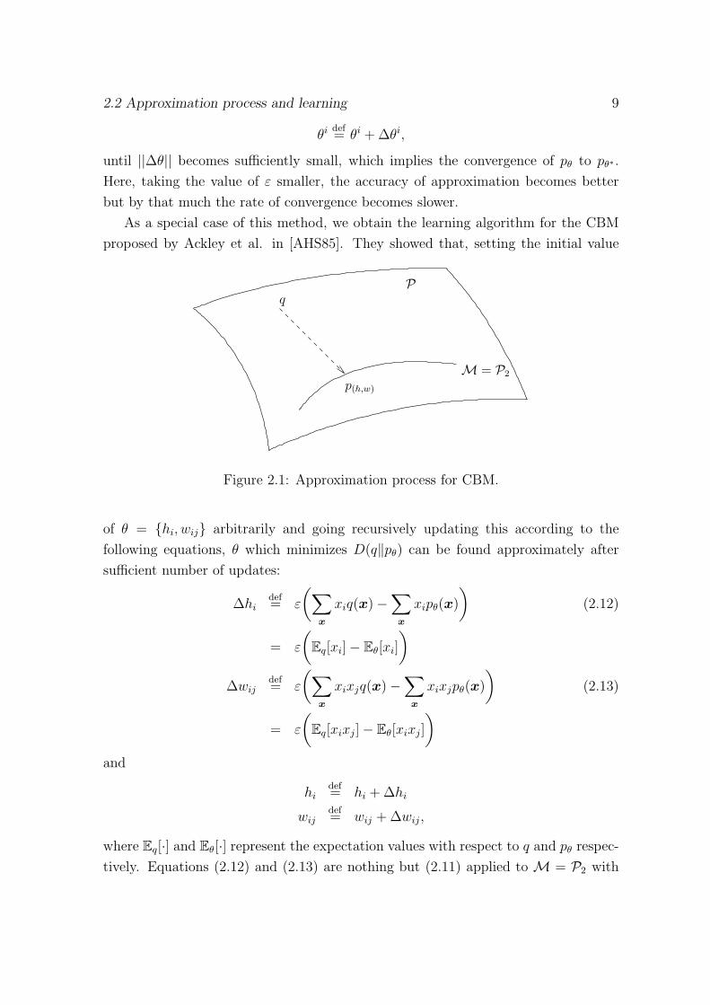
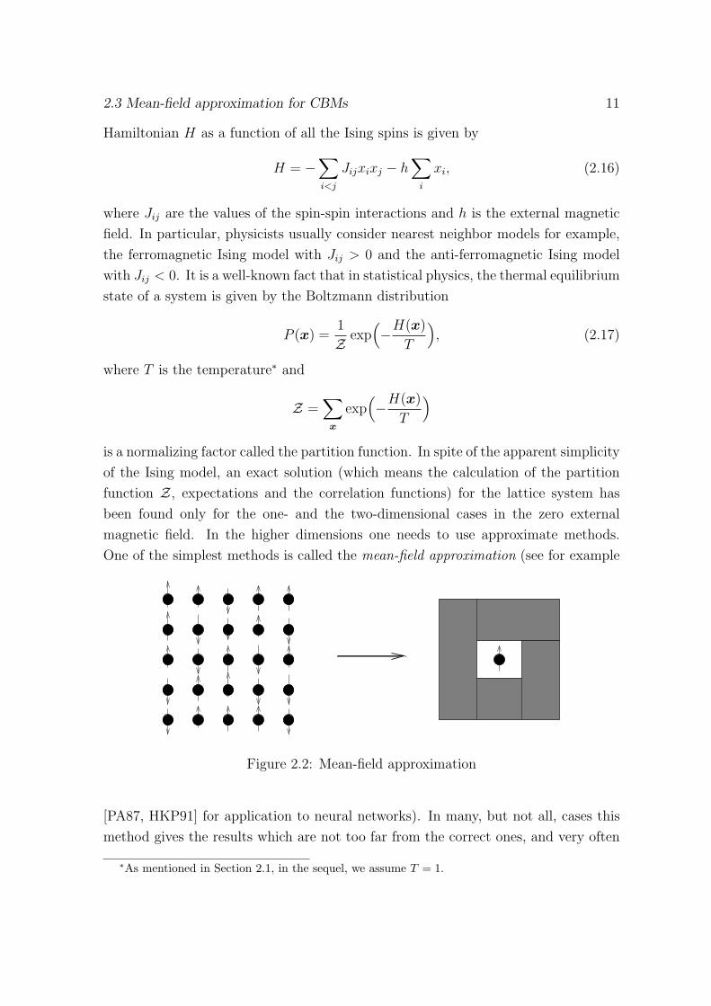
One of the simplest methods is called the mean-field approximation (see for example
Figure 2.2: Mean-field approximation
[PA87, HKP91] for application to neural networks). In many, but not all, cases this
method gives the results which are not too far from the correct ones, and very often
∗As mentioned in Section 2.1, in the sequel, we assume T = 1.
2.3 Mean-field approximation for CBMs 12
it makes possible to get some qualitative understanding of what is going on in the
system under consideration. The starting point of the mean-field approximation is
the fact that the joint distribution function of the non-interacting system can be
factorized as the product of the independent distribution functions in the individual
sites of the spin system.
2.3.2 Naive and higher-order mean-field approximations for
CBMs
In this subsection, we derive the naive mean-field equation and discuss briefly
the higher-order approximations based on the Plefka expansion from an information
geometrical point of view. The complete description of the information geometrical
interpretation of Plefka expansion is presented in the Chapter 5 for the quantum
setting.
Let us now recall P2, the manifold of CBMs. Here, we treat the case that each
element is subjected to different external magnetic fields (in the physical interpreta-
tion) hi which were considered equal to h in (2.16). Suppose that we are interested in
obtaining expectations mi with respect to a probability distribution in P2. However,
when the system size is large, the partition function exp(ψ(h,w)) is very difficult to
calculate and thus explicit calculation of the expectations mi is intractable. There-
fore, due to that difficulty, we are led to obtain a good approximation of mi for a
given probability distribution ph,w ∈ P2.
First, we consider the subspace P1 of P2. We parametrize each distribution in P1
by h̄ in order to distinguish from the parametrization in (2.2) and write as
ph̄(x) = exp{ ∑
i
h̄ixi − ψ(h̄)}
, (2.18)
where
ψ(h̄) =∑
i
log{
exp(h̄i) + exp(−h̄i)}
.
Then, P1 forms a submanifold of P2 specified by wij = 0 and h̄i as its coordinates.
The expectations m̄i := Eh̄[xi] form another coordinate system of P1. For a given
ph̄ ∈ P1, it is easy to obtain m̄i = Eh̄[xi] from h̄i because xi’s are independent. We
can calculate m̄i to be
m̄i =∂ψ(h̄)
∂h̄i
=exp(h̄i) − exp(−h̄i)
exp(h̄i) + exp(−h̄i)= tanh(h̄i), (2.19)
2.3 Mean-field approximation for CBMs 13
from which we obtain
h̄i =1
2log
(1 + m̄i
1 − m̄i
). (2.20)
The simple idea behind the mean field approximation for a ph,w ∈ P2 is to use
quantities obtained in the form of expectation with respect to some relevant ph̄ ∈ P1.
Now, we need a suitable criterion to measure the approximation of two probability
distributions. For the present purpose, we adopt the Kullback-Leibler divergence
(2.8). Given ph,w ∈ P2, its e-(exponential) and m-(mixture) projections (see [AN00])
onto P1 are defined by
p̄(e) = ph̄(e)def= arg min
ph̄∈P1
D(ph̄‖ph,w) (2.21)
and
p̄(m) = ph̄(m)def= arg min
ph̄∈P1
D(ph,w‖ph̄) (2.22)
respectively, where
h̄(e) = arg minh̄=(h̄i)
D(ph̄‖ph,w) (2.23)
and
h̄(m) = arg minh̄=(h̄i)
D(ph,w‖ph̄). (2.24)
As necessary conditions, we have
∂
∂h̄i
D(ph̄‖ph,w) = 0 (2.25)
and∂
∂h̄i
D(ph,w‖ph̄) = 0, (2.26)
which are weaker than (2.23) and (2.24). But sometimes (2.25) and (2.26) are chosen
to be the definitions of e-, m- projections respectively for convenience. It can be shown
that the m-projection p̄(m) gives the true values of expectations, that is mi = m̄i or
E(h,w)[xi] = Eh̄[xi] for ph̄ = p̄(m) (see (2.9)). It should be noted that the approximation
process in Section 2.2 can be considered as the m-projection from P onto P2. On
the other hand, the e-projection p̄(e) from P2 onto P1 gives the naive mean-field
approximation (see [Tan00]) which is explicitly given by
m̄i = tanh( ∑
j
wijm̄j + hi
), (2.27)
2.3 Mean-field approximation for CBMs 14
where m̄i = Eh̄[xi] for ph̄ = p̄(e). From (2.27) and (2.19), it is clear that in the
mean-field approximation the effective fields of other elements j(6= i) are replaced by
external fields called mean fields (see Figure 2.2).
Now we derive the naive mean-field equation for CBM. Recall that the equilibrium
distribution for CBM (2.2) is given by
pdef= ph,w(x) = exp
{∑i
hixi +∑i<j
wijxixj − ψ(h,w)}
, (2.28)
where
ψ(p)def= ψ(h,w) = log
∑x
exp{∑
i
hixi +∑i<j
wijxixj
}.
Now we define another function
φ(p) = φ(h,w)def=
∑i<j
wij Ep[xixj] +∑
i
hi Ep[xi] − ψ(p), (2.29)
which coincides with the negative entropy:
φ(p) =∑
x
p(x) log p(x). (2.30)
In particular, for a product distribution ph̄ ∈ P1, using Eh̄[xi] = m̄i , we have
φ(ph̄) =∑
i
[(1 + m̄i
2
)log
(1 + m̄i
2
)+
(1 − m̄i
2
)log
(1 − m̄i
2
)]. (2.31)
The KL divergence between p ∈ P2 and ph̄ ∈ P1 can be expressed in the following
form:
D(ph̄‖p) = ψ(p) + φ(ph̄) −∑i<j
wij Eh̄[xixj] −∑
i
hi Eh̄[xi]
= ψ(p) + φ(ph̄) −∑i<j
wijm̄im̄j −∑
i
him̄i.
= ψ(p) +1
2
∑i
[(1 + m̄i) log
(1 + m̄i
2
)+ (1 − m̄i) log
(1 − m̄i
2
)]−
∑i<j
wijm̄im̄j −∑
i
him̄i. (2.32)
Now consider the e-projection (2.25) from p ∈ P2 onto ph̄ ∈ P1, i.e.
∂
∂h̄i
D(ph̄‖p) = 0. (2.33)
2.3 Mean-field approximation for CBMs 15
Noting that h̄ and m̄ are in one-to-one correspondence, we may consider instead
∂
∂m̄i
D(ph̄‖p) = 0. (2.34)
Since ψ(p) does not depend on m̄i, we obtain from (2.32) that
0 =1
2log
(1 + m̄i
1 − m̄i
)−
∑j 6=i
wijm̄j − hi
= h̄i −∑j 6=i
wijm̄j − hi, (2.35)
where the second equality is from (2.20). Thus the naive mean-field equation is
obtained from (2.19) and (2.35) as
tanh−1(m̄i) =∑j 6=i
wijm̄j + hi (2.36)
and this is usually written in the form (2.27).
Let us briefly discuss the higher-order mean-field approximations for CBMs using
the information geometrical interpretation of the so-called Plefka expansion. Recall
that the elements of P2 are parametrized as ph,w by h = (hi) and w = (wij). This
means that (h,w) forms a coordinate system of the manifold P2. When P2 is viewed
as an exponential family, (h,w) turns out to be a natural coordinate system, while
the corresponding expectation coordinate system is given by (m, η) where m = (mi)
and η = (ηij) with mi = E(h,w)[xi]) and ηij = E(h,w)[xixj]) respectively. We now
define a third (or hybrid) coordinate system (m,w). The elements of P2 are then
parametrized by (m, w), which we denote by p̂m,w to avoid any confusion with ph,w.
Note that
P2 = {ph,w | (h,w) : free}= {p̂m,w | (m,w) : free} (2.37)
and that
p̂m,w = ph,w ⇐⇒ ∀i, mi = E(h,w)[xi]. (2.38)
One may think of obtaining the expectations mi by solving the equation
∂
∂mi
D(p̂m,w‖ph,w) = 0. (2.39)
The difficulty in this approach is that it is hard to derive the stationary condition
explicitly because p̂m,w is complex enough so that we cannot obtain an explicit ex-
pression for D(p̂m,w‖ph,w) in terms of {mi}. On the other hand, when w = 0 in the
2.3 Mean-field approximation for CBMs 16
first argument of D(p̂m,w‖ph,w), the equation (2.39) turns out to be
∂
∂mi
D(p̂m,0‖ph,w) = 0 (2.40)
which is nothing but the naive mean-field approximation discussed earlier.
The Plefka expansion was originally presented as a Taylor expansion of the Gibbs
potential [Ple82, Ple06]. The information geometrical interpretation of it is that to use
the Taylor expansion of the difference D(p̂m,0‖ph,w) − D(p̂m,w‖ph,w) up to a required
order of w to derive more precise approximations of {mi}. For the detailed discussion
of the information geometrical viewpoint of the Plefka expansion, see Chapter 5.
We mention, for example, the second-order mean-field equation
m̄i = tanh
(hi +
∑j 6=i
wijm̄j − m̄i
∑j 6=i
w2ij(1 − m̄2
j)
)(2.41)
which was originally derived by a different method in [TAP77]. Some other higher-
order terms have been calculated in [NT97].
Chapter 3
A quantum extension of CBM
We present a possible quantum extension of CBM which is called the quantum
Boltzmann machine (QBM). Furthermore, a subfamily of the totality of QBMs is
defined which is called the set of strongly separable QBMs (SSQBMs). A state renewal
rule is proposed for these states based on that for CBM. Note that, in this thesis, we
use the concepts of density operator, quantum measurement etc. without explicitly
describing their physical meaning and the interested reader is referred, for example,
to [NC02].
3.1 Definition of quantum Boltzmann machine (QBM)
Let us consider an n-element system of quantum Ising spins. Each element is
represented as a quantum bit (qubit) or quantum spin-12
with local Hilbert space C2,
and the n-element system corresponds to H ≡ (C2)⊗n ' C2n. Let S be the set of
faithful (strictly positive) states on H;
S = {ρ | ρ = ρ∗ > 0 and Tr ρ = 1}. (3.1)
Here, each ρ is a 2n × 2n matrix; ρ = ρ∗ > 0 means that ρ is Hermitian and strictly
positive or positive definite respectively; and Tr ρ = 1 shows that the trace of the
density matrix ρ is unity. Now corresponding to (2.6), an element of S is said to have
at most kth-order interactions if it is written as
ρθ = exp{∑
i,s
θ(1)is Xis +
∑i<j
∑s,t
θ(2)ijstXisXjt + · · ·
+∑
i1<···<ik
∑s1...sk
θ(k)i1...iks1...sk
Xi1s1 · · ·Xiksk− ψ(θ)
}17
3.1 Definition of quantum Boltzmann machine (QBM) 18
= exp{ k∑
j=1
∑i1<···<ij
∑s1...sj
θ(j)i1...ijs1...sj
Xi1s1 · · ·Xijsj− ψ(θ)
}(3.2)
with
ψ(θ) = log Tr exp{ k∑
j=1
∑i1<···<ij
∑s1...sj
θ(j)i1...ijs1...sj
Xi1s1 · · ·Xijsj
}, (3.3)
where Xis = I⊗(i−1) ⊗ Xs ⊗ I⊗(n−i), θ = (θ(j)i1...ijs1...sj
). Here, I is the identity matrix
on H and Xs for s ∈ {1, 2, 3} are the usual Pauli matrices given by
X1 =
(0 1
1 0
), X2 =
(0 −i
i 0
), X3 =
(1 0
0 −1
).
Letting Sk be the totality of states ρθ of the above form, we have the hierarchy
S1 ⊂ S2 ⊂ · · · ⊂ Sn = S. Note that S1 is the set of product states ρ1 ⊗ ρ2 ⊗ · · · ⊗ ρn.
Our main concern in the present chapter is S2. In the sequel, we let his = θ(1)is and
wijst = θ(2)ijst to rewrite (3.2) for k = 2 as
ρh,w = exp{∑
i,s
hisXis +∑i<j
∑s,t
wijstXisXjt − ψ(h,w)}
, (3.4)
where h = (his), w = (wijst). The real dimension of S2 is 3n(3n − 1)/2 which gives
the number of parameters to specify a density operator ρh,w.
Corresponding to the classical case, an element of S2 of the form (3.4) is called
a quantum Boltzmann machine or a QBM in this thesis (see also [YN05, YN06]),
although we have no quantum dynamics corresponding to the stochastic state change
of a CBM at present. Physically, a QBM simply means a general quantum state for
n-fold spins with at most second-order interactions which are arbitrary and determin-
istic, not random as in a spin glass.
Now, here we briefly discuss the set S1 for later use. The elements of S1 are
represented as ρh,0 by letting w = 0 in (3.4). In the sequel, we write them as
τh̄ = exp{ ∑
i,s
h̄isXis − ψ(h̄)}
(3.5)
by using new symbols τ and h̄ = (h̄is) when we wish to make it clear that we are
treating S1 instead of S2. We have
τh̄ =n⊗
i=1
exp{∑
s
h̄isXs − ψi(h̄i)}
, (3.6)
3.2 Strongly separable QBM (SSQBM) 19
where h̄i = (h̄is)s and
ψi(h̄i) = log Tr exp{∑
s
hisXs
}= log{exp(||h̄i||) + exp(−||h̄i||)} (3.7)
with ||h̄i||def=
√∑s(h̄is)2. Note that
ψ(h̄) =∑
i
ψi(h̄i). (3.8)
3.2 Strongly separable QBM (SSQBM)
3.2.1 Separability criterion and a state renewal rule
First, we review the state renewal process of the CBM. In Chapter 2, Section 2.1,
we mentioned that the probability distribution (2.2) is obtained as the equilibrium
distribution for the stochastic state renewal rule (2.1). The significance of this process
is its locality. That is, the random generation of data is simple and carried out by
each element based on the data sent from the other elements. The mathematical
essence of (2.1) is that it is the conditional distribution defined from (2.2). That is,
1
1 + exp(−2Ii(x̂))=
P (x1, . . . , xi = 1, . . . , xn)∑x′
iP (x1, . . . , x′
i, . . . , xn)
= P (xi = 1 | x1, . . . , xi−1, xi+1, . . . , xn).
This method to generate a random sequence X1, X2, . . . , Xn subject to P (x1, . . . , xn)
by the use of conditional distributions is generally called the Gibbs sampler (see
[GG84]) in classical mathematical statistics. The same idea is applied to a limited
class of QBMs.
Separability is a well-known concept in quantum information theory. For a state
ρ on the Hilbert space H = (C2)⊗n, it is called separable if there exist {λi}mi=1 ⊂ [0, 1]
and {τ (j)i }1≤i≤m,1≤j≤n ⊂ S(C2), such that
∑mi=1 λi = 1 and
ρ =m∑
i=1
λi τ(1)i ⊗ · · · ⊗ τ
(n)i . (3.9)
Separability is equivalent to the existence of finite sets X1, . . . ,Xn, a probability distri-
bution P = P (x1, . . . , xn) on X1 × · · · ×Xn and {τ (i)xi | xi ∈ Xi} ⊂ S(C2), i = 1, · · · , n,
such that
ρ =∑
x
P (x)τx, (3.10)
3.2 Strongly separable QBM (SSQBM) 20
where x = (x1, . . . , xn) and τx = τ(1)x1 ⊗ · · · ⊗ τ
(n)xn .
We can apply the method of Gibbs sampler to generate ρ in the form (3.10) as
follows:
State renewal rule:
(i) Choose i randomly.
(ii) Update xi ∈ Xi according to P (xi | x1, . . . , xi−1, xi+1, . . . , xn).
(iii) Set the state of i to τ(i)xi .
It is obvious that, according to the Gibbs sampler, the state converges to ρ by re-
peating this process for sufficiently many times.
3.2.2 Strongly separable states and SSQBM
Definition 1. A separable state ρ of the form (3.10) is called strongly separable if
[τ (i)xi
, τ(i)
x′i] = 0 ∀i, xi, x
′i ∈ Xi. (3.11)
This is equivalent to the existence of U = {u1, . . . , un}, where each ui is a unit
vector in R3, and a probability distribution P on {−1, +1}n such that
ρ =∑
x1,...,xn
P (x1, . . . , xn)πu1x1
⊗ · · · ⊗ πunxn
, (3.12)
where for any u = (u1, u2, u3) we define
πu1 =
1
2
[1 + u3 u1 − iu2
u1 + iu2 1 − u3
]=
1
2(I + u1X1 + u2X2 + u3X3)
πu−1 = π−u
1 = I − πu1 .
Note that πu = (πu1 , πu
−1) represents a projective measurement (projection-valued
measure, PVM) where πu1 and πu
−1 are mutually orthogonal projection operators sat-
isfying πu1 + πu
−1 = I. For a spin-12
particle, this PVM can be physically realized by
a Stern-Gerlach measurement of direction u. We call U = {ui} a frame of a strongly
separable state ρ.
Combination of steps (ii) and (iii) in the state renewal algorithm is equivalent to
setting the quantum state of ith element to
τ (i) = P (1 | x̂)πui1 + P (−1 | x̂)πui
−1
= Tr(i)[ρ′x̂],
3.2 Strongly separable QBM (SSQBM) 21
where (x̂ = (x1, . . . , x̂i, . . . , xn)), Tr(i) is the partial trace over n − 1 qubit systems
except for ith system,
ρ′x̂
def=
π̃x̂ρπ̃x̂
Tr[π̃x̂ρπ̃x̂]
and π̃x̂ = πu1x1
⊗ · · · ⊗ I ⊗ · · · ⊗ πunxn
where I is in the ith position. Note that ρ′x̂ is the
post measurement state of the target state ρ for the measurement results x̂.
Next theorem gives the necessary and sufficient conditions for a state of the form
(3.2) to be strongly separable.
Theorem 1. A state ρ represented in the form (3.2) in terms of the parameters
(θ(j)i1...ijs1...sj
) is strongly separable with frame U = {ui} iff there exists (θ(j)′i1...ij
) such
that ∀j,∀i1 < · · · < ∀ij,∀s1, . . . , ∀sj,
θ(j)i1...ijs1...sj
= θ(j)′i1...ij
ui1s1 · · · uijsj, (3.13)
where ui = (ui1, ui2, ui3).
Proof. First assume that (3.13) holds. Substituting, (3.13) to (3.2), we have
ρ = exp
[ k∑j=1
∑i1<···<ij
∑s1...sj
θ(j)i1...ijs1...sj
Xi1s1 . . . Xijsj− ψ(θ)
](3.14)
= exp
[ k∑j=1
∑i1<···<ij
θ(j)′i1···ijXi1ui1
. . . Xijuij− ψ(θ)
], (3.15)
where for any i and u = (us)3s=1 we define
Xiudef=
∑s
usXis
= I ⊗ · · · ⊗(∑
s
usXs
)⊗ · · · ⊗ I
= I ⊗ · · · ⊗ Xu ⊗ · · · ⊗ I
with Xudef=
∑s usXs = πu
1 − πu−1. Now, let for x = (x1, . . . , xn) ∈ {−1, +1}n,
f(x) =k∑
j=1
∑i1<···<ij
θ(j)′i1,...,ij
xi1 . . . xij . (3.16)
Then∑x
f(x)πu1x1
⊗ · · · ⊗ πunxn
=k∑
j=1
∑i1<···<ij
θ(j)′i1,··· ,ij
∑x
xi1 · · · xijπu1x1
⊗ · · · ⊗ πunxn
=k∑
j=1
∑i1<···<ij
θ(j)′i1...ij
Xi1ui1. . . Xijuij
. (3.17)
3.2 Strongly separable QBM (SSQBM) 22
Therefore, from (3.15) and (3.17)
ρ = exp
[∑x
f(x)πu1x1
⊗ · · · ⊗ πunxn
− ψ(θ)
]= exp
[∑x
{f(x) − ψ(θ)
}πu1
x1⊗ · · · ⊗ πun
xn
]=
∑x
exp[f(x) − ψ(θ)
]πu1
x1⊗ · · · ⊗ πun
xn
=∑
x
P (x)πu1x1
⊗ · · · ⊗ πunxn
, (3.18)
where
P (x) = exp[f(x) − ψ(θ)
]= exp
[ k∑j=1
∑i1,...,ij
θ(j)′i1<···<ij
xi1 . . . xij − ψ(θ)
]. (3.19)
Therefore ρ is strongly separable with frame U . Conversely, let us assume that ρ of the
form (3.2) is strongly separable with frame U . Then, by definition, ρ is represented as
(3.12) by a probability distribution P on {−1, +1}n. Since ρ is assumed to be faithful,
P (x) is positive for all x, and therefore P can be represented as (3.19) with k = n for
some θ′ = (θ(j)′i1,...,ij
). Then, tracing back the previous argument in the reverse order,
we have
ρ =∑
x
P (x)πu1x1
⊗ · · · ⊗ πunxn
= exp
[∑x
n∑j=1
∑i1<···<ij
θ(j)′i1...ij
xi1 . . . xijπu1x1
. . . πunxn
− ψ(θ)
]
= exp
[ n∑j=1
∑i1<···<ij
θ(j)′i1...ij
Xi1ui1. . . Xijuij
− ψ(θ)
]
= exp
[ n∑j=1
∑i1<···<ij
∑s1,··· ,sj
θ(j)′i1...ij
ui1s1 . . . uijsjXi1s1 . . . Xijsj
− ψ(θ)
]. (3.20)
Comparing (3.20) with (3.14), we have
θ(j)i1...ijs1...sj
= θ(j)′i1...ij
ui1s1 . . . uijsj(1 ≤ ∀j ≤ k)
and
θ(j)′i1...ij
= 0 if j > k.
which establishes the result.
3.2 Strongly separable QBM (SSQBM) 23
Let us now define S ′(U) as the set of strongly separable states ρ ∈ S with frame
U and S ′k(U)
def= S ′(U) ∩ Sk. Then we define the elements of the S ′
2(U) to be the
SSQBMs. First, we give a corollary of Theorem 1.
Corollary 1. A QBM ρθ, θ = (his, wijst), of the form (3.4) is strongly separable with
frame U = {ui} iff there exists θ′ = (h′i, w
′ij) such that ∀i, j, ∀s, t,
his = h′iuis, wijst = w′
ijuisujt, (3.21)
with ui = (ui1, ui2, ui3), which means that ρθ is represented as (3.12) with
P (x1, . . . , xn) = exp{∑
i
h′ixi +
∑i<j
w′ijxixj − ψ(h′, w′)
}. (3.22)
In particular, if hi 6= 0,∀i, the necessary and sufficient condition for a QBM ρθ to be
strongly separable (with some frame) is that
∀i, j, Wij ∝ hihTj , (3.23)
where
hi =
hi1
hi2
hi3
, Wij =
wij11 wij12 wij13
wij21 wij22 wij23
wij31 wij32 wij33
.
and T denotes the matrix transpose.
Proof. Obvious from the Theorem 1.
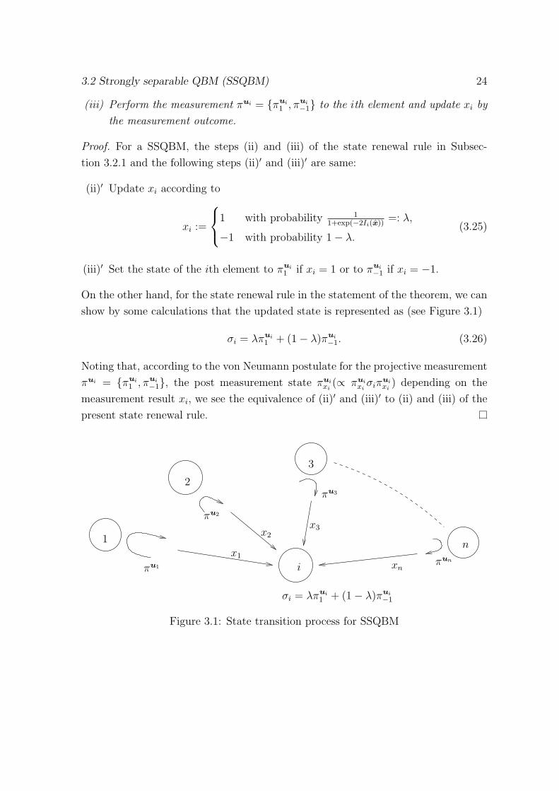
Next, we give a state renewal rule for the SSQBM in the following theorem.
Theorem 2. When the target state of a SSQBM is represented by (3.4) and (3.21),
the state renewal rule in Subsection 3.2.1 is carried out, starting from an arbitrary
initial state ρ ∈ S and arbitrary initial data x = (x1, . . . , xn) ∈ {−1, +1}n, by the
following procedure.
(i) Choose i randomly.
(ii) Using data x̂ = (x1, . . . , xi−1, xi+1, . . . , xn) available at the time, renew the state
of the ith element to
σi =1
2(I +
3∑s=1
visXs) (3.24)
with
vi = (vi1, vi2, vi3) = tanh
(∑j
w′ijxj + h′
i
)ui.
3.2 Strongly separable QBM (SSQBM) 24
(iii) Perform the measurement πui = {πui1 , πui
−1} to the ith element and update xi by
the measurement outcome.
Proof. For a SSQBM, the steps (ii) and (iii) of the state renewal rule in Subsec-
tion 3.2.1 and the following steps (ii)′ and (iii)′ are same:
(ii)′ Update xi according to
xi :=
1 with probability 11+exp(−2Ii(x̂))
=: λ,
−1 with probability 1 − λ.(3.25)
(iii)′ Set the state of the ith element to πui1 if xi = 1 or to πui
−1 if xi = −1.
On the other hand, for the state renewal rule in the statement of the theorem, we can
show by some calculations that the updated state is represented as (see Figure 3.1)
σi = λπui1 + (1 − λ)πui
−1. (3.26)
Noting that, according to the von Neumann postulate for the projective measurement
πui = {πui1 , πui
−1}, the post measurement state πuixi
(∝ πuixi
σiπuixi
) depending on the
measurement result xi, we see the equivalence of (ii)′ and (iii)′ to (ii) and (iii) of the
present state renewal rule.
1
2
3
n
i
x1
x2x3
xnπu1
πu2
πu3
πun
σi = λπui1 + (1 − λ)πui
−1
Figure 3.1: State transition process for SSQBM
Chapter 4
Geometry of quantum exponential
family and the space of QBMs
This chapter presents a discussion on the information geometrical structure of
the space of QBMs. First we introduce a quantum exponential family and discuss
its geometrical structure in general. Then it is shown that the space of QBMs can
be understood as one family in a hierarchical structure of exponential families. Fur-
thermore, the present chapter discusses the approximation processes for QBMs and
SSQBMs. Finally, we study the parameter estimation of SSQBM.
4.1 Quantum exponential families
We introduce a quantum version of exponential family (2.4) in the following. Let
H be a finite dimensional Hilbert space and denote the totality of faithful states on
H by
S = {ρ | ρ = ρ∗ > 0 and Tr ρ = 1}.
Suppose that a parametric family
M = {ρθ | θ = (θi); i = 1, . . . ,m} ⊂ S (4.1)
is represented in the form
ρθ = exp{
C +m∑
i=1
θiFi − ψ(θ)}
, (4.2)
where Fi (i = 1, . . . ,m), C are Hermitian operators and ψ(θ) is a real-valued function.
We assume in addition that the operators {F1, . . . , Fm, I}, where I is the identity
25
4.2 A metric and affine connections 26
operator, are linearly independent to ensure that the parametrization θ 7→ ρθ is one
to one. Then M forms an m-dimensional smooth manifold with a coordinate system
θ = (θi). In this thesis, we call such an M a quantum exponential family∗, or QEF
for short, with natural (or canonical) coordinates θ = (θi). It is easy to see that S is
a QEF of dimension (dimH)2 − 1. Note also that for any 1 ≤ k ≤ n the set Sk of
states (3.2) forms a QEF, including S2 of QBMs and S1 of product states.
If we let
ηi(θ)def= Tr
[ρθFi
], (4.3)
then η = (ηi) and θ = (θi) are in one-to-one correspondence. That is, we can also
use η instead of θ to specify an element of M. These (ηi) are called the expectation
coordinates of M.
In particular, the natural coordinates of S2 are given by (h,w) = (his, wijst) in
(3.4), while the expectation coordinates are (m,µ) = (mis, µijst) defined by
mis = Tr[ρh,w Xis] and µijst = Tr[ρh,w XisXjt]. (4.4)
On the other hand, the natural coordinates of S1 are h̄ = (h̄is) in (3.5), while the
expectation coordinates are m̄ = (m̄is) defined by
m̄is = Tr[τh̄Xis]. (4.5)
In this case, the correspondence between the two coordinate systems can explicitly
be represented as
m̄is =∂ψi(h̄i)
∂h̄is
=h̄is
||h̄i||tanh(||h̄i||) (4.6)
or as
h̄is =m̄is
||m̄i||tanh−1(||m̄i||), (4.7)
where ||m̄i||def=
√∑s(m̄is)2.
4.2 A metric and affine connections
In classical information geometry (see [AN00]), a Riemannian metric, called the
Fisher metric, and a one-parameter family of affine connections, called the α-connections∗It should be noted, however, (4.2) is merely one of the possible definitions of quantum exponential
family. Our definition has the advantage that it is closely related to the quantum relative entropy(4.25) and is completely analogous to the classical exponential family from a purely geometrical pointof view. On the other hand, it does not well fit to the framework of quantum estimation theory,which needs another definition of QEF such as the one based on symmetric logarithmic derivatives(see Section 7.4 of [AN00]).
4.2 A metric and affine connections 27
(α ∈ R), are canonically defined on an arbitrary manifold of probability distributions.
In particular, the (α = 1)-connection and the (α = −1)-connection, which are also
called the e-connection and m-connection respectively, together with the Fisher met-
ric have been shown very useful in many problems in statistics and other fields. In the
quantum case, on the other hand, we have infinitely many mathematical equivalents
of the Fisher metric and the α-connections including the e- and m-connections defined
on a manifold of quantum states. We introduce, in the present Section, an example of
quantum Fisher metric and e-, m-connections, and describe their properties, mainly
following [AN00]. Our choice of information geometrical structure has the advantage
that it is naturally linked with QEF and quantum relative entropy. For general terms
of differential geometry such as manifold, Riemannian metric and affine connection,
refer, for example, to [KN63].
Let H be a finite dimensional Hilbert space. We consider a d-dimensional para-
metric family
M = {ρθ | θ = (θ1, . . . , θd) ∈ Θ}, Θ ⊂ Rd
of faithful states on H. Then, θ = (θi); i = 1, . . . , d can be considered as a coordinate
system and M becomes a submanifold of the manifold of faithful states S on H. In
the following, we discuss the information geometrical structure of M including the
case M = S. As a first step, a Riemannian metric g = [gij] is defined on M by
gij(θ) = g(∂i, ∂j), where ∂idef=
∂
∂θi
=
∫ 1
0
Tr[ρλ
θ (∂i log ρθ)ρ1−λθ (∂j log ρθ)
]dλ (4.8)
= Tr[(∂iρθ)(∂j log ρθ)].
This is a quantum version of the Fisher information metric and is called the BKM
(Bogoliubov-Kubo-Mori) metric. Next, two torsion-free affine connections, the expo-
nential connection (or e-connection for short) ∇(e) and the mixture connection (or
m-connection for short) ∇(m), are defined on M as follows:
Γ(e)ij,k(θ)
def= g(∇(e)
∂i∂j, ∂k) = Tr[(∂i∂j log ρθ)(∂kρθ)] (4.9)
and
Γ(m)ij,k(θ)
def= g(∇(m)
∂i∂j, ∂k) = Tr[(∂i∂jρθ)(∂k log ρθ)], (4.10)
where g is the BKM metric. Note that both ∇(e) and ∇(m) are mappings (covariant
derivatives) which map two vector fields X,Y to ∇(e)X Y and to ∇(m)
X Y respectively.
4.3 Geometrical structure of the space of QBMs 28
The coefficients Γ(e)ij,k give a coordinate representation of the connection ∇(e) relative
to the metric g, while Γ(e)kij defined by
∇(e)∂i
∂j =∑
k
Γ(e)kij ∂k (4.11)
purely represent ∇(e). They are related to each other by
Γ(e)ij,k =
∑l
Γ(e)lij gkl.
Similarly, we have Γ(m)kij for ∇(m) such that
∇(m)∂i
∂j =∑
k
Γ(m)kij ∂k (4.12)
and
Γ(m)ij,k =
∑l
Γ(m)lij gkl.
These two connections ∇(e) and ∇(m) are dual with respect to the BKM metric
(4.8) in the sense that, for any vector fields X,Y, Z,
Xg(Y, Z) = g(∇(e)X Y, Z) + g(Y,∇(m)
X Z), (4.13)
or equivalently in the component form
∂igjk = Γ(e)ij,k + Γ
(m)ik,j. (4.14)
This kind of duality for affine connections plays a key role in classical and quantum
information geometry. Another notable relation between the two connections is
Γ(m)ij,k − Γ
(e)ij,k = Tijk, (4.15)
where
Tijk(θ)def= 2 Re
∫∫0≤ν≤λ≤1
Tr[ρν
θ(∂i log ρθ)ρλ−νθ (∂j log ρθ)ρ
1−λθ (∂k log ρθ)
]dν dλ. (4.16)
4.3 Geometrical structure of the space of QBMs
We have shown in Section 4.1 that the totality of QBMs form a QEF. In this
section, we describe the geometrical structure of QEF including the space of QBMs.
Let us now consider the case when M is a QEF (4.2) with natural coordinates θ =
4.3 Geometrical structure of the space of QBMs 29
(θi). It is then easy to check from (4.9) that the coefficients Γ(e)ij,k or Γ
(e)kij of the e-
connection are all zero. In the context of differential geometry, this means that M is
flat with respect to the connection ∇(e) (e-flat, for short) and θ = (θi) forms an affine
coordinate system for ∇(e) (e-affine coordinate system, for short). On the other hand,
the coefficients Γ(m)ij,k of the m-connection do not vanish with respect to the natural
coordinates θ = (θi). However, one of the remarkable consequences of the duality
(4.13) is that, if one of the two connections ∇(e) and ∇(m) is flat, then the other is
also flat, which is referred to as the dually flatness of the manifold with respect to the
information geometrical structure (g,∇(e),∇(m)). In the present case, the connection
coefficients of ∇(m) with respect to the expectation coordinates η = (ηi) defined by
(4.3) turns out to identically vanish. This means that M is m-flat with an m-affine
coordinate system (ηi). Moreover, we have
g
(∂
∂θi,
∂
∂ηj
)= δj
i (= 1 if i = j, 0 otherwise) (4.17)
and
ηi =∂ψ
∂θi, θi =
∂φ
∂ηi
, (4.18)
where ψ given in (4.2), is regarded as a function M → R by ψ(ρθ) = ψ(θ), and
φ : M → R is defined by the relation
φ(ρ) + ψ(ρ) =∑
i
ηi(ρ)θi(ρ), ∀ρ ∈ M. (4.19)
Note that equation (4.6) is an example of the first equation in (4.18). It can also be
shown that
φ(ρ) = −Tr[ρC] − S(ρ), (4.20)
where
S(ρ)def= −Tr[ρ log ρ] (4.21)
is the von Neumann entropy. In particular, for the QEF Sk of states (3.2), we have
C = 0 and hence φ(ρ) = −S(ρ). We note that the existence of m-affine coordinates
η = (ηi) and functions ψ, φ satisfying the relations (4.17), (4.18) and (4.19) is ensured
as a general property of dually flat space (see Theorem 3.6 in [AN00]), although it is
not difficult to directly verify these relations for a QEF (4.2).
Finally, let us rewrite (4.17) into a form which will be useful in later arguments.
Noting that (4.17) is written as
g
(∂
∂θi,
∂
∂ηj
)=
∂ηi
∂ηj
(4.22)
4.4 Geometry of quantum relative entropy 30
and that
{(∂
∂ηj
)ρ
}form a basis of the tangent space Tρ(M), we have
g
(( ∂
∂θi
)ρ, ∂′
)= ∂′ηi ∀∂′ ∈ Tρ(M). (4.23)
Similarly, we have
g
(( ∂
∂ηi
)ρ, ∂′
)= ∂′θi ∀∂′ ∈ Tρ(M), (4.24)
although we use only (4.23) in this thesis.
4.4 Geometry of quantum relative entropy
In this section, we focus on the quantum relative entropy
D(ρ‖σ)def= Tr[ρ(log ρ − log σ)] (4.25)
for two density operators ρ, σ ∈ M and describe its properties related to the dually
flat structure (g,∇(e),∇(m)) of a QEF M as the continuation of the previous section.
First, we note that the relation
D(ρ‖σ) = φ(ρ) + ψ(σ) −∑
i
ηi(ρ)θi(σ) (4.26)
holds for any ρ, σ ∈ M with ψ and φ defined in (4.18) and (4.19). From this, we have
D(ρ‖σ) + D(σ‖τ) − D(ρ‖τ) =∑
i
{ηi(ρ) − ηi(σ)}{θi(τ) − θi(σ)}. (4.27)
Moreover, it can be shown that (4.27), with the positivity
D(ρ‖σ) ≥ 0, D(ρ‖σ) = 0 iff ρ = σ, (4.28)
completely characterizes the quantum relative entropy D.
Let us clarify the geometrical meaning of the right hand side of (4.27). In gen-
eral, given a coordinate system ξi and an affine connection ∇ with coefficients Γkij, a
geodesic with respect to ∇ is defined by the second order ordinary differential equation
ξ̈k +∑i,j
Γkij ξ̇
iξ̇j = 0. (4.29)
4.4 Geometry of quantum relative entropy 31
If, in addition, ξi is an affine coordinate system with respect to a flat ∇, the equation
becomes ξ̈k = 0 or equivalently
ξit = tξi
0 + (1 − t)ξi1. (4.30)
In particular, an e-geodesic in the QEF (4.2) is given by
θit = tθi
0 + (1 − t)θi1. (4.31)
This turns out to be equivalent to
log ρt = t log ρ0 + (1 − t) log ρ1 − ψ(t),
where ψ(t) is the normalization constant. In other words, an e-geodesic of a QEF is
itself a one dimensional QEF. On the other hand, an m-geodesic is represented as
ηti = tη0i + (1 − t)η1i. (4.32)
If we consider the case M = S, the m-geodesic can be written as
ρt = tρ0 + (1 − t)ρ1. (4.33)
Such a family of states {ρt} is called a (one dimensional) mixture family, which is
related to the origin of the name “mixture connection”, but note that (4.32) is not
generally represented as (4.33) unless M = S.
Let γ : [0, 1] → M be an m-geodesic such that γ(0) = σ, γ(1) = ρ and δ : [0, 1] →M be an e-geodesic such that δ(0) = σ, δ(1) = τ . Then, from (4.31) and (4.32) we
obtain
γ̇(0) =∑
i
{ηi(ρ) − ηi(σ)}( ∂
∂ηi
)σ∈ Tσ(M) (4.34)
and
δ̇(0) =∑
i
{θi(τ) − θi(σ)}( ∂
∂θi
)σ∈ Tσ(M). (4.35)
Hence, from (4.17) we have
g(γ̇(0), δ̇(0)) =∑
i
{ηi(ρ) − ηi(σ)}{θi(τ) − θi(σ)} (4.36)
which coincides with the right hand side of (4.27). We thus obtain the following
theorem:
4.4 Geometry of quantum relative entropy 32
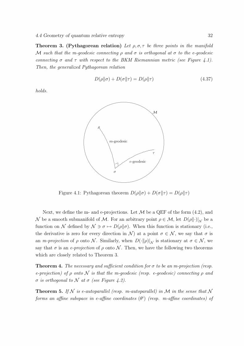
Theorem 3. (Pythagorean relation) Let ρ, σ, τ be three points in the manifold
M such that the m-geodesic connecting ρ and σ is orthogonal at σ to the e-geodesic
connecting σ and τ with respect to the BKM Riemannian metric (see Figure 4.1).
Then, the generalized Pythagorean relation
D(ρ‖σ) + D(σ‖τ) = D(ρ‖τ) (4.37)
holds.
ρ
σ
τ
m-geodesic
e-geodesic
M
Figure 4.1: Pythagorean theorem D(ρ‖σ) + D(σ‖τ) = D(ρ‖τ)
Next, we define the m- and e-projections. Let M be a QEF of the form (4.2), and
N be a smooth submanifold of M. For an arbitrary point ρ ∈ M, let D(ρ‖·)|N be a
function on N defined by N 3 σ 7→ D(ρ‖σ). When this function is stationary (i.e.,
the derivative is zero for every direction in N ) at a point σ ∈ N , we say that σ is
an m-projection of ρ onto N . Similarly, when D(·‖ρ)|N is stationary at σ ∈ N , we
say that σ is an e-projection of ρ onto N . Then, we have the following two theorems
which are closely related to Theorem 3.
Theorem 4. The necessary and sufficient condition for σ to be an m-projection (resp.
e-projection) of ρ onto N is that the m-geodesic (resp. e-geodesic) connecting ρ and
σ is orthogonal to N at σ (see Figure 4.2).
Theorem 5. If N is e-autoparallel (resp. m-autoparallel) in M in the sense that Nforms an affine subspace in e-affine coordinates (θi) (resp. m-affine coordinates) of

4.5 Approximation processes for QEF and SSQBM 33
M, then an m-projection (resp. e-projection) is unique and attains the minimum of
D(ρ‖·)|N (resp. D(·‖ρ)|N ). Note that an e-autoparallel submanifold is nothing but a
QEF.
Remark 3. For proofs of the Theorem 3, Theorem 4 and Theorem 5, refer to [AN00].
ρ
σ
N
M
Figure 4.2: Projection σ from ρ ∈ M to N
Finally, we note another property of D for later use. We have the Taylor expansion
of D(ρ‖σ) (see [AN00], p 55) as
D(ρ‖σ)def=
1
2
∑ij
gij(ρ)∆θi∆θj +1
6
∑ijk
hijk(ρ)∆θi∆θj∆θk + · · · , (4.38)
where ∆θi def= θi(σ)−θi(ρ). Here, the second-order coefficients gij are the components
of the BKM metric and the third-order coefficients hijk are determined from gij and
the connection coefficients by
hijkdef= ∂igjk + Γ
(e)jk,i = Γ
(e)ij,k + Γ
(m)ik,j + Γ
(e)jk,i, (4.39)
where the second equality is due to (4.14).
4.5 Approximation processes for QEF and SSQBM
The purpose of this section is to discuss the approximation processes for QEF and
SSQBM corresponding to that for CBM. We also study the parameter estimation of
4.5 Approximation processes for QEF and SSQBM 34
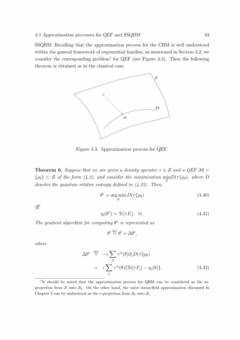
SSQBM. Recalling that the approximation process for the CBM is well understood
within the general framework of exponential families, as mentioned in Section 2.2, we
consider the corresponding problem† for QEF (see Figure 4.3). Then the following
theorem is obtained as in the classical case.
S
τ
ρθ
M
Figure 4.3: Approximation process for QEF.
Theorem 6. Suppose that we are given a density operator τ ∈ S and a QEF M =
{ρθ} ⊂ S of the form (4.2), and consider the minimization minθ
D(τ‖ρθ), where D
denotes the quantum relative entropy defined in (4.25). Then,
θ∗ = arg minθ
D(τ‖ρθ) (4.40)
iff
ηi(θ∗) = Tr[τFi], ∀i. (4.41)
The gradient algorithm for computing θ∗ is represented as
θi def= θi + ∆θi,
where
∆θi def= −ε
∑β
γij(θ)∂jD(τ‖ρθ)
= ε∑
j
γij(θ){Tr[τFj] − ηj(θ)}. (4.42)
†It should be noted that the approximation process for QBM can be considered as the m-projection from S onto S2. On the other hand, the naive mean-field approximation discussed inChapter 5 can be understood as the e-projection from S2 onto S1
4.5 Approximation processes for QEF and SSQBM 35
Let us now consider the geometrical structure of the space of SSQBMs. Following
the definition of SSQBM in Section 3.2, we have natural diffeomorphisms S ′(U) ' Pand S ′
k(U) ' Pk. We give the following theorem which describes the information
geometrical structure of S ′k(U).
Theorem 7. For an arbitrary frame U , S ′k(U) is a QEF and therefore is autoparallel
in S with respect to the e-connection (e-autoparallel). The induced information geo-
metrical structure (g,∇(e),∇(m)) on S ′k(U) is dually flat and is equivalent to that of
Pk.
Proof. Obvious from the fact that an element of S ′k(U) is represented as (see the proof
of Theorem 1 in Subsection 3.2.2)
ρ =∑
x1,...,xn
P (x1, . . . , xn)πu1x1
⊗ · · · ⊗ πunxn
= exp
[ n∑j=1
∑i1<···<ij
θ(j)′i1...ij
Xi1ui1. . . Xijuij
− ψ(θ′)
](4.43)
by P ∈ Pk and θ′ = (θ(j)′i1,...,ij
).
We now revisit the approximation process for SSQBMs (see Figure 4.4). Suppose
that we are given a density operator τ ∈ S, and consider the problem of approximating
τ by a SSQBM in S ′2(U) = {ρθ′}, where U = {ui} is an arbitrarily fixed frame. Let
τ ′ def=
∑x
π̃Ux τ π̃U
x =∑
x
Tr[τ π̃U
x
]π̃U
x ∈ S ′(U),
where π̃Ux = πu1
x1⊗ · · · ⊗ πun
xnfor x = (x1, . . . , xn). Then we obtain
Tr[τ π̃Ux ] = Tr[τ ′π̃U
x ], ∀ x (4.44)
from which it implies
Tr[τ(log σ − log τ ′)] = Tr[τ ′(log σ − log τ ′)], ∀ σ ∈ S ′(U). (4.45)
The above equation is rewritten as Tr(τ − τ ′)(log σ − log τ ′) = 0, which equals to
D(τ‖τ ′) + D(τ ′‖σ) − D(τ‖σ) = Tr(τ − τ ′)(log σ − log τ ′) = 0. (4.46)
Thus we obtain the Pythagorean relation
D(τ‖σ) = D(τ‖τ ′) + D(τ ′‖σ) (4.47)
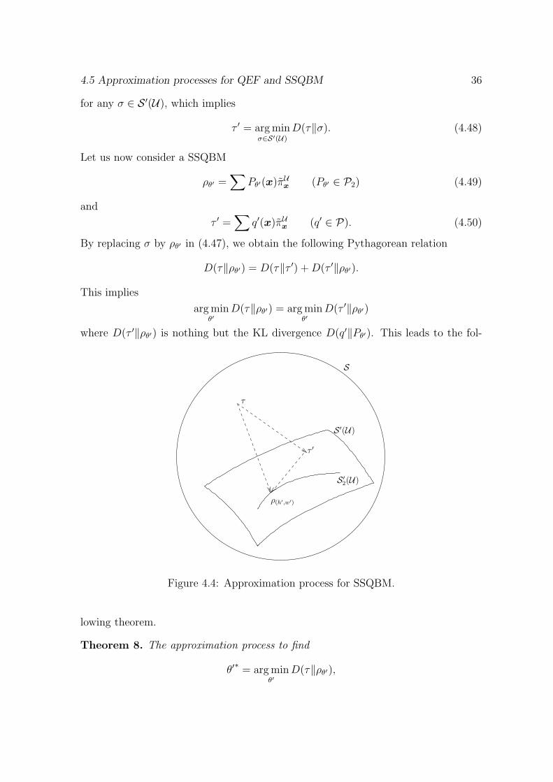
4.5 Approximation processes for QEF and SSQBM 36
for any σ ∈ S ′(U), which implies
τ ′ = arg minσ∈S′(U)
D(τ‖σ). (4.48)
Let us now consider a SSQBM
ρθ′ =∑
Pθ′(x)π̃Ux (Pθ′ ∈ P2) (4.49)
and
τ ′ =∑
q′(x)π̃Ux (q′ ∈ P). (4.50)
By replacing σ by ρθ′ in (4.47), we obtain the following Pythagorean relation
D(τ‖ρθ′) = D(τ‖τ ′) + D(τ ′‖ρθ′).
This implies
arg minθ′
D(τ‖ρθ′) = arg minθ′
D(τ ′‖ρθ′)
where D(τ ′‖ρθ′) is nothing but the KL divergence D(q′‖Pθ′). This leads to the fol-
S
τ
τ′
S ′(U)
S′
2(U)
ρ(h′,w′)
Figure 4.4: Approximation process for SSQBM.
lowing theorem.
Theorem 8. The approximation process to find
θ′∗
= arg minθ′
D(τ‖ρθ′),
4.5 Approximation processes for QEF and SSQBM 37
where θ′ = (h′, w′), is decomposed into two parts:
τ ′ = arg minσ∈S′(U)
D(τ‖σ)
and
θ′∗
= arg minθ′
D(τ ′‖ρθ′).
The second part turns out to be equivalent to the approximation problem for the CBM
addressed in Section 2.2 by S ′2(U) ' P2.
Finally, in this section, we consider the parameter estimation of SSQBMs. Sup-
pose that we are given N independent quantum systems, each of which is a SSQBM
ρθ′ (θ′ = (h′i, w
′ij)) with frame U and that we perform a projective measurement πU
on each SSQBM given by the PVM
πUdef= {π̃U
x}x∈{−1,+1}n , (4.51)
where π̃Ux = πu1
x1⊗πu2
x2⊗πun
xnfor x = (x1, . . . , xn), to yield a set of data {x(1), . . . , x(N)}.
Let P̂ denote the empirical distribution of {x(t)}Nt=1 and let
τ̂def=
∑x
P̂ (x)π̃Ux . (4.52)
Then, recalling that an SSQBM ρθ′ ∈ S ′2(U) is represented as
ρθ′ =∑
x
Pθ′(x)π̃Ux (4.53)
by a CBM Pθ′ , we have
θ̂′def= θ̂′MLE(x(1), . . . , x(N))
= arg maxθ′
Pθ′(x(1))Pθ′(x(2)) · · ·Pθ′(x(N))
= arg minθ′
D(P̂‖Pθ′)
= arg minθ′
D(τ̂‖ρθ′). (4.54)
This means that the MLE for the data is given by the approximation process for τ̂ .
Chapter 5
Information geometry of mean-field
approximation for QBMs
This chapter discusses the information geometrical interpretation of the mean-
field approximation for QBMs. First we derive the naive mean-field equation for
QBMs using the concepts of e- and m- projections. Then the higher-order corrections
are discussed noting the correspondence of the coefficients of Plefka expansion to
the information geometrical quantities of a Taylor expansion of the quantum relative
entropy.
5.1 The e-, m-projections and naive mean-field ap-
proximation
In this section, we derive the naive mean-field equation for QBMs explicitly from
the viewpoint of information geometry. Suppose that we are interested in calculating
the expectations mis = Tr[ρh,wXis] from given (h,w) = (his, wijst). Since the direct
calculation is intractable in general when the system size is large, we need to em-
ploy a computationally efficient approximation method. Mean-field approximation
is a well-known technique for this purpose. The simple idea behind the mean-field
approximation for a ρh,w ∈ S2 is to use quantities obtained in the form of expectation
with respect to some relevant τh̄ ∈ S1. As explained in the Chapter 1, T. Tanaka
[Tan96, Tan00] has elucidated the essence of the naive mean-field approximation for
classical spin models in terms of e-, m-projections. Our aim is to extend this idea to
quantized spin models.
In the following arguments, we regard S2 as a QEF with the natural coordinates
38
5.1 The e-, m-projections and naive mean-field approximation 39
(θα) = (his, wijst) and the expectation coordinates (ηα) = (mis, µijst) (see (4.4)),
where α is an index denoting α = (i, s) or α = (i, j, s, t). First, let us consider the
m-projection onto S1 and show that it preserves the expectations mis. Note that
since S1 is e-autoparallel in S2, the m-projection is unique and attains the minimum
of D by Theorem 5. Suppose ρ = ρh,w ∈ S2 is given and τ ∈ S1 be its m-projection.
Let γ be the m-geodesic such that γ(1) = ρ, γ(0) = τ . Then, from (4.32) we have
ηα(γ(t)) = t ηα(ρ) + (1 − t) ηα(τ), (5.1)
and, in particular,
mis(γ(t)) = tmis(ρ) + (1 − t) mis(τ). (5.2)
Hence, substituting θi := his, ηi := mis, ∂′ := γ̇(0) and ρ := τ into (4.23) we get
g
(( ∂
∂his
)τ, γ̇(0)
)=
dmis(γ(t))
dt
∣∣∣∣t=0
= mis(ρ) − mis(τ). (5.3)
Since
Tτ (S1) = span
{( ∂
∂his
)τ
}, (5.4)
it follows from (5.3) and Theorem 4 that mis(ρ) = mis(τ). This means that the
expectation values do not change if we use the m-projection.
Next, we show that the naive mean-field equation is derived by considering e-
projection. Suppose that τ = τh̄ ∈ S1 is an e-projection of ρ = ρh,w ∈ S2 onto S1,
and let γ be the e-geodesic such that γ(1) = ρ, γ(0) = τ . Note that from (4.31)
dθα(γ(t))
dt
∣∣∣∣t=0
= θα(ρ) − θα(τ), (5.5)
i.e.,
dhis(γ(t))
dt
∣∣∣∣t=0
= his(ρ) − his(τ) = his − h̄is (5.6)
dwijst(γ(t))
dt
∣∣∣∣t=0
= wijst(ρ) = wijst since wijst(τ) = 0. (5.7)
Now, recall that (m̄is) defined by (4.5) form a coordinate system of S1, so that
Tτ (S1) = span
{( ∂
∂m̄is
)τ
}is
. (5.8)
5.2 Plefka expansion and higher-order mean-field approximations 40
Hence it follows from Theorem 4 that, ∀i, s,
0 = g
(γ̇(0),
( ∂
∂m̄is
)τ
)=
∑α
dθα(γ(t))
dt
∣∣∣∣t=0
g
(( ∂
∂θα
)τ,( ∂
∂m̄is
)τ
)=
∑α
dθα(γ(t))
dt
∣∣∣∣t=0
( ∂ηα
∂m̄is
)τ
(from (4.23))
=∑j,t
(hjt − h̄jt)∂mjt
∂m̄is
+∑j<k
∑t,u
wjktu∂µjktu
∂m̄is
= his − h̄is +∑
(i<)k,u
wiksum̄ku +∑
(i>)j,t
wjitsm̄jt
(since mjt = m̄jt and µjktu = m̄jtm̄ku on S1)
= his − h̄is +∑j,t
wijstm̄jt,
where the last equality follows by letting
wiistdef= 0 and wijst
def= wjits (i > j). (5.9)
We thus obtain
h̄is = his +∑j,t
wijstm̄jt. (5.10)
Both (4.6) (or (4.7)) and (5.10) together give the naive mean-field equation for QBMs.
It should be remarked that this naive mean-field equation may have several solutions
{h̄is} for a given set of {his, wijst} as in the classical case, which correspond to the
fact that e-projection onto an e-autoparallel submanifold is not unique in general.
In this section, we have shown some properties of m- and e-projections based on the
geometrical characterization given in Theorem 4, but note that the same properties
can also be derived in several different ways; for instance, we can use the relations
(4.18)-(4.19) and (4.26) for ψ and φ to derive them as was shown for the classical
case in Subsection 2.3.2.
5.2 Plefka expansion and higher-order mean-field
approximations
Although the naive mean-field approximation is used extensively as a common
tool to compute characteristic quantities of multi-particle systems, it is necessary
5.2 Plefka expansion and higher-order mean-field approximations 41
to consider higher-order mean-field approximations to improve the accuracy in some
situations. In this section, we discuss a method to derive higher-order mean-field
approximations which utilizes a Taylor expansion of the quantum relative entropy.
This coincides with the Plefka expansion of the Gibbs potential as pointed out at the
end of the Section. We elucidate the correspondence of the coefficients of the Taylor
expansion to the information geometrical quantities such as the metric and the e-,
m-connections.
We start the discussion of higher-order approximations by recalling that the ele-
ments of S2 are parametrized as ρh,w by h = (his) and w = (wijst). This means that
(θα) = (h,w) forms a coordinate system of the manifold S2. In viewing S2 as a QEF,
(h,w) is a natural coordinate system, while the corresponding expectation coordinate
system is given by (ηα) = (m,µ) with m = (mis) and η = (ηijst). Let us now define
a third (or hybrid) coordinate system (ξα)def= (m, w). The elements of S2 are then
parametrized by (m,w), which we denote by ρ̂m,w to avoid confusion with ρh,w. Note
that
S2 = {ρh,w | (h,w) : free} = {ρ̂m,w | (m,w) : free} (5.11)
and that
ρ̂m,w = ρh,w ⇐⇒ ∀i, ∀s, mis = Tr[ρh,wXis]. (5.12)
For an arbitrarily fixed w, a submanifold of S2 is defined by
F(w)def= {ρh,w | h : free} = {ρ̂m,w | m : free}. (5.13)
As a special case we have
F(0) = {ρh,0 | h : free} = {ρ̂m,0 | m : free} = S1
which is the manifold of product states. We see that the family {F(w)}w forms a
foliation of S2 as
S2 =∪w
F(w). (5.14)
Similarly, for an arbitrarily fixed m we define
A(m)def= {ρ̂m,w | w : free}= {ρ ∈ S2 | ∀i, ∀s, mis = Tr[ρXis]}, (5.15)
which yields another foliation of S2 as
S2 =∪m
A(m). (5.16)
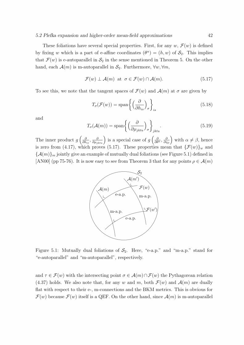
5.2 Plefka expansion and higher-order mean-field approximations 42
These foliations have several special properties. First, for any w, F(w) is defined
by fixing w which is a part of e-affine coordinates (θα) = (h,w) of S2. This implies
that F(w) is e-autoparallel in S2 in the sense mentioned in Theorem 5. On the other
hand, each A(m) is m-autoparallel in S2. Furthermore, ∀w,∀m,
F(w) ⊥ A(m) at σ ∈ F(w) ∩ A(m). (5.17)
To see this, we note that the tangent spaces of F(w) and A(m) at σ are given by
Tσ(F(w)) = span
{( ∂
∂his
)σ
}is
(5.18)
and
Tσ(A(m)) = span
{( ∂
∂µjktu
)σ
}jktu
. (5.19)
The inner product g(
∂∂his
, ∂∂µjktu
)is a special case of g
(∂
∂θα , ∂∂ηβ
)with α 6= β, hence
is zero from (4.17), which proves (5.17). These properties mean that {F(w)}w and
{A(m)}m jointly give an example of mutually dual foliations (see Figure 5.1) defined in
[AN00] (pp 75-76). It is now easy to see from Theorem 3 that for any points ρ ∈ A(m)
A(m)
S2
A(m′)
F(w)
e-a.p.
m-a.p.
e-a.p. m-a.p.
F(w′)
Figure 5.1: Mutually dual foliations of S2. Here, “e-a.p.” and “m-a.p.” stand for
“e-autoparallel” and “m-autoparallel”, respectively.
and τ ∈ F(w) with the intersecting point σ ∈ A(m)∩F(w) the Pythagorean relation
(4.37) holds. We also note that, for any w and m, both F(w) and A(m) are dually
flat with respect to their e-, m-connections and the BKM metrics. This is obvious for
F(w) because F(w) itself is a QEF. On the other hand, since A(m) is m-autoparallel
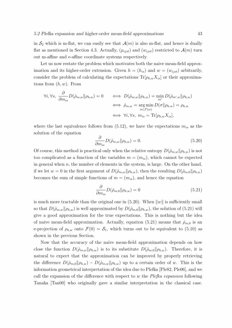
5.2 Plefka expansion and higher-order mean-field approximations 43
in S2 which is m-flat, we can easily see that A(m) is also m-flat, and hence is dually
flat as mentioned in Section 4.3. Actually, (µijst) and (wijst) restricted to A(m) turn
out m-affine and e-affine coordinate systems respectively.
Let us now restate the problem which motivates both the naive mean-field approx-
imation and its higher-order extension. Given h = (his) and w = (wijst) arbitrarily,
consider the problem of calculating the expectations Tr[ρh,wXis] or their approxima-
tions from (h,w). From
∀i, ∀s,∂
∂mis
D(ρ̂m,w‖ρh,w) = 0 ⇐⇒ D(ρ̂m,w‖ρh,w) = minm′
D(ρ̂m′,w‖ρh,w)
⇐⇒ ρ̂m,w = arg minσ∈F(w)
D(σ‖ρh,w) = ρh,w
⇐⇒ ∀i, ∀s, mis = Tr[ρh,wXis],
where the last equivalence follows from (5.12), we have the expectations mis as the
solution of the equation∂
∂mis
D(ρ̂m,w‖ρh,w) = 0. (5.20)
Of course, this method is practical only when the relative entropy D(ρ̂m,w‖ρh,w) is not
too complicated as a function of the variables m = (mis), which cannot be expected
in general when n, the number of elements in the system, is large. On the other hand,
if we let w = 0 in the first argument of D(ρ̂m,w‖ρh,w), then the resulting D(ρ̂m,0‖ρh,w)
becomes the sum of simple functions of m = (mis), and hence the equation
∂
∂mis
D(ρ̂m,0‖ρh,w) = 0 (5.21)
is much more tractable than the original one in (5.20). When ‖w‖ is sufficiently small
so that D(ρ̂m,w‖ρh,w) is well approximated by D(ρ̂m,0‖ρh,w), the solution of (5.21) will
give a good approximation for the true expectations. This is nothing but the idea
of naive mean-field approximation. Actually, equation (5.21) means that ρ̂m,0 is an
e-projection of ρh,w onto F(0) = S1, which turns out to be equivalent to (5.10) as
shown in the previous Section.
Now that the accuracy of the naive mean-field approximation depends on how
close the function D(ρ̂m,w‖ρh,w) is to its substitute D(ρ̂m,0‖ρh,w). Therefore, it is
natural to expect that the approximation can be improved by properly retrieving
the difference D(ρ̂m,0‖ρh,w) − D(ρ̂m,w‖ρh,w) up to a certain order of w. This is the
information geometrical interpretation of the idea due to Plefka [Ple82, Ple06], and we
call the expansion of the difference with respect to w the Plefka expansion following
Tanaka [Tan00] who originally gave a similar interpretation in the classical case.
5.2 Plefka expansion and higher-order mean-field approximations 44
From the information geometrical viewpoint, the gist of this approach is the fact that
the Pythagorean relation (4.37) holds for the three points ρh,w, ρ̂m,w and ρ̂m,0 (see
Figure 5.2) so that we have
D(ρ̂m,0‖ρh,w) − D(ρ̂m,w‖ρh,w) = D(ρ̂m,0‖ρ̂m,w). (5.22)
The problem is thus reduced to expansion of D(ρ̂m,0‖ρ̂m,w) with respect to w. Noting
F(w)
S2
A(m)
ρ̂m,w
ρ̂m,0
D(ρ̂m,w‖ρh,w)
D(ρ̂m,0‖ρh,w)
ρh,w
F(0) = S1
D(ρ̂m,0‖ρ̂m,w)
Figure 5.2: Pythagorean relation D(ρ̂m,0‖ρh,w) = D(ρ̂m,0‖ρ̂m,w) + D(ρ̂m,w‖ρh,w)
that ρ̂m,0 and ρ̂m,w are points on the manifold A(m) for which the coupling coefficients
w = (wijst) form a coordinate system, the expansion formula (4.38) with (4.39) is
applied to yield the Plefka expansion
D(ρ̂m,0‖ρ̂m,w) =1
2
∑IJ
gIJ wI wJ +1
6
∑IJK
hIJK wI wJ wK + · · · (5.23)
with
hIJK = ∂̂IgJK + Γ(e)JK,I = Γ
(e)IJ,K + Γ
(m)IK,J + Γ
(e)JK,I , (5.24)
where the indices I, J,K represent quadruplets of indices such as (i, j, s, t). Here, gIJ ,
Γ(e)IJ,K and Γ
(m)IJ,K are respectively the components of the BKM metric, the e-connection
and the m-connection of the manifold A(m), and ∂̂I denotes ∂∂wI
for the coordinates
(wI) of A(m), all evaluated at the point ρ̂m,0.
More specifically, it follows from (4.8) that
gIJ =
∫ 1
0
Tr[ρ̂λ(∂̂I log ρ̂)ρ̂1−λ(∂̂J log ρ̂)
]dλ, (5.25)
5.2 Plefka expansion and higher-order mean-field approximations 45
where ρ̂ = ρ̂m,0 and
∂̂I log ρ̂ =∂
∂wI
log ρ̂m,w
∣∣∣∣w=0
. (5.26)
We have the following relation
∂̂I log ρ̂ = (Xis − mis) (Xjt − mjt) (5.27)
for I = (i, j, s, t) which can be calculated as shown below. It follows from (5.37) that( ∂χ
∂wijst
)ξ
= µijst = mismjt (when w = 0), (5.28)( ∂χ
∂mis
)ξ
= −his, (5.29)
where (·)ξ means that the partial differentiations are those with respect to the coordi-
nate system ξ = (m,w). Note that ∂̂I in (5.27) for I = (i, j, s, t) is ( ∂∂wijst
)ξ evaluated
at w = 0. Now, from equations (3.4) and (5.34), we obtain
log ρ̂m,w =∑ku
hkuXku +∑kluv
wkluvXkuXlv − ψ
=∑ku
hku(Xku − mku) +∑kluv
wkluvXkuXlv − χ (5.30)
and
∂̂I log ρ̂m,w =∑ku
(∂hku
∂wI
)ξ(Xku − mku) + XisXjt −
( ∂χ
∂wI
)ξ. (5.31)
Here, (∂hku
∂wI
)ξ
= −( ∂2χ
∂wI∂mku
)ξ
(from equation (5.29))
= −( ∂
∂mku
( ∂χ
∂wI
)ξ
)ξ
= −∂ mismjt
∂mku
(from equation (5.28))
= −δikδsumjt − δjkδtumis.
Substituting this and (5.28) in (5.31), we have
∂̂I log ρ̂m,w = −(Xis − mis)mjt − (Xjt − mjt)mis + XisXjt − mismjt
= (Xis − mis)(Xjt − mjt),
which completes the derivation. As for the third-order coefficients hIJK in (5.24), we
first note that w = (wI) is an e-affine coordinate system of A(m) as mentioned before
5.2 Plefka expansion and higher-order mean-field approximations 46
and hence Γ(e)IJ,K = 0. As a consequence, we have
hIJK = ∂̂IgJK = Γ(m)IK,J
= 2 Re
∫∫0≤ν≤λ≤1
Tr[ρ̂ν(∂̂I log ρ̂)ρ̂λ−ν(∂̂J log ρ̂)ρ̂1−λ(∂̂K log ρ̂)
]dν dλ, (5.32)
where we have invoked (4.15) and (4.16).
If we succeed in obtaining explicit expressions for gIJ , hIJK and if they are not
too complicated as functions of the mean variables m = (mis), we can take
D(ρ̂m,0‖ρh,w) − 1
2
∑IJ
gIJ wI wJ
or
D(ρ̂m,0‖ρh,w) − 1
2
∑IJ
gIJ wI wJ − 1
6
∑IJK
hIJK wI wJ wK
as a substitute of
D(ρ̂m,w‖ρh,w) = D(ρ̂m,0‖ρh,w) − D(ρ̂m,0‖ρ̂m,w) (5.33)
in equation (5.20) to improve the naive mean-field approximation (5.21).
Before closing this section, we verify the equivalence between our discussion and
the original formulation of Plefka for expansion of the Gibbs potential. Let us define
a function χ : S2 → R by
χ(ρ)def= ψ(ρ) −
∑i,s
mis(ρ)his(ρ) (5.34)
= S(ρ) +∑
i<j,s,t
µijst(ρ)wijst(ρ), ∀ρ ∈ S2 (5.35)
where the second equality follows from (4.19) and φ(ρ) = −S(ρ). Noting that equa-
tion (4.18) yields
dψ =∑
α
ηαdθα =∑i,s
misdhis +∑
i<j,s,t
µijstdwijst, (5.36)
we obtain from equation (5.34) that
dχ = dψ −∑i,s
misdhis −∑i,s
hisdmis
=∑
i<j,s,t
µijstdwijst −∑i,s
hisdmis. (5.37)
5.3 Some possible extensions 47
This shows that it is natural to represent χ as a function of independent variables
(m,w) by χ(ρ̂m,w), which corresponds to what is called the Gibbs potential in [Ple82,
Ple06]. Now, it is immediate from (4.26) and (5.34) that, for any (m, w) = (mis, wijst),
χ(ρ̂m,w) = S(ρ̂m,0) +∑
i<j,s,t
mismjtwijst + D(ρ̂m,0‖ρ̂m,w). (5.38)
This implies that the expansions of χ(ρ̂m,w) and D(ρ̂m,0‖ρ̂m,w) with respect to w are
equivalent except for 0th and first-order terms.
5.3 Some possible extensions
The present information geometrical formulation can be applied to models other
than the QBMs. For instance, an immediate application is to employ this method for
the mean-field approximation of higher-order QBMs. The higher-order QBMs (3.2)
can be represented as
ρ = exp
{∑i,s
hisXis +∑i<j
∑s,t
wijstXisXjt +∑
i<j<k
∑s,t,u
vijkstuXisXjtXku + · · · − ψ(θ)
}.
(5.39)
Another important extension is to consider the q-state quantum spin model where
each element in the system has a Hilbert space Cq and the whole system corresponds
to a Hilbert space (Cq)⊗n, where n is the number of elements. Obviously, we obtain
the present model for q = 2. It would be useful to find many other applications of
this framework for quantum statistical models beyond the given two examples.
Chapter 6
Concluding remarks
6.1 Conclusions
In this thesis, we have found a possible quantum extension of the CBM and
investigated some properties from the information geometrical point of view. We
outline the conclusions of this work:
(1) A quantum extension of the CBM has been found which we call QBM. We have
also defined a restricted class of it called SSQBM.
(2) A state renewal rule for SSQBM has been proposed based on that for CBM.
The convergence of this state renewal rule is guaranteed by the Gibbs sampler.
(3) It has been shown that the totality of QBMs forms a quantum exponential
family. Moreover, the information geometrical structure of the space of QBMs
has also been discussed.
(4) The approximation process for QBMs has been studied.
(5) The geometrical structure of the totality of SSQBMs has been shown to be
equivalent to that of CBMs. The approximation process for SSQBM and the
estimation of parameters has also been studied in this framework.
(6) Mean-field approximation for QBMs has been studied from the information geo-
metrical point of view. Naive mean-field equation for QBMs has been explicitly
derived utilizing the concept of e-projection.
(7) Higher-order mean-field approximations based on the Plefka expansion have
also been discussed in this geometrical framework.
48
6.2 Future work 49
6.2 Future work
We mention several open problems remaining for further research:
(1) To study the dynamical and neural aspects of QBMs including the computa-
tional capabilities. It may be interesting to apply such a model to optimization
problems (possibly from the point of view of adiabatic quantum computation
and quantum annealing).
(2) A more general study concerning the statistical and probabilistic aspects of
QBMs (as a special case of quantum Markov random field).
(3) To investigate the deeper relations to quantum statistical mechanics.
(4) To establish the higher-order mean-field approximations explicitly and to study
higher-order QBMs.
Bibliography
[AK89] E. Aarts and J. Korst. Simulated Annealing and Boltzmann Machines.
Wiley-Interscience, New York, 1989.
[AHS85] D. H. Ackley, G. E. Hinton, and T. J. Sejnowski. A learning algorithm
for Boltzmann machines. Cognitive Science vol. 9, 6, pp.147–169, 1985.
[Ama85] S. Amari. Differential-Geometrical Methods in Statistics. Lecture Notes
in Statistics 28, Springer-Verlag, 1985.
[Ama98] S. Amari. Natural gradient works efficiently in learning. Neural Compu-
tation 10, pp. 251–276, 1998.
[AIS01] S. Amari, S. Ikeda and H. Shimokawa. Information Geometry of mean
field approximation: α-divergence approach in [OS01], pp.241–257.
[AKN92] S. Amari, K. Kurata and H. Nagaoka. Information Geometry of Boltz-
mann Machines. IEEE Trans. on Neural Networks Vol 3, No. 2, pp.260–
271, 1992.
[AN00] S. Amari and H. Nagaoka. Methods of Information Geometry. American
Mathematical Society and Oxford University Press, 2000.
[BK00] C. Bhattacharyya and S. S. Keerthi. Information geometry and Plefka’s
mean-field theory. J.Phys. A: Math. Gen. 33, pp.1307–1312, 2000.
[GG84] S. Geman, D. Geman. Stochastic relaxation, Gibbs distributions, and
the Bayesian restoration of images. IEEE Trans. on Pattern Analysis &
Machine Intelligence PAMI-6, 6, pp.721–741, 1984.
[HKP91] J. Hertz, A. Krogh and R. G. Palmer. Introduction to the theory of
neural computation. Addison-Wesley Publishing Company, 1991.
50
BIBLIOGRAPHY 51
[JGJS99] M. Jordan, Z. Ghahramani, T. S. Jakkola and L. Saul. An introduction
to variational methods for graphical models in Learning in Graphical
Models, Cambridge, MA: MIT Press, 1999, pp. 105–161.
[KN63] S. Kobayashi and K. Nomizu. Foundations of Differential Geometry vol
1. Wiley-Interscience, New York, 1963.
[OS01] Manfred Opper and David Saad. Advanced Mean Field Methods - Theory
and Practice, MIT Press, Cambridge, MA, 2001.
[NC02] Michael A. Nielsen and Issac L. Chuang. Quantum Computation and
Quantum Information. Cambridge University Press, Cambridge, 2002.
[NK95] H. Nagaoka and T. Kojima. Boltzmann Machine as a Statistical Model.
Bulletin of The Computational Statistics of Japan Vol.1, pp.61–81, 1995
(in Japanese).
[NT97] K. Nakanishi and H. Takayama. Mean-field theory for a spin-glass model
of neural networks: TAP free energy and the paramagnetic to spin-glass
transition. J. Phys. A: Math. Gen. 30, pp. 8085–8094, 1997.
[PA87] C. Peterson and J. Anderson. A mean-field theory learning algorithm
for neural networks. Complex Systems 1, pp. 995–1019, 1987.
[Ple82] T. Plefka. Convergence condition of the TAP equation for the infinite-
ranged Ising spin glass model. J. Phys. A: Math. Gen. 15, pp.1971–1978,
1982.
[Ple06] T. Plefka. Expansion of the Gibbs potential for quantum many-body
systems: General formalism with applications to the spin glass and the
weakly non-ideal Bose gas. Phys. Rev. E 73, 016129, 2006.
[Tan96] T. Tanaka. Information Geometry of mean field Approximation. IEICE
Trans. Fundamentals E79-A 5, pp.709–715, 1996.
[Tan00] T. Tanaka, Information Geometry of mean field Approximation. Neural
Computation, 12 pp.1951–1968, 2000.
[TAP77] D. J. Thouless, P. W. Anderson and R. G. Palmer. Solution of a ‘Solvable
Model of a Spin Glass’. Phil. Mag. 35, pp.593–601, 1977.
BIBLIOGRAPHY 52
[YN05] N. Yapage, H. Nagaoka. A Quantum Extension of Boltzmann machine:
An information geometrical viewpoint. Proc. of the ERATO Conference
on Quantum Information Science (EQIS’05), (Tokyo, Japan), pp.204–
205, 2005.
[YN06] N. Yapage, H. Nagaoka. Information geometry of mean field approxima-
tion for quantum Boltzmann machines. Proc. of the Asian Conference
on Quantum Information Science (AQIS’06), (Beijing, China), pp.143–
144, 2006.
[YN08] N. Yapage, H. Nagaoka. An information geometrical approach to the
mean-field approximation for quantum Ising spin models. J. Phys. A:
Math. Theor. 41 (2008) 065005.
Author Biography
Nihal Yapage was born in Galle, Sri Lanka. He received the B. Sc. (Special)
degree in Mathematics from the University of Ruhuna, Matara, Sri Lanka, in May
1998. Then he joined the Department of Mathematics of the same university as an
assistant teacher. He won a Japanese government (Monbukagakusho) scholarship in
2002 for postgraduate studies and now on study leave from the University of Ruhuna.
He received the M. Eng. degree in quantum information theory from the Graduate
School of Information Systems, University of Electro-Communications, Tokyo, Japan,
in March 2005. He has been with the same working towards the Ph.D. degree since
April 2005. Mr. Yapage is a student member of the American Physical Society.
53
List of Publications Related to the
Thesis
(1) N. Yapage, H. Nagaoka. A Quantum Extension of Boltzmann machine: An
information geometrical viewpoint. Proceedings of the ERATO Conference on
Quantum Information Science (EQIS’05), (Tokyo, Japan), pp.204–205, 2005.
(2) N. Yapage, H. Nagaoka. Information geometry of mean field approximation
for quantum Boltzmann machines. Proceedings of the Asian Conference on
Quantum Information Science (AQIS’06), (Beijing, China), pp.143–144, 2006.
(3) N. Yapage, H. Nagaoka. An information geometrical approach to the mean-field
approximation for quantum Ising spin models. J. Phys. A: Math. Theor. 41
(2008) 065005.
54


![On the Boltzmann equation for Fermi–Dirac …1. Introduction and main results When quantum effects should be taken into account, the classical Boltzmann equation [11] should be modified](https://img.pdfslide.net/doc/110x75/5ed962eff59b0f56f45f6552/on-the-boltzmann-equation-for-fermiadirac-1-introduction-and-main-results-when.jpg)


![Quantum kinetic equations Lecture #2Derivation of the Boltzmann equation I Recipe: [see L.P. Kadanoff, and G. Baym, Quantum Statistical Mechanics (Benjamin, Inc., New York, 1962)]](https://img.pdfslide.net/doc/110x75/6055fc4a62863d1a5b3d619c/quantum-kinetic-equations-lecture-2-derivation-of-the-boltzmann-equation-i-recipe.jpg)