Information Theory of Molecular Communication: Directions

and Challenges

Amin Gohari, Mahtab Mirmohseni, Masoumeh Nasiri-KenariDepartment of Electrical Engineering, Sharif University of Technology

Abstract

Molecular Communication (MC) is a communication strategy that uses moleculesas carriers of information, and is widely used by biological cells. As an interdisci-plinary topic, it has been studied by biologists, communication theorists and a grow-ing number of information theorists. This paper aims to specifically bring MC to theattention of information theorists. To do this, we first highlight the unique mathe-matical challenges of studying the capacity of molecular channels. Addressing theseproblems require use of known, or development of new mathematical tools. Towardthis goal, we review a subjective selection of the existing literature on informationtheoretic aspect of molecular communication. The emphasis here is on the mathe-matical techniques used, rather than on the setup or modeling of a specific paper.Finally, as an example, we propose a concrete information theoretic problem that wasmotivated by our study of molecular communication.

1 Introduction

Deployment of nanodevices has profound technological implications, and opens up uniqueopportunities in a wide range of applications, particularly in medicine, for disease detec-tion, control and treatment. Each nanodevice alone has a very limited operational capa-bility. To increase their capability for complicated tasks, as required in many nano- andbio-technology applications, it is essential to envision nanonetworks and study nanoscalecommunication. The size and power consumption of transceivers make the electromag-netic wave based communication rather unsuitable for interconnecting nanomachines.This motivates the use of Molecular Communication (MC) as a promising communica-tion mechanism (e.g., see [1] or [2]). Furthermore, being the prevalent communicationmechanism in nature among living organisms, MC nanonetwork can use the existingmicro-organisms, such as bacteria and cells, as part of network and is more compatiblewith the human body, a feature which is necessary for biomedical applications. We shouldnote that even though MC was initially envisioned for nanoscale communications, thereare also some potential macroscale applications for it, e.g., underwater communicationwhere electromagnetic waves cannot be efficiently employed over a long distance sincethey experience very high attenuations [3].

MC is defined as a communication strategy that uses molecules as information carrierinstead of electromagnetic waves. Information can be coded in the type, concentrationor release time of molecules that are spread in the medium. As with any other practicalcommunication medium, uncertainty, imperfection and noise exist in MC, fundamentallylimiting the system performance. The existing literature on MC provides various math-ematical models of a molecular communication system, each of which is, in principle,

1

arX

iv:1

612.

0336

0v1

[cs

.IT

] 1

1 D

ec 2

016

amenable to capacity calculation. Furthermore, just like classical communication, theoptimal use of MC for the purposes of coordination, function computation, or control canbe studied, using information theoretic tools. The idea of determining ultimate achiev-able limits is a helpful notion and provides an opportunity for information theorists tocollaborate in the development of the theory of MC. Furthermore, MC can inspire newinteresting problems for information theorists of mathematical orientation to look at.

Nanocells and nanodevices can only perform simple operations due to their smallphysical scale and limitation of resources. In his 2002 Shannon Lecture on “Living In-formation Theory”, Toby Berger points to the fact that living systems employ simplestructures in encoding and decoding information, and have “little if any need for theelegant block and convolutional coding theorems and techniques of information theory.”Berger argues (mainly in the context of neural networks) that this is because communica-tion medium has adapted itself to the data sources in the evolutionary process. Therefore,the optimality of encoder and decoders with simple structures is due to the fact that thechannel and the data are matched. Uncoded transmission, in particular, is an appealingstrategy for biological applications, and is shown to be provably optimal in some settings[4]. But simplicity may find other justifications besides adaptation in the evolutionaryprocess. Fixing the uncoded transmission, it is shown in [5] that a certain memory-limitedsimple decoder is performing close to the optimal decoder. Conversely, in [6], we fix asimple decoder and show that a certain memory-limited simple encoder is near optimal.These results seem to suggest that even though the optimal transmitter and MaximumLikelihood (ML) decoder may have complicated descriptions, the nature of the molecularchannel is such that simplicity propagates: if some components of a MC system are forcedto be structurally simple (due to their physical limitation), then using complicated codingstrategies at other components comes at a negligible benefit.

Differences between classical and molecular communication open up the possibility ofdefining new problems for information theorists. Some of these differences are as follows:

Complexity: MC may be used for both microscale and macroscale applications. Inthe case of microscale applications, complexity is a more serious issue compared to classicalcommunication due to the small scale of nanodevices. Nanodevices are simple and resourcelimited devices. An important question is how to find a proper theoretical framework forstudying the limitation of computational resources in the context of MC. So far, themolecular communication literature has treated complexity in a loose manner. Simplicityis generally invoked to justify certain restrictions of molecular encoders and decoders toa class of intuitive and easy-to-analyze functions. Unfortunately, classical informationtheory does not accommodate for a quantitative restriction on the degree of simplicity(limitations of computational capacity or memory) of the encoder and decoder. Codingtheory aims to find practical capacity achieving codes with affordable encoder and decodercomplexity. Furthermore, finite blocklength and one shot results in information theoryrelate to complexity. Nonetheless, proving fundamental lower bounds on the complexitycan be a very difficult problem, and computational formulations such as the ones givenin [7, 8] are too formal and abstract. The progress has been mainly within the contextof specific circuit models, e.g., authors in [9] consider the VLSI model to estimate thecomplexity of the implementation of an error correcting code (see also [10, 11] for furthercomputational results based on the VLSI circuit model). To sum this up, the developmentof a similar “molecular circuit model” seems to be the most promising direction to addressthe computational aspects of MC.

Nature of transmitter and receiver: Even when there is no channel noise, thecapacity of a MC system is constrained by the physics of transmitter and receiver: the

2

transmitter’s actuation in response to excitement can be imperfect; the receiver may havea fundamental sensing noise, which is independent of the channel noise. For instance,in ligand receptors where incoming molecules bind with receptors on the surface of thereceiver, the sensing noise has a variance that is dependent on the amplitude of the signal[12], i.e., the higher the amplitude of the signal, the larger the variance of its observationnoise. Also, both the transmitter and receiver may be allowed to actively modify thecommunication medium itself by releasing chemicals in the environment. Furthermore,similar to classical communication, the transmitter and receiver may be mobile, causing achange in the effective channel between the transmitter and the receiver. However, unlikethe classical communication, the direction of mobility may itself be influenced by theconcentration of molecules released in the environment by other nodes (as in chemotaxisof many cells).

Use of multiple molecule types: in MC, we can employ multiple molecule typesfor signaling. A classical analogue of this degree of freedom is frequency: channels ofdifferent molecule types can correspond to channels over different frequencies. But thereare some crucial limitations to this analogy: unlike waves moving on different frequencies,molecules of different types might undergo chemical reactions with each other as theytravel from the transmitter to the receiver. These reactions among different moleculetypes can result in a nonlinear channel [13]. Furthermore, molecules of different typesmight compete with each other at the receiver in terms of binding with receptors on thesurface of the receiver; if a receptor bonds with one molecule type, it will be unable tobond with other molecule types for a period of time.

Positivity of the input signal: the linearity and time-invariance of wireless channelenables one to borrow tools from linear algebra or Fourier analysis. Macroscopic diffusionin a stable medium also results in a linear and time-invariant system. However, we cannotreadily use tools from Fourier analysis: unlike electromagnetic waves whose amplitudecan become negative, only a non-negative concentration of molecules can be releasedin the environment. The non-negativity constraint in the time domain does not havean easy equivalent in the Fourier domain. To simulate negative signals, authors in [13]suggest exploiting chemical reactions to reduce the concentration of a molecule type.Unfortunately, diffusion with chemical reactions follows a non-linear differential equation,prohibiting the use of linear theories (see [14] for a partial solution based on the factthat even though the concentration of each molecule type follows a non-linear differentialequation, the difference of the concentrations still follows a linear differential equationunder some assumptions).

Energy limitation: in MC, in contrast to the classical communication, some en-ergy is required to synthesize a molecule. While increasing the concentration of releasedmolecules increases the channel capacity, the amount of energy consumed for their syn-thesis and transmission in an active transport MC channel increases as well. Thus, for theenergy limited MC system, by taking into account the energy required for synthesizingthe molecules, there exists an optimum number of released molecules [3]. The classicalanalogue of this (for electronic circuits) is given in [10] where it is shown that approachingShannon’s capacity may require very large energy consumption.

Slow propagation: when studying MC via diffusion in an aqueous or gaseousmedium, we should note that the speed of transmission is slow. The slow propagation inconjunction with possible changes in the medium has implications in terms of mathemat-ical modeling of the problem. For instance, this can make it difficult to obtain channelstate information at the encoder via a feedback link from the decoder. Next, because ofthe slow propagation of released molecules, self-interference among successive transmis-

3

sion is a challenge. As stated above, the concentration of molecules in an environmentis a non-negative quantity. This prevents the employment of some classical techniquesfor capacity evaluation, such as Fourier transform to convert an inter-symbol-interference(ISI) channel to a parallel memoryless channel.

Focus of this paper: There are many existing works that address various aspects ofMC, sometimes from an information theoretic perspective. We are selective in reviewingthese works. Our focus are on the works that are more theoretical and appealing topure information theorists. For instance, there are many works that model a molecularcommunication system with a memoryless channel and then evaluate the capacity of theresulting channel. While valuable because of their modeling aspects, their analysis maynot be exciting to information theorists. We are more interested in works that do notjust borrow and apply tools from information theory, but can rather attract informationtheorists and help form a dialogue between molecular communication and informationtheory. There is one more caveat: we do not review a few number of works (mostlypublished in biological journals) that explain evolution of biological structures by arguingthat a certain information theoretic criterion is optimized.1

Genomics and molecular biology is listed as one of the future research directionsin information theory by a number of information theorists [15], even though molecu-lar communication is not specifically mentioned. Nonetheless, molecular communicationcontinues to attract the attention of more information theorists (as evidenced by sessionsdedicated to it in the ISIT conferences), and our hope is that this paper encourages moreto join.

This paper is organized as follows: we begin by reviewing transmitter, channel andreceiver models for MC in Section 2. Depending on the choice of the transmitter andreceiver model, a number of end-to-end models are given in Section 2.4. Next, a section isdevoted to each of the end-to-end models: in Section 3 and Section 4 we review capacityresults for a transmitter that puts information on the concentration, and on the releasetime of molecules, respectively. We also review the results on the capacity of the ligand-receptor in Section 5. Next, we turn to a multi-user setting in Section 6. Molecularchannels have memory, and capacity of network of channels with memory is of relevanceto MC. In Section 6, we pose and discuss (in detail) the problem of finding the capacityof a cascade of channels with memory. Finally, we present some concluding remarks inSection 7. Some of the proofs are moved to appendices.

Notation: Throughout, we use capital letters to denote random variables and smallletters to denote their values. The set {1, 2, . . . , n} is shown by [1 : n]. The sequence(x1, x2, . . . , xn) is shown by xn. The input to the channel is generally denoted by rv X,and the output is denoted by either Y or Z.

2 System Model

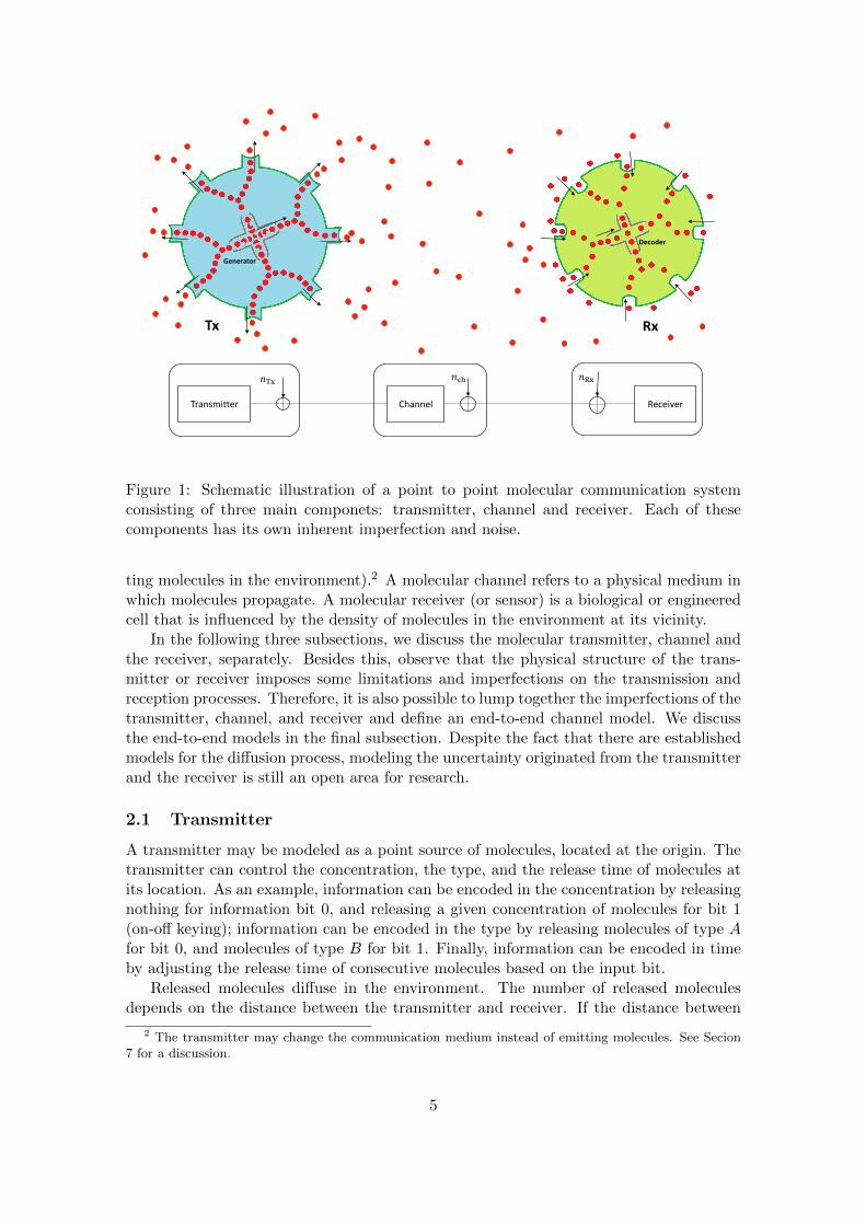
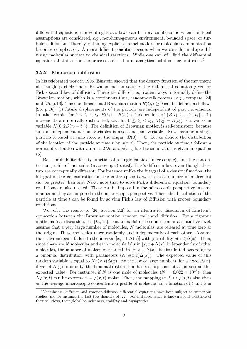
A point to point engineered communication system consists of a transmitter, a channel,and a receiver, as shown in Fig. 1. We employ this structure in our review of a molec-ular communication system. A molecular transmitter is a biological or engineered cellwhose actions influence the density of molecules in the environment (generally by emit-

1For instance, many cells move according to spatial differences in the concentration of certain chemicals(chemotaxis). In [16], an information theoretic criterion is proposed to model how cells find their migrationdirection from the imperfect information they obtain through chemical receptors on their surface.

4

Transmitter Channel Receiver

𝑛𝑛Tx 𝑛𝑛ch 𝑛𝑛Rx

Decoder

Rx

Generator

Tx

Figure 1: Schematic illustration of a point to point molecular communication systemconsisting of three main componets: transmitter, channel and receiver. Each of thesecomponents has its own inherent imperfection and noise.

ting molecules in the environment).2 A molecular channel refers to a physical medium inwhich molecules propagate. A molecular receiver (or sensor) is a biological or engineeredcell that is influenced by the density of molecules in the environment at its vicinity.

In the following three subsections, we discuss the molecular transmitter, channel andthe receiver, separately. Besides this, observe that the physical structure of the trans-mitter or receiver imposes some limitations and imperfections on the transmission andreception processes. Therefore, it is also possible to lump together the imperfections of thetransmitter, channel, and receiver and define an end-to-end channel model. We discussthe end-to-end models in the final subsection. Despite the fact that there are establishedmodels for the diffusion process, modeling the uncertainty originated from the transmitterand the receiver is still an open area for research.

2.1 Transmitter

A transmitter may be modeled as a point source of molecules, located at the origin. Thetransmitter can control the concentration, the type, and the release time of molecules atits location. As an example, information can be encoded in the concentration by releasingnothing for information bit 0, and releasing a given concentration of molecules for bit 1(on-off keying); information can be encoded in the type by releasing molecules of type Afor bit 0, and molecules of type B for bit 1. Finally, information can be encoded in timeby adjusting the release time of consecutive molecules based on the input bit.

Released molecules diffuse in the environment. The number of released moleculesdepends on the distance between the transmitter and receiver. If the distance between

2 The transmitter may change the communication medium instead of emitting molecules. See Secion7 for a discussion.

5

the transmitter and receiver is very small, individual molecules may be transmitted oneby one. If the distance is large, molecules get diluted in the environment before reachingthe receiver, and the transmitter may need to send considerably more molecules to ensurea viable communication line to the receiver.

Transmitter imperfection: In practice, the transmitter cannot perfectly control thenumber or the release time of the molecules. Furthermore, the molecule generation processof the transmitter can impose its own inherent constraints on the transmitter. To modelthese imperfections, one has to know the exact physical implementation of the transmitter.For instance, a physical description of a transmitter is detailed in [17, Section III.A]. In[18], different chemical reactions are considered for the emission of different symbols. In[5], the transmitter is assumed to have a reservoir of molecules, with an outlet whosesize is controlled by the transmitter. In other words, the transmitter may not control theexact number of molecules that exit the reservoir, but only the size of its outlet. Given thelarge number of molecules in the reservoir and a small probability of each exiting throughthe reservoir, the number of molecules exiting the outlet can be assumed to follow aPoisson distribution. Therefore, in this model, the number of released molecules from thetransmitter is a Poisson random variable, where its average or rate is determined by thetransmitter [5]. The Poisson model also arises in the following contexts:

• Poisson distribution models the number of escaped particles from a bounded domainwhen gates on the boundary of the domain open and close randomly, e.g. as in theescape of diffusing proteins from a corral in the plasma membrane [19, Sec. 3.6].Similarly, it arises in [20], wherein molecule release based on ion channels across thecell membrane is considered; the opening and closing of these channels are controlledby a gating parameter.

• It also arises when transmitter uses a colony of bacteria for molecule release. Eachreceptor on a bacterium releases a molecule with a probability that depends on theamount of provocation by the transmitter. If p is the release probability and N isthe total number of colony receptors, the number of released molecules follows abinomial distribution with parameters N and p. This can be approximated by aPoisson distribution if N is large and p is small.

Transmitter models: In this paper we focus on the following transmitter models:

• Timing transmitter : transmitter releases individual molecules one by one, at speci-fied time instances.

• Exact concentration transmitter: A time slotted transmission strategy is employed:time is divided into intervals of length Ts, with transmission occurring at the begin-ning of each time slot.3 The transmitter releases exactly Xi molecules (or Xi molesof molecule if the communication is very long range) at the beginning of the i-thtime slot, i.e., at time iTs.

• Poisson concentration transmitter: Again a time slotted transmission strategy isemployed. The number of released molecules from the transmitter at the beginningof the i-th time slot is a Poisson random variable with mean Xi.

3While this is a common assumption, it is possible to study communication rates via a continuous-time/amplitude model for the channel [21]. This is the only paper that we are aware of that studiesmutual information terms between input and output in continuous time domain.

6

2.2 Channel

To obtain a statistical model for a molecular channel, one has to specify the physicalmechanism of molecule transport between the transmitter and the receiver. The physicalmotion of molecules towards the receiver may be walk-based, flow-based, or diffusion-based [3]. In walk-based mechanisms, information molecules are encapsulated into acargo, which then by a motor protein, such as dynein and kinesin, are pushed toward thedestination through a pre-defined path, like microtubule tracks. It is an active propagationand requires chemical energy (ATP). In flow-based mechanisms, molecule propagationis influenced by an external flow, like propagation of hormones in the blood stream.Flow is a one-way phenomenon, which makes it unsuitable for a two-way communication.In contrast, in the diffusion-based transport, the molecules randomly propagate inall available directions via Brownian motion and have the most spontaneous motion.This results in a higher degree of uncertainty at the receiver, compared to the othermechanisms. The diffusion-based mechanism is completely passive and always availablewithout any energy cost or prior infrastructure, and is mostly suitable for highly dynamicand unpredictable environments. It is also possible to consider diffusion-based transportin the presence of a drift, resulting in a mixture of diffusion and flow based mechanisms.Most of the literature (as well as this paper) is focused on the diffusion-based transportmechanism.

Molecular diffusion can be studied from either microscopic or macroscopic points ofview. In a microscopic point of view, the focus is on the random movement of individualmolecules, known as the Brownian motion. In a macroscopic point of view, the focus is onthe overall behavior of an enormous number of molecules. Even though each molecule stillhas a random movement, but the total average behavior is characterized by a deterministicdifferential equation (due to the law of large numbers phenomenon); this deterministicdifferential equation is called the Fick’s law of diffusion. Historically, Fick proposed hismacroscopic law of diffusion in 1855, while the microscopic Brownian motion was studiedlater by Einstein in 1905; a full mathematical theory based on the theory of stochasticdifferential equations was developed only later in the 20th century.

2.2.1 Macroscopic diffusion

According to Fick’s first law of diffusion, diffusion flux goes from the region of highconcentration to the region of low concentration. Furthermore, the diffusion rate, denotedby J , is proportional to the concentration gradient. For simplicity of exposition, let usconsider one-dimensional diffusion 4. Then, Fick’s first law is:

J(x, t) = −D∂ρ(x, t)

∂x(1)

where J(x, t) and ρ(x, t) are respectively the diffusion flux, and molecule concentration(in molar) at location x at time t; D is the diffusion coefficient of the environment.

Now, assuming that there are no chemical reactions, drift velocity, or injection ofexternal molecules to the environment, we can use the mass conservation principle toconclude that

∂ρ(x, t)

∂t= −∂J(x, t)

∂x. (2)

4Equations describing the three-dimensional diffusion are similar to those describing the one-dimensional diffusion. Hence, to convey the intuition we start with a one-dimensional diffusion.

7

To intuitively understand the above equation, for a ∆x > 0, J(x, t)− J(x+ ∆x, t) showsthe entry rate of molecules from position x minus the exit rate of molecules from positionx + ∆x; if there is a mismatch between the entry and exit rates, the total number ofmolecules in the interval [x, x+ ∆x] changes at a rate equal to the difference of the entryand exit rates, i.e., at rate J(x, t)− J(x+ ∆x, t).

Equations (1) and (2) give us Fick’s second law of diffusion:

∂ρ(x, t)

∂t= D

∂2

∂x2ρ(x, t). (3)

If in addition to the diffusion process, we also have a molecule production rate, thechanges in molecule concentration will be both as a result of molecule production as wellas diffusion,

∂ρ(x, t)

∂t= −∂J(x, t)

∂x+ c(x, t). (4)

Here, for a given time t, c(x, t) denotes the density of molecule production rate at pointx, i.e., the number of molecules added to the environment in [x, x + dx] between time[t, t+ dt] is equal to c(x, t)dxdt. Then, we can write Fick’s second law as

∂ρ(x, t)

∂t= D

∂2

∂x2ρ(x, t) + c(x, t).

To solve this differential equation in an interval C = [a, b], it suffices to know the initialand boundary conditions: the initial density ρ(x, 0) at time zero for x ∈ C . The boundarycondition imposes some constraints on ρ(a, t) and ρ(b, t) as follows:

• Known values of ρ(x, t) at x = a, b for all t > 0: this corresponds to known con-centration on the boundaries. A special case of this is the zero boundary condition:ρ(a, t) = ρ(b, t) = 0; this corresponds to an absorbing boundary, i.e., molecules areabsorbed and removed from the environment upon hitting the boundary of C .

• Known values of ∂ρ(x,t)∂x at x = a, b for all t > 0: this corresponds to known diffusion

flux J(x, t) on the boundaries. A special case of this is the zero boundary condition:J(a, t) = J(b, t) = 0; this corresponds to a reflecting boundary, i.e., molecules thathit the boundary walls are reflected back into C .

When C = (−∞,∞) is the entire real line, the boundary can be placed as we takethe limits to infinity; for instance, one can solve the differential equation assuming thatρ(x, t) vanishes at infinity (as x becomes large). As an example, consider a transmitterthat is located at the origin (x = 0), and at time t = 0 suddenly releases one unit ofmolecules in the environment. In this case, the molecule production rate will be equal toc(x, t) = δ(x = 0)δ(t = 0). In response to this input, the output ρ(x, t) from equation (4)(assuming vanishing ρ(x, t) at infinity) is equal to the Green’s function:

ρ(x, t) =1[t > 0]

(4πDt)0.5e−

x2

4Dt . (5)

Observe that for a fixed t, ρ(x, t) as a function of x is the pdf of a Gaussian distributionwith variance 2Dt. This is no coincidence, and will become more transparent once weconsider the microscopic interpretation of the diffusion process.

If there is a drift, in addition to pure diffusion, influencing the molecules motion, themodified Fick’s laws may be employed to analyze the molecular channel. Solving the

8

differential equations representing Fick’s laws can be very cumbersome when non-idealassumptions are considered, e.g., non-homogeneous environment, bounded space, or tur-bulent diffusion. Thereby, obtaining explicit channel models for molecular communicationbecomes complicated. A more difficult condition occurs when we consider multiple dif-fusing molecules subject to chemical reactions. While one can still find the differentialequations that describe the process, a closed form analytical solution may not exist.5

2.2.2 Microscopic diffusion

In his celebrated work in 1905, Einstein showed that the density function of the movementof a single particle under Brownian motion satisfies the differential equation given byFick’s second law of diffusion. There are different equivalent ways to formally define theBrownian motion, which is a continuous time, random-walk process; e.g., compare [24]and [25, p.16]. The one-dimensional Brownian motion B(t), t ≥ 0 can be defined as follows[25, p.16]: (i) future displacements of the particle are independent of past movements.In other words, for 0 ≤ t1 < t2, B(t2) − B(t1) is independent of {B(t), t ∈ [0 : t1]}; (ii)increments are normally distributed, i.e., for 0 ≤ t1 < t2, B(t2) − B(t1) is a Gaussianvariable N (0, 2D(t2 − t1)). The definition of Brownian motion is self-consistent, becausesum of independent normal variables is also a normal variable. Now, assume a singleparticle released at time zero, at the origin: B(0) = 0. Let us denote the distributionof the location of the particle at time t by ρ(x, t). Then, the particle at time t follows anormal distribution with variance 2Dt, and ρ(x, t) has the same value as given in equation(5).

Both probability density function of a single particle (microscopic), and the concen-tration profile of molecules (macroscopic) satisfy Fick’s diffusion law, even though thesetwo are conceptually different. For instance unlike the integral of a density function, theintegral of the concentration on the entire space (i.e., the total number of molecules)can be greater than one. Next, note that to solve Fick’s differential equation, boundaryconditions are also needed. These can be imposed in the microscopic perspective in samemanner as they are imposed in the macroscopic perspective. Then, the distribution of theparticle at time t can be found by solving Fick’s law of diffusion with proper boundaryconditions.

We refer the reader to [26, Section 2.2] for an illustrative discussion of Einstein’sconnection between the Brownian motion random walk and diffusion. For a rigorousmathematical discussion, see [23, 24]. But to explain the connection at an intuitive level,assume that a very large number of molecules, N molecules, are released at time zero atthe origin. These molecules move randomly and independently of each other. Assumethat each molecule falls into the interval [x, x+∆(x)] with probability ρ(x, t)∆(x). Then,since there are N molecules and each molecule falls in [x, x+∆(x)] independently of othermolecules, the number of molecules that fall in [x, x + ∆(x)] is distributed according toa binomial distribution with parameters (N, ρ(x, t)∆(x)). The expected value of thisrandom variable is equal to Nρ(x, t)∆(x). By the law of large numbers, for a fixed ∆(x),if we let N go to infinity, the binomial distribution has a sharp concentration around thisexpected value. For instance, if N is one mole of molecules (N = 6.022 × 1023), thenNρ(x, t) can be expressed as ρ(x, t) molar. Then, the mapping (x, t) 7→ ρ(x, t) also givesus the average macroscopic concentration profile of molecules as a function of t and x in

5Nonetheless, diffusion and reaction-diffusion differential equations have been subject to numeriousstudies; see for instance the first two chapters of [22]. For instance, much is known about existence oftheir solutions, their global boundedness, stability and asymptotics.

9

terms of molar. On the other hand, we know that the macroscopic concentration satisfiesthe Fick’s laws of diffusion. As a result, ρ(x, t) satisfies the Fick’s laws of diffusion.

The above argument also provides a bridge between the macroscopic and microscopicperspectives: the macroscopic concentration is ρ(x, t) = Nρ(x, t), where the microscopicprobability density is ρ(x, t), and the number of molecules that fall into interval [x, x +∆(x)] is distributed according to a binomial distribution with parameters (N, ρ(x, t)∆(x)).This binomial distribution may be approximated by Gaussian or Poisson distributions[20, 27, 28, 29, 30, 31, 32]. In case of large Nρ(x, t)∆(x)(1 − ρ(x, t)∆(x)) (even forsmall ∆(x)), the binomial distribution can be approximated with a Normal distributionwith mean Nρ(x, t)∆(x) and variance Nρ(x, t)∆(x)(1− ρ(x, t)∆(x)) [33, p.80]. With theassumption that ρ(x, t)∆(x) is small, the variance Nρ(x, t)∆(x)(1 − ρ(x, t)∆(x)) can beapproximated with Nρ(x, t)∆(x). Then, the density of molecules, i.e., the number ofmolecules divided by ∆(x), follows a Normal distribution with mean Nρ(x, t) = ρ(x, t)and variance Nρ(x, t)∆(x)/∆(x)2 = ρ(x, t)/∆(x). To sum this up, if the macroscopicperspective on diffusion predicts a concentration ρ(x, t) molecules per volume, the actualconcentration of molecules per volume (in an interval ∆(x)) is a normal random variablewhose mean is ρ(x, t), and whose variance is ρ(x, t)/∆(x).

Example 1. Fick’s law of diffusion in terms of probability demonstrates how the distri-bution of the particle’s location at time t, denoted by ρ(x, t), changes over time. To showthe use of this fact, consider a transmitter located at the origin x = 0, and an absorbingreceiver located at x = d, at distance d from the transmitter. An absorbing receiver is par-ticularly important in molecular communication and the result of the following derivationis used elsewhere in the paper.

Assumed that a single molecule is released at time zero, therefore the initial distributionof the particle at t = 0 is ρ(x, 0) = δ(x). The molecule disappears upon hitting the receiver.Solving for Fick’s equation with the boundary conditions ρ(d, t) = 0 and limx→−∞ ρ(x, t) =0, we can obtain ρ(x, t)dx as the probability that the particle is located in [x, x+dx] at timet. We refer the reader to [26, Section 2.5] for the technique for solving Fick’s differential(4) with this boundary condition. Then, the probability that the particle has not hit thereceiver by time t is equal to ∫ d

x=−∞ρ(x, t)dx.

In other words, if T denotes the hitting time of a released particle with the absorbingreceiver, the distribution of T can be obtained as follows:

P[T ≥ t] =

∫ d

x=−∞ρ(x, t)dx.

In case of the diffusion equation given in (3) in a one-dimensional free homogeneousmedium with diffusion coefficient D, the first arrival time T at the receiver can be explicitlycalculated. First shown by Schrodinger in 1915, T has a Levy distribution [34]

fT (t) =

{ √λ

2πt3exp

(− λ

2t

), t > 0;

0, t ≤ 0.(6)

where λ = d2/2D. On the other hand, if the medium also has a velocity v towards thereceiver, the modified Fick’s law can be used to show that T follows an inverse Gaussian

10

distribution, IG(µ, λ) [35]:6:

fT (t) =

{ √λ

2πt3exp

(−λ(t−µ)2

2µ2t

), t > 0;

0, t ≤ 0.(7)

where

µ =d

v, and (8)

λ =d2

2D. (9)

Note that Levy is a heavy-tailed distribution (has infinite mean and variance), while IGhas an exponentially decreasing tail.

2.2.3 Statistical models of molecular channel

To construct a statistical model for a molecular channel, the microscopic and macroscopicviews of the diffusion should be appropriately utilized. On the transmitter side, if onlya few molecules are released, the microscopic perspective is relevant. However, if a largenumber of molecules are released by the transmitter, the macroscopic perspective becomesrelevant. On the other hand, in case of a single tiny molecular receiver, the microscopicbehavior of molecules around the receiver is of importance. As a result, if a large numberof molecules are released by the transmitter and the receiver is a single tiny nanomachine,we can employ the macroscopic view to compute the molecular concentration aroundthe receiver, but then switch to the microscopic view as discussed in Section 2.2.2, andconsider the actual number of molecules around the receiver. This is done explicitly laterin Section 2.4.

Finally, we comment that while in the above we restricted to one-dimensional diffusion,similar formulas hold for diffusion in three dimensions. While Fick’s law have extensionsfor nonhomogeneous environment with general boundary conditions, most existing worksstudy the simple case of an infinite medium in each direction, with no barrier or obstacleexcept the receiver surface.

2.3 Receiver

There are different models of the receiver in the literature:

• Sampling receiver: The simplest model for a receiver is a device that measures themacroscopic molecular concentration at a given point. The receiver’s observation isassumed not to affect the diffusion of the molecules, hence it imposes no boundaryconditions when solving Fick’s law of diffusion. The receiver may be assumed tosample the medium at certain given time instances.

• Transparent receiver: In this model, the receiver is a transparent sphere of volumeVR rather than a point, but still not affecting the diffusion of the molecules. Henceit imposes no boundary conditions when solving Fick’s law of diffusion. We mayassume that the receiver can perfectly count the number of molecules that fall into itssphere. This is the model used in [28] (see also [37]). The (microscopic) transparent

6A similar distribution holds for diffusion in a free three-dimensional environment [34, 36]

11

receiver differs from the (macroscopic) sampling receiver as follows: as discussedin Section 2.2.2, if a sampling receiver reads ρ(x, t), a transparent receiver reads anormal random variable whose mean is ρ(x, t), and whose variance is ρ(x, t)/VR.

• Absorbing receiver: The receiver absorbs any molecule that hits its surface. It keepsa count of the number of molecules that have hit it so far. Absorbing receivers implythe zero boundary condition when solving the Fick’s law of diffusion.

• Ligand or reactive receiver: This model is based on the receptors of natural cells thatare used in biological signaling pathways. It considers chemical kinetics of receptorslocated on the surface of the receiver. More specifically, it assumes that moleculesreaching the surface of the receiver may react and bind with the receptors on thesurface of the receiver and thereby initiate a chemical process inside the cell. Theliteratures generally consider cyclic adenosine monophosphate (cAMP) receptorsthat have a simple state space for each receptor: each receptor may be in thebound (B) or unbound (U) state with incoming molecules. Output at the receiveris the number of bound receptors. One important feature of a ligand receptor isits lingering effect, which is due to the fact that it takes some random time foreach receptor to be detached, after binding. The state transition of each receptordepends on the concentration of molecules around the receptor, and is governed bychemical equations [38].The most simplifying model is to take the statistical average of the number of boundreceptors to approximate the output, but then add a signal-dependent memorylessGaussian noise to represent all the modeling imperfections, i.e., the output can beexpressed as:

Z = αX +N (10)

for some constant α and Gaussian noise N [39]. In [40], a memoryless binomial(k, p)distribution is used for the number of bound receptors, where k is the total numberof receptors and the binding probability p is a function of concentration aroundthe receptors. In [21], the number of bound receptors is modeled by a Poisson dis-tribution whose parameter depends on the concentration of molecules around thereceiver.More accurate models of the ligand receptor use Markov chains to better representchemical equations at the receptors and the memory of the system. The state tran-sition probabilities of the Markov chain depend on the concentration of moleculesaround the receiver [40, 41]. More specifically, if there are k receptors on the surfaceof the receiver, we can denote the state by a vector in S = {B,U}k. The state attime instance i is also the output of the receiver, Yi = Si. The state transitionprobability p(si+1|si, xi) specifies the behavior of the ligand receptor [42]. The onlyassumption made about p(si+1|si, xi) in [41] is that when a receptor is in bound (B)state, the probability that it becomes unbound (U) does not depend on concentra-tion Xi.Finally, authors in [43] consider the boundary condition that a Ligand receptor im-poses (the boundary condition needed for solving the Fick’s law of diffusion). Theligand receptor is modeled by a partially absorbing boundary condition, in conjunc-tion with an active source of molecules. The partially absorbing boundary conditionreflects the fact that molecules hitting a receptor might not bind with the receptorand get reflected back into the environment (hence partially absorbing, partially

12

reflecting), and furthermore, a bound receptor might unbind and release a moleculeand hence an active source of molecule is included in the model.

2.4 End-to-end models

In this section, we review a number of existing end-to-end models derived by jointly con-sidering the transmitter, diffusion channel and receiver. It may be impossible to analyzeand model the end-to-end molecular channel independent from the release and receptionmechanisms at the transmitter and receiver, respectively. In other words, the release andthe reception mechanisms may have mutual effects with the molecular channel. Thereby,a joint analysis including the release, the transport, and the reception mechanisms isrequired.

Considering the three types of transmitter (timing transmitter, exact concentrationand Poisson concentration transmitter) and the four types of receiver (sampling receiver,transparent receiver, absorbing receiver, and ligand receiver), one can potentially identify3 × 4 = 12 combinations. However, some of the combinations are not meaningful (e.g.,the combination of a timing transmitter and a sampling receiver), and some are mathe-matically challenging (e.g. the combination of the ligand receiver with any of the threetransmitters). While transparent receiver [28, 29, 30], absorbing receiver [31], and ligandreceptors [44, 45] are all considered in the literature, only few of the possible transmit-ter/receiver combinations are studied. We shall review these combinations in the sequel.7

In describing an end-to-end model, it is useful to keep in mind the five types of noisethat may need to be accounted for [3]. The first type is the diffusion noise due to therandom propagation of individual molecules according to Brownian motion. We also havean environmental noise due to the degradation and/or reaction of molecules. There isalso a multiple transmitters noise from molecules diffused by unintended transmitters.Finally, there are two types of noise due to the physics of transceivers: the transmitteremission noise and receiver counting/reception noise.

In all of the models presented here, for simplicity and for being tractable, the trans-mitter is considered as a point source of molecules, located at the origin, and moleculesare assumed not to change while propagating in the medium and also not interact withthe transmitter. Motions of molecules do not influence each other and can be modeledby independent processes. Also, when using a concentration transmitter, a time-slottedcommunications with symbol period of Ts is assumed. The transmitter and receiver areassumed to be synchronized. Fick’s laws are employed in the models in different ways todetermine the parameters of the model.

2.4.1 Exact concentration transmitter with sampling or transparent receivers

The models that have an exact concentration transmitter with sampling or transparentreceivers are also called the linear models (also known as the deterministic models). Theyare described as follows:

Transmitter: The transmitter is assumed to be completely controlling the intensity ofmolecules at its location. The transmitter releases a large number of molecules (macro-scopic diffusion regime). The intensity should be non-negative.

Medium: Extending the Fick’s second law of diffusion (stated in (3)) to three-dimensionalspace [1] for a medium without any reaction and drift velocity, the concentration of

7See [46, 1] for two examples of models not discussed here.

13

molecules in the environment, denoted by ρ(~r, t), at location ~r and at time t is governedby

∂

∂tρ(~r, t) = D∇2ρ(~r, t) + c(~r, t), (11)

in which D is the diffusion coefficient of the transmitted molecule, and c(~r, t) is the densityof molecule production rate at point ~r at time t. Assuming that the transmitter is locatedat the origin, and at time t = 0 suddenly releases one unit of molecules in the environment,the density of the molecule production rate will be equal to c(~r, t) = δ(~r = 0)δ(t = 0).In response to this input, the output ρ(~r, t) from equation (11) is equal to the Green’sfunction:

h(~r, t) =1[t > 0]

(4πDt)1.5e−

‖r‖22

4Dt . (12)

Thus, (11) describes a linear time-invariant system, whose impulse response is given in(12).

The transmitter has a clock with frequency fs = 1/Ts, and instantaneously releasesXk molecules every Ts seconds, i.e., the density of production rate is the impulse train

c(~r, t) =∑k

Xkδ(~r = 0)δ(t− kTs),

then using the linearity of the diffusion system, the concentration of molecules at location~r at time t will be equal to

ρ(~r, t) =∑k

Xkh(~r, t− kTs). (13)

Receiver: The receiver has a clock too, with the same frequency fs (or possibly mul-tiples of it), using it to uniformly sample the medium at times jTs for j = 0, 1, 2, . . .. Wethen have

• (Sampling receiver): assume that the receiver is modeled by a point, located at~r∗, and is not affecting the diffusion medium. Furthermore, we assume that thereceiver can perfectly learn the macroscopic concentration of molecules at the timeof sampling. Then, we obtain Yj = ρ(~r∗, jTs). From (13),

Yj =∑k

Xkh(~r∗, jTs − kTs), j = 0, 1, 2, . . . (14)

=∑k

Xkpj−k, (15)

has a convolution form where pj = h(~r∗, jTs). From (12), it is clear that pj = 0 forj < 0, and thus the convolution can be written as:

Yj =∞∑k=0

pkXj−k. (16)

14

Noise process

Receiver

𝑵𝒌𝑿𝒌

𝒀𝒌

𝒑𝒌

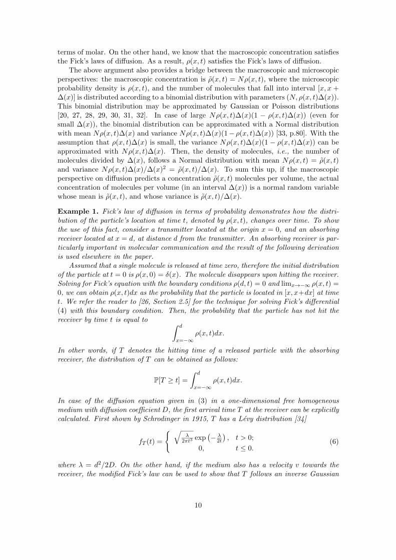
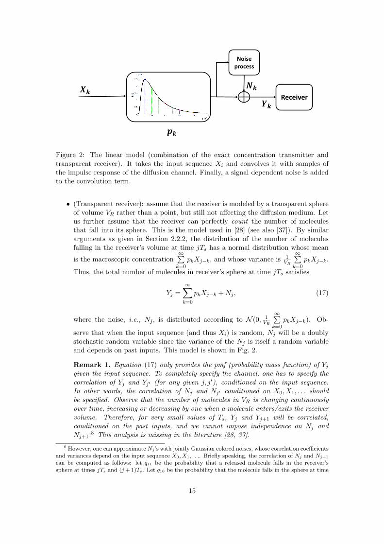
Figure 2: The linear model (combination of the exact concentration transmitter andtransparent receiver). It takes the input sequence Xi and convolves it with samples ofthe impulse response of the diffusion channel. Finally, a signal dependent noise is addedto the convolution term.

• (Transparent receiver): assume that the receiver is modeled by a transparent sphereof volume VR rather than a point, but still not affecting the diffusion medium. Letus further assume that the receiver can perfectly count the number of moleculesthat fall into its sphere. This is the model used in [28] (see also [37]). By similararguments as given in Section 2.2.2, the distribution of the number of moleculesfalling in the receiver’s volume at time jTs has a normal distribution whose mean

is the macroscopic concentration∞∑k=0

pkXj−k, and whose variance is 1VR

∞∑k=0

pkXj−k.

Thus, the total number of molecules in receiver’s sphere at time jTs satisfies

Yj =∞∑k=0

pkXj−k +Nj , (17)

where the noise, i.e., Nj , is distributed according to N (0, 1VR

∞∑k=0

pkXj−k). Ob-

serve that when the input sequence (and thus Xi) is random, Nj will be a doublystochastic random variable since the variance of the Nj is itself a random variableand depends on past inputs. This model is shown in Fig. 2.

Remark 1. Equation (17) only provides the pmf (probability mass function) of Yjgiven the input sequence. To completely specify the channel, one has to specify thecorrelation of Yj and Yj′ (for any given j, j′), conditioned on the input sequence.In other words, the correlation of Nj and Nj′ conditioned on X0, X1, . . . shouldbe specified. Observe that the number of molecules in VR is changing continuouslyover time, increasing or decreasing by one when a molecule enters/exits the receivervolume. Therefore, for very small values of Ts, Yj and Yj+1 will be correlated,conditioned on the past inputs, and we cannot impose independence on Nj andNj+1.8 This analysis is missing in the literature [28, 37].

8 However, one can approximateNj ’s with jointly Gaussian colored noises, whose correlation coefficientsand variances depend on the input sequence X0, X1, . . .. Briefly speaking, the correlation of Nj and Nj+1

can be computed as follows: let q11 be the probability that a released molecule falls in the receiver’ssphere at times jTs and (j+ 1)Ts. Let q10 be the probability that the molecule falls in the sphere at time

15

From the five types of noise mentioned in Section 2.4, none of them was considered inthe model given for the sampler receiver. And only diffusion noise was considered in themodel given for the transparent receiver. It is possible to modify the model to considerother noises in the model. For instance consider the case in which the receiver has a smallvolume VR and imperfectly counts the number of molecules that fall into that area. Thisincurs a particle counting noise in addition to the diffusion noise.

2.4.2 Poisson concentration transmitter with absorbing receiver

Poisson concentration transmitter with absorbing receiver is also called the Poisson Model.Transmitter: The transmitter chooses a rate Xi ≥ 0 at time slot i. The number of

released molecules in the beginning of the i-th time-slot is a Poisson random variable,where its average or rate, is Xi. As a result, the density of production rate is the impulsetrain

c(~r, t) =∑k

Skδ(~r = 0)δ(t− kTs),

where Sk ∼ Poisson(Xi) is the number of released molecules at time kTs by a transmitterlocated at the origin. Random variable Sk is a doubly stochastic random variable (aPoisson distribution whose parameter is the random variable Xi).

Medium and receiver: Each released molecule is absorbed upon hitting the receiver.Let pk, k = 0, 1, 2, . . ., denote the probability that a released molecule at the currentslot hits the receiver in the next k-th time slot. The values of pk’s depend on the com-munication medium and in general can be derived from Fick’s diffusion law. For a one-dimensional motion, the distribution of the hitting time T was found in Example 1. Then,the hitting probability can be computed as follows:

pk =

∫ (k+1)Ts

kTs

fT (t). (18)

Distribution of the first hitting time (and the values of pk) for a non-uniform mediumthat is arbitrarily filled with barrier or obstacles may be found by numerically solving theFick’s equations.

Generally, the signal is decoded at the receiver based on the total number of moleculesreceived during the individual time slots. In a time slot, three sources contribute to thereceived molecules: (i) molecules due to the transmission in the current time slot, (ii) theresidue molecules due to the transmission in the earlier time slots known as the interferencesignal, and (iii) noise molecules, modeled within a slot of duration Ts as a Poisson randomvariable with parameter λ0Ts. Based on the thinning property of Poisson distribution,the number of received molecules in the time slot i, denoted by Yi, is as follows [5]:

Yi ∼ Poisson

(λ0Ts +

i∑k=0

pkXi−k

)= Poisson(Ii + p0Xi) (19)

jTs, but does not fall at time (j + 1)Ts; q01 is defined reversely and q00 is the probability that moleculedoes not fall in either of times jTs or (j + 1)Ts. If we release a deterministic number x of molecules attime zero, we can define a multinomial distribution Z00, Z01, Z10, Z11 with parameters x and probabilities(q00, q01, q10, q11). Then Yj = Z10 + Z11 and Yj+1 = Z01 + Z11 are the number of molecules receivedin times slots jTs and (j + 1)Ts respectively. If q01, q10, q11 are small, we can approximate Z10, Z01 andZ11 by independent Gaussian distributions. Thus, Yj and Yj+1 will be jointly (colored) Gaussian randomvariables when we transmit x molecules at time zero.

16

where Ii is the sum of interference and noise at time i. The above equation statesp(yi|x[0:i]), which together with

p(y[0:n]|x[0:n]) =n∏i=1

p(yi|x[0:i]) (20)

describes the Poisson channel completely. Equation (20) is proved using the thinningproperty of Poisson distribution in [5].

From the five types of noise mentioned in Section 2.4, transmitter noise, diffusion noiseand multiple transmitters noise are taken into account. Transmitter noise is reflected inthe fact that the number of molecules exiting the transmitter cannot be exactly controlled;diffusion noise is considered because the model is based on microscopic Brownian motion,and finally multiple transmitters and background noise is considered by the λ0Ts term.

2.4.3 Timing transmitter with absorbing receiver

Timing transmitter with absorbing receiver leads to what is known as the Timing Modelfor MC.

Transmitter: The transmitter is assumed to be completely controlling the releasetime of molecules one by one at its location. Information is coded in the release time ofindividual molecules [47].

Medium and receiver: The released molecules randomly propagate according to theBrownian motion. Each molecule may arrive at the receiver after a (random) delay, or maynever arrive at the receiver.9 Molecules do not arrive if the Brownian motion is transient,or the molecules fade away in the environment. Since we consider an absorbing receiver,each molecule hits the receiver at most once. Despite the uncertainty in the arrival timesof the molecules, these arrival times are statistically correlated with their release time,and this correlation can be used for information transmission. In this context, informationtransmission capacity may be measured by bits per unit of time [34, 48], bits per molecule[48], or bits per joule [49] for a given production rate of molecules.

Timing channel models generally ignore the existence of noise molecules, i.e., moleculesof the same type in the environment that are not diffused by the transmitter. Noisemolecules are likely to complicate the problem significantly. From the five types of noisementioned in Section 2.4, only diffusion noise is taken into account.10

Assuming that a molecule is released at time X, the arrival time is equal to Z = X+T ,where T is the transmission delay. Because molecules are absorbed upon hitting thereceiver, the distribution of T is that of a first arrival time. For a one-dimensional motionwith variance σ2, a positive drift v > 0 and travel distance d, T will follow an inverseGaussian distribution IG(µ, λ) given in equation (7). When there is no drift v = 0, Tfollows the Levy distribution given in equation (6).

2.4.4 Ligand receiver with simplification on the transmitter side

These models focus on the physical complexity of the receiver and simplify the channelnoise, with the goal of understanding fundamental limits imposed by the receiver alone.

9The lifetime of a molecule may be modeled by Weibull distribution [50] which is a widely used lifetimedistribution, or bounded by a hard threshold [34].

10Some variations of the timing model consider a maximum lifetime for molecules; hence a form ofdegradation noise is considered as well.

17

Transmitter and medium: It is assumed that the concentration of molecules aroundthe receiver at time slot i is a function of transmission in that time slot, i.e., f(Xi) forsome known function f(·).

Receiver: A receiver with cAMP receptors that was described in Section 2.3 is as-sumed.

3 Literature review: concentration transmitter

One of the popular signaling methods in molecular communication uses the molecules’concentration to encode the information. In this setup, the transmitter encodes informa-tion into the concentration of released molecules. The released molecules follow a diffusionprocess through the channel to reach the receiver. As discussed in Section 2, the temporaland spatial concentration of molecules can be derived by the Fick’s second law of diffusionwhich results in a distance-time dependent impulse response.

There are several works in the literature on the concentration signaling, many of whichclaim complete characterizations of channel capacity, leaving the general impression tounfamiliar readers that the capacity of molecular channels is solved. However, once we goinside the papers we see that the capacity calculations are mostly done after simplificationsin terms of the channel memory. Simplification and approximation have the advantageof leading to explicit expressions. But one needs to also address how the derived boundsrelate to the actual channel capacity without any simplifications, by specifying whetherthey are lower or upper bounds to the actual capacity.

Having said that, in principle, the capacity of concentration signaling, consideringthe transmitter-receiver limitations and the intersymbol interference (ISI) effect of thechannel is not an open problem, under some reasonable physical assumptions. As pointedout in [51], we may model the diffusion channel (possibly with drift in a non-uniformmedium) as a state dependent channel. Here the state models the number or density ofmolecules across the environment; we can divide the space into very small cells and keepthe number of molecules in the cells as the current state of the medium. Part of thestate can also model the bound/unbound state receptors on the surface of the receiver.Then, observe that the resulting state-dependent channel is indecomposable [52, p. 105]as the initial state diffuses away over time under reasonable physical constraints on themedium. Thus, one can characterize the capacity in a computable form [52]. However,the state space is very large and capacity characterization is in finite-letter form, makingit prohibitively hard to compute and thus of little practical value.11

In the following, we describe some approaches that exist in the literature.

3.1 Linear Model

The goal is to study the capacity of the channel

Yj =∞∑k=0

pkXj−k +Nj , (21)

11From an information theoretic perspective, a characterization of the capacity region is called com-putable if there exists an algorithm (constructed based on the characterization) that gets an approximationlevel ε as its inputs and halts in finite time and produces a curve within ε distance of the capacity region.There is no restriction on the time that takes for the algorithm to halt.

18

where the noise, i.e., Nj , is distributed according to N (0, 1VR

∞∑k=0

pkXj−k). The input

constraint consists of non-negativity of input concentration Xi ≥ 0, and possibly maxi-mum and average concentration constraints: |Xi| ≤ A and

∑ni=1Xi/n ≤ Es. To study

the capacity of this channel, one has to specify the joint distribution of N1, N2, . . . condi-tioned on the entire input sequence as discussed in Remark 1. Even with the assumptionof conditional independence of Nj (which is justified when Ts is large), as far as we areaware, the capacity of the above channel has not been studied. If the variance of Nj

were some constant σ2 and channel inputs were allowed to become negative, the problemwould have reduced to the classical Gaussian ISI channel that has been subject to manystudies, starting from the work by Hirt and Massey in [53]. Nonetheless, much of theclassical ideas clearly carry over from the classical ISI channels. For instance, one canfind bounds on capacity using the ideas of using i.i.d. input distribution [54]. Also, whenthe number of terms in the linear expansion (21) is finite (pk > 0 for large enough k), wecan find computable finite-letter expressions for the capacity using the ideas presentedlater in Section 3.2.

The existing literature on the linear model simplify the problem by discarding thechannel memory. In this approach, the molecular channel is approximated by a memory-less channel (in many cases, a channel with binary input alphabet) whose capacity can bereadily found by maximizing the input-output mutual information (e.g., see [55, 56, 39]).Thus, while these papers might be valuable in the context of modeling, they are not excit-ing to information theorists. These approaches do not genuinely consider a channel withmemory, as the interference from past inputs (ISI) is either ignored, or averaged and putinto the transition probabilities of a memoryless channel.12

The binary input restriction may be justified by the fact that nano nodes should besimple, and one of the simplest transmission strategies is the On-Off Keying modulationin which no molecule is transmitted for information bit 0 and Amax concentration isreleased for information bit 1. While On-Off keying simplifies the transmitter’s design,receiver’s design can be simplified to a simple threshold decoder by adopting transmissionmodulation schemes that reduce or mitigate the ISI. Thus, channel simplifications andrestriction to certain modulation schemes may not be unjustified as it may appear in firstglance.

Finally, there are also some works based on the quorum sensing property of bacterialcolonies [12, 57] that also consider a memoryless channel, but with an input-dependentnoise. Even though we obtained the linear model for an exact concentration transmitter,the same end-to-end model applies to the works based on quorum sensing.13 In theseworks, the transmitter and receiver employ bacterial colonies. The collective behaviorof the bacteria in response to stimuli is exploited for transmission and reception. Thecolony on the transmitter side, in the steady state, senses the concentration of a specialmolecule type and in response produces and releases another type of molecules. The re-leased molecules propagate in the medium based on diffusion equations, which has beenconsidered in the steady state. Similar to the transmitter, the receiver senses the concen-tration based on the quorum sensing property. All limitations, i.e., noises, are modeledwith an additive Gaussian noise with input-dependent variance (still a memoryless chan-

12A variation of this approach is proposed in [60] by considering two binary channel, one of which occursdepending on the last transmitted symbol.

13By ignoring ISI and considering Nj as the transmitter or the receiver noise in (21), the linear modelreduces to the model of these works (which was obtained by using a Gaussian approximation for thebinomial distribution) if the dependency between the transmitter and receiver noises is ignored.

19

nel), and no ISI terms are considered. In the same scenario of biological nodes consistingof bacteria, the relaying is studied in [58, 59], where the relay exploits its quorum sensingproperty to apply the sense and forward scheme (which is parallel to the amplify andforward scheme in the classic communication).

3.2 Poisson Model

The goal is to compute the capacity of the LTI-Poisson channel

Yi ∼ Poisson

λ0Ts +i∑

j=0

pjXi−j

(22)

under average and maximum intensity cost constraints. More specifically, the followingconstraints on the input codewords of length n are assumed: Xi ≥ 0, average inputconstraint

∑ni=1Xi/n ≤ Es and a constraint on the maximum value of Xi, Xi ≤ A.

The summation∑i

j=0 pjXi−j is the convolution of the sequence (X0, X1, . . .) with thesequence p = (p0, p1, p2, . . .). This makes the Yi as the output of a channel consisting of acascade of an LTI system (with impulse response p) and a memoryless Poisson channel,called an LTI-Poisson channel in [51]. This model can be understood as a generalizationof the classical memoryless Poisson channel. Therefore, the LTI-Poisson model relates totwo bodies of literature in information theory: networks with memory and memorylessPoisson channels. A common point in both literatures is an attempt to find easy-to-compute expressions for the capacity (e.g. see [61, 62]).

The capacity for the channel given in equation (22) is claimed to have been solved in[63, p. 9, eqn. (40)]. However, in the proof on page 10 of [63], after equation (50), it isclaimed that Yi’s are i.i.d. and H(Y n) is expanded as

∑ni=1H(Yi). But Yi’s are correlated

in general because they depend on the input sequence Xi.The capacity for this channel has been characterized in [51] under the assumption

that molecules injected into the environment will disappear after k time-slots, for somelarge enough k. Thus, pi = 0 for i > k. This allows one to write that

Yi ∼ Poisson

λ0Ts +

k∑j=0

pjXi−j

. (23)

In particular, p(yi|x[0:i]) = p(yi|x[i−k:i]), and from equation (20)

p(y0:n|x1:n) =

n∏i=0

p(yi|xi:i−k). (24)

The factorization given in equation (24) allows for a multi-letter, albeit computable char-acterization of the capacity region. Factorization of the type given by (24) was firstexploited by Verdu for MAC channels [64]. Verdu’s motivation for defining this class ofnetworks was to study linear ISI channels. The intuitive reason that factorization of (24)is useful is that one can set or reset the channel state using any k consecutive inputs (asthe channel remembers only the last k inputs)[51].

In [51], the capacity of the original channel (with memory) is sandwiched betweenthe capacities of two memoryless channels, i.e., two memoryless channels are given whosecapacities bound the desired capacity from below and above. The upper and lower bounds

20

can be made arbitrarily close to each other, resulting in a computable characterization ofthe capacity region.

For the lower bound, a natural number r is chosen. Then time is partitioned into blocksof size k+r, i.e. one block for time instances 1 to k+r, one block for time instances k+r+1to 2(k + r), etc. Then, the channel is depreciated by deleting output Yi’s for the first ktime instances of each block. In other words, the new channel after deletion has inputsX1, X2, · · · and outputs Yk+1, Yk+2, · · · , Yk+r and then Y2k+r+1, Y2k+r+1, · · · , Y2k+2r, etc.Because the outputs in each block depend only on inputs in the same block, the resultingchannel is block memoryless and its capacity lies below the capacity of original channel.

For the upper bound, a natural number r is chosen. Then time is partitioned intoblocks of size r; in other words, first block covers time instances 1 to r, second block coverstime instances r + 1 to 2r, etc. The channel is enhanced by allowing the transmitter toarbitrarily “reset” the memory of the channel (k last inputs) at the beginning of eachblock (without any regard to its actual last k inputs). The new channel has a highercapacity than the original channel, since the memory content specified by the transmitterat the beginning of each block can simply be the actual state that the system would havebeen in, if transmitter did not have the option of changing the memory content of thechannel. Furthermore, the new channel is block memoryless and its capacity lies abovethe capacity of original channel.

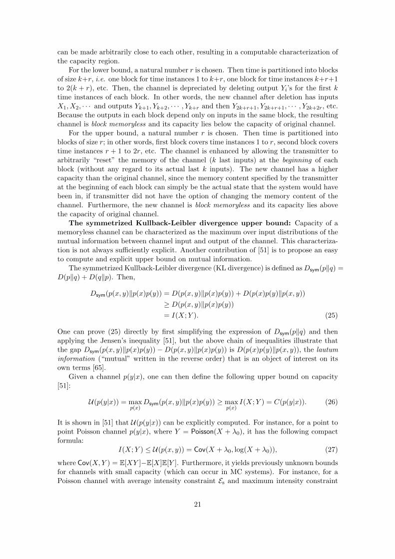
The symmetrized Kullback-Leibler divergence upper bound: Capacity of amemoryless channel can be characterized as the maximum over input distributions of themutual information between channel input and output of the channel. This characteriza-tion is not always sufficiently explicit. Another contribution of [51] is to propose an easyto compute and explicit upper bound on mutual information.

The symmetrized Kullback-Leibler divergence (KL divergence) is defined asDsym(p‖q) =D(p‖q) +D(q‖p). Then,

Dsym(p(x, y)‖p(x)p(y)) = D(p(x, y)‖p(x)p(y)) +D(p(x)p(y)‖p(x, y))

≥ D(p(x, y)‖p(x)p(y))

= I(X;Y ). (25)

One can prove (25) directly by first simplifying the expression of Dsym(p‖q) and thenapplying the Jensen’s inequality [51], but the above chain of inequalities illustrate thatthe gap Dsym(p(x, y)‖p(x)p(y))−D(p(x, y)‖p(x)p(y)) is D(p(x)p(y)‖p(x, y)), the lautuminformation (“mutual” written in the reverse order) that is an object of interest on itsown terms [65].

Given a channel p(y|x), one can then define the following upper bound on capacity[51]:

U(p(y|x)) = maxp(x)

Dsym(p(x, y)‖p(x)p(y)) ≥ maxp(x)

I(X;Y ) = C(p(y|x)). (26)

It is shown in [51] that U(p(y|x)) can be explicitly computed. For instance, for a point topoint Poisson channel p(y|x), where Y = Poisson(X + λ0), it has the following compactformula:

I(X;Y ) ≤ U(p(x, y)) = Cov(X + λ0, log(X + λ0)), (27)

where Cov(X,Y ) = E[XY ]−E[X]E[Y ]. Furthermore, it yields previously unknown boundsfor channels with small capacity (which can occur in MC systems). For instance, for aPoisson channel with average intensity constraint Es and maximum intensity constraint

21

A, this bound is calculated as:

UPoisson(p(y|x)

):= max

p(x):E[X]=Es, 0≤X≤A

U(p(x, y)) =

EsA (A− Es) log

(Aλ0

+ 1), Es < A/2

A4 log

(Aλ0

+ 1), Es ≥ A/2.

For previous works on Poisson channel and other techniques for bounding mutual infor-mation, see [61, 62].

3.3 Other models

Authors in [32] consider a combination of an exact concentration transmitter and anabsorber receiver. The exact concentration transmitter can send 0 ≤ Xi ≤ N moleculesat the beginning of each time slot. The receiver counts the number of absorbed moleculesin each time slot. Consider the hitting probabilities {pk} of the absorbing receiver inequation (18). Then, each of the X0 molecules released in the first time slot arrive inthe k-th time slot with probability pk. Thus, the total number of molecules that arereleased in time slot 0 and arrive in the k-th time slot follows a binomial distribution withparameters (X0, pk). Since we have a transmission at the beginning of each time slot, thetotal number of molecules received at the time slot k is the sum of independent binomialrandom variables corresponding to transmissions from time slots k, k− 1, k− 2, etc. Thesum of independent binomial variables does not have a nice analytical form. The moreserious difficulty is the correlation that arises between outputs at different time-slots.14

There are only some approximation techniques for handling dependencies that arise insuch balls and bins problems; see for instance [66, Section 5.4]. Authors in [32] simplifythe problem by assuming that pk = 0 for k ≥ 2. Furthermore, they handle the correlationby assuming an i.i.d. input distribution when evaluating the n-letter mutual informationform of the channel capacity. We will review the idea of evaluating the n-letter mutualinformation by assuming an i.i.d. distribution in relation to a different problem in detailin Section 4.

A different model for the diffusion medium is considered in [67]. The transmitter is stillan exact concentration transmitter, but instead of using the linear model and Fick’s lawto evaluate the concentration at the receiver, the authors assume that the concentrationat the receiver can be at either of the two “low” or “high” concentration states. Inother words, the communication medium is modeled with a two-state Markov chain, withlow and high states, which indicate the “overall” intensity of residual molecules in theenvironment due to the past transmissions (high ISI or low ISI). By using the On-OffKeying scheme and assuming memory of depth one, an achievable rate is derived in [67].

4 Literature review: timing transmitter

The capacity of molecular timing channels has been the subject of several studies. Theseworks appeal to information theorists because they exploit serious information theoretictools and are mathematically rigorous. While it is not possible to reproduce the entire

14This is the main advantage of the Poisson concentration transmitter over the exact concentrationtransmitter in the presence of an absorbing receiver (see equation (24)). The linear model (that uses atransparent receiver) also has a similar disadvantage as discussed in Remark 1.

22

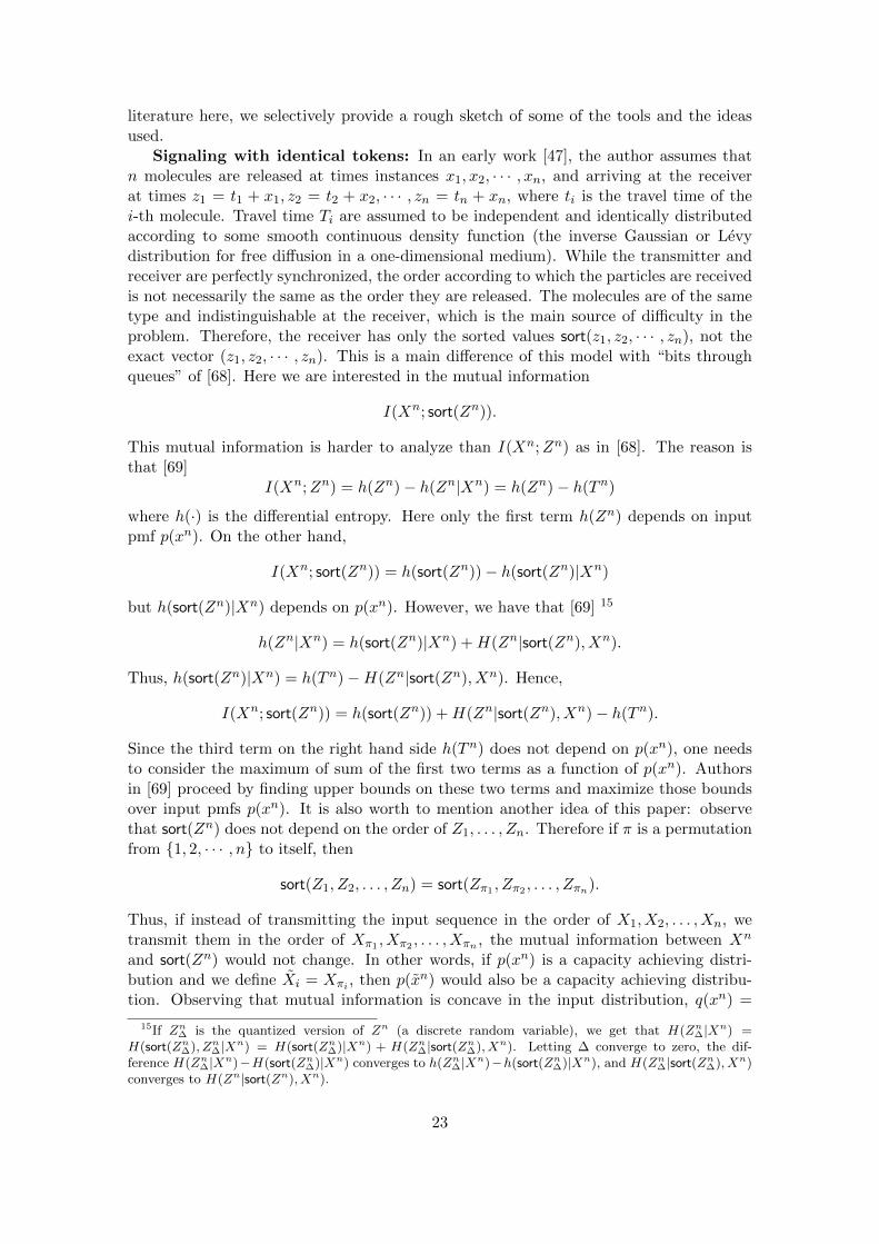
literature here, we selectively provide a rough sketch of some of the tools and the ideasused.

Signaling with identical tokens: In an early work [47], the author assumes thatn molecules are released at times instances x1, x2, · · · , xn, and arriving at the receiverat times z1 = t1 + x1, z2 = t2 + x2, · · · , zn = tn + xn, where ti is the travel time of thei-th molecule. Travel time Ti are assumed to be independent and identically distributedaccording to some smooth continuous density function (the inverse Gaussian or Levydistribution for free diffusion in a one-dimensional medium). While the transmitter andreceiver are perfectly synchronized, the order according to which the particles are receivedis not necessarily the same as the order they are released. The molecules are of the sametype and indistinguishable at the receiver, which is the main source of difficulty in theproblem. Therefore, the receiver has only the sorted values sort(z1, z2, · · · , zn), not theexact vector (z1, z2, · · · , zn). This is a main difference of this model with “bits throughqueues” of [68]. Here we are interested in the mutual information

I(Xn; sort(Zn)).

This mutual information is harder to analyze than I(Xn;Zn) as in [68]. The reason isthat [69]

I(Xn;Zn) = h(Zn)− h(Zn|Xn) = h(Zn)− h(Tn)

where h(·) is the differential entropy. Here only the first term h(Zn) depends on inputpmf p(xn). On the other hand,

I(Xn; sort(Zn)) = h(sort(Zn))− h(sort(Zn)|Xn)

but h(sort(Zn)|Xn) depends on p(xn). However, we have that [69] 15

h(Zn|Xn) = h(sort(Zn)|Xn) +H(Zn|sort(Zn), Xn).

Thus, h(sort(Zn)|Xn) = h(Tn)−H(Zn|sort(Zn), Xn). Hence,

I(Xn; sort(Zn)) = h(sort(Zn)) +H(Zn|sort(Zn), Xn)− h(Tn).

Since the third term on the right hand side h(Tn) does not depend on p(xn), one needsto consider the maximum of sum of the first two terms as a function of p(xn). Authorsin [69] proceed by finding upper bounds on these two terms and maximize those boundsover input pmfs p(xn). It is also worth to mention another idea of this paper: observethat sort(Zn) does not depend on the order of Z1, . . . , Zn. Therefore if π is a permutationfrom {1, 2, · · · , n} to itself, then

sort(Z1, Z2, . . . , Zn) = sort(Zπ1 , Zπ2 , . . . , Zπn).

Thus, if instead of transmitting the input sequence in the order of X1, X2, . . . , Xn, wetransmit them in the order of Xπ1 , Xπ2 , . . . , Xπn , the mutual information between Xn

and sort(Zn) would not change. In other words, if p(xn) is a capacity achieving distri-bution and we define Xi = Xπi , then p(xn) would also be a capacity achieving distribu-tion. Observing that mutual information is concave in the input distribution, q(xn) =

15If Zn∆ is the quantized version of Zn (a discrete random variable), we get that H(Zn

∆|Xn) =H(sort(Zn

∆), Zn∆|Xn) = H(sort(Zn

∆)|Xn) + H(Zn∆|sort(Zn

∆), Xn). Letting ∆ converge to zero, the dif-ference H(Zn

∆|Xn)−H(sort(Zn∆)|Xn) converges to h(Zn

∆|Xn)−h(sort(Zn∆)|Xn), and H(Zn

∆|sort(Zn∆), Xn)

converges to H(Zn|sort(Zn), Xn).

23

12pXn(xn) + 1

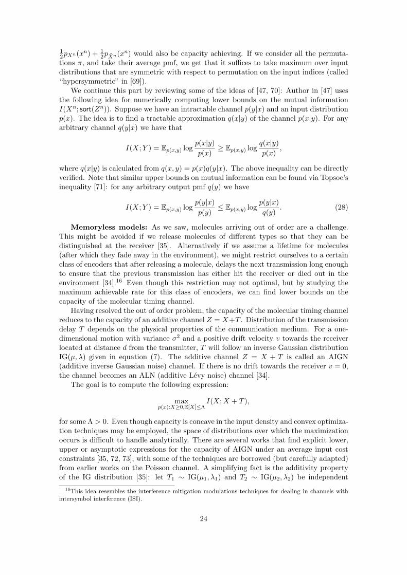
2pXn(xn) would also be capacity achieving. If we consider all the permuta-tions π, and take their average pmf, we get that it suffices to take maximum over inputdistributions that are symmetric with respect to permutation on the input indices (called“hypersymmetric” in [69]).

We continue this part by reviewing some of the ideas of [47, 70]: Author in [47] usesthe following idea for numerically computing lower bounds on the mutual informationI(Xn; sort(Zn)). Suppose we have an intractable channel p(y|x) and an input distributionp(x). The idea is to find a tractable approximation q(x|y) of the channel p(x|y). For anyarbitrary channel q(y|x) we have that

I(X;Y ) = Ep(x,y) logp(x|y)

p(x)≥ Ep(x,y) log

q(x|y)

p(x),

where q(x|y) is calculated from q(x, y) = p(x)q(y|x). The above inequality can be directlyverified. Note that similar upper bounds on mutual information can be found via Topsoe’sinequality [71]: for any arbitrary output pmf q(y) we have

I(X;Y ) = Ep(x,y) logp(y|x)

p(y)≤ Ep(x,y) log

p(y|x)

q(y). (28)

Memoryless models: As we saw, molecules arriving out of order are a challenge.This might be avoided if we release molecules of different types so that they can bedistinguished at the receiver [35]. Alternatively if we assume a lifetime for molecules(after which they fade away in the environment), we might restrict ourselves to a certainclass of encoders that after releasing a molecule, delays the next transmission long enoughto ensure that the previous transmission has either hit the receiver or died out in theenvironment [34].16 Even though this restriction may not optimal, but by studying themaximum achievable rate for this class of encoders, we can find lower bounds on thecapacity of the molecular timing channel.

Having resolved the out of order problem, the capacity of the molecular timing channelreduces to the capacity of an additive channel Z = X+T . Distribution of the transmissiondelay T depends on the physical properties of the communication medium. For a one-dimensional motion with variance σ2 and a positive drift velocity v towards the receiverlocated at distance d from the transmitter, T will follow an inverse Gaussian distributionIG(µ, λ) given in equation (7). The additive channel Z = X + T is called an AIGN(additive inverse Gaussian noise) channel. If there is no drift towards the receiver v = 0,the channel becomes an ALN (additive Levy noise) channel [34].

The goal is to compute the following expression:

maxp(x):X≥0,E[X]≤Λ

I(X;X + T ),

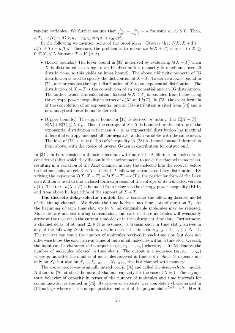
for some Λ > 0. Even though capacity is concave in the input density and convex optimiza-tion techniques may be employed, the space of distributions over which the maximizationoccurs is difficult to handle analytically. There are several works that find explicit lower,upper or asymptotic expressions for the capacity of AIGN under an average input costconstraints [35, 72, 73], with some of the techniques are borrowed (but carefully adapted)from earlier works on the Poisson channel. A simplifying fact is the additivity propertyof the IG distribution [35]: let T1 ∼ IG(µ1, λ1) and T2 ∼ IG(µ2, λ2) be independent

16This idea resembles the interference mitigation modulations techniques for dealing in channels withintersymbol interference (ISI).

24

random variables. We further assume that λ1

c1µ21

= λ2

c2µ22

= κ for some c1, c2 > 0. Then,

c1T1 + c2T2 ∼ IG(c1µ1 + c2µ2, κ(c1µ1 + c2µ2)2).In the following we mention some of the proof ideas. Observe that I(X;X + T ) =

h(X + T ) − h(T ). Therefore, the problem is to maximize h(X + T ) subject to X ≥0,E[X] ≤ Λ for some T ∼ IG(µ, λ).

• (Lower bounds:) The lower bound in [35] is derived by evaluating h(X + T ) whenX is distributed according to an IG distribution (capacity is maximum over alldistributions, so this yields an inner bound). The above additivity property of IGdistribution is used to specify the distribution of X+T . To derive a lower bound in[72], author chooses the input distribution of X to an exponential distribution. Thedistribution of X + T is the convolution of an exponential and an IG distribution.The author avoids this calculation. Instead h(X + T ) is bounded from below usingthe entropy power inequality in terms of h(X) and h(T ). In [73], the exact formulaof the convolution of an exponential and an IG distribution is cited from [74] and anew analytical lower bound is derived.

• (Upper bounds:) The upper bound in [35] is derived by noting that E[X + T ] =E[X] +E[T ] ≤ Λ +µ. Thus, the entropy of X + T is bounded by the entropy of theexponential distribution with mean Λ + µ, as exponential distribution has maximaldifferential entropy amongst all non-negative random variables with the same mean.The idea of [73] is to use Topsoe’s inequality in (28) to bound mutual informationfrom above, with the choice of inverse Gaussian distribution for output pmf.

In [34], authors consider a diffusion medium with no drift. A lifetime for molecules isconsidered (after which they die out in the environment) to make the channel memoryless,resulting in a variation of the ALN channel: in case the molecule hits the receiver beforeits lifetime ends, we get Z = X + T , with T following a truncated Levy distribution. Bywriting the expansion I(X;X + T ) = h(X + T )− h(T ), the particular form of the Levydistribution is used to find a closed form expression of the entropy of its truncated versionh(T ). The term h(X+T ) is bounded from below via the entropy power inequality (EPI),and from above by logarithm of the support of X + T .

The discrete delay-selector model: Let us consider the following discrete modelof the timing channel . We divide the time horizon into time slots of duration Ts. Atthe beginning of each time slot, up to N indistinguishable molecules may be released.Molecules are not lost during transmission, and each of these molecules will eventuallyarrive at the receiver in the current time-slot or in the subsequent time slots. Furthermore,a channel delay of at most ∆ ∈ N is assumed: a transmission in time slot j arrives inany of the following ∆ time slots, i.e., in one of the time slots j, j + 1, ..., j + ∆ − 1.The receiver can count the number of molecules received in each time slot, but does nototherwise know the exact arrival times of individual molecules within a time slot. Overall,the input can be characterized a sequence (x1, x2, . . . , xn) where xi ∈ [0 : N] denotes thenumber of molecules released in time slot i. The output is a sequence (y1, y2, . . . , yn)where yi indicates the number of molecules received in time slot i. Since Yi depends notonly on Xi, but also on Xi−1, Xi−2, · · · , Xi−∆+1, this is a channel with memory.

The above model was originally introduced in [70] and called the delay-selector model.Authors in [70] studied the normal Shannon capacity for the case of N = 1. The asymp-totic behavior of capacity in terms of the number of molecules and time intervals forcommunication is studied in [75]. Its zero-error capacity was completely characterized in[76] as log r where r is the unique positive real root of the polynomial x∆+1−x∆−N = 0.

25

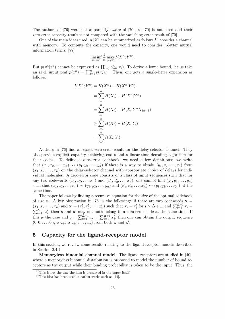
The authors of [76] were not apparently aware of [70], as [70] is not cited and theirzero-error capacity result is not compared with the vanishing error result of [70].

One of the main ideas used in [70] can be summarized as follows:17 consider a channelwith memory. To compute the capacity, one would need to consider n-letter mutualinformation terms: [77]

lim infn→∞

1

nmaxp(xn)

I(Xn;Y n).

But p(yn|xn) cannot be expressed as∏ni=1 p(yi|xi). To derive a lower bound, let us take

an i.i.d. input pmf p(xn) =∏ni=1 p(xi).

18 Then, one gets a single-letter expansion asfollows:

I(Xn;Y n) = H(Xn)−H(Xn|Y n)

=n∑i=1

H(Xi)−H(Xn|Y n)

=n∑i=1

H(Xi)−H(Xi|Y nX1:i−1)

≥n∑i=1

H(Xi)−H(Xi|Yi)

=n∑i=1

I(Xi;Yi).

Authors in [76] find an exact zero-error result for the delay-selector channel. Theyalso provide explicit capacity achieving codes and a linear-time decoding algorithm fortheir codes. To define a zero-error codebook, we need a few definitions: we writethat (x1, x2, . . . , xn) (y1, y2, . . . , yn) if there is a way to obtain (y1, y2, . . . , yn) from(x1, x2, . . . , xn) on the delay-selector channel with appropriate choice of delays for indi-vidual molecules. A zero-error code consists of a class of input sequences such that forany two codewords (x1, x2, . . . , xn) and (x′1, x

′2, . . . , x

′n), one cannot find (y1, y2, . . . , yn)

such that (x1, x2, . . . , xn) (y1, y2, . . . , yn) and (x′1, x′2, . . . , x

′n) (y1, y2, . . . , yn) at the

same time.The paper follows by finding a recursive equation for the size of the optimal codebook

of size n. A key observation in [76] is the following: if there are two codewords x =(x1, x2, . . . , xn) and x′ = (x′1, x

′2, . . . , x

′n) such that xi = x′i for i > ∆ + 1, and

∑∆+1i=1 xi =∑∆+1

i=1 x′i, then x and x′ may not both belong to a zero-error code at the same time. If

this is the case and q =∑∆+1

i=1 xi =∑∆+1

i=1 x′i, then one can obtain the output sequence(0, 0, . . . , 0, q, x∆+2, x∆+3, . . . , xn) from both x and x′.

5 Capacity for the ligand-receptor model

In this section, we review some results relating to the ligand-receptor models describedin Section 2.4.4

Memoryless binomial channel model: The ligand receptors are studied in [40],where a memoryless binomial distribution is proposed to model the number of bound re-ceptors as the output while their binding probability is taken to be the input. Thus, the

17This is not the way the idea is presented in the paper itself.18This idea has been used in earlier works such as [54].

26

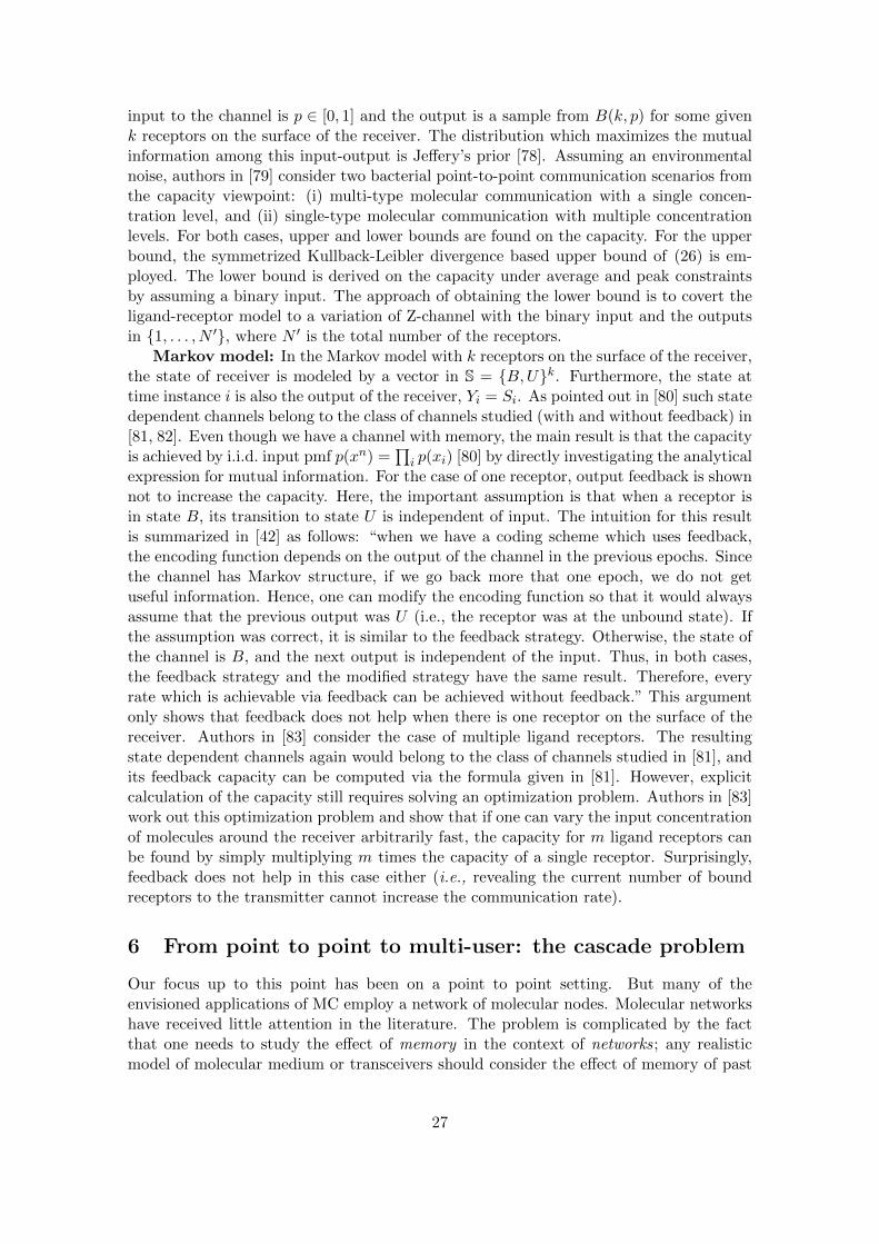
input to the channel is p ∈ [0, 1] and the output is a sample from B(k, p) for some givenk receptors on the surface of the receiver. The distribution which maximizes the mutualinformation among this input-output is Jeffery’s prior [78]. Assuming an environmentalnoise, authors in [79] consider two bacterial point-to-point communication scenarios fromthe capacity viewpoint: (i) multi-type molecular communication with a single concen-tration level, and (ii) single-type molecular communication with multiple concentrationlevels. For both cases, upper and lower bounds are found on the capacity. For the upperbound, the symmetrized Kullback-Leibler divergence based upper bound of (26) is em-ployed. The lower bound is derived on the capacity under average and peak constraintsby assuming a binary input. The approach of obtaining the lower bound is to covert theligand-receptor model to a variation of Z-channel with the binary input and the outputsin {1, . . . , N ′}, where N ′ is the total number of the receptors.

Markov model: In the Markov model with k receptors on the surface of the receiver,the state of receiver is modeled by a vector in S = {B,U}k. Furthermore, the state attime instance i is also the output of the receiver, Yi = Si. As pointed out in [80] such statedependent channels belong to the class of channels studied (with and without feedback) in[81, 82]. Even though we have a channel with memory, the main result is that the capacityis achieved by i.i.d. input pmf p(xn) =

∏i p(xi) [80] by directly investigating the analytical

expression for mutual information. For the case of one receptor, output feedback is shownnot to increase the capacity. Here, the important assumption is that when a receptor isin state B, its transition to state U is independent of input. The intuition for this resultis summarized in [42] as follows: “when we have a coding scheme which uses feedback,the encoding function depends on the output of the channel in the previous epochs. Sincethe channel has Markov structure, if we go back more that one epoch, we do not getuseful information. Hence, one can modify the encoding function so that it would alwaysassume that the previous output was U (i.e., the receptor was at the unbound state). Ifthe assumption was correct, it is similar to the feedback strategy. Otherwise, the state ofthe channel is B, and the next output is independent of the input. Thus, in both cases,the feedback strategy and the modified strategy have the same result. Therefore, everyrate which is achievable via feedback can be achieved without feedback.” This argumentonly shows that feedback does not help when there is one receptor on the surface of thereceiver. Authors in [83] consider the case of multiple ligand receptors. The resultingstate dependent channels again would belong to the class of channels studied in [81], andits feedback capacity can be computed via the formula given in [81]. However, explicitcalculation of the capacity still requires solving an optimization problem. Authors in [83]work out this optimization problem and show that if one can vary the input concentrationof molecules around the receiver arbitrarily fast, the capacity for m ligand receptors canbe found by simply multiplying m times the capacity of a single receptor. Surprisingly,feedback does not help in this case either (i.e., revealing the current number of boundreceptors to the transmitter cannot increase the communication rate).

6 From point to point to multi-user: the cascade problem

Our focus up to this point has been on a point to point setting. But many of theenvisioned applications of MC employ a network of molecular nodes. Molecular networkshave received little attention in the literature. The problem is complicated by the factthat one needs to study the effect of memory in the context of networks; any realisticmodel of molecular medium or transceivers should consider the effect of memory of past

27

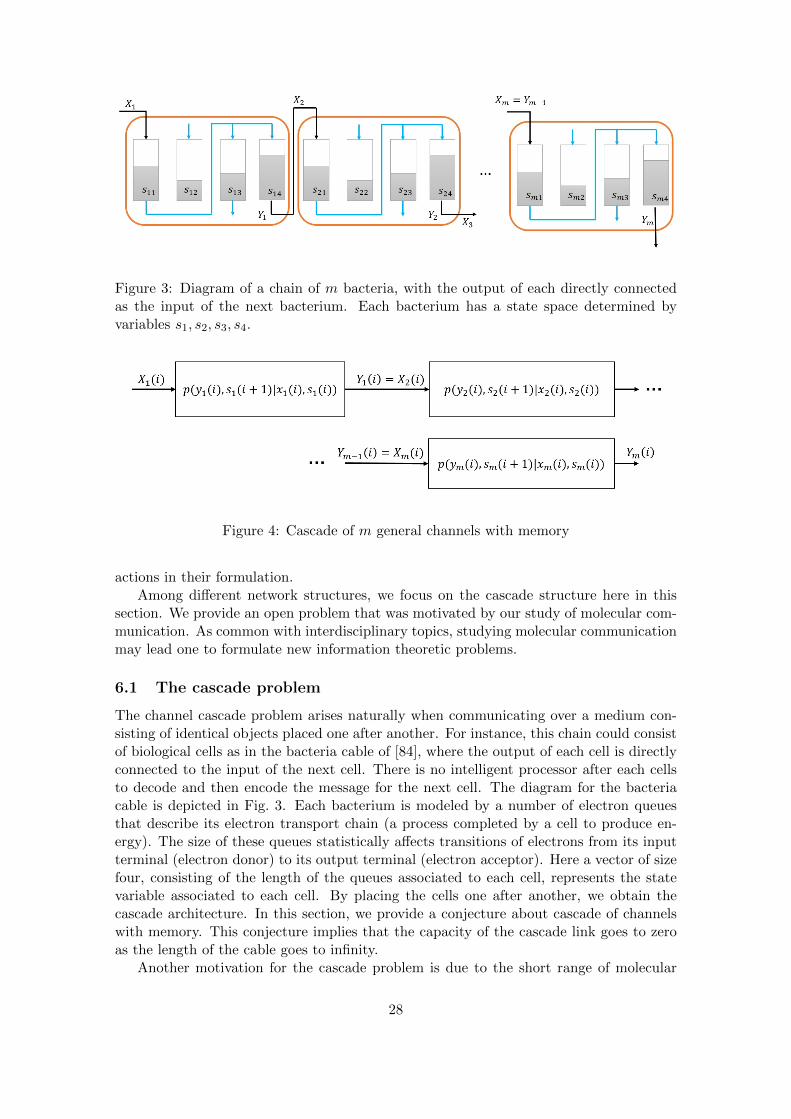
Figure 3: Diagram of a chain of m bacteria, with the output of each directly connectedas the input of the next bacterium. Each bacterium has a state space determined byvariables s1, s2, s3, s4.

Figure 4: Cascade of m general channels with memory

actions in their formulation.Among different network structures, we focus on the cascade structure here in this

section. We provide an open problem that was motivated by our study of molecular com-munication. As common with interdisciplinary topics, studying molecular communicationmay lead one to formulate new information theoretic problems.

6.1 The cascade problem

The channel cascade problem arises naturally when communicating over a medium con-sisting of identical objects placed one after another. For instance, this chain could consistof biological cells as in the bacteria cable of [84], where the output of each cell is directlyconnected to the input of the next cell. There is no intelligent processor after each cellsto decode and then encode the message for the next cell. The diagram for the bacteriacable is depicted in Fig. 3. Each bacterium is modeled by a number of electron queuesthat describe its electron transport chain (a process completed by a cell to produce en-ergy). The size of these queues statistically affects transitions of electrons from its inputterminal (electron donor) to its output terminal (electron acceptor). Here a vector of sizefour, consisting of the length of the queues associated to each cell, represents the statevariable associated to each cell. By placing the cells one after another, we obtain thecascade architecture. In this section, we provide a conjecture about cascade of channelswith memory. This conjecture implies that the capacity of the cascade link goes to zeroas the length of the cable goes to infinity.

Another motivation for the cascade problem is due to the short range of molecular

28

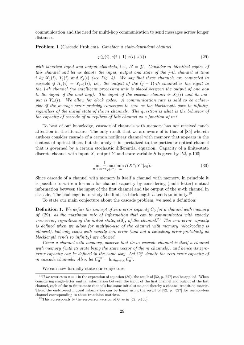
communication and the need for multi-hop communication to send messages across longerdistances.

Problem 1 (Cascade Problem). Consider a state-dependent channel

p(y(i), s(i+ 1)|x(i), s(i)) (29)

with identical input and output alphabets, i.e., X = Y. Consider m identical copies ofthis channel and let us denote the input, output and state of the j-th channel at timei by Xj(i), Yj(i) and Sj(i) (see Fig. 4). We say that these channels are connected incascade if Xj(i) = Yj−1(i), i.e., the output of the (j − 1)-th channel is the input tothe j-th channel (no intelligent processing unit is placed between the output of one hopto the input of the next hop). The input of the cascade channel is X1(i) and its out-put is Ym(i). We allow for block codes. A communication rate is said to be achiev-able if the average error probably converges to zero as the blocklength goes to infinity,regardless of the initial state of the m channels. The question is what is the behavior ofthe capacity of cascade of m replicas of this channel as a function of m?

To best of our knowledge, cascade of channels with memory has not received muchattention in the literature. The only result that we are aware of is that of [85] whereinauthors consider cascade of a certain nonlinear channel with memory that appears in thecontext of optical fibers, but the analysis is specialized to the particular optical channelthat is governed by a certain stochastic differential equation. Capacity of a finite-statediscrete channel with input X, output Y and state variable S is given by [52, p.100]

limn→∞

1

nmaxp(xn)

mins0

I(Xn;Y n|s0). (30)

Since cascade of a channel with memory is itself a channel with memory, in principle itis possible to write a formula for channel capacity by considering (multi-letter) mutualinformation between the input of the first channel and the output of the m-th channel incascade. The challenge is to study the limit as blocklength n tends to infinity.19

To state our main conjecture about the cascade problem, we need a definition:

Definition 1. We define the concept of zero-error capacity C0 for a channel with memoryof (29), as the maximum rate of information that can be communicated with exactlyzero error, regardless of the initial state, s(0), of the channel.20 The zero-error capacityis defined when we allow for multiple-use of the channel with memory (blockcoding isallowed), but only codes with exactly zero error (and not a vanishing error probability asblocklength tends to infinity) are allowed.

Given a channel with memory, observe that its m cascade channel is itself a channelwith memory (with its state being the state vector of the m channels), and hence its zero-error capacity can be defined in the same way. Let Cm0 denote the zero-error capacity ofm cascade channels. Also, let C inf

0 = limm→∞Cm0 .

We can now formally state our conjecture:

19If we restrict to n = 1 in the expression of equation (30), the result of [52, p. 527] can be applied. Whenconsidering single-letter mutual information between the input of the first channel and output of the lastchannel, each of the m finite-state channels has some initial state and thereby a channel transition matrix.Thus, the end-to-end mutual information can be found using the result of [52, p. 527] for memorylesschannel corresponding to these transition matrices.

20This corresponds to the zero-error version of C as in [52, p.100].

29

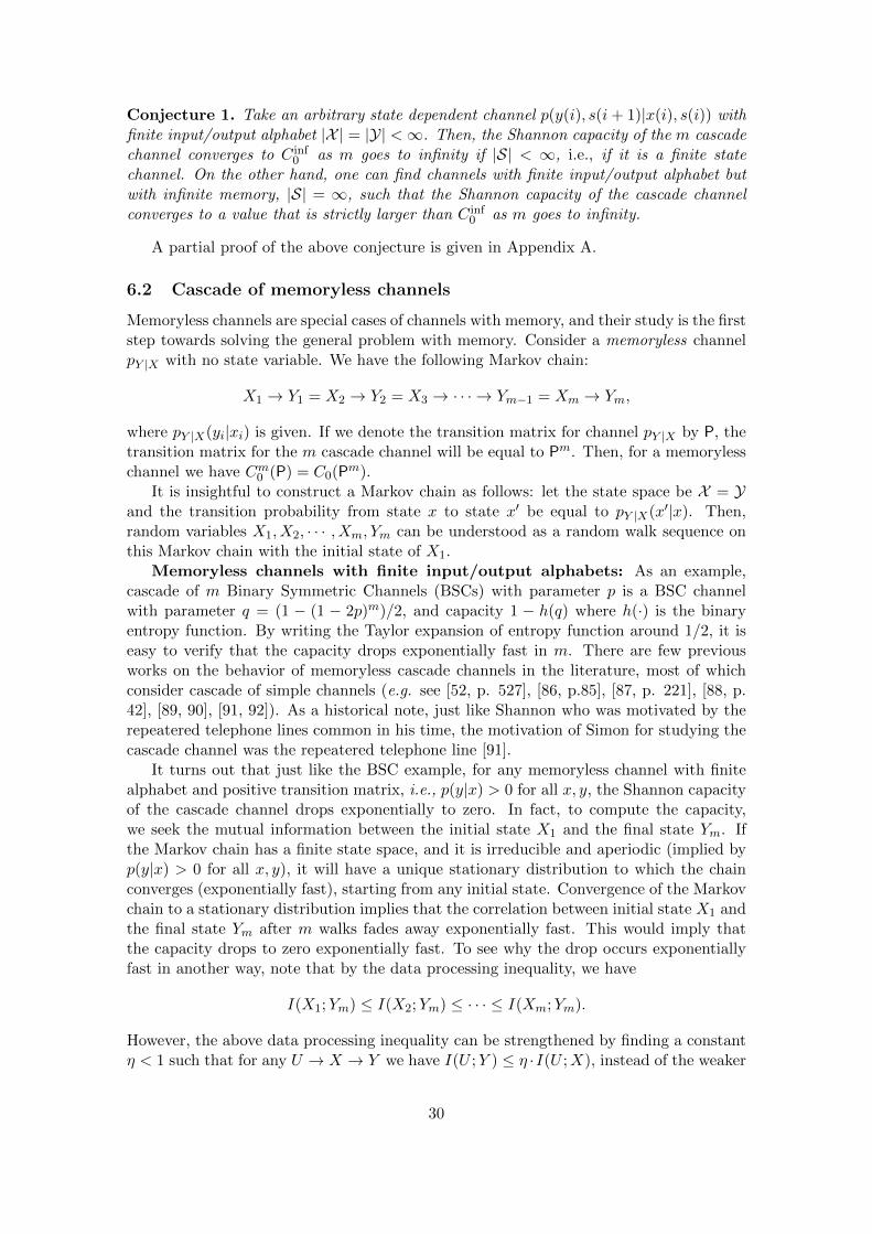
Conjecture 1. Take an arbitrary state dependent channel p(y(i), s(i+ 1)|x(i), s(i)) withfinite input/output alphabet |X | = |Y| <∞. Then, the Shannon capacity of the m cascadechannel converges to C inf

0 as m goes to infinity if |S| < ∞, i.e., if it is a finite statechannel. On the other hand, one can find channels with finite input/output alphabet butwith infinite memory, |S| = ∞, such that the Shannon capacity of the cascade channelconverges to a value that is strictly larger than C inf

0 as m goes to infinity.

A partial proof of the above conjecture is given in Appendix A.

6.2 Cascade of memoryless channels

Memoryless channels are special cases of channels with memory, and their study is the firststep towards solving the general problem with memory. Consider a memoryless channelpY |X with no state variable. We have the following Markov chain:

X1 → Y1 = X2 → Y2 = X3 → · · · → Ym−1 = Xm → Ym,

where pY |X(yi|xi) is given. If we denote the transition matrix for channel pY |X by P, thetransition matrix for the m cascade channel will be equal to Pm. Then, for a memorylesschannel we have Cm0 (P) = C0(Pm).

It is insightful to construct a Markov chain as follows: let the state space be X = Yand the transition probability from state x to state x′ be equal to pY |X(x′|x). Then,random variables X1, X2, · · · , Xm, Ym can be understood as a random walk sequence onthis Markov chain with the initial state of X1.

Memoryless channels with finite input/output alphabets: As an example,cascade of m Binary Symmetric Channels (BSCs) with parameter p is a BSC channelwith parameter q = (1 − (1 − 2p)m)/2, and capacity 1 − h(q) where h(·) is the binaryentropy function. By writing the Taylor expansion of entropy function around 1/2, it iseasy to verify that the capacity drops exponentially fast in m. There are few previousworks on the behavior of memoryless cascade channels in the literature, most of whichconsider cascade of simple channels (e.g. see [52, p. 527], [86, p.85], [87, p. 221], [88, p.42], [89, 90], [91, 92]). As a historical note, just like Shannon who was motivated by therepeatered telephone lines common in his time, the motivation of Simon for studying thecascade channel was the repeatered telephone line [91].

It turns out that just like the BSC example, for any memoryless channel with finitealphabet and positive transition matrix, i.e., p(y|x) > 0 for all x, y, the Shannon capacityof the cascade channel drops exponentially to zero. In fact, to compute the capacity,we seek the mutual information between the initial state X1 and the final state Ym. Ifthe Markov chain has a finite state space, and it is irreducible and aperiodic (implied byp(y|x) > 0 for all x, y), it will have a unique stationary distribution to which the chainconverges (exponentially fast), starting from any initial state. Convergence of the Markovchain to a stationary distribution implies that the correlation between initial state X1 andthe final state Ym after m walks fades away exponentially fast. This would imply thatthe capacity drops to zero exponentially fast. To see why the drop occurs exponentiallyfast in another way, note that by the data processing inequality, we have

I(X1;Ym) ≤ I(X2;Ym) ≤ · · · ≤ I(Xm;Ym).

However, the above data processing inequality can be strengthened by finding a constantη < 1 such that for any U → X → Y we have I(U ;Y ) ≤ η ·I(U ;X), instead of the weaker

30

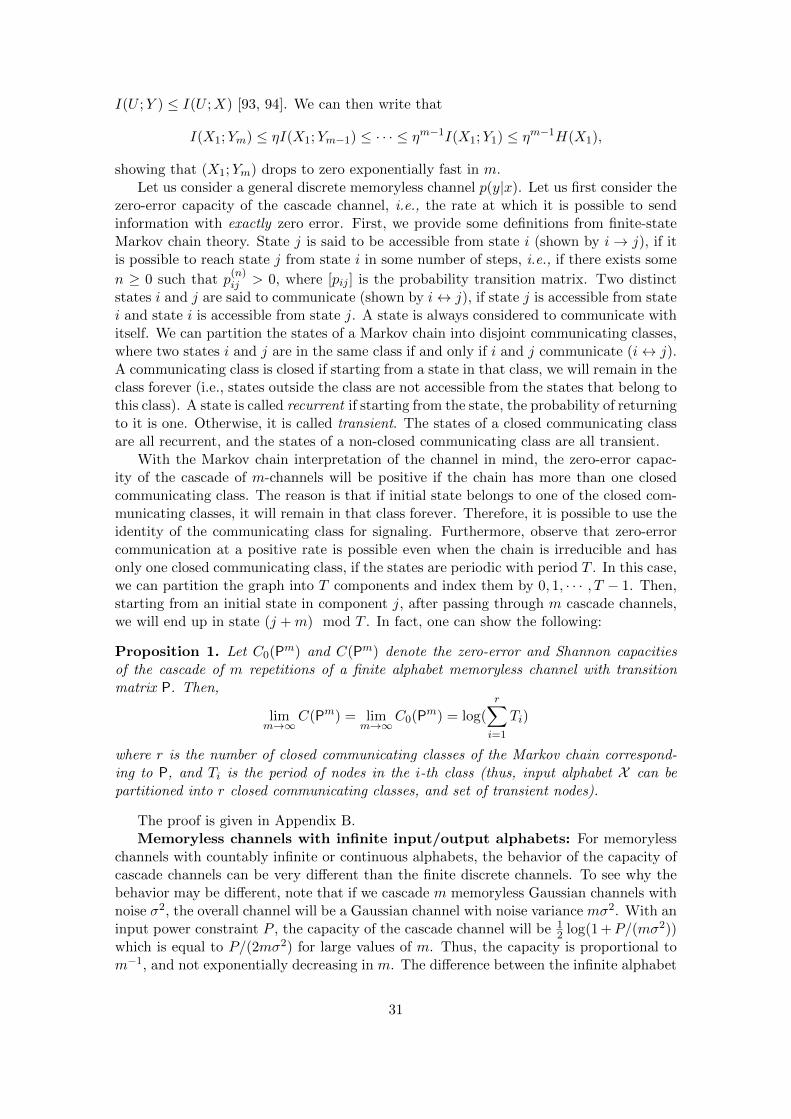
I(U ;Y ) ≤ I(U ;X) [93, 94]. We can then write that

I(X1;Ym) ≤ ηI(X1;Ym−1) ≤ · · · ≤ ηm−1I(X1;Y1) ≤ ηm−1H(X1),

showing that (X1;Ym) drops to zero exponentially fast in m.Let us consider a general discrete memoryless channel p(y|x). Let us first consider the

zero-error capacity of the cascade channel, i.e., the rate at which it is possible to sendinformation with exactly zero error. First, we provide some definitions from finite-stateMarkov chain theory. State j is said to be accessible from state i (shown by i→ j), if itis possible to reach state j from state i in some number of steps, i.e., if there exists some

n ≥ 0 such that p(n)ij > 0, where [pij ] is the probability transition matrix. Two distinct

states i and j are said to communicate (shown by i↔ j), if state j is accessible from statei and state i is accessible from state j. A state is always considered to communicate withitself. We can partition the states of a Markov chain into disjoint communicating classes,where two states i and j are in the same class if and only if i and j communicate (i↔ j).A communicating class is closed if starting from a state in that class, we will remain in theclass forever (i.e., states outside the class are not accessible from the states that belong tothis class). A state is called recurrent if starting from the state, the probability of returningto it is one. Otherwise, it is called transient. The states of a closed communicating classare all recurrent, and the states of a non-closed communicating class are all transient.

With the Markov chain interpretation of the channel in mind, the zero-error capac-ity of the cascade of m-channels will be positive if the chain has more than one closedcommunicating class. The reason is that if initial state belongs to one of the closed com-municating classes, it will remain in that class forever. Therefore, it is possible to use theidentity of the communicating class for signaling. Furthermore, observe that zero-errorcommunication at a positive rate is possible even when the chain is irreducible and hasonly one closed communicating class, if the states are periodic with period T . In this case,we can partition the graph into T components and index them by 0, 1, · · · , T − 1. Then,starting from an initial state in component j, after passing through m cascade channels,we will end up in state (j +m) mod T . In fact, one can show the following:

Proposition 1. Let C0(Pm) and C(Pm) denote the zero-error and Shannon capacitiesof the cascade of m repetitions of a finite alphabet memoryless channel with transitionmatrix P. Then,

limm→∞

C(Pm) = limm→∞

C0(Pm) = log(r∑i=1

Ti)

where r is the number of closed communicating classes of the Markov chain correspond-ing to P, and Ti is the period of nodes in the i-th class (thus, input alphabet X can bepartitioned into r closed communicating classes, and set of transient nodes).

The proof is given in Appendix B.Memoryless channels with infinite input/output alphabets: For memoryless

channels with countably infinite or continuous alphabets, the behavior of the capacity ofcascade channels can be very different than the finite discrete channels. To see why thebehavior may be different, note that if we cascade m memoryless Gaussian channels withnoise σ2, the overall channel will be a Gaussian channel with noise variance mσ2. With aninput power constraint P , the capacity of the cascade channel will be 1

2 log(1 +P/(mσ2))which is equal to P/(2mσ2) for large values of m. Thus, the capacity is proportional tom−1, and not exponentially decreasing in m. The difference between the infinite alphabet

31

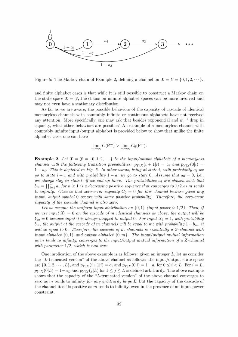
0 1 2 3

1

1− a1

a1

1− a2

a2

1− a3

Figure 5: The Markov chain of Example 2, defining a channel on X = Y = {0, 1, 2, · · · }.

and finite alphabet cases is that while it is still possible to construct a Markov chain onthe state space X = Y, the chains on infinite alphabet spaces can be more involved andmay not even have a stationary distribution.

As far as we are aware, the possible behaviors of the capacity of cascade of identicalmemoryless channels with countably infinite or continuous alphabets have not receivedany attention. More specifically, one may ask that besides exponential and m−1 drop incapacity, what other behaviors are possible? An example of a memoryless channel withcountably infinite input/output alphabet is provided below to show that unlike the finitealphabet case, one can have

limm→∞

C(Pm) > limm→∞

C0(Pm).

Example 2. Let X = Y = {0, 1, 2, · · · } be the input/output alphabets of a memorylesschannel with the following transition probabilities: pY |X(i + 1|i) = ai and pY |X(0|i) =1− ai. This is depicted in Fig. 5. In other words, being at state i, with probability ai wego to state i + 1 and with probability 1 − ai we go to state 0. Assume that a0 = 0, i.e.,we always stay in state 0 if we end up there. The probabilities ai are chosen such thatbm =

∏mi=1 ai for n ≥ 1 is a decreasing positive sequence that converges to 1/2 as m tends

to infinity. Observe that zero-error capacity C0 = 0 for this channel because given anyinput, output symbol 0 occurs with some positive probability. Therefore, the zero-errorcapacity of the cascade channel is also zero.

Let us assume the uniform input distribution on {0, 1} (input power is 1/2). Then, ifwe use input X1 = 0 on the cascade of m identical channels as above, the output will beYm = 0 because input 0 is always mapped to output 0. For input X1 = 1, with probabilitybm, the output at the cascade of m channels will be equal to m; with probability 1− bm, itwill be equal to 0. Therefore, the cascade of m channels is essentially a Z-channel withinput alphabet {0, 1} and output alphabet {0,m}. The input/output mutual informationas m tends to infinity, converges to the input/output mutual information of a Z-channelwith parameter 1/2, which is non-zero.

One implication of the above example is as follows: given an integer L, let us considerthe “L-truncated version” of the above channel as follows: the input/output state spaceare {0, 1, 2, · · · , L}, and pY |X(i+1|i) = ai and pY |X(0|i) = 1−ai for 0 ≤ i < L. For i = L,pY |X(0|L) = 1−aL and pY |X(j|L) for 1 ≤ j ≤ L is defined arbitrarily. The above exampleshows that the capacity of the “L-truncated version” of the above channel converges tozero as m tends to infinity for any arbitrarily large L, but the capacity of the cascade ofthe channel itself is positive as m tends to infinity, even in the presence of an input powerconstraint.

32

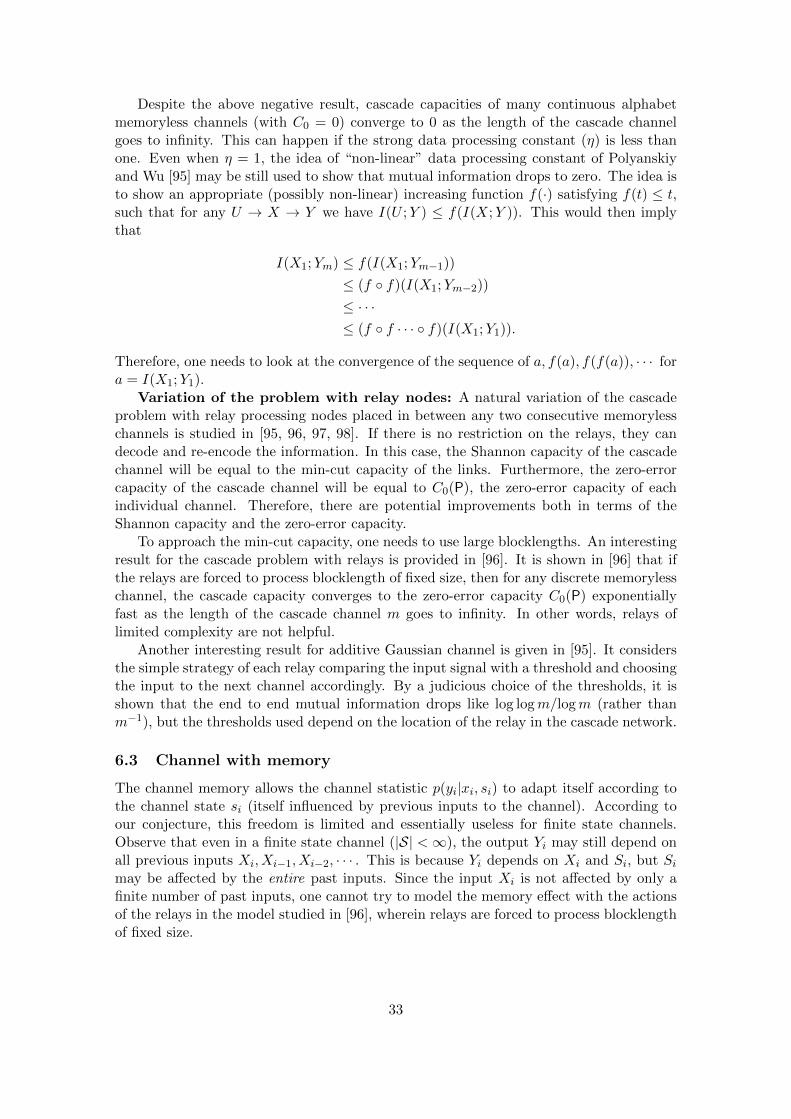
Despite the above negative result, cascade capacities of many continuous alphabetmemoryless channels (with C0 = 0) converge to 0 as the length of the cascade channelgoes to infinity. This can happen if the strong data processing constant (η) is less thanone. Even when η = 1, the idea of “non-linear” data processing constant of Polyanskiyand Wu [95] may be still used to show that mutual information drops to zero. The idea isto show an appropriate (possibly non-linear) increasing function f(·) satisfying f(t) ≤ t,such that for any U → X → Y we have I(U ;Y ) ≤ f(I(X;Y )). This would then implythat

I(X1;Ym) ≤ f(I(X1;Ym−1))

≤ (f ◦ f)(I(X1;Ym−2))

≤ · · ·≤ (f ◦ f · · · ◦ f)(I(X1;Y1)).

Therefore, one needs to look at the convergence of the sequence of a, f(a), f(f(a)), · · · fora = I(X1;Y1).

Variation of the problem with relay nodes: A natural variation of the cascadeproblem with relay processing nodes placed in between any two consecutive memorylesschannels is studied in [95, 96, 97, 98]. If there is no restriction on the relays, they candecode and re-encode the information. In this case, the Shannon capacity of the cascadechannel will be equal to the min-cut capacity of the links. Furthermore, the zero-errorcapacity of the cascade channel will be equal to C0(P), the zero-error capacity of eachindividual channel. Therefore, there are potential improvements both in terms of theShannon capacity and the zero-error capacity.

To approach the min-cut capacity, one needs to use large blocklengths. An interestingresult for the cascade problem with relays is provided in [96]. It is shown in [96] that ifthe relays are forced to process blocklength of fixed size, then for any discrete memorylesschannel, the cascade capacity converges to the zero-error capacity C0(P) exponentiallyfast as the length of the cascade channel m goes to infinity. In other words, relays oflimited complexity are not helpful.

Another interesting result for additive Gaussian channel is given in [95]. It considersthe simple strategy of each relay comparing the input signal with a threshold and choosingthe input to the next channel accordingly. By a judicious choice of the thresholds, it isshown that the end to end mutual information drops like log logm/logm (rather thanm−1), but the thresholds used depend on the location of the relay in the cascade network.

6.3 Channel with memory

The channel memory allows the channel statistic p(yi|xi, si) to adapt itself according tothe channel state si (itself influenced by previous inputs to the channel). According toour conjecture, this freedom is limited and essentially useless for finite state channels.Observe that even in a finite state channel (|S| <∞), the output Yi may still depend onall previous inputs Xi, Xi−1, Xi−2, · · · . This is because Yi depends on Xi and Si, but Simay be affected by the entire past inputs. Since the input Xi is not affected by only afinite number of past inputs, one cannot try to model the memory effect with the actionsof the relays in the model studied in [96], wherein relays are forced to process blocklengthof fixed size.

33

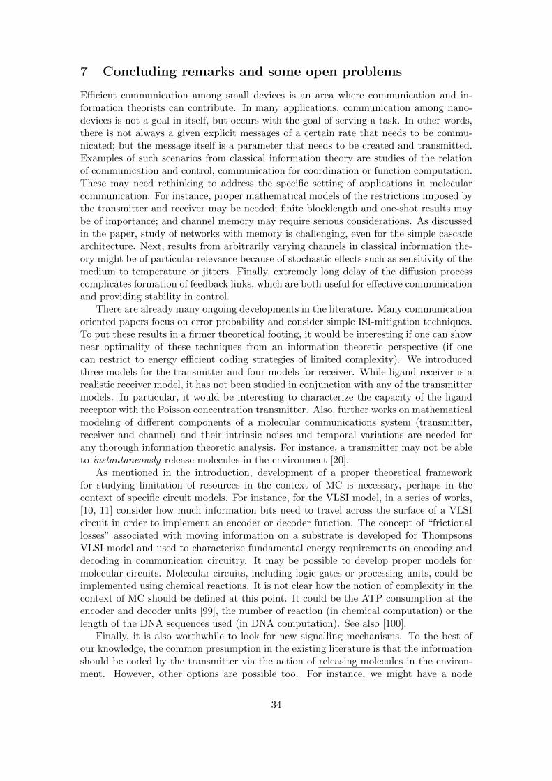
7 Concluding remarks and some open problems

Efficient communication among small devices is an area where communication and in-formation theorists can contribute. In many applications, communication among nano-devices is not a goal in itself, but occurs with the goal of serving a task. In other words,there is not always a given explicit messages of a certain rate that needs to be commu-nicated; but the message itself is a parameter that needs to be created and transmitted.Examples of such scenarios from classical information theory are studies of the relationof communication and control, communication for coordination or function computation.These may need rethinking to address the specific setting of applications in molecularcommunication. For instance, proper mathematical models of the restrictions imposed bythe transmitter and receiver may be needed; finite blocklength and one-shot results maybe of importance; and channel memory may require serious considerations. As discussedin the paper, study of networks with memory is challenging, even for the simple cascadearchitecture. Next, results from arbitrarily varying channels in classical information the-ory might be of particular relevance because of stochastic effects such as sensitivity of themedium to temperature or jitters. Finally, extremely long delay of the diffusion processcomplicates formation of feedback links, which are both useful for effective communicationand providing stability in control.

There are already many ongoing developments in the literature. Many communicationoriented papers focus on error probability and consider simple ISI-mitigation techniques.To put these results in a firmer theoretical footing, it would be interesting if one can shownear optimality of these techniques from an information theoretic perspective (if onecan restrict to energy efficient coding strategies of limited complexity). We introducedthree models for the transmitter and four models for receiver. While ligand receiver is arealistic receiver model, it has not been studied in conjunction with any of the transmittermodels. In particular, it would be interesting to characterize the capacity of the ligandreceptor with the Poisson concentration transmitter. Also, further works on mathematicalmodeling of different components of a molecular communications system (transmitter,receiver and channel) and their intrinsic noises and temporal variations are needed forany thorough information theoretic analysis. For instance, a transmitter may not be ableto instantaneously release molecules in the environment [20].

As mentioned in the introduction, development of a proper theoretical frameworkfor studying limitation of resources in the context of MC is necessary, perhaps in thecontext of specific circuit models. For instance, for the VLSI model, in a series of works,[10, 11] consider how much information bits need to travel across the surface of a VLSIcircuit in order to implement an encoder or decoder function. The concept of “frictionallosses” associated with moving information on a substrate is developed for ThompsonsVLSI-model and used to characterize fundamental energy requirements on encoding anddecoding in communication circuitry. It may be possible to develop proper models formolecular circuits. Molecular circuits, including logic gates or processing units, could beimplemented using chemical reactions. It is not clear how the notion of complexity in thecontext of MC should be defined at this point. It could be the ATP consumption at theencoder and decoder units [99], the number of reaction (in chemical computation) or thelength of the DNA sequences used (in DNA computation). See also [100].

Finally, it is also worthwhile to look for new signalling mechanisms. To the best ofour knowledge, the common presumption in the existing literature is that the informationshould be coded by the transmitter via the action of releasing molecules in the environ-ment. However, other options are possible too. For instance, we might have a node

34

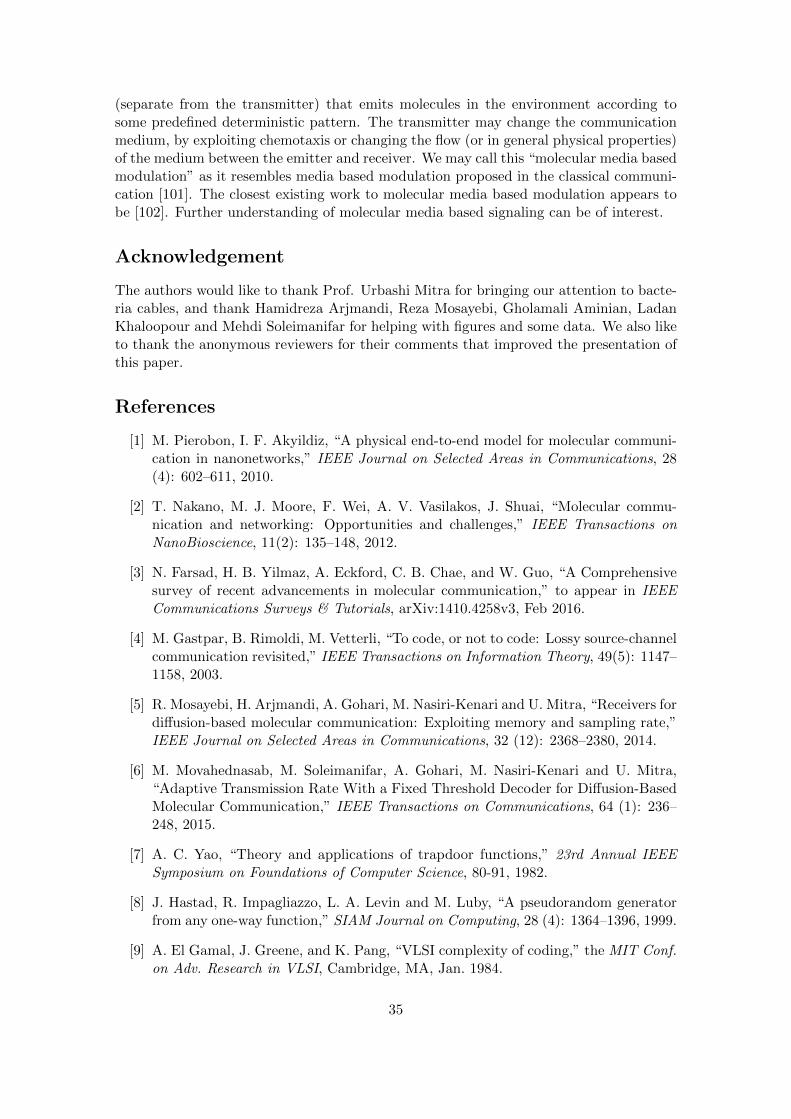
(separate from the transmitter) that emits molecules in the environment according tosome predefined deterministic pattern. The transmitter may change the communicationmedium, by exploiting chemotaxis or changing the flow (or in general physical properties)of the medium between the emitter and receiver. We may call this “molecular media basedmodulation” as it resembles media based modulation proposed in the classical communi-cation [101]. The closest existing work to molecular media based modulation appears tobe [102]. Further understanding of molecular media based signaling can be of interest.

Acknowledgement

The authors would like to thank Prof. Urbashi Mitra for bringing our attention to bacte-ria cables, and thank Hamidreza Arjmandi, Reza Mosayebi, Gholamali Aminian, LadanKhaloopour and Mehdi Soleimanifar for helping with figures and some data. We also liketo thank the anonymous reviewers for their comments that improved the presentation ofthis paper.

References

[1] M. Pierobon, I. F. Akyildiz, “A physical end-to-end model for molecular communi-cation in nanonetworks,” IEEE Journal on Selected Areas in Communications, 28(4): 602–611, 2010.

[2] T. Nakano, M. J. Moore, F. Wei, A. V. Vasilakos, J. Shuai, “Molecular commu-nication and networking: Opportunities and challenges,” IEEE Transactions onNanoBioscience, 11(2): 135–148, 2012.

[3] N. Farsad, H. B. Yilmaz, A. Eckford, C. B. Chae, and W. Guo, “A Comprehensivesurvey of recent advancements in molecular communication,” to appear in IEEECommunications Surveys & Tutorials, arXiv:1410.4258v3, Feb 2016.

[4] M. Gastpar, B. Rimoldi, M. Vetterli, “To code, or not to code: Lossy source-channelcommunication revisited,” IEEE Transactions on Information Theory, 49(5): 1147–1158, 2003.

[5] R. Mosayebi, H. Arjmandi, A. Gohari, M. Nasiri-Kenari and U. Mitra, “Receivers fordiffusion-based molecular communication: Exploiting memory and sampling rate,”IEEE Journal on Selected Areas in Communications, 32 (12): 2368–2380, 2014.

[6] M. Movahednasab, M. Soleimanifar, A. Gohari, M. Nasiri-Kenari and U. Mitra,“Adaptive Transmission Rate With a Fixed Threshold Decoder for Diffusion-BasedMolecular Communication,” IEEE Transactions on Communications, 64 (1): 236–248, 2015.

[7] A. C. Yao, “Theory and applications of trapdoor functions,” 23rd Annual IEEESymposium on Foundations of Computer Science, 80-91, 1982.

[8] J. Hastad, R. Impagliazzo, L. A. Levin and M. Luby, “A pseudorandom generatorfrom any one-way function,” SIAM Journal on Computing, 28 (4): 1364–1396, 1999.

[9] A. El Gamal, J. Greene, and K. Pang, “VLSI complexity of coding,” the MIT Conf.on Adv. Research in VLSI, Cambridge, MA, Jan. 1984.

35

[10] P. Grover, A. Goldsmith and A. Sahai, “Fundamental limits on the power con-sumption of encoding and decoding,” Proc. IEEE Int. Symp. on Inf. Theory (ISIT),2716–2720, 2012.

[11] P. Grover, “Information Friction and Its Implications on Minimum Energy Requiredfor Communication,” IEEE Transactions on Information Theory, 61(2): 895–907,2015.

[12] A. Einolghozati, M. Sardari, and F. Fekri, “Collective sensing-capacity of bacteriapopulations,” Proc. IEEE Int. Symp. on Inf. Theory (ISIT), 2959–2963, 2012.

[13] N. Farsad and A. Goldsmith, “A molecular communication system using acids,bases and hydrogen ions,” 2016 IEEE 17th International Workshop on In SignalProcessing Advances in Wireless Communications (SPAWC), 1–6, 2016.

[14] R. Mosayebi, A. Gohari, M. Mirmohseni, and M. Nasiri-Kenari, “Type based signmodulation for molecular communication,” to appear in Proc. Iran Workshop onCommunication and Information Theory (IWCIT), 2016.

[15] J.G. Andrews, A. Dimakis, L. Dolecek, M. Effros, M. Medard, O. Milenkovic, A.Montanari, S. Vishwanath, E. Yeh, R. Berry, K. Duffy, “A Perspective on FutureResearch Directions in Information Theory,” arXiv preprint arXiv:1507.05941, 2015.

[16] B. W. Andrews and P. A. Iglesias, “An information-theoretic characterization of theoptimal gradient sensing response of cells,” PLoS Computational Biology, 3(8):e153,2007.

[17] M. Pierobon, I. F. Akyildiz, “Diffusion-based noise analysis for molecular commu-nication in nanonetworks,” IEEE Transactions on Signal Processing, 59 (6), 2532-2547, 2011.

[18] C.T. Chou, “A Markovian approach to the optimal demodulation of diffusion-basedmolecular communication networks,” IEEE Transactions on Communications, vol.63, no,10, pp. 3728-3743, Oct. 2015.

[19] P. C. Bressloff, Stochastic processes in cell biology, Heidelberg: Springer, Switzer-land, 2014.

[20] H. Arjmandi, A. Ahmadzadeh, R. Schober, and M. Nasiri-Kenari, “Ion ChannelBased Bio-Synthetic Modulator for Diffusive Molecular Communication,” to appearin IEEE Transactions on NanoBioscience, 2016.

[21] H. Mahdavifar, A. Beirami, “Diffusion channel with Poisson reception process: ca-pacity results and applications,” Proc. IEEE Int. Symp. on Inf. Theory (ISIT),1956–1960, 2015.

[22] C. V. Pao, “Nonlinear parabolic and elliptic equations,” 1992, Plenum Press, NewYork

[23] B. Oksendal, “Stochastic differential equations: an introduction with applications,”Springer-Verlag Berlin Heidelberg, 2003.

[24] W. Feller, “An introduction to probability theory and its applications: volume II,”London-New York-Sydney-Toronto: John Wiley & Sons, 1971.

36

[25] P. E. Protter, “Stochastic Differential Equations. In Stochastic Integration and Dif-ferential Equations,” Springer Berlin Heidelberg, 2005.

[26] B. Cushman-Roisin, “Environmental transport and fate,” Thayer School of Engi-neering Dartmouth College, University Lecture, 2012.

[27] H. Arjmandi, A. Gohari, M. Nasiri-Kenari, and F. Bateni, “Diffusion-based nanonet-working: A new modulation technique and performance analysis,” CommunicationsLetters, IEEE, 17 (4): 645–648, 2013.

[28] M. Pierobon and I. Akyildiz, “Diffusion-based noise analysis for molecular com-munication in nanonetworks,” IEEE Transactions on Signal Processing, 59 (6):2532–2547, 2011.

[29] M. Mahfuz, D. Makrakis, and H. Mouftah, “A comprehensive study of sampling-based optimum signal detection in concentration-encoded molecular communica-tion,” IEEE Transactions on NanoBioscience, 13 (3): 208–222, 2014.

[30] A. Noel, K. Cheung, and R. Schober, “Improving receiver performance of diffusivemolecular communication with enzymes,” IEEE Transactions on NanoBioscience,13 (1): 31–43, 2014.

[31] H. Yilmaz, A. Heren, T. Tugcu, and C.-B. Chae, “Three-dimensional channel char-acteristics for molecular communications with an absorbing receiver,” IEEE Com-munication Letters, 18 (6): 929-932, 2014.

[32] S. Ghavami, R. S. Adve, and F. Lahouti, “Information rates of ask-based molecularcommunication in fluid media,” IEEE Transactions on Molecular, Biological andMulti-Scale Communications, 1 (3): 277291, 2015.

[33] S. M. Ross, Introduction to pobability models (tenth edition), Academic Press, 2010.

[34] N. Farsad, Y. Murin, A. Eckford, A. Goldsmith, “Capacity limits of diffusion-basedmolecular timing channels,” arXiv preprint arXiv:1602.07757, 2016.

[35] K. V. Srinivas, A. W. Eckford, R. S. Adve, “Molecular communication in fluidmedia: The additive inverse gaussian noise channel,” IEEE Transactions on Infor-mation Theory, 58(7), 4678–4692, 2012.

[36] H. B. Yilmaz, A. C. Heren, T. Tugcu, and C.-B. Chae, “Three- dimensional channelcharacteristics for molecular communications with an absorbing receiver,” IEEECommuminications Letters, 18(6): 929-932, 2014.

[37] D. Kilinc, O. B. Akan, “Receiver design for molecular communication,” IEEE Jour-nal on Selected Areas in Communications, 31 (12): 705-714, 2013.

[38] B. Atakan, O. B. Akan, “An information theoretical approach for molecular com-munication,” Bio-Inspired Models of Network, Information and Computing Systems,Bionetics 33–40, 2007.

[39] B. Atakan and O. B. Akan, “Single and multiple-access channel capacity in molec-ular nanonetworks,” Nano-Net, ser. Springer Lect. Notes Inst. Comput. Sci., SocialInf. and Telecommu. Eng., A. Schmid, S. Goel, W. Wang, V. Beiu, and S. Carrara,Eds., 20: 14–23, 2009.

37

[40] A. Einolghozati, M. Sardari, and F. Fekri, “Capacity of diffusion-based molecularcommunication with ligand receptors,” Proc. IEEE Inf. Theory Workshop (ITW),85–89, 2011.

[41] A. W. Eckford, P. J. Thomas, “Capacity of a simple intercellular signal transductionchannel”, Proc. IEEE Int. Symp. on Inf. Theory (ISIT), 1834–1838, 2013.

[42] M. Tahmasbi, F. Fekri, “On the capacity achieving probability measures for molec-ular receivers”, Proc. IEEE Inf. Theory Workshop (ITW), 109–113, 2015.

[43] A. Ahmadzadeh, H. Arjmandi, A. Burkovski, R. Schober, “Comprehensive Reac-tive Receiver Modeling for Diffusive Molecular Communication Systems: ReversibleBinding, Molecule Degradation, and Finite Number of Receptors,” IEEE Transac-tions on NanoBioscience, 2016.

[44] M. Pierobon and I. Akyildiz, “Noise analysis in ligand-binding reception for molec-ular communication in nanonetworks,” IEEE Transactions on Signal Processing,59(9): 4168–4182, 2011.

[45] C. T. Chou, “Impact of receiver reaction mechanisms on the performance of molecu-lar communication networks,” IEEE Transactions on Nanotechnology, 14 (2): 304–317, 2015.

[46] A. C. Heren, H. B. Yilmaz, C. B. Chae, T. Tugcu, “Effect of Degradation in Molecu-lar Communication: Impairment or Enhancement?,” IEEE Transactions on Molec-ular, Biological and Multi-Scale Communications, 1(2): 217–229, 2015.

[47] A. W. Eckford, “Nanoscale communication with brownian motion,” in Proc. Conf.on Inf. Sci. and Syst. (CISS), 160-165, 2007.

[48] C. Rose, C., I. S. Mian, “Signaling with identical tokens: Lower bounds with energyconstraints,” Proc. IEEE Int. Symp. on Inf. Theory (ISIT), 1839–1843, 2013.

[49] C. Rose and I. Mian, “A fundamental framework for molecular communicationchannels: Timing & payload,” Proc. IEEE Int. Conf. on Commun. (ICC), 1043–1048, 2015.

[50] D. Arifler, “Capacity analysis of a diffusion-based short-range molecular nano-communication channel,” Computer Networks, 55(6), 1426-1434, 2011.

[51] G. Aminian, H. Arjmandi, A. Gohari, M. Nasiri-Kenari, and U. Mitra, “Capacity ofdiffusion based molecular communication networks in the LTI-Poisson model,”IEEETransactions on Molecular, Biological and Multi-Scale Communications, 1(2): 188–201, 2015.

[52] R. G. Gallager, Information Theory and Reliable Communication. New York Wiley,1968.

[53] W. Hirt and J. L. Massey, “Capacity of the discrete-time Gaussian channel withintersymbol interference,” IEEE Transactions on Information Theory, 34(3):38–38,1988.

[54] S. Shamai, L. Ozarow, and A. Wyner, “Information rates for a discretetime gaussianchannel with intersymbol interference and stationary inputs, IEEE Transactions onInformation Theory, 37(6): 15271539, 1991.

38

[55] B. Atakan and O. B. Akan, “On channel capacity and error compensation in molecu-lar communication,” Trans. Comput. Syst. Biol. X, ser. Springer Lect. Notes Com-put. Sci., C. Priami, F. Dressler, O. B. Akan, and A. Ngom, Eds., 5410: 59–80,2008.

[56] Q. Liu, and K. Yang, “Channel capacity analysis of a diffusion-based molecular com-munication system with ligand receptors,” International Journal of CommunicationSystems, 28(8):1508–1520, 2014.

[57] A. Einolghozati, M. Sardari, and F. Fekri, “Design and analysis of wireless commu-nication systems using diffusion-based molecular communication among bacteria,”IEEE Transactions on Wireless Communications, 12(12): 6096–6105, 2013.

[58] A. Einolghozati, M. Sardari, and F. Fekri, “Relaying in diffusion-based molecularcommunication,” Proc. IEEE Int. Symp. on Inf. Theory (ISIT), 1844–1848, 2013.

[59] A. Einolghozati, M. Sardari, and F. Fekri, “Decode and forward relaying in diffusion-based molecular communication between two populations of biological agents,”Proc. IEEE Int. Conf. on Commun. (ICC), 3975–3980, 2014.

[60] M. S. Kuran, H. B. Yilmaz, T. Tugcu, and B. Ozerman, “Energy model for com-munication via diffusion in nanonetworks,” Elsevier Nano Commun. Netw., 1(2):86–95, 2010.

[61] A. Lapidoth, J. H. Shapiro, V. Venkatesan, and L. Wang, “The discrete-time poissonchannel at low input powers,” IEEE Transactions on Information Theory, 57(6):3260–3272, 2011.

[62] A. Lapidoth and S. M. Moser, “On the capacity of the discrete-time poisson chan-nel,” IEEE Transactions on Information Theory, 55(1):303–322, 2009.

[63] Y. Chahibi and I. F. Akyildiz, “Molecular Communication Noise and CapacityAnalysis for Particulate Drug Delivery Systems”, IEEE Transactions on Commu-nications, 62 (11), 3891–3903, 2014.

[64] S. Verdu, “Multiple-access channels with memory with and without frame synchro-nism,” IEEE Transactions on Information Theory, 35(3): 605–619, 1989.

[65] D. P. Palomar, S. Verdu, “Lautum information,” IEEE Transactions on InformationTheory, 54(3): 964–975, 2008.

[66] M. Mitzenmacher and E. Upfal, Probability and computing: randomized algorithmsand probabilistic analysis, Cambridge University Press, 2005.

[67] A. Einolghozati, M. Sardari, A. Beirami, and F. Fekri, “Capacity of discrete molec-ular diffusion channels,” Proc. IEEE Int. Symp. on Inf. Theory (ISIT), 723–727,2011.

[68] V. Anantharam and S. Verdu, “Bits through queues, IEEE Transactions on Infor-mation Theory, 42(1): 4-18, 1996.

[69] C. Rose, C., I. S. Mian, “Signaling with identical tokens: Upper bounds with energyconstraints,” Proc. IEEE Int. Symp. on Inf. Theory (ISIT), 1817–1821, 2014.

39

[70] L. Cui, A. W. Eckford, “The delay selector channel: Definition and capacitybounds,” IEEE Canadian Workshop on Information Theory (CWIT), 15–18, 2011.

[71] F. Topsoe, “An information theoretical identity and a problem involving capacity,”Studia Scientiarum Math. Hungarica, 2:291292, 1967.

[72] M. N. Khormuji, “On the capacity of molecular communication over the AIGNchannel,” Proc. Conf. on Inf. Sci. and Syst. (CISS), 1–4, 2011.

[73] H. Li, S. Moser, and D. Guo, “Capacity of the memoryless additive inverse gaussiannoise channel,” IEEE Journal on Selected Areas in Communications, 32(12): 2315–2329, 2014.

[74] W. Schwarz, “On the convolution of inverse Gaussian and exponential random vari-ables,” Communications in Statistics Theory and Methods, 31(12): 2113–2121,2002.

[75] A.W. Eckford, C. B. Chae “Scaling laws for molecular communication”, Proc. IEEEInt. Symp. on Inf. Theory (ISIT), 1281–1285, 2014.

[76] M. Kovacevic, P. Popovski, “Zero-error capacity of a class of timing channels,”IEEE Transactions on Information Theory, 60(11), 6796–6800, 2014.

[77] S. Verdu, T. S. Han, “A general formula for channel capacity,” IEEE Transactionson Information Theory, 40 (4), 1147-1157, 1994.

[78] Q. Xie and A. R. Barron, “Minimax redundancy for the class of memorylesssources,” IEEE Transactions on Information Theory, 43(2): 646–657, 1997.

[79] G. Aminian, M. Farahnak-Ghazani, M. Mirmohseni, M. Nasiri-Kenari, and F. Fekri,“On the Capacity of Point-to-Point and Multiple-Access Molecular Communicationswith Ligand-Receptors,” to appear in IEEE Transactions on Molecular, Biologicaland Multi-Scale Communications, 2016.

[80] P. J. Thomas, A. W. Eckford, A. W. “Shannon Capacity of Signal Transduction forMultiple Independent Receptors,” arXiv preprint arXiv:1604.03508, 2016.

[81] J. Chen and T. Berger, The capacity of finite-state Markov channels with feedback,IEEE Transactions on Information Theory, 51(3): 780–798, 2005.

[82] H. H. Permuter, H. Asnani, and T. Weissman, “Capacity of a POST channel withand without feedback, IEEE Transactions on Information Theory, 60(10): 6041–6057, 2014.

[83] P. J. Thomas, A. Eckford “Shannon Capacity of Signal Transduction for MultipleIndependent Receptors,” IEEE International Symposium on Information Theory(ISIT), 1804–1808, 2016.

[84] N. Michelusi, S. Pirbadian, M.Y. El-Naggar, U. Mitra, “A Stochastic Model forElectron Transfervin Bacterial Cables”, IEEE Journal on Selected Areas in Com-munication, 32(12): 2402–2416, 2014.

[85] G. Kramer, M. I. Yousefi and F. R. Kschischang, “Upper bound on the capacity ofa cascade of nonlinear and noisy channels,” IEEE Information Theory Workshop(ITW), 1-4, 2015.

40

[86] R. B. Ash, Information Theory, New York Wiley, 1965

[87] T. M. Cover and J. A. Thomas, Elements of Information Theory, New York Wdey,1991.

[88] R. J. McEliece, The Theory of Information and Coding, Reading, MA: Addison-Wesley, 1977

[89] Aaron B. Kiely and John T. Coffey, “On the capacity of a cascade of channels”,IEEE Transactions on Information Theory, 39 (4):1310–1321, 1993.

[90] E. Majani, “A model for the study of very noisy channels, and applications,” Ph.D.dissertation, California Inst. of Technol., Pasadena, CA, 1988.

[91] M.K. Simon, “On the capacity of a cascade of identical discrete memoryless nonsin-gular channels,” IEEE Transactions on Information Theory, 16(1): 100-102, 1970.

[92] R.A. Siveman, “On binary channels and their cascades,” IRE Transactions on In-formation Theory, 1(3): 19-27, 1955.

[93] R. Ahlswede and P. Gacs, “Spreading of sets in product spaces and hypercontractionof the Markov operator,” Annals of Probability, 925-939, 1976.

[94] V. Anantharam, A. Gohari, S. Kamath, and C. Nair. “On maximal correlation,hypercontractivity, and the data processing inequality studied by Erkip and Cover,”arXiv preprint arXiv:1304.6133, 2013.

[95] Y. Polyanskiy and Y. Wu, “Dissipation of information in channels with input con-straints,” IEEE Transactions on Information Theory, 62 (1), 35–55, 2016.

[96] U. Niesen, C. Fragouli, D. Tuninetti, “On the capacity of line networks,” IEEETransactions on Information Theory, 53 (11), 4039–4058, 2007.

[97] R. Subramanian, B. N. Vellambi, and I. Land. “An improved bound on informationloss due to finite block length in a Gaussian line network,” Proc. IEEE Int. Symp.on Inf. Theory (ISIT), 1864–1868, 2013.

[98] R. Subramanian, “The relation between block length and reliability for a cascadeof AWGN links,” Proc. 2012 Int. Zurich Seminar on Communications (IZS), 71-74,2012.

[99] Y. Lu, M. D. Higgins, M. S. Leeson, “Comparison of channel coding schemes forMolecular Communications Systems,” IEEE Transactions on Communications, 63(11): 3991 – 4001, 2015.

[100] N. Farsad, H. B. Yilmaz, C. B. Chae, A. Goldsmith, “Energy Model for Vesicle-Based Active Transport Molecular Communication,” arXiv:1510.05075 (2015).

[101] A. K. Khandani, “Media-based modulation: A new approach to wireless transmis-sion,” Proc. IEEE Int. Symp. on Inf. Theory (ISIT), 3050–3054, 2013.

[102] T. Nakano, T. Suda, M. J. Moore, “Molecular Communication through BiologicalPattern Formation,” IEEE Global Communications Conference (GLOBECOM), 1–7, 2015.

[103] C. A. Charalambides, Enumerative combinatorics, CRC Press, 2002.

41

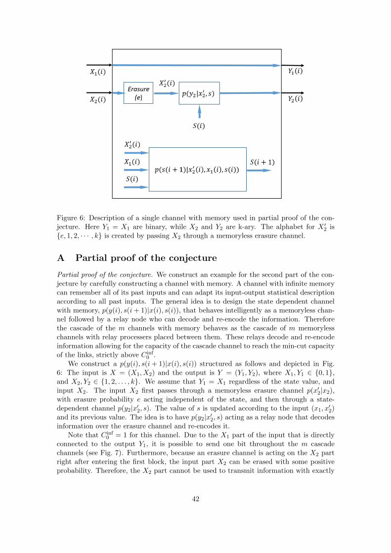
Figure 6: Description of a single channel with memory used in partial proof of the con-jecture. Here Y1 = X1 are binary, while X2 and Y2 are k-ary. The alphabet for X ′2 is{e, 1, 2, · · · , k} is created by passing X2 through a memoryless erasure channel.

A Partial proof of the conjecture

Partial proof of the conjecture. We construct an example for the second part of the con-jecture by carefully constructing a channel with memory. A channel with infinite memorycan remember all of its past inputs and can adapt its input-output statistical descriptionaccording to all past inputs. The general idea is to design the state dependent channelwith memory, p(y(i), s(i+ 1)|x(i), s(i)), that behaves intelligently as a memoryless chan-nel followed by a relay node who can decode and re-encode the information. Thereforethe cascade of the m channels with memory behaves as the cascade of m memorylesschannels with relay processers placed between them. These relays decode and re-encodeinformation allowing for the capacity of the cascade channel to reach the min-cut capacityof the links, strictly above C inf

0 .We construct a p(y(i), s(i+ 1)|x(i), s(i)) structured as follows and depicted in Fig.

6: The input is X = (X1, X2) and the output is Y = (Y1, Y2), where X1, Y1 ∈ {0, 1},and X2, Y2 ∈ {1, 2, . . . , k}. We assume that Y1 = X1 regardless of the state value, andinput X2. The input X2 first passes through a memoryless erasure channel p(x′2|x2),with erasure probability e acting independent of the state, and then through a state-dependent channel p(y2|x′2, s). The value of s is updated according to the input (x1, x

′2)

and its previous value. The idea is to have p(y2|x′2, s) acting as a relay node that decodesinformation over the erasure channel and re-encodes it.

Note that C inf0 = 1 for this channel. Due to the X1 part of the input that is directly

connected to the output Y1, it is possible to send one bit throughout the m cascadechannels (see Fig. 7). Furthermore, because an erasure channel is acting on the X2 partright after entering the first block, the input part X2 can be erased with some positiveprobability. Therefore, the X2 part cannot be used to transmit information with exactly

42

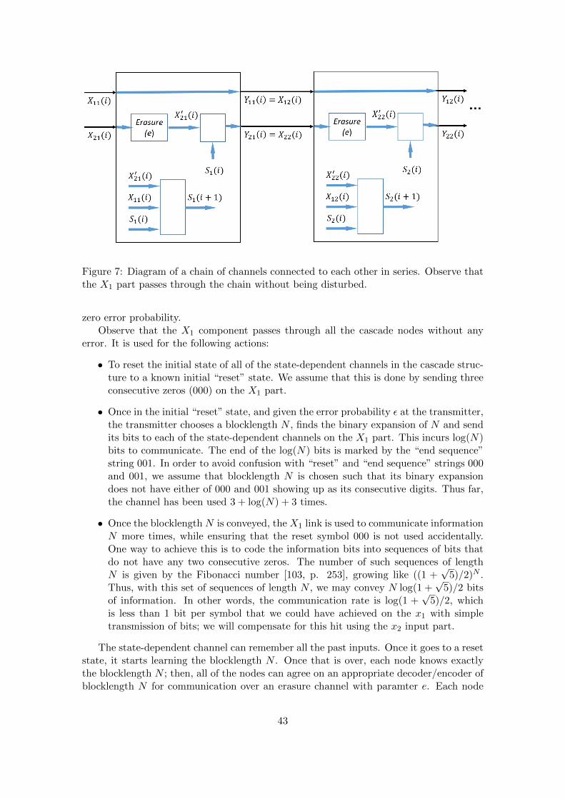
Figure 7: Diagram of a chain of channels connected to each other in series. Observe thatthe X1 part passes through the chain without being disturbed.

zero error probability.Observe that the X1 component passes through all the cascade nodes without any

error. It is used for the following actions:

• To reset the initial state of all of the state-dependent channels in the cascade struc-ture to a known initial “reset” state. We assume that this is done by sending threeconsecutive zeros (000) on the X1 part.

• Once in the initial “reset” state, and given the error probability ε at the transmitter,the transmitter chooses a blocklength N , finds the binary expansion of N and sendits bits to each of the state-dependent channels on the X1 part. This incurs log(N)bits to communicate. The end of the log(N) bits is marked by the “end sequence”string 001. In order to avoid confusion with “reset” and “end sequence” strings 000and 001, we assume that blocklength N is chosen such that its binary expansiondoes not have either of 000 and 001 showing up as its consecutive digits. Thus far,the channel has been used 3 + log(N) + 3 times.

• Once the blocklength N is conveyed, the X1 link is used to communicate informationN more times, while ensuring that the reset symbol 000 is not used accidentally.One way to achieve this is to code the information bits into sequences of bits thatdo not have any two consecutive zeros. The number of such sequences of lengthN is given by the Fibonacci number [103, p. 253], growing like ((1 +

√5)/2)N .

Thus, with this set of sequences of length N , we may convey N log(1 +√

5)/2 bitsof information. In other words, the communication rate is log(1 +

√5)/2, which

is less than 1 bit per symbol that we could have achieved on the x1 with simpletransmission of bits; we will compensate for this hit using the x2 input part.

The state-dependent channel can remember all the past inputs. Once it goes to a resetstate, it starts learning the blocklength N . Once that is over, each node knows exactlythe blocklength N ; then, all of the nodes can agree on an appropriate decoder/encoder ofblocklength N for communication over an erasure channel with paramter e. Each node

43

begins looking at the X2 part of their input for the next N symbols. To produce Y2, eachnode simulates the appropriate decoder/encoder for the blocklength N on the erasurechannel. Because the capacity of the erasure channel is (1−e) log(k), this would allow forreliable transmission of N((1− e) log(k)− ε) bits of information with error probability εon each hop. The total error probability will be at most mε where m is the length of thecascade. This can be made arbitrarily close to zero for a given m by sending blocklengthN to infinity and ε to zero.

The total number of bits that are communicated is N log(1+√

5)/2+N((1−e) log(k)−ε), and the channel is used 3 + log(N) + 3 + N times. This gives us the rate log(1 +√

5)/2) + (1− e) log(k) by letting N converge to infinity and ε converge to zero. Observethat log(1+

√5)/2+(1−e) log(k) can be made arbitrarily larger than C inf

0 = 1 by makingk large.

B Proof of Proposition 1

Observe that C0(Pm) ≥ log(∑r

i=1 Ti) for any m. To see this, note that by choosing anarbitrary vertex from communicating class i and partition j ∈ {0, 1, 2, · · · , Ti − 1}, wecan perfectly predict that after going through m channels, the final state is in commu-nicating class i and partition k = (m + j) mod Ti. Therefore, we can use our choice ofcommunicating class and one of its partitions for signaling with zero error probability.Thus,

limm→∞

C0(Pm) ≥ log(r∑i=1

Ti).

Because for each m, C(Pm) ≥ C0(Pm), it only remains to show that

limm→∞

C(Pm) ≤ log(

r∑i=1

Ti).

Let us assume that X =⋃ri=0 Vi where V0 is the set of transient nodes, and Vi for

i ∈ [1 : r] is the i-th closed communicating class. Furthermore, for i ∈ [1 : r], the inducedgraph on Vi is Ti-partite and we can correspondingly partition Vi into Ti sets Vij , having

Vi =⋃Tij=1 Vij .

It suffices to show that for any arbitrary p(x1) on X1,

limm→∞

I(X1;Ym) ≤ log(r∑i=1

Ti).

We prove this statement in three steps.Case (i): the support of p(x1) is a subset of Vij for some i ∈ [1 : r], j ∈ [1 : Ti]. In

other words, X1 is in the j-th partition of the i-th communicating class. Observe thatI(X1;Ym) is a decreasing sequence in m, by the data processing inequality. Therefore, itsuffices to study the limit for the subsequence defined by m = `Ti for ` = 1, 2, · · · . But ifX1 is in the j-th partition of the i-th communicating class, after `Ti steps, it will return tothe same partition of the same communicating class. Therefore, we can define a reducedMarkov chain on nodes in the j-th partition of the i-th communicating class that specifiesthe transition probabilities after Ti steps. This Markov chain is irreducible and aperiodic.Therefore, it has a unique stationary pmf π to which the chain converges regardless ofinitial state X1. Thus, H(Y`Ti) and H(Y`Ti |X1 = x1) both tend to the entropy of π as `

44

converges to infinity, for any arbitrary x1 in Vij . This implies that limm→∞ I(X1;Ym) iszero in this case.

Case (ii): p(x1) = 0 for all x1 ∈ V0. Let random variable Q ∈ {(i, j) : i ∈ [1 : r], j ∈[1 : Ti]} denote the index of the communicating class and the corresponding partitionthat X1 belongs to. From our earlier discussion Q is a deterministic function of both X1

and Ym. Thus,

I(X1;Ym) = H(Q) + I(X1;Ym|Q)

≤ log |Q|+ I(X1;Ym|Q)

= log(

r∑i=1

Ti) +∑q

I(X1;Ym|Q = q)p(Q = q).

By case (i) and the fact that p(x1|q) is concentrated on one of the partitions of a commu-nicating classes, we have that for any q:

limm→∞

I(X1;Ym|Q = q) = 0.

Therefore,

limm→∞

I(X1;Ym) ≤ log(

r∑i=1

Ti).

Case (iii): arbitrary p(x1). Since V0 is the class of transient states, we have

limm→∞

P[Xm ∈ V0] = 0.

Thus, for any δ > 0, one can find some m0 such that P[Xm0 ∈ V0] < δ. Let U be anindicator function that Xm0 ∈ V0. Then,

I(X1;Ym) ≤ I(Xm0 ;Ym)

= I(UXm0 ;Ym)

≤ H(U) + I(Xm0 ;Ym|U)

≤ h(δ) + δI(Xm0 ;Ym|U = 0) + (1− δ)I(Xm0 ;Ym|U = 1)

≤ h(δ) + δ log |X |+ (1− δ)I(Xm0 ;Ym|U = 1)

Now, conditioned on U = 1, the pmf of p(xm0 |u = 1) falls in the class of pmfs studied incase (ii). Therefore, limm→∞ I(Xm0 ;Ym|U = 1) ≤ log(

∑ri=1 Ti). Hence,

limm→∞

I(X1;Ym) ≤ h(δ) + δ log |X |+ (1− δ) log(r∑i=1

Ti).

We obtain the desired result by letting δ tend to zero.

45