InformedInformedSearchSearch

Yun Peng Modified by M. Perkowski.

Informed Methods Add Domain-Specific Information

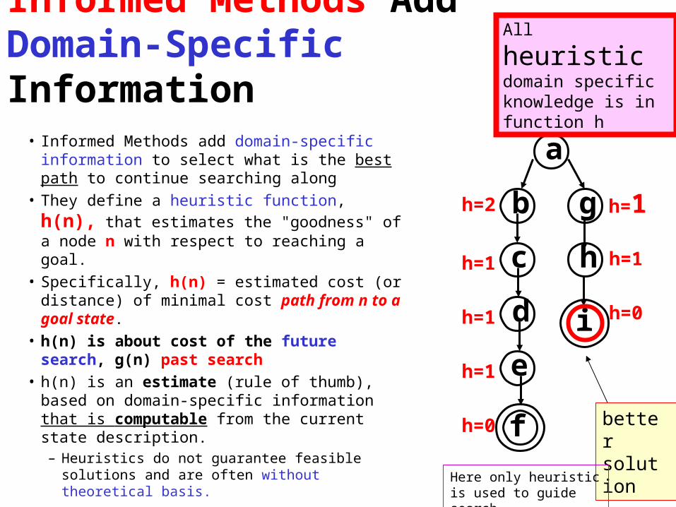
• Informed Methods add domain-specific information to select what is the best path to continue searching along

• They define a heuristic function, h(n), that estimates the "goodness" of a node n with respect to reaching a goal.

• Specifically, h(n) = estimated cost (or distance) of minimal cost path from n to a goal state.

• h(n) is about cost of the future search, g(n) past search

• h(n) is an estimate (rule of thumb), based on domain-specific information that is computable from the current state description.

– Heuristics do not guarantee feasible solutions and are often without theoretical basis.

a

gb

c

d

e

f

h

i

h=2

h=1

h=1

h=1

h=0

h=1

h=1

h=0

better solution

All heuristic domain specific knowledge is in function h

Here only heuristic is used to guide search

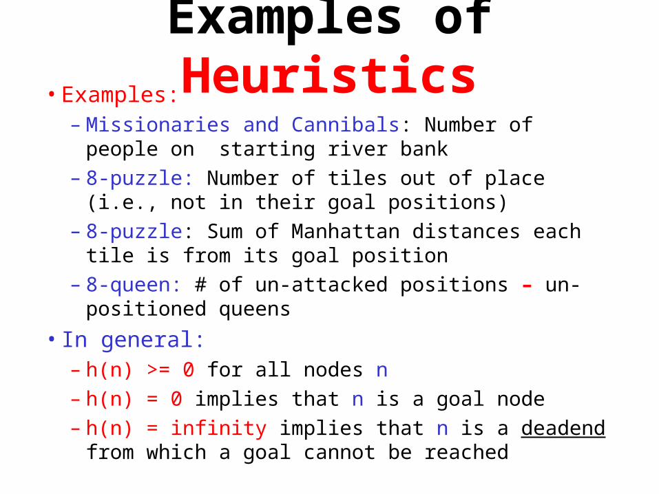
Examples of Heuristics• Examples:

– Missionaries and Cannibals: Number of people on starting river bank

– 8-puzzle: Number of tiles out of place (i.e., not in their goal positions)

– 8-puzzle: Sum of Manhattan distances each tile is from its goal position

– 8-queen: # of un-attacked positions – un-positioned queens

• In general:– h(n) >= 0 for all nodes n

– h(n) = 0 implies that n is a goal node

– h(n) = infinity implies that n is a deadend from which a goal cannot be reached

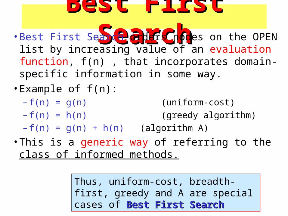
Best First SearchBest First Search• Best First Search orders nodes on the OPEN list by

increasing value of an evaluation function, f(n) , that incorporates domain-specific information in some way.

• Example of f(n): – f(n) = g(n) (uniform-cost)

– f(n) = h(n) (greedy algorithm)

– f(n) = g(n) + h(n) (algorithm A)

• This is a generic way of referring to the class of informed methods.

Thus, uniform-cost, breadth-first, greedy and A are special cases of Best First SearchBest First Search

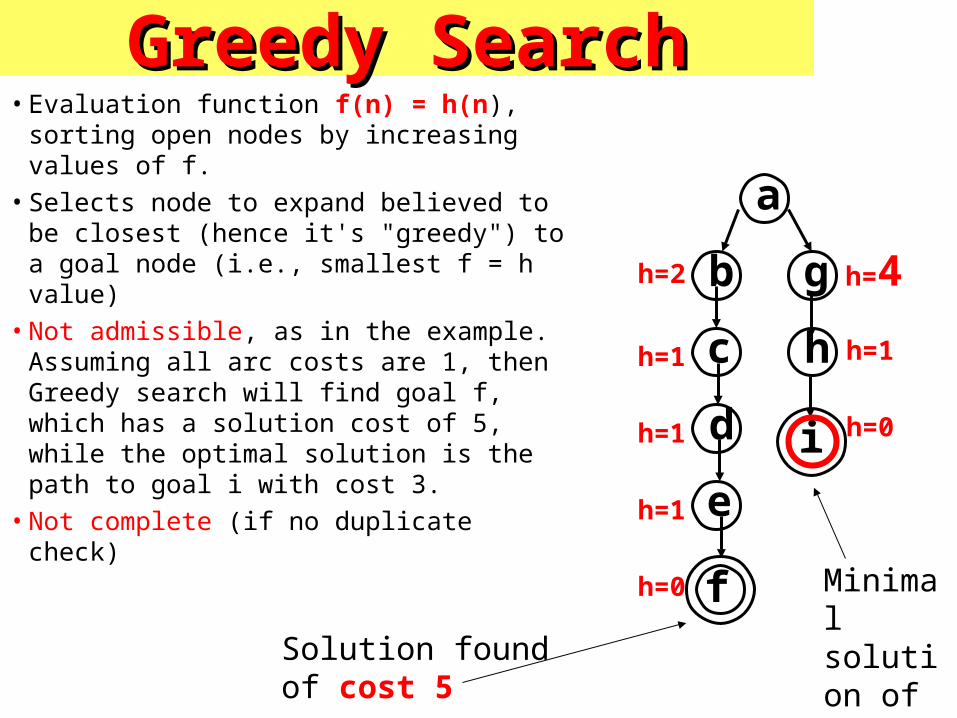
Greedy SearchGreedy Search• Evaluation function f(n) = h(n), sorting

open nodes by increasing values of f.

• Selects node to expand believed to be closest (hence it's "greedy") to a goal node (i.e., smallest f = h value)

• Not admissible, as in the example. Assuming all arc costs are 1, then Greedy search will find goal f, which has a solution cost of 5, while the optimal solution is the path to goal i with cost 3.

• Not complete (if no duplicate check)

a

gb

c

d

e

f

h

i

h=2

h=1

h=1

h=1

h=0

h=4

h=1

h=0

Solution found of cost 5

Minimal solution of cost 3

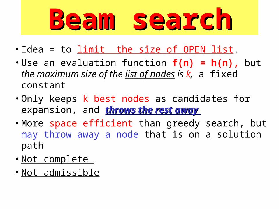
Beam searchBeam search• Idea = to limit the size of OPEN list.

• Use an evaluation function f(n) = h(n), but the maximum size of the list of nodes is k, a fixed constant

• Only keeps k best nodes as candidates for expansion, and throws throws the rest away the rest away

• More space efficient than greedy search, but may throw away a node that is on a solution path

• Not complete

• Not admissible

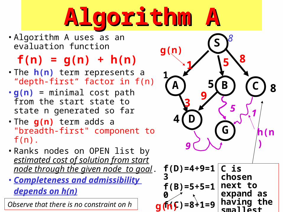
Algorithm AAlgorithm A• Algorithm A uses as an evaluation

function

f(n) = g(n) + h(n)• The h(n) term represents a “depth-

first“ factor in f(n) • g(n) = minimal cost path from the

start state to state n generated so far• The g(n) term adds a "breadth-first"

component to f(n).• Ranks nodes on OPEN list by

estimated cost of solution from start node through the given node to goal.

• Completeness and admissibility depends on h(n)

S

BA

DG

1 5 8

3

8

1

5

C

1

9

4

5 89

f(D)=4+9=13f(B)=5+5=10f(C)=8+1=9

C is chosen next to expand as having the smallest value of fg(n) h(n)Observe that there is no constraint on h

g(n)

h(n)

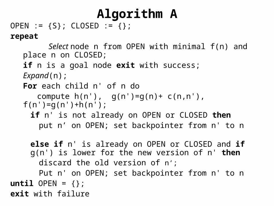
Algorithm AOPEN := {S}; CLOSED := {};repeat Select node n from OPEN with minimal f(n) and place n on CLOSED;

if n is a goal node exit with success;Expand(n);For each child n' of n do compute h(n'), g(n')=g(n)+ c(n,n'), f(n')=g(n')+h(n');

if n' is not already on OPEN or CLOSED thenput n’ on OPEN; set backpointer from n' to n

else if n' is already on OPEN or CLOSED and if g(n') is lower for the new version of n' then

discard the old version of n‘;

Put n' on OPEN; set backpointer from n' to nuntil OPEN = {};exit with failure

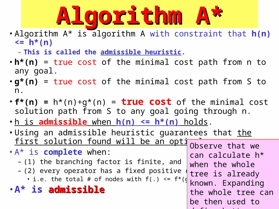
Algorithm A*Algorithm A*• Algorithm A* is algorithm A with constraint that h(n) <= h*(n)

– This is called the admissible heuristic.

• h*(n) = true cost of the minimal cost path from n to any goal. • g*(n) = true cost of the minimal cost path from S to n. • f*(n) = h*(n)+g*(n) = true cost of the minimal cost solution path

from S to any goal going through n.• h is admissible when h(n) <= h*(n) holds.• Using an admissible heuristic guarantees that the first solution

found will be an optimal one. • A* is complete when:

– (1) the branching factor is finite, and– (2) every operator has a fixed positive cost :

• i.e. the total # of nodes with f(.) <= f*(goal) is finite

• A* is admissibleadmissible

Observe that we can calculate h* when the whole tree is already known. Expanding the whole tree can be then used to define better function h.

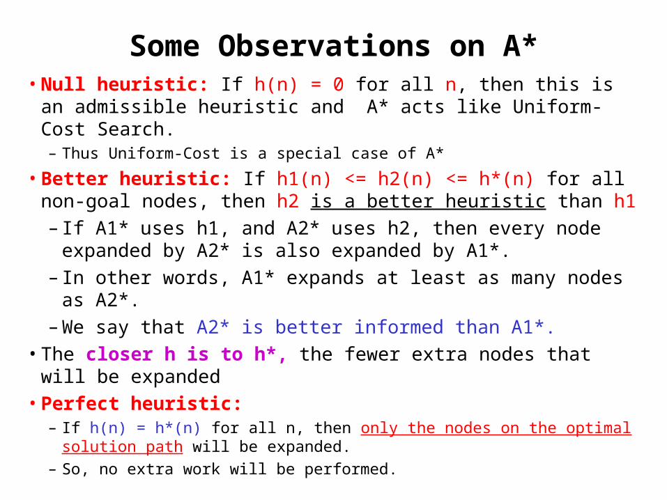
Some Observations on A*• Null heuristic: If h(n) = 0 for all n, then this is an admissible

heuristic and A* acts like Uniform-Cost Search.– Thus Uniform-Cost is a special case of A*

• Better heuristic: If h1(n) <= h2(n) <= h*(n) for all non-goal nodes, then h2 is a better heuristic than h1

– If A1* uses h1, and A2* uses h2, then every node expanded by A2* is also expanded by A1*.

– In other words, A1* expands at least as many nodes as A2*.

– We say that A2* is better informed than A1*.

• The closer h is to h*, the fewer extra nodes that will be expanded

• Perfect heuristic: – If h(n) = h*(n) for all n, then only the nodes on the optimal solution path will

be expanded.

– So, no extra work will be performed.

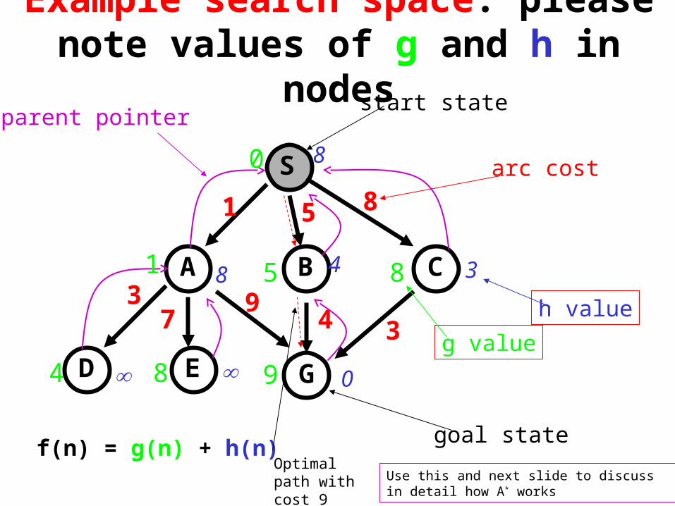
Example search space: please note values of g and h in nodes

S

CBA

D GE

1 5 8

94 3

37

8

8 4 3

0

start state

goal state

arc cost

h value

parent pointer

0

1

4 8 9

85

g value

f(n) = g(n) + h(n)Optimal path with cost 9 Use this and next slide to discuss in detail how A*

works

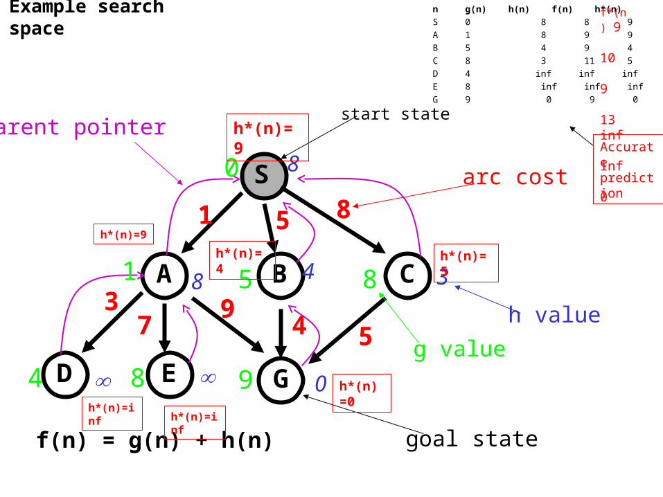
Example search space

S

CBA

D GE

1 5 8

94 5

37

8

8 4 3

0

start state

goal state

arc cost

h value

parent pointer

0

1

4 8 9

85

g value

f(n) = g(n) + h(n)

n g(n) h(n) f(n) h*(n)

S 0 8 8 9

A 1 8 9 9

B 5 4 9 4

C 8 3 11 5

D 4 inf inf inf

E 8 inf inf inf

G 9 0 9 0h*(n)=9

h*(n)=9

h*(n)=4 h*(n)=5

h*(n)=0

h*(n)=infh*(n)=inf

Accurate prediction

f*(n) 9 10 9 13 inf inf 0

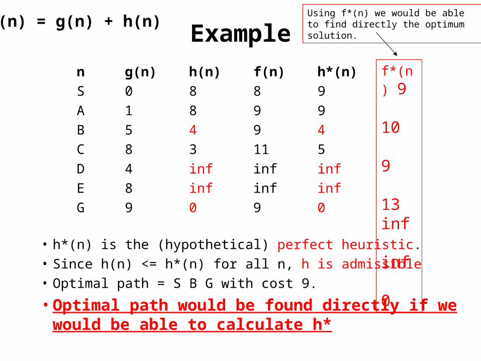
Example

n g(n) h(n) f(n) h*(n)

S 0 8 8 9

A 1 8 9 9

B 5 4 9 4

C 8 3 11 5

D 4 inf inf inf

E 8 inf inf inf

G 9 0 9 0

• h*(n) is the (hypothetical) perfect heuristic.

• Since h(n) <= h*(n) for all n, h is admissible

• Optimal path = S B G with cost 9.

• Optimal path would be found directly if we would be able to calculate h*

f(n) = g(n) + h(n)

f*(n)

9 10 9 13 inf inf 0

Using f*(n) we would be able to find directly the optimum solution.

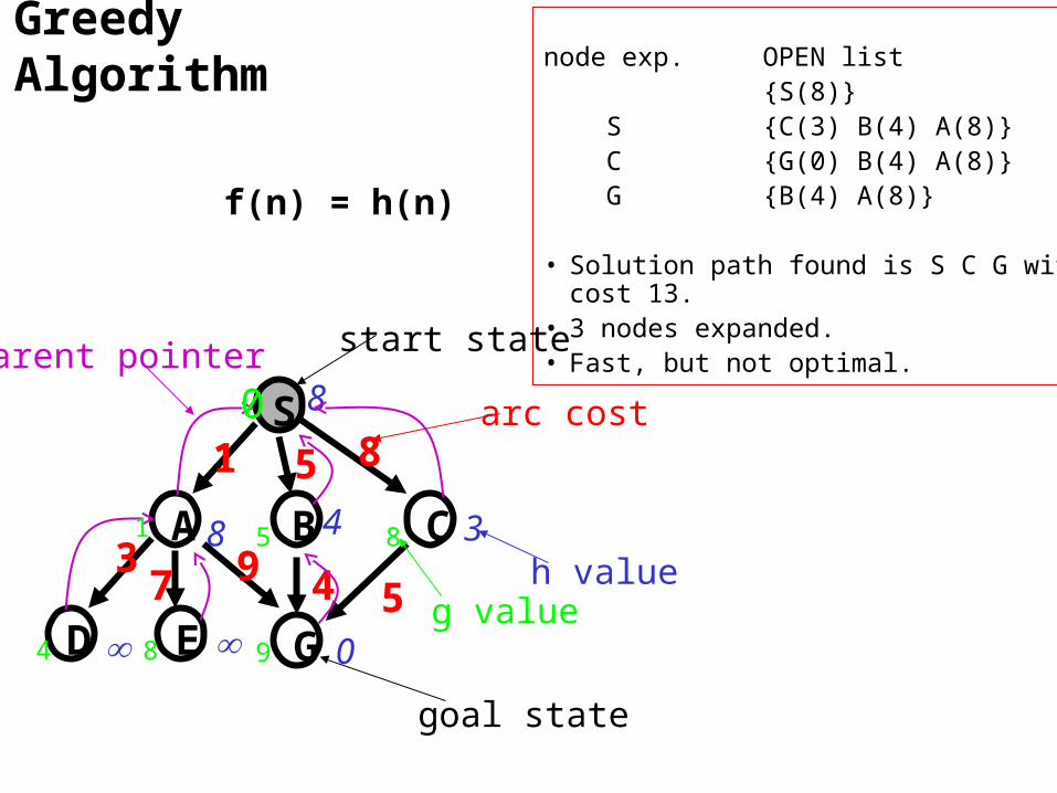
Greedy Algorithm node exp. OPEN list

{S(8)} S {C(3) B(4) A(8)} C {G(0) B(4) A(8)} G {B(4) A(8)}

• Solution path found is S C G with cost 13.• 3 nodes expanded. • Fast, but not optimal.

S

CBA

D GE

1 5 8

9 4 53

7

8

8 4 3

0

start state

goal state

arc cost

h value

parent pointer

0

1

4 8 9

85

g value

f(n) = h(n)

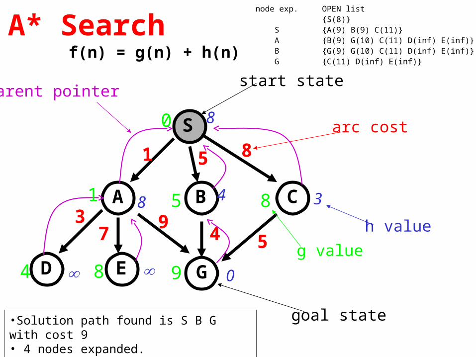
A* Searchnode exp. OPEN list {S(8)} S {A(9) B(9) C(11)} A {B(9) G(10) C(11) D(inf) E(inf)} B {G(9) G(10) C(11) D(inf) E(inf)} G {C(11) D(inf) E(inf)}

S

CBA

D GE

1 5 8

94 5

37

8

8 4 3

0

start state

goal state

arc cost

h value

parent pointer

0

1

4 8 9

85

g value

•Solution path found is S B G with cost 9• 4 nodes expanded.•Still pretty fast. And optimal, too.

f(n) = g(n) + h(n)

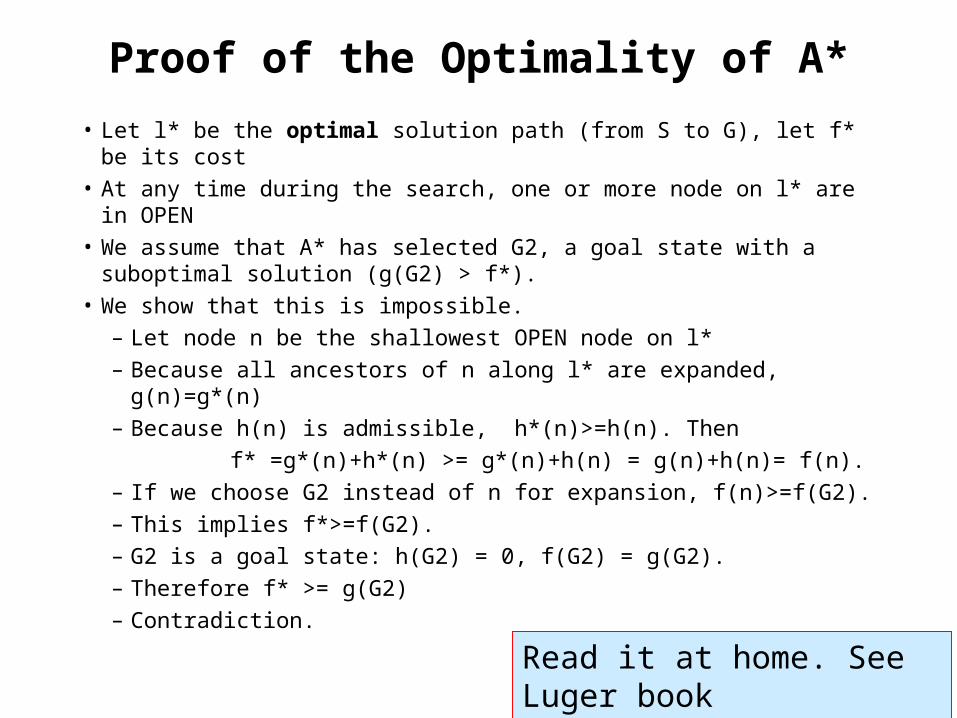
Proof of the Optimality of A*

• Let l* be the optimal solution path (from S to G), let f* be its cost

• At any time during the search, one or more node on l* are in OPEN

• We assume that A* has selected G2, a goal state with a suboptimal solution (g(G2) > f*).

• We show that this is impossible.

– Let node n be the shallowest OPEN node on l*

– Because all ancestors of n along l* are expanded, g(n)=g*(n)

– Because h(n) is admissible, h*(n)>=h(n). Then

f* =g*(n)+h*(n) >= g*(n)+h(n) = g(n)+h(n)= f(n).

– If we choose G2 instead of n for expansion, f(n)>=f(G2).

– This implies f*>=f(G2).

– G2 is a goal state: h(G2) = 0, f(G2) = g(G2).

– Therefore f* >= g(G2)

– Contradiction. Read it at home. See Luger book

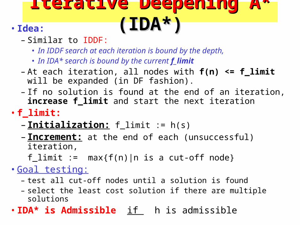
Iterative Deepening A*Iterative Deepening A* (IDA*) (IDA*)• Idea:

– Similar to IDDF:• In IDDF search at each iteration is bound by the depth, • In IDA* search is bound by the current f_limit

– At each iteration, all nodes with f(n) <= f_limit will be expanded (in DF fashion).

– If no solution is found at the end of an iteration, increase f_limit and start the next iteration

• f_limit: – Initialization: f_limit := h(s)– Increment: at the end of each (unsuccessful) iteration,

f_limit := max{f(n)|n is a cut-off node}• Goal testing:

– test all cut-off nodes until a solution is found– select the least cost solution if there are multiple solutions

• IDA* is Admissible if h is admissible

What’s a good heuristic?

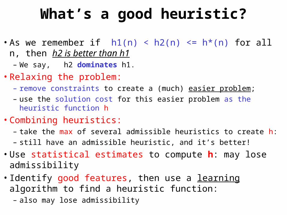
• As we remember if h1(n) < h2(n) <= h*(n) for all n, then h2 is better than h1– We say, h2 dominates h1.

• Relaxing the problem:– remove constraints to create a (much) easier problem;

– use the solution cost for this easier problem as the heuristic function h

• Combining heuristics: – take the max of several admissible heuristics to create h:

– still have an admissible heuristic, and it’s better!

• Use statistical estimates to compute h: may lose admissibility

• Identify good features, then use a learning algorithm to find a heuristic function: – also may lose admissibility

Automatic generation of h functionsAutomatic generation of h functions

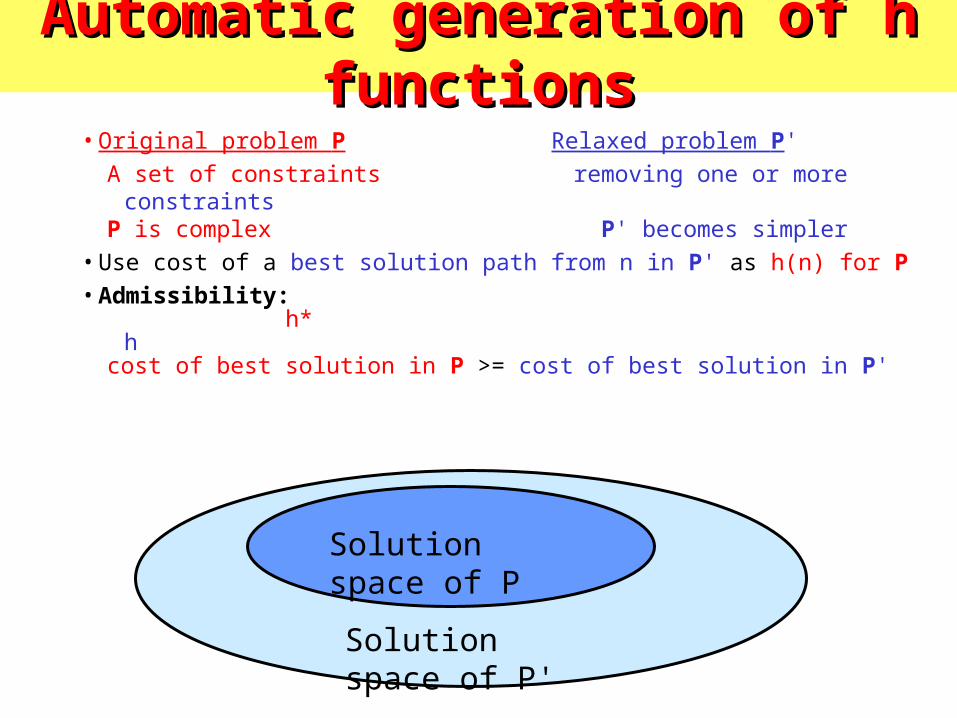
• Original problem P Relaxed problem P'

A set of constraints removing one or more constraintsP is complex P' becomes simpler

• Use cost of a best solution path from n in P' as h(n) for P

• Admissibility: h* hcost of best solution in P >= cost of best solution in P'

Solution space of P

Solution space of P'

Automatic generation of h functions

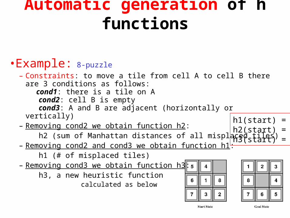
• Example: 8-puzzle

– Constraints: to move a tile from cell A to cell B there are 3 conditions as follows: cond1: there is a tile on A cond2: cell B is empty cond3: A and B are adjacent (horizontally or vertically)

– Removing cond2 we obtain function h2: h2 (sum of Manhattan distances of all misplaced tiles)

– Removing cond2 and cond3 we obtain function h1: h1 (# of misplaced tiles)

– Removing cond3 we obtain function h3: h3, a new heuristic function

calculated as below

h1(start) = 7h2(start) = 18h3(start) = 7

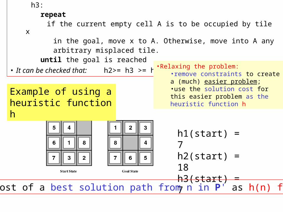
h3: repeat

if the current empty cell A is to be occupied by tile x in the goal, move x to A. Otherwise, move into A any arbitrary misplaced tile. until the goal is reached

• It can be checked that: h2>= h3 >= h1

h1(start) = 7h2(start) = 18h3(start) = 7

•Use cost of a best solution path from n in P' as h(n) for P

•Relaxing the problem:•remove constraints to create a (much) easier problem; •use the solution cost for this easier problem as the heuristic function h

Example of using a heuristic function h

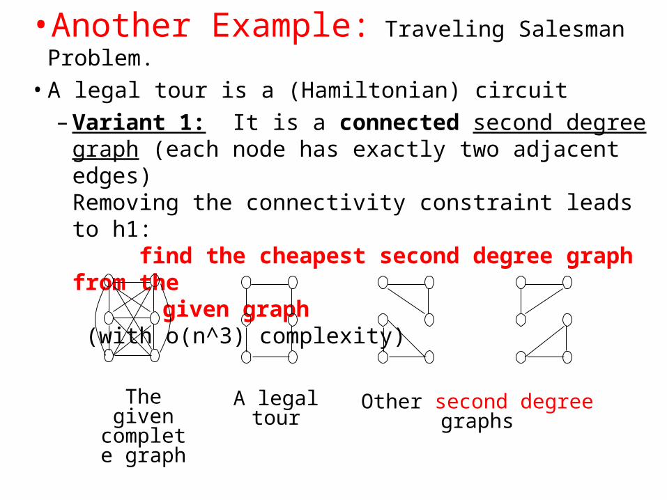
• Another Example: Traveling Salesman Problem.

• A legal tour is a (Hamiltonian) circuit

– Variant 1: It is a connected second degree graph (each node has exactly two adjacent edges)Removing the connectivity constraint leads to h1: find the cheapest second degree graph from the

given graph (with o(n^3) complexity)

The given complete

graph

A legal tour

Other second degree graphs

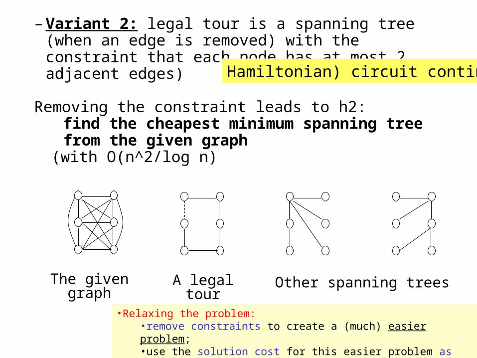
– Variant 2: legal tour is a spanning tree (when an edge is removed) with the constraint that each node has at most 2 adjacent edges)

Removing the constraint leads to h2:find the cheapest minimum spanning tree from the given graph

(with O(n^2/log n)

Other spanning treesThe given graph A legal tour

•Relaxing the problem:•remove constraints to create a (much) easier problem; •use the solution cost for this easier problem as the heuristic function h

Hamiltonian) circuit continued

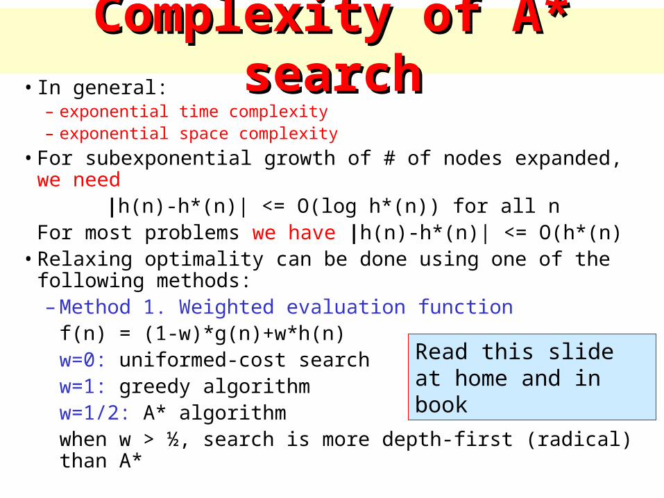
Complexity of A* searchComplexity of A* search• In general:

– exponential time complexity– exponential space complexity

• For subexponential growth of # of nodes expanded, we need|h(n)-h*(n)| <= O(log h*(n)) for all n

For most problems we have |h(n)-h*(n)| <= O(h*(n)• Relaxing optimality can be done using one of the following

methods:– Method 1. Weighted evaluation function

f(n) = (1-w)*g(n)+w*h(n)w=0: uniformed-cost searchw=1: greedy algorithmw=1/2: A* algorithmwhen w > ½, search is more depth-first (radical) than A*

Read this slide at home and in book

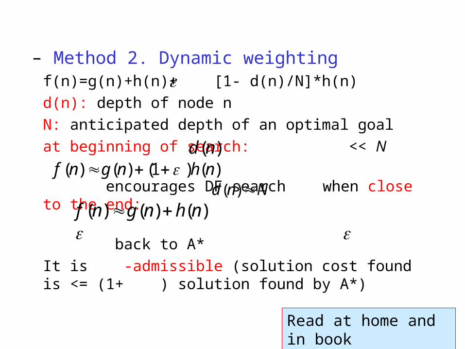
– Method 2. Dynamic weightingf(n)=g(n)+h(n)+ [1- d(n)/N]*h(n)

d(n): depth of node n

N: anticipated depth of an optimal goal

at beginning of search: << N

encourages DF search when close to the end:

back to A*

It is -admissible (solution cost found is <= (1+ ) solution found by A*)

)() 1()()( nhngnf

)()()( nhngnf Nnd )(

)(nd

Read at home and in book

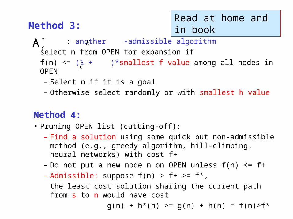
• : another -admissible algorithm

select n from OPEN for expansion if

f(n) <= (1 + )*smallest f value among all nodes in OPEN

– Select n if it is a goal

– Otherwise select randomly or with smallest h value

Method 4:• Pruning OPEN list (cutting-off):

– Find a solution using some quick but non-admissible method (e.g., greedy algorithm, hill-climbing, neural networks) with cost f+

– Do not put a new node n on OPEN unless f(n) <= f+

– Admissible: suppose f(n) > f+ >= f*,

the least cost solution sharing the current path from s to n would have cost

g(n) + h*(n) >= g(n) + h(n) = f(n)>f*

*A

Read at home and in bookMethod 3:

Iterative Improvement SearchIterative Improvement Search

• Another approach to search involves starting with an initial guess at a solution and gradually improving it.

• Some examples:– Hill Climbing

– Simulated Annealing

– Genetic algorithm

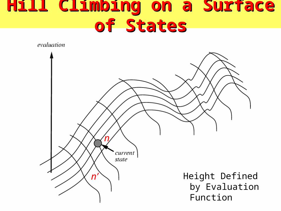
Hill Climbing on a Surface of StatesHill Climbing on a Surface of States

Height Defined by Evaluation Function

n

n’

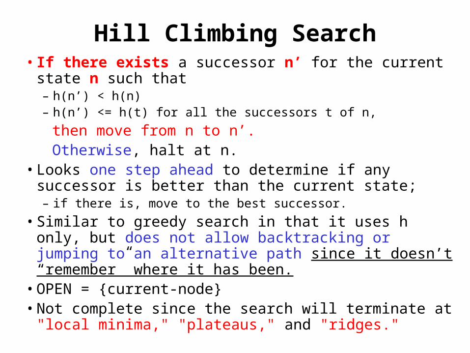
Hill Climbing Search• If there exists a successor n’ for the current state n such that

– h(n’) < h(n)– h(n’) <= h(t) for all the successors t of n,

then move from n to n’. Otherwise, halt at n. • Looks one step ahead to determine if any successor is better than

the current state; – if there is, move to the best successor.

• Similar to greedy search in that it uses h only, but does not allow backtracking or jumping to an alternative path since it doesn’t “remember” where it has been.

• OPEN = {current-node}• Not complete since the search will terminate at "local minima,"

"plateaus," and "ridges."

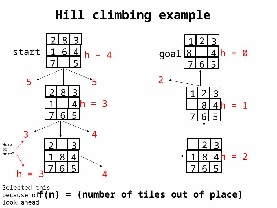
Hill climbing example

2 8 31 6 47 5

2 8 31 47 6 5

2 31 8 47 6 5

1 3 8 47 6 5

2

31 8 47 6 5

2

1 38 47 6 5

2start goal

5

h = 3

h = 3

h = 2

h = 1

h = 0h = 4

5

4

43

2

f(n) = (number of tiles out of place) Selected this because of look ahead

Here or here?

Drawbacks of Hill-Climbing

• Problems:– Local Maxima: – Plateaus: the space has a broad flat plateau with a

singularity as it’s maximum – Ridges: steps to the North, East, South and West

may go down, but a step to the NW may go up.

• Remedy: – Random Restart. – Multiple HC searches from different start states

• Some problems spaces are great for Hill Climbing and others horrible.

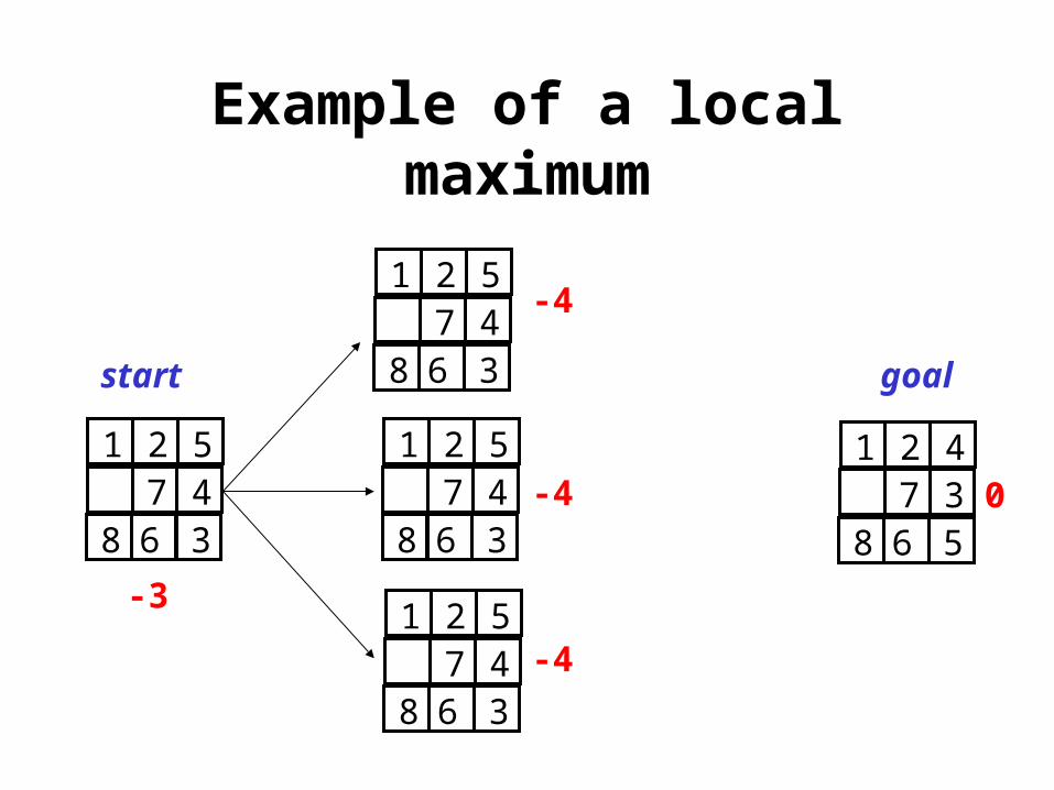
Example of a local maximum

1 2 5 7 48 6 3

1 2 4 7 38 6 5

1 2 5 7 48 6 3

1 2 5 7 48 6 3

1 2 5 7 48 6 3

-3

-4

-4

-4

0

start goal

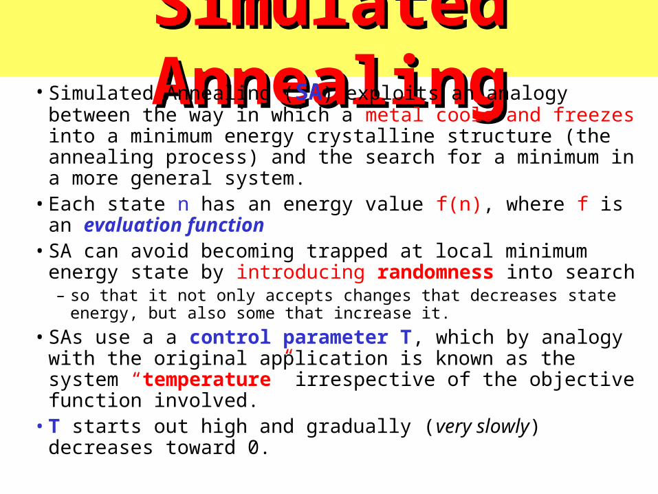
Simulated AnnealingSimulated Annealing• Simulated Annealing (SA) exploits an analogy between the way

in which a metal cools and freezes into a minimum energy crystalline structure (the annealing process) and the search for a minimum in a more general system.

• Each state n has an energy value f(n), where f is an evaluation function

• SA can avoid becoming trapped at local minimum energy state by introducing randomness into search – so that it not only accepts changes that decreases state energy, but also some

that increase it.

• SAs use a a control parameter T, which by analogy with the original application is known as the system “temperature” irrespective of the objective function involved.

• T starts out high and gradually (very slowly) decreases toward 0.

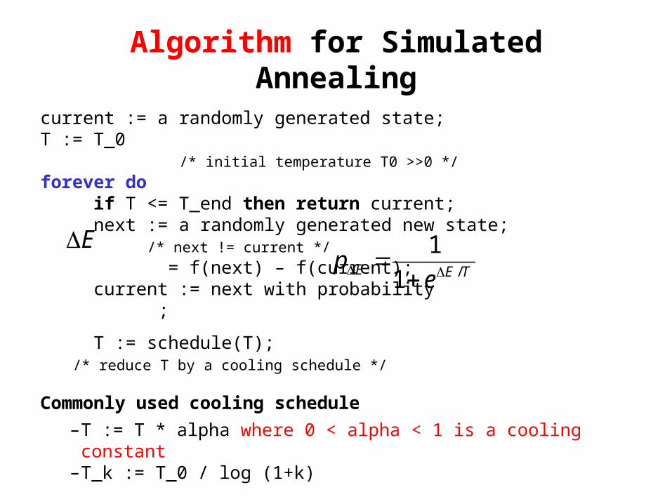
current := a randomly generated state;T := T_0 /* initial temperature T0 >>0 */

forever do if T <= T_end then return current; next := a randomly generated new state; /* next != current */

= f(next) – f(current); current := next with probability ;

T := schedule(T); /* reduce T by a cooling schedule */

Commonly used cooling schedule

– T := T * alpha where 0 < alpha < 1 is a cooling constant– T_k := T_0 / log (1+k)

ETEE e

p/1

1

Algorithm for Simulated Annealing

•

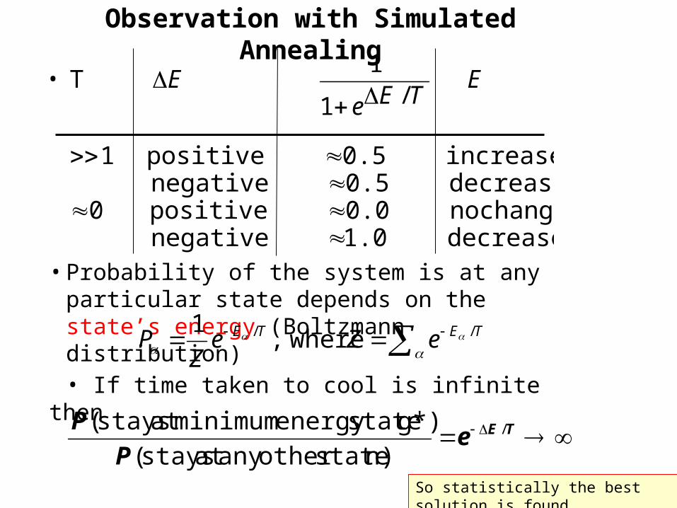
decrease 1.0 negative change no 0.0 positive 0

decrease 0.5 negative increase 0.5 positive 1

/1

1 T

E

TEeE

• Probability of the system is at any particular state depends on the state’s energy (Boltzmann distribution)

• If time taken to cool is infinite then

TETE eZeZ

P // where,1

TEeP

P /

n) stateother any at stays(

g*) stateenergy minimumat stays(

Observation with Simulated Annealing

So statistically the best solution is found

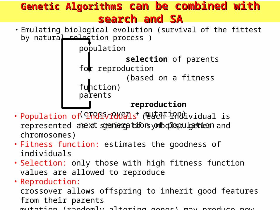
Genetic AlgorithmGenetic Algorithms can be combined with search and SAs can be combined with search and SA

• Emulating biological evolution (survival of the fittest by natural selection process )

• Population of individuals (each individual is represented as a string of symbols: genes and chromosomes)

• Fitness function: estimates the goodness of individuals• Selection: only those with high fitness function values are allowed to reproduce• Reproduction:

crossover allows offspring to inherit good features from their parentsmutation (randomly altering genes) may produce new (hopefully good) featuresbad individuals are throw away when the limit of population size is reached

• To ensure good results, the population size must be large

population

selection of parents for reproduction (based on a fitness function)parents reproduction (cross-over + mutation)

next generation of population

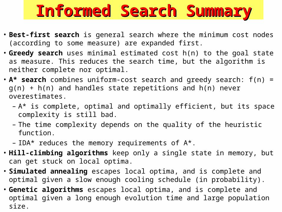
Informed Search SummaryInformed Search Summary• Best-first search is general search where the minimum cost nodes (according to

some measure) are expanded first.

• Greedy search uses minimal estimated cost h(n) to the goal state as measure. This reduces the search time, but the algorithm is neither complete nor optimal.

• A* search combines uniform-cost search and greedy search: f(n) = g(n) + h(n) and handles state repetitions and h(n) never overestimates.

– A* is complete, optimal and optimally efficient, but its space complexity is still bad.

– The time complexity depends on the quality of the heuristic function.

– IDA* reduces the memory requirements of A*.

• Hill-climbing algorithms keep only a single state in memory, but can get stuck on local optima.

• Simulated annealing escapes local optima, and is complete and optimal given a slow enough cooling schedule (in probability).

• Genetic algorithms escapes local optima, and is complete and optimal given a long enough evolution time and large population size.