Instantaneous Squared VIX and VIX Derivatives · Instantaneous Squared VIX and VIX Derivatives Xingguo Luo and Jin E. Zhang† This version: August 22, 2014 Abstract In this paper,

Instantaneous Squared VIX and VIX Derivatives

Xingguo Luo and Jin E. Zhang†

This version: August 22, 2014

Abstract

In this paper, we provide a unified theoretical framework to price VIX derivatives,including futures and options written on both VIX and VXST. Our theory is built onLuo and Zhang’s (2012) concept of instantaneous squared VIX (ISVIX) that is the sum ofinstantaneous Brownian and jump variances of SPX return. Modeling ISVIX as a mean-reverting jump-diffusion process with a stochastic long-term mean, we obtain analyticalformulas for the prices of VIX options and futures. Calibration with the market dataof VIX option implied volatility surface shows that our theory provides an efficient wayof extracting the complete information from VIX derivatives market for the dynamics ofunderlying SPX.

Keywords: VIX; VXST; Instantaneous squared VIX; VIX futures; VIX option

JEL Classification Code: C2; C13; G13;

†Xingguo Luo is from College of Economics and Academy of Financial Research, Zhejiang University,Hangzhou 310027, PR China. Email: [email protected], and Jin E. Zhang is from Department ofAccountancy and Finance, Otago Business School, University of Otago, Dunedin 9054, New Zealand.Email: [email protected].

Instantaneous squared VIX and VIX Derivatives 1

Instantaneous Squared VIX and VIX Derivatives

Abstract

In this paper, we provide a unified theoretical framework to price VIX derivatives,

including futures and options written on both VIX and VXST. Our theory is built on

Luo and Zhang’s (2012) concept of instantaneous squared VIX (ISVIX) that is the sum of

instantaneous Brownian and jump variances of SPX return. Modeling ISVIX as a mean-

reverting jump-diffusion process with a stochastic long-term mean, we obtain analytical

formulas for the prices of VIX options and futures. Calibration with the market data

of VIX option implied volatility surface shows that our theory provides an efficient way

of extracting the complete information from VIX derivatives market for the dynamics of

underlying SPX.

Keywords: VIX; VXST; Instantaneous squared VIX; VIX futures; VIX option

JEL Classification Code: C2; C13; G13


1 Introduction

The VIX options and futures market managed to grow extremely rapidly.1 For example,

the market size of VIX futures and options expand to be an average daily volume 158,580

and 567,460 in 2013 compared with 1,731 and 23,491 in 2006 since their introduction in

2004 and 2006 respectively.2 Recently, on October 1, 2013, the Chicago Board Options Ex-

change (CBOE) introduced the Short-Term Volatility Index (VXST) which is 9-day VIX.3

Subsequently, the CBOE Futures Exchange (CFE) launched VXST futures on February

13, 2014, and the CBOE launched VXST options on April 10, 2014. The new development

of VIX derivatives indicates that the market for volatility trading is highly demanded by

practitioners. It not only generates rich information beyond traditional equity index/stock

derivatives but also pushes an urgent need for cutting-edge academic research on consistent

pricing between VIX and VXST options. However, there is no commonly agreed framework

within which we can both theoretically price VIX derivatives and SPX options simultane-

ously and empirically calibrate model parameters in an efficient way yet, not to mention

study on VXST derivatives.

In this paper, we try to fill this gap by employing Luo and Zhang’s (2012) newly-

developed concept of instantaneous squared VIX (ISVIX), which is the sum of instantaneous

Brownian and jump variances of SPX return.4 Assuming that the ISVIX follows a mean-

reverting jump-diffusion process with a stochastic long-term mean, we are able to derive

analytical formulas for the VIX, VIX futures and options. Further, we use the informative

1Generally, the VIX refers to the 30-day future volatility. In this paper, the VIX includes volatilityindex with any arbitrary time-to-maturity. For simplicity, we denote VIX as the 30-day VIX and specifyexplicitly for VIX with other maturities when necessary.

2Data source: http://www.cboe.com/micro/vix/pricecharts.aspx. For an average VIX value 20, thesevolumes correspond to market values of 3.2 billion and 1.1 billion US dollars. Carr and Lee (2009) providean overview of the market for volatility derivatives including variance swaps and VIX futures and options.

3For more information, please refer to: www.cboe.com/VXST. Note that the S&P 500 three-monthvolatility index under the ticker “VXV” was lunched on November 12, 2007 by the CBOE.

4The jump variance of SPX return is the second term of Equation (3), which is different from varianceswap and will be further clarified when our model is introduced.


VIX term structure data to determine the mean-reverting speed and sequentially calibrate

the volatility and jump parameters in the ISVIX process to market prices of VIX futures

and options.

There is also a fast growing literature on VIX derivatives pricing. Up to now, these

studies can be divided into three groups. The first group starts from classical option pricing

theories in specifying underlying dynamics and derive VIX from the underlying. Due to

fruitful option pricing development, this approach is widely used. In fact, Zhang and Zhu

(2006) is the first study on the VIX futures by considering Heston (1993) model. Zhu and

Zhang (2007) extend Zhang and Zhu (2006) to a model with time-varying long-term mean

of variance. Later on, Lin (2007), Lu and Zhu (2010), Dupoyet, Daigler, and Chen (2011)

and Zhu and Lian (2012) examine more complicated models for VIX futures. Meanwhile,

Sepp (2008a, b), Albanese, Lo and Mijatovi’c (2009), Lin and Chang (2009, 2010)5, Li

(2010), Wang and Daigler (2011), Chung et al (2011), Branger and Volkert (2012), Song

and Xiu (2012), Lian and Zhu (2013), Bardgett, Gourier and Leippold (2013), Chen and

Poon (2013), Lo et al (2013), Romo (2014) and Papanicolaou and Sircar (2014) investigate

various specifications to pricing VIX option. For example, Bardgett, Gourier and Leippold

(2013) conduct a comprehensive analysis by combining time series of SPX, VIX and their

options data and employing an accurate approximation and a powerful filter method in

order to get estimation of totally 23 parameters at one time. They find that a stochastic

central tendency of volatility and jumps in volatility are important in capturing volatility

smiles in both the SPX and VIX markets and tail of variance risk-neutral distribution,

respectively. Papanicolaou and Sircar (2014) propose a regime-switching augmented Hes-

ton model to capture VIX implied volatilities. The second group is more natural in that

it directly model volatility/variance index. For example, Mencia and Sentana (2013) and

5Recently, Cheng et al (2012) prove that Lin and Chang’s (2009, 2010) formula is not an exact solutionof their pricing equation.


Carr and Madan (2013) start from the VIX while Madan and Pistorius (2014) consider

the squared VIX. One drawback of this approach is that the tight link between VIX and

its underlying is not considered and inconsistency may arise in pricing SPX options and

replicating VIX index simultaneously. Bergomi (2008) and Cont and Kokholm (2013) over-

come this drawback by modeling the dynamics of forward variance swap rate, which is

equivalent to the squared VIX. In addition, some studies focus on modeling the dynamics

of underlying volatility/variance, see e.g., Grunbichler and Longstaff (1996), Detemple and

Osakwe (2000). Recently, Goard and Mazur (2013) consider VIX option pricing under

the 3/2-model for underlying volatility. The third group are Huskaj and Nossman (2013)

and Lin (2013), in which they specify exogenous dynamics for the VIX futures. In par-

ticular, Huskaj and Nossman (2013) investigate the normal inverse Gaussian process for

term structure of VIX futures, while Lin (2013) defines a proxy of future VIX as a forward

VIX squared normalized by the VIX futures and studies VIX option by considering various

volatility functions for the proxy.

The purpose of this paper is to provide a unified theoretical framework to price VIX

derivatives, including futures and options written on VIX, VXST and potentially other VIX

with arbitrary time-to-maturity. We demonstrate that analytical formulas of VIX futures

and options can be easily derived with the help of the ISVIX, and parameters can be se-

quentially calibrated by using VIX term structure and VIX option data. Our contributions

are as follows. First, by building on the ISVIX, which is the sum of instantaneous Brow-

nian and jump variances of SPX return, we maintain inherent linkage between SPX and

VIX, thus introduce a consistent method to pricing both SPX option and VIX derivatives.

Second, when modeling ISVIX and leaving underlying dynamics unspecified, we provide

insights into pricing VIX derivatives by focusing on (instantaneous squared) VIX in the

spirit of the second group studies. Calibration with the market data of VIX option implied

volatility surface shows that our theory provides an efficient way of extracting the com-


plete information from VIX derivatives market for the dynamics of underlying SPX. That

is, ISVIX can be used to derive any VIXs with various maturities and estimate parameters

by incorporating all information in VIX term structure, current 30-day VIX options and

even other maturity VIX options that might be developed in the future. Third, we propose

a sequential empirical method to efficiently calibrate parameters by using appropriate mar-

ket data. As emphasized by Bardgett, Gourier and Leippold (2013) that it is important to

combine both SPX and VIX option data to estimate parameters and risk premia. However,

computational burden and difficulty in estimating jumps with short period data challenge

this practice. More importantly, Duan and Yeh (2012) point out that it is crucial to use

the VIX term structure in estimation in order to obtain reliable the risk-neutral volatility

dynamic. In this sense, Bardgett, Gourier and Leippold (2013)’s one-step estimation with-

out the VIX term structure may also suffer from insufficiency. We overcome this obstacle

by proposing a sequential method to estimate parameters with the help of corresponding

market data, which will be discussed in more detail in later section.

Specially, in terms of modelling, a stochastic central tendency is necessary to capture

the dynamics of VIX term structure and it is nontrivial to derive VIX derivatives pric-

ing formula in this setting. It is interesting to note that the importance of modeling

the long-term mean of the variance as the second factor is well recognized in the recent

volatility/variance derivatives literature, though Duffie, Pan and Singleton (2000) mention

a stochastic volatility model with a central tendency and Bates (2000) allows the return

variance to be the sum of the two independent factors which follow square root processes.

For example, Zhang and Huang (2010) study the CBOE S&P 500 three-month variance

futures and suggest that a floating long-term mean level of variance is a good choice for the

variance futures pricing. Zhang, Shu and Brenner (2010) build a two-factor model for VIX

futures, where the long term mean level of variance is treated as a pure Brownian motion.

They find that the model produces good forecasts of the VIX futures prices. Egloff, Leip-


pold and Wu (2010) show that the long-term mean factor is important to capture variance

risk dynamics in variance swap markets.6

The rest of the paper is organized as follows. Section 2 discuss the design of our

model setup. Section 3 derives analytical formulas for VIX futures and options. Section

4 introduces data, calibration procedure and the empirical results. Section 5 provides

concluding remarks.

2 The design of model setup

In this section, we review the concept of ISVIX and main results of Luo and Zhang (2012),

which our theory is built on.

It is an outstanding issue that how to design an efficient setup which can consistently

modeling both SPX and VIX derivatives. The main reason is that the VIX is by construc-

tion a combination of SPX options. We build our model based on following observations.

First, jumps in SPX index and volatility are well documented in the literature. Second,

stochastic long-term mean of volatility is necessary to capture dynamics of volatility term

structure. Third, it is important to derive an intuitive formula for VIX and sperate in-

formation in different markets in order to reduce computational burden in estimation. To

deal with these concerns, we employ the model proposed by Luo and Zhang (2012), that

is the following model for the SPX index, St, under the risk-neutral measure Q,

dSt/St− = rdt+√vtdB

Q1,t + (ex − 1)dNx

t − λxtEQ(ex − 1)dt,

Vt ≡ vt + 2λxtEQ(ex − 1− x),

dVt = κ(θt − Vt)dt+ σV√

VtdBQ2,t + ydNy

t − λyEQ(y)dt,

dθt = σθdBQ3,t

(1)

6While Adrian and Rosenberg (2008) and Christoffersen, Jacobs, Ornthanalai, and Wang (2008) inves-tigate long-run and short-run volatility components, Christoffersen, Heston and Jacobs (2009) consider thetwo-factor square root process.


where r is the risk-free rate, BQ1,t and B

Q2,t are two related Brownian motions. Nx

t is a pure

jump processes with jump size x and jump intensity λxt . κ is the mean-reverting speeds of

Vt. θt is the long-term mean level of Vt. Nyt is another pure jump processes with jump size

y and jump intensity λy and BQ3,t is another Brownian motion which is independent of BQ

1,t

and BQ2,t.

7

Then, the concept of instantaneous squared VIX can be introduced, that is,

Definition 1 (Luo and Zhang, 2012) For the jump-diffusion model specified in (1), the

instantaneous squared VIX (ISVIX), Vt, is given by

Vt ≡ limτ→0

2

τEQt

[∫ t+τ

t

dSuSu

− d(lnSu)

]

, (2)

= vt + 2λtEQ(ex − 1− x). (3)

From (2), we can see that the ISVIX is the limit of squared V IX when maturity approaches

zero. Because of the martingale specification for innovation parts in the dynamics of Vt,

we can obtain an intuitive formula for the squared VIX, that is,

Proposition 1 (Luo and Zhang, 2012) Under the previous jump-diffusion model, the

squared VIX, at time t, with maturity τ0, V IX2t,τ0

, can be expressed as

V IX2t,τ0

= ωVt + (1− ω)θt, (4)

where

ω ≡ ω(τ0) =1− e−κτ0

κτ0. (5)

Remark 1 τ0 can be arbitrary time-to-maturity. Particularly, τ0 = 30365

and τ0 = 9365

correspond to the VIX and VXST respectively.

7At this point, we use constant jump intensity and martingale long-term mean to demonstrate ourmodel, they can be relaxed very easily, but we do not want move too far as we want our model to besimple, yet useful.


3 Theory of VIX option pricing

In this section, we derive conditional probability density function of VIX and analytical

formulas for VIX options and futures. Also, to illustrate accuracy of current model, we

compare our VIX futures formula with the exact one studied in Zhang and Zhu (2006) for

the Heston model. Further, we investigate sensitivity of VIX option implied volatility with

respect to the parameters.

3.1 Conditional probability density function of VIX

For the VIX derivatives pricing, the key is to derive the joint moment generating function

of (VT , θT ) conditional upon current observable variables (Vt, θt).

Lemma 1 Under the previous jump-diffusion model, the conditional probability density

function of V IXT , p(V IXT |V IXt), is given by

p(V IXT |V IXt) =2V IXT

π

∫ ∞

0

Re[

e−iφV IX2

T f(iφ; t, τ, Vt, θt)]

dφR, (6)

where φ = φR + φIi is a complex variable and f(φ; t, τ, Vt, θt) is the moment generating

function of V IX2T , which is given by

f(φ; t, τ, Vt, θt) = EQ[eφV IX2

T |Ft],

= EQ[eφωVT+φ(1−ω)θT |Ft],

= f(φω, φ(1− ω); t, τ, Vt, θt), (7)

where f(φ, ψ; t, τ, Vt, θt) is the moment generating function of (VT , θT ) in the following

f(φ, ψ; t, τ, Vt, θt) = eA1(φ,ψ;τ)+A2(φ,ψ;τ)Vt+A3(φ,ψ;τ)θt+A4(φ,ψ;τ), (8)


where

A1(φ, ψ; τ) =−λyEQ(y)

κ(A3(φ, ψ; τ)− ψ) +

1

2σ2θ

∫ τ

0

A23(φ, ψ; u)du, (9)

A2(φ, ψ; τ) =2κφ

(2κ− σ2V φ)e

κτ + σ2V φ

, (10)

A3(φ, ψ; τ) = ψ − 2κ

σ2V

ln

[

1 +σ2V φ

2κ(e−κτ − 1)

]

, (11)

A4(φ, ψ; τ) =

∫ τ

0

λyEQ[eA2(φ,ψ;u)y − 1]du. (12)

See Appendix A for proof.

Further, the characteristic function of V IX2T is given by f(iφ; t, τ, Vt, θt) and the cor-

responding conditional density function of V IX2T , p(V IX

2T |V IX2

t ), is the (generalized)

Fourier inversion of the characteristic function

p(V IX2T |V IX2

t ) =1

π

∫ ∞

0

Re[

e−iφV IX2


dφR, (13)

3.2 VIX options and futures

The price of a European VIX call option, c(t, T ), at time t with maturity T and strike K

is

c(t, T ) = e−r(T−t)EQ[(V IXT −K)+|Ft],

= e−r(T−t)∫ ∞

0

p(V IXT |V IXt)(V IXT −K)+dV IXT ,

=e−rτ

π

∫ ∞

0

2V IXT

∫ ∞

0

Re[

e−iφV IX2


dφR(V IXT −K)+dV IXT .

(14)

Because Lewis (2000) and Poularikas (2000) derive

∫ ∞

0

e−ξz(√z −K)+dz =

√π

2

1− erf(K√ξ)

(√ξ)3

, (15)


where ξ is a complex Fourier transform variable with Re[ξ] > 0, and erf(u) is a complex

error function given by erf(u) = 2√π

∫ u

0e−v

2

dv, we have

I1 =

∫ ∞

0

2V IXT e−iφV IX2

T (V IXT −K)+dV IXT ,

=

∫ ∞

0

e−iφV IX2

T (V IXT −K)+dV IX2T ,

=

√π

2

1− erf(

K√iφ)

(√iφ)3

, φI < 0. (16)

Proposition 2 Therefore, the call option price becomes

c(t, T ) =e−rτ

π

∫ ∞

0

Re[

I1 · f(iφ; t, τ, Vt, θt)]

dφR,

=e−rτ

2√π

∫ ∞

0

Re

[

1− erf(

K√iφ)

(√iφ)3

f(iφ; t, τ, Vt, θt)

]

dφR, φI < 0. (17)

Remark 2 It is important to note that the ω is a function of τ0, and Equation (17) can

be applied to any τ0. Thus, it provides a unified platform for us to study the consistency

between options written on VIX, VXST and VIX with other maturities.

Remark 3 Lian and Zhu (2013) use similar methodology and derive a VIX option

formula for a one-factor stochastic volatility model with simultaneous jumps in both index

return and volatility process. However, our formula in (17) is based on a general two-factor

stochastic volatility model with a time-varying central tendency θt. Further, we derive VIX

option formula by using a simple relation between VIX and Vt and θt in (4), which enable

us to obtain the two latent factors from observable VIX term structure data.

Corollary 1 The VIX futures price can also be calculated from VIX option formula, that

is

F (t, T ) =1

2√π

∫ ∞

0

Re

[

1

(√iφ)3

f(iφ; t, τ, Vt, θt)

]

dφR, φI < 0. (18)


Remark 4 In the following sections, we consider a special case, y ∼ exp(µy), to get

closed-form solution for A4(φ, ψ; τ). We have

A4(φ, ψ; τ) =2λyµy

2κµy − σ2V

ln

[

1 +(σ2

V − 2µyκ)φ

2κ(1− µyφ)(e−κτ − 1)

]

. (19)

3.3 Property of the VIX futures and option pricing formulas

We discuss property of VIX futures and option pricing formulas in more detail in this

section.

3.3.1 Comparison with Zhang and Zhu (2006)

First, we compare current VIX futures formula with the exact density function in the

Heston model. In this case, we have λxt = λy = 0, Vt = vt and θt = θ. To compare with

the exact transit density function, we just compare it to the density function in our model.

Now, the moment generating function of VT becomes

f1(φ; t, τ, Vt) ≡ EQ[eφVT |Ft], (20)

= eA1(φ;τ)+A2(φ;τ)Vt , (21)

with

A1(φ; τ) =−2κθ

σ2V

ln

[

1 +σ2V φ

2κ(e−κτ − 1)

]

, (22)

A2(φ; τ) =2κφ

(2κ− σ2V φ)e

κτ + σ2V φ

. (23)

The corresponding conditional density function of VT , p1(VT |Vt), is

p1(VT |Vt) =1

π

∫ ∞

0

Re[

e−iφVT f1(iφ; t, τ, Vt, θt)]

dφR. (24)

Then, the VIX futures price is given by

F1(t, T ) =1

2√π

∫ ∞

0

Re

[

1

(√iφ)3

eφ(1−ω)θf1(φω; t, τ, Vt)

]

dφR. (25)


Table 1 provides comparison for VIX futures with maturities 15, 78, 169 and 260 days

on March 1, 2005. Note that the physical measure parameters used in Zhang and Zhu

(2006) are κP = 5.7895, θP = 0.0414, σV = 0.4868 and the volatility risk premium is

λ = −0.8716. In current VIX futures formula, we need to use risk-neutral parameters

given by κ = κP + λ, θ = κP θP

κP+λ. In addition, the VIX level on March 1, 2005 is 12.04,

which can be used to back out Vt = 0.0071. Table 1 shows that VIX futures prices are the

same by using current VIX futures formula in (25) and the exact formula in Zhang and

Zhu (2006).

3.3.2 Sensitivity of VIX option implied volatility

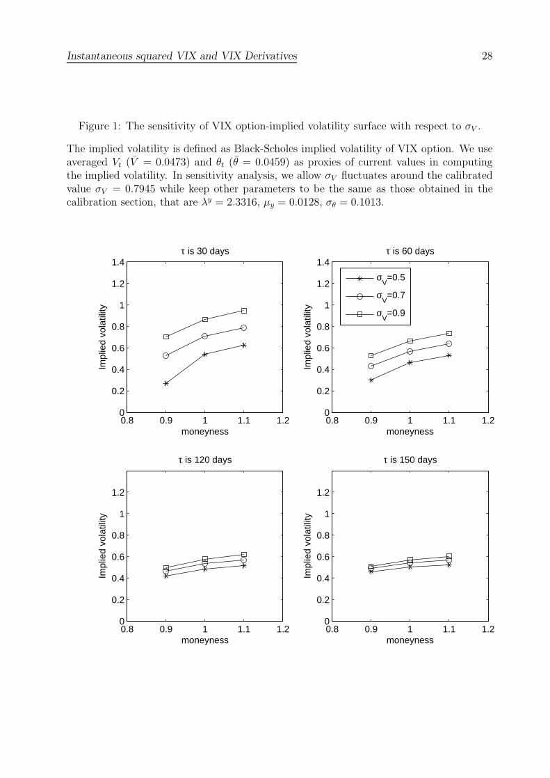
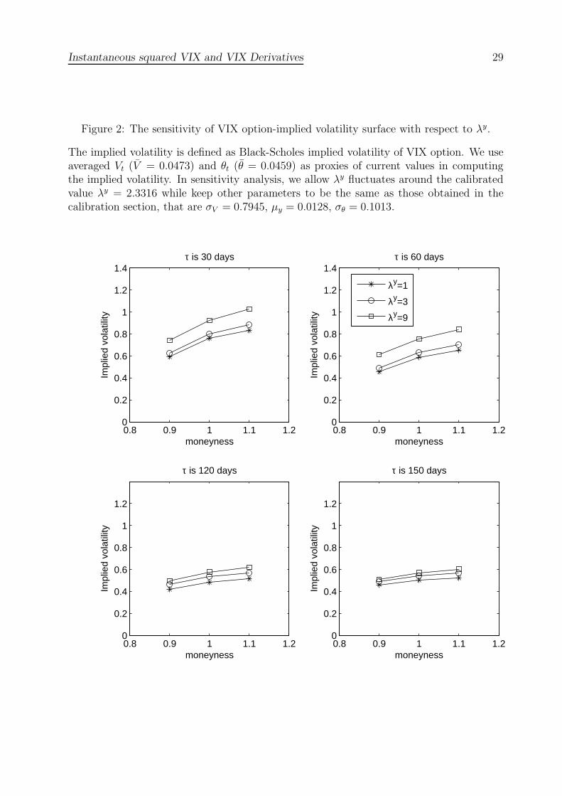
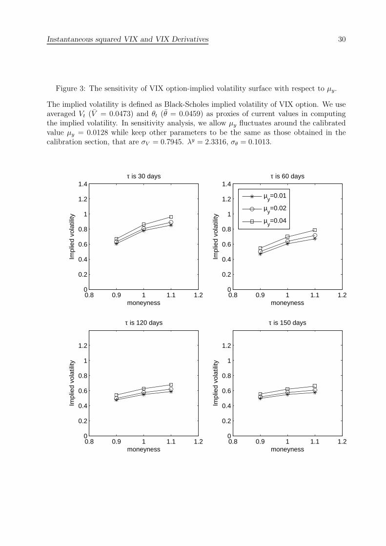
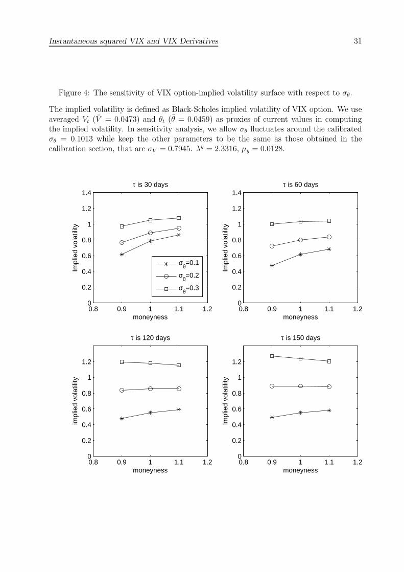
To guide parameter calibration in the next section, we conduct sensitivity analysis of VIX

option implied volatility with respect to the four parameters, σV , λy, µy and σθ, for various

combinations of maturity and moneyness. Figures 1-4 show the results.

When look vertically in the up-left part of Figure 1, we can see that implied volatility

is sensitive to different values of σV and larger σV corresponds to higher implied volatility.

The difference becomes less when moneyness goes up. Further, implied volatility curve is a

increasing function of moneyness. When maturity increases to 60, 120 and 150 days, we find

that the implied volatility curve becomes more and more flat and the difference caused by

different σV becomes smaller. We observe similar pattern in Figures 2-3. However, Figure 4

indicates that the difference induced by different σθ becomes larger when maturity increases.

Moreover, the implied volatility curve switches from upward sloping to downward sloping

function of moneyness.

4 Calibration

In this section, we introduce data and calibrate the model to the average VIX futures term

structure, ATM implied volatility term structure and implied volatility skew term structure


with maturities 30, 60, 90, 120 and 150 days. By minimizing squared errors, we are able

to get solutions of σV , λy, µy and σθ.

4.1 Data

The daily market data employed in this paper includes VIX futures from March 26, 2004

to May 28, 2010 and options from February 24, 2006 to May 28, 2010 provided by the

CBOE. The VIX futures data contains trading date and maturity date; open, high, low

and close of the futures price; settle price, which is used as the proxy of futures price on

the trading date; trading volume and open interest. On each trading day, we calculate VIX

futures prices with the standardized times-to-maturity of 30, 60, 90, 120 and 150 days by

using linear interpolation. We treat VIX index as the VIX futures price with zero day to

maturity. Table 2 provides descriptive statistics of VIX futures data. The VIX options

data contains trading date and expiration date; type of options (call or put) and strike

price; open, high, low and close prices; trading volume and open interests; last bid and last

ask prices; underlying VIX index values. For each VIX options contract, last traded prices

of VIX options are often unavailable, and reported last traded prices are often zero in the

original dataset. We therefore use mid-price of closing bid and ask as the closing price of

the options.

We notice that the expiration dates in the original VIX options dataset are not the

true expiration dates. They are the third or fourth Saturdays of the months, while the

VIX options expiration dates are Wednesdays. Therefore we need to transfer the original

expiration dates to true expiration dates before we start to process the data. For example,

if the original expiration dates are March 18, 2006 and April 22, 2006, we first find the

third Friday in the next month of the original expiration dates, which are April 21, 2006

and May 19, 2006. We then subtract 30 days from these “third Fridays in the next month”

and obtain some Wednesdays in the original months, and these Wednesdays, such as March


22, 2006 and April 19, 2006 for the example, are the true expiration dates. We obtain the

days to maturity by calculating the number of calendar days between the trading date and

the true expiration date, and we then divide it by 365 to annualize the time to maturity.

For example, if the trading date is March 1, 2006, and true expiration dates are March 22,

2006 and April 19, 2006, then the days to maturity are 21 days and 49 days, and annualized

time to maturity are 0.0575 and 0.1342 year.

We also use U.S. treasury daily yield curve rates during the same period above, provided

by the U.S. Treasury Department. The U.S. treasury daily yield curve rates include treasury

yields for 1 month, 3 months, 6 months, 1 year, 2 years, 3 years, 5 years, 7 years, 10 years, 20

years, and 30 years, on each trading day. We construct risk-free interest rates for different

maturities on each trading day by using linear interpolation.

4.1.1 ATM implied volatility

Before calculating ATM implied volatility, we first introduce implied forward price and

ATM implied forward price. The implied forward price is computed from the options

market by using put-call parity, i.e.,

ct(K)− pt(K) = St −Ke−r(T−t). (26)

The forward price at time t with maturity T is given by

Fimplied(K) = Ster(T−t) = (ct(K)− pt(K))er(T−t) +K. (27)

Notice that the implied forward price could be a function of strike price K. We define the

pair of call and put options with the same strike and the smallest absolute value of the

price difference as the ATM options. The implied forward price computed from the pair of

ATM call and put is called ATM implied forward price.

The implied volatility of an option is defined as the volatility that equates the Black-


Scholes option price with the market price of the option, i.e.,

cMarkett (K, T − t) = cBlack−Scholest (σ;K, T − t) = F T

t e−r(T−t)N(d1)−Ke−r(T−t)N(d2), (28)

where F Tt is the ATM implied forward price and

d1 =ln

FTt

K+ 1

2σ2(T − t)

σ√T − t

, d2 = d1 − σ√T − t. (29)

The ATM implied volatility is regarded as the implied volatility for the option with strike

price being equal to the ATM implied forward price, i.e., K = F Tt . We look for two strike

prices, Klower and Kupper, that are the nearest strike below and above the ATM implied

forward price, and then calculate the ATM implied volatility by using linear interpolation

with the implied volatilities at these two strike prices.

4.1.2 ATM implied volatility skew

On each trading day, for the VIX options with the same maturity, the implied volatility

skew is defined as the ATM slope of the implied volatility as a function of strike price, that

is

skew =σimplied(Kupper)− σimplied(Klower)

Kupper −Klower

. (30)

We can calculate daily ATM implied volatility and ATM implied volatility skew over

the sample period for maturities 30, 60, 90, 120 and 150 days. The average ATM implied

volatility term structure and average ATM implied volatility skew term structure are means

of corresponding daily values. That is, the average ATM implied volatility term structure

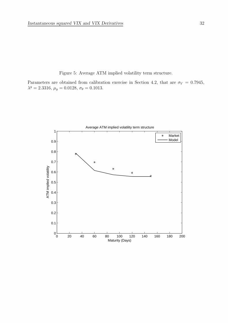
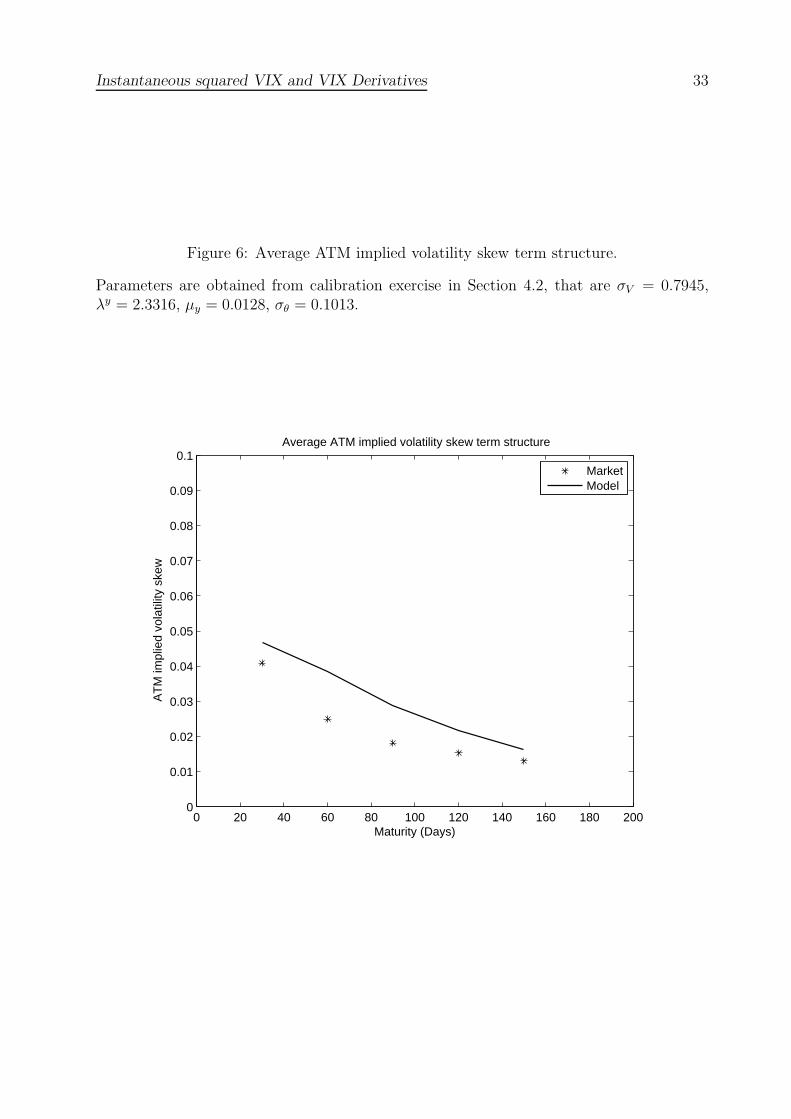
are 0.7764, 0.695, 0.6312, 0.5923, 0.5612, and the average ATM implied volatility skew term

structure are 0.0409, 0.0249, 0.0182, 0.0154, 0.0131.

4.2 Calibration

We do calibration in two steps. First, we use VIX term structure daily data from January

2, 1992 to May 28, 2010 to estimate parameter set {κ, Vt, θt}t=1,...,T over the sample period.


We employ an efficient procedure in Luo and Zhang (2012) and obtain κ = 5.5282. We

average Vt and θt to get V = 0.0473 and θ = 0.0459. Second, we obtain σV = 0.7945,

λy = 2.3316, µy = 0.0128 and σθ = 0.1013 by solving the following minimization problem

{σV , λy, µy, σθ} = argmin

5∑

j=1

(

IVj − IV Mktj

IV

)2

+

(

Skewj − SkewMktj

Skew

)2

, (31)

where j = 1, ..., 5 indicate 30, 60, 90, 120 and 150 days, IVj is averaged model-implied ATM

implied volatility, Skewj is averaged model-implied ATM implied volatility skew, IV Mktj

and SkewMktj are corresponding market-implied values, and IV and Skew are the mean of

IV Mktj and SkewMkt

j respectively.

Table 3 provides pricing errors of VIX futures. Note that we consider subsample period

and full sample period in Panels A and B, respectively. It can be seen that pricing errors

are small for both sample periods.

Figures 5-7 show fitting performance of current VIX futures and options formulas by

using estimated parameters. In particular, Figure 5 shows that model-implied average ATM

implied volatility term structure is similar to market data. Further, Figure 6 means that

our model can also track the shape of average ATM implied volatility skew term structure.

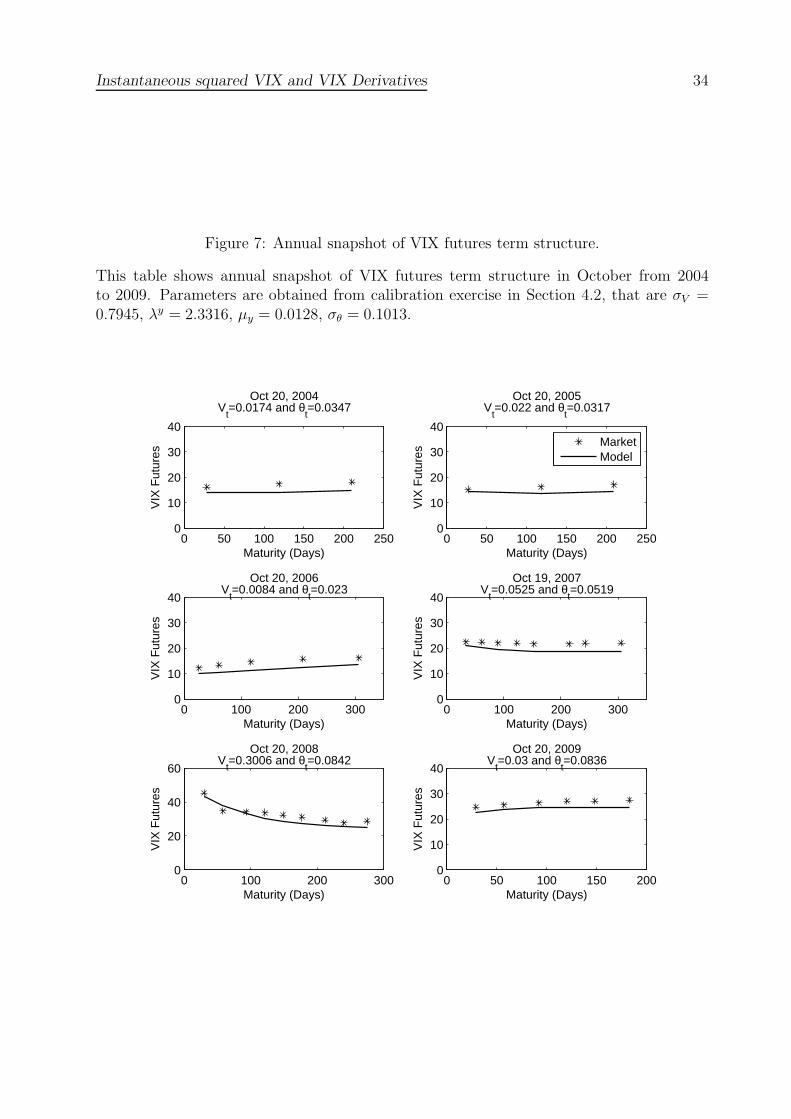
Figure 7 plots six annual snapshot of VIX futures term structure from 2004 to 2009. It is

clear that theoretical VIX futures values closely match market data and capture various

shapes of VIX term structure at both low and high levels of volatility market conditions.

5 Concluding remarks

In this paper, we introduce a unified framework to price VIX derivatives, which includes

futures and options written on VIX, VXST and VIX with any other maturity, by using

the instantaneous squared VIX proposed in Luo and Zhang (2012). We also show that

parameters can be efficiently estimated by a sequential method. It turns out that our


model is simple yet powerful to capture various shapes of VIX futures term structure and

fit term structures of average ATM implied volatility and its skew.

Note that, we do not compare different specifications and investigate their relative

contributions. Instead, we focus on pointing out the importance of the ISVIX in pricing

derivatives on VIX with various maturities in a unified model, and bridging the SPX and

VIX derivatives markets. We demonstrate that analytical formulas for VIX options and

futures can be obtained in a mean-reverting jump-diffusion process with a stochastic long-

term mean. Further, we propose a sequential estimation method by using appropriate

market information to determine relevant parameters. That is, VIX term structure data

can be used to estimate the mean-reverting speed and VIX option implied volatility surface

is employed to calibrate the volatility and jump parameters. By doing this, we actually

decompose a complicated estimation task into several simpler tasks.

At last, it is worthwhile to mention that how to specify instantaneous Brownian variance

and jump dynamics of SPX return, how to estimate these parameters by combining SPX

options, and how to further extend ISVIX dynamics are important issues can be considered.

Nevertheless, we leave them for future research.


A Solution of f(φ, ψ; t, τ, Vt, θt)

Let τ ≡ T − t and

f(φ, ψ; t, τ, Vt, θt) ≡ EQ[eφVT+ψθT |Ft], (32)

be the joint moment generating function of (VT , θT ). Since f(φ, ψ; t, τ, Vt, θt) is a martingale,

it satisfies backwards Kolmogorov equation

−fτ + [κ(θt−Vt)− λyEQ(y)]fV +1

2σ2V V fV V +

1

2σ2θfθθ + λyEQ[f(V + y)− f(V )] = 0, (33)

with a boundary condition f(φ, ψ; t + τ, 0, Vt, θt) = eφVT+ψθT . Assume a solution of with

the following form

f(φ, ψ; t, τ, Vt, θt) = eA1(φ,ψ;τ)+A2(φ,ψ;τ)Vt+A3(φ,ψ;τ)θt+A4(φ,ψ;τ), (34)

with the boundary conditionsA1(φ, ψ; 0) = A4(φ, ψ; 0) = 0, A2(φ, ψ; 0) = φ andA3(φ, ψ; 0) =

ψ. Substituting the derivatives to the above PIDE, we have

−[

A′

1(τ) + A′

2(τ)Vt + A′

3(τ)θt + A′

4(τ)]

+ [κ(θt − Vt)− λyEQ(y)]A2(τ) +1

2σ2VA

22(τ)Vt

+1

2σ2θA

23(τ) + λyEQ[eA2(τ)y − 1] = 0.

(35)

We have the following ODEs

A′

1(τ) = −λyEQ(y)A2(τ) +1

2σ2θA

23(τ),

A′

2(τ) = −κA2(τ) +1

2σ2VA

22(τ),

A′

3(τ) = κA2(τ),

A′

4(τ) = λyEQ[eA2(τ)y − 1].

We first solve Riccati equation of B(τ) and obtain

A2(φ, ψ; τ) =2κφ

(2κ− σ2V φ)e

κτ + σ2V φ

. (36)


Then, A3(τ) and A4(τ) can be calculated as

A3(φ, ψ; τ) = ψ − 2κ

σ2V

ln

[

(1− σ2V φ

2κ) +

σ2V φ

2κe−κτ

]

, (37)

A4(φ, ψ; τ) =

∫ τ

0

λyEQ[eA2(u)y − 1]du, (38)

and A1(τ) is given by

A1(φ, ψ; τ) = −λyEQ(y)

∫ τ

0

A2(u)du+1

2σ2θ

∫ τ

0

A23(u)du,

=−λyEQ(y)

κ(A3(τ)− ψ) +

1

2σ2θ

∫ τ

0

A23(u)du.

(39)


References

[1] Adrian, Tobias, and Joshua Rosenberg, 2008, Stock returns and volatility: Pricing the

short-run and long-run components of market risk, Journal of Finance 63, 2997-3030.

[2] Albanese, C., H. Lo, and A. Mijatovic, 2009, Spectral methods for volatility derivatives,

Quantitative Finance 9(6), 663-692.

[3] Bardgett, Chris, Elise Gourier, and Markus Leippold, 2013, Inferring volatility dy-

namics and risk premia from the S&P 500 and VIX markets, Working paper, Swiss

Finance Institute.

[4] Bates, David S., 2000, Post-87 crash fears in S&P 500 futures options, Journal of

Econometrics 94, 181-238.

[5] Bergomi, L., 2008, Smile dynamics III, Risk 21, 90-96.

[6] Branger, Nicole, and Clemens Volkert, 2012, The fine structure of variance: Consistent

pricing of VIX derivatives. Working paper, Univeristy of Munster.

[7] Carr, Peter, and Roger Lee, 2009, Volatility derivatives, Annual Review of Financial

Economics 1, 1-21.

[8] Carr, Peter, and Dilip B. Madan, 2013, Joint modeling of VIX and SPX options at a

single and common maturity with risk management applications, Working paper, New

York University.

[9] Chen, Ke, and Ser-Huang Poon, 2013, Consistent pricing and hedging volatility deriva-

tives with two volatility surfaces, Working paper, University of Manchester.


[10] Cheng, Jun, Meriton Ibraimi, Markus Leippold and Jin E. Zhang, 2012, A remark

on Lin and Chang’s paper “Consistent modeling of S&P 500 and VIX derivatives”,

Journal of Economic Dynamics and Control 36(5), 708-715.

[11] Christoffersen, Peter F., Steven Heston, and Kris Jacobs, 2009, The shape and term

structure of the index option smirk: Why multifactor stochastic volatility models work

so well, Management Science 55, 1914-1932.

[12] Christoffersen, Peter F., Kris Jacobs, Chayawat Ornthanalai, and Yintian Wang, 2008,

Option valuation with long-run and short-run volatility components, Journal of Fi-

nancial Economics 90, 272-297.

[13] Chung, S.-L., W.-C. Tsai, Y.-H. Wang, and P.-S. Weng, 2011, The information content

of the S&P 500 index and VIX options on the dynamics of the S&P 500 index, Journal

of Futures Markets 31(12), 1170-1201.

[14] Cont, R., and T. Kokholm, 2013, A consistent pricing model for index options and

volatility derivatives, Mathematical Finance 23, 248-274.

[15] Detemple, J., and C. Osakwe, 2000, The valuation of volatility options, European

Finance Review 4, 21-50.

[16] Duan, Jin-Chuan, and Chung-Ying Yeh, 2010, Jump and volatility risk premiums

implied by VIX, Journal of Economic Dynamics and Control 34, 2232-2244.

[17] Duan, Jin-Chuan, and Chung-Ying Yeh, 2012, Price and volatility dynamics implied

by the VIX term structure, Working paper, National University of Singapore.

[18] Duffie, D., J. Pan, and K. J. Singleton, 2000, Transform analysis and asset pricing for

affine jump-diffusion, Econometrica 68, 1343-1376.


[19] Dupoyet, Brice, Robert T. Daigler, and Zhiyao Chen, 2011, A simplified pricing model

for volatility futures, Journal of Futures Markets 31, 307-339.

[20] Egloff, Daniel, Markus Leippold, and Liuren Wu, 2010, The term structure of vari-

ance swap rates and optimal variance swap investments, Journal of Financial and

Quantitative Analysis 45, 1279-1310.

[21] Goard, Joanna, and Mathew Mazur, 2013, Stochastic volatility models and the pricing

of VIX options, Mathematical Finance 23, 439-458.

[22] Grunbichler, A., and F. Longstaff, 1996, Valuing futures and options on volatility,

Journal of Banking and Finance 20, 985-1001.

[23] Heston, Steven L., 1993, A closed-form solution for options with stochastic volatility

with applications to bond and currency options, Review of Financial Studies 6, 327-

343.

[24] Huskaj, Bujar, and Marcus Nossman, 2013, A term structure model for VIX futures,

Journal of Futures Markets 33, 421-442.

[25] Lewis, A., 2000, Option Valuation Under Stochastic Volatility, Finance Press, Newport

Beach.

[26] Li, Chenxu, 2010, Efficient valuation of options on VIX under Gatheral’s double lognor-

mal stochastic volatility model: An asymptotic expansion approach, Working paper,

Columbia University.

[27] Lian, Guanghua, and Zhu Songping, 2013, Pricing VIX options with stochastic volatil-

ity and random jumps, Decisions in Economics and Finance 36, 71-88.

[28] Lin, Yueh-Neng, 2007, Pricing VIX futures: Evidence from integrated physical and

risk-neutral probability measures, Journal of Futures Markets 27, 1175-1217.


[29] Lin, Yueh-Neng, 2013, VIX option pricing and CBOE VIX term structure: A new

methodology for volatility derivatives valuation, Journal of Banking and Finance 37,

4432-4446,

[30] Lin, Yueh-Neng, and Chien-Hung Chang, 2009, VIX option pricing, Journal of Futures

Markets 29, 523-543.

[31] Lin, Yueh-Neng, and Chien-Hung Chang, 2010, Consistent modeling of S&P 500 and

VIX derivatives, Journal of Economics Dynamics and Control 34 (11), 2302-2319.

[32] Lo, Chien-Ling, Pai-Ta Shih, Yaw-Huei Wang, and Min-Teh Yu, 2013, Volatility model

specification: Evidence from the pricing of VIX derivatives, Working paper, National

Taiwan University.

[33] Lu, Zhongjin, and Yingzi Zhu, 2010, Volatility components: The term structure dy-

namics of VIX futures, Journal of Futures Markets 30, 230-256.

[34] Luo, Xingguo, and Jin E. Zhang, 2012, The term structure of VIX, Journal of Futures

Markets 32, 1092-1123.

[35] Madan, Dilip B., and Martijn Pistorius, Joint calibration of SPX and VIX option

surfaces: With applications to pricing and hedging equity and volatility linked hybrid

notes, Working paper, University of Maryland.

[36] Mencia, Javier, and Enrique Sentana, 2013, Valuation of VIX derivatives, Journal of

Financial Economics 108, 367-391.

[37] Papanicolaou, Andrew, and Ronnie Sircar, 2014, A regime-switching Heston model for

VIX and S&P 500 implied volatilities, Quantitative Finance, (forthcoming).

[38] Poularikas, A., 2000, The Transforms and Applications Handbook, CRC Press, Boca

Raton.


[39] Romo, Jacinto M., 2014, Pricing volatility options under stochastic skew with appli-

cation to the VIX index, Working paper, BBVA and University of Alcala.

[40] Sepp, Artur, 2008a, VIX option pricing in jump-diffusion model, Risk, April 2008,

84-89.

[41] Sepp, Artur, 2008b, Pricing options on realized variance in Heston model with jumps

in returns and volatility, Journal of Computational Finance 11, 33-70.

[42] Song, Zhaogang, and Dacheng Xiu, 2012, A tale of two option markets: State-price

densities implied from S&P 500 and VIX option prices. Working paper, Chicago Booth.

[43] Wang, Zhiguang, and R. T. Daigler, 2011, The performance of VIX option pricing

models: Emprical evidence beyone simulation, Journal of Futures Markets 31, 251-

281.

[44] Zhang, Jin E., and Yuqin Huang, 2010, The CBOE S&P 500 three-month variance

futures, Journal of Futures Markets 30, 48-70.

[45] Zhang, Jin E., Jinghong Shu, and Menachem Brenner, 2010, The new market for

volatility trading, Journal of Futures Markets 30, 809-833.

[46] Zhang, Jin E., and Yingzi Zhu, 2006, VIX futures, Journal of Futures Markets 26,

521-531.

[47] Zhu, Yingzi, and Jin E. Zhang, 2007, Variance term structure and VIX futures pricing,

International Journal of Theoretical and Applied Finance 10, 111-127.

[48] Zhu, S.-P., and G.-H. Lian, 2012, An analytical formula for VIX futures and its appli-

cations, Journal of Futures Markets 32(2), 166-190.


Table 1: Comparison with Zhang and Zhu (2006)

This table provides VIX futures prices calculated by using the formula in (25) and theexact density function in the Heston model with maturities 15, 78, 169 and 260 days onMarch 1, 2005. Note that the physical measure parameters used in Zhang and Zhu (2006)are κP = 5.7895, θP = 0.0414, σV = 0.4868 and the volatility risk premium is λ = −0.8716.In current VIX futures formula (25), we have to use risk-neutral parameters given by

κ = κP + λ and θ = κP θP

κP+λ. The VIX level on March 1, 2005 is 12.04, which can be used to

back out Vt = 0.0071.

Maturities 15 78 169 260

Zhang and Zhu (2006) 141.7546 185.5667 204.9145 210.2486Formula in (25) 141.7548 185.5668 204.9145 210.2485


Table 2: Descriptive statistics of VIX futures data

This table presents descriptive statistics of VIX futures. The sample period is 26/03/2004-28/05/2010.

All Futures < 60 days 60-180 days > 180 days

Observations 10171 2676 4550 2945Minimum 10.37 10.37 12.29 13.52Mean 22.94 21.64 23.54 23.18Maximum 66.23 66.23 59.77 45Std 8.68 10.108 8.4 7.5Skewness 1.14 1.58 0.9 0.91Kurtosis 4.26 5.44 3.46 2.98


Table 3: VIX futures pricing errors

This table presents pricing errors for VIX futures with calibrated parameters σV = 0.7945,λy = 2.3316, µy = 0.0128, σθ = 0.1013.

Errors All Futures <= 60 days 60-180 days >= 180 days

Panel A: 26/03/2004-11/07/2008

RMSE 2.90 2.14 3.24 2.99MPE(%) -15.98 -12.31 -18.55 -15.10MAE 2.74 1.95 3.18 2.77

Panel B: 26/03/2004-28/05/2010RMSE 2.78 2.12 3.00 2.98MPE(%) -13.02 -9.63 -14.94 -12.85MAE 2.54 1.87 2.84 2.66


Figure 1: The sensitivity of VIX option-implied volatility surface with respect to σV .

The implied volatility is defined as Black-Scholes implied volatility of VIX option. We useaveraged Vt (V = 0.0473) and θt (θ = 0.0459) as proxies of current values in computingthe implied volatility. In sensitivity analysis, we allow σV fluctuates around the calibratedvalue σV = 0.7945 while keep other parameters to be the same as those obtained in thecalibration section, that are λy = 2.3316, µy = 0.0128, σθ = 0.1013.

0.8 0.9 1 1.1 1.20

0.2

0.4

0.6

0.8

1

1.2

1.4

Impl

ied

vola

tility

moneyness

τ is 30 days

0.8 0.9 1 1.1 1.20

0.2

0.4

0.6

0.8

1

1.2

1.4

moneyness

Impl

ied

vola

tility

τ is 60 days

σV=0.5

σV=0.7

σV=0.9

0.8 0.9 1 1.1 1.20

0.2

0.4

0.6

0.8

1

1.2

Impl

ied

vola

tility

moneyness

τ is 120 days

0.8 0.9 1 1.1 1.20

0.2

0.4

0.6

0.8

1

1.2

Impl

ied

vola

tility

moneyness

τ is 150 days


Figure 2: The sensitivity of VIX option-implied volatility surface with respect to λy.

The implied volatility is defined as Black-Scholes implied volatility of VIX option. We useaveraged Vt (V = 0.0473) and θt (θ = 0.0459) as proxies of current values in computingthe implied volatility. In sensitivity analysis, we allow λy fluctuates around the calibratedvalue λy = 2.3316 while keep other parameters to be the same as those obtained in thecalibration section, that are σV = 0.7945, µy = 0.0128, σθ = 0.1013.

0.8 0.9 1 1.1 1.20

0.2

0.4

0.6

0.8

1

1.2

1.4

Impl

ied

vola

tility

moneyness

τ is 30 days

0.8 0.9 1 1.1 1.20

0.2

0.4

0.6

0.8

1

1.2

1.4

moneyness

Impl

ied

vola

tility

τ is 60 days

λy=1

λy=3

λy=9

0.8 0.9 1 1.1 1.20

0.2

0.4

0.6

0.8

1

1.2

Impl

ied

vola

tility

moneyness

τ is 120 days

0.8 0.9 1 1.1 1.20

0.2

0.4

0.6

0.8

1

1.2

Impl

ied

vola

tility

moneyness

τ is 150 days


Figure 3: The sensitivity of VIX option-implied volatility surface with respect to µy.

The implied volatility is defined as Black-Scholes implied volatility of VIX option. We useaveraged Vt (V = 0.0473) and θt (θ = 0.0459) as proxies of current values in computingthe implied volatility. In sensitivity analysis, we allow µy fluctuates around the calibratedvalue µy = 0.0128 while keep other parameters to be the same as those obtained in thecalibration section, that are σV = 0.7945. λy = 2.3316, σθ = 0.1013.

0.8 0.9 1 1.1 1.20

0.2

0.4

0.6

0.8

1

1.2

1.4

Impl

ied

vola

tility

moneyness

τ is 30 days

0.8 0.9 1 1.1 1.20

0.2

0.4

0.6

0.8

1

1.2

1.4

moneyness

Impl

ied

vola

tility

τ is 60 days

µy=0.01

µy=0.02

µy=0.04

0.8 0.9 1 1.1 1.20

0.2

0.4

0.6

0.8

1

1.2

Impl

ied

vola

tility

moneyness

τ is 120 days

0.8 0.9 1 1.1 1.20

0.2

0.4

0.6

0.8

1

1.2

Impl

ied

vola

tility

moneyness

τ is 150 days


Figure 4: The sensitivity of VIX option-implied volatility surface with respect to σθ.

The implied volatility is defined as Black-Scholes implied volatility of VIX option. We useaveraged Vt (V = 0.0473) and θt (θ = 0.0459) as proxies of current values in computingthe implied volatility. In sensitivity analysis, we allow σθ fluctuates around the calibratedσθ = 0.1013 while keep the other parameters to be the same as those obtained in thecalibration section, that are σV = 0.7945. λy = 2.3316, µy = 0.0128.

0.8 0.9 1 1.1 1.20

0.2

0.4

0.6

0.8

1

1.2

1.4

Impl

ied

vola

tility

moneyness

τ is 30 days

0.8 0.9 1 1.1 1.20

0.2

0.4

0.6

0.8

1

1.2

1.4

moneyness

Impl

ied

vola

tility

τ is 60 days

σθ=0.1

σθ=0.2

σθ=0.3

0.8 0.9 1 1.1 1.20

0.2

0.4

0.6

0.8

1

1.2

Impl

ied

vola

tility

moneyness

τ is 120 days

0.8 0.9 1 1.1 1.20

0.2

0.4

0.6

0.8

1

1.2

Impl

ied

vola

tility

moneyness

τ is 150 days


Figure 5: Average ATM implied volatility term structure.

Parameters are obtained from calibration exercise in Section 4.2, that are σV = 0.7945,λy = 2.3316, µy = 0.0128, σθ = 0.1013.

0 20 40 60 80 100 120 140 160 180 2000

0.1

0.2

0.3

0.4

0.5

0.6

0.7

0.8

0.9

1

Maturity (Days)

AT

M im

plie

d vo

latil

ity

Average ATM implied volatility term structure

MarketModel


Figure 6: Average ATM implied volatility skew term structure.

Parameters are obtained from calibration exercise in Section 4.2, that are σV = 0.7945,λy = 2.3316, µy = 0.0128, σθ = 0.1013.

0 20 40 60 80 100 120 140 160 180 2000

0.01

0.02

0.03

0.04

0.05

0.06

0.07

0.08

0.09

0.1

Maturity (Days)

AT

M im

plie

d vo

latil

ity s

kew

Average ATM implied volatility skew term structure

MarketModel


Figure 7: Annual snapshot of VIX futures term structure.

This table shows annual snapshot of VIX futures term structure in October from 2004to 2009. Parameters are obtained from calibration exercise in Section 4.2, that are σV =0.7945, λy = 2.3316, µy = 0.0128, σθ = 0.1013.

0 50 100 150 200 2500

10

20

30

40

VIX

Fut

ures

Maturity (Days)

Oct 20, 2004V

t=0.0174 and θ

t=0.0347

0 50 100 150 200 2500

10

20

30

40V

IX F

utur

es

Maturity (Days)

Oct 20, 2005V

t=0.022 and θ

t=0.0317

MarketModel

0 100 200 3000

10

20

30

40

VIX

Fut

ures

Maturity (Days)

Oct 20, 2006V

t=0.0084 and θ

t=0.023

0 100 200 3000

10

20

30

40

VIX

Fut

ures

Maturity (Days)

Oct 19, 2007V

t=0.0525 and θ

t=0.0519

0 100 200 3000

20

40

60

VIX

Fut

ures

Maturity (Days)

Oct 20, 2008V

t=0.3006 and θ

t=0.0842

0 50 100 150 2000

10

20

30

40

VIX

Fut

ures

Maturity (Days)

Oct 20, 2009V

t=0.03 and θ

t=0.0836

Documents

Instantaneous Squared VIX and VIX Derivatives · Instantaneous Squared VIX and VIX Derivatives Xingguo Luo and Jin E. Zhang† This version: August 22, 2014 Abstract In this paper,