1

Instruction Set Extension for Dynamic Time Warping

Joseph Tarango, Eammon Keogh, Philip Brisk{jtarango,eamonn,philip}@cs.ucr.edu

http://www.cs.ucr.edu/~{jtarango,eamonn,philip}

2

Outline

• Motivation• Time-Series Background• Custom processor process• Application Analysis• Refining ISE to support Floating-Point• Floating-Point Core Data paths• Experimental Comparison• Analysis of Results• Conclusion & Future work

3

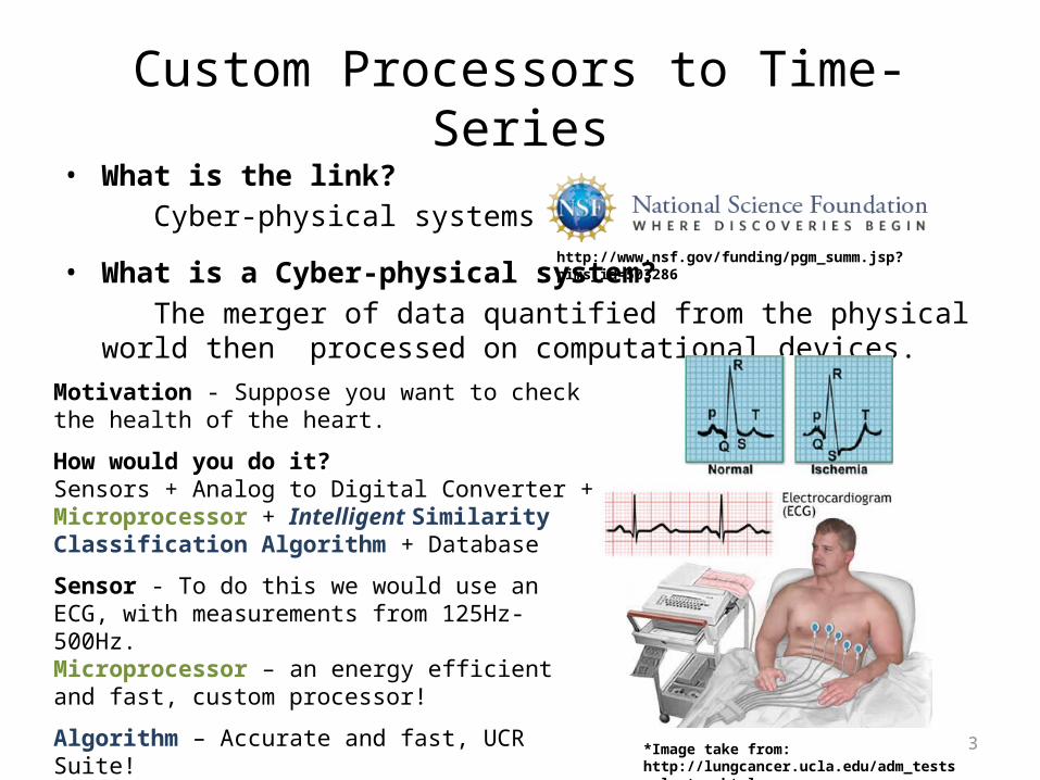
Custom Processors to Time-Series• What is the link?

Cyber-physical systems

• What is a Cyber-physical system? The merger of data quantified from the physical world then

processed on computational devices.

*Image take from: http://lungcancer.ucla.edu/adm_tests_electro.html

Motivation - Suppose you want to check the health of the heart.

How would you do it?Sensors + Analog to Digital Converter + Microprocessor + Intelligent Similarity Classification Algorithm + Database

Sensor - To do this we would use an ECG, with measurements from 125Hz-500Hz.Microprocessor – an energy efficient and fast, custom processor!

Algorithm – Accurate and fast, UCR Suite!

*A hospital charges $34,000 for a daylong EEG session to collect 0.3 trillion datapoints.

http://www.nsf.gov/funding/pgm_summ.jsp?pims_id=503286

4

What is a Time-Series?

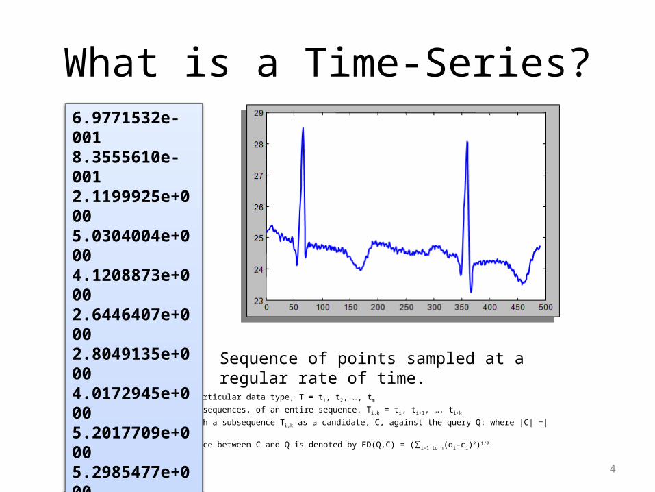
Formal Definition:• Ordered List of a particular data type, T = t1, t2, …, tm

• We consider only subsequences, of an entire sequence. T i,k = ti, ti+1, …, ti+k

• Objective is to match a subsequence Ti,k as a candidate, C, against the query Q; where |C| =|Q| = n

• The Euclidean Distance between C and Q is denoted by ED(Q,C) = (∑ i=1 to n(qi-ci)2)1/2

6.9771532e-001 8.3555610e-001 2.1199925e+0005.0304004e+000 4.1208873e+000 2.6446407e+000 2.8049135e+0004.0172945e+000 5.2017709e+000 5.2985477e+000 5.1660207e+000 4.4315405e+0004.0937909e+000 Sequence of points sampled at a regular rate of time.

5

What is Similarity?

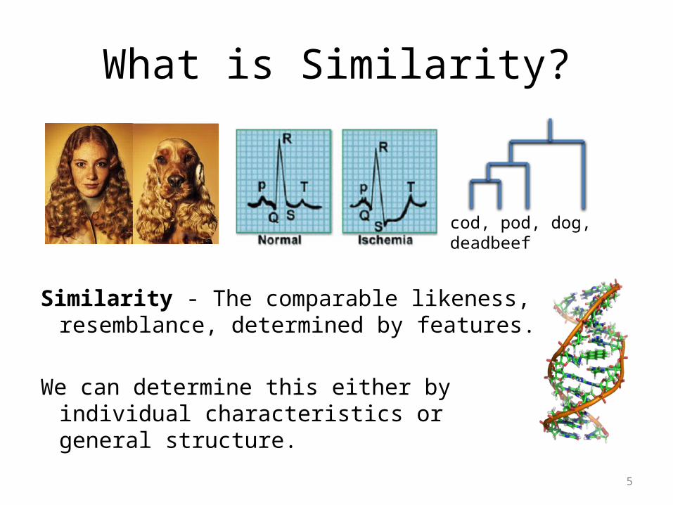
Similarity - The comparable likeness, resemblance, determined by features.

We can determine this either by individual characteristics or general structure.

cod, pod, dog, deadbeef

6

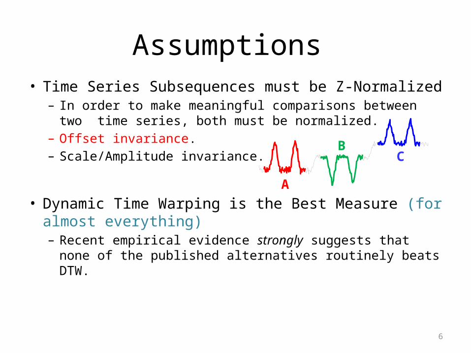
Assumptions • Time Series Subsequences must be Z-Normalized

– In order to make meaningful comparisons between two time series, both must be normalized.

– Offset invariance.– Scale/Amplitude invariance.

• Dynamic Time Warping is the Best Measure (for almost everything)– Recent empirical evidence strongly suggests that none of the

published alternatives routinely beats DTW.

A

BC

7

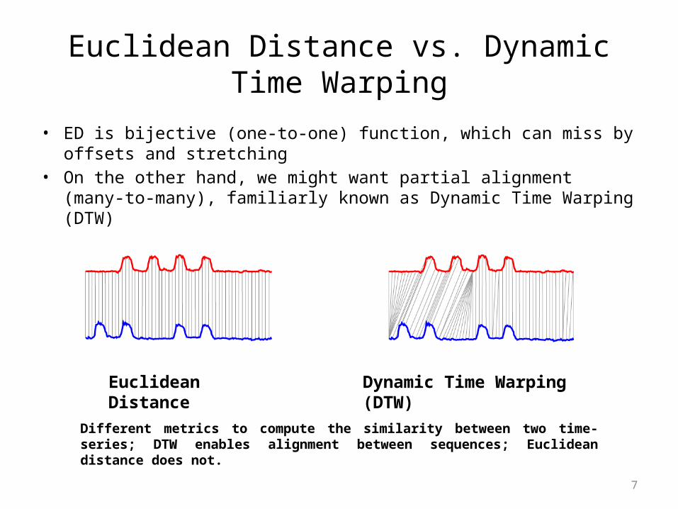
Euclidean Distance vs. Dynamic Time Warping

• ED is bijective (one-to-one) function, which can miss by offsets and stretching

• On the other hand, we might want partial alignment (many-to-many), familiarly known as Dynamic Time Warping (DTW)

Different metrics to compute the similarity between two time-series; DTW enables alignment between sequences; Euclidean distance does not.

Euclidean Distance Dynamic Time Warping (DTW)

8

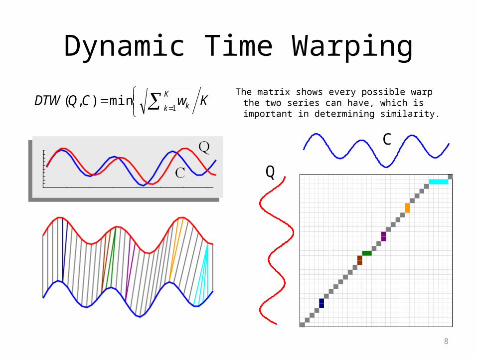
Dynamic Time WarpingThe matrix shows every possible warp the two

series can have, which is important in determining similarity.

C

Q

KwCQDTWK

k k1min),(

9

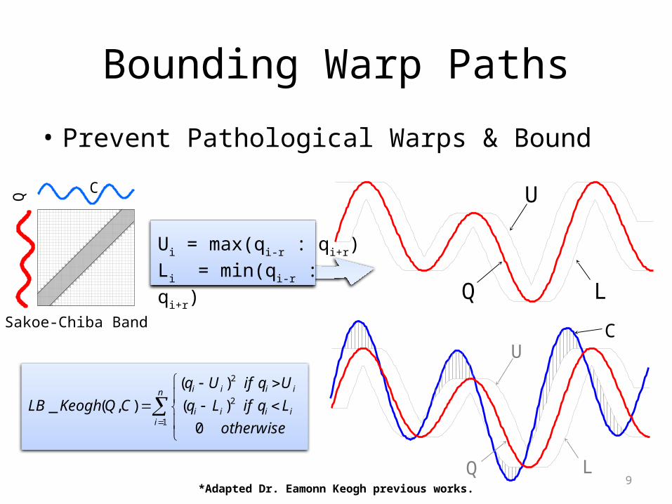
Bounding Warp Paths

• Prevent Pathological Warps & Bound

L

U

Q

C

Q

Sakoe-Chiba Band

Ui = max(qi-r : qi+r)Li = min(qi-r : qi+r)

CU

LQ

n

iiiii

iiii

otherwise

LqifLq

UqifUq

CQKeoghLB1

2

2

0

)(

)(

),(_

*Adapted Dr. Eamonn Keogh previous works.

10

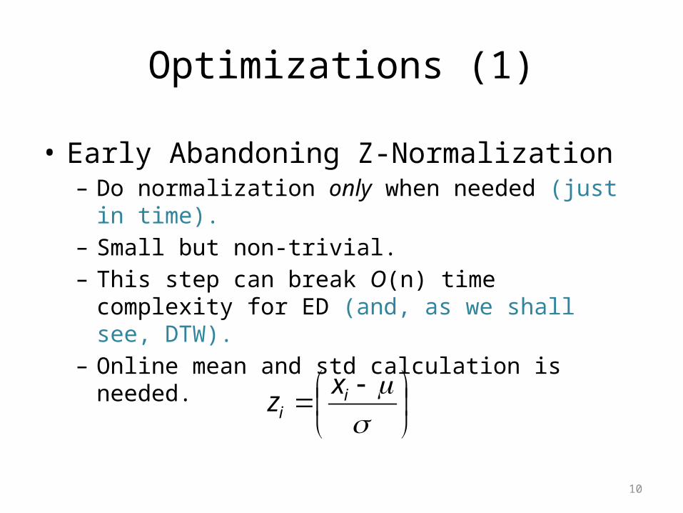
Optimizations (1)

• Early Abandoning Z-Normalization – Do normalization only when needed (just in time).– Small but non-trivial. – This step can break O(n) time complexity for ED (and, as

we shall see, DTW).– Online mean and std calculation is needed.

ii

xz

11

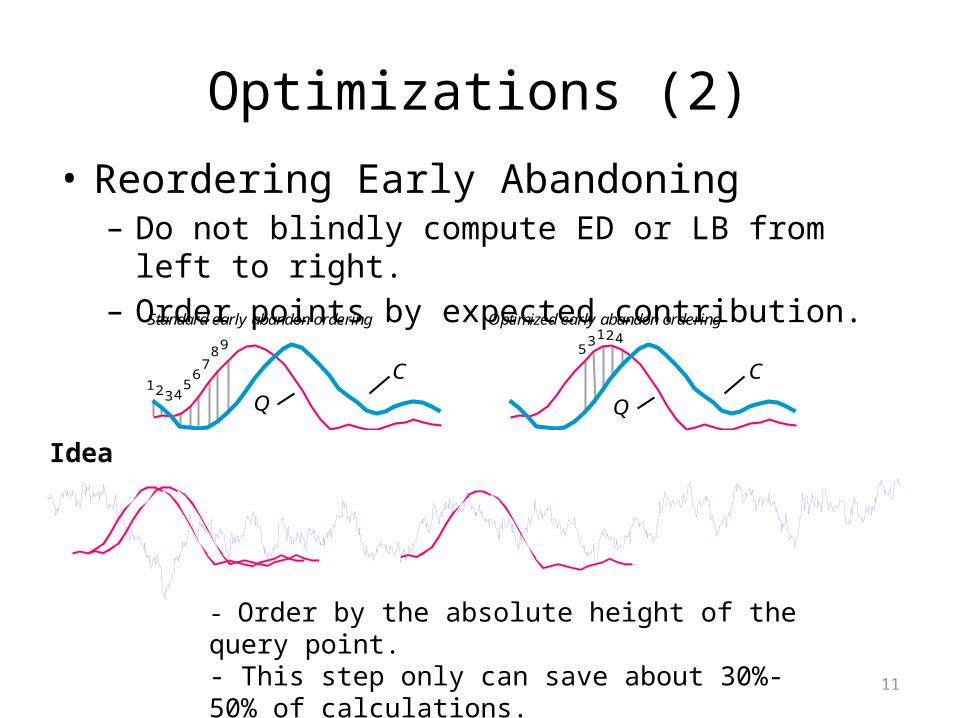
Optimizations (2)• Reordering Early Abandoning

– Do not blindly compute ED or LB from left to right.– Order points by expected contribution.

CC

Q Q1

32 4

65

7

983

51 42

Standard early abandon ordering Optimized early abandon ordering

- Order by the absolute height of the query point.- This step only can save about 30%-50% of calculations.

Idea

12

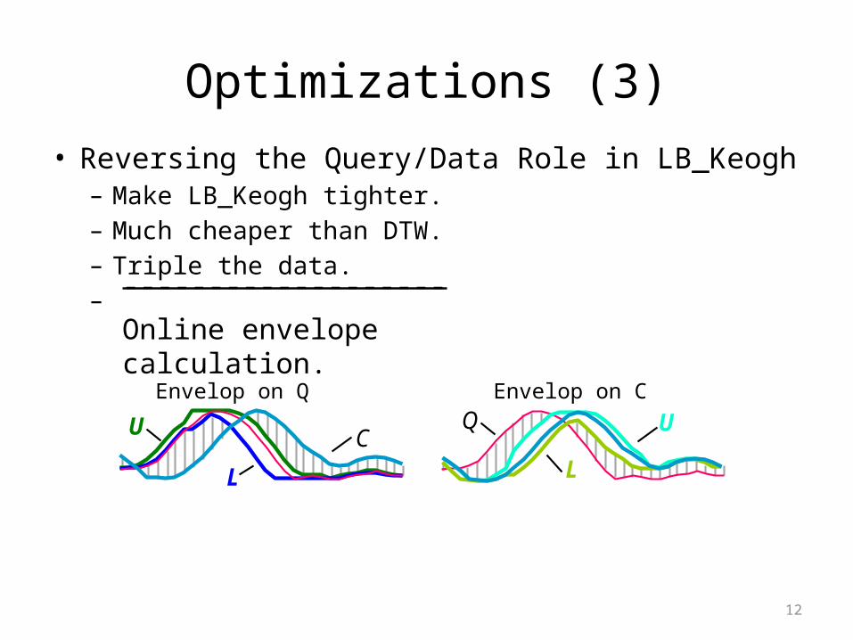
Optimizations (3)

• Reversing the Query/Data Role in LB_Keogh– Make LB_Keogh tighter.– Much cheaper than DTW.– Triple the data.–

CU

L

UQ

L

Envelop on Q Envelop on C

-------------------

Online envelope calculation.

13

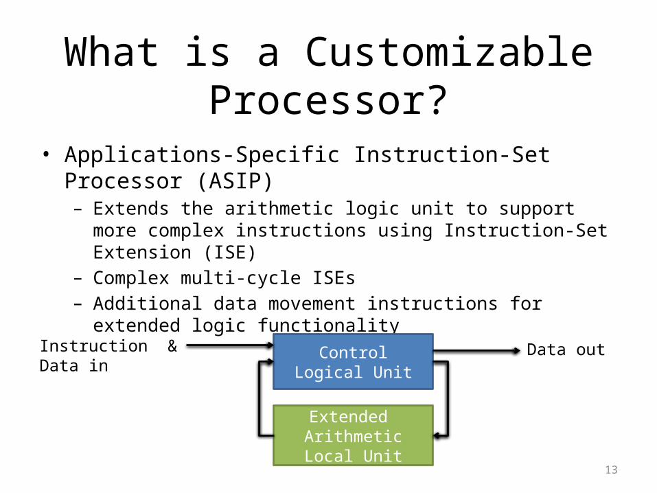
What is a Customizable Processor?

• Applications-Specific Instruction-Set Processor (ASIP)– Extends the arithmetic logic unit to support more complex instructions

using Instruction-Set Extension (ISE)– Complex multi-cycle ISEs– Additional data movement instructions for extended logic

functionality

Control Logical Unit

Extended Arithmetic Local Unit

Instruction & Data in Data out

14

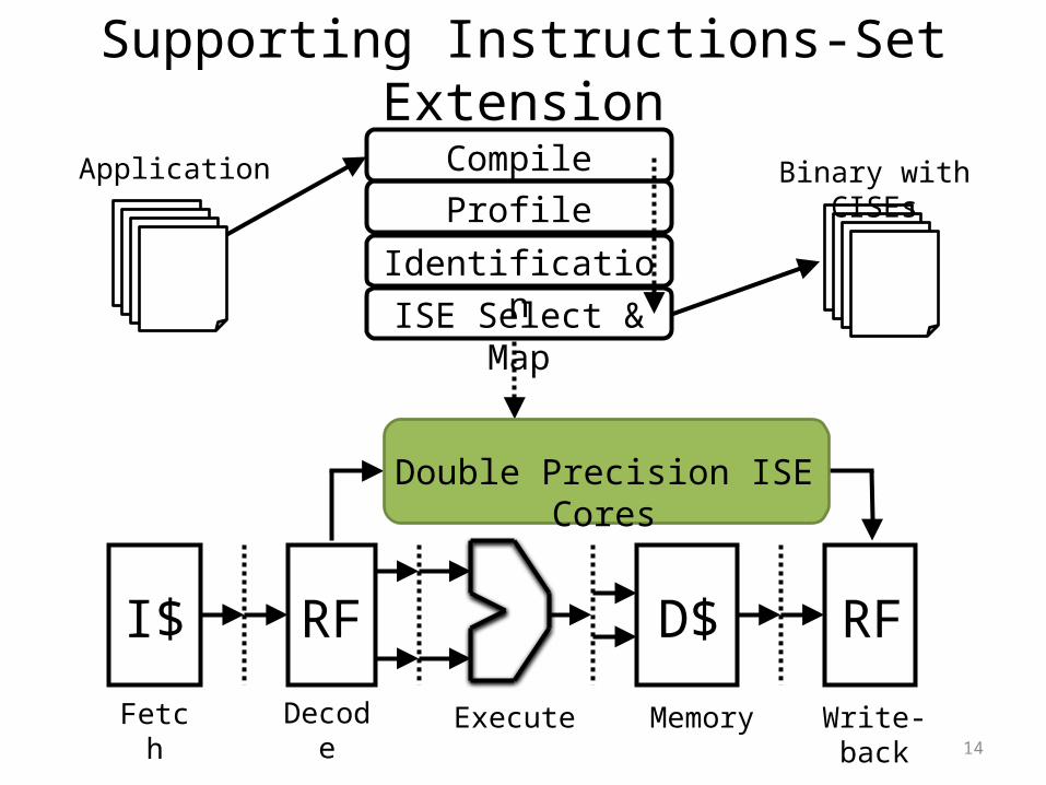
Supporting Instructions-Set Extension

I$ RF D$ RF

Fetch Decode Execute Memory Write-back

CompileProfile

Application Binary with CISEs

IdentificationISE Select & Map

Double Precision ISE Cores

15

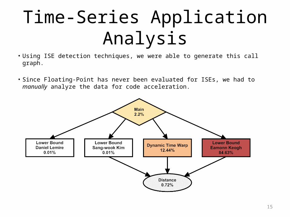
Time-Series Application Analysis• Using ISE detection techniques, we were able to generate this call graph.

• Since Floating-Point has never been evaluated for ISEs, we had to manually analyze the data for code acceleration.

16

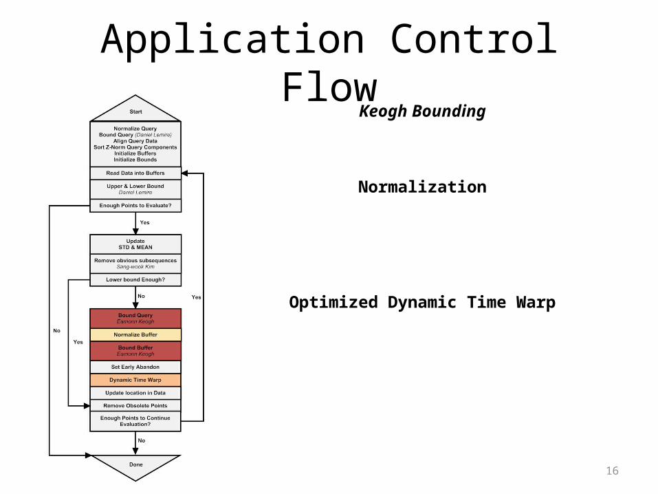
Application Control FlowKeogh Bounding

Normalization

Optimized Dynamic Time Warp

17

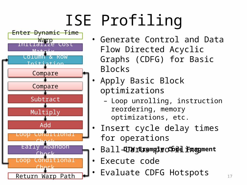
ISE Profiling

Column & Row Initiation

Initialize Cost Matrix

Loop Conditional Check

Early Abandon Check

Loop Conditional Check

Enter Dynamic Time Warp

Return Warp Path

Compare

Compare

Subtract

Multiply

Add

• Generate Control and Data Flow Directed Acyclic Graphs (CDFG) for Basic Blocks

• Apply Basic Block optimizations– Loop unrolling, instruction reordering,

memory optimizations, etc.

• Insert cycle delay times for operations• Ball-Larus profiling• Execute code• Evaluate CDFG Hotspots

DTW Example Code Fragment

18

>

Input 1 Input 2 Input 3 Input 4

Output 1

-

Example DFG

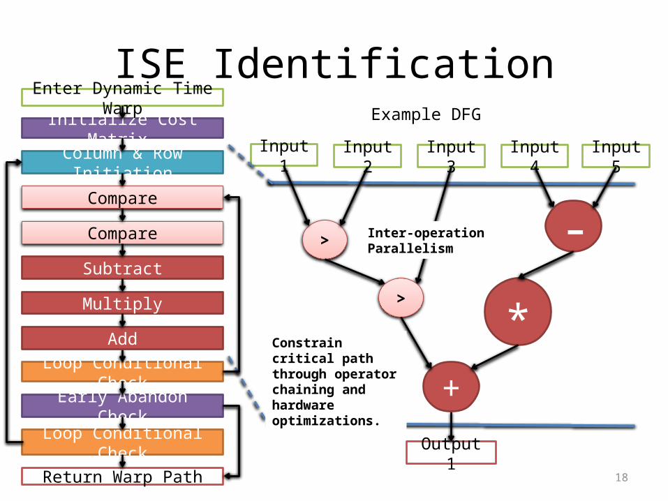
ISE Identification

Column & Row Initiation

Initialize Cost Matrix

Loop Conditional Check

Early Abandon Check

Loop Conditional Check

Enter Dynamic Time Warp

Return Warp Path

Compare

Compare

Subtract

Multiply

Add

Input 5

>

*+

Constrain critical path through operator chaining and hardware optimizations.

Inter-operation Parallelism

19

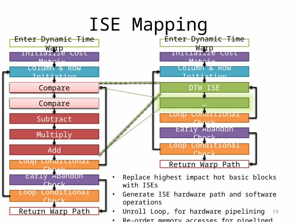
ISE Mapping

• Replace highest impact hot basic blocks with ISEs• Generate ISE hardware path and software operations• Unroll Loop, for hardware pipelining• Re-order memory accesses for pipelined ISEs

Column & Row Initiation

Initialize Cost Matrix

Loop Conditional Check

Early Abandon Check

Loop Conditional Check

Enter Dynamic Time Warp

Return Warp Path

Compare

Compare

Subtract

Multiply

Add

Column & Row Initiation

Initialize Cost Matrix

Loop Conditional Check

Early Abandon Check

Loop Conditional Check

Enter Dynamic Time Warp

Return Warp Path

DTW ISE

…

20

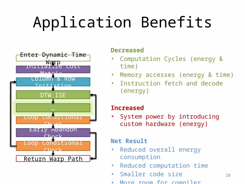
Application Benefits

Decreased• Computation Cycles (energy & time)• Memory accesses (energy & time)• Instruction fetch and decode (energy)

Increased • System power by introducing custom

hardware (energy)

Net Result• Reduced overall energy consumption• Reduced computation time• Smaller code size• More room for compiler optimizations

• E.G. Register coloring, code reordering, etc.

Column & Row Initiation

Initialize Cost Matrix

Loop Conditional Check

Early Abandon Check

Loop Conditional Check

Enter Dynamic Time Warp

Return Warp Path

DTW ISE

…

21

Iterative ISE Insertion

• Determine ISE cycle latencies– Software– FPU (Blocking)– ISEs (Pipelined)

• Adding all ISEs reduce the computation cycles by 3.43 x 1012 cycles

• 6.86x potential speedup

Baseline ISE-Norm ISE-NormISE-DTW

ISE-NormISE-DTW

ISE-Accum

ISE-NormISE-DTW

ISE-AccumISE-ED

0%

10%

20%

30%

40%

50%

60%

70%

80%

90%

100%

Normalization DTW ED

FP Accumulation Control Flow

ISE

Software

FPU Custom ISE Logic

Non-Pipelined (gcc -O0/O1)

Pipelined (gcc -O2/O3)

ISE-Norm ISE-DTW ISE-Accum ISE-SD

802 1851 433 889

613 1575 285 712

27 40 9 18

31 26 12 16

Latencies of ISEs in software (with and without pipelining), using floating-point operators, and specialized hardware ISE logic.

22

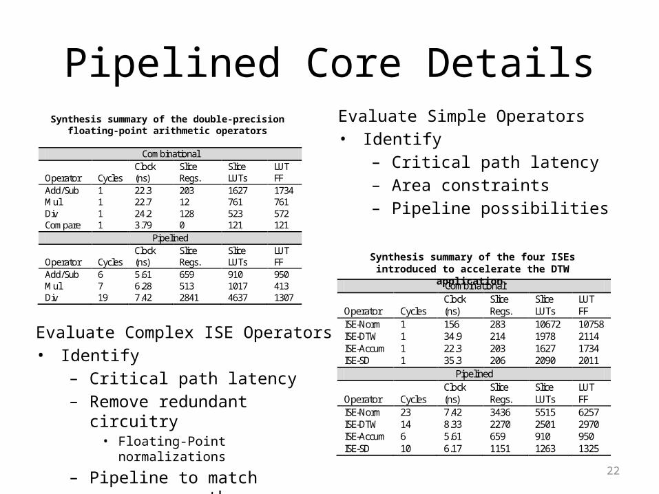
Pipelined Core Details

Combinational

Operator Cycles Clock (ns)

Slice Regs.

Slice LUTs

LUT FF

Add/Sub Mul Div Compare

1 1 1 1

22.3 22.7 24.2 3.79

203 12 128 0

1627 761 523 121

1734 761 572 121

Pipelined

Operator Cycles Clock (ns)

Slice Regs.

Slice LUTs

LUT FF

Add/Sub Mul Div

6 7 19

5.61 6.28 7.42

659 513 2841

910 1017 4637

950 413 1307

Combinational

Operator Cycles Clock (ns)

Slice Regs.

Slice LUTs

LUT FF

ISE-Norm ISE-DTW ISE-Accum ISE-SD

1 1 1 1

156 34.9 22.3 35.3

283 214 203 206

10672 1978 1627 2090

10758 2114 1734 2011

Pipelined

Operator Cycles Clock (ns)

Slice Regs.

Slice LUTs

LUT FF

ISE-Norm ISE-DTW ISE-Accum ISE-SD

23 14 6 10

7.42 8.33 5.61 6.17

3436 2270 659 1151

5515 2501 910 1263

6257 2970 950 1325

Synthesis summary of the double-precision floating-point arithmetic operators

Synthesis summary of the four ISEs introduced to accelerate the DTW application.

Evaluate Simple Operators• Identify

– Critical path latency– Area constraints– Pipeline possibilities

Evaluate Complex ISE Operators• Identify

– Critical path latency– Remove redundant circuitry

• Floating-Point normalizations

– Pipeline to match processor path

23

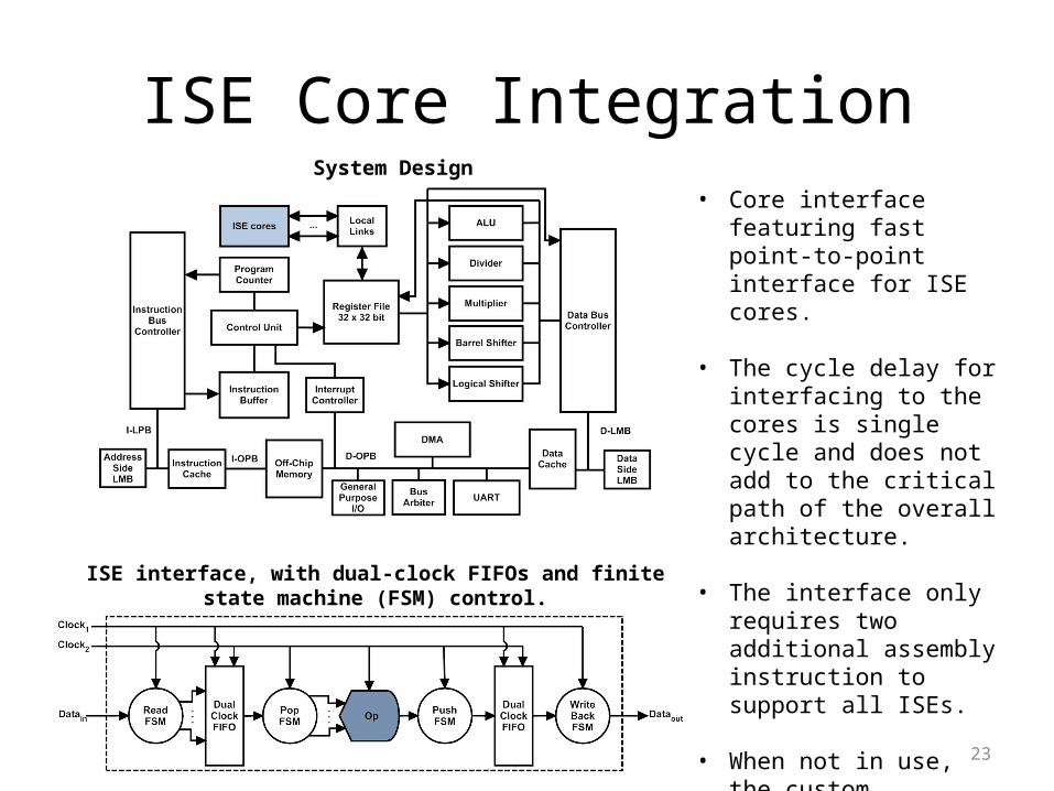
ISE Core Integration• Core interface featuring fast

point-to-point interface for ISE cores.

• The cycle delay for interfacing to the cores is single cycle and does not add to the critical path of the overall architecture.

• The interface only requires two additional assembly instruction to support all ISEs.

• When not in use, the custom Interface assigns low voltage to operator saving switching energy

ISE interface, with dual-clock FIFOs and finite state machine (FSM) control.

System Design

24

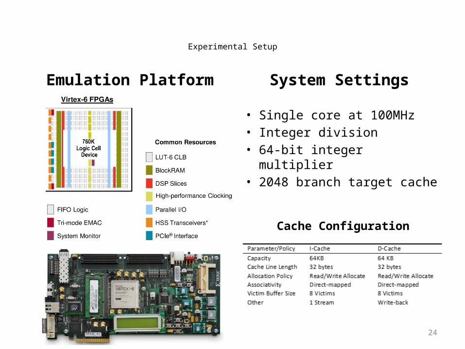
Experimental Setup

Emulation Platform System Settings

Virtex 6 ML605 FPGA

• Single core at 100MHz• Integer division• 64-bit integer multiplier• 2048 branch target cache

Cache Configuration

25

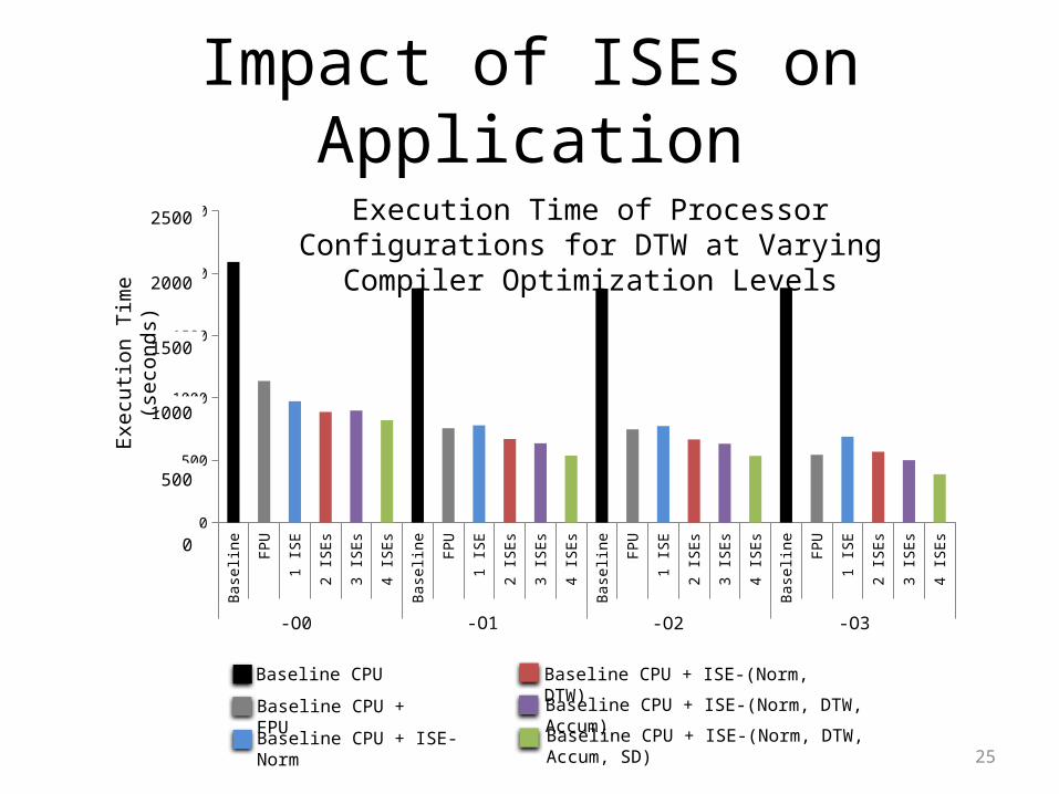
Impact of ISEs on Application

Base

line

FPU

1 IS

E

2 IS

Es

3 IS

Es

4 IS

Es

Base

line

FPU

1 IS

E

2 IS

Es

3 IS

Es

4 IS

Es

Base

line

FPU

1 IS

E

2 IS

Es

3 IS

Es

4 IS

Es

Base

line

FPU

1 IS

E

2 IS

Es

3 IS

Es

4 IS

Es

O0 O1 O2 O3

0

500

1000

1500

2000

2500

-O0 -O1 -O2 -O3

2500

2000

1500

1000

500

0

Exe

cutio

n T

ime

(sec

onds

)

Baseline CPU

Baseline CPU + FPU

Baseline CPU + ISE-Norm

Baseline CPU + ISE-(Norm, DTW)

Baseline CPU + ISE-(Norm, DTW, Accum)

Baseline CPU + ISE-(Norm, DTW, Accum, SD)

Execution Time of Processor Configurations for DTW at Varying Compiler Optimization Levels

26

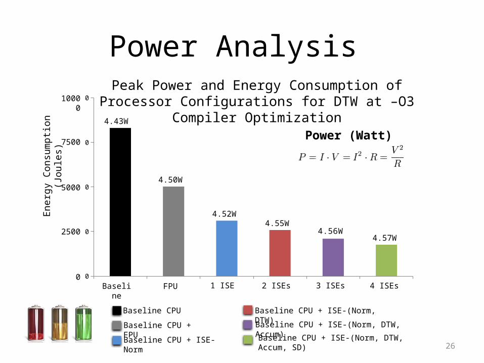
Power Analysis

Baseline CPU

Baseline CPU + FPU

Baseline CPU + ISE-Norm

Baseline CPU + ISE-(Norm, DTW)

Baseline CPU + ISE-(Norm, DTW, Accum)

Baseline CPU + ISE-(Norm, DTW, Accum, SD)

Baseline FPU 1 ISE 2 ISEs 3 ISEs 4 ISEs0

2500

5000

7500

10000

4.56W

10000

7500

5000

2500

0

Ene

rgy

Con

sum

ptio

n (J

oule

s)

Baseline FPU 1 ISE 2 ISEs 3 ISEs 4 ISEs

4.43W

4.50W

4.52W4.55W

4.57W

Peak Power and Energy Consumption of Processor Configurations for DTW at –O3 Compiler Optimization

Power (Watt)

27

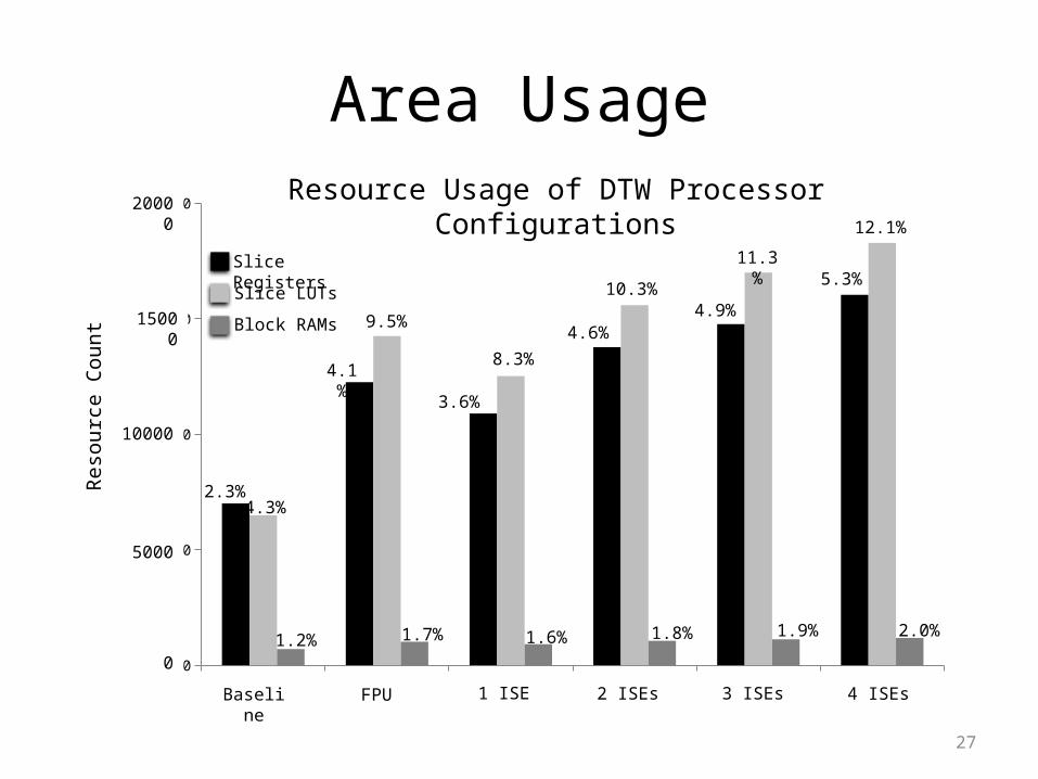
Area Usage

Baseline FPU 1 ISE 2 ISEs 3 ISEs 4 ISEs0

5000

10000

15000

20000

Baseline FPU 1 ISE 2 ISEs 3 ISEs 4 ISEs

20000

15000

5000

0

10000

Res

ourc

e C

ount

Slice Registers

Slice LUTs

Block RAMs

Resource Usage of DTW Processor Configurations

2.3%

1.2%

4.3%

4.1%

9.5%

1.7% 1.6% 1.8% 1.9% 2.0%

3.6%

8.3%

4.6%

10.3%4.9%

11.3%5.3%

12.1%

28

Results Summary

Speedup• Best software to best ISEs gives 4.86x speedup.•Compared to pipelined FPU, we are 1.42x

Area Of Baseline to ISE version• Memory increases 0.8%• LUTs increase 7.8%• Slices increase 3%

Energy• ISEs use 71% less energy of the pure software execution energy with twice area usage.•ISEs use 35% less energy than FPU

29

Conclusion & Future Work

• We have made a case for DTW in real world sensor networks.

• With the benefits of DTW ASIPs we can expect to get 4.87 times faster results with 78% less energy.

• Investigate root cause for loss of precision in fixed-point calculations.

• Determine best (numerical) strategy for embedded computation space.

• Extend ISE identification to consider floating-point calculations as a practical candidate for ASIPs.

• Build a lighter weight microcontroller to handle fixed and floating-point computations.

30

Questions