Integrating aerial and ship surveys of marine birds into a ...cels.uri.edu/docslink/McWilliams_pubs/Winiarski et al. 2014 (CONDOR... · Integrating aerial and ship surveys of marine

Volume 116, 2014, pp. 149–161DOI: 10.1650/CONDOR-13-085.1

RESEARCH ARTICLE

Integrating aerial and ship surveys of marine birds into a combineddensity surface model: A case study of wintering Common Loons

Kristopher J. Winiarski,1,3* M. Louise Burt,2 Eric Rexstad,2 David L. Miller,1 Carol L. Trocki,1 Peter W. C.Paton,1 and Scott R. McWilliams1

1 Department of Natural Resources Science, University of Rhode Island, Kingston, Rhode Island, USA2 Centre for Research into Ecological and Environmental Modelling, University of St Andrews, The Observatory, Buchanan Gardens, St

Andrews, Fife, United Kingdom3 Current address: Department of Environmental Conservation, University of Massachusetts, Amherst, Massachusetts, USA* Corresponding author: [email protected]

Received August 2, 2013; Accepted October 25, 2013; Published February 5, 2014

ABSTRACTBiologists now use a variety of survey platforms to assess the spatial distribution and abundance of marine birds, yetfew attempts have been made to integrate data from multiple survey platforms to improve model accuracy orprecision. We used density surface models (DSMs) to incorporate data from two survey platforms to predict thedistribution and abundance of a diving marine bird, the Common Loon (Gavia immer). We conducted strip transectsurveys from a multiengine, fixed-wing aircraft and line surveys from a 28 m ship during winter 2009–2010 in a 3,800km2 study area off the coast of Rhode Island, USA. We accounted for imperfect detection and availability bias due toCommon Loon diving behavior. We incorporated spatially explicit environmental covariates (water depth and latitude)to provide predictions of the spatial distribution and abundance of wintering Common Loons. The combined-platformDSM estimated the highest Common Loon densities (.20 individuals km�2) in nearshore waters ,35 m deep, with anaverage daily abundance of 5,538 (95% CI¼ 4,726–6,489) individuals in the study area. The combined-platform modeloffered substantial improvement in the precision of abundance estimates from the ship-platform model, and modestimprovement in the precision of the aerial-platform model. The combined model had relatively low predictive power,which previous research indicates is primarily a consequence of the dynamic marine environment. We show that theDSM approach presents a flexible framework for developing spatially explicit models of a marine bird from differentsurvey protocols.

Keywords: abundance estimation, Common Loon, density surface model, distance sampling, Gavia immer, spatialmodeling, spatially explicit abundance models

Integrando monitoreos en barco y aereos de aves marinas en un modelo combinado de densidad desuperficie: Un estudio de caso con Gavia immer durante el invierno

RESUMENLos biologos utilizan actualmente una variedad de plataformas de muestreo para evaluar la distribucion espacial yabundancia de aves marinas, sin embargo, existen pocos intentos para integrar datos de multiples plataformas demuestreo para mejorar la exactitud o precision del modelo. Utilizamos modelos de densidad de superficie (DSM) paraincorporar los datos de two plataformas de muestreo para predecir la distribucion y abundancia de un ave marinabuceadora, Gavia immer. Monitoreamos en transectos sectoriales con una aeronave de ala fija multimotor y muestreoslineales en un barco de 28 m, durante el invierno de 2009–2010, en un area de estudio de 3.800 km2, a las afueras de lacosta de Rhode Island. Consideramos la deteccion imperfecta, el sesgo de disponibilidad debido al comportamiento debuceo de Gavia immer, e incorporamos covariables ambientales espacialmente explıcitas (profundidad del agua ylatitud) para proveer predicciones de distribucion espacial y abundancia de invernacion de Gavia immer. La plataformacombinada de DSM estimo las densidades mas altas de Gavia immer (.20 individuos km�2) en las aguas cercanas a lacosta ,35 m de profundidad, con una abundancia promedio diaria de 5,538 (95 % IC¼4,726–6,489 ) individuos en el areade estudio. El modelo combinado de plataformas ofrecio una mejora sustancial en la precision de las estimaciones deabundancia que el modelo de plataforma desde el barco, y una modesta mejora en la precision del modelo de plataformaaerea. El modelo combinado produjo relativamente bajo poder predictivo; investigaciones anteriores indican que esto esconsecuencia, principalmente del ambiente marino dinamico. Demostramos que la propuesta DSM presenta un marcoflexible para desarrollar modelos espacialmente explıcitos de un ave marina con diferentes protocolos de monitoreo.

Palabras clave: estimaciones de abundancia, Gavia immer, modelo combinado de densidad de superficie,modelos espacialmente, modelos de abundancia espacialmente explıcitos

Q 2014 Cooper Ornithological Society. ISSN 0004-8038, electronic ISSN 1938-5129Direct all requests to reproduce journal content to the Central Ornithology Publication Office at [email protected]

INTRODUCTION

Ornithologists are interested in developing spatially

explicit estimates of avian abundance because they have

broad applications to avian ecology and conservation.

Robust distribution and abundance estimates of birds have

become more relevant with increasing conservation

concerns due to anthropogenic activities associated with

large-scale energy development. Currently, spatially ex-

plicit abundance estimates of marine birds are needed to

address the increasing interest in renewable energy

development in nearshore and offshore waters. This need

is especially relevant on the North American Atlantic

continental shelf, which has an estimated 4,000 GW of

potential wind energy (U.S. Department of Energy 2011).

The lack of information on the distribution and abundance

of marine birds, particularly at fine spatial scales, is due in

part to the paucity of systematic long-term marine bird

surveys in the region; however, spatially explicit abundance

estimates identify critical areas of high marine bird

densities and could be used to protect these areas from

development and reduce potential negative impacts (Fox et

al. 2006, Langston 2013).

Spatially explicit predictive abundance models have

recently been used to estimate the distribution and

abundance of marine birds (Clarke et al. 2003, Ainley et

al. 2009, Oppel et al. 2012, Winiarski et al. 2013). In

contrast to simply calculating density in areas directly

surveyed and multiplying that value by the total surveyarea to obtain an estimate of overall abundance, a spatially

explicit abundance model can incorporate relevant envi-

ronmental covariates (both biotic and abiotic) that may be

driving the distribution and abundance of a given marine

bird species. Such higher-resolution, spatially explicit

models allow more accurate predictions and identification

of areas important to the focal species or taxa (Clarke et al.

2003, Certain et al. 2007, Oppel et al. 2012).

For decades, systematic surveys from ships or aircraft

have been the primary platforms to determine the

distribution and abundance of marine birds (Ainley et al.

2012). Choice of platform often depends on target species

(i.e. some species cannot adequately be surveyed with ship

or aerial platforms), size of surveyed area, distance from

shore of surveyed area, budgetary constraints, safety

considerations, logistics, and specific research goals

(Camphuysen et al. 2004). Survey protocols with both

platforms have evolved to improve overall accuracy

(Tasker et al. 1984, Camphuysen et al. 2004, Ainley et al.

2012). Historically, strip transects were used with both

survey platforms, but line transects are now more common

because this protocol accounts for imperfect observer

detection probabilities (Buckland et al. 2001, Camphuysen

et al. 2004, Ronconi and Burger 2009). Over time, many

different governmental and nongovernmental organiza-

tions have collected data at different times using different

field methodologies. Recent interest in investigating

longer-term trends in abundance (e.g., to assess the impact

of climate change) means that combining these datasets is

essential to building a representative picture of distribu-

tion. Hence, combining marine bird survey data from

multiple platforms or protocols to increase overall

temporal or spatial coverage could improve overall model

performance and accuracy.

We integrated an aerial strip transect dataset with a

ship-based line transect dataset to develop a predictive

spatial model of a diving marine bird, the Common Loon

(Gavia immer), in southern New England, USA. We

selected Common Loons for this case study because they

are classified as a species of special concern in Massachu-

setts, New York, and Connecticut; threatened in New

Hampshire; and endangered in Vermont where they breed

(Evers et al. 2007, Kenow et al. 2009). Their sensitivity to

displacement from offshore wind energy development

(Petersen et al. 2006, Furness et al. 2013) makes the

Common Loon a marine bird of interest to biologists,

regulators, and developers in southern New England.

We first assessed data compatibility of Common Loon

abundance estimates between the 2 survey datasets and

then combined the datasets to model the distribution and

abundance of Common Loons wintering off the coast of

Rhode Island, USA, using a density surface model (DSM;

Hedley and Buckland 2004). DSM is a 2-stage approach:

(1) abundances are estimated over sections of each

transect (segments) using distance sampling methods for

line transect data; (2) estimated per-segment abundances

are then modeled as a function of environmental

covariates using generalized additive modeling (GAM;

e.g., Wood 2006). Due to the diving behavior of foraging

Common Loons, we also incorporated a correction for this

availability bias. Recently, the DSM approach has been

successfully used to predict the distribution and abun-

dance of sea ducks (Buckland et al. 2012), pinnipeds (Herr

et al. 2009), and mollusks (Katsanevakis 2007). Here we

present a DSM approach integrating ship- and aerial-based

survey platforms that used line and strip transect surveyprotocols, respectively.

METHODS

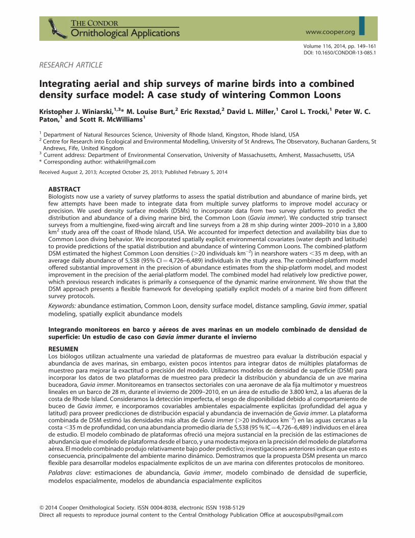
Study AreaWe conducted marine bird surveys off the coast of Rhode

Island, USA, in a 3,800 km2 study area in Rhode Island

Sound, Block Island Sound, and portions of the Inner

Continental Shelf (Figure 1). In early 2009, we initiated

ship-based line transect surveys to determine the distri-

bution and abundance of marine birds in the nearshore

and offshore waters as part of the Rhode Island Ocean

Special Area Management Plan (OSAMP). By midsummer

The Condor: Ornithological Applications 116:149–161, Q 2014 Cooper Ornithological Society

150 Density surface model of Common Loons K. J. Winiarski, M. L. Burt, E. Rexstad, et al.

2009, additional sites for offshore wind facilities were

proposed in the OSAMP area, so we initiated aerial-based

strip transect surveys to increase overall spatial survey

coverage while continuing the ship-based line transect

surveys.

Systematic Surveys

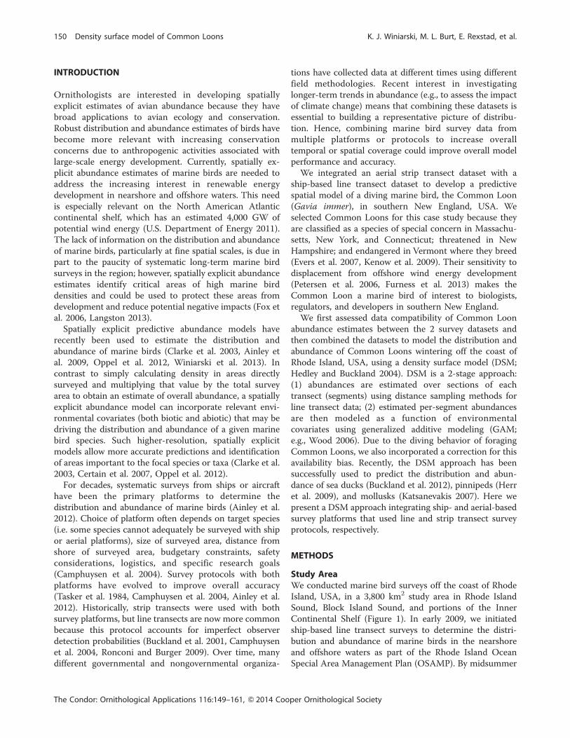
Ship-based surveys. We conducted ship-based surveys

on 8 grids randomly located across the study area (Figure

2) over 10 days between December 2, 2009, and February

13, 2010 (Supplemental Material Appendix A1). Each 69.8

km2 grid, 7.5 3 9.3 km, contained a 46 km sawtooth

transect that allowed observers to constantly stay on

survey, increasing overall effort (Figure 2). We were able to

survey 2 grids per day, given the speed constraints of the

ship. We surveyed 4 grids twice and the other 4 grids 3

times during the survey period (Supplemental Material

Appendix A1). The survey design tool in Distance 6.1 was

used to randomly place transect grids across the study area

(Thomas et al. 2010). Length of the transect grids was

determined by the transect distance we could sample

between dawn and 1400 hr including transportation time

to and from the sampling grids. Surveys were conducted

from the flying bridge (12 m ASL) of a 27.5 m long ship

traveling at 18.5 km hr�1 only when the Beaufort sea state

was ,4 and visibility was .1 km.

Using the ship-based line transect survey protocol

outlined in Camphuysen et al. (2004), we recorded the

distance and angle to each flock or nonflying Common

Loon that occurred within a ‘‘moving box’’ that extended

300 m in front of the bow of the ship and 300 m

perpendicular to the flying bridge. Sun glare determined

which side of the ship (port or starboard) was surveyed. All

surveys were conducted by one observer, and one

observer/recorder used unaided vision to initially detect

individual birds or flocks and then 10 3 42 power

FIGURE 1. Bathymetry of the Rhode Island Special Area Management Plan (OSAMP) study area. Darker shading indicates deeperwater. Block Island is located in the middle of the study area.


K. J. Winiarski, M. L. Burt, E. Rexstad, et al. Density surface model of Common Loons 151

http://dx.doi.org/10.1650/CONDOR-13-085.1.s1


binoculars to identify birds to species. Perpendicular

distance to each detection (an individual or flock) was

calculated from the estimated distance and bearing

(estimated using a large protractor mounted on the flying

bridge). We used a handheld global positioning system

(GPS)-enabled personal digital assistant (PDA; Trimble

Juno) using Cybertracker data collection software (Cape

Town, South Africa) to collect observation locations and a

handheld GPS (Garmin Marine GPS 76) to log the

coordinates of the ship every 15 s.

Aerial-based surveys. We conducted aerial surveys

along 24 fixed transects (Figure 2) on 9 days from

December 2, 2009, to February 22, 2010 (Supplemental

Material Appendix A1). We determined the location of the

24 transects using the survey design tool in Distance 6.1,

which placed a grid of transect lines at equally spaced

intervals across the study area at a random offset (Thomas

et al. 2010). In a 3.5 hr flight, we were able to survey 8

transect lines; thus, every third transect was visited on a

given flight, and all transect lines were sampled by

conducting ~3 flights per month. Each transect was

sampled 1–3 times during the survey period (Supplemen-

tal Material Appendix A1). Surveys were conducted from a

twin-engine Cessna 337 Skymaster flying at 185 km hr�1 at

152 m above the water surface. Following protocols used

by Perkins et al. (2005), 2 observers used unaided vision to

search 107-m-wide strip transects on either side of the

plane (0–44 m was not visible to observers). The

boundaries of the observation strip were denoted by

markings taped to the wing struts. Observers stopped

surveying when the sea state exceeded Beaufort state of 4,

or sometimes an observer on one side of the plane stopped

surveying when sun glare was intense. Detections were

recorded to the nearest second on a digital voice recorder

FIGURE 2. Common Loons (black circles) observed sitting on the water along aerial strip transects and ship line transects offsouthern Rhode Island during winter 2009–2010. Sawtooth lines represent 8 grids surveyed during ship-based surveys; the 24parallel vertical lines represent the aerial-based survey transects.





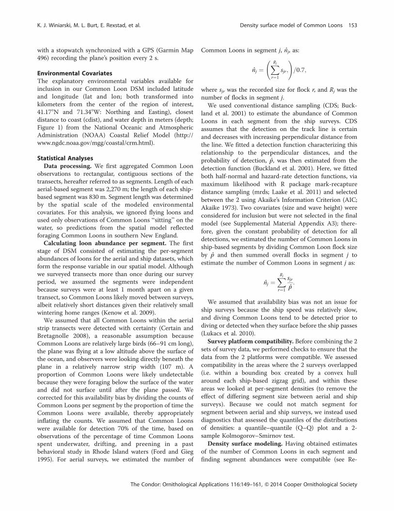
with a stopwatch synchronized with a GPS (Garmin Map

496) recording the plane’s position every 2 s.

Environmental CovariatesThe explanatory environmental variables available for

inclusion in our Common Loon DSM included latitude

and longitude (lat and lon; both transformed into

kilometers from the center of the region of interest,

41.178N and 71.348W: Northing and Easting), closest

distance to coast (cdist), and water depth in meters (depth;

Figure 1) from the National Oceanic and Atmospheric

Administration (NOAA) Coastal Relief Model (http://

www.ngdc.noaa.gov/mgg/coastal/crm.html).

Statistical AnalysesData processing. We first aggregated Common Loon

observations to rectangular, contiguous sections of the

transects, hereafter referred to as segments. Length of each

aerial-based segment was 2,270 m; the length of each ship-

based segment was 830 m. Segment length was determined

by the spatial scale of the modeled environmentalcovariates. For this analysis, we ignored flying loons and

used only observations of Common Loons ‘‘sitting’’ on the

water, so predictions from the spatial model reflected

foraging Common Loons in southern New England.

Calculating loon abundance per segment. The first

stage of DSM consisted of estimating the per-segment

abundances of loons for the aerial and ship datasets, which

form the response variable in our spatial model. Although

we surveyed transects more than once during our survey

period, we assumed the segments were independent

because surveys were at least 1 month apart on a given

transect, so Common Loons likely moved between surveys,

albeit relatively short distances given their relatively small

wintering home ranges (Kenow et al. 2009).

We assumed that all Common Loons within the aerial

strip transects were detected with certainty (Certain and

Bretagnolle 2008), a reasonable assumption because

Common Loons are relatively large birds (66–91 cm long),

the plane was flying at a low altitude above the surface of

the ocean, and observers were looking directly beneath the

plane in a relatively narrow strip width (107 m). A

proportion of Common Loons were likely undetectable

because they were foraging below the surface of the water

and did not surface until after the plane passed. We

corrected for this availability bias by dividing the counts of

Common Loons per segment by the proportion of time the

Common Loons were available, thereby appropriately

inflating the counts. We assumed that Common Loons

were available for detection 70% of the time, based on

observations of the percentage of time Common Loons

spent underwater, drifting, and preening in a past

behavioral study in Rhode Island waters (Ford and Gieg

1995). For aerial surveys, we estimated the number of

Common Loons in segment j, nj, as:

nj ¼XRj

r¼1sjr;

!=0:7;

where sjr was the recorded size for flock r, and Rj was the

number of flocks in segment j.

We used conventional distance sampling (CDS; Buck-

land et al. 2001) to estimate the abundance of Common

Loons in each segment from the ship surveys. CDS

assumes that the detection on the track line is certain

and decreases with increasing perpendicular distance from

the line. We fitted a detection function characterizing this

relationship to the perpendicular distances, and the

probability of detection, p, was then estimated from the

detection function (Buckland et al. 2001). Here, we fitted

both half-normal and hazard-rate detection functions, via

maximum likelihood with R package mark-recapture

distance sampling (mrds; Laake et al. 2011) and selected

between the 2 using Akaike’s Information Criterion (AIC;

Akaike 1973). Two covariates (size and wave height) were

considered for inclusion but were not selected in the final

model (see Supplemental Material Appendix A3); there-

fore, given the constant probability of detection for all

detections, we estimated the number of Common Loons in

ship-based segments by dividing Common Loon flock size

by p and then summed overall flocks in segment j to

estimate the number of Common Loons in segment j as:

nj ¼XRj

r¼1

sjr

p:

We assumed that availability bias was not an issue for

ship surveys because the ship speed was relatively slow,

and diving Common Loons tend to be detected prior to

diving or detected when they surface before the ship passes

(Lukacs et al. 2010).

Survey platform compatibility. Before combining the 2

sets of survey data, we performed checks to ensure that the

data from the 2 platforms were compatible. We assessed

compatibility in the areas where the 2 surveys overlapped

(i.e. within a bounding box created by a convex hull

around each ship-based zigzag grid), and within these

areas we looked at per-segment densities (to remove the

effect of differing segment size between aerial and ship

surveys). Because we could not match segment for

segment between aerial and ship surveys, we instead used

diagnostics that assessed the quantiles of the distributions

of densities: a quantile–quantile (Q–Q) plot and a 2-

sample Kolmogorov–Smirnov test.

Density surface modeling. Having obtained estimates

of the number of Common Loons in each segment and

finding segment abundances were compatible (see Re-




sults), we combined the Common Loon segment abun-

dance estimates from aerial and ship surveys. The per-

segment abundances, nj, were modeled as a function of the

spatially referenced covariates using a GAM of the

following form (assuming a log link function):

E nj� �¼ exp

�logðajÞ þ b0 þ bsurveyzsurvey þ

XKk¼1

fkðzkjÞ�;

Where b0 is an intercept; fk are smooth functions of the K

spatially referenced explanatory variables (see below), zkj;

the covariate zsurvey is a factor indicating the survey type

(ship or aerial) and has corresponding coefficient bsurvey.

The term log (aj) is an offset that corresponds to the area

of the segment, calculated as:

aj ¼ wjmjlj;

where wj is the width and lj is the length of segment j; and

the variable mj gives the number of sides of the platform

surveyed (only one side of the ship was surveyed at all

times).

We limited the maximum basis size for the smooth

terms to 7 for the univariate terms and 20 for the bivariate

terms. The maximum basis size controls the complexity of

the smooth terms; because the smooth terms were

penalized, only the maximum basis size needed to be set,

and the penalty reduced the complexity of the smooth

terms to an appropriate level while maintaining a good fit

(section 4.1.7 in Wood 2006; if necessary, the maximum

basis size can be increased). Survey platform was included

as a potential factor variable. We tested several response

distributions including negative binomial, quasi-Poisson,

Gamma, and Tweedie, and selected the appropriate

distribution by inspection of residual plots. We performed

model selection by building a model with all covariates

included and then removed terms if they were nonsignif-

icant (Supplemental Material Appendix A2). An additional

penalty was included for each smooth term, allowing their

degrees of freedom to be decreased below 1 (i.e. terms

were allowed to be completely removed from the model;

Wood 2006, section 4.1.6). We performed smoothness

selection by REstricted Maximum Likelihood (REML;

Wood 2011).

Once the model was selected, we calculated the

predicted abundance of Common Loons during winter

over the study area using spatially referenced data over 920

square grid cells. Each grid cell had a 2 km2 area that

served as the offset (aj, previous equation). Summing over

the predicted values yielded an estimate of abundance in

the study area. We calculated uncertainty in the abundance

estimates for each prediction grid cell and the overall

abundance using the variance propagation method of

Williams et al. (2011). This method incorporates uncer-

tainty from the estimation of the detection function

parameters (as well as from the GAM) by fitting a second

model (used only for variance calculations), which includes

an extra term (the derivative of p, with respect to the

detection function parameters) that accounts for the extra

variability incurred by the 2-step estimation procedure.

Uncertainty in the availability bias used to adjust counts

from the aerial survey could not be quantified and was not

included in variance estimates for abundance. Variance

propagation is not prone to the instabilities of simulation-

based variance estimation methods (e.g., moving block

bootstrap; Efron and Tibshirani 1994). To visualize the

uncertainty in the Common Loon abundance predictions

over the survey area, we calculated the coefficient of

variation for each prediction grid cell and plotted these as a

map of the region.

To ensure that the model was robust to several decisions

made as part of the modeling process, we analyzed the

sensitivity of our results. To check that the model was not

sensitive to varying the values of the availability correction,

we varied the availability correction value and looked at

the resulting Common Loon predicted abundance (Sup-

plemental Material Appendix A3). To investigate whether

correlations in Common Loon abundance estimates

between adjacent segments would affect the overall

Common Loon abundance estimate, we subsampled the

data to create 2 datasets in which every second segment

was selected, 3 datasets in which every third segment was

selected, and 4 in which every fourth segment was chosen.

From these resulting 9 datasets, Common Loon abundance

was then calculated using the methods outlined earlier

(Supplemental Material Appendix A3).

Using the models fitted to the subsets of the data,

predictions were made for those segments not included in

the model fitting process and compared with the

corresponding observed counts for each subset to indicate

the predictive power of the model. To quantify perfor-

mance, we fitted a linear model to the predicted counts for

the missing segments and used the observed (but

excluded) counts as an explanatory variable; the slope

coefficient of the resulting model can then be used forcomparison (a slope of 1 indicates perfect agreement

between excluded and observed counts and model

predictions). We used R version 2.15.1 (R Development

Core Team 2012) for all statistical analyses and models.

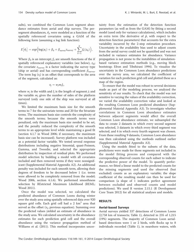
RESULTS

Aerial-based SurveysAerial surveys yielded 337 detections of Common Loons

(2,758 km of transects; Table 1), detected in 235 of 1,215

(19%) segments. The majority of Common Loon aerial-

based detections were 1 or 2 birds, with flocks up to 8

individuals recorded (Table 1), in nearshore waters, with






highest detections in waters southwest of Block Island

(Figure 2).

Ship-based Surveys

Ship surveys yielded 161 detections of Common Loons

(808 km of transects; Table 1) in 125 of 974 (13%)

segments. Similar to aerial surveys, the majority of

Common Loon ship-based detections were 1 or 2 birds,

with flocks of up to 4 individuals recorded (Table 1), in

nearshore waters, with highest detections in those waters

adjacent to southern Rhode Island’s coast and Block Island

(Figure 2).

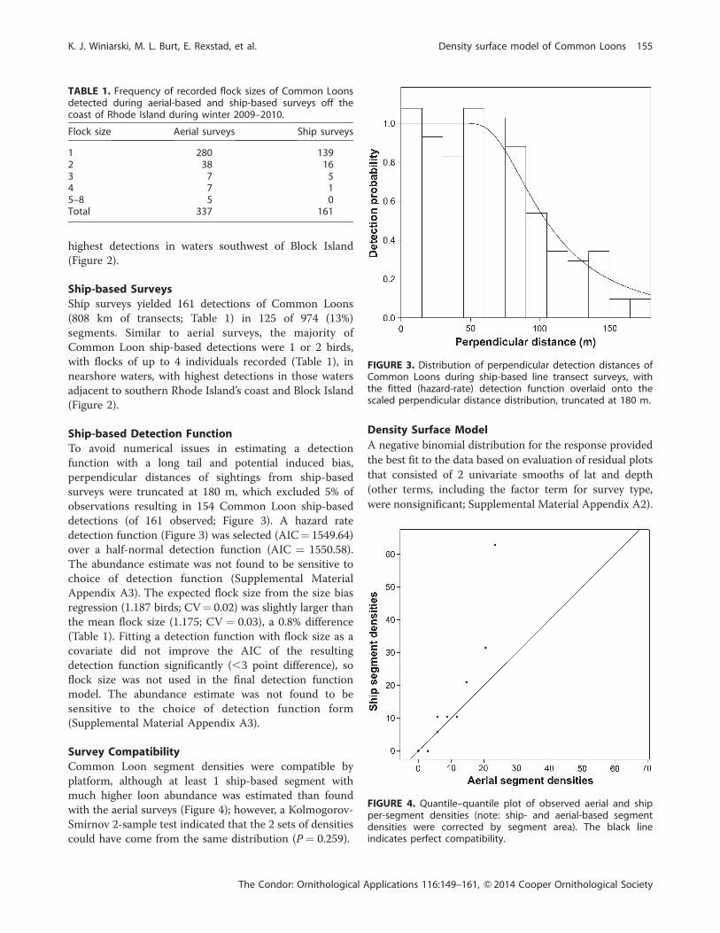
Ship-based Detection Function

To avoid numerical issues in estimating a detection

function with a long tail and potential induced bias,

perpendicular distances of sightings from ship-based

surveys were truncated at 180 m, which excluded 5% of

observations resulting in 154 Common Loon ship-based

detections (of 161 observed; Figure 3). A hazard rate

detection function (Figure 3) was selected (AIC¼ 1549.64)

over a half-normal detection function (AIC ¼ 1550.58).

The abundance estimate was not found to be sensitive to

choice of detection function (Supplemental Material

Appendix A3). The expected flock size from the size bias

regression (1.187 birds; CV¼ 0.02) was slightly larger than

the mean flock size (1.175; CV ¼ 0.03), a 0.8% difference

(Table 1). Fitting a detection function with flock size as a

covariate did not improve the AIC of the resulting

detection function significantly (,3 point difference), so

flock size was not used in the final detection function

model. The abundance estimate was not found to be

sensitive to the choice of detection function form


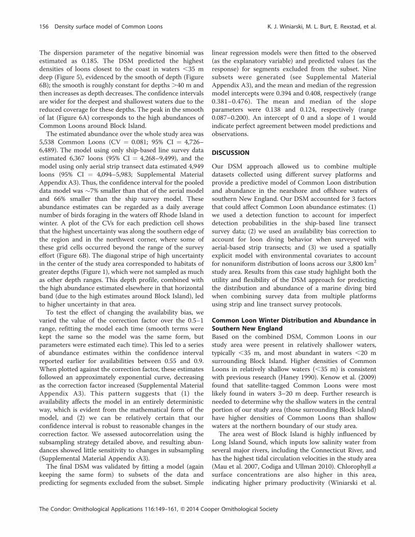
Survey Compatibility

Common Loon segment densities were compatible by

platform, although at least 1 ship-based segment with

much higher loon abundance was estimated than found

with the aerial surveys (Figure 4); however, a Kolmogorov-

Smirnov 2-sample test indicated that the 2 sets of densities

could have come from the same distribution (P ¼ 0.259).

Density Surface Model

A negative binomial distribution for the response provided

the best fit to the data based on evaluation of residual plots

that consisted of 2 univariate smooths of lat and depth

(other terms, including the factor term for survey type,

were nonsignificant; Supplemental Material Appendix A2).

TABLE 1. Frequency of recorded flock sizes of Common Loonsdetected during aerial-based and ship-based surveys off thecoast of Rhode Island during winter 2009–2010.

Flock size Aerial surveys Ship surveys

1 280 1392 38 163 7 54 7 15–8 5 0Total 337 161

FIGURE 3. Distribution of perpendicular detection distances ofCommon Loons during ship-based line transect surveys, withthe fitted (hazard-rate) detection function overlaid onto thescaled perpendicular distance distribution, truncated at 180 m.

FIGURE 4. Quantile–quantile plot of observed aerial and shipper-segment densities (note: ship- and aerial-based segmentdensities were corrected by segment area). The black lineindicates perfect compatibility.






The dispersion parameter of the negative binomial was

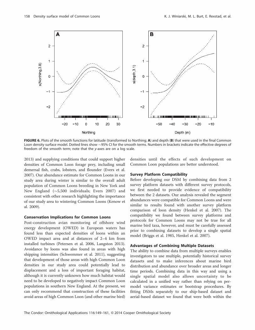
estimated as 0.185. The DSM predicted the highest

densities of loons closest to the coast in waters ,35 m

deep (Figure 5), evidenced by the smooth of depth (Figure

6B); the smooth is roughly constant for depths .40 m and

then increases as depth decreases. The confidence intervals

are wider for the deepest and shallowest waters due to the

reduced coverage for these depths. The peak in the smooth

of lat (Figure 6A) corresponds to the high abundances of

Common Loons around Block Island.

The estimated abundance over the whole study area was

5,538 Common Loons (CV ¼ 0.081; 95% CI ¼ 4,726–

6,489). The model using only ship-based line survey data

estimated 6,367 loons (95% CI ¼ 4,268–9,499), and the

model using only aerial strip transect data estimated 4,949

loons (95% CI ¼ 4,094–5,983; Supplemental Material

Appendix A3). Thus, the confidence interval for the pooled

data model was ~7% smaller than that of the aerial model

and 66% smaller than the ship survey model. These

abundance estimates can be regarded as a daily average

number of birds foraging in the waters off Rhode Island in

winter. A plot of the CVs for each prediction cell shows

that the highest uncertainty was along the southern edge of

the region and in the northwest corner, where some ofthese grid cells occurred beyond the range of the survey

effort (Figure 6B). The diagonal stripe of high uncertainty

in the center of the study area corresponded to habitats of

greater depths (Figure 1), which were not sampled as much

as other depth ranges. This depth profile, combined with

the high abundance estimated elsewhere in that horizontal

band (due to the high estimates around Block Island), led

to higher uncertainty in that area.

To test the effect of changing the availability bias, we

varied the value of the correction factor over the 0.5–1

range, refitting the model each time (smooth terms were

kept the same so the model was the same form, but

parameters were estimated each time). This led to a series

of abundance estimates within the confidence interval

reported earlier for availabilities between 0.55 and 0.9.

When plotted against the correction factor, these estimates

followed an approximately exponential curve, decreasing

as the correction factor increased (Supplemental Material

Appendix A3). This pattern suggests that (1) the

availability affects the model in an entirely deterministic

way, which is evident from the mathematical form of the

model, and (2) we can be relatively certain that our

confidence interval is robust to reasonable changes in the

correction factor. We assessed autocorrelation using the

subsampling strategy detailed above, and resulting abun-

dances showed little sensitivity to changes in subsampling


The final DSM was validated by fitting a model (again

keeping the same form) to subsets of the data and

predicting for segments excluded from the subset. Simple

linear regression models were then fitted to the observed

(as the explanatory variable) and predicted values (as the

response) for segments excluded from the subset. Nine

subsets were generated (see Supplemental Material

Appendix A3), and the mean and median of the regression

model intercepts were 0.394 and 0.408, respectively (range

0.381–0.476). The mean and median of the slope

parameters were 0.138 and 0.124, respectively (range

0.087–0.200). An intercept of 0 and a slope of 1 would

indicate perfect agreement between model predictions and

observations.

DISCUSSION

Our DSM approach allowed us to combine multiple

datasets collected using different survey platforms and

provide a predictive model of Common Loon distribution

and abundance in the nearshore and offshore waters of

southern New England. Our DSM accounted for 3 factorsthat could affect Common Loon abundance estimates: (1)

we used a detection function to account for imperfect

detection probabilities in the ship-based line transect

survey data; (2) we used an availability bias correction to

account for loon diving behavior when surveyed with

aerial-based strip transects; and (3) we used a spatially

explicit model with environmental covariates to account

for nonuniform distribution of loons across our 3,800 km2

study area. Results from this case study highlight both the

utility and flexibility of the DSM approach for predicting

the distribution and abundance of a marine diving bird

when combining survey data from multiple platforms

using strip and line transect survey protocols.

Common Loon Winter Distribution and Abundance inSouthern New EnglandBased on the combined DSM, Common Loons in our

study area were present in relatively shallower waters,

typically ,35 m, and most abundant in waters ,20 m

surrounding Block Island. Higher densities of Common

Loons in relatively shallow waters (,35 m) is consistent

with previous research (Haney 1990). Kenow et al. (2009)

found that satellite-tagged Common Loons were most

likely found in waters 3–20 m deep. Further research is

needed to determine why the shallow waters in the central

portion of our study area (those surrounding Block Island)

have higher densities of Common Loons than shallow

waters at the northern boundary of our study area.

The area west of Block Island is highly influenced by

Long Island Sound, which inputs low salinity water from

several major rivers, including the Connecticut River, and

has the highest tidal circulation velocities in the study area

(Mau et al. 2007, Codiga and Ullman 2010). Chlorophyll a

surface concentrations are also higher in this area,

indicating higher primary productivity (Winiarski et al.







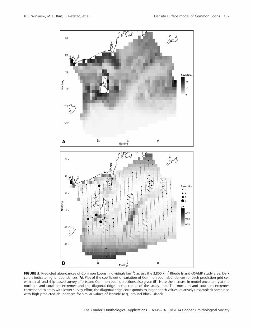
FIGURE 5. Predicted abundances of Common Loons (individuals km�2) across the 3,800 km2 Rhode Island OSAMP study area. Darkcolors indicate higher abundances (A). Plot of the coefficient of variation of Common Loon abundances for each prediction grid cellwith aerial- and ship-based survey efforts and Common Loon detections also given (B). Note the increase in model uncertainty at thenorthern and southern extremes and the diagonal ridge in the center of the study area. The northern and southern extremescorrespond to areas with lower survey effort; the diagonal ridge corresponds to larger depth values (relatively unsampled) combinedwith high predicted abundances for similar values of latitude (e.g., around Block Island).



2013) and supplying conditions that could support higher

densities of Common Loon forage prey, including small

demersal fish, crabs, lobsters, and flounder (Evers et al.

2007). Our abundance estimate for Common Loons in our

study area during winter is similar to the overall adult

population of Common Loons breeding in New York and

New England (~5,500 individuals; Evers 2007) and

consistent with other research highlighting the importance

of our study area to wintering Common Loons (Kenow et

al. 2009).

Conservation Implications for Common Loons

Post-construction avian monitoring of offshore wind

energy development (OWED) in European waters has

found less than expected densities of loons within an

OWED impact area and at distances of 2–4 km from

installed turbines (Petersen et al. 2006, Langston 2013).

Avoidance by loons was also found in areas with high

shipping intensities (Schwemmer et al. 2011), suggesting

that development of those areas with high Common Loon

densities in our study area could potentially lead to

displacement and a loss of important foraging habitat,

although it is currently unknown how much habitat would

need to be developed to negatively impact Common Loon

populations in southern New England. At the present, we

can only recommend that construction of these facilities

avoid areas of high Common Loon (and other marine bird)

densities until the effects of such development on

Common Loon populations are better understood.

Survey Platform Compatibility

Before developing our DSM by combining data from 2

survey platform datasets with different survey protocols,

we first needed to provide evidence of compatibility

between the 2 datasets. Our analysis revealed the segment

abundances were compatible for Common Loons and were

similar to results found with another survey platform

comparison of loon density (Henkel et al. 2007). The

compatibility we found between survey platforms and

protocols for Common Loons may not be true for all

marine bird taxa, however, and must be carefully assessed

prior to combining datasets to develop a single spatial

model (Briggs et al. 1985, Henkel et al. 2007).

Advantages of Combining Multiple DatasetsThe ability to combine data from multiple surveys enables

investigators to use multiple, potentially historical survey

datasets and to make inferences about marine bird

distribution and abundance over broader areas and longer

time periods. Combining data in this way and using a

single spatial model also allows uncertainty to be

calculated in a unified way rather than relying on per-

model variance estimates or bootstrap procedures. By

fitting DSMs separately to our ship-based dataset and

aerial-based dataset we found that were both within the

FIGURE 6. Plots of the smooth functions for latitude (transformed to Northing; A) and depth (B) that were used in the final CommonLoon density surface model. Dotted lines show ~95% CI for the smooth terms. Numbers in brackets indicate the effective degrees offreedom of the smooth term; note that the y-axes are on a log scale.



confidence interval of the combined model, but the

confidence interval for the combined-platform model

was ~7% smaller than the aerial-platform model and

66% smaller than the ship-platform model. Given that

ship-based surveys covered only ~15% of the our study

area, the improvement in the precision of the ship-based

model by integrating aerial surveys, which had much

broader coverage of our study area, was not unexpected.

Previous studies have shown that density estimates can

vary for some species between aerial and ship surveys

(Briggs et al. 1985), and the ability to identify individuals to

species can vary between survey platforms (Briggs et al.

1985), so care must be taken before combining datasets.

Investigators wishing to incorporate many surveys into a

single DSM should consider the compatibility checks

described in this study before attempting to fit a DSM.

Advantages of a Density Surface Modeling ApproachUsing a DSM has several advantages over other modeling

techniques. Compared to approaches developed by Royle

et al. (2004) and Fiske and Chandler (2011), the choice of

response distribution is much greater. Although we did not

model detection jointly with the spatial distribution, this

omission is not particularly problematic because transects

are long compared to their width and spacing, so variation

‘‘along’’ a transect is much more important than ‘‘across’’it. The 2-stage approach also is not an issue for variance

estimation because we can propagate uncertainty from the

detection function through to the spatial model using themethod of Williams et al. (2011).

A GAM spatial model allows simple extensions

(compared with other spatial modeling techniques) to

include a temporal component as well as random effects

and correlation structures, in addition to smooth terms to

improve our understanding of the distribution of CommonLoons off the coast of New England in both space and

time. GAMs also offer the advantage that their interpre-

tation follows from generalized linear model theory, so

interpretation and model checking procedures are well-

developed and relatively straightforward for nonexperts.

Improving Future Marine Bird Predictive ModelsOur DSM had relatively low predictive power according to

our cross-validation procedure, which unfortunately is

typical of marine bird predictive models (Oppel et al. 2012,

Winiarski et al. 2013). The highly dynamic marine

environment and the brief time window in which

systematic marine bird surveys are usually conducted

inevitably reduces the predictive power of such models.

For example, these conditions may increase the number of

falsely zero-inflated counts (Oppel et al. 2012) or make it

difficult to accurately assess flock size for large flocks.

Although digital methods (Buckland et al. 2012) improve

some elements of data collection (specifically, detection is

certain in the recorded strip), they do not change the

dynamic nature of the marine environment, so it is unclear

how well these digital methods will improve model fit and

predictive power.

Our DSM seemed relatively insensitive to the availability

bias correction factor, but it would be useful to improve

these estimates with further studies. Availability bias is

likely not constant and depends on environmental factors

(e.g., water depth or day length) or important periods in

marine bird annual life history, such as molt, which may

require increased forage consumption and hence more

time underwater unavailable to the observer. Improved

availability bias measures and variability of this metric

could be included in future spatial marine bird predictive

models (Buckland et al. 2012). Recent work by Borchers et

al. (2013) describes possible adaptations of current survey

methodology that could be used for this purpose to

validate our results, although they may potentially be

difficult to implement for marine birds. Chandler et al.

(2011) provides an approach that could provide stronger

estimates of availability bias in the future with repeated

surveys and these types of spatial models. Also, marine

bird distribution and abundance is likely strongly tied to

the distribution, abundance, and availability of prey items.

Without spatial data available for many lower tropic level

organisms, we can only use environmental covariates to

serve as proxies for prey distribution and density.

Improved input data will lead to predictive models with

higher confidence in their estimates, which is important

when using these models to guide future industrial marine

development to reduce risk to marine birds.

ACKNOWLEDGMENTS

We wish to thank the following people for their assistancewith various aspects of the project: observers Brian Harris,Alex Patterson, and John Veale for help collecting survey data;George Breen for piloting the Cessna Skymaster; Frances Fleetand their many captains for navigating the survey ship; ChrisDamon and Aimee Mandeville (URI EDC) for assistance withGIS analysis. J. F. Piatt, S. Oppel, and an anonymous reviewerprovided helpful comments that greatly improved thismanuscript. This research was supported by grant supportfrom the State of Rhode Island for the Ocean Special AreaManagement Plan.

LITERATURE CITED

Ainley, D. G., K. D. Dugger, R. G. Ford, S. D. Pierce, D. C. Reese, R.D. Brodeur, C. T. Tynan, and J. A. Barth (2009). Association ofpredators and prey at frontal features in the CaliforniaCurrent: Competition, facilitation, and co-occurrence. MarineEcology Progress Series 389:271–294.

Ainley, D. G., C. A. Ribic, and E. J. Woehler (2012). Adding theocean to the study of seabirds: A brief history of at-sea



seabird research. Marine Ecology Progress Series 451:231–243.

Akaike, H. (1973). Information theory and an extension of themaximum likelihood principle. In Second InternationalSymposium on Information Theory (B.N. Petrov and F.Csa’aki, Editors.). Akademiai Kiado, Budapest, Hungary. pp.267–281.

Borchers, D. L., W. Zucchini, M. P. Heide-Jørgensen, and A.Canadas (2013). Using hidden Markov models to deal withavailability bias on line transect surveys. Biometrics 69:703–713.

Briggs, K. T., W. B. Tyler, and D. B. Lewis (1985). Comparison ofship and aerial surveys of birds at sea. Journal of WildlifeManagement 49:405–411.

Buckland, S. T., D. R. Anderson, K. P. Burnham, J. L. Laake, D. L.Borchers, and L. Thomas (2001). Introduction to DistanceSampling: Estimating Abundance of Biological Populations.Oxford University Press, London, UK.

Buckland, S. T., M. L. Burt, E. A. Rexstad, M. Mellor, A. E. Williams,and R. Woodward (2012). Aerial surveys of seabirds: Theadvent of digital methods. Journal of Applied Ecology 49:960–967.

Camphuysen, C. J., A. D. Fox, M. Leopold, and I. K. Petersen(2004). Towards standardized seabirds at sea census tech-niques in connection with environmental impact assess-ments for offshore wind farms. U.K. COWRIE 1 Report. RoyalNetherlands Institute for Sea Research, Texel, Netherlands.

Certain, G., E. Bellier, B. Planque, and V. Bretagnolle (2007).Characterising the temporal variability of the spatial distri-bution of animals: An application to seabirds at sea.Ecography 30:695–708.

Certain, G., and V. Bretagnolle (2008). Monitoring seabirdspopulation in marine ecosystem: The use of strip transectaerial surveys. Remote Sensing of Environment 112:3314–3322.

Chandler, R. B., J. A. Royle, and D. I. King (2011). Inference aboutdensity and temporary emigration in unmarked populations.Ecology 92:1429–1435.

Clarke, E. D., L. B. Spear, M. L. Mccracken, F. F. C. Marques, D. L.Borchers, S. T. Buckland, and D. G. Ainley (2003). Validatingthe use of generalized additive models and at-sea surveys toestimate size and temporal trends of seabird populations.Journal of Applied Ecology 40:278–292.

Codiga, D. L., and D. S. Ullman (2010). Characterizing the physicaloceanography of coastal waters off Rhode Island, Part 1:Literature review, available observations, and a representa-tive model simulation. Rhode Island Ocean Special AreaManagement Plan, Coastal Resources Center, Narragansett,RI, USA.

Efron, B., and R. J. Tibshirani (1994). An Introduction to theBootstrap. Chapman and Hall, New York, NY, USA.

Evers, D. C. (2007). Status assessment and conservation plan forthe Common Loon (Gavia immer) in North America. BRIReport 2007-20. U.S. Fish and Wildlife Service, Hadley, MA,USA.

Fiske, I., and R. Chandler (2011). Unmarked: An R package forfitting hierarchical models of wildlife occurrence andabundance. Journal of Statistical Software 43:1–23.

Ford, T. B., and J. A. Gieg (1995). Winter behavior of the CommonLoon. Journal of Field Ornithology 66:22–29.

Fox, A. D., M. Desholm, J. Kahlert, T. K. Christensen, and I. K.Petersen (2006). Information needs to support environmentalimpact assessment of the effects of European marineoffshore wind farms on birds. Ibis 148:129–144.

Furness, R. W., H. M. Wade, and E. A. Masden (2013). Assessingvulnerability of marine bird populations to offshore windfarms. Journal of Environmental Management 119:56–66.

Haney, J. C. 1990. Winter habitat of Common Loons on thecontinental shelf of the southeastern United States. WilsonBulletin 102:253–263.

Hedley, S. L., and S. T. Buckland (2004). Spatial models for linetransect sampling. Journal of Agricultural, Biological andEnvironmental Statistics 9:181–199.

Henkel, L. A., R. G. Ford, W. B. Tyler, and J. N. Davis (2007).Comparison of aerial and boat-based survey methods forMarbled Murrelets Brachyramphus marmoratus and othermarine birds. Marine Ornithology 35:145–151.

Herr, H., M. Scheidat, K. Lehnert, and U. Siebert (2009). Seals atsea: Modeling seal distribution in the German bight based onaerial survey data. Marine Biology 156:811–820.

Katsanevakis, S. (2007). Density surface modeling with linetransect sampling as a tool for abundance estimation ofmarine benthic species: The Pinna nobilis example in amarine lake. Marine Biology 152:77–85.

Kenow, K. P., D. Adams, N. Schoch, D. C. Evers, W. Hanson, D.Yates, L. Savoy, T. H. Fox, A. Major, R. Kratt, and J. Ozard(2009). Migration patterns and wintering range of CommonLoons breeding in the Northeastern United States. Water-birds 32:234–247.

Laake, J. L., D. L. Borchers, L. Thomas, D. L. Miller, and J. Bishop(2011). mrds: Mark-Recapture Distance Sampling. http://cran.r-project.org/web/packages/mrds/index.html

Langston, R. H. W. (2013). Birds and wind projects across thepond: A UK perspective. Wildlife Society Bulletin 37:5–18.

Lukacs, P. M., M. L. Kissling, M. Reid, S. M. Gender, and S. B. Lewis(2010). Testing assumptions of distance sampling of a pelagicseabird. The Condor 112:455–459.

Mau, J. C., D. P. Wang , D. S. Ullman, and D. L. Codiga (2007).Comparison of observed (HF radar, ADCP) and modelbarotropic tidal currents in the New York Bight and BlockIsland Sound. Estuarine, Coastal and Shelf Science 72:129–137.

Oppel, S., A. Meirinho, I. Ramırez, B. Gardner, A. F. O’Connell, P. I.Miller, and M. Louzao (2012). Comparison of five modellingtechniques to predict the spatial distribution and abundanceof seabirds. Biological Conservation 156:94–104.

Perkins, S., G. Sadoti, T. Allison, E. Jedrey, and A. Jones (2005).Relative waterfowl abundance within Nantucket Sound,Massachusetts during the 2004–2005 winter season. Massa-chusetts Audubon Society Technical Report, Lincoln, MA,USA.

Petersen, I. K., T. K. Christensen, J. Kahlert, M. Desholm, and A. D.Fox (2006). Final results of bird studies at the offshore windfarms at Nysted and Horns Rev, Denmark. National ResearchInstitute Report, Ronde, Denmark.

R Development Core Team (2012). R: A language andenvironment for statistical computing. R Foundation forStatistical Computing, Vienna. www.R-project.org

Ronconi, R. A., and A. E. Burger (2009). Estimating seabirddensities from vessel transects: Distance sampling andimplications for strip transects. Aquatic Biology 4:297–309.



Royle, J. A., D. K. Dawson, and S. Bates (2004). Modelingabundance effects in distance sampling. Ecology 85:1591–1597.

Schwemmer P., B. Mendel, N. Sonntag, V. Dierschke, and S.Garthe (2011). Effects of ship traffic on seabirds in offshorewaters: Implications for marine conservation and spatialplanning. Ecological Applications 21:1851–1860.

Tasker, M. L., P. Hope-Jones, T. Dixon, and B. F. Blake (1984).Counting seabirds at sea from ships: A review of methodsemployed and a suggestion for a standardized approach. TheAuk 101:567–577.

Thomas, L., S. T. Buckland, E. A. Rexstad, J. L. Laake, S. Strindberg,S. L. Hedley, J. R. B. Bishop, T. A. Marques, and K. P. Burnham(2010). Distance software: Design and analysis of distancesampling surveys for estimating population size. Journal ofApplied Ecology 47:5–14.

U.S. Department of Energy (2011). Offshore energy workshop. Ajoint workshop by the Energy Department’s office of Energy

Efficiency and Renewable Energy and the Department of theInterior’s Bureau of Ocean Energy Management. Washington,DC, USA.

Williams, R., S. L. Hedley, T. A. Branch, M. V. Bravington, A. N.Zerbini, and K. P. Findlay (2011). Chilean blue whales as acase study to illustrate methods to estimate abundance andevaluate conservation status of rare species. ConservationBiology 25:526–535.

Winiarski, K. J., D. L. Miller, P. W. C. Paton, and S. R. McWilliams(2013). A spatially explicit model of wintering common loons:Conservation implications. Marine Ecology Progress Series492:273–278.

Wood, S. N. (2006). Generalized Additive Models: An Introduc-tion with R. Chapman & Hall/CRC, New York, NY, USA.

Wood, S. N. (2011). Fast stable restricted maximum likelihoodand marginal likelihood estimation of semiparametric gen-eralized linear models. Journal of the Royal Statistical Society:Series B, Statistical Methodology 73:3–36.



Documents

Integrating aerial and ship surveys of marine birds into a ...cels.uri.edu/docslink/McWilliams_pubs/Winiarski et al. 2014 (CONDOR... · Integrating aerial and ship surveys of marine