Is

Pa

b

a

ARRAA

KSSDGU

1

natpnotAct(e[[

ilpta

1d

Applied Soft Computing 11 (2011) 1263–1274

Contents lists available at ScienceDirect

Applied Soft Computing

journa l homepage: www.e lsev ier .com/ locate /asoc

ntegrating dominance properties with genetic algorithms for parallel machinecheduling problems with setup times

ei-Chann Changa,∗, Shih-Hsin Chenb

Department of Information Management, Yuan-Ze University, 135 Yuan Tung Road, Chung-Li 32026, Taiwan, ROCDepartment of Electronic Commerce Management, Nanhua University, 32, Chungkeng, Dalin Chiayi 62248, Taiwan, ROC

r t i c l e i n f o

rticle history:eceived 8 September 2007eceived in revised form 18 February 2010ccepted 14 March 2010vailable online 19 March 2010

a b s t r a c t

This paper deals with an unrelated parallel machine scheduling problem with the objective of minimizingthe makespan. There are machine-dependent and job sequence-dependent setup times and all jobs areavailable at time zero. This is a NP-hard problem and a set of dominance properties are developed includ-ing inter-machine (i.e., adjacent and non-adjacent interchange) and intra-machine switching properties

eywords:chedulingetup timesominance propertiesenetic algorithm

as necessary conditions of job sequencing orders in an optimal schedule. As a result, by applying thesedominance properties for a given sequence, a near-optimal solution can be derived. In addition, a newmeta-heuristic is introduced by integrating the dominance properties with genetic algorithm to furtherimprove the solution quality for larger problems. The performance of this meta-heuristic is evaluated byusing benchmark problems from the literature. The intensive experimental results show that GADP canfind all optimal solutions for the small problems and outperformed the solutions obtained by the existing

lems.

nrelated parallel machine heuristics for larger prob

. Introduction

In most scheduling problems, the setup times are eithereglected or assumed to be part of the processing times. Thisssumption is acceptable when the ratio of the setup time tohe processing time is small. However, in the make-to-orderroduction environment the role of the setup time cannot beeglected because of the frequent changeovers and large amountf setups. Negligence of setup time leads to unrealistic results,hat is, the resulting schedules are not informative any more.pplications for parallel machine scheduling with setup areommon in many industries including painting, plastic, tex-ile, glass, semiconductor, chemical, and paper manufacturinge.g., Guinet and Dussauchy [20]; Chang et al. [5,11] Francat al. [15]; Radhakrishnan and Ventura [36]; Kurz and Askin25]; Pinedo [34]; Randhawa and Kuo [29]; Zhang and Wu40]).

The unrelated parallel machines scheduling problem (PMSP)s the scheduling of n jobs available at time zero on m unre-

ated machines (Rm) to minimize the makespan, Cmax. If the jobs’rocessing times are dependent on the machine assigned andhere is no relationship among these machines, then the machinesre considered unrelated. In addition, machine-dependent and

∗ Corresponding author. Tel.: +886 936101320; fax: +886 34638884.E-mail address: iepchang@saturn.yzu.edu.tw (P.-C. Chang).

568-4946/$ – see front matter © 2010 Elsevier B.V. All rights reserved.oi:10.1016/j.asoc.2010.03.003

© 2010 Elsevier B.V. All rights reserved.

sequence-dependent setup times, i.e., Sijk, for job i sequenced beforej on machine k, are considered. The setup times are sequence-dependent as their amounts depend on job sequence. They are alsomachine-dependent because each machine has its own matrix ofsetup times and each machine is not exactly identical to each other.The problem will be referred to as Rm/Sijk/Cmax. The basic identicalPMSP Pm||Cmax is NP-hard even when m = 2 according to Garey andJohnson [16]. Since Rm/Sijk/Cmax is a generalization of the formerproblem, and then it is also NP-hard.

Recently, meta-heuristics are proposed to solve different kind ofmachine scheduling problems as in Chang et al. [6–10], Chou et al.[12], Hsieh et al. [21] and Connolly [13]. However, it is observedthat the convergence of genetic algorithm is slow. One way ofimproving the convergence in genetic algorithms is to includethe knowledge from problem domain. In this research, dominanceproperties are included in Meta-heuristics to further improve theconvergence. Dominance properties of the optimal schedule aredeveloped based on the switching of two adjacent jobs i and j. Thesedominance properties are in the mathematic form which providesnecessary conditions for any given schedule to be optimal. For agiven schedule, by applying these DP in advance, we can derivethe best sequence between any two jobs i and j. In addition, the

operation of DP is very efficient.

The dominance properties obtain efficient solutions before themeta-heuristics are carried out. Once the DP generates good initialsolutions efficiently, the meta-heuristics are able to converge faster.It is true that DP needs additional computational efforts, but helps

1 Soft C

Go

2

iAiwpws

iBtriBrtstDfpn

atmdasgr[tfGtToribsnbtd

laflptpicfahwl

264 P.-C. Chang, S.-H. Chen / Applied

A to converge faster so that meta-heuristics requires less numberf generations.

. Literature review

State-of-art reviews on parallel machines’ research can be foundn Graves [19], and more recently in Mokotoff [32]. In addition,llahverdi et al. [1] presented a survey on scheduling problems

nvolving setup time’s constraints. While the focus of our reviewill be limited to unrelated PMSP, it is important to note that manyapers addressed identical parallel machine scheduling with andithout setup consideration referring to recent researches by Dun-

tall and Wirth [14], Kurz and Askin [25], and Lin and Li [28].Allahverdi et al. [1] has provided a good review about schedul-

ng with setup time. Picard and Queyranne [33], Asano and Ohta [3],rucker et al. [4], have developed branch and bound algorithms forhis type of problems. Liu and Chang [29] proposed a Lagrangianelaxation-based approach. Martello et al. [39] proposed a mixednteger programming model and heuristic algorithms. Kim andobrowski [24] combined neural networks with some dispatchingules. Tan et al. [39] applied four different methods in solving theotal tardiness minimization problem of the single machine withequence-dependent setup times. Missbauer [31] investigated theopic about order release and sequence-dependent setup times.ue to the complexity of the problem, finding optimal solutions

or large problems is very time consuming and sometimes com-utationally infeasible. Developing heuristic algorithms to deriveear-optimal solutions becomes much more practical and useful.

Some authors have considered the use of meta-heuristicpproaches for unrelated PMSP. Kim et al. [22,23] developed heuris-ics for the problem including a Simulated Annealing (SA) to

inimize the total tardiness with machine-independent sequence-ependent setup times. Glass et al. [18] compared geneticlgorithms (GA), SA, and Tabu Search (TS) for Rm||Cmax withoutetup times. The authors concluded that the quality of solutionsenerated by GA was poor. However, a hybrid method that incorpo-ated GA was comparable to performances by SA and TS. Srivastava38] presented effective TS for the same problem without setupimes and reported that TS can provide good quality solutionsor practical size problems within a reasonable amount of time.hirardi and Potts [17] also addressed Rm||Cmax where the heuris-

ic they used was an application of the Recovering Beam Search.he authors reported that their algorithm produced good resultsn large instances (up to 50 machines and 1000 jobs). Someesearchers developed exact algorithms for unrelated PMSP includ-ng Liaw et al. [27] and Lancia [26] who developed branch andound algorithms to find optimal solutions for the problem withoutetup times. The objective functions are the total weighted tardi-ess and Cmax, respectively. Martello et al. [30] developed lowerounds for Rm||Cmax based on Lagrangian relaxation, which showedo be better than previous bounds. They utilized their results toevelop effective approximate algorithms.

The motivation for this paper comes from the scheduling prob-em in a real-world factory. There are many types of productsnd the production of various types of products on the shopoor requires different setup times in the changeovers. In theast, researchers have spent much effort in solving the setupime scheduling problems. This research will develop dominanceroperties including inter-machine (i.e., adjacent and non-adjacent

nterchange) and intra-machine switching properties as necessaryonditions of job sequencing orders in an optimal schedule. There-

ore, by applying these dominance properties for a given sequence,near-optimal solution can be derived. In addition, a new meta-euristic is introduced by integrating the dominance propertiesith genetic algorithm to further improve the solution quality for

arger problems.

omputing 11 (2011) 1263–1274

3. Problem definition

A mixed integer program (MIP) is formulated to find optimalsolutions for the unrelated parallel machine scheduling problemswith sequence-dependent times. Similar formulation was used byGuinet and Dussauchy [20].

Minimize Cmax (1)

subject to

n∑i=0

i /= j

m∑k=1

xi,j,k = 1 ∀j = 1, ..., n (2)

n∑i = 0j /= h

xi,h,k −n∑

i = 0j /= h

xh,j,k = 0 ∀h = 1, ..., n (3)

∀k = 1, ..., m

Cj ≥ Ci +m∑

k=1

xi,j,k(Si,j,k + pj,k) + M

(m∑

k=1

xi,j,k − 1

)(4)

∀i = 0, ..., n ∀j = 1, ..., n

n∑j=0

x0,j,k = 1 ∀k = 1, ..., m (5)

xi,j,k ∈{

0, 1} ∀i = 0, ..., n, ∀j = 0, ..., n, ∀k = 1, ..., m (6)

C0 = 0 (7)

Cj ≥ 0 ∀j = 1, ..., n (8)

where, Cj: Completion time of job j, pjk: processing time of job jon machine k, Sijk: sequence-dependent setup time to process jobj after job i on machine k, S0jk: setup time to process job j first onmachine k, xijk: 1 if job j is processed directly after job I on machinek and 0 otherwise, x0jk: 1 if job j is the first job to be processedon machine k and 0 otherwise, Sj0k: 1 if job j is the last job tobe processed on machine k and 0 otherwise, M: a large positivenumber.

The objective (1) is to minimize the makespan. Constraints (2)ensure that each job is scheduled only once and processed by onemachine. Constraints (3) make sure that each job must neither bepreceded nor succeeded by more than one job. Constraints (4) areused to calculate completion times and to ensure that no job canprecede and succeed the same job. Constraints (5) ensure that nomore than one job can be scheduled first at each machine. Notethat there is no need for another set of constraints to guaranteethat only one is scheduled last on each machine because this isguaranteed by constrains (5) in conjunction with (3). Constraints(6) specify that the decision variable x is binary over all domains.Constraints (7) state that the completion time for the dummy job0 is zero and constraints (8) ensure that completion times are non-negative. Optimal solutions for the problem then can be obtainedby solving the MIP software solver.

4. Derivations of dominance properties

We consider the problem of scheduling n jobs into unrelatedparallel machines and to derive the dominance properties (neces-sary conditions) of the optimal schedule. In this section, we usethe objective function (Z(�)) for the makespan of schedule �.

P.-C. Chang, S.-H. Chen / Applied Soft C

Fig. 1. A parallel machine schedule.

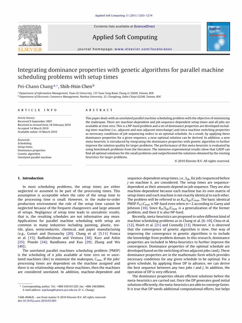
IcfaaoatAtjs

tmds

4

ina

Ls

(

Pa

Fig. 2. The interchange on the same machine (k1).

n order to derive the dominance properties for schedule �, weonsider interchanging two jobs on the same machine or on dif-erent machines to prove some intermediate results. Fig. 1 showsschematic diagram of a parallel machine schedule. [j]: The job ist position [j], P[j][k]: the processing time of the job at position [j]n machine [k], S[i][j][k]: the setup time of the job at position [j] isfter the job [i] on machine [k], AP[i][j][k]: the adjusted processingime of the job at position [j] is after the job [i] on machine [k]. Thus,P[i][j][k] is actually equal to P[j][k] plusS[i][j][k]. Ck1

: the completionime on k1, G1[k]: the job set before job [i] on machine k, G2[k]: theob set between job [i] and job [j + 1] on machine k, G2[k]: the jobet after job [i] on machine k.

There are two conditions in exchanging jobs and they includehe intra-machine (two jobs are on the same machine) and inter-

achine (The exchanging jobs come from different machines). Theominance properties of inter-machine and intra-machine are pre-ented at Sections 4.1 and 4.2, respectively.

.1. Inter-machine interchange

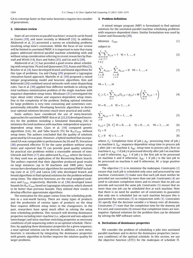
There are two cases to be considered within the inter-machinenterchange, and they are the adjacent exchange (see Fig. 2) andon-adjacent exchange (see Fig. 3). The following lemma is for thedjacent exchange.

emma 1a. When the following condition exists, the exchangedchedule is better than the original one:

AP[i−1][j][k] − AP[i−1][i][k]) + (AP[j][i][k] − AP[i][j][k])

+ (AP[i][j+1][k] − AP[j][j+1][k]) < 0

roof. Suppose we exchange job i and job j in schedule �x whichre adjacent to each other on the same machine. After exchanging

Fig. 3. Exchanging job i and job j on the same machine.

omputing 11 (2011) 1263–1274 1265

these two neighborhood jobs, schedule �x is changed to �y. FromFig. 2, the jobs in the set G1[k] and G′

1[k] remain the same, whoseobjective does not change. Thus, the completion time of G1[k] andG′

1[k] is shown as follows:

G1[k] =i−1∑a=1

AP[a−1][a][k] = G′1[k] �

Except for the G1[k] and G′1[k] are not changed, the completion

time of the job sets G′2[k], G′

3[k], G′2[k], and G′

3[k] are listed in thefollowing.

G2[k] = G1[k] + AP[i−1][i][k] + AP[i][j][k] + AP[j][j+1][k]

G3[k] = G2[k] +n∑

a=j+2

AP[a−1][a][k]

G′2[k] = G1[k] + AP[i−1][j][k] + AP[j][i][k] + AP[i][j+1][k]

G′3[k] = G′

2[k] +n∑

a=j+2

AP[a-1][a][k]

When it comes to calculate the difference before and after weexchange the job i and job j, we subtract �y with �x, whose differ-ence � is actually equal to G′

2[k] − G′3[k].

∴ � =∏

y−∏

x= G′

2[k]− G2[k]

= (AP[i−1][j][k] − AP[i−1][i][k]) + (AP[j][i][k] − AP[i][j][k]) + (AP[i][j+1][k] − AP[j][j+1][k])

As a result, if the difference � is less than zero, the job i and jobj should be exchanged.

In term of non-adjacent interchange, the procedure is similar.The dominance property of the non-adjacent interchange and thederivation are shown below.

Lemma 1b. When the following condition exists, the job i and job jare exchanged.

(AP[i−1][j][k] − AP[i−1][i][k]) + (AP[j][i+1][k] − AP[i][i+1][k])

+ (AP[j−1][i][k] − AP[j−1][j][k]) + (AP[i][j+1][k] − AP[j][j+1][k]) < 0

Proof. The objective of G1[k] and G′1[k], is the same, so it will be

eliminated after we subtract �y with �x. The equation of G1[k] andG′

1[k] is shown as follows:

G1[k] =i−1∑a=1

AP[a−1][a][k] = G′1[k] �

Similarly with the Lemma 1a, the completion time of the jobsets G2[k], G3[k], G′

2[k], and G′3[k] are changed. Thus, they are demon-

strated as follows.

G2[k] = G1[k] + AP[i−1][i][k] + AP[i][i+1][k] + AP[j−1][j][k] + AP[j][j+1][k]

n∑

G3[k] = G2[k] +

a=j+2

AP[a-1][a][k]

G′2[k] = G1[k] + AP[i−1][j][k] + AP[j][i+1][k] + AP[j−1][i][k] + AP[i][j+1][k]

1266 P.-C. Chang, S.-H. Chen / Applied Soft C

G

G

1][i][k

e

4

takeat

La

M , G3[

PMsItb

4

s

G

G

G

G

G

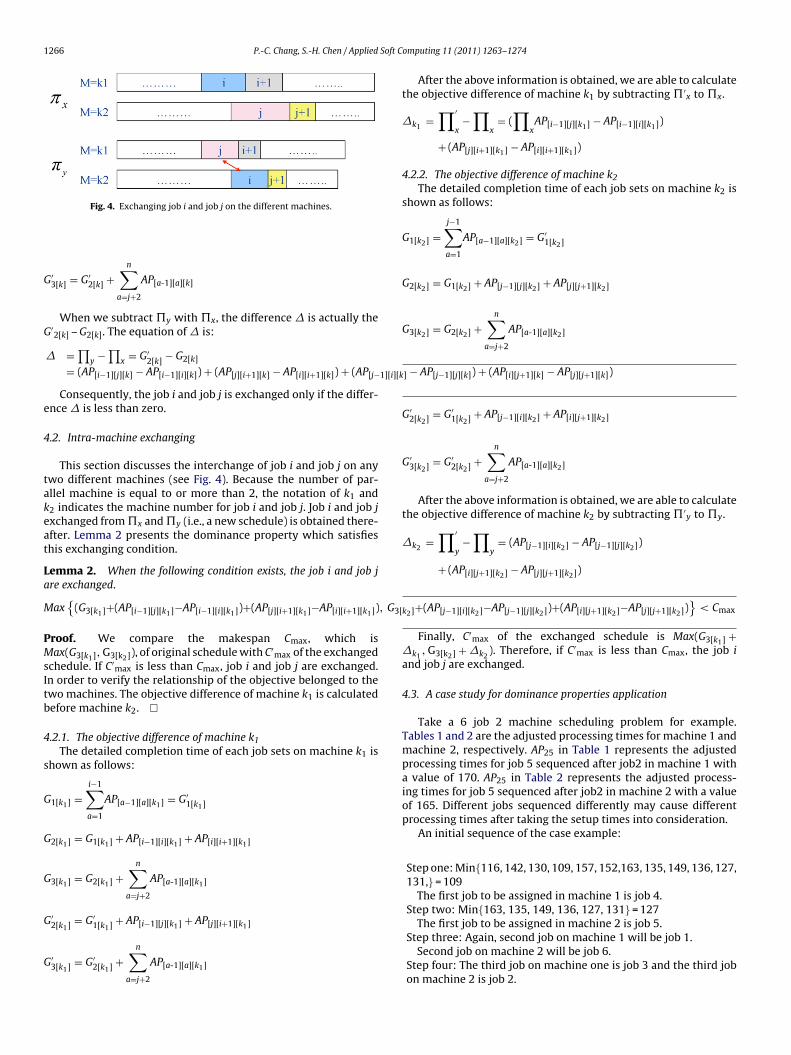
Fig. 4. Exchanging job i and job j on the different machines.

′3[k] = G′

2[k] +n∑

a=j+2

AP[a-1][a][k]

When we subtract �y with �x, the difference � is actually the′2[k] – G2[k]. The equation of � is:

� =∏y −∏x = G′2[k] − G2[k]

= (AP[i−1][j][k] − AP[i−1][i][k]) + (AP[j][i+1][k] − AP[i][i+1][k]) + (AP[j−

Consequently, the job i and job j is exchanged only if the differ-nce � is less than zero.

.2. Intra-machine exchanging

This section discusses the interchange of job i and job j on anywo different machines (see Fig. 4). Because the number of par-llel machine is equal to or more than 2, the notation of k1 and2 indicates the machine number for job i and job j. Job i and job jxchanged from �x and �y (i.e., a new schedule) is obtained there-fter. Lemma 2 presents the dominance property which satisfieshis exchanging condition.

emma 2. When the following condition exists, the job i and job jre exchanged.

ax{

(G3[k1]+(AP[i−1][j][k1]−AP[i−1][i][k1])+(AP[j][i+1][k1]−AP[i][i+1][k1])

roof. We compare the makespan Cmax, which isax(G3[k1], G3[k2]), of original schedule with C′

max of the exchangedchedule. If C′

max is less than Cmax, job i and job j are exchanged.n order to verify the relationship of the objective belonged to thewo machines. The objective difference of machine k1 is calculatedefore machine k2. �

.2.1. The objective difference of machine k1The detailed completion time of each job sets on machine k1 is

hown as follows:

1[k1] =i−1∑a=1

AP[a−1][a][k1] = G′1[k1]

2[k1] = G1[k1] + AP[i−1][i][k1] + AP[i][i+1][k1]

3[k1] = G2[k1] +n∑

a=j+2

AP[a-1][a][k1]

′ = G′ + AP + AP

2[k1] 1[k1] [i−1][j][k1] [j][i+1][k1]

′3[k1] = G′

2[k1] +n∑

a=j+2

AP[a-1][a][k1]

omputing 11 (2011) 1263–1274

] − AP[j−1][j][k]) + (AP[i][j+1][k] − AP[j][j+1][k])

k2]+(AP[j−1][i][k2]−AP[j−1][j][k2])+(AP[i][j+1][k2]−AP[j][j+1][k2])}

< Cmax

After the above information is obtained, we are able to calculatethe objective difference of machine k1 by subtracting �′

x to �x.

�k1=∏′

x−∏

x= (∏

xAP[i−1][j][k1] − AP[i−1][i][k1])

+ (AP[j][i+1][k1] − AP[i][i+1][k1])

4.2.2. The objective difference of machine k2The detailed completion time of each job sets on machine k2 is

shown as follows:

G1[k2] =j−1∑a=1

AP[a−1][a][k2] = G′1[k2]

G2[k2] = G1[k2] + AP[j−1][j][k2] + AP[j][j+1][k2]

G3[k2] = G2[k2] +n∑

a=j+2

AP[a-1][a][k2]

G′2[k2] = G′

1[k2] + AP[j−1][i][k2] + AP[i][j+1][k2]

G′3[k2] = G′

2[k2] +n∑

a=j+2

AP[a-1][a][k2]

After the above information is obtained, we are able to calculatethe objective difference of machine k2 by subtracting �′

y to �y.

�k2=∏′

y−∏

y= (AP[j−1][i][k2] − AP[j−1][j][k2])

+ (AP[i][j+1][k2] − AP[j][j+1][k2])

Finally, C′max of the exchanged schedule is Max(G3[k1] +

�k1, G3[k2] + �k2

). Therefore, if C′max is less than Cmax, the job i

and job j are exchanged.

4.3. A case study for dominance properties application

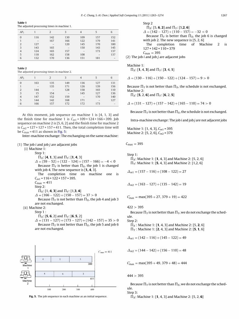
Take a 6 job 2 machine scheduling problem for example.Tables 1 and 2 are the adjusted processing times for machine 1 andmachine 2, respectively. AP25 in Table 1 represents the adjustedprocessing times for job 5 sequenced after job2 in machine 1 witha value of 170. AP25 in Table 2 represents the adjusted process-ing times for job 5 sequenced after job2 in machine 2 with a valueof 165. Different jobs sequenced differently may cause differentprocessing times after taking the setup times into consideration.

An initial sequence of the case example:

Step one: Min{116, 142, 130, 109, 157, 152,163, 135, 149, 136, 127,131,}= 109

The first job to be assigned in machine 1 is job 4.Step two: Min{163, 135, 149, 136, 127, 131}= 127

The first job to be assigned in machine 2 is job 5.

Step three: Again, second job on machine 1 will be job 1.

Second job on machine 2 will be job 6.Step four: The third job on machine one is job 3 and the third jobon machine 2 is job 2.

P.-C. Chang, S.-H. Chen / Applied Soft C

Table 1The adjusted processing times in machine 1.

AP1 1 2 3 4 5 6

0 116 142 130 109 157 1521 – 167 166 122 179 1412 127 – 120 145 170 1803 143 165 – 150 143 1454 124 165 157 – 173 1375 118 162 158 108 – 1376 132 170 136 151 181 –

Table 2The adjusted processing times in machine 2.

AP2 1 2 3 4 5 6

0 163 135 149 136 127 1311 – 135 171 126 139 1562 144 – 128 158 165 1103 15 154 – 145 127 136

tsib

(

4 147 152 159 – 170 1405 144 142 168 171 – 1276 166 157 172 172 173 –

At this moment, job sequence on machine 1 is [4, 1, 3] andhe finish time for machine 1 is Cm1 = 109 + 124 + 166 = 399. Jobequence on machine 2 is [5, 6, 2] and the finish time for machine 2s Cm2 = 127 + 127 + 157 = 411. Then, the total completion time wille Cmax = 411 as shown in Fig. 5:

Inter-machine exchange: The exchanging on the same machine:

1) The job i and job j are adjacent jobs(i) Machine 1:

Step 1:�X: [4, 1, 3] and �Y: [1, 4, 3]

� = (59 − 52) + (122 − 124) + (157 − 166) = −4 < 0Because �Y is better than �X, the job 1 is changed

with job 4. The new sequence is [1, 4, 3].The completion time on machine one is

Cm1 = 116 + 122 + 157 = 395.Cmax = 411Step 2:

�X: [1, 4, 3] and �Y: [1,3, 4]� = (166 − 122) + (150 − 157) = 37 > 0

Because �Y is not better than �X, the job 4 and job 3are not exchanged.

(ii) Machine 2:Step 1 :

�X: [5, 6, 2] and �Y: [6, 5, 2]� = (131 − 127) + (173 − 127) + (142 − 157) = 35 > 0

Because �Y is not better than �X, the job 5 and job 6are not exchanged.

Fig. 5. The job sequence in each machine as an initial sequence.

omputing 11 (2011) 1263–1274 1267

Step 2�X: [5, 6, 2] and �Y: [5,2, 6]

� = (142 − 127) + (110 − 157) = −32 < 0Because �Y is better than �X, the job 6 is changed

with job 2. The new sequence is [5, 2, 6]The completion time of Machine 2 is

127 + 142 + 110 = 379Cmax = 395

(2) The job i and job j are adjacent jobs

Machine 1:�X: [1, 4, 3] and �Y: [3, 4, 1]

� = (130 − 116) + (150 − 122) + (124 − 157) = 9 > 0

Because �Y is not better than �X, the schedule is not exchanged.Machine 2:

�X: [5, 2, 6] and �Y: [6, 2, 5]

� = (131 − 127) + (157 − 142) + (165 − 110) = 74 > 0

Because �Y is not better than �X, the schedule is not exchanged.

Intra-machine exchange: The job i and job j are not adjacent jobs

Machine 1: [1, 4, 3], Cm1 = 395Machine 2: [5, 2, 6], Cm2 = 379

Cmax = 395

Step 1:�X: Machine 1: [1, 4, 3] and Machine 2: [5, 2, 6]�Y: Machine 1: [5, 4, 3] and Machine 2: [1,2, 6]

�m1 = (157 − 116) + (108 − 122) = 27

�m2 = (163 − 127) + (135 − 142) = 19

C ′max = max(395 + 27, 379 + 19) = 422

422 > 395

Because �Y is not better than �Y, we do not exchange the sched-ule.Step 2:

�X : Machine 1: [1, 4, 3] and Machine 2: [5, 2, 6]�Y : Machine 1: [2, 4, 3] and Machine 2: [5, 1, 6]

�m1 = (142 − 116) + (145 − 122) = 49

�m2 = (144 − 142) + (156 − 110) = 48

C ′max = max(395 + 49, 379 + 48) = 444

444 > 395

Because �Y is not better than �X, we do not exchange the sched-ule.Step 3:

�X: Machine 1: [1, 4, 3] and Machine 2: [5, 2, 6]

1 Soft Computing 11 (2011) 1263–1274

u

5

hDhgrwS

5

mttepfiiopsh

Table 3The levels of the population size, crossover rate, and muta-tion rate.

Factors Levels

Population size (PopSize) 100, 200

268 P.-C. Chang, S.-H. Chen / Applied

�Y : Machine 1: [6, 4, 3] and Machine 2: [5,2, 1]

�m1 = (152 − 116) + (151 − 122) = 65

�m2 = (144 − 110) = 34

C ′max = max(395 + 65, 379 + 34) = 460

460 > 395

Because �Y is not better than �X, we do not exchange the sched-le.

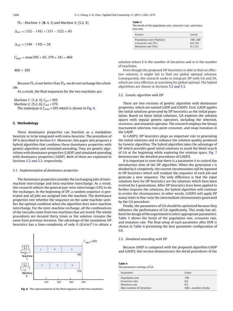
As a result, the final sequences for the two machines are:

Machine 1: [1,4, 3], Cm1 = 395Machine 2: [5,2, 6], Cm2 = 379

The makespan is Cmax = 395 which is shown in Fig. 6.

. Methodology

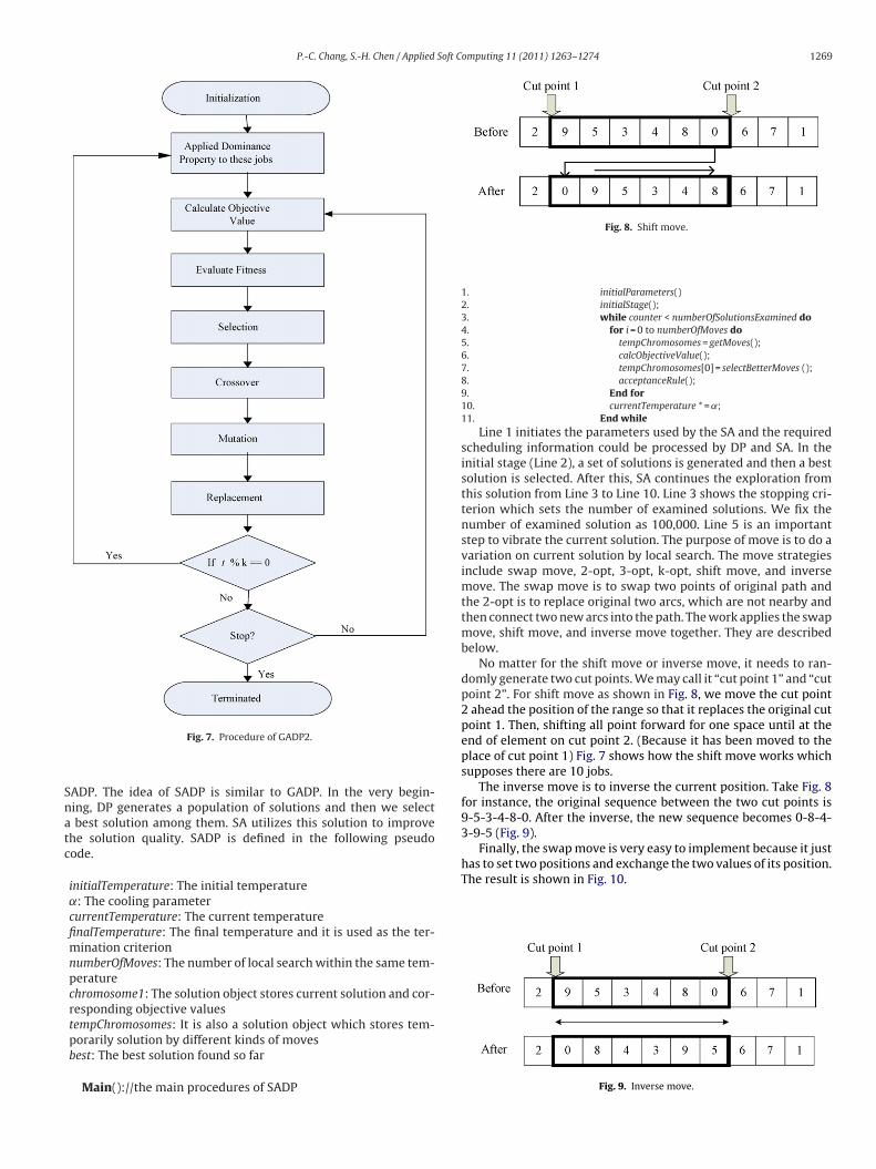
These dominance properties can function as a standaloneeuristic or to be integrated with meta-heuristic. The procedure ofP is described in Section 4.1. Moreover, this paper also proposes aybrid algorithm that combines these dominance properties withenetic algorithm and simulated annealing. They are genetic algo-ithms with dominance properties (GADP) and simulated annealingith dominance properties (SADP). Both of them are explained in

ections 5.2 and 5.3, respectively.

.1. Implementation of dominance properties

The dominance properties consider the exchanging jobs of inter-achine interchange and intra-machine interchange. As a result,

his research utilizes the general pair-wise interchange (GPI) to dohe exchanges. In the beginning of DP, a random sequence is gen-rated and all jobs are assigned into the machine. The dominanceroperties test whether the sequence on the same machine satis-es the optimal condition when the algorithm does inter-machine

nterchange. For the inter-machine exchange, all the combinationsf the two jobs come from two machines that are tested. The wholerocedures are iterated thirty times or the solution remains theame from previous iteration. The advantage of the standalone DPeuristics has a time-complexity of only O (k(n/m)2) to obtain a

Fig. 6. The representation of the final sequence of the two machines.

Crossover rate (Pc) 0.6, 0.9Mutation rate (Pm) 0.1, 0.5

solution where k is the number of iterations and m is the numberof machines.

Even though the proposed DP heuristics is able to find an effec-tive solution, it might fail to find out global optimal solution.Consequently, the research seeks to integrate DP with GA and SA,which are very effective at searching for global optimal. The hybridalgorithms are shown in Sections 5.2 and 5.3.

5.2. Genetic algorithm with DP

There are two versions of genetic algorithm with dominanceproperties, which are named GADP and GADP2. First, GADP appliesthe initial solutions generated by DP heuristics as the initial popu-lation. Based on these initial solutions, GA explores the solutionspaces with regular genetic operators, including the selection,crossover, and mutation operator. The research employs the binarytournament selection, two-point crossover, and swap mutation inthe GADP.

In GADP2, DP heuristics plays an important role in generatingthe initial solutions and to enhance the solution quality producedby Genetic algorithm. The hybrid algorithm takes the advantage ofDP which provides good initial solutions to avoid the blind searchof GA at the beginning while exploring the solution space. Fig. 7demonstrates the detailed procedures of GADP2.

It is important to note that there is a parameter k to control theintroduction time of the DP algorithm. When the generation t isdivided by k completely, the current chromosomes will be inputtedto DP heuristics which will readjust the sequence of each job andgenerate a new sequence. The only difference is that the inputsolutions here for DP heuristics are the solutions which have beenevolved for k generations. After DP heuristics have been applied tofurther improve the solutions, the hybrid algorithm will continueto evolve the chromosomes. In other words, GADP2 will apply DPmany times to fine-tune the intermediate chromosomes generatedby the GA procedure.

Finally, the parameters of GA should be optimized because theyinfluence the performance of GA significantly. This study has uti-lized the design of the experiment to select appropriate parameters.Table 3 shows the levels of the population size, crossover rate,and mutation rate. The final setup of each parameter after DOE isshown in Table 4 presenting the best parameter configuration ofGA.

5.3. Simulated annealing with DP

Because SADP is compared with the proposed algorithm GADPand GADP2, this section demonstrates the detail procedures of the

Table 4The parameter settings of GA.

Parameter Value

Population size 100Crossover rate 0.6Mutation rate 0.5Max number of iterations 500 × number of jobs

P.-C. Chang, S.-H. Chen / Applied Soft Computing 11 (2011) 1263–1274 1269

Snatc

9-5-3-4-8-0. After the inverse, the new sequence becomes 0-8-4-3-9-5 (Fig. 9).

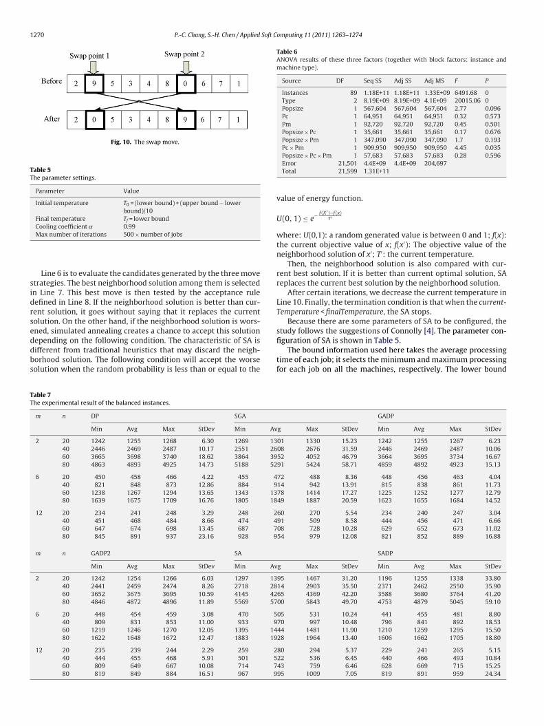
Finally, the swap move is very easy to implement because it justhas to set two positions and exchange the two values of its position.The result is shown in Fig. 10.

Fig. 7. Procedure of GADP2.

ADP. The idea of SADP is similar to GADP. In the very begin-ing, DP generates a population of solutions and then we selectbest solution among them. SA utilizes this solution to improve

he solution quality. SADP is defined in the following pseudoode.

initialTemperature: The initial temperature˛: The cooling parametercurrentTemperature: The current temperaturefinalTemperature: The final temperature and it is used as the ter-mination criterionnumberOfMoves: The number of local search within the same tem-peraturechromosome1: The solution object stores current solution and cor-responding objective values

tempChromosomes: It is also a solution object which stores tem-porarily solution by different kinds of movesbest: The best solution found so far

Main()://the main procedures of SADP

Fig. 8. Shift move.

1. initialParameters()2. initialStage();3. while counter < numberOfSolutionsExamined do4. for i = 0 to numberOfMoves do5. tempChromosomes = getMoves();6. calcObjectiveValue();7. tempChromosomes[0] = selectBetterMoves ();8. acceptanceRule();9. End for10. currentTemperature * = ˛;11. End while

Line 1 initiates the parameters used by the SA and the requiredscheduling information could be processed by DP and SA. In theinitial stage (Line 2), a set of solutions is generated and then a bestsolution is selected. After this, SA continues the exploration fromthis solution from Line 3 to Line 10. Line 3 shows the stopping cri-terion which sets the number of examined solutions. We fix thenumber of examined solution as 100,000. Line 5 is an importantstep to vibrate the current solution. The purpose of move is to do avariation on current solution by local search. The move strategiesinclude swap move, 2-opt, 3-opt, k-opt, shift move, and inversemove. The swap move is to swap two points of original path andthe 2-opt is to replace original two arcs, which are not nearby andthen connect two new arcs into the path. The work applies the swapmove, shift move, and inverse move together. They are describedbelow.

No matter for the shift move or inverse move, it needs to ran-domly generate two cut points. We may call it “cut point 1” and “cutpoint 2”. For shift move as shown in Fig. 8, we move the cut point2 ahead the position of the range so that it replaces the original cutpoint 1. Then, shifting all point forward for one space until at theend of element on cut point 2. (Because it has been moved to theplace of cut point 1) Fig. 7 shows how the shift move works whichsupposes there are 10 jobs.

The inverse move is to inverse the current position. Take Fig. 8for instance, the original sequence between the two cut points is

Fig. 9. Inverse move.

1270 P.-C. Chang, S.-H. Chen / Applied Soft Computing 11 (2011) 1263–1274

Fig. 10. The swap move.

Table 5The parameter settings.

Parameter Value

Initial temperature T0 = (lower bound) + (upper bound − lowerbound)/10

Final temperature Tf = lower bound

sidrseddbs

Table 6ANOVA results of these three factors (together with block factors: instance andmachine type).

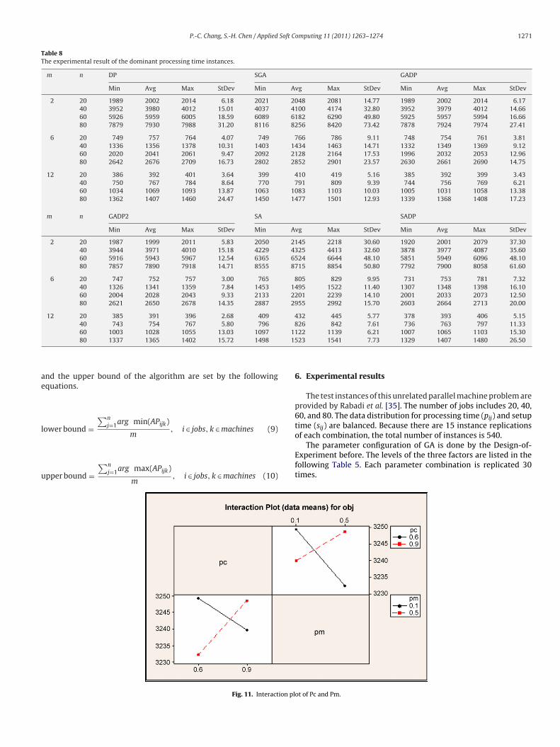
Source DF Seq SS Adj SS Adj MS F P

Instances 89 1.18E+11 1.18E+11 1.33E+09 6491.68 0Type 2 8.19E+09 8.19E+09 4.1E+09 20015.06 0Popsize 1 567,604 567,604 567,604 2.77 0.096Pc 1 64,951 64,951 64,951 0.32 0.573Pm 1 92,720 92,720 92,720 0.45 0.501Popsize × Pc 1 35,661 35,661 35,661 0.17 0.676Popsize × Pm 1 347,090 347,090 347,090 1.7 0.193Pc × Pm 1 909,950 909,950 909,950 4.45 0.035

study follows the suggestions of Connolly [4]. The parameter con-figuration of SA is shown in Table 5.

TT

Cooling coefficient ˛ 0.99Max number of iterations 500 × number of jobs

Line 6 is to evaluate the candidates generated by the three movetrategies. The best neighborhood solution among them is selectedn Line 7. This best move is then tested by the acceptance ruleefined in Line 8. If the neighborhood solution is better than cur-ent solution, it goes without saying that it replaces the currentolution. On the other hand, if the neighborhood solution is wors-ned, simulated annealing creates a chance to accept this solutionepending on the following condition. The characteristic of SA is

ifferent from traditional heuristics that may discard the neigh-orhood solution. The following condition will accept the worseolution when the random probability is less than or equal to the

able 7he experimental result of the balanced instances.

m n DP SGA

Min Avg Max StDev Min Av

2 20 1242 1255 1268 6.30 1269 1340 2446 2469 2487 10.17 2551 2660 3665 3698 3740 18.62 3864 3980 4863 4893 4925 14.73 5188 52

6 20 450 458 466 4.22 455 440 821 848 873 12.86 884 960 1238 1267 1294 13.65 1343 1380 1639 1675 1709 16.76 1805 18

12 20 234 241 248 3.29 248 240 451 468 484 8.66 474 460 647 674 698 13.45 687 780 845 891 937 23.16 928 9

m n GADP2 SA

Min Avg Max StDev Min Av

2 20 1242 1254 1266 6.03 1297 1340 2441 2459 2474 8.26 2718 2860 3652 3675 3695 10.59 4145 4280 4846 4872 4896 11.89 5569 57

6 20 448 454 459 3.08 470 540 809 831 853 11.00 933 960 1219 1246 1270 12.05 1395 1480 1622 1648 1672 12.47 1883 19

12 20 235 239 244 2.29 259 240 444 455 468 5.91 501 560 809 649 667 10.08 714 780 819 849 884 16.51 967 9

Popsize × Pc × Pm 1 57,683 57,683 57,683 0.28 0.596Error 21,501 4.4E+09 4.4E+09 204,697Total 21,599 1.31E+11

value of energy function.

U(0, 1) ≤ e− f (X′)−f (x)T ′

where: U(0,1): a random generated value is between 0 and 1; f(x):the current objective value of x; f(x′): The objective value of theneighborhood solution of x′; T′: the current temperature.

Then, the neighborhood solution is also compared with cur-rent best solution. If it is better than current optimal solution, SAreplaces the current best solution by the neighborhood solution.

After certain iterations, we decrease the current temperature inLine 10. Finally, the termination condition is that when the current-Temperature < finalTemperature, the SA stops.

Because there are some parameters of SA to be configured, the

The bound information used here takes the average processingtime of each job; it selects the minimum and maximum processingfor each job on all the machines, respectively. The lower bound

GADP

g Max StDev Min Avg Max StDev

01 1330 15.23 1242 1255 1267 6.2308 2676 31.59 2446 2469 2487 10.0652 4052 46.79 3664 3695 3734 16.6791 5424 58.71 4859 4892 4923 15.13

72 488 8.36 448 456 463 4.0414 942 13.91 815 838 861 11.7378 1414 17.27 1225 1252 1277 12.7949 1887 20.59 1623 1655 1684 14.52

60 270 5.54 234 240 247 3.0491 509 8.58 444 456 471 6.6608 728 10.28 629 652 673 11.0254 979 12.08 821 852 889 16.88

SADP

g Max StDev Min Avg Max StDev

95 1467 31.20 1196 1255 1338 33.8014 2903 35.50 2371 2462 2550 35.9065 4369 42.20 3588 3680 3764 41.2000 5843 49.70 4753 4879 5045 59.10

05 531 10.24 441 455 481 8.8070 997 10.48 796 841 892 18.5344 1481 11.90 1210 1259 1295 15.5028 1964 13.40 1606 1662 1705 18.80

80 294 5.37 229 241 265 5.1522 536 6.45 440 466 493 10.8443 759 6.46 628 669 715 15.2595 1009 7.05 819 891 959 24.34

P.-C. Chang, S.-H. Chen / Applied Soft Computing 11 (2011) 1263–1274 1271

Table 8The experimental result of the dominant processing time instances.

m n DP SGA GADP

Min Avg Max StDev Min Avg Max StDev Min Avg Max StDev

2 20 1989 2002 2014 6.18 2021 2048 2081 14.77 1989 2002 2014 6.1740 3952 3980 4012 15.01 4037 4100 4174 32.80 3952 3979 4012 14.6660 5926 5959 6005 18.59 6089 6182 6290 49.80 5925 5957 5994 16.6680 7879 7930 7988 31.20 8116 8256 8420 73.42 7878 7924 7974 27.41

6 20 749 757 764 4.07 749 766 786 9.11 748 754 761 3.8140 1336 1356 1378 10.31 1403 1434 1463 14.71 1332 1349 1369 9.1260 2020 2041 2061 9.47 2092 2128 2164 17.53 1996 2032 2053 12.9680 2642 2676 2709 16.73 2802 2852 2901 23.57 2630 2661 2690 14.75

12 20 386 392 401 3.64 399 410 419 5.16 385 392 399 3.4340 750 767 784 8.64 770 791 809 9.39 744 756 769 6.2160 1034 1069 1093 13.87 1063 1083 1103 10.03 1005 1031 1058 13.3880 1362 1407 1460 24.47 1450 1477 1501 12.93 1339 1368 1408 17.23

m n GADP2 SA SADP

Min Avg Max StDev Min Avg Max StDev Min Avg Max StDev

2 20 1987 1999 2011 5.83 2050 2145 2218 30.60 1920 2001 2079 37.3040 3944 3971 4010 15.18 4229 4325 4413 32.60 3878 3977 4087 35.6060 5916 5943 5967 12.54 6365 6524 6644 48.10 5851 5949 6096 48.1080 7857 7890 7918 14.71 8555 8715 8854 50.80 7792 7900 8058 61.60

6 20 747 752 757 3.00 765 805 829 9.95 731 753 781 7.3240 1326 1341 1359 7.84 1453 1495 1522 11.40 1307 1348 1398 16.1060 2004 2028 2043 9.33 2133 2201 2239 14.10 2001 2033 2073 12.5080 2621 2650 2678 14.35 2887 2955 2992 15.70 2603 2664 2713 20.00

12 20 385 391 396 2.68 409 432 445 5.77 378 393 406 5.1540 743 754 767 5.80 796 826 842 7.61 736 763 797 11.33

1115

ae

l

u

60 1003 1028 1055 13.03 109780 1337 1365 1402 15.72 1498

nd the upper bound of the algorithm are set by the followingquations.

ower bound =∑n

j=1arg min(APijk)

m, i ∈ jobs, k ∈ machines (9)

pper bound =∑n

j=1arg max(APijk)

m, i ∈ jobs, k ∈ machines (10)

Fig. 11. Interaction pl

22 1139 6.21 1007 1065 1103 15.3023 1541 7.73 1329 1407 1480 26.50

6. Experimental results

The test instances of this unrelated parallel machine problem areprovided by Rabadi et al. [35]. The number of jobs includes 20, 40,60, and 80. The data distribution for processing time (pij) and setuptime (sij) are balanced. Because there are 15 instance replicationsof each combination, the total number of instances is 540.

The parameter configuration of GA is done by the Design-of-Experiment before. The levels of the three factors are listed in thefollowing Table 5. Each parameter combination is replicated 30times.

ot of Pc and Pm.

1272 P.-C. Chang, S.-H. Chen / Applied Soft Computing 11 (2011) 1263–1274

TT

TA

Fig. 12. Main effect plot of the

able 9he experimental result of the dominant setup time instances.

m n DP SGA

Min Avg Max StDev Min A

2 20 1994 2007 2020 6.38 2023 240 3942 3970 4011 17.01 4031 460 5908 5942 5976 16.39 6073 680 7850 7891 7965 25.27 8102 8

6 20 748 758 766 4.87 75140 1337 1356 1375 8.60 1404 160 2019 2040 2060 9.79 2090 280 2643 2676 2706 15.25 2805 2

12 20 383 390 398 3.58 39840 750 765 783 8.95 76960 1031 1069 1093 14.75 1061 180 1361 1404 1454 21.59 1453 1

m n GADP2 SA

Min Avg Max StDev Min A

2 20 1990 2002 2014 6.02 2030 240 3935 3964 4001 15.67 4203 460 5898 5926 5950 12.25 6376 680 7829 7864 7894 15.62 8519 8

6 20 747 753 759 3.25 76640 1329 1344 1360 7.49 1458 160 2004 2027 2042 9.04 2155 280 2627 2653 2676 12.51 2907 2

12 20 383 388 394 2.66 41440 741 752 765 6.14 79760 1000 1028 1057 13.35 1091 180 1334 1362 1398 15.00 1496 1

able 10NOVA test of the experiment.

Source DF SS

Type 1 2.105E+10Instances 155 2.948E+11Type × instances 155 1.526E+10Method 5 757,891,007Type × method 5 470046.79Instances × method 775 651,513,926Type × instance × method 775 3031145.1Instances × method 775 651,513,926Type × instance × method 775 3031145.1Error 95,328 47,209,017Corrected total 97,199 4.203E+11

three factors of the GA.

GADP

vg Max StDev Min Avg Max StDev

051 2085 14.45 1993 2006 2019 6.21097 4162 32.59 3941 3969 4009 16.66166 6272 51.55 5907 5940 5973 15.97236 8380 69.01 7850 7888 7934 19.99

768 786 8.76 746 754 764 4.84436 1466 14.99 1334 1350 1368 8.40130 2163 17.99 2006 2032 2052 11.09850 2898 22.87 2631 2660 2689 14.07

410 421 5.67 383 389 396 3.26790 808 9.66 743 755 768 6.63082 1102 10.73 1005 1030 1056 12.87478 1502 12.25 1340 1366 1401 15.55

SADP

vg Max StDev Min Avg Max StDev

146 2212 28.70 1927 2005 2086 27.80323 4430 35.10 3889 3970 4066 33.10514 6618 42.10 5830 5932 6023 38.90698 8827 48.20 7734 7875 8002 54.50

806 830 10.35 736 755 783 9.30498 1522 11.90 1315 1349 1392 13.70205 2236 12.30 1991 2032 2072 15.70953 2996 15.30 2606 2666 2717 18.10

432 444 5.17 379 390 414 4.81826 846 7.86 734 760 790 10.61122 1137 6.54 1008 1066 1103 16.30523 1540 7.96 1326 1400 1471 24.50

Mean square F-Value Pr > F

2.105E+10 4.25E+07 <.00011.902E+09 3,840,723 <.000198,428,645 198,755 <.0001151,578,201 306,078 <.000194009.357 189.83 <.0001840663.13 1697.53 <.00013911.155 7.9 <.0001840663.13 1697.53 <.00013911.155 7.9 <.0001495.22718

P.-C. Chang, S.-H. Chen / Applied Soft Computing 11 (2011) 1263–1274 1273

Table 11Duncan pair-wise comparison of these six methods through all instances.

Duncan grouping Mean N Method

A 2435.43 16,200 SAB 2311.14 16,200 SGAC 2206.63 16,200 DPD 2200.37 16,200 SADPE 2195.94 16,200 GADPF 2189.06 16,200 GADP2

Table 12The comparison between GADP2 and PH’s Algorithm.

m n Balanced processing time Dominant processing time Dominant setup time

LB GADP2 PH’s Algorithm LB GADP2 PH’s Algorithm LB GADP2 PH’s Algorithm

2 20 1186 1254 1296 1933 1999 2046 1936 2002 205040 2345 2459 2521 3844 3971 4019 3834 3964 403160 3510 3675 3733 5767 5943 5997 5755 5926 598080 4665 4872 4927 7672 7890 7933 7649 7864 7914

6 20 362 454 480 613 752 779 611 753 77640 717 831 848 1214 1341 1361 1218 1344 137160 1071 1246 1232 1823 2028 1965 1822 2027 196980 1429 1648 1626 2426 2650 2673 2428 2653 2670

ttuPabfuF

SAmtimwpFTe

eac

AotcbcG

cGa

12 20 175 239 250 30040 347 455 473 59760 519 649 627 89480 690 849 830 1191

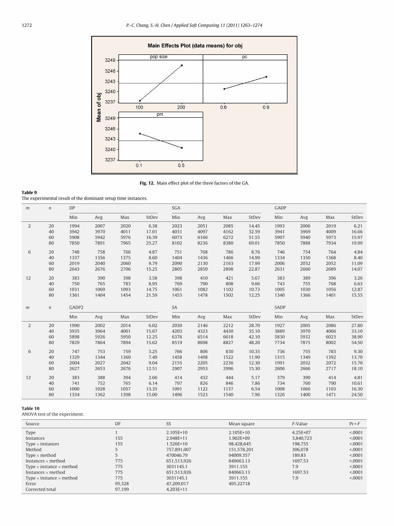
When we examine the significance of these factors, the ANOVAable as shown in Table 6 indicates that there is significant betweenhe crossover rate and mutation rate. Consequently, we furtherse the interaction plot in Fig. 11 to select the setting of Pc andm. We found when we set the crossover rate and mutation ratet the level 0.6 and 0.5, respectively; the algorithm will yield aetter solution quality. Because there is no significant differenceor population size when they are set as 100 and 200, the pop-lation size is set as the 100 based on the main effect plot inig. 12.

This research compares the performance of DP heuristics, GA,A, GADP, GADP2, SADP, and Partition Heuristic Algorithm. PH’slgorithm is proposed by Al-Salem [35] in solving the parallelachines scheduling problems. There are three heuristics sequen-

ially applied in the PH algorithm to minimize the makespan,ncluding the constructive, improvement, and a traveling sales-

an problem (TSP)-like heuristic. Constructive is the first heuristichich assigns the jobs to machines. Secondly, an improvementrocedure is used to improve the previous constructed solution.inally, similar to the heuristic of traveling salesman problem, aSP-like heuristic is applied, which sets the sequence of jobs onach machine.

The following Tables 7–9 are the empirical result of the differ-nt types of instances. DP heuristic performs the best among theselgorithms such as GA, SA and DP. Moreover, when GA and SA areombined with DP, the overall performances are further enhanced.

In order to validate the significance among these algorithms,NOVA is employed to test it, which shows significant differencesf these factors in Table 10. The Duncan pair-wise comparisonests the significance among these methods in Table 11. The Dun-an grouping presents each algorithm located in different groupecause they share different alphabet. As a result, there is statisti-al significance between any two algorithms. The best algorithm is

ADP2, the second best is GADP, and the worst is SA.

Finally, because GADP2 is the best among all algorithms, it isompared with PH’ algorithm again. As shown in Table 12, we foundADP2 outperforms PH’s algorithm consistently except the job setsre 60 and 80 on machine 6 and 12.

391 402 299 388 398754 769 597 752 769

1028 986 894 1028 9901365 1348 1192 1362 1357

7. Conclusions and future direction of research

The problem addressed in this paper is referred to the unrelatedparallel machine scheduling problem (PMSP) with machine-dependent and sequence-dependent setup times to minimize themakespan. This research derives the dominance properties forunrelated parallel machine scheduling problem. According to theempirical results, the proposed DP heuristic outperforms GA andSA in effectiveness (the solution quality) and efficiency (less com-putational time). Moreover, DP heuristics can be integrated withmeta-heuristic and the hybrid algorithm is a novel approach in solv-ing the scheduling problems. GADP is able to find optimal solutionsfor all small problems. For large problems, GADP when comparedto GA, SA and GADP still outperforms the other two approaches innearly all instances.

It will be interesting to extend this work by including localheuristic such as PH algorithm in GADP and investigate whethermore improvement can be further accomplished. Or, solutions fromthese combinations of different heuristics can be injected into thepopulation during the evolution of the GA. Benchmark data setsand solutions for both heuristics used in this paper are made avail-able in our website for other researchers to compare their solutionmethodologies.

References

[1] Allahverdi, J.N.D. Gupta, T. Aldowaisan, A review of scheduling research involv-ing setup considerations, Omega 27 (2) (1999) 219–239.

[3] M. Asano, H. Ohta, A heuristic for job shop scheduling to minimize totalweighted tardiness, Computers and Industrial Engineering 42 (2–4) (2002)137–147.

[4] P. Brucker, S. Knust, A. Schoo, O. Thiele, A branch and bound algorithm for theresource-constrained project scheduling problem, European Journal of Opera-tional Research 107 (2) (1998) 272–288.

[5] P.C. Chang, J.C. Hsieh, Y.W. Wang, Genetic algorithms applied in BOPP filmscheduling problems: minimizing total absolute deviation and setup times,Applied Soft Computing 3 (2) (2003) 139–148.

[6] P.C. Chang, S.H. Chen, K.L. Lin, Two phase sub-population genetic algorithm forparallel machine scheduling problem, Expert Systems with Applications 29 (3)(2005) 705–712.

1 Soft C

[

[

[

[

[

[

[

[

[

[

[

[

[

[

[

[

[

[

[

[

[

[

[

[

[

[

[

[

886–894.[39] K.-C. Tan, R. Narasimhan, P.A. Rubin, G.L. Ragatz, A Comparison of four methods

274 P.-C. Chang, S.-H. Chen / Applied

[7] P.C. Chang, J.C. Hsieh, C.H. Liu, A case-injected genetic algorithm for singlemachine scheduling problems with release time, International Journal of Pro-duction Economics 103 (2) (2006) 551–564.

[8] P.C. Chang, J.C. Hsieh, C.Y. Wang, Adaptive multi-objective genetic algorithmsfor scheduling to drilling operation of printed circuit board industry, AppliedSoft Computing Journal 7 (3) (2007) 800–806.

[9] P.C. Chang, S.-H. Chen, C.-Y. Fan, Mining gene structures to inject artificial chro-mosomes for genetic algorithm in single machine scheduling problems, AppliedSoft Computing Journal 8 (1) (2008) 767–777.

10] P.C. Chang, S.H. Chen, The development of a sub-population genetic algorithmII (SPGAII) for the Multi-objective combinatorial problems, Applied Soft Com-puting Journal 9 (1) (2009) 173–181.

11] P.C. Chang, T.W. Liao, Combining SOM and fuzzy rule base for flow time pre-diction in semiconductor manufacturing factory, Applied Soft Computing 6 (2)(2006) 198–206.

12] F.D. Chou, P.C. Chang, H.M. Wang, A hybrid genetic algorithm to minimizemakespan for the single batch machine dynamic scheduling problem, Inter-national Journal of Advanced Manufacturing Technology 31 (3/4) (2006)350–359.

13] D.T. Connolly, An improved annealing scheme for the quadratic assignmentproblems, European Journal of Operational Research 46 (1) (1990) 93–100.

14] S. Dunstall, A. Wirth, Heuristic methods for the identical parallel machine flowtime problem with set-up times, Computers and Operations Research 32 (9)(2005) 2479–2491.

15] P.M. Franca, M. Gendreau, G. Laporte, F.M. Müller, A tabu search heuristic forthe multiprocessor scheduling problem with sequence dependent setup times,International Journal of Production Economics 43 (2/3) (1996) 79–89.

16] M.R. Garey, D.S. Johnson, Computers and Intractability: A Guide to the Theoryof NP-Completeness, W. H. Freeman & Co., New York, NY, USA, 1979.

17] M. Ghirardi, C.N. Potts, Makespan minimization for scheduling unrelated par-allel machines: a recovering beam search approach, European Journal ofOperational Research 165 (2) (2005) 457–467.

18] C.A. Glass, C.N. Potts, P. Shade, Unrelated parallel machine scheduling usinglocal search, Mathematical and Computer Modelling 20 (2) (1994) 41–52.

19] S.C. Graves, A review of production scheduling, Operations Research 29 (4)(1981) 646–675.

20] A. Guinet, A. Dussauchy, Scheduling sequence-dependent jobs on identical par-allel machines to minimize completion time criteria, International Journal ofProduction Research 31 (1993) 1579–1594.

21] J.C. Hsieh, P.C. Chang, L.C. Hsu, Scheduling of drilling operations in printed-circuit-board factory, Computers and Industrial Engineering 44 (3) (2003)461–473.

22] D.W. Kim, K.H. Kim, W. Jane, F.F. Chen, Unrelated parallel machine schedulingwith setup times using simulated annealing, Robotics and Computer IntegratedManufacturing 18 (3/4) (2002) 223–231.

[

omputing 11 (2011) 1263–1274

23] D.W. Kim, D.G. Na, F.F. Chen, Unrelated parallel machine scheduling with setuptimes and a total weighted tardiness objective, Robotics and Computer Inte-grated Manufacturing 19 (1/2) (2003) 173–181.

24] S.C. Kim, P.M. Bobrowski, Scheduling jobs with uncertain setup times andsequence dependency, Omega 25 (4) (1997) 437–447.

25] M.E. Kurz, R.G. Askin, Heuristic scheduling of parallel machines with sequence-dependent set-up times, International Journal of Production Research 39 (16)(2001) 3747–3769.

26] G. Lancia, Scheduling jobs with release dates and tails on two unrelated parallelmachines to minimize the Makespan, European Journal of Operational Research120 (2) (2000) 277–288.

27] C.Y. Liaw, Y.K. Lin, C.Y. Chen, M. Chen, Scheduling unrelated parallel machinesto minimize total weighted tardiness, Computers & Operations Research 30(12) (2003) 1777–1789.

28] Y. Lin, W. Li, Parallel machine scheduling of machine-dependent jobs with unit-length, European Journal of Operational Research 156 (1) (2004) 261–266.

29] C.Y. Liu, S.C. Chang, Scheduling flexible flow shops with sequence-dependentsetup effects, IEEE Transactions on Robotic Automation 16 (4) (2000) 408–429.

30] S. Martello, F. Soumis, P. Toth, Exact and approximation algorithms forMakespan minimization on unrelated parallel machines, Discrete AppliedMathematics 75 (2) (1997) 169–188.

31] H. Missbauer, Order release and sequence-dependent setup times, Interna-tional Journal of Production Economics 49 (2) (1997) 131–143.

32] E. Mokotoff, Parallel machine scheduling problems: a survey, Asia-Pacific, Jour-nal of Operational Research 18 (2) (2001) 193–242.

33] J.-C. Picard, M. Queyranne, On the integer-valued variables in the linear vertexpacking problem, Mathematical Programming 12 (1) (1977) 97–101.

34] M. Pinedo, Scheduling: Theory, Algorithms, and Systems, Prentice Hall, NJ,1995.

35] G. Rabadi, R.J. Moraga, A. Al-Salem, Heuristics for the unrelated parallel machinescheduling problem with setup times, Journal of Intelligent Manufacturing 17(1) (2006) 85–97.

36] S. Radhakrishnan, J.A. Ventura, Simulated annealing for parallel machinescheduling with earliness-tardiness penalties and sequence-dependent set-uptimes, International Journal of Production Research 38 (10) (2000) 2233–2252.

38] B. Srivastava, An effective heuristic for minimizing makespan on unrelatedparallel machines, Journal of the Operational Research Society 49 (8) (1998)

for minimizing total tardiness on a single processor with sequence dependentsetup times, Omega 28 (3) (2000) 313–326.

40] R. Zhang, C. Wu, A hybrid immune simulated annealing algorithm for the jobshop scheduling problem, Applied Soft Computing 10 (1) (2010) 79–89.