Embed Size (px)
Citation preview
DOKUZ EYLÜL UNIVERSITY
GRADUATE SCHOOL OF NATURAL AND APPLIED
SCIENCES
INTEGRATION OF ACTIVE VIBRATION
CONTROL METHODS WITH FINITE ELEMENT
MODELS OF SMART STRUCTURES
by
Levent MALGACA
May, 2007
İZMİR
INTEGRATION OF ACTIVE VIBRATION
CONTROL METHODS WITH FINITE ELEMENT
MODELS OF SMART STRUCTURES
A Thesis Submitted to the Graduate School of Natural and Applied Sciences of
Dokuz Eylül University In Partial Fulfillment of the Requirements for the
Degree of Doctor of Philosophy in Mechanical Engineering,
Machine Theory and Dynamics Program
by
Levent MALGACA
May, 2007
İZMİR
ii
Ph.D. THESIS EXAMINATION RESULT FORM
We have read the thesis entitled “INTEGRATION OF ACTIVE VIBRATION
CONTROL METHODS WITH FINITE ELEMENT MODELS OF SMART
STRUCTURES” completed by Levent MALGACA under supervision of Prof. Dr.
Hira KARAGÜLLE and we certify that in our opinion it is fully adequate, in scope
and in quality, as a thesis for the degree of Doctor of Philosophy.
Supervisor
Thesis Committee Member Thesis Committee Member
Examining Committee Member Examining Committee Member
Prof. Dr. Cahit HELVACI
Director
Graduate School of Natural and Applied Sciences
Prof. Dr. Hira KARAGÜLLE
Prof. Dr. A. Saide SARIGÜL Yrd. Doç. Dr. Zafer DİCLE
Prof. Dr. Yavuz YAMAN Prof. Dr. Mustafa SABUNCU

iii
ACKNOWLEDGEMENTS
I would like to thank my supervisor, Prof. Dr. Hira KARAGÜLLE for his very
valuable guidance, his support and his critical suggestions throughout my doctoral
studies. It was a privilege to study under his supervision.
I am grateful to the members of my doctoral committee, Prof. Dr. A. Saide
SARIGÜL and Assist. Prof. Dr. Zafer DİCLE, for their careful review and advice
during the research.
I would also like to thank my colleagues, Assist. Prof. Dr. Zeki KIRAL, Research
Assistant Murat AKDAĞ and Burcu GÜNERI for their inspiration.
Finally, I wish to express special thanks to dear my wife, TÜLAY for her
encouragement, patience and love during this doctoral work. My thanks also to my
son, ARDA, who makes everything worthwhile.
I wish to dedicate this thesis to my parents who have always supported to me.
Levent MALGACA
İzmir, 2007
iv
INTEGRATION OF ACTIVE VIBRATION CONTROL METHODS WITH
FINITE ELEMENT MODELS OF SMART STRUCTURES
ABSTRACT
Active control methods can be used to eliminate undesired vibrations in
engineering structures. Using piezoelectric smart structures for the active vibration
control has great potential in engineering applications. In this thesis, numerical and
experimental studies on active vibration control of mechanical systems and smart
structures have been presented.
An integrated analysis procedure has been developed for the control of structures.
The closed loop control laws are incorporated into the finite element (FE) models by
using ANSYS parametric design language (APDL). The proposed procedure is first
tested by applying to multi degrees of freedom mechanical systems. Then, active
control of free and forced vibrations of piezoelectric smart beams in different
configurations is studied with this procedure. The control gains and piezoelectric
actuation voltages which provide vibration control are determined by the numerical
simulations. Harmonic excitation and moving load problems are considered in the
forced vibration control. The active vibration suppression is achieved using strain
feedback and displacement feedback
Experiments have been conducted to verify the closed loop simulations. Smart
beams consist of aluminum beams (450 mm x 20 mm x 1.5 mm, 1000 mm x 20 mm
x 1.5 mm) surface bonded piezoelectric patches of Sensortech BM532 (25 mm x 20
mm x 1 mm) and strain gages. The natural frequencies of cantilever smart beams are
found using chirp signals. Experimental results are obtained by LabVIEW programs
developed in the study. It is observed that theoretical predictions are well matched
with the experimental results.
Keywords: Active vibration control, piezoelectric smart structures, closed loop-
finite element analysis.
v
AKILLI YAPILARIN SONLU ELEMAN MODELLERİ İLE AKTİF
TİTREŞİM KONTROL YÖNTEMLERİNİN BÜTÜNLEŞTİRİLMESİ
ÖZ
Mühendislik yapılarındaki istenmeyen titreşimleri yok etmek için aktif kontrol
yöntemleri kullanılabilir. Mühendislik uygulamalarındaki aktif titreşim kontrolü için
piezoelektrik akıllı yapıların kullanımı önemli potansiyele sahiptir. Bu tezde,
mekanik sistemlerin ve akıllı yapıların aktif titreşim kontrolü üzerine sayısal ve
deneysel çalışmalar sunulmuştur.
Yapıların kontrolü için bir entegre analiz yöntemi geliştirildi. Bu yöntemde,
ANSYS parametrik tasarım dili kullanılarak, sonlu eleman modelleri ile kapalı devre
kontrol kuralları bütünleştirilmiştir. Önerilen yöntem, önce çok serbestlik dereceli
mekanik sistemlere uygulanarak test edilir. Sonra farklı konfigürasyonlardaki
piezoelektrik akıllı kirişlerin serbest ve zorlanmış titreşimlerinin kontrolü bu
yöntemle ile çalışılır. Kontrol kazançları ve titreşim kontrolünü sağlayan kumanda
voltajları sayısal simülasyonlar ile belirlenir. Zorlanmış titreşim kontrolünde,
harmonik uyarı ve hareketli yük problemleri dikkate alınır. Aktif titreşim kontrolü
şekil değiştirme geri beslemesi ve yer değiştirme geri besleme kullanarak elde edilir.
Kapalı devre simulasyonları doğrulamak amacı ile deneyler yürütüldü. Akıllı
kirişler, alüminyum kirişlerin (450 mm x 20 mm x 1.5 mm, 1000 mm x 20 mm x 1.5
mm) üzerine yapıştırılmış Sensortech BM532 tip piezoelektrik yamalar (25 mm x 20
mm x 1 mm) ve uzama ölçerlerden oluşur. Ankastre akıllı kirişlerin doğal
frekansları, sinüzoidal sinyaller kullanılarak belirlenir. Deneysel sonuçlar bu
çalışmada geliştirilen LabVIEW programları ile elde edilir. Teorik tahminlerin
deneysel sonuçlar ile iyi bir şekilde eşleştiği gözlemlenir.
Anahtar sözcükler: Aktif titreşim kontrolü, piezoelektrik akıllı yapılar, kapalı
devre- sonlu eleman analizi.
vi
CONTENTS
Page
THESIS EXAMINATION RESULT FORM...………………………………………ii
ACKNOWLEDMENTS……..………………………………………………………iii
ABSTRACT…………………………………………………………………………iv
ÖZ………………………………………………………………………………….....v
CHAPTER ONE – INTRODUCTION AND LITERATURE REVIEW..............1
1.1 Introduction……………………………………………………………………1
1.1.1 The Finite Element Bibliography………………………………………...1
1.1.2 Active Vibration Control of Smart Structures……………………………4
1.1.3 Scope of the Research….……………………………………………….12
1.1.4 Organization of the Thesis..……………………….……………………13
CHAPTER TWO - INTEGRATION OF ACTIVE VIBRATION CONTROL
METHODS WITH THE FINITE ELEMENT MODELS OF MECHANICAL
SYSTEMS…………………………………………………………………………..15
2.1 Introduction…………………………………………………………………..15
2.2 Active Vibration Control in Multi-DOF Mass-Spring System.....…………...16
2.2.1 Analytical Solution……………………………………………………...17
2.2.2 Solution by The Runge-Kutta Method…………………...……………..20
2.2.3 Closed Loop Simulation by ANSYS……………….…………………...23
2.2.4 Integrated Approach Solution…………………………………………..25
CHAPTER THREE - ANALYSIS OF ACTIVE VIBRATION CONTROL IN
SMART STRUCTURES BY ANSYS…………………………………………….31
3.1 Introduction…………………………………………………………………..31
vii
3.2 A Two-Degrees of Freedom System..………………………………………..31
3.2.1 Analytical Solution……………………………………………………...31
3.2.2 Closed Loop Simulation by ANSYS……………………………………35
3.3 Active Vibration Control in Smart Structures….…………………………….36
3.3.1 Beam Type Structures..…………….……………………………….......37
3.3.2 Smart Circular Disc..................................................................................45
3.3.3 Smart Plate...............................................................................................48
3.4 Characteristics of Vibration Signals...……………………………….……….54
CHAPTER FOUR – EXPERIMENTAL ANALYSIS OF ACTIVE
VIBRATION CONTROL IN SMART STRUCTURES AND COMPARISON
WITH CLOSED LOOP - FINITE ELEMENT SIMULATIONS……..………..55
4.1 Introduction…………………………………………………………………..55
4.2 Experimental System.......................................................................................55
4.3 Closed Loop Simulation..…………………………………………………….63
4.4 Comparison of Experimental and Simulation Results……………………….68
4.4.1 Modal Analysis...…………………………………………………….68
4.4.2 Active Control of Free Vibrations…………………………………...70
4.4.2.1 Strain Feedback Control………………………………………..70
4.4.2.2 Displacement Feedback Control………………………………..75
CHAPTER FIVE - SIMULATION AND EXPERIMENTAL ANALYSIS OF
ACTIVE VIBRATION CONTROL OF SMART BEAMS UNDER
HARMONIC EXCITATION……………………………………………………...81
5.1 Introduction…………………………………………………………………..81
viii
5.2 Active Control of Forced Vibrations…………………………………………81
5.2.1 Structural Modeling…………………………………………………….82
5.2.2 Simulation…………….………………………………………………...84
5.2.3 Experiment........………………………………………………………...88
5.3 Simulation and Experimental Results..………………………………………90
5.3.1 Strain Feedback Control….......................................................................90
5.3.2 Displacement Feedback Control………………………………………...91
CHAPTER SIX – ANALYSIS OF ACTIVE VIBRATION CONTROL OF
SMART BEAMS SUBJECTED TO MOVING LOAD………...……………....100
6.1 Introduction…………………………………………………………………100
6.2 Vibration Analysis of a Beam Subjected to Moving Load………………....103
6.2.1 Experiments……………………………………………………………103
6.2.2 The Finite Element Simulation………………………….……………..108
6.2.3 Experimental and Simulation Results…………………………………109
6.3 Active Vibration Control of Smart Beams Subjected to Moving Load…….130
6.3.1 A Cantilever Smart Beam with Two Piezo-actuators.…………………130
6.3.2 A Fixed-Fixed Smart Beam with Multiple Piezo-actuators………..….143
6.3.2.1 Moving Load Formulations and Parameters..…………………….145
6.3.2.2 Closed Loop Simulation………………………………………….146
CHAPTER SEVEN – RESULTS AND DISCUSSIONS……………………….156
CHAPTER EIGHT – CONCLUSIONS………………………………………...159
REFERENCES……………………………………………………………………162
APPENDICES…………………………………………………………………….170

ix
A - SMART MATERIALS AND STRUCTURES...............................................170
B - THE COMPUTER CODES DEVELOPED BY LABVIEW………………189
C - THE COMPUTER CODES DEVELOPED BY APDL FOR CLOSED
LOOP SIMULATIONS…………………………………………………………..193
1
CHAPTER ONE
INTRODUCTION AND LITERATURE REVIEW
1.1 Introduction
It is desired to design lighter mechanical systems carrying out higher work loads at
higher speeds. However, the vibration may become prominent factor in this case. Active
control methods can be used to eliminate the undesired vibration. Using piezoelectric
smart structures for the active vibration control is paid considerable attention in the last
decade. In this chapter, a bibliographical review of the FE models applied to the analysis
and simulation of smart materials and structures is summarized. Previous theoretical and
experimental studies performed in active vibration control of smart structures are
reviewed. Scope of the research and organization of the thesis are also presented in this
chapter. Smart materials studied in the literature, the piezoelectric finite element method
and the piezoelectric constitutive equations are summarized in Appendix A.
1.1.1 The Finite Element Bibliography
The FE method is used for the study of the coupled electromechanical response of
various smart materials; also the sensor and actuator functions of smart structures in
practice is simulated by the FE technique and often also compared with experiments.
A bibliographical review of the FE method applied to the analysis and simulation of
smart materials and structures is presented by Mackerle (2003). The review of published
papers dealing with the FE method applied to smart materials and structures is given in
the study. Theoretical aspects as well as design and practical implementations are
covered. The lists of references of papers published between 1997–2002 are divided into
the following sections and subsections: smart materials, smart components and
structures, smart sensors and actuators, controlled structures technology.
2
The bibliography is organized in two main parts. In the first one, current trends in
modeling techniques are mentioned. The second part contains a list of papers published
in the period of 1997–2002. A similar study is also presented in the period of 1986-1998
(Mackerle, 1998).
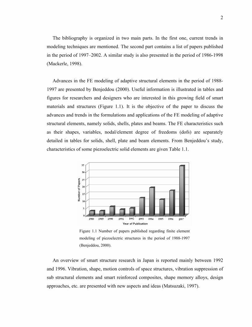
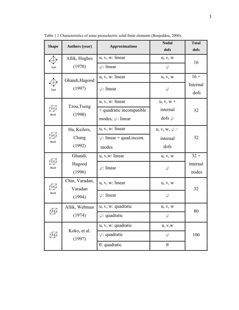
Advances in the FE modeling of adaptive structural elements in the period of 1988-
1997 are presented by Benjeddou (2000). Useful information is illustrated in tables and
figures for researchers and designers who are interested in this growing field of smart
materials and structures (Figure 1.1). It is the objective of the paper to discuss the
advances and trends in the formulations and applications of the FE modeling of adaptive
structural elements, namely solids, shells, plates and beams. The FE characteristics such
as their shapes, variables, nodal/element degree of freedoms (dofs) are separately
detailed in tables for solids, shell, plate and beam elements. From Benjeddou’s study,
characteristics of some piezoelectric solid elements are given Table 1.1.
An overview of smart structure research in Japan is reported mainly between 1992
and 1996. Vibration, shape, motion controls of space structures, vibration suppression of
sub structural elements and smart reinforced composites, shape memory alloys, design
approaches, etc. are presented with new aspects and ideas (Matsuzaki, 1997).
Figure 1.1 Number of papers published regarding finite element
modeling of piezoelectric structures in the period of 1988-1997
(Benjeddou, 2000).
3
Table 1.1 Characteristics of some piezoelectric solid finite elements (Benjeddou, 2000).
Shape Authors (year) Approximations Nodal
dofs
Total
dofs
u, v, w: linear u, v, w
Allik, Hughes
(1970) f: linear f 16
u, v, w: linear u, v, w
Ghandi,Hagood
(1997) f: linear f
16 +
Internal
dofs
u, v, w: linear
Tzou,Tseng
(1990) + quadratic incompatible
modes, f: linear
u, v, w +
internal
dofs f 32
u, v, w: linear
Ha, Keilers,
Chang
(1992)
f: linear + quad.incom.
modes
u, v, w, f+
internal
dofs
32
u, v,w: linear u, v, w
Ghandi,
Hagood
(1996) f: linear f
32 +
internal
nodes
u, v, w: linear u, v, w
Chin, Varadan,
Varadan
(1994) f: linear f 32
u, v, w: quadratic u, v, w
Allik, Webman
(1974) f: quadratic f 80
u, v, w: quadratic u, v,w
f: quadratic f Koko, et al.
(1997) θ: quadratic θ
100
4
1.1.2 Active Vibration Control of Smart Structures
The active vibration control of cantilever beams and plates is studied in the literature
by mounting piezoelectric patches as actuators on the beams and plates. Another
piezoelectric patch or a strain gage can be used to sense the vibration level. Kim, V. V.
Varadan, V. K. Varadan & Bao (1996) studied the FE modeling of an aluminum
cantilever beam instrumented with piezoelectric actuator and sensor. Piezoelectric
elements are modeled with three-dimensional 20-node brick element while beam
structure is modeled with 9-node shell element. 13-node transition element is used to
connect the three-dimensional solid elements to the flat-shell elements. Lim, Varadan &
Varadan (1997, 1999) investigated vibration controllability of beams with piezoelectric
sensors and actuators using the FE analysis in both frequency and time domain. They
showed the suppression of vibration amplitudes with both constant displacement and
velocity feedback. The sensor response is examined when a unit voltage is applied to the
actuator. Celentano & Setola (1999) developed a simplified model of beam-like
structure with bonded piezoelectric plate by integrating usual electrical with the FE
method and mechanical models with a RLC circuit.
Manning, Plummer & Levesley (2000) presented a smart structure vibration control
scheme using system identification and pole placement technique. System identification
is carried out in three phases: data collection, model characterization and parameter
estimation. Input-output data are collected by stimulating the piezoelectric actuators with
a square wave signal and monitoring the strain gage response. Negative velocity
feedback is used as the controller to reduce vibration amplitudes. Gaudenzi, Carbonaro
& Benzi (2000) investigated this problem both experimentally and numerically with
position and velocity control approaches. The numerical simulation is developed with
the FE method based on an Euler-Bernoulli model. A single input-output feedback
closed loop control system is used for the solution. When numerical simulation and
experimental tests are compared, it is reported that a good agreement is obtained for the
cases where position control is more effective than velocity control to reduce the
5
vibration level in a cantilever beam. Bruant, Coffignal, Lene, & Verge (2001) presented
by modeling beam structures contained piezoelectric devices with a simple finite
composite element. A three beam and a simple cantilever beam structures are studied.
Six mechanical degrees of freedom and four electric degrees of freedom are used in the
model. They developed a methodology for the determination of the optimal geometries
of piezoelectric devices. Halim & Moheimani (2002) aimed to develop a feedback
controller that suppresses vibration of flexible structures. The controller (Hinf) is applied
to a simple-supported PZT laminate beam and it is validated experimentally.
Gabbert, Trajkov & Köppe (2002) studied design and simulation of controlled smart
plate using a state-space model of a plate obtained through the FE analysis as a starting
point for the controller design. For the purpose of the control design for the vibration
suppression, LQ optimal controller is used. The FE analysis is used by COSAR which is
a general purpose FE-package while control design is realized by
MATLAB/SIMULINK. Singh, Pruthi & Agarwal (2003) also used the beam and piezo-
patches the FE model, but applied modal control strategies. Electro-dynamic modeling
of the system is done using the FE formulation Euler beam elements. The vibration
response of the beam to an impulse excitation is calculated numerically for the
uncontrolled and controlled cases. The analytical results are evaluated comparing with
the modal control strategies. Lin & Nyang (2003) discussed the effectiveness of different
feedback control methods by means of the FE analysis by comparing numerical results,
obtained using the FE method, and experimental results.
Kusculuoglu, Fallahi & Roston (2004) developed a new FE model for a beam with a
piezoceramic patch actuator. Each layer is treated as a Timoshenko beam. Two
experimental studies are validated the theoretical developments. They observed that the
use of the introduced model became more important when the piezoceramic and base
layer thickness were large and shear and related rotational inertia became more
important. Fei (2005) investigated active vibration control methods with strain feedback
6
controller for a cantilever beam bonded piezoelectric actuators. The optimized PID
compensator is implemented experimentally using xPC Target real time system.
Vasques & Rodrigues (2006) presented an analysis and comparison of the classical
control strategies (constant amplitude and constant velocity feedback) and optimal
control strategies (linear quadratic regulator and linear quadratic Gaussian controller) on
the active vibration control of piezoelectric smart beams under initial displacement field
and white noise force disturbance. The following conclusions are pointed out in their
study. The advantage of the classical techniques is that they can avoid the necessity of
digital control reducing the time delays and providing stability. However, noisy
measurements can become troublesome for these strategies due to the necessity of the
differentiation of the sensor voltage. The optimal control techniques have various
performance criteria. A major limitation of the LQR is that all states must be measured
when generating control. The LQG control overcomes that by estimating the states using
a Kalman-Bucy filter.
In the active control of piezoelectric smart structures, it is possible to improve the
control performance of the system and to minimize energy consumption if actuators are
placed at optimal locations (Bruant et al., 2001, Quek, Wang & Ang, 2003, Xu & Koko,
2004, Peng, Ng & Hu, 2005). Peng et al. (2005) developed a performance criterion for
the optimization of PZT patch locations on a thin cantilever rectangular plate. The
parameters of the actuator location are determined by ANSYS. Genetic Algorithm is
used to implement the optimization. The control performance is evaluated with a
filtered-x LMS based multi-channel adaptive control. Lim (2003) studied the vibration
control of several modes of a clamped square plate by locating discrete sensor/actuator
devices at points of maximum strain. Constant velocity and constant displacement
control algorithms are used through the closed loop control. It is concluded that discrete
sensors/actuators should be preferred over piezoelectric films to realize lower weight
and effective control authority for modest values of actuator voltages for active vibration
control of practical structures. PZT actuators can also be used for precision positioning
7
applications. Ma & Nejhad (2005) presented an adaptive control scheme for
simultaneous precision positioning and vibration suppression of intelligent structures.
Two PID feedback and two adaptive feedforward controllers are experimentally studied
on the active composite plates under harmonic and random disturbances. The two
adaptive controllers are employed, one precision positioning and the other vibration
suppression.
Flexible structures are subjected to various dynamic excitations in many engineering
fields such as civil engineering, aerospace engineering and mechanical engineering.
Engineers aim to eliminate vibrations that occur due to dynamic excitations. Vibration
levels of smart structures under continuous excitation can be reduced with active control.
Fariborzi, Golnaraghi & Heppler (1997) experimentally developed energy-based control
strategy linear coupling control (LCC) for controlling forced vibrations in flexible
structures. MATLAB software is used to implement the control law. Choi, Park &
Fukuda (1998) investigated the active control of hybrid smart structures under forced
vibrations. Two hybrid smart structures considered in the study include PZT
film/electro-rheological fluid actuators and piezoceramic/shape memory alloy actuators.
Jha & Rower (2002) performed an experimental study on active vibration control
using neural network and PZT actuators. Control performance of a cantilever plate is
tested with sine wave and white noise disturbances. Yaman et al. (2003) investigated
experimentally a μ synthesis active vibration control technique applied to the sinusoidal
forced vibrations of a smart fin. They designed controllers for both SISO (Single-Input
Single-Output) and SIMO (Single-Input Multi-Output) system models and presented
results in the frequency domain. Vibrations are suppressed through LabVIEW based
programs. Kumar and Singh (2006) dealt with the inverted L structure with two PZT
actuators and sensor for forced vibration attenuation. One of the actuators is the
disturbance source. They obtained better transient performance with adaptive hybrid
control by combining the feedback and feed forward controllers for a large range of
excitation frequencies.
8
Integration of composite materials and piezoelectric sensor/actuators is considered as
an ideal candidate especially in aerospace applications (Yaman et al., 2003). Wang,
Quek & Ang (2001) studied on the vibration control of smart composite plates by means
of the FE analysis and negative velocity feedback method. Raja & Sihna (2002) studied
active vibration control of a composite sandwich beam with two kinds of piezoelectric
actuator such as extension-bending and shear. They derived the FE formulation using
quasi-static equations of piezoelectricity and developed a control scheme based on the
linear quadratic regulator/independent modal space control method. It is reported that
the shear actuator is more efficient in controlling the first three bending modes than the
extension-bending actuator. Quek et al. (2003) presented an optimal placement strategy
of piezoelectric sensor/actuator pairs for the vibration control of laminated composite
plates. Yang & Liu (2005) presented a feedforward adaptive controller based on an
adaptive filter for system dynamics identification of composite laminated smart
structures with experimental verifications. Experimental results show that adaptive
control is effective for vibration suppression of smart structures. Baillargeon & Vel
(2005) also presented vibration suppression of adaptive sandwich cantilever beam using
PZT shear actuators by experiments and numerical simulations. The beam is
harmonically excited at its fundamental frequency by a stack actuator attached to the tip.
The control system with positive position feedback and strain rate feedback is
implemented by MATLAB/Simulink and a dSPACE digital controller. Moita, Soares &
Soares (2005) dealt with a FE formulation for active control of forced vibrations of thin
plate/shell laminated structures with integrated PZT layers, based on third-order shear
deformation theory. They used the Newmark method to calculate the dynamic response
under forced vibration. Yang, Sheu & Liu (2005) presented adaptive filter design for
system dynamics identification of composite laminated smart structures developing a
feedforward adaptive controller based on an adaptive filter with dynamic convergence
for vibration suppression. Both the adaptive filter for system identification and the
adaptive controller for vibration suppression are implemented in TMS320C32 digital
signal processor for real-time applications.
9
The demands for high speed performance and low energy consumption are main
motivation for the lightweight robot manipulators in mechanical engineering
applications. Smart structures are also used in robot applications. Fung &Yau (2004)
investigated the vibration control of a clamped free rotating flexible cantilever arm with
active constrained layer damping (ACLD) treatment. Hamilton’s principle with the FE
method is used to derive closed loop equation of motions neglecting the gravitational
and rotary inertia effects in the model. PD controller is designed for the PZT sensor and
actuator. The effects of different rotating speed, thickness ratio and different controller
gain on the damping frequency and damping ratio are presented.
Sun, Mills, Shan and Tsoa (2004) proposed a new approach for the use of a PZT
actuator to control a single-link flexible manipulator. A combined scheme of PD
feedback and command voltages applied to segmented PZT actuators is investigated for
rigid motion control as well as vibration damping. The PZT actuator control is employed
linear velocity feedback that makes the algorithm easy to implement. Simulation and
experimental results confirmed these theoretical predictions. Wang & Mills (2005)
studied a dynamic model for a general planar flexible linkage by using the Lagrange-FE
formulation. The nonlinear coupling of rigid body motion and flexible motion and the
linear electromechanical coupling are integrated in the model. Active vibration control
simulation results of strain rate feedback control using PZT sensors and actuators are
given.
Ge, Lee & Gong (1999) proposed a flexible SCARA Cartesian robot system
combined with piezoelectric materials. Subsequently dynamic modeling and controller
design are investigated. Directly based on the partial differential equations (PDEs)
model a novel distributed controller is developed. Both simulation and experimental
results are verified that the robust controller can achieve good performance in the
suppression of residual vibrations under the environment of disturbances. Shin & Choi
(2001) presented mixed actuator scheme to actively control the end point position of a
two-link manipulator. A highly nonlinear system model including inertial effect is
10
established using Lagrange's equation associated with assumed mode method. Control
scheme consists of four actuators; two-servomotors at the hubs and two piezoelectric
elements attached to the surfaces of the flexible links. The effectiveness of proposed
methodology both regulating and tracking control responses is evaluated through
experimental realization. Kim, Choi & Thompson (2001) also examined motion control
(position and force) of a two-link flexible manipulator accomplished by employing
servomotors mounted at the hub and piezoceramic actuators bonded on each link. The
governing equations of motion of the smart manipulator are derived via Hamilton's
principle. A set of sliding mode controller with perturbation estimation is formulated for
the actuators. The routine is then incorporated with the fuzzy technique to determine the
appropriate control gains. Xianmin, Changjian & Erdman (2002) studied the active
vibration control in a four-bar linkage. A pair of PZT actuator and sensor is bonded on
each of the links. The FE model is used and the reduced mode, standard H∞, and robust
H∞ control strategies are analyzed. It is discussed that the vibration of the system is
significantly suppressed with permitted control voltages by each of these controllers.
Smart structures can be modeled and simulated with high accuracy using powerful
computers and commercial FE-packages such as ANSYS, ABAQUS and
MSC/NASTRAN. The simulation results play important role in understanding and
examining the dynamic behaviour of the system before physical experiments are
realized. Computer simulations enable to rerun many times with minimal cost and to
change parameters of the analysis after the FE model is constructed. Experiments should
also be performed to validate the FE model proposed in simulations. The procedure is
presented for modeling structures containing PZT actuators using MSC/NASTRAN and
MATLAB (Reaves & Horta, 2003). The cantilever smart beam is modeled by
MSC/NASTRAN. MATLAB scripts are used to assemble the dynamic equation and
generate frequency response functions from deflection and strain data as a function of
input voltage to the actuator. Xu & Koko (2004) reported results using the commercial
FE-package ANSYS. The optimal control design is carried out in the state space form
established on the FE modal analysis and applied to cantilever smart beam and clamped
11
smart plate structures. MATLAB Control System Toolbox for the control design is used
in their study. The influence of sensor/actuator location is studied. They observed that
the location near to the clamped end was better for the vibration control. Seba, Ni &
Lohmann (2006) studied a numerical model of a beam structure with PZT actuator
obtained in the ANSYS-MATLAB platform for vibration attenuation. The model is
validated by experiments using shunting circuits by means of the FE analysis
optimization. The analysis is extended to a chassis subframe of a car as a complex
structure in both the experiment and ANSYS.
Karagülle, Malgaca & Öktem (2004) realized the integration of control actions into
ANSYS modeling and solutions. Firstly, the procedure is tested on the active control
problem with a two-degrees of freedom system. The analytical results obtained by the
Laplace transform method are compared to ANSYS results. Then, the smart structures
are studied with the same procedure. The results obtained using the integrated procedure
are compared with the results of structures analyzed in other reference studies.
Therefore, the FE modeling and control actions are carried out together by ANSYS.
Dong, Meng & Peng (2006) used the same procedure by incorporating the control
law into the ANSYS-FE model to perform closed loop simulations with (LQG)
controller. The efficiency of a system identification technique known as
observer/Kalman filter identification (OKID) technique is investigated in the numerical
simulation and experimental study of active vibration control of piezoelectric smart
structures. Based on the structure responses determined by the FE method, an explicit
state space model of the equivalent linear system is developed by employing OKID
approach. The similar objective to develop a general design and analysis scheme for
actively controlled PZT smart structures is presented by Meng, Dong & Wei (2006). In
order to perform closed loop simulations, the LQG control law is incorporated into the
FE model by ANSYS. The scheme involves dynamic modeling of a smart structure by
designing control laws and closed loop simulation in the FE environment.
12
1.1.3 Scope of the Research
Nowadays, FE models of complex mechanical systems can be constructed rapidly in
many engineering programs. Users of commercial FE programs such as ANSYS can
analyze systems by defining their systems and the inputs. These programs develop the
mathematical model of the systems and perform their solutions. It is possible to extract
the mathematical models from the FE programs and then it can be used in conjunction
with other commercial control programs such as MATLAB to solve closed loop
problems. By incorporating the control law directly into the FE programs, the closed
loop control problems with complex structures can be analyzed more easily.
The main motivation of this research is to develop general design and analysis
scheme by incorporating the control law directly into the FE programs. The closed loop
control law is incorporated into the FE models by using APDL. The FE analysis with
closed loop control actions are carried out by ANSYS. Closed loop-FE simulations of
piezoelectric smart structures are performed with this procedure developed in the thesis.
The control gains and vibration controlling piezoelectric actuation voltages are
determined by the simulations before experiments are conducted.
The FE models of smart structures such as beam, circular disc and rectangular plate
are constructed by ANSYS. Closed loop-FE simulations of these smart structures are
studied with the integrated procedure to reduce vibration amplitudes. Active control of
free and forced vibrations of smart beams is achieved using strain and displacement
feedbacks. In free and forced vibration control, smart beams having different
configurations are considered. Active control of forced vibrations in smart beams is
analyzed under harmonic excitation and moving load. The experiments are performed to
verify these simulation results.
13
1.1.4 Organization of the Thesis
This thesis consists of eight chapters (including the introduction and the conclusions)
and the appendices.
Chapter 1 presents literature survey of the related research, scope and organization of
the thesis. A bibliographical review of FE method applied to the analysis and simulation
of smart structures is presented. Previous studies on active vibration control of
piezoelectric smart structures are reviewed.
In chapter 2, the integration of active vibration control methods with FE models of
mechanical systems is presented. Analysis of active vibration control of a 3-DOF mass-
spring system is studied with four different methods. Analytical, numerical, closed loop
simulations by ANSYS and integrated approach solutions are realized. In the first
method, analytical solution of the system excited by a step input from the base is found
by the Laplace method. Secondly, the closed loop control of the system which has a
mathematical model in state variable format is examined by the Runge-Kutta method.
Thirdly, the control law is incorporated into the ANSYS-FE model to perform closed
loop simulations. In the last method, control part is performed in MATLAB/Simulink
after the FE matrices of the system are extracted from ANSYS. The integrated approach
and closed loop-FE solutions are the original works developed in the thesis.
Chapter 3 presents closed loop-FE simulations of smart structures. The closed loop
control law is incorporated into ANSYS-FE model by using APDL. First, the procedure
is tested on the active vibration control problem with two-degrees of freedom system.
The analytical results obtained by the Laplace transform method, and the simulation
results by ANSYS are compared. Then, the smart structures studied in references are
analyzed. The results are obtained for the structures analyzed in other studies. The active
vibration control of a circular disc and a square plate are also studied.
14
In chapter 4, experiments are conducted to verify closed loop simulation results. The
closed loop control law can be incorporated into ANSYS-FE model as mentioned in the
previous chapter. The control gains and vibration controlling piezoelectric actuation
voltages can be determined by the simulations. Active control of free vibration of the
smart beam included a piezoelectric actuator and a strain gage is considered in this
chapter. The experimental system is introduced. Experimental modal analysis is
performed applying chirp signals to the piezoelectric actuator. Active control of the
smart beam is achieved by applying both strain and displacement feedback. Control OFF
and Control ON vibration signals are obtained for various gains.
Chapter 5 presents the active control of a smart beam under forced vibration as both
simulation and experimental. The configuration of the smart beam is different from the
beam considered in the previous chapter. Active vibration reduction under harmonic
excitation is achieved using both strain and displacement feedback control. The
simulation and experimental time responses of the beam are evaluated as the
performance criteria.
In chapter 6, experimental vibration analysis of a cantilever aluminum beam
subjected to moving load is presented at first. Experimental system for moving load is
introduced. Experimental results are compared with the simulation results obtained by
ANSYS. Then, active vibration control of smart beams under moving load is studied
with the simulations using strain and displacement feedback controls. Two case studies
are presented to demonstrate the validity of the analysis procedure proposed in the
thesis.
Finally, the results, the conclusions and the suggestions for future works in closed
loop-FE simulations of smart structures or other mechanical systems are presented.
Appendices present smart materials and structures, the computer codes of the
simulations and the experimental works developed in the thesis.
15
CHAPTER TWO
INTEGRATION OF ACTIVE VIBRATION CONTROL METHODS WITH
FINITE ELEMENT MODELS OF MECHANICAL SYSTEMS
2.1 Introduction
Active vibration control can be applied to various structures in different
engineering fields such as aerospace engineering (Ülker et al., 2005), civil
engineering (Seto & Matsumato, 1999) and mechanical engineering (Xianmin et al.,
2002, O’Connor & Lang, 1998). O’Connor & Lang (1998) proposed to model a
single link flexible robot arm as lumped parameter multi-degrees of freedom system.
Active control is applied to the system using wave absorption technique. The
position control of flexible robot arms is achieved with a fast response time and a
minimum of residual vibration.
It is possible to model complex mechanical systems by computer programs using
the FE method. The dynamic responses are obtained if the inputs are defined to the
programs. The values of responses are found in the programs by using numerical
methods. The values of inputs are given for a time interval with a time step, and the
values of the responses are found for the same time interval with the same time step.
In this chapter, the integration of the control strategies to these programs is
considered. The integration of the closed loop control strategies of a flexible
mechanical system of which dynamic model can be solved with different methods is
considered.
Analysis of active vibration control of a 3-DOF mass-spring system is performed
with analytical solution, the Runge-Kutta method, closed loop simulation using
ANSYS and integrated approach. Damping is ignored to demonstrate the
effectiveness of the active control. The dynamic response of the displacement of the
last mass at the tip is evaluated as performance criteria for various gains of PID
control. The results obtained by the four different methods are compared to each
other for the system excited by a step input from the base.
16
In the first method, analytical solution is found by the Laplace method after the
equations of motion for the system are obtained. Secondly, the closed loop control of
a system which has a mathematical model in state variable format is examined by the
Runge-Kutta method. Beginning with the first values of the mathematical system,
PID control requirements are performed to the instantaneous error values solved by
the Runge-Kutta method. Thirdly, close loop simulations are performed in ANSYS
by integrating control actions into the FE model. In the last method, integrated
approach is studied. Control part is performed in MATLAB/Simulink after mass and
stiffness matrices of the system are extracted from ANSYS. The FE matrices are
written to an output file in ANSYS. These matrices in Harwell-Boeing format are
converted to mass and stiffness matrices by a MATLAB program.
2.2 Active Vibration Control in Multi-DOF Mass-Spring System
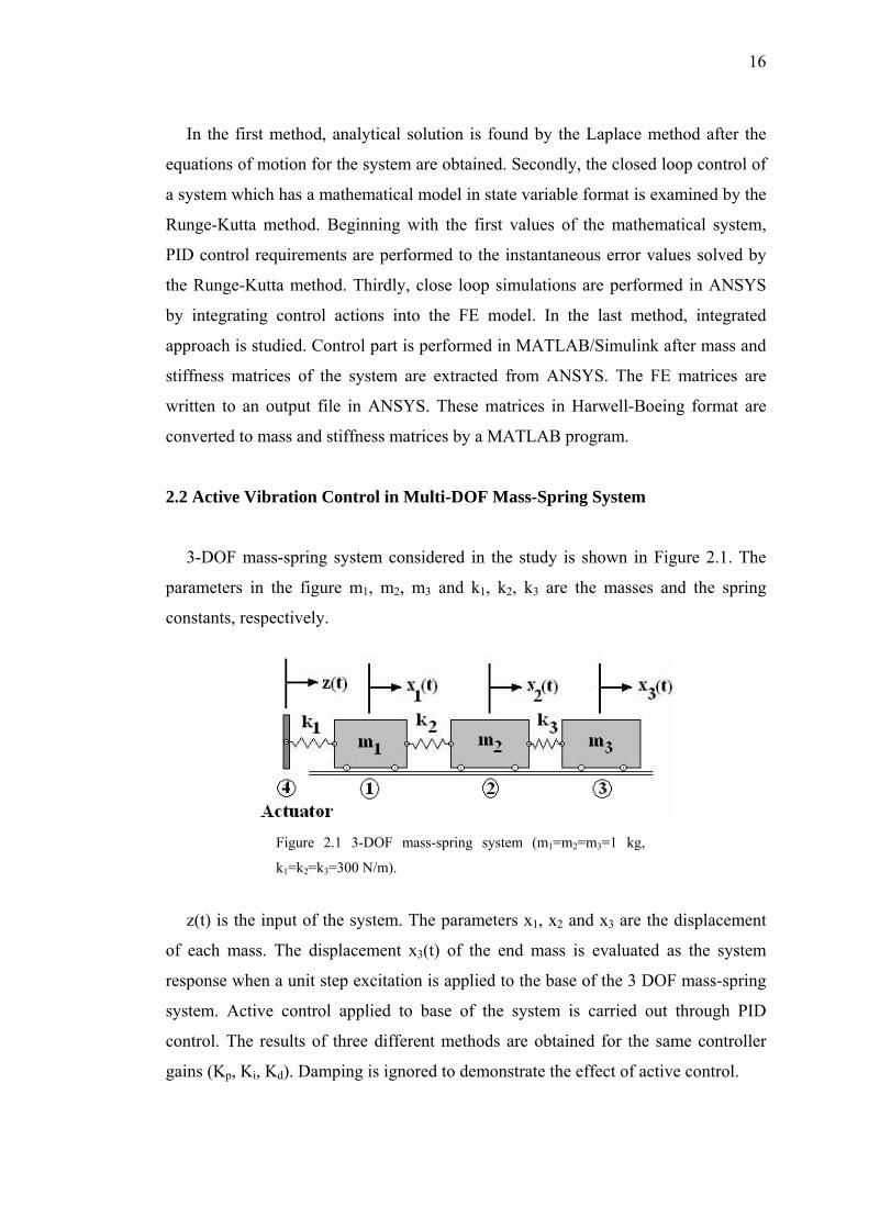
3-DOF mass-spring system considered in the study is shown in Figure 2.1. The
parameters in the figure m1, m2, m3 and k1, k2, k3 are the masses and the spring
constants, respectively.
z(t) is the input of the system. The parameters x1, x2 and x3 are the displacement
of each mass. The displacement x3(t) of the end mass is evaluated as the system
response when a unit step excitation is applied to the base of the 3 DOF mass-spring
system. Active control applied to base of the system is carried out through PID
control. The results of three different methods are obtained for the same controller
gains (Kp, Ki, Kd). Damping is ignored to demonstrate the effect of active control.
Figure 2.1 3-DOF mass-spring system (m1=m2=m3=1 kg,
k1=k2=k3=300 N/m).
17
2.2.1 Analytical Solution
The equation of motion for undamped multi-degrees of freedom vibrating system
is given as
[ ]{ } [ ]{ } { }fxKxM =+••
(2.1)
where M, K and f are the mass, stiffness and force matrices, respectively. The
parameter x is the general coordinate. After the kinetic and potential energies of the
system considered are found, the equations of motion are obtained applying
Lagrange equation and written in matrix format as follows;
)t(z00k
xxx
kk0kkkk0kkk
x
x
x
m000m000m 1
321
333322
221
3
2
1
32
1
⎪⎭
⎪⎬⎫
⎪⎩
⎪⎨⎧
=⎪⎭
⎪⎬⎫
⎪⎩
⎪⎨⎧
⎥⎥
⎦
⎤
⎢⎢
⎣
⎡
−−+−
−++
⎪⎪⎪
⎭
⎪⎪⎪
⎬
⎫
⎪⎪⎪
⎩
⎪⎪⎪
⎨
⎧
⎥⎥
⎦
⎤
⎢⎢
⎣
⎡
••
••
••
(2.2)
If x(t)=Xiest, z(t)=0, natural frequencies of the system are calculated by
substituting numerical values in Equation (2.2).
⎪⎭
⎪⎬⎫
⎪⎩
⎪⎨⎧
=⎪⎭
⎪⎬⎫
⎪⎩
⎪⎨⎧
⎥⎥⎥
⎦
⎤
⎢⎢⎢
⎣
⎡
+−−+−
−+
000
XXX
300s3000300600s3000300600s
321
A
22
2
44444 344444 21
(2.3)
If det(A)=0, s6+1500s4+540000s2+27000000=0 (2.4)
ω1 = 7.7084 (rad/s) → f1 = 1.2268 (Hz)
ω2 = 21.5983 (rad/s) → f2 = 3.4375 (Hz)
ω3 = 31.2105 (rad/s) → f3 = 4.9673 (Hz)
18
Applying the Laplace Transform method to Equation (2.2), Equation (2.5) is
written in order to find the transfer functions. If the input is z(t)= est and the response
is x(t)=H(s) est.
⎪⎭
⎪⎬
⎫
⎪⎩
⎪⎨
⎧
⎥⎥⎥
⎦
⎤
⎢⎢⎢
⎣
⎡
+++++++
+++=
⎪⎭
⎪⎬
⎫
⎪⎩
⎪⎨
⎧
00
)s(Zk
270000s1200s)600s(30090000)600s(300180000s900s)300s(300
90000)300s(30090000s900s
)s(D1
)s(X)s(X)s(X 1
242
2242
224
3
2
1
The transfer function of the open loop system in Figure 2.1 is found to be;
)s(D27000000
)s(Z)s(3X)s(HOL == (2.6)
If F(s)=k1Z(s), Z(s)=1/s, the transfer functions between the input Z(s) and Xi(s) can
be found as the following,
X1(s) = H11(s).F(s), X2(s) = H12(s).F(s), X3(s) = H13(s).F(s)
)s(D90000s9004s)s(H
211
++= (2.7)
)s(D90000s300)s(H
212
+= (2.8)
)s(D90000)s(H13 = (2.9)
Utilizing the block diagram in Figure 2.2, then the transfer function of the closed
loop system is found to be;
U(s)={Xr(s)-K[X1(s)+X2(s)+X3(s)]} (2.10)
(2.5)
19
X1(s) = uH11(s), X2(s) = uH12(s), X3 (s)= uH13(s) (2.11)
[ ])s(H)s(H)s(H)s(H)s(X)s(KG)s(G)s(x
)s(H)s(X
13121113
311r
13
3 ++−= (2.12)
[ ])s(H)s(H)s(H)s(KG1)s(G)s(H
)s(X)s(X)s(H
1312111
113
r
3CL +++
== (2.13)
Substituting Xr(s)=1 and the values of the transfer functions,
i66
p
6i
3p
43
4id
45p
6d
7ip
2d
6
3
K10x27s)10x27K106x27(
s)10x27K104x12(s)K10x1210x540(
s)K100K10x12(s)K1001500(sK100s)KsKsK(10x27
)s(X
2
+++
++++
+++++
++= (2.14)
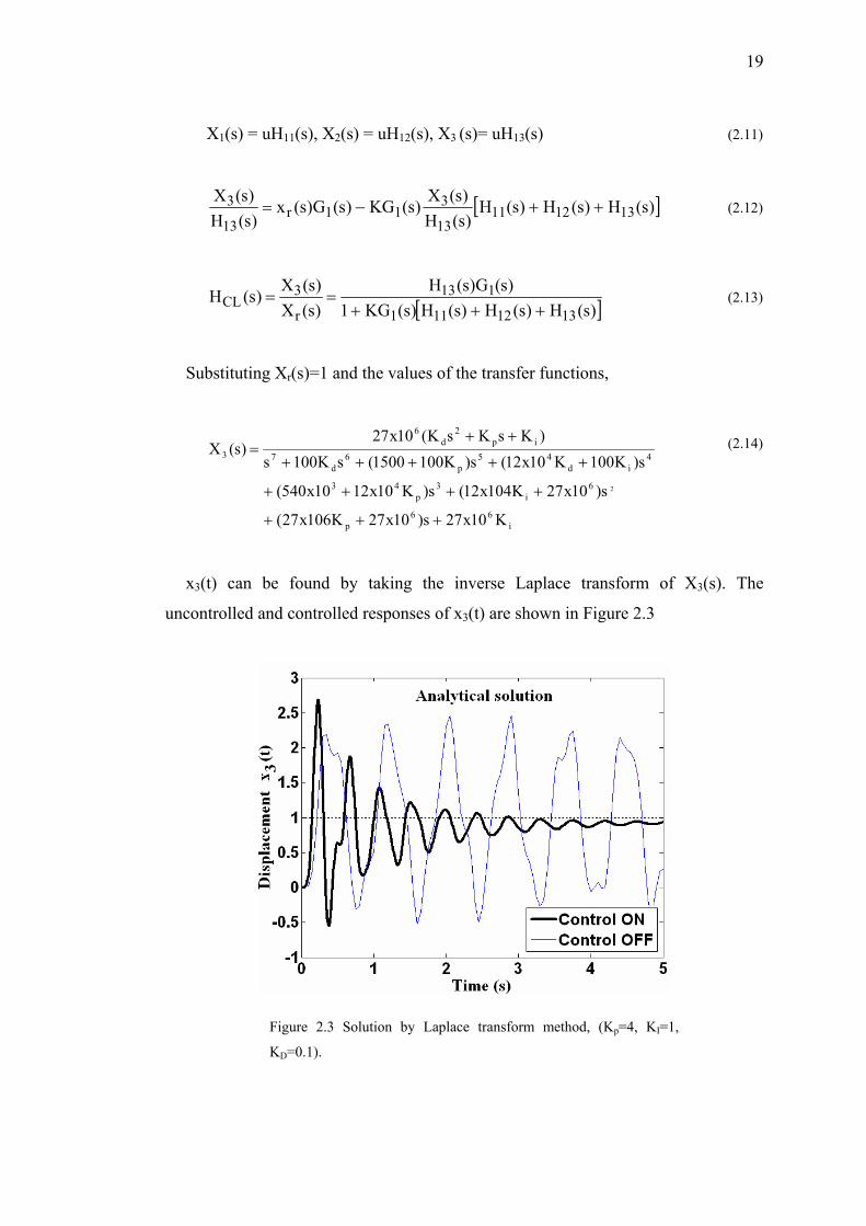
x3(t) can be found by taking the inverse Laplace transform of X3(s). The
uncontrolled and controlled responses of x3(t) are shown in Figure 2.3
Figure 2.3 Solution by Laplace transform method, (Kp=4, KI=1,
KD=0.1).
20
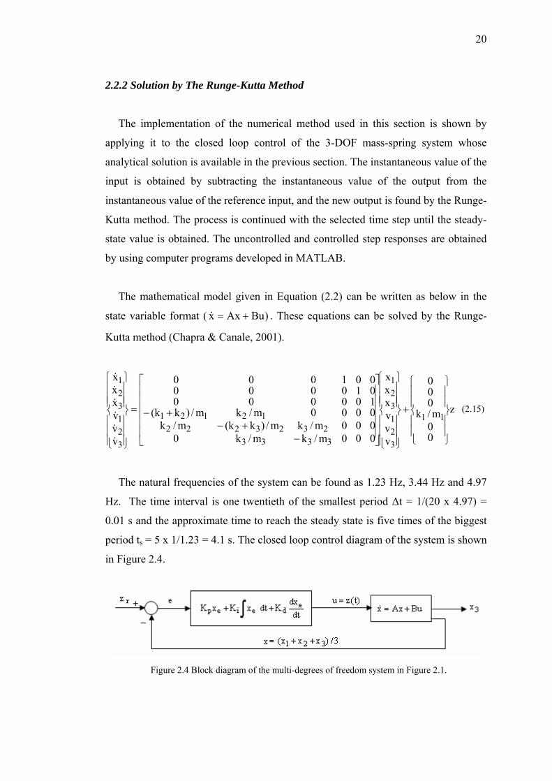
2.2.2 Solution by The Runge-Kutta Method
The implementation of the numerical method used in this section is shown by
applying it to the closed loop control of the 3-DOF mass-spring system whose
analytical solution is available in the previous section. The instantaneous value of the
input is obtained by subtracting the instantaneous value of the output from the
instantaneous value of the reference input, and the new output is found by the Runge-
Kutta method. The process is continued with the selected time step until the steady-
state value is obtained. The uncontrolled and controlled step responses are obtained
by using computer programs developed in MATLAB.
The mathematical model given in Equation (2.2) can be written as below in the
state variable format ( )BuAxx +=& . These equations can be solved by the Runge-
Kutta method (Chapra & Canale, 2001).
z
00m/k
000
vvvxxx
000m/km/k0000m/km/)kk(m/k0000m/km/)kk(100000010000001000
vvvxxx
11
321321
33332323222
12121
321321
⎪⎪
⎭
⎪⎪
⎬
⎫
⎪⎪
⎩
⎪⎪
⎨
⎧
+
⎪⎪⎪
⎭
⎪⎪⎪
⎬
⎫
⎪⎪⎪
⎩
⎪⎪⎪
⎨
⎧
⎥⎥⎥⎥⎥
⎦
⎤
⎢⎢⎢⎢⎢
⎣
⎡
−+−
+−=
⎪⎪⎪
⎭
⎪⎪⎪
⎬
⎫
⎪⎪⎪
⎩
⎪⎪⎪
⎨
⎧
&&&&&&
(2.15)
The natural frequencies of the system can be found as 1.23 Hz, 3.44 Hz and 4.97
Hz. The time interval is one twentieth of the smallest period Δt = 1/(20 x 4.97) =
0.01 s and the approximate time to reach the steady state is five times of the biggest
period ts = 5 x 1/1.23 = 4.1 s. The closed loop control diagram of the system is shown
in Figure 2.4.
Figure 2.4 Block diagram of the multi-degrees of freedom system in Figure 2.1.
21
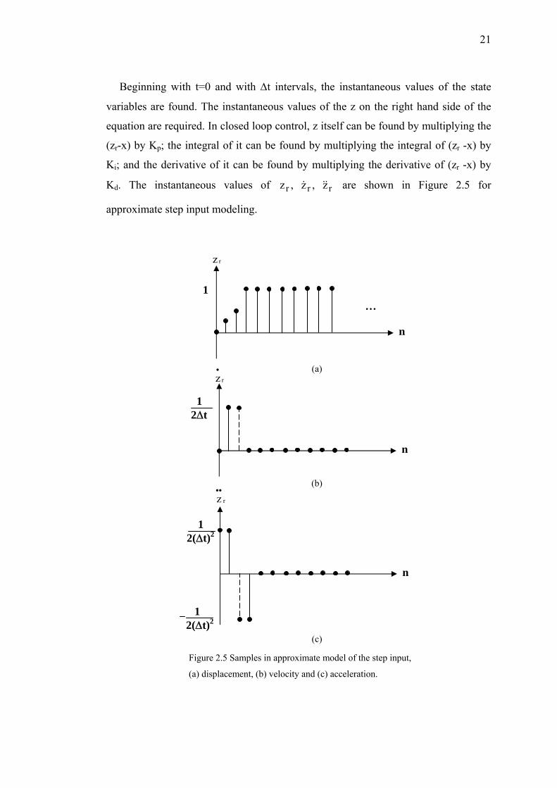
Beginning with t=0 and with Δt intervals, the instantaneous values of the state
variables are found. The instantaneous values of the z on the right hand side of the
equation are required. In closed loop control, z itself can be found by multiplying the
(zr-x) by Kp; the integral of it can be found by multiplying the integral of (zr -x) by
Ki; and the derivative of it can be found by multiplying the derivative of (zr -x) by
Kd. The instantaneous values of rrr z,z,z &&& are shown in Figure 2.5 for
approximate step input modeling.
Figure 2.5 Samples in approximate model of the step input,
(a) displacement, (b) velocity and (c) acceleration.
(a)
(b)
(c)
n
1 2(Δt)2
1 2(Δt)2
rz••
n
1 2Δt
rz•
n
1 …
rz
22
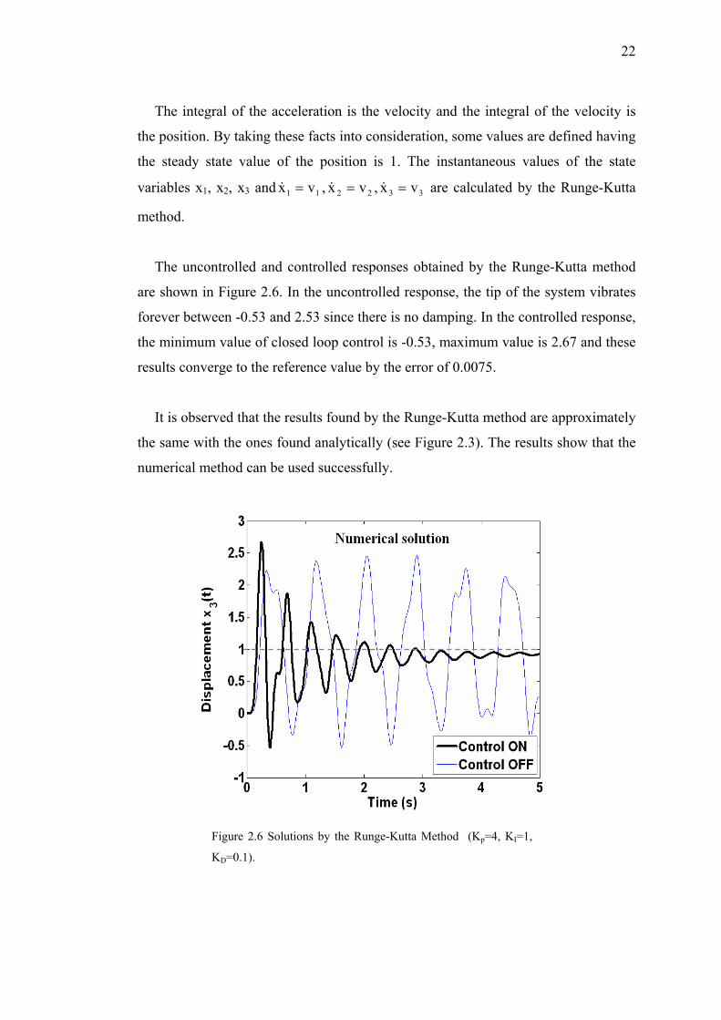
The integral of the acceleration is the velocity and the integral of the velocity is
the position. By taking these facts into consideration, some values are defined having
the steady state value of the position is 1. The instantaneous values of the state
variables x1, x2, x3 and 11 vx =& , 22 vx =& , 33 vx =& are calculated by the Runge-Kutta
method.
The uncontrolled and controlled responses obtained by the Runge-Kutta method
are shown in Figure 2.6. In the uncontrolled response, the tip of the system vibrates
forever between -0.53 and 2.53 since there is no damping. In the controlled response,
the minimum value of closed loop control is -0.53, maximum value is 2.67 and these
results converge to the reference value by the error of 0.0075.
It is observed that the results found by the Runge-Kutta method are approximately
the same with the ones found analytically (see Figure 2.3). The results show that the
numerical method can be used successfully.
Figure 2.6 Solutions by the Runge-Kutta Method (Kp=4, KI=1,
KD=0.1).
23
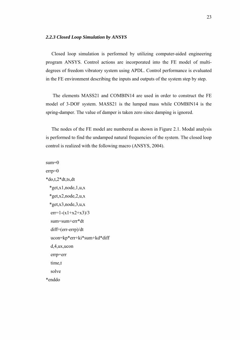
2.2.3 Closed Loop Simulation by ANSYS
Closed loop simulation is performed by utilizing computer-aided engineering
program ANSYS. Control actions are incorporated into the FE model of multi-
degrees of freedom vibratory system using APDL. Control performance is evaluated
in the FE environment describing the inputs and outputs of the system step by step.
The elements MASS21 and COMBIN14 are used in order to construct the FE
model of 3-DOF system. MASS21 is the lumped mass while COMBIN14 is the
spring-damper. The value of damper is taken zero since damping is ignored.
The nodes of the FE model are numbered as shown in Figure 2.1. Modal analysis
is performed to find the undamped natural frequencies of the system. The closed loop
control is realized with the following macro (ANSYS, 2004).
sum=0
errp=0
*do,t,2*dt,ts,dt
*get,x1,node,1,u,x
*get,x2,node,2,u,x
*get,x3,node,3,u,x
err=1-(x1+x2+x3)/3
sum=sum+err*dt
diff=(err-errp)/dt
ucon=kp*err+ki*sum+kd*diff
d,4,ux,ucon
errp=err
time,t
solve
*enddo
24
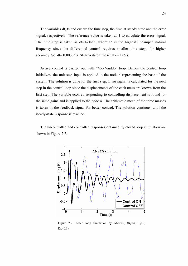
The variables dt, ts and err are the time step, the time at steady state and the error
signal, respectively. The reference value is taken as 1 to calculate the error signal.
The time step is taken as dt=1/60/f3, where f3 is the highest undamped natural
frequency since the differential control requires smaller time steps for higher
accuracy. So, dt= 0.00335 s. Steady-state time is taken as 5 s.
Active control is carried out with “*do-*enddo” loop. Before the control loop
initializes, the unit step input is applied to the node 4 representing the base of the
system. The solution is done for the first step. Error signal is calculated for the next
step in the control loop since the displacements of the each mass are known from the
first step. The variable ucon corresponding to controlling displacement is found for
the same gains and is applied to the node 4. The arithmetic mean of the three masses
is taken in the feedback signal for better control. The solution continues until the
steady-state response is reached.
The uncontrolled and controlled responses obtained by closed loop simulation are
shown in Figure 2.7.
Figure 2.7 Closed loop simulation by ANSYS, (Kp=4, KI=1,
KD=0.1).
25
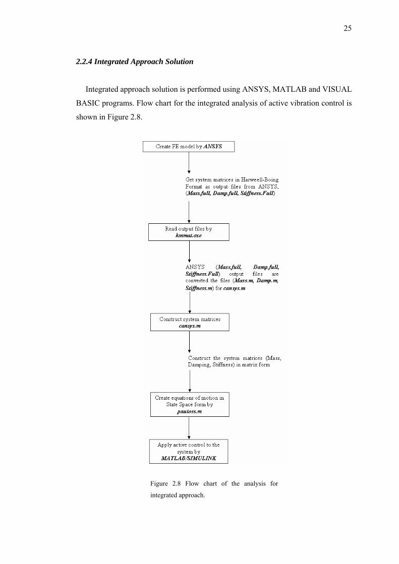
2.2.4 Integrated Approach Solution
Integrated approach solution is performed using ANSYS, MATLAB and VISUAL
BASIC programs. Flow chart for the integrated analysis of active vibration control is
shown in Figure 2.8.
Figure 2.8 Flow chart of the analysis for
integrated approach.
26
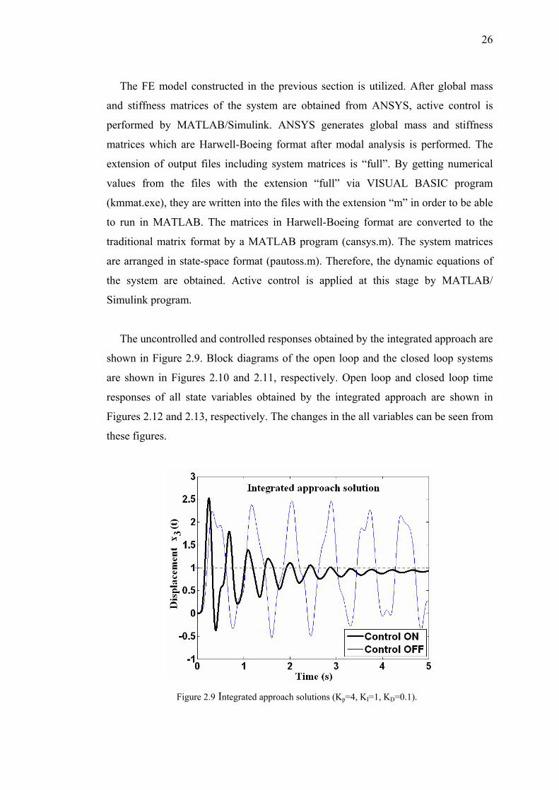
The FE model constructed in the previous section is utilized. After global mass
and stiffness matrices of the system are obtained from ANSYS, active control is
performed by MATLAB/Simulink. ANSYS generates global mass and stiffness
matrices which are Harwell-Boeing format after modal analysis is performed. The
extension of output files including system matrices is “full”. By getting numerical
values from the files with the extension “full” via VISUAL BASIC program
(kmmat.exe), they are written into the files with the extension “m” in order to be able
to run in MATLAB. The matrices in Harwell-Boeing format are converted to the
traditional matrix format by a MATLAB program (cansys.m). The system matrices
are arranged in state-space format (pautoss.m). Therefore, the dynamic equations of
the system are obtained. Active control is applied at this stage by MATLAB/
Simulink program.
The uncontrolled and controlled responses obtained by the integrated approach are
shown in Figure 2.9. Block diagrams of the open loop and the closed loop systems
are shown in Figures 2.10 and 2.11, respectively. Open loop and closed loop time
responses of all state variables obtained by the integrated approach are shown in
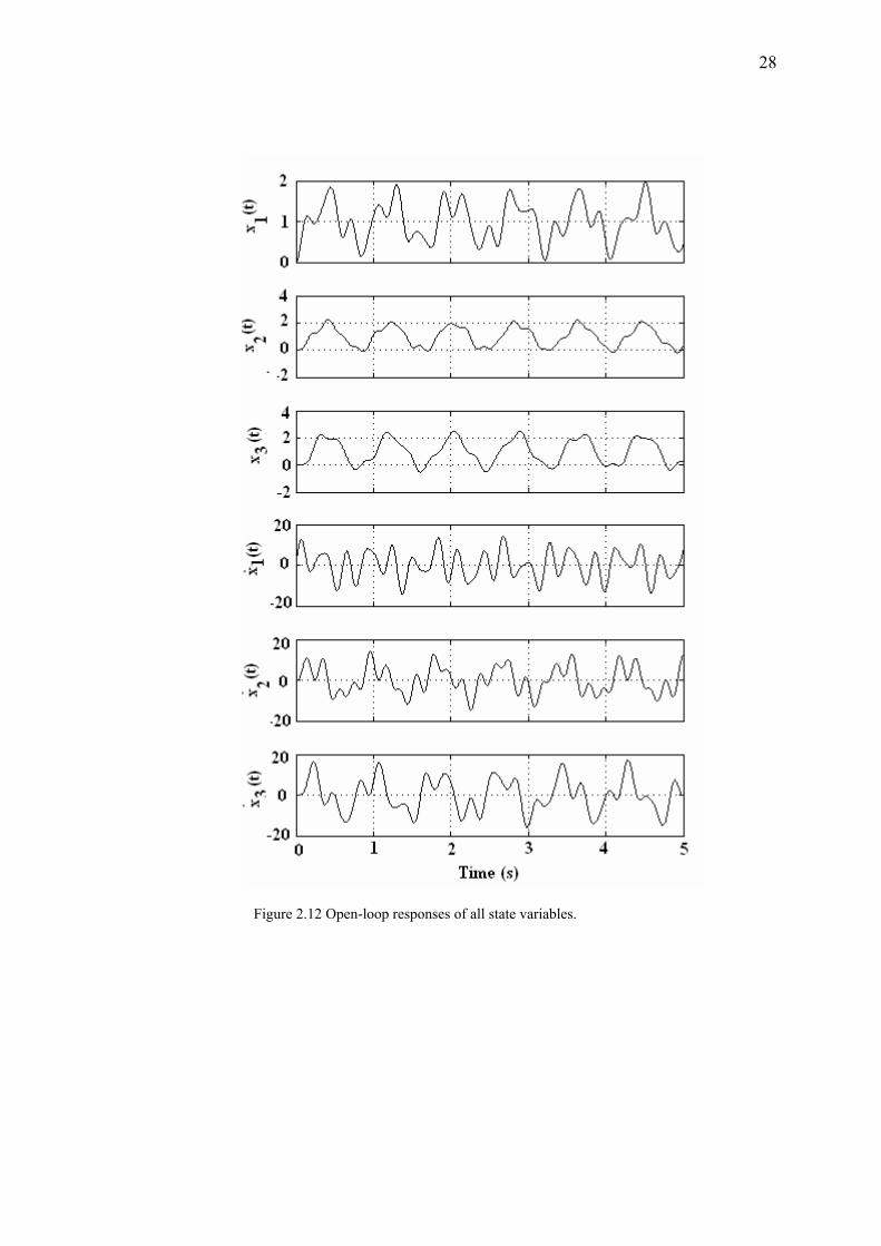
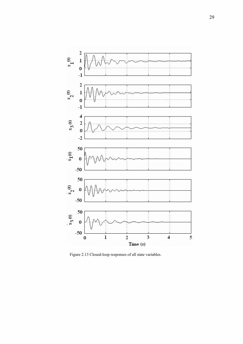
Figures 2.12 and 2.13, respectively. The changes in the all variables can be seen from
these figures.
Figure 2.9 Integrated approach solutions (Kp=4, KI=1, KD=0.1).
27
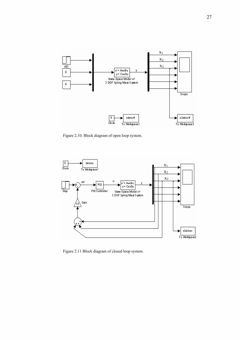
Figure 2.10. Block diagram of open loop system.
Figure 2.11 Block diagram of closed loop system.
x1
x2
x3
x1
x2
x3
28
Figure 2.12 Open-loop responses of all state variables.
29
Figure 2.13 Closed-loop responses of all state variables.
30
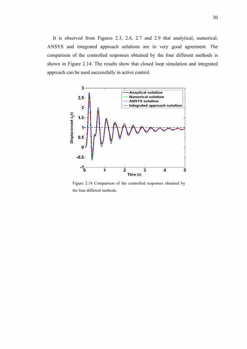
It is observed from Figures 2.3, 2.6, 2.7 and 2.9 that analytical, numerical,
ANSYS and integrated approach solutions are in very good agreement. The
comparison of the controlled responses obtained by the four different methods is
shown in Figure 2.14. The results show that closed loop simulation and integrated
approach can be used successfully in active control.
Figure 2.14 Comparison of the controlled responses obtained by
the four different methods.
31
CHAPTER THREE
ANALYSIS OF ACTIVE VIBRATION CONTROL
IN SMART STRUCTURES BY ANSYS
3.1 Introduction
It is possible to model smart structures with piezoelectric materials by ANSYS/
Multiphysics product. In this chapter, the integration of control actions to the ANSYS
solution is realized. First, the procedure is tested on the active vibration control problem
with two-degrees of freedom system. The analytical results obtained by the Laplace
transform method, and by ANSYS are compared. Then, the smart structures are studied
by ANSYS. The input reference value is taken as zero in the closed loop vibration
control. The instantaneous value of the strain at the sensor location at a time step is
subtracted from zero to find the error signal value. The error value is multiplied by the
control gain to calculate the voltage value which is used as the input to the actuator
nodes. The process is continued with the selected time step until the steady-state value
is approximately reached. The results are obtained for the structures analyzed in other
studies. Also, the active vibration control of a circular disc and a square plate is studied.
3.2 A Two-Degrees of Freedom System
3.2.1 Analytical Solution
The system and the block diagram of the closed loop control system are shown in
Figure 3.1. f2 is the vibration generating force, and f1 is the controlling force. Xr, X2, F1,
and F2 are the Laplace transforms of the reference input (xr), output displacement (x2),
the forces f1, and f2, respectively. G1 is the transfer function of the control action, and it
is taken as
(3.1) sKs
KK)s(G D
IP1 ++=
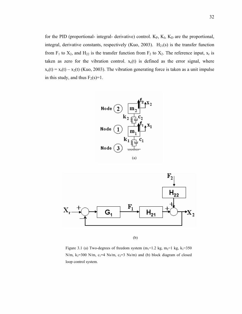
32
for the PID (proportional- integral- derivative) control. KP, KI, KD are the proportional,
integral, derivative constants, respectively (Kuo, 2003). H21(s) is the transfer function
from F1 to X2, and H22 is the transfer function from F2 to X2. The reference input, xr is
taken as zero for the vibration control. xe(t) is defined as the error signal, where
xe(t) = xr(t) – x2(t) (Kuo, 2003). The vibration generating force is taken as a unit impulse
in this study, and thus F2(s)=1.
(a)
(b)
Figure 3.1 (a) Two-degrees of freedom system (m1=1.2 kg, m2=1 kg, k1=350
N/m, k2=300 N/m, c1=4 Ns/m, c2=3 Ns/m) and (b) block diagram of closed
loop control system.
33
Applying the Lagrange’s equation (Williams, 1996), the mathematical model of the
system in Figure 3.1 (a) can be found as:
⎭⎬⎫
⎩⎨⎧
=⎭⎬⎫
⎩⎨⎧⎥⎦
⎤⎢⎣
⎡−
−++
⎭⎬⎫
⎩⎨⎧⎥⎦
⎤⎢⎣
⎡−
−++
⎭⎬⎫
⎩⎨⎧⎥⎦
⎤⎢⎣
⎡
2
1
2
1
22
221
2
1
22
221
2
1
2
1
ff
xx
kkkkk
xx
ccccc
xx
m00m
&
&
&&
&& (3.2)
Then, the transfer functions can be written as the following, after substituting the
values of the masses, damping and spring constants.
)s(D)100s(3)s(H21
+= (3.3)
)s(D)650s7s2.1()s(H
2
22++
= (3.4)
where
105000s2250s1022s6.10s2.1)s(D 234 ++++= (3.5)
Substituting Xr(s)=0 and F2(s)=1, the transfer function of the closed loop system in
Figure 3.1 (b) is found as
(3.6)
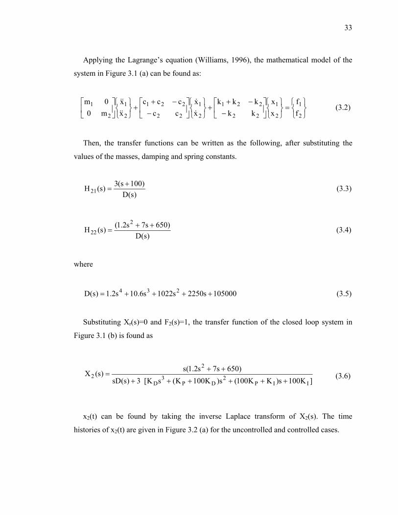
x2(t) can be found by taking the inverse Laplace transform of X2(s). The time
histories of x2(t) are given in Figure 3.2 (a) for the uncontrolled and controlled cases.
]K100s)KK100(s)K100K(sK[3)s(sD)650s7s2.1(s)s(X
IIP2
DP3
D
2
2++++++
++=
34
0 0.5 1 1.5 2 2.5-0.06
-0.04
-0.02
0
0.02
0.04
0.06
Time (s)
X 2 (m)
Control OffControl On
ANSYS Solution
0 0.5 1 1.5 2 2.5-0.06
-0.04
-0.02
0
0.02
0.04
0.06
Time (s)
X 2 (m)
Control OffControl On
Analytical Solution
(a)
(b)
Figure 3.2 (a) Analytical and (b) ANSYS solutions. (KP=100, KI=40,
and KD=10 for Control On).
35
3.2.2 Closed Loop Simulation by ANSYS
For the solution by ANSYS, MASS21 and COMBIN14 elements are used. The
system in Figure 3.1 (a) is modeled. Modal analysis is performed and two undamped
natural frequencies are found. The time step (Δt) can be taken as 1/(20fh), where fh is
the highest frequency. However, it is taken as 1/(60fh) because the differential control
action requires smaller time steps for higher accuracy. ts is the time at which the steady-
state response is approximately reached. The undamped natural frequencies for the
open-loop system are found as 1.75 and 4.27 Hz. Therefore, Δt = 0.0039 s.
The value of f2 is 1/Δt at t=Δt, and it is zero otherwise. The value of f1 is zero at t=Δt.
The part of the macro which enables the calculations for the closed loop analysis for
t>Δt is given below:
sum=0
errp=0
*do,t,2*dt,ts,dt
*get,e1,node,2,u,x
err=0-e1
sum=sum+err*dt
dif=(err-errp)/dt
f1=kp*err+ki*sum+kd*dif
f,1,fx,f1
errp=err
time,t
solve
*enddo
36
The variables dt, ts, kp, ki, and kd are defined in the previous part of the macro, and
they correspond to ∆t, ts, KP, KI, and KD, respectively. The variable f1 corresponds to the
actuation force f1.
The time histories of x2(t) obtained by the ANSYS solution are given in Figure 3.2
(b) for the uncontrolled and controlled cases. It is observed form Figure 3.2 (a) and 3.2
(b) that the analytical and ANSYS solutions are in agreement.
After testing the success of the ANSYS solution by comparing it with the analytical
solution for the two-degrees of system, the ANSYS solution is used for the smart
structures below.
3.3 Active Vibration Control in Smart Structures
In this section, the active vibration control in smart structures is simulated by
ANSYS. The block diagram of the analysis is show in Figure 3.3.
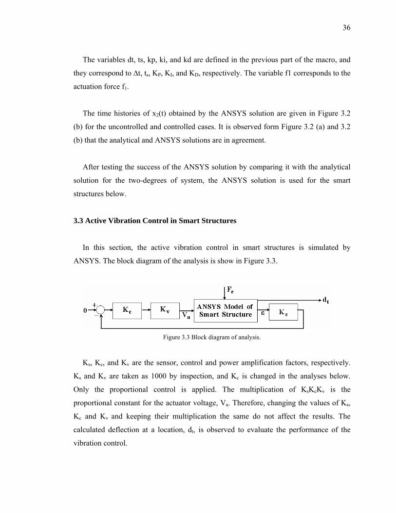
Figure 3.3 Block diagram of analysis.
Ks, Kc, and Kv are the sensor, control and power amplification factors, respectively.
Ks and Kv are taken as 1000 by inspection, and Kc is changed in the analyses below.
Only the proportional control is applied. The multiplication of KsKcKv is the
proportional constant for the actuator voltage, Va. Therefore, changing the values of Ks,
Kc and Kv and keeping their multiplication the same do not affect the results. The
calculated deflection at a location, dt, is observed to evaluate the performance of the
vibration control.
37
3.3.1 Beam Type Structures
First, beam type structures are considered. The configuration of the structure is shown
in Figure 3.4.
Figure 3.4 Configuration for beam type structure.
The strain value at the sensor location is taken as the feedback. The dimensions and
the distances for the cases studied are given in Table 3.1. This type of structure has been
studied by many researchers (Manning et al., 2000, Gaudenzi, et al., 2000, Bruant et al.,
2001, Singh et al., 2003, Xu & Koko, 2004). The corresponding reference where the
same structure was studied as indicated in Table 3.1.
Table 3.1 Dimensions and distances for the cases.
Case Reference
numbers
Dimensions of
structurea
(mm)
Dimensions of
actuatorb
(mm)
da : Actuator
distance
(mm)
ds: Sensor
distance
(mm)
1 1 504x25.4x0.8 72x25.4x0.61 12 48
2 1 224.25x25x0.965 39x25x0.75 9.8 29.3
3 2 160x25.4x2 46x20.6x0.254 5.7 28.5
4 3 348x24x1 72x24x0.5 12 48 a Aluminum, b PZT-5H 1 Xu & Koko, 2004, 2 Gaudenzi, et al., 2000, 3 Manning et al., 2000
38
A macro is written using APDL. The macro starts with the definition of the variables
for the dimensions of the structure. Then the three dimensional material properties are
assigned. The part of the macro where the material properties are assigned is given
below. Material 1 is the metal, and Material 2 (PZT-5H) is the actuator material.
mp,ex,1,68e9 ! Elasticity modulus for metal
mp,dens,1,2800 ! Density
mp,nuxy,1,0.32 ! Poisson's ratio
mp,dens,2,7500 ! Density for piez. material
mp,perx,2,15.03E-9 ! Permittivity in x direction
mp,pery,2,15.03E-9 ! Permittivity in y direction
mp,perz,2,13E-9 ! Permittivity in z direction
tb,piez,2 ! Define piez. table
tbdata,16,17 ! E16 piezoelectric constant
tbdata,14,17 ! E25
tbdata,3,-6.5 ! E31
tbdata,6,-6.5 ! E32
tbdata,9,23.3 ! E33
tb,anel,2 ! Define structural table
tbdata,1,126E9,79.5E9,84.1E9 ! C11,C12,C13
tbdata,7,126E9,84.1E9 ! C22,C23
tbdata,12,117E9 ! C33
tbdata,16,23.3E9 ! C44
tbdata,19,23E9 ! C55
tbdata,21,23E9 ! C66
The macro is continued to create nodes and finite elements. SOLID45 elements are
used for the metal part, and SOLID5 elements are used for the piezoelectric part of the
structure. The FE model for Case 1 is shown in Figure 3.5.
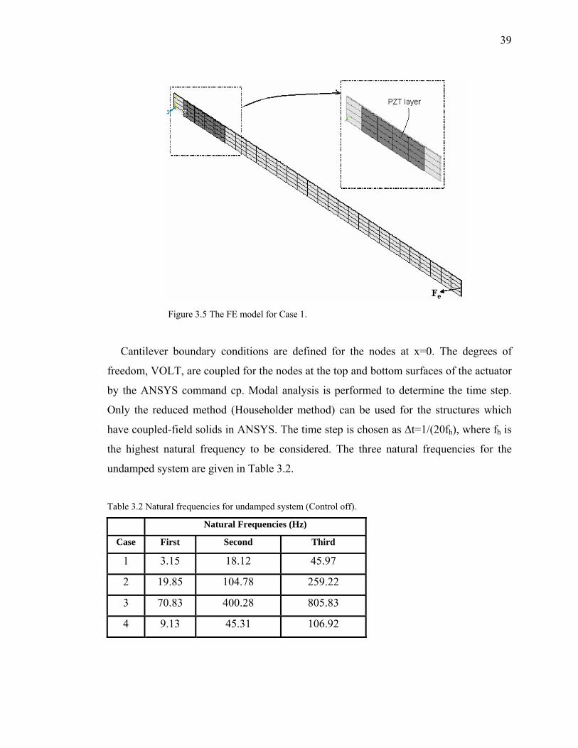
39
Figure 3.5 The FE model for Case 1.
Cantilever boundary conditions are defined for the nodes at x=0. The degrees of
freedom, VOLT, are coupled for the nodes at the top and bottom surfaces of the actuator
by the ANSYS command cp. Modal analysis is performed to determine the time step.
Only the reduced method (Householder method) can be used for the structures which
have coupled-field solids in ANSYS. The time step is chosen as ∆t=1/(20fh), where fh is
the highest natural frequency to be considered. The three natural frequencies for the
undamped system are given in Table 3.2.
Table 3.2 Natural frequencies for undamped system (Control off).
Natural Frequencies (Hz)
Case First Second Third
1 3.15 18.12 45.97
2 19.85 104.78 259.22
3 70.83 400.28 805.83
4 9.13 45.31 106.92
40
The first mode is considered to calculate the time step and Δt is 0.0159, 0.0025,
0.0007, and 0.0055 for Case 1, 2, 3, and 4, respectively.
In the transient analysis, the coefficients of Rayleigh damping (α and β) are defined.
α=β is taken in this study. Fe=F0 for t=Δt and Fe=0 at the subsequent time steps. Va=0 at
t=Δt. The strain is calculated at the selected sensor location and it is multiplied by Ks,
and then it is subtracted from zero. The zero value is the reference input value to control
the vibration. The difference between the input reference and the sensor signal is called
the error signal (Kuo, 2003). The error value is multiplied by Kc and Kv to determine Va
at a time step.
The part of the macro which enables the calculations for the closed loop analysis for
t>Δt is given below.
*do,t,2*dt,ts,dt
*get,u1,node,nr,u,x
*get,u2,node,nr1,u,x
err=0-ks*(u2-u1)/dx
va=kc*kv*err
d,nv,volt,va
time,t
solve
*enddo
The variables ks, kc, and kv correspond to Ks, Kc, and Kv, respectively. nr and nr1 are
the node numbers used to calculate the strain. These nodes are adjacent in the x
direction, and dx is the distance between them.
41
The values of Rayleigh damping coefficients, α and β; the impulsive force, F0; and
the control gain, Kc, are taken differently for each case. The values of F0 and Kc are
limited by the maximum value of the actuator voltage which can be applied to the
actuator safely without breaking it. The maximum voltage per thickness of the
piezoelectric material is taken as 235 V/mm. Therefore, the actuator voltages are kept
below 143.4, 176.3, 59.7, and 117.5 V for Case 1, 2, 3, and 4, respectively.
The tip deflections and actuator voltages for different values of the control gain for
Case 1 are shown in Figure 3.6. It is observed that as Kc increases the vibration settling
time decreases and the actuator voltage increases. The case, Kc=5, cannot be applied
because the absolute value of the actuator voltage exceeds the limit value of 143.4 V.
The tip displacement and the actuator voltages for Case 3 and 4 are shown in Figure
3.7 and 3.8. Similar results are obtained in the references given in Table 3.1. Different
control strategies are applied in the references and some of the results are verified by
experiments (Gaudenzi, et al., 2000, Manning et al., 2000, Xu & Koko, 2004).
42
0 0.5 1 1.5-0.015
-0.01
-0.005
0
0.005
0.01
0.015
Time (s)
Tip
Def
lect
ion
(m)
Kc=2 Kc=5Kc=0 Kc=3.3
Case 1
1 2 3 4
1
2
3
4
0 0.5 1 1.5-300
-200
-100
0
100
200
Time (s)
Act
uato
r Vol
tage
(V)
Kc=0 Kc=2 Kc=3.3 Kc=5
Case 1
4 321
1 2
3
4
(a)
(b)
Figure 3.6 (a) Tip deflections and (b) actuator voltages for different values
of control gain. (F0=0.1, α=0.001).
43
0 0.1 0.2 0.3 0.4 0.5-200
-150
-100
-50
0
50
100
Time (s)
Act
uato
r Vol
tage
(V)
Kc=0Kc=5
Case 2
0 0.1 0.2 0.3 0.4 0.5-1.5
-1
-0.5
0
0.5
1
1.5 x 10⁻³
Time (s)
Tip
Def
lect
ion
(m)
Kc=0Kc=5
Case 2
(a)
(b)
Figure 3.7 (a) Tip deflections and (b) actuator voltages for Case 2.
(F0=0.2, α=0.0003 ).
44
0 0.02 0.04 0.06 0.08 0.1 0.12 0.14-6
-4
-2
0
2
4
6 x 10⁻⁴
Time (s)
Tip
Def
lect
ion
(m)
Kc=0Kc=1
Case 3
0 0.2 0.4 0.6 0.8 1-4
-3
-2
-1
0
1
2
3
4 x 10⁻³
Time (s)
Tip
Def
lect
ion
(m)
Kc=0Kc=4
Case 4
(a)
(b)
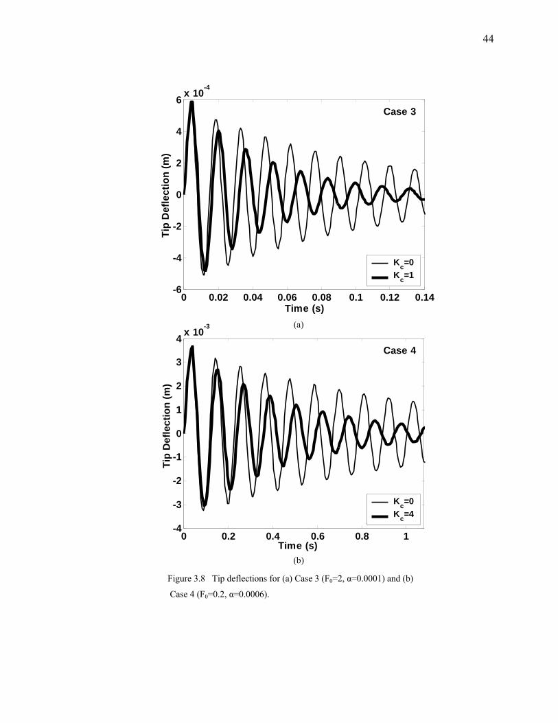
Figure 3.8 Tip deflections for (a) Case 3 (F0=2, α=0.0001) and (b)
Case 4 (F0=0.2, α=0.0006).
45
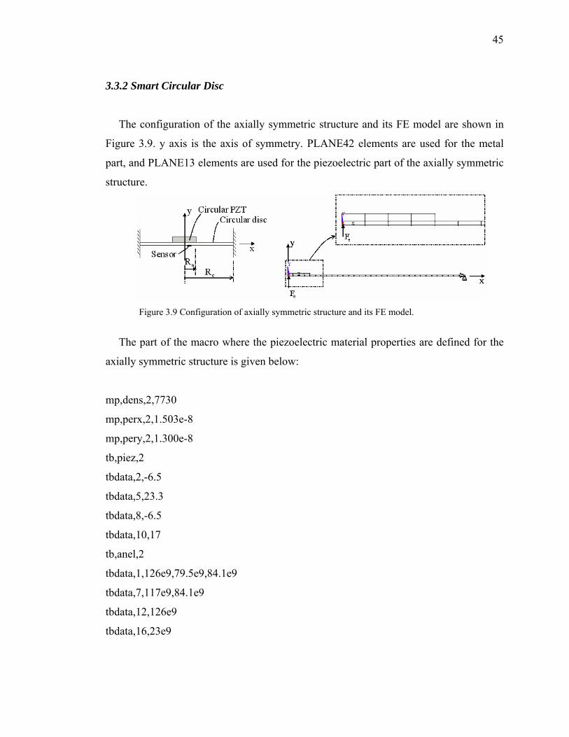
3.3.2 Smart Circular Disc
The configuration of the axially symmetric structure and its FE model are shown in
Figure 3.9. y axis is the axis of symmetry. PLANE42 elements are used for the metal
part, and PLANE13 elements are used for the piezoelectric part of the axially symmetric
structure.
Figure 3.9 Configuration of axially symmetric structure and its FE model.
The part of the macro where the piezoelectric material properties are defined for the
axially symmetric structure is given below:
mp,dens,2,7730
mp,perx,2,1.503e-8
mp,pery,2,1.300e-8
tb,piez,2
tbdata,2,-6.5
tbdata,5,23.3
tbdata,8,-6.5
tbdata,10,17
tb,anel,2
tbdata,1,126e9,79.5e9,84.1e9
tbdata,7,117e9,84.1e9
tbdata,12,126e9
tbdata,16,23e9
46
0 0.02 0.04 0.06 0.08 0.1-4
-2
0
2
4
6 x 10⁻⁵
Time (s)
Cen
ter D
efle
ctio
n (m
)
Kc=0Kc=25
Case 6 (Ra/Rc=3/16)
0 0.02 0.04 0.06 0.08 0.1-6
-4
-2
0
2
4
6 x 10⁻⁵
Time (s)
Cen
ter D
efle
ctio
n (m
)
Kc=0Kc=15
Case 5 (Ra/Rc=2/16)
(a)
(b)
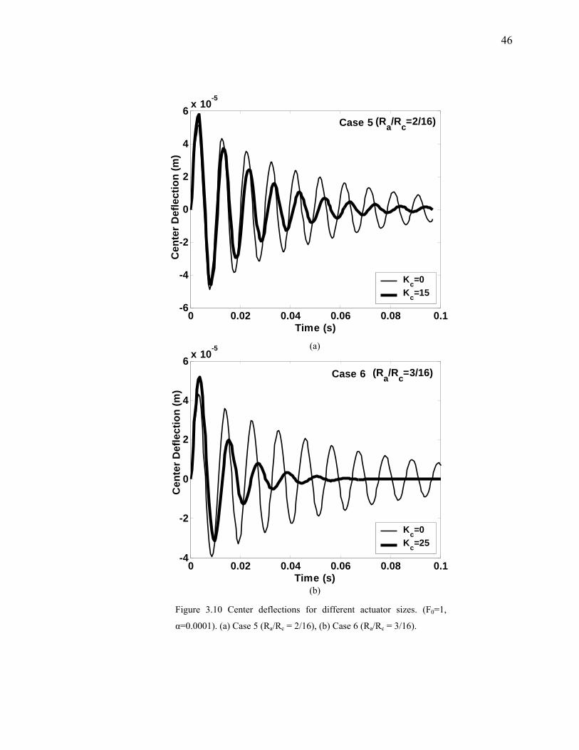
Figure 3.10 Center deflections for different actuator sizes. (F0=1,
α=0.0001). (a) Case 5 (Ra/Rc = 2/16), (b) Case 6 (Ra/Rc = 3/16).
47
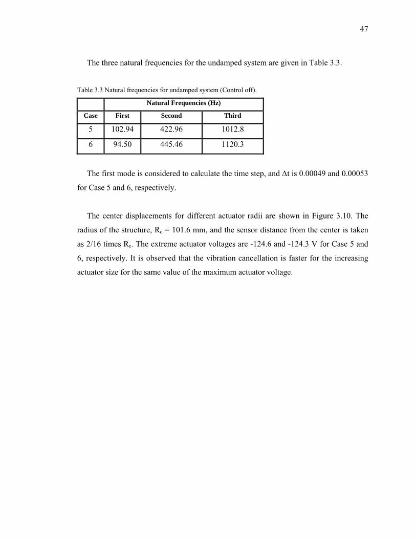
The three natural frequencies for the undamped system are given in Table 3.3.
Table 3.3 Natural frequencies for undamped system (Control off).
Natural Frequencies (Hz)
Case First Second Third
5 102.94 422.96 1012.8
6 94.50 445.46 1120.3
The first mode is considered to calculate the time step, and Δt is 0.00049 and 0.00053
for Case 5 and 6, respectively.
The center displacements for different actuator radii are shown in Figure 3.10. The
radius of the structure, Rc = 101.6 mm, and the sensor distance from the center is taken
as 2/16 times Rc. The extreme actuator voltages are -124.6 and -124.3 V for Case 5 and
6, respectively. It is observed that the vibration cancellation is faster for the increasing
actuator size for the same value of the maximum actuator voltage.
48
3.3.3 Smart Plate
Lim (2003) modeled a plate structure with integrated piezoelectric patches using the
FE method which is based on the combination of three-dimensional piezoelectric, flat
shell and transition elements. For closed loop control, constant velocity feedback and
constant displacement feedback control algorithms are used to suppress the dynamic
response of the smart plate. By using strategically located sensor/actuator pairs, several
modes of clamped plate are successfully controlled. It is reported that discrete
sensor/actuator piezoelectric patches should be preferred over distributed piezoelectric
films due to the lower weight, effective control authority and modest values of actuator
voltages.
Effective sensing and control depend on the locations of sensors and actuators. The
actuator locations are very important in order to maximize actuator effectiveness. The
positions of the plate at which the mechanical strain is highest are the best locations for
sensors and actuators. The objective of the multimode control is to place all of the
actuators in regions of high average strain and away from areas of zero strain (nodal
line). Modal analysis of the plate is required to design the locations of sensors and
actuators.
The smart plate studied by Lim (2003) is considered for the closed loop simulations
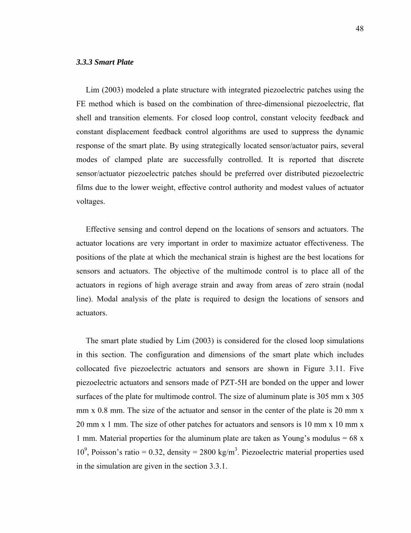
in this section. The configuration and dimensions of the smart plate which includes
collocated five piezoelectric actuators and sensors are shown in Figure 3.11. Five
piezoelectric actuators and sensors made of PZT-5H are bonded on the upper and lower
surfaces of the plate for multimode control. The size of aluminum plate is 305 mm x 305
mm x 0.8 mm. The size of the actuator and sensor in the center of the plate is 20 mm x
20 mm x 1 mm. The size of other patches for actuators and sensors is 10 mm x 10 mm x
1 mm. Material properties for the aluminum plate are taken as Young’s modulus = 68 x
109, Poisson’s ratio = 0.32, density = 2800 kg/m3. Piezoelectric material properties used
in the simulation are given in the section 3.3.1.
49
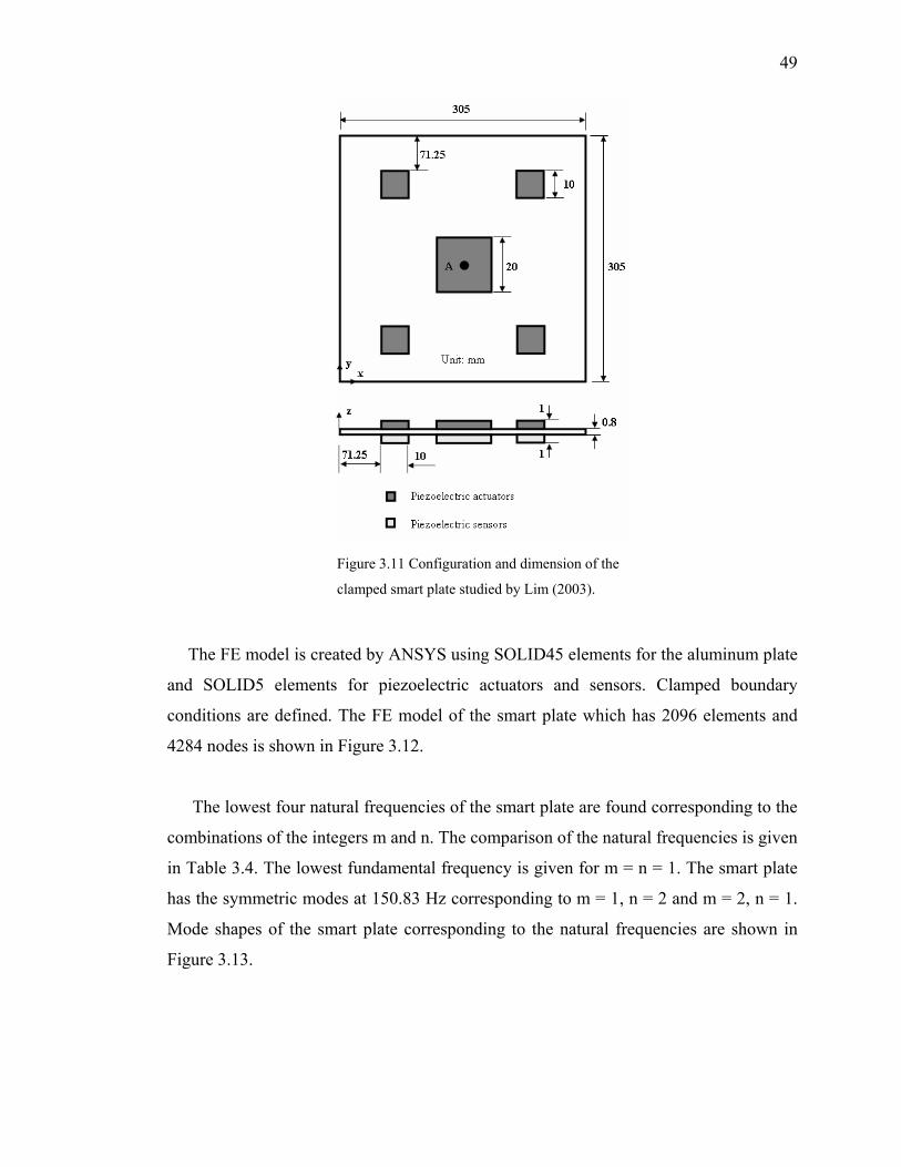
The FE model is created by ANSYS using SOLID45 elements for the aluminum plate
and SOLID5 elements for piezoelectric actuators and sensors. Clamped boundary
conditions are defined. The FE model of the smart plate which has 2096 elements and
4284 nodes is shown in Figure 3.12.
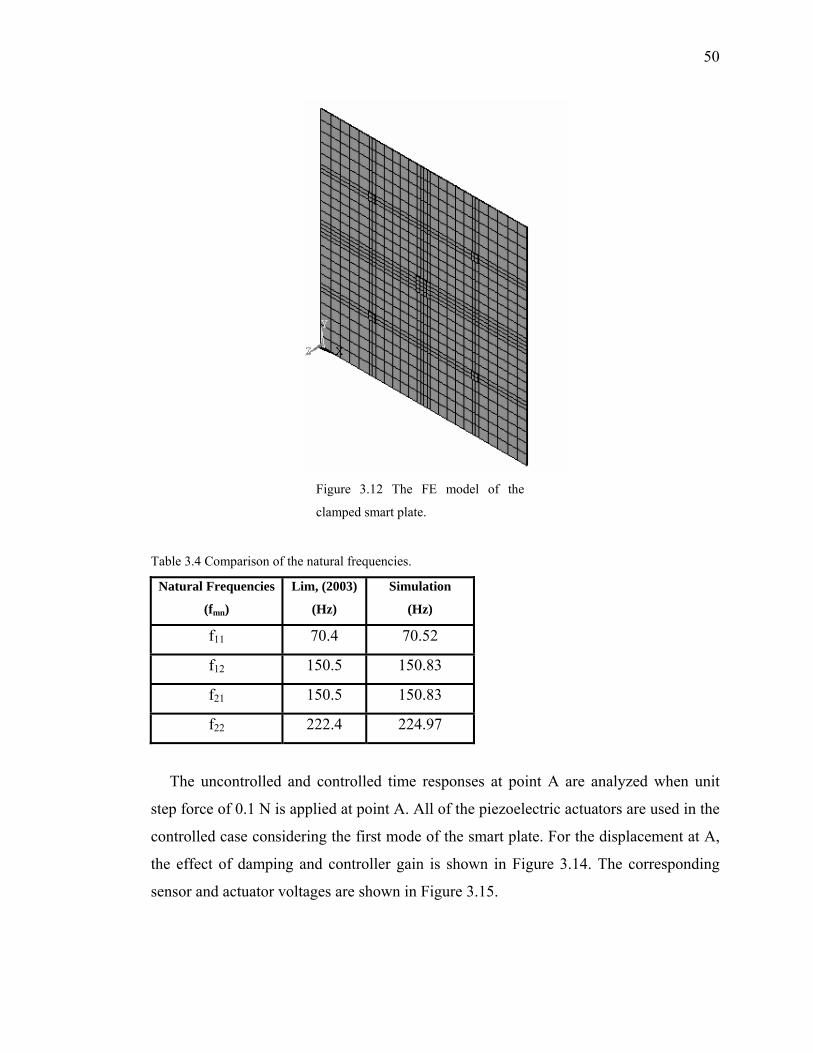
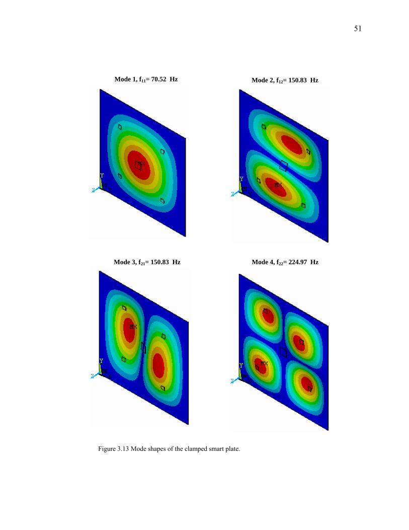
The lowest four natural frequencies of the smart plate are found corresponding to the
combinations of the integers m and n. The comparison of the natural frequencies is given
in Table 3.4. The lowest fundamental frequency is given for m = n = 1. The smart plate
has the symmetric modes at 150.83 Hz corresponding to m = 1, n = 2 and m = 2, n = 1.
Mode shapes of the smart plate corresponding to the natural frequencies are shown in
Figure 3.13.
Figure 3.11 Configuration and dimension of the
clamped smart plate studied by Lim (2003).
50
Table 3.4 Comparison of the natural frequencies.
Natural Frequencies
(fmn)
Lim, (2003)
(Hz)
Simulation
(Hz)
f11 70.4 70.52
f12 150.5 150.83
f21 150.5 150.83
f22 222.4 224.97
The uncontrolled and controlled time responses at point A are analyzed when unit
step force of 0.1 N is applied at point A. All of the piezoelectric actuators are used in the
controlled case considering the first mode of the smart plate. For the displacement at A,
the effect of damping and controller gain is shown in Figure 3.14. The corresponding
sensor and actuator voltages are shown in Figure 3.15.
Figure 3.12 The FE model of the
clamped smart plate.
51
Figure 3.13 Mode shapes of the clamped smart plate.
Mode 1, f11= 70.52 Hz Mode 2, f12= 150.83 Hz
Mode 3, f21= 150.83 Hz Mode 4, f22= 224.97 Hz
52
(a)
(b)
Figure 3.14 Center deflections at point A for (a) Case 7 (F0=-0.1,
α=0.000005 β= α) and (b) Case 8 (F0=-0.1, α=0.00001 β= α).
53
(a)
(b)
Figure 3.15 (a) Actuation voltages of the center actuator for Case
7 and Case 8 and (b) Sensor voltages of the center sensor for
Case 7 and Case 8.
54
3.4 Characteristics of Vibration Signals
The vibration signals given in Figures 3.6, 3.7, 3.8, 3.10 and 3.14 can be
approximately modeled by the signal d(t)= ),tsin(Ae tn ωξω− where 2n 1 ξ−ω=ω . A
is the amplitude, ξ is the damping ratio, nω is the undamped frequency, ω is the
damped frequency. The maximum and minimum values of the actuator voltages (Vmax
and Vmin), and the values of ξ and fd are listed for different cases in Table 3.4, where
fd= )2/( πω . It is observed from Table 3.5 that the closed loop control increases the
damping ratio and decreases the damped frequency.
Table 3.5 Characteristics of vibration signals.
Control Off Control On Cases
ξ fd (Hz) Kc ξ fd (Hz) Vmax (V) Vmin (V)
1 0.011 3.11 3.3 0.061 2.83 115.4 -139.0
2 0.019 19.61 5 0.153 16.54 97.2 -155.0
3 0.023 69.10 1 0.056 62.96 49.7 -58.1
4 0.017 9.13 4 0.044 8.59 82.7 -91.8
6 0.029 93.34 25 0.145 85.91 124.3 -69.9
7 0.0035 70.523 10 0.012 70.518 -5.54 5.80
8 0.0050 70.522 15 0.025 70.501 -11.00 10.26
55
CHAPTER FOUR
EXPERIMENTAL ANALYSIS OF ACTIVE VIBRATION CONTROL
IN SMART STRUCTURES AND COMPARISON WITH
CLOSED LOOP-FINITE ELEMENT SIMULATIONS
4.1 Introduction
The closed loop control law can be incorporated into the FE models by using
APDL. The control gains and vibration controlling piezoelectric actuation voltages
can be determined by the simulations. In this study, the experiments are conducted to
verify these simulation results. A cantilever aluminum beam with piezoelectric
(Lead-Zirconate-Titanate) actuator and strain gage sensor is considered. First, modal
analysis is done. A chirp signal for the first two modes is applied to the piezoelectric
actuator as the input. The natural frequencies are observed in the frequency domain.
Then, free vibration of the beam under an initial tip displacement is considered.
Control OFF and Control ON vibration signals are obtained for various gains. In
addition to strain feedback in active control of the beam, displacement feedback is
also examined. The signals for all cases are found experimentally and also by the
simulation. The experimental results are obtained by using LabVIEW program. It is
observed that the simulation results obtained by the integrated control and the FE
procedure are in good agreement with the experimental results.
4.2 Experimental System
A smart beam is produced as a test specimen to be used in the experiments for the
comparison with simulation results. The smart beam consists of an aluminum beam,
a piezoelectric patch as an actuator, and a strain gage as a sensor. The piezoelectric
actuator BM532 of SENSORTECH is bonded onto beam using ELECOLIT 325
conductive epoxy. A wire is soldered on the piezoelectric actuator with S-Sn60/Pb40
solder.

56
The soldering process should be as short as possible to avoid hazarding the
piezoelectric patch. TML FRA-3-11-1L type strain gage of 120 ohm is glued onto
the lower surface of the beam in the x direction.
The configuration of the smart beam which has cantilever boundary conditions is
parametrically shown in Figure 4.1 (a). The dimensions of the smart beam are given
in Table 4.1. The material properties of the smart beam are given in Table 4.2.
(a)
(b)
Figure 4.1 (a) Configuration of the cantilever smart beam,
(b) Cantilever test rig in the experiment.
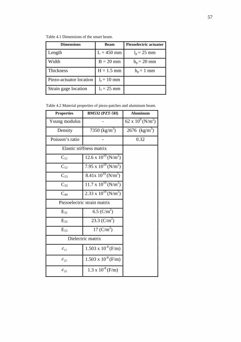
57
Table 4.1 Dimensions of the smart beam.
Dimensions Beam Piezoelectric actuator
Length L = 450 mm lp = 25 mm
Width B = 20 mm bp = 20 mm
Thickness H = 1.5 mm hp = 1 mm
Piezo-actuator location ls = 10 mm
Strain gage location l1 = 25 mm
Table 4.2 Material properties of piezo-patches and aluminum beam.
Properties BM532 (PZT-5H) Aluminum
Young modulus - 62 x 109 (N/m2)
Density 7350 (kg/m3) 2676 (kg/m3)
Poisson’s ratio - 0.32
Elastic stiffness matrix
C11 12.6 x 10¹⁰ (N/m2)
C12 7.95 x 10¹⁰ (N/m2)
C13 8.41x 10¹⁰ (N/m2)
C33 11.7 x 10¹⁰ (N/m2)
C44 2.33 x 10¹⁰ (N/m2)
Piezoelectric strain matrix
E31 6.5 (C/m2)
E33 23.3 (C/m2)
E15 17 (C/m2)
Dielectric matrix
11ε 1.503 x 10⁻⁸ (F/m)
22ε 1.503 x 10⁻⁸ (F/m)
33ε 1.3 x 10⁻⁸ (F/m)
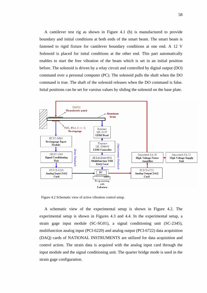
58
A cantilever test rig as shown in Figure 4.1 (b) is manufactured to provide
boundary and initial conditions at both ends of the smart beam. The smart beam is
fastened to rigid fixture for cantilever boundary conditions at one end. A 12 V
Solenoid is placed for inital conditions at the other end. This part automatically
enables to start the free vibration of the beam which is set in an initial position
before. The solenoid is driven by a relay circuit and controlled by digital output (DO)
command over a personal computer (PC). The solenoid pulls the shaft when the DO
command is true. The shaft of the solenoid releases when the DO command is false.
Inital positions can be set for varoius values by sliding the solenoid on the base plate.
Figure 4.2 Schematic view of active vibration control setup.
A schematic view of the experimental setup is shown in Figure 4.2. The
experimental setup is shown in Figures 4.3 and 4.4. In the experimental setup, a
strain gage input module (SC-SG01), a signal conditioning unit (SC-2345),
multifunction analog input (PCI-6220) and analog output (PCI-6722) data acquisition
(DAQ) cards of NATIONAL INSTRUMENTS are utilized for data acquisition and
control action. The strain data is acquired with the analog input card through the
input module and the signal conditioning unit. The quarter bridge mode is used in the
strain gage configuration.
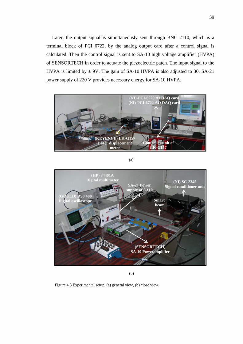
59
Later, the output signal is simultaneously sent through BNC 2110, which is a
terminal block of PCI 6722, by the analog output card after a control signal is
calculated. Then the control signal is sent to SA-10 high voltage amplifier (HVPA)
of SENSORTECH in order to actuate the piezoelectric patch. The input signal to the
HVPA is limited by ± 9V. The gain of SA-10 HVPA is also adjusted to 30. SA-21
power supply of 220 V provides necessary energy for SA-10 HVPA.
Smart beam
(SENSORTECH) SA-10 Poweramplifier
(HP) 34401A Digital multimeter
(GOULD) DS0 400 Digital oscilloscope
(NI) SC-2345 Signal conditioner unit SA-21 Power
supply of SA10
(NI)-PCI-6220 AI DAQ card (NI)-PCI-6722 AO DAQ card
Controller unit of LK-G157
(KEYENCE) LK-G157 Laser displacement
meter
Figure 4.3 Experimental setup, (a) general view, (b) close view.
(a)
(b)
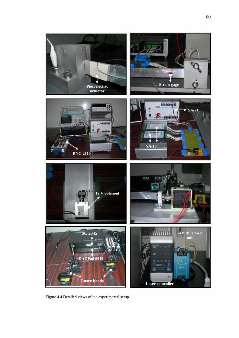
60
Figure 4.4 Detailed views of the experimental setup.
12 V Solenoid
SC 2345
DAQPad 6015
Laser headsLaser controller
24V DC Power unit
Piezoelectric actuator
Strain gage
SA-21
SA-10
BNC-2110
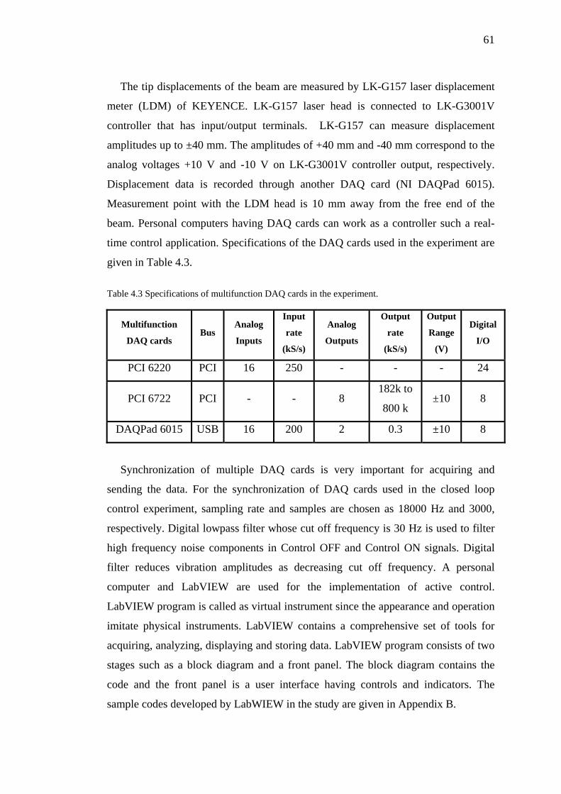
61
The tip displacements of the beam are measured by LK-G157 laser displacement
meter (LDM) of KEYENCE. LK-G157 laser head is connected to LK-G3001V
controller that has input/output terminals. LK-G157 can measure displacement
amplitudes up to ±40 mm. The amplitudes of +40 mm and -40 mm correspond to the
analog voltages +10 V and -10 V on LK-G3001V controller output, respectively.
Displacement data is recorded through another DAQ card (NI DAQPad 6015).
Measurement point with the LDM head is 10 mm away from the free end of the
beam. Personal computers having DAQ cards can work as a controller such a real-
time control application. Specifications of the DAQ cards used in the experiment are
given in Table 4.3.
Table 4.3 Specifications of multifunction DAQ cards in the experiment.
Synchronization of multiple DAQ cards is very important for acquiring and
sending the data. For the synchronization of DAQ cards used in the closed loop
control experiment, sampling rate and samples are chosen as 18000 Hz and 3000,
respectively. Digital lowpass filter whose cut off frequency is 30 Hz is used to filter
high frequency noise components in Control OFF and Control ON signals. Digital
filter reduces vibration amplitudes as decreasing cut off frequency. A personal
computer and LabVIEW are used for the implementation of active control.
LabVIEW program is called as virtual instrument since the appearance and operation
imitate physical instruments. LabVIEW contains a comprehensive set of tools for
acquiring, analyzing, displaying and storing data. LabVIEW program consists of two
stages such as a block diagram and a front panel. The block diagram contains the
code and the front panel is a user interface having controls and indicators. The
sample codes developed by LabWIEW in the study are given in Appendix B.
Multifunction
DAQ cards Bus
Analog
Inputs
Input
rate
(kS/s)
Analog
Outputs
Output
rate
(kS/s)
Output
Range
(V)
Digital
I/O
PCI 6220 PCI 16 250 - - - 24
PCI 6722 PCI - - 8 182k to
800 k ±10 8
DAQPad 6015 USB 16 200 2 0.3 ±10 8
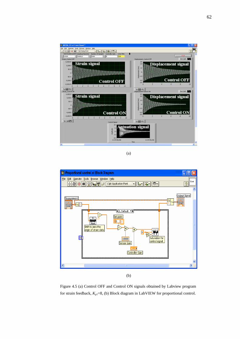
62
(a)
(b)
Figure 4.5 (a) Control OFF and Control ON signals obtained by Labview program
for strain feedback, Kp1=8, (b) Block diagram in LabVIEW for proportional control.
63
Data acquisition and control programs are developed by LabVIEW (version 7.0)
in the experiment. The active control program developed in LabVIEW consists of 7
sequences including digital output (DO), analog input (AI) and analog output (AO)
applications. 1, 3, 5 and 7 sequences control DO that enables the pushing and the
pulling of the solenoid shaft. Control OFF and Control ON signals of the smart beam
are obtained in the sequences 2 and 6. These signals obtained by LabVIEW program
are shown in Figure 4.5 (a). The sequence 4 is a waiting mode to pass Control ON
test. The experiment is repeated for various gain values.
Closed loop control in LabVIEW is accomplished with a standard “while” loop
and a “shift register” which carries values from one iteration step to the next. Figure
4.5 (b) shows the proportional control loop used in the experiment. Feedback AI
signals are compared to a reference value in the control loop. The difference is scaled
and then added to the control variable. Time response of the system is obtained as a
program output. Therefore, dynamic response of the beam can be measured in terms
of both strain and displacement. Two types of feedback are examined in the
experiment. AI signals in strain and displacement feedback are considered.
4.3 Closed Loop Simulation
All of the analyses is performed with script files using APDL. The FE model is
created using SOLID45 and SOLID5 for the aluminum beam and the piezoelectric
patch after material properties are defined to script file in ANSYS as described in
section 3.3.1. The sample codes developed by APDL for closed loop simulations are
given in Appendix C.
Cantilever boundary conditions are applied to the FE model. The FE model of the
smart beam is shown in Figure 4.6 (a). The FE model contains 380 elements and 940
nodes. Natural frequencies are calculated with modal analysis by using the Block
Lanczos solver. Mode shapes of the smart beam corresponding to the first two
natural frequencies are shown in Figure 4.6 (b).
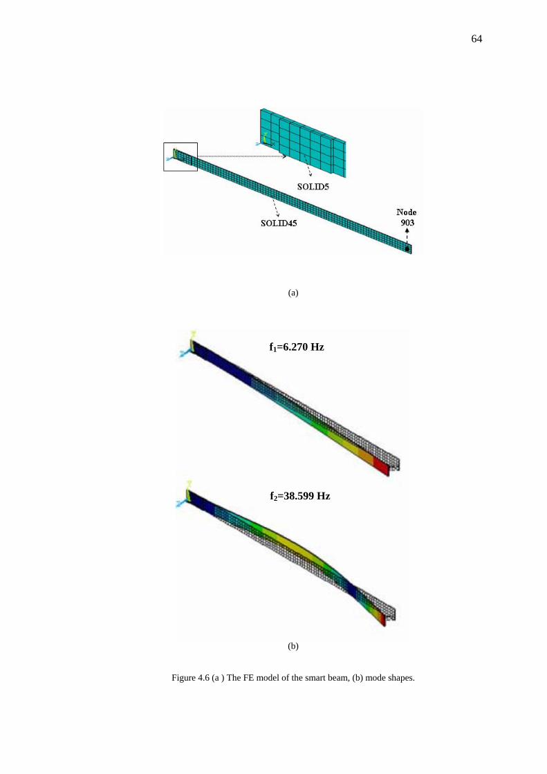
64
(a)
(b)
Figure 4.6 (a ) The FE model of the smart beam, (b) mode shapes.
f1=6.270 Hz
f2=38.599 Hz
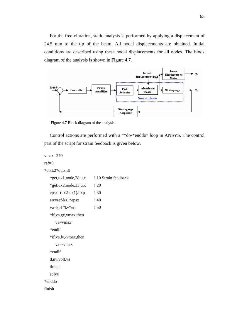
65
For the free vibration, static analysis is performed by applying a displacement of
24.5 mm to the tip of the beam. All nodal displacements are obtained. Initial
conditions are described using these nodal displacements for all nodes. The block
diagram of the analysis is shown in Figure 4.7.
Figure 4.7 Block diagram of the analysis.
Control actions are performed with a “*do-*enddo” loop in ANSYS. The control
part of the script for strain feedback is given below. vmax=270
ref=0
*do,t,2*dt,ts,dt
*get,ux1,node,28,u,x ! 10 Strain feedback
*get,ux2,node,33,u,x ! 20
epsx=(ux2-ux1)/dxp ! 30
err=ref-ks1*epsx ! 40
va=kp1*kv*err ! 50
*if,va,ge,vmax,then
va=vmax
*endif
*if,va,le,-vmax,then
va=-vmax
*endif
d,nv,volt,va
time,t
solve
*enddo
finish
66
The time step dt is found from 1/20*f1, where f1 is the first natural frequency. The
time ts is the analysis time corresponding to nearly steady-state. The first mode of the
vibration is considered in the closed loop control analysis. Strain value epsx in the x
direction is calculated in each step after nodal displacements ux1 and ux2
corresponding to the nodes 28 (L=25 mm, B=10 mm) and 33 (L=30 mm, B=10 mm)
in the FE model are obtained. The response node corresponds to the node 903
(L=440 mm, B=10 mm) in the FE model. The actuation signals va are calculated
after the error signals err are obtained.
The variables Ks1 and Kp1 belong to strain feedback analysis. Ks1 corresponding to
strain gage amplifier in the block diagram is chosen by inspection and provided by
LabVIEW program in the experiment. The variable Kp1 is proportional controller
gain for strain feedback. The variable vmax in the script indicates a saturation value
since the output of the HVPA is limited to ±270 V in the experiment. The saturation
is provided with “*if-*endif” condition statements in the control loop. In order to
compare the simulation results with the experimental results shown in Figure 4.5(a),
the simulation results for Control OFF, Control ON and actuation signals are shown
in Figure 4.8.
For the displacement feedback, the lines numbered (!10, !20, !30, !40 and !50) in
the control part of the script are replaced with the lines described below. *get,uztip,node,903,u,z ! Displacement feedback
err=ref-ks2*uztip
va=kp2*kv*err
The node 903 (L=440 mm, B= 10 mm) is considered as both the feedback and the
response node. The variables Ks2 and Kp2 belong to displacement feedback analysis.
Displacement values are converted to voltage values by Ks2 to obtain feedback signal
as mentioned in the experimental work in section 2. The variable Kp2 is proportional
controller gain for displacement feedback. The variable Kv is common for the two
feedback analyses and corresponds to HVPA in the experiment. The variables Kv, Ks1
and Ks2 are constants in the analysis and taken as 30, 10000 and 250, respectively.
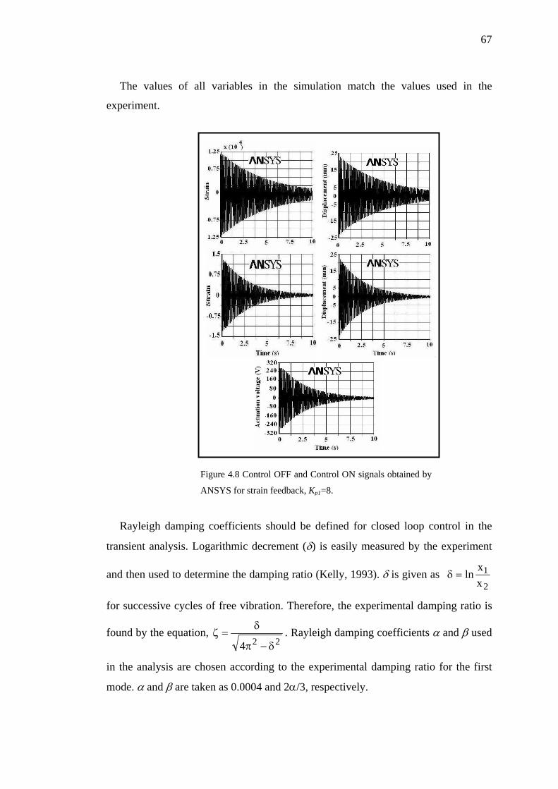
67
The values of all variables in the simulation match the values used in the
experiment.
Rayleigh damping coefficients should be defined for closed loop control in the
transient analysis. Logarithmic decrement (δ) is easily measured by the experiment
and then used to determine the damping ratio (Kelly, 1993). δ is given as 2
1xx
ln=δ
for successive cycles of free vibration. Therefore, the experimental damping ratio is
found by the equation, 224 δ−π
δ=ζ . Rayleigh damping coefficients α and β used
in the analysis are chosen according to the experimental damping ratio for the first
mode. α and β are taken as 0.0004 and 2α/3, respectively.
Figure 4.8 Control OFF and Control ON signals obtained by
ANSYS for strain feedback, Kp1=8.
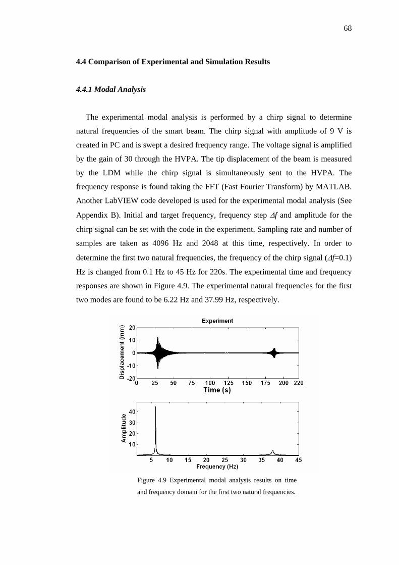
68
4.4 Comparison of Experimental and Simulation Results
4.4.1 Modal Analysis
The experimental modal analysis is performed by a chirp signal to determine
natural frequencies of the smart beam. The chirp signal with amplitude of 9 V is
created in PC and is swept a desired frequency range. The voltage signal is amplified
by the gain of 30 through the HVPA. The tip displacement of the beam is measured
by the LDM while the chirp signal is simultaneously sent to the HVPA. The
frequency response is found taking the FFT (Fast Fourier Transform) by MATLAB.
Another LabVIEW code developed is used for the experimental modal analysis (See
Appendix B). Initial and target frequency, frequency step Δf and amplitude for the
chirp signal can be set with the code in the experiment. Sampling rate and number of
samples are taken as 4096 Hz and 2048 at this time, respectively. In order to
determine the first two natural frequencies, the frequency of the chirp signal (Δf=0.1)
Hz is changed from 0.1 Hz to 45 Hz for 220s. The experimental time and frequency
responses are shown in Figure 4.9. The experimental natural frequencies for the first
two modes are found to be 6.22 Hz and 37.99 Hz, respectively.
Figure 4.9 Experimental modal analysis results on time
and frequency domain for the first two natural frequencies.
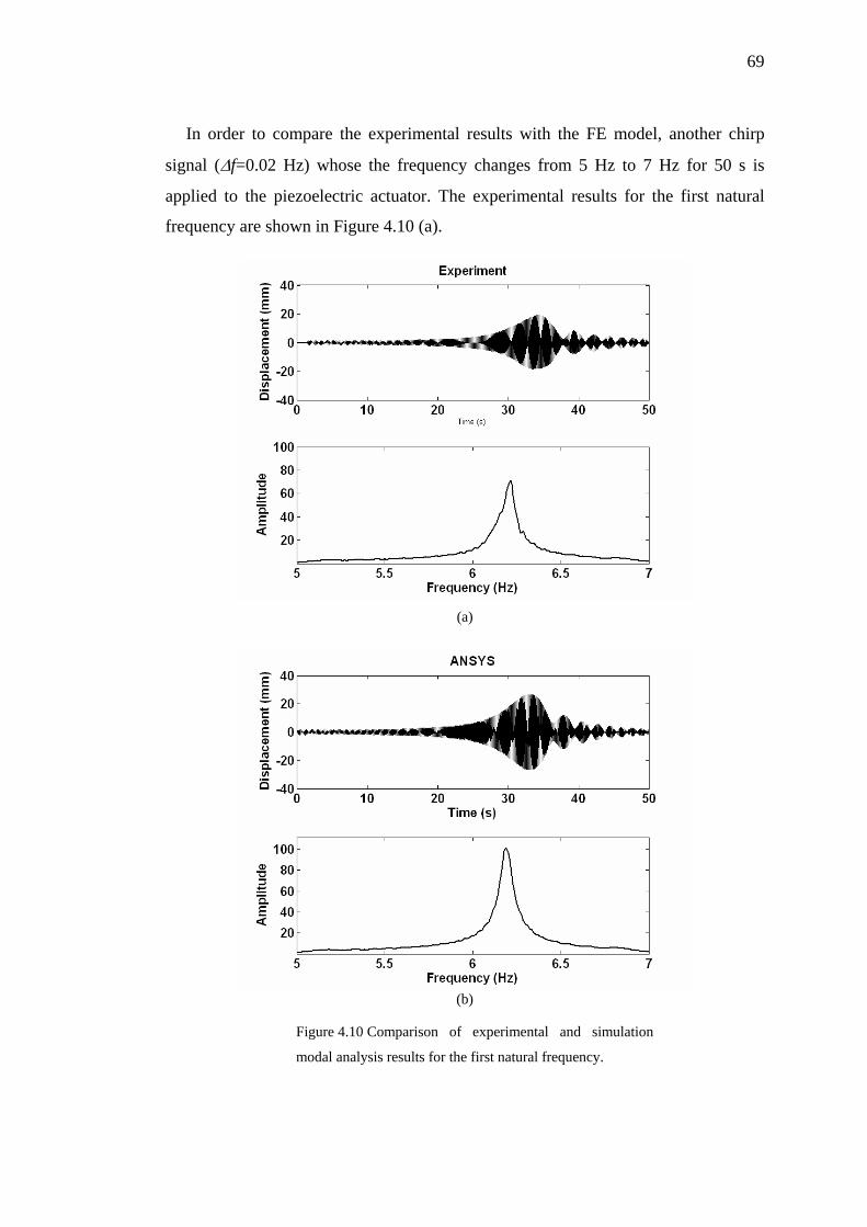
69
In order to compare the experimental results with the FE model, another chirp
signal (Δf=0.02 Hz) whose the frequency changes from 5 Hz to 7 Hz for 50 s is
applied to the piezoelectric actuator. The experimental results for the first natural
frequency are shown in Figure 4.10 (a).
(a)
(b)
Figure 4.10 Comparison of experimental and simulation
modal analysis results for the first natural frequency.
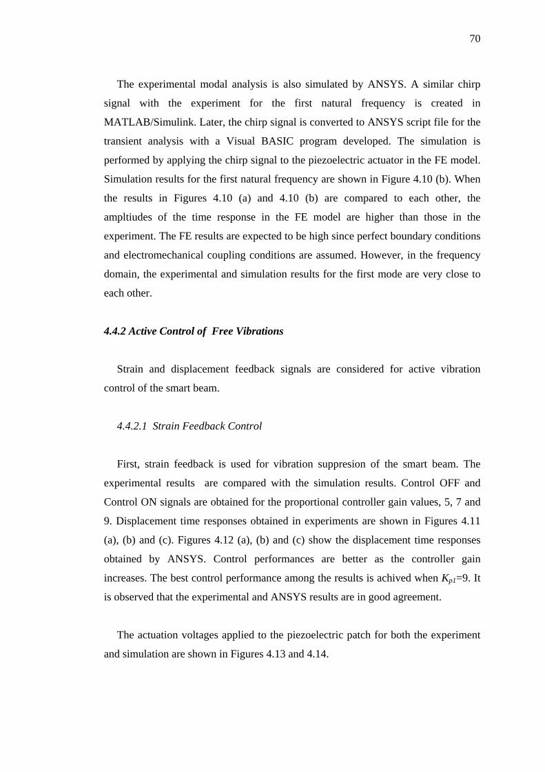
70
The experimental modal analysis is also simulated by ANSYS. A similar chirp
signal with the experiment for the first natural frequency is created in
MATLAB/Simulink. Later, the chirp signal is converted to ANSYS script file for the
transient analysis with a Visual BASIC program developed. The simulation is
performed by applying the chirp signal to the piezoelectric actuator in the FE model.
Simulation results for the first natural frequency are shown in Figure 4.10 (b). When
the results in Figures 4.10 (a) and 4.10 (b) are compared to each other, the
ampltiudes of the time response in the FE model are higher than those in the
experiment. The FE results are expected to be high since perfect boundary conditions
and electromechanical coupling conditions are assumed. However, in the frequency
domain, the experimental and simulation results for the first mode are very close to
each other.
4.4.2 Active Control of Free Vibrations
Strain and displacement feedback signals are considered for active vibration
control of the smart beam.
4.4.2.1 Strain Feedback Control
First, strain feedback is used for vibration suppresion of the smart beam. The
experimental results are compared with the simulation results. Control OFF and
Control ON signals are obtained for the proportional controller gain values, 5, 7 and
9. Displacement time responses obtained in experiments are shown in Figures 4.11
(a), (b) and (c). Figures 4.12 (a), (b) and (c) show the displacement time responses
obtained by ANSYS. Control performances are better as the controller gain
increases. The best control performance among the results is achived when Kp1=9. It
is observed that the experimental and ANSYS results are in good agreement.
The actuation voltages applied to the piezoelectric patch for both the experiment
and simulation are shown in Figures 4.13 and 4.14.
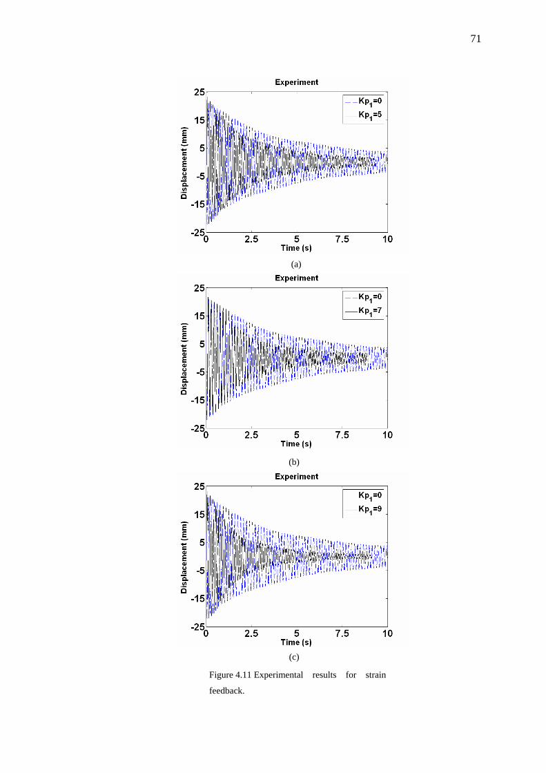
71
(a)
(b)
(c)
Figure 4.11 Experimental results for strain
feedback.
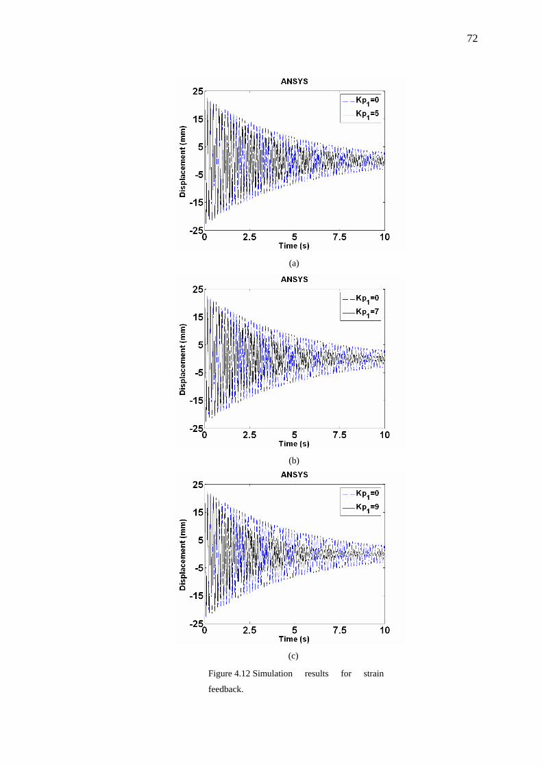
72
(a)
(b)
(c)
Figure 4.12 Simulation results for strain
feedback.
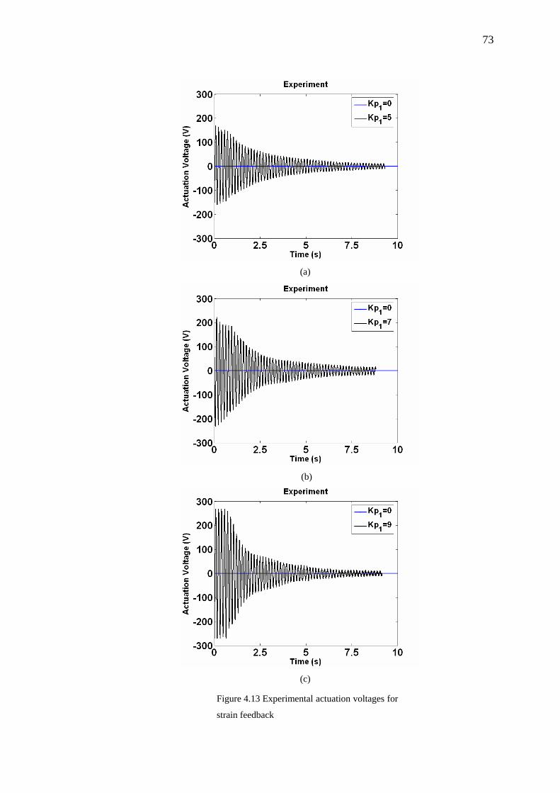
73
(a)
(b)
(c)
Figure 4.13 Experimental actuation voltages for
strain feedback
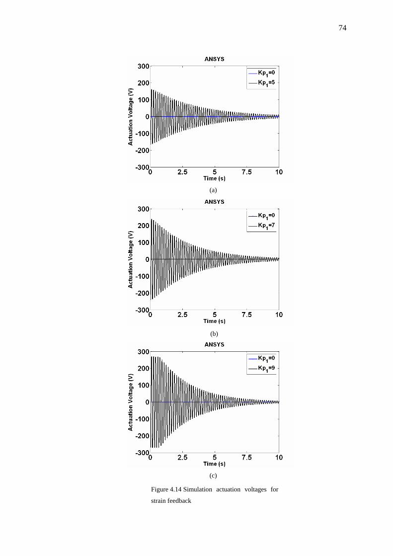
74
(a)
(b)
(c)
Figure 4.14 Simulation actuation voltages for
strain feedback
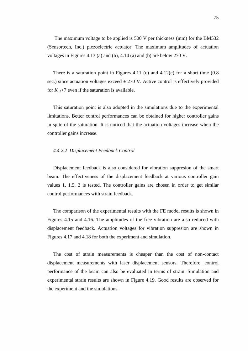
75
The maximum voltage to be applied is 500 V per thickness (mm) for the BM532
(Sensortech, Inc.) piezoelectric actuator. The maximum amplitudes of actuation
voltages in Figures 4.13 (a) and (b), 4.14 (a) and (b) are below 270 V.
There is a saturation point in Figures 4.11 (c) and 4.12(c) for a short time (0.8
sec.) since actuation voltages exceed ± 270 V. Active control is effectively provided
for Kp1>7 even if the saturation is available.
This saturation point is also adopted in the simulations due to the experimental
limitations. Better control performances can be obtained for higher controller gains
in spite of the saturation. It is noticed that the actuation voltages increase when the
controller gains increase.
4.4.2.2 Displacement Feedback Control
Displacement feedback is also considered for vibration suppresion of the smart
beam. The effectiveness of the displacement feedback at various controller gain
values 1, 1.5, 2 is tested. The controller gains are chosen in order to get similar
control performances with strain feedback.
The comparison of the experimental results with the FE model results is shown in
Figures 4.15 and 4.16. The amplitudes of the free vibration are also reduced with
displacement feedback. Actuation voltages for vibration suppresion are shown in
Figures 4.17 and 4.18 for both the experiment and simulation.
The cost of strain measurements is cheaper than the cost of non-contact
displacement measurements with laser displacement sensors. Therefore, control
performance of the beam can also be evaluated in terms of strain. Simulation and
experimental strain results are shown in Figure 4.19. Good results are observed for
the experiment and the simulations.
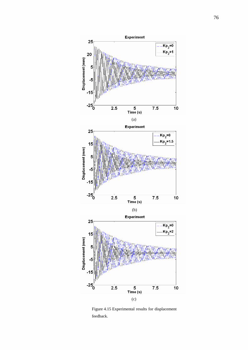
76
(a)
(b)
(c)
Figure 4.15 Experimental results for displacement
feedback.

77
(a)
(b)
(c)
Figure 4.16 Simulation results for displacement
feedback.
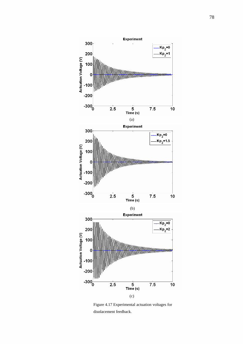
78
(a)
(b)
(c)
Figure 4.17 Experimental actuation voltages for
displacement feedback.
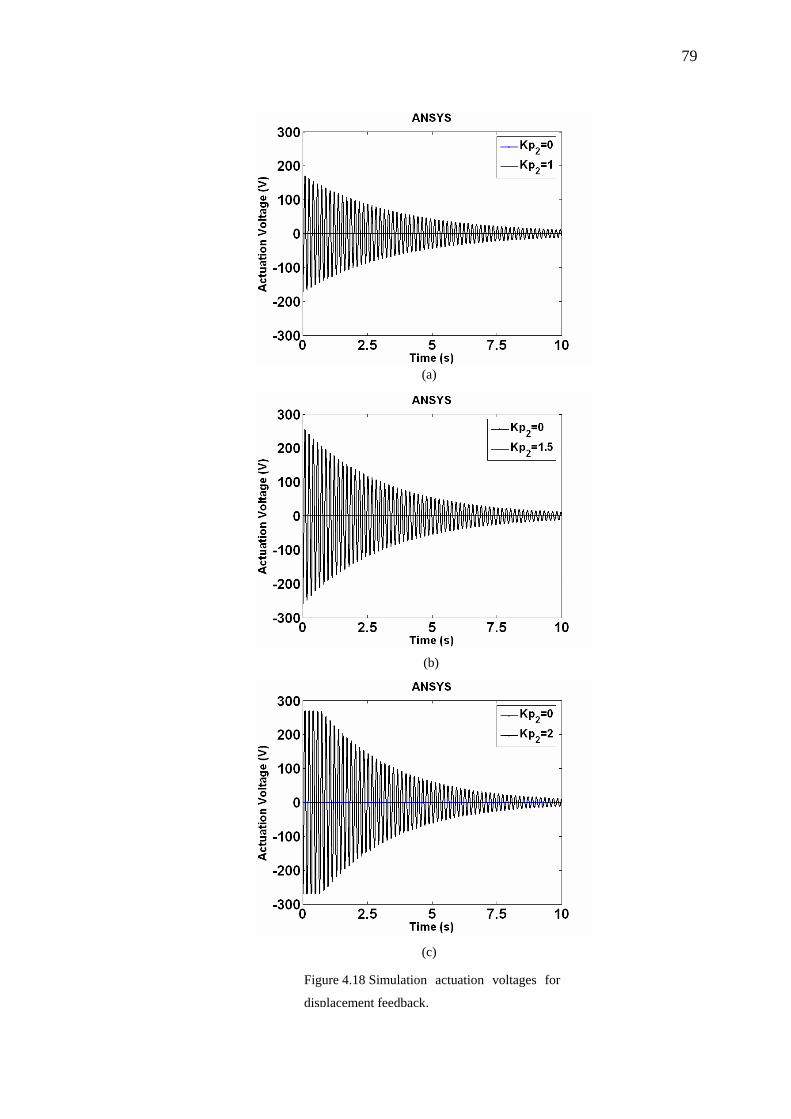
79
(a)
(b)
(c)
Figure 4.18 Simulation actuation voltages for
displacement feedback.
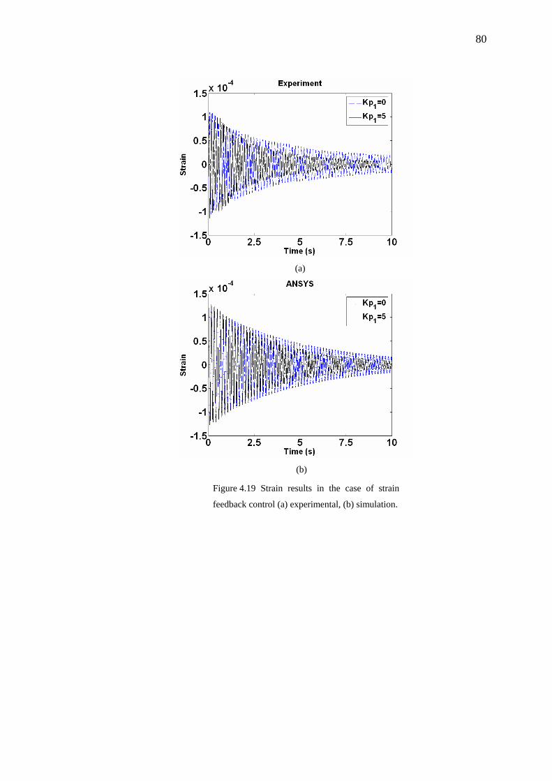
80
(a)
(b)
Figure 4.19 Strain results in the case of strain
feedback control (a) experimental, (b) simulation.
81
CHAPTER FIVE
SIMULATION AND EXPERIMENTAL ANALYSIS OF ACTIVE
VIBRATION CONTROL OF SMART BEAMS UNDER
HARMONIC EXCITATION
5.1 Introduction
In this chapter, the active control of a smart beam under forced vibration is
analyzed. The aluminum smart beam is composed of two piezoelectric (Lead-
Zirconate-Titanate) patches and strain gage. One of the piezoelectric patches is used
as controlling actuator while the other piezoelectric patch is used as vibration
generating shaker. The smart beam is harmonically excited by the piezoelectric
shaker at its fundamental frequency. The strain gage is utilized to sense the vibration
level. Active vibration reduction under harmonic excitation is achieved using both
strain and displacement feedback control.
Closed loop simulations are performed by APDL while experimental applications
are performed by LabVIEW. Dynamic behaviour at the tip of the beam is evaluated
for the uncontrolled and controlled responses. The simulation and experimental
results are compared. It is observed that good agreement is observed between
simulation and experimental results under harmonic excitation.
5.2 Active Control of Forced Vibrations
Smart structures with metal and piezoelectric sections can be modeled by
ANSYS. Three dimensional structural element (SOLID45) is used for the metal part
of the smart beam. The piezoelectric patches are modeled using three dimensional
coupled elements (SOLID5). The features of the elements used in the analysis, the
constitutive equations for the piezoelectric materials and the FE formulation for the
coupled field analysis are introduced in chapter 1.
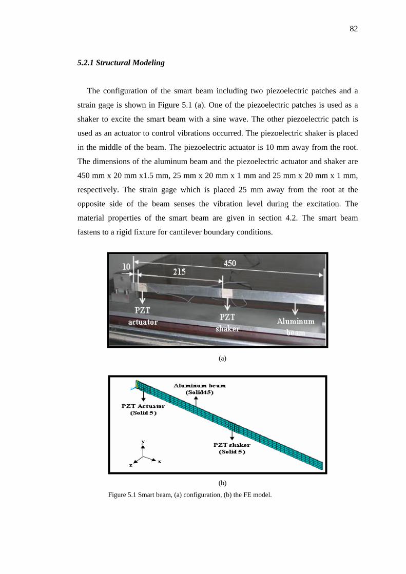
82
5.2.1 Structural Modeling
The configuration of the smart beam including two piezoelectric patches and a
strain gage is shown in Figure 5.1 (a). One of the piezoelectric patches is used as a
shaker to excite the smart beam with a sine wave. The other piezoelectric patch is
used as an actuator to control vibrations occurred. The piezoelectric shaker is placed
in the middle of the beam. The piezoelectric actuator is 10 mm away from the root.
The dimensions of the aluminum beam and the piezoelectric actuator and shaker are
450 mm x 20 mm x1.5 mm, 25 mm x 20 mm x 1 mm and 25 mm x 20 mm x 1 mm,
respectively. The strain gage which is placed 25 mm away from the root at the
opposite side of the beam senses the vibration level during the excitation. The
material properties of the smart beam are given in section 4.2. The smart beam
fastens to a rigid fixture for cantilever boundary conditions.
(a)
(b)
Figure 5.1 Smart beam, (a) configuration, (b) the FE model.
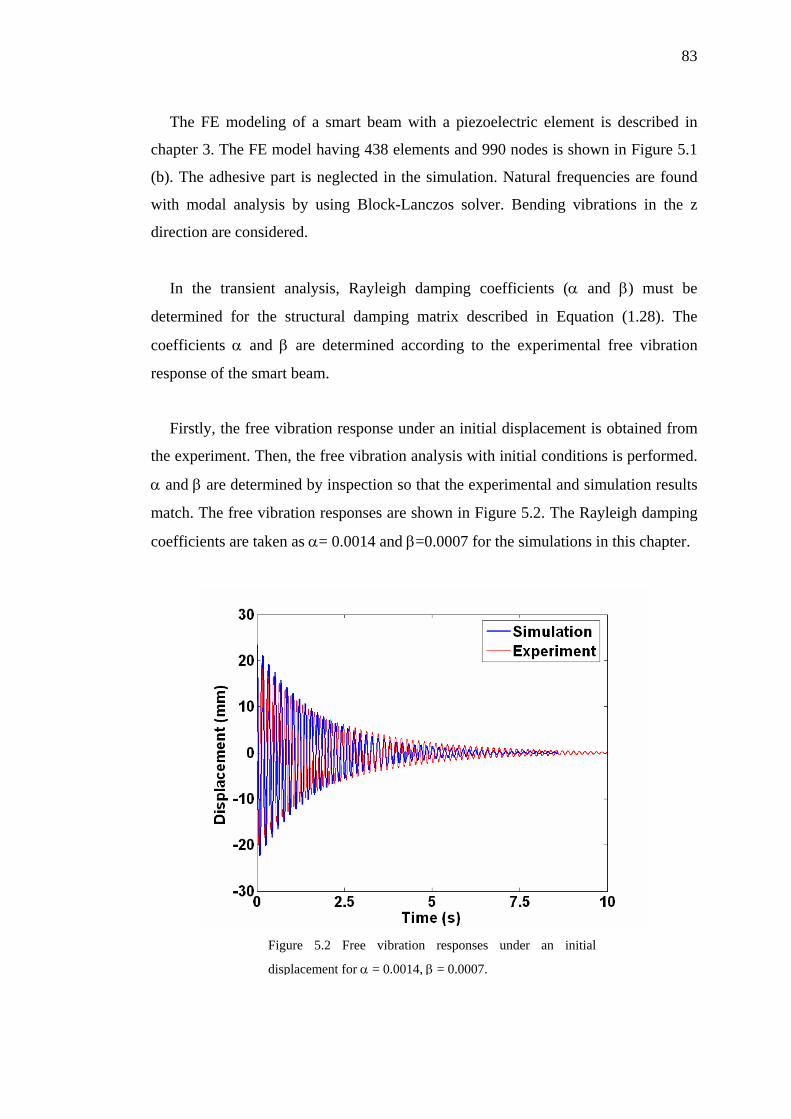
83
The FE modeling of a smart beam with a piezoelectric element is described in
chapter 3. The FE model having 438 elements and 990 nodes is shown in Figure 5.1
(b). The adhesive part is neglected in the simulation. Natural frequencies are found
with modal analysis by using Block-Lanczos solver. Bending vibrations in the z
direction are considered.
In the transient analysis, Rayleigh damping coefficients (α and β) must be
determined for the structural damping matrix described in Equation (1.28). The
coefficients α and β are determined according to the experimental free vibration
response of the smart beam.
Firstly, the free vibration response under an initial displacement is obtained from
the experiment. Then, the free vibration analysis with initial conditions is performed.
α and β are determined by inspection so that the experimental and simulation results
match. The free vibration responses are shown in Figure 5.2. The Rayleigh damping
coefficients are taken as α= 0.0014 and β=0.0007 for the simulations in this chapter.
Figure 5.2 Free vibration responses under an initial
displacement for α = 0.0014, β = 0.0007.
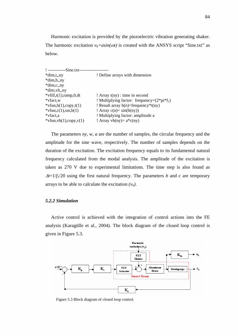
84
Harmonic excitation is provided by the piezoelectric vibration generating shaker.
The harmonic excitation vh=asin(ωt) is created with the ANSYS script “Sine.txt” as
below.
! ------------Sine.txt-------------------- *dim,t,,ny ! Define arrays with dimension *dim,b,,ny *dim,c,,ny *dim,vh,,ny *vfill,t(1),ramp,0,dt ! Array t(ny) : time in second *vfact,w ! Multiplying factor: frequency=(2*pi*f1) *vfun,b(1),copy,t(1) ! Result array b(n)=frequency*t(ny) *vfun,c(1),sın,b(1) ! Array c(n)= sin(b(ny)) *vfact,a ! Multiplying factor: amplitude a *vfun,vh(1),copy,c(1) ! Array vh(ny)= a*c(ny)
The parameters ny, w, a are the number of samples, the circular frequency and the
amplitude for the sine wave, respectively. The number of samples depends on the
duration of the excitation. The excitation frequency equals to its fundamental natural
frequency calculated from the modal analysis. The amplitude of the excitation is
taken as 270 V due to experimental limitations. The time step is also found as
Δt=1/f1/20 using the first natural frequency. The parameters b and c are temporary
arrays to be able to calculate the excitation (vh).
5.2.2 Simulation
Active control is achieved with the integration of control actions into the FE
analysis (Karagülle et al., 2004). The block diagram of the closed loop control is
given in Figure 5.3.
Figure 5.3 Block diagram of closed loop control.
85
Control actions are performed with the script code after the FE model of the smart
beam is constructed (See Appendix C). The analysis of active control is carried out
by the following scripts.
/input,sine,txt
d,nsv,volt,vh(1)
time,dt
solve
r=0
*do,i,2,ny
d,961,volt,vh(i)
*get,ux1,node,28,,u,x
*get,ux2,node,33,u,x
epsx=(ux2-ux1)/dxp
err=r-ks*epsx
va=kp*kv*err
d,nv,volt,va
time,i*dt
solve
*enddo
Harmonic excitation is created in the file “sine.txt” before the control loop is
initiated. The first step is solved applying the excitation voltage (node 961) to the
piezoelectric shaker. Hence, the nodal solutions of the FE model are known for the
next step.
Active control is realized in “*do-*enddo” loop. The excitation is applied again in
the first line of the control loop. The elongations ux1 (node 28) and ux2 (node 33)
known from the first step are read from the nodes corresponding to the strain gage
location. Error signal is obtained after the strain value is calculated. Strain value is
multiplied by Ks to provide optimum control performance.
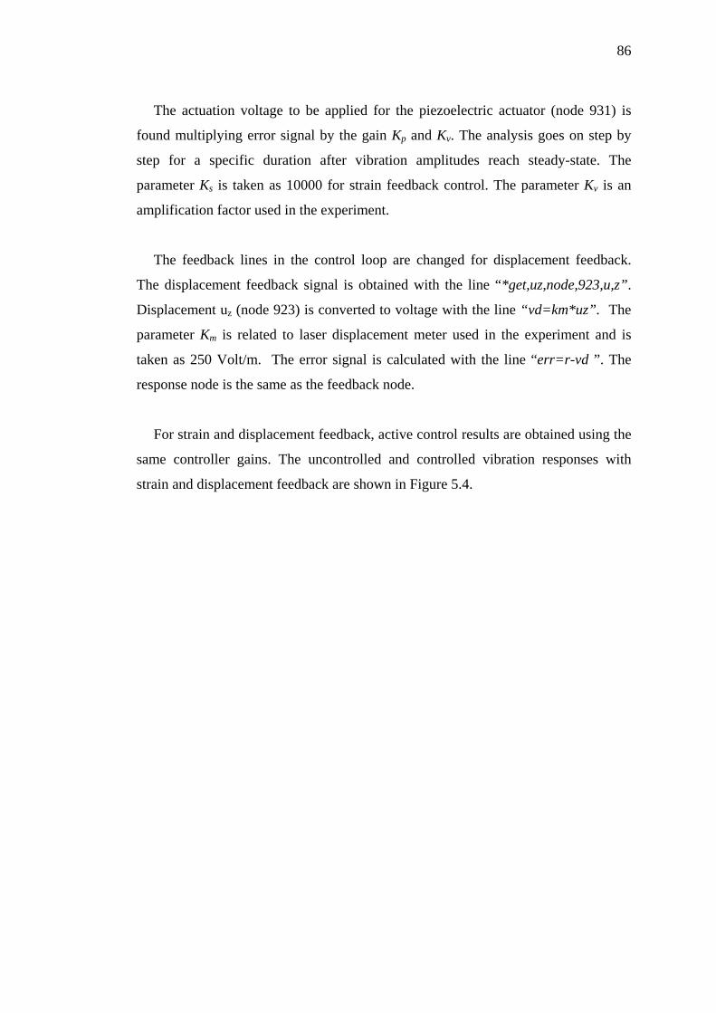
86
The actuation voltage to be applied for the piezoelectric actuator (node 931) is
found multiplying error signal by the gain Kp and Kv. The analysis goes on step by
step for a specific duration after vibration amplitudes reach steady-state. The
parameter Ks is taken as 10000 for strain feedback control. The parameter Kv is an
amplification factor used in the experiment.
The feedback lines in the control loop are changed for displacement feedback.
The displacement feedback signal is obtained with the line “*get,uz,node,923,u,z”.
Displacement uz (node 923) is converted to voltage with the line “vd=km*uz”. The
parameter Km is related to laser displacement meter used in the experiment and is
taken as 250 Volt/m. The error signal is calculated with the line “err=r-vd ”. The
response node is the same as the feedback node.
For strain and displacement feedback, active control results are obtained using the
same controller gains. The uncontrolled and controlled vibration responses with
strain and displacement feedback are shown in Figure 5.4.
87
(a)
(b)
(c) Figure 5.4 Simulation results with sine wave of
6.12 Hz, (a) uncontrolled response, (b) controlled
response with strain feedback, (c) controlled
response with displacement feedback.
Transient Steady-state
88
5.2.3 Experiment
As explained previously, the natural frequencies, uncontrolled and controlled time
responses of a cantilever smart beam can be predicted with the simulations.
Experimental modal analysis and experimental closed loop control is conducted to
verify the simulation results. In active control of forced vibrations, a smart beam
having a different configuration is produced bonding two piezoelectric patches to the
aluminum beam with conductive epoxy (See Figure 5.1). The piezoelectric actuator
is placed near the root of the beam to perform effective control. The piezoelectric
shaker placed in the middle of the beam generates harmonic excitation. The ground
connections of the two patches are different. The ground connection of the
piezoelectric actuator is on aluminum beam while that of the piezoelectric shaker is
its back side since it is isolated from the beam. Sensortech BM532 patches are used
for the piezoelectric actuators. The material properties of the piezoelectric and
aluminum beam are presented in Table 4.2. The strain gage which is bonded to the
beam at the opposite side of the piezoelectric patches measures the vibration level.
Experimental system introduced in the previous chapter is used for the
experiments. Experimental system consists of a smart beam, straingauge input
module, a signal conditioning unit, a non-contact laser displacement sensor, high
voltage power amplifiers, multifunction data acquisition cards and a personal
computer programming with LabVIEW. A LabVIEW program is developed to
control of the smart beam under harmonic excitation. Two channels of the analog
output card are programmed. One of the channels is used to provide harmonic
excitation to the power amplifier. Other channel is used to provide control signal the
piezoelectric actuator over the other power amplifier. Two power amplifiers (SA-10)
are utilized for the excitation and control. A digital low pass filter of 30 Hz is used
during the strain and displacement measurements.
The uncontrolled and controlled vibration responses under harmonic excitation
obtained by the experiment are shown in Figure 5.5 (See Figure 5.4).
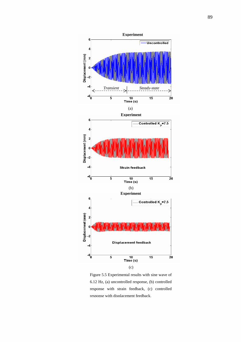
89
Experiment
Transient Steady-state
Experiment
Experiment
(a)
(b)
(c)
Figure 5.5 Experimental results with sine wave of
6.12 Hz, (a) uncontrolled response, (b) controlled
response with strain feedback, (c) controlled
response with displacement feedback.
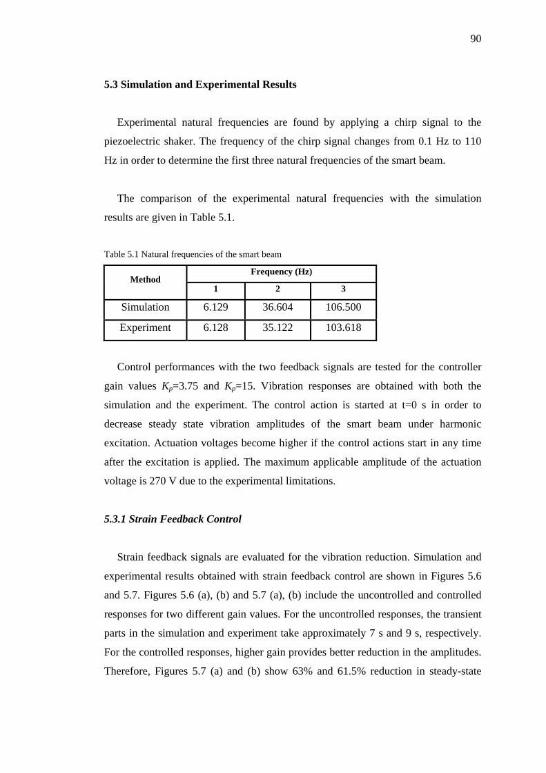
90
5.3 Simulation and Experimental Results
Experimental natural frequencies are found by applying a chirp signal to the
piezoelectric shaker. The frequency of the chirp signal changes from 0.1 Hz to 110
Hz in order to determine the first three natural frequencies of the smart beam.
The comparison of the experimental natural frequencies with the simulation
results are given in Table 5.1.
Table 5.1 Natural frequencies of the smart beam
Frequency (Hz) Method
1 2 3
Simulation 6.129 36.604 106.500
Experiment 6.128 35.122 103.618
Control performances with the two feedback signals are tested for the controller
gain values Kp=3.75 and Kp=15. Vibration responses are obtained with both the
simulation and the experiment. The control action is started at t=0 s in order to
decrease steady state vibration amplitudes of the smart beam under harmonic
excitation. Actuation voltages become higher if the control actions start in any time
after the excitation is applied. The maximum applicable amplitude of the actuation
voltage is 270 V due to the experimental limitations.
5.3.1 Strain Feedback Control
Strain feedback signals are evaluated for the vibration reduction. Simulation and
experimental results obtained with strain feedback control are shown in Figures 5.6
and 5.7. Figures 5.6 (a), (b) and 5.7 (a), (b) include the uncontrolled and controlled
responses for two different gain values. For the uncontrolled responses, the transient
parts in the simulation and experiment take approximately 7 s and 9 s, respectively.
For the controlled responses, higher gain provides better reduction in the amplitudes.
Therefore, Figures 5.7 (a) and (b) show 63% and 61.5% reduction in steady-state
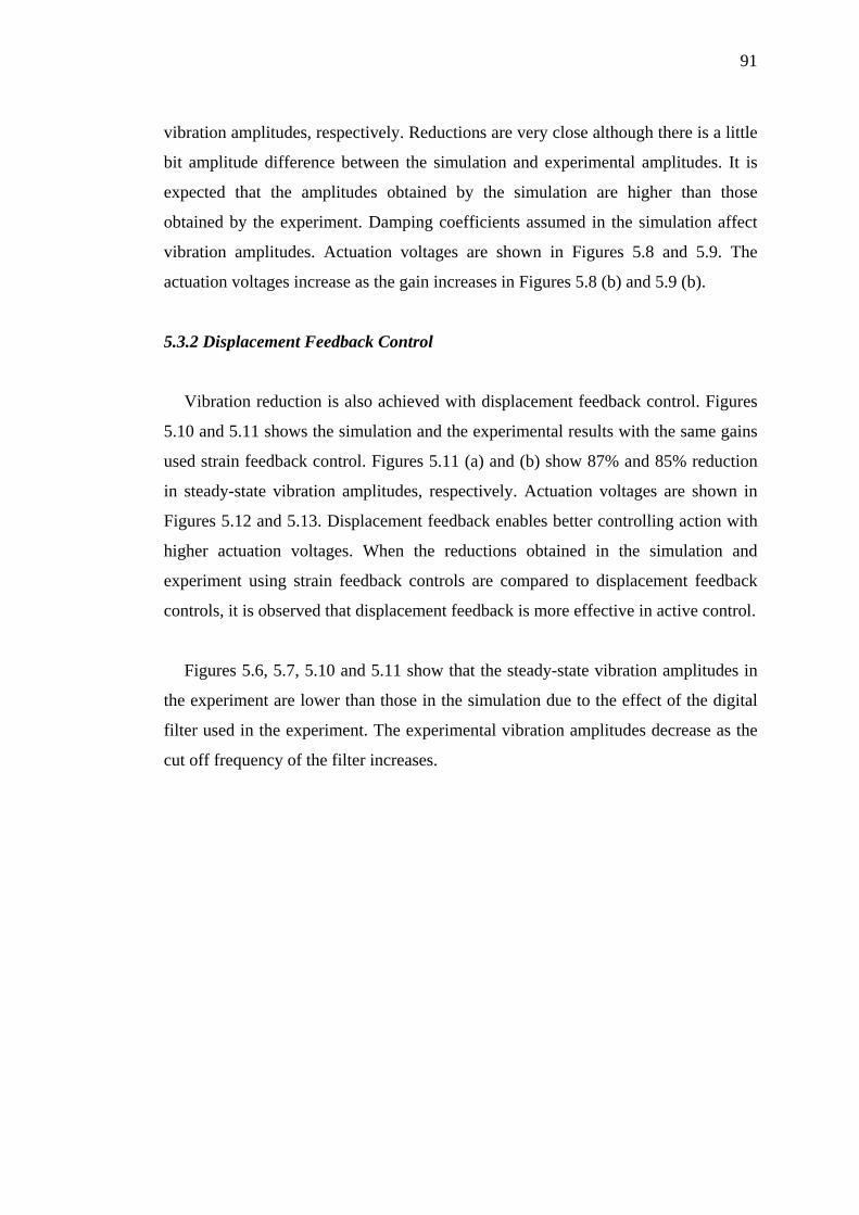
91
vibration amplitudes, respectively. Reductions are very close although there is a little
bit amplitude difference between the simulation and experimental amplitudes. It is
expected that the amplitudes obtained by the simulation are higher than those
obtained by the experiment. Damping coefficients assumed in the simulation affect
vibration amplitudes. Actuation voltages are shown in Figures 5.8 and 5.9. The
actuation voltages increase as the gain increases in Figures 5.8 (b) and 5.9 (b).
5.3.2 Displacement Feedback Control
Vibration reduction is also achieved with displacement feedback control. Figures
5.10 and 5.11 shows the simulation and the experimental results with the same gains
used strain feedback control. Figures 5.11 (a) and (b) show 87% and 85% reduction
in steady-state vibration amplitudes, respectively. Actuation voltages are shown in
Figures 5.12 and 5.13. Displacement feedback enables better controlling action with
higher actuation voltages. When the reductions obtained in the simulation and
experiment using strain feedback controls are compared to displacement feedback
controls, it is observed that displacement feedback is more effective in active control.
Figures 5.6, 5.7, 5.10 and 5.11 show that the steady-state vibration amplitudes in
the experiment are lower than those in the simulation due to the effect of the digital
filter used in the experiment. The experimental vibration amplitudes decrease as the
cut off frequency of the filter increases.
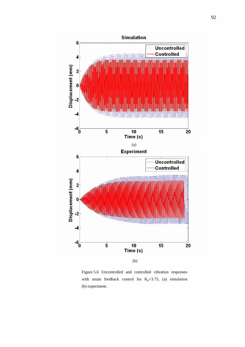
92
(a)
(b)
Figure 5.6 Uncontrolled and controlled vibration responses
with strain feedback control for Kp=3.75, (a) simulation
(b) experiment.
93
(a)
(b)
Figure 5.7 Uncontrolled and controlled vibration responses
with strain feedback control for Kp=15, (a) simulation,
(b) experiment.
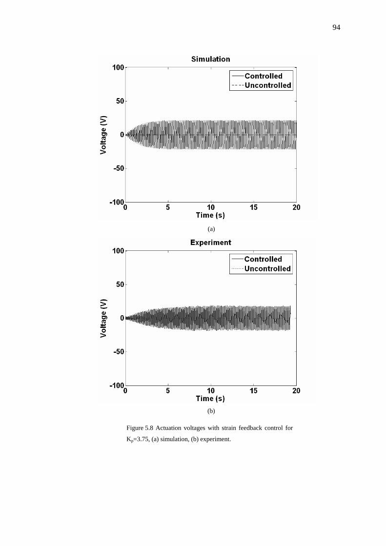
94
(a)
(b)
Figure 5.8 Actuation voltages with strain feedback control for
Kp=3.75, (a) simulation, (b) experiment.
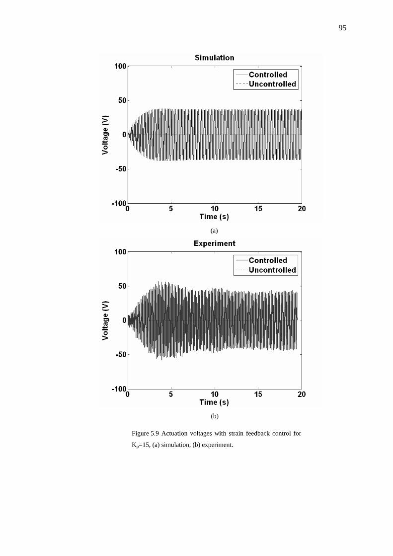
95
(a)
(b)
Figure 5.9 Actuation voltages with strain feedback control for
Kp=15, (a) simulation, (b) experiment.
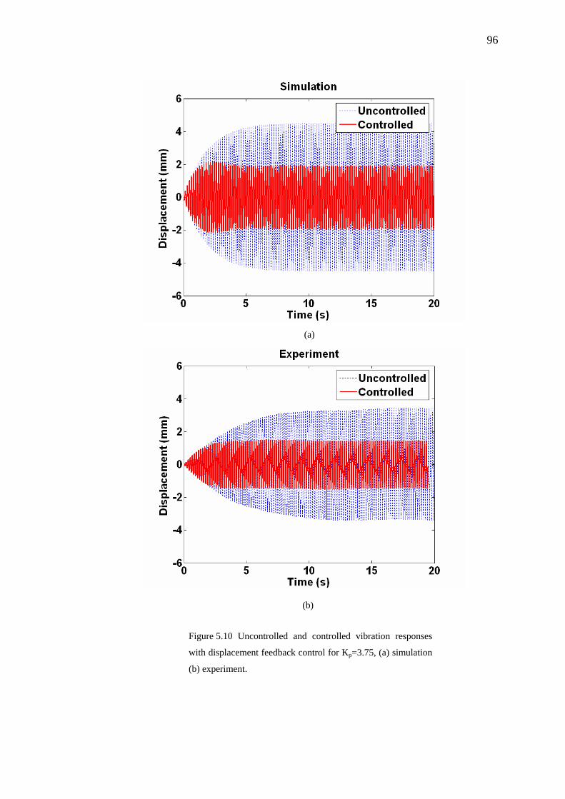
96
(a)
(b)
Figure 5.10 Uncontrolled and controlled vibration responses
with displacement feedback control for Kp=3.75, (a) simulation
(b) experiment.
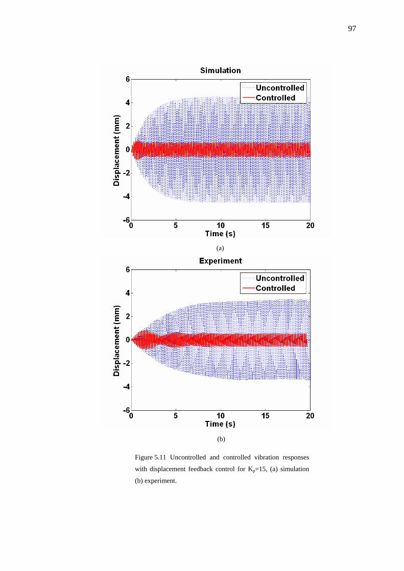
97
(a)
(b)
Figure 5.11 Uncontrolled and controlled vibration responses
with displacement feedback control for Kp=15, (a) simulation
(b) experiment.
98
(a)
(b)
Figure 5.12 Actuation voltages with displacement feedback
control for Kp=3.75, (a) simulation, (b) experiment.
99
(a)
(b)
Figure 5.13 Actuation voltages with displacement feedback
control for Kp=15, (a) simulation, (b) experiment.
100
CHAPTER SIX
ANALYSIS OF ACTIVE VIBRATION CONTROL OF SMART BEAMS
SUBJECTED TO MOVING LOAD
6.1 Introduction
This chapter includes two main parts. Numerical and experimental vibration
analyses of the aluminum beam subjected to moving load are presented at first. Then,
active control of smart beams having different configurations under moving load is
investigated by the closed loop simulations.
In the first part of this chapter, experimental system for moving load is
introduced. In the experiments, motion of the load is provided by using ABB IRB
1400, which is an industrial robot with six degrees of freedom. The load is created by
blowing compressed air to the cantilever beam. Dynamic time responses of the beam
under moving load are measured at two different points by utilizing non-contact
LDS’s. The FE simulations are performed to verify the results of the experimental
beam subjected to moving load.
In the second part of this chapter, active vibration control of piezoelectric smart
beams having different configurations and boundary conditions is studied under
moving load. Two case studies are presented to demonstrate the validity of the
analysis procedure proposed in the thesis. In the first case, the experimental
cantilever beam tested in section 6.2 is studied with two bonded piezoelectric
actuators. Experiments are performed to verify the natural frequencies and the
dynamic behaviour of the cantilever smart beam. In order to reduce vibration
amplitudes due to the moving load, displacement feedback control is studied with the
same loading and velocity parameters considered in the first part. In the second case,
active control of a fixed-fixed smart beam subjected to a moving load is examined.
Strain feedback control is applied to the smart beam having different configurations
such as monomorph and bimorph. Simulation results are presented for the both cases.
101
Vibrations due to moving load have been investigated by engineers in various
engineering fields. Bridges on which vehicles or trains travel, piping systems
subjected to two-phase flow, beams subjected to pressure waves, and machining
operations where high axial speed may be employed, structures on cranes can be
modeled as moving loads on beams with different boundary conditions. A crane
model is studied using beam elements by Wu, Whittaker, & Cartmell (2000). Wu
(2003) also investigated a rectangular plate subjected to curvilinear moving loads.
Fundamental problem of vibration of beams with general boundary conditions
traversed by moving loads is studied by Hilal & Zibdeh (2000). They assumed the
moving load to have three types of velocities, accelerating, decelerating, and
constant. They applied analytical formulation to Euler-Bernoulli beams and also
examined the effect of different boundary conditions and damping. They obtained
dynamic magnification factors (V/V0) versus dimensionless time parameters (S) for
various dimensionless speed parameters (α) and damping ratios (ξ) in beams as
shown in Figure 6.1. Kıral & Karagülle (2002) studied the moving load problem
numerically. They analyzed the dynamic behaviour of a single span beam resting on
a elastic foundation by using I-DEAS.
Figure 6.1 The effect of speed and damping on dynamic
magnification factors versus time ratio for (a-c) a fixed-free
beam, (d-f) a fixed-fixed beam, (Hilal & Zibdeh, 2000).
102
Lam & Ng (1999) studied active control of composite plates with piezoelectric
patches under dynamic loading conditions. The composite plate with piezoelectric
sensor and actuator layers considered is shown in Figure 6.2.
Figure 6.2.Composite plate model, (Lam & Ng 1999).
They presented theoretical formulations based on the classical laminated plate
theory (CLPT) and Navier solutions for smart composite plates. A negative-force-
cum-moment feedback control is applied for the closed loop control of the smart
structure. They obtained the results (Figure 6.3) in terms of dimensionless transverse
deflection at the center of the plate (wdyn/wst) for various dimensionless speed
parameters ( ∞v ). Similar results given in Figures 6.1 and 6.3 will be obtained in the
following sections.
Figure 6.3 Deflection ratios under a moving load for various speeds and controller gain
values for a simply supported square plate, (Lam & Ng 1999).
h h
103
6.2 Vibration Analysis of a Beam Subjected to Moving Load
6.2.1 Experiments
Experimental system used in this study is schematically shown in Figure 6.4.
Dimensions of the cantilever aluminum beam are 1000 mm x 20 mm x 1.5 mm. The
load with constant amplitude and uniform velocity is moved along the beam (from 0
mm to 1000 mm). Dynamic time responses of the beam are measured simultaneously
at points A and B. Laser displacement sensor (LDS) at point A is placed 100 mm
away from the free end while the other LDS at point B is placed 100 mm away from
the root.
Figure 6.4 Schematic view of the experimental system.
104
Specifications of LDS’s are given in Table 6.1. LDS’s are connected to the laser
controller which enables to display measurement values and to get voltage output at
the same time. Voltage outputs in the range of ± 10 V are acquired with LabVIEW
through the analog input card. For LDS’s A and B, the measurement ranges of ± 40
mm and ± 5 mm correspond to the voltage outputs of ± 10 V in the laser controller.
During the moving load experiments, the displacement values are measured as
negative in the z direction as indicated in Figure 6.4.
Table 6.1 Locations and specifications of LDS’s.
LDS’s Distance from beam (mm) Measurement range (mm) Sensitivity (μm)
LDS A 150 ±40 0.5
LDS B 30 ±5 0.05 μm
The experimental system used in this study is shown in Figure 6.5. For the motion
of the load, an industrial robot ABB IRB 1400 with six degrees of freedom is used
and the nozzle is attached to the end arm of the robot. The ABB robot is moved from
the root of the beam to free end. The load acting on the beam is provided with an air
blower nozzle. The nozzle has a circular cross sectional area. The pressure of
compressed air can be set from 0.1 to 10 bar. The air blower nozzle is the
perpendicular to the beam during the motion of the robot. In the experiments,
dynamic measurements are realized for the values of constant compressed air
pressure of 1.50 bar, 1.75 bar, 2.00 bar and 2.25 bar and for the values of constant
velocities of 0.1 m/s, 0.25 m/s, 0.5 m/s and 1 m/s. A relay circuit is created for the
synchronization of measurement data as shown in Figure 6.6. When the motion of
the load and blowing of the compressed air are started, the circuit is triggered a
digital output signal of 24 V from the ABB robot software. This signal is converted
to a digital input signal of 5 V for measurement system. Therefore, the dynamic
behaviour of the experimental beam is measured simultaneously for different values
of velocity and pressure of compressed air. In order to obtain experimental
displacement time responses, a low pass filter is used in the controller of LDS’s. The
values of the filter for the sensors at point A and B are 30 Hz and 100 Hz,
respectively.
105
(a)
(b)
Figure 6.5 Experimental system (a) general view (b) detailed views.
Filter and directional control valve
Pressure set and display
meter
LDS at point B
Aluminum beam
Cantilever fixture ABB robot (IRB 1400)
Nozzle
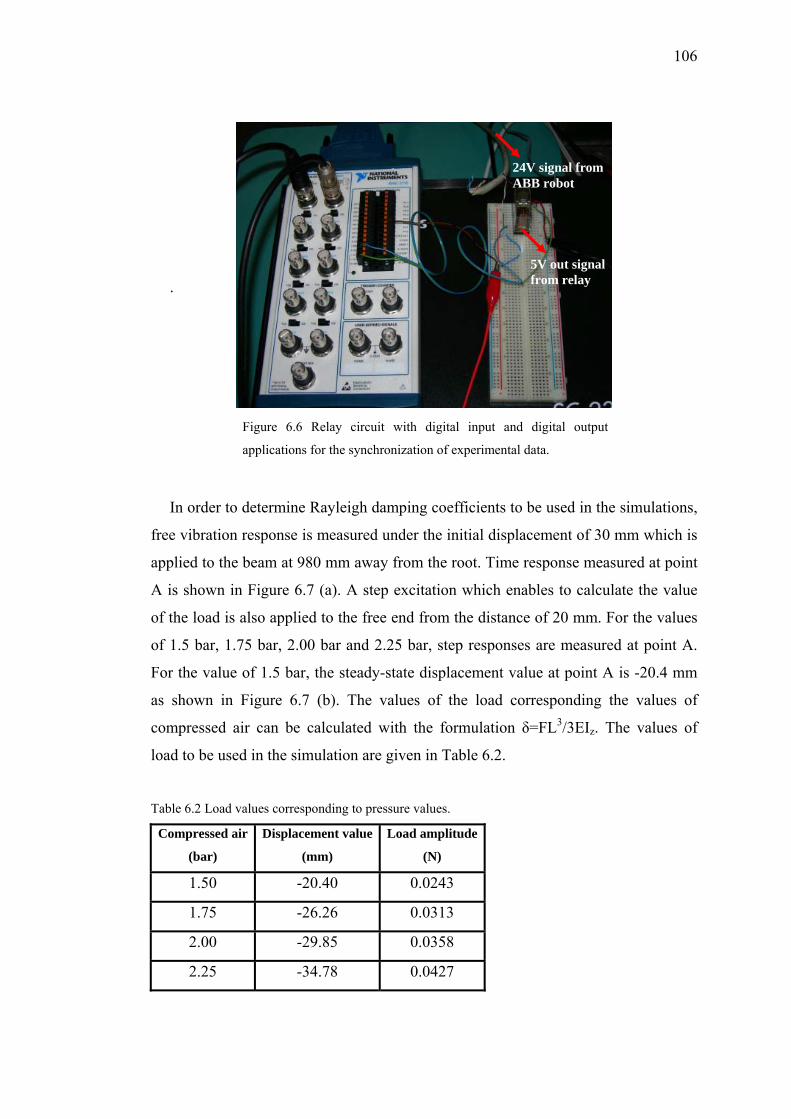
106
.
In order to determine Rayleigh damping coefficients to be used in the simulations,
free vibration response is measured under the initial displacement of 30 mm which is
applied to the beam at 980 mm away from the root. Time response measured at point
A is shown in Figure 6.7 (a). A step excitation which enables to calculate the value
of the load is also applied to the free end from the distance of 20 mm. For the values
of 1.5 bar, 1.75 bar, 2.00 bar and 2.25 bar, step responses are measured at point A.
For the value of 1.5 bar, the steady-state displacement value at point A is -20.4 mm
as shown in Figure 6.7 (b). The values of the load corresponding the values of
compressed air can be calculated with the formulation δ=FL3/3EIz. The values of
load to be used in the simulation are given in Table 6.2.
Table 6.2 Load values corresponding to pressure values.
Compressed air
(bar)
Displacement value
(mm)
Load amplitude
(N)
1.50 -20.40 0.0243
1.75 -26.26 0.0313
2.00 -29.85 0.0358
2.25 -34.78 0.0427
24V signal from ABB robot
5V out signal from relay
Figure 6.6 Relay circuit with digital input and digital output
applications for the synchronization of experimental data.
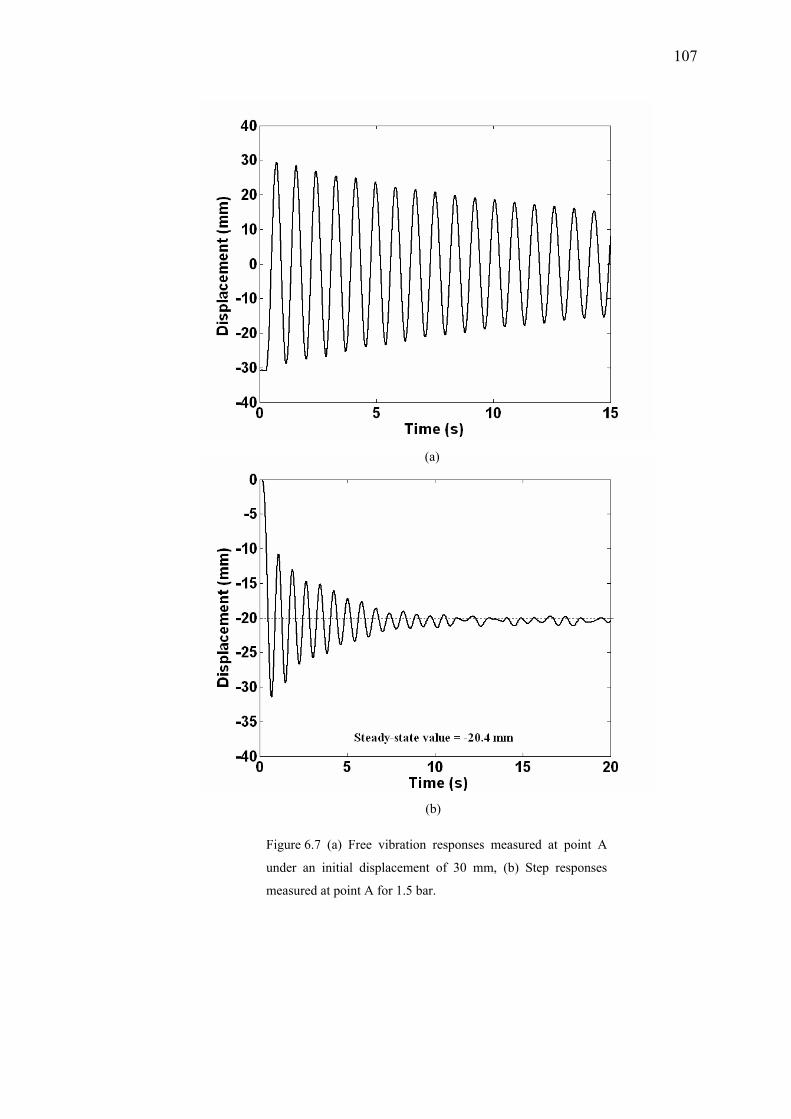
107
(a)
(b)
Figure 6.7 (a) Free vibration responses measured at point A
under an initial displacement of 30 mm, (b) Step responses
measured at point A for 1.5 bar.
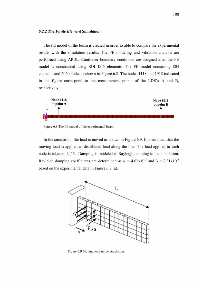
108
Node 1118 at point A
Node 1918 at point B
6.2.2 The Finite Element Simulation
The FE model of the beam is created in order to able to compare the experimental
results with the simulation results. The FE modeling and vibration analysis are
performed using APDL. Cantilever boundary conditions are assigned after the FE
model is constructed using SOLID45 elements. The FE model containing 804
elements and 2020 nodes is shown in Figure 6.8. The nodes 1118 and 1918 indicated
in the figure correspond to the measurement points of the LDS’s A and B,
respectively.
In the simulation, the load is moved as shown in Figure 6.9. It is assumed that the
moving load is applied as distributed load along the line. The load applied to each
node is taken as f0 / 3. Damping is modeled as Rayleigh damping in the simulation.
Rayleigh damping coefficients are determined as α = 4.62x10⁻³ and β = 2.31x10⁻³
based on the experimental data in Figure 6.7 (a).
Figure 6.9 Moving load in the simulation.
Figure 6.8 The FE model of the experimental beam.
109
6.2.3 Experimental and Simulation Results
Modal analysis is done by using the Block Lanczos solver before performing the
dynamic analysis. The first two natural frequencies obtained by the simulation are
given in Table 6.3. The time step for the analysis is taken as Δt=T1/20. T1 is the time
period corresponding to the first vibration mode of the beam. For the comparison, the
first two experimental natural frequencies are also given in the same table by taking
the Fast Fourier Transform of the time response.
Table 6.3 Natural frequencies of the aluminum beam. Natural frequencies Simulation (Hz) Experiments (Hz)
1 1.169 1.2
2 7.323 7.4
For the values of 1.5 bar, 1.75 bar, 2.00 bar, 2.25 bar and 0.1 m/s, 0.25 m/s,
0.50 m/s, 1 m/s the experimental time responses of the beam subjected to moving
load are shown in Figures 6.10 - 6.13. The time axes in the figures are taken in
different scales to show the dynamic displacements due to the moving load more
clearly. For 0.1 m/s, 0.25 m/s, 0.50 m/s, 1 m/s, the total times at which the moving
load arrive at the free end of the beam is 10 s, 4 s, 2s and 1s, respectively. The beam
vibrates freely after the moving load vanishes. When the velocity is increased, the
vibration amplitudes increase and the total time at which the moving load arrives at
the free end decreases since the load leaves the beam more quickly. After
experimental results are obtained, simulation and experimental time responses are
compared for each velocity and load parameters. The comparison of simulation and
experimental results is shown in Figures 6.14 - 6.29. The following issues may cause
the discrepancies in the experimental and simulation results. In the experiments,
there may be some variations in the moving load which is assumed as constant in the
simulations. Therefore, the pressure of the compressed air in the nozzle may not be
constant and the flow may not be laminar. In the simulation, all degrees of freedom
in the experimental beam may not be modeled since solid element has ux, uy, uz
degrees of freedom.
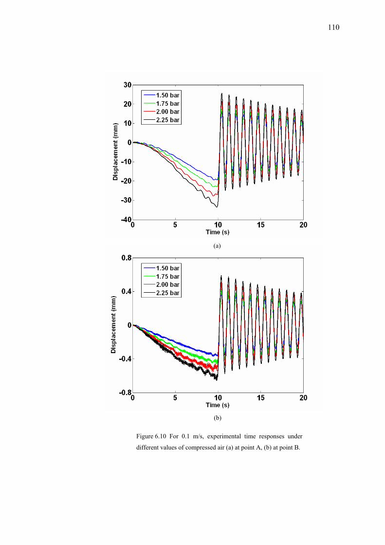
110
(a)
(b)
Figure 6.10 For 0.1 m/s, experimental time responses under
different values of compressed air (a) at point A, (b) at point B.
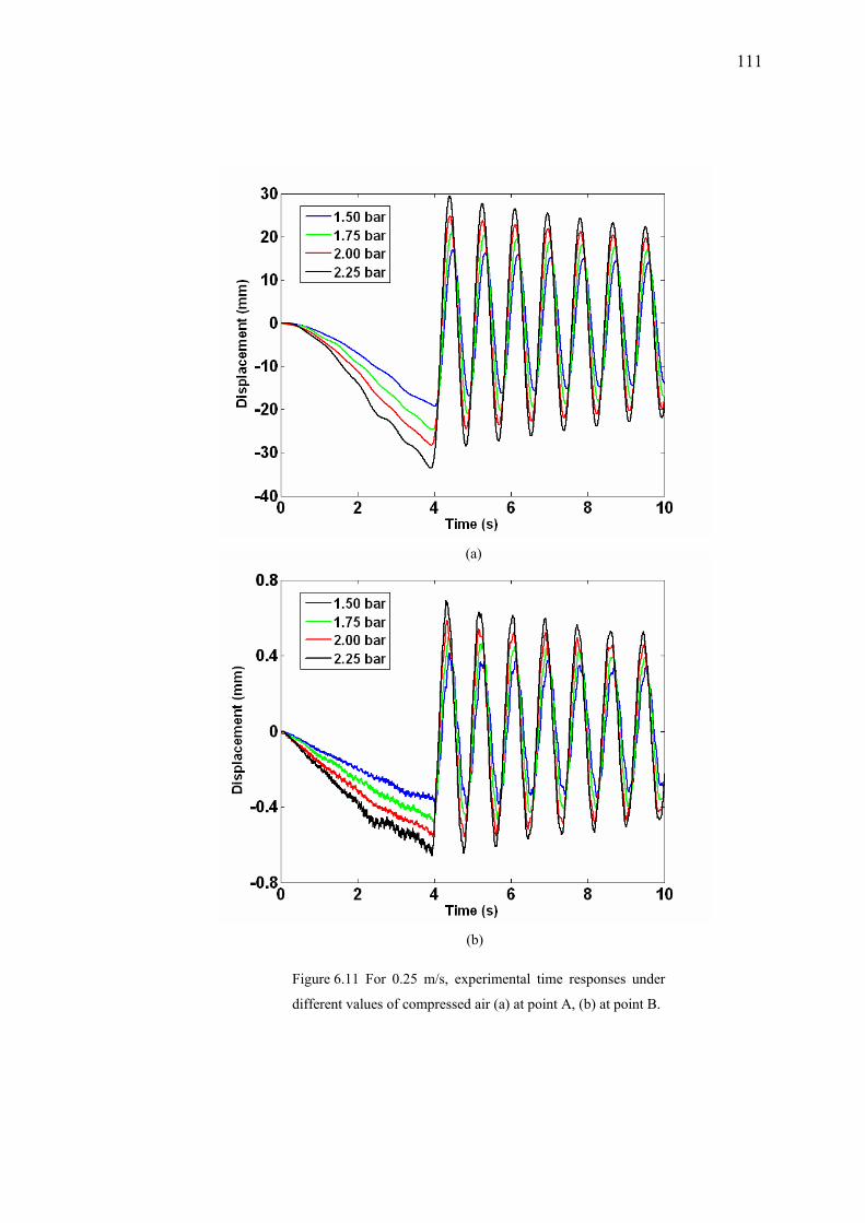
111
(a)
(b)
Figure 6.11 For 0.25 m/s, experimental time responses under
different values of compressed air (a) at point A, (b) at point B.
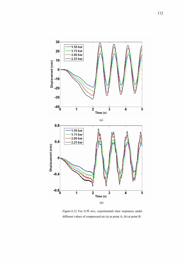
112
(a)
(b)
Figure 6.12 For 0.50 m/s, experimental time responses under
different values of compressed air (a) at point A, (b) at point B.
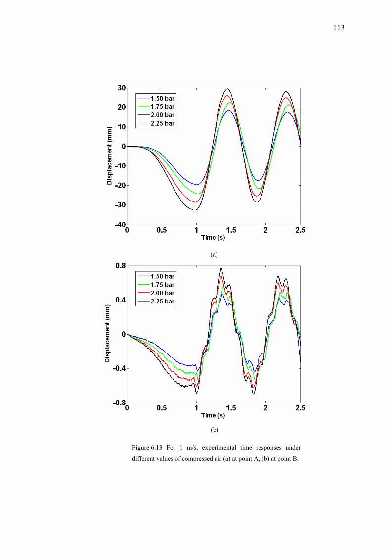
113
(a)
(b)
Figure 6.13 For 1 m/s, experimental time responses under
different values of compressed air (a) at point A, (b) at point B.
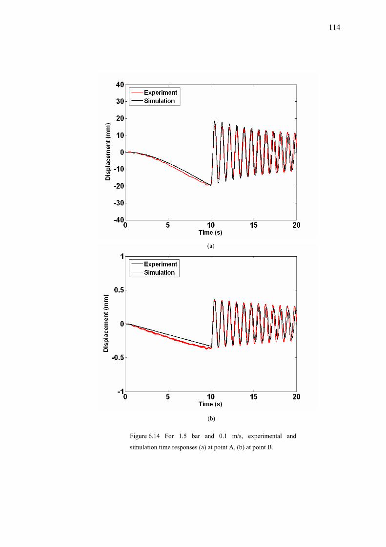
114
(a)
(b)
Figure 6.14 For 1.5 bar and 0.1 m/s, experimental and
simulation time responses (a) at point A, (b) at point B.
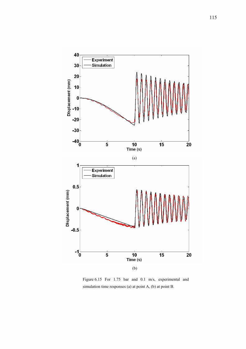
115
(a)
(b)
Figure 6.15 For 1.75 bar and 0.1 m/s, experimental and
simulation time responses (a) at point A, (b) at point B.
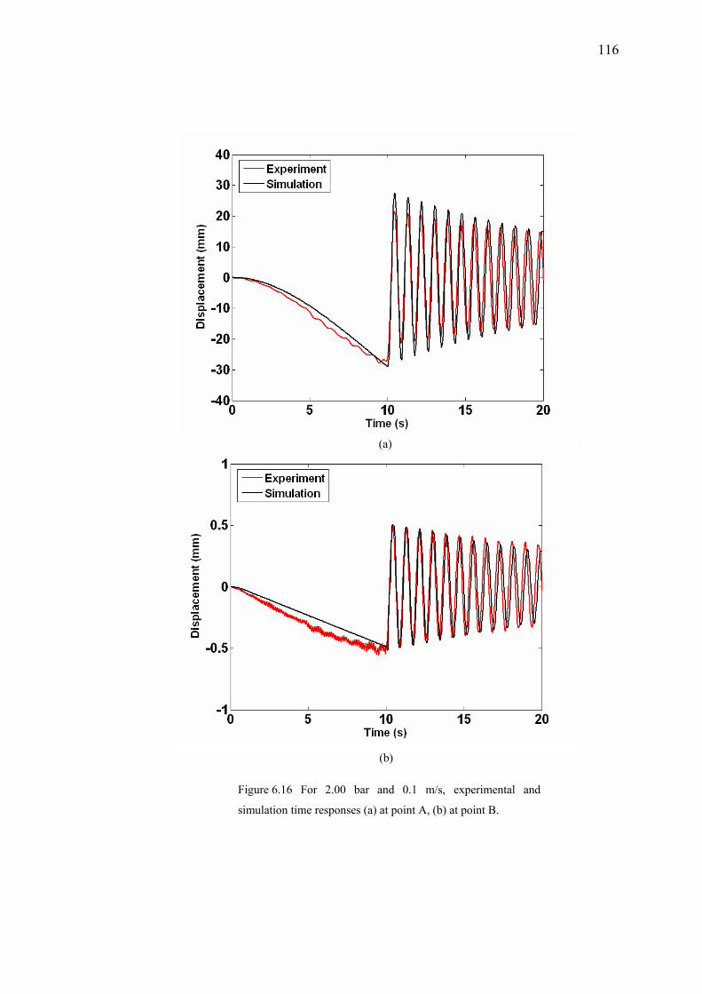
116
(a)
(b)
Figure 6.16 For 2.00 bar and 0.1 m/s, experimental and
simulation time responses (a) at point A, (b) at point B.
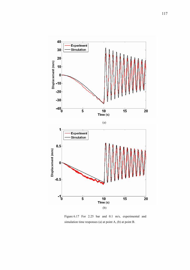
117
(a)
(b)
Figure 6.17 For 2.25 bar and 0.1 m/s, experimental and
simulation time responses (a) at point A, (b) at point B.
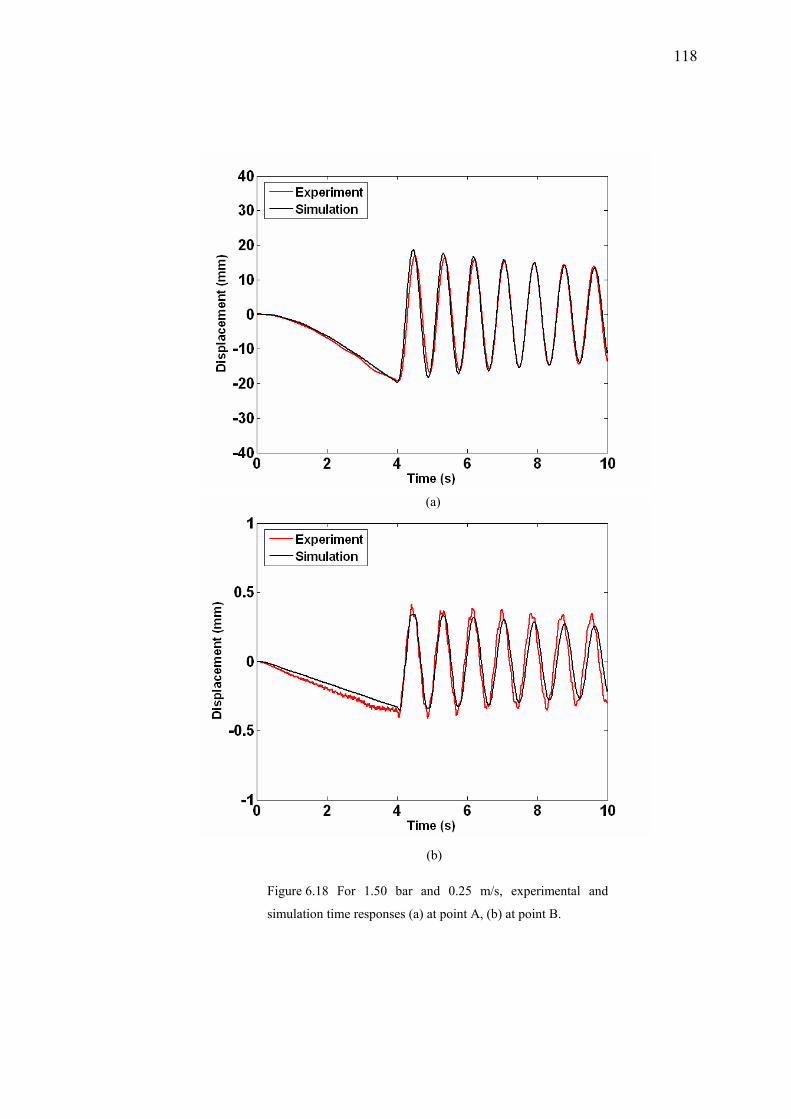
118
(a)
(b)
Figure 6.18 For 1.50 bar and 0.25 m/s, experimental and
simulation time responses (a) at point A, (b) at point B.
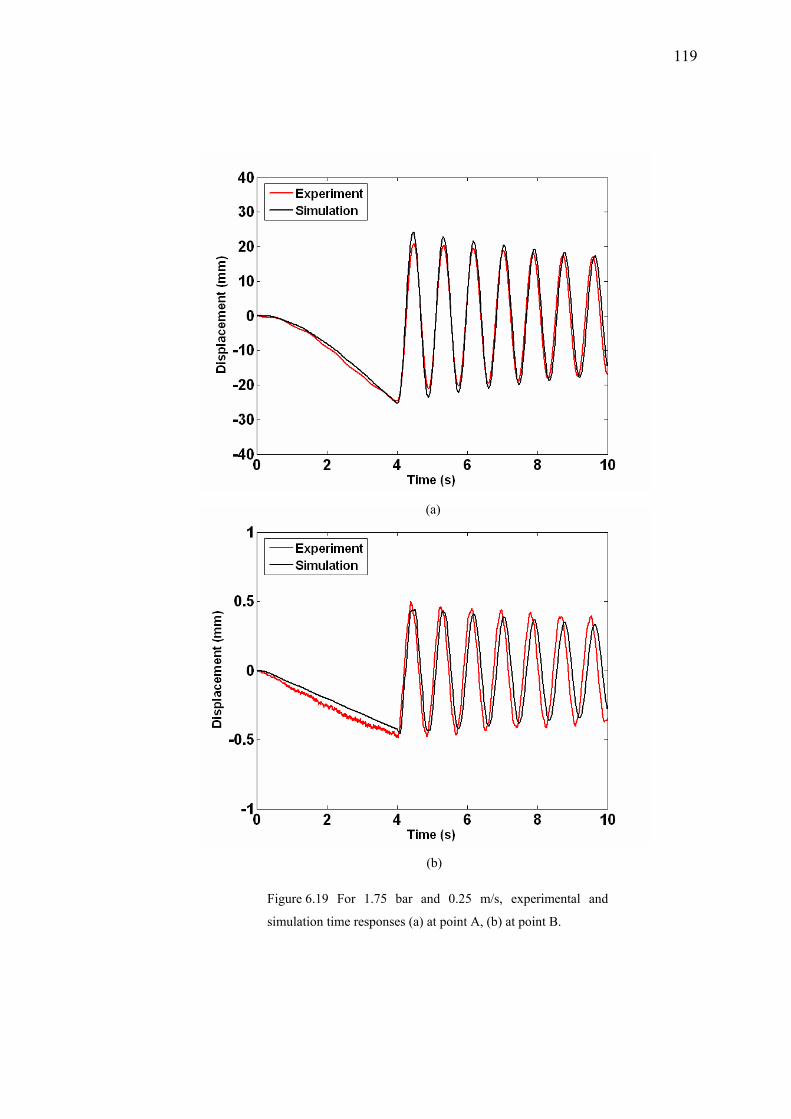
119
(a)
(b)
Figure 6.19 For 1.75 bar and 0.25 m/s, experimental and
simulation time responses (a) at point A, (b) at point B.
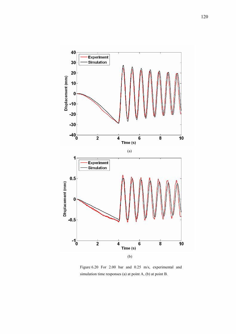
120
(a)
(b)
Figure 6.20 For 2.00 bar and 0.25 m/s, experimental and
simulation time responses (a) at point A, (b) at point B.
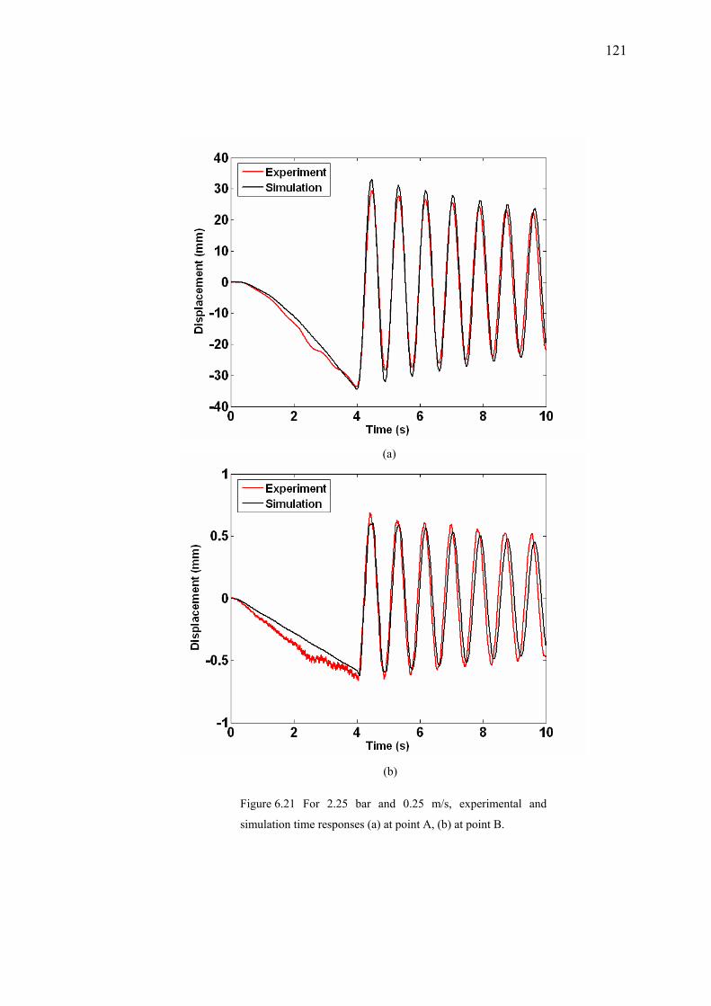
121
(a)
(b)
Figure 6.21 For 2.25 bar and 0.25 m/s, experimental and
simulation time responses (a) at point A, (b) at point B.
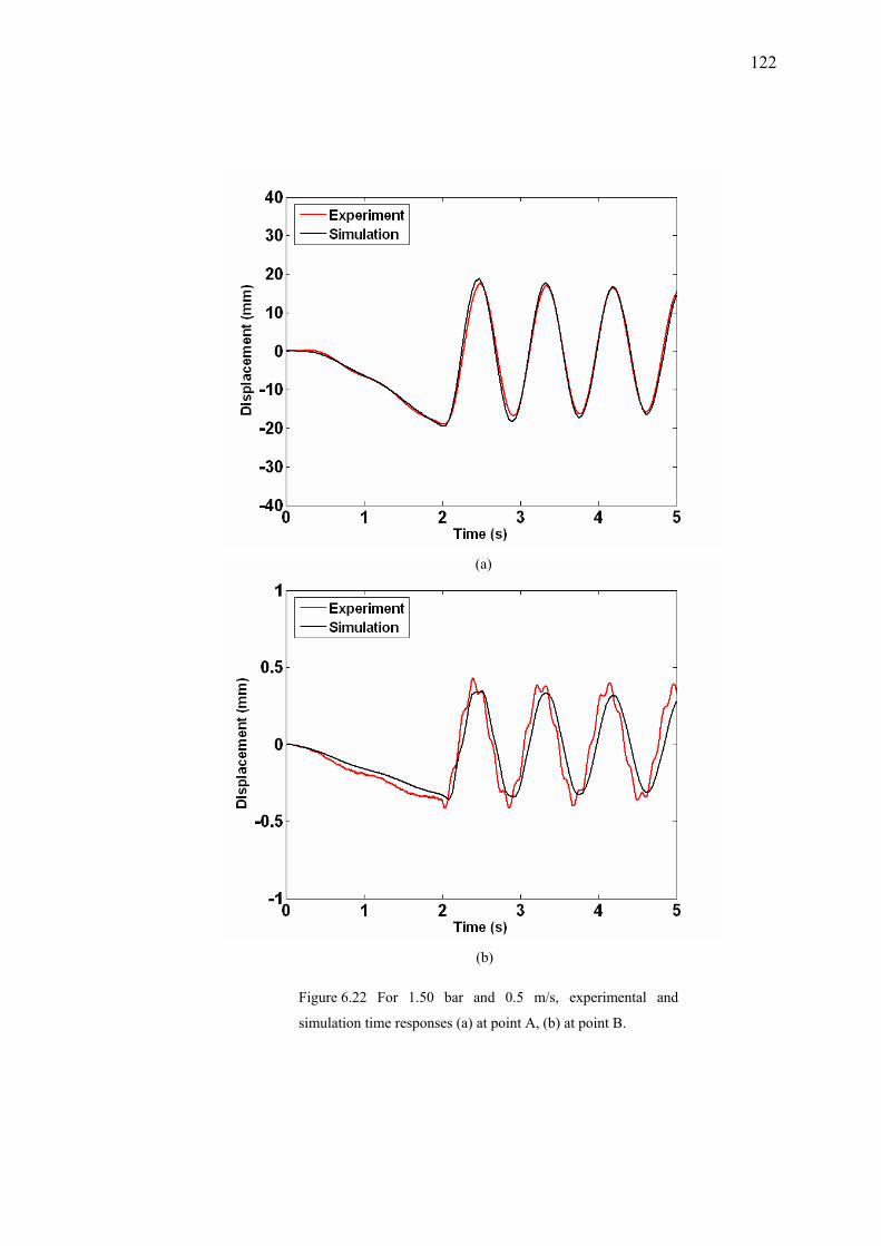
122
(a)
(b)
Figure 6.22 For 1.50 bar and 0.5 m/s, experimental and
simulation time responses (a) at point A, (b) at point B.
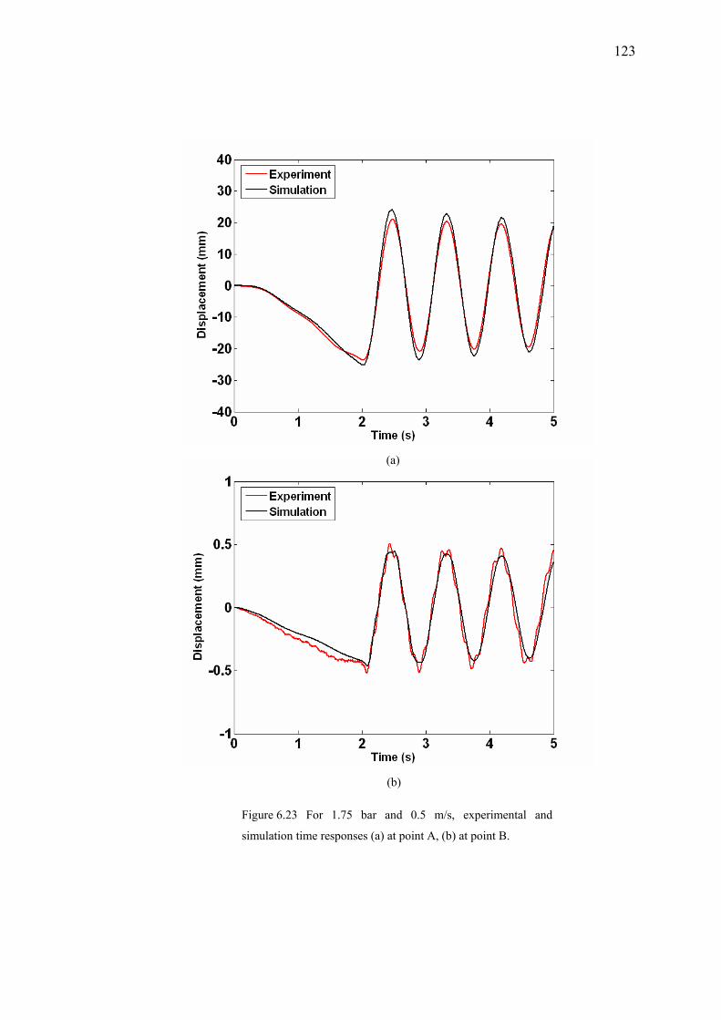
123
(a)
(b)
Figure 6.23 For 1.75 bar and 0.5 m/s, experimental and
simulation time responses (a) at point A, (b) at point B.
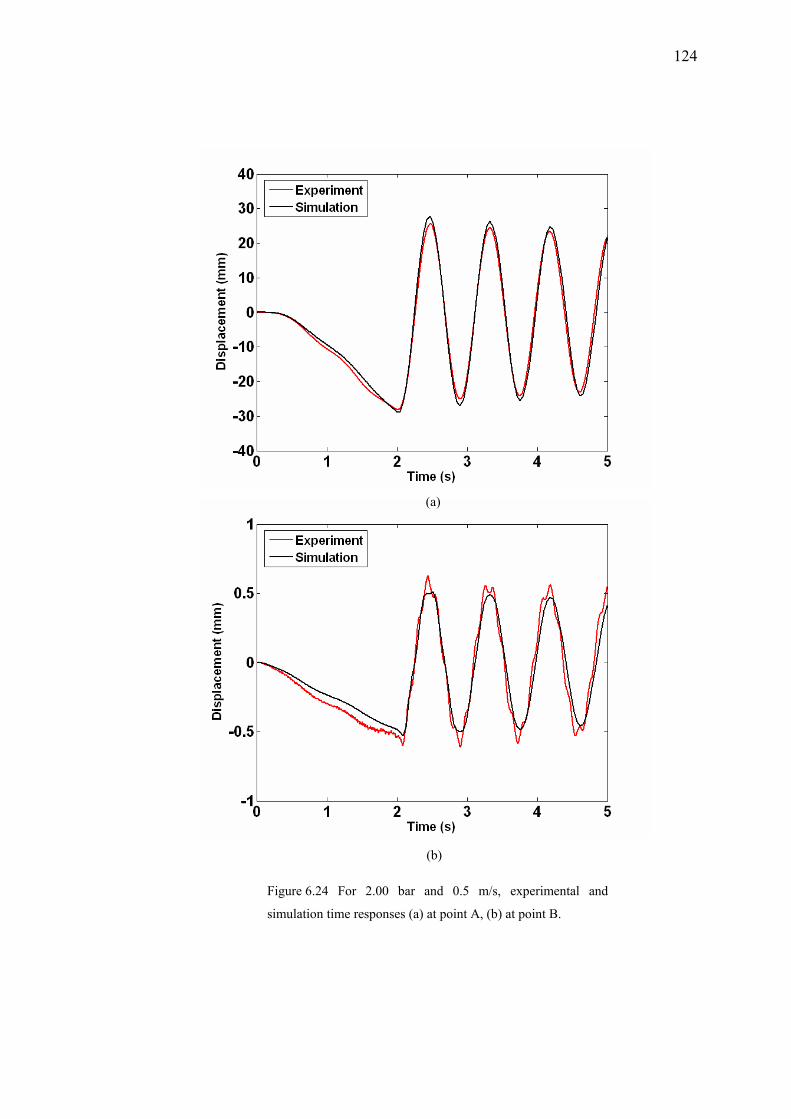
124
(a)
(b)
Figure 6.24 For 2.00 bar and 0.5 m/s, experimental and
simulation time responses (a) at point A, (b) at point B.
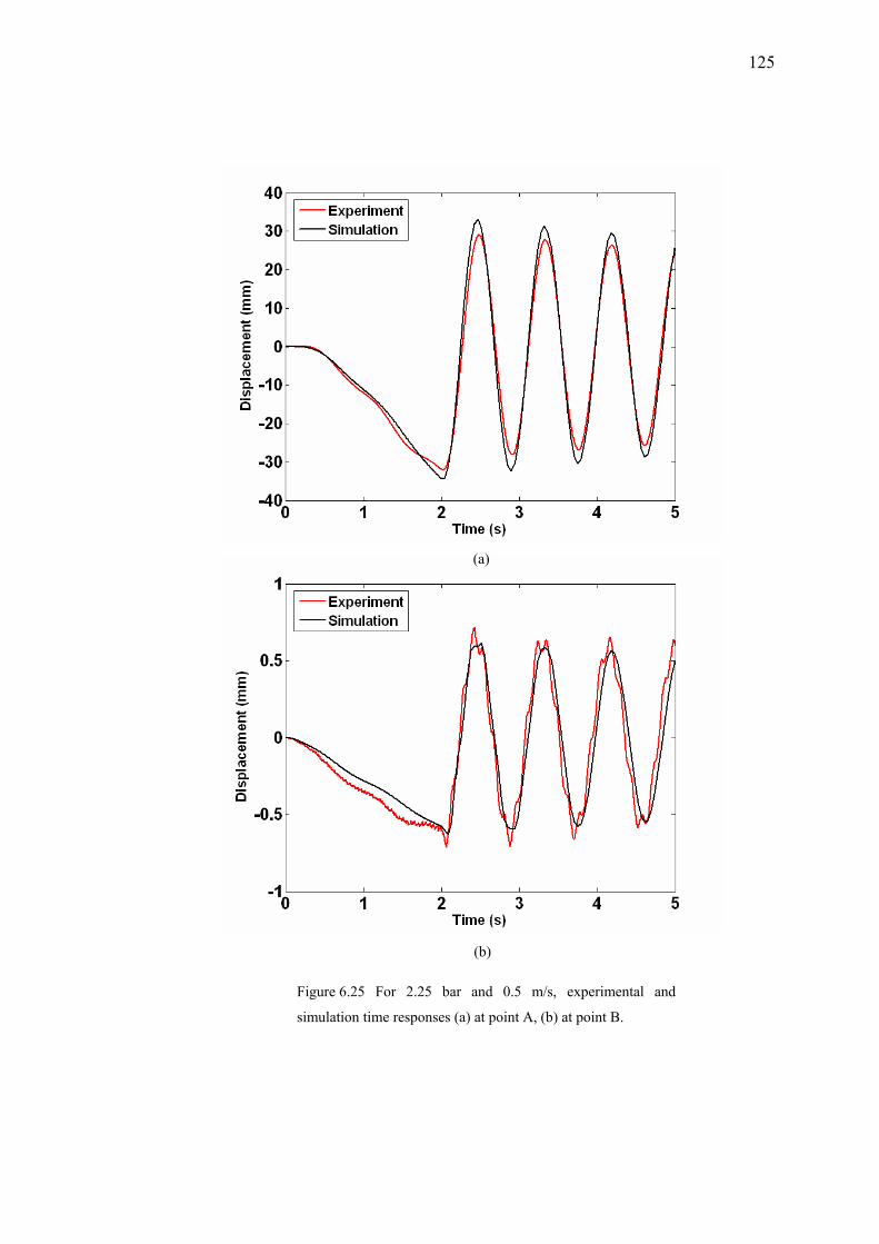
125
(a)
(b)
Figure 6.25 For 2.25 bar and 0.5 m/s, experimental and
simulation time responses (a) at point A, (b) at point B.

126
(a)
(b)
Figure 6.26 For 1.50 bar and 1 m/s, experimental and
simulation time responses (a) at point A, (b) at point B.
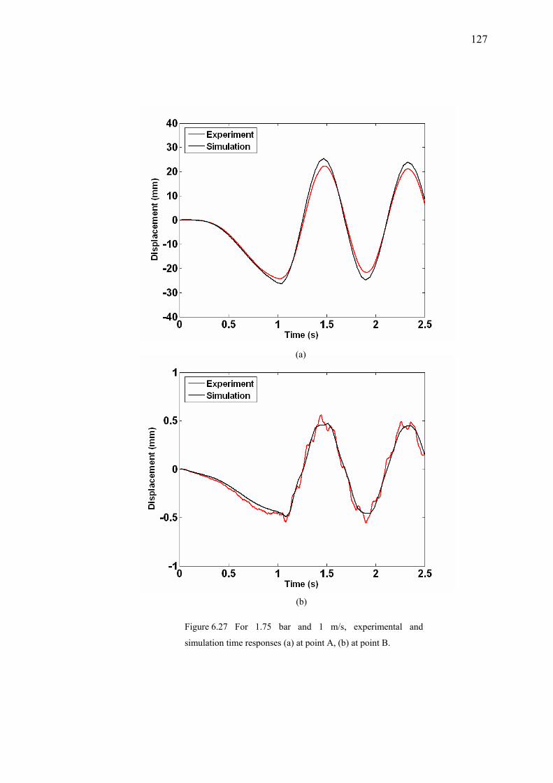
127
(a)
(b)
Figure 6.27 For 1.75 bar and 1 m/s, experimental and
simulation time responses (a) at point A, (b) at point B.
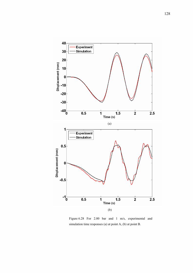
128
(a)
(b)
Figure 6.28 For 2.00 bar and 1 m/s, experimental and
simulation time responses (a) at point A, (b) at point B.
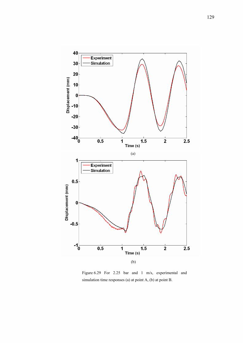
129
(a)
(b)
Figure 6.29 For 2.25 bar and 1 m/s, experimental and
simulation time responses (a) at point A, (b) at point B.
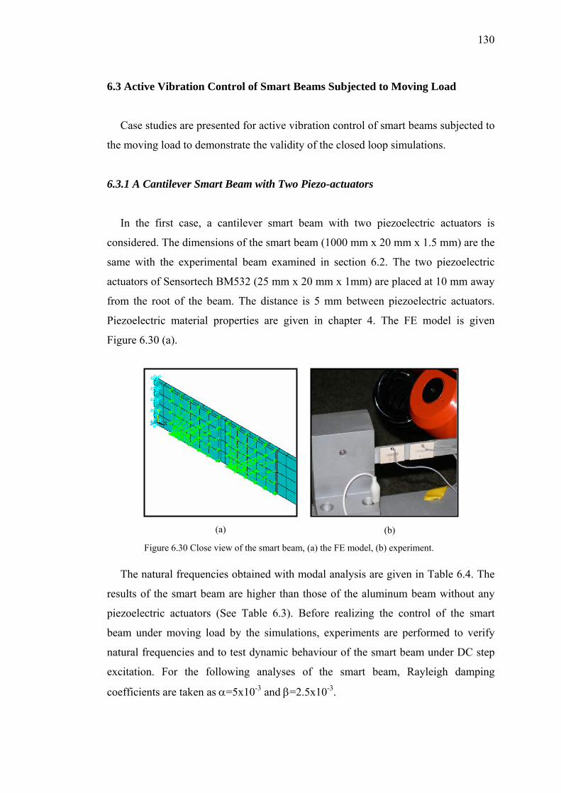
130
6.3 Active Vibration Control of Smart Beams Subjected to Moving Load
Case studies are presented for active vibration control of smart beams subjected to
the moving load to demonstrate the validity of the closed loop simulations.
6.3.1 A Cantilever Smart Beam with Two Piezo-actuators
In the first case, a cantilever smart beam with two piezoelectric actuators is
considered. The dimensions of the smart beam (1000 mm x 20 mm x 1.5 mm) are the
same with the experimental beam examined in section 6.2. The two piezoelectric
actuators of Sensortech BM532 (25 mm x 20 mm x 1mm) are placed at 10 mm away
from the root of the beam. The distance is 5 mm between piezoelectric actuators.
Piezoelectric material properties are given in chapter 4. The FE model is given
Figure 6.30 (a).
The natural frequencies obtained with modal analysis are given in Table 6.4. The
results of the smart beam are higher than those of the aluminum beam without any
piezoelectric actuators (See Table 6.3). Before realizing the control of the smart
beam under moving load by the simulations, experiments are performed to verify
natural frequencies and to test dynamic behaviour of the smart beam under DC step
excitation. For the following analyses of the smart beam, Rayleigh damping
coefficients are taken as α=5x10⁻³ and β=2.5x10⁻³.
(a) (b)
Figure 6.30 Close view of the smart beam, (a) the FE model, (b) experiment.
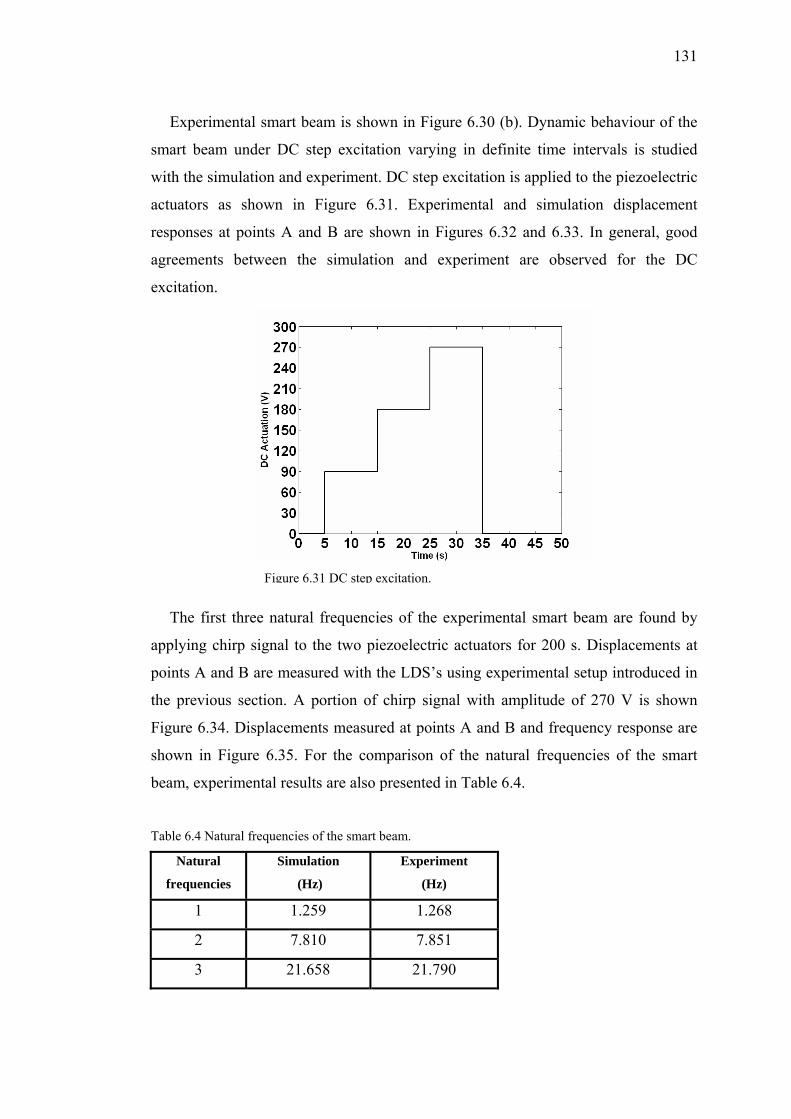
131
Experimental smart beam is shown in Figure 6.30 (b). Dynamic behaviour of the
smart beam under DC step excitation varying in definite time intervals is studied
with the simulation and experiment. DC step excitation is applied to the piezoelectric
actuators as shown in Figure 6.31. Experimental and simulation displacement
responses at points A and B are shown in Figures 6.32 and 6.33. In general, good
agreements between the simulation and experiment are observed for the DC
excitation.
The first three natural frequencies of the experimental smart beam are found by
applying chirp signal to the two piezoelectric actuators for 200 s. Displacements at
points A and B are measured with the LDS’s using experimental setup introduced in
the previous section. A portion of chirp signal with amplitude of 270 V is shown
Figure 6.34. Displacements measured at points A and B and frequency response are
shown in Figure 6.35. For the comparison of the natural frequencies of the smart
beam, experimental results are also presented in Table 6.4.
Table 6.4 Natural frequencies of the smart beam.
Natural
frequencies
Simulation
(Hz)
Experiment
(Hz)
1 1.259 1.268
2 7.810 7.851
3 21.658 21.790
Figure 6.31 DC step excitation.
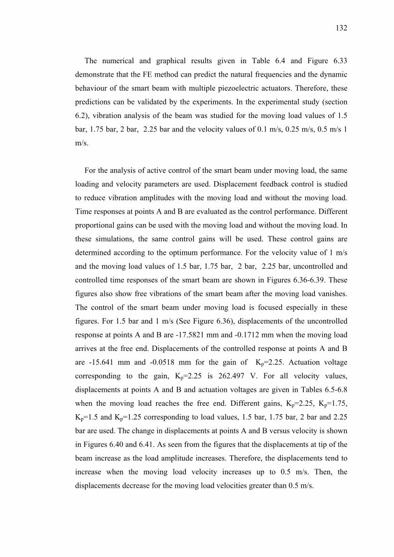
132
The numerical and graphical results given in Table 6.4 and Figure 6.33
demonstrate that the FE method can predict the natural frequencies and the dynamic
behaviour of the smart beam with multiple piezoelectric actuators. Therefore, these
predictions can be validated by the experiments. In the experimental study (section
6.2), vibration analysis of the beam was studied for the moving load values of 1.5
bar, 1.75 bar, 2 bar, 2.25 bar and the velocity values of 0.1 m/s, 0.25 m/s, 0.5 m/s 1
m/s.
For the analysis of active control of the smart beam under moving load, the same
loading and velocity parameters are used. Displacement feedback control is studied
to reduce vibration amplitudes with the moving load and without the moving load.
Time responses at points A and B are evaluated as the control performance. Different
proportional gains can be used with the moving load and without the moving load. In
these simulations, the same control gains will be used. These control gains are
determined according to the optimum performance. For the velocity value of 1 m/s
and the moving load values of 1.5 bar, 1.75 bar, 2 bar, 2.25 bar, uncontrolled and
controlled time responses of the smart beam are shown in Figures 6.36-6.39. These
figures also show free vibrations of the smart beam after the moving load vanishes.
The control of the smart beam under moving load is focused especially in these
figures. For 1.5 bar and 1 m/s (See Figure 6.36), displacements of the uncontrolled
response at points A and B are -17.5821 mm and -0.1712 mm when the moving load
arrives at the free end. Displacements of the controlled response at points A and B
are -15.641 mm and -0.0518 mm for the gain of Kp=2.25. Actuation voltage
corresponding to the gain, Kp=2.25 is 262.497 V. For all velocity values,
displacements at points A and B and actuation voltages are given in Tables 6.5-6.8
when the moving load reaches the free end. Different gains, Kp=2.25, Kp=1.75,
Kp=1.5 and Kp=1.25 corresponding to load values, 1.5 bar, 1.75 bar, 2 bar and 2.25
bar are used. The change in displacements at points A and B versus velocity is shown
in Figures 6.40 and 6.41. As seen from the figures that the displacements at tip of the
beam increase as the load amplitude increases. Therefore, the displacements tend to
increase when the moving load velocity increases up to 0.5 m/s. Then, the
displacements decrease for the moving load velocities greater than 0.5 m/s.
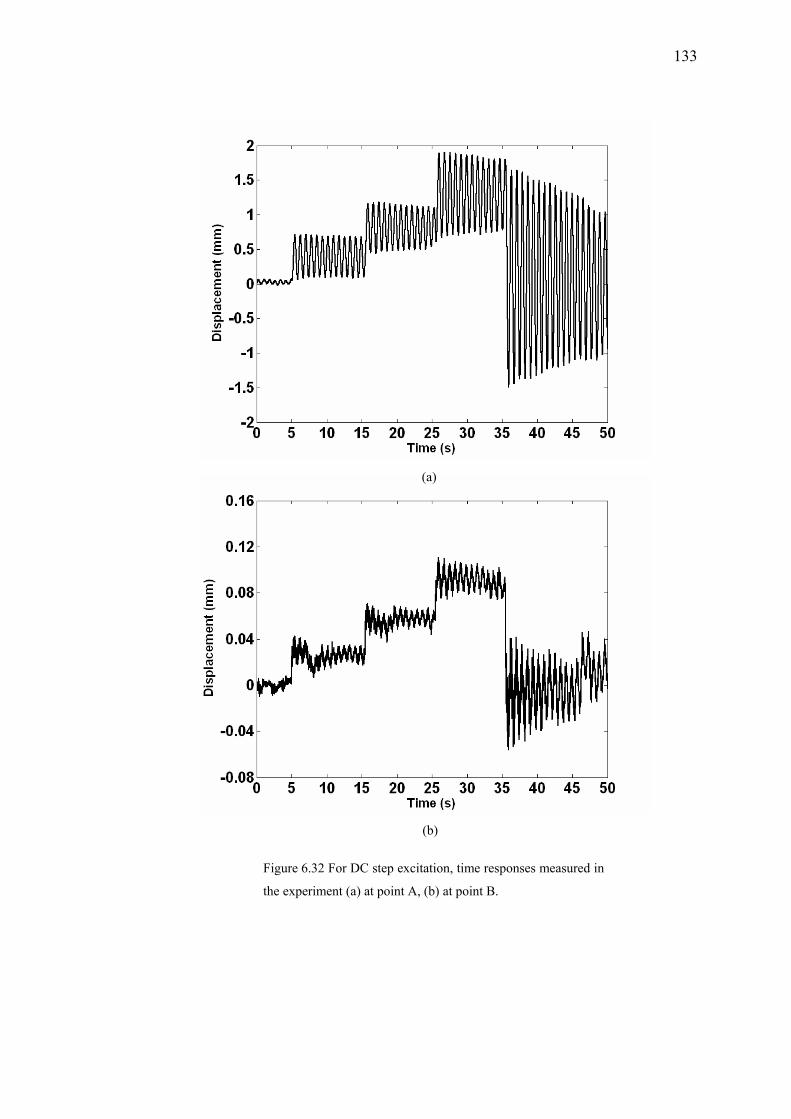
133
(a)
(b)
Figure 6.32 For DC step excitation, time responses measured in
the experiment (a) at point A, (b) at point B.
134
(a)
(b)
Figure 6.33 For DC step excitation, time responses obtained
with the simulation (a) at point A, (b) at point B.
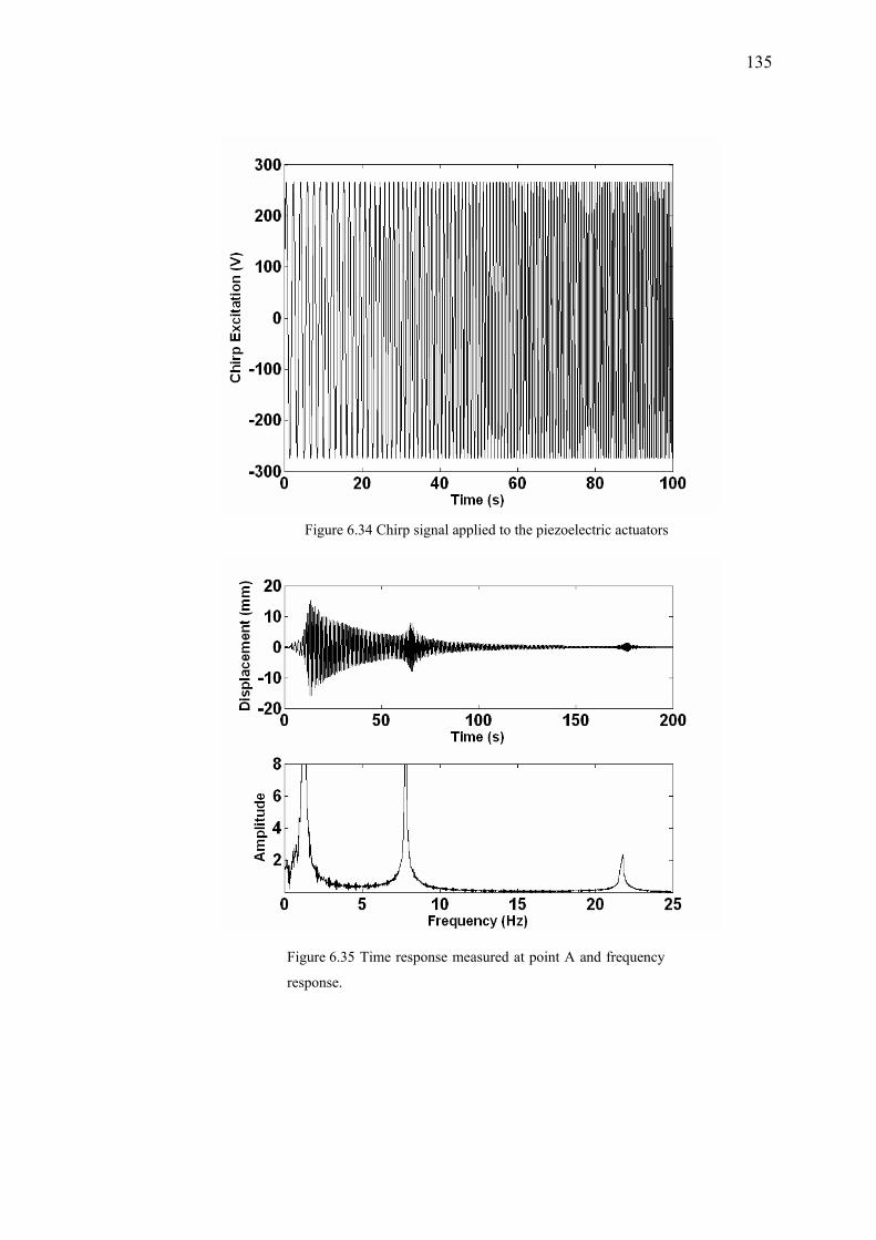
135
Figure 6.35 Time response measured at point A and frequency
response.
Figure 6.34 Chirp signal applied to the piezoelectric actuators
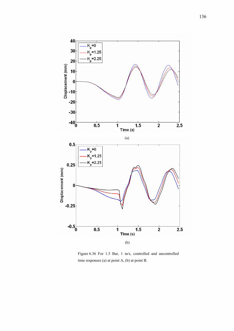
136
(a)
(b)
Figure 6.36 For 1.5 Bar, 1 m/s, controlled and uncontrolled
time responses (a) at point A, (b) at point B.
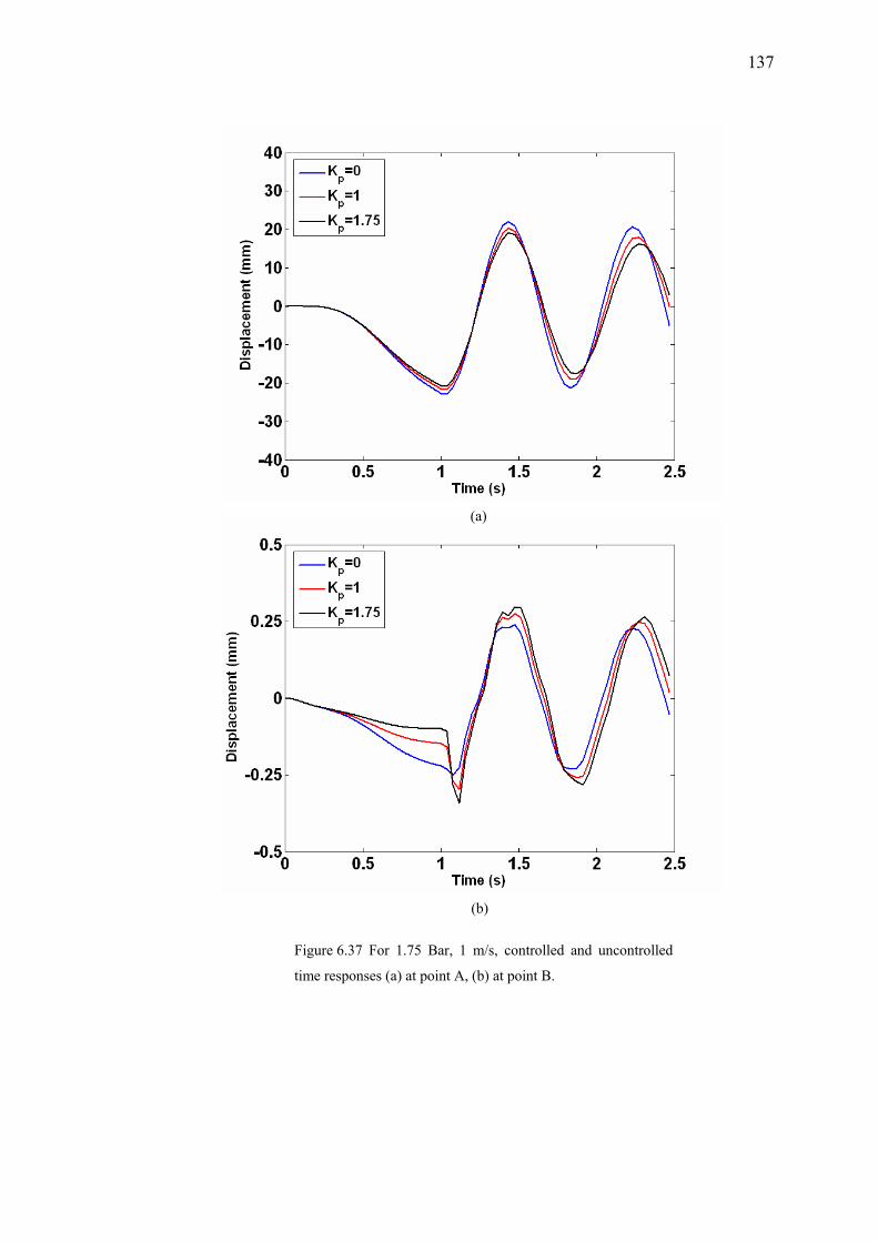
137
(a)
(b)
Figure 6.37 For 1.75 Bar, 1 m/s, controlled and uncontrolled
time responses (a) at point A, (b) at point B.
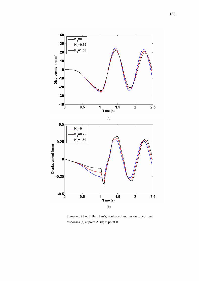
138
(a)
(b)
Figure 6.38 For 2 Bar, 1 m/s, controlled and uncontrolled time
responses (a) at point A, (b) at point B.
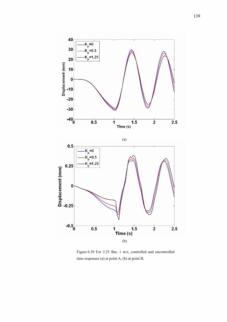
139
(a)
(b)
Figure 6.39 For 2.25 Bar, 1 m/s, controlled and uncontrolled
time responses (a) at point A, (b) at point B.
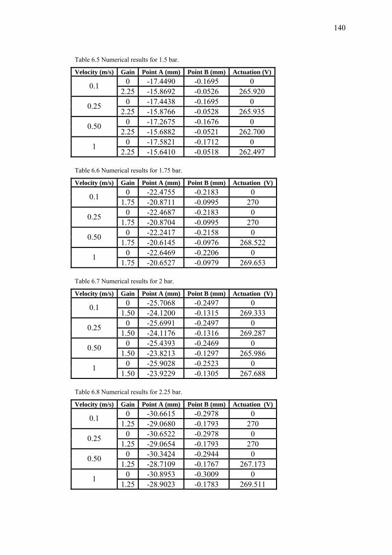
140
Table 6.5 Numerical results for 1.5 bar.
Velocity (m/s) Gain Point A (mm) Point B (mm) Actuation (V)0 -17.4490 -0.1695 0 0.1
2.25 -15.8692 -0.0526 265.920 0 -17.4438 -0.1695 0 0.25
2.25 -15.8766 -0.0528 265.935 0 -17.2675 -0.1676 0 0.50
2.25 -15.6882 -0.0521 262.700 0 -17.5821 -0.1712 0 1
2.25 -15.6410 -0.0518 262.497 Table 6.6 Numerical results for 1.75 bar.
Velocity (m/s) Gain Point A (mm) Point B (mm) Actuation (V)0 -22.4755 -0.2183 0 0.1
1.75 -20.8711 -0.0995 270 0 -22.4687 -0.2183 0 0.25
1.75 -20.8704 -0.0995 270 0 -22.2417 -0.2158 0 0.50
1.75 -20.6145 -0.0976 268.522 0 -22.6469 -0.2206 0 1
1.75 -20.6527 -0.0979 269.653 Table 6.7 Numerical results for 2 bar.
Velocity (m/s) Gain Point A (mm) Point B (mm) Actuation (V)0 -25.7068 -0.2497 0 0.1
1.50 -24.1200 -0.1315 269.333 0 -25.6991 -0.2497 0 0.25
1.50 -24.1176 -0.1316 269.287 0 -25.4393 -0.2469 0 0.50
1.50 -23.8213 -0.1297 265.986 0 -25.9028 -0.2523 0 1
1.50 -23.9229 -0.1305 267.688 Table 6.8 Numerical results for 2.25 bar.
Velocity (m/s) Gain Point A (mm) Point B (mm) Actuation (V)0 -30.6615 -0.2978 0 0.1
1.25 -29.0680 -0.1793 270 0 -30.6522 -0.2978 0 0.25
1.25 -29.0654 -0.1793 270 0 -30.3424 -0.2944 0 0.50
1.25 -28.7109 -0.1767 267.173 0 -30.8953 -0.3009 0 1
1.25 -28.9023 -0.1783 269.511
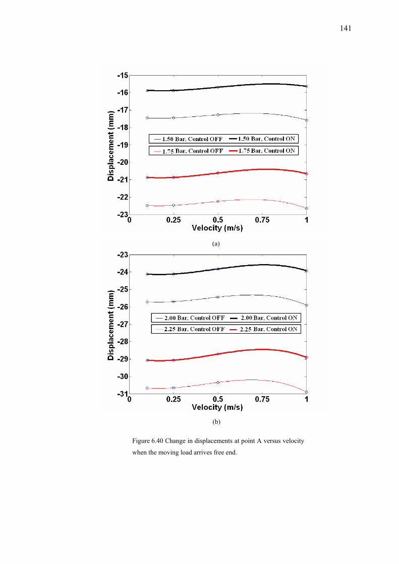
141
(a)
(b)
Figure 6.40 Change in displacements at point A versus velocity
when the moving load arrives free end.
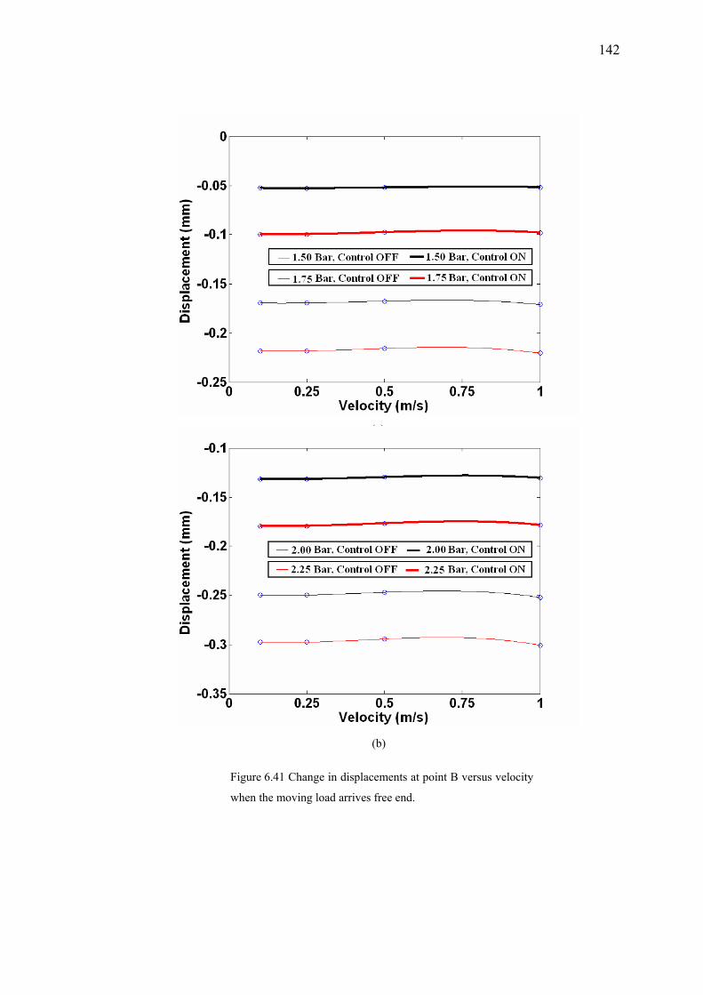
142
(a)
(b)
Figure 6.41 Change in displacements at point B versus velocity
when the moving load arrives free end.
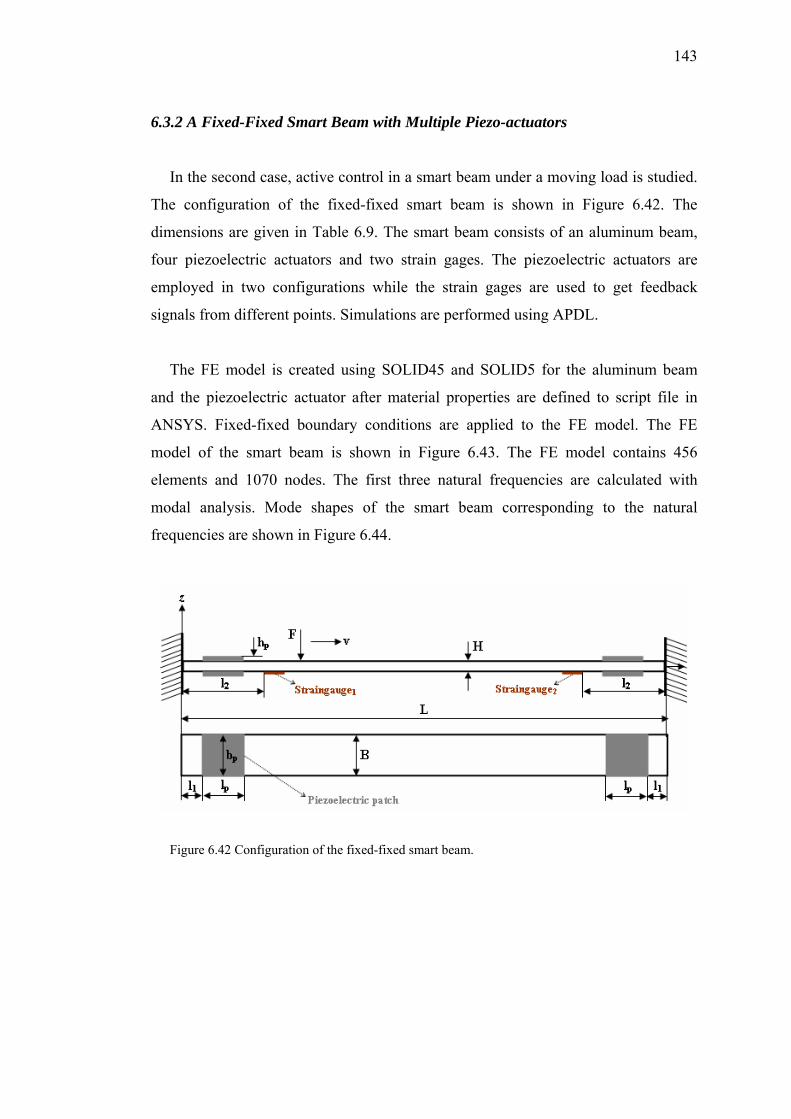
143
6.3.2 A Fixed-Fixed Smart Beam with Multiple Piezo-actuators
In the second case, active control in a smart beam under a moving load is studied.
The configuration of the fixed-fixed smart beam is shown in Figure 6.42. The
dimensions are given in Table 6.9. The smart beam consists of an aluminum beam,
four piezoelectric actuators and two strain gages. The piezoelectric actuators are
employed in two configurations while the strain gages are used to get feedback
signals from different points. Simulations are performed using APDL.
The FE model is created using SOLID45 and SOLID5 for the aluminum beam
and the piezoelectric actuator after material properties are defined to script file in
ANSYS. Fixed-fixed boundary conditions are applied to the FE model. The FE
model of the smart beam is shown in Figure 6.43. The FE model contains 456
elements and 1070 nodes. The first three natural frequencies are calculated with
modal analysis. Mode shapes of the smart beam corresponding to the natural
frequencies are shown in Figure 6.44.
Figure 6.42 Configuration of the fixed-fixed smart beam.
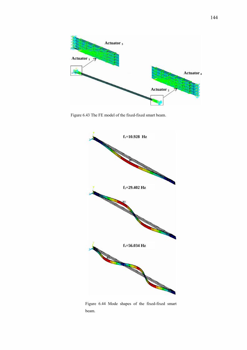
144
Actuator 1
Actuator 2
Actuator 3
Actuator 4
f1=10.928 Hz
f2=29.402 Hz
f3=56.034 Hz
Figure 6.43 The FE model of the fixed-fixed smart beam.
Figure 6.44 Mode shapes of the fixed-fixed smart
beam.
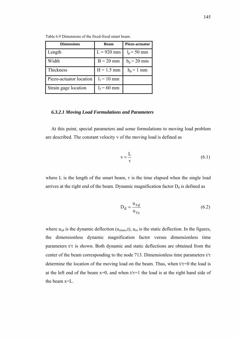
145
Table 6.9 Dimensions of the fixed-fixed smart beam.
Dimensions Beam Piezo-actuator
Length L = 920 mm lp = 50 mm
Width B = 20 mm bp = 20 mm
Thickness H = 1.5 mm hp = 1 mm
Piezo-actuator location l1 = 10 mm
Strain gage location l2 = 60 mm
6.3.2.1 Moving Load Formulations and Parameters
At this point, special parameters and some formulations to moving load problem
are described. The constant velocity v of the moving load is defined as
τ=
Lv (6.1)
where L is the length of the smart beam, τ is the time elapsed when the single load
arrives at the right end of the beam. Dynamic magnification factor Dd is defined as
sz
dzd u
uD = (6.2)
where uzd is the dynamic deflection (uzmax,t), uzs is the static deflection. In the figures,
the dimensionless dynamic magnification factor versus dimensionless time
parameters t/τ is shown. Both dynamic and static deflections are obtained from the
center of the beam corresponding to the node 713. Dimensionless time parameters t/τ
determine the location of the moving load on the beam. Thus, when t/τ=0 the load is
at the left end of the beam x=0, and when t/τ=1 the load is at the right hand side of
the beam x=L.
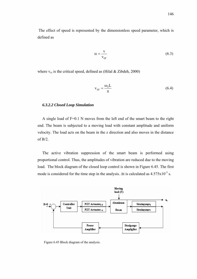
146
The effect of speed is represented by the dimensionless speed parameter, which is
defined as
crvv
=α (6.3)
where vcr is the critical speed, defined as (Hilal & Zibdeh, 2000)
πω
=L
v 1cr (6.4)
6.3.2.2 Closed Loop Simulation
A single load of F=0.1 N moves from the left end of the smart beam to the right
end. The beam is subjected to a moving load with constant amplitude and uniform
velocity. The load acts on the beam in the z direction and also moves in the distance
of B/2.
The active vibration suppression of the smart beam is performed using
proportional control. Thus, the amplitudes of vibration are reduced due to the moving
load. The block diagram of the closed loop control is shown in Figure 6.45. The first
mode is considered for the time step in the analysis. Δt is calculated as 4.575x10⁻³ s.
Figure 6.45 Block diagram of the analysis.
147
The feedback signals are obtained from the two strain gages (strain gage1 and
strain gage2). The two strain gages which sense the feedback signals at different
locations are utilized to calculate the actuation voltages. The gains for the strain gage
and power amplifier are taken as 10000 and 30 in the analysis, respectively.
Two configurations are studied to demonstrate the effectiveness of the active
control. Four actuators are employed as the following;
• Monomorph configuration; Actuator1 (Act1) and Actuator2 (Act2) are active
Actuator3 (Act3) and Actuator4 (Act4) are passive.
• Bimorph configuration; All actuators are active. Act1-Act3 work together as
coupled actuators as well as Act2-Act4.
In monomorph configuration, actuation voltages are applied to the actuators Act1
and Act2. In bimorph configuration, actuation voltages are applied to a group of
actuators; Act1-Act3 and Act2-Act4 at the same time. Results are obtained for the
speed parameter α (1, 0.5 and 0.25) and for various control gains. In the simulations,
Rayleigh damping coefficients are taken as αd = βd = 0.0005.
The difference of monomorph and bimorph configurations is presented with the
following figures. The results, in Figures from 6.46 to 6.51 are obtained for all values
of α when the gains are equal, Kp1=Kp2. Figures 6.46 (monomorph configuration)
and 6.49 (bimorph configuration) show dimensionless dynamic magnification factor
versus dimensionless time ratios for α=1, α=0.5, α=0.25, respectively. The vibration
amplitudes due to the moving load are reduced with active control as the controller
gain increases. The form of the figures is different since the velocity of the moving
load changes. Better reductions are provided with bimorph configuration as shown in
Figure 6.48. For a low speed parameter (α=0.25) the dynamic deflection under the
moving load is smaller than the static deflection in bimorph configuration.
148
For monomorph configuration, actuation voltages applied to Act1 and Act2 versus
motion time of the load are shown in Figures 6.47 and 6.48. For bimorph
configuration, actuation voltages applied to Act1-Act3 and Act2-Act4 versus motion
time of the load are shown in Figures 6.50 and 6.51. It is noticed that the actuation
voltages increase as the controller gain increases. The forms of the actuation voltages
are different since the feedback is provided from the two strain gages at different
locations. The vibration amplitudes can be reduced more effectively applying
approximately same actuation voltage levels with bimorph configuration.
When different voltages are applied to the group of actuators Kp2 =3/2Kp1,
dynamic magnification factor and actuation voltages for α=1, and bimorph
configuration are shown in Figure 6.52. A larger reduction is provided for higher
controller gains in the dynamic magnification factor as shown in Figure 6.52 (a).
Actuation voltage applied to Act1-Act3 and Act2-Act4 are shown in Figures 6.52 (b)
and 6.52 (c), respectively. It is possible to increase the controller gains if different
voltages are applied to the group of actuators.
149
(a)
(b)
(c)
Figure 6.46 Kp2=Kp1, dynamic magnification
factor versus dimensionless time parameter,
a) α=1, (b) α=0.5, (c) α=0.25.
Monomorph Configuration
Monomorph Configuration
Monomorph Configuration
150
(a)
(b)
(c)
Figure 6.47 Kp2=Kp1, actuator voltages applied to
Act1, a) α=1, (b) α=0.5, (c) α=0.25.
Monomorph Configuration
Monomorph Configuration
Monomorph Configuration
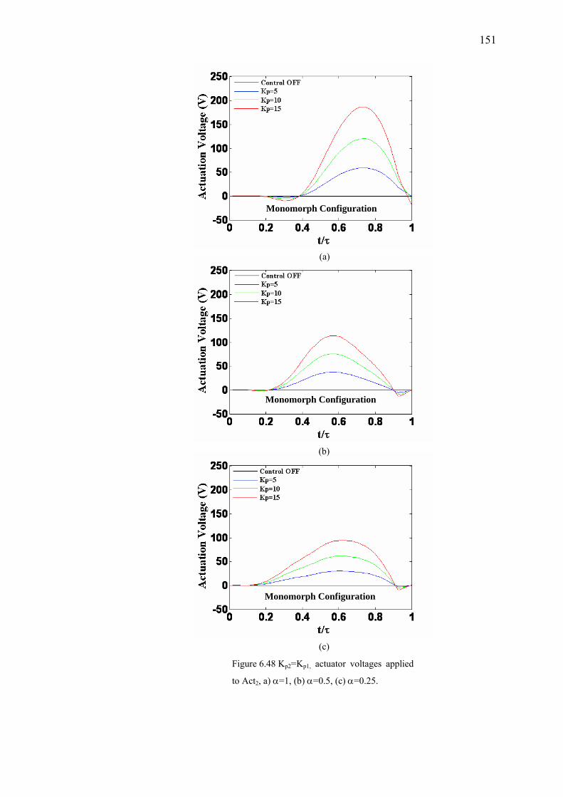
151
(a)
(b)
(c)
Figure 6.48 Kp2=Kp1, actuator voltages applied
to Act2, a) α=1, (b) α=0.5, (c) α=0.25.
Monomorph Configuration
Monomorph Configuration
Monomorph Configuration
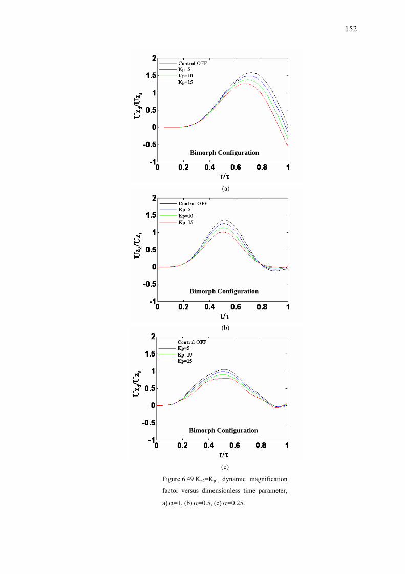
152
(a)
(b)
(c)
Figure 6.49 Kp2=Kp1, dynamic magnification
factor versus dimensionless time parameter,
a) α=1, (b) α=0.5, (c) α=0.25.
Bimorph Configuration
Bimorph Configuration
Bimorph Configuration
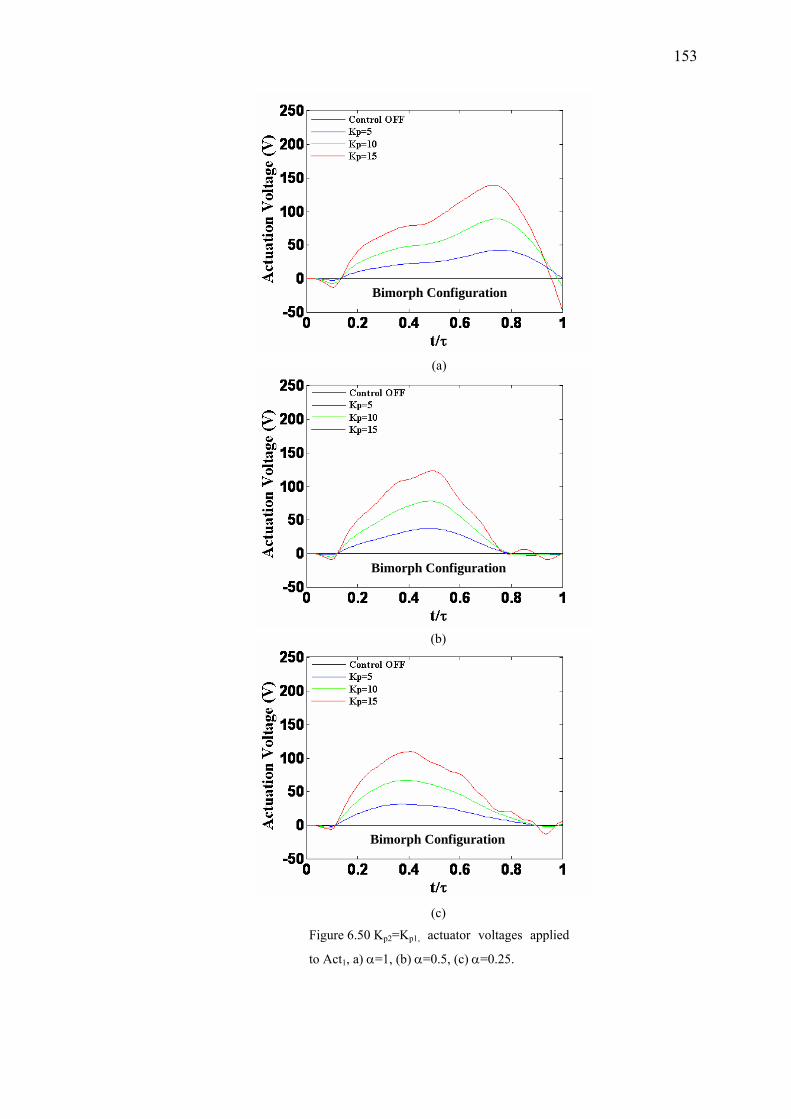
153
(a)
(b)
(c)
Figure 6.50 Kp2=Kp1, actuator voltages applied
to Act1, a) α=1, (b) α=0.5, (c) α=0.25.
Bimorph Configuration
Bimorph Configuration
Bimorph Configuration
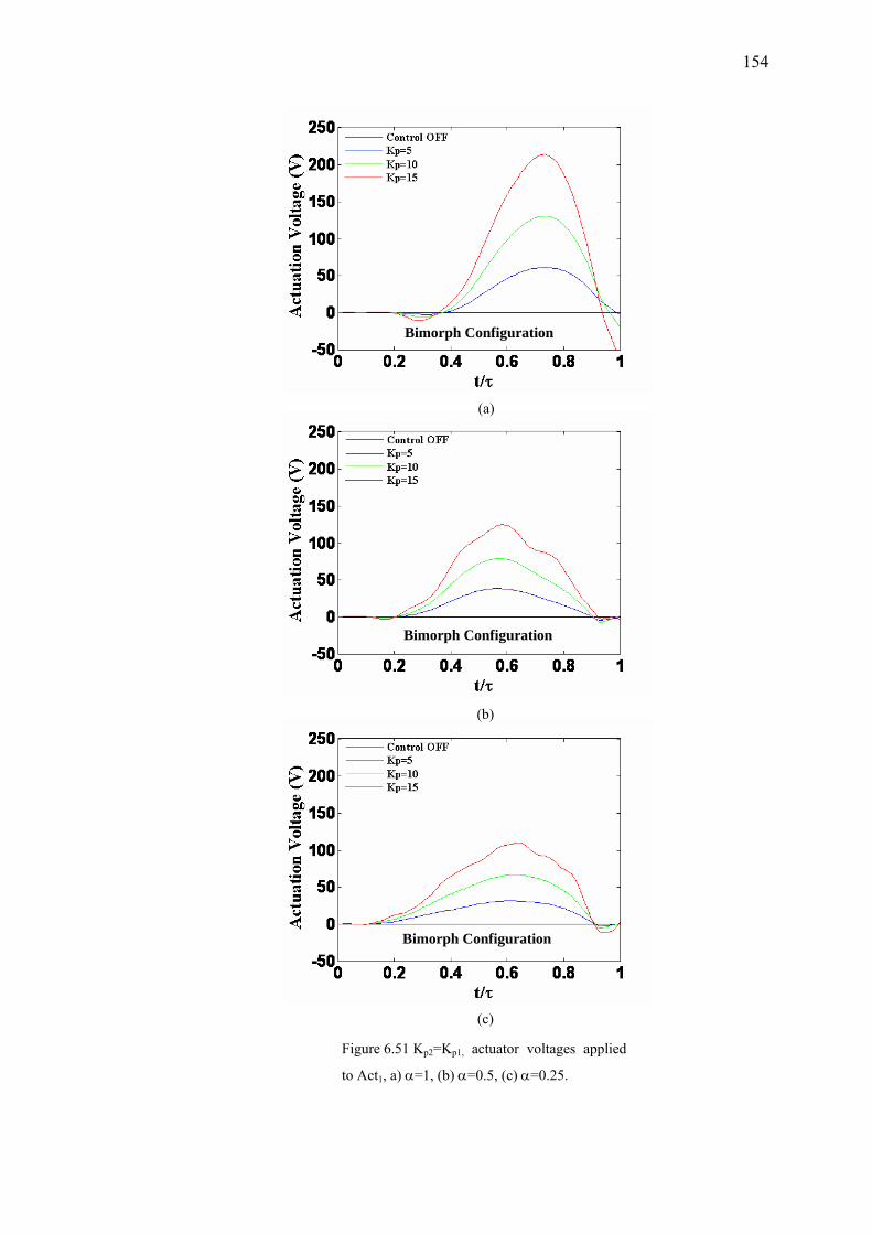
154
(a)
(b)
(c)
Bimorph Configuration
Bimorph Configuration
Bimorph Configuration
Figure 6.51 Kp2=Kp1, actuator voltages applied
to Act1, a) α=1, (b) α=0.5, (c) α=0.25.
155
(a)
(b)
(c)
Figure 6.52 α=1, Kp2 =3/2Kp1, bimorph
configuration (a) dynamic magnification
factor versus dimensionless time parameter,
(b) actuation voltage in Act1, (c) actuation
voltage in Act2.
156
CHAPTER SEVEN
RESULTS AND DISCUSSIONS
In this thesis, the active vibration control of a 3-DOF mass-spring system is
considered first. The open-loop model of the system is obtained by using Lagrange’s
equation. The Runge-Kutta method is used to solve the equations step by step. The
instantaneous value of the error signal at a time step is obtained by subtracting the
instantaneous value of the output from the instantaneous value of the reference input.
The reference input is zero for the vibration suppression. The error signal value is
processed for the control action and the input value for the subsequent step is
determined. The calculation is continued step by step until the steady-state value is
reached. The results obtained by this numerical method are compared with the results
obtained by the analytical methods using Laplace transform method. It is observed
that the results are in good agreement.
ANSYS allows defining inputs and getting outputs at a time step. Similar to the
numerical procedure described above, the closed loop analysis is performed step by
step using APDL in a loop until the steady-state value is obtained. ANSYS results
match well with the Runge-Kutta and analytical results for the 3-DOF system.
After developing and testing integration of closed loop action into FE analysis,
active vibration control of smart beams studied experimentally in the literature is
considered. Smart aluminum beams with piezoelectric actuators are modeled in
ANSYS by using SOLID45 and SOLID5 elements for metal and, piezoelectric parts,
respectively. The procedure developed has been applied successfully for smart
beams. Simulation results have also been given for the active vibration control of
smart circular discs and smart square plates. The circular plate problem is axially
symmetric. Smart plate consists of five piezoelectric actuators and sensors.
157
Experiments have been conducted to verify the simulation procedure. Aluminum
beams of 450 mm x 20 mm x 1.5 mm with piezoelectric patches of 25 mm x 20 mm
x 1 mm are considered in the experiments. The piezoelectric-material is BM532 of
Sensor Technology Company. Modal analyses, control of free and forced vibration
analyses are carried out. Experimental results are achieved by using National
Instruments products and LabVIEW. Strain and displacement feedbacks are studied.
Laser displacement sensors are used for the displacement feedback. Experimental
and ANSYS simulation results are in good agreement for uncontrolled and controlled
cases with various gain values.
Modal analyses are performed using chirp signals. The natural frequencies are
found in the frequency domain by taking the FFT of the time responses. The first two
natural frequencies of the smart beam analyzed in free vibration control are found by
changing the frequency from 0.1 Hz to 50 Hz. The first three natural frequencies of
the smart beam analyzed in forced vibration control are found by changing the
frequency from 0.1 Hz to 110 Hz. The natural frequencies obtained by the simulation
are higher than those obtained by the experiments. Perfect boundary and
electromechanical coupling conditions are assumed in the FE method. These
conditions may not be provided in the experiments perfectly.
In free vibration control, the controller gains of 5, 7, and 9 are used in case of
strain feedback while the controller gains of 1, 1.5, and 2 are used in case of
displacement feedback. Strain and displacement feedback gains are different since
the sensor gains Ks are not the same. These gains are selected to provide optimum
control performance. RMS values of time responses can be evaluated as the control
performance. In the numerical simulations, the RMS value of the uncontrolled
response is calculated as 7.99 mm. The RMS values of the controlled responses are
calculated as 6.77 mm, 6.27 mm and 5.81 mm corresponding to the gains 5, 7 and 9.
The RMS values of the controlled responses are calculated as 6.99 mm, 6.50 mm and
6.18 mm corresponding to the gains 1, 1.5 and 2. The results show that the energy of
the controlled responses is smaller than that of uncontrolled response for higher
gains. Better vibration suppressions are achieved for Kp = 9 in strain feedback and
158
Kp = 2 in displacement feedback. The maximum amplitudes of the corresponding
actuation voltages exceed 270 V for a short time interval. Saturation is applied to the
controller output for 270 V. Similar results are found in the experiments. In the
experiments, the RMS value of the uncontrolled response is found as 7.32 mm. The
RMS values of the controlled responses are found as 6.12 mm, 6.09 mm and 5.33
mm corresponding to the gains 5, 7 and 9. The RMS values of the controlled
responses are found as 6.22 mm, 5.6 mm and 5.27 mm corresponding to the gains 1,
1.5 and 2. It is observed that better control is provided for higher gains. The
amplitudes and the settling time decrease as the controller gain increases.
In forced vibration control, results are obtained for the gains of 3.75, 7.5 and 15.
For Kp = 15, the maximum actuation voltages in the strain and displacement feedback
controls are 50 V and 95 V, respectively. In numerical simulations, strain and
displacement feedback control provides 63 % and 87 % reduction in steady-state
vibration amplitudes. Simulation results show that the displacement feedback control
is more effective since it enables to apply higher actuation voltages for the values of
the same gain. Similar to, experimental results show that strain and displacement
controls provide 61.5 % and 85 % reduction in the steady-state amplitudes. It is
observed that experimental and simulation results are in good agreement.
Finally beams under moving load have been analyzed. Vibration analyses of a
cantilever aluminum beam of 1000 mm x 20 mm x 1.5 mm are performed by the
experiments and simulations. The moving load is provided by using a six axes
industrial robot IRB 1400 of ABB. The load is produced with air blower nozzle
attached to the last arm of the robot. Good results are observed between the
experiments and the simulations for various speed and load values. Simulation
results using the procedure developed in this thesis have been given for the active
vibration control of smart beams under moving load.
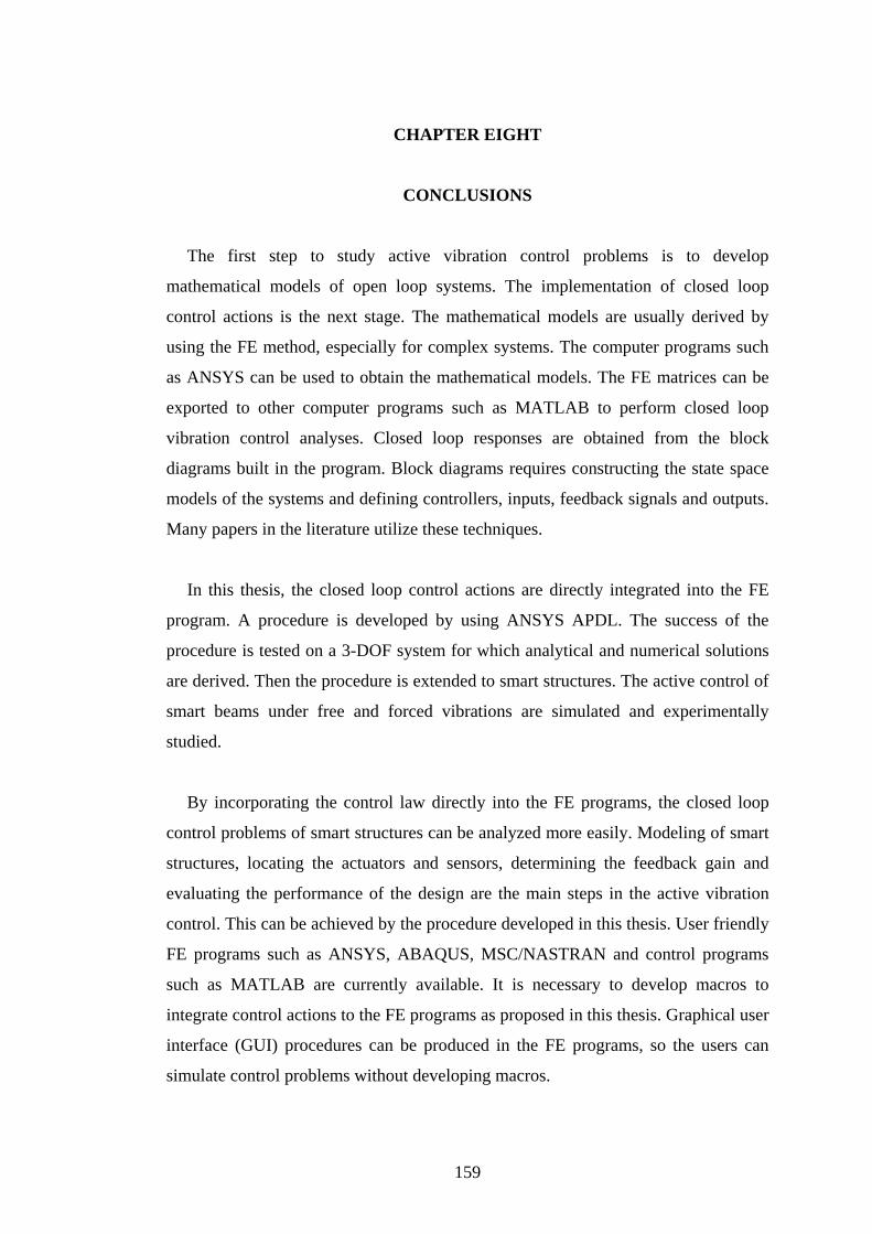
159
CHAPTER EIGHT
CONCLUSIONS
The first step to study active vibration control problems is to develop
mathematical models of open loop systems. The implementation of closed loop
control actions is the next stage. The mathematical models are usually derived by
using the FE method, especially for complex systems. The computer programs such
as ANSYS can be used to obtain the mathematical models. The FE matrices can be
exported to other computer programs such as MATLAB to perform closed loop
vibration control analyses. Closed loop responses are obtained from the block
diagrams built in the program. Block diagrams requires constructing the state space
models of the systems and defining controllers, inputs, feedback signals and outputs.
Many papers in the literature utilize these techniques.
In this thesis, the closed loop control actions are directly integrated into the FE
program. A procedure is developed by using ANSYS APDL. The success of the
procedure is tested on a 3-DOF system for which analytical and numerical solutions
are derived. Then the procedure is extended to smart structures. The active control of
smart beams under free and forced vibrations are simulated and experimentally
studied.
By incorporating the control law directly into the FE programs, the closed loop
control problems of smart structures can be analyzed more easily. Modeling of smart
structures, locating the actuators and sensors, determining the feedback gain and
evaluating the performance of the design are the main steps in the active vibration
control. This can be achieved by the procedure developed in this thesis. User friendly
FE programs such as ANSYS, ABAQUS, MSC/NASTRAN and control programs
such as MATLAB are currently available. It is necessary to develop macros to
integrate control actions to the FE programs as proposed in this thesis. Graphical user
interface (GUI) procedures can be produced in the FE programs, so the users can
simulate control problems without developing macros.

160
The following issues may be investigated in the future:
Active control of smart structures having complicated geometries can be
analyzed with the procedure proposed.
Optimal control laws can be incorporated into the FE models of smart
structures using the proposed technique.
Active control of smart structures can be studied using piezoelectric stack
(multi-layer) actuators. Studies may be extended to micro-positioning
applications by trajectory control.
The control of structures having different types of actuators such as fluid
power and servo motor can be simulated by the proposed techniques.
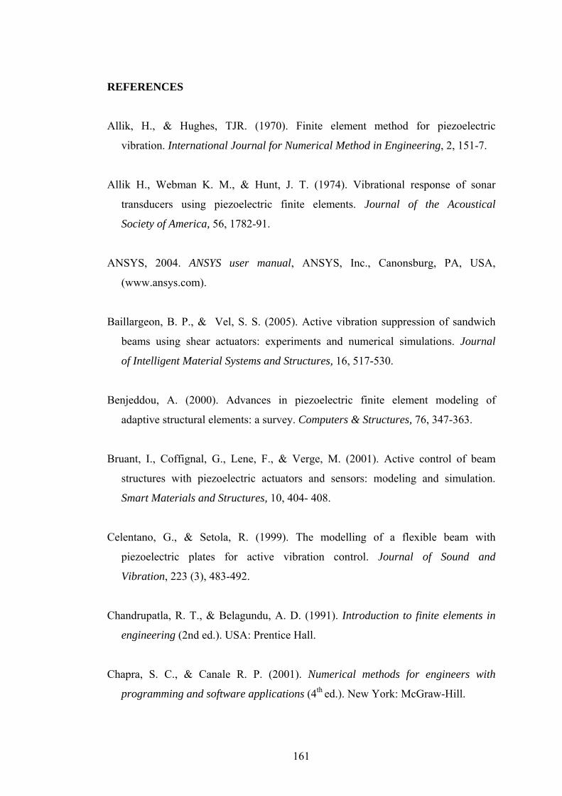
161
REFERENCES
Allik, H., & Hughes, TJR. (1970). Finite element method for piezoelectric
vibration. International Journal for Numerical Method in Engineering, 2, 151-7.
Allik H., Webman K. M., & Hunt, J. T. (1974). Vibrational response of sonar
transducers using piezoelectric finite elements. Journal of the Acoustical
Society of America, 56, 1782-91.
ANSYS, 2004. ANSYS user manual, ANSYS, Inc., Canonsburg, PA, USA,
(www.ansys.com).
Baillargeon, B. P., & Vel, S. S. (2005). Active vibration suppression of sandwich
beams using shear actuators: experiments and numerical simulations. Journal
of Intelligent Material Systems and Structures, 16, 517-530.
Benjeddou, A. (2000). Advances in piezoelectric finite element modeling of
adaptive structural elements: a survey. Computers & Structures, 76, 347-363.
Bruant, I., Coffignal, G., Lene, F., & Verge, M. (2001). Active control of beam
structures with piezoelectric actuators and sensors: modeling and simulation.
Smart Materials and Structures, 10, 404- 408.
Celentano, G., & Setola, R. (1999). The modelling of a flexible beam with
piezoelectric plates for active vibration control. Journal of Sound and
Vibration, 223 (3), 483-492.
Chandrupatla, R. T., & Belagundu, A. D. (1991). Introduction to finite elements in
engineering (2nd ed.). USA: Prentice Hall.
Chapra, S. C., & Canale R. P. (2001). Numerical methods for engineers with
programming and software applications (4th ed.). New York: McGraw-Hill.
162
Chin, L. C., Varadan V. V., & Varadan, V. K. (1994). Hybrid finite element
formulation for periodic piezoelectric arrays subjected to fluid loading.
International Journal for Numerical Method in Engineering, 37, 2987-3003.
Choi, S. B., Park, S. B., & Fukuda, T. (1998). A proof of concept investigation on
active vibration control of hybrid structures. Mechatronics, 8, 673-689.
Çalışkan, T. (2002). Smart materials and their applications in aerospace
structures. Ph.D Thesis. Middle East Technical University, TURKEY.
Dong, X. J., Meng, G., & Peng, J. C. (2006). Vibration control of piezoelectric
smart structures based on system identification technique: Numerical
simulation and experimental study. Journal of Sound and Vibration, 297, 680-
693.
Fariborzi, F., Golnaraghi, M. F., & Heppler, G. R. (1997). Experimental control of
free and forced structural vibration using a linear coupling strategy. Smart
Materials and Structures, 6, 540-548.
Fei, J. (2005). Active vibration control of flexible steel cantilever beam using
piezoelectric actuators. IEEE, 35-39.
Gabbert, U., Trajkov, T. M., & Köppe, H. (2002). Modelling, control and
simulation of piezoelectric smart structures using finite element method and
optimal control. Mechanics, Automatic Control and Robotics, 3, 417-430.
Gaudenzi, P., Carbonaro, R., & Benzi, E. (2000). Control of beam vibrations by
means of piezoelectric devices: theory and experiments. Composite Structures,
50, 373-379.
Ge, S. S., Lee, T H, & Gong, J. Q. (1999). A robust distributed controller of a
single link SCARA: Cartesian smart materials robot. Mechatronics, 9, 65-93
163
Ghandi K., & Hagood N. W. (1996). Nonlinear finite element modeing of phase
transitions in electro-mechanically coupled material. Smart Materials and
Structures, 2715, 121-140.
Ghandi, K., & Hagood, N. W. (1997). A hybrid finite element model for phase
transition in nonlinear electro-mechanically coupled material. Smart Materials
and Structures, 3039, 97-112.
Ha, S. K., Keilers C., & Chang F. K. (1992). Finite element analysis of composite
structures containing distributed piezoelectric sensors and actuators. AIAA
Journal, 30, 772-80.
Halim, D., & Moheimani, R. O. (2002). Experimental implementation of Spatial
Hinf control on a piezoelectric laminate beam. IEEE/Asme Transactions On
Mechatronics, 7, 346-356.
Hilal, M. A., Zibdeh, H. S. (2000). Vibration analysis of beams with general
boundary conditions traversed by a moving force. Journal of Sound and
Vibration, 229 (2), 377-388.
History of piezoelectricity (n.d.). Retrieved November 11, 2006, from
http://www.piezo.com/tech4history.html
Ikeda, T. (1996). Fundamentals of piezoelectricity. Oxford: Oxford University
Press
Jha, R., & Rower, J. (2002). Experimental investigation of active vibration control
using neural networks and piezoelectric actuators. Smart Materials and
Structures, 11, 115-121.
164
Karagülle, H., Malgaca, L., Öktem, H. F. (2004). Analysis of active vibration
control in smart structures by ANSYS. Smart Materials and Structures, 13,
661-667.
Kelly, S. G. (1993). Fundamentals of mechanical vibrations. Singapore:
McGraw-Hill.
Kıral, Z. (2002). Simulation and analysis of vibration signals generated by rolling
element bearings with defects. Ph.D Thesis. Dokuz EylülUniversity, TURKEY.
Kim, J., Varadan, V. V., Varadan, V. K. & Bao, X. Q. (1996). Finite element
modeling of a smart cantilever plate and comparison with experiments. Smart
Materials and Structures, 5, 165-170.
Koko I. S., Orisamolu I. R., Smith M. J., & Alepan U. O. (1997). Finite element
based design tool for smart composite structures. Smart Materials and
Structures, 3039, 125-134.
Kumar, R., & Singh, S. P. (2006). Adaptive hybrid control of smart structures
subjected to multiple disturbances. Smart Materials and Structures, 15, 1345-
1357.
Kuo, B. C. & Golnaraghi, F. (2003). Automatic control systems (8th ed.). USA: John
Wiley & Sons.
Kusculuoglu, Z. K., Fallahi, B., & Roston, T.J. (2004). Finite element model of a
beam with a piezoceramic actuator. Journal of Sound and Vibration, 276, 27-
44.
Lam, K. Y., Ng, T. Y. (1999). Active control of composite plates with integrated
piezoelectric sensors and actuators under various dynamic loading conditions.
Smart Materials and Structures, 8, 223-237.
165
LabVIEW (2003). LabVIEW user manual. National Instruments Corporation,
(www.ni.com).
Lim, Y-H., Varadan, V. V., & Varadan, V. K. (1997). Closed loop finite element
modeling of active structural damping in the frequency domain. Smart
Materials and Structures, 6, 161–8.
Lim, Y-H., Varadan, V. V., & Varadan, V. K. (1999). Closed loop finite element
modelling of active structural damping in the time domain. Smart
Materials and Structures, 8, 390–400.
Lim, Y. - H. (2003). Finite- element simulation of closed loop vibration control of
a smart plate under transient loading. Smart Materials and Structures, 12, 272-
286.
Lin, R. M., & Nyang, K. M. (2003). Analytical and experimental investigations on
vibrational control mechanisms for flexible active structures. Smart Materials
and Structures, 12, 500-506.
Ma, K., & Nejhad, M. N. G. (2005). Adaptive simultaneous precision positioning
and vibration control of intelligent composite structures. Journal of Intelligent
Material Systems and Structures, 16, 163-174.
Mackerle, J. (1998). Smart materials and structures-a finite element approach: a
bibliography (1986-1997). Modelling and Simulation in Materials Science and
Engineering, 6, 293-334.
Mackerle, J. (2003). Smart materials and structures-a finite element approach – an
addendum: a bibliography (1997-2002). Modelling and Simulation in
Materials Science and Engineering, 11, 707-744.
166
Manning, W. J., Plummer, A. R., & Levesley, M. C. (2000). Vibration control of a
flexible beam with integrated actuators and sensors. Smart Materials and
Structures, 9, 932-939.
MATLAB (2004). The MathWorks, Inc., United States, (www.mathworks.com).
Matsuzaki, Y. (1997). Smart structures research in Japan. Smart Materials and
Structures, 6, R1-R10.
Meng, G., Ye L., Dong, X-J., & Wei, K-X. (2006). Closed loop finite element
modeling of piezoelectric smart structures. Shock and Vibration, 13, 1-12.
Moita, J. M. S., Soares, C. M. M., & Soares, C. A. M. (2005). Active control of
forced vibrations in adaptive structures using a higher order model. Smart
Materials and Structures, 71, 349-355.
O’Connor, W., & Lang, D. (1998). Position control of flexible robot arms using
mechanical waves. Transactions of the ASME, 120, 334-339.
Prasad, E. (2002). Presentation of Eswar Prasad-Smart structures. Retrieved
January 11, 2005, from http://www.ae.metu.edu.tr/~yyaman/avt086/Prasad/.
Peng, F., Ng A. & Hu, Y.R., (2005). Actuator placement optimization and
adaptive vibration control of plate smart structures. Journal of Intelligent
Material Systems and Structures, 16, 263-271.
Preumont, A. (2002). Vibration control of active structures an introduction (2nd
ed.). Netherlands: Kluwer Academic Publishers.
Quek, S. T., Wang, S. Y., & Ang, K. K. (2003). Vibration control of composite
plates via optimal placement of piezoelectric patches. Journal of Intelligent
Material Systems and Structures, 14, 229- 245.
167
Raja, S., Prathap G., & Sihna, P. K. (2002). Active vibration control of composite
sandwich beams with piezoelectric extension-bending and shear actuators.
Smart Materials and Structures, 11, 63-71.
Reaves, C. M., & Horta, L. G. (2003). Piezoelectric actuator modeling using
MSC/NASTRAN and MATLAB. NASA/TM-2003-212651, Langley Research
Center, Hampton, Virginia.
Seba, B., Ni J. & Lohmann, B. (2006). Vibration attenuation using a piezoelectric
shunt circuit based on finite element method analysis. Smart Materials and
Structures, 15, 509-517.
Sekouri, E. M. (2004). Modellig and shape estimation of smart structures for
active control, Ph.D Thesis. Quebec Univesity, CANADA.
SensorTech (1983). Sensor Technology Limited, Ontario, Canada
(www.sensortech.ca).
Seto, K., & Matsumoto, Y. (1999, June). Active vibration control of multiple
buildings connected with active control bridges in response to large
earthquakes. Proceedings of the American Control Conference, 1007-1011.
Singh, S. P., Pruthi, H. S., & Agarwal, V. P. (2003). Efficient modal control
strategies for active control of vibrations. Journal of Sound and Vibration, 262,
563- 575.
Shin, H. C., & Choi, S. B., (2001). Position control of a two link flexible
manipulator featuring piezoelectric actuators and sensors. Mechatronics, 11,
707-729.
168
Sun, D., Mills, J. K, Shan, J., & Tsoa S. K. (2004). A PZT actuator control of a
single-link flexible manipulator based on linear velocity feedback and actuator
placement. Mechatronics, 14, 381-401.
Tzou, H. S., & Tseng, C. I. (1990). Distributed piezoelectric sensor/actuator
design for dynamic measurement/control of distributed parameter systems: A
piezoelectric finite element approach. Journal of Sound and Vibration, 138,
17-34.
Ülker, D. (2003). Active vibration control of smart structures. M.Sc Thesis.
Middle East Technical University, TURKEY.
Ülker, F. D., Yaman, Y., Nalbantoğlu V., & Kırcalı, Ö. F. (2005, June). Akıllı
bir plağın burulma titreşimlerinin aktif kontrolü. UMTS 2005, 12th National
Machine Theory Symposium, 1, 177-182.
Vasques, C. M. A., & Rodrigues, J. D. (2006). Active vibration control of smart
piezoelectric beams: comparison of classical and optimal feedback control
strategies. Computers & Structures, 84, 1402–1414
Williams, J. H. Jr. (1996) Fundamentals of applied dynamics. New York: John
Wiley & Sons.
Wu, J. J., Whittaker, A. R., & Cartmell M.P (2000). The use of finite element
techniques for calculating the dynamic response of structures to moving loads.
Composite & Structures, 78, 789-799.
Wu, J. J. (2003). Vibration of a rectangular plate undergoing forces moving along
a circular path. Finite Elements in Analysis and Design, 40, 41-60.
169
Xianmin, Z., Changjian, S., & Erdman, A. G. (2002). Active vibration controller
design and comparison study of flexible linkage mechanism systems.
Mechanisms and Machine Theory, 37, 985-997.
Xu, S. X., & Koko, T. S. (2004). Finite element analysis and design of actively
controlled piezoelectric smart structures. Finite Elements in Analysis and
Design, 40, 241-262.
Yaman, Y., Ülker, F. D., Nalbantoğlu, V., Çalışkan, T., Prasad, E., Waechter, D.,
& Yan, B. (2003). Application of μ synthesis active vibration control technique
to a smart fin. 6th CanSmart Workshop, 109-119, Canada.
Yang, S. M., Sheu, G. J., & Liu, K. C. (2005). Vibration control of composite
smart structures by feedforward adaptive filter in digital signal processor.
Journal of Intelligent Material Systems and Structures, 16, 773-779.
170
APPENDICES
APPENDIX A
SMART MATERIALS AND STRUCTURES
The most basic definition of a smart structure involves sensing of an
environmental change and the response to that change. Usually this process utilizes
electronic processing. In order to carry out these activities, a smart structure must
have the following components:
Sensor(s): Sensors are used to monitor environmental changes and generate
signal proportional to the changing property that can be measured.
Actuator(s): Actuators are used to change the properties of the smart structure
in order to achieve the desired response.
Control System(s): Control systems continually monitor the sensor’s signal,
processing the information in order to determine if action is required. If an
action is required, then a signal is applied to the appropriate actuator(s).
The schematic view of a smart structure is shown in Figure A.1. If the set of
actuators and sensors are located at discrete points of the structure, they can be
treated separately. The distinctive feature of smart structures is that the actuators
and sensors are distributed and have a high degree of integration inside the
structure, which makes a separate modeling impossible.
Figure A.1 Smart structure.
171
From a mechanical point of view, classical structural materials are entirely
described by their elastic constants relating stress and strain, and their thermal
expansion coefficient relating the strain to the temperature. Smart materials are
materials where strain can also be generated by different mechanisms involving
electric field, magnetic field, temperature, etc. as a result of some coupling in their
constitutive equations. More detailed information on the types of the smart materials
and their application areas can be found in the references (Çalışkan, 2002, Prasad,
2002, Sekouri, 2004, Ülker, 2003).
Although this thesis is entirely devoted piezoelectric smart structures, brief
information on the types of smart materials used as actuator and sensor, examples of
their applications are given in the following sections.
A.1 Components of Smart Structures
A.1.1 Actuators
A number of different actuator can be incorporated into a smart structure in order
to generate an appropriate response to a detected environmental variation. The
different types of smart materials used as actuators may be classified in terms of
driving energy as given in Table A.1.
Table A.1 Types of smart materials.
Property Actuators Driving Energy Devices
Shape Memory Nitinol T,S Strip, Spring Tube
Magnetostriction Terfenol- D H Rod, Stack, Wire
Piezoelectric
Electrostrictive
BT,PZT
PMN E,S
Disc, Plate, Stack,
Tube, Cylinder
Electrorheological E Plate, Cylinder
T: Thermal energy S: Mechanical strain H: Magnetic field E: Electric field
172
A.1.1.1 Shape Memory Alloys (SMA)
The term “shape-memory” is used to describe the ability of a material to regain its
original shape when heated to a higher temperature, after being deformed at a lower
temperature. The shape memory effect occurs in a number of alloys, which undergo a
special type of phase transformation called “thermoelastic martensite
transformation”.
Shape memory alloys allow one to recover up to 5 % strain from the phase change
induced by temperature. Although two way applications are possible after education,
SMAs are best suited to one-way tasks such as deployment. The best known SMA is
the NITINOL. SMAs are little used in vibration control. They can be used only at
low frequency and low precision applications, mainly because of the difficulty of
cooling. Fatigue under thermal cycling is also problem. Applications of SMAs are
listed below:
• Automobile Transmissions: Control of a automatic transmissions in cold
weather due to the change in oil viscosity.
• Shock Absorbers: Improve low temperature properties of shock absorbers by
controlling their pressure valves.
• Small Pumps: Laser controlled shape-memory alloy actuators drive a
cantilever beam that operates a pump.
A.1.1.2 Magnetostrictive Materials
Magnetostriction is a transduction process in which electrical energy is converted
to mechanical energy. Magnetostrictive materials exhibit a change in dimension
when placed in a magnetic field. The maximum response is obtained when the
material is subjected to compressive loads. Magnetostrictive actuators can be used as
load carrying elements (in compressing alone) and they have a long life time. The
best known is the TERFENOL-D. They can also be used in high precision
applications. Applications of magnetostrictive materials are listed below:
173
• Hydraulic Valves: High speed valves, operating at frequencies of 1 kHz,
displace 3 mm at 300 Hz. They can generate pressure changes of 100 Psi at
2000 Psi operating pressures.
• Inchworm Motors: Motors can generate a torque of 12 Nm directly off its
shaft at 0.5 rpm. Applications are in low frequency acoustic transducers,
pumps and mechanical systems.
• Helicopter Rotors: Potential application in active control of vibration in
trailing edge flaps by modifying their shape.
A.1.1.3 Magneto-rheological Materials (MR)
MR fluids consist of viscous fluids containing micron-sized particles of magnetic
material. When the fluids subjected to a magnetic field, the particles create columnar
structures requiring a minimum shear stress to initiate the flow. The effect is
reversible and very fast (response time of the order of millisecond). Some fluids
exhibit the same behaviour under electric field; they are called Electro-rheological
(ER) fluids; however, their performances (limited by the electric field break-down)
are significantly inferior to MR fluids. ER materials exist in a wide variety of
colloidal suspensions of dielectric solids in non-conducting liquids. In the absence of
electric field, the colloidal suspension is composed of fine particles (0.1 – 1.0 μm)
which are uniformly distributed throughout the field. When an electric field is
applied, the dielectric properties of the particles cause them to align with the electric
field and cause them to adhere to adjacent particles which join to form fibrils. The
presence of these fibrils considerably modifies the viscosity of the fluid (by as much
as a factor of 50). The alignment disappears when the electric field is removed, thus
creating the desired property of complete cyclic reproducibility. Applications of ER
materials are listed below:
• Static Mode: Release mechanisms.
• Shear Mode: Clutch devices, ER fluids mechanically couples two surfaces by
increasing or decreasing their viscosity with the application or removal of an
electric field.
174
• Damping Devices: Shock absorbers. ER fluid usually operates in either the
shear or extensional configuration is used when the fluid undergoes strain,
and extensional configuration used for compression stress.
• Variable Flow Controls: Adjusting the viscosity of a fluid as it flows through
a porous electrode separating two chambers can control the volume of flow.
A.1.1.4 Piezoelectric Materials
Piezoelectric materials have recoverable strain of 0.1 % under electric field. They
can be used as actuators as well as sensors. Piezoelectric behaviour can be revealed
in two distinct ways. There are two broad classes of piezoelectric materials used in
vibration control: ceramic and polymers. The types of piezoelectric materials can be
listed in Table A.2.
• Direct piezoelectric effect: This effect occurs when a piezoelectric material
becomes electrically charged when subjected to a mechanical stress.
• Converse piezoelectric effect: This effect occurs when the piezoelectric
material becomes strained when placed in an electric field.
Table A.2 Piezoelectric materials.
Type Materials
Single
Crystals
Quartz
Lead Magnesium Niobate
(PMN-PT and PZN-PT)
Ceramics
Lead Zirconate Titanate (PZT)
Lead Metariobate (LMN)
Lead Titanate (LT)
Lead Magnesium Niobate (PMN)
Polymers Polyvinylenedifluoride (PVDF)
CompositesCeramic-polymer
Ceramic-Glass
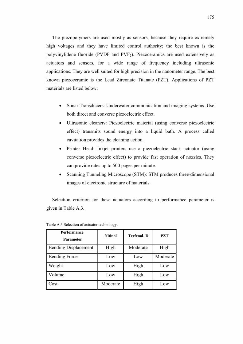
175
The piezopolymers are used mostly as sensors, because they require extremely
high voltages and they have limited control authority; the best known is the
polyvinylidene fluoride (PVDF and PVF2). Piezoceramics are used extensively as
actuators and sensors, for a wide range of frequency including ultrasonic
applications. They are well suited for high precision in the nanometer range. The best
known piezoceramic is the Lead Zirconate Titanate (PZT). Applications of PZT
materials are listed below:
• Sonar Transducers: Underwater communication and imaging systems. Use
both direct and converse piezoelectric effect.
• Ultrasonic cleaners: Piezoelectric material (using converse piezoelectric
effect) transmits sound energy into a liquid bath. A process called
cavitation provides the cleaning action.
• Printer Head: Inkjet printers use a piezoelectric stack actuator (using
converse piezoelectric effect) to provide fast operation of nozzles. They
can provide rates up to 500 pages per minute.
• Scanning Tunneling Microscope (STM): STM produces three-dimensional
images of electronic structure of materials.
Selection criterion for these actuators according to performance parameter is
given in Table A.3.
Table A.3 Selection of actuator technology.
Performance
Parameter Nitinol Terfenol- D PZT
Bending Displacement High Moderate High
Bending Force Low Low Moderate
Weight Low High Low
Volume Low High Low
Cost Moderate High Low
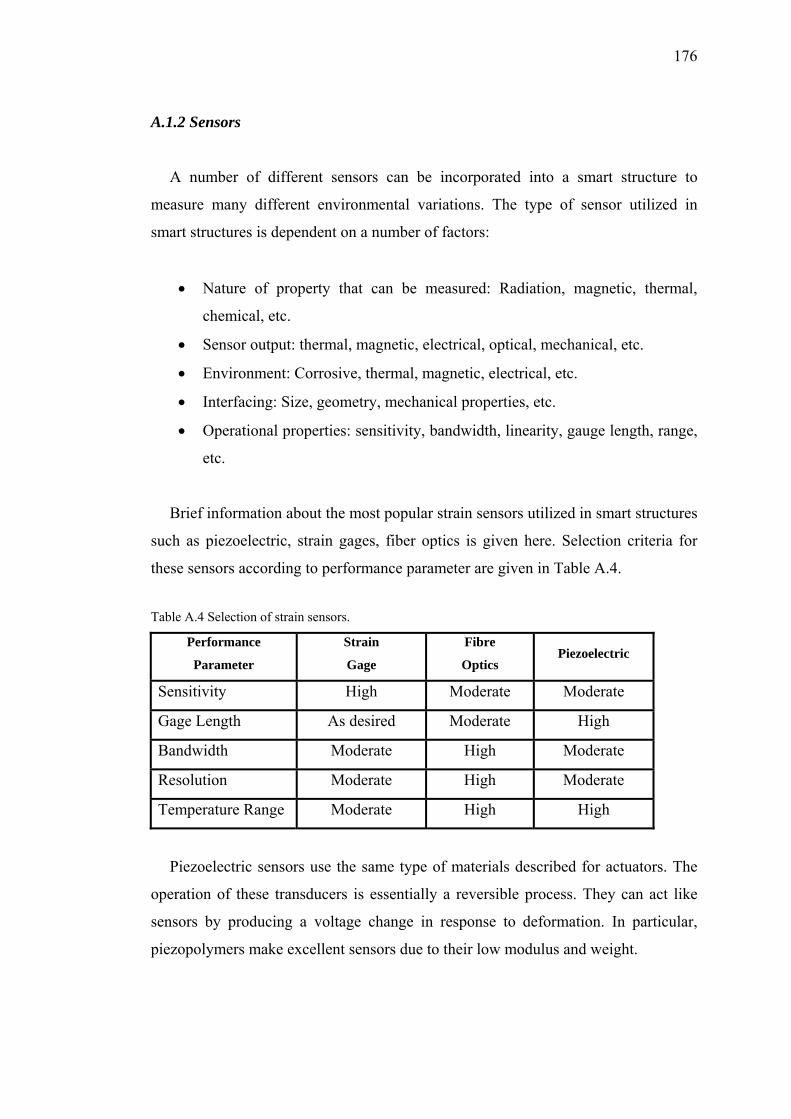
176
A.1.2 Sensors
A number of different sensors can be incorporated into a smart structure to
measure many different environmental variations. The type of sensor utilized in
smart structures is dependent on a number of factors:
• Nature of property that can be measured: Radiation, magnetic, thermal,
chemical, etc.
• Sensor output: thermal, magnetic, electrical, optical, mechanical, etc.
• Environment: Corrosive, thermal, magnetic, electrical, etc.
• Interfacing: Size, geometry, mechanical properties, etc.
• Operational properties: sensitivity, bandwidth, linearity, gauge length, range,
etc.
Brief information about the most popular strain sensors utilized in smart structures
such as piezoelectric, strain gages, fiber optics is given here. Selection criteria for
these sensors according to performance parameter are given in Table A.4.
Table A.4 Selection of strain sensors.
Performance
Parameter
Strain
Gage
Fibre
Optics Piezoelectric
Sensitivity High Moderate Moderate
Gage Length As desired Moderate High
Bandwidth Moderate High Moderate
Resolution Moderate High Moderate
Temperature Range Moderate High High
Piezoelectric sensors use the same type of materials described for actuators. The
operation of these transducers is essentially a reversible process. They can act like
sensors by producing a voltage change in response to deformation. In particular,
piezopolymers make excellent sensors due to their low modulus and weight.
177
Strain gages are simple and inexpensive sensors, and represent a mature
technology. Since they are discrete devices, they may be difficult to embed in a
composite type structure. This problem can be overcome by producing a thin film
with gages printed on it at regular intervals. Subsequently, it is bonded to the wall of
structure during the manufacturing process.
Fiber Optic sensors can be made extremely small and can be embedded into
composite materials without structural degradation. Because of the high melting
point of these fibers and high inherent strength of glass, they are able to operate in
extremely hostile environments at high temperatures, vibrations and shock loadings.
Fiber Optic sensors can be used to detect heat or stress. Two types of fiber-optic
sensors are used, intrinsic and extrinsic types. In the extrinsic type, fiber acts as
medium of transmission. In the intrinsic type, one or more field parameters become
modulated with the field which propagates in the fiber to allow the measurement of
environmental effects.
A.1.3 Control Systems
A smart control system provides feedback control for the sensors and actuators.
The control system should have the following properties:
• Analogue-to-digital (ADC) and digital-to-analogue (DAC) converters.
• Input signal amplification, filtering and output power supply.
• Control algorithm.
• Digital signal processor (DSP).
178
A.2 Piezoelectric Constitutive Equations
In an unstressed one-dimensional dielectric medium, the electric displacement D
(charge per unit area, expressed in C/m2) is related to the electric field E (V/m) by
D = eE (A.1)
where e is the dielectric constant of the material (Preumont, 2002).
Similarly in a one-dimensional elastic body placed in a zero electric field, the strain S
and the stress T (N/m2) are related by
S = sT (A.2)
where s is the compliance of the material (inverse of the Young modulus). For a
piezoelectric material, the electrical and mechanical constitutive equations are
coupled.
S = sE T + d E (A.3)
D = d T + εT E (A.4)
In Equation (A.3), the piezoelectric constant d relates the strain to the electric
field E in the absence of mechanical stress and sE refers is the compliance when the
electric field is constant. In Equation (A.4), d relates the electric displacement to the
stress under a zero electric field (short-circuit electrodes); d is expressed in (m/V or
Coulomb/Newton). eT is the dielectric constant under constant stress. The above
equations can be transformed into
E)sd1(S
sdD
EsdS
s1T
TE
2T
E
EE
ε−ε+=
−=
(A.5)
(A.6)
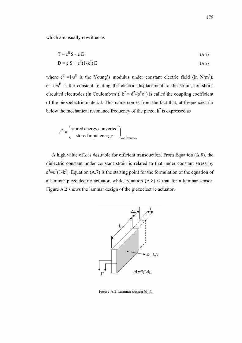
179
which are usually rewritten as
T = cE S - e E (A.7)
D = e S + εT(1-k2) E (A.8)
where cE =1/sE is the Young’s modulus under constant electric field (in N/m2);
e= d/sE is the constant relating the electric displacement to the strain, for short-
circuited electrodes (in Coulomb/m2). k2 = d2/(sEeT) is called the coupling coefficient
of the piezoelectric material. This name comes from the fact that, at frequencies far
below the mechanical resonance frequency of the piezo, k2 is expressed as
frequencylow
2
energyinput storedconvertedenergy storedk ⎟⎟
⎠
⎞⎜⎜⎝
⎛=
A high value of k is desirable for efficient transduction. From Equation (A.8), the
dielectric constant under constant strain is related to that under constant stress by
εS=εT(1-k2). Equation (A.7) is the starting point for the formulation of the equation of
a laminar piezoelectric actuator, while Equation (A.8) is that for a laminar sensor.
Figure A.2 shows the laminar design of the piezoelectric actuator.
Figure A.2 Laminar design (d31).
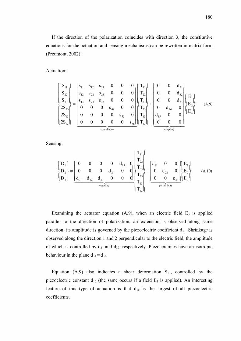
180
If the direction of the polarization coincides with direction 3, the constitutive
equations for the actuation and sensing mechanisms can be rewritten in matrix form
(Preumont, 2002):
Actuation:
⎪⎭
⎪⎬
⎫
⎪⎩
⎪⎨
⎧
⎥⎥⎥⎥⎥⎥⎥⎥
⎦
⎤
⎢⎢⎢⎢⎢⎢⎢⎢
⎣
⎡
+
⎪⎪⎪⎪
⎭
⎪⎪⎪⎪
⎬
⎫
⎪⎪⎪⎪
⎩
⎪⎪⎪⎪
⎨
⎧
⎥⎥⎥⎥⎥⎥⎥⎥
⎦
⎤
⎢⎢⎢⎢⎢⎢⎢⎢
⎣
⎡
=
⎪⎪⎪⎪
⎭
⎪⎪⎪⎪
⎬
⎫
⎪⎪⎪⎪
⎩
⎪⎪⎪⎪
⎨
⎧
3
2
1
coupling
15
24
33
32
31
12
13
23
33
22
11
compliance
66
55
44
332313
232212
131211
12
13
23
33
22
11
EEE
00000d0d0
d00d00d00
TTTTTT
s000000s000000s000000sss000sss000sss
S2S2S2SSS
44 344 2144444 344444 21
(A.9)
Sensing:
⎪⎭
⎪⎬
⎫
⎪⎩
⎪⎨
⎧
⎥⎥⎥
⎦
⎤
⎢⎢⎢
⎣
⎡
εε
ε+
⎪⎪⎪⎪
⎭
⎪⎪⎪⎪
⎬
⎫
⎪⎪⎪⎪
⎩
⎪⎪⎪⎪
⎨
⎧
⎥⎥⎥
⎦
⎤
⎢⎢⎢
⎣
⎡=
⎪⎭
⎪⎬
⎫
⎪⎩
⎪⎨
⎧
3
2
1
typermittivi
33
22
11
12
13
23
33
22
11
coupling
333231
24
15
3
2
1
EEE
000000
TTTTTT
000ddd00d0000d0000
DDD
44 344 2144444 344444 21
(A.10)
Examining the actuator equation (A.9), when an electric field E3 is applied
parallel to the direction of polarization, an extension is observed along same
direction; its amplitude is governed by the piezoelectric coefficient d33. Shrinkage is
observed along the direction 1 and 2 perpendicular to the electric field, the amplitude
of which is controlled by d31 and d32, respectively. Piezoceramics have an isotropic
behaviour in the plane d31 = d32.
Equation (A.9) also indicates a shear deformation S13, controlled by the
piezoelectric constant d15 (the same occurs if a field E1 is applied). An interesting
feature of this type of actuation is that d15 is the largest of all piezoelectric
coefficients.
181
A.3 The Finite Element Method
Analytical solutions of piezoelectric smart structures performance generally
examine simple shapes under static or dynamic conditions. Analytical solutions of
complex geometries often involve assumptions which simplify the stress state and
electric field distribution within the structure. Invariably, this leads to inaccurate
predictions of the observed response. The advantage of the FE analysis over
analytical solutions is that stress and electrical field measurements of complex
geometries, and their variations throughout the structure are more readily calculated.
The FE analysis allows calculation of the stress and electric field distributions under
static, dynamic, and electrical loads. Therefore, the performance of the structure can
be evaluated and optimized before manufacturing process.
A.3.1 Piezoelectric Elements in ANSYS
ANSYS FE-program offers two and three dimensional piezoelectric coupled-field
elements for modeling structures with piezoelectric actuators/sensors. Static, modal,
full harmonic and transient analysis can be performed with this commercial software.
Plane and solid piezoelectric elements are available in ANSYS (ANSYS, 2004).
They have the capability of modeling piezoelectric response. ANSYS (version 10)
has six specific coupled field elements for piezoelectric analysis:
PLANE 13 – 2D Coupled-field solid element
PLANE 223 – 2D 8-Node coupled-field solid element
SOLID5 - 3D Coupled-field solid element
SOLID98 - Tetrahedral coupled-field solid element
SOLID226- 3D 20-Node coupled-field solid element
SOLID227- 3D 20-Node coupled-field solid element
For a piezoelectric element there are four DOF at each node; ux, uy, uz and volt. In
this case, it is necessary to use ‘coupled-field analysis’ to couple the interaction
between applied stress and electric field.
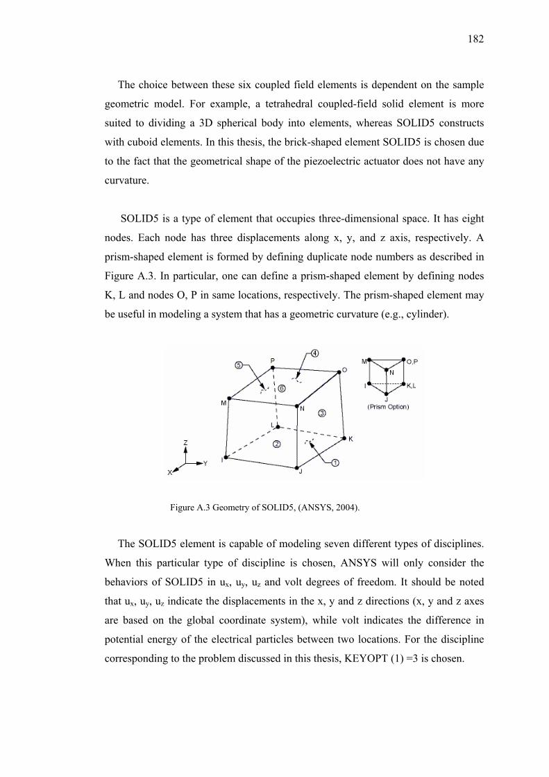
182
The choice between these six coupled field elements is dependent on the sample
geometric model. For example, a tetrahedral coupled-field solid element is more
suited to dividing a 3D spherical body into elements, whereas SOLID5 constructs
with cuboid elements. In this thesis, the brick-shaped element SOLID5 is chosen due
to the fact that the geometrical shape of the piezoelectric actuator does not have any
curvature.
SOLID5 is a type of element that occupies three-dimensional space. It has eight
nodes. Each node has three displacements along x, y, and z axis, respectively. A
prism-shaped element is formed by defining duplicate node numbers as described in
Figure A.3. In particular, one can define a prism-shaped element by defining nodes
K, L and nodes O, P in same locations, respectively. The prism-shaped element may
be useful in modeling a system that has a geometric curvature (e.g., cylinder).
Figure A.3 Geometry of SOLID5, (ANSYS, 2004).
The SOLID5 element is capable of modeling seven different types of disciplines.
When this particular type of discipline is chosen, ANSYS will only consider the
behaviors of SOLID5 in ux, uy, uz and volt degrees of freedom. It should be noted
that ux, uy, uz indicate the displacements in the x, y and z directions (x, y and z axes
are based on the global coordinate system), while volt indicates the difference in
potential energy of the electrical particles between two locations. For the discipline
corresponding to the problem discussed in this thesis, KEYOPT (1) =3 is chosen.
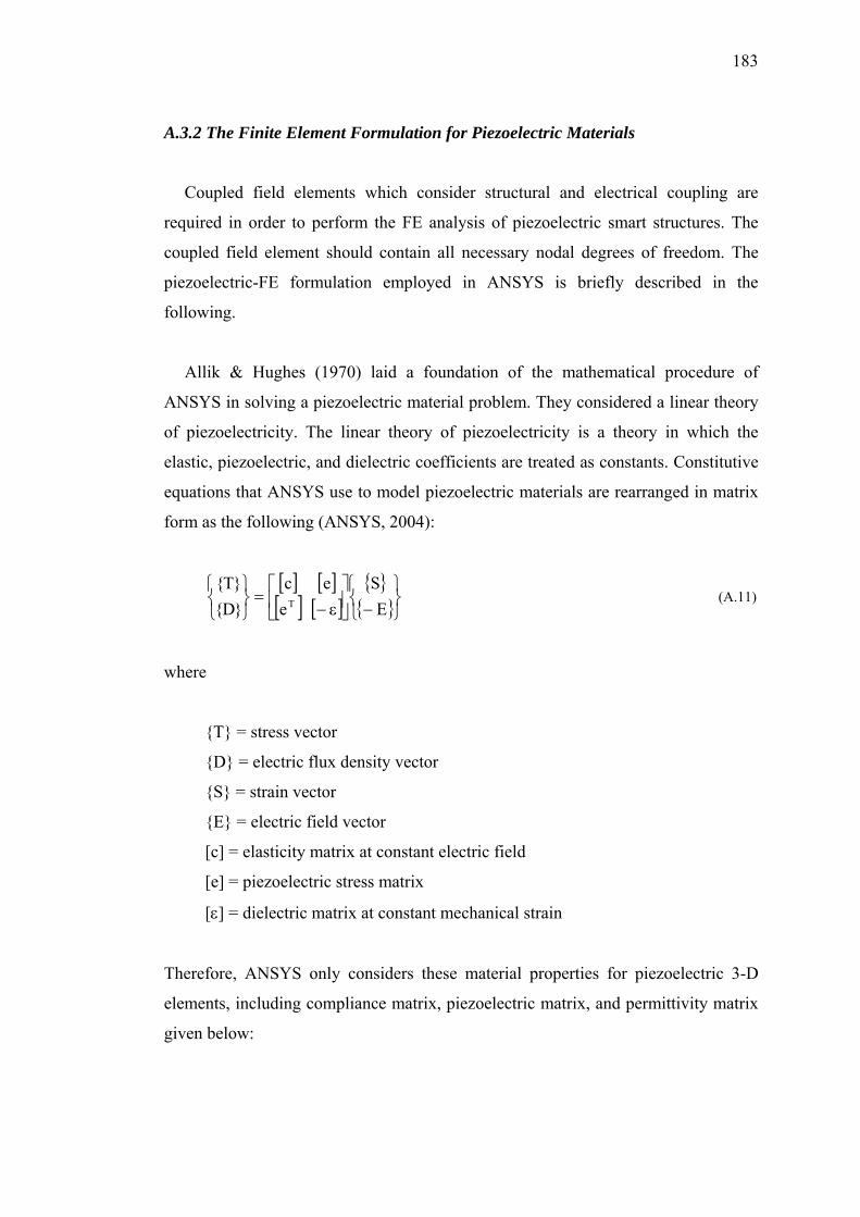
183
A.3.2 The Finite Element Formulation for Piezoelectric Materials
Coupled field elements which consider structural and electrical coupling are
required in order to perform the FE analysis of piezoelectric smart structures. The
coupled field element should contain all necessary nodal degrees of freedom. The
piezoelectric-FE formulation employed in ANSYS is briefly described in the
following.
Allik & Hughes (1970) laid a foundation of the mathematical procedure of
ANSYS in solving a piezoelectric material problem. They considered a linear theory
of piezoelectricity. The linear theory of piezoelectricity is a theory in which the
elastic, piezoelectric, and dielectric coefficients are treated as constants. Constitutive
equations that ANSYS use to model piezoelectric materials are rearranged in matrix
form as the following (ANSYS, 2004):
[ ] [ ][ ] [ ]
{ }{ }⎭
⎬⎫
⎩⎨⎧−⎥
⎦
⎤⎢⎣
⎡ε−
=⎭⎬⎫
⎩⎨⎧
ES
eec
}D{}T{
T (A.11)
where
{T} = stress vector
{D} = electric flux density vector
{S} = strain vector
{E} = electric field vector
[c] = elasticity matrix at constant electric field
[e] = piezoelectric stress matrix
[ε] = dielectric matrix at constant mechanical strain
Therefore, ANSYS only considers these material properties for piezoelectric 3-D
elements, including compliance matrix, piezoelectric matrix, and permittivity matrix
given below:
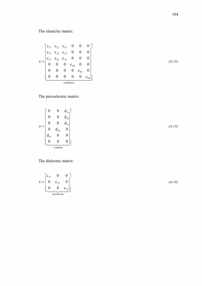
184
The elasticity matrix:
44444 344444 21compliance
66
55
44
332313
232212
131211
c000000c000000c000000ccc000ccc000ccc
c
⎥⎥⎥⎥⎥⎥⎥⎥
⎦
⎤
⎢⎢⎢⎢⎢⎢⎢⎢
⎣
⎡
= (A.12)
The piezoelectric matrix:
44 344 21coupling
15
24
33
32
31
00000d0d0
d00d00d00
e
⎥⎥⎥⎥⎥⎥⎥⎥
⎦
⎤
⎢⎢⎢⎢⎢⎢⎢⎢
⎣
⎡
= (A.13)
The dielectric matrix:
44 344 21typermittivi
33
22
11
000000
⎥⎥⎥
⎦
⎤
⎢⎢⎢
⎣
⎡
εε
ε=ε (A.14)
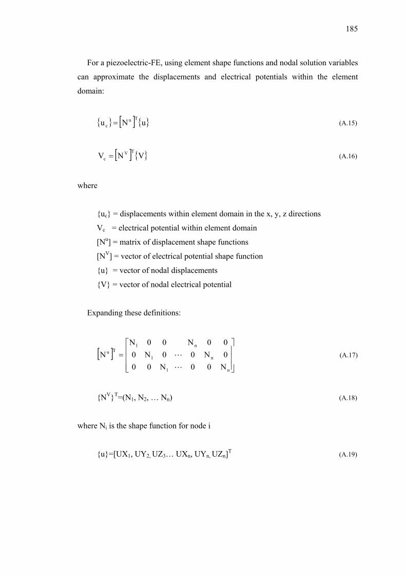
185
For a piezoelectric-FE, using element shape functions and nodal solution variables
can approximate the displacements and electrical potentials within the element
domain:
{ } [ ] { }uNu Tuc = (A.15)
[ ] { }VNV TVc = (A.16)
where
{uc} = displacements within element domain in the x, y, z directions
Vc = electrical potential within element domain
[Nu] = matrix of displacement shape functions
[NV] = vector of electrical potential shape function
{u} = vector of nodal displacements
{V} = vector of nodal electrical potential
Expanding these definitions:
[ ]⎥⎥⎥
⎦
⎤
⎢⎢⎢
⎣
⎡=
n1
n1
n1Tu
N00N000N00N000N00N
NL
L (A.17)
{NV}T=(N1, N2, … Nn) (A.18)
where Ni is the shape function for node i
{u}=[UX1, UY2, UZ3… UXn, UYn, UZn]T (A.19)
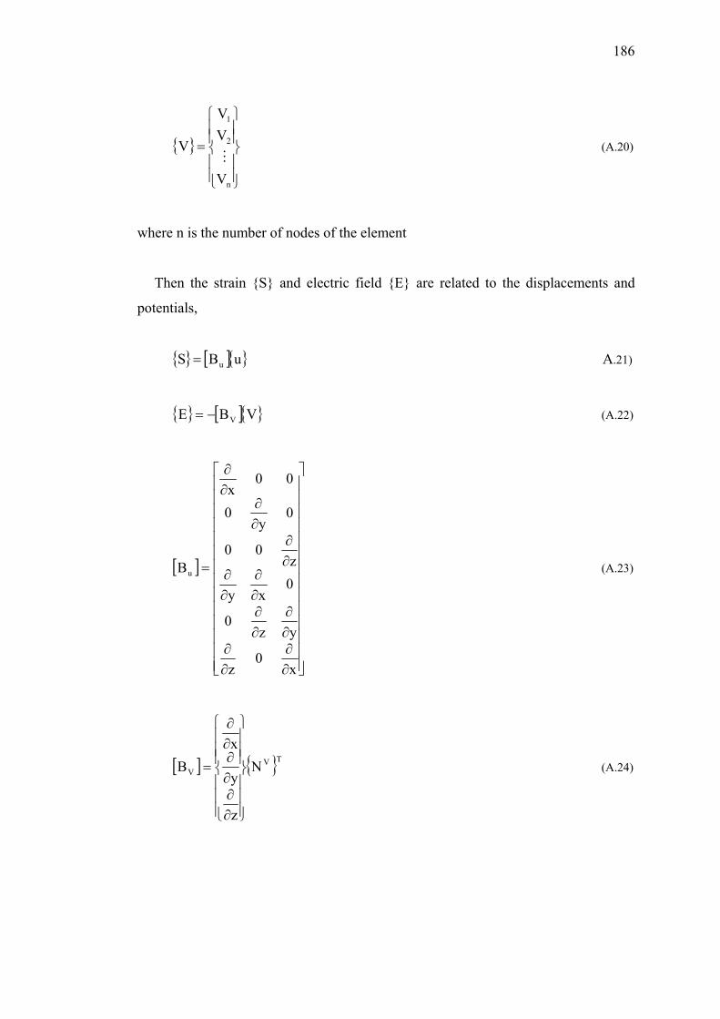
186
{ }
⎪⎪⎭
⎪⎪⎬
⎫
⎪⎪⎩
⎪⎪⎨
⎧
=
n
2
1
V
VV
VM
(A.20)
where n is the number of nodes of the element
Then the strain {S} and electric field {E} are related to the displacements and
potentials,
{ } [ ]{ }uBS u= A.21)
{ } [ ]{ }VBE V−= (A.22)
[ ]
⎥⎥⎥⎥⎥⎥⎥⎥⎥⎥⎥⎥⎥⎥
⎦
⎤
⎢⎢⎢⎢⎢⎢⎢⎢⎢⎢⎢⎢⎢⎢
⎣
⎡
∂∂
∂∂
∂∂
∂∂∂∂
∂∂
∂∂
∂∂
∂∂
=
x0
z
yz0
0xy
z00
0y
0
00x
Bu (A.23)
[ ] { }TVV N
z
y
xB
⎪⎪⎪
⎭
⎪⎪⎪
⎬
⎫
⎪⎪⎪
⎩
⎪⎪⎪
⎨
⎧
∂∂∂∂∂∂
= (A.24)
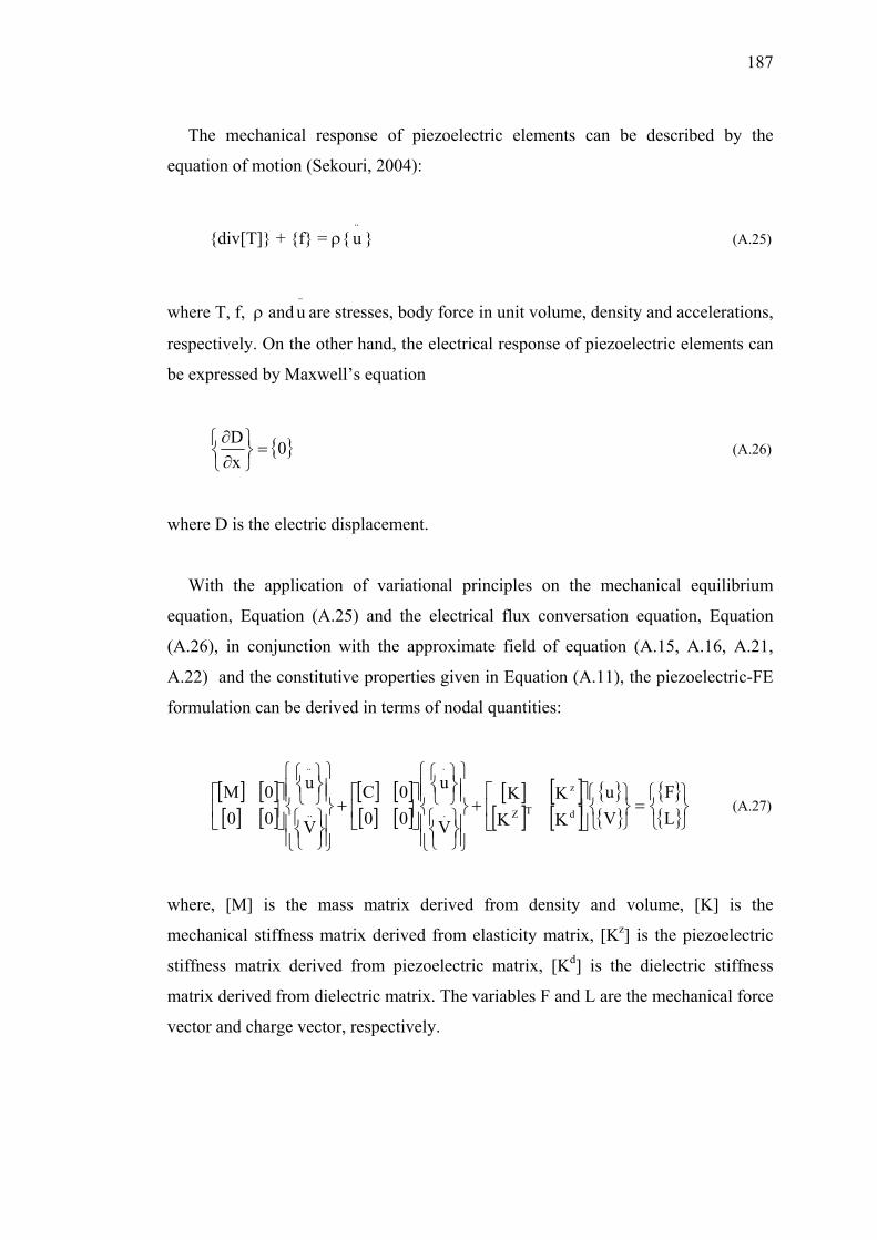
187
The mechanical response of piezoelectric elements can be described by the
equation of motion (Sekouri, 2004):
{div[T]} + {f} = ρ{⋅⋅
u } (A.25)
where T, f, ρ and⋅⋅
u are stresses, body force in unit volume, density and accelerations,
respectively. On the other hand, the electrical response of piezoelectric elements can
be expressed by Maxwell’s equation
{ }0xD
=⎭⎬⎫
⎩⎨⎧∂∂ (A.26)
where D is the electric displacement.
With the application of variational principles on the mechanical equilibrium
equation, Equation (A.25) and the electrical flux conversation equation, Equation
(A.26), in conjunction with the approximate field of equation (A.15, A.16, A.21,
A.22) and the constitutive properties given in Equation (A.11), the piezoelectric-FE
formulation can be derived in terms of nodal quantities:
[ ] [ ][ ] [ ]
[ ] [ ][ ] [ ]
[ ] [ ][ ] [ ]
{ }{ }
{ }{ }⎭
⎬⎫
⎩⎨⎧
=⎭⎬⎫
⎩⎨⎧⎥⎦
⎤⎢⎣
⎡+
⎪⎪⎭
⎪⎪⎬
⎫
⎪⎪⎩
⎪⎪⎨
⎧
⎭⎬⎫
⎩⎨⎧
⎭⎬⎫
⎩⎨⎧
⎥⎦
⎤⎢⎣
⎡+
⎪⎪⎭
⎪⎪⎬
⎫
⎪⎪⎩
⎪⎪⎨
⎧
⎭⎬⎫
⎩⎨⎧
⎭⎬⎫
⎩⎨⎧
⎥⎦
⎤⎢⎣
⎡⋅⋅⋅
LF
Vu
KKKK
V
u
000C
V
u
000M
dTZ
z
... (A.27)
where, [M] is the mass matrix derived from density and volume, [K] is the
mechanical stiffness matrix derived from elasticity matrix, [Kz] is the piezoelectric
stiffness matrix derived from piezoelectric matrix, [Kd] is the dielectric stiffness
matrix derived from dielectric matrix. The variables F and L are the mechanical force
vector and charge vector, respectively.
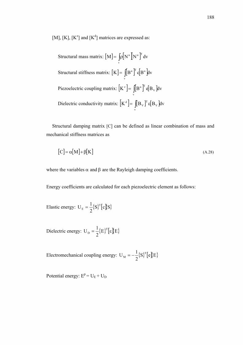
188
[M], [K], [Kz] and [Kd] matrices are expressed as:
Structural mass matrix: [ ] [ ][ ]∫ρ=v
Tuu dvNNM
Structural stiffness matrix: [ ] [ ] [ ]∫=v
uTu dvBcBK
Piezoelectric coupling matrix: [ ] [ ] [ ]∫=v
VTuz dvBeBK
Dielectric conductivity matrix: [ ] [ ] [ ]∫ ε=v
VT
Vd dvBBK
Structural damping matrix [C] can be defined as linear combination of mass and
mechanical stiffness matrices as
[ ] [ ] [ ]KMC β+α= (A.28)
where the variables α and β are the Rayleigh damping coefficients.
Energy coefficients are calculated for each piezoelectric element as follows:
Elastic energy: { } [ ]{ }ScS21U T
E =
Dielectric energy: { } [ ]{ }EE21U T
D ε=
Electromechanical coupling energy: { } [ ]{ }EeS21U T
M −=
Potential energy: Ep = UE + UD
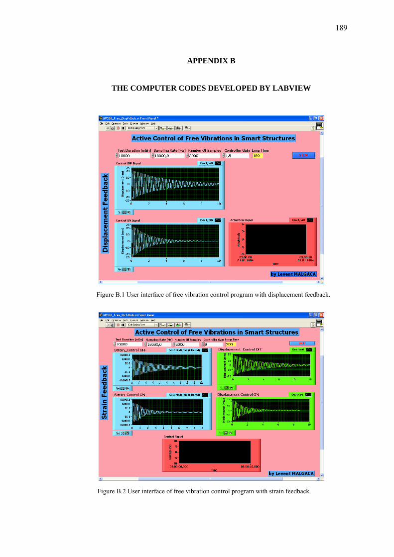
189
APPENDIX B
THE COMPUTER CODES DEVELOPED BY LABVIEW
Figure B.1 User interface of free vibration control program with displacement feedback.
Figure B.2 User interface of free vibration control program with strain feedback.
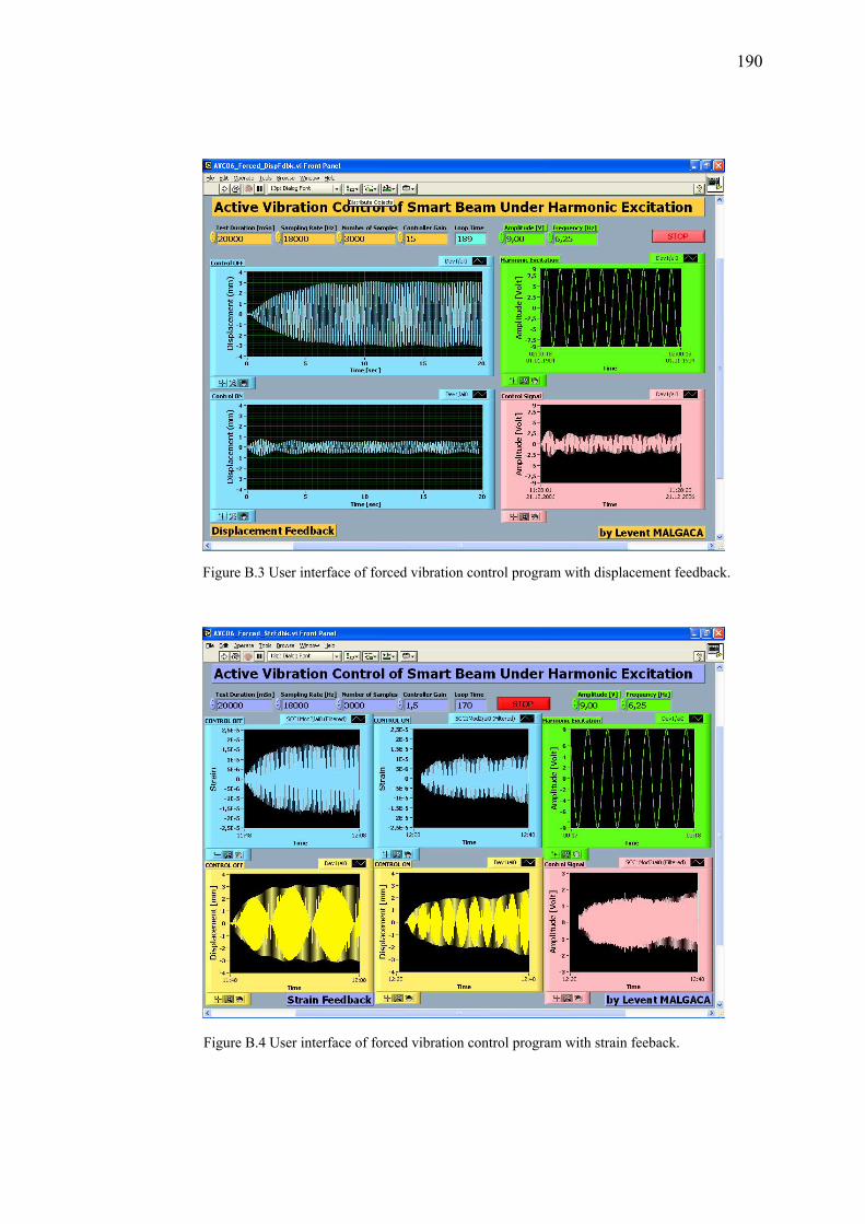
190
Figure B.3 User interface of forced vibration control program with displacement feedback.
Figure B.4 User interface of forced vibration control program with strain feeback.
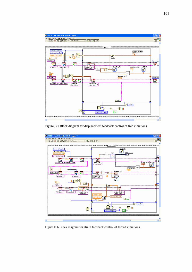
191
Figure B.5 Block diagram for displacement feedback control of free vibrations.
Figure B.6 Block diagram for strain feedback control of forced vibrations.
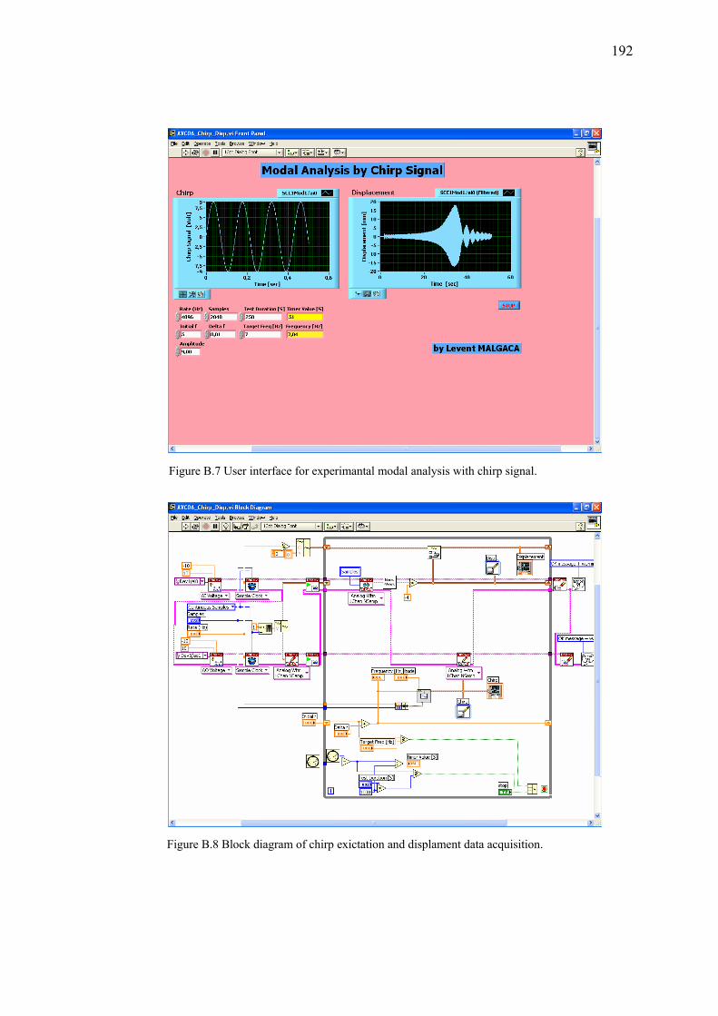
192
Figure B.7 User interface for experimantal modal analysis with chirp signal.
Figure B.8 Block diagram of chirp exictation and displament data acquisition.
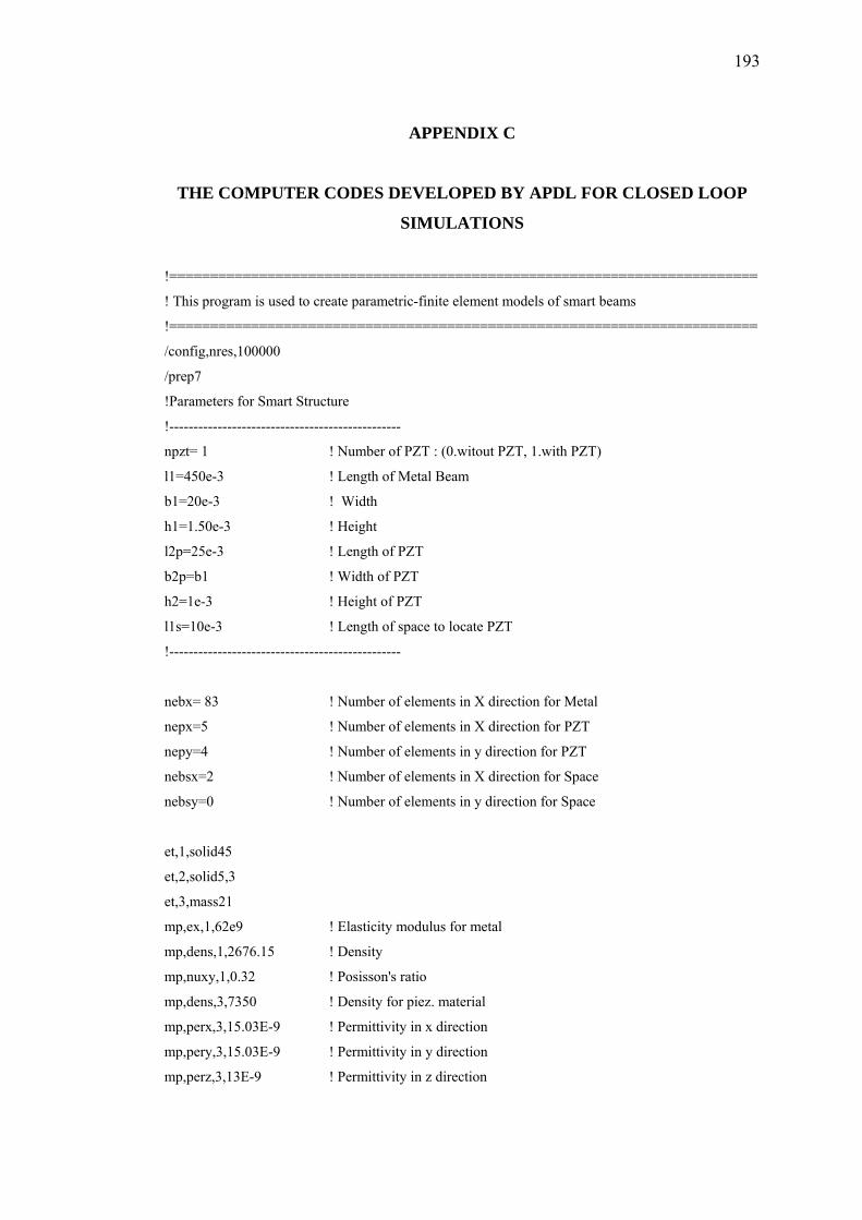
193
APPENDIX C
THE COMPUTER CODES DEVELOPED BY APDL FOR CLOSED LOOP
SIMULATIONS
!========================================================================
! This program is used to create parametric-finite element models of smart beams
!========================================================================
/config,nres,100000
/prep7
!Parameters for Smart Structure
!------------------------------------------------
npzt= 1 ! Number of PZT : (0.witout PZT, 1.with PZT)
l1=450e-3 ! Length of Metal Beam
b1=20e-3 ! Width
h1=1.50e-3 ! Height
l2p=25e-3 ! Length of PZT
b2p=b1 ! Width of PZT
h2=1e-3 ! Height of PZT
l1s=10e-3 ! Length of space to locate PZT
!------------------------------------------------
nebx= 83 ! Number of elements in X direction for Metal
nepx=5 ! Number of elements in X direction for PZT
nepy=4 ! Number of elements in y direction for PZT
nebsx=2 ! Number of elements in X direction for Space
nebsy=0 ! Number of elements in y direction for Space
et,1,solid45
et,2,solid5,3
et,3,mass21
mp,ex,1,62e9 ! Elasticity modulus for metal
mp,dens,1,2676.15 ! Density
mp,nuxy,1,0.32 ! Posisson's ratio
mp,dens,3,7350 ! Density for piez. material
mp,perx,3,15.03E-9 ! Permittivity in x direction
mp,pery,3,15.03E-9 ! Permittivity in y direction
mp,perz,3,13E-9 ! Permittivity in z direction
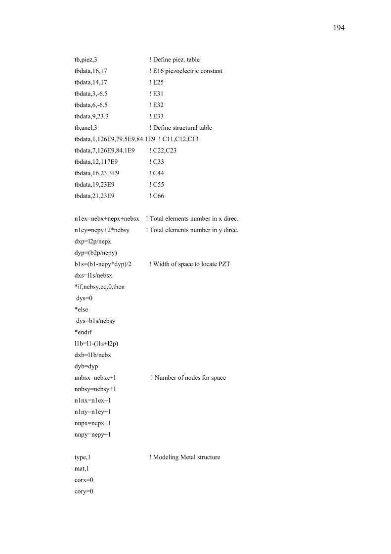
194
tb,piez,3 ! Define piez. table
tbdata,16,17 ! E16 piezoelectric constant
tbdata,14,17 ! E25
tbdata,3,-6.5 ! E31
tbdata,6,-6.5 ! E32
tbdata,9,23.3 ! E33
tb,anel,3 ! Define structural table
tbdata,1,126E9,79.5E9,84.1E9 ! C11,C12,C13
tbdata,7,126E9,84.1E9 ! C22,C23
tbdata,12,117E9 ! C33
tbdata,16,23.3E9 ! C44
tbdata,19,23E9 ! C55
tbdata,21,23E9 ! C66
n1ex=nebx+nepx+nebsx ! Total elements number in x direc.
n1ey=nepy+2*nebsy ! Total elements number in y direc.
dxp=l2p/nepx
dyp=(b2p/nepy)
b1s=(b1-nepy*dyp)/2 ! Width of space to locate PZT
dxs=l1s/nebsx
*if,nebsy,eq,0,then
dys=0
*else
dys=b1s/nebsy
*endif
l1b=l1-(l1s+l2p)
dxb=l1b/nebx
dyb=dyp
nnbsx=nebsx+1 ! Number of nodes for space
nnbsy=nebsy+1
n1nx=n1ex+1
n1ny=n1ey+1
nnpx=nepx+1
nnpy=nepy+1
type,1 ! Modeling Metal structure
mat,1
corx=0
cory=0

195
corz=0
dist=0
*do,ind,1,n1ny
n,ind,corx,cory,corz
*repeat,nnbsx,n1ny,dxs
*if,ind,ge,nnbsy,and,ind,lt,n1ny-nebsy,then
dist=dyp
*else
dist=dys
*endif
cory=cory+dist
*enddo
nodp1=nnbsx*n1ny+1
corx=l1s+dxp
cory=0
corz=0
dist=0
*do,ind,nodp1,nodp1+n1ey
n,ind,corx,cory,corz
*repeat,nepx,n1ny,dxp
*if,ind,ge,nodp1+nebsy,and,ind,lt,nodp1+nebsy+nepy,then
dist=dyp
*else
dist=dys
*endif
cory=cory+dist
*enddo
nodb1=nodp1+nepx*n1ny
corx=l1s+l2p+dxb
cory=0
corz=0
dist=0
*do,ind,nodb1,nodb1+n1ey
n,ind,corx,cory,corz
*repeat,nebx,n1ny,dxb
*if,ind,ge,nodb1+nebsy,and,ind,lt,nodb1+nebsy+nepy,then
dist=dyb

196
*else
dist=dys
*endif
cory=cory+dist
*enddo
nodl=n1nx*n1ny
corx=0
cory=0
corz=h1
dist=0
*do,ind,nodl+1,nodl+n1ny
n,ind,corx,cory,corz
*repeat,nnbsx,n1ny,dxs
*if,ind,ge,nodl+nnbsy,and,ind,lt,nodl+1+nebsy+nepy,then
dist=dyp
*else
dist=dys
*endif
cory=cory+dist
*enddo
nodp2=nodl+nodp1
corx=l1s+dxp
cory=0
corz=h1
dist=0
*do,ind,nodp2,nodp2+n1ey
n,ind,corx,cory,corz
*repeat,nepx,n1ny,dxp
*if,ind,ge,nodp2+nebsy,and,ind,lt,nodp2+nebsy+nepy,then
dist=dyp
*else
dist=dys
*endif
cory=cory+dist
*enddo
nodb2=nodp2+nepx*n1ny

197
corx=l1s+l2p+dxb
cory=0
corz=h1
dist=0
*do,ind,nodb2,nodb2+n1ey
n,ind,corx,cory,corz
*repeat,nebx,n1ny,dxb
*if,ind,ge,nodb2+nebsy,and,ind,lt,nodb2+nebsy+nepy,then
dist=dyb
*else
dist=dys
*endif
cory=cory+dist
*enddo
nodu=2*nodl
en,1,1,n1ny+1,n1ny+2,2,nodl+1,nodl+n1ny+1,nodl+n1ny+2,nodl+2
egen,n1ey,1,1,n1ey
egen,n1ex,n1ny,1,n1ex
nsel,S,LOC,X,(0)
d,all,ux,0
d,all,uy,0
d,all,uz,0
nsel,all
*if,npzt,eq,0,then
*go,:label1
*endif
type,2
mat,3
corx=l1s
cory=nebsy*dys
corz=h1+h2
*do,ind,nodu+1,nodu+nnpy
n,ind,corx,cory,corz
*repeat,nnpx,nnpy,dxp
cory=cory+dyp

198
*enddo
nbs=nodp2+nebsy-n1ny ! Starting coupled node number in Metal
nps=nodu+1 ! Starting node number of PZT
npend=nodu+nnpx*nnpy ! Ending node number of PZT
nes=n1ex*n1ey ! Number of elements in Metal
e1=0
e2=0
e3=0
*do,ind,1,nepx
en,nes+1+e2,nbs+e1,nbs+n1ny+e1,nbs+n1ny+1+e1,nbs+1+e1,nps+e3,nps+nnpy+e3,nps+nnpy+1+e3,
nps+1+e3
*repeat,nepy,1,1,1,1,1,1,1,1,1
e2=e2+nepy
e1=e1+n1ny
e3=e3+nnpy
*enddo
nxinc=nbs
*do,i,1,nnpx
nsel,s,node,,nxinc,nxinc+nepy
nxinc=nxinc+n1ny
cp,1,volt,all
*if,i,eq,1,then
*get,nv0,node,0,num,min
*endif
*enddo
nsel,all
nsel,s,node,,nps,npend
cp,2,volt,all
*get,nv,node,0,num,min
nsel,all
*if,npzt,eq,1,then
*go,:label1
*endif
:label1
finish
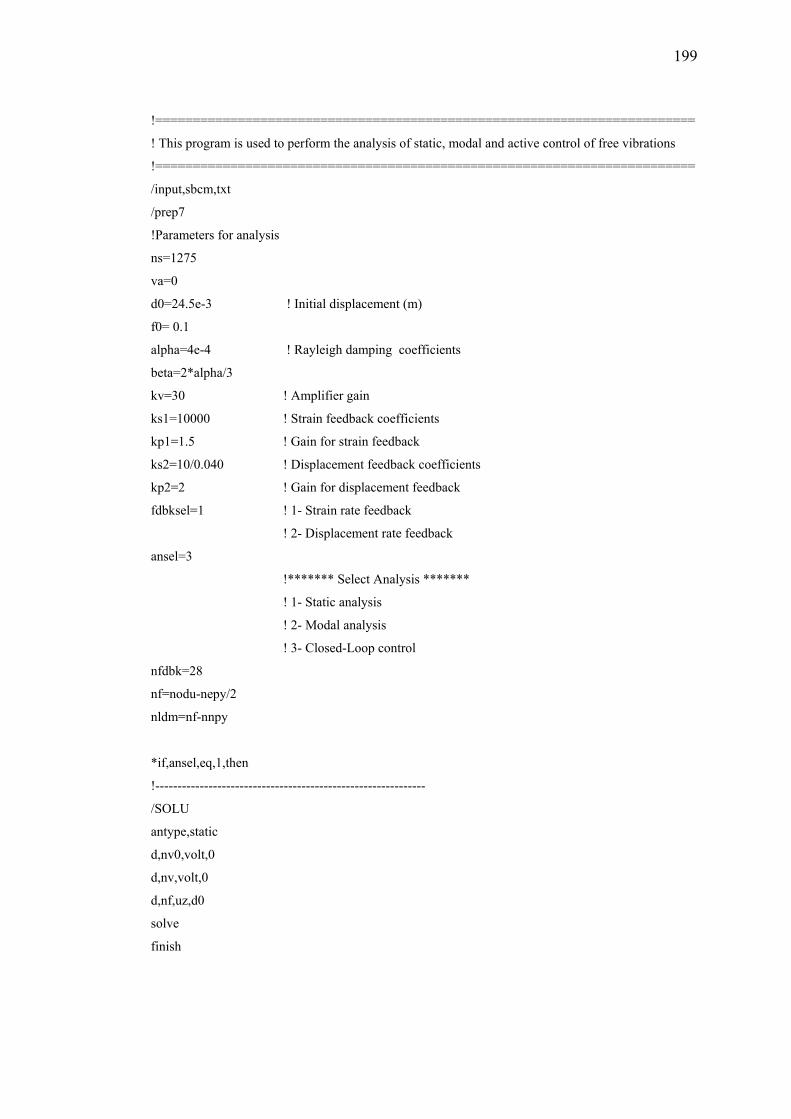
199
!========================================================================
! This program is used to perform the analysis of static, modal and active control of free vibrations
!========================================================================
/input,sbcm,txt
/prep7
!Parameters for analysis
ns=1275
va=0
d0=24.5e-3 ! Initial displacement (m)
f0= 0.1
alpha=4e-4 ! Rayleigh damping coefficients
beta=2*alpha/3
kv=30 ! Amplifier gain
ks1=10000 ! Strain feedback coefficients
kp1=1.5 ! Gain for strain feedback
ks2=10/0.040 ! Displacement feedback coefficients
kp2=2 ! Gain for displacement feedback
fdbksel=1 ! 1- Strain rate feedback
! 2- Displacement rate feedback
ansel=3
!******* Select Analysis *******
! 1- Static analysis
! 2- Modal analysis
! 3- Closed-Loop control
nfdbk=28
nf=nodu-nepy/2
nldm=nf-nnpy
*if,ansel,eq,1,then
!-------------------------------------------------------------
/SOLU
antype,static
d,nv0,volt,0
d,nv,volt,0
d,nf,uz,d0
solve
finish

200
/POST1
PLNSOL,U,Z,1,
*get,Strain,node,nfdbk,epel,x
*get,tipdisp,node,nldm,u,z
finish
*elseif,ansel,eq,2,then
/solu
alphad,alpha
betad,beta
d,nv0,volt,0
d,nv,volt,0
ANTYPE,MODAL,NEW
MODOPT,QRDAMP,5
MXPAND,5
solve
finish
/POST1
SET,LIST
finish
*elseif,ansel,eq,3,then
/solu
d,nv0,volt,0
d,nv,volt,0
ANTYPE,MODAL,NEW
MODOPT,LANB,10
solve
*get,f1,mode,1,freq
finish
dt=1/f1/20
/solu
alphad,alpha
betad,beta
ts=ns*dt
ddele,nv,volt
antype,trans,new
outres,all,all

201
kbc,0
tintp,,0.25,0.5,0.5
timint,on,ALL
trnopt,FULL
deltim,dt
/input,ic24.5,txt
time,dt
solve
vmax=270
ref=0
*do,t,2*dt,ts,dt
*if,fdbksel,eq,1,then
*get,ux1,node,nfdbk,u,x
*get,ux2,node,nfdbk+nnpy,u,x
epsx=(ux2-ux1)/dxp
err=ref-ks1*epsx
va=kp1*kv*err
*elseif,fdbksel,eq,2,then
*get,uztip,node,nldm,u,z
err=ref-ks2*uztip
va=kp2*kv*err
*endif
*if,va,ge,vmax,then
va=vmax
*endif
*if,va,le,-vmax,then
va=-vmax
*endif
d,nv,volt,va
time,t
solve
*enddo
finish
/post26
nsol,2,nldm,u,z,Displacement
nsol,3,nv,volt,,Actuation
plvar,2
*endif
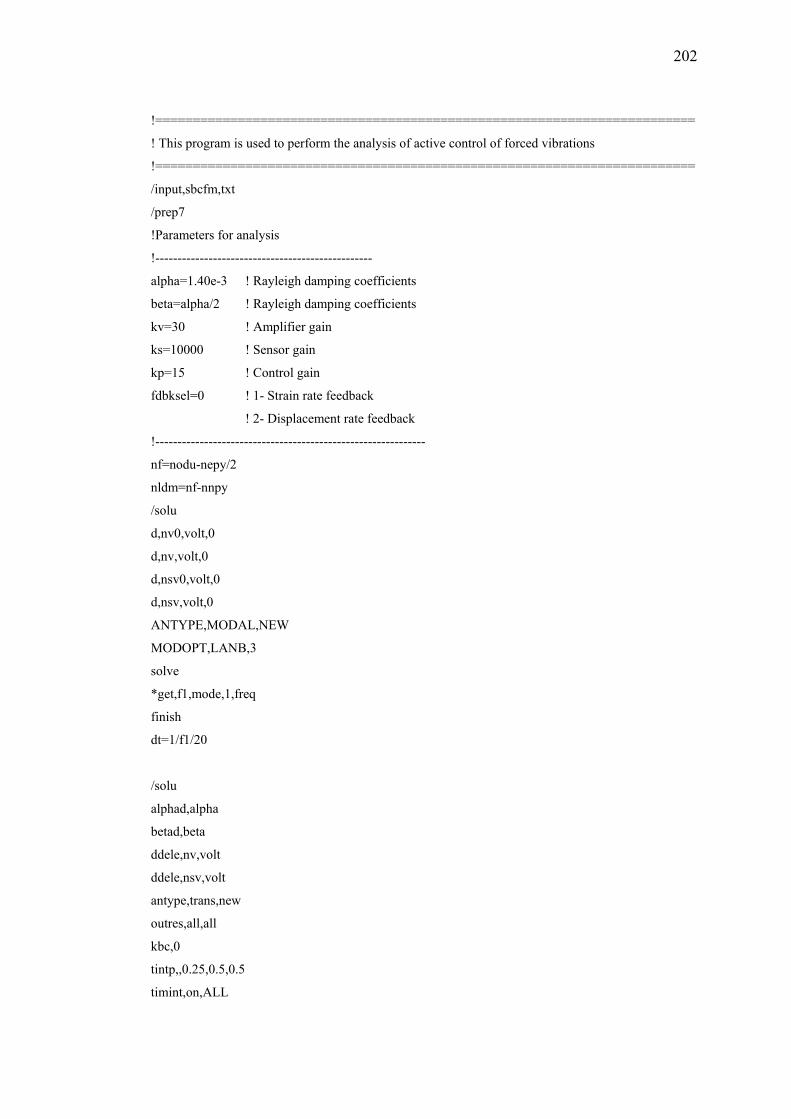
202
!========================================================================
! This program is used to perform the analysis of active control of forced vibrations
!========================================================================
/input,sbcfm,txt
/prep7
!Parameters for analysis
!-------------------------------------------------
alpha=1.40e-3 ! Rayleigh damping coefficients
beta=alpha/2 ! Rayleigh damping coefficients
kv=30 ! Amplifier gain
ks=10000 ! Sensor gain
kp=15 ! Control gain
fdbksel=0 ! 1- Strain rate feedback
! 2- Displacement rate feedback
!-------------------------------------------------------------
nf=nodu-nepy/2
nldm=nf-nnpy
/solu
d,nv0,volt,0
d,nv,volt,0
d,nsv0,volt,0
d,nsv,volt,0
ANTYPE,MODAL,NEW
MODOPT,LANB,3
solve
*get,f1,mode,1,freq
finish
dt=1/f1/20
/solu
alphad,alpha
betad,beta
ddele,nv,volt
ddele,nsv,volt
antype,trans,new
outres,all,all
kbc,0
tintp,,0.25,0.5,0.5
timint,on,ALL

203
trnopt,FULL
deltim,dt
/input,sine,txt
*DIM,vf,,ny
d,nsv,volt,vf(1)
time,dt1
solve
vmax=270
ref=0
*do,i,2,ny
vf(i)=y(i)
d,nsv,volt,vf(i)
*if,fdbksel,eq,1,then
*get,ux1,node,28,u,x
*get,ux2,node,33,u,x
epsx=(ux2-ux1)/dxp
err=ref-ks*epsx
*elseif,fdbksel,eq,2,then
*get,uztip,node,nldm,u,z
vldm=10*uztip/0.040
err=ref-vldm
*endif
va=kp*kv*err
*if,va,ge,vmax,then
va=vmax
*endif
*if,va,le,-vmax,then
va=-vmax
*endif
time,i*dt1
solve
*enddo
finish