1

Integration of HVSR measures and stratigraphic constraints for seismic

microzonation studies: the case of Oliveri (North-Est Sicily)

Di Stefano P.1, Luzio D.

1, Renda P.

1, Martorana R.

1*, Capizzi P.

1,

D’Alessandro A.1, Messina N.

1, Napoli G.

1, Todaro S.

1, Zarcone G.

1

1 Dipartimento di Scienze della Terra e del Mare - DiSTeM, University of Palermo, Italy

* raffaele.martorana@unipa.it

Abstract

Because of its high seismic hazard the urban area of Oliveri has been subject of first level

seismic microzonation. The town develops on a large coastal plain made of mixed fluvial/marine

sediments, overlapping a complexly deformed substrate. In order to identify points on the area

probably suffering relevant site effects and define a preliminary Vs subsurface model for the first

level of microzonation, we performed 23 HVSR measurements. A clustering technique of

continuous signals has been used to optimize the calculation of the HVSR curves. 42 reliable peaks

of the H/V spectra in the frequency range 0.1-20 Hz have been identified. A second clustering

technique has been applied to the set of 42 vectors, containing Cartesian coordinates, central

frequency and amplitude of each peak to identify subsets which can be attributed to continuous

spatial phenomena. The algorithm has identified three main clusters that cover significant parts of

the territory of Oliveri. The HVSR data inversion has been constrained by stratigraphic data of a

borehole. To map the trend of the roof of the seismic bedrock, from the complete set of model

parameters only the depth of the seismic interface that generates peaks fitting those belonging to

two clusters characterized by lower frequency has been extracted.

The reconstructed trend of the top of the seismic bedrock highlights its deepening below the

mouth of the Elicona Torrent, thus suggesting the possible presence of a buried paleo-valley.

1. Introduction

The seismic microzonation of a territory aims to recognize the small scale geological and

geomorphological conditions that may significantly affect the characteristics of the seismic motion,

generating high stress on structures that could produce permanent and critical effects (site effects)

(Ben-Menahem and Singh, 1981; Yuncha and Luzon, 2000). The first phase of the seismic micro-

zoning is the detailed partition of the territory in homogeneous areas with respect to the expected

ground shaking during an earthquake.

The dynamic characteristics of a seismic phase of body or surface waves, generated by an

earthquake and incident on a portion of the ground surface, often show sharp variations, frequency

dependent, sometimes having extremely local character.

Significant increases in amplitude of the phases for which occur peak values of the kinematic

parameters of ground shaking, are called site effects. In general all this phenomena are controlled

by anomalies in the mechanical properties of the shallowest layers of subsoil, when it consists of

soft sediments, or by the shape of surfaces of discontinuity close to or coincident with the

topographic surface.

If we knew a very detailed mechanical model of the cover layer, consisting of soft sediment, we

could predict the site effects or even determine univocally its transfer function by means of

numerical calculation.

The difficulty and costliness of the reconstruction of a suitable model of subsurface using

geophysical techniques and the necessity of not neglecting nonlinear effects (Dimitriu et al., 2000)

have led many researchers to develop and adopt more direct techniques that allow to determine

approximated empirical transfer functions.

2

Nakamura (1989) proposed that in correspondence to the resonance frequencies of a sequence

of layers, the Horizontal to Vertical Spectral Ratio (HVSR) of the seismic noise presents peaks well

correlated with the amplification factor of S waves, generated by earthquakes, between the bottom

and the roof of the stratification.

Not necessarily, however, an HVSR peak must be attributed to resonance frequencies of a

buried structure, it might also depend on characteristics of the sources of noise and in such case it

will be not correlated with amplification effects on incident waves trains.

In fact, one of the most controversial aspects in the application of the HVSR technique

concerns the criteria for the selection, in the microtremor signals, of appropriate time windows for

the calculation of the HVSR curves. However, an appropriate techniques based on an

Agglomerative Hierarchical Clustering (AHC) algorithm may help to discriminate, between peaks

caused by source effects and those due to site effects (D’Alessandro et al., 2013). The separation of

the two effects can allow to determine for each cluster an average HVSR curve better related to the

local site effects and to identify all the significant peaks of the H/V spectra in the chosen frequency

range.

Another problematic aspect must be addressed when the HVSR method is applied for the

seismic microzonation of an area, that is, for its subdivision into relatively uniform areas with

respect to their response to a seismic input. Each HVSR curve may contain more significant peaks

attributable to different causes namely different characteristics of the subsurface.

The cluster analysis can be used to group HVSR peaks probably due to the same site effect, for

example a seismic reflector or a topographic effect.

In each interior point to an area identified by each cluster, it will be reasonable to assume a

same site effect and characterize it in frequency and amplitude with a technique of 2D interpolation

of parameters determined at the measurement points.

Although it is not possible to exclude that the frequencies belonging to the same cluster are due

to different structures or vice versa, the depth values obtained by inverting the average HVSR

curves, if related to peaks of the same cluster, can be interpolated to reconstruct the same seismic

reflector.

2. The study region

2.1. Geological setting

The area of Oliveri is part of the Peloritani Mountains, a segment of the Siculo-Maghrebian

chain that is mainly constituted by a pile of tectonic units consisting of Hercynian metamorphic

rocks and their Meso-Cenozoic sedimentary covers (Giunta et al., 1998, cum biblio).

In the Peloritani Mountains different deformation steps are related to the Alpine orogeny,

superimposed to Hercynian ductile deformations. The Oligo-Miocene contraction has been

characterized by several phases in which there has been the formation of folds associated with

thrust systems that fragmented and stacked the crystalline rocks and their sedimentary covers in

different tectonic units.

Reverse fault systems (breaching) affected the area since the Upper Miocene resulting in

moderate shortening (Giunta & Nigro, 1998). At the end of the Miocene the Tyrrhenian rifting

produced a series of extensional low angle faults that resulted in a thinning of the chain. During

Plio-Pleistocene times the area occupied by the Peloritani Mountains was affected by a strike-slip

tectonic phase that generated two different systems: the first one synthetic with right cinematic and

oriented NO-SE and E-O; the second one antithetical, mainly sinistral and oriented N-S and NE-SW

(Ghisetti & Vezzani, 1977; Nigro & Renda, 2002).

Around the Oliveri plain there is evidence of active tectonics characterizing a right-lateral shear

zone named Aeolian-Tindari-Letojanni fault (Ghisetti, 1979). This fault is generated by two

different geodynamic domains: compressive to west, related to a roughly N-S trusting produced by

continental collision, and extensional to east, controlled by NW-SE expansion of the Calabro-

3

Peloritan Arc (De Guidi et al., 2013). The analysis of seismic and geodetic data, acquired in the last

15 years, and structural and morphological surveys show evidence of tectonic activity in this area to

as recent as the middle-upper Pleistocene (Catalano & Di Stefano, 1997; Ghisetti, 1979; De Guidi et

al., 2013). Recent studies, not far from the Oliveri plain, have characterized some geothermal

springs and gas vents and discussed their possible role in the generation of earthquakes

(Giammanco et al., 2008) and on the basis of paleontological data, have estimated a very high rate

of uplift, up to 5,5 mm/year (Di Stefano et al., 2012).

The lithostratigraphic framework of the substrate of the urban area (Fig. 1) is made up by the

metamorphic basement of the Aspromonte Unit that is covered unconformably by the arenaceus

member of the Capo D’Orlando Flysch. Upwards the flyschoid sediments are tectonically overlaid

by the Argille Scagliose Antisicilide. The previous deposits are capped by sands and calcarenites of

Plio-Pleistocene age. The most recent sediments consists of alluvial and beach deposits.

2.2. Regional Seismicity

The Oliveri territory is located in the area 932 of the ZS9 seismogenic zonation of Italy (Meletti

and Valensise 2004). It includes seismogenic structures largely known through geophysical

exploration. The faults in this area partly allow the retreat of the Calabrian Arc and some are

synthetic faults that segment the Gulf of Patti. The area 932 is one of the areas with the highest

seismic potential of the whole Sicily. In it the earthquake of 1908 occurred, for which different

source mechanisms have been proposed, some of which are, probably, associated with the

activation of complex fault systems or blind faults (Ghisetti 1992; Valensise and Pantosti 1992;

Monaco and Tortorici 1995).

The high rate of seismicity in the Gulf of Patti and in the area between Alicudi and Vulcano is

associated to the two right-slip fault systems, Patti-Volcano-Salina and Sisyphus, respectively

oriented NW-SE and WNW-ESE. The most energetic instrumental earthquakes have occurred in

this area April 15, 1978 and May 28, 1980 with a local magnitude of 5.5 and 5.7 respectively.

The earthquake of 1978 (MW = 6.6), related to movements along these faults (Neri et al.,

1996), caused considerable damage in many countries of the Messina province and was felt up to

the Cosenza province in the north, to Dubrovnik in the south, to Trapani to the west and to the

Ionian coast of Calabria to the east. The estimated maximum macroseismic intensity has been VIII-

IX MCS. Its mean macroseismic intensity in the Oliveri area was VII MCS, where it caused serious

damage in some buildings and significant soil fractures (Barbano et al., 1979).

The earthquakes of Novara di Sicilia, with lower magnitude and shallower hypocenters, seem

to be linked to structures other than the fault system Patti-Volcano-Salina. The earthquakes of Naso

might instead be associated with NE-SW normal faults responsible for the lifting of the chain.

Among the structures present in the southern Tyrrhenian sea, those oriented around EO, would be

responsible for the events of the western sector of the Aeolian Islands, and may have generated

earthquakes like the one in 1823.

Neri et al. (2003) have determined the focal mechanisms of earthquakes with depths less than

50 km, occurred in Calabria and Sicily between 1978 and 2001. These indicate a high heterogeneity

of the deformation field in the area 932. Here the deformation style ranges from extensional with

southwest exposure to compressional with northeast exposure, proceeding from SE to NW.

The first earthquake with a destructive effect in the Oliveri area, reported in the catalogs of

historical Italian seismicity, occurred in March 10, 1786. This seismic event was characterized by

MW = 6.1±0.4, epicenter at Oliveri and MCS intensity equal to IX in the urban area. This

earthquake severely damaged all the cities of the Gulf of Patti in northern Sicily and almost

destroyed the town of Oliveri (Guidoboni et al., 2007).

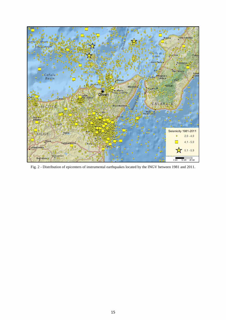
The seismic activity recorded in the last 20 years in the area surrounding the urban center of

Oliveri, represented in Figure 2, is characterized by about 3500 events with local magnitude greater

than 2. Of these about 89% have hypocenters tightly concentrated around an average depth of about

10 km. The remaining 11% consists of events whose hypocenters are thickened around a plane that

4

dips toward the northwest at an angle of about 60° and are distributed rather uniformly with respect

to depths up to 400 km. The sources of these events are located inside the Ionian lithospheric slab

that dips under the Calabrian Arc (Giunta et al., 2004).

An analysis of completeness of these data sets has indicated a local magnitude threshold equal

to about 2.6 (Schorlemmer et al., 2010; D’Alessandro et al., 2011).

The shallow seismic activity has a marked tendency to occur through sequences of aftershocks

sometimes preceded by foreshocks. This tendency was assessed in a quantitative way by comparing

the estimates of the correlation dimension in the domains of the epicenter coordinates and time,

both for the component of the seismicity constituted by events not followed by aftershocks and the

main shock of the sequences that for the total set of events (Adelfio et al., 2006). The estimates of

the space and time correlation dimension relating to independent events are close to those expected

for uniform distributions, as opposed to those for the total set that are much smaller.

The geometric characteristics of the clusters related to the shallower seismicity identify

orientations that are consistent with those of the main tectonic structures of the area.

The seismicity of the last 20 years has also been analyzed in the magnitude domain. For the

events of the area of Figure 2 the value of b of the law of Gutenberg-Richter and the 95%

confidence interval have been estimated, using the estimator of Tinti and Mulargia (1987) not

distorted by the data grouping. In particular, for deeper events, associated with the Ionian slab, the

value of b is equal to 0.6±0.2 while for superficial events the value 1.15±0.13 has been estimated,

which is comparable with the value obtained for the independent component of the seismicity of the

whole south - Tyrrhenian area (see Adelfio et al., 2006).

3. HVSR measurements

3.1. Background and points under discussion

To try to identify areas of the town of Oliveri probably interested in site effects and to define a

preliminary subsurface model 23 HVSR measurements have been performed, quite uniformly

distributed with a mean spacing of about 250 m.

For the measurements the 3 component seismic digital station TROMINO® (Micromed) has

been used, equipped with three velocity transducers.

For each measurement point the recording length was 46 minutes and the sampling frequency

256 Hz. Each recording was subdivided in windows of 50s long. This choice allowed us to have the

minimum number of windows selected for the analysis according to Sesame (2004). Following the

SESAME criteria, the signal relative to each time window was de-trended, baseline corrected,

tapered and band pass filtered between 0.1 and 25 Hz. Than we performed the FFT of each signal

components and determined the HVSR curve following Konno and Ohmachi (1998). The analysis

were limited to the range 0.1-20 Hz, which is the frequency range of interest for seismic

microzonation and earthquake engineering. The data in the frequency domain have been filtered

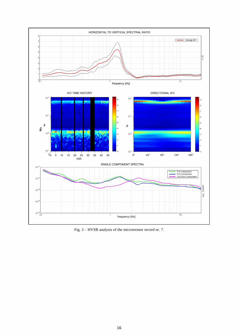
with a triangular window to obtain a smoothing of 10%. The attribution of peaks to resonance

phenomena of buried structures has been validated, in agreement with SESAME criteria, by

analyzing the standard deviation of the spectral amplitudes and the independence from the azimuth

of the mean spectral ratio (Fig. 3). Assuming an approximately one-dimensional ground around

each measurement point, a peak of the HVSR curve should be attributed to characteristics of the

subsoil only if it is azimuthally stable.

In order to obtain reliable HVSR curves, several acquisition and processing criteria must be

adopted. The most important criteria concern the acquisition modes and those of extraction, from a

continuous record, of an optimal set of analysis time windows, for the evaluation of a HVSR

function, dominated by the effects of buried geological structures (SESAME Project, 2004). This

last is probably the most controversial aspect in the HVSR technique implementation. Several

authors believe that spikes and transients in microtremors bring information highly dependent from

the sources and therefore cannot be used to estimate resonance frequencies of sites (Horike et al.,

5

2001; SESAME Project, 2004). Therefore, they exclude the non-stationary portion of the recorded

noise, thus considering only the low-amplitude part of signal, for the computation of the average

HVSR function. Other authors, instead, (Mucciarelli and Gallipoli, 2004) suggest that the non-

stationary large-amplitude noise windows should not be removed, because these, generally, carry

subsoil information that improves the correlation between the noise and earthquakes HVSR curves.

The windows selection can be made in both time and frequency domain. In time domain, the

eligible windows are identified by inspecting the three components of the signal. In frequency

domain the windows are selected, determining the spectral ratios in consecutive time windows, and

subsequently selecting the HVSR curves that, at sight, seem to be more similar to each other.

Clearly, the second approach bypasses the problem of the choice of time windows containing only

the low-amplitude fraction of noise or also high-energy transients. However, the selection of the

windows is still done in an arbitrary way. The use of the visual inspection technique practically

make the processing long and farraginous, the result is strongly dependent by the skill of the

operator, while its reliability is difficult to assess quantitatively.

In a first level seismic microzonation, after the identification for each investigated point of the

peaks of the HVSR curves attributable to resonance effects of the site, it is necessary to delineate

areas of similar behaviour in seismic perspective. The identification of these areas involves the

simultaneous assessment of several parameters such as the frequency and amplitude of the

resonance frequencies, and the positions and the mutual distances between the measuring points.

The task becomes particularly difficult when it is possible to identify on the HVSR curves different

peaks associable with different resonance frequencies of the investigated site.

To overcome the aforementioned problems, we have implemented two automatic procedures

based on cluster analysis.

3.2. Implementation by cluster analysis

Cluster analysis is the task of grouping a set of objects in such a way that objects in the same

group (called cluster) are, in some sense, more similar to each other (internal cohesion), than to

those in other groups (external isolation). It is a main task of exploratory data mining, and a

common technique for statistical data analysis.

Clustering is, typically, an unsupervised process and the results of the application of different

algorithms to the same data set, may be very different from each other, thus the assessment of the

clustering algorithms is fundamental. Several clustering validation approaches have been developed

(Gan et al., 2007; Everit, et al., 2011), mainly based on the concepts of homogeneity and separation.

We used as measure of cluster quality the variance decomposition method using the within-class

and the between-classes variances as measure of homogeneity and separation, respectively (Gan et

al., 2007; Everit, et al., 2011). A good clustering should identify a small number of clusters

characterized by a within-class variance less than of the between-classes one. Both the procedure

proposed are based on the Hierarchical Clustering (HC) Algorithms (Gan et al., 2007; Everit, et al.,

2011). The HC algorithms are explorative methods for which it is not necessary to fix a priori the

number of clusters. HC methods work with a measure of proximity between objects to be clustered.

The proximity measure has to be chosen, so that it is suited to the nature of the data.

Hierarchical clustering algorithms can be agglomerative or divisive. In the Agglomerative

Hierarchical Clustering (AHC), or bottom-up approach, each object begins the process as the only

member of its own cluster and the process is concluded with the inclusion of all the objects in a

single cluster; in the Divisive Hierarchical Clustering (DHC), or top-down approach, instead, all

observations are initially placed in a single cluster, which is subdivided iteratively until to obtain N

clusters. Application of both AHC and DHC verifies that the two algorithms leads to very similar

solutions, but the first kind of processing is less time-consuming.

To address the two problems above described both the implemented procedures are based on

the AHC algorithm and used the Average Linkage (AL) criterion, in which the dissimilarity

between the objects A and B is the average of the dissimilarities between the objects of A and the

6

objects of B (Gan et al., 2007; Everit, et al., 2011). This has been chosen because, besides providing

a fair representation of the data space properties, in our tests the best results in terms of variance

decomposition and stability of the solutions were obtained.

Several measure of proximity between two elements of the set were proposed in literature to

measure the similarity/dissimilarity of different kinds of objects (Gan et al., 2007; Everit, et al.,

2011). Clearly, the choice of the type of proximity measure must respect specific criteria and should

be optimized depending on the type of data and aim of clustering (Gan et al., 2007; Everit, et al.,

2011).

For the identification of the optimal set of analysis windows for the determination of the

average HVSR curve, we have adopted as a measure of proximity the Standard Correlation ( )

defined as:

∑

√∑

∑

were and indicate the values of the spectral ratios relative to the i-th frequency and the generic

pair of analysis time windows x and y. It takes into account both the position and amplitude of the

peaks present on the HVSR curves.

To define clusters of HVSR peaks, representative of measurement points, with the aim of

defining homogeneous areas in seismic perspective, it is important that the process of clustering

takes into account all the parameters involved; these are clearly the period and the amplitude of

each peak. In addition to these parameters, we could consider also the values of the same

parameters in the neighbouring points. For this reasons, in the implemented clustering procedure,

we have defined the following proximity measure:

( )

where , and are normalized Euclidean distance in the parameters space (period, amplitude

and measurement position, respectively) and , and are weights to be assigned to the respective

distances. These parameters are reported in Table 1. The results of the analysis carried out are

summarized in dendrograms and the variance decomposition was adopted as optimal criterion for

the choice of the proximity cut levels.

4. Frequency maps

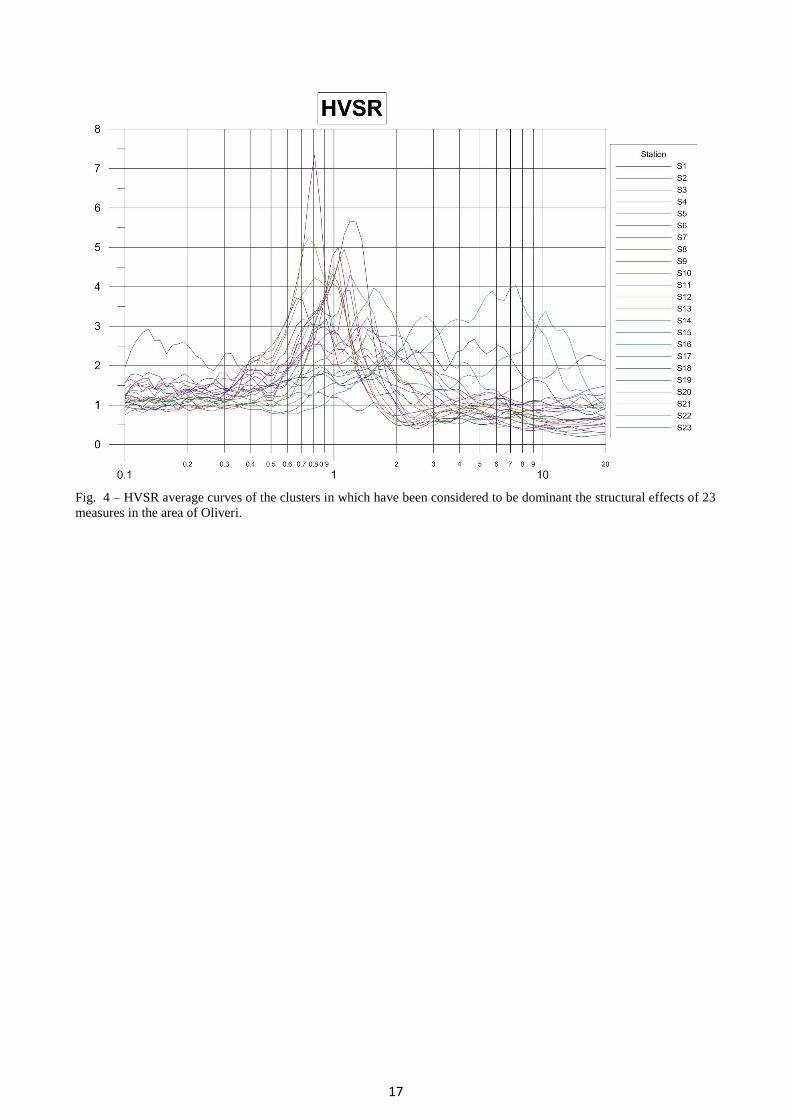
The HVSR data (Fig. 4) have revealed the likely presence of amplification of ground motion in

the frequency range 0.7÷1.6 Hz, over a large part of the urban area. The thickness of the soft

coverage in few places where it is known and its lithological composition allow us to hypothesize

that the cause of amplification is the resonance of the same coverage.

The clustering procedure used to group peaks of HVSR average curves related to different

sites, has allowed to identify areas characterized by site effects probably caused by the same buried

structure. Considering the parameters of such peaks as sampling of spatial trends that are

continuous on the area containing the measuring points, it is possible to estimate the expected peak

amplitude and frequency at each point of the area by two-dimensional interpolation techniques.

In the cluster algorithm the elements of the similarity matrix are weighted averages of

Euclidean relative distances between the quantitative parameters of a pair of peaks, and each

difference between pairs of parameters is normalized by the maximum difference in the sample. To

avoid the inclusion in the same cluster of more peaks relative to the same measurement point, the

normalized relative distance of coincident points was placed equal to 1. The choice of the weights to be assigned to the equation (2) should be made on the basis of

the statistical parameters that allow to quantify the goodness of the clustering procedure, such as

7

homogeneity and separation of the clusters, but also on the basis of importance and reliability of

each parameter.

The resonance period of a site is a very important parameter and surely the most robust one

that can be estimated from the HVSR curve. The resonance period is linked to the local geology in

term of S-wave velocity and thickness of the resonant layer. On the other hand, the associated

amplitude value is not a robust parameter. In fact, only if the microtremors wave-field consist of

body waves the shape of the HVSR curves is mainly controlled by the S-wave transfer of the

shallowest sedimentary layers and the peaks amplitude may be straightforward related to subsoil

amplification factors. The topographical distance is instead a parameter of high importance, both for

the identification of homogeneous areas in seismic perspective, but also as an indirect measure of

the reliability of peaks of the HVSR curves associated to resonance effects.

In order to identify the optimal weights values in our clustering procedure we have tried to

cluster our data using all the possible combinations of weights ranging between 0.2 and 0.5, with

step of 0.1. The values of weights able to provide the best result in term of variance decomposition

(minimum within-class and maximum between-classes variance) were the following: =0.4, =0.2

and =0.4.

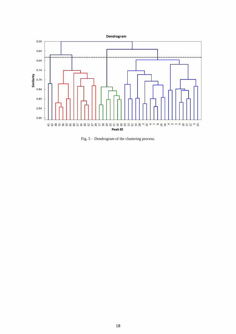
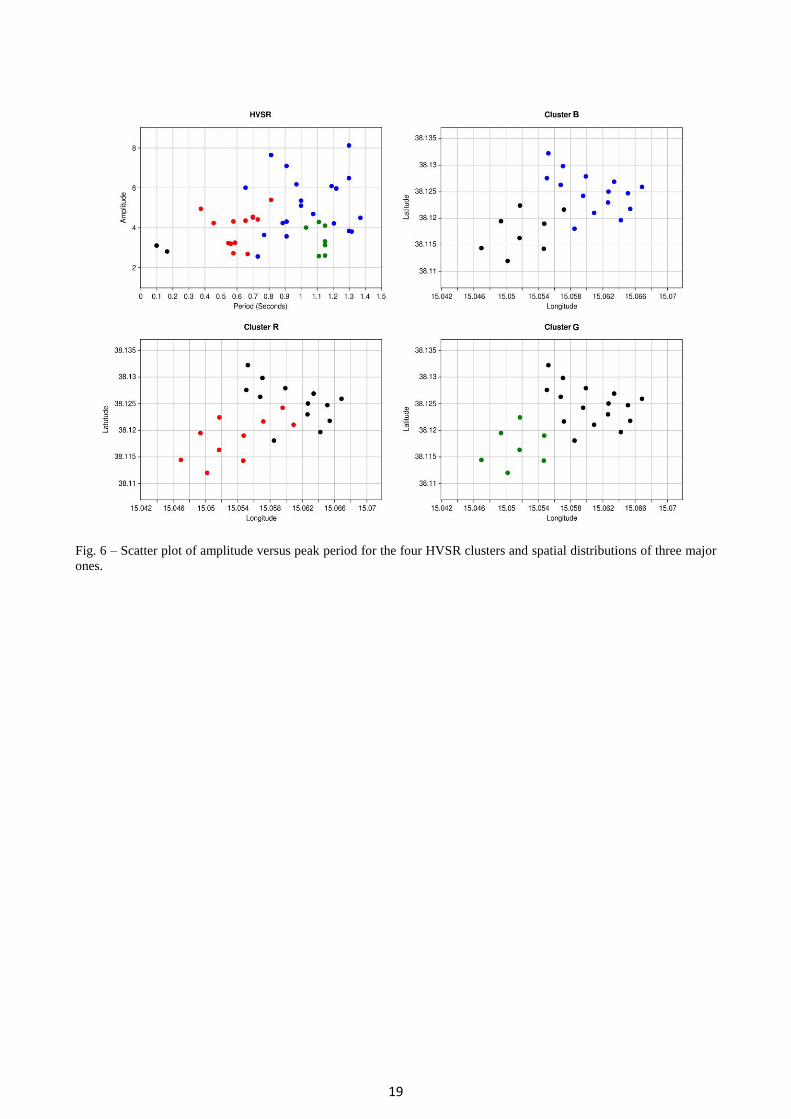
The procedure of clustering made it possible to split the total set of peaks in four clusters

referred to as: B (Blue), R (Red), G (Green), V (Violet), respectively, consisting of 21, 12, 7, and 2

peaks. The cluster made up of only two peaks has been neglected in the overall description of the

area due to poor reliability of both peaks, highlighted by the parameters listed in Tab. 1. Fig 5

shows the dendrogram of the clustering process. From this it is clear that, adopting a cut threshold

slightly lower than the optimal one adopted by the calculation code, the three remaining clusters

would be gathered in a single cluster. Different criteria can be used to find the optimal threshold. In

this paper, the optimal threshold was identified seeking in the dendrogram the large gap between

two successive levels of the hierarchy.

Fig. 6 shows the characteristics of the clusters in the diagram H/V vs. period and the spatial

distribution of B, R and G clusters.

As the two clusters B and G are very near in the scatter plot and their areas have an empty

intersection, it was considered reasonable to assume that they represent the effects, continuously

variable on the union of their areas, of a single source phenomenon. In particular it is assumed that

B and G are related to the resonance effect of a covering layer delimited at its base by the same

discontinuity surface with variable depth. Conversely it is assumed that the cluster R, whose extent

represent a significant part of that of BG and is characterized by higher frequencies respect to the

corresponding ones of the peaks of BG, show the resonance effects of the sedimentary cover

down to a shallower interface.

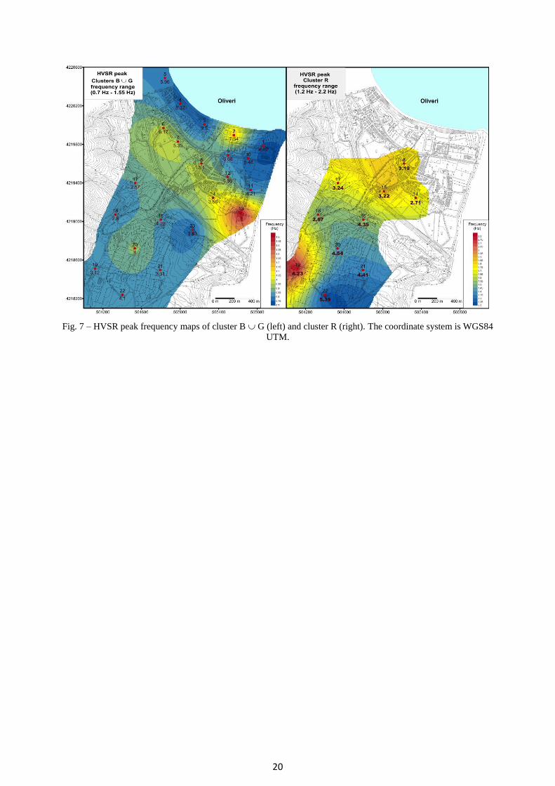
Therefore, two different maps can be reconstructed, each of them grouping and separately

representing the continuous trend of the frequency for the clusters ABG and R. The

amplification estimated at the measurement points is reported numerically in the maps, being not

reliably mappable with smoothed trends over large areas.

For the processing of the maps, the kriging algorithm has been applied to interpolate the

experimental peak frequencies at the nodes of a regular lattice with spacing equal to 10 m. The

frequency maps are plotted using a contour equidistance equal to 0.05 (Fig. 7).

An area south of the town, interesting for the spatial planning, seems to be characterized by

higher amplification at frequencies greater than 1.2 Hz (Fig. 7, right).

5. Bedrock mapping by inversion of HVSR measurements

8

The determination of the parameters that characterize the subsoil from the H/V curves provides

unreliable results if you don’t use an initial model already representative of the real geological

stratification, well constrained by drilling data, geological observations or results of other

geophysical surveys.

It should be, also, pointed out that, due to lateral variations of geologic parameters as: porosity,

water content, fracturing degree, etc. the mechanical parameters of each layer will not be uniformly

distributed with obvious negative consequences on the accuracy of the estimate of the depth of

geological interfaces and in particular the roof of the seismic bedrock.

Taking into account the available geological information, the H/V curves have been inverted to

estimate the depth of the seismic bedrock, also reported in Table 1.

The inversion has been carried out using the Dinver inversion code, developed in the frame of

the project Geopsy (Wathelet et al., 2004; Wathelet 2008). In this technique the computation of the

dispersion curve for a stack of horizontal and homogeneous layers is determined (Haskell, 1953).

Only the Rayleigh phase velocities are considered as the experimental dispersion curve is generally

obtained from processing the vertical components of noise. A limit of this method lies in the

uncertain composition of seismic noise and in the impossibility to include among the unknown

parameters those relating to the model of the microseismic field (Peterson, 1993). For the inversion

the neighbourhood algorithm (Sambridge 1999) was used. This is a stochastic direct-search method

for finding models of acceptable data fit inside a multidimensional parameter space.

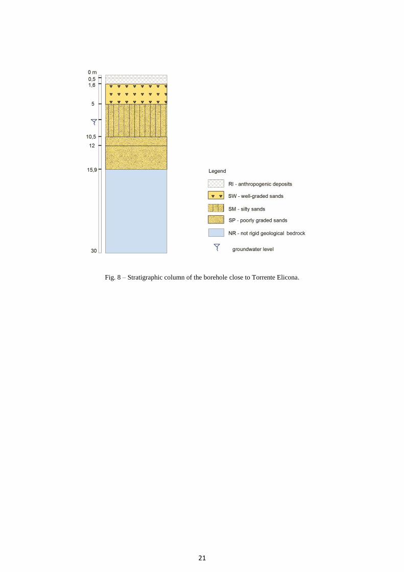
Unfortunately, it has been possible to constrain the model using only the data of a single

borehole, located at the eastern boundary of the municipality (fig. 8), to impose constraints on the

thicknesses of the layers in the inversion of the HVSR curve related to the nearest recording point.

We considered reliable inverse models with misfits about equal or less than 1. Misfits were

calculated as a sum of squared differences between observed data and calculated ones, normalized

by the variance.

To define the starting model for the inversion, the values of shear-wave velocity of the cover

available for the studied area were used. In particular, we considered about 200 to 250 m/s for

alluvium and about 350 to 400 m/s in correspondence of silty sands.

The depth of transition of the shear wave velocity from less to greater than 800 m/s is

considered the depth of the seismic bedrock. When evaluating the reliability of the estimate of this

depth, we must consider that the trends represented are heavily influenced by the interpolation

process between the HVSR measuring points. The depth values obtained from every measuring

points are in fact only possible estimates, assuming minimal lateral variations. To avoid

interpolation between depths of interfaces due to different geological structures, it was decided to

group and correlate frequencies related to the same cluster. However it is not possible to exclude

that frequencies belonging to the same cluster are due to different structures or vice versa.

In almost all the HVSR measurements carried out on the alluvial material a maximum peak is

mostly evident in the range 0.7 - 1.4 Hz (Fig. 4). This, by the inversions results, seems to be related

to a variation of the shear-wave velocities that, under a depth of 40-60 meters reach values

attributable to a seismic bedrock (about 800 m/s).

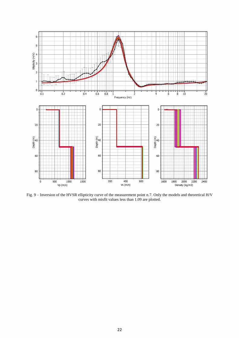
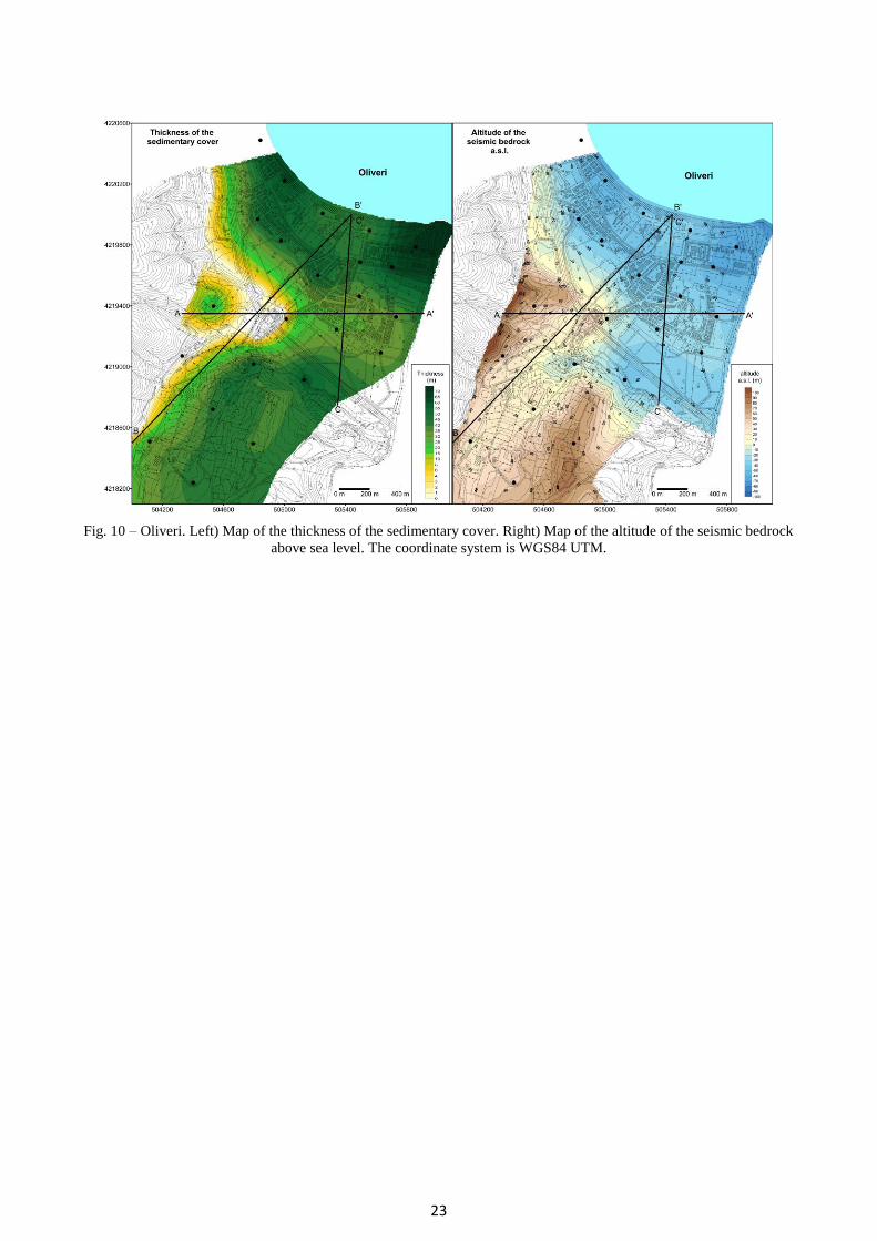
Analyzing the 1D inverse models (fig. 9) derived by inverting HVSR measurements, estimates

of the depth of the seismic bedrock have been obtained. These, together with other reliable data like

drilling and other geophysical surveys, were used to construct the map of the thickness of the

sedimentary cover (Fig. 10, left) and the map of the altitude of the top of seismic bedrock above sea

level (Fig. 10, right). The estimates of the depth of the bedrock were interpolated by imposing a

constraint of a depth equal to zero in areas where geological strata with elastic characteristics of

seismic bedrock outcrop. The kriging interpolation algorithm was used, obtaining a lattice with

equidistance between nodes equal to 10 m.

The map of the bedrock depth contours was obtained by extracting from the Digital Elevation

Model of the area a grid of points equidistant 50 m. From these the corresponding lattice of the

depth of the bedrock were subtracted. This choice was made in order to obtain a trend of the

9

isobaths that was not excessively tied to topographic detail but which, however, did not present

unrealistic areas with higher elevations of the topographic surface. It should however emphasize

that the real detail of the maps can't be higher than the sampling density of the HVSR

measurements, which generally is not less than 300 m.

6. Geological interpretation

Considering the geological configuration of the subsoil and the values of shear-wave velocity a

preliminary identification was made of the geological structures that can cause seismic resonance.

It was not possible to define the lithological distribution in particular under the town, for the

lack of well data. Only the data from two wells have been used; the first is located close to Torrente

Elicona (Fig. 8), the second is located close to the Castello hill. The analysis of the core of the first

one shows the presence of anthropic deposits in the first 1.6 m, followed by 3.4 m of well graded

sand with gravel elements of metamorphic origin, 5.5 m of silty sand, with rare rounded gravel

elements, and 5.4 m of poorly graded sand. The altered substrate, according to its mechanical

characterization by HVSR data, seems to be made by incoherent sand and grey silt. The analysis of

core samples permitted to recognize bivalve fauna. The groundwater level is placed at a depth of 7.5

m.

The core relative to the second well shows evidence of a tectonic dislocation that put in contact

the “Argille Scagliose” unit with the metamorphic basement. In the northern side of Torrente

Castello, the flyschoid cover has a thickness of about 20 m while, in the southern part, the

thicknesses of clay and calcarenite covers exceed 45 m (Fig.10). The nature of the covers is related

to the sedimentary contribution of the rivers and sea level fluctuations.

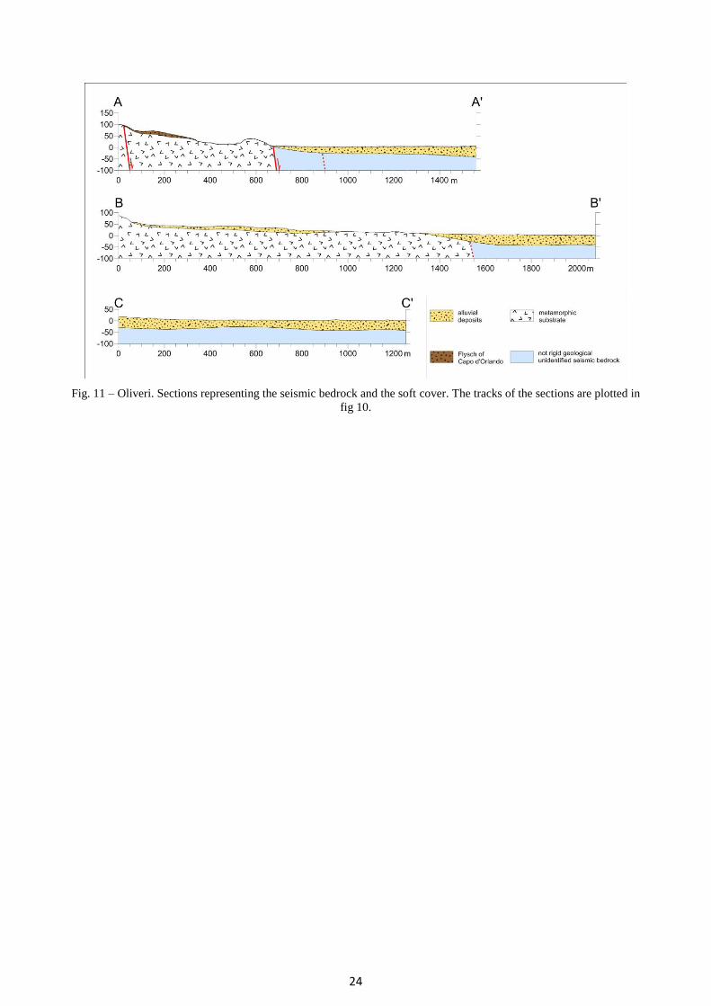
On the basis of the 3D trend of seismic bedrock and of geological information from field

surveys and from published geological maps, three geological sections were drawn (fig. 11).

In the section A, oriented from west to east, it is possible to observe, in the westernmost part,

the stratigraphic overlay of the Flysch of Capo D'Orlando on the metamorphic substrate, which is

lowered eastward by normal faults. The alluvial deposits of coastal plain are onlapping on the

substrate whose lithology is not known in most of the area (sections B and C in fig. 11) due to the

lack of information deriving from deep boreholes. Therefore the only information is related to

geophysical analysis. Finally, along the Oliveri plain some catalogs (e.g. ITHACA) and structural

studies (Ghisetti & Vezzani, 1977) testify the presence of an active fault that in geological sections

is approximately shown.

The reconstructed model suggest the presence of two buried river bed separated by a relief. The

sediment thickness in these two areas is about 45 m. In the seismic bedrock map (Fig. 10, right) is

possible to observe as the rivers bed suffer a migration toward the present day position. According

to the bedrock map the relief that separates the two depressions has a depth of 40 m while the floor

of basins show a depth of 60-70 m. In the southern part of the town there is another basin in which

the bedrock has a deepness of 40 m. This could be related to another minor river joined with

Torrente Elicona. Based on hydrogeological information the presence of groundwater level in the

floodplain is attested at a depth less than 15 m. This condition renders the floodplain exposed to

liquefaction risk.

7. Conclusions

The application of a first clustering procedure to the set of HVSR data allowed to separate in

different clusters the noise windows with spectral effects due to subsurface structures and those

dominated by accidental interference effects between waves trains of a different nature.

The average spectral ratio of the cluster dominated by structural effects, often has been

characterized by smaller variance of the frequencies and amplitudes of the significant peaks,

compared to those of the peaks determined with standard methods.

10

A second clustering procedure applied to estimated frequencies and amplitudes of the peaks,

allowed to identify areas where it could be considered realistic to interpolate the peak parameters

linked to the same buried structures.

Assuming that the three main identified clusters contain peaks produced by resonance effects of

layers with varying thickness, the possible trend of the roof of the seismic bedrock was

reconstructed by inversion of the HVSR curves constrained with geological and lithological

information and considering a minimum lateral variability of the physical and geometrical

parameters. The reliability of the 3D model obtained is limited by the lack of geophysical and

drilling data, which would have allowed us to better constrain the values of the unknown parameters

of the model. However, the general characteristics of the reconstructed subsoil are fully compatible

with the geological model of the area. The necessary surveys to increase the resolution and

reliability of the model will be carried out in more detailed studies provided by the microzoning of

second and third level.

11

References

Adelfio, G., Chiodi, M., De Luca, L., Luzio, D., and Vitale, M.: Southern-Tyrrhenian seismicity in space-time-

magnitude domain, Annals of Geophysics, 49 (6), pp. 1245-1257, 2006

Barbano, M.S., Bottari, A., Carveni, P., Cosentino, M., Federico, B., Fonte, G., Lo Giudice, E., Lombardo, G., and

Patanè, G.: Macroseismc study of the gulf of Patti earthquake in the geostructural frame of the North-Eastern Sicily,

Bollettino della Società Geologica Italiana, 98, 155-174, 1979.

Ben-Menahem, A. and Singh, S.J.: Seismic Waves and Sources, Springer-Verlag, New York, 1981.

Catalano, S. and Di Stefano, A.: Sollevamenti e tettogenesi pleistocenica lungo il margine tirrenico dei Monti

Peloritani: integrazione dei dati geomorfologici, strutturali e biostratigrafici, Il Quaternario (Italian Journal of

Quaternary Sciences) 10 (2), 337–342, 1997.

D'Alessandro, A., Capizzi, P., Luzio, D., Martorana, R., and Messina, N.: Improvement of HVSR technique by cluster

analysis. Geoitalia 2013, IX FIST, Pisa, 16-18 Settembre 2013, 2013.

D’Alessandro, A., Luzio, D., D’Anna, G., and Mangano, G.: Seismic Network Evaluation through Simulation: An

Application to the Italian National Seismic Network, Bulletin of the Seismological Society of America, DOI:

10.1785/0120100066, 101 (3), 1213-1232, 2011.

De Guidi, G., Lanzafame, G., Palano, M., Puglisi, G., Scaltrito, A., and Scarfì, L.: Multidisciplinary study of the Tindari

Fault (Sicily, Italy) separating ongoing contractional and extensional compartments along the active Africa-Eurasia

convergent boundary, Tectonophysics, 588, 1-17, 2013.

Di Stefano, E., Agate, M., Incarbona, A., Russo, F., Sprovieri, R., and Bonomo, S.: Late Quaternary high uplift rates in

northeastern Sicily: evidence from calcareous nannofossils and benthic and planktonic foraminifera, Facies, 58,

issue 1, 1-15, 2012.

Dimitriu, P., Theodulidis, N., and Bard, P.Y.: Evidence of non linear site in HVSR from SMART1 (Taiwan) data, Soil

Dynamicsand Earthquake Engineering, 20, 155-165, 2000.

Ghisetti, F.: Relazioni tra strutture e fasi trascorrenti e distensive lungo i sistemi Messina-Fiumefreddo, Tindari-

Letojanni e Alia-Malvagna (Sicilia nord-orientale): uno studio microtettonico. Geol. Rom., 18, 23-58, 1979.

Ghisetti, F.: Fault parameters in the Messina Strait (southern Italy) and relations with the seismogenic source,

Tectonophysics, 210 (1-2), 117-133, 1992.

Ghisetti, F. and Vezzani, L.: Evidenze di linee di dislocazione sul versante meridionale dei Monti Nebrodi e Madonie e

loro significato neotettonico, Boll. Geodesia e Sc. affini, 36 (4): 411-437, 1977.

Giammanco, S., Palano, M., Scaltrito, A., Scarfì, L., and Sortino, F.: Possible role of fluid overpressure in the

generation of earthquake swarms in active tectonic areas: the case of the Peloritani Mts. (Sicily, Italy), Journal of

Volcanology and Geothermal Research 178, 795–806, 2008.

Giunta, G., Messina, A., Bonardi, G., Nigro, F., Somma, R., Cutrupia, D., Giorgianni, A., and Sparacino, V.: Geologia

dei Monti Peloritani (Sicilia NE), Guida all’escursione, 77° Riunione estiva, Palermo, 1998.

Giunta, G. and Nigro, F.: Some tectono-sedimentary constraints to Oligo-Miocene evolution of the Peloritani Thrust

Belt, Tectonophysics, 315: 287-299, 1998.

Giunta, G., Luzio, D., Tondi, E., De Luca, L., Giorgianni, A., D'Anna, G., Renda, P., Cello, G., Nigro, F., and Vitale,

M.: The Palermo (Sicily) seismic cluster of September 2002, in the seismotectonic framework of the Tyrrhenian Sea-

Sicily border area,. Annals of Geophysics, 47 (6), 1755-1770, 2004.

Guidoboni, E., Ferrari, G., Mariotti, D., Comastri, A., Tarabusi, G., and Valensise, G.: Catalogue of Strong

Earthquakes in Italy (CFTI), 461 B.C. - 1997 and Mediterranean Area 760 B.C. - 1500,

http://storing.ingv.it/cfti4med/, 2007.

Horike, M., Zhao, B., and Kawase, H.: Comparison of site response characteristics inferred from microtremors and

earthquake shear waves, Bulletin of the Seismological Society of America, 91 (6), 1526-1536, 2001.

Konno, K. and Ohmachi, T.: Ground-Motion Characteristics Estimated from Spectral Ratio between Horizontal and

Vertical Components of Microtremor, Bull. Seism. Soc. Am., 88:1, 228-241, 1998.

Meletti, C. and Valensise, G.: Zonazione sismo genetica ZS9 – App.2 al Rapporto Conclusivo,

http://zonesismiche.mi.ingv.it/documenti/App2.pdf, 2004.

Monaco, C. and Tortorici, L.: Tectonic role of ophiolite-bearing terranes in the development of the southern Apennines

orogenic belt, Terra Nova, 7 (2), 153-160, 1995.

Mucciarelli, M. and Gallipoli, M.R.: The HVSR technique from microtremor to strong motion: empirical and statistical

considerations, 13th World Conference on Earthquake Engineering. Vancouver, B.C., Canada. August 1-6, 2004.

45, 2004.

Nakamura, Y.: A Method for Dynamic Characteristics Estimation of Subsurface using Microtremor on the Ground

Surface, Quarterly Report of Railway Technical Research Institute (RTRI), 30, 1., 1989.

Neri, G., Caccamo, D., Cocina, O., and Montalto, A.: Geodynamic implications of earthquake data in the southern

Tyrrhenian sea, Tectonophysics, 258 (1-4), 233-249, 1996.

Neri, G., Barberi, G., Orecchio, B., and Mostaccio, A.: Seismic strain and seismogenic stress regimes in the crust of the

southern Tyrrhenian region, Earth and Planetary Science Letters, 213 (1-2), 97-112, 2003.

Nigro, F. and Renda, P.: Forced mode dictated by foreland fault-indenter shape during oblique convergence: the

Western Sicily mainland, Boll. Soc. Geol. It., 121, 151-162, 2002.

12

Peterson, J.: Observations and modeling of seismic background noise, Open-File Report, 93-322, US Geological

Survey, Albuquerque, NM., 1993.

Sambridge, M.: Geophysical inversion with a neighbourhood algorithm - I. Searching a parameter space, Geophysical

Journal International 103, 4839–4878, 1999.

Schorlemmer, D., Mele, F., and Marzocchi, W.: A completeness analysis of the National Seismic Network of Italy, J.

Geophys. Res. 115, B04308, doi 10.1029/2008JB006097, 2010.

SESAME Project: Guidelines for the implementation of the H/V spectral ratio technique on ambient vibrations.

Measurements, processing and interpretation, WP12, deliverable no. D23.12, http://sesame-fp5.obs.ujf-

grenoble.fr/Papers/HV_User_Guidelines.pdf, (2004).

Tinti, S. and Mulargia, F.: Confidence intervals of bvalues for grouped magnitudes, Bull. Seismol. Soc. Am., 77, 2125-

2134, 1987.

Valensise, G. and Pantosti, D.: A 125 Kyr-long geological record of seismic source repeatability: the Messina Straits

(southern Italy) and the 1908 earthquake (Ms 7 1/2 ),. Terra Nova, 4 (4), 472-483, 1992.

Wathelet, M.: An improved neighborhood algorithm: Parameter conditions and dynamic scaling, Geophysical Research

Letters, 35 (9), art. no. L09301, 2008.

Wathelet M., Jongmans D., and Ohrnberger M.:Surface-wave inversion using a direct search algorithm and its

application to ambient vibration measurements, Near Surface Geophysics, 211-221, 2004.

Yuncha, Z.A. and Luzon, F.: On the horizontal-to-vertical spectral ratio in sedimentary basins. Bulletin of the

Seismological Society of America. 90, 4, 1101-1106, 2000.

13

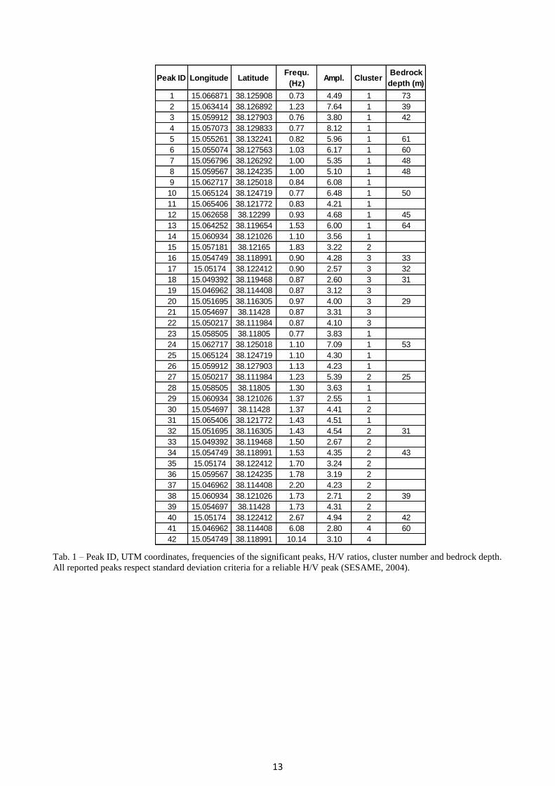
Tab. 1 – Peak ID, UTM coordinates, frequencies of the significant peaks, H/V ratios, cluster number and bedrock depth.

All reported peaks respect standard deviation criteria for a reliable H/V peak (SESAME, 2004).

Peak ID Longitude LatitudeFrequ.

(Hz)Ampl. Cluster

Bedrock

depth (m)

1 15.066871 38.125908 0.73 4.49 1 73

2 15.063414 38.126892 1.23 7.64 1 39

3 15.059912 38.127903 0.76 3.80 1 42

4 15.057073 38.129833 0.77 8.12 1

5 15.055261 38.132241 0.82 5.96 1 61

6 15.055074 38.127563 1.03 6.17 1 60

7 15.056796 38.126292 1.00 5.35 1 48

8 15.059567 38.124235 1.00 5.10 1 48

9 15.062717 38.125018 0.84 6.08 1

10 15.065124 38.124719 0.77 6.48 1 50

11 15.065406 38.121772 0.83 4.21 1

12 15.062658 38.12299 0.93 4.68 1 45

13 15.064252 38.119654 1.53 6.00 1 64

14 15.060934 38.121026 1.10 3.56 1

15 15.057181 38.12165 1.83 3.22 2

16 15.054749 38.118991 0.90 4.28 3 33

17 15.05174 38.122412 0.90 2.57 3 32

18 15.049392 38.119468 0.87 2.60 3 31

19 15.046962 38.114408 0.87 3.12 3

20 15.051695 38.116305 0.97 4.00 3 29

21 15.054697 38.11428 0.87 3.31 3

22 15.050217 38.111984 0.87 4.10 3

23 15.058505 38.11805 0.77 3.83 1

24 15.062717 38.125018 1.10 7.09 1 53

25 15.065124 38.124719 1.10 4.30 1

26 15.059912 38.127903 1.13 4.23 1

27 15.050217 38.111984 1.23 5.39 2 25

28 15.058505 38.11805 1.30 3.63 1

29 15.060934 38.121026 1.37 2.55 1

30 15.054697 38.11428 1.37 4.41 2

31 15.065406 38.121772 1.43 4.51 1

32 15.051695 38.116305 1.43 4.54 2 31

33 15.049392 38.119468 1.50 2.67 2

34 15.054749 38.118991 1.53 4.35 2 43

35 15.05174 38.122412 1.70 3.24 2

36 15.059567 38.124235 1.78 3.19 2

37 15.046962 38.114408 2.20 4.23 2

38 15.060934 38.121026 1.73 2.71 2 39

39 15.054697 38.11428 1.73 4.31 2

40 15.05174 38.122412 2.67 4.94 2 42

41 15.046962 38.114408 6.08 2.80 4 60

42 15.054749 38.118991 10.14 3.10 4

14

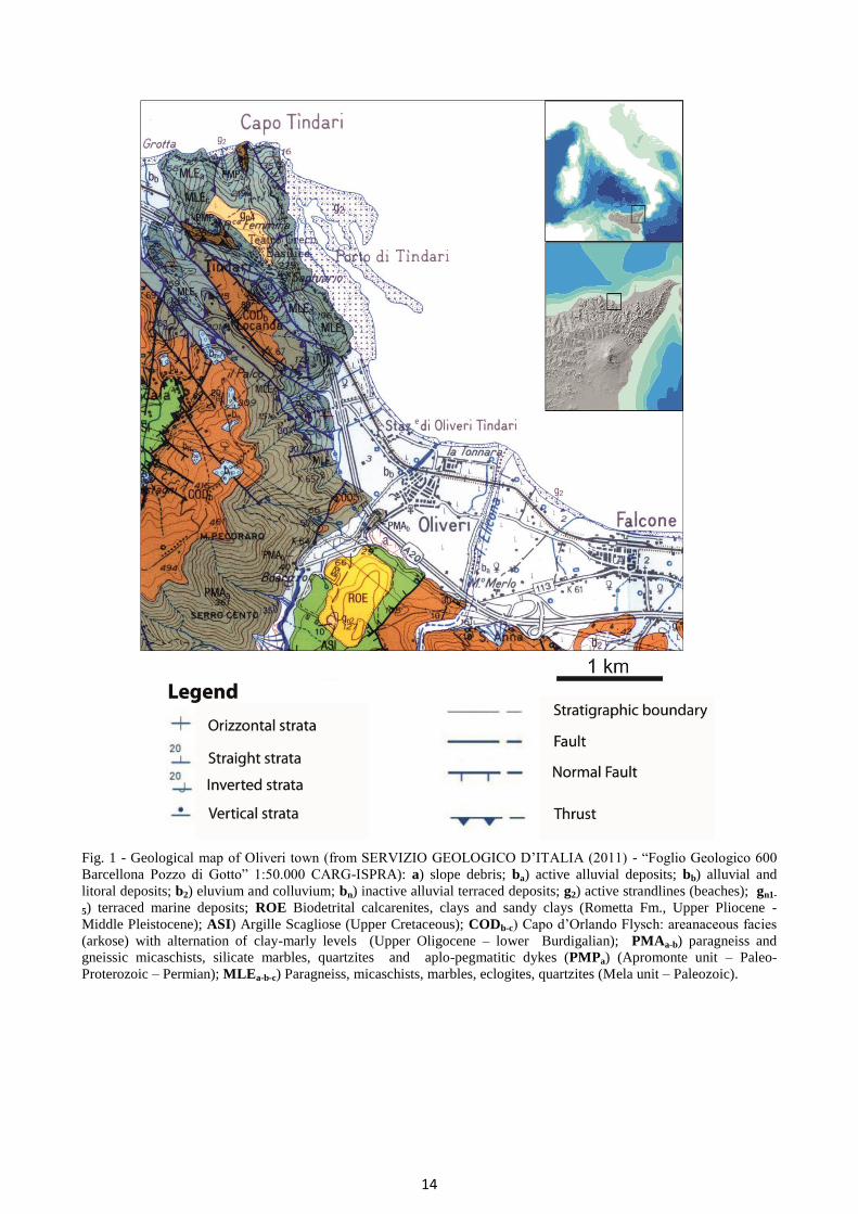
Fig. 1 - Geological map of Oliveri town (from SERVIZIO GEOLOGICO D’ITALIA (2011) - “Foglio Geologico 600

Barcellona Pozzo di Gotto” 1:50.000 CARG-ISPRA): a) slope debris; ba) active alluvial deposits; bb) alluvial and

litoral deposits; b2) eluvium and colluvium; bn) inactive alluvial terraced deposits; g2) active strandlines (beaches); gn1-

5) terraced marine deposits; ROE Biodetrital calcarenites, clays and sandy clays (Rometta Fm., Upper Pliocene -

Middle Pleistocene); ASI) Argille Scagliose (Upper Cretaceous); CODb-c) Capo d’Orlando Flysch: areanaceous facies

(arkose) with alternation of clay-marly levels (Upper Oligocene – lower Burdigalian); PMAa-b) paragneiss and

gneissic micaschists, silicate marbles, quartzites and aplo-pegmatitic dykes (PMPa) (Apromonte unit – Paleo-

Proterozoic – Permian); MLEa-b-c) Paragneiss, micaschists, marbles, eclogites, quartzites (Mela unit – Paleozoic).

15

Fig. 2 - Distribution of epicenters of instrumental earthquakes located by the INGV between 1981 and 2011.

16

Fig. 3 – HVSR analysis of the microtremor record nr. 7.

17

Fig. 4 – HVSR average curves of the clusters in which have been considered to be dominant the structural effects of 23

measures in the area of Oliveri.

18

Fig. 5 – Dendrogram of the clustering process.

19

Fig. 6 – Scatter plot of amplitude versus peak period for the four HVSR clusters and spatial distributions of three major

ones.

20

Fig. 7 – HVSR peak frequency maps of cluster B G (left) and cluster R (right). The coordinate system is WGS84

UTM.

21

Fig. 8 – Stratigraphic column of the borehole close to Torrente Elicona.

22

Fig. 9 – Inversion of the HVSR ellipticity curve of the measurement point n.7. Only the models and theoretical H/V

curves with misfit values less than 1.09 are plotted.

23

Fig. 10 – Oliveri. Left) Map of the thickness of the sedimentary cover. Right) Map of the altitude of the seismic bedrock

above sea level. The coordinate system is WGS84 UTM.

24

Fig. 11 – Oliveri. Sections representing the seismic bedrock and the soft cover. The tracks of the sections are plotted in

fig 10.