Intelligent Measurement Processes in 3D Optical Metrology: Producing More Accurate Point Clouds 

Charles Mony, Ph.D.1 President Creaform inc. cmony@creaform3D.com

Daniel Brown, Eng.1 Product Manager Creaform inc. dbrown@creaform3D.com

Patrick Hébert, Ph.D.1 3D Optical Metrology Advanced Research Creaform inc. patrick.hebert@creaform3D.com

1Creaform – 5825, rue St-Georges Lévis (Québec) Canada G6V 4L2

Word Count: 4488 Number of Images Submitted: 6

Abstract

This paper introduces the new paradigm of intelligent measurement process in the context of 3D optical metrology. Since new 3D sensor technologies can capture 3D points at very high rates on the surface of objects, it is now possible to quickly capture very dense sets of points on an object’s surface. This very large quantity of 3D point observations allows one to examine the local distribution of these points on section areas before validating their consistency with the expected error model developed at the calibration stage. From these dense point observations, higher quality surface point measurements can be produced for metrology. An intelligent measurement process will integrate these steps in real time during capture. We describe a framework adapted for implementing such a process. The result section presents some application cases in metrology. The paper concludes with prospective comments on intelligent measurement systems.

1. Introduction

It is interesting to note that scientific and technological advances have always been tightly coupled with the improvement of measuring systems. The 21st century has already witnessed the explosion of the ability to measure in several domains. Probably the most significant examples are the experiments with the CERN’s Large Hadron Collider, each generating several terabytes of observation data. Closer to our domain, existing 3D optical sensing technologies allow quick generation of a tremendous amount of dense points on the surface of an object. Indeed, capturing 20 000 to more than a million 3D points per second is no longer exotic. This ever growing capability to collect observations combined with the improved computational technologies not only paves the way to, but leads us inevitably towards the new paradigm of intelligent measurement.

Intelligent measurement is the process that produces consistent measurement obtained from a set of basic observations, and which consistency is verified against a model of the measuring process (the acquisition model) during capture. Reading an ambient temperature of 60 C in a conference room from a thermometer, or reading a diameter of 100 mm for a coin with a caliper, obviously makes no sense. One would at least make one or several additional readings before providing a reliable measurement or reporting a problem with the device. Indeed, the observation is not consistent with the expected range of values in the current context of measurement. Several

observations (readings) would be necessary to be able to confirm the consistency of each observation. Consistency is verified with respect to the acquisition model which integrates knowledge on the measuring device and hypotheses on the object to be measured. These knowledge and hypotheses may be as simple as the typical range of values and the resolution, repeatability and accuracy of the measurement that can be produced by the device. When observations are consistent, improved measurements can also be produced after reducing error due to noise, from several observations. Let’s now consider that the acquisition model is integrated within the measurement process; that would yield an intelligent measuring system. In the preceding examples, the human is the intelligent agent in the measurement process. Preferably, intelligence would be integrated into the computerized system when the quantity of observations increases and becomes intractable for the human. Integration of intelligence then becomes particularly valuable with the enormous amount of observations that can be acquired in real time with 3D optical sensors.

In this paper, it is shown how to build an intelligent measurement process in 3D optical metrology. After explaining why optical sensing technologies are well suited for the new paradigm in section 2, we will revisit the whole paradigm of raw 3D points in section 3. Actually, in any measuring system, 3D point coordinates are the results of several calculations on the observations. Moreover, their noise error distribution is not strictly identical. Section 4 develops on the principles for developing an intelligent measuring system. In section 5, we present the bases of a framework developed for implementing an intelligent measurement process. Section 6 shows various results following the application of the framework. Finally section 7 discusses the prospective in this new paradigm.

2. Capturing a large number of 3D points with optical sensors

In metrology, it is common practice to inspect parts by extracting measured characteristics from geometric entities such as spheres or planes, for instance. The characteristics are based on a limited number of calculated points from touch probe or high density cloud of points from an optical 3D sensor. It is also more and more common to evaluate the geometric conformity after comparing a 3D point cloud with a reference CAD model. During this inspection, statistics are computed on the distance between 3D points and their putative matching points that are the closest on the aligned surface model. Besides measuring points at higher density on the surface, optical sensors make it possible to avoid compensation for the radius of a tactile probe during alignment. Due to the higher point density, it is also possible to capture a dense set of points that are very close to the boundaries and crease edges.

One must keep in mind that the primary objective while inspecting a part is not to measure 3D points, but the conformity with geometric dimension and tolerance model (GD&T) in order to respect functional specifications and assembly of the product using surface geometric characteristics. Typically, 3D points measurement is a preliminary step because it is a simple and flexible way to extract surface characteristics and compare two surfaces. For instance, one may consider measuring the distance or the angle between two planes. It is clear that 3D points considered solely are of no utility since they cannot be compared. It is the underlying surface shape that is of interest. Measuring a large number of points makes it possible to better define the surfaces and entities for measuring characteristics but, furthermore, a better sampling will also allow one to characterize the error locally.

The very large number of observations that is possible with a 3D optical sensor allows the application of the new intelligent measurement paradigm described below.

3. Revisiting the paradigm of raw 3D points

In metrology, it is common practice to measure characteristics or to compare a 3D point cloud arising from a sensor to the reference surface. These observations are considered raw points, which errors are independent and identically distributed. Unfortunately, raw points do not exist, and it is erroneous to consider these measurements as raw observations. They are rather the result of several calculation steps.

For instance, in the case of a CMM-mounted touch probe, basic observations are collected from the linear or angular encoders of the system. A 3D point is then calculated from the parameters of the mechanical model of the device and the probe. These parameters are calibrated beforehand. Any error in these parameters will affect several 3D points differently and will not be independent from the measured geometry (e.g.: starting from a simple radius correction of the probe).

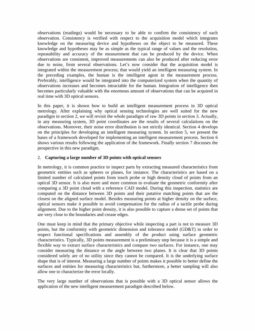
A similar situation arises with optical sensors. Let’s consider the case of a triangulation laser-based profilometer composed of a camera and a laser projector. The camera captures light and produces a 2D pixel image of the laser trace. Figure 1 illustrates a typical image section captured on an object. From this image, subpixel positions of the laser trace will be extracted. This image processing calculation involves a set of neighboring pixel values. Once these 2D positions are calculated, the system’s calibration parameters are exploited to calculate the set of 3D points. These calculations will involve image distortion correction and projection of a ray in space from the camera’s intrinsic parameters. Then, the extrinsic parameters describing the spatial relationship between the camera and the laser projector will also intervene in the computation before producing a 3D point. It is thus worth mentioning that 3D points output from sensors are the result of several computations. Their distributions are strictly neither identical nor independent. One example is shown in Figure 1, center and right.

Figure 1. Image section of a laser trace. From this image, 2D subpixel positions of the laser trace will be extracted before computing 3D points based on triangulation. Center) Cross-section captured on a corner object. Right) Distribution of the 3D points along the cross-section. The inset shows how the distribution of the 3D points differs near the corner.

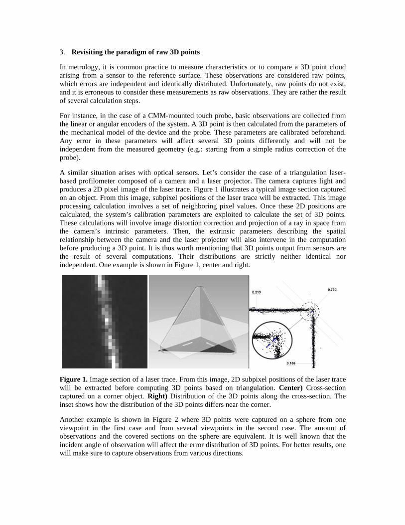
Another example is shown in Figure 2 where 3D points were captured on a sphere from one viewpoint in the first case and from several viewpoints in the second case. The amount of observations and the covered sections on the sphere are equivalent. It is well known that the incident angle of observation will affect the error distribution of 3D points. For better results, one will make sure to capture observations from various directions.

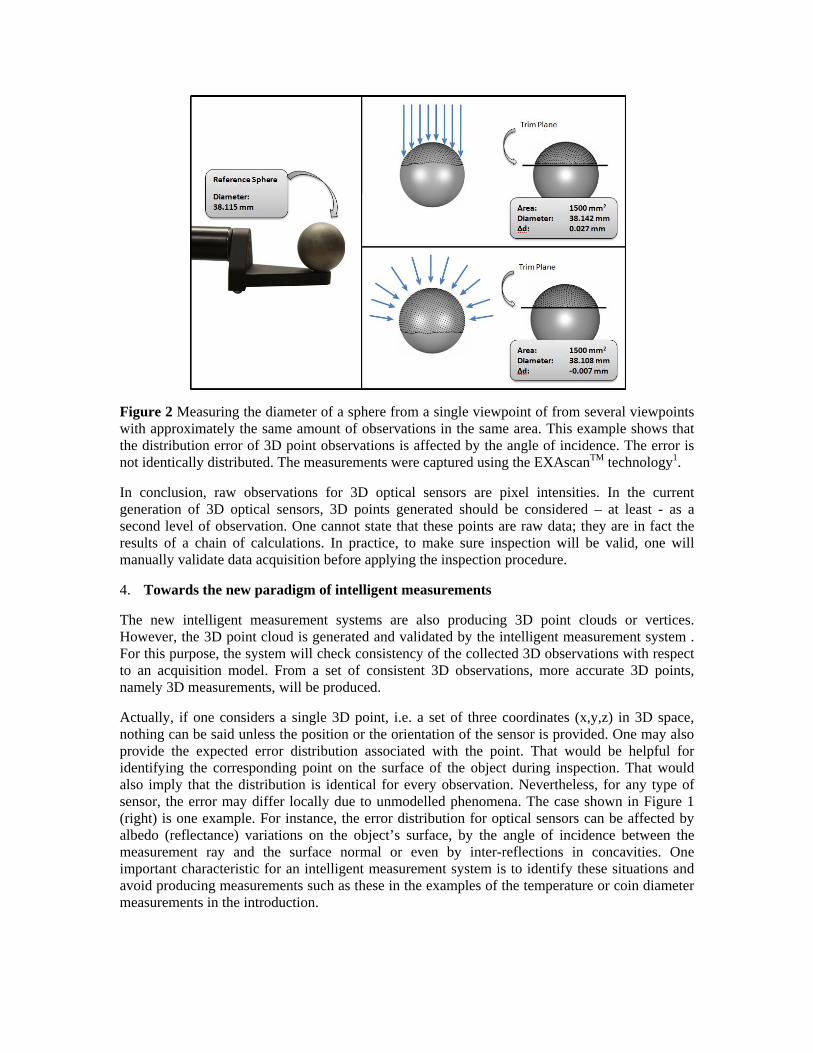
Figure 2 Measuring the diameter of a sphere from a single viewpoint of from several viewpoints with approximately the same amount of observations in the same area. This example shows that the distribution error of 3D point observations is affected by the angle of incidence. The error is not identically distributed. The measurements were captured using the EXAscanTM technology1.

In conclusion, raw observations for 3D optical sensors are pixel intensities. In the current generation of 3D optical sensors, 3D points generated should be considered – at least - as a second level of observation. One cannot state that these points are raw data; they are in fact the results of a chain of calculations. In practice, to make sure inspection will be valid, one will manually validate data acquisition before applying the inspection procedure.

4. Towards the new paradigm of intelligent measurements

The new intelligent measurement systems are also producing 3D point clouds or vertices. However, the 3D point cloud is generated and validated by the intelligent measurement system . For this purpose, the system will check consistency of the collected 3D observations with respect to an acquisition model. From a set of consistent 3D observations, more accurate 3D points, namely 3D measurements, will be produced.

Actually, if one considers a single 3D point, i.e. a set of three coordinates (x,y,z) in 3D space, nothing can be said unless the position or the orientation of the sensor is provided. One may also provide the expected error distribution associated with the point. That would be helpful for identifying the corresponding point on the surface of the object during inspection. That would also imply that the distribution is identical for every observation. Nevertheless, for any type of sensor, the error may differ locally due to unmodelled phenomena. The case shown in Figure 1 (right) is one example. For instance, the error distribution for optical sensors can be affected by albedo (reflectance) variations on the object’s surface, by the angle of incidence between the measurement ray and the surface normal or even by inter-reflections in concavities. One important characteristic for an intelligent measurement system is to identify these situations and avoid producing measurements such as these in the examples of the temperature or coin diameter measurements in the introduction.

To reach this goal, the system must gather several observations, model the local distribution of these observations and provide, from these observations, a set of measurements where the distribution is consistent with the acquisition model. This requires collecting redundant observations and testing the consistency after a sufficient number of observations are gathered. Final measurements will be calculated from these observations. Besides testing the number of accumulated observations on a surface section, the system can also monitor the variety of viewpoints from which observations have captured. The high measurement rate of optical sensors is well-suited for this task. In order to maximize the benefit of monitoring the observations, it needs to be done in real time simultaneously to the acquisition, instead of during the post-processing of the resulting point cloud.

4.1 Building an acquisition and calibration model

The acquisition model defines the expected observation in a given application context. For instance, while observing a planar opaque surface in the direction normal to the surface, at a given distance, the average and covariance matrix of 3D observations (x,y,z) can be modeled beforehand, either empirically or analytically. This refers to the repeatability of the measurement. One will also evaluate the accuracy of the system using an independent reference for comparison. Although the performances of a system can be assessed independently, the characterization is also performed during calibration with a reference object. Of course, the acquisition model can be more sophisticated while considering a wider spectrum of acquisition conditions or, conversely, modeling very specific conditions for a dedicated application (e.g. measuring the skin surface geometry of a human body).

Following the case of a triangulation-based optical sensor, the procedure encompasses the geometric calibration of the camera and optics as well as the calibration of the laser projector. In the first case, a photogrammetric camera model may be used. The intrinsic (internal) parameters include the principal point, pixel scale and eventually skew as well as distortion typically modeled with radial and tangential parameters. One must also calibrate the extrinsic (external) parameters of the structure assembly with the camera and the laser projector. These parameters are necessary for applying 3D triangulation. Since the laser projector might not be perfect, its distortion must also be modeled. An alternative to the explicit calibration parameters would be building an implicit model in the form of lookup tables. In this case, the sensor is moved precisely relatively to a calibration target, and the positions of the laser trace in the image are extracted and registered at each incremental step. These are classical approaches and the quality of the measurement will depend on the quality of hardware components, the calibration target as well as the processing algorithms.

One can go one step further with the intelligent measurement system. Actually, one can apply different calibration models depending on the environment. For instance, it is possible to adapt the acquisition model based on the distance between the sensor and the surface of the object or based on environmental measurements such as temperature that will affect the physical arrangement of the sensor. This provides the sensor with basic intelligence since it adapts to the conditions. One can still go further and characterize the influence of the measured geometry on the noise level by considering the surface angle of incidence or the local curvature. This reaches a higher level of intelligence since the system must capture observations and estimate the environmental conditions including the observed shape before refining the parameters of the acquisition model. In the end, measurements of better quality can be obtained with a given set of hardware components.

5. Data structure and surface representation for intelligent measurements

In addition to providing an acquisition model, a system capable of intelligent measurements should be suited for accumulating an unlimited quantity of 3D observations along with their associated sensor pose. It should also permit local assessment of the consistency of these accumulated 3D observations with respect to the acquisition model before producing 3D measurements. These requirements impose a data structure for managing all the 3D information. Since the 3D observations are captured on the surface of an object, it is expected that the data structure will encode a representation of the observed surface. While explicit surfaces such as triangulated meshes are the most commonly used surface representations for 3D modeling and computer graphics, they are ill-adapted for efficiently managing the accumulation of 3D observations in a continuous process. For these reasons, volumetric representations of implicit surfaces have been developed in the last 15 years2,3,4.

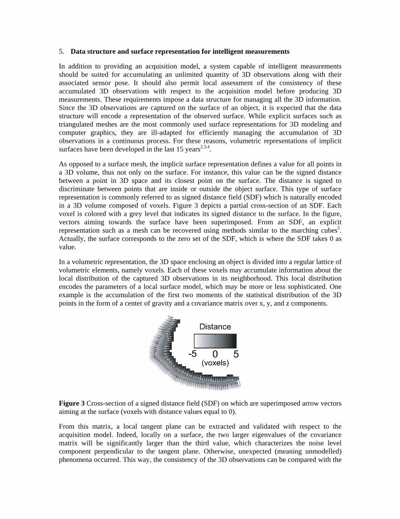
As opposed to a surface mesh, the implicit surface representation defines a value for all points in a 3D volume, thus not only on the surface. For instance, this value can be the signed distance between a point in 3D space and its closest point on the surface. The distance is signed to discriminate between points that are inside or outside the object surface. This type of surface representation is commonly referred to as signed distance field (SDF) which is naturally encoded in a 3D volume composed of voxels. Figure 3 depicts a partial cross-section of an SDF. Each voxel is colored with a grey level that indicates its signed distance to the surface. In the figure, vectors aiming towards the surface have been superimposed. From an SDF, an explicit representation such as a mesh can be recovered using methods similar to the marching cubes5. Actually, the surface corresponds to the zero set of the SDF, which is where the SDF takes 0 as value.

In a volumetric representation, the 3D space enclosing an object is divided into a regular lattice of volumetric elements, namely voxels. Each of these voxels may accumulate information about the local distribution of the captured 3D observations in its neighborhood. This local distribution encodes the parameters of a local surface model, which may be more or less sophisticated. One example is the accumulation of the first two moments of the statistical distribution of the 3D points in the form of a center of gravity and a covariance matrix over x, y, and z components.

Figure 3 Cross-section of a signed distance field (SDF) on which are superimposed arrow vectors aiming at the surface (voxels with distance values equal to 0).

From this matrix, a local tangent plane can be extracted and validated with respect to the acquisition model. Indeed, locally on a surface, the two larger eigenvalues of the covariance matrix will be significantly larger than the third value, which characterizes the noise level component perpendicular to the tangent plane. Otherwise, unexpected (meaning unmodelled) phenomena occurred. This way, the consistency of the 3D observations can be compared with the

expected noise level from the sensor 3D observations and thus be validated. For instance, in Figure 1, the system can invalidate data close to the intersection of the two planes where inter-reflections affect the distribution of observations. In the same way, the number of observed points and the distribution of sensor positions where the 3D points have been collected are accumulated at each voxel for further validation. From such a volumetric representation, there is no limit on the quantity of observations that can be captured and processed.

The online application of this paradigm was unconceivable only 10 years ago due to the required computer resources including memory and computation. Today, it can be applied on commodity hardware. In order to reduce computational costs, the field is computed only in the neighborhood of the surface, i.e. at points that are closer to the surface than a predetermined constant distance T > 0 where T will depend on the sensor’s noise characteristic. This neighborhood is said to be enclosed by a volumetric envelope. Being defined as the zero-crossing of the norm (which occurs between neighboring voxels), the surface is adequately represented as long as T is larger than the voxel's diagonal (the largest distance between two neighboring voxels).

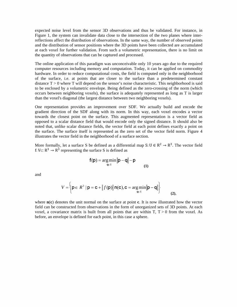
One representation provides an improvement over SDF. We actually build and encode the gradient direction of the SDF along with its norm. In this way, each voxel encodes a vector towards the closest point on the surface. This augmented representation is a vector field as opposed to a scalar distance field that would encode only the signed distance. It should also be noted that, unlike scalar distance fields, the vector field at each point defines exactly a point on the surface. The surface itself is represented as the zero set of the vector field norm. Figure 4 illustrates the vector field in the neighborhood of a surface section.

More formally, let a surface S be defined as a differential map S: U R R . The vector field f: V R R representing the surface S is defined as

pqppfq

Sminarg)(

(1)

and

qpccn pcpp

q SfRV minarg),()(|3

(2),

where n(c) denotes the unit normal on the surface at point c. It is now illustrated how the vector field can be constructed from observations in the form of unorganized sets of 3D points. At each voxel, a covariance matrix is built from all points that are within T, T > 0 from the voxel. As before, an envelope is defined for each point, in this case a sphere.

Figure 4 Example of the vector field. a) The vector field is computed on a regular grid of points (voxel centers) so that the vector at each voxel center points towards the closest surface point. The field is defined only in the vicinity of the surface, which is in the volumetric envelope (region bounded by two iso-distant surfaces, coloured in green). b) A cross-section of the vector field.

The covariance matrix is obtained as follows:

N

i

TTii

Ti

N

ii NN

C11

1))((

1 cccc (3)

where

N

iiN 1

1 c (4),

is the centroid of closest points ci. Both and matrix C can be computed incrementally. The normal is obtained as the eigenvector associated with the smallest eigenvalue. The distribution of the sensor orientation is also easily cumulated in the voxels.

Finally, those voxels that accumulated a significant number of consistent observations in their neighborhood contribute to producing a set of output 3D point measurements. The consistency test described beforehand is based on the eigenvalues of the covariance matrix. It can be further validated using the distribution of sensor directions. The output measurements are obtained after applying a modified version of the marching cubes algorithm that is actually adapted to vector fields.

6. Application

Based on this data and surface representation, acquisition model and calibration, a first generation of intelligent measuring systems with 3D optical sensors were implemented. These intelligent measuring systems introduce the new paradigm presented in this article to the market place for concrete applications. One major and immediate result of this new intelligent measuring system that can be easily demonstrated is that increasing the number of observations (multiple acquisition) increases the accuracy of the measurement instead of creating noise in the point cloud.

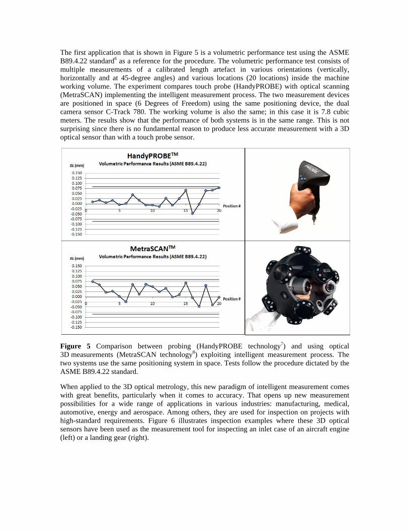
The first application that is shown in Figure 5 is a volumetric performance test using the ASME B89.4.22 standard6 as a reference for the procedure. The volumetric performance test consists of multiple measurements of a calibrated length artefact in various orientations (vertically, horizontally and at 45-degree angles) and various locations (20 locations) inside the machine working volume. The experiment compares touch probe (HandyPROBE) with optical scanning (MetraSCAN) implementing the intelligent measurement process. The two measurement devices are positioned in space (6 Degrees of Freedom) using the same positioning device, the dual camera sensor C-Track 780. The working volume is also the same; in this case it is 7.8 cubic meters. The results show that the performance of both systems is in the same range. This is not surprising since there is no fundamental reason to produce less accurate measurement with a 3D optical sensor than with a touch probe sensor.

Figure 5 Comparison between probing (HandyPROBE technology7) and using optical 3D measurements (MetraSCAN technology8) exploiting intelligent measurement process. The two systems use the same positioning system in space. Tests follow the procedure dictated by the ASME B89.4.22 standard.

When applied to the 3D optical metrology, this new paradigm of intelligent measurement comes with great benefits, particularly when it comes to accuracy. That opens up new measurement possibilities for a wide range of applications in various industries: manufacturing, medical, automotive, energy and aerospace. Among others, they are used for inspection on projects with high-standard requirements. Figure 6 illustrates inspection examples where these 3D optical sensors have been used as the measurement tool for inspecting an inlet case of an aircraft engine (left) or a landing gear (right).

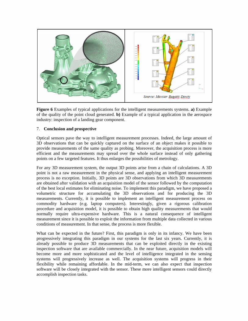
Figure 6 Examples of typical applications for the intelligent measurements systems. a) Example of the quality of the point cloud generated. b) Example of a typical application in the aerospace industry: inspection of a landing gear component.

7. Conclusion and prospective

Optical sensors pave the way to intelligent measurement processes. Indeed, the large amount of 3D observations that can be quickly captured on the surface of an object makes it possible to provide measurements of the same quality as probing. Moreover, the acquisition process is more efficient and the measurements may spread over the whole surface instead of only gathering points on a few targeted features. It thus enlarges the possibilities of metrology.

For any 3D measurement system, the output 3D points arise from a chain of calculations. A 3D point is not a raw measurement in the physical sense, and applying an intelligent measurement process is no exception. Initially, 3D points are 3D observations from which 3D measurements are obtained after validation with an acquisition model of the sensor followed by the computation of the best local estimates for eliminating noise. To implement this paradigm, we have proposed a volumetric structure for accumulating the 3D observations and for producing the 3D measurements. Currently, it is possible to implement an intelligent measurement process on commodity hardware (e.g. laptop computers). Interestingly, given a rigorous calibration procedure and acquisition model, it is possible to obtain high quality measurements that would normally require ultra-expensive hardware. This is a natural consequence of intelligent measurement since it is possible to exploit the information from multiple data collected in various conditions of measurement. In that sense, the process is more flexible.

What can be expected in the future? First, this paradigm is only in its infancy. We have been progressively integrating this paradigm in our systems for the last six years. Currently, it is already possible to produce 3D measurements that can be exploited directly in the existing inspection software that are available commercially. In the near future, acquisition models will become more and more sophisticated and the level of intelligence integrated in the sensing systems will progressively increase as well. The acquisition systems will progress in their flexibility while remaining affordable. In the mid-term, we can also expect that inspection software will be closely integrated with the sensor. These more intelligent sensors could directly accomplish inspection tasks.

References

1. EXAscan technology, http://www.creaform3D.com/en/handyscan3D/products/exascan.aspx, site consulted on May 13, 2011.

2. Hilton, Adrian and Illingworth, John, Geometric fusion for a hand-held 3D sensor. Machine vision and applications, 12:44–51, 2000.

3. Curless, Brian and Levoy, Marc, A volumetric method for building complex models from range images, In SIGGRAPH ’96 Conference Proceedings, pages 303–312, August 1996.

4. Masuda, Takeshi, Registration and Integration of Multiple Range Images by Matching Signed Distance Fields for Object Shape Modeling, Computer Vision and Image Understanding, 87:51–65, January 2003.

5. Lorensen, William and Cline, Harvey. Marching cubes: A high resolution 3D surface construction algorithm. SIGGRAPH ’87 Conference Proceedings, 21(4):163–169, 1987.

6. The American Society of Mechanical Engineers, American National Standard ASME B89.4.22- 2004, Method for Performance Evaluation of Articulated Arm Coordinate Measuring Machine, 2005.

7. HandyPROBE technology, http://www.creaform3D.com/en/handyprobe/handyprobe.aspx, site consulted on May 13, 2011.

8. MetraSCAN technology, http://www.creaform3D.com/en/metrascan/default.aspx, site consulted on May 13, 2011.