Intelligent Tutoring Systems Using Reinforcement

Learning

A THESIS

submitted by

SREENIVASA SARMA B. H.

for the award of the degree

of

MASTER OF SCIENCE(by Research)

DEPARTMENT OF COMPUTER SCIENCE AND ENGINEERINGINDIAN INSTITUTE OF TECHNOLOGY, MADRAS.

MAY 2007

THESIS CERTIFICATE

This is to certify that the thesis entitled Intelligent Tutoring Systems using Rein-forcement Learning submitted by Sreenivasa Sarma .B. H. to the Indian Institute of

Technology, Madras for the award of the degree of Master of Science (by Research)

is a bona-fide record of research work carried out by him under my supervision. The

contents of this thesis, in full or in parts, have not been submitted to any other Institute

or University for the award of any degree or diploma.

Chennai - 600036 Dr. B. Ravindran

Date: Dept. of Computer Science and Engg.

ACKNOWLEDGEMENTS

I am immensely grateful to Dr. B. Ravindran for his guidance and encouragement dur-

ing my research work. His relentless pursuit of excellence, his unconventional approach

to research and his inexhaustible levels of energy have been a source of inspiration to

me. I am thankful to him for the patience he has shown in me.

I thank Prof. Timothy A. Gonsalves for providing excellent facilities in the depart-

ment for research. I am highly indebted to him for his kind consideration and help,

towards the continuation of my research work.

I thank the members of the General Test Committee, Prof. S. Srinivasan and

Prof. V. Kamakoti for their interest in my research work and their valuable comments

and suggestions on my work. I particularly thank Prof. B. Yegnanarayana, former Gen-

eral Test Committee member, for his encouragement and suggestions in initial stage of

my research work.

I thank Dr. N. Sudha, former adviser, for her support during early days of my re-

search work.

I am thankful to all the faculty and non-teaching staff within the department as well

as outside the department for all the help that I have received during my stay at IIT

Madras.

I thank my senior laboratory members Surya, Krishnamohan, Kumaraswamy, Dha-

nunjaya (Dhanu), Guru, Anil, and Murthy for all the cooperation, understanding and

help I have received from them.

I thank other members of the lab, Anand, Swapna, Ved, Harindra, Harnath, Dilip,

and Veena for their cooperation during my work at the lab.

I specially thank Laxmi Narayana Panuku (Lax), Sheetal (Dada), Krishna Prasad

(Kothi), Prashant (Prash), Rakesh Bangani (Rocky), Lalit, Siddartha (Sidhu), Ramakr-

i

ishna (Rama), Bhanu, Seenu (PETA), Mani (Manee), Anil kumar (Saddam), Abhilash

(Abhi), and Noor (Peddanna) for the good times. I have thoroughly enjoyed their com-

pany.

I thank Rammohan for his great help during my struggle at IIT Madras, which

helped me to continue my research work.

I would like to thank all my teachers, relatives and friends whose blessings and

wishes have helped me reach this far.

Words can not express the profoundness of my gratitude to my parents

Smt. B. H. Meenakshi and Shri. B. H. Janardhana Rao, whose love and blessings are a

constant source of strength to me.

I thank my brother Mallikarjuna Sarma (Malli) for his cooperation and help in dif-

ferent stages of my life.

ii

ABSTRACT

Intelligent Tutoring System (ITS) is an interactive and effective way of teaching stu-

dents. ITS gives instructions about a topic to a student, who is using it. The student has

to learn the topic from an ITS by solving problems. The system gives a problem and

compares the solution it has with that of the student’s and then it evaluates the student

based on the differences. The system continuously updates a student model by interact-

ing with the student. Usually, ITS uses artificial intelligence techniques to customize its

instructions according to the student’s need. For this purpose the system should have

the knowledge of the student (student model) and the set of pedagogical rules. Disad-

vantages of these methods are, it is hard to encode all pedagogical rules, it is difficult

to incorporate the knowledge that human teachers use and it is difficult to maintain a

student model and also these systems are not adaptive to new student’s behavior.

To overcome these disadvantages we use Reinforcement Learning (RL) to take

teaching actions. RL learns to teach, given only the state description of the student

and reward. Here, the student model is just the state description of the student, which

reduces the cost and time of designing ITS. The RL agent uses the state description as

the input to a function approximator, and uses the output of the function approximator

and reward, to take a teaching action. To validate and to improve the ITS we have ex-

perimented with teaching a simulated student using the ITS. We have considered issues

in teaching a special case of students suffering from autism. Autism is a disorder of

communication, socialization and imagination. An Artificial Neural Network (ANN)

with backpropagation is selected as simulated student, that shares formal qualitative

similarities with the selective attention and generalization deficits seen in people with

autism. Our experiments show that an autistic student can be taught as effectively as a

normal student using the proposed ITS.

iii

TABLE OF CONTENTS

ACKNOWLEDGEMENTS i

ABSTRACT iii

LIST OF FIGURES ix

ABBREVIATIONS x

IMPORTANT NOTATION xi

1 Introduction 1

1.1 Components of an ITS . . . . . . . . . . . . . . . . . . . . . . . . 2

1.1.1 Student model . . . . . . . . . . . . . . . . . . . . . . . . 2

1.1.2 Pedagogical module . . . . . . . . . . . . . . . . . . . . . 3

1.1.3 Domain module . . . . . . . . . . . . . . . . . . . . . . . . 3

1.2 Reinforcement learning . . . . . . . . . . . . . . . . . . . . . . . . 3

1.3 Simulated student . . . . . . . . . . . . . . . . . . . . . . . . . . . 4

1.4 Issues in designing ITS . . . . . . . . . . . . . . . . . . . . . . . . 4

1.4.1 Domain module representation . . . . . . . . . . . . . . . . 5

1.4.2 Student model . . . . . . . . . . . . . . . . . . . . . . . . 5

1.4.3 Pedagogical module . . . . . . . . . . . . . . . . . . . . . 5

1.5 Structure of the thesis . . . . . . . . . . . . . . . . . . . . . . . . . 6

2 Existing ITSs - A Review 7

2.1 Early ITSs . . . . . . . . . . . . . . . . . . . . . . . . . . . . . . . 7

2.2 Recent developments in ITSs . . . . . . . . . . . . . . . . . . . . . 8

2.2.1 Student models . . . . . . . . . . . . . . . . . . . . . . . . 9

2.2.2 Pedagogical modules . . . . . . . . . . . . . . . . . . . . . 9

2.2.3 AnimalWatch . . . . . . . . . . . . . . . . . . . . . . . . . 10

iv

2.2.4 ADVISOR . . . . . . . . . . . . . . . . . . . . . . . . . . 10

2.2.5 Wayang Outpost . . . . . . . . . . . . . . . . . . . . . . . 11

2.2.6 AgentX . . . . . . . . . . . . . . . . . . . . . . . . . . . . 11

2.3 Other ITSs . . . . . . . . . . . . . . . . . . . . . . . . . . . . . . . 11

3 Mathematical Background 13

3.1 Terms used in reinforcement learning . . . . . . . . . . . . . . . . 13

3.1.1 Markov decision process . . . . . . . . . . . . . . . . . . . 13

3.1.2 State-values and Action-values . . . . . . . . . . . . . . . . 14

3.1.3 Temporal Difference learning . . . . . . . . . . . . . . . . 15

3.1.4 Function approximation . . . . . . . . . . . . . . . . . . . 17

3.2 Artificial neural networks . . . . . . . . . . . . . . . . . . . . . . . 18

3.2.1 Artificial neural networks for pattern classification tasks . . 19

3.2.2 Multi-layer Artificial neural networks with backpropogation 22

4 Design of RL based ITS 25

4.1 Motivation for using Reinforcement Learning . . . . . . . . . . . . 25

4.2 Proposed model of ITS using RL . . . . . . . . . . . . . . . . . . . 26

4.3 RL algorithm designed for the pedagogical module . . . . . . . . . 28

4.4 Issues . . . . . . . . . . . . . . . . . . . . . . . . . . . . . . . . . 30

4.4.1 Reward function . . . . . . . . . . . . . . . . . . . . . . . 30

4.4.2 State representation . . . . . . . . . . . . . . . . . . . . . . 30

4.4.3 Action set . . . . . . . . . . . . . . . . . . . . . . . . . . . 31

4.5 Artificial neural networks as simulated student . . . . . . . . . . . . 31

4.5.1 Autism and its effects . . . . . . . . . . . . . . . . . . . . . 32

5 Evaluation of the proposed ITS 34

5.1 Classification Problem . . . . . . . . . . . . . . . . . . . . . . . . 34

5.1.1 Artificial neural network architecture . . . . . . . . . . . . 35

5.2 Problem #1 : Four classes . . . . . . . . . . . . . . . . . . . . . . . 35

5.2.1 Experiments . . . . . . . . . . . . . . . . . . . . . . . . . 37

5.2.2 Results . . . . . . . . . . . . . . . . . . . . . . . . . . . . 38

v

5.3 Problem #2 : Three classes . . . . . . . . . . . . . . . . . . . . . . 48

5.3.1 Experiments . . . . . . . . . . . . . . . . . . . . . . . . . 48

5.3.2 Results . . . . . . . . . . . . . . . . . . . . . . . . . . . . 49

5.4 Problem #3 : Five classes . . . . . . . . . . . . . . . . . . . . . . . 55

5.4.1 Experiments and Results . . . . . . . . . . . . . . . . . . . 55

5.5 Experiments with different learning rates for different classes . . . . 56

5.6 Issues addressed . . . . . . . . . . . . . . . . . . . . . . . . . . . . 60

5.6.1 Reward function . . . . . . . . . . . . . . . . . . . . . . . 60

5.6.2 State representation . . . . . . . . . . . . . . . . . . . . . . 62

5.6.3 Domain module . . . . . . . . . . . . . . . . . . . . . . . . 62

6 Mapping the proposed ITS into the Real-World Situation 64

6.1 Real-world situation . . . . . . . . . . . . . . . . . . . . . . . . . . 64

6.1.1 Domain module . . . . . . . . . . . . . . . . . . . . . . . . 64

6.1.2 Student model . . . . . . . . . . . . . . . . . . . . . . . . 65

6.1.3 User-system interface . . . . . . . . . . . . . . . . . . . . . 66

6.2 Mapping . . . . . . . . . . . . . . . . . . . . . . . . . . . . . . . . 67

6.2.1 Domain module . . . . . . . . . . . . . . . . . . . . . . . . 67

6.2.2 Student model or state representation . . . . . . . . . . . . 67

7 Conclusion and Future work 68

7.1 Summary of the contribution: . . . . . . . . . . . . . . . . . . . . 69

7.2 Other Applications . . . . . . . . . . . . . . . . . . . . . . . . . . 69

LIST OF FIGURES

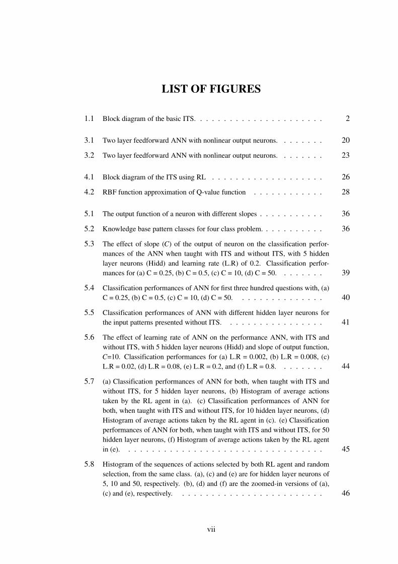
1.1 Block diagram of the basic ITS. . . . . . . . . . . . . . . . . . . . . . 2

3.1 Two layer feedforward ANN with nonlinear output neurons. . . . . . . . 20

3.2 Two layer feedforward ANN with nonlinear output neurons. . . . . . . . 23

4.1 Block diagram of the ITS using RL . . . . . . . . . . . . . . . . . . . 26

4.2 RBF function approximation of Q-value function . . . . . . . . . . . . 28

5.1 The output function of a neuron with different slopes . . . . . . . . . . . 36

5.2 Knowledge base pattern classes for four class problem. . . . . . . . . . . 36

5.3 The effect of slope (C) of the output of neuron on the classification perfor-mances of the ANN when taught with ITS and without ITS, with 5 hiddenlayer neurons (Hidd) and learning rate (L.R) of 0.2. Classification perfor-mances for (a) C = 0.25, (b) C = 0.5, (c) C = 10, (d) C = 50. . . . . . . . 39

5.4 Classification performances of ANN for first three hundred questions with, (a)C = 0.25, (b) C = 0.5, (c) C = 10, (d) C = 50. . . . . . . . . . . . . . . 40

5.5 Classification performances of ANN with different hidden layer neurons forthe input patterns presented without ITS. . . . . . . . . . . . . . . . . 41

5.6 The effect of learning rate of ANN on the performance ANN, with ITS andwithout ITS, with 5 hidden layer neurons (Hidd) and slope of output function,C=10. Classification performances for (a) L.R = 0.002, (b) L.R = 0.008, (c)L.R = 0.02, (d) L.R = 0.08, (e) L.R = 0.2, and (f) L.R = 0.8. . . . . . . . 44

5.7 (a) Classification performances of ANN for both, when taught with ITS andwithout ITS, for 5 hidden layer neurons, (b) Histogram of average actionstaken by the RL agent in (a). (c) Classification performances of ANN forboth, when taught with ITS and without ITS, for 10 hidden layer neurons, (d)Histogram of average actions taken by the RL agent in (c). (e) Classificationperformances of ANN for both, when taught with ITS and without ITS, for 50hidden layer neurons, (f) Histogram of average actions taken by the RL agentin (e). . . . . . . . . . . . . . . . . . . . . . . . . . . . . . . . . . 45

5.8 Histogram of the sequences of actions selected by both RL agent and randomselection, from the same class. (a), (c) and (e) are for hidden layer neurons of5, 10 and 50, respectively. (b), (d) and (f) are the zoomed-in versions of (a),(c) and (e), respectively. . . . . . . . . . . . . . . . . . . . . . . . . 46

vii

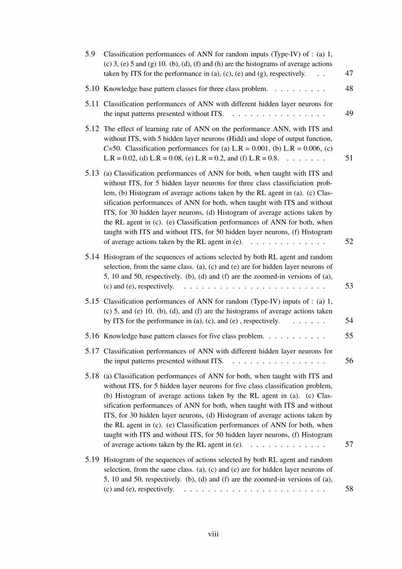
5.9 Classification performances of ANN for random inputs (Type-IV) of : (a) 1,(c) 3, (e) 5 and (g) 10. (b), (d), (f) and (h) are the histograms of average actionstaken by ITS for the performance in (a), (c), (e) and (g), respectively. . . 47

5.10 Knowledge base pattern classes for three class problem. . . . . . . . . . 48

5.11 Classification performances of ANN with different hidden layer neurons forthe input patterns presented without ITS. . . . . . . . . . . . . . . . . 49

5.12 The effect of learning rate of ANN on the performance ANN, with ITS andwithout ITS, with 5 hidden layer neurons (Hidd) and slope of output function,C=50. Classification performances for (a) L.R = 0.001, (b) L.R = 0.006, (c)L.R = 0.02, (d) L.R = 0.08, (e) L.R = 0.2, and (f) L.R = 0.8. . . . . . . . 51

5.13 (a) Classification performances of ANN for both, when taught with ITS andwithout ITS, for 5 hidden layer neurons for three class classificiation prob-lem, (b) Histogram of average actions taken by the RL agent in (a). (c) Clas-sification performances of ANN for both, when taught with ITS and withoutITS, for 30 hidden layer neurons, (d) Histogram of average actions taken bythe RL agent in (c). (e) Classification performances of ANN for both, whentaught with ITS and without ITS, for 50 hidden layer neurons, (f) Histogramof average actions taken by the RL agent in (e). . . . . . . . . . . . . . 52

5.14 Histogram of the sequences of actions selected by both RL agent and randomselection, from the same class. (a), (c) and (e) are for hidden layer neurons of5, 10 and 50, respectively. (b), (d) and (f) are the zoomed-in versions of (a),(c) and (e), respectively. . . . . . . . . . . . . . . . . . . . . . . . . 53

5.15 Classification performances of ANN for random (Type-IV) inputs of : (a) 1,(c) 5, and (e) 10. (b), (d), and (f) are the histograms of average actions takenby ITS for the performance in (a), (c), and (e) , respectively. . . . . . . 54

5.16 Knowledge base pattern classes for five class problem. . . . . . . . . . . 55

5.17 Classification performances of ANN with different hidden layer neurons forthe input patterns presented without ITS. . . . . . . . . . . . . . . . . 56

5.18 (a) Classification performances of ANN for both, when taught with ITS andwithout ITS, for 5 hidden layer neurons for five class classification problem,(b) Histogram of average actions taken by the RL agent in (a). (c) Clas-sification performances of ANN for both, when taught with ITS and withoutITS, for 30 hidden layer neurons, (d) Histogram of average actions taken bythe RL agent in (c). (e) Classification performances of ANN for both, whentaught with ITS and without ITS, for 50 hidden layer neurons, (f) Histogramof average actions taken by the RL agent in (e). . . . . . . . . . . . . . 57

5.19 Histogram of the sequences of actions selected by both RL agent and randomselection, from the same class. (a), (c) and (e) are for hidden layer neurons of5, 10 and 50, respectively. (b), (d) and (f) are the zoomed-in versions of (a),(c) and (e), respectively. . . . . . . . . . . . . . . . . . . . . . . . . 58

viii

5.20 (a), (c) and (e) are classification performances of the ANN (Type-I), for four-class classification problem, with different learning rates for different classes.The learning rates are (a) 0.2, 0.4, 0.6 and 0.8 for classes A, B, C and D,respectively. (c) 0.6, 0.4, 0.2 and 0.3 and (e) 0.8, 0.6, 0.4 and 0.2. (b), (d)and (f) are the histograms of average actions taken by ITS for (a), (c) and (e)respectively. . . . . . . . . . . . . . . . . . . . . . . . . . . . . . . 59

5.21 (a), (c) and (e) are classification performances of the ANN (Type-I), for three-class classification problem, with different learning rates for different classes.The learning rates are (a) 0.2, 0.4, and 0.6 for classes A, B, and C, respectively.(b) 0.6, 0.4, and 0.2 and (c) 0.6, 0.8 and 0.2. (b), (d) and (f) are the histogramsof average actions taken by ITS for (a), (c) and (e) respectively. . . . . . 61

6.1 Prototype of a Mathematics tutor . . . . . . . . . . . . . . . . . . . . 65

6.2 Prototype of a Mathematics tutor providing hint to a question on area of arectangle . . . . . . . . . . . . . . . . . . . . . . . . . . . . . . . . 66

ix

ABBREVIATIONS

CAI Computer Aided Instructions

CBT Computer Based Training

ITS Intelligent Tutoring Systems

RL Reinforcement Learning

ANN Artificial Neural Networks

PSM Population Student Model

PA Pedagogical Agent

BN Bayesian Network

BNN Biological Neural Networks

MDP Markov Decision process

TD-learning Temporal Difference Learning

RBF Radial Basis Function

x

IMPORTANT NOTATION

rt Reward to the RL agent at time, t

γ Discount factor of the expected future reward of the RL agent

ε Factor of the exploration in state space of the RL agent

α Position of RBFs in the state space

ρ Width of each RBF

β,βh Learning rates of the RL agent

π(s,a) Policy followed by the RL agent at state, s and action a

Q(s,a) Expected total future reward or Q-value of the RL agent for state, s and action a

Qπ(.) Action-value function for policy, π

Rt Total future reward at time, t, in an RL agent

A(s) Action space for state, s

Eπ. Expectation give that π is followed

El Mean square error between desired and obtained outputs of the ANN for l th input pattern

et Error between expected future reward and the obtained reward

η Learning rate of the ANN

C Slope of the output function of ANN

xi

CHAPTER 1

Introduction

People have been interested in using computers for education for a long time. Intelli-

gent tutors have many benefits for education. Students can learn different subjects if the

intelligent tutors are designed to adapt to the curriculum. The student can learn by him-

self through this type of learning, which is similar to one-to-one tutoring. One-to-one

teaching by human tutors has been shown to increase the average student’s performance

to around ninety-eight percent of students in a normal classroom [1, 2]. It also has been

shown in [3] that intelligent tutors can produce the same improvement that results from

one-to-one human tutoring and can effectively reduce by one-third to one-half the time

required for learning.

Computer aided instruction (CAI) and Computer-based training (CBT) were the

first systems developed to teach using computers. In these type of systems, instructions

were not customized to the learners needs. Instead, the decisions about how to move a

student through the material were rule-based, such as “if question 21 is answered cor-

rectly, present question 54 to the student; otherwise present question 32”. The learner’s

abilities were not taken into account [4]. But these do not provide the same kind of

individualized attention that a student would receive from a human tutor. To provide

such attention Intelligent Tutoring Systems (ITS) have been developed.

One of the important goals of this thesis is to design an ITS which adapts itself to

students with different learning abilities. The other goal is to reduce the knowledge

engineering work needed to develop an ITS. ITSs obtains their teaching decisions by

representing pedagogical rules about how to teach and information about the student.

A student learns from an ITS by solving problems. The system selects a problem

and compares its solution with that of the student’s and then it evaluates the student

based on the differences. After giving feedback, the system re-evaluates and updates

the student model and the entire cycle is repeated. As the system is learning what

the student knows, it also considers what the student needs to know, which part of the

curriculum is to be taught next, and how to present the material. It then selects the

problems accordingly. Section 1.1 describes basic ITS with different components in it.

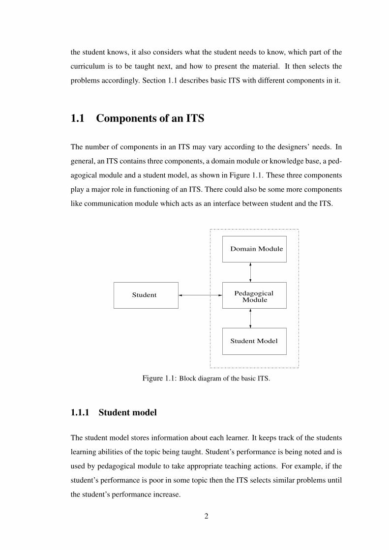
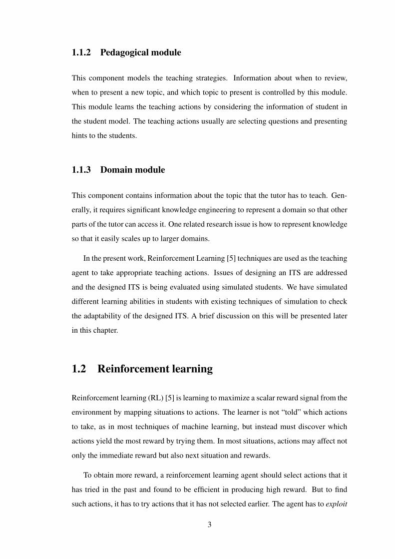
1.1 Components of an ITS

The number of components in an ITS may vary according to the designers’ needs. In

general, an ITS contains three components, a domain module or knowledge base, a ped-

agogical module and a student model, as shown in Figure 1.1. These three components

play a major role in functioning of an ITS. There could also be some more components

like communication module which acts as an interface between student and the ITS.

Domain Module

Student Module

Pedagogical

Student Model

Figure 1.1: Block diagram of the basic ITS.

1.1.1 Student model

The student model stores information about each learner. It keeps track of the students

learning abilities of the topic being taught. Student’s performance is being noted and is

used by pedagogical module to take appropriate teaching actions. For example, if the

student’s performance is poor in some topic then the ITS selects similar problems until

the student’s performance increase.

2

1.1.2 Pedagogical module

This component models the teaching strategies. Information about when to review,

when to present a new topic, and which topic to present is controlled by this module.

This module learns the teaching actions by considering the information of student in

the student model. The teaching actions usually are selecting questions and presenting

hints to the students.

1.1.3 Domain module

This component contains information about the topic that the tutor has to teach. Gen-

erally, it requires significant knowledge engineering to represent a domain so that other

parts of the tutor can access it. One related research issue is how to represent knowledge

so that it easily scales up to larger domains.

In the present work, Reinforcement Learning [5] techniques are used as the teaching

agent to take appropriate teaching actions. Issues of designing an ITS are addressed

and the designed ITS is being evaluated using simulated students. We have simulated

different learning abilities in students with existing techniques of simulation to check

the adaptability of the designed ITS. A brief discussion on this will be presented later

in this chapter.

1.2 Reinforcement learning

Reinforcement learning (RL) [5] is learning to maximize a scalar reward signal from the

environment by mapping situations to actions. The learner is not “told” which actions

to take, as in most techniques of machine learning, but instead must discover which

actions yield the most reward by trying them. In most situations, actions may affect not

only the immediate reward but also next situation and rewards.

To obtain more reward, a reinforcement learning agent should select actions that it

has tried in the past and found to be efficient in producing high reward. But to find

such actions, it has to try actions that it has not selected earlier. The agent has to exploit

3

what it already knows, to obtain high reward, but it has to explore to make better action

selection in future. One of the challenges that arise in reinforcement learning is the

trade-off between exploration and exploitation. To know more about reinforcement

learning, the basic terms and concepts of RL, refer section 3.1 of this thesis.

1.3 Simulated student

The advancement in technology has made it possible for computers to “learn” skills and

knowledge in different fields. All types of machine learning techniques have shown sig-

nificant development, especially within the last couple of decades [6]. Empirical work

on human learning of higher level skills and knowledge has also expanded significantly

during this period. Using simulated students, teachers can develop and practice their

teaching skills on simulated students and instruction designers can test their products,

in order to get precise feedback early in the design process. In this thesis, we have used

simulated students for evaluating our proposed ITS due to these advantages.

One of the possibilities of simulating the students’ learning behavior is through

Artificial Neural Networks (ANN). A detailed description of ANNs is in section 3.2

and its application as simulated student is dealt in section 4.5.

1.4 Issues in designing ITS

While designing an ITS, the designer has to consider numerous issues, including do-

main module representation, student representation and pedagogical decisions, to im-

prove the performance and usability of the ITS. Apart from those discussed below there

are some other issues related to user-interface design, etc.,The following are some of

such essential issues that should be contemplated while designing an ITS:

4

1.4.1 Domain module representation

Domain module representation is one of the important issues to be considered while

designing an ITS. In general, this module comprises of the questions and hints on a

topic to be taught to the student. These questions and hints should be represented such

that the pedagogical module could interact effectively with this module and could select

appropriate questions and hints that are needed by the student while learning. If the

representation is not compatible with the pedagogical module then the tutoring system

would under-perform.

1.4.2 Student model

Student model plays a key role in representing the students’ knowledge on a topic. In an

ideal case, the student model should be exact replica of the students’ knowledge. There

are some machine learning sophisticated techniques to model the students’ proficiency.

For example, Bayesian networks, ANN and rule-based models form good models of

the human students’ learning [6]. While updating the student model the ITS should

keep contemplating the students’ performance for all past questions asked. If the ITS

estimates the students’ knowledge inaccurately then there is a possibility of misleading

students by presenting irrelevant questions and through unnecessary hint or suggestions.

1.4.3 Pedagogical module

The pedagogical module contains the teaching strategies. While interacting with the

student model, the pedagogical module decides which question to be selected further

for the student so that he/she could master the topic it is being taught. The pedagogical

module should be designed such that the appropriate teaching action is taken at appro-

priate time. For this purpose machine learning techniques such as Bayesian networks

and rule-based methods are being used, which are explained in-detail in section 2.2. But

as mentioned earlier, in the present work reinforcement learning techniques are applied

as a pedagogical module. We will empirically verify in later chapters of the thesis that

this would improve the teaching performance of the tutoring system and also makes the

5

system adaptive to the students’ learning abilities.

1.5 Structure of the thesis

The existing work on ITSs is covered briefly in chapter 2. A brief mathematical back-

ground, for the further understanding of the thesis, is presented in chapter 3. Chap-

ter 4 describes processes involved in the proposed ITS. In section 4.4, issues that arise

while using reinforcement learning are discussed in detail. While chapter 5 presents the

performance of the proposed ITS with experiments and results. As the proposed ITS

is being evaluated using simulated students, a brief description of the mapping of this

work into real-world situation i.e., to teach human students, is given in chapter 6. Chap-

ter 7 concludes this thesis with some suggestions that would help to further improve this

ITS.

6

CHAPTER 2

Existing ITSs - A Review

The range of tasks that an Intelligent Tutoring System has to perform is vast ranging

from primary and simple to extremely complicated. For example, the interface to the

student can range from a command line interface or a graphical user interface to an

interface that can perform natural language processing. The tutoring systems can be

implemented in various ways ranging from simple man-machine dialog to an intelligent

companion, where the computer can learn the material along with the student. In this

chapter, we will explore some of the prominent ITSs that have been developed so far.

2.1 Early ITSs

Initially, people who were interested in student models concentrated on procedural “er-

rors” made by a population of students in a particular domain that could be explicitly

represented in the student model. The term “bug” was used to indicate “procedural

mistakes”, i.e., the correct execution of an incorrect procedure, rather then fundamental

misconceptions. The study of “bugs” resulted in development of an ITS, BUGGY – “a

descriptive theory of bugs whereby the model enumerates observable bugs”.

BUGGY was developed in 1975 by J. S. Brown and R. R. Burton. Initially, it was

developed after the study of protocols produced by students that related to algebraic

operation such as the subtraction of multi digit numbers. The early studies of students

doing algebra, revealed the need for a special representation, which could represent

each skill which they do not learn independently. This allowed the design of a model

which would reflect the students’ understanding of the skills and sub skills involved in

a task.

The knowledge representation model for this study was the procedural network,

which was an attempt to break down the larger task into a number of related subtasks.

The modeling methods involved substituting buggy variants of individual sub skills into

the procedural network in an attempt to reproduce the behavior of the student.

Rather than providing BUGGY with the tutorial skills needed to recognize and

counter act student mistakes, the developers of BUGGY focused on developing a com-

plete model of the student that can give information for their evaluation. They attempted

to count the different possible procedural bugs students might acquire while trying to

solve math problems.

Reverse to the usual roles of ITS, teacher and student, BUGGY used its student

model to simulate a student with “buggy” thinking. The educator then diagnosed the

student bug based on BUGGY’s examples. Using its table of possible bugs, BUGGY

could generate general tests to identify students’ mistakes, such as “the student subtracts

the smaller digit in each column from the larger digit regardless of which is on top”.

Later Burton developed a DEBUGGY system which uses a perturbation construct to

represent a student’s knowledge as variants of the fine grain procedural structure of the

correct skill.

Many of the early ITSs tried to produce a model of the student from his observable

behavior [7]. Algorithms for producing such models dealt with the issues of “credit”

allotment, combinational explosion when producing mixed concepts out of primitives,

and removing noisy data. The assignment-of-credit problem deals with determining

how to intelligently allocate blame i.e., crediting for having caused a failure, when

more than one primary step is necessary of success. This problem is, when there is

failure on a task that requires multiple skills, which skill does not the student have. An

analogous problem is allocating credit for success among methods when there is more

than one successful method.

2.2 Recent developments in ITSs

In recent past, there was lot of work done in modeling students knowledge using ma-

chine learning techniques [8, 9, 10]. CLAR-ISSE [10] is an ITS that uses machine

learning to initialize the student model by the method of classifying the students into

8

learning groups. ANDES [11] is a Newtonian physics tutor that uses a Bayes Nets ap-

proach to create a student model to decide what type of help to make available to the

student by keeping track of the students progress within a specific physics problem,

their knowledge of physics and their goals for solving a problem.

2.2.1 Student models

In [12], authors have modeled the students learning through Bayesian networks. They

used Expectation Maximization technique to find the model parameters that maximize

the expected value of the log-likelihood, where the data for the expected values are

replaced by using their expected value for the observed students’ knowledge. They used

clustering models of the students, like grouping different students into different learning

groups for updating their learning behavior, i.e., the student model. The authors in [13]

used dynamic Bayesian networks (DBN) to model the students learning behavior over

a time period. They have considered two states, either mastered or not mastered, for

each problem system asked and the observables are also two, either correct or incorrect.

They also considered hints to evaluated student, i.e, the DBN also learns the students

performance when both the hint is presented and not presented.

SAFARI [14] updates the student model using curriculum-based knowledge repre-

sentation. The student model in this case is a complex structure with three components,

the Cognitive Model, the Interference Model and the Affective Model. Some of the

elements of the student model depends on the course, like some pedagogical resources,

but others elements such as capabilities of students cam be general and can be reused to

another context.

2.2.2 Pedagogical modules

As opposed to the earlier systems, where only the representation of student was con-

sidered, in present day ITSs intelligence in taking pedagogical actions is also consid-

ered, which lead to the drastic improvement in the performance of the tutoring systems.

Case-Based Reasoning (CBR) was used as the pedagogical modules to teach students

9

in some cases such as [15, 16, 17]. Authors in [17] used CBR to teach learner using

hypermedia educational services which are similar to ITSs, but through Internet. They

have developed an Adaptive Hypermedia System (AHS) which adapts to the learner.

But the disadvantage of these systems is its extensive knowledge engineering work. For

taking a pedagogical decision, lot of cases need to be checked and coding/developing

such case becomes complicated with the context. There are some other ITSs which uses

different machine learning techniques like reinforcement learning and BNN for taking

pedagogical decisions. Brief discussions on such ITSs are in the following sections.

2.2.3 AnimalWatch

AnimalWatch [18] was an intelligent tutor that teaches arithmetic to grade school stu-

dents. The goal of the tutor was to improve girls’ self-confidence in their ability to

do mathematics. It was a mathematics tutor that used machine learning to the prob-

lem of generating new problems, hints and help. AnimalWatch learned how to predict

some characteristics of student problem solving such as number of mistakes made or

time spent on each problem. It used this model to automatically compute an optimal

teaching policy, such as reducing mistakes made or time spent on each problem.

2.2.4 ADVISOR

The ADVISOR [19] was developed to reduce the amount of knowledge engineering

needed to construct an ITS and to make the tutor’s teaching goals parameterized so

that they can be altered as per the need. For this purpose, machine learning techniques

were used. In an ADVISOR, there are two machine learning agents. One of them is a

Population Student Model (PSM), which has the data about the students who used Ani-

malWatch. PSM is responsible for predicting how student will perform in this situation.

The second agent is pedagogical agent (PA), which is given the PSM as input. The PA’s

task is to experiment with the PSM to find a teaching policy that will meet the provided

teaching goal.

The pedagogical agent is a reinforcement learning agent, that can operate with the

10

model of the environment (the PSM) and a reward function. The disadvantage of the

ADVISOR is its PSM, which is not generalized and also it is not accurate in predicting

the correctness of the student response.

2.2.5 Wayang Outpost

Wayang Outpost [20] is a web-based tutoring system designed to teach mathematics

for students appearing for SAT examination. The most effective part of this tutoring

system is its user-interface, which uses sound and animation to teach students. Problem

are presented to the student and if the student answers incorrectly or asks for hints, the

teacher character provides step-by-step instruction and guidance in the form of Flash

animation and audio. This tutor also used to investigate the interaction of gender and

cognitive skills in mathematics problem solving, and in selecting pedagogical approach.

The student model is a Bayesian Network (BN) which is trained with the data obtained

from the students who used the tutoring system off-line. It divides the student knowl-

edge based on the skill set he acquired. The nodes of the BN represent the skills of the

student on particular topic.

2.2.6 AgentX

AgentX [21] also uses RL to learn teaching actions, it groups the students using it into

different levels and then selects questions or hints for the student according to the level

he/she is in. The students’ level will be changing according to his present knowledge

status. Grouping students into different levels and then instructing is an abstract way of

teaching a student. There is possibility of generalizing the students which may not be

the effective way of teaching.

2.3 Other ITSs

Tutoring systems are not only used for teaching curriculum based subjects like mathe-

matics, physics etc., but also for teaching medical and military skills [22]. For example,

11

the Cardiac Tutor helped students learn an established medical procedure through di-

rected practice within an intelligent simulation [23]. It contains required domain knowl-

edge about cardiac resuscitation and was designed for training medical personnel in the

skills of advanced cardiac life support (ACLS) [24]. The system evaluated student

performance according to procedures established by the American Heart Association

(AHA) and provided extensive feedback to the students. There are some tutors devel-

oped for teaching military commands and skills [25]. For example, ComMentor is being

developed to teach complicated military skills [26].

In chapter 3, a brief description of reinforcement learning and artificial neural net-

works is given, making it comfortable to understand further chapters in this thesis.

12

CHAPTER 3

Mathematical Background

Reinforcement Learning (RL) [5] is learning to map situations to actions, that can in-

crease a numerical value called reward. The RL agent is not informed which actions

to take, instead it should know by itself which actions give the most reward by trying

them. To get high reward, an RL agent must select actions that it tried in the past and

found to be effective in producing high reward. But to find such actions, it has to try

actions that it has not tried already.

3.1 Terms used in reinforcement learning

An RL system contains a policy, a reward function and a value function. A policy is

the learning agent’s method of selecting actions at a given time. It is the mapping of

environment state to the appropriate action to be taken when it is in that states. A reward

function specifies the goal in an RL problem that maps each state of the environment in

which it is present to a single number, a reward. The value of a state is the total amount

of reward an agent can expect to accumulate over the future, starting from that state.

In RL framework, the agent makes its decisions as a function of a signal from the

environment’s state, s. A state signal, is that which summarizes past sensations in such

a way that all relevant information is obtained. This usually needs more or less the

complete history of all past sensations. A state signal is called Markov or has Markov

property, if it succeeds in obtaining all relevant information.

3.1.1 Markov decision process

An RL task that obeys the Markov property is called a Markov decision process or

MDP. If the state and action spaces are finite, then it is called a f inite Markov decision

process (finite MDP). Finite MDPs are particularly important to the theory of RL.

It is relevant to think of a state in RL as an approximation to a Markov state, though

the state signal is non-Markov. The state should be designed such that it should pre-

dict the subsequent states in cases where a environment model is learned. This can be

achieved by using Markov states. The RL agent gives better performance if the state is

designed to be Markov or at least is designed to approaches the Markov state. So, it is

useful to assume the state to be approximately Markov at each time step even though it

may not fully satisfy the Markov property. Theory applicable for the Markov case can

be applied to most of the tasks with states that are not fully Markov.

3.1.2 State-values and Action-values

The value function specifies the total future reward that can be expected or the expected

return at a state, which is the value of that state. The value functions are defined with

respect to particular policies. Let S be the set of possible states and A(s) be the set

of actions taken in state s, then the policy, π, is a mapping from each state, s ∈ S and

action, a ∈ A(s), to the probability π(s,a) of taking an action, a, in state, s. The value

of a state, s, following a policy π, defined as V π(s), is the expected return while starting

in s and following π from there. For MDPs, we can define V π(s) as

V π(s) = Eπ Rt |st = s

= Eπ

∞

∑k=0

γkrt+k+1|st = s

(3.1)

where Eπ represents the expected value given that the agent follows policy π, rt+k+1

is the reward for (t + k + 1)th time step and γ is the discount factor. The value of the

terminal state will be always zero. The function V π is called the state-value function

for policy, π. Similarly, the value of taking action a in state s under a policy π, denoted

Qπ(s,a), as the expected return starting from s, taking the action a, and from there

following policy π:

Qπ(s,a) = Eπ Rt |st = s,at = a

= Eπ

∞

∑k=0

γkrt+k+1|st = s,at = a

(3.2)

14

where Qπ is called the action-value function for policy, π.

The RL agent has to find a policy that gives a high reward in long run which is

called an optimal policy. An optimal policy is defined as the policy π that is better than

or equal to a policy π′ if its expected return is greater than or equal to that of π′ for all

states, in a finite MDP. Always there will be an optimal policy in a task. All the optimal

policies are represented by π∗, and their value functions are denoted by V ∗ and Q∗.

3.1.3 Temporal Difference learning

Temporal Difference (TD) learning methods can be used to estimate these value func-

tions. If the value functions were to be calculated without estimation then the agent

would need to wait until the final reward was received before any state-action pair val-

ues could be updated. Once the final reward was received, the path taken to reach the

final state would need to be traced back and each value updated accordingly. This could

be expressed as:

V (st)←V (st)+α[Rt−V (st)] (3.3)

(or)

Q(st,a)←Q(st ,a)+α[Rt−Q(st ,a)] (3.4)

where st is the state visited at time t,a and Rt are the action taken and the reward

after time t respectively, and α is a constant parameter.

Instead, with TD method, an estimate of the final reward is calculated at every state

and the state-action value updated for every step. There are two ways of TD-learning

i.e., On-Policy and Off-Policy.

On-Policy and Off-Policy Learning

On-Policy Temporal Difference methods learn the value of the policy that is used to

make decisions. The value functions are updated using results from executing actions

by following some policy. These policies are usually “soft” and non-deterministic. The

15

meaning of “soft” in this case is that it makes clear, there is always an element of

exploration to the policy. The policy is not confined to always choosing the action that

gives the most reward. Three common policies are used, ε-soft, ε-greedy and softmax.

Off-Policy methods can learn different policies for behavior and estimation. The

behavior policy is usually “soft” so there is sufficient exploration going on. Off-policy

algorithms can update the estimated value functions using actions that have not actually

been tried. This is in contrast to on-policy methods which update value functions based

strictly on experience. What this means is off-policy algorithms can separate explo-

ration from control, and on-policy algorithms cannot. In other words, an agent trained

using an off-policy method may end up learning tactics that it did not necessarily exhibit

during the learning phase.

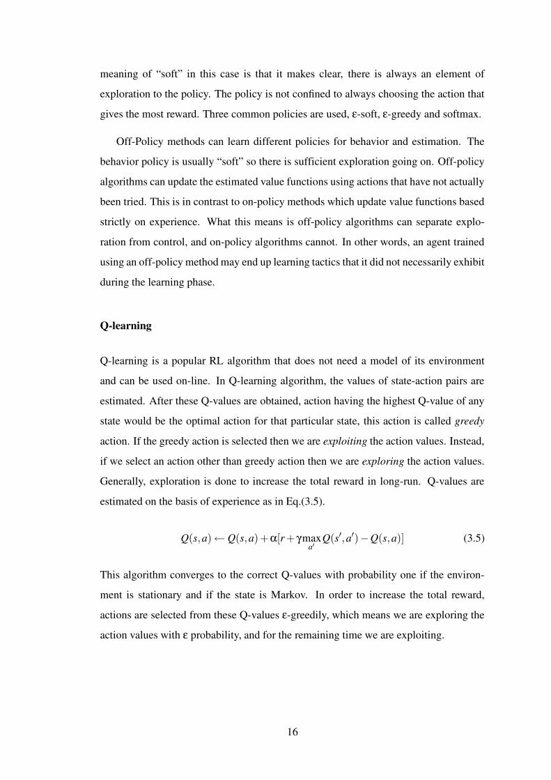
Q-learning

Q-learning is a popular RL algorithm that does not need a model of its environment

and can be used on-line. In Q-learning algorithm, the values of state-action pairs are

estimated. After these Q-values are obtained, action having the highest Q-value of any

state would be the optimal action for that particular state, this action is called greedy

action. If the greedy action is selected then we are exploiting the action values. Instead,

if we select an action other than greedy action then we are exploring the action values.

Generally, exploration is done to increase the total reward in long-run. Q-values are

estimated on the basis of experience as in Eq.(3.5).

Q(s,a)← Q(s,a)+α[r + γmaxa′

Q(s′,a′)−Q(s,a)] (3.5)

This algorithm converges to the correct Q-values with probability one if the environ-

ment is stationary and if the state is Markov. In order to increase the total reward,

actions are selected from these Q-values ε-greedily, which means we are exploring the

action values with ε probability, and for the remaining time we are exploiting.

16

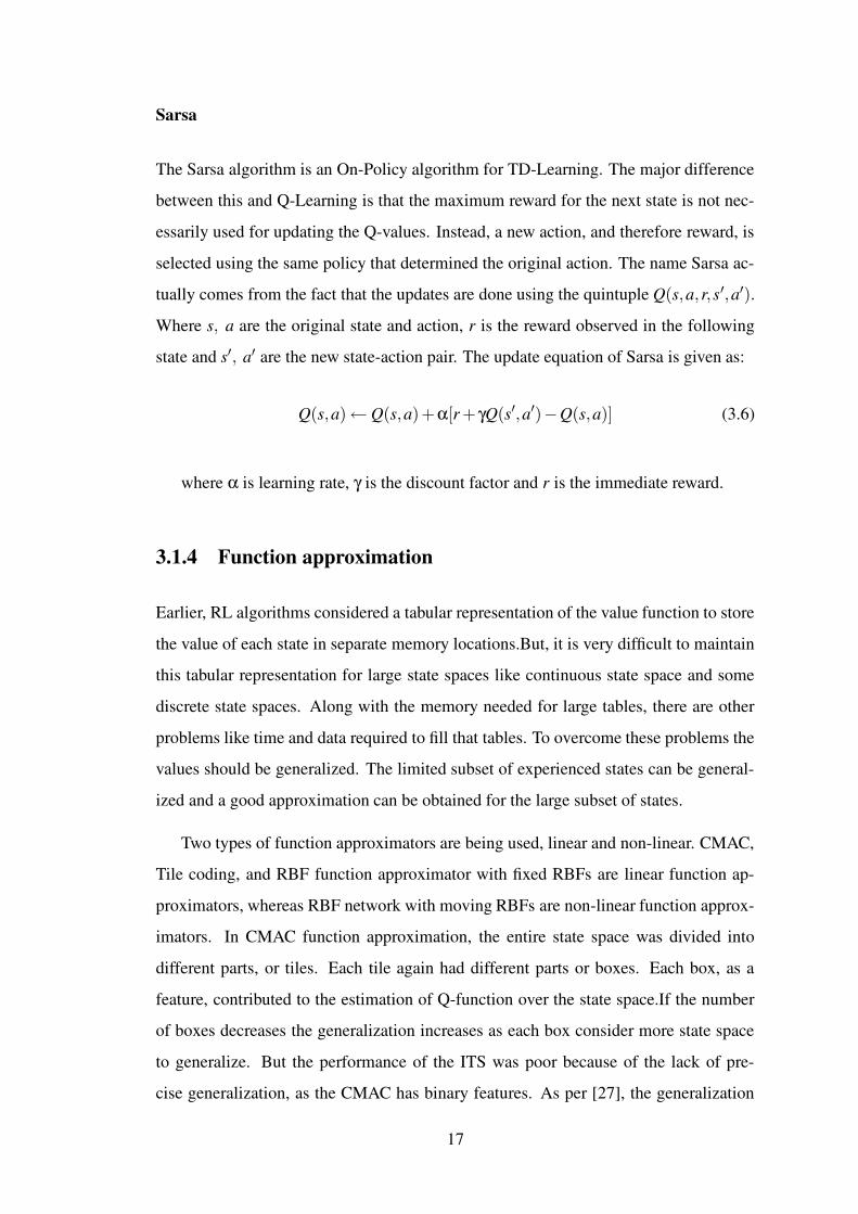
Sarsa

The Sarsa algorithm is an On-Policy algorithm for TD-Learning. The major difference

between this and Q-Learning is that the maximum reward for the next state is not nec-

essarily used for updating the Q-values. Instead, a new action, and therefore reward, is

selected using the same policy that determined the original action. The name Sarsa ac-

tually comes from the fact that the updates are done using the quintuple Q(s,a,r,s′,a′).

Where s, a are the original state and action, r is the reward observed in the following

state and s′, a′ are the new state-action pair. The update equation of Sarsa is given as:

Q(s,a)←Q(s,a)+α[r + γQ(s′,a′)−Q(s,a)] (3.6)

where α is learning rate, γ is the discount factor and r is the immediate reward.

3.1.4 Function approximation

Earlier, RL algorithms considered a tabular representation of the value function to store

the value of each state in separate memory locations.But, it is very difficult to maintain

this tabular representation for large state spaces like continuous state space and some

discrete state spaces. Along with the memory needed for large tables, there are other

problems like time and data required to fill that tables. To overcome these problems the

values should be generalized. The limited subset of experienced states can be general-

ized and a good approximation can be obtained for the large subset of states.

Two types of function approximators are being used, linear and non-linear. CMAC,

Tile coding, and RBF function approximator with fixed RBFs are linear function ap-

proximators, whereas RBF network with moving RBFs are non-linear function approx-

imators. In CMAC function approximation, the entire state space was divided into

different parts, or tiles. Each tile again had different parts or boxes. Each box, as a

feature, contributed to the estimation of Q-function over the state space.If the number

of boxes decreases the generalization increases as each box consider more state space

to generalize. But the performance of the ITS was poor because of the lack of pre-

cise generalization, as the CMAC has binary features. As per [27], the generalization

17

could be improved by having feature values continuously varying in range of [0,1], so

an RBF network is chosen for further FA in this work. The RBFs with varying widths

and centers could generalize precisely because of its nonlinearity.

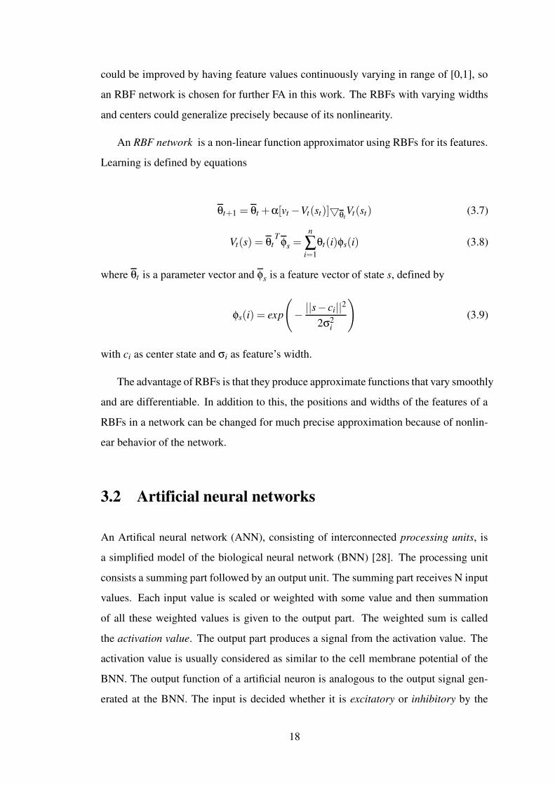
An RBF network is a non-linear function approximator using RBFs for its features.

Learning is defined by equations

θt+1 = θt +α[vt−Vt(st)]5θtVt(st) (3.7)

Vt(s) = θtT φs =

n∑i=1

θt(i)φs(i) (3.8)

where θt is a parameter vector and φs is a feature vector of state s, defined by

φs(i) = exp(

−||s− ci||2

2σ2i

)

(3.9)

with ci as center state and σi as feature’s width.

The advantage of RBFs is that they produce approximate functions that vary smoothly

and are differentiable. In addition to this, the positions and widths of the features of a

RBFs in a network can be changed for much precise approximation because of nonlin-

ear behavior of the network.

3.2 Artificial neural networks

An Artifical neural network (ANN), consisting of interconnected processing units, is

a simplified model of the biological neural network (BNN) [28]. The processing unit

consists a summing part followed by an output unit. The summing part receives N input

values. Each input value is scaled or weighted with some value and then summation

of all these weighted values is given to the output part. The weighted sum is called

the activation value. The output part produces a signal from the activation value. The

activation value is usually considered as similar to the cell membrane potential of the

BNN. The output function of a artificial neuron is analogous to the output signal gen-

erated at the BNN. The input is decided whether it is excitatory or inhibitory by the

18

sign of the weight for each input. It is excitatory for positive weights and inhibitory for

negative. The inputs and outputs can be discrete or continuous values and also can be

deterministic or stochastic.

The weights of the connecting links in a network are adjusted for a network to learn

the pattern in the given input data. All the weights of the connections at a particular

time is called the weight state, which can be viewed as a point in the weight space.

The trajectory of the weight states in the weight space are determined by the synaptic

dynamics of the network.

3.2.1 Artificial neural networks for pattern classification tasks

If a set of M-dimensional input patterns are divided into different classes, then for each

input pattern in different classes is assigned an output pattern called class label, which is

unique to each class. Generally, for pattern classification problems, the output patterns

are points in a discrete N-dimensional space.

Two layer feedforward Artificial neural network

A two layer feedforward network, as shown in Figure 3.1, with nonlinear output func-

tions for the units in the output layer can be used to perform the task of pattern clas-

sification. The number of units in the input layer is should be equal to the dimension-

ality of the input vectors. The units in the input layer are all linear, as the input layer

contributes very less to fan out the input to each of the output units. The number of out-

put units depends on the number of different classes in the pattern classification task.

Each unit in first layer is connected to all the inputs of the next layer, and a weight is

assigned to each connection. By including the second layer in the network, the con-

straint on the number of input patterns that the number of input-output pattern pairs to

be associated must be limited to the dimensionality of input patterns, can be overcome.

But the inclusion of the second layer introduces the limitation on linear separability

of functional relation between input and output patterns which leads to a harder clas-

sif ication problem (not linearly separable classes in the input). This hard problem can

be solved by using a multilayer artificial neural network, which is discussed briefly in

19

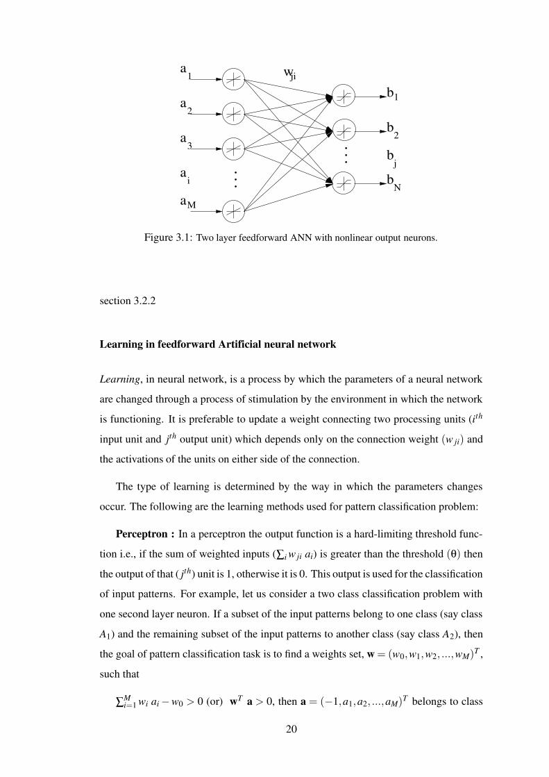
a

a

a

a1

2

3

M

b

b

b

1

2

N

w

ai

bj

ji

......

Figure 3.1: Two layer feedforward ANN with nonlinear output neurons.

section 3.2.2

Learning in feedforward Artificial neural network

Learning, in neural network, is a process by which the parameters of a neural network

are changed through a process of stimulation by the environment in which the network

is functioning. It is preferable to update a weight connecting two processing units (ith

input unit and jth output unit) which depends only on the connection weight (w ji) and

the activations of the units on either side of the connection.

The type of learning is determined by the way in which the parameters changes

occur. The following are the learning methods used for pattern classification problem:

Perceptron : In a perceptron the output function is a hard-limiting threshold func-

tion i.e., if the sum of weighted inputs (∑i w ji ai) is greater than the threshold (θ) then

the output of that ( jth) unit is 1, otherwise it is 0. This output is used for the classification

of input patterns. For example, let us consider a two class classification problem with

one second layer neuron. If a subset of the input patterns belong to one class (say class

A1) and the remaining subset of the input patterns to another class (say class A2), then

the goal of pattern classification task is to find a weights set, w = (w0,w1,w2, ...,wM)T ,

such that

∑Mi=1 wi ai−w0 > 0 (or) wT a > 0, then a = (−1,a1,a2, ...,aM)T belongs to class

20

A1. Otherwise, a belongs to class A2

Perceptron learning law: In the above perceptron classification problem, the input

space is an M−dimensional space and the number of output patterns are two, corre-

sponding to the two classes. The objective of the perceptron learning is to adjust the

weights for each presentation of an input vector belonging (called an “echo”) to A1 or

A2 along with its class identification (desired output). The perceptron learning law for

the two-class problem may be stated as

w(m+1) = w(m)+η a, i f a ∈ A1 and wT (m)a≤ 0 (3.10)

= w(m)−η a, i f a ∈ A2 and wT (m)a≥ 0 (3.11)

It has been proved [28] that the perceptron learning law converges in a finite number

of steps, provided that the given classification problem is representable.

Perceptron learning as gradient descent : The perceptron learning law in Eq.(3.10)

can also be written as

w(m+1) = w(m)+η(b(m)− s(m)) a(m) (3.12)

where b(m) is the desired output . For binary case it is given by

b(m) = 1, f or a(m) ∈ A1 (3.13)

= 0, f or a(m) ∈ A2 (3.14)

ans s(m) is the actual output for the input vector a(m) to the perceptron. The actual

output is given by

s(m) = 1, i f wT (m)a(m) > 0 (3.15)

= 0, i f wT (m)a(m)≤ 0 (3.16)

Eq. (3.12) is also valid for a bipolar output function, i.e., when s(m) = f (wT (m) a(m)) =

21

±1. So, Eq. (3.12) can be written as

w(m+1) = w(m)+η e(m) a(m) (3.17)

where e(m) = b(m)− s(m) is the error signal. If the instantaneous correlation (prod-

uct) of the output error e(m) and the activation value x(m) = wT (m) a(m) is used as a

measure of performance E(m), then

E(m) =−e(m)x(m) =−e(m)wT (m)a(m) (3.18)

The negative derivative of E(m) with respect to the weight vector w(m) can be defined

as the negative gradient of E(m) and is given by

−∂E(m)

∂w(m)= e(m) a(m) (3.19)

Thus the weight update η e(m) a(m) in the perceptron learning in Eq. (3.17) is propor-

tional to the negative gradient of the performance measure E(m).

3.2.2 Multi-layer Artificial neural networks with backpropogation

A two-layer feedforward network with hard-limiting threshold units in the output layer

can solve linearly separable pattern classification problems. There are many problems

which are not linearly separable, and are not representable by a single layer perceptron.

These problems which are not representable are called hard problems. By adding more

layers (multilayer as shown in Figure (3.2 ) ) with nonlinear units to a network can solve

the pattern classification problem of nonlinearly separable pattern classes.

A gradient descent approach is followed to reduce the error between the desired and

actual output. A generalized delta rule or backpropogation is the learning algorithm in

which the gradient is back propagated to the previous layers to adjust the weights such

that the error at the output is minimized. Following is the backpropogation algorithm

for a two-layered ANN :

Given a set of input-output patterns (al,bl), l = 1,2, ...,L where the lth input vector

22

... ...

...

a1

a

a

a

2

i

I

b

b

b

b

1

2

K

k

w wji kj

1

2

I

1

2

K

J

3

2

1

Figure 3.2: Two layer feedforward ANN with nonlinear output neurons.

is al = (al1,al2, ...,alI)T and the lth output vector is bl = (bl1,bl2, ...,blK)T . Let the

initial weights (w ji and wk j, f or1≤ i≤ I,1≤ j≤ Jand1≤ k ≤ K) be arbitrary and the

input layer has linear units. Then the output signal is equal to the input activation value

for each of these units.

Let η be the learning rate parameter. Let a = a(m) = al and b = b(m) = bl .

Activation of the unit i in the input layer, xi = ai(m)

Activation of unit j in the hidden layer, x j = ∑Ii=1 w jixi

Output signal from the jth unit in the hidden layer, s j = f ′j(x j), where f ′(.) is the

output function of the hidden layer neurons.

Activation of the unit k in the output layer, xk = ∑Jj=1 wk js j

Output signal from the unit k in the output layer , sk = fk(xk), where f (.) is the

output function of the output layer neurons.

Error term for the kth output unit, δk = (bk− sk) fk, where f (.) is the differentiation

of function f (.).

Now the weights of the output layer are updated using this error as

wk j(m+1) = wk j(m)+η δk s j (3.20)

23

Error term for the jth hidden unit is given by δ j = f j ∑Kk=1 δk wk j

The weights in the hidden layer are updated using this error as

w ji(m+1) = wk j(m)+η δ j ai (3.21)

This updating may be performed several times to reduce the total error, E = ∑Ll=1 El ,

where El is the error for the lth pattern given by

El =12

K∑k=1

(blk− sk)2 (3.22)

The performance of the backpropogation algorithm depends on the initial weights of

the network, the learning rate and the presentation of the input patterns to the network.

With the knowledge on RL and ANN, we will present the motivation and the basic

idea behind the application of RL for developing ITS in chapter 4. We will also look

into the detailed description of the issues that arise while using RL for ITS.

24

CHAPTER 4

Design of RL based ITS

This chapter presents the motivation for selecting RL as a teaching agent in ITS, while

giving the details about the application of ANN as a simulated student. The model of

ITS using RL is presented with a discussion on some of the issues that arise with the

application of RL for ITS.

4.1 Motivation for using Reinforcement Learning

Reinforcement learning (RL) is a learning method that learns a control mapping from

the state of the environment to an optimal action, so as to maximize a scalar measure

of the performance. RL algorithms could be used to improve the performance of the

ITSs and also to make ITSs more adaptive to the environment as mentioned in chapter 1

i.e., to change itself according to the needs of the student while teaching. In this case,

the student is the environment and the actions are questions. The RL agent learns to

select optimal actions for each student, producing student and pedagogical models that

adapt themselves while learning how to teach. By using RL techniques, the need for a

pre-customized system is reduced.

The other motive is to reduce the knowledge engineering work needed to develop an

ITS. There is no need for coding the pedagogical rules while designing, as the RL agent

learns the optimal actions for teaching a student. The student model is implicit in the

state representation, as a result the need for an explicit student model can be overcome.

The variables in a state representation will give the information to the ITS about the

student, who is using it. These state variables will define the student’s knowledge about

a topic. The selection of state variables depends on the designer’s considerations such

as the number of questions answered correctly, time taken to answer a question and so

on. To validate the proposed ITS, we have used Artificial Neural Networks (ANN) as

the simulated models of different student learning capabilities.

4.2 Proposed model of ITS using RL

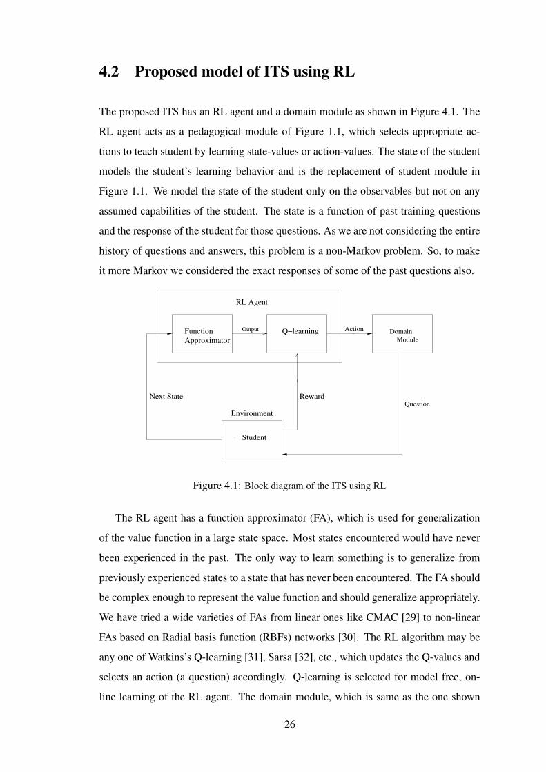
The proposed ITS has an RL agent and a domain module as shown in Figure 4.1. The

RL agent acts as a pedagogical module of Figure 1.1, which selects appropriate ac-

tions to teach student by learning state-values or action-values. The state of the student

models the student’s learning behavior and is the replacement of student module in

Figure 1.1. We model the state of the student only on the observables but not on any

assumed capabilities of the student. The state is a function of past training questions

and the response of the student for those questions. As we are not considering the entire

history of questions and answers, this problem is a non-Markov problem. So, to make

it more Markov we considered the exact responses of some of the past questions also.

Output

ApproximatorFunction Q−learning

Student

RewardNext State

RL Agent

Environment

Domain Action

Question

Module

Figure 4.1: Block diagram of the ITS using RL

The RL agent has a function approximator (FA), which is used for generalization

of the value function in a large state space. Most states encountered would have never

been experienced in the past. The only way to learn something is to generalize from

previously experienced states to a state that has never been encountered. The FA should

be complex enough to represent the value function and should generalize appropriately.

We have tried a wide varieties of FAs from linear ones like CMAC [29] to non-linear

FAs based on Radial basis function (RBFs) networks [30]. The RL algorithm may be

any one of Watkins’s Q-learning [31], Sarsa [32], etc., which updates the Q-values and

selects an action (a question) accordingly. Q-learning is selected for model free, on-

line learning of the RL agent. The domain module, which is same as the one shown

26

in Figure 1.1, contains questions from a topic that is to be taught to the student, which

should be designed according to the teaching topic under consideration.

The reward is the only feedback from the student to the RL agent. So, the reward

function, which maps the students’ response into a reward signal, should be selected

such that the RL agent gets precise feedback about the student and can take appropriate

teaching action. The teaching process is split into two phases, the training phase and the

testing phase of the student. In testing phase, the student is given a question selected by

the RL agent.A random initial state of the student is considered to take an initial action.

Here, an action of the RL agent corresponds to selecting an appropriate question to the

student according to his need. Typically, each question has multiple options of answers,

among which the student has to select correct answer. A reward to the RL agent is

obtained from the student’s response to that question.

In the second phase, which is the training phase of the student, the student is given

the correct answer to the tested question and the state of the student is updated. Then

these state and reward are used to take subsequent actions. This on-line testing and

training processes are continued for some pre-specified number of questions, which is

called an episode. Following is a step-wise description of the processes in the proposed

ITS:

Algorithm 1 Pseudocode of teaching process with the ITSfor each episode do

Select a random initial state, s, reward, rtInitialize Q-values, randomlyfor each question do

//Testing phase of the studentSelect an action, a (or question) from Q(s,a), ε-greedilyTest the student with the questionObtain the reward from the response of student//Training phase of the studentTrain the student with the same questionUpdate the state of the student, Q-values and weights

end forend for

27

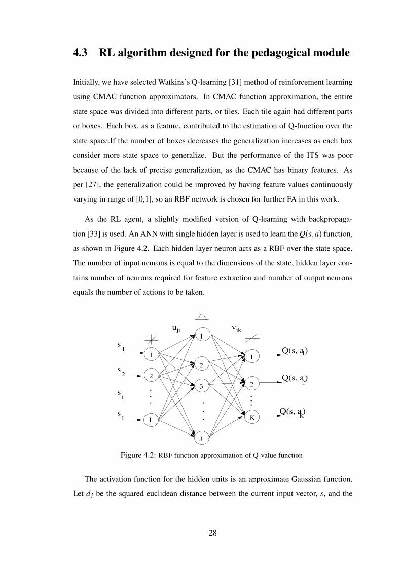
4.3 RL algorithm designed for the pedagogical module

Initially, we have selected Watkins’s Q-learning [31] method of reinforcement learning

using CMAC function approximators. In CMAC function approximation, the entire

state space was divided into different parts, or tiles. Each tile again had different parts

or boxes. Each box, as a feature, contributed to the estimation of Q-function over the

state space.If the number of boxes decreases the generalization increases as each box

consider more state space to generalize. But the performance of the ITS was poor

because of the lack of precise generalization, as the CMAC has binary features. As

per [27], the generalization could be improved by having feature values continuously

varying in range of [0,1], so an RBF network is chosen for further FA in this work.

As the RL agent, a slightly modified version of Q-learning with backpropaga-

tion [33] is used. An ANN with single hidden layer is used to learn the Q(s,a) function,

as shown in Figure 4.2. Each hidden layer neuron acts as a RBF over the state space.

The number of input neurons is equal to the dimensions of the state, hidden layer con-

tains number of neurons required for feature extraction and number of output neurons

equals the number of actions to be taken.

... ...

...

1

2

i

I

1

2

I

1

2

K

J

3

2

1

s

s

s

v

s)Q(s, a 1

Q(s, a

Q(s, a

)

)

2

K

jkjiu

Figure 4.2: RBF function approximation of Q-value function

The activation function for the hidden units is an approximate Gaussian function.

Let d j be the squared euclidean distance between the current input vector, s, and the

28

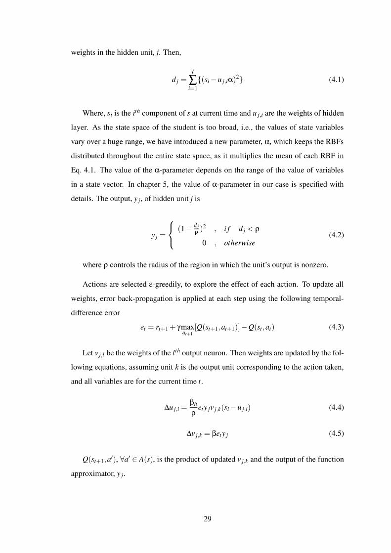
weights in the hidden unit, j. Then,

d j =I

∑i=1(si−u j,iα)2 (4.1)

Where, si is the ith component of s at current time and u j,i are the weights of hidden

layer. As the state space of the student is too broad, i.e., the values of state variables

vary over a huge range, we have introduced a new parameter, α, which keeps the RBFs

distributed throughout the entire state space, as it multiplies the mean of each RBF in

Eq. 4.1. The value of the α-parameter depends on the range of the value of variables

in a state vector. In chapter 5, the value of α-parameter in our case is specified with

details. The output, y j, of hidden unit j is

y j =

(1− d jρ )2 , i f d j < ρ

0 , otherwise(4.2)

where ρ controls the radius of the region in which the unit’s output is nonzero.

Actions are selected ε-greedily, to explore the effect of each action. To update all

weights, error back-propagation is applied at each step using the following temporal-

difference error

et = rt+1 + γmaxat+1

[Q(st+1,at+1)]−Q(st,at) (4.3)

Let v j,l be the weights of the lth output neuron. Then weights are updated by the fol-

lowing equations, assuming unit k is the output unit corresponding to the action taken,

and all variables are for the current time t.

∆u j,i =βhρ

ety jv j,k(si−u j,i) (4.4)

∆v j,k = βety j (4.5)

Q(st+1,a′), ∀a′ ∈ A(s), is the product of updated v j,k and the output of the function

approximator, y j.

29

4.4 Issues

With the application of RL to the ITS, some more issues than we discussed in section 1.4

will arise. This section discuses some of those issues in brief, while section 5.6 presents

a detailed analysis of the issues we have addressed empirically.

4.4.1 Reward function

Reward is the only feedback through which the RL agent should evaluate the student’s

behavior and should take a teaching action. RL updates a policy with this reward, to

select an action that maximizes the future reward. A reward function maps the students’

answer into a scalar value, reward. So, the reward function should be selected such that

the RL agent can evaluate the student precisely and can take appropriate further teaching

actions.

4.4.2 State representation

RL algorithms depend on the Markov assumption as said in section 3.1.1 to estimate

the rewards. This needs a state signal to provide sufficient information to determine the

effects of all actions. So, the information gathered through the effect of an action a in

a given state s, represented as Q(s,a), cannot be directly transferred to similar states or

actions. The cost of a RL algorithm in a general problem is Ω(ns na), where ns is the

number of states and na is the number of actions. This is because, each action has to be

tried at least once in each state. As the state is defined by the observed combination of

features that represent knowledge of the student, we have that the potential number of

states is ns = 2n f , with n f the number of features. So, we have that Ω(ns na)= Ω(2n f na),

which is exponential in the number of features. If the number of features moves towards

high then non-generalizing RL becomes impractical for realistic problems like Intelli-

gent Tutoring Systems. This is the known as curse of dimensionality introduced in [34].

So, the state representations should have optimal number of features that can model a

students’ knowledge on the topic being taught.

30

4.4.3 Action set

We have, Ω(ns na) = Ω(2n f na), which implies that the cost of RL algorithm also de-

pends on the number of actions, na. The cost of the algorithm increases with the number

of actions to be taken. So, the action set should be compact for the better performance

of the RL algorithm.

4.5 Artificial neural networks as simulated student

Cohen has shown that an ANN could be used to simulate the autistic students, with sim-

ilarities in selective attention and generalization deficits. There are two type of models

suggested by him in [35] and [36]. The models were based on neuropathalogical stud-

ies which suggested that the affected persons have either too few or too many neuronal

connections in various regions of their brain. In that work, it was shown that an ANN

having too few neuronal connections simulated the autistic student in terms of inferior

discrimination of input patterns, where the model was taught to discriminate two groups

in the input testing set. But, too many connections produced excellent discrimination

but inferior generalization because of overemphasis on details unique to the training set.

In two layer networks, one of the most important issues in network construction

is the number of connections needed to store a distributed representation of a given

association. The network can learn different associations if all inputs and outputs are

completely interconnected. There is a greater chance that the new association will be

similar to already stored associations as the number of associations to be learned in-

creases. Already learned patterns will be ”forgotten” if the network adjusts its weight

in order to learn these similar patterns. So, having “too many” connections in a simple

one or two layer network can lead to a problem with storage capacity. If the number of

connections or neurons are “too few” then the network over fits the data which is due to

lack of generalization.

In that work, he has mentioned different methods of modeling autistic students with

ANNs, two of them we used for experimenting. One method is to have more number

of neurons in the hidden layer than required for the capturing the information in the

31

input data and the other method is to take random inputs of the ANN which are highly

correlated to the output. This correlation is analogous to the teacher, providing hints to

the correct answer. According to Cohen, this speeds up learning while causing problems

in generalization, simulating learning behavior in autistic children.

4.5.1 Autism and its effects

While addressing the issues in designing the ITS in the present work, we have validated

the application of this ITS to teach children, both having normal learning abilities and

having autism, through simulation models. Autism is a semantic pragmatic disorder of

development that exists throughout a person’s life [37]. It is sometimes called a devel-

opmental disability, as it usually starts before age three, in the developmental period,

and because it causes delays or problems in many different skills that arise from child-

hood to the adulthood. Many children with autism do make eye contact, especially with

familiar people. But, the eye contact could be less frequent than expected and may

not be used for efficient communication. Along with the deficits, autistic people may

have exceptional learning skills, which could be used by ITS designer to facilitate their

learning.

The main signs and symptoms of autism involve communication, social behavior,

and behaviors concerning objects and routines. People with autism might have prob-

lems talking to others, or they might not want to look others in the eye when talking

to them. They may have to line up their pencils before they can pay attention or they

may say the same sentence again and again to calm down themselves. They may flap

their arms to tell us they are happy, or they might hurt themselves to tell us they are not

happy. Some people with autism never learn how to talk.

These behavior not only makes life difficult for people who have autism, but also

makes it difficult for their families, their health care providers, their teachers, and any-

one who comes in contact with them. An ITS can serve the purpose of human teachers

to teach such type of students. Through the ITS these children would not find difficulty

of eye contact, communication and other difficulties that they face with human teachers.

In brief, the two methods that Cohen had proposed to simulated learning behavior

32

in children are:

• To have more number of neurons in the hidden layer than required for the captur-ing the information in the input data.

• To have random additional inputs, which are highly correlated to the output of theANN.

In chapter 5, we have presented the experiments of the proposed ITS on a simulated

student. We have also discussed the issues by presenting the performance of the ITS

with different domain knowledge bases.

33

CHAPTER 5

Evaluation of the proposed ITS

The goal of this work was to develop an ITS, capable of adapting to large deviations

from normal learning behavior. So, we have simulated models of both autistic stu-

dent [35] and normal student by selecting more number of neurons in the hidden layer

than that required for capturing the information in the input patterns. The ITS has been

evaluated using these simulated models. For the simplification of explaining results,

hereafter, we will consider ANN models of the students as:

• Type-I : normal behavior

• Type-II : autistic behavior with less number of hidden layer neurons than Type-I,

• Type-III: autistic behavior with more number of hidden layer neurons than Type-I,

• Type-IV : autistic behavior with irrelevant random inputs.

5.1 Classification Problem

Experiments were performed, with the proposed ITS, to teach pattern classification

problems to the ANN models of both autistic (Type-II and Type-III) and normal (Type-

I) students. In our case, the pattern classification problem is that the ANN has to classify

the pattern (question) presented at its input. This problem has been chosen to validate

the proposed ITS, though it doesn’t have any relevance in teaching human students.

Appropriate question banks should be developed to teach human students in real-world

situations. A brief discussion on the real-world situation is in chapter 6.

Experiments were also conducted on different data bases i.e., different pattern clas-

sification problems to validate the adaptability of the system to different data sets

and, simultaneously, with different environments (students). Sections 5.2, 5.3, and 5.4

present in detail the experiments done with four, three and five classes, respectively, and

results obtained thereby.

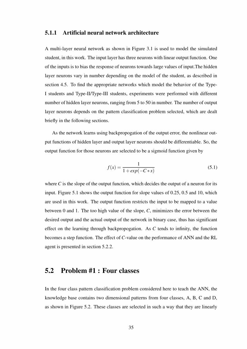
5.1.1 Artificial neural network architecture

A multi-layer neural network as shown in Figure 3.1 is used to model the simulated

student, in this work. The input layer has three neurons with linear output function. One

of the inputs is to bias the response of neurons towards large values of input.The hidden

layer neurons vary in number depending on the model of the student, as described in

section 4.5. To find the appropriate networks which model the behavior of the Type-

I students and Type-II/Type-III students, experiments were performed with different

number of hidden layer neurons, ranging from 5 to 50 in number. The number of output

layer neurons depends on the pattern classification problem selected, which are dealt

briefly in the following sections.

As the network learns using backpropogation of the output error, the nonlinear out-

put functions of hidden layer and output layer neurons should be differentiable. So, the

output function for those neurons are selected to be a sigmoid function given by

f (x) =1

1+ exp(−C ∗ x) (5.1)

where C is the slope of the output function, which decides the output of a neuron for its

input. Figure 5.1 shows the output function for slope values of 0.25, 0.5 and 10, which

are used in this work. The output function restricts the input to be mapped to a value

between 0 and 1. The too high value of the slope, C, minimizes the error between the

desired output and the actual output of the network in binary case, thus has significant

effect on the learning through backpropogation. As C tends to infinity, the function

becomes a step function. The effect of C-value on the performance of ANN and the RL

agent is presented in section 5.2.2.

5.2 Problem #1 : Four classes

In the four class pattern classification problem considered here to teach the ANN, the

knowledge base contains two dimensional patterns from four classes, A, B, C and D,

as shown in Figure 5.2. These classes are selected in such a way that they are linearly

35

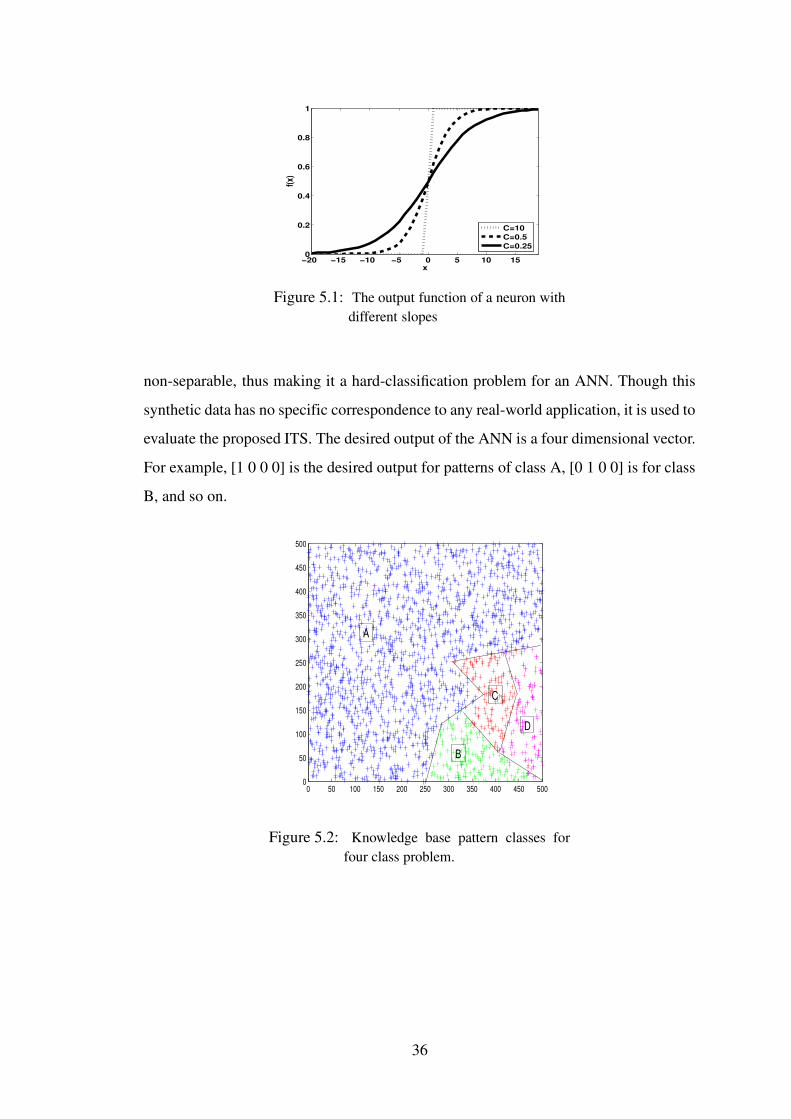
−20 −15 −10 −5 0 5 10 150

0.2

0.4

0.6

0.8

1

x

f(x)

C=10C=0.5C=0.25

Figure 5.1: The output function of a neuron withdifferent slopes

non-separable, thus making it a hard-classification problem for an ANN. Though this

synthetic data has no specific correspondence to any real-world application, it is used to

evaluate the proposed ITS. The desired output of the ANN is a four dimensional vector.

For example, [1 0 0 0] is the desired output for patterns of class A, [0 1 0 0] is for class

B, and so on.

0 50 100 150 200 250 300 350 400 450 5000

50

100

150

200

250

300

350

400

450

500

A

C

B

D

Figure 5.2: Knowledge base pattern classes forfour class problem.

36

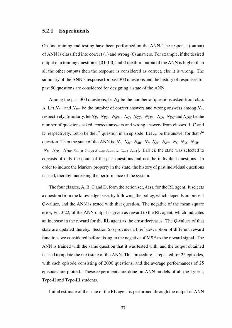
5.2.1 Experiments

On-line training and testing have been performed on the ANN. The response (output)

of ANN is classified into correct (1) and wrong (0) answers. For example, if the desired

output of a training question is [0 0 1 0] and if the third output of the ANN is higher than

all the other outputs then the response is considered as correct, else it is wrong. The

summary of the ANN’s response for past 300 questions and the history of responses for

past 50 questions are considered for designing a state of the ANN.

Among the past 300 questions, let NA be the number of questions asked from class

A. Let NAC and NAW be the number of correct answers and wrong answers among NA,

respectively. Similarly, let NB, NBC, NBW , NC, NCC, NCW , ND, NDC and NDW be the

number of questions asked, correct answers and wrong answers from classes B, C and

D, respectively. Let xi be the ith question in an episode. Let zi, be the answer for that ith

question. Then the state of the ANN is [NA NAC NAW NB NBC NBW NC NCC NCW

ND NDC NDW xi−50 zi−50 xi−49 zi−49... xi−1 zi−1]. Earlier, the state was selected to

consists of only the count of the past questions and not the individual questions. In

order to induce the Markov property in the state, the history of past individual questions

is used, thereby increasing the performance of the system.

The four classes, A, B, C and D, form the action set, A(s), for the RL agent. It selects

a question from the knowledge base, by following the policy, which depends on present

Q-values, and the ANN is tested with that question. The negative of the mean square

error, Eq. 3.22, of the ANN output is given as reward to the RL agent, which indicates

an increase in the reward for the RL agent as the error decreases. The Q-values of that

state are updated thereby. Section 5.6 provides a brief description of different reward

functions we considered before fixing to the negative of MSE as the reward signal. The

ANN is trained with the same question that it was tested with, and the output obtained

is used to update the next state of the ANN. This procedure is repeated for 25 episodes,

with each episode consisting of 2000 questions, and the average performances of 25

episodes are plotted. These experiments are done on ANN models of all the Type-I,

Type-II and Type-III students.

Initial estimate of the state of the RL agent is performed through the output of ANN

37

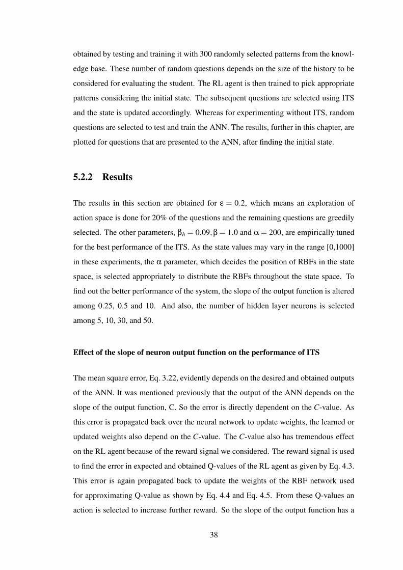
obtained by testing and training it with 300 randomly selected patterns from the knowl-

edge base. These number of random questions depends on the size of the history to be

considered for evaluating the student. The RL agent is then trained to pick appropriate

patterns considering the initial state. The subsequent questions are selected using ITS

and the state is updated accordingly. Whereas for experimenting without ITS, random

questions are selected to test and train the ANN. The results, further in this chapter, are

plotted for questions that are presented to the ANN, after finding the initial state.

5.2.2 Results

The results in this section are obtained for ε = 0.2, which means an exploration of

action space is done for 20% of the questions and the remaining questions are greedily

selected. The other parameters, βh = 0.09,β = 1.0 and α = 200, are empirically tuned

for the best performance of the ITS. As the state values may vary in the range [0,1000]

in these experiments, the α parameter, which decides the position of RBFs in the state

space, is selected appropriately to distribute the RBFs throughout the state space. To

find out the better performance of the system, the slope of the output function is altered

among 0.25, 0.5 and 10. And also, the number of hidden layer neurons is selected

among 5, 10, 30, and 50.

Effect of the slope of neuron output function on the performance of ITS

The mean square error, Eq. 3.22, evidently depends on the desired and obtained outputs

of the ANN. It was mentioned previously that the output of the ANN depends on the

slope of the output function, C. So the error is directly dependent on the C-value. As

this error is propagated back over the neural network to update weights, the learned or

updated weights also depend on the C-value. The C-value also has tremendous effect

on the RL agent because of the reward signal we considered. The reward signal is used

to find the error in expected and obtained Q-values of the RL agent as given by Eq. 4.3.

This error is again propagated back to update the weights of the RBF network used

for approximating Q-value as shown by Eq. 4.4 and Eq. 4.5. From these Q-values an

action is selected to increase further reward. So the slope of the output function has a

38

significant effect on the decisions of an RL agent too, which are shown empirically in

Figure 5.3.

0 500 1000 1500 20000

10

20

30

40

50

60

70

80

90

Question Number

Perc

entag

e Clas

sifica

tion

L.R: 0.2; C: 0.25; Hidd: 5WithITSWithoutITS

0 500 1000 1500 20000

10

20

30

40

50

60

70

80

90

Question Number

Perc

entag

e Clas

sifica

tion

L.R: 0.2; C: 0.5; Hidd: 5WithITSWithoutITS

(a) (b)

0 500 1000 1500 20000

10

20

30

40

50

60

70

80

90

Question Number

Perc

entag

e Clas

sifica

tion

L.R: 0.2; C: 10; Hidd: 5WithITSWithoutITS

0 500 1000 1500 20000

10

20

30

40

50

60

70

80

90

Question Number

Perc

entag

e Clas

sifica

tion

L.R: 0.2; C: 50; Hidd: 5WithITSWithoutITS

(c) (d)

Figure 5.3: The effect of slope (C) of the output of neuron on the classification performancesof the ANN when taught with ITS and without ITS, with 5 hidden layer neurons(Hidd) and learning rate (L.R) of 0.2. Classification performances for (a) C =0.25, (b) C = 0.5, (c) C = 10, (d) C = 50.

Performance of the ANN, without ITS, is not affecting significantly by the change in

the C-value, but it is observed that the C-value has tremendous effect on the performance

of the RL agent. It can be seen in the curves that the degradation of the performance

of ANN is more when taught with ITS. This could be because of the actions selected

by the RL agent are not contributing to the ”learning” of the ANN for such higher C-

values. The improvement in the performance of ANN, when patterns are selected using

the ITS, is because of the sequence of the questions that the ITS is selecting. A detailed

experimental analysis on this is presented later in this section.

Figure 5.4 is the zoomed-in version of Figure 5.3, to analyze the behavior of the

ANN, when taught with ITS and without ITS, for first 300 questions. It is observed that

39

0 50 100 150 200 250 3000

10

20

30

40

50

60

70

80

90

Question Number

Perc

entag

e Clas

sifica

tion

L.R: 0.2; C: 0.25; Hidd: 5WithITSWithoutITS

0 50 100 150 200 250 3000

10

20

30

40

50

60

70

80

90

Question Number

Perc

entag

e Clas

sifica

tion

L.R: 0.2; C: 0.5; Hidd: 5WithITSWithoutITS

(a) (b)

0 50 100 150 200 250 3000

10

20

30

40

50

60

70

80

90

Question Number

Perc

entag

e Clas

sifica

tion

L.R: 0.2; C: 10; Hidd: 5WithITSWithoutITS

0 50 100 150 200 250 3000

10

20

30

40

50

60

70

80

90

Question Number

Perc

entag

e Clas

sifica

tion

L.R: 0.2; C: 50; Hidd: 5WithITSWithoutITS

(c) (d)

Figure 5.4: Classification performances of ANN for first three hundred questions with, (a) C= 0.25, (b) C = 0.5, (c) C = 10, (d) C = 50.

the performance of the ITS is same for first 50 questions for different C-values, but the

subsequent selection of questions are being affected as the C-value changes.

Considering the better performance of the ITS for C-value of 10, it is selected for

experimenting and analysis of the ITS for this knowledge base, further in this thesis.

Effect of the learning rate of ANN on the performance of the ITS

Figure 5.6 shows the performance of the ANN for different learning rates. For cali-

bration of learning rate, the figure is shown for 5 number of hidden layer processing

unit, later in this section we will chose the appropriate number of hidden layer neurons

that will model Type-I, Type-II, and Type-III students behavior. It is observed in the

figure that the ANN with learning rate of 0.2 is performing poorly, without ITS for this

knowledge base, when compared to the performance with other learning rates. So, in

order to validate the proposed ITS and to prove the performance of ITS even with worst

40

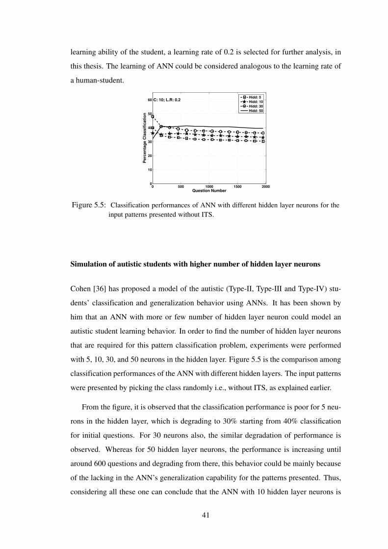
learning ability of the student, a learning rate of 0.2 is selected for further analysis, in

this thesis. The learning of ANN could be considered analogous to the learning rate of

a human-student.

0 500 1000 1500 20000

10

20

30

40

50

60

Question Number

Perc

enta

ge C

lass

ifica

tion

C: 10; L.R: 0.2 Hidd: 5Hidd: 10Hidd: 30Hidd: 50

Figure 5.5: Classification performances of ANN with different hidden layer neurons for theinput patterns presented without ITS.

Simulation of autistic students with higher number of hidden layer neurons

Cohen [36] has proposed a model of the autistic (Type-II, Type-III and Type-IV) stu-

dents’ classification and generalization behavior using ANNs. It has been shown by

him that an ANN with more or few number of hidden layer neuron could model an

autistic student learning behavior. In order to find the number of hidden layer neurons

that are required for this pattern classification problem, experiments were performed

with 5, 10, 30, and 50 neurons in the hidden layer. Figure 5.5 is the comparison among

classification performances of the ANN with different hidden layers. The input patterns

were presented by picking the class randomly i.e., without ITS, as explained earlier.

From the figure, it is observed that the classification performance is poor for 5 neu-

rons in the hidden layer, which is degrading to 30% starting from 40% classification

for initial questions. For 30 neurons also, the similar degradation of performance is

observed. Whereas for 50 hidden layer neurons, the performance is increasing until

around 600 questions and degrading from there, this behavior could be mainly because

of the lacking in the ANN’s generalization capability for the patterns presented. Thus,

considering all these one can conclude that the ANN with 10 hidden layer neurons is

41

giving Type-I performance because the performance of this ANN is not degrading at

any stage, whereas ANN with 5 and 50 neurons are showing Type-II and Type-III per-

formance, which could be considered as models of an autistic student as per Cohen [36].

Analysis of the performance of ITS

The proposed ITS is used to teach the classification problem to the above specified

models of both Type-I and autistic (Type-II and Type-III) students. From Figure 5.7, it is

evident that the performance of the ANN when patterns are presented is improved when

compared to without ITS in all the three cases of the number of hidden layer neurons.

But the questions that could arise here are, what is the reason for this improvement in

the performance? and what is the learning in ITS?

These questions can be answered by looking into the Figure 5.8, which shows the

histogram of action sequence from same class. Generally, the classification rate of an

artificial neural network depends on the way the input patterns are presented. As it

was explained earlier in section 3.2, the weights of ANN are updated depending on the

output error, which again depends on the input patterns. In Figure 5.8.(a), the white

bars indicate the histogram of average length of the sequence of actions taken from the

same class when selected randomly, i.e., without ITS, for the slope of output function of

neurons, C=10, learning rate, L.R=0.3 and the number of hidden layer neurons, Hidd=5.

It can be observed that the length of the sequence is 1 for nearly 1100 average number

of questions. And it is also observed that there are no sequence of questions from same

class more than a length of 10. Whereas, the black bar indicates the same histogram

for the questions selected by the ITS. There are long sequence of questions from the

same class most of the times. Figure 5.8.(b) shows that the length of the sequence also

exists between 46-70. As the patterns are presented to the ANN from the same class

most of the time, continuously by the ITS, the performance of the ANN has improved

significantly.

From the same figures, it is can be concluded that ITS is learning to present the pat-

terns appropriately to increase the performance of the student (ANN). But, there could

be a possibility of the ITS sticking in a local optima, where the ITS selects questions

42

most of the time from same class. Figure 5.7.(b), (d) and (f) show that this is not hap-

pening in this case. It is evident from these figures that the over all actions selected by

the ITS is nearly uniform, which is the desired behavior of an ITS.

Simulation of autistic student with random inputs to the ANN

To check the adaptability of the ITS with different students, another model of the autistic

students behavior, proposed by Cohen [35], is also used to experiment with the same

ITS. In this model, he had proposed to take random inputs (Type-IV) for an ANN, which

are irrelevant to the data set being used. Experiments have been conducting for 1, 3, 5

and 10 random inputs for the neural network. The random inputs were generated with

40% correlation to the output. This patterns with random inputs were used for training

the ANN and the patterns without these random inputs (original data set) are used for

testing. In the previous sub-section, it was mentioned that an ANN with 10 number of

hidden layer neurons is “behaving normally” for the data set, when compared to other

number of neurons. So, to simulate an autistic student with random inputs, 10 neurons

in the hidden layer of the neural network is used.

Figure 5.9 shows the performances of ITS and ANN. It is proved with the results

that the ITS is adapting itself to the new environments and improving the performance

of the students.

In the following sections, the results for different data sets is presented, which would

prove that the same ITS can be used for different data sets too. This chapter ends with

a detailed discussion on the empirical issues related to the development of an ITS using

RL.

43

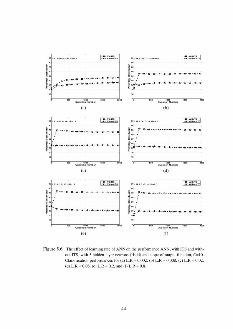
0 500 1000 1500 20000

10

20

30

40

50

60

70

80

90

Question Number

Perc

entag

e Clas

sifica

tion

L.R: 0.002; C: 10; Hidd: 5WithITSWithoutITS

0 500 1000 1500 20000

10

20

30

40

50

60

70

80

90

Question Number

Perc

entag

e Clas

sifica

tion

L.R: 0.008; C: 10; Hidd: 5WithITSWithoutITS

(a) (b)

0 500 1000 1500 20000

10

20

30

40

50

60

70

80

90

Question Number

Perc

entag

e Clas

sifica

tion

L.R: 0.02; C: 10; Hidd: 5WithITSWithoutITS

0 500 1000 1500 20000

10

20

30

40

50

60

70

80

90

Question Number

Perc

entag

e Clas

sifica

tion

L.R: 0.08; C: 10; Hidd: 5WithITSWithoutITS

(c) (d)

0 500 1000 1500 20000

10

20

30

40

50

60

70

80

90

Question Number

Perc

entag

e Clas

sifica

tion

L.R: 0.2; C: 10; Hidd: 5WithITSWithoutITS

0 500 1000 1500 20000

10

20

30

40

50

60

70

80

90

Question Number

Perc

entag

e Clas

sifica

tion

L.R: 0.8; C: 10; Hidd: 5WithITSWithoutITS

(e) (f)

Figure 5.6: The effect of learning rate of ANN on the performance ANN, with ITS and with-out ITS, with 5 hidden layer neurons (Hidd) and slope of output function, C=10.Classification performances for (a) L.R = 0.002, (b) L.R = 0.008, (c) L.R = 0.02,(d) L.R = 0.08, (e) L.R = 0.2, and (f) L.R = 0.8.

44

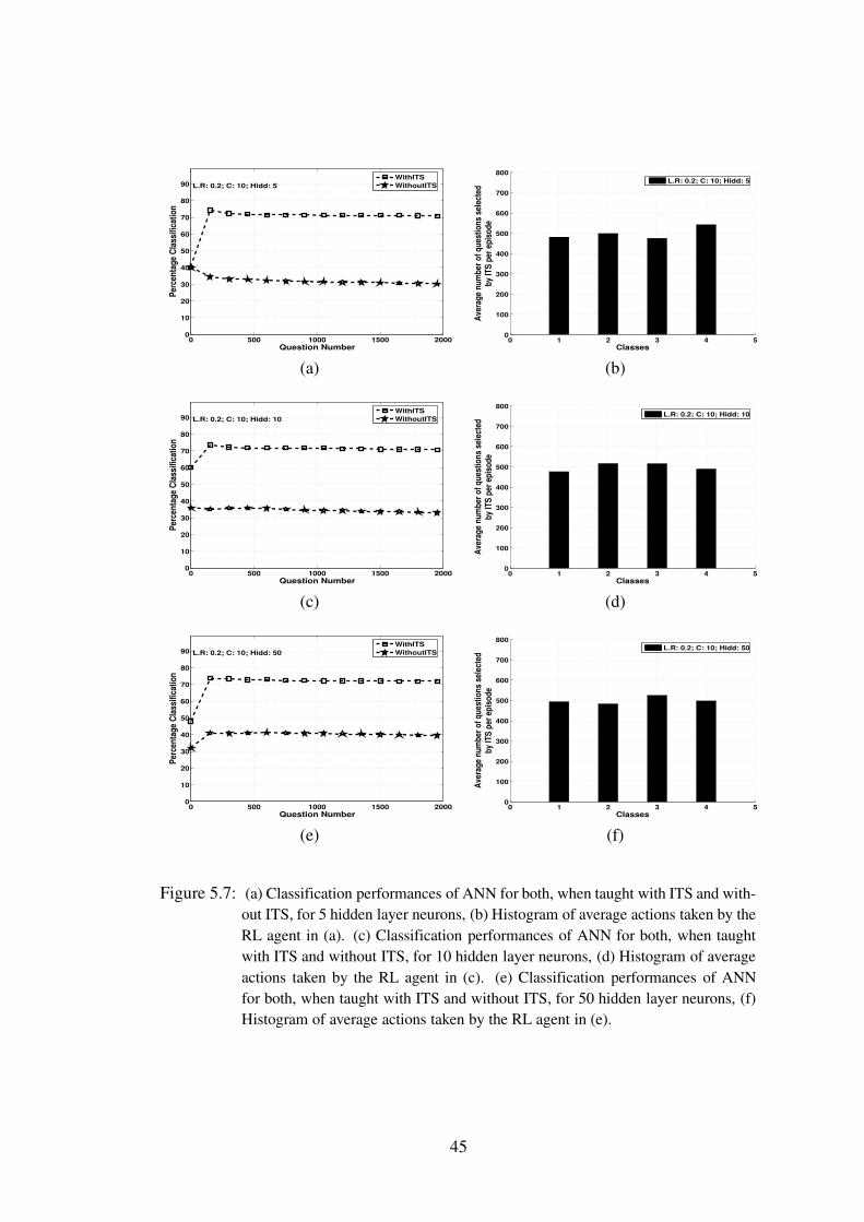
0 500 1000 1500 20000

10

20

30

40

50

60

70

80

90

Question Number

Perc

entag

e Clas

sifica

tion

L.R: 0.2; C: 10; Hidd: 5WithITSWithoutITS

0 1 2 3 4 50

100

200

300

400

500

600

700

800

Classes

Aver

age n

umbe

r of q

uest

ions

selec

ted

by IT

S pe

r epi

sode

L.R: 0.2; C: 10; Hidd: 5

(a) (b)

0 500 1000 1500 20000

10

20

30

40

50

60

70

80

90

Question Number

Perc

entag

e Clas

sifica

tion

L.R: 0.2; C: 10; Hidd: 10WithITSWithoutITS

0 1 2 3 4 50

100

200

300

400

500

600

700

800

Classes

Aver

age n

umbe

r of q

uest

ions

selec

ted

by IT

S pe

r epi

sode

L.R: 0.2; C: 10; Hidd: 10

(c) (d)

0 500 1000 1500 20000

10

20

30

40

50

60

70

80

90

Question Number

Perc

entag

e Clas

sifica

tion

L.R: 0.2; C: 10; Hidd: 50WithITSWithoutITS

0 1 2 3 4 50

100

200

300

400

500

600

700

800

Classes

Aver

age n

umbe

r of q

uest

ions

selec

ted

by IT

S pe

r epi

sode

L.R: 0.2; C: 10; Hidd: 50

(e) (f)

Figure 5.7: (a) Classification performances of ANN for both, when taught with ITS and with-out ITS, for 5 hidden layer neurons, (b) Histogram of average actions taken by theRL agent in (a). (c) Classification performances of ANN for both, when taughtwith ITS and without ITS, for 10 hidden layer neurons, (d) Histogram of averageactions taken by the RL agent in (c). (e) Classification performances of ANNfor both, when taught with ITS and without ITS, for 50 hidden layer neurons, (f)Histogram of average actions taken by the RL agent in (e).

45

1 2 3−10 11−20 21−30 31−45 46−700

200

400

600

800

1000

Avg. length of a sequence of questions from the same class per episode

Avg.

num

ber o

f occ

uren

ces o

f the

sequ

ence

per

episo

de

C: 10; L.R. : 0.2; Hidd: 5

WithITSWithoutITS

3−10 11−20 21−30 31−45 46−700

5

10

15

Avg. length of a sequence of questions from the same class per episode

Avg.

num

ber o

f occ

uren

ces o

f the

sequ

ence

per

episo

de

C: 10; L.R. : 0.2; Hidd: 5

WithITSWithoutITS

(a) (b)

1 2 3−10 11−20 21−30 31−45 46−700

200

400

600

800

1000

Avg. length of a sequence of questions from the same class per episode

Avg.

num

ber o

f occ

uren

ces o

f the

sequ

ence

per

episo

de

C: 10; L.R. : 0.2; Hidd: 10

WithITSWithoutITS

3−10 11−20 21−30 31−45 46−700

5

10

15

Avg. length of a sequence of questions from the same class per episode

Avg.

num

ber o

f occ

uren

ces o

f the

sequ

ence

per

episo

deC: 10; L.R. : 0.2; Hidd: 10

WithITSWithoutITS

(c) (d)

1 2 3−10 11−20 21−30 31−45 46−700

200

400

600

800

1000

Avg. length of a sequence of questions from the same class per episode

Avg.

num

ber o

f occ

uren

ces o

f the

sequ

ence

per

episo

de

C: 10; L.R. : 0.2; Hidd: 50

WithITSWithoutITS

3−10 11−20 21−30 31−45 46−700

5

10

15

Avg. length of a sequence of questions from the same class per episode

Avg.

num

ber o

f occ

uren

ces o

f the

sequ

ence

per

episo

de

C: 10; L.R. : 0.2; Hidd: 50

WithITSWithoutITS

(e) (f)

Figure 5.8: Histogram of the sequences of actions selected by both RL agent and randomselection, from the same class. (a), (c) and (e) are for hidden layer neurons of 5,10 and 50, respectively. (b), (d) and (f) are the zoomed-in versions of (a), (c) and(e), respectively.

46

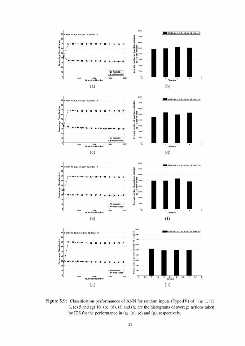
0 500 1000 1500 20000

10

20

30

40

50

60

70

80

90

Question Number

Perc

enta

ge C

lass

ifica

tion

RAND−IN: 1; L.R: 0.2; C: 10; Hidd: 10

WithITSWithoutITS

0 1 2 3 4 50

100

200

300

400

500

600

700

800

Classes

Aver

age

num

ber o

f que

stio

ns s

elec

ted

by IT

S pe

r epi

sode

RAND−IN: 1; L.R: 0.2; C: 10; Hidd: 10

(a) (b)

0 500 1000 1500 20000

10

20

30

40

50

60

70

80

90

Question Number

Perc

enta

ge C

lass

ifica

tion

RAND−IN: 3; L.R: 0.2; C: 10; Hidd: 10

WithITSWithoutITS

0 1 2 3 4 50

100

200

300

400

500

600

700

800

Classes

Aver

age

num

ber o

f que

stio

ns s

elec

ted

by IT

S pe

r epi

sode

RAND−IN: 3; L.R: 0.2; C: 10; Hidd: 10

(c) (d)

0 500 1000 1500 20000

10

20

30

40

50

60

70

80

90

Question Number

Perc

enta

ge C

lass

ifica

tion

RAND−IN: 5; L.R: 0.2; C: 10; Hidd: 10

WithITSWithoutITS

0 1 2 3 4 50

100

200

300

400

500

600

700

800

Classes

Aver

age

num

ber o

f que

stio

ns s

elec

ted

by IT

S pe

r epi

sode

RAND−IN: 5; L.R: 0.2; C: 10; Hidd: 10

(e) (f)

0 500 1000 1500 20000

10

20

30

40

50

60

70

80

90

Question Number

Perc

enta

ge C

lass

ifica

tion

RAND−IN: 10; L.R: 0.2; C: 10; Hidd: 10

WithITSWithoutITS

0 0.5 1 1.5 2 2.5 3 3.5 4 4.5 50

100

200

300

400

500

600

700

800

900

Classes

Aver

age

num

ber o

f que

stio

ns s

elec

ted

by IT

S pe

r epi

sode RAND−IN: 10; L.R: 0.2; C: 10; Hidd: 10

(g) (h)

Figure 5.9: Classification performances of ANN for random inputs (Type-IV) of : (a) 1, (c)3, (e) 5 and (g) 10. (b), (d), (f) and (h) are the histograms of average actions takenby ITS for the performance in (a), (c), (e) and (g), respectively.

47

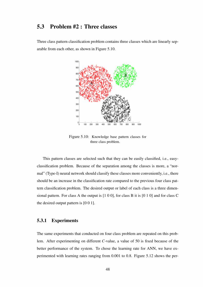
5.3 Problem #2 : Three classes

Three class pattern classification problem contains three classes which are linearly sep-

arable from each other, as shown in Figure 5.10.

0 100 200 300 400 500 600 700 800 900 10000

100

200

300

400

500

600

700

800

900

1000

A

B

C

Figure 5.10: Knowledge base pattern classes forthree class problem.

This pattern classes are selected such that they can be easily classified, i.e., easy-

classification problem. Because of the separation among the classes is more, a “nor-

mal” (Type-I) neural network should classify these classes more conveniently, i.e., there

should be an increase in the classification rate compared to the previous four class pat-

tern classification problem. The desired output or label of each class is a three dimen-

sional pattern. For class A the output is [1 0 0], for class B it is [0 1 0] and for class C

the desired output pattern is [0 0 1].

5.3.1 Experiments

The same experiments that conducted on four class problem are repeated on this prob-

lem. After experimenting on different C-value, a value of 50 is fixed because of the

better performance of the system. To chose the learning rate for ANN, we have ex-

perimented with learning rates ranging from 0.001 to 0.8. Figure 5.12 shows the per-

48

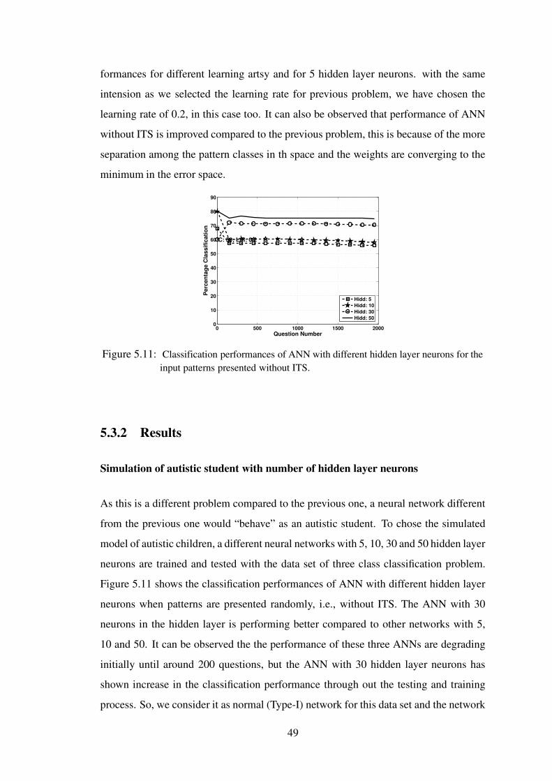
formances for different learning artsy and for 5 hidden layer neurons. with the same

intension as we selected the learning rate for previous problem, we have chosen the

learning rate of 0.2, in this case too. It can also be observed that performance of ANN

without ITS is improved compared to the previous problem, this is because of the more

separation among the pattern classes in th space and the weights are converging to the

minimum in the error space.

0 500 1000 1500 20000

10

20

30

40

50

60

70

80

90

Question Number

Perc

enta

ge C

lass

ifica

tion

C: 50; L.R: 0.2

Hidd: 5Hidd: 10Hidd: 30Hidd: 50

Figure 5.11: Classification performances of ANN with different hidden layer neurons for theinput patterns presented without ITS.

5.3.2 Results

Simulation of autistic student with number of hidden layer neurons

As this is a different problem compared to the previous one, a neural network different

from the previous one would “behave” as an autistic student. To chose the simulated

model of autistic children, a different neural networks with 5, 10, 30 and 50 hidden layer

neurons are trained and tested with the data set of three class classification problem.

Figure 5.11 shows the classification performances of ANN with different hidden layer

neurons when patterns are presented randomly, i.e., without ITS. The ANN with 30

neurons in the hidden layer is performing better compared to other networks with 5,

10 and 50. It can be observed the the performance of these three ANNs are degrading

initially until around 200 questions, but the ANN with 30 hidden layer neurons has

shown increase in the classification performance through out the testing and training

process. So, we consider it as normal (Type-I) network for this data set and the network

49

with 5 and 50 neurons in the hidden layer is considered as “behaving abnormally”

(Type-II and Type-III), so they are considered as the models of autistic children learning

behavior. It can also be observed form Figure 5.5 and Figure 5.11 that the average

classification of the network for four class problem is maximum for 30 hidden layer and

the maximum classification is around 40%. Whereas the classification performance for

three class problem, in this case, is around 60% even with 5 neurons in the hidden layer.

This shows that the patterns in the input data are easily classifiable with less number of

hidden layer neurons if the pattern classes are highly-separated in the space.

Analysis of the performance of ITS on different student models

The performance of ITS on different neural networks with 5, 30 and 50 neurons are pre-

sented in Figure 5.13. There is a little but significant improvement in the performance of

ANN with ITS over the performance without ITS. It can be observed in Figure 5.13 (a),

(c) and (e) that the performances of both ANN models of the Type-I and Type-II/Type-

III children has reached around 90% when compared to 70% without ITS. Figure 5.14

shows the histogram of average lengths sequence of actions taken by ITS for this prob-

lem. The same theory that explained in previous section applies here too. The learning

of the RL agent is evident in these histograms.

Simulation of autistic student with random inputs to the ANN

To validate the performance of the ITS with this data set on different model of stu-

dents as done with previous data set, experiments were repeated on the artificial neural

network with random inputs (Type-IV) of 1, 5 and 10. Figure 5.15 presents the per-

formances of these models with three class classification problem. An improvement of

around 10% is observed in each case.

50

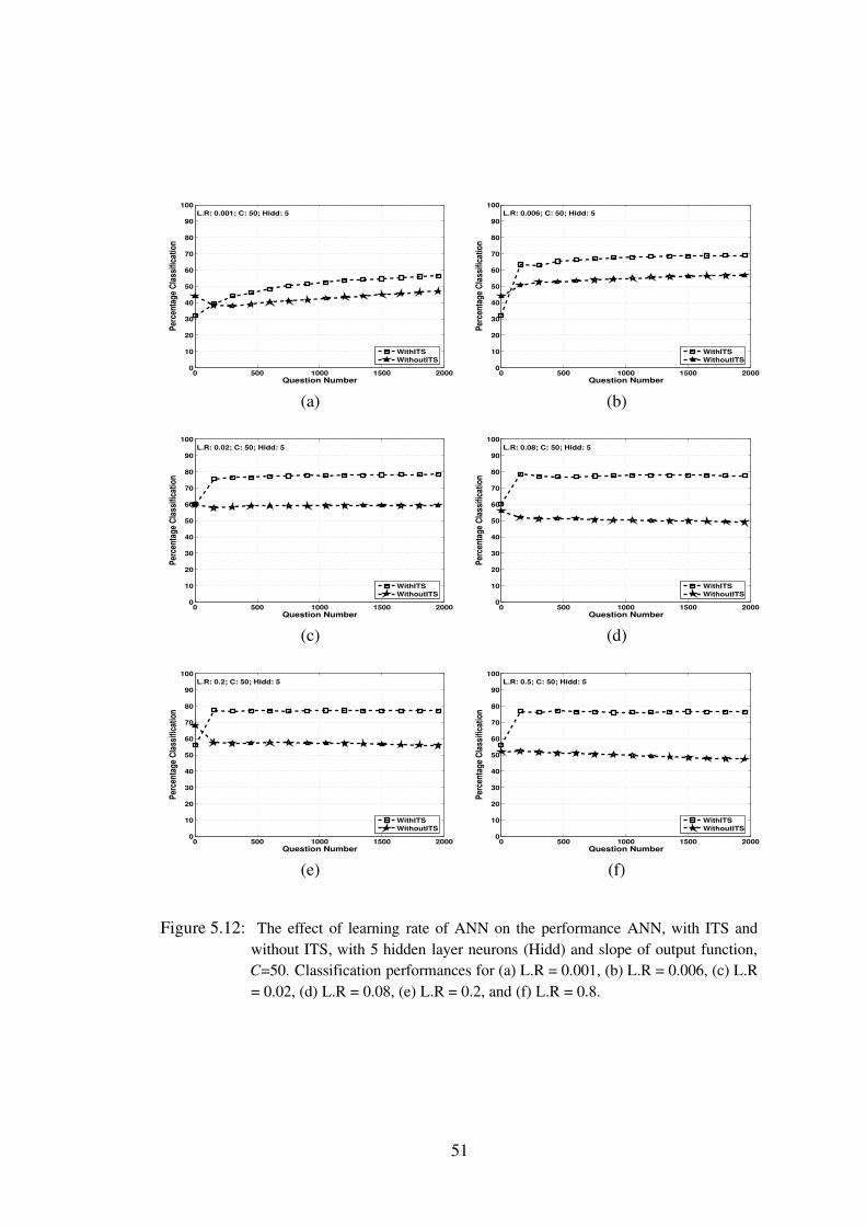
0 500 1000 1500 20000

10

20

30

40

50

60

70

80

90

100

Question Number

Perc

entag

e Clas

sifica

tion

L.R: 0.001; C: 50; Hidd: 5

WithITSWithoutITS

0 500 1000 1500 20000

10

20

30

40

50

60

70

80

90

100

Question Number

Perc

entag

e Clas

sifica

tion

L.R: 0.006; C: 50; Hidd: 5

WithITSWithoutITS

(a) (b)

0 500 1000 1500 20000

10

20

30

40

50

60

70

80

90

100

Question Number

Perc

entag

e Clas

sifica

tion

L.R: 0.02; C: 50; Hidd: 5

WithITSWithoutITS

0 500 1000 1500 20000

10

20

30

40

50

60

70

80

90

100

Question Number

Perc

entag

e Clas

sifica

tion

L.R: 0.08; C: 50; Hidd: 5

WithITSWithoutITS

(c) (d)

0 500 1000 1500 20000

10

20

30

40

50

60

70

80

90

100

Question Number

Perc

entag

e Clas

sifica

tion

L.R: 0.2; C: 50; Hidd: 5

WithITSWithoutITS

0 500 1000 1500 20000

10

20

30

40

50

60

70

80

90

100

Question Number

Perc

entag

e Clas

sifica

tion

L.R: 0.5; C: 50; Hidd: 5

WithITSWithoutITS

(e) (f)

Figure 5.12: The effect of learning rate of ANN on the performance ANN, with ITS andwithout ITS, with 5 hidden layer neurons (Hidd) and slope of output function,C=50. Classification performances for (a) L.R = 0.001, (b) L.R = 0.006, (c) L.R= 0.02, (d) L.R = 0.08, (e) L.R = 0.2, and (f) L.R = 0.8.

51

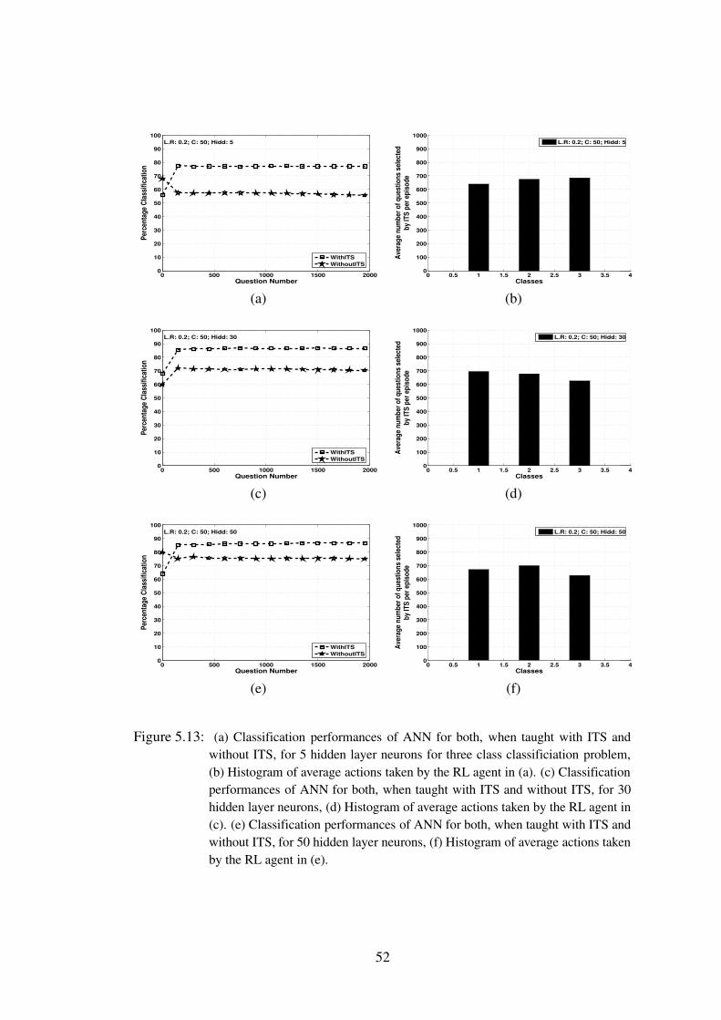
0 500 1000 1500 20000

10

20

30

40

50

60

70

80

90

100

Question Number

Perc

entag

e Clas

sifica

tion

L.R: 0.2; C: 50; Hidd: 5

WithITSWithoutITS

0 0.5 1 1.5 2 2.5 3 3.5 40

100

200

300

400

500

600

700

800

900

1000

Classes

Aver

age n

umbe

r of q

uest

ions

selec

ted

by IT

S pe

r epi

sode

L.R: 0.2; C: 50; Hidd: 5

(a) (b)

0 500 1000 1500 20000

10

20

30

40

50

60

70

80

90

100

Question Number

Perc

entag

e Clas

sifica

tion

L.R: 0.2; C: 50; Hidd: 30

WithITSWithoutITS

0 0.5 1 1.5 2 2.5 3 3.5 40

100

200

300

400

500

600

700

800

900

1000

Classes

Aver

age n

umbe

r of q

uest

ions

selec

ted

by IT

S pe

r epi

sode

L.R: 0.2; C: 50; Hidd: 30

(c) (d)

0 500 1000 1500 20000

10

20

30

40

50

60

70

80

90

100

Question Number

Perc

entag

e Clas

sifica

tion

L.R: 0.2; C: 50; Hidd: 50

WithITSWithoutITS

0 0.5 1 1.5 2 2.5 3 3.5 40

100

200

300

400

500

600

700

800

900

1000

Classes

Aver

age n

umbe

r of q

uest

ions

selec

ted

by IT

S pe

r epi

sode

L.R: 0.2; C: 50; Hidd: 50

(e) (f)

Figure 5.13: (a) Classification performances of ANN for both, when taught with ITS andwithout ITS, for 5 hidden layer neurons for three class classificiation problem,(b) Histogram of average actions taken by the RL agent in (a). (c) Classificationperformances of ANN for both, when taught with ITS and without ITS, for 30hidden layer neurons, (d) Histogram of average actions taken by the RL agent in(c). (e) Classification performances of ANN for both, when taught with ITS andwithout ITS, for 50 hidden layer neurons, (f) Histogram of average actions takenby the RL agent in (e).

52

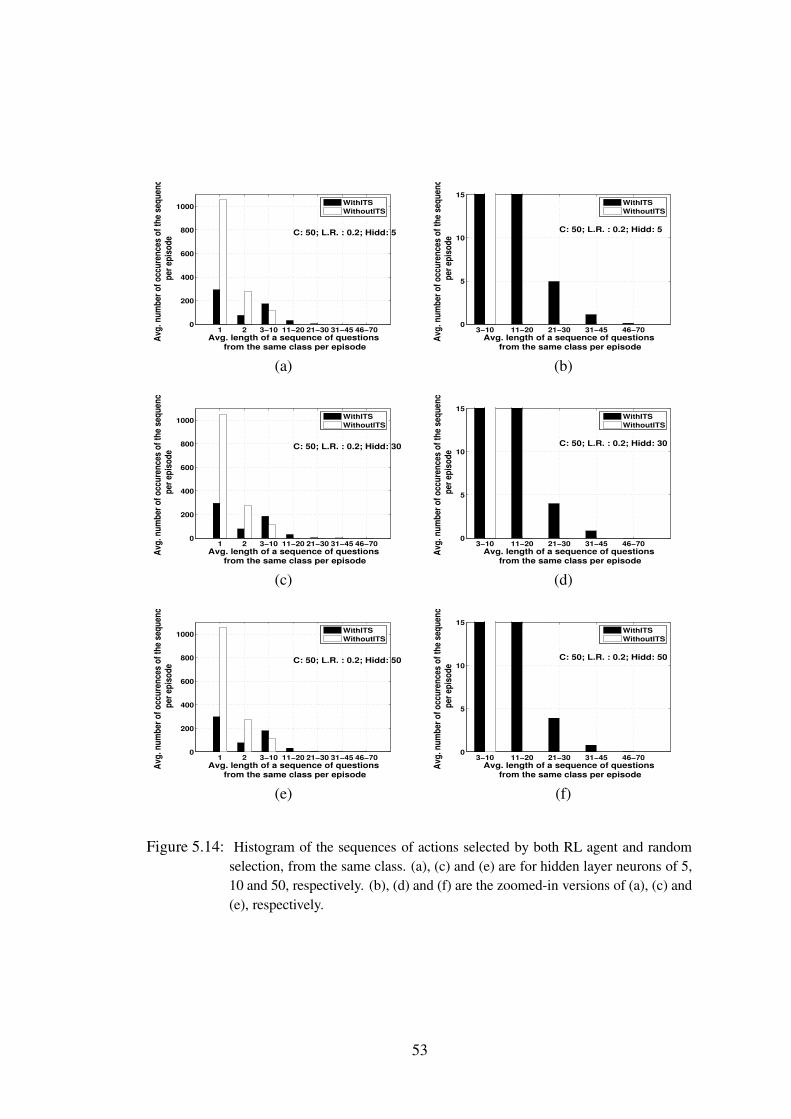
1 2 3−10 11−20 21−30 31−45 46−700

200

400

600

800

1000

Avg. length of a sequence of questions from the same class per episode

Avg.

num

ber o

f occ

uren

ces o

f the

sequ

ence

per

episo

de

C: 50; L.R. : 0.2; Hidd: 5

WithITSWithoutITS

3−10 11−20 21−30 31−45 46−700

5

10

15

Avg. length of a sequence of questions from the same class per episode

Avg.

num

ber o

f occ

uren

ces o

f the

sequ

ence

per

episo

de

C: 50; L.R. : 0.2; Hidd: 5

WithITSWithoutITS

(a) (b)

1 2 3−10 11−20 21−30 31−45 46−700

200

400

600

800

1000

Avg. length of a sequence of questions from the same class per episode

Avg.

num

ber o

f occ

uren

ces o

f the

sequ

ence

per

episo

de

C: 50; L.R. : 0.2; Hidd: 30

WithITSWithoutITS

3−10 11−20 21−30 31−45 46−700

5

10

15

Avg. length of a sequence of questions from the same class per episode

Avg.

num

ber o

f occ

uren

ces o

f the

sequ

ence

per

episo

deC: 50; L.R. : 0.2; Hidd: 30

WithITSWithoutITS

(c) (d)

1 2 3−10 11−20 21−30 31−45 46−700

200

400

600

800

1000

Avg. length of a sequence of questions from the same class per episode

Avg.

num

ber o

f occ

uren

ces o

f the

sequ

ence

per

episo

de

C: 50; L.R. : 0.2; Hidd: 50

WithITSWithoutITS

3−10 11−20 21−30 31−45 46−700

5

10

15

Avg. length of a sequence of questions from the same class per episode

Avg.

num

ber o

f occ

uren

ces o

f the

sequ

ence

per

episo

de

C: 50; L.R. : 0.2; Hidd: 50

WithITSWithoutITS

(e) (f)

Figure 5.14: Histogram of the sequences of actions selected by both RL agent and randomselection, from the same class. (a), (c) and (e) are for hidden layer neurons of 5,10 and 50, respectively. (b), (d) and (f) are the zoomed-in versions of (a), (c) and(e), respectively.

53

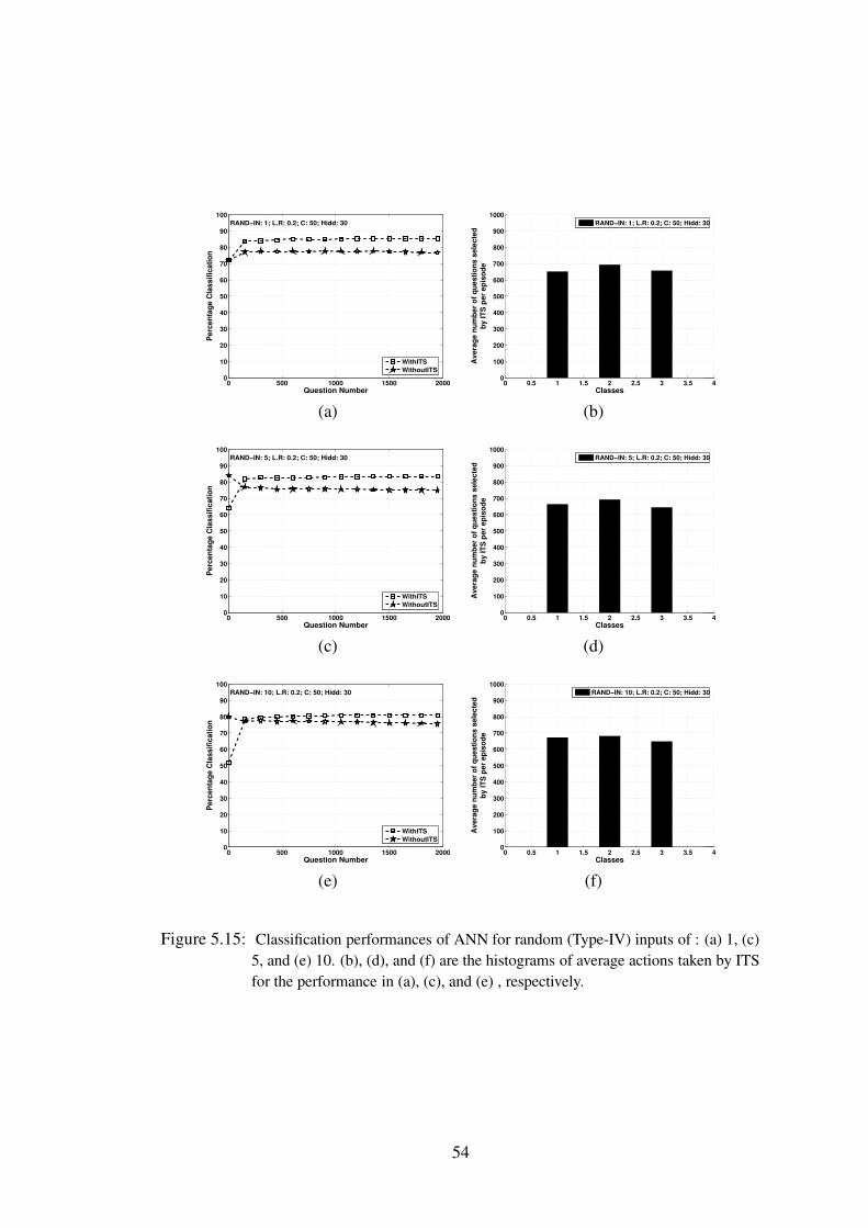
0 500 1000 1500 20000

10

20

30

40

50

60

70

80

90

100

Question Number

Perc

enta

ge C

lass

ifica

tion

RAND−IN: 1; L.R: 0.2; C: 50; Hidd: 30

WithITSWithoutITS

0 0.5 1 1.5 2 2.5 3 3.5 40

100

200

300

400

500

600

700

800

900

1000

Classes

Aver

age

num

ber o

f que

stio

ns s

elec

ted

by IT

S pe

r epi

sode

RAND−IN: 1; L.R: 0.2; C: 50; Hidd: 30

(a) (b)

0 500 1000 1500 20000

10

20

30

40

50

60

70

80

90

100

Question Number

Perc

enta

ge C

lass

ifica

tion

RAND−IN: 5; L.R: 0.2; C: 50; Hidd: 30

WithITSWithoutITS

0 0.5 1 1.5 2 2.5 3 3.5 40

100

200

300

400

500

600

700

800

900

1000

Classes

Aver

age

num

ber o

f que

stio

ns s

elec

ted

by IT

S pe

r epi

sode

RAND−IN: 5; L.R: 0.2; C: 50; Hidd: 30

(c) (d)

0 500 1000 1500 20000

10

20

30

40

50

60

70

80

90

100

Question Number

Perc

enta

ge C

lass

ifica

tion

RAND−IN: 10; L.R: 0.2; C: 50; Hidd: 30

WithITSWithoutITS

0 0.5 1 1.5 2 2.5 3 3.5 40

100

200

300

400

500

600

700

800

900

1000

Classes

Aver

age

num

ber o

f que

stio

ns s

elec

ted

by IT

S pe

r epi

sode

RAND−IN: 10; L.R: 0.2; C: 50; Hidd: 30

(e) (f)

Figure 5.15: Classification performances of ANN for random (Type-IV) inputs of : (a) 1, (c)5, and (e) 10. (b), (d), and (f) are the histograms of average actions taken by ITSfor the performance in (a), (c), and (e) , respectively.

54

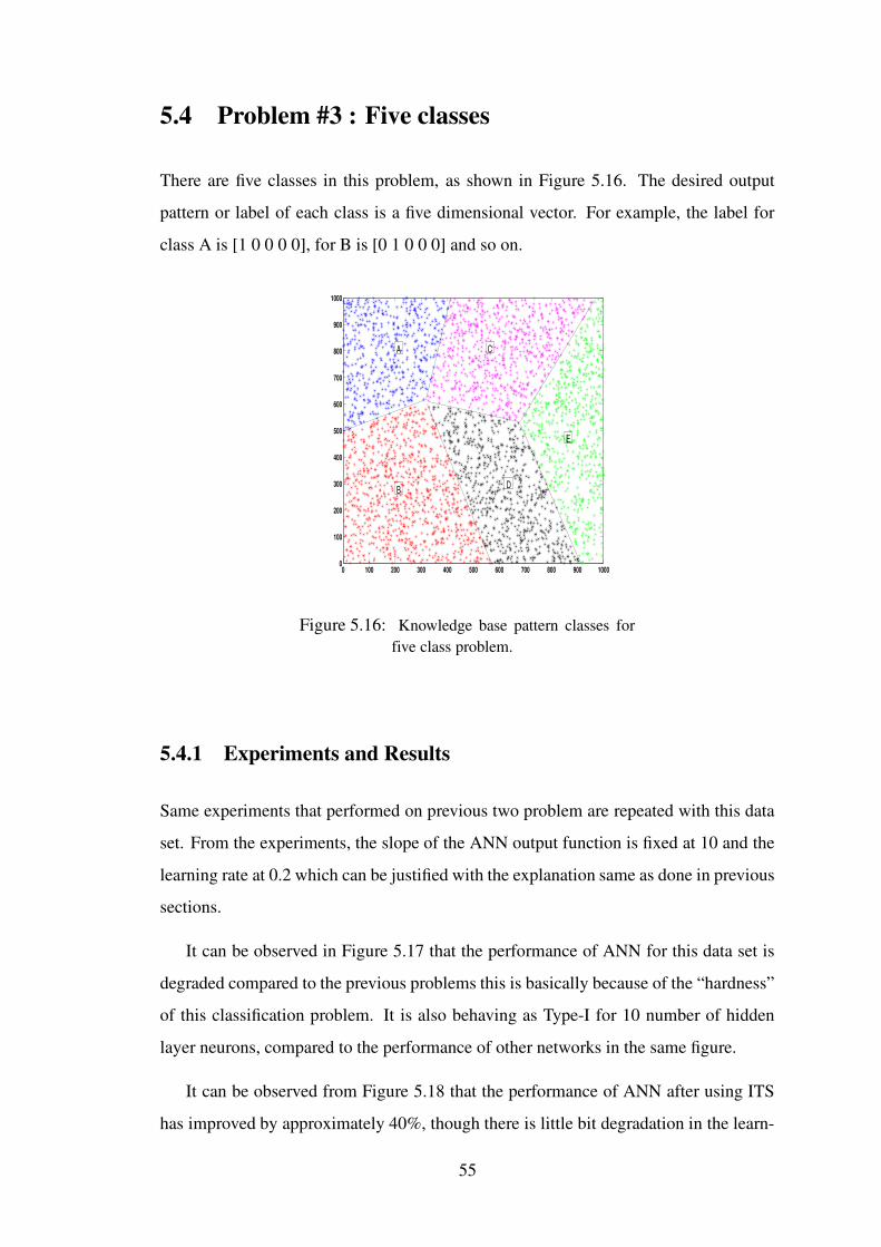
5.4 Problem #3 : Five classes

There are five classes in this problem, as shown in Figure 5.16. The desired output

pattern or label of each class is a five dimensional vector. For example, the label for

class A is [1 0 0 0 0], for B is [0 1 0 0 0] and so on.

0 100 200 300 400 500 600 700 800 900 10000

100

200

300

400

500

600

700

800

900

1000

A

B

C

D

E

Figure 5.16: Knowledge base pattern classes forfive class problem.

5.4.1 Experiments and Results

Same experiments that performed on previous two problem are repeated with this data

set. From the experiments, the slope of the ANN output function is fixed at 10 and the

learning rate at 0.2 which can be justified with the explanation same as done in previous

sections.

It can be observed in Figure 5.17 that the performance of ANN for this data set is

degraded compared to the previous problems this is basically because of the “hardness”

of this classification problem. It is also behaving as Type-I for 10 number of hidden

layer neurons, compared to the performance of other networks in the same figure.

It can be observed from Figure 5.18 that the performance of ANN after using ITS

has improved by approximately 40%, though there is little bit degradation in the learn-

55

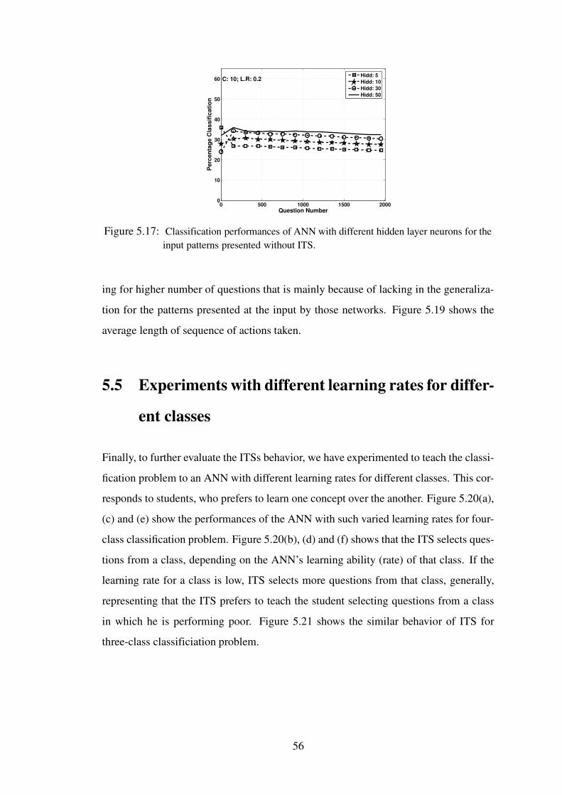
0 500 1000 1500 20000

10

20

30

40

50

60

Question NumberPe

rcen

tage

Cla

ssifi

catio

n

C: 10; L.R: 0.2 Hidd: 5Hidd: 10Hidd: 30Hidd: 50

Figure 5.17: Classification performances of ANN with different hidden layer neurons for theinput patterns presented without ITS.

ing for higher number of questions that is mainly because of lacking in the generaliza-

tion for the patterns presented at the input by those networks. Figure 5.19 shows the

average length of sequence of actions taken.

5.5 Experiments with different learning rates for differ-

ent classes

Finally, to further evaluate the ITSs behavior, we have experimented to teach the classi-

fication problem to an ANN with different learning rates for different classes. This cor-

responds to students, who prefers to learn one concept over the another. Figure 5.20(a),

(c) and (e) show the performances of the ANN with such varied learning rates for four-

class classification problem. Figure 5.20(b), (d) and (f) shows that the ITS selects ques-

tions from a class, depending on the ANN’s learning ability (rate) of that class. If the

learning rate for a class is low, ITS selects more questions from that class, generally,

representing that the ITS prefers to teach the student selecting questions from a class

in which he is performing poor. Figure 5.21 shows the similar behavior of ITS for

three-class classificiation problem.

56

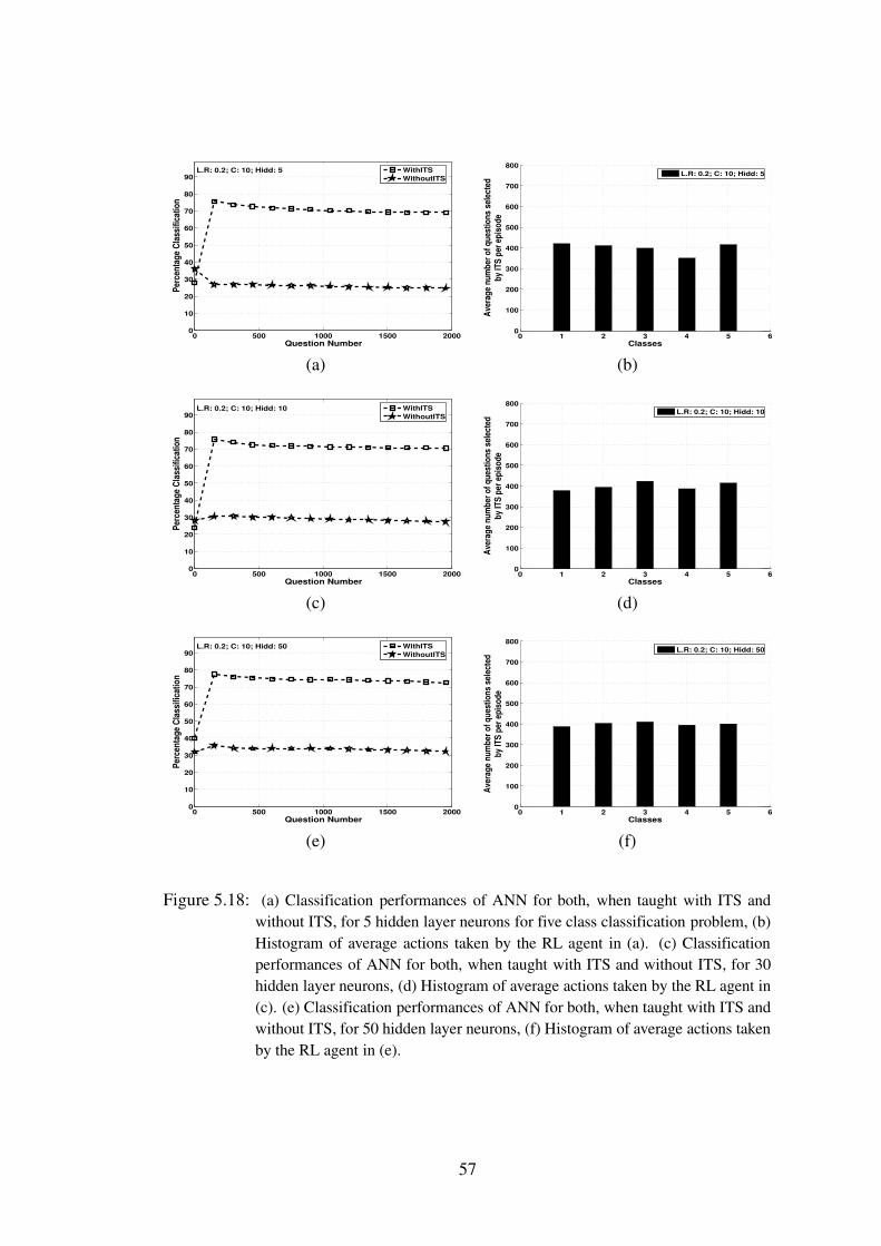
0 500 1000 1500 20000

10

20

30

40

50

60

70

80

90

Question Number

Perc

entag

e Clas

sifica

tion

L.R: 0.2; C: 10; Hidd: 5 WithITSWithoutITS

0 1 2 3 4 5 60

100

200

300

400

500

600

700

800

Classes

Aver

age n

umbe

r of q

uest

ions

selec

ted

by IT

S pe

r epi

sode

L.R: 0.2; C: 10; Hidd: 5

(a) (b)

0 500 1000 1500 20000

10

20

30

40

50

60

70

80

90

Question Number

Perc

entag

e Clas

sifica

tion

L.R: 0.2; C: 10; Hidd: 10 WithITSWithoutITS

0 1 2 3 4 5 60

100

200

300

400

500

600

700

800

Classes

Aver

age n

umbe

r of q

uest

ions

selec

ted

by IT

S pe

r epi

sode

L.R: 0.2; C: 10; Hidd: 10

(c) (d)

0 500 1000 1500 20000

10

20

30

40

50

60

70

80

90

Question Number

Perc

entag

e Clas

sifica

tion

L.R: 0.2; C: 10; Hidd: 50 WithITSWithoutITS

0 1 2 3 4 5 60

100

200

300

400

500

600

700

800

Classes

Aver

age n

umbe

r of q

uest

ions

selec

ted

by IT

S pe

r epi

sode

L.R: 0.2; C: 10; Hidd: 50

(e) (f)

Figure 5.18: (a) Classification performances of ANN for both, when taught with ITS andwithout ITS, for 5 hidden layer neurons for five class classification problem, (b)Histogram of average actions taken by the RL agent in (a). (c) Classificationperformances of ANN for both, when taught with ITS and without ITS, for 30hidden layer neurons, (d) Histogram of average actions taken by the RL agent in(c). (e) Classification performances of ANN for both, when taught with ITS andwithout ITS, for 50 hidden layer neurons, (f) Histogram of average actions takenby the RL agent in (e).

57

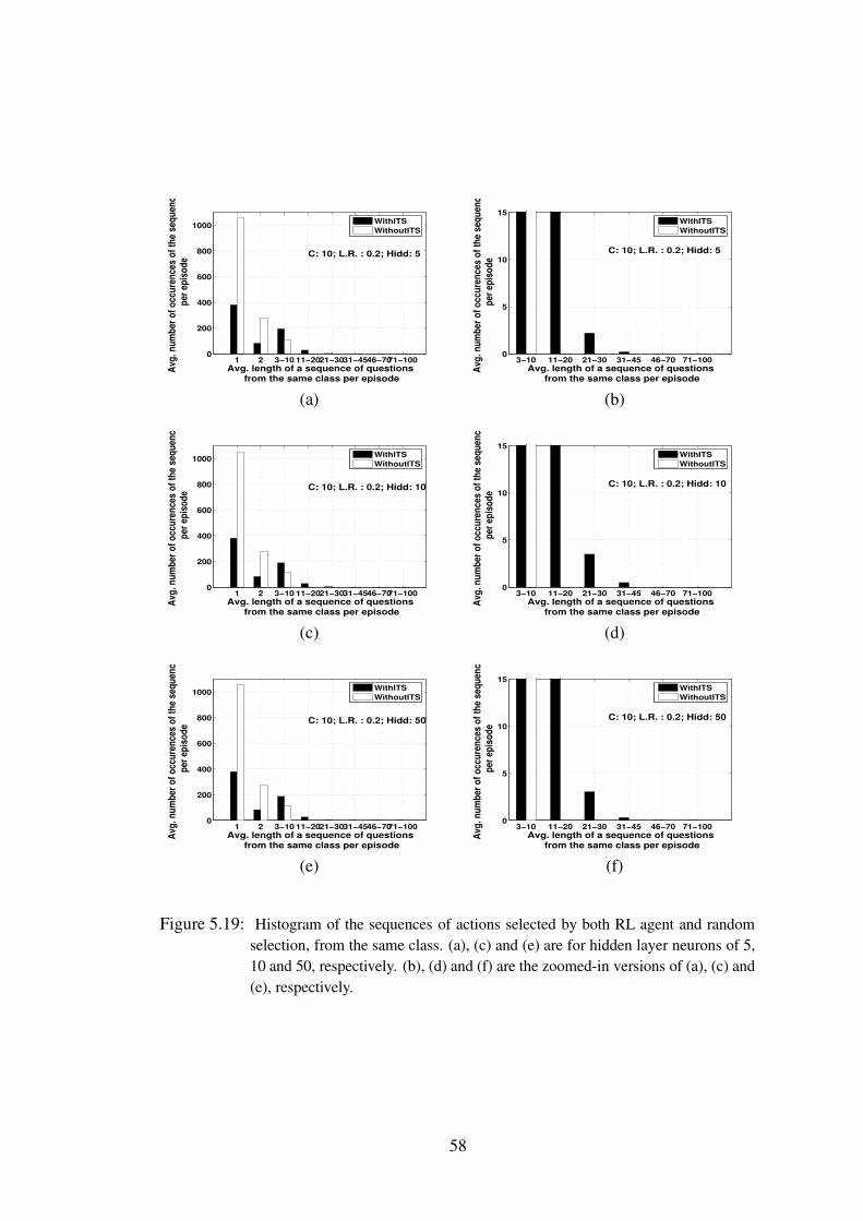
1 2 3−10 11−2021−3031−4546−7071−1000

200

400

600

800

1000

Avg. length of a sequence of questions from the same class per episode

Avg.

num

ber o

f occ

uren

ces o

f the

sequ

ence

per

episo

de

C: 10; L.R. : 0.2; Hidd: 5

WithITSWithoutITS

3−10 11−20 21−30 31−45 46−70 71−1000

5

10

15

Avg. length of a sequence of questions from the same class per episode

Avg.

num

ber o

f occ

uren

ces o

f the

sequ

ence

per

episo

de

C: 10; L.R. : 0.2; Hidd: 5

WithITSWithoutITS

(a) (b)

1 2 3−10 11−2021−3031−4546−7071−1000

200

400

600

800

1000

Avg. length of a sequence of questions from the same class per episode

Avg.

num

ber o

f occ

uren

ces o

f the

sequ

ence

per

episo

de

C: 10; L.R. : 0.2; Hidd: 10

WithITSWithoutITS

3−10 11−20 21−30 31−45 46−70 71−1000

5

10

15

Avg. length of a sequence of questions from the same class per episode

Avg.

num

ber o

f occ

uren

ces o

f the

sequ

ence

per

episo

deC: 10; L.R. : 0.2; Hidd: 10

WithITSWithoutITS

(c) (d)

1 2 3−10 11−2021−3031−4546−7071−1000

200

400

600

800

1000

Avg. length of a sequence of questions from the same class per episode

Avg.

num

ber o

f occ

uren

ces o

f the

sequ

ence

per

episo

de

C: 10; L.R. : 0.2; Hidd: 50

WithITSWithoutITS

3−10 11−20 21−30 31−45 46−70 71−1000

5

10

15

Avg. length of a sequence of questions from the same class per episode

Avg.

num

ber o

f occ

uren

ces o

f the

sequ

ence

per

episo

de

C: 10; L.R. : 0.2; Hidd: 50

WithITSWithoutITS

(e) (f)

Figure 5.19: Histogram of the sequences of actions selected by both RL agent and randomselection, from the same class. (a), (c) and (e) are for hidden layer neurons of 5,10 and 50, respectively. (b), (d) and (f) are the zoomed-in versions of (a), (c) and(e), respectively.

58

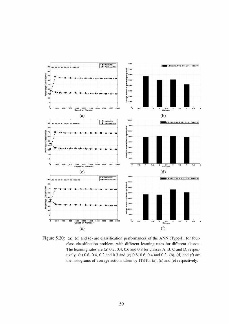
0 200 400 600 800 1000 1200 1400 1600 1800 20000

10

20

30

40

50

60

70

80

90

Question Number

Perc

entag

e Clas

sifica

tion

L.R: 0.2 0.4 0.6 0.8; C: 1; Hidd: 10WithITSWithoutITS

0 0.5 1 1.5 2 2.5 3 3.5 4 4.5 50

100

200

300

400

500

600

700

800

Classes

Aver

age n

umbe

r of q

uesti

ons p

er ep

isode

L.R.:0.2 0.4 0.6 0.8; C: 1; Hidd: 10

(a) (b)

0 200 400 600 800 1000 1200 1400 1600 1800 20000

10

20

30

40

50

60

70

80

90

Question Number

Perc

entag

e Clas

sifica

tion

L.R: 0.6 0.4 0.2 0.8; C: 10; Hidd: 10WithITSWithoutITS

0 0.5 1 1.5 2 2.5 3 3.5 4 4.5 50

100

200

300

400

500

600

700

800

Classes

Aver

age n

umbe

r of q

uesti

ons p

er ep

isode

L.R.:0.6 0.4 0.2 0.8; C: 10; Hidd: 10

(c) (d)

0 200 400 600 800 1000 1200 1400 1600 1800 20000

10

20

30

40

50

60

70

80

90

Question Number

Perc

entag

e Clas

sifica

tion

L.R: 0.8 0.6 0.4 0.2; C: 10; Hidd: 10WithITSWithoutITS

0 0.5 1 1.5 2 2.5 3 3.5 4 4.5 50

100

200

300

400

500

600

700

800

Classes

Aver

age n

umbe

r of q

uesti

ons p

er ep

isode

L.R.:0.8 0.6 0.4 0.2; C: 10; Hidd: 10

(e) (f)

Figure 5.20: (a), (c) and (e) are classification performances of the ANN (Type-I), for four-class classification problem, with different learning rates for different classes.The learning rates are (a) 0.2, 0.4, 0.6 and 0.8 for classes A, B, C and D, respec-tively. (c) 0.6, 0.4, 0.2 and 0.3 and (e) 0.8, 0.6, 0.4 and 0.2. (b), (d) and (f) arethe histograms of average actions taken by ITS for (a), (c) and (e) respectively.

59

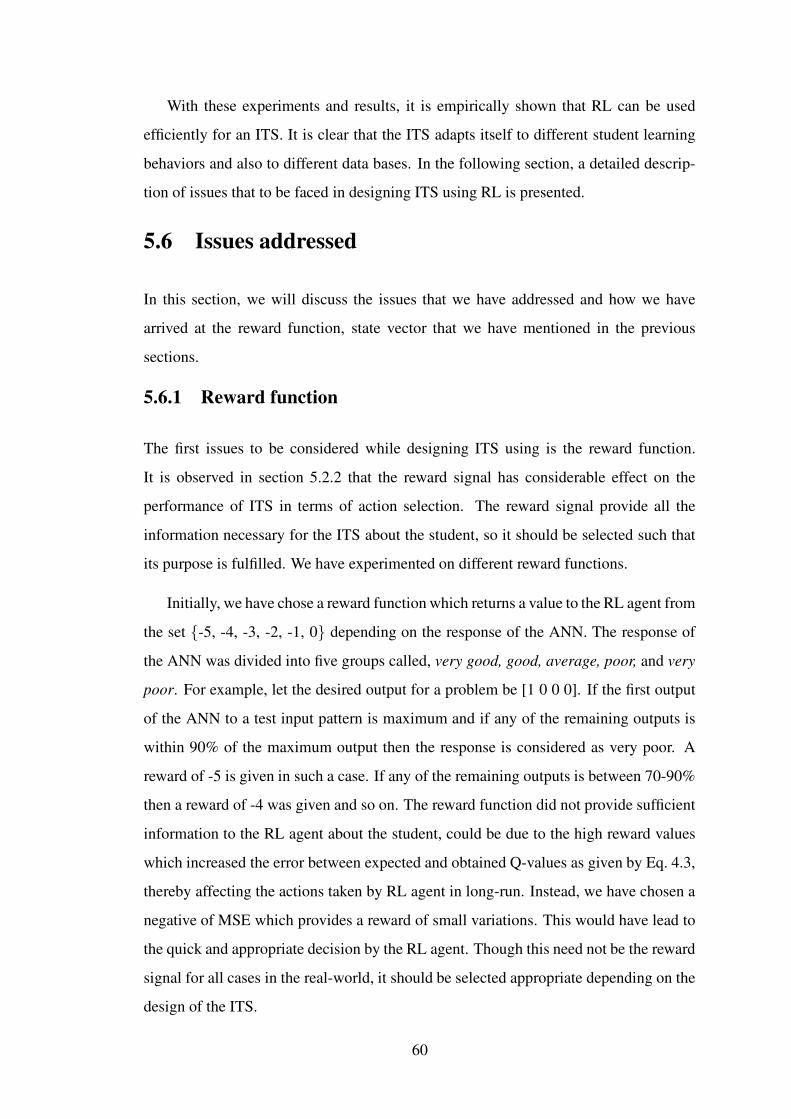
With these experiments and results, it is empirically shown that RL can be used

efficiently for an ITS. It is clear that the ITS adapts itself to different student learning

behaviors and also to different data bases. In the following section, a detailed descrip-

tion of issues that to be faced in designing ITS using RL is presented.

5.6 Issues addressed

In this section, we will discuss the issues that we have addressed and how we have

arrived at the reward function, state vector that we have mentioned in the previous

sections.

5.6.1 Reward function

The first issues to be considered while designing ITS using is the reward function.

It is observed in section 5.2.2 that the reward signal has considerable effect on the

performance of ITS in terms of action selection. The reward signal provide all the

information necessary for the ITS about the student, so it should be selected such that

its purpose is fulfilled. We have experimented on different reward functions.

Initially, we have chose a reward function which returns a value to the RL agent from

the set -5, -4, -3, -2, -1, 0 depending on the response of the ANN. The response of

the ANN was divided into five groups called, very good, good, average, poor, and very

poor. For example, let the desired output for a problem be [1 0 0 0]. If the first output

of the ANN to a test input pattern is maximum and if any of the remaining outputs is

within 90% of the maximum output then the response is considered as very poor. A

reward of -5 is given in such a case. If any of the remaining outputs is between 70-90%

then a reward of -4 was given and so on. The reward function did not provide sufficient

information to the RL agent about the student, could be due to the high reward values

which increased the error between expected and obtained Q-values as given by Eq. 4.3,

thereby affecting the actions taken by RL agent in long-run. Instead, we have chosen a

negative of MSE which provides a reward of small variations. This would have lead to

the quick and appropriate decision by the RL agent. Though this need not be the reward

signal for all cases in the real-world, it should be selected appropriate depending on the

design of the ITS.

60

0 500 1000 1500 20000

10

20

30

40

50

60

70

80

90

100

Question Number

Perc

entag

e Clas

sifica

tion

L.R: 0.2 0.4 0.6; C: 1; Hidd: 10

WithITSWithoutITS

0 0.5 1 1.5 2 2.5 3 3.5 40

100

200

300

400

500

600

700

800

900

1000

Classes

Aver

age n

umbe

r of q

uesti

ons p

er ep

isode L.R: 0.2 0.4 0.6; C: 1; Hidd: 10

(a) (b)

0 500 1000 1500 20000

10

20

30

40

50

60

70

80

90

100

Question Number

Perc

entag

e Clas

sifica

tion

L.R: 0.6 0.4 0.2; C: 1; Hidd: 10

WithITSWithoutITS

0 0.5 1 1.5 2 2.5 3 3.5 40

100

200

300

400

500

600

700

800

900

1000

Classes

Aver

age n

umbe

r of q

uesti

ons p

er ep

isode L.R: 0.6 0.4 0.2; C: 1; Hidd: 10

(c) (d)

0 500 1000 1500 20000

10

20

30

40

50

60

70

80

90

100

Question Number

Perc

entag

e Clas

sifica

tion

L.R: 0.6 0.8 0.2; C: 1; Hidd: 10

WithITSWithoutITS

0 0.5 1 1.5 2 2.5 3 3.5 40

100

200

300

400

500

600

700

800

900

1000

Classes

Aver

age n

umbe

r of q

uesti

ons p

er ep

isode L.R: 0.6 0.8 0.2; C: 1; Hidd: 10

(e) (f)

Figure 5.21: (a), (c) and (e) are classification performances of the ANN (Type-I), for three-class classification problem, with different learning rates for different classes.The learning rates are (a) 0.2, 0.4, and 0.6 for classes A, B, and C, respectively.(b) 0.6, 0.4, and 0.2 and (c) 0.6, 0.8 and 0.2. (b), (d) and (f) are the histogramsof average actions taken by ITS for (a), (c) and (e) respectively.

61

5.6.2 State representation

The state representation is the other major factor designer of an ITS using RL should

consider. As said earlier, the state variables model the behavior of the environment

(here student). As most of the RL algorithms apply to process where the state vari-

ables are selected in such a way that the state should satisfy the Markov property. For

example, initially we selected a state vector containing summary of past few ques-

tions asked i.e, the number of questions asked from each class and the number of very

good, good, average, poor and very poor responses to the questions from those classes

by the student, as state variables. The state vector for the four class problem was,

[NA NV GA NGA NAA NPA NVPA NB NV GB NGB NAB NPB NV PB NC NVGC NGC NAC NPC

NV PC ND NVGD NGD NAD NPD NVPD], where NA,NB,NC and ND are the number of

questions asked from classes A, B, C and D, respectively, and NVGB,NGB,NAB,NPB, and

NVPB are the number of very good, good, average, poor and very poor responses to the

questions from class B. This state vector was non-Markov as it was not providing much

clear information about the past states of the student. So, we have included a history of

past questions to make the state “more” Markov which suits RL framework both theo-

retically and practically. Though the RL framework may work better for non-Markov

states too, it is suggestible from the experiments that the state should be “near” to the

Markov states.

5.6.3 Domain module

The other issue that we have addressed is the domain module, and in turn the action

space. Initially, we divided the data space into different actions like, very easy ques-

tions, easy questions, average questions, hard questions and very hard questions, within

each class. The performance of ITS in such case was poor because of too many actions.

There were three different domain modules we experimented in section 5.1 each having

different classes and different action sets. The action set could even become finer by

considering different actions within a class. For example, generally for an ANN the

patterns around the boundary between two classes would be difficult to classify. So, we

can consider those patterns at boundary of each class as an action, which could increase

the performance of the ITS, but the action space should not be too large as explained in

62

section 4.4.2.

After this detailed description of the ITS and the validation of the ITS on the simu-

lated student, next chapter addresses the mapping of this ITS into the real-world situa-

tions, and the issues to be considered thereby in designing.

63

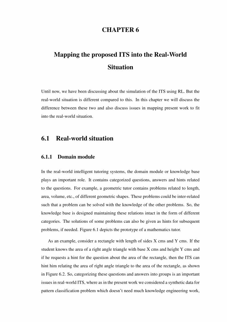
CHAPTER 6

Mapping the proposed ITS into the Real-World

Situation

Until now, we have been discussing about the simulation of the ITS using RL. But the

real-world situation is different compared to this. In this chapter we will discuss the

difference between these two and also discuss issues in mapping present work to fit

into the real-world situation.

6.1 Real-world situation

6.1.1 Domain module

In the real-world intelligent tutoring systems, the domain module or knowledge base

plays an important role. It contains categorized questions, answers and hints related

to the questions. For example, a geometric tutor contains problems related to length,

area, volume, etc., of different geometric shapes. These problems could be inter-related

such that a problem can be solved with the knowledge of the other problems. So, the

knowledge base is designed maintaining these relations intact in the form of different

categories. The solutions of some problems can also be given as hints for subsequent

problems, if needed. Figure 6.1 depicts the prototype of a mathematics tutor.

As an example, consider a rectangle with length of sides X cms and Y cms. If the

student knows the area of a right angle triangle with base X cms and height Y cms and

if he requests a hint for the question about the area of the rectangle, then the ITS can

hint him relating the area of right angle triangle to the area of the rectangle, as shown

in Figure 6.2. So, categorizing these questions and answers into groups is an important

issues in real-world ITS, where as in the present work we considered a synthetic data for

pattern classification problem which doesn’t need much knowledge engineering work,

Figure 6.1: Prototype of a Mathematics tutor

but could be an efficient problem for evaluating the ITS using simulated model of the

student.

6.1.2 Student model

The student model or state of the student we have considered gives information to the

ITS about the students’ performance by considering the number of questions asked and

the number of questions they have answered. But, for a human student, the student

model will be more complicated compared to this. While designing ITS, we could con-

sider the students’ time taken to respond, number of hints requested, his or her ability to

recollect concepts etc.,. The time taken by the student represents his or her confidence

and knowledge on the topic being taught. If the number of hints requested increases

indicating either students’ lack of knowledge or student is forgetting the concepts, then

ITSs should select questions varying in difficulty from low to high, such that the stu-

dents’ performance increases by improving his confidence, which has been proved that

by using ITSs the confidence level of a student can be improved [18]. The ability of the

student to recollect concepts can be evaluated by presenting same questions again in his

process of learning.

65

Figure 6.2: Prototype of a Mathematics tutor providing hint toa question on area of a rectangle

6.1.3 User-system interface

User-system interface is the medium through which the student and ITSs get feedback

about each other. Designing interface is another important issue to be considered while

developing an ITS. The interface should be designed such that the users feel comfortable

using it. The interface should also be designed to capture the attention of the student and

to increase his/her interest to use it. For example, Wayang outpost [20] uses cartoons

and graphics to grab the attention of the children and to ease them learning new concepts

by using it.

Figures 6.1 and 6.2 depicts a typical UI of a Mathematics Intelligent Tutoring Sys-

tem. Answers to a question are provided in multiple choices along with an option for

requesting hints.The user interface can be more attractive by using animations to attract

the attention of the students using it.

66

6.2 Mapping

After a brief presentation of the real-world scenario of ITS in the previous section, we

will look in this section how to map the present work of simulation into the real-world

problem.

6.2.1 Domain module

Let us consider the four class problem that was dealt in section 5.2, with the knowledge

base of synthetic patterns as shown in Figure 5.2. The patterns were divided into four

classes with each class consisting a set of patterns. The RL agent selects a pattern

from those classes and presents to the ANN for classification. These classes can be

considered as different categories of questions and hints that mentioned in section 6.1.1

while each pattern will maps to a question or hint in the real-world problem. These

categories of questions and hints form an action set for the RL agent. The RL agent

learns a policy to select a question from different categories in the domain module

developed for a particular subject, similar to as it selects a pattern from the synthetic

data set.

6.2.2 Student model or state representation

For an accurate estimation of the performance of a human student, the designer of an

ITS need to consider the factors discussed in section 6.1.2. For an ITS using RL, these

factors can be included in the state vector to represent the student’s knowledge. For

example, the student’s response time, T , can be included in the state vector as given by

[T NA NAC NAW NB NBC NBW NC NCC NCW ND NDC NDW xi−50 zi−50 xi−49 zi−49... xi−1

zi−1]. Similarly, other variable like number of hints requested also can be included in

the form of state variables. The state vector should be selected such that it doesn’t

violate Markov property greatly. One should also consider the other issues discussed in

section 4.4.2, while selecting the state vector.

We have discussed about the proposed ITS using reinforcement learning with its

real-world applications. This thesis will conclude with chapter 7 while discussing the

future work to be done depending on this work.

67

CHAPTER 7

Conclusion and Future work

In this thesis, we have designed an ITS which can adapt itself to different learning abil-

ities of students through interaction with them. It learns to teach according to the needs

of the student. For this purpose we have proposed an RL algorithm in chapter 4, for

taking pedagogical actions in an ITS. We have also presented, in the same chapter, the

teaching process with the proposes ITS. In chapter 5, the proposed ITS was experimen-

tally verified to teach students with different learning abilities. It has also been shown

that the RL agent adapts itself to the changes in the teaching environment, thus improv-

ing the performance of the student. It has been empirically proved that the reward signal

plays an important role in deciding the pedagogical actions by an RL agent. By consid-

ering the history and summary of past few questions asked, the state of the student can

be represented which would model the students learning behavior precisely.

We have also addressed the issues that arise while designing using RL as peda-

gogical module in the ITS. Though we have proved the adaptability of the ITS using

RL, there is still a lot of scope for improving this ITS as a solution to the present

pre-customized ITSs. In this work, we used state variables as a function of the past

questions, and negative of MSE of ANN output as reward signals. This ITS can also

be extended to real world problems like teaching mathematics, where selection of state

variables and action variables is more complex. In the real world situations, we can con-

sider the variables like the amount of time taken by the student to answer a question,

history of hints the student requested. More work can be done in selecting state vari-

ables, which can improve, not only the percentage classification but also the learning

rate. In this case, we have to consider which type of questions form a group, for exam-

ple, easy questions form a group and tough questions form another group. Selecting a

question from these groups could be the action set for the RL agent.

7.1 Summary of the contribution:• Proposed a reinforcement learning algorithm for ITS.

• Addressed issues related to state variables, reward function, and action set.

• Evaluated the adaptability of the proposed ITS using simulated students.

The proposed ITS could be further improved by using the hierarchical framework [38].

In a hierarchical framework, entire domain module is divided into lessons and each les-

son is divided into different categories. The RL agent has to learn two policies, one

for picking a lesson and the other for picking a categories within the lesson, which is

expected to improve the performance of the ITS.

7.2 Other Applications

Other applications of our work include pattern synthesis and active learning. Pattern

synthesis is the process of generating patterns for training and testing a machine. In our

case, the two dimensional data generated as a question can be considered as the pattern

synthesis problem. Active learning, is the ”learning with examples” [39]. This is a

closed-loop phenomenon of a learner asking questions that can influence the data added

to its training examples. In the case of ITS, the student has the facility to ask for hints for

improving his knowledge on the topic, this can be considered as active learning. Active

learning provides greatest reward in situations where data are expensive or difficult to

obtain.

69

REFERENCES

[1] B. S. Bloom, “The 2-Sigma Problem : The search for methods of group instructionas effective as one-to-one tutoring,” Educational Researcher, vol. 13(2), pp. 4–16,1984.

[2] J. Gordan, “ABC of learning and teaching in medicine,” British Medical Journal,vol. 326, pp. 553–545, March 2003.

[3] J. W. Regian, “Functional area analysis of intelligent computer-assisted instruc-tion,” TAPSTEM ICAI-FAA Committee, Brooks Air Force Base, Texas, 1997.

[4] J. Beck, M. Stern, and E. Haugsjaa, “Applications of AI in Education,” in ACMCrossroads, pp. 11–15, 1996.

[5] R. S. Sutton and A. G. Barto, Reinforcement Learning : An Introduction. Cam-bridge, MA: MIT Press, 1998.

[6] K. VanLehn, S. Ohlsson, and R. Nason, “Applications of simulated students: Anexploration,” Journal of Artificial Intelligence in Education, vol. 5(2), pp. 135–175, 1996.

[7] D. Sleeman and J. S. Brown, Intelligent Tutoring Systems. London: AcademicPress Inc., 1982.

[8] J. Beck and B. P. Woolf, “High-level student modeling with machine learning,”in Proceedings of Sixth International Conference on Intelligent Tutoring Systems,pp. 584–593, 2000.

[9] J. E. Beck and B. P. Woolf, “Using a learning agent with a student model,” inProceedings of Fourth International Conference on Intelligent Tutoring Systems,pp. 6–15, 1998.

[10] E. Aimeur, G. Brassard, H. Dufort, and S. Gambs, “CLARISSE : A machinelearning tool to initialize student models,” in Sixth International Conference onIntelligent Tutoring Systems, 2002.

[11] A. S. Gertner, C. Conati, and K. Lehn, “Procedural help in andes: Generating hintsusing a bayesian network student model,” in Proceedings of the Fifteenth NationalConference on Artificial Intelligence, pp. 106–111, 1998.

[12] M. Ikeda, K. Ashely, and T. W. Chan, eds., Improving Intelligent Tutoring Sys-tems: Using Expectation Maximization to Learn Student Skill Levels, vol. 4053 ofLecture Notes in Computer Science, (Berlin Heidelberg), Springer-Verlag, 2006.

[13] A. Jonsson, J. Johns, H. Mehranian, I. Arroyo, B. Woolf, A. Barto, D. Fisher, andS. Mahadevan, “Evaluating the feasibility of learning student models from data.”American Association for Artificial Intelligence(AAAI), 2005.

70

[14] R. Nkambou, B. Lefebvre, and G. Gauthier, “A curriculum-based student modelfor intelligent tutoring system,” in Fifth International Conference on User Mod-elling, pp. 91–98.

[15] P. Funk and O. Conlan, “Case-based reasoning to improve adaptability of intelli-gent tutoring systems,” in Workshop on Case-Based Reasoning for Education andTraining, CBRET’2002, (Aberdeen, Scotland), pp. 15–23, Robert Gordon Univer-sity, September 2002.

[16] R. H. Stottler and S. Ramachandran, “A case-based reasoning approach to inter-net intelligent tutoring systems (its) and its authoring,” in FLAIRS Conference,pp. 181–186, 1999.

[17] P. Funk and O. Conlan, “Using case-based reasoning to support authors of adaptivehypermedia systems.”

[18] C. R. Beal, “Gaining confidence in Mathematics : Instructional technology forgirls,” in International Conference on Mathematics/Science Education & Tech-nology (M/SET 2000), (San Diego, CA), March 2000.

[19] J. E. Beck, B. P. Woolf, and C. R. Beal, “ADVISOR: A machine learning ar-chitecture for intelligent tutor construction,” in Proceedings of the 17th NationalConference On Artificial Intelligence, 2000.

[20] C. R. Beal, I. Arroyo, J. M. Royer, and B. P. Woolf, “Wayang Outpost: An intel-ligent multimedia tutor for high stakes math achievement tests.” Accepted to theAmerican Educational Research Association annual meeting, April 2003.

[21] K. N. Martin and I. Arroyo, “AgentX: Using Reinforcement Learning to Improvethe Effectiveness of Intelligent Tutoring Systems.,” in Intelligent Tutoring Sys-tems, pp. 564–572, 2004.

[22] K. D. Forbus and P. J. Feltovich, Smart machines in education. Cambridge,MA:MIT Press/AAAI Press, 2001.

[23] C. R. Eliot and B. P. Woolf, “Reasoning about the user within a simulation-basedreal-time training system,” in Fourth International Conference on User Modeling,(Hyannis, Cape Cod, Mass., U.S.A), August 1994.

[24] C. R. Eliot and B. P. Woolf, “An adaptive student-centered curriculum for an In-telligent Tutoring System,” vol. 5(1), pp. 67–86, 1995.

[25] E. A. Domeshek, E. Holman, and S. Luperfoy, “Discussion control in an auto-mated Socratic tutor,” in Interservice/Industry Training, Simulation, and Educa-tion Conference (I/ITSEC), 2004.

[26] ComMentor, “Intelligent tutoring for command thinking skills.” Army ResearchInstitute Newsletter, May 2003.

[27] M. R. Kretchmar and C. W. Anderson, “Comparison of CMACs and radial basisfunctions for local function approximators in reinforcement learning,” in Proceed-ings of the International Conference on Neural Networks, ICNN’97, (Houston,Texas, USA), 1997.

71

[28] B. Yegnanarayana, Artificial Neural Networks. New Delhi, India: Printice-Hall ofIndia Private Limited, 2004.

[29] J. S. Albus, “A theory of cerebellar function,” Mathematical Biosciences, vol. 10,pp. 25–61, 1971.

[30] J. Moody and C. Darken, “Learning with localized receptive fields,” in Proceed-ings of the 1988 Connectionist Models Summer School, (Morgan Kaufmann Pub-lishers, San Mateo, CA), pp. 133–143, 1989.

[31] C. J. C. H. Watkins, Learning from Delayed Rewards. PhD thesis, CambridgeUniversity, 1989.

[32] G. A. Rummery and M. Niranjam, “On-line Q-learning using connectionist sys-tems,” CUED/F-INFENG/TR 166, Engineering Department, Cambridge Univer-sity, 1994.

[33] C. W. Anderson, “Q-learning with hidden-unit restarting,” in Proceedings of FifthInternational Conference on Neural Information Processing Systems, pp. 81–88,1992.

[34] R. E. Bellman, Dynamic Programming. Princeton: Princeton University Press,1957.

[35] I. L. Cohen, “An artificial neural network analogue of learning in autism,” Biolog-ical Psychiatry, vol. 36, no. 1, pp. 5–20, 1994.

[36] I. L. Cohen, “A neural network model of autism : Implications for theory andtreatment,” in Neuroconstructivism : Perspectives and Prospects (D. Mareschal,S. Sirois, G. Westermann, and M. H. Johnson, eds.), vol. 2, Oxford UniversityPress, Oxford, UK, 2006.

[37] NICHD, “Autism and Genes.” A Report published by National Institute of ChildHealth and Human Development (NIH Publication No. 05-5590), U. S. Depart-ment of Health and Human Services, May 2005.

[38] A. Barto and S. Mahadevan, “Recent advances in hierarchical reinforcement learn-ing,” Discrete Event Dynamic Systems: Theory and Applications, vol. 13, pp. 343–379, 2003.

[39] D. A. Cohn, Z. Ghahramani, and M. I. Jordan, “Active learning with statisticalmodels,” Journal of Artificial Intelligence Research, vol. 4, pp. 129–145, 1996.

72

LIST OF PAPERS BASED ON THESIS

1. Sreenivasa Sarma B. H., and Ravindran B., Intelligent Tutoring Systems usingReinforcement learning to teach Autistic students. Accepted for publicationin the International Conference on Home/ Community Oriented ICT for the NextBillion (HOIT’07), Chennai, August-2007.

73